Convergence in Human Decision-Making Dynamics∗†

Ming Cao Andrew Stewart Naomi Ehrich LeonardMechanical and Aerospace Engineering

Princeton University, Princeton, NJ 08544{mingcao, arstewar, naomi}@princeton.edu

Abstract

A class of binary decision-making tasks called the two-alternative forced-choice task has beenused extensively in psychology and behavioral economics experiments to investigate human deci-sion making. The human subject makes a choice between two options at regular time intervalsand receives a reward after each choice; for a variety of reward structures, these experiments showconvergence of the aggregate behavior to rewards that are often suboptimal. In this paper wepresent two models of human decision making: one is the Win-Stay, Lose-Switch (WSLS) modeland the other is a deterministic limit of the popular Drift Diffusion (DD) model. With thesemodels we prove convergence of the human behavior to the observed aggregate decision makingfor reward structures with matching points. The analysis is motivated by human-in-the-loopsystems, where humans are often required to make repeated choices among finite alternatives inresponse to evolving system performance measures. We discuss application of the convergenceresult to design of human-in-the-loop systems using a map from the human subject to a humansupervisor.

Keywords: human decision making; two-alternative forced-choice task; win-stay, lose-switch model;drift diffusion model; robotic foraging; explore vs. exploit

1 Introduction

The superior ability of humans to handle the unexpected and to recognize pattern and extractstructure from data makes human decision making invaluable to performance of complex tasks inuncertain, changing environments. However, without computational aid, human decision makers maybe overwhelmed by the many elements and the multitude of scales in complex, time-varying systems.This suggests an important role for automation, where fast, dedicated data processing and feedbackresponsiveness can be exploited. Indeed, there has been much research in cooperative control ofmulti-agent robotic systems for automating cooperative tasks, see e.g., the collections [1, 2, 3, 4].And yet, fully automated decision making presents serious limitations to performance: automatingoptimal decisions in complex tasks in uncertain, time-varying settings will typically require solvingintractable, nonlinear, stochastic, optimization problems. Even when good suboptimal decisionsare designed into robotic decision makers, there will likely remain unanticipated, and thus poorlyaddressed, scenarios. Further, attempts to increase the versatility of the completely automatedsystem can lead to unverifiable code.

The problem of integrating the efforts of humans and robots in demanding tasks has driven therapidly growing fields of human-robot interaction and social robotics. For example, in [5] Simmons et∗This research was supported in part by AFOSR grant FA9550-07-1-0-0528 and ONR grant N00014–04–1–0534.†Accepted for publication in Systems and Control Letters, December 2009

1

al have developed a framework and tools to coordinate robotic assembly teams with remote humanoperators for performing construction and assembly in hazardous environments. Their approachallows for adjustable autonomy where control of tasks can change between the human and the roboticteam. To conserve on human expertise, the robot team operates autonomously and only requestshelp from the human supervisor as needed. Using a similar notion of sliding autonomy, Kauppand Makarenko [6] examine a human-robot communication system for information exchange in anavigation task. In [7] Steinfeld et al define common metrics to evaluate human-robot interactionperformance. Alami et al [8] propose a robot control architecture that explicitly considers andmanages its interaction with a human. The authors point out the critical challenge in representingthe humans. Trafton and co-authors directly address this challenge by studying human-humaninteraction and then embedding the human behavior into the robots. For example, Trafton et al[9] study videotape of astronauts-in-training performing cooperative assembly tasks and use theempirical data to inform cognitive models of perspective-taking. They embed these models intorobots to improve their ability to work collaboratively with humans.

These works make clear that profitable integration of human and robot decision-making dynamicsshould take advantage of strengths of human decision makers as well as strengths of robotic agents.They also make clear that a major challenge in achieving this goal is understanding how humansmake decisions and what are their associated strengths and weaknesses. Since psychologists andbehavioral scientists explore these very questions, a central tenet of our approach is to leverage theexperimental and modeling work of psychologists and behavioral scientists on human decision making.To do this we seek commonality in the kinds of decisions humans make in complex tasks and thekinds of decisions humans make in psychology experiments. We focus here on a well-studied class ofsequential binary decision making called the two-alternative forced-choice task [10, 11, 12, 13, 14, 15].In this task, the human subject in the psychology experiments chooses between two options atregular time intervals and receives a reward after each choice that depends on recent past decisions.Interestingly, these experiments show convergence of the aggregate behavior to rewards that areoften suboptimal. This suboptimal behavior is of particular interest for what it can tell us aboutdynamics of human-in-the-loop systems. Indeed, just like in the two-alternative forced-choice task, ahuman in the loop performing a supervisory task is often required to choose repeatedly between finitealternatives in response to an update on system performance that in turn depends on current andpast decisions. Examples include human supervisory control of multiple unmanned aerial vehicleswhere the supervisor must decide between attending to targets and ensuring safe return of vehicles[16] and human operator control of air traffic where the operator must decide between grounding orscheduling vehicles [17].

In this paper, we seek to formally describe the convergence behavior observed in experiment;the goal is to better understand conditions of suboptimal human decision making and to providea framework for designing improved human-in-the-loop systems. We present two models of humandecision making in the two-alternative forced-choice task: the Win-Stay Lose-Switch (WSLS) modeland the Drift Diffusion (DD) model. With these models we prove convergence to matching behaviorfor reward structures with matching points. Intuitively, this implies that the decision maker convergesto a neighborhood in decision space of a decision sequence which results in a reward that stays roughlyconstant with each subsequent choice. These convergence results are consistent with experimentalobservations [10, 18]. A partial version of our convergence results in the case of WSLS appears in[19]. We note that Montague and Berns [11] showed that the matching point is an attracting point inthe DD model in the case that a couple of simplifying assumptions hold. In [20] Vu and Morgansenperform an analysis of the WSLS model in a related context using finite state machines.

As one possible application of the convergence results, we introduce a human-supervised collectiverobotic foraging problem, where a group of robots in the field moves around and collects a distributed

2

resource and a human supervisor repeatedly makes a decision to assign the role of each of therobots, either to be an explorer or an exploiter of resource. The human and robots work as a teamto maximize resource collected: the robots follow efficient, collaborative exploring and exploitingstrategies and the human tries to make the best allocation decisions.

We review studies of the two-alternative forced-choice task in Section 2. In Section 3, we presentthe WSLS and DD decision-making models. We prove convergence to matching for each of thesemodels in Section 4. In Section 5 we present, and investigate with a simulation study, a map fromthe decision-making task of a human supervisor of a robotic foraging team to the two-alternativeforced-choice task. We make final remarks in Section 6.

2 Two-Alternative Force-Choice Tasks

Real-world decision-making problems are difficult to study since the reward for a decision usuallydepends in a nontrivial way on the decision history. Many studies have considered decision-rewardrelationships that are fixed; however, these have limited value in addressing problems associated withcomplex, time-varying tasks like the ones motivating this paper. Here, we briefly review a class ofdecision-making tasks called the two-alternative forced-choice task, where reward depends on pastdecisions.

Montague et al. [14, 11] introduced a dynamic economic game with a series of decision-rewardrelationships that depend on a subject’s decision history. The human subject is faced with a two-alternative sequential choice task. Choices of either A or B are made sequentially (forced withinregular time intervals) and a reward for each decision is administered directly following the choice.Without knowing the reward structure, the human subject tries to maximize the total reward (sumof individual rewards).

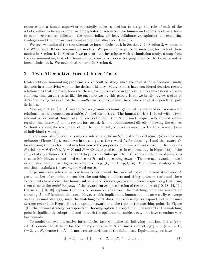
Two reward structures frequently considered are the matching shoulders (Figure 1(a)) and risingoptimum (Figure 1(b)). As shown in these figures, the reward fA for choosing A and the reward fBfor choosing B are determined as a function of the proportion y of times A was chosen in the previousN trials (y = #A’s/N). N = 20 and N = 40 are typical choices in experiments. In Figure 1(a), if thesubject always chooses A, the reward drops to 0.2. Subsequently, if B is chosen, the reward jumps upclose to 0.9. However, continued choices of B lead to declining reward. The average reward, plottedas a dashed line on each figure, is computed as yfA(y) + (1 − y)fB(y). The optimal strategy is theone that maximizes the average reward curve.

Experimental studies show how humans perform at this task with specific reward structures. Agreat number of experiments consider the matching shoulders and rising optimum tasks and theseexperiments have shown that human subjects tend, on average, to adopt choice sequences y that bringthem close to the matching point of the reward curves (intersection of reward curves) [10, 18, 14, 11].Herrnstein [10, 18] explains that this is reasonable since near the matching point the reward forchoosing A or B is about the same. However, this implies that humans do not necessarily convergeon the optimal strategy, since the matching point does not necessarily correspond to the optimalaverage reward. In Figure 1(a), the optimal reward is to the right of the matching point. In Figure1(b), the optimal strategy corresponds to choosing option A every time. The reward at the matchingpoint is significantly suboptimal and to reach the optimum the subject may first have to endure verylow rewards.

To model the two-alternative forced-choice task we define the following notation. Let x1(t) ∈{A,B} denote the decision for the binary choice A or B at time t and let xi(t) = x1(t − i + 1),i = 2, . . . , N , denote the N − 1 most recent decisions of the finite past. Equivalently, we have

xi(t+ 1) = xi−1(t), i = 2, . . . , N, t = 0, 1, 2, . . . . (1)

3

(a) Matching shoulders. (b) Rising optimum.

Figure 1: Reward curves. The dotted line depicts fA, the reward for choice A. The solid line depictsfB, the reward for choice B. The dashed line is the average value of the reward. Each is plottedagainst the proportion of choice A made in the last N decisions.

Let y denote the proportion of choice A in the last N decisions, i.e.,

y(t) =1N

N∑i=1

δiA(t) (2)

where

δiA(t) ={

1 if xi(t) = A0 if xi(t) = B.

Note that y can only take value from a finite set Y of N + 1 discrete values:

Y = {j/N, j = 0, 1, . . . , N}.

The reward at time t is given by

r(t) ={fA(y(t)) if x1(t) = AfB(y(t)) if x1(t) = B .

(3)

Thus, the two-alternative forced-choice task can be modeled as an N -dimensional, discrete-timedynamical system, described completely by equations (1)-(3) where xi(t), 1 ≤ i ≤ N , is the state ofthe system and y(t) is the output of the system.

3 Decision-Making Models

The matching tendency in humans and animals was first identified by Herrnstein [10, 18], whoserelated work has been influential in quantitative analysis of behavior and mathematical psychol-ogy. However, few mathematically provable results on matching behavior have been obtained andreported. This is, in part, due to the difficulty in modeling the dynamics of human and animaldecision making. Several models have been proposed to describe the dynamics of human decisionmaking, and in this paper we analyze two of them. One is the Win-Stay, Lose-Switch (WSLS) model,also known as Win-Stay, Lose-Shift, which has been used in psychology, game theory, statistics and

4

machine learning [21, 22]. The other is a deterministic limit of a popular stochastic reinforcementlearning model, called the Drift Diffusion (DD) model, which was introduced by Egelman et al. [14]and further studied in [11] and [12]. It should be noted that many of the other models which havebeen proposed are, in fact, equivalent to the DD model [23].

3.1 WSLS Model

The subject’s decision dynamics may be affected by all the decisions and rewards in the last N trials.In fact, a goal of the studies of two-alternative forced-choice tasks is to determine the decision-making mechanism through experiment and use behavioral and neurobiological arguments to justifythe likelihood of the mechanism. The WSLS model assumes that decisions are made with informationfrom the rewards of the previous two choices only and that a switch in choice is made when a decreasein reward is experienced. That is, the subject repeats the choice from time t at time t + 1 if thereward at time t is greater than or equal to that at time t− 1; otherwise, the opposite choice is usedat time t+ 1:

x1(t+ 1) ={x1(t) if r(t) ≥ r(t− 1);x1(t) otherwise,

t = 1, 2, 3, . . . (4)

where · denotes the “not” operator; i.e., if x1(t) = A (x1(t) = B), then x1(t) = B (x1(t) = A).

3.2 A Deterministic Limit of the DD Model

In the context of multi-choice decision-making dynamics, a one-dimensional drift diffusion processcan be described by a stochastic differential equation [24, 15, 25]:

dz = αdt+ σdW, z(0) = 0 (5)

where z represents the accumulated evidence in favor of a candidate choice of interest, α is the driftrate representing the signal intensity of the stimulus acting on z and σdW is a Wiener process withstandard deviation σ which is the diffusion rate representing the effect of white noise. Now considerthe two-alternative forced-choice task with choices A and B. The drift rate α, as described in [14, 12],is determined by a subject’s anticipated rewards for a decision of A or B, denoted ωA and ωB.

Take z to be the accumulated evidence for choice A less the accumulated evidence for choice B.Then on each trial a choice is made when z(t) first crosses the predetermined thresholds ±ν. Inwhich case, if ν is crossed choice A is made and if −ν is crossed choice B is made. For such driftdiffusion processes, as pointed out in [15], it can be computed using tools developed in [23] that theprobability of choosing A is

pA(t) =1

1 + e−µ(ωA(t)−ωB(t))(6)

where µ is determined by the threshold-to-drift ratio να , and ωA − ωB is determined by the signal-

to-noise ratio ασ .

To gain insight into the mechanics of the DD model, we choose a specific set of relevant param-eters. Specifically, we study the deterministic limit of the decision rule (6) deduced from the DDmodel by letting µ in (6) go to infinity. Then at time t > 0, the subject chooses A if ωA(t) > ωB(t)and B if ωA(t) < ωB(t). In the event that ωA = ωB, we assume that humans are of an explorativenature, and thus the subject uses the opposite of the last choice. To summarize,

x1(t) =

A if ωA(t) > ωB(t)B if ωA(t) < ωB(t)x1(t− 1) if ωA(t) = ωB(t)

t = 1, 2, 3, . . . (7)

5

where as in (4), · denotes the “not” operator.We are now left with modelling the transition of the anticipated rewards ωA and ωB. Using data

collected in neurobiological studies of the role of dopamine neurons in coding for reward predictionerror [26], and guided by temporal difference learning theory [27], the following difference equationshave been proposed to describe the update of ωA and ωB. Let Z(t) ∈ {A,B} be the choice made attime t, then

ωZ(t)(t+ 1) = (1− λ)ωZ(t)(t) + λr(t) (8)ωZ(t)(t+ 1) = ωZ(t)(t) t = 0, 1, 2, . . . (9)

where r(t) is the reward at time t. Here, λ ∈ [0, 1] is called the learning rate, which reflects how theanticipated reward of choice Z(t) at t+ 1 is affected by its value at t.

In the update model (8) and (9), referred to as the standard model in the sequel, when a choiceof Z is made the value of ωZ remains unchanged because without memory no reward information forZ is available. A more sophisticated update model, called the eligibility trace model, is constructedin [12]. It takes into account the effect of memory by updating both ωA and ωB continually. Theeligibility trace can be interpreted as a description of how psychological perception of informationrefreshes or decays in response to whether or not an external stimulus is enforced. The eligibilitytraces (as presented in [12]) denoted by φA(t) and φB(t) for choices A and B respectively, evolveaccording to

φZ(t)(t+ 1) = 1 + φZ(t)(t)e− 1τ (10)

φZ(t)(t+ 1) = φZ(t)(t)e− 1τ (11)

with initial values φA(0) = φB(0), where τ > 0 is a parameter that determines the decaying effectsof memories.

With the eligibility traces included, ωA and ωB are updated according to

ωA(t+ 1) = ωA(t) + λ[r(t)− ωZ(t)(t)]φA(t) (12)ωB(t+ 1) = ωB(t) + λ[r(t)− ωZ(t)(t)]φB(t) (13)

where the eligibility traces φA and φB act as time-varying weighting factors. When τ is chosen tobe small, the update rule in the eligibility trace model (12) and (13) reduces to that in the standardmodel (8) and (9).

To analyze the impact of the dynamics of the eligibility traces on the evolution of ωA and ωB,we discretize the eligibility traces φA and φB. We set the learning rate λ in (12) and (13) to beits maximum value (λ = 1) which corresponds to the current reward having the strongest possibleinfluence on the subject. Then

ωA(t+ 1) = ωA(t) + [r(t)− ωZ(t)(t)]φA(t) (14)ωB(t+ 1) = ωB(t) + [r(t)− ωZ(t)(t)]φB(t). (15)

We discretize φA and φB as follows. For σ ∈ {A,B}, if σ is the last choice made, we set the value ofφσ to be saturated at one because the impact of the current reward has been accounted for by settingλ to be its maximum value. We let φσ decay to zero once the opposite choice σ has been chosenconsecutively. This corresponds to the situation when, without external stimulus, the memory fadesquickly. When a switch in choice is made (from σ at time t− 1 to σ at time t), let the fresh memory

6

of the unchosen alternative, φσ, be a small, positive number ε ∈ (0, 1). Then φA and φB take valuesin {0, ε, 1} and evolve according to

φσ(t) =

1 if σ = x1(t)ε if σ = x1(t) = x1(t− 1)0 if σ = x1(t) = x1(t− 1)

t = 1, 2, 3, . . . (16)

The resulting model is a deterministic limit of the DD with eligibility traces.

4 Convergence Analysis

In this section, we give a rigorous analysis of the dynamics of human performance in games withmatching shoulders rewards. It is shown that for both of the human decision-making models, theproportion y of choice A converges to a neighborhood of the matching point. It should be noted thatconvergence also applies for reward structures that contain the matching shoulders structure locally(as in the rising optimum example of Figure 1(b)).

Denote by y∗ the value of y at the matching point, i.e., the intersection of the two curves fA andfB. We consider the generic case when

y∗ /∈ Y, (17)

i.e., y∗ is not an integer multiple of 1/N . In the non-generic case, when y∗ ∈ Y, a tighter convergenceresult applies. Let yl denote the greatest element in Y that is smaller than y∗ and let yu denote thesmallest element in Y that is greater than y∗. Let yl

′= yl − 1/N and yu

′= yu + 1/N . Define

L ∆= [yl, yu] and L′ ∆= [yl′, yu

′].

So that L′ is well defined, let 1/N < y∗ < (N − 1)/N and N ≥ 3.

4.1 Convergence of the WSLS Model

In this section, we analyze the convergence behavior of the system (1)-(4). We consider reward curvessuch that fA decreases monotonically and fB increases monotonically with increasing y, i.e.,

d

dyfA(y) < 0,

d

dyfB(y) > 0, ∀y ∈ [0, 1] . (18)

This includes the linear matching shoulders curves of Figure 1(a) as well as a more general class ofnonlinear reward curves. It also includes the rising optimum reward curves of Figure 1(b) locallyabout the matching point. We prove both a local and a global convergence result to the matchingpoint. The local result is applicable to reward structures that have a local matching point and satisfy(18) for y in a neighborhood of y∗. This includes the rising optimum reward curves of Figure 1(b). Toformally preclude limit cycles about points other than the matching point it is necessary to requirethat

13≤ y∗ ≤ 2

3. (19)

The convergence results apply for general N ≥ 6. For lower values of N the system degeneratesand the output y may converge to 0 or 1. The linear curves used in the experiments [11] satisfy theconditions (17), (18) and (19), so the analysis in this section provides an analytical understandingof human decision-making dynamics in two-alternative forced-choice tasks of the same type.

7

4.1.1 Local convergence

The following result describes the oscillating behavior of y(t) near y∗.

Theorem 1 For system (1)-(4) satisfying conditions (17)-(19), if y(t1) ∈ L for some t1 > 0, theny(t) ∈ L′ for all t ≥ t1.

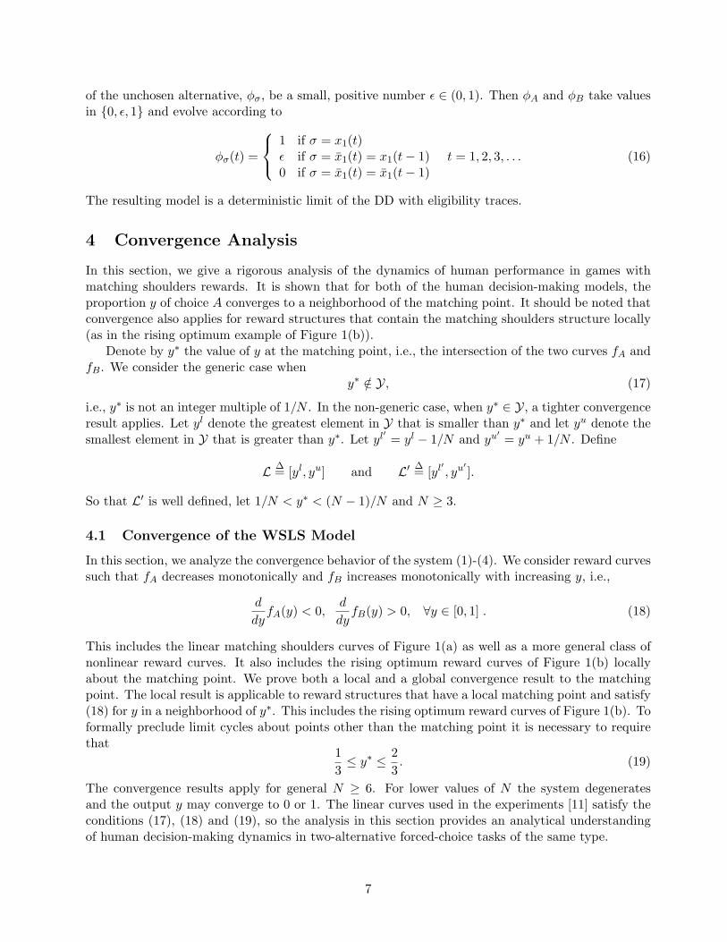
Before we prove Theorem 1, let us first examine a typical trajectory starting at time t = t1 withy(t1) ∈ L. Consider the matching shoulders reward structure shown in Figure 2 as an example. Webring attention to four points on the reward curves. As shown in Figure 2 (which represents onepossible configuration of these four points for general matching shoulders reward curves), we denotep1 = (yl, fA(yl)), p2 = (yl, fB(yl)), p3 = (yu, fA(yu)) and p4 = (yu, fB(yu)).

Figure 2: Points p1, p2, p3, and p4 used to examine trajectories around the matching point.

Suppose we are given a set of initial conditions y(t1) = yu, x1(t1) = A, x20(t1) = B and supposex1(t1 + 1) = B. Then y(t1 + 1) = y(t1) = yu and the reward r(t1 + 1) = fB(yu) > fA(yu) = r(t1). Inview of (4), we know that x1(t1 + 2) = B. If xN (t1 + 1) = A, then y(t1 + 2) = y(t1 + 1)− 1/N = yl

and r(t1 + 2) = fB(yl) < fB(yu) = r(t1 + 1). Again by (4), it must be true that x1(t1 + 3) = A.Suppose xN (t+ 2) = B, then y(t1 + 3) = yu.

To track the above system trajectory in Figure 2 for t1 ≤ t ≤ t1 + 3, one can find that thetrajectory moves from p3, to p4, to p2 and back to p3. Hence, one may conjecture that once y(t)enters L, it will stay in L. However, this is not the case. Consider a counterexample, namely inFigure 2 the system trajectory again starts at p3. However, let xN (t1) = B and x1(t1 +1) = A. Theny(t1 + 2) = yu + 1/N /∈ L. Although L is not an invariant set for y(t), trajectories of y(t) startingin L will always remain in L′. This is an intuitive interpretation of Theorem 1.

To prove Theorem 1, we first prove the following four lemmas.

Lemma 1 For system (1)-(4), with conditions (17)-(19) satisfied, if x1(t1) = A, x1(t1 + 1) = A andy(t1) < 1 for some t1 ≥ 0, then there exists 0 ≤ τ ≤ N such that y(t) = y(t1) for t1 ≤ t ≤ t1 + τ andy(t1 + τ + 1) = y(t1) + 1/N .

Proof of Lemma 1: If xN (t1) = B, then y(t1 + 1) = y(t1) + 1/N . So the conclusion holds forτ = 0. On the other hand, if xN (t1) = A, then y(t1 + 1) = y(t1) and r(t1 + 1) = fA(y(t1 + 1)) =fA(y(t1)) = r(t1). According to (4), x1(t1 + 2) = A. In fact the choice of A will be repeatedly chosen

8

as long as the value of xN remains A. However, since y(t1) < 1, there must exist 0 ≤ τ < N suchthat xN (t) = A for t1 ≤ t ≤ t1 + τ and xN (t1 + τ + 1) = B. Accordingly, the conclusion holds. �

One can prove the following lemma, the counterpart to Lemma 1, with a similar argument.

Lemma 2 For system (1)-(4), with conditions (17)-(19) satisfied, if x1(t1) = B, x1(t1 +1) = B andy(t1) > 0 for some t1 ≥ 0, then there exists 0 ≤ τ ≤ N such that y(t) = y(t1) for t1 ≤ t ≤ t1 + τ andy(t1 + τ + 1) = y(t1)− 1/N .

Now we further study behavior of the system when its trajectory is on the left of the matchingpoint y∗.

Lemma 3 For system (1)-(4), with conditions (17)-(19) satisfied, if y(t1) < y∗ and y(t1 + 1) =y(t1)− 1/N > 0 for some t1 ≥ 0, then there exists 0 ≤ τ ≤ N such that

y(t) = y(t1)− 1/N for t1 ≤ t ≤ t1 + τ (20)

andy(t1 + τ + 1) = y(t1). (21)

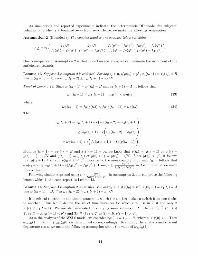
Proof of Lemma 3: We find it convenient to prove this lemma by labeling the following fourpoints: s1 = (y(t1), fA(y(t1))), s2 = (y(t1), fB(y(t1))), s3 = (y(t1) − 1/N, fA(y(t1) − 1/N)), s4 =(y(t1)− 1/N, fB(y(t1)− 1/N)), as shown in Figure 3.

We denote the reward values at these four points by r|si , i = 1, . . . , 4. Then r(t1) = r|s1 or

Figure 3: Points s1, s2, s3, s4, s5, and s6 used in the proofs of Lemma 3 and Lemma 7.

r|s2 . Since y(t1 + 1) < y(t1), it must be true that x1(t1 + 1) = B, then r(t1 + 1) = r|s4 . Sincer|s4 < r|s2 < r|s1 , we know x1(t1 + 2) = A. So at t1 + 2, the system trajectory moves from s4 toeither s1 or s3. If the former is true, the conclusion holds for τ = 2. If the latter is true, sincer|s3 > r|s4 , it follows that x1(t1 + 3) = A. By applying Lemma 1, we know (20) and (21) hold. �

Similarly, we consider the situation when y(t1) > y∗ and y(t1 + 1) = y(t1) + 1/N < 1 forsome t1 ≥ 0. Denote four points: r1 = (y(t1), fA(y(t1))), r2 = (y(t1), fB(y(t1))), r3 = (y(t1) +1/N, fA(y(t1) + 1/N)) and r4 = (y(t1) + 1/N, fB(y(t1) + 1/N)). Using the fact that r|r3 < r|r1 < r|r2and a similar argument as that in the proof of Lemma 3, we can prove the following result.

9

Lemma 4 For system (1)-(4), with conditions (17)-(19) satisfied, if y(t1) > y∗ and y(t1 + 1) =y(t1) + 1/N for some t1 ≥ 0, then there exists 0 ≤ τ ≤ N such that

y(t) = y(t1) + 1/N for t1 ≤ t ≤ t1 + τ (22)

andy(t1 + τ + 1) = y(t1). (23)

Now we are in a position to prove Theorem 1.Proof of Theorem 1: If y(t) ∈ L for all t ≥ t1, then the conclusion holds trivially. Now suppose

this is not true. Let t2 > t1 be the first time for which y(t) /∈ L. Then it suffices to prove the claimthat the trajectory of y(t) starting at y(t2) stays at y(t2) for a finite time and then enters L. Notethat y(t2) equals either yl − 1/N or yu + 1/N . Suppose y(t2) = yl − 1/N , then the claim followsdirectly from Lemma 3; if on the other hand, y(t2) = yu + 1/N , then the claim follows directly fromLemma 4. �

4.1.2 Global convergence

Theorem 1 gives the convergence analysis in the neighborhood L of the matching point y∗. Our nextstep is to present the global convergence analysis for the system (1)-(4). It is easy to check that if thesystem starts with the initial condition y(0) = 0 and x1(1) = B or the initial condition y(0) = 1 andx1(1) = A, then the trajectory of y(t) will stay at its initial location. It will also be shown that wheny∗ < 1

3 or y∗ > 23 , a limit cycle of period three not containing y∗ may appear. Thus it is necessary

that condition (19) is satisfied, i.e., 13 ≤ y∗ ≤ 2

3 . In what follows we show that if the trajectory ofy(t) starts in (0, 1) and conditions (17), (18) and (19) are satisfied, then the trajectory always entersL after a finite time.

Proposition 1 For any initial condition of the system (1)-(4) satisfying 0 < y(0) < 1 with condi-tions (17)-(19) satisfied, there is a finite time T > 0 such that y(T ) ∈ L.

To prove Proposition 1, we need to prove the following four lemmas.

Lemma 5 For system (1)-(4), with conditions (17)-(19) satisfied, if y(t1) < y∗, y(t1 + 1) = y(t1)and x1(t1 + 1) 6= x1(t1) for some t1 ≥ 0, then there exists a finite τ > 0 such that

y(t1 + τ) = y(t1) + 1/N. (24)

Proof of Lemma 5: There are two cases to consider. (a) Suppose x1(t1 +1) = A and x1(t1) = B.Since y(t1 + 1) = y(t1) < y∗, we know r(t1 + 1) = fA(y(t1 + 1)) = fA(y(t1)) > fB(y(t1)) = r(t1), sox1(t1 + 2) = A. Then the conclusion follows from Lemma 1. (b) Now suppose instead x1(t1 + 1) = Band x1(t1) = A. Again since y(t1 + 1) = y(t1) < y∗, we know r(t1 + 1) = fB(y(t1 + 1)) = fB(y(t1)) <fA(y(t1)) = r(t1), so x1(t1+2) = A. As a result, either y(t1+2) = y(t1)+1/N or y(t1+2) = y(t1+1).If the former is true, then the conclusion holds for τ = 2; if the latter is true, then the discussionreduces to that in (a). �

Using a similar argument, one can prove the following lemma, which is the counterpart to Lemma5.

Lemma 6 For system (1)-(4), with conditions (17)-(19) satisfied, if y(t1) > y∗, y(t1 + 1) = y(t1)and x1(t1 + 1) 6= x1(t1) for some t1 ≥ 0, then there exists a finite τ > 0 such that

y(t1 + τ) = y(t1)− 1/N. (25)

10

Now we show that the system will approach the matching point.

Lemma 7 For system (1)-(4), with conditions (17)-(19) satisfied, if 0 < y(t1) < yl and y(t1 + 1) =y(t1)− 1/N for some t1 ≥ 0, then there exists a finite τ > 0 such that

y(t1 + τ) = y(t1) + 1/N. (26)

Proof of Lemma 7: Denote the six points s1 = (y(t1), fA(y(t1))), s2 = (y(t1), fB(y(t1))), s3 =(y(t1)−1/N, fA(y(t1)−1/N)), s4 = (y(t1)−1/N, fB(y(t1)−1/N)), s5 = (y(t1)+1/N, fA(y(t1)+1/N))and s6 = (y(t1) + 1/N, fB(y(t1) + 1/N)), as shown in Figure 3. Since y(t1 + 1) < y(t1), it must betrue that x1(t1 + 1) = B. If x1(t1) = A, we know from t1 to t1 + 1, the system trajectory moves froms1 to s4. Since r(t1 + 1) = r|s4 < r|s1 = r(t1), we know x1(t1 + 2) = A. Then at t1 + 2, the trajectorymoves to either s1 or s3. We discuss these two cases separately.(a) If at t1 + 2 the trajectory moves to s1. Since r|s1 > r|s4 , it follows that x1(t1 + 3) = A. In viewof Lemma 1, the conclusion holds.(b) If at t1 + 2, the trajectory moves to s3, since r|s3 > r|s4 , we know x1(t1 + 3) = A. FromLemma 1, there exists a finite time t2 < N at which the trajectory moves from s3 to s1. Becauser|s1 < r|s3 , we have x1(t2 + 1) = B. Then at time t2 + 1, the trajectory moves to either s2 or s4.Now we discuss two sub-cases. (b1) Suppose the former is true, that the trajectory goes to s2. Theconclusion follows directly from Lemma 5. (b2) Suppose the latter is true, that the trajectory goesto s4. Because r|s4 < r|s1 , x1(t2 + 2) = A. Then y(t) will remain strictly less than y(t1) + 1/N ifa cycle of s4 → s3 → s1 → s4 is formed. In fact, from the analysis above, this is the only potentialscenario in case (b2) where y(t) < y(t1) + 1/N for all t ≥ t1. Were such a cycle to appear, A wouldbe chosen at least twice as often as B. However, because y(t1) < yl = y∗− 1/N < 1

3 , it must be truethat the proportion of A in xi(t1), 1 ≤ i ≤ N , is less than 1

3 . Thus such a cycle can never happen.So the conclusion also holds for the sub-case (b2).

If on the other hand, x1(t1) = B, we know from t1 to t1 + 1, the system trajectory movesfrom s2 to s4. Since r|s4 < r|s2 , we know x1(t1 + 2) = A. So at t1 + 2, the trajectory moves tos3 or s1. If the former is true, the discussion reduces to ruling out the possibility of forming acycle of s4 → s3 → s1 → s4 which we have done in (b2). Otherwise, if the latter is true, sincer|s1 > r|s4 , we know x1(t1 + 3) = A. From Lemma 1 we know there exists a finite time t3 at whichy(t3) = y(t1) + 1/N , and thus the conclusion holds for τ = t3 − t1.Combining the above discussions, we conclude that the proof of Lemma 7 is complete. �

Using Lemmas 2, 6 and a similar argument as in the proof of Lemma 7, one can prove thefollowing lemma which is the counterpart to Lemma 7.

Lemma 8 For system (1)-(4), with conditions (17)-(19) satisfied, if yu < y(t1) < 1 and y(t1 + 1) =y(t1) + 1/N for some t1 ≥ 0, then there exists a finite τ > 0 such that

y(t1 + τ) = y(t1)− 1/N. (27)

Now we are in a position to prove Proposition 1.Proof of Proposition 1: For any 0 < y(0) < 1, either y(1) = y(0) + 1/N , or y(1) = y(0), or

y(1) = y(0)− 1/N . We will discuss these three possibilities in each of two cases. First consider thecase where y(0) < yl. If y(1) = y(0)− 1/N , according to Lemma 7, there is a finite time t1 for whichy(t1) > y(0). If y(1) = y(0) and x1(1) 6= x1(0), according to Lemma 5, there is a finite time t2 forwhich y(t2) > y(0). If y(1) = y(0) and x(1) = x(0) = A, according to Lemma 1, there is a finitetime t3 for which y(t3) > y(0). If y(1) = y(0) and x(1) = x(0) = B, according to Lemma 2, there isa finite time t4 for which y(t4− 1) = y(0) and y(t4) = y(t4− 1)− 1/N . Then according to Lemma 7,

11

there is a finite time t4 for which y(t4) > y(0). So for all possibilities of y(1) there is always a finitetime t ∈ {1, t1, t2, t3, t4} for which y(t) > y(0). Using this argument repeatedly, we know that thereexists a finite time T1 at which y(T1) = yl ∈ L. Now consider the other case where y(0) > yu, thenusing similar arguments, one can check that there exists a finite time T2 for which y(T2) = yu ∈ L.Hence, we have proven the existence of T which lies in the set {T1, T2}. �

Combining the conclusions in Theorem 1 and Proposition 1, we have proven the following theorem,which describes the global convergence property of y(t).

Theorem 2 For any initial condition of the system (1)-(4) satisfying 0 < y(0) < 1 with conditions(17)-(19) satisfied, there exists a finite time T > 0 such that for any t ≥ T , y(t) ∈ L′.

4.2 Convergence of the DD Model

In this section we prove convergence of y(t) in the DD model with eligibility trace for matchingshoulders reward structures. All results in this subsection apply to the system (1)-(3), (7) and (14)-(16). As in the analysis for the WSLS model, we consider the general case (17) when y∗ /∈ Y. Alsolike the analysis for the WSLS model, the results generalize to nonlinear curves; however, for clarityof presentation we specialize to intersecting linear reward curves defined by

fA(y) = kAy + cA

fB(y) = kBy + cB (28)

where kA < 0, kB > 0 and cA, cB > 0.We first look at the case when the subject does not switch choice at a given time t0.

Lemma 9 For any t0 > 0, if y(t0 − 1) < 1 and x1(t0 − 1) = x1(t0) = A, then there exists a finitet1 ≥ t0 such that x1(t) = A for all t0 ≤ t ≤ t1 and y(t1) = y(t0 − 1) + 1/N .

Proof of Lemma 9: If xN (t0 − 1) = B, then y(t0) = y(t0 − 1) + 1/N and so the conclusion holdsfor t1 = t0. If on the other hand xN (t0 − 1) = A, then y(t0) = y(t0 − 1). From (16) we know thatφA(t0 − 1) = φA(t0) = 1 and φB(t0) = 0. Then it follows from (14) that ωA(t0 + 1) = r(t0) =fA(y(t0)) = fA(y(t0 − 1)) = ωA(t0) and from (15) that ωB(t0 + 1) = ωB(t0). Since x1(t0 − 1) =x1(t0) = A, from (7) it must be true that ωA(t0) > ωB(t0). Thus we know ωA(t0 + 1) > ωB(t0 + 1),so again from (7), we have x1(t0 + 1) = A. In fact, the choice of A will be repeatedly chosen aslong as the value of xN remains A. However, since y(t0 − 1) < 1, there must exist t1 ≤ t0 + Nsuch that xN (t1 − 1) = B and then for the same t1, we have x1(t) = A for all t0 ≤ t ≤ t1, andy(t1) = y(t0 − 1) + 1/N . �

Using a similar argument, one can prove the following lemma which is the counterpart to Lemma9.

Lemma 10 For any t0 ≥ 0, if y(t0 − 1) > 0 and x1(t0 − 1) = x1(t0) = B, then there exists a finitet1 ≥ t0 such that x1(t) = B for all t0 ≤ t ≤ t1, and y(t1) = y(t0 − 1)− 1/N .

Lemmas 9 and 10 imply that if Z ∈ {A,B} is repeatedly chosen, then the anticipated rewardfor choice Z decreases as a result of the change in y while the anticipated reward for the alternativeZ stays the same because the eligibility trace φZ remains zero. Hence, a switch of choices is likelyto happen after a finite time. Now we look at the case when the subject switches choice at timet0 > 0, namely x1(t0) = x1(t0 − 1). Then from (16), we have φx1(t0−1)(t0) = ε; correspondinglyfrom update rules (14) and (15), we have ωx1(t0−1)(t0 + 1) = ωx1(t0−1)(t0) + ε(r(t0)−ωx1(t0−1)(t0)) =ωx1(t0−1)(t0) + ε(ωx1(t0−1)(t0 + 1) − ωx1(t0−1)(t0)). Hence, the magnitude of ε is critical in updating

12

the value of the anticipated reward when a switch of choices happens. It should be pointed out thatin Section 3, to be consistent with the exponential decay rate for eligibility trace in [12], we havemade an assumption that ε is a small number. This assumption can be stated by restricting theupper bound for the convex combination of points on the fA and fB lines.

Assumption 1 (Restricted Convex Combination) For y ∈ Y,

(1− ε) min{fA(y), fB(y)}+ εmax{fA(y), fB(y)} < fA(y∗) = fB(y∗).

The following result states that under certain circumstances the subjects will not immediatelyfollow a switch of choice with another switch of choice.

Lemma 11 Suppose Assumption 1 is satisfied. For any t0 > 0, if x1(t0) = A, x1(t0 − 1) = B andy(t0−1) < y∗, then there exists a finite t1 ≥ t0 such that x1(t) = A for all t0 ≤ t ≤ t1, and y(t1) > y∗.

Proof of Lemma 11: From (16) we know that φA(t0) = 1 and φB(t0) = ε. So from (14) and (15), itfollows that

ωB(t0) = r(t0 − 1) = fB(y(t0 − 1)), (29)

ωA(t0 + 1) = r(t0) = fA(y(t0)), (30)

andωB(t0 + 1) = ωB(t0) + ε(r(t0)− ωA(t0)) = ωB(t0) + ε(fA(y(t0))− ωA(t0)). (31)

Since x1(t0) = A, from (7) it must be true that ωA(t0) ≥ ωB(t0). Combining with (31), we have

ωB(t0 + 1) ≤ ωB(t0) + ε(fA(y(t0))− ωB(t0)) = (1− ε)ωB(t0) + εfA(y(t0)).

Substituting (29), we have

ωB(t0 + 1) ≤ (1− ε)fB(y(t0 − 1)) + εfA(y(t0)).

Since x1(t0) = A and x1(t0 − 1) = B, we know y(t0) = y(t0 − 1) or y(t0) = y(t0 − 1) + 1/N . Sincey(t0 − 1) < y∗, it must be true that either y(t0) = yu or y(t0) ≤ yl. We consider these two casesseparately. Case (a): y(t0) = yu. Set t1 = t0, then y(t1) > y∗ holds trivially. Case (b): y(t0) ≤ yl.Then fA(y∗) < fA(y(t0)) ≤ fA(y(t0 − 1)). Also,

ωB(t0 + 1) ≤ (1− ε)fB(y(t0 − 1)) + εfA(y(t0 − 1)) < fA(y∗),

where the last inequality follows from Assumption 1. Combining these with (30) we know that

x1(t0 + 1) = A (32)

and consequently φA(t0 + 1) = 1 and φB(t0 + 1) = 0. In fact, A will be repeatedly chosen, φA andφB will remain one and zero respectively until some finite time t1 > t0 for which ωA(t1) = r(t1) =fA(y(t1)) is less than or equal to ωB(t0 + 1) or y(t1) = 1. Since ωB(t0 + 1) < fA(y∗), it follows thaty(t1) > y∗. So we have proved the conclusion for case (b) and the proof is complete. �

Using a similar argument, one can prove the following lemma which is the counterpart to Lemma11.

Lemma 12 Suppose Assumption 1 is satisfied. For any t0 > 0, if x1(t0) = B, x1(t0 − 1) = Aand y(t0 − 1) > y∗, then there exists a finite t1 ≥ t0 such that x1(t) = B for all t0 ≤ t ≤ t1, andy(t1) < y∗.

13

As simulations and reported experiments indicate, the deterministic DD model fits subjects’behavior only when ε is bounded away from zero. Hence, we make the following assumption:

Assumption 2 (Bounded ε) The positive number ε is bounded below satisfying

ε ≥ max{

−kA/NfA(yl′)− fB(yl′)

,kB/N

fB(yu′)− fA(yu′),fA(yu

′)− fB(yl

′)

fA(yl)− fB(yl),fB(yl

′)− fA(yu

′)

fB(yu)− fA(yu)

}.

One consequence of Assumption 2 is that in certain scenarios, we can estimate the increment of theanticipated rewards.

Lemma 13 Suppose Assumption 2 is satisfied. For any t0 > 0, if y(t0) < yl′, x1(t0−1) = x1(t0) = B

and x1(t0 + 1) = A, then ωB(t0 + 2) ≥ ωB(t0 + 1)− kA/N .

Proof of Lemma 13: Since x1(t0 − 1) = x1(t0) = B and x1(t0 + 1) = A, it follows that

ωB(t0 + 1) ≤ ωA(t0 + 1) = ωA(t0) < ωB(t0) (33)

whereωB(t0 + 1) = fB(y(t0)) < fB(y(t0 − 1)) = ωB(t0). (34)

Then

ωB(t0 + 2) = ωB(t0 + 1) + ε

(ωA(t0 + 2)− ωA(t0 + 1)

)≥ ωB(t0 + 1) + ε

(ωA(t0 + 2)− ωB(t0)

)= ωB(t0 + 1) + ε

(fA(y(t0 + 1))− fB(y(t0 − 1))

).

From x1(t0 − 1) = x1(t0) = B and x1(t0 + 1) = A, we know that y(t0) = y(t0 − 1) or y(t0) =y(t0 − 1) − 1/N and y(t0 + 1) = y(t0) or y(t0 + 1) = y(t0) + 1/N . Since y(t0) < yl

′, it follows

that y(t0 + 1) ≤ yl′

and y(t0 − 1) ≤ yl′. Because of the monotonicity of fA and fB, it follows that

ωB(t0 + 2) ≥ ωB(t0 + 1) + ε(fA(yl′) − fB(yl

′)). Using ε ≥ −kA/N

fA(yl′ )−fB(yl′ )in Assumption 2, we reach

the conclusion. �Following similar steps and using ε ≥ kB/N

fB(yu′ )−fA(yu′ )in Assumption 2, one can prove the following

lemma which is the counterpart to Lemma 13.

Lemma 14 Suppose Assumption 2 is satisfied. For any t0 > 0, if y(t0) > yu′, x1(t0−1) = x1(t0) = A

and x1(t0 + 1) = B, then ωA(t0 + 2) ≥ ωA(t0 + 1) + kB/N .

It is critical to examine the time instances at which the subject makes a switch from one choiceto another. Thus let T denote the set of time instances for which t > 0 is in T if and only ifx1(t) 6= x1(t − 1). We are also interested in studying some subsets of T . Define TA

∆= {t : t ∈T , x1(t) = A, y(t− 1) < y∗} and TB

∆= {t : t ∈ T , x1(t) = B, y(t− 1) > y∗}.As in the analysis of the WSLS model, we consider xi(0), i = 1, . . . , N , where 0 < y(0) < 1. Then

ωx1(0)(1) = r(0) = fx1(0)(y(0)) is determined correspondingly. To simplify the analysis and rule outdegenerate cases, we make the following assumption about the value of ωx1(0)(1).

14

Assumption 3 (Bounded ωx1(0)(1)) Let 0 < y(0) < 1 and ωx1(0)(1) = fx1(0)(y(0)). The initial valueωx1(0)(1) satisfies

ωx1(0)(1) < ωx1(0)(1), (35)

ωx1(0)(1) < fA(y∗), (36)

andωx1(0)(1) > max{fA(1), fB(0), fA(1) + (kB + kA)/N, fB(0)− (kB + kA)/N}. (37)

Now we are ready to study how the DD model with the eligibility trace evolves with time.

Lemma 15 Suppose all the Assumptions 1 - 3 are satisfied. Then,

T = TA ∪ TB.

Proof of Lemma 15: From (35) we know that x1(1) = x1(0) and in fact x1(0) will be repeatedlychosen until the reward for choosing x1(0) is below ωx1(0)(1). Such a switch will always happenbecause of (37). Let t0 denote the time at which such a switch happens, i.e., x1(t0 − 1) = x1(0)and x1(t0) = x1(0). In view of (36), we know that y(t0 − 1) < y∗ if x1(0) = B and y(t0 − 1) > y∗

if x1(0) = A. So t0 ∈ TA if x1(0) = B and t0 ∈ TB if x1(0) = A, and thus t0 ∈ TA ∪ TB. Byinspection, if y(t0 − 1) ∈ L, then either Lemma 9 or Lemma 10 is applicable to t0; if on the otherhand, y(t0 − 1) /∈ L, then either Lemma 11 or 12 is applicable to t0. This implies that x1(t0) willbe repeatedly chosen such that the time of the next switch t1 ≥ t0 satisfies t1 ∈ Tx1(t0) ⊂ TA ∪ TB.Further, Lemmas 9 - 12 can be applied again to t1. Then, by induction, we know all time instancesfor which a switch happens belong to TA ∪ TB. �

As becomes apparent later, when the DD model with the eligibility trace converges, the values ofy∗, kA and kB affect the range of the interval containing y∗ to which y(t) converges. In this paper,we are interested in the sufficient condition under which such an interval is L′.

Assumption 4 is concerned with the relative positions of points on the reward lines fA and fBcorresponding to values of y in L′.

Assumption 4 (Points in L′)

fB(yl) + ε(fA(yu)− fB(yu)) ≥ fA(yu′), (38)

fA(yu) + ε(fB(yl)− fA(yl)) ≥ fB(yl′). (39)

Proposition 2 Suppose all the Assumptions 1-4 are satisfied. If t0 ∈ T , y(t0 − 1) ∈ L′, theny(t) ∈ L′ for all t ≥ t0.

Proof of Proposition 2: The conclusion can be proved by induction if we can prove the followingfact: There is always a finite t1 > t0 such that t1 ∈ T and y(t) ∈ L′ for all t0 ≤ t ≤ t1. In order toprove this fact, we need to consider four cases.

• Case (a): x1(t0) = A and y(t0 − 1) = yl′. Then

ωB(t0 + 1) > fB(yl′) + ε

(fA(y(t0))− fB(yl)

)≥ fB(yl

′) + ε

(fA(yl)− fB(yl)

),

where the first inequality holds since fB(yl) > fB(yl′) and the last inequality holds because

fA(y(t0)) ≥ fA(yl). In view of the inequality ε ≥ fA(yu′)−fB(yl

′)

fA(yl)−fB(yl)in Assumption 2 and combining

with Lemma 11, we know that there is always a finite t1 > t0 such that t1 ∈ TB and y(t) ∈ L′for all t0 ≤ t ≤ t1.

15

• Case (b): x1(t0) = A and y(t0 − 1) = yl. Then

ωB(t0 + 1) ≥ fB(yl) + ε

(fA(y(t0))− ωA(t0)

)> fB(yl) + ε

(fA(yu)− fB(yu)

),

where the first inequality holds because ωA(t0) ≥ ωB(t0) and the last inequality holds becausefA(y(t0)) ≥ fA(yu) and ωA(t0) = ωA(t0 − 1) < ωB(t0 − 1) = fB(y∗) < fB(yu). Then in view of(38), we know ωB(t0 + 1) ≥ fA(yu

′), and so there is always a finite t1 > t0 such that t1 ∈ TB

and y(t) ∈ L′ for all t0 ≤ t ≤ t1.

• Case (c): x1(t0) = B and y(t0 − 1) = yu. Following similar steps as in case (b) and using (39),we know there is always a finite t1 > t0 such that t1 ∈ TA and y(t) ∈ L′ for all t0 ≤ t ≤ t1.

• Case (d): x1(t0) = B and y(t0 − 1) = yu′. Following similar steps as in (a) and using the

inequality ε ≥ fB(yl′)−fA(yu

′)

fB(yu)−fA(yu) in Assumption 2 and combining with Lemma 12, we know thatthere is always a finite t1 > t0 such that t1 ∈ TA and y(t) ∈ L′ for all t0 ≤ t ≤ t1.

In view of the discussion in cases (a)-(d), we conclude that the proof is complete. �

Proposition 3 Suppose all the Assumptions 1-4 are satisfied. There is always a finite T ∈ T forwhich y(T − 1) ∈ L′.

Proof of Proposition 3: From (37) in Assumption 3, we know that x1(0) cannot be repeatedly chosenfor more than N times, and thus there is t0 ∈ TA ∪ TB. If y(t0 − 1) ∈ L′, then set T = t0 and wereach the conclusion. If on the other hand, y(t0 − 1) /∈ L′, then either Lemma 13 or 14 applies tot0− 1. Without loss of generality, suppose Lemma 13 applies, then ωB(t0 + 1) ≥ ωB(t0)− kA/N . By(37) ωB(t0 + 1) > fA(1). So, there exists a t1 which is the smallest element in TB such that t1 > t0.Then ωA(t1) ≥ ωB(t0 + 1) + kA/N > ωB(t0). In fact, one can check that switches will continue toexist and ωx1(t) will be a monotonically strictly increasing function until ωx1(t) reaches either fA(yu

′)

or fB(yl′) at some finite time T ′. Set T to be the smallest element in T that is greater than T ′, then

it must be true that y(T − 1) ∈ L′. �Combining Propositions 2 and 3, we have proved the main result of this section.

Theorem 3 For system(1)-(3), (7), (14)-(17) and (28), if Assumptions 1-4 are satisfied, then thereexists a finite T > 0, such that y(t) ∈ L′ for all t ≥ T .

4.3 Discussion

We have proved in Theorems 2 and 3 for the WSLS decision-making model and the DD decision-making model that the proportion y of A’s in the moving window of the N most recent decisionsconverges to the neighborhood L′ of the matching point y∗. This means that eventually the decisionmaker confines decisions to those corresponding to the four values of y closest to y∗. However,convergence is more direct for the WSLS decision maker as compared to the DD decision maker. Inthe case of the WSLS decision maker, the very first time y reaches L, it will remain in L′ for allfuture time. This is because the WSLS makes its greedy decisions between A and B depending onlyon the two most recent awards. On the other hand, in the case of the DD decision maker, if thesame choice is made repeatedly when y is in L′ (and thus in L), then y can pass through L′ withoutgetting trapped. It is only when the decision maker switches choice while y ∈ L′ that y will remainin L′ for all future time. The DD decision maker can persist with repeated choices even as rewards

16

decrease because the expected reward for the alternative, which depends on the reward received thelast time the alternative was chosen, can be relatively low.

In the psychology studies, N is chosen large enough to push the limits of what humans canremember. N can be interpreted as a measure of task difficulty since it determines how many of thepast choices influence the present reward. N controls the resolution of the reward: reward dependson y, which takes value in the set Y = {j/N, j = 0, 1, . . . , N}. The convergence we have shown istighter for larger N , i.e., L and L′ are smaller. Likewise, the convergence rate is slower for larger Nsince it will take more choices to make the same magnitude change in y. The resolution also affectssensitivity of decision making: peaks and dips in the reward curve of width smaller than 1/N won’tbe measured by the decision maker. For example, in the rising optimum reward (Figure 1(b)), asmall enough N would enable the decision maker to “jump over” the minimum in the fA curve.

5 Application

As one possible application of the convergence results of Section 4, we formulate a human-supervisedrobotic foraging problem where the human makes sequential binary decisions. To make the theory ap-plicable, we propose a map from the human-supervised robotic foraging problem to a two-alternativeforced-choice task. We discuss conditions for such a map that would justify using results on humandecision making to help guide the design of an integrated human-robot system. We are particularlyinterested in leveraging the matching behavior phenomenon since it is so strongly supported by psy-chology experiments and is formally proven in the previous section. However, we expect that thehuman supervisor will contribute to the complex foraging task in a variety of ways for which theremay not be extensive insight nor formal models. Accordingly, we do not aim to use the existingmodels of human decision making to replace the human. The map proposed here is only a first stepand we expect that alternatives will improve and extend our central idea of identifying and leveragingparallels between what human subjects do in psychology experiments and what human operators doin complex tasks. Our focus is on human-in-the-loop issues; examples of developed strategies usefulfor collective foraging include exploration [28], coverage [29] and gradient climbing [30].

The robotic foraging problem that we are interested in is partly motivated by the producer-scrounger (PS) foraging game that models the behavior of group-foraging animals [31, 32]. Thismodel has been successful in predicting animals’ decisions either to look for food (produce) or toexploit the food found by other foragers (scrounge). Two results in the study of the PS game areespecially relevant to the robotic foraging problem of interest. First, the rewards for producingand scrounging are functions of the proportion of scroungers in the animal group, and such rewardcurves are similar to the matching shoulders curves studied in Section 4 [31]. Second, scientists in arecent field study have introduced techniques to manipulate the reward curves in order to predictablyshift the equilibrium of the group decision-making dynamics [32]. This motivating biological studysuggests that for an integrated human-robot team, one may improve decision-making performanceby adaptively changing how reward is perceived by the team, e.g., by the robots or by the humansor by the robots and humans together.

Consider a team of N autonomous robots, foraging in a spatially distributed field S, that areremotely supervised by a human. Each robot forages in one of two modes: when exploring therobot searches for regions of high density of resource and when exploiting it stays put in a highdensity region and collects resource. The role of the human supervisor is to make the choice for eachindividual robot, sequentially in time (t = 0, 1, 2, . . .), as to whether it should explore or exploit.After each supervisor decision, the robot or the group of robots then provides the supervisor witha measure of performance. For example, after a decision to exploit, an estimate could be made of

17

the amount of resource to be collected in the next time period under the assigned foraging modeallocation. This estimate could be made also after a decision to explore. Alternatively after a decisionto explore, an estimate of the amount information to be collected in the next time period might bereported instead. In either case, the estimate represents the reward for the supervisor’s decisionat time t. By reading robots’ estimations and making sequential decisions, the human supervisorallocates each of the N robots to foraging modes, one at a time, with the objective of maximizingtotal performance. The human continues to re-assign robots’ foraging modes as long as necessary;for example, in a changing environment re-allocation may be critical. We note that in the case thatthe human operator gets information on different performance metrics with different units, e.g., ifresource and information are reported for different operator choices, an important design questionis how to scale one measure of performance relative to the other. The relative scaling will affectthe decision making similarly to the way that modifying reward curves affects the decision-makingdynamics of foraging animal groups [32].

The role of the human supervisor in this particular robotic foraging problem is to make a sequenceof binary decisions, analogous to those of the psychology studies. The human-supervised robotforaging problem, however, is necessarily more complex than the task presented to the human subject.In particular, the rewards reported to the human supervisor will likely depend dynamically on thedecision history. A preliminary numerical study of collectively foraging robots in fields of continuous,time-varying distribution of resource does show evidence of reward curves that, at times, have slopesakin to those near a matching point [33]. In the study, the reward includes measures of both estimatedresource collected and estimated information collected. The measure of resource collected signals howwell the exploiters are able to collect. The measure of information signals when explorers are doinga productive job searching out neglected regions with expectation of finding new patches of denseresource. The study shows that growing numbers of exploiters are useful only up to a point at whichtheir value drops off because there are not enough explorers to help direct them to high densitypatches. Likewise, growing numbers of explorers are useful only up to a point at which their valuedrops off because there are not enough exploiters to collect resource at the high density patches thathave been discovered.

We show here a different, simpler numerical simulation of collective robot foraging to illustrate areward curve for a particular decision sequence and compare it to the reward curves studied in [12]and [13]. Consider a planar L×L region S = {(u, v)|u ∈ [0, L], v ∈ [0, L]} with distributed resource.Let the resource distribution with two big patches be described by the sum of Gaussians

Φ(u, v) = a1e−((u−u1)2+(v−v1)2)/σ2

1 (40)

+a2e−((u−u2)2+(v−v2)2)/σ2

2

where (ui, vi) is the center of patch i, i = 1, 2, and ai, σi are peak value and spread for patch i.The explore and exploit control laws are heuristics and serve as proxies (for illustration) for more

sophisticated foraging behaviors. Each exploiting robot collects resources at a high rate but doesnot move. Each exploring robot moves at constant speed and updates its heading θk(t) as

θk(t+ 1) = θk(t) + αk(t)(ψk(t)− θk(t)) (41)

+ (1− αk(t))(θ + kcom(φk(t)− θk(t))),

αk(t) ={

1 if Φ(uk(t), vk(t)) > r∗

0 otherwise.(42)

θ is a random variable, φk is the direction of the vector from robot k to the center of mass of allexploring robots, ψk is the direction of the gradient of the resource at robot k’s location and kcom > 0

18

is a constant. αk switches value when robot k’s measured resource exceeds threshold r∗. If αk = 0exploring is a random walk plus an attraction to the center of mass of explorers; if αk = 1 exploringis gradient climbing on the resource. The resource collected by robot k at time t is

ρk(t) ={γA r(uk(t), vk(t)) if k an explorerγB r(uk(t), vk(t)) if k an exploiter

(43)

where γA, γB ∈ [0, 1] and γA < γB. A decision on allocation of robots to exploring and exploiting ismade every T units of time. After the decision is made at time t, the robots forage and then reportthe reward at time t+ T as the total resource collected during the interval [t, t+ T ].

(a) (b)

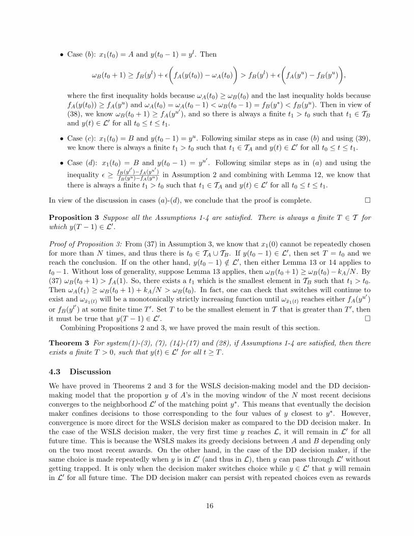
Figure 4: Numerical foraging experiments with pre-defined allocation decision sequence. (a) Snapshotof resource field and robots. (b) Reward for choosing A (explorer) averaged over 100 simulations.

Figure 4 shows the results of simulations with N = 20 robots for a pre-defined decision sequence.All 20 robots are initially exploiters located by a random uniform distribution in a disk of radius0.1L about the center of patch 1. Every decision is to choose A, which is to assign the next robot tobe an explorer. That is, y(0) = 0 and y(kT ) = .05k, k = 1, . . . , 20. The simulation was repeated 100times. Figure 4(a) shows a snapshot of the resource field and foraging robots in one run and Figure4(b) shows the reward fA averaged over all 100 runs. The field parameters are L = 1, a1 = 0.5, σ1 =0.01, a2 = 1.0, and σ2 = 0.2. Exploring robots have speed v = 0.02 and T = 20, γA = 1/2, γB = 3/4,kcom = 0.009 and θ is taken from a uniform distribution in the interval [−π

6 ,π6 ].

The structure of fA in Figure 4 is similar to that of the rising optimum reward structure of Figure1(b). With few explorers, increasing the number of explorers means less resource since explorersabandon patch 1 and search regions that may have lower resource levels. However, with moreexplorers, increasing the number of explorers means greater success at finding the large resourcepeak at patch 2. The negative slope in the reward curve suggests the existence of a matching point,even possibly in the case of less structured decision sequences.

6 Concluding Remarks

In this paper we consider two models for human decision making in the two-alternative forced-choicetask. We provide a formal analysis of matching behavior, a human response strongly supported bypsychology experiments that often corresponds to suboptimal decision strategies. We prove con-vergence to matching for a class of reward curves when the human decision maker is representedby the WSLS model and a deterministic limit of the DD model. We discuss the differences in the

19

convergence of the WSLS decision maker as compared to the DD decision maker. As an applica-tion, we formulate a framework for a human-supervised robotic foraging problem, where the humansupervisor makes decisions, based on a report of performance from the robots, that compare to thekinds of decisions made by the human subject in the psychology experiments, based on a computergenerated reward. The psychology experiments can be viewed as an idealized representation of themore dynamic human-supervised foraging task.

In ongoing work, we are investigating probabilistic models that describe human decision-makingdynamics. This framework will be useful to consider multiple human decision makers in concert withthe results discussed in [15]. We are also exploring how to design an integrated human-robot systemto advantage. We aim to bring to bear the computational power of the robotic system withoutreplacing the human supervisor. As an example, we have been studying adaptive laws for the robotfeedback that use only local information but help the human make optimal decisions.

7 Acknowledgement

We have benefited greatly from discussions with Philip Holmes, Jonathan Cohen, Damon Tomlin,Andrea Nedic, Pat Simen and Deborah Prentice. We thank the anonymous reviewers for theirinsights and constructive comments.

References

[1] R. Murphey and P. M. Pardalos, editors. Cooperative Control and Optimization. Springer, 2002.

[2] V. Kumar, N. Leonard, and A. S. Morse, editors. Cooperative Control. Springer, 2005.

[3] P. Antsaklis and J. Baillieul, editors. IEEE Transactions on Automatic Control: Special Issueon Networked Control Systems, volume 49:9. IEEE, 2004.

[4] P. Antsaklis and J. Baillieul, editors. Proceedings of the IEEE: Special Issue on Technology ofNetworked Control Systems, volume 95:1. IEEE, 2007.

[5] R. Simmons, S. Singh, F. Heger, L. Hiatt, S. Koterba, N. Melchior, and B. Sellner. Human-robotteams for large-scale assembly. In Proc. NASA Science Technology Conference, 2007.

[6] T. Kaupp and A. Makarenko. Measuring human-robot team effectiveness to determine anappropriate autonomy level. In Proc. IEEE Int. Conf. on Robotics and Automation, 2008.

[7] A. Steinfeld, T. Fong, D. Kaber, M. Lewis, J. Scholtz, A. Schultz, and M. Goodrich. Commonmetrics for human-robot interaction. In Proc. Human-Robot Interaction Conference, 2006.

[8] R. Alami, A. Clodic, V. Montreuil, E. A. Sisbot, and R. Chatila. Task planning for human-robotinteraction. In Proc. Joint Conf. on Smart Objects and Ambient Intelligence. ACM, 2005.

[9] J. G. Trafton, N. L. Cassimatis, M. D. Bugajska, D. P. Brock, F. E. Mintz, and A. C. Schultz.Enabling effective human-robot interaction using perspective-taking in robots. IEEE Transac-tions on Systems, Man, and Cybernetics, Part A: Systems and Humans, 35(4):460–470, 2005.

[10] R. Herrnstein. Rational choice theory: necessary but not sufficient. American Psychologist,45:356–367, 1990.

20

[11] P. R. Montague and G. S. Berns. Neural economics and the biological substrates of valuation.Neuron, 36:265–284, 2002.

[12] R. Bogacz, S. M. McClure, J. Li, J. D. Cohen, and P. R. Montague. Short-term memory tracesfor action bias in human reinforcement learning. Brain Research, 1153:111–121, 2007.

[13] J. Li, S. M. McClure, B. King-Casas, and P. R. Montague. Policy adjustment in a dynamiceconomic game. PLoS One, e103:1–11, 2006.

[14] D. M. Egelman, C. Person, and P. R. Montague. A computational role for dopamine deliveryin human decision-making. Journal of Cognitive Neuroscience, 10:623–630, 1998.

[15] A.Nedic, D. Tomlin, P. Holmes, D.A. Prentice, and J.D. Cohen. A simple decision task in asocial context: preliminary experiments and a model. In Proc. of the 47th IEEE Conference onDecision and Control, 2008.

[16] B. Donmez, M. L. Cummings, and H. D. Graham. Auditory decision aiding in supervisorycontrol of multiple unmanned aerial vehicles. Human Factors: The Journal of the HumanFactors and Ergonomics, In press.

[17] K. C. Campbell, Jr. W. W. Cooper, D. P. Greenbaum, and L. A. Wojcik. Modeling distributedhuman decision-making in traffic flow management operations. In 3rd USA/Europe Air TrafficManagement R&D Seminar, Napoli, 2000.

[18] R. Herrnstein. The Matching Law: Papers in Psychology and Economics. Harvard UniversityPress, Cambridge, MA, USA, 1997. Edited by Howard Rachlin and David I. Laibson.

[19] M. Cao, A. Stewart, and N. E. Leonard. Integrating human and robot decision-making dynamicswith feedback: Models and convergence analysis. In Proc. of the 47th IEEE Conference onDecision and Control, 2008.

[20] L. Vu and K. Morgansen. Modeling and analysis of dynamic decision making in sequentialtwo-choice tasks. In Proc. of the 47th IEEE Conference on Decision and Control, 2008.

[21] H. Robbins. Some aspects of the sequential design of experiments. Bulletin of American Math-ematical Society, 58:527–535, 1952.

[22] M. Nowak and K. Sigmund. A strategy of win-stay, lose-shift that outperforms tit-for-tat in thePrisoner’s Dilemma game. Nature, 364:56–58, 1993.

[23] R. Bogacz, E. Brown, J. Moehlis, P. Holmes, and J. D. Cohen. The physics of optimal decisionmaking: A formal analysis of models of performance in two-alternative forced-choice tasks.Psychological Review, 113:700–765, 2006.

[24] B. K. Oksendal. Stochastic Differential Equations: An Introduction with Applications. Springer-Verlag, Berlin, 2003.

[25] P. Simen and J. D. Cohen. Explicit melioration by a neural diffusion model. 2008. Submittedto Brain Research.

[26] P. R. Montague, P. Dayan, and T. J. Sejnowski. A framework for mesencephalic dopaminesystems based on predictive Hebbian learning. Journal of Neuroscience, 16:1936–1947, 1996.

[27] R. S. Sutton and A. G. Barto. Reinforcement learning. MIT Press, Cambridge, MA, 1998.

21

[28] D. Baronov and J. Baillieul. Reactive exploration through following isolines in a potential field.In Proc. of 2007 American Control Conference, pages 2141–2146, 2007.

[29] J. Cortes, S. Martinez, T. Karatas, and F. Bullo. Coverage control for mobile sensing networks.IEEE Transactions on Robotics and Automation, 20:243 – 255, 2004.

[30] P. Ogren, E. Fiorelli, and N.E. Leonard. Cooperative control of mobile sensor networks: Adap-tive gradient climbing in a distributed environment. IEEE Transactions on Automatic Control,49:1292–1302, 2004.

[31] L.A. Giraldeau and T. Caraco. Social foraging theory. Princeton University Press, Princeton,NJ, USA, 2000.

[32] J. Morand-Ferron, L.A. Giraldeau, and L. Lefebvre. Wild carib grackles play a producer-scrounger game. Behavioral Ecology, pages 916–921, July 2007.

[33] C. Baldassano and N. E. Leonard. Explore vs. exploit: Task allocation for multi-robot foraging.Preprint. Available online http://www.princeton.edu/˜ naomi/publications.html, 2009.

22