Convergence, Financial Development, and Policy Analysispeople.bu.edu/miaoj/LMW06.pdf · ation,...
36
Convergence, Financial Development, and Policy Analysis * Justin Yifu Lin † Jianjun Miao ‡ Pengfei Wang § August 13, 2018 Abstract We study the relationship among inflation, economic growth, and financial development in a Schumpeterian overlapping-generations model with credit constraints. In the baseline case money is super-neutral. When the financial development exceeds some critical level, the economy catches up and then converges to the growth rate of the world technology frontier. Otherwise, the economy converges to a poverty trap with a growth rate lower than the frontier and with inflation decreasing with the level of financial development. We then study efficient allocation and identify the sources of inefficiency in a market equilibrium. We show that a particular combination of monetary and fiscal policies can make a market equilibrium attain the efficient allocation. JEL Classification: O11, O23, O31, O33, O38, O42 Keywords: Economic Growth, Innovation, Credit Constraints, Convergence, Policy Analysis, Money, Inflation * We thank Zhengwen Liu for excellent research assistance. † Institute of New Structural Economics, Peking University, 165 Langrunyuan, Haidian, Beijing 100871. Tel: +86-10-62757375. Email: [email protected] ‡ Department of Economics, Boston University, 270 Bay State Road, Boston, MA 02215. Tel.: 617-353-6675. Email: [email protected]. Homepage: http://people.bu.edu/miaoj. § Department of Economics, Hong Kong University of Science and Technology, Clear Water Bay, Hong Kong. Tel: (+852) 2358 7612. Email: [email protected] 1
-
Upload
nguyenduong -
Category
Documents
-
view
214 -
download
0
Transcript of Convergence, Financial Development, and Policy Analysispeople.bu.edu/miaoj/LMW06.pdf · ation,...

Convergence, Financial Development, and Policy Analysis∗
Justin Yifu Lin† Jianjun Miao‡ Pengfei Wang§
August 13, 2018
Abstract
We study the relationship among inflation, economic growth, and financial developmentin a Schumpeterian overlapping-generations model with credit constraints. In the baseline casemoney is super-neutral. When the financial development exceeds some critical level, the economycatches up and then converges to the growth rate of the world technology frontier. Otherwise,the economy converges to a poverty trap with a growth rate lower than the frontier and withinflation decreasing with the level of financial development. We then study efficient allocationand identify the sources of inefficiency in a market equilibrium. We show that a particularcombination of monetary and fiscal policies can make a market equilibrium attain the efficientallocation.
JEL Classification: O11, O23, O31, O33, O38, O42
Keywords: Economic Growth, Innovation, Credit Constraints, Convergence, Policy Analysis,Money, Inflation
∗We thank Zhengwen Liu for excellent research assistance.†Institute of New Structural Economics, Peking University, 165 Langrunyuan, Haidian, Beijing 100871. Tel:
+86-10-62757375. Email: [email protected]‡Department of Economics, Boston University, 270 Bay State Road, Boston, MA 02215. Tel.: 617-353-6675.
Email: [email protected]. Homepage: http://people.bu.edu/miaoj.§Department of Economics, Hong Kong University of Science and Technology, Clear Water Bay, Hong Kong. Tel:
(+852) 2358 7612. Email: [email protected]
1

1 Introduction
The industrial revolution marked a dramatic turning point in the economic progress of nations.
During the nineteenth century, a number of technological leaders in the Western Europe and North
America leapt ahead of the rest of the world, while others lagged behind and became colonies or
semi-colonies of the Western powers. After the WWII, most developing countries obtained political
independence and started their industrialization and modernization process. One might expect
that, with the spread of technology and the advantage of backwardness (Gerschenkron (1962)), the
world should have witnessed convergence in income and living standard. Instead, the post WWII
was a period of continued and accelerated divergence (Pritchett (1997)). According to Maddison
(2008), the per capita GDP in the U.S., the most advanced countries in the 20th century, grew at
an average annual growth rate of 2.1% in the period between 1950 and 2008. While some OECD
and East Asian economies were able to narrow the per capita GDP gap with an annual growth rate
higher than that of the U.S. in the catch up process, most other countries in Latin America, Asia,
and Africa failed to achieve so.1
Why some countries fail to converge in growth rates despite the possibility of technology transfer
has been a puzzle. There are several explanations in the literature.2 In this paper we focus on
the explanation of Aghion, Howitt, and Mayer-Foulkes (henceforth AHM) (2005) and Acemoglu,
Aghion, and Zilibotti (2006) based on a Schumpeterian overlapping-generations (OLG) model of
economic growth with credit constraints.3
We contribute to this literature by analyzing the relationship among growth, inflation, and
financial development. Figure 1 presents the cross-sectional evidence on the sample of 71 countries
over the period 1960-1995.4 Panels A and B show that the average inflation rate is negatively
related to the average per capita GDP growth rate and positively related to the average money
growth rate. Panel C shows that the average inflation rate is negatively related to the average
level of financial development and this relationship vanishes at a high level of financial development
(about 50%). Panel D displays the countries that fail to converge to the world frontier growth rate,
identified by AHM (2005). These countries have a low average level of financial development and
their inflation is negatively related to the average level of financial development.
Motivated by the evidence above, we introduce a monetary authority and a government to
a closed-economy version of the AHM model. We modify this model in several ways. First, we
introduce money by assuming money enters utility (Sidrauski (1967)). This money-in-the-utility
1In the period of 1950-2008, the average per capita GDP growth rates for the whole Latin America, Asia, andAfrica were respectively 1.8%, 1.6%, and 1.2% (Maddison (2008)).
2See Banerjee and Duflo (2005) for a survey.3AHM (2005) provide empirical evidence to support the importance of the credit constraints for convergence or
divergence.4Appendix B presents data description.
2

Figure 1: The average inflation rate, the average per capita GDP growth rate, the average moneygrowth rate, and the average level of financial development, 1960-1995.
approach can be microfounded in several ways once one takes into account the role of medium of
exchange (McCallum (1983)). Although money can be valued in the OLG model as a store of value
(Samuelson (1958)), the equilibrium net nominal interest rate is zero and hence one cannot analyze
monetary policy in terms of interest rate rules. Our modeling of money avoids this issue.5 Second,
we introduce intra-generational heterogeneity so that there are savers and borrowers (entrepreneurs)
in each period. We can then endogenize the nominal interest rate in a credit market and study how
credit market imperfections affect interest rates. Third, we assume savers are risk averse so that
we can derive their consumption and portfolio choices. In each period a young saver must choose
optimal consumption, money holdings, and saving in terms of nominal bonds.
We show that the market equilibrium in our model can be summarized by a system of four
nonlinear difference equations for four sequences of variables: the nominal interest rate, the inflation
rate, the normalized R&D investment, and the proximity to the technological frontier. For this
equilibrium system, monetary policy is modeled by a money supply rule. If one uses an interest
rate rule as in the dynamic new Keynesian literature (Woodford (2003)), then money supply is
endogenous and the nominal interest rate is replaced by the money growth rate in the equilibrium
system. Due to the complexity of our model, we cannot reduce this system to a scalar one for
5Another approach is to introduce a cash-in-advance constraint.
3

the proximity variable alone as in the AHM model. However we are still able to provide a full
characterization of the steady state along a balanced growth path, which is consistent with the
evidence presented in Figure 1.
It turns out that how money supply is introduced to the economy is critical for how money
affects the equilibrium allocation and long-run growth. We first show that, if money increments
are transferred to the old agents in an amount proportional to their pre-transfer money holdings,
then money is super-neutral in the sense that monetary policy does not affect long-run growth and
the equilibrium allocation along a balanced growth path.6 This result dates back to Lucas’s (1972)
model, in which there is no endogenous growth. The intuition is that the demand for money and
saving depends on the ratio of the nominal interest rate and the money growth rate and hence the
real interest rate in the long run. Thus only real variables are determined in the steady state.
We show that there are three dynamic patterns as in the AHM model with the difference that
our model incorporates inflation:
1. When the credit market is perfect so that the credit constraint does not bind, the econ-
omy converges to the world frontier growth rate and there is no marginal effect of financial
development.
2. When the credit constraint binds, but is not tight enough, the economy converges to the
world frontier growth rate with a level effect of financial development.
3. When the credit constraint is sufficiently tight, there is divergence in growth rates with a
growth effect of financial development. In this case the economy enters an equilibrium with
poverty trap.
Using numerical examples, we find that the steady states for all these three cases are saddle
points. For any given initial value of the proximity to the frontier, there exists a unique saddle path
such that the economy will transition to the steady state. For the first two cases, the transition
paths display the feature of the advantage of backwardness (Gerschenkron (1962)). Moreover, the
inflation rate rises during the transition. But for the third case, the economy exhibits the feature
of the disadvantage of backwardness and falls into the poverty trap with low economic growth,
low innovation, and high inflation. The inflation rate declines during the transition. Moreover,
the long-run rate of productivity growth increases with financial development and the long-run
inflation rate decreases with financial development.
Next we study efficient allocation. Suppose that there is a social planner who maximizes the
sum of discounted utilities of all agents in the present and future generations. We derive the
efficient allocation and long-run growth rate. By comparing with the efficient allocation, we find
6Money growth has a short-run effect on the transition path.
4

there are four sources of inefficiency in a market equilibrium. First, there is monopoly inefficiency
in the production of intermediate goods. The resulting price distortion generates an inefficiently
low level of final net output when taken the innovation rate as given. Second, the private return
to innovation ignores the dynamic externality or spillover effect of technology. Third, the credit
market imperfection prevents innovators to obtain necessary funds for R&D. Finally, the OLG
framework itself may cause dynamic inefficiency.
Can a combination of monetary and fiscal policies correct the preceding inefficiencies and make
the market equilibrium attain the efficient allocation? We show that when money increments
are transferred to the entrepreneur, money is not super-neutral and there is a particular nominal
interest rate such that the market equilibrium can achieve innovation efficiency, but it cannot
achieve output and consumption efficiency. The intuition is that money growth is like an inflation
tax and there is a wealth effect when the tax is not proportionally distributed to the agents according
to their pre-transfer money holdings. Money affects the real economy through the redistribution
channel. We then introduce fiscal policies to attain the efficient allocation. We find different
policies are needed in different development stages. When the economy faces severe credit market
imperfections, the government should try to loosen credit constraints by ensuring better contract
enforcements or better monitoring of borrowers. For example, the government can make direct
lending to entrepreneurs financed by lump-sum taxes on savers. When the government has better
monitoring technologies than private agents, the credit constraints can be overcome. The economy
can then avoid the equilibrium with poverty traps.
Our paper is related to several strands of literature. First, it is related to the literature on
poverty traps and convergence or divergence in economies with credit market imperfections (e.g.,
Banerjee and Newman (1993), Galor and Zeira (1993), Howitt (2000), Mookherjee and Ray (2001),
Azariadis and Stachurski (2005), Howitt and Mayer-Foulkes (2005), Aghion, Howitt, and Mayer-
Foulkes (2005) and Acemoglu, Aghion, and Zilibotti (2006)). As pointed out by Azariadis and
Stachurski (2005) in their survey, this literature typically studies models of self-reinforcing mecha-
nisms that cause poverty to persist. In these models there is no technical progress and therefore no
positive long-run growth. As discussed earlier, our paper is most closely related to Aghion, Howitt,
and Mayer-Foulkes (2005) and Acemoglu, Aghion, and Zilibotti (2006), which incorporate long-run
growth. Unlike these two papers, we introduce money, endogenize interest rates, and provide a
policy analysis. Howitt and Mayer-Foulkes (2005) also derive three convergence patterns analogous
to those in our paper, but the disadvantage of backwardness that prevents convergence in that
paper arises from low levels of human capital rather than from credit-market imperfections.
Second, our paper is related to the literature that analyzes the effects of financial constraints or
financial intermediation on long-run growth. Early contributions include Greenwood and Jovanovic
(1990), Bencivenga and Smith (1991), and King and Levine (1993). None of these papers studies
5

technology transfer and the associated policy issues which are our focus.
Third, our paper is related to the literature on the relation between money and growth. Recent
papers include Gomme (1991), Marquis and Reffett (1994), Chu and Cozzi (2014), Jones and
Manuelli (1995), Miao and Xie (2013), and Chu et al. (2017), among others. These papers typically
introduce money via cash-in-advance constraints in infinite-horizon models, which do not feature
poverty traps. By contrast, we follow the money-in-the-utility function approach of McCallum
(1983) and Abel (1987) in the OLG framework. Our focus is on how monetary and fiscal policies
can attain efficient allocation and avoid poverty traps.
2 The Model
We consider a monetary overlapping generations model of a closed economy based on Aghion,
Howitt, and Mayer-Foulkes (2005) and Acemoglu, Aghion, and Zilibotti (2006). Time is discrete
and runs forever. Time is denoted by t = 1, 2, . . . . Each generation has a unit measure of identical
entrepreneurs and a unit measure of identical savers. Each agent lives for two periods. Only
entrepreneurs can conduct innovation, but they face borrowing constraints. Savers lend funds to
entrepreneurs, but they cannot innovate. As a benchmark, we follow Lucas (1972) and assume that
the government (or central bank) directly transfers money to all agents and the monetary transfer
is proportional to each agent’s pre-transfer money holdings.
2.1 Production
All agents work for the producers who combine labor and a continuum of specialized intermediate
goods to produce a general good according to the production function,
Zt = L1−αt
∫ 1
0At (i)1−α xt (i)α di, (1)
where Lt is labor demand, xt (i) is the input of the latest version of intermediate good i, and At (i)
is the productivity parameter associated with it. The general good is used for consumption, as an
input to R&D and also as an input to the production of intermediate goods. The general good is
produced under perfect competition. Suppose that the aggregate labor supply is normalized to one
and the real price of the general good is also normalized to one. Then the equilibrium real price of
each intermediate good equals its marginal product:
pt (i) = α
(xt (i)
At (i)
)α−1
. (2)
For each intermediate good i there is one entrepreneur born each period t who is capable of
producing an innovation for the next period. If he succeeds in innovating, then he will be the ith
6

incumbent in period t + 1. Let µt (i) be the probability that he succeeds. Then the technology
evolves according to
At+1 (i) =
{At+1 with probability µt (i)At (i) with probability 1− µt (i)
,
where At+1 is the world frontier technology, which grows at the exogenously given constant rate
g > 0. That a successful innovator gets to implement At+1 is a manifestation of technology transfer
in the sense that domestic R&D makes use of ideas developed elsewhere in the world. If an
innovation fails, the intermediate good sector i uses the technology in the previous period.
In each intermediate good sector where an innovation has just occurred, the incumbent can
produce one unit of the intermediate good using one unit of the general good as the only input.
In each intermediate sector there are an unlimited number of people capable of producing copies
of the latest generation of that intermediate good at a unit cost of χ > 1. The fact that χ > 1
implies that the fringe is less productive than the incumbent producer. The parameter χ captures
technological factors as well as government regulation affecting entry. A higher χ corresponds to
a less competitive market. So in sectors where an innovation has just occurred, the incumbent
will be the sole producer, at a price equal to the unit cost of the competitive fringe, whereas in
noninnovating sectors where the most recent incumbent is dead, production will take place under
perfect competition with a price equal to the unit cost of each producer. In either event the price
will be χ, and according to the demand function (2) the quantity demanded will be
xt (i) =
(α
χ
) 11−α
At (i) . (3)
It follows that an unsuccessful innovator will earn zero profits next period, whereas the real
profit of a successful incumbent will be
Ψt (i) = pt (i)xt (i)− xt (i) = (χ− 1)
(α
χ
) 11−α
At ≡ ψAt,
where ψ represents the normalized profit:
ψ = (χ− 1)
(α
χ
) 11−α
.
2.2 Entrepreneurs
An entrepreneur born in period t ≥ 1 is endowed with λ ∈ (0, 1) units of labor when young and
supplies labor inelasically to the general good producers. He derives utility from consumption cet+1
when old according to
β log(Etc
et+1
),
7

where β ∈ (0, 1) is the subjective discount factor. This utility function is an increasing transfor-
mation of a risk-neutral utility function. We will see the role of the log transformation in Section
4.
An innovation costs Nt units of general good in period t. The young entrepreneur receives
labor income λwt, which may not be sufficient to cover the innovation cost Nt. Suppose that the
entrepreneur borrows Bt dollars at the nominal interest rate Rft between periods t and t+ 1 from
the savers so that
Nt =BtPt
+ λwt, (4)
where Pt denotes the price level and wt is the real wage rate.
We follow Aghion, Banerjee, and Piketty (1999) and Aghion, Howitt, and Mayer-Foulkes (2005)
to model financial market imperfections. Suppose that the entrepreneur can hide a successful
innovation at a real cost κNt so that he can avoid repaying debt. The parameter κ ∈ (0, 1)
reflects the degree of financial development. A higher value of κ means that it is more costly for
the entrepreneur to misbehave. It measures the degree of creditor protection. To implement the
contract without default, the entrepreneur faces an incentive constraint
β
(µtψAt+1 −Rft
BtPt+1
)≥ βµtψAt+1 − κNt,
where the expression on the left-hand side of the inequality is the discounted expected consumption
if the entrepreneur behaves and the expression on the right-hand side is the discounted expected
consumption if he is dishonest. Simplifying yields the borrowing constraint
BtPt≤ κNt
βRft/Πt+1, (5)
where Πt+1 = Pt+1/Pt denotes the inflation rate. By (4) this constraint is equivalent to
Nt ≤βRft/Πt+1
βRft/Πt+1 − κλwt (6)
for βRft/Πt+1 > κ. Thus R&D investment is limited by a multiple of the entrepreneur’s net worth
λwt. This multiple is called the credit multiplier by AHM and increases with κ, but decreases with
the real interest rate.
Suppose that
Nt = Φ(µt)At+1,
where the function Φ is twice continuously differentiable and satisfies Φ(0) = 0 and Φ′ > 0 and
Φ′′> 0. The factor At+1 reflects the “fishing-out” effect: the further ahead the frontier moves, the
more difficult it is to innovate. This effect is important to have a balanced growth path. We can
also rewrite the preceding equation as
µt = F(Nt/At+1
), (7)
8

where F = Φ−1 satisfies F (0) = 0, F ′ > 0, and F ′′ < 0.
The entrepreneur’s expected consumption is given by
Etcet+1 = µtψAt+1 −
RftBtPt+1
= F
(Nt
At+1
)ψAt+1 −
RftPtPt+1
(Nt − λwt) .
The entrepreneur’s objective is to solve the following problem
maxNt
F(Nt/At+1
)ψAt+1 −
RftPtPt+1
(Nt − λwt)
subject to (6). When the credit constraint (6) does not bind, the first-order condition is given by
F ′(
Nt
At+1
)ψ =
RftΠt+1
, (8)
where Πt+1 = Pt+1/Pt denotes the inflation rate. This condition says that the expected marginal
return to R&D is equal to the real interest rate.
The initial old entrepreneur at time t does not have labor income and hence does not conduct
innovation. We assume that he simply consumes his money endowment M e0 and the government
proportional transfer M e0z1.
2.3 Savers
A saver born at time t ≥ 1 is endowed with 1 − λ units of labor when young and supplies labor
inelastically to the general good producers. He has the utility function
log(cyt ) + β log(cot+1) + γ log (Mt/Pt) , γ > 0,
where β is the discount factor, cyt (cot+1) denotes consumption at time t (t + 1) when the saver
is young (old), Mt denotes money holdings chosen in period t. He faces the following budget
constraints
cyt +StPt
+Mt
Pt= (1− λ)wt,
cot+1 =StRftPt+1
+Mt (1 + zt+1)
Pt+1,
where St denotes saving and zt+1 ≥ 0 denotes the proportional rate of the monetary transfer from
the government. Note that the above utility specification does not have a satiation level of real
balances as in Friedman (1969).
The first-order conditions give1
cyt= β
1
cot+1
PtPt+1
Rft,
and1
cyt=
γ
Mt/Pt+
β
cot+1
Pt(1 + zt+1)
Pt+1.
9

Using these conditions and the budget constraints, we can derive that
cyt =(1− λ)wt1 + β + γ
, (9)
Mt
Pt=
γ(1− λ)wt1 + β + γ
1
1− (1 + zt+1) /Rft, (10)
StPt
=(1− λ)wt1 + β + γ
[β − γ
Rft/ (1 + zt+1)− 1
]. (11)
Thus, consumption, the money demand, and the saving demand are all proportional to the saver’s
real wealth (1− λ)wt. Moreover the money demand decreases with Rft/ (1 + zt+1) and the saving
demand increases with Rft/ (1 + zt+1) . This property is important for the long-run super-neutrality
of money because Rft/ (1 + zt+1) is proportional to the real interest rate in the steady state, which
is independent of the inflation rate.
We assume that
Rft > (1 + zt+1)
(1 +
γ
β
). (12)
This assumption ensures that the money demand Mt/Pt > 0 and the saving demand St/Pt > 0.
The initial old saver is endowed with money holdings M s0 and derives utility according log (co1) ,
where
co1 =M s
0 (1 + z1)
P1.
2.4 Competitive Equilibrium
Define the aggregate technology as
At =
∫At (i) di.
In equilibrium the probability of innovation will be the same in each sector: µt (i) = µt for all i.
Thus average productivity evolves according to
At+1 = µtAt+1 + (1− µt)At. (13)
Define the normalized productivity as at = At/At. Normalized productivity is an inverse measure of
the country’s distance to the technological frontier, or its technology gap. It describes the proximity
to the technological frontier and satisfies the dynamics
at+1 = µt +1− µt1 + g
at. (14)
Equation (13) implies that
At+1 −AtAt
= µt
(1 + g
at− 1
).
Thus there is an advantage of backwardness (Gerschenkron (1962)) in the sense that the further
the country is behind the frontier, the faster the country grows. On the other hand, the country’s
10

growth rate also depends on innovation µt. More innovation allows more firms to adopt the frontier
technology and hence enhancing growth. Thus the net effect depends on both at and µt. Here µt or
R&D investment is like the role of human capital that determines a country’s “absorptive capacity”
(Nelson and Phelps (1966)).
In equilibrium Lt = 1. We then use (1), (2), and pt (i) = χ to derive aggregate output of the
general good
Zt = ζAt, where ζ ≡(α
χ
) α1−α
.
The wage rate is given by
wt = (1− α)Zt = (1− α) ζAt. (15)
The equilibrium interest rate Rft and the price level Pt are determined by the market-clearing
conditions for credit and money: Bt = St and Mt = (1 + zt)Mt−1 for t ≥ 1, where zt is the money
growth rate controlled by the central bank and M0 = M s0 +M e
0 is given.
By (4), (11), and the market-clearing condition Bt = St, we have
Nt − λwt =(1− λ)wt1 + β + γ
[β − γ(1 + zt+1)
Rft − (1 + zt+1)
]. (16)
Value added in the general sector is wage income, whereas value added in the intermediate
sectors is profit income. Total GDP is the sum of value added in all sectors:
Yt = wt + µt−1ψAt = (1− α) ζAt + µt−1ψAt. (17)
3 Equilibrium Balanced Growth Paths
In this section we solve for competitive equilibrium and derive equilibrium balanced growth path.
3.1 Perfect Credit Markets
Suppose that the credit constraint (6) does not bind so that the credit market is perfect. It follows
from (8) that the optimal innovation is determined by the condition
F ′(nt)ψ =RftΠt+1
, (18)
where we define nt = Nt/At+1. We can rewrite (14) as
at+1 = F (nt) +1− F (nt)
1 + gat. (19)
Conjecture that the economy will grow at the rate of the world technology frontier along a
balanced growth path so that At+1 = (1 + g)At. Using (10) to compute the ratio Mt+1/Mt and
then imposing the money market-clearing condition Mt+1 = Mt (1 + zt+1), we obtain
(1 + zt+1)PtPt+1
=Mt+1/Pt+1
Mt/Pt=
wt+1
1−(1+zt+2)/Rft+1
wt1−(1+zt+1)/Rft
.
11

Using (15), at = At/At, and At+1 = (1 + g)At, we can simplify the preceding equation as
Πt+1 = (1 + zt+1)1− (1 + zt+2) /Rft+1
1− (1 + zt+1) /Rft
atat+1 (1 + g)
. (20)
Thus the inflation rate is determined by money demand and money supply, which in turn are
determined by the nominal interest rate, the growth rate of domestic productivity, and the growth
rate of money supply. Using nt = Nt/At+1, (15), and (16), we derive that
nt =(1− α) ζat
1 + g
[λ+
(1− λ)
1 + β + γ
(β − γ(1 + zt+1)
Rft − (1 + zt+1)
)]. (21)
Now the competitive equilibrium under perfect credit markets can be summarized by a system
of four difference equations (18), (19), (20), and (21) for four sequences {Rft}, {at} , {Πt+1}, and
{nt} such that (12) and (6) are satisfied.
We first study the balanced growth path in the steady state. We use a variable without time
subscript to denote its steady state value. It follows from (20) that the steady-state inflation is
given by
Π =1 + z
1 + g, (22)
which increases with the money growth rate, but decreases with the productivity growth rate. We
then obtain a system of three equations
n =(1− α) ζa
1 + g
{λ+
(1− λ)
1 + β + γ
[β − γ
Rf/ (1 + z)− 1
]}, (23)
Rf =1 + z
1 + gF ′(n)ψ, (24)
a =(1 + g)F (n)
g + F (n), (25)
to determine three variables n, Rf , and a.
From equations (23), (24), and (25), we can show that n is determined by the equation
n =(1− α) ζF (n)
g + F (n)
{λ+
(1− λ)
1 + β + γ
[β − γ
F ′(n)ψ/ (1 + g)− 1
]}.
Equivalently, µ is determined by the equation
Φ′ (µ) =ψ
Rf/Π, (26)
where
RfΠ
= (1 + g)
1 +γ
β −[
Φ(µ)(g+µ)(1−α)ζµ − λ
]1+β+γ
1−λ
.
We can check that the real interest rate Rf/Π is decreasing in µ and Φ′ (µ) is increasing in µ.
Assuming that
Φ′ (0) <ψ
1 + g
1 +γ
β −[
Φ′(0)g(1−α)ζ − λ
]1+β+γ
1−λ
−1
, (27)
12

and
Φ′ (1) >ψ
1 + g
1 +γ
β −[
Φ(1)(g+1)(1−α)ζ − λ
]1+β+γ
1−λ
−1
, (28)
we use the intermediate value theorem to deduce that there is a unique solution µ∗ ∈ (0, 1) to (26).7
The associated R&D investment is given by n∗ = Φ (µ∗) and hence R∗f and a∗ are determined by
(24) and (25). We also assume that the condition
R∗f1 + z
> 1 +γ
β(29)
is satisfied so that (12) holds along the balanced growth path. We will verify later that this condition
is indeed satisfied.
Using (23) and (15), we can rewrite the credit constraint (6) along a balanced growth path as
n
(βRf
Π− κ)≤βRf
Π
λ (1− α) ζa
1 + g.
The critical value of κ such that the credit constraint just binds in equilibrium is given by
κ∗ =βR∗f
Π
[1− λ (1− α) ζa∗
n∗ (1 + g)
]. (30)
When κ > κ∗, the credit constraint does not bind. It follows from (26) that money supply does not
affect the equilibrium innovation rate µ∗. An increase in the money growth rate raises the nominal
interest rate one for one and hence does not affect savings. Thus the supply of funds for innovation
does not depend on monetary policy. We summarize the result below.
Proposition 1 Suppose that the monetary transfer is given to the old generation only in a quantity
proportional to the pre-transfer money holdings of each. Let conditions (27) and (28) hold. If
κ ≥ κ∗, where κ∗ satisfies (30), then there is a unique steady state with µ∗ ∈ (0, 1) such that the
credit constraint does not bind and the productivity grows at the rate g. In this steady state money
is super-neutral in the sense that the steady-state real quantities are independent of money growth
rate z. They are also independent of κ.
Since µ∗ ∈ (0, 1) , the economy can never reach the world technology frontier in that a∗ ∈ (0, 1) .
For the economy to reach the frontier, we must have condition (28) hold with equality so that
µ∗ = a∗ = 1. This case can happen when innovation profits are sufficiently large, i.e., ψ is sufficiently
large.
We use a numerical example to illustrate the transition dynamics. As in AHM (2006), we set
Φ (µ) = φµ + δ2µ
2 and F (n) = 1δ
(√2nδ + φ2 − φ
). We choose parameter values as α = 0.8,
χ = 1.15, φ = 0.0134, δ = 0.2604, λ = 0.01, g = 0.04, β = 0.96, and γ = 0.017. We assume that
7We do not consider the knife-edge case of boundary solutions.
13

money supply grows at a constant rate z = 0.06. Our simple two-period lived OLG model cannot
be calibrated to confront with data. We use our numerical example to illustrate the working of our
model. We find that the critical value κ∗ = 0.678. We choose an arbitrary κ > κ∗. Then the steady
state values are given by R∗f = 1.08, Π∗ = 1.0192, a∗ = 0.5, µ∗ = 0.037, n∗ = 0.0007. Moreover,
the GDP Yt normalized by At is equal to 0.024. The steady state is a saddle point. Only at is a
predetermined variable. Figure 2 illustrates the transition dynamics for the case of perfect credit
markets when the economy starts at a1 = 0.3. We find that µt, at, and Πt gradually increases to
their steady state values, but Rft decreases to its steady state value. Given that we take the the
money growth rate fixed, the inflation rate moves inversely with the growth rate of productivity.
The transition path illustrates the advantage of backwardness. When the economy initially falls
behind the world frontier, both its technology and innovation grow faster. Thus its GDP also grows
faster. They eventually catch up with the growth rate of the world frontier.
0 50 1000.032
0.034
0.036
0.038t
0 50 1000.96
0.98
1
1.02t+1
0 50 1000.3
0.35
0.4
0.45
0.5a
t
0 50 1001.08
1.0802
1.0804
1.0806
1.0808R
ft
0 50 1000.04
0.06
0.08
0.1A
t+1/A
t-1
0 50 1001.04
1.06
1.08
1.1
1.12R
ft/
t+1
Figure 2: Transition dynamics for the case of perfect credit markets.
The steady-state proximity to frontier a∗ depends on the preference and technology parameters.
A crucial parameter is the marginal cost of innovation φ given the quadratic specification of Φ.
By (26), a higher φ raises the marginal cost and reduces the marginal benefit by reducing the
real interest rate, thereby reducing the innovation rate µ∗. This causes the economy’s absorptive
capacity to be smaller so that a∗ is smaller.
14

3.2 Binding Credit Constraints
Suppose that the credit constraint (6) binds. Using (16) and (6) we obtain
wt
{λ+
(1− λ)
1 + β + γ
[β − γ(1 + zt+1)
Rft − (1 + zt+1)
]}=
βRft/Πt+1
βRft/Πt+1 − κλwt. (31)
We also require that
F ′ (nt)ψ >RftΠt+1
. (32)
Now the equilibrium system consists of equations (19), (20), (21), and (31) for four sequences
{Rft}, {at} , {Πt+1}, and {nt} such that (12) and (32) hold.
In the steady state the equilibrium system becomes (22), (23), (25), and the following equation
λ+1− λ
1 + β + γ
[β − γ
Rf/ (1 + z)− 1
]︸ ︷︷ ︸
supply
=λβRf/Π
βRf/Π− κ︸ ︷︷ ︸limit
. (33)
The expression on the left-hand side of equation (33) is increasing in Rf and the expression on the
right-hand side is decreasing in Rf . Thus there is a unique solution for Rf to the equation above
such thatRf
1 + z> max
{1 +
γ
β,
κ
β (1 + g)
}. (34)
Let R∗∗f denote the solution. Using equations (23), (25) and (33), we derive that
n =λ (1− α) ζF (n)
g + F (n)
βR∗∗f /Π
βR∗∗f /Π− κ.
We can equivalently rewrite this equation in terms of µ as
Φ (µ) (g + µ) =(1− α) ζλβR∗∗f /Π
βR∗∗f /Π− κµ. (35)
Assume that
Φ′ (0) g <(1− α) ζλβR∗∗f /Π
βR∗∗f /Π− κ< Φ (1) (g + 1) . (36)
Then it follows from the intermediate value theorem that there is a unique solution, denoted
by µ∗∗ ∈ (0, 1) , to the equation (35). The corresponding R&D investment level is denoted by
n∗∗ = Φ (µ∗∗) .
Define the critical values κ∗∗ and κ for κ such that
Φ′ (0) g =(1− α) ζλβR∗∗f /Π
βR∗∗f /Π− κ∗∗,
(1− α) ζλβR∗∗f /Π
βR∗∗f /Π− κ= Φ (1) (g + 1) .
15

where R∗∗f is the solution to equation (33) and is a function of κ. We can verify that the expression
R∗∗f /Π
R∗∗f /Π− κ
increases with κ along the supply curve in Figure 3. Thus the values κ∗∗ and κ are unique.
We summarize the result below.
Proposition 2 Suppose that the monetary transfer is given to the old generation only in a quantity
proportional to the pre-transfer money holdings of each. If κ∗∗ < κ < min {κ∗, κ} , then there is
a unique steady state such that the credit constraint binds and the productivity grows at the rate
g. In this steady state we have µ∗∗ ∈ (0, 1) , 0 < n∗∗ < n∗, and R∗∗f < R∗f . Moreover, money is
super-neutral, and n∗∗, µ∗∗, and R∗∗f increase with κ.
We use Figure 3 to illustrate the determination of the steady-state nominal interest rate. The
curve labeled “Supply” describes the supply of funds normalized by the wage rate, which is given
by the expression on the left-hand side of equation (33). This curve increases with the nominal
interest rate Rf . The curve labeled “Demand” describes the demand for funds normalized by the
wage rate, which is given byNt
wt=
n(1−α)ζF (n)g+F (n)
. (Demand)
It increases with n. Using (24) to substitute for n, we can show that the above expression decreases
with Rf . The curves labeled “Limit κ > κ∗” and “Limit κ < κ∗” describe the borrowing limits
normalized by the wage rate for κ > κ∗ and κ < κ∗, respectively, which are given by the expression
on the right-hand side of equation (33). This expression decreases with Rf .
When κ > κ∗, the equilibrium nominal interest rate R*f is determined by the intersection of the
demand curve and the supply curve. In this case the credit constraint does not bind and a change
in κ does not affect equilibrium. When κ < κ∗, the credit constraint binds so that the equilibrium
nominal interest rate R∗∗f is determined by the intersection of the supply curve and the borrowing
limit curve. From the figure we can see that R∗∗f < R∗f and an increase in κ raises R∗∗f . However
the change in κ does not have a growth effect.
For a numerical illustration, we choose the same parameter values as in Section 3.1 except that
we set κ = 0.5. Then the credit constraint binds. We find the steady state values R∗∗f = 1.0796,
Π∗∗ = 1.0192, a∗∗ = 0.327, µ∗∗ = 0.018, and n∗∗ = 0.0003. The normalized GDP is equal to 0.016.
Compared to the case of perfect credit markets, credit market imperfections enlarges the distance
to the frontier even though grow rates are the same in that a∗∗ < a∗, µ∗∗ < µ∗, n∗∗ < n∗, and
normalized GDP are all smaller. We find that the steady state is also a saddle point. Figure 4
illustrates the transition dynamics, which also display the advantage of backwardness.
16

Limit � > �∗
Demand
Supply
Limit � < �∗
��∗∗ ��
∗
Figure 3: Determination of the steady-state equilibrium nominal interest rates. The curves labeled“Supply” and “Demand” describe the supply of and demand for funds normalized by the wage rate,respectively. The curves labeled “Limit κ > κ∗” and “Limit κ > κ∗” describe the borrowing limitsnormalized by the wage rate for κ > κ∗ and κ < κ∗, respectively.
0 200 4000.005
0.01
0.015
0.02t
0 200 4001
1.005
1.01
1.015
1.02t+1
0 200 4000.1
0.2
0.3
0.4a
t
0 200 4001.079545
1.07955
1.079555
1.07956
1.079565R
ft
0 200 4000.04
0.045
0.05
0.055
0.06A
t+1/A
t-1
0 200 4001.05
1.06
1.07
1.08R
ft/
t+1
Figure 4: Transition dynamics for the case of binding credit constraints.
17

3.3 Poverty Trap
Since Φ (0) = 0 by assumption, we deduce that there is another solution to (35) denoted by µ = 0.
In this case the corresponding a = n = 0. The economy enters a poverty trap. When κ is sufficiently
small, condition (36) is violated. Then the only steady state equilibrium is the poverty trap. In the
poverty trap the economy still grows but at a rate lower than g. In Proposition 3 below we show
that
limt→∞
At+1
At= (1 + g) lim
t→∞
at+1
at= F ′ (0)
(1− α) ζλβRf/Π
βRf/Π− κ+ 1,
where Rf is the steady-state nominal interest rate. By (20) the steady-state inflation rate satisfies
Π =1 + z
F ′ (0)(1−α)ζλβRf/ΠβRf/Π−κ + 1
, (37)
instead of equation (22). The poverty-trap steady state is characterized by a system of two equations
(33) and (37) for two variables Rf and Π. In the appendix we prove that there is a unique solution,
denoted by Rf and Π.
Proposition 3 Suppose that the monetary transfer is given to the old generation only in a quantity
proportional to the pre-transfer money holdings of each. If 0 < κ < κ∗∗, then there is a unique
steady-state equilibrium, which enters the poverty trap with µ = a = n = 0. Money is super-neutral.
The steady-state productivity growth rate is given by
limt→∞
At+1
At= F ′ (0)
(1− α) ζλβRf/Π
βRf/Π− κ+ 1,
which is between 0 and 1 + g and increases with κ ∈ (0, κ∗∗) . The steady-state inflation rate Π >
(1 + z) / (1 + g) and decreases with κ ∈ (0, κ∗∗) .
To illustrate this proposition numerically, we use the same parameter values as in Section 3.1
except that we set κ = 0.1. We then find the poverty trap equilibrium with the steady-state values
Rf = 1.0792 and Π = 1.0205. In the steady-state, the normalized GDP is equal to 0 and the
technology growth rate is 1.0387. The steady-state inflation rate is higher than the two cases
studied in Sections 3.1 and 3.2. We also find the poverty-trap steady state is a saddle point.
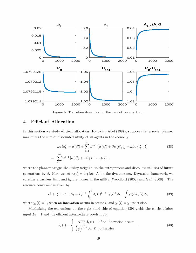
Figure 5 illustrates the transition dynamics when the economy starts at a1 = 0.5. It shows that
the economy falls further behind the world frontier. Both at and µt decrease to zero. The inflation
rate Πt and the nominal interest rate Rft also decrease to their steady-state values, but the real
interest rate Rft/Πt+1 increases to its steady-state value. The growth rate of productivity increases
to a level lower than the world frontier. The economy falls into a poverty trap with low economic
growth and high inflation. Thus there is a disadvantage of backwardness when the level financial
development is extremely low.
18
0 1000 20000
0.005
0.01
0.015
0.02t
0 1000 20000
0.2
0.4
0.6a
t
0 1000 20000.01
0.02
0.03
0.04A
t+1/A
t-1
0 1000 20001.079211
1.0792115
1.079212
1.0792125R
ft
0 1000 20001.02
1.03
1.04
1.05t+1
0 1000 20001.03
1.04
1.05
1.06R
ft/
t+1
Figure 5: Transition dynamics for the case of poverty trap.
4 Efficient Allocation
In this section we study efficient allocation. Following Abel (1987), suppose that a social planner
maximizes the sum of discounted utility of all agents in the economy
ωu (ce1) + u (co1) +∞∑t=1
βt−1[u (cyt ) + βu
(cot+1
)+ ωβu
(cet+1
)](38)
=
∞∑t=1
βt−1 [u (cyt ) + u (cot ) + ωu (cet )] ,
where the planner assigns the utility weight ω to the entrepreneur and discounts utilities of future
generations by β. Here we set u (c) = log (c) . As in the dynamic new Keynesian framework, we
consider a cashless limit and ignore money in the utility (Woodford (2003) and Gali (2008)). The
resource constraint is given by
cyt + cot + cet +Nt = L1−αt
∫ 1
0At (i)1−α xt (i)α di−
∫χt(i)xt (i) di, (39)
where χt(i) = 1, when an innovation occurs in sector i, and χt(i) = χ, otherwise.
Maximizing the expressions on the right-hand side of equation (39) yields the efficient labor
input Lt = 1 and the efficient intermediate goods input
xt (i) =
α1
1−αAt (i) if an innovation occurs(αχ
) 11−α
At (i) otherwise. (40)
19
We can then compute the GDP (net output):
Y et =
∫ 1
0At (i)1−α xt (i)α di−
∫χt(i)xt (i) di
=
(1
α− 1
)[α
11−αµt−1At + (1− µt−1)
(α
χ
) 11−α
χAt−1
]. (41)
The resource constraint (39) becomes
cyt + cot + cet +Nt = Y et . (42)
where µ0 = 0 and A0 is exogenously given.
Now the planner’s problem is to maximize (38) subject to (7), (13), and (42). Let βtΛt and
βtΛtqt be the Lagrange multipliers associated with (42) and (13), respectively. The variable qt
represents the shadow value of the technology At+1. The first-order conditions are given by
ωu′ (cet ) = u′ (cot ) = u′ (cyt ) = Λt,
Λt = βΛt+1(1
α− 1)
[α
11−α At+1 −
(α
χ
) 11−α
χAt
]F ′(Nt/At+1
)At+1
+Λtqt[At+1 −At]F ′(Nt/At+1
)At+1
,
Λtqt = β(1− µt+1)Λt+1qt+1 + β2Λt+2(1− µt+1)(1
α− 1)
(α
χ
) 11−α
χ.
We can immediately derive that
cet = ωcyt = ωcot . (43)
The efficiency condition for Nt says that the marginal social cost of R&D Λt must be equal to the
marginal social benefit, which reflects the fact that an increase in Nt raises the current innovation
probability µt, which in turn raises the domestic productivity. Rising productivity has two benefits.
First, it raises profits. Second, it causes the domestic productivity to be closer to the world frontier.
The efficiency condition for At+1 is similar to an asset pricing equation for capital. It says that
the shadow price of technology is equal to the discounted present value of future dividends, which
are equal to the profits contributed by domestic technology alone when no innovation occurs. We
emphasize that innovation has a positive long-lasting externality effect because it raises all future
productivities.
Since At+1/At = 1 + g, we conjecture that, on the balanced growth path, at = At/At, µt,
Nt/At+1 = nt, and qt are constant over time, but cyt , cot , and cet all grow at the rate g. We then have
q =β
1 + g(1− µ)q +
(β
1 + g
)2
(1− µ)(1
α− 1)
(α
χ
) 11−α
χ,
20

and1
F ′ (n)= β
1
1 + g(
1
α− 1)
[α
11−α −
(α
χ
) 11−α
χa
1 + g
]+ q
[1− a
1 + g
].
Equation (13) implies
a =F (n) (1 + g)
g + F (n). (44)
Using the above three equations we can derive
1
F ′ (n)=
β
1 + g(
1
α− 1)
[α
11−α −
(α
χ
) 11−α
χ
]
+β
1 + g − β(1− F (n))(
1
α− 1)
(α
χ
) 11−α
χg
g + F (n).
This equation is equivalent to
Φ′ (µ) =β
1 + g(
1
α− 1)
[α
11−α −
(α
χ
) 11−α
χ
](45)
+β
1 + g − β(1− µ)(
1
α− 1)
(α
χ
) 11−α χg
g + µ.
We can easily check that the expression on the left-hand side of the equation is an increasing
function of µ and the expression on the right-hand side is a decreasing function of µ. Given the
following assumption, there is a unique solution, denoted by µFB ∈ (0, 1) , to the above equation.
Assumption 1 The parameter values satisfy
Φ′(0) <β
1 + g(
1
α− 1)
[α
11−α −
(α
χ
) 11−α
χ
]+
β
1 + g − β(
1
α− 1)
(α
χ
) 11−α
χ,
and
Φ′(1) > β1
1 + g(
1
α− 1)
[α
11−α −
(α
χ
) 11−α
χ
]+
β
1 + g(
1
α− 1)
(α
χ
) 11−α χg
g + 1.
We then obtain the efficient innovation rate µFB, the efficient normalized R&D investment
nFB = Φ (µFB) , and the efficient normalized productivity aFB using (44). Moreover, the implied
real interest rate is given by
RrFB =u′ (cyt )
βu′(cot+1
) =1 + g
β. (46)
We summarize the preceding analysis below.
Proposition 4 Under Assumption 1, there is a unique efficient allocation with µFB ∈ (0, 1) ,
aFB ∈ (0, 1) , and nFB > 0 along the balanced growth path with the productivity growth rate being
g.8 Moreover µFB is independent of ω.
8In the knife-edge case where the second inequality in Assumption 1 holds as an equality, the efficient innovationrate µFB = 1. In this case aFB = 1 and the economy reaches the world frontier technology level.
21

By the analysis in the previous section, we can immediately see that competitive equilibrium
allocation is generally not efficient. There are four sources of inefficiency in the market economy
studied in Sections 2 and 3. First, entrepreneurs face credit constraints, which distorts innovation
investments. Second, innovators are monopolists. Third, private innovation does not take into
account of the externality effect on future productivity. When choosing innovation investment,
entrepreneurs only maximize expected monopoly profits in the next period. As we have shown
above, efficient innovation not only causes profits in the next period to rise, but also causes future
productivity to rise, which raises future profits. Fourth, there is intertemporal inefficiency in the
sense that the equilibrium real interest rate and the implied efficient rate may be different.
In general the competitive innovation may be either higher or lower than the efficient innovation
depending on the parameter values. To see this fact we consider the case with the perfect credit
market. Comparing the equilibrium condition (24) with (45), we can see clearly how the market
equilibrium generates inefficiency.9 First, the equilibrium real interest rate R∗f/Π may not be
equal to the efficient rate RrFB. Second, the private return to innovation (the normalized monopoly
profit) ψ may not be equal to the one-period social return described by the expression (excluding
β/ (1 + g)) on the first line of equation (45). Third, the positive externality effect captured by the
expression on the second line does not appear in the above equilibrium condition.
In fact we can show that the private return to innovation ψ is smaller than the one-period
social return and hence smaller than the total social return.10 But the market real interest rate
may be either higher or lower than the efficient rate RrFB. When γ is sufficiently large, savers have a
sufficiently large preference for money so that his saving is sufficiently low. In this case the market
real interest can be higher than the efficient rate and hence the market equilibrium innovation is
lower than the efficient level.
Using the parameter values in Section 3.1, we computer the efficient steady-state values: aFB =
0.858, µFB = 0.1886, and nFB = 0.0072. The normalized GDP is 0.047. The implied real interest
rate is 1.0833. Even though the implied real interest rate is higher than the market real interest
rate, it turns out that the market equilibrium gives low levels of innovation and GDP.
9Notice that F ′ (n) = 1/Φ′ (µ) .10We need to prove that
ψ = (χ− 1)
(α
χ
) 11−α
< (1
α− 1)
[α
11−α −
(α
χ
) 11−α
χ
].
This is equivalent to
α
1 − α<χ(χ
α1−α − 1
)χ− 1
.
The expression on the right-hand side is equal to α/ (1 − α) when χ = 1 and increases with χ > 1.
22

5 Monetary and Fiscal Policies
In this section we study monetary and fiscal polices under which a competitive equilibrium can
achieve the efficient allocation along the balanced growth path derived in the previous section. For
simplicity we set ω = 1. Our analysis can be similarly applied to other values of ω. In Sections
2 and 3 we have shown that monetary policy is super-neutral if money is transferred to savers in
an amount proportional to their pre-transfer holdings and entrepreneurs do not hold any money.
In this section we relax this assumption. Since entrepreneurs face credit constraints, we naturally
assume that the government transfers money increments to young entrepreneurs in a lump-sum
manner.
5.1 Perfect Credit Market
We first study the case where the credit market is perfect so that the credit constraint is slack. We
consider the following policy tools such that the government’s budget balances in each period t:
• The central bank sets a constant nominal interest rate Rf and transfers the money increments
τ et to the old entrepreneur.
• The government subsidizes the production of the final good by imposing a tax credit 1−τ t (i)
on the intermediate input.
• The government subsidizes the old entrepreneur’s expected profits from innovation at the rate
τN .
• The government levies a lump-sum tax TN At on the old entrepreneur’s income.
• The government levies a lump-sum tax TwAt on the wage income.
When the central bank sets a nominal interest rate, the money growth rate z will be endogenous.
Equivalently, we can assume that the money growth rate is an exogenous policy instrument so that
the nominal interest rate is endogenous as in Sections 2 and 3. Our focus on the interest rate
policy is consistent with the practice in many countries and also with the dynamic new Keynesian
literature.
We will show that, by a suitable choice of the above policy instruments, a competitive equi-
librium can achieve the efficient allocation along the balanced growth path. We first show that
monetary policy alone can achieve the efficient innovation, but cannot achieve production and
consumption efficiency.
Assumption 2 The parameter values are such that
nFB >λ (1− α) ζ
1 + g
(1 + g)F (nFB)
g + F (nFB)
23

andψF ′ (nFB)
1 + g> 1 +
γ
β.
The previous assumption ensures that the efficient innovation cannot be self-financed by the
entrepreneur’s wage income alone and both monetary transfers and external credit are needed.
Proposition 5 Suppose that money increments are transferred to young entrepreneurs. Under
Assumption 2, there is a nominal interest rate Rf > 1 + γ/β such that the market equilibrium
under a perfect credit market achieves the efficient innovation nFB along the balanced growth path
with the productivity growth rate being g.
The intuition for this result can be seen from the equilibrium optimality condition for innovation,
(24). The central bank can choose a particular nominal interest rate (or money growth rate) such
that the private marginal benefit from efficient innovation is equal to the real interest rate.
Next we show that for any given µt−1 the efficient GDP is higher than the equilibrium GDP
because of the monopoly distortion. To show this result, we first observe that the efficient GDP
Y et is given by (41). By (17), the equilibrium GDP in the market economy is given by
Yt = wt + µt−1ψAt
= (1− α)
(α
χ
) α1−α [
µt−1At + (1− µt−1)At−1
]+ (χ− 1)µt−1
(α
χ
) 11−α
At,
where we have substituted equations (13) and (15) and the expressions for ζ and ψ. We can easily
verify that Y et > Yt.
To achieve the efficient GDP, the government can subsidize the final good firm’s input expen-
diture. Let τxt(i) be the subsidy to input i in period t. Then the final good producer’s problem is
given by
maxL1−αt
∫ 1
0At (i)1−α xt (i)α di−
∫ 1
0τxt(i)pt(i)xt(i)di− wtLt.
This leads to
xt(i) =
(τxt(i)pt (i)
α
) 1α−1
At (i) . (47)
Since pt (i) = χ, it follows from (40) and (47) that setting
τxt(i) =
{ 1χ if an innovation occurs
1 otherwise
achieves the efficient intermediate input level and final GDP Y et .
In this case a successful innovator produces intermediate good xt (i) = α1
1−α At and earns
monopoly profits
pt (i)xt (i)− xt (i) = χα1
1−α At − α1
1−α At = ψ∗At,
24

where ψ∗ ≡ α1
1−α (χ− 1) > ψ. Since the final good firm earns zero profit, the real wage under the
government policies is given by
wt = (1− α)
[α
α1−αµt−1At + (1− µt−1)
(α
χ
) α1−α
At−1
]. (48)
The total subsidy is given by∫ 1
0(1− τ t (i)) pt (i)xt (i) di = α
11−αµt−1At(χ− 1).
Let the after-tax wage rate be wDt = wt − TwAt. We then derive the saver’s decision rules as
cyt =(1− λ)wDt1 + β + γ
, (49)
cot+1 =β
1 + β + γ
RftΠt+1
(1− λ)wDt, (50)
Mt
Pt=
γ
1 + β + γ
RftRft − 1
(1− λ)wDt, (51)
StPt
=1
1 + β + γ
βRft − β − γRft − 1
(1− λ)wDt, (52)
where we assume that
Rft > 1 +γ
β,
so that savings and money demand are positive. Unlike in the model of Section 2, here the money
demand decreases with the nominal interest rate Rft and the saving demand increases with Rft.
This property allows money to be not super-neutral.
The entrepreneur’s budget constraint (4) when young becomes
Nt =BtPt
+ λwDt + τ et, (53)
whereMt −Mt−1
Pt= τ et. (54)
The entrepreneur’s problem is to maximize his expected consumption when old:
max (1 + τN )F(Nt/At+1
)ψ∗At+1 − TN At+1 −Rft
PtPt+1
[Nt − λwDt − τ et ].
Suppose that credit constraint is slack. The first-order condition implies that
(1 + τN )F ′(nt)ψ∗ = Rft
PtPt+1
. (55)
By the market-clearing condition for loans, (53), (54), (51), and (52), we derive that
Nt = λwDt +zt
1 + zt
(1− λ)γ
1 + β + γ
RftRft − 1
wDt +1− λ
1 + β + γ
βRft − β − γRft − 1
wDt. (56)
25

The three terms on the right-hand side of this equation give three sources of funds for the R&D
investment: internal funds (wage), government monetary transfers, and external debt.
In the steady state equations (25) and (22) still hold and (55) becomes
(1 + τN )F ′(n)ψ∗ =RfΠ. (57)
Using (15) and (25), we rewrite (56) as
n = η
[λ+
z
1 + z
(1− λ)
1 + β + γ
γRfRf − 1
+1− λ
1 + β + γ
βRf − β − γRf − 1
], (58)
where it follows from (48) that
η ≡ wDtAt+1
= (1− α)
[α
α1−αµ
1 + g+ (1− µ)
(α
χ
) α1−α a
(1 + g)2
]− Tw
1 + g(59)
is constant along a balanced growth path.
By (53), and (54), the credit constraint (5) becomes
Nt ≤βRft/Πt+1
βRft/Πt+1 − κ
[λwDt +
zt1 + zt
γ (1− λ)
1 + β + γ
RftRft − 1
wDt
]. (60)
In the steady state this constraint becomes
n ≤ηβRf/Π
βRf/Π− κ
[λ+
z
1 + z
1− λ1 + β + γ
γRfRf − 1
]. (61)
For simplicity we do not consider government spending and government debt. The following
government budget constraint must be satisfied:
τNF(Nt−1/At
)ψ∗At + α
11−αµt−1At(χ− 1) + τ et = TN At + TwAt +
Mt −Mt−1
Pt.
By (54), this constraint along a balanced growth path becomes
τNF (n)ψ∗ + α1
1−αµ(χ− 1) = TN + Tw. (62)
The steady-state competitive equilibrium under fiscal and monetary policy instruments {Rf , τx (i) ,
Tw, τN , TN} consists of equations (22), (25), (57), and (58) for four variables n, a, z, and Π such
that (61) and (62) hold.11
To implement the efficient allocation along a balanced growth path discussed in Section 4, we
first use (43) and ω = 1 to show
cyt =1
3(Y et −Nt) .
11During the transition path, we may use the interest rate rule
Rft = Rf
(Πt
Π
)θ.
26
Thus we use (49) to set the labor income tax as
TwAt = wt −1 + β + γ
3(1− λ)(Y et −Nt) .
Along a balanced growth path, we have
Tw =
[1− 1 + β + γ
3(1− λ)
](1− α)
[α
α1−αµ+ (1− µ)
(α
χ
) α1−α a
(1 + g)
](63)
+1 + β + γ
3(1− λ)(1 + g)n.
We set TN such that the government budget constraint (62) is satisfied.
It remains to choose τN and Rf such that the competitive equilibrium implies efficient produc-
tion and innovation such that a = aFB, n = nFB, and µ = F (nFB). We maintain the following
assumption such that the efficient R&D investment cannot be self-financed by the entrepreneur’s
wage income.
Assumption 3 Parameter values are such that
nFB > ληFB,
where ηFB is defined in (59) and where Tw is defined in (63) with µ = µFB and a = aFB.
We summarize the result below.
Proposition 6 Suppose that money increments are transferred to young entrepreneurs. Suppose
that Assumption 3 holds and 0 < γ < 1− β. Then, for κ ≥ κ∗, the steady-state efficient allocation
can be implemented by the competitive equilibrium along a balanced growth path under the monetary
and fiscal policies R∗f > 1 + γ/β, τ∗N , T ∗N , and T ∗w such that
nFB = ηFB
λ+1− λ
1 + β + γ
β (γ + β)(R∗f − 1
)− γ
β(R∗f − 1
) , (64)
τ∗N =(1 + g) /β
F ′(nFB)ψ∗− 1, (65)
and
T ∗N = τ∗NF (nFB)ψ∗ + α1
1−αF (nFB) (χ− 1)− T ∗w.
Here T ∗w is given by (63) and ηFB is given by (59), where n = nFB, µ = F (nFB) , and a = aFB.
Moreover, κ∗ satisfies
nFB =(1 + g) ηFB1 + g − κ∗
[λ+
βR∗f − 1
βR∗f
1− λ1 + β + γ
γ (1 + g)
1 + g − β
]. (66)
27

The intuition behind the proposition is that we set the nominal interest rate such that the real
interest rate is given by (46). At this rate, we ensure intertemporal efficiency so that cyt = cot . The
implied money growth rate z∗ and inflation rate in the steady state satisfy
z∗ = βR∗f − 1,Π∗ =1 + z∗
1 + g.
Moreover, the tax rate τ∗N ensures that it is optimal for the entrepreneur to choose the efficiency
level of innovation. Finally, the taxes or transfers T ∗N and T ∗w ensure that cet = cyt = cot and the
government budget balances. Notice that the signs of τ∗N , T ∗N and T ∗w are ambiguous. Thus they
may be either interpreted as taxes or subsidies.
The restriction on γ is a sufficient condition to ensure that the government monetary transfer
combined with wages are not sufficient for entrepreneurs to finance the efficient level of the R&D
investment. Thus external debt is needed through the credit market. If γ is too large, then the
savers’ money demand is large enough so that the government can transfer a sufficient amount of
money to the entrepreneurs and the credit market is not needed. In this paper we will not consider
this uninteresting case.
5.2 Binding Credit Constraints
When the credit constraint binds so that the credit market is imperfect, the government should
improve credit markets to raise κ by imposing better creditor protection and better contract en-
forcement. If we take κ as given, we can introduce another policy instrument to overcome the credit
constraint. Once the credit constraint is slack, we then use the policy tools studied in the previous
subsection to achieve the efficient allocation.
Consider the case of κ < κ∗, where κ∗ is defined in (66). Suppose that the government can
make direct lending Dt at the nominal interest rate Rft to the young entrepreneur. Suppose that
the government has better monitoring abilities than private agents so that the entrepreneur cannot
hide or divert the government funds. Then the credit constraint (60) only applies to Nt − Dt.
The government finances the loans by levying lump-sum taxes on the young saver and then makes
transfer DtRft to the old saver. In this case the saver’s consumption and portfolio choices are not
affected.
To implement the efficient allocation along the balanced growth path, we suppose Dt = DAt+1
and set D at a value higher than the expression below:[(1 + g) ηFB1 + g − κ∗
− (1 + g) ηFB1 + g − κ
][λ+
βR∗f − 1
βR∗f
1− λ1 + β + γ
γ (1 + g)
1 + g − β
].
Then the constraint (61) is slack at the equilibrium allocation and interest rate R∗f described in
Proposition 5. Now we can apply the analysis in Section 5.1 and Proposition 5 to achieve the
efficient allocation.
28

6 Conclusion
An important feature of developing countries is that credit markets are imperfect due to reasons
such as weak contract enforcement, weak creditor protection, and agency issues. We follow AHM
(2005) and incorporate this feature into a Schumpeterian overlapping-generations model of economic
growth to explain convergence and divergence. Our contribution is to introduce money and study
how monetary and fiscal policies can achieve efficient allocation in a market equilibrium. We find
that how money increments are transferred to agents is important for their long-run impact on
economic growth. When money increments are transferred to agents in an amount proportional
to their pre-transfer holdings, money is super-neutral. For a sufficiently low level of financial
development, the economy can enter a poverty trap with low economic growth and high inflation.
When money increments are transferred to young entrepreneurs, to whom money is most needed,
it is not super-neutral. Monetary policy affects the real economy through a redistribution channel.
The government should first improve credit market conditions so that entrepreneurs are not credit
constrained. Then there is a combination of monetary and fiscal policies such that the economy
can avoid the poverty trap and achieve efficient allocation. In this case the economy will grow at
a faster rate for some period of time and then gradually converge to the same rate as the world
frontier.
One limitation of our model is that we have assumed that the world frontier technology grows at
an exogenously given constant rate. In the future research, it is desirable to relax this assumption
and treat the technological innovation as endogenously determined in both advanced countries and
developing countries. In the new setup, a developing country with well-functioning financial mar-
ket, appropriate fiscal and monetary policies, and the advantage of backwardness in technological
innovation, may achieve absolute convergence and become an advanced country.
29

Appendix
A Proofs
Proof of Proposition 1: See the analysis in the main text. It remains to prove that condition
(27) is satisfied. We leave it to the proof of Proposition 2 next. Note that even though the solution
that µ = n = a = 0 and
Rf =1 + z
1 + gF ′ (0)ψ
satisfies equations (23), (24), and (25), we can check that this solution violates condition (27) and
hence is not an equilibrium. Q.E.D.
Proof of Proposition 2: In the main text, we have shown that there is a unique solution
to (33) such that condition (34) is satisfied. From Figure 1, we can see that the unconstrained
equilibrium interest rate is higher than the constraint one. Thus (34) and hence (27) must hold
for the unconstrained equilibrium. If κ∗∗ < κ < min {κ∗, κ} , then the unconstraint equilibrium
derived in Proposition 1 violates the credit constraint and condition (36) is satisfied. For (32) to
hold, we need
ψF ′ (n∗∗) >R∗∗fΠ
.
Since (24) holds at n∗ and R∗f and since n∗∗ < n∗ and R∗∗f < R∗f , the above condition follows from
the concavity of F . The rest of the proof follows from the analysis in the main text using Figure
1. In particular, an increase in κ raises the nominal interest rate R∗∗f and hence raises n∗∗ by (23).
It also raises the corresponding a∗∗. But there is no growth effect because the economy still grows
at the rate g. Q.E.D.
Proof of Proposition 3: If 0 < κ < κ∗∗, then condition (36) is violated and the poverty trap
equilibrium is the only steady state. The following algebra shows that the productivity growth will
converge to a rate between 0 and 1 + g for κ < κ∗∗ :
limt→∞
At+1
At= (1 + g) lim
t→∞
at+1
at= (1 + g) lim
t→∞
(µtat
+1− µt1 + g
)= (1 + g) lim
t→∞
F (nt)
at+ 1 = (1 + g) lim
a→0
F (n)
a+ 1
= (1 + g)F ′ (0)∂n
∂a|a→0 = F ′ (0)
(1− α) ζλβRf/Π
βRf/Π− κ+ 1
< F ′ (0) Φ′ (0) g + 1 = g + 1,
where we have used equations (23) and (33) and µt → 0 to derive the second last equality. The last
inequality holds because condition (36) is violated. It follows from (37) that Π > (1 + z) / (1 + g) .
30
We modify Figure 2 to show the existence of the unique solution for Π and Rf . Now the
horizontal axis shows the real interest rate Rf/Π instead of the nominal interest rate Rf . The
borrowing-limit curve still describes the expression on the right-hand side of equation (33) as a
decreasing function of Rf/Π. The supply curve describes the expression on the left-hand side of
(33), which is written as
λ+1− λ
1 + β + γ
[β − γ
Rf/ (1 + z)− 1
]= λ+
1− λ1 + β + γ
[β − γ
RfΠ
Π1+z − 1
].
By (37), Π is an increasing function of Rf/Π. Thus the above expression increases with Rf/Π. There
is a unique intersection point between the borrowing-limit and supply curves, which determines the
equilibrium real interest rate. Then Π and Rf are determined. Q.E.D.
Proof of Proposition 4: See the main text. Q.E.D.
Proof of Proposition 5: Suppose that there is no fiscal policy. When money increments are
transferred to entrepreneurs, the saver’s consumption and portfolio choices are given by equations
(49)-(52) with wDt replaced by wt, where wt is given by (15). The competitive equilibrium for a
given interest rate sequence {Rft} under perfect credit markets can be summarized by a system of
four difference equations (18), (19), (20), and
nt =(1− α) ζat
1 + g
[λ+
z
1 + z
(1− λ)
1 + β + γ
γRftRft − 1
+(1− λ)
1 + β + γ
(1− λ)
1 + β + γ
βRft − β − γRft − 1
]. (A.1)
for four sequences {zt}, {at} , {Πt+1}, and {nt} such that (6) and Rft > 1 + γ/β are satisfied. In
the steady state the system becomes three equations (24), (25), and
n =(1− α) ζa
1 + g
[λ+
z
1 + z
(1− λ)
1 + β + γ
γRfRf − 1
+(1− λ)
1 + β + γ
βRf − β − γRf − 1
], (A.2)
for three unknowns n, z, and a. Let n = nFB. Using this system we derive one equation for one
unknown Rf :
nFB =(1− α) ζaFB
1 + g
[λ+
(1− λ)
1 + β + γ
(γ + β) (Rf − 1)− γψF ′ (nFB) / (1 + g)
Rf − 1
],
where
aFB =(1 + g)F (nFB)
g + F (nFB).
Given Assumption 2, we show that there is a unique solution, denoted by Rf > 1 + γ/β, to the
above equation. Given Rf , we can also easily show that n = nFB is the only equilibrium solution.
Q.E.D.
31

Proof of Proposition 6: Given the monetary and fiscal policies described in Proposition 5, a
system of four equations (25), (22), (57), and (58) determine the four equilibrium variables n, a,
µ, and z. This system is
a =F (n) (1 + g)
g + F (n),
Π =1 + z
1 + g,
F ′ (n)
F ′ (nFB)=R∗fΠ
β
1 + g,
n = η
[λ+
z
1 + z
(1− λ)
1 + β + γ
γR∗fR∗f − 1
+1− λ
1 + β + γ
βR∗f − β − γR∗f − 1
].
We can simplify this system to one equation for n :
n
η= λ+
[1− F ′ (n)
βR∗fF′ (nFB)
](1− λ)
1 + β + γ
γR∗fR∗f − 1
+1− λ
1 + β + γ
βR∗f − β − γR∗f − 1
, (A.3)
where
η =1 + β + γ
3(1− λ)
(1− α)
α α1−αF (n)
1 + g+ (1− F (n))
(αχ
) α1−α
F (n)
(1 + g) (g + F (n))
− (1 + g)n
.
We can easily check that n = nFB is a solution to equation (A.3). We next show that this is only
solution. Since F (n) is concave and F (0) = 0, we can easily show that F (n) /n decreases with
n. Thus η/n decreases with n or n/η increases with n. We also know that the expressions on the
right-hand side of (A.3) increase with n. Two monotonic curves can only have one intersection
point if there is any. Thus there is a unique solution n = nFB to equation (A.3).
We can then verify that the solution to the above system is given by
a = aFB, n = nFB, z = βR∗f − 1,Π =βR∗f1 + g
.
Since the above system has a unique solution, the preceding solution is the only steady-state
equilibrium. We can also verify that at this equilibrium the credit constraint does not bind. Q.E.D.
B Data Description
For Figure 1 we follow Levine, Loayza, and Beck (2000) and AHM (2005) and consider cross-
sectional data on 71 countries over the period 1960–1995. As in their papers, we use private credit,
defined as the value of credits by financial intermediaries to the private sector, divided by GDP, as
our preferred measure of financial development. We construct this measure using the updated 2017
version of the Financial Development and Structure Database. We have also used other measures
32

of financial development and the pattern in Figure 1 does not change. We construct the average
per capita GDP growth rates using the Penn World Table and construct the average inflation rates
and the average (broad) money growth rates using the World Bank WDI database. We delete
outliers with average inflation rates higher than 40%, but the pattern in Figure 1 still holds for
the full sample. The outliers are Argentina, Bolivia, Brazil, Chile, Israel, Peru, and Uruguay. The
non-convergence countries used in Panel D of Figure 1 are identified according to Table II of AHM
(2005).
33

References
Abel, Andrew B., 1987, Optimal Monetary Growth, Journal of Monetary Economics 19, 437-450.
Acemoglu, Daron, Philippe Aghion, and Fabrizio Zilibotti, 2006, Distance to Frontier, Selection,
and Economic Growth, Journal of the European Economic Association 4, 37-74.
Aghion, Philippe, Abhijit V. Banerjee, and Thomas Piketty, 1999, Dualism and Macroeconomic
Volatility, Quarterly Journal of Economics 114, 1359–1397.
Aghion, Philippe, and Patrick Bolton, 1997, A Model of Trickle-Down Growth and Development,
Review of Economic Studies 64, 151–172.
Aghion, Philippe, Peter Howitt, and David Mayer-Foulkes, 2005, The Effect of Financial Develop-
ment on Convergence: Theory and Evidence, Quarterly Journal of Economics 120, 173-222.
Azariadis, Costas and John Stachurski, 2005, Poverty Traps, in Handbook of Economic Growth,
Philippe Aghion and Steven N. Durlauf (eds.), Vol. 1A, 295-384.
Banerjee, Abhijit, and Esther Duflo, 2005, Growth Theory through the Lens of Development
Economics, in Handbook of Development Economics, Philippe Aghion and Steven Durlauf
(eds), Vol. 1A. Amserdam: Elsevier, pp. 473-552.
Banerjee, Abhijit, and Andrew Newman, 1993, Occupational Choice and the Process of Develop-
ment, Journal of Political Economy 101, 274–298.
Bencivenga, Valerie R., and Bruce D. Smith, 1991, Financial Intermediation and Endogenous
Growth, Review of Economic Studies 58, 195–210.
Chu, Angus C., and Guido Cozzi, 2014, R&D and Economic Growth in a Cash-in-Advance Econ-
omy, International Economic Review 55, 507-524.
Chu, Angus C., Guido Cozzi, Yuichi Furuakwa and Chih-Hsing Liao, 2017, Inflation and Innova-
tion in a Schumpterian Economy with North-South Technology Transfer, Journal of Money,
Credit and Banking, forthcoming.
Friedman, Milton, 1969, The Optimum Quantity of Money. Macmillan.
Galor, Oded, and Joseph Zeira, 1993, Income Distribution and Macroeconomics, Review of Eco-
nomic Studies 60, 35–52.
Galı, Jordi, 2008, Monetary Policy, Inflation, and the Business Cycle: An Introduction to the
New Keynesian Framework, Princeton University Press.
34

Gerschenkron, Alexander, 1962, Economic Backwardness in Historical Perspective, Harvard Uni-
versity Press.
Gomme, Paul, 1991, Money and Growth Revisited: Measuring the Costs of Inflation in an En-
dogenous Growth Model, Journal of Monetary Economics 32, 51–77.
Greenwood, Jeremy, and Boyan Jovanovic, 1990, Financial Development, Growth, and the Distri-
bution of Income, Journal of Political Economy 98, 1076–1107.
Howitt, Peter, 2000, Endogenous Growth and Cross-Country Income Differences. American Eco-
nomic Review 90, 829-46.
Howitt, Peter, and David Mayer-Foulkes, 2005, R&D, Implementation, and Stagnation: A Schum-
peterian Theory of Convergence Clubs, Journal of Money, Credit and Banking 37, 147–77.
Jones, Larry E., and Rodolfo E. Manuelli, 1995, Growth and the Effects of Inflation, Journal of
Economic Dynamics and Control 19, 1405-1428.
King, Robert G., and Ross Levine, 1993, Finance and Growth: Schumpeter Might Be Right,
Quarterly Journal of Economics 108, 717–737.
Levine, Ross, Norman Loayza, and Thorsten Beck, 2000, Financial Intermediation and Growth:
Causality and Causes, Journal of Monetary Economics 46, 31–77.
Lucas, Robert E. Jr., 1972, Expectations and the Neutrality of Money, Journal of Economic
Theory 4, 103-124.
Maddison, Angus, 2008, Historical Statistics of the World Economy: 1-2008 AD. http://www.ggdc.net/maddison/Historical Statistics/vertical-
file 02-2010.xls.
Marquis, Milton H., and Kevin L. Reffett, 1994, New Technology Spillovers into the Payment
System, Economic Journal 104, 1123-1138.
McCaIlum, Bennett T., 1983, The role of overlapping-generations models in monetary economics,
Carnegie-Rochester Conference Series on Public Policy 18, 9-44.
Miao, Jianjun, and Danyang Xie, 2013, Economic Growth under Money Illusion, Journal of Eco-
nomic Dynamics and Control 37, 84-103.
Mookherjee, Dilip, and Debraj Ray, 2001, Readings in the Theory of Economic Development,
Blackwell, New York.
Nelson, Richard, and Edmund S. Phelps, 1966, Investment in Humans, Technological Diffusion,
and Economic Growth, American Economic Review 56, 69–75.
35

Pritchett, Lant, 1997, Divergence, Big-Time, Journal of Economic Perspectives 11, 3–17.
Samuelson, Paul A, 1958, An Exact Consumption-loan Model of Interest with or without the
Social Contrivance of Money, Journal of Political Economy 66, 467–82.
Sidrauski, Miguel, 1967, Rational Choice and Patterns of Growth in a Monetary Economy, Amer-
ican Economic Review: Papers and Proceedings 51, 534–44.
Woodford, Michael, 2003, Interest Rate and Prices: Foundation of a Theory of Monetary Policy,
Princeton University Press, Princeton, NJ.
36