Convergence Dynamics in Mercosur - Journal of … · Convergence Dynamics in Mercosur ... According...

Journal of Economic Integration

21(4), December 2006; 784-815

Convergence Dynamics in Mercosur

Juan S. Blyde

Inter-American Development Bank

Abstract

According to the traditional theory of international trade, a gradual opening of

trade teamed with migration would make initially asymmetric regions more

symmetric. In stark contrast, the new economic geography models show that

factor mobility and opening may eventually exaggerates initial differences across

regions. The mere possibility that uneven development may arise as a result of

larger integration renders interesting analyzing the evolution of income

disparities in Mercosur after more than a decade of economic integration. This is

the main purpose of this paper. The study indicates that income disparities across

Mercosur countries and regions have indeed increased during the 1990s. A

preliminary analysis regarding the impact of the creation of Mercosur, however,

shows that the integration process might not be at the origin of this trend.

• JEL classification: F43, O40, R12

• Keywords: Integration, Income Disparities, Agglomeration

I. Introduction

In the traditional model of international trade (the Heckscher-Ohlin model),

differences in factor endowments allow countries to exploit gains from trade by

specializing in what they produce relatively better and exchange. The free

exchange of commodities brings about complete international equalization of factor

prices, therefore, trade in goods creates a tendency for the convergence of incomes

per capita among nations.

*Corresponding address: Juan S. Blyde, Inter-American Development Bank, 1300 New York Avenue,

N.W. Washington, DC 20577. Stop E-1009. Phone: (202) 623-3517, Fax: (202) 623-1787, E-mail: juanbl@

iadb.org

©2006-Center for International Economics, Sejong Institution, All Rights Reserved.

Convergence Dynamics in Mercosur 785

Trade in factors also eliminate differences in factor prices in this model. When

factors are allowed to move freely across countries, they migrate to the places

where they are relatively less abundant in search for higher returns. As a result,

factor prices tend to equalize and differences in relative endowments tend to fall. In

summary, the traditional model predicts that a gradual opening of trade teamed

with migration would make initially asymmetric regions more symmetric.

It is well-know, however, that the traditional trade model holds under some restrictive

assumptions. For example, the theory assumes that all the countries share the same

identical constant returns to scale technologies, all the countries produce all the

goods, there are zero transportation costs, etc. Once we abandon some of these

assumptions, trade in commodities and/or factors does not necessarily leads to the

convergence of per capita incomes.

Consider, for example, a very simple case in which two identical countries produce

two goods subject to increasing returns to scale. Under the traditional model, there

would be no reason to trade because the countries are identical. However, there are

still gains from trade if each country specializes in the production of one

commodity and exchange. This is because the lower costs achieved through the

capture of scale economies provides the source of the gains in this case. Therefore,

scale economies provides additional sources of gains beyond those characterized in

the traditional theory. The problem, however, is that the welfare effects of trade

under scale economies may depend on which country specializes in which good.

Although both countries may win with trade, it is also possible that one country

win while the other lose. This might happen, for example, if one of the countries

specializes in the production of a commodity with a demand that is very small.

More elaborated models of the new economic geography (NEG) literature also

provide examples in which trade might not always lead to the convergence of per

capita incomes across participating countries.

Consider, for instance, the so-called core-periphery model of Krugman (1991)

which is the backbone of the NEG theory. In its basic structure, the model features

two factors (industrial and agricultural workers), two sectors (manufactures and

agriculture) and two regions (North and South). The regions are symmetric in

terms of tastes, technology, openness to trade and factors endowments. The

manufacturing sector produces differentiated products subject to increasing returns

to scale while the agricultural sector exhibits constant returns to scale. Industrial

workers can migrate between regions while agricultural workers are assumed to be

immobile. There are trade costs larger than zero that capture all the costs of selling

786 Juan S. Blyde

to distant markets, including transport costs. Within this framework, imagine that

one industrial worker moves from the South to the North region. Since workers

spend their income locally, the North become somewhat larger and the South

somewhat smaller. Firms in the South will have an incentive to move to the North

to exploit scale economies in the larger market and export to the smaller market,

the South. As more goods are produced in the North and less goods are imported

from the South, the general price of goods falls relative to the South and real wages

increase. This induces even more migration of workers to the North which reinforces

the previous effect in a process that creates cumulative causation. In short, the

existence of scale economies generates an incentive for the concentration of

economic activity in one region that is self-reinforcing.

There are also dispersion forces in this model (like stronger competition in the

North) that counteract the effect of the agglomeration forces described above. In

fact, the final equilibrium depends on the relative strengths of the agglomeration

and dispersion forces which in turns depends on the size of the trade costs. Due to

the structure of the model, the dispersion force is stronger than the agglomeration

forces when trade costs are very high, but a reduction in trade costs weakens the

dispersion force more rapidly than it weakens the agglomeration forces. This

means that when trade costs are high, a disturbance to the initial equilibrium (like a

worker migrating from the South to the North) tend to be self-correcting. But when

trade costs are reduced, a small migration eventually induces agglomeration of

industrial activity in one region which in turn leads to the increase in disparities in

size and income between the two regions. Therefore, in this model, in stark

contrast with traditional trade models, factor mobility and the opening to trade

eventually exaggerates initial differences with all industry ending up in one region.1

Another possibility in which larger integration can induce income divergence is

related to the well-known effect of trade diversion (Viner, 1950). For example, a

country that already trade with the world (although not freely) and joins a regional

integration agreement (RIA) may experience a welfare loss due to trade diversion

effects. If the other countries in the RIA exhibit a gain as a consequence, then

income disparities among the countries joining the bloc may increase due to the

agreement. Venables (2003) argues that this type of effect may occur especially

among countries in South-South RIAs.

1The basic core-periphery model can be extended in several ways. For example, local spillovers can act

as an additional source of agglomeration and congestion costs can serve as an additional dispersion

force.


The mere possibility that uneven development may arise as a result of larger

integration, particularly in South-South RIAs, renders interesting to analyze the

evolution of income disparities in Mercosur after more than a decade of economic

integration. This is the main purpose of this paper. The study sheds light on a number

of important questions. For example: do we observe convergence or divergence

across national incomes?, what about across regional incomes?, are the rich regions

getting richer and the poor, poorer?, or is the opposite happening?, how do we

expect income disparities to look in the future?. These are the type of questions

investigated in this paper. Although the analysis does not evaluate directly the role

of the integration process in shaping the evolution of the income disparities

observed, it is clear that knowing these trends is a first important step to understand

the distributional impact of the creation of Mercosur. Nevertheless, we provide, at

the end of the paper, some preliminary evidence regarding the likely impact of the

integration process in the patterns of inequality observed.

The rest of the paper is divided as follows: section 2 evaluates income disparities

across national incomes through a series of inequality measures. Section 3 expands

the analysis in section 2 to investigate the evolution of income disparities across

regional incomes. Section 4 explores the role of population changes in the disparity

trends. Section 5 uses a distributional dynamics approach to uncover regularities in

the data like polarization, stratification or the formation of clubs. This section also

presents evidence regarding the impact of Mercosur on the patterns of inequality

observed. Finally, section 6 summarizes the results.

II. Disparities Across National Incomes

We begin measuring disparities across national incomes. Here, the unit of

account is the country’s average income. Therefore, at this stage, the analysis does

not take in consideration the heterogeneity that exists within each member state. In

the next section we analyze income disparities across regions and explains how the

two levels of aggregation are related.

Our proxy for the level of income is the country’s real GDP per capita2. The

series is constructed using GDP and population data from the World Development

Indicators (WDI) of the World Bank. In order to eliminate the effects of the business

cycle, we separate the trend component from the cyclical component of all the

2Figures are PPP-adjusted at 1995 prices

788 Juan S. Blyde

GDP series using the Hodrick and Prescott (HP) filter. Only the trend component is

used in the analysis.

A. Cross-National Income Structure

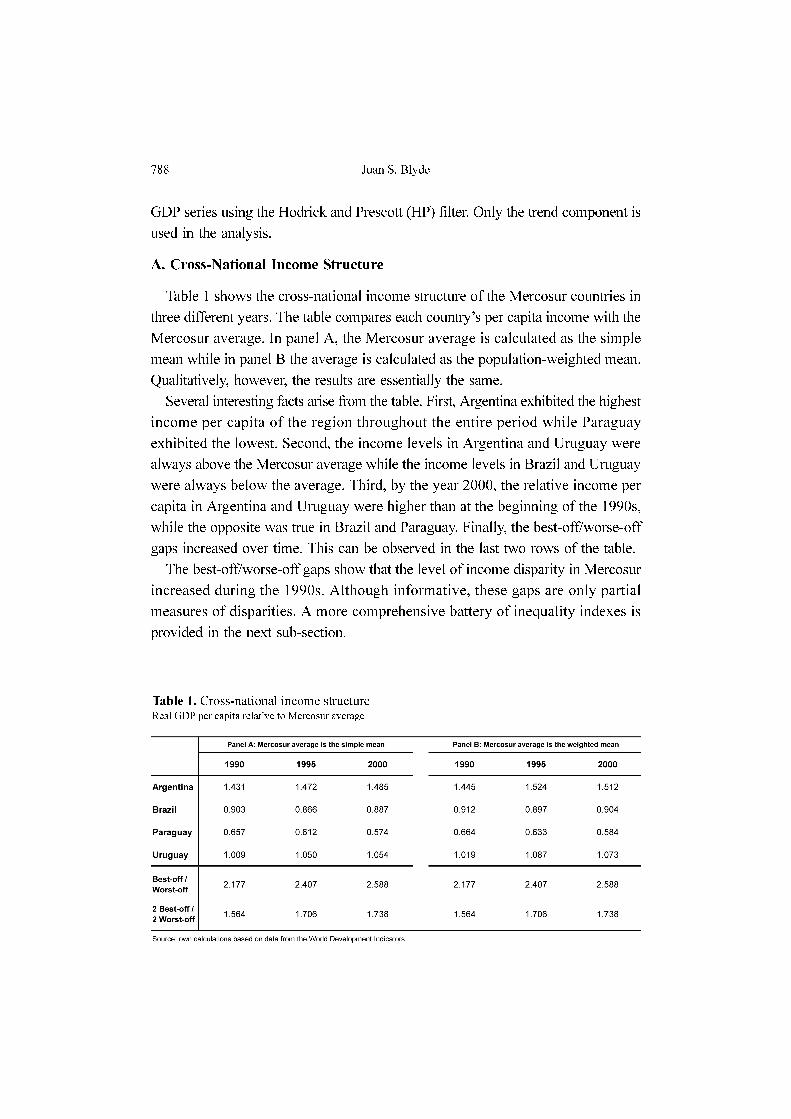
Table 1 shows the cross-national income structure of the Mercosur countries in

three different years. The table compares each country’s per capita income with the

Mercosur average. In panel A, the Mercosur average is calculated as the simple

mean while in panel B the average is calculated as the population-weighted mean.

Qualitatively, however, the results are essentially the same.

Several interesting facts arise from the table. First, Argentina exhibited the highest

income per capita of the region throughout the entire period while Paraguay

exhibited the lowest. Second, the income levels in Argentina and Uruguay were

always above the Mercosur average while the income levels in Brazil and Uruguay

were always below the average. Third, by the year 2000, the relative income per

capita in Argentina and Uruguay were higher than at the beginning of the 1990s,

while the opposite was true in Brazil and Paraguay. Finally, the best-off/worse-off

gaps increased over time. This can be observed in the last two rows of the table.

The best-off/worse-off gaps show that the level of income disparity in Mercosur

increased during the 1990s. Although informative, these gaps are only partial

measures of disparities. A more comprehensive battery of inequality indexes is

provided in the next sub-section.

Table 1. Cross-national income structure

Real GDP per capita relative to Mercosur average


B. Measures of Dispersion Across National Incomes

During the last ten years, there has been a wide used of two convergence concepts

popularized by Barro and Sala-i-Martin (1991, 1992) : the sigma-convergence and

the beta-convergence. They have been employed to analyze the evolution of income

disparities across regions and countries. More recently, however, economists have

started to use, in the same regional and national contexts, some of the inequality

indexes that have been extensively employed in the literature of inequality

measurement with household data, mainly the Gini and Theil indexes (see for

example, Duro and Esteban, 1998; Theil and Moss, 1999; and Duro, 2001).

In this sub-section, we use a battery of three inequality measures to analyze the

income disparity in Mercosur: the sigma-dispersion, the Gini coefficient and the

Theil population-weighted index.3 Given its intrinsically different construction and

interpretation, we analyze the beta-convergence concept in Appendix A.

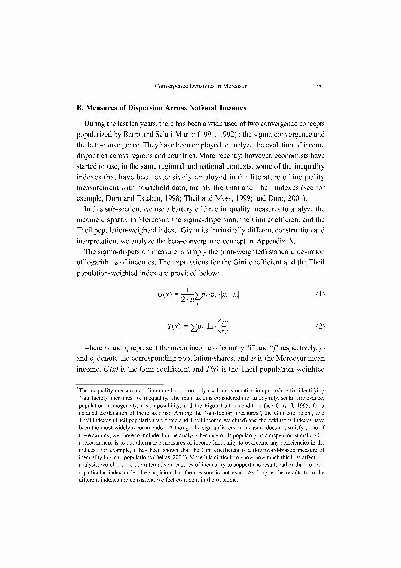
The sigma-dispersion measure is simply the (non-weighted) standard deviation

of logarithms of incomes. The expressions for the Gini coefficient and the Theil

population-weighted index are provided below:

(1)

(2)

where xi and xj represent the mean income of country “i” and “j” respectively, pi

and pj denote the corresponding population-shares, and µ is the Mercosur mean

income. G(x) is the Gini coefficient and T(x) is the Theil population-weighted

G x( ) 1

2 µ⋅---------- pi pj xi xj–⋅ ⋅

i

∑=

T x( ) pi lnµ

xi

---⎝ ⎠⎛ ⎞⋅ ⋅

i

∑=

3The inequality measurement literature has commonly used an axiomatization procedure for identifying

“satisfactory measures” of inequality. The main axioms considered are: anonymity, scalar irrelevance,

population homogeneity, decomposability, and the Pigou-Dalton condition (see Cowell, 1995, for a

detailed explanation of these axioms). Among the “satisfactory measures”, the Gini coefficient, two

Theil indexes (Theil population-weighted and Theil income-weighted) and the Atkinsons indexes have

been the most widely recommended. Although the sigma-dispersion measure does not satisfy some of

these axioms, we chose to include it in the analysis because of its popularity as a dispersion statistic. Our

approach here is to use alternative measures of income inequality to overcome any deficiencies in the

indices. For example, it has been shown that the Gini coefficient is a downward-biased measure of

inequality in small populations (Deltas, 2003). Since it is difficult to know how much this bias affect our

analysis, we choose to use alternative measures of inequality to support the results rather than to drop

a particular index under the suspicion that the measure is not exact. As long as the results from the

different indexes are consistent, we feel confident in the outcome.

790 Juan S. Blyde

index.4

Figure 1 shows the temporal patterns of cross-national inequalities measured by

the three indexes. Similar results arise from all the measures: the income disparity

across the four countries increased throughout most of the 1990s and then

decreases slightly at the end of the decade (except for the sigma-dispersion

measure). Despite the decrease at the end of the 1990s, the evidence from the three

indices clearly shows that income inequality across Mercosur countries increased

through this decade.

Still, a relevant question is: how important are the inequality levels that we observe?

One way to answer this question is to compare the actual values of the selected

measures with their minimum and maximum attainable levels. However, even in

the hypothetical case that the indexes appear to be closer to their lower levels than

to their upper bounds, a low-inequality interpretation might be questionable because

the values could still exceed the maximum level that might be socially and politically

tolerable (Duro, 2001). A second approach, then, is to compare the inequality

values of Mercosur with those from other trade blocs. This exercise might not be

completely satisfactory either because the blocs might be in different stages of

integration processes. With this caveat in mind, however, we compare the national

income disparity in Mercosur with the national income disparity in the European

4The Gini coefficient takes on values between 0 and 1 with zero interpreted as no inequality. The Theil

population-weighted index has a lower bound of zero, which represents perfect equality. Its upper bound

is no homogeneously defined, although values near one can be perceived as an indication of very high

inequality.

Figure 1. Temporal patterns of cross-national inequalities in MERCOSUR


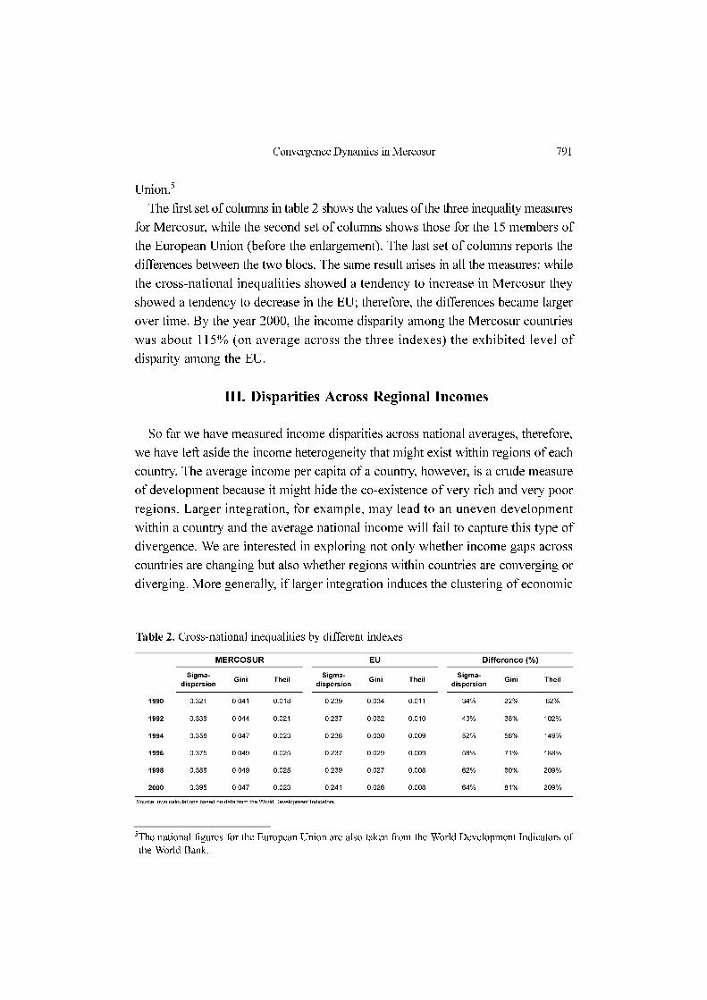
Union.5

The first set of columns in table 2 shows the values of the three inequality measures

for Mercosur, while the second set of columns shows those for the 15 members of

the European Union (before the enlargement). The last set of columns reports the

differences between the two blocs. The same result arises in all the measures: while

the cross-national inequalities showed a tendency to increase in Mercosur they

showed a tendency to decrease in the EU; therefore, the differences became larger

over time. By the year 2000, the income disparity among the Mercosur countries

was about 115% (on average across the three indexes) the exhibited level of

disparity among the EU.

III. Disparities Across Regional Incomes

So far we have measured income disparities across national averages, therefore,

we have left aside the income heterogeneity that might exist within regions of each

country. The average income per capita of a country, however, is a crude measure

of development because it might hide the co-existence of very rich and very poor

regions. Larger integration, for example, may lead to an uneven development

within a country and the average national income will fail to capture this type of

divergence. We are interested in exploring not only whether income gaps across

countries are changing but also whether regions within countries are converging or

diverging. More generally, if larger integration induces the clustering of economic

5The national figures for the European Union are also taken from the World Development Indicators of

the World Bank.

Table 2. Cross-national inequalities by different indexes

792 Juan S. Blyde

activity in a few large cities de-industrializing many other locations, then regions

might be catching up with one another but only within sub-groups. All these

dynamics will be missed by focusing only on income disparities across national

incomes. For this reason, we measure the evolution of income disparities also

across regions. This objective requires us to collect data at the regional level. A

brief summary of the data is provided below.

Data on Argentine’s population by ‘provincias’ is provided by Instituto Nacional de

Estadística y Censos (INDEC) and data on GDP at the same level of aggregation is

provided by the Minister of Interior. Brazil’s data on population and GDP by ‘states’

comes from Instituto Brasileiro de Geografia e Estadística (IBGE). Paraguay’s

population by ‘departamentos’ is taken from the Dirección General de Estadísticas,

Encuestas y Censos (DGEEyC). No official data exists for GDP at this level of

aggregation. Instituto Desarrollo of Paraguay, however, has calculated GDP at this

level of aggregation taking the GDP figures from the national accounts and

imputing them with a geographical distribution based on census data on production,

registries from public institutions, and other factors6. Uruguay’s population figures

by ‘departamentos’ come from Instituto Nacional de Estadística (INE) while data

on GDP at this level of aggregation comes from the Oficina de Planeamiento y

Presupuesto (OPP).

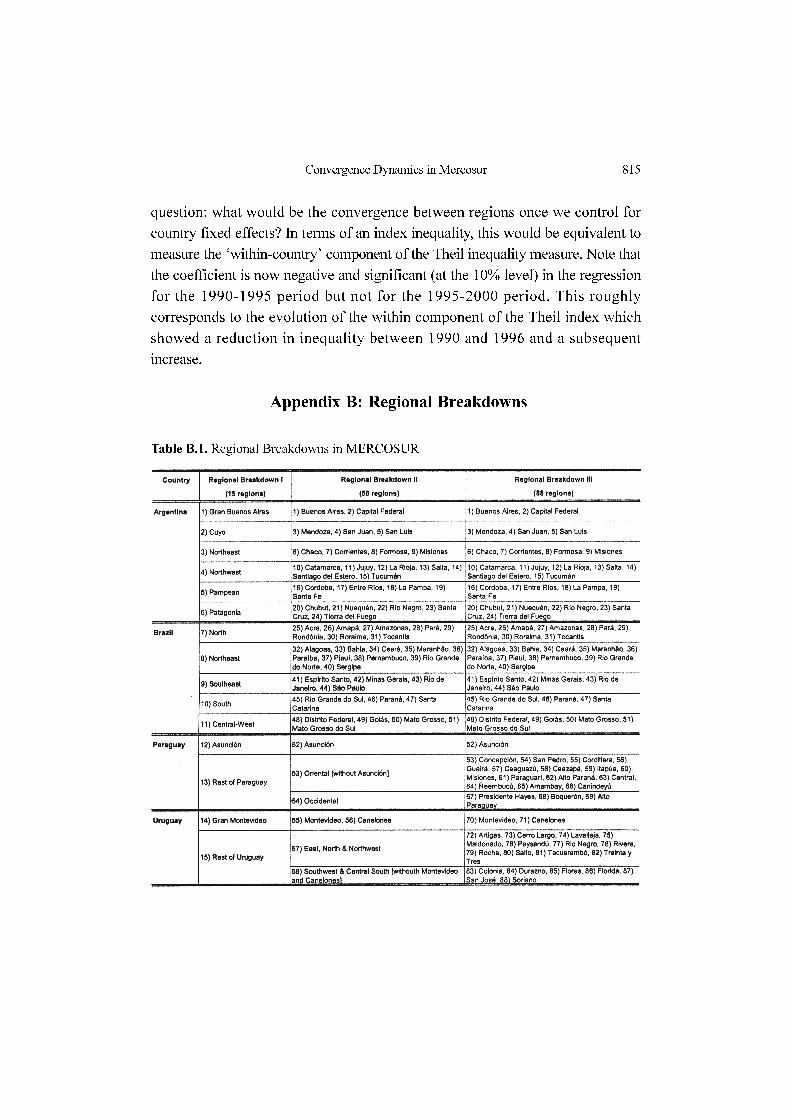
The way the data is divided at the sub-national level in each of the countries

does not necessarily provide appropriate units of comparison. Since any regional

breakdown is going to have some degree of arbitrariness, we decide to deal with

this shortcoming by using not only one regional breakdown but three different

alternatives Our approach here is that by employing different regional breakdowns

we can check how robust the results are. Table B.1 in Appendix B shows the

different regional breakdowns used in the paper.

All the GDP series were transformed into comparable PPP terms at 1995 prices.

Finally, similar to the national data, all the GDP series were filtered with Hodrick

and Prescott to extract their trend components.

A. Measures of Dispersion Across Regional Incomes

We now apply the same battery of inequality indexes to the first regional

breakdown shown in table B.1 (15 regions). Figure 2 shows the results. There is

again a temporal pattern of increasing inequality during the 1990s. This pattern

6For a detailed explanation about this procedure, see Molinas and Buttner, 1999.


emerges with any of the three indexes.

Table 3 shows the actual values of the three indexes for the Mercosur countries

(first set of columns). Note that the values are higher than those reported in table 2

where we only measure inequalities between countries. Therefore, the hetero-

geneity within countries adds to the overall inequality of the Mercosur area. In fact,

we could decompose the overall inequality of Mercosur into two components:

inequality between countries and inequality within countries. We will come back to

this point later. Now, we would like to explore how large is the overall inequality

observed.

Same as before, we compare the inequality levels in Mercosur with the

Figure 2. Temporal patterns of cross-regional Inequalities in Mercosur (15 regions)

Table 3. Cross-regional inequalities by different indexes

794 Juan S. Blyde

inequality levels in the EU. In order to make reasonable comparisons, however, we

first need to construct income inequality measures for the EU at the regional level.

Data at the regional level for the European Union is provided by the REGIO

data bank which is distributed by Eurostat. Different levels of aggregation exists

depending on the regional breakdown NUTS (Nomenclature of Statistics Territorial

Units). In 2002, NUTS 1 divided the entire EU in 77 regions, NUTS 2 in 213

regions and NUTS 3 in 1091 regions7. We choose the first level of aggregation,

NUTS 1, for our comparison.8,9

The second set of columns in table 3 presents the results for the EU, while the

last set of columns reports the differences between the two blocs. Same as before,

the differences increased over time. Note also that the differences that we saw

between the two blocs at the national level are even larger at the regional level. By

2000, the level of regional disparities in Mercosur exceeds in 160% (on average

across the three indexes) the exhibited regional disparities in the EU.

Finally, having shown the results for the highest level of regional aggregation in

table B.1 (15 regions), we now show the results at the other extreme, for the lowest

level of regional aggregation (88 regions). Figure 3 and table 4 present the

findings, which once again confirm the same patterns that we obtained before.10,11

It should be emphasized that the purpose of these comparisons is only

informational. For instance, regional breakdowns are not necessarily equivalent

and, as we mentioned above, the stages of these two integration processes are not

the same. Nevertheless, we feel that the evidence presented so far provides enough

support to argue that the level of income disparity in Mercosur is far from small.

From now on, and to ease the presentation of the paper, we will continue

showing the results only at the third level of aggregation (88 regions). Results

7NUTS 2 is the regionalization used for the distribution of Structural Funds.

8NUTS 1 classification implies an average of 5 regions per country, NUTS 2 an average of 14 regions per

country, and NUTS 3 an average of 73 regions. Therefore, the most reasonable level of aggregation for

the comparison seems to be the NUTS 1 classification.

9With data on GDP and population at the NUTS 1 regional breakdown, we constructed the regional GDP per

capita series. Same as before, the cyclical components of all the GDP series were previously extracted

using the Hodrick-Prescott filter.

10We choose the second level of aggregation, NUTS 2, for the comparison with the EU at this regional

breakdown.

11Using the second level of aggregation (58 regions) also produces similar outcomes.


corresponding to the other two regional breakdowns shall be considered to exhibit

similar patterns unless it is explicitly mentioned otherwise.

B. Inequality Decomposition: Within and Between Groups

A major advantage of the Theil measure is that it can be partitioned into disjoint

subgroups. For a regional analysis, a natural partition would be the use of own

countries. Thus, it is possible to decompose the overall degree of regional

inequality, reflected by T(x), in two different components: the within-country

inequality factor and the between-country inequality factor.12 The first component

is computed as a weighted mean of the intra-country inequality indexes. The

12See, for example, Brulhart and Traeger (2005).

Figure 3. Temporal patterns of cross-regional inequalities in Mercosur (88 regions)

Table 4. Cross-regional inequalities by different indexes

796 Juan S. Blyde

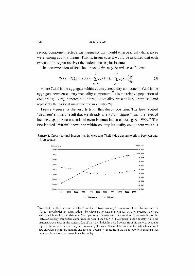
second component reflects the inequality that would emerge if only differences

were among country means. That is, in our case it would be assumed that each

resident of a region receives the national per capita income.

The decomposition of the Theil index, T(x), may be written as follows:

(3)

where TW(x) is the aggregate within-country inequality component; TB(x) is the

aggregate between-country inequality component; is the relative population of

country “g”; T(x)g denotes the internal inequality present in country “g”, and

represents the national mean income in country “g”.

Figure 4 presents the results from this decomposition. The line labeled

‘Between’ shows a result that we already knew from figure 1, that the level of

income disparities across national mean incomes increased during the 1990s.13 The

line labeled “Within” shows the within-country inequality component which is

T x( ) Tw x( ) TB x( ) pg

g 1=

G

∑ T x( )g pg

g 1=

G

∑ lnµ

xg----

⎝ ⎠⎛ ⎞⋅+⋅=+=

gp

13Note that the Theil measure in table 2 and the ‘between-country’ component of the Theil measure in

figure 4 are identical by construction. The values are not exactly the same, however, because they were

calculated from different data sets. More precisely, the national GDPs used in the construction of the

between-country component come from the sum of the GDPs of the regions in each country while the

national GDPs used in the construction of the Theil index in table 2 comes from the national accounts

figures. As we noted above, they are not exactly the same. Some of the series at the sub-national level

are calculated from estimations and do not necessarily come from the same public institutions that

produce the national accounts in each country.

Figure 4. Cross-regional inequalities in Mercosur Theil index decomposition: between and

within groups


basically a weighted average of the level of regional inequality that is present in

each of the countries. Interestingly, this component shows a slight U-trend. This is,

it decreases slightly until 1996 and then starts to increase. Does this mean that

regional inequality in each of the countries showed the same trend? Not

necessarily, as the index only reflects an average of the four countries. In fact, this

trend can be caused by several different situations, so we need to explore the

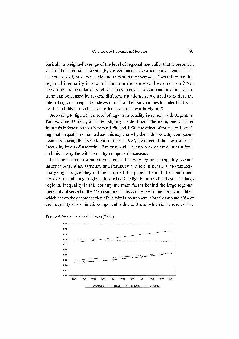
internal regional inequality indexes in each of the four countries to understand what

lies behind this U-trend. The four indexes are shown in Figure 5.

According to figure 5, the level of regional inequality increased inside Argentina,

Paraguay and Uruguay and it felt slightly inside Brazil. Therefore, one can infer

from this information that between 1990 and 1996, the effect of the fall in Brazil’s

regional inequality dominated and this explains why the within-country component

decreased during this period, but starting in 1997, the effect of the increase in the

inequality levels of Argentina, Paraguay and Uruguay became the dominant force

and this is why the within-country component increased.

Of course, this information does not tell us why regional inequality became

larger in Argentina, Uruguay and Paraguay and felt in Brazil. Unfortunately,

analyzing this goes beyond the scope of this paper. It should be mentioned,

however, that although regional inequality felt slightly in Brazil, it is still the large

regional inequality in this country the main factor behind the large regional

inequality observed in the Mercosur area. This can be seen more clearly in table 5

which shows the decomposition of the within-component. Note that around 80% of

the inequality shown in this component is due to Brazil, which is the result of the

Figure 5. Internal national indexes (Theil)

798 Juan S. Blyde

high regional inequality of the country together with the fact that Brazil is the largest

country of the four, and thus has the largest population weight in the within component.

Before moving to the next section, it might be instructive to apply the above

inequality decomposition to the EU area. After all, the EU has been using policy

instruments to promote convergence at the regional level, and so, it would be

interesting to analyze whether there have been signs of regional convergence inside

EU countries. Figure 6 shows the results.

Table 5. Decomposition of inequality (within) among countries

Figure 6. Cross-regional inequalities in the EU

Theil index decomposition: between and within groups


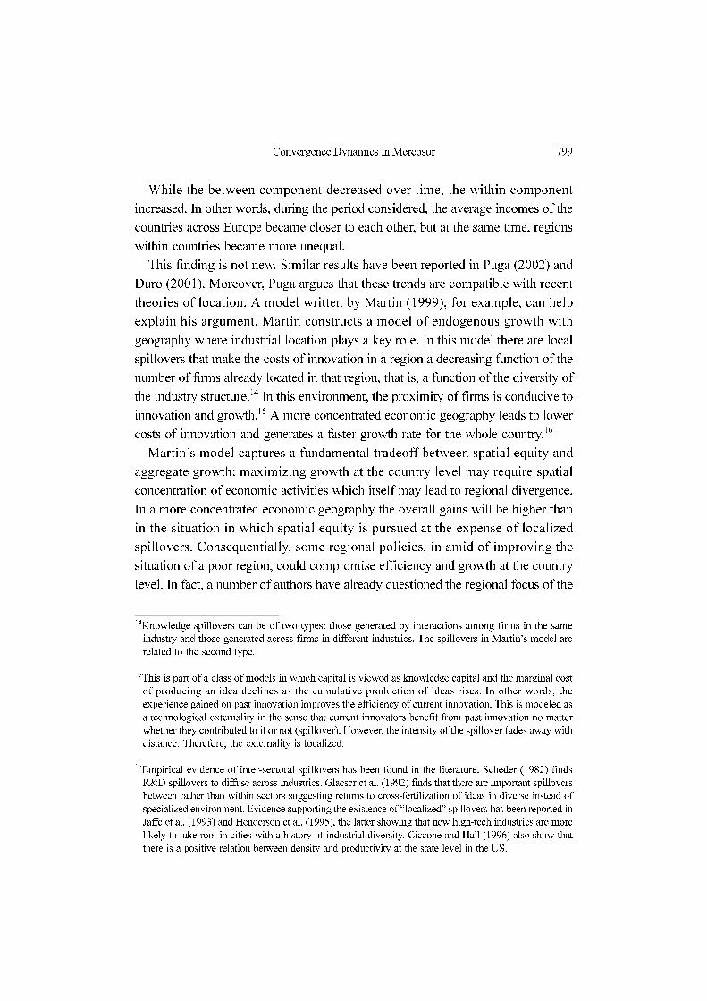
While the between component decreased over time, the within component

increased. In other words, during the period considered, the average incomes of the

countries across Europe became closer to each other, but at the same time, regions

within countries became more unequal.

This finding is not new. Similar results have been reported in Puga (2002) and

Duro (2001). Moreover, Puga argues that these trends are compatible with recent

theories of location. A model written by Martin (1999), for example, can help

explain his argument. Martin constructs a model of endogenous growth with

geography where industrial location plays a key role. In this model there are local

spillovers that make the costs of innovation in a region a decreasing function of the

number of firms already located in that region, that is, a function of the diversity of

the industry structure.14 In this environment, the proximity of firms is conducive to

innovation and growth.15 A more concentrated economic geography leads to lower

costs of innovation and generates a faster growth rate for the whole country.16

Martin’s model captures a fundamental tradeoff between spatial equity and

aggregate growth: maximizing growth at the country level may require spatial

concentration of economic activities which itself may lead to regional divergence.

In a more concentrated economic geography the overall gains will be higher than

in the situation in which spatial equity is pursued at the expense of localized

spillovers. Consequentially, some regional policies, in amid of improving the

situation of a poor region, could compromise efficiency and growth at the country

level. In fact, a number of authors have already questioned the regional focus of the

14Knowledge spillovers can be of two types: those generated by interactions among firms in the same

industry and those generated across firms in different industries. The spillovers in Martin’s model are

related to the second type.

15This is part of a class of models in which capital is viewed as knowledge capital and the marginal cost

of producing an idea declines as the cumulative production of ideas rises. In other words, the

experience gained on past innovation improves the efficiency of current innovation. This is modeled as

a technological externality in the sense that current innovators benefit from past innovation no matter

whether they contributed to it or not (spillover). However, the intensity of the spillover fades away with

distance. Therefore, the externality is localized.

16Empirical evidence of inter-sectoral spillovers has been found in the literature. Scheder (1982) finds

R&D spillovers to diffuse across industries. Glaeser et al. (1992) finds that there are important spillovers

between rather than within sectors suggesting returns to cross-fertilization of ideas in diverse instead of

specialized environment. Evidence supporting the existence of “localized” spillovers has been reported in

Jaffe et al. (1993) and Henderson et al. (1995), the latter showing that new high-tech industries are more

likely to take root in cities with a history of industrial diversity. Ciccone and Hall (1996) also show that

there is a positive relation between density and productivity at the state level in the US.

800 Juan S. Blyde

EU convergence policy on similar grounds.17 Not surprisingly, a recent indepen-

dent report commissioned by the EU calls for a change in the convergence policy

to focus on countries, rather than regions, using national GDP per capita as an

eligibility criterion (see Sapir, 2003).

As we already mentioned in other parts of this paper, care should be exercised

when comparing two integrating blocs because of their potentially different

development stages, but the above results deserve a reflection. The EU has only

exhibited convergence across national incomes. If convergence across regions

within countries has not been achieved given all the resources dedicated to this end,

one might wonder how this goal could be achieved in Mercosur with considerably less

financial resources potentially available. We will come back to this point later.

IV. Inequality Changes: Income & Population Changes

The analysis in the previous section has shown an increasing trend of regional

inequality in Mercosur. In this section we analyze the role of income and

population changes in shaping this trend.

Intertemporal changes in regional inequalities are normally perceived in terms of

variations in per capita incomes. For example, an upward inequality tendency like

the one that we see in Mercosur is conventionally viewed as an indication of a

widening in regional income distances. This interpretation might be misleading,

however. Variations in the population shares can also play a significant role in the

inequality changes.

The following example, provided by Duro (2001), illustrates this point. Suppose

one wants to measure the inequality between two regions, a poorer and a richer

one. The richer region has two times the income of the poorer region, but the

poorer region has a population share of 80%. We can assume that people move

from the poorer region to the richer one, finding a better quality of life to such a

point that in the end all the population is concentrated in the rich region. We also

assume that no changes occur in regional mean incomes. In these circumstances,

regional inequality will display an initial growth until a point after which a declining

pattern will be observed.18 Thus, intertemporal inequality changes might be due

exclusively to demographic movements.

17See for example, Martin (1998, 1999), Midelfart-Knarvik and Overman (2002), and Puga (2002).

18This argument was first raised by Robinson (1976).


It would be important to understand the role played by each factor in Mercosur

because implications can be very different. For example, a situation in which

regional mean incomes remain roughly the same but population changes are

temporarily driving the inequality measure up (as in the example above) might call

for different policy actions than a situation in which regional mean incomes are

diverging. A focus on migration policies might be a reasonable prescription in the

first case while targeting the roots of regional growth differentials might be the

relevant aspect in the latter.

One way to explore the relevance of income and population changes can be

done using the following expression:

(4)

where I denotes an income inequality index, xT and xT+1, are the per capita

incomes vectors in periods T and T+1, respectively; and pT and pT+1, are the

population-shares at T and T+1, respectively.

The first term in the right-hand side of equation (4) captures the influence of

income changes, while the second term captures the influence of population

changes over regions, leaving regional incomes constant over time.

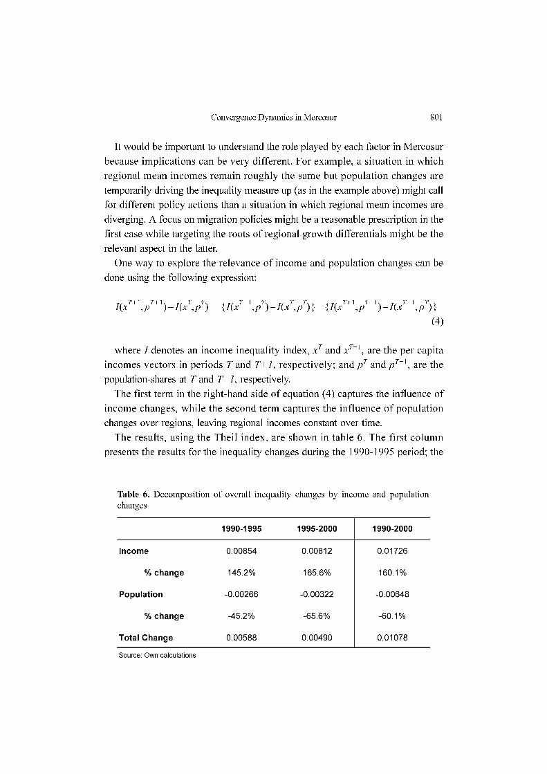
The results, using the Theil index, are shown in table 6. The first column

presents the results for the inequality changes during the 1990-1995 period; the

I xT 1+

pT 1+

,( ) I xT

pT

,( )– I xT 1+

pT

,( ) I xT

pT

,( )–{ } I xT 1+

pT 1+

,( ) I xT 1+

pT

,( )–{ }+=

Table 6. Decomposition of overall inequality changes by income and population

changes

802 Juan S. Blyde

second column presents the results for the inequality changes during the period

1995-2000, and the last column does the same for the entire 1990-2000 period. In

all the cases, the income and the population changes move in opposite directions

with income changes moving the inequality measure upwards and the population

changes moving the inequality measure downwards. Therefore, changes in the

distribution of people across regions reduced the inequality levels in Mercosur;

however, the average income across regions became more unequal and more than

compensated the demographics effect. Thus, the overall inequality level increased.

The findings in table 6 underline two relevant aspects: first, demographics is not

a static factor. The results seem to suggest that migration has played some role in

ameliorating the standards of living of those moving away from regions that have

not been able to offer enough opportunities. Second, in order to understand why

regional inequality increased in Mercosur, one need to understand why some

regions have experienced higher income growth than others. This is the root of the

increase in the inequality observed in the Mercosur area. The next section sheds

light on this important issue.

V. Distribution Dynamics

So far, we have used inequality indexes to explore the evolution of income

disparities across Mercosur regions. These indexes indicate that there has been an

increase in inequality across Mercosur regions during the 1990s. Section 4

specifically shows that this is not a result of population changes. If anything,

demographics movements have played an ameliorating role.

The above findings suggest that the distribution of regional mean incomes might

have become more polarized. This is, the gap between the rich and the poor

regions has become wider. Unfortunately, one limitation of employing indexes is

that they provide little information on what happen inside the income distribution.

For instance, we might want to know whether there have been persistence in some

parts of the distribution, or whether there have been the formation of clubs. Did the

rich regions converge to each other leaving the poor regions to form a different

convergence club? These questions cannot be analyzed with the traditional indexes

of inequality because they do not convey any information on how the relative

positions of the regions changed over time. In this section we take care of this

shortcoming by using a distribution dynamics approach. This approach has been

employed by a number of authors, including Quah (1996a).


The distribution dynamics approach moves away from characterizing convergence

by using single indexes or regression analyses. It involves tracking the evolution of

the entire income distribution itself over time. Markov chains are employed to

approximate and estimate the laws of motion of the evolving distribution. The

intra-distribution dynamics information is normally encoded in a transition

probability matrix. This approach has revealed empirical regularities such as

convergence clubs, polarization, or stratification of countries or regions catching up

with one another but only within sub-groups.19

We begin our analysis by constructing a 5x5 Markov transition probability

matrix.20 The transition probability matrix in table 7 shows transitions between the

1990 and 2000 distributions of GDP per capita relative to the Mercosur mean.21

The 45 degree diagonal shows the proportion of regions that remain in the same

range of the distribution between the two years. The last row, for example, shows

that from the 16 regions that exhibited a GDP per capita below 0.51 times the

19See Quah (1996b) for the underlying formal structure of these models.

20This entire section was done using Quah’s TSRF econometrics shell.

21The income states of the transitional probability matrix are selected so that the observed data in the base

year is divided into roughly equal-sized categories. This is the standard practice.

Table 7. Transition probability matrix

804 Juan S. Blyde

Mercosur average during 1990, 94% remained in the same range in 2000, while

6% experienced an increase in their relative income to between 0.51 and 0.64 times

the Mercosur average. None of the regions moved higher up in the distribution.

The large numbers in the diagonal show the persistence of relative regional

income, specially at the lower and upper ends. Note that the regions in the middle

of the distribution have a larger propensity to move. Interestingly, if the region had

an income per capita between 0.51 and 0.83 times the Mercosur average, the

region experienced a higher tendency to move to the lower part of the distribution

than to the upper part. On the other hand, if the region had an income per capita

above 0.83 times the Mercosur average, the region experienced a higher tendency

to move to the upper part of the distribution than to the lower part. As a consequence,

the distribution became more dense in the tails, specially in the lower tail, and

thinned out in the middle. In other words, in 2000 there were fewer regions in the

middle of the distribution as compared to 1990 and more regions closer to the tails,

specially the lower tail.

We can further assume that the system described by the transition probability

matrix continues in its evolution. In other words, the transition that took place

between 1990 and 2000 occurs again several times. If nothing structural were to

change, then the system could eventually reach a long-run steady state. This is

what is called the ergodic distribution (or the steady state distribution), and it is

shown in the last row of the table. This is obtained by iterating the transition

probability matrix repeatedly over the long horizon to get an estimation of the long

run tendency of a region to land up in a given income range. The results indicate a

tendency towards a two-point asymmetrical distribution suggesting the formation

of two unbalanced clubs: a very large club at the bottom of the distribution, and a

very small club at the top part.22

One shortcoming of the transition probability matrix is that the selection of

income states is arbitrary -different sets of discretisations may lead to different

results. For instance, the ergodic distribution may change under different income

states.23 One way to overcome this drawback is by using the stochastic kernel.

22It should be mentioned that the ergodic distribution shall not be read as a forecast of the future.

Government policies might change, important events might occur, and many forces behind the

widening of income gaps might exhibit non-linear effects. Therefore, the ergodic distribution shall be

interpreted simply as the long run realization of similar tendencies in the absence of structural changes

(Quah, 1996a).

23Bulli (2001) shows how discretisations could affect the results by removing the Markov property.


The stochastic kernel replaces the discrete income states of the transition

probability matrix by a continuum of states. This means that we no longer have a

grid of fixed income states, like [0.0-0.51), [0.51-0.64) , etc, but allow the states to

be all possible intervals of income. By this we remove the arbitrariness in the

discretisation of the states. We now have an infinite number of rows and columns

replacing the transition probability matrix. The stochastic kernel can be viewed as a

continuous version of the transition probability matrix. Figure 7 shows the

stochastic kernel for relative per capita income of 10-year transitions between 1990

and 2000. Figure 8 shows the corresponding contour plot.

Interpretation of the stochastic kernel is as follows. Stand at any point on the

Period t axis, and then look in a straight line parallel to the Period t+10 axis. What

is traced out on the surface of the kernel is a probability density: it is always non-

negative and integrates to 1. The more likely transition possibilities manifest as

higher values on this line. The 45-degree diagonal indicates persistence properties:

regions in different parts of the income distribution remain roughly where they

begin. The more pronounced the surface along this diagonal, the more persistence

there is in the distribution. The lower is this diagonal, the greater is the intra-

distribution mixing. A single ridge parallel to the Period t axis indicates

Figure 7. Stochastic Kernel, 3d plot Dynamics of cross-regional distribution of income per

capita 10-year transitions

806 Juan S. Blyde

convergence: poor regions growing faster and rich regions slowing down so

eventually all income levels are equalized. Another extreme occurs when piling up

takes place along the negative-sloped diagonal which shows regions dynamically

overtaking one another. Peaks indicate club behavior: regions around a particular

income class become attached, over time, to precisely such income class (this is a

peak that is on the 45-degree diagonal) or to a different income class (this is a peak

that is off the 45-degree diagonal).

Observation of the stochastic kernel in figure 7 shows a ridge that lays close to

the 45-degree diagonal. For certain income ranges, the ridge is slightly off the

diagonal. For example, for very low income levels the ridge is situated slightly

below the diagonal and for mid income levels the ridge lays slightly above the

diagonal. This can be verified in the contour plot of the stochastic kernel which is

shown in figure 8. For regions with incomes around 0.5 times the Mercosur

average (and below), the highest probability occurs somewhat at higher incomes,

so these regions had a higher tendency to move slightly up in the distribution than

to a lower part. For income levels between 0.6 and 1.8 times the Mercosur average

the opposite was true. Regions that started within this income range had a higher

tendency to move slightly lower in the distribution than to the upper part. Note that

Figure 8. Stochastic Kernel, contour plot Dynamics of cross-regional distribution of income

per capita 10-year transition


this tendency to move lower in the distribution decreases for incomes above 1.8

times the Mercosur average and eventually disappears.

Figures 7 and 8 also show that the ridge drops dramatically for incomes

immediately above 1.8 times the Mercosur average. This implies that persistence

was very low in this area. Then, at incomes around 2.2 times the Mercosur

average, the ridge increases again implying a rise in persistence.

From the above results, we can say that the most relevant features of the

distribution dynamics between 1990 and 2000 were the following: (i) for regions at

the bottom part of the distribution, the main tendency was to move slightly higher

up in the distribution; (ii) for regions at the low-middle and middle part, the main

tendency was to move lower; (iii) for those at the middle-high part of the

distribution, the main feature was the low persistence observed (although no

particular propensity to move higher or lower in the distribution was identified);

and (iv) for those at the very top of the distribution, the main characteristic was the

existence of some persistence.

These findings suggest a bias towards the accumulation of regions in the low-

middle part of the distribution primarily due to the relative impoverish of regions

with mid incomes. Since the regions at the very top appears to exhibit some

persistence, the results from the stochastic kernel suggest a tendency towards a two

club formation. Note, however, that the upper peak is imprecisely estimated. The

reason for this is that in this area there are relatively fewer observations.24

Nevertheless, the results seemingly confirm the outcome from the ergodic distribu-

tion of a tendency towards a two-asymmetrical club formation: a very large club

consisting of low and low-mid income regions and a small club of rich regions. Is

this trend the result of larger integration in Mercosur?, could it be associated with

the agglomeration forces unleashed by lower trade barriers?. Answers to these

questions belong to a much wider research agenda, however, before concluding,

we provide some evidence about the role of these forces in Mercosur.

As stated in the introduction, the existence of scale economies or the presence of

local spillovers may create tendencies for the agglomeration of industrial activity.

Therefore, factor mobility and opening to trade may exaggerate initial differences

in size and income. According to Venables (1999), agglomeration forces in industrial

24The places in the stochastic kernel where more grid lines are drawn are the places where more

observations are available and so the resolution is correspondingly finer. The places where the surface

is mostly white space are the places where there are relatively fewer observations and the precision of

the estimate is lower.

808 Juan S. Blyde

countries can act at a quite narrow sectoral level creating clusters of different

industries across different regions, in which case it might not lead to divergence of

per capita income levels. However, agglomeration forces among low income

countries may instead follow a pattern in which manufacturing as a whole comes

to cluster in a few locations de-industrializing the less favored regions. There are at

least two reasons for this. First, manufacturing does not normally represent a large

share of the economy in low income countries, so fitting it in a few locations will

not lead to a rise in the price of the immobile factors, such as land. Second, at early

stages of development, the basic industrial infrastructure that support production

(such as transport, telecommunications, access to financial markets and other

business centers) is typically underdeveloped and available only in few locations.

Agglomeration forces will push industrial activities to concentrate in those locations.

What is the evidence regarding this effect?. Sanguinetti, et al. (2004) estimate a

model in which the patterns of industrial location in Mercosur are explained by

several factors including relative endowments, market potential and industrial

linkages. The study shows that sectors that exhibit increasing returns to scale and

sectors that use intensively intermediate inputs indeed tend to locate in the

countries that exhibit large market potential. However, the authors find that since

the creation of Mercosur this tendency has declined. They take this as an indication

that the agglomeration forces have somewhat debilitated with the implementation

of the agreement.

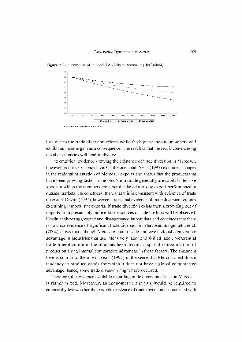
Another piece of evidence consists on measures of concentration of industrial

activity in Mercosur. This is shown in figure 9. The concentration measure is a

Herfindalh index which is constructed as the sum of the squares of the share of

Mercosur’s total manufacturing activity in region i. The figure shows concentration

measures at the country level and also at two regional levels of aggregation taken

from Appendix B: regional breakdown I (15 regions) and regional breakdown III

(88 regions). In all the cases, the result is the same: the concentration of industrial

activity in Mercosur has declined, not increased, during the 1990s. Therefore, it is

difficult to argue that the raise in income disparities that we observed during the

last decade is associated with the concentration of industrial activity in Mercosur.

As stated in the introduction, another alternative is related to the well-known

effect of trade diversion in RIAs. A country experiences trade diversion when

imports from partner countries displace lower cost imports from the rest of the

world. Venables (2003) argues that RIAs among a group of low income countries

might generate a tendency for the lowest income members to suffer a real income


loss due to the trade diversion effects while the highest income members will

exhibit an income gain as a consequence. The result is that the real income among

member countries will tend to diverge.

The empirical evidence showing the existence of trade diversion in Mercosur,

however, is not very conclusive. On the one hand, Yeats (1997) examines changes

in the regional orientation of Mercosur exports and shows that the products that

have been growing faster in the bloc’s intratrade generally are capital intensive

goods in which the members have not displayed a strong export performance in

outside markets. He concludes, then, that this is consistent with evidence of trade

diversion. Devlin (1997), however, argues that evidence of trade diversion requires

examining imports, not exports. If trade diversion exists then a crowding out of

imports from presumably more efficient sources outside the bloc will be observed.

Devlin analyzes aggregated and disaggregated import data and concludes that there

is no clear evidence of significant trade diversion in Mercosur. Sanguinetti, et al.

(2004) shows that although Mercosur countries do not have a global comparative

advantage in industries that use intensively labor and skilled labor, preferential

trade liberalization in the bloc has been driving a spatial reorganization of

production along internal comparative advantage in these factors. The argument

here is similar to the one in Yeats (1997) in the sense that Mercosur exhibits a

tendency to produce goods for which it does not have a global comparative

advantage, hence, some trade diversion might have occurred.

Therefore, the evidence available regarding trade diversion effects in Mercosur

is rather mixed. Moreover, an econometric analysis would be required to

empirically test whether the possible existence of trade diversion is associated with

Figure 9. Concentration of Industrial Activity in Mercosur (Herfindahl)

810 Juan S. Blyde

the income divergence observed.

Finally, there is a possibility that factors other than the creation of Mercosur

have been at the origin of the increased in income disparities. Using tables 3 and 4

it is easy to confirm that the increase in regional disparities that Mercosur

experienced during the 1990s represents only around 10% of the disparities that

already existed in the bloc at the beginning of this decade. Therefore, one could not

rule out the possibility that the income divergence that took place during the 1990s

was just the continuation of previous trends.

VI. Concluding Remarks

This paper uses inequality indexes and a distribution dynamics approach to

measure the evolution of income disparities across countries and regions in

Mercosur. According to the traditional trade theory, a gradual opening of trade

teamed with migration would make initially asymmetric regions more symmetric.

In stark contrast, the new economic geography models show that factor mobility

and opening may eventually exaggerates initial differences. Therefore, the mere

possibility that larger integration could be the origin of income divergence renders

important to analyze the evolution of income disparities in Mercosur.

The techniques used in this paper reveal several interesting points. First, the

level of income disparities across countries and regions in Mercosur increased

during the 1990s. Second, the income inequality observed is very high relative to

the international experience, particularly the EU. Third, although income disparities

increased, results indicate that migration might have played a role in reducing

regional inequality through the movement of people away from regions that have

been able to offer enough opportunities. Fourth, behind the increase in income

disparities across Mercosur regions there seems to be a tendency for a two asymmetrical

club formation: a small club of rich regions and a large club of low and low-mid

income regions that have become larger over time by the relative impoverish of

regions in the middle of the distribution. Fifth, the agglomeration of industrial

activity - typically regarded as one of the main causes of income divergence in

South-South RIAs - has been declining not increasing in Mercosur. Combined with

this, it is worth noting that the increase in income disparities during the 1990s

represents only around 10% of the disparities that already existed in the bloc at the

beginning of this decade. Therefore, one could not rule out the possibility that the

divergence observed during the last decade was a continuation of previous trends


rather than the result of the Mercosur agreement.

A word of caution is in order here. Even if one argues that Mercosur might have

not been at the origin of increasing inequalities in the bloc, the potential for the

agreement to generate income divergence in the future should not be

underestimated. Internal tariffs have been practically removed in Mercosur but

several non-tariff-barriers (NTBs) still remain and trade within the bloc has been

affected by several macroeconomic and financial crises including important

exchange rate re-alignments with severe disrupting effects. Moreover, even though

labor moves freely across regions within countries, migration across national

borders is still limited. Therefore, a deeper integration scenario with larger move-

ment of goods and factors within the bloc could bring some of the forces that

create divergence right into the front stage.

Finally, the analysis of the EU experience brings some interesting points of

comparison. Several studies, including this paper, show that in Europe, income

disparities among EU countries have been declining but income disparities across

regions within countries have been increasing. This latter trend has been observed

in spite of the EU convergence policy and has been considered to be compatible

with recent theories of location. This raises a point of consideration for Mercosur:

regional income disparities in Mercosur are much larger than in the EU and the

amount of potentially available resources to deal with cohesion objectives are

much lower. Therefore, the extent to which regional income disparities in

Mercosur can be effectively reduced with policy intervention should be carefully

analyzed in order to establish realistic goals.

Acknowledgments

This paper has been benefited from conversations with Eduardo Fernández-

Arias and Mauricio Moreira Mesquita. I thank Christian Volpe, Pablo Sanguinetti,

José G. Pineda, Christian Daude and participants in the LACEA meetings in Paris

2005 for helpful comments and suggestions. The views expressed in this paper are

my responsibility and are not necessarily shared by the Inter-American

Development Bank.

Received 1 February 2006, Accepted 12 September 2006

812 Juan S. Blyde

References

Barro, R. and X. Sala-i-Martin (1991) “Convergence across states and regions”, Brookings

Papers on Economic Activity, 1.

Barro, R. and X. Sala-i-Martin (1992) “Convergence”, Journal of Political Economy, 100.

Brulhart, M. and R. Traeger (2005) “An Account of Geographic Concentration Patterns in

Europe”, Regional Science and Urban Economics, 35.

Bulli, S. (2001) “Distribution Dynamics and Cross-Country Convergence : A New

Approach”, Scottish Journal of Political Economy, 48.

Ciccone, A. and R. Hall (1996) “Productivity and the density of economic activity”

American Economic Review, 67.

Cowell, F. (1995), Measuring Inequality, Harvester Wheatsheaf, London

Deltas, G. (2003), “The Small-Sample Bias of the Gini Coefficient: Results and

Implications for Empirical Research”, The Review of Economics and Statistics, 85.

Devlin, R. (1997), “In Defense of Mercosur”, Revista Brasileira de Comercio Exterior,

12.

Duro, J.A. and J. Esteban (1998) “Factor decomposition of cross-country income

inequality”, Economic Letters, 60.

Duro, J.A. (2001) “Regional income inequalities in Europe: an updated measurement and

some decomposition results”. Processed, Instituto de Análisis Económico CSIC.

Glaeser, E.L., H. Kallal, J. Scheinkman, and A. Schleifer (1992) “Growth in cities”

Journal of Political Economy, 100.

Henderson, V., A. Kuncoro, and M. Turner (1995) “Industrial development in cities”

Journal of Political Economy, 103.

Jaffe, A., and M. Trajtenberg (1993) “Geographic localization of knowledge spillovers as

evidenced by patent citations” Quarterly Journal of Economics, 108.

Krugman, P. (1991) “Increasing returns and economic geography” Journal of Political

Economy, 99.

Martin, P. (1998) “Can regional policies affect growth and geography in Europe?”, World

Economy, 21.

Martin, P. (1999) “Public policies, regional inequalities and growth” Journal of Public

Economics, 73.

Midelfart-Knarvik, K.H. and H.G. Overman (2002) “Delocation and European

integration: is structural spending justified?”, Economic Policy, 17.

Molinas, J. and J.E. Buttner (1999) “Estimaciones del PIB municipal en Paraguay”,

mimeo.

Puga, D. (2002) “European regional policies in light of recent location theories”, Journal

of Economic Geography, 2.

Robinson, S. (1976) “A note on the U-hypothesis relating income inequality and

economic development”, American Economic Review, 66.

Sanguinetti, P., I. Traistaru and C. Volpe (2004) “The Impact of South-South Preferential


Trade Agreements on Industrial Development: An Empirical Test”, mimeo.

Sapir, A. (2003) “An agenda for a growing Europe. Making the EU economic system

deliver” Report of an independent high-level study group established on the initiative

of the President of the European Commission.

Slaughter, M. (1997) “Per capita income convergence and the role of international trade”

American Economic Review, 87.

Scheder, F. (1982) “Inter-industry technology flows and productivity growth” Review of

Economics and Statistics, 64.

Theil, H. and C. Moss (1999 ) “The measurement of inequality by components of total

expenditure” Empirical Economics, 24.

Quah, D.T. (1996a) “Convergence empirics across economies with (some) capital

mobility”, Journal of Economic Growth, 1.

(1996b) “Twin peaks: growth and convergence in models of distribution dynamics”

Economic Journal, 106.

Venables, A. (1999) “Regional integration agreements: a force for convergence or

divergence?”, World Bank document.

Venables, A. (2003) “Winners and losers from regional integration agreements” Economic

Journal, 113.

Viner, J. (1950), The Customs Union Issue, New York.

Yeats, A. (1997), “Does Mercosur’s trade performance raise concerns about the effects of

regional trade arrangements?”, World Bank Policy Research Working Paper, 1729.

Appendix A: Measuring Beta Unconditional Convergence

As we mentioned above, the sigma and beta convergence concepts have been

widely employed to analyze income disparities across regions and countries. The

two concepts are intimately related. While sigma convergence refers to a decline in

the dispersion of incomes across regions (measured, for example, by the standard

deviation of the logarithm of per capita incomes), the beta convergence refers to

the situation in which a poor region tends to grow faster than a rich one, so that the

first one tends to catch up with the latter in terms of the level of income per capita.

Barro and Sala-i-Martin (1991) show that both concepts of convergence are

related. In fact, beta convergence is a necessary but not sufficient condition for

sigma convergence because the latter process can be offset by new disturbances

that tend to increase dispersion. We start with the concept of beta unconditional

convergence.

Since we already observed that sigma convergence did not occur in the Mercosur

countries, we can expect that beta convergence would not occur either. However,

for the sake of completeness, we show the results for the beta convergence in

814 Juan S. Blyde

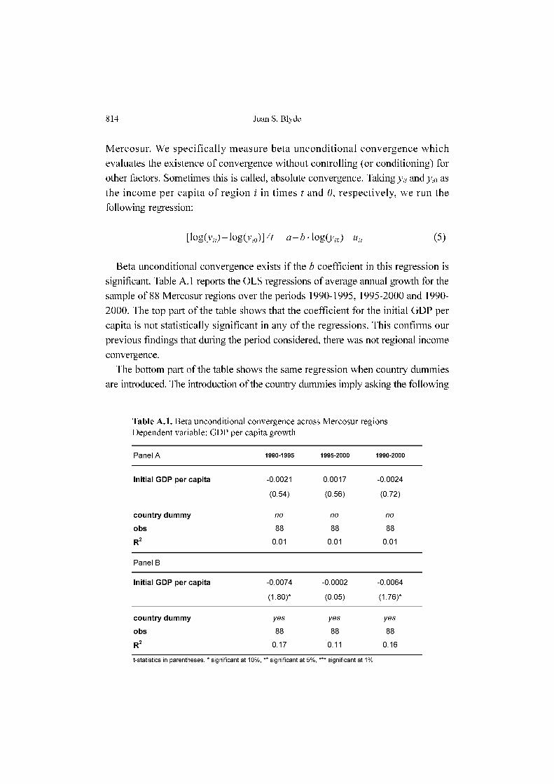
Mercosur. We specifically measure beta unconditional convergence which

evaluates the existence of convergence without controlling (or conditioning) for

other factors. Sometimes this is called, absolute convergence. Taking yit and yi0 as

the income per capita of region i in times t and 0, respectively, we run the

following regression:

(5)

Beta unconditional convergence exists if the b coefficient in this regression is

significant. Table A.1 reports the OLS regressions of average annual growth for the

sample of 88 Mercosur regions over the periods 1990-1995, 1995-2000 and 1990-

2000. The top part of the table shows that the coefficient for the initial GDP per

capita is not statistically significant in any of the regressions. This confirms our

previous findings that during the period considered, there was not regional income

convergence.

The bottom part of the table shows the same regression when country dummies

are introduced. The introduction of the country dummies imply asking the following

log yit

( ) log yi0( )–[ ] t⁄ a b log y

i0( ) uit

+⋅–=

Table A.1. Beta unconditional convergence across Mercosur regions

Dependent variable: GDP per capita growth


question: what would be the convergence between regions once we control for

country fixed effects? In terms of an index inequality, this would be equivalent to

measure the ‘within-country’ component of the Theil inequality measure. Note that

the coefficient is now negative and significant (at the 10% level) in the regression

for the 1990-1995 period but not for the 1995-2000 period. This roughly

corresponds to the evolution of the within component of the Theil index which

showed a reduction in inequality between 1990 and 1996 and a subsequent

increase.

Appendix B: Regional Breakdowns

Table B.1. Regional Breakdowns in MERCOSUR

Convergence Dynamics in Mercosur - Journal of … · Convergence Dynamics in Mercosur ... According...

Documents

Transcript of Convergence Dynamics in Mercosur - Journal of … · Convergence Dynamics in Mercosur ... According...