Convergence analysis of Crankâ€“Nicolson and Rannacher time

Convergence analysis of Crank–Nicolson andRannacher time-marching

Michael B. GilesOxford University Computing Laboratory, Wolfson Building, Parks Road, Oxford OX1 3QD, UK

Rebecca CarterOxford University Computing Laboratory, Wolfson Building, Parks Road, Oxford OX1 3QD, UK

This paper presents a convergence analysis of Crank–Nicolson and Rannachertime-marching methods which are often used in finite difference discretizationsof the Black–Scholes equations. Particular attention is paid to the importantrole of Rannacher’s startup procedure, in which one or more initial timestepsuse backward Euler timestepping, to achieve second-order convergence forapproximations of the first and second derivatives. Numerical results confirmthe sharpness of the error analysis which is based on asymptotic analysis of thebehavior of the Fourier transform. The relevance to Black–Scholes applicationsis discussed in detail, with numerical results supporting recommendations onhow to maximize the accuracy for a given computational cost.

1 Introduction

Many applications in mathematical finance require the numerical solution ofvariants of the Black–Scholes equation (Wilmott et al 1995)

∂V

∂t= rV − rS

∂V

∂S− 1

2σ 2S2 ∂2V

∂S2

which is solved backwards in time, from a given payoff at the terminal timet = T , to an initial time t = 0. Switching to the new coordinate x ≡ log S givesthe transformed equation

∂V

∂t= rV −

(r − 1

2σ 2

)∂V

∂x− 1

2σ 2 ∂2V

∂x2

Using a uniform grid with spacing h and timestep k, second-order central spacedifferencing and Crank–Nicolson time integration results in the discrete equations

(I + 12D)V n+1

j = (I − 12D)V n

j

where

D = k

2h2σ 2δ2

x − k

2h

(r − 1

2σ 2

)δ2x − rk

with δ2x and δ2x being the standard second difference and central first difference

operators, respectively.

89

90 M. B. Giles and R. Carter

For European call options, the payoff function at the terminal time is

V (S, T ) = max(S − K, 0)

The top-left plot in Figure 1 shows the numerical solution V (S, 0) at time t = 0for parameter values r = 0.05, σ = 0.2, K = 1, T = 2. The agreement betweenthe numerical solution and the analytic solution (Wilmott et al 1995) appears quitegood, but the other two left-hand plots show much poorer agreement for the finitedifference approximations to � ≡ ∂V/∂S and � ≡ ∂2V/∂S2. In particular, notethat the maximum error in the computed value for � occurs at S = 1, which is thelocation of the discontinuity in the first derivative of the initial data.

Figure 2 shows corresponding results for a digital call option for which thepayoff is

V (S, T ) = H(S − K)

where H(x) is the Heaviside function. For this case, the accuracy of the Crank–Nicolson approximation is noticeably poorer, due to the reduced regularity in theinitial data.

The left-hand plots in Figure 3 show the behavior of the maximum error forthe European call option as the computational grid is refined, keeping fixed theratio λ ≡ k/h. It can be seen that the numerical solution Vj exhibits first-orderconvergence, while the discrete approximation to � does not converge, and theapproximation to � diverges. The left-hand plots in Figure 4 show that for thedigital call option there is no convergence even for the option value V .

At first sight, this may appear surprising. Textbooks introducing the Crank–Nicolson method for parabolic equations almost always describe it as an uncon-ditionally stable, convergent approximation. However, this statement is a littlemisleading in its simplicity. It is unconditionally stable in the L2 norm. This,together with consistency, ensures convergence in the L2 norm for initial datawhich lies in L2 (Richtmyer and Morton 1967), although the order of convergencemay be less than the second order achieved for smooth initial data. For example,the L2 order of convergence for discontinuous initial data is 1

2 . With the Europeancall Black–Scholes application, the initial data for V lies in L2, as does its firstderivative, but the second derivative is the Dirac delta function which does notlie in L2. This then is the root cause of the observed failure to converge as thegrid is refined. Furthermore, it is the maximum error, the L∞ error, which is mostrelevant in financial applications.

Rannacher (1984) analyzed this problem from the perspective of L2 conver-gence of convection–diffusion approximations with discontinuous initial data.His objective was to recover second-order convergence in the context ofCrank–Nicolson time-marching (he also considered higher-order time integrationschemes), and using energy methods he proved that this could be achieved byreplacing the Crank–Nicolson approximation for the very first timestep by twohalf-timesteps using backward Euler time integration. This solution, often referredto as Rannacher timestepping, has been used with success in approximations of

Journal of Computational Finance

Convergence analysis of Crank–Nicolson and Rannacher time-marching 91

FIGURE 1 V , � and � for a European call option.

0 0.5 1 1.50

0.2

0.4

0.6

0.8

S

V

Crank Nicolson time-marching

numericalanalyticinitial data

0 0.5 1 1.50

0.2

0.4

0.6

0.8

1

S

= V

S

numericalanalytic

0 0.5 1 1.53

2

1

0

1

2

3

4

5

S

= V

SS

numericalanalytic

0 0.5 1 1.50

0.2

0.4

0.6

0.8

S

V

Rannacher startup with four half-steps


0 0.5 1 1.50

0.2

0.4

0.6

0.8

1

S

= V

S

numericalanalytic

0 0.5 1 1.53

2

1

0

1

2

3

4

5

S

= V

SS

numericalanalytic

Volume 9/Number 4, Summer 2006


FIGURE 2 V , � and � for a digital call option.

0 0.5 1 1.50

0.2

0.4

0.6

0.8

1

1.2

S

V



0 0.5 1 1.50

0.5

1

1.5

2

S

= V

S

numericalanalytic

0 0.5 1 1.55

0

5

10

S

= V

SS

numericalanalytic

0 0.5 1 1.50

0.2

0.4

0.6

0.8

1

1.2

S

V



0 0.5 1 1.50

0.5

1

1.5

2

S

= V

S

numericalanalytic

0 0.5 1 1.55

0

5

10

S

= V

SS

numericalanalytic



FIGURE 3 Grid convergence for a European call option.

101

102

103

106

104

102

1 / h

Max

err

or in

V


=2=3=4=5

101

102

103

106

104

102

1 / h

Max

err

or in

=2=3=4=5

101

102

103

106

104

102

100

1 / h

Max

err

or in

=2=3=4=5

101

102

103

106

104

102

1 / h

Max

err

or in

V


=2=3=4=5

101

102

103

106

104

102

1 / h

Max

err

or in

=2=3=4=5

101

102

103

106

104

102

100

1 / h

Max

err

or in

=2=3=4=5



FIGURE 4 Grid convergence for a digital call option.

101

102

103

106

104

102

1 / h

Max

err

or in

V


=2=3=4=5

101

102

103

106

104

102

1 / h

Max

err

or in

=2=3=4=5

101

102

103

106

104

102

100

1 / h

Max

err

or in

=2=3=4=5

101

102

103

106

104

102

1 / h

Max

err

or in

V


=2=3=4=5

101

102

103

106

104

102

1 / h

Max

err

or in

=2=3=4=5

101

102

103

106

104

102

100

1 / h

Max

err

or in

=2=3=4=5



the Black–Scholes equations (Ikonen and Toivanen 2004; Pooley et al 2003a,2003b; Raahauge 2004; Zvan et al 2003). The right-hand plots in Figures 1–4show that replacing the first two Crank–Nicolson timesteps by four half-timestepsof backward Euler, for which

(I + 12D)V

n+1/2j = V n

j

results in second-order convergence for V , � and �.As an example to show that the behavior of these simple Black–Scholes

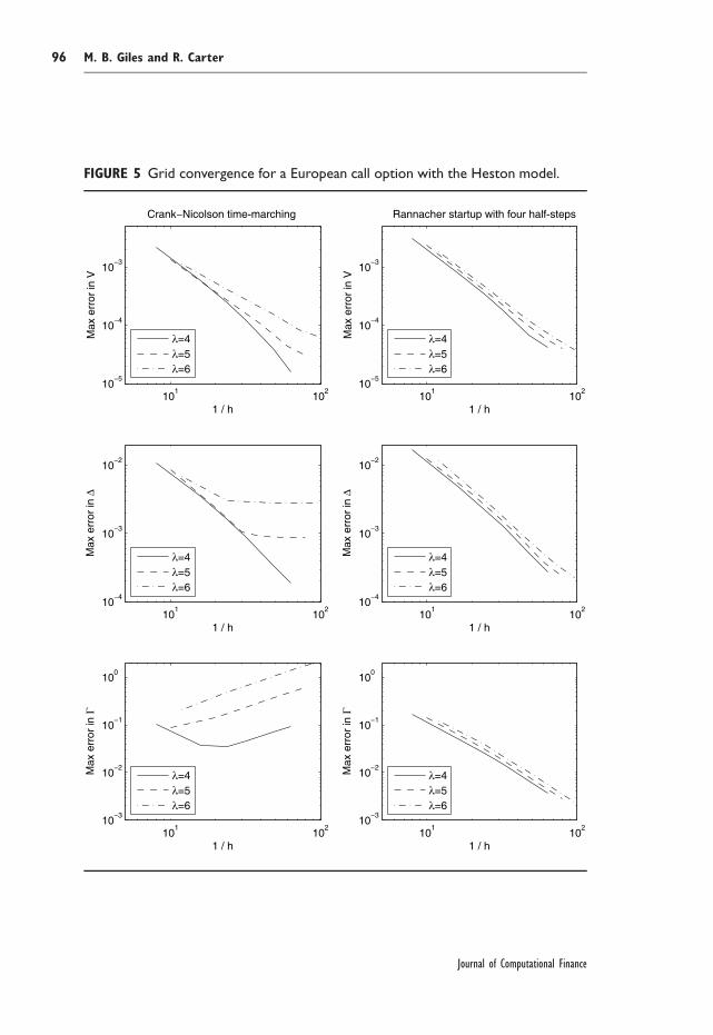
approximations is representative of more realistic multi-factor applications, Fig-ure 5 shows similar results for Heston’s stochastic volatility model (Heston 1993)for which the partial differential equation is

∂V

∂t= rV − rS

∂V

∂S− κ(θ − ν)

∂V

∂ν− 1

2νS2 ∂2V

∂S2− ρωνS

∂2V

∂S∂ν− 1

2ω2ν

∂2V

∂ν2

In two dimensions, the standard Crank–Nicolson method would require thesolution of a very large linear system of equations, making the computationalcost approximately quadratic in the number of grid points. This is avoided here byusing the Alternative Direction Implicit (ADI) method which is a factored approx-imation to the Crank–Nicolson method (Duffy 2006) but has a computationalcost that is proportional to the number of grid points, as in one dimension. Tomaintain second-order accuracy it is necessary to use the Craig–Sneyd treatmentof the cross-derivative term (Craig and Sneyd 1988). The numerical resultsare for a European call option using the following parameter values: r = 0.05,κ = 2, θ = 0.04, ω = 0.25, ρ = −0.5, K = 1, T = 2. The analytic referencesolution is obtained using numerical integration (Kahl and Jackel 2005). The errorplots, which show the maximum error along the line ν = θ , are very similar tothose obtained for the Black–Scholes equation, with the Rannacher timesteppingrestoring second-order accuracy for V , � and �.

The purpose of this paper is to explain the behavior of Rannacher timesteppingby performing a detailed error analysis of a simpler problem, the discretizationof the constant coefficient one-dimensional convection–diffusion equation. Thisreveals that four half-timesteps of backward Euler time-marching is the minimumrequired to recover second-order convergence for these two problems. The use ofmore than four half-timesteps will lead to an increase in the overall error, due tothe lower-order discretization error inherent in the backward Euler discretization,and therefore four half-timesteps can be regarded as optimal.

The approach which is followed is similar to that of Giles (2004), performingan asymptotic analysis of the behavior of the Fourier transform and then using thisto bound the error resulting from the inverse transform (Strang 1986). Numericalresults confirm the sharpness of the error bounds that are derived. A numberof extensions to the analysis are discussed and investigated numerically, andguidance is offered to practitioners wanting to achieve the greatest accuracy for agiven computational cost.



FIGURE 5 Grid convergence for a European call option with the Heston model.

101

102

105

104

103

1 / h

Max

err

or in

V


=4=5=6

101

102

104

103

102

1 / h

Max

err

or in

=4=5=6

101

102

103

102

101

100

1 / h

Max

err

or in

=4=5=6

101

102

105

104

103

1 / h

Max

err

or in

V


=4=5=6

101

102

104

103

102

1 / h

Max

err

or in

=4=5=6

101

102

103

102

101

100

1 / h

Max

err

or in

=4=5=6



There are other ways of obtaining high accuracy implicit solutions. One optionis to follow the approach of Broadie and Detemple (1996) and replace the firsttimestep calculation by the specification of an approximate analytic solution atthe end of the first timestep. This yields the same improvement in accuracyas Rannacher timestepping, provided the approximate solution is sufficientlyaccurate. However, when generalizing this approach to multi-factor models withgeneral payoffs, simple analytic approximations exist for some problems butnot for others. When developing a pricing engine for a large class of models,Rannacher timestepping offers both simplicity and generality.

2 Model problem and discretization

The model problem to be analyzed is the convection–diffusion equation

∂v

∂t+ a

∂v

∂x= ∂2v

∂x2(1)

over −∞ < x < ∞ and 0 < t < 1. The generalization to non-unit diffusivity andterminal times other than t = 1 will be discussed later.

If v(x, t) satisfies this equation subject to the initial data

v(x, 0) = max(x, 0)

then its second derivative

u ≡ ∂2v

∂x2

satisfies the same differential equation subject to the initial data

u(x, 0) = δ(x)

where δ(x) is the Dirac delta function. Defining the Fourier transform pair

u(κ, t) =∫ ∞

−∞u(x, t) e−iκx dx

u(x, t) = 1

2π

∫ ∞

−∞u(κ, t) eiκx dκ

then the Fourier transform of Equation (1) yields

du

dt= −(iaκ + κ2)u

subject to initial data u(κ, 0) = 1. The solution to this is

u(κ, t) = exp(−(iaκ + κ2)t)

and hence

u(x, t) = 1√4πt

exp

(− (x − at)2

4t

)Volume 9/Number 4, Summer 2006


The Crank–Nicolson discretization of Equation (1) on a uniform grid withspacing h and timestep k is

(I + 12D)V n+1

j = (I − 12D)V n

j (2)

where

D = −dδ2x + r

2δ2x, d = k

h2, r = ak

h

with δ2x and δ2x being the usual second difference and central first difference oper-

ators, respectively. The corresponding half-timestep backward Euler discretizationused in the Rannacher startup is

(I + 12D)V

n+1/2j = V n

j (3)

If V nj satisfies these equations with initial data

V 0j = max(xj , 0)

then its divided second difference

Unj = h−2δ2

xV nj

satisfies the same difference equations subject to the Dirac initial data

U 0j = h−1δj,0 =

{h−1, j = 0

0, j �= 0

The objective of the error analysis will be to quantify the error UNj − u(xj , 1) for

N = 1/k.

3 Fourier analysis

Using the mixed discrete/continuous Fourier transform pair (Strang 1986)

Unj = 1

2πh

∫ π

−π

Un(θ) exp(ijθ) dθ

Un(θ) = h

∞∑j=−∞

Unj exp(−ijθ)

the Fourier transform of Equation (2) gives

U n+1m = 1 − 1

2 ir sin θ − 2d sin2 12θ

1 + 12 ir sin θ + 2d sin2 1

2θUn

m

for n ≥ R, where R is the number of initial Crank–Nicolson timesteps replaced by2R half-timesteps of backward Euler time integration, while for n < R the Fourier



transform of Equation (3) gives

U n+1m = 1

(1 + 12 ir sin θ + 2d sin2 1

2θ)2U n

m

These can be combined to give

U n(θ) = zn1(θ)z

min(n,R)2 (θ)U 0(θ)

where

z1(θ) = (1 − 12 ir sin θ − 2d sin2 1

2θ)(1 + 12 ir sin θ + 2d sin2 1

2θ)−1

z2(θ) = (1 − 12 ir sin θ − 2d sin2 1

2θ)−1(1 + 12 ir sin θ + 2d sin2 1

2θ)−1

For the Dirac initial data, U 0 = 1 and hence at the final iteration level N

(assumed to be greater than R)

UNj = 1

2πh

∫ π

−π

zN1 (θ)zR

2 (θ) eijθ dθ (4)

By making the substitutions θ = κh, xj = jh the integral can also be expressed as

UNj = 1

2π

∫ π/h

−π/h

zN1 (κh)zR

2 (κh) eiκxj dκ

This is to be compared to the analytic solution u(x, 1) for which

u(x, 1) = 1

2π

∫ ∞

−∞u(κ, 1) eiκx dκ

withu(κ, 1) = exp(−iaκ − κ2)

Figure 6 plots comparisons between the numerical and analytic solutions to theconvection–diffusion problem with a = 2 at t = 1 for two grid resolutions h = 1/3for the upper half of each figure, and h = 1/6 for the lower half. The timestep ischosen so that λ = k/h = 3/4 in each case. The plots on the left are for Crank–Nicolson without any Rannacher startup, whereas the plots on the right are forR = 2, replacing the first two Crank–Nicolson timesteps by four half-timesteps ofbackward Euler integration.

Looking at the results in physical space (ie, the plots of U and u versus x),the main feature to note is the high-wavenumber error near x = 0 for the Crank–Nicolson time-marching. Its width appears proportional to h, while its magnitudeappears proportional to h−1; this will be confirmed by the asymptotic analysis.

Looking at the comparison in Fourier space (ie, the plots of |U | and |u|versus θ) the main feature to note for the Crank–Nicolson results is that thereappear to be three regions: one on the left of width proportional to h in which



FIGURE 6 Numerical solution for the convection–diffusion equation with a = 2.

4 2 0 2 4

0.2

0

0.2

0.4

0.6

0.8

x

U


uU

0 0.2 0.4 0.6 0.8 1

0

0.2

0.4

0.6

0.8

1

/

Fou

rier

ampl

itude

uU

4 2 0 2 4

0.2

0

0.2

0.4

0.6

0.8

x

U


uU

0 0.2 0.4 0.6 0.8 1

0

0.2

0.4

0.6

0.8

1

/

Fou

rier

ampl

itude

uU

4 2 0 2 4

0.2

0

0.2

0.4

0.6

0.8

x

U

uU

0 0.2 0.4 0.6 0.8 1

0

0.2

0.4

0.6

0.8

1

/

Fou

rier

ampl

itude

uU

4 2 0 2 4

0.2

0

0.2

0.4

0.6

0.8

x

U

uU

0 0.2 0.4 0.6 0.8 1

0

0.2

0.4

0.6

0.8

1

/

Fou

rier

ampl

itude

uU



there is very good agreement between the numerical and analytic solution, oneon the right with a width independent of h in which u is extremely small butU is not, and a central region in which both u and U are small. This separationinto three regions is the basis for the asymptotic analysis, which considers a low-wavenumber range defined by |κ| < h−m, a high-wavenumber range defined byh−r < |κ| and the intermediate range h−m < |κ| < h−r . The constants m and r

satisfy the constraints 0 < m < 13 and 1

2 < r < 1. The reasons for these constraintswill become clear in the asymptotic analysis.

The convergence analysis considers the limit h, k → 0 with λ = k/h held fixed.The reason for this choice of limit is that the truncation error due to the spatialcentral differencing and the Crank–Nicolson time integration O(k2 + h2), andso keeping k = O(h) keeps the spatial and temporal approximation errors of thesame order. We now analyze the Fourier error U − u in each of the three regions.

PROPOSITION 3.1 (Low-wavenumber region) For |κ| < h−m, as h → 0 with λ =k/h held fixed,

UN(κ) − u(κ, 1) = h2 exp(−iaκ − κ2){p(κ, a, λ, R) + O(h(κ3 + κ9))}where

p(κ, a, λ, R) = 16 iaκ3 + 1

12κ4 − 112λ2κ3(ia + κ)3 + 1

4Rλ2κ2(ia + κ)2

PROOF Expressing each variable as a function of h,

θ = κh, N = 1

k= 1

λh, r = aλ, d = λ

h

a Taylor series expansion gives

log UN = N log z1 + R log z2

= −iaκ − κ2 + h2p(κ, a, λ, R) + O(h3(κ3 + κ9))

The restriction that m < 13 ensures that the h2κ6 term and the h3κ9 remainder both

tend to zero as h → 0. Hence,

UN = exp(−iaκ − κ2){1 + h2p(κ, a, λ, R) + O(h3(κ3 + κ9))}and so we obtain the result in the Proposition 3.1.

PROPOSITION 3.2 (High-wavenumber region) For h−r < |κ|, as h → 0 with λ =k/h held fixed,

UN = (−1)N−R h2R

(2λ sin2 12θ)2R

exp

(− 1

λ2 sin2 12θ

)(1 + O(hθ−2))



PROOF z1(θ) can be re-expressed as

z1(θ) = (1 − 12 ir sin θ − 2d sin2 1

2θ)(1 + 12 ir sin θ + 2d sin2 1

2θ)−1

=(

1

2d sin2 12θ

− ir

2dcot 1

2θ − 1

)(1

2d sin2 12θ

+ ir

2dcot 1

2θ + 1

)−1

→ −1 as d → ∞and similarly

z2(θ) = (2d sin2 12θ)−2

(1

2d sin2 12θ

− ir

2dcot 1

2θ − 1

)−1

×(

1

2d sin2 12θ

+ ir

2dcot 1

2θ + 1

)−1

→ −(2d sin2 12θ)−2 as d → ∞

Hence, expressing d and N as functions of h as in the proof of Proposition 3.1,Taylor series analysis gives

log{(−1)N−RUN } = 2R logh

2λ sin2 12θ

− 1

λ2 sin2 12θ

+ O

(h

sin2 12θ

)The restriction that r > 1

2 ensures that the remainder term tends to zero as h → 0,and therefore we obtain the result in the proposition.

PROPOSITION 3.3 (Intermediate region) For h−m < |κ| < h−r , as h → 0 withλ = k/h held fixed, UN(κ) = o(hq), for any q > 0.

PROOF Defining s = sin2 θ2 ,

|z1|2 = (1 − ds)2 + r2s(1 − s)

(1 + ds)2 + r2s(1 − s)

Differentiating, one finds that d|z1|2/ds = 0 when s2 = (d2 − r2)−1. Substitutingr = aλ, d = λ/h, this shows that, as h → 0, |z1| has a maximum at s = 0, 1,and a minimum at s ≈ d−1, corresponding to κ = O(h−1/2) which lies within theintermediate region. Noting that, for any q > 0, the first two Propositions provethat |z1|N = o(hq) at both κ = h−m and κ = h−r , it follows that |z1|N = o(hq)

within the entire intermediate region. Since |zN1 zR

2 | < |z1|N−R, it follows thatUN = o(hq) for any q > 0.

DefiningElow = h2 exp(−iaκ − κ2)p(κ, a, λ, R)

and

Ehigh = (−1)N−R h2R

(2λ sin2 12θ)2R

exp

(− 1

λ2 sin2 12θ

)Journal of Computational Finance


then since Elow � Ehigh in the high-wavenumber region, and Ehigh � Elow in thelow-wavenumber region, the results above can be combined to give

UN(κ) − u(κ, 1) ≈ Elow + Ehigh, |κ| < π/h

The inverse Fourier transform then gives

UNj − u(xj , 1) ≈ Elow

j + Ehighj

where the low-wavenumber error is

Elowj = h2

{Ra2λ2

8√

2N(2)

(xj − a√

2

)− 2a + a3λ2 + 6Raλ2

48N(3)

(xj − a√

2

)+ 1 + 3a2λ2 + 3Rλ2

48√

2N(4)

(xj − a√

2

)− aλ2

32N(5)

(xj − a√

2

)+ λ2

96√

2N(6)

(xj − a√

2

)}with N(m)(x) being the mth derivative of the normal distribution with zero meanand unit variance, and the high-wavenumber error is

Ehighj = (−1)N−Rh2R−1(2λ)−2Rfj

where

fj = h

2π

∫ π/h

−π/h

eiκxj

sin4R 12θ

exp

(− 1

λ2 sin2 12θ

)dκ

= 1

2π

∫ π

−π

eijθ

sin4R 12θ

exp

(− 1

λ2 sin2 12θ

)dθ

= 1

π

∫ π

0

cos jθ

sin4R 12θ

exp

(− 1

λ2 sin2 12θ

)dθ

Ehighj clearly has a width of O(h), and has a maximum magnitude at j = 0 where

xj = 0. This explains the observed behavior in Figure 6. The integral for j = 0can be evaluated analytically (see Appendix A) giving

maxj

|Ehighj | = |Ehigh

0 | = h2R−1(2λ)−2R d2R

dβ2Rerfc(

√β)



where β = λ−2 and erfc(x) is the complementary error function,

erfc(x) = 2√π

∫ ∞

x

e−s2ds

The fact that the low-wavenumber error is O(h2) and the high-wavenumbererror is O(h2R−1) is confirmed by the results in the upper plots of Figure 7which have convergence results for the convection–diffusion equation with a = 2.It can be seen that for the standard Crank–Nicolson time-marching, the resultsexhibit O(h2) convergence until h reaches a sufficiently small value that theO(h−1) high-wavenumber error becomes dominant. The plots show the sensitivedependence of the high-wavenumber error on the value of λ. For large values ofλ, erfc(λ−1) ≈ 1 and so E

highj becomes significant for quite large values of h.

On the other hand, for small values of λ, erfc(λ−1) is extremely small, and soE

highj does not become dominant until h is extremely small. With the Rannacher

startup with four half-timesteps of backward Euler integration (R = 2), the high-wavenumber error is O(h3) and so the low-wavenumber error remains dominantfor all h. The sharpness of the error analysis is demonstrated by the lower plotsthat compare the numerical error with the maximum magnitude of Elow

j and Ehighj .

4 Extensions

4.1 Alternative initial data

The analysis so far has assumed that there is a grid point at x = 0, so the grid isperfectly aligned with the discrete Dirac initial data, but if the grid is not perfectlyaligned care must be taken in representing the initial data, as discussed by Pooleyet al (2003).

If the grid points xj are still taken to be located at jh, but instead of j takinginteger values it is j + α which takes integer values (with 0 < α < 1) then theappropriate discretization of the Dirac initial data is

U 0j =

(1 − α)h−1, j = −α

αh−1, j = 1 − α

0, otherwise

This givesU 0

m = (1 − α) e−iαθm + α ei(1−α)θm

Putting θm = κh, an asymptotic expansion with respect to h gives

U 0m = 1 + O(κ2h2)

which leads to the result that the low-wavenumber error remains second order.It can also be shown that the convergence order of the high-wavenumber error isalso unaffected.



FIGURE 7 Grid convergence for the convection–diffusion equation with a = 2.

100

101

102

106

105

104

103

102

101

1 / h

Max

err

or


=0.4=0.35=0.3=0.25

100

101

102

106

105

104

103

102

101

1 / h

Max

err

or

error, =0.3low-wavenumber errorhigh-wavenumber error

100

101

102

106

105

104

103

102

101

1 / h

Max

err

or


=0.4=0.35=0.3=0.25

100

101

102

106

105

104

103

102

101

1 / h

Max

err

or

error, =0.3low-wavenumber error



TABLE 1 Order of convergence of the high-wavenumber error using Rannachertimestepping with 2R half-timesteps.

V � �

European call 2R + 1 2R 2R − 1Digital call 2R 2R − 1 2R − 2

Although the focus of our analysis so far has been on Dirac initial data, thereare other sets of initial data that are also of interest. One is the first difference ofthe discrete Dirac initial data; this is relevant to the approximation of � for thedigital option. Another is a discrete equivalent of H(x) − 1

2 , where H(x) is theHeaviside step function; this is relevant to the approximation of V for the digitaloption, and � for the European option.

For both of these sets of alternative initial data, the low-wavenumber error willstill be O(h2). However, the high-wavenumber error will be one order worse in thefirst case, O(h2R−2), where R is again the number of Crank–Nicolson timestepsreplaced by two half-timesteps of backward Euler integration, and one order betterin the second case, O(h2R).

Table 1 summarizes the consequences of the analysis and its generalizationsfor the convergence of the high-wavenumber error in computing V , � and �

for European and digital call options. The low-wavenumber error is O(h2) inall cases, and using R = 2 ensures that the high-wavenumber error is also atworst O(h2).

4.2 Diffusion coefficient and terminal time

The model problem that has been analyzed has unit diffusivity, and the error isanalyzed at the terminal time t = 1. Suppose now that the convection–diffusionequation is

∂v

∂t+ a

∂v

∂x= ε

∂2v

∂x2

and the error is to be analyzed at the terminal time t = T . The non-dimensionalization

t∗ = t

T, x∗ = x√

εT, k∗ = k

T, h∗ = h√

εT

λ∗ = k∗

h∗ = k

h

√ε

T= λ

√ε

T, a∗ = a

√T

ε

reduces the more general problem to the one that has already been analyzed.Applying this non-dimensionalization to the Black–Scholes calculations in theintroduction, with ε = 1

2σ 2, then the calculations for λ = 2, 3, 4, 5 correspond toλ∗ ≈ 0.2, 0.3, 0.4, 0.5, respectively.



Having determined that λ∗ is the key non-dimensional parameter, the nextquestion is whether there is an optimal value for this parameter providing themaximum accuracy for a given computational cost. The error analysis gives aleading-order error of the form

E = ah∗2 + bk∗2

while the computational cost is proportional to the product of the number of gridpoints and the number of timesteps, so

C = ch∗−1k∗−1

Hence, for a given computational cost C,

E = h∗k∗(

ah∗

k∗ + bk∗

h∗

)= c

C(aλ∗−1 + bλ∗)

Too small a value for λ∗ gives a large error due to large h∗, while too large avalue of λ∗ gives a large error due to large k∗. This tradeoff is clearly seen inthe results shown in Figure 8. The curves labeled RT2/2 present the maximumerrors for the European and digital call options as a function of λ∗, keepingfixed the computational work by increasing h as k is decreased. The optimumis seen to be around λ∗ = 0.5. The curves labeled CN correspond to the resultsgiven by the standard Crank–Nicolson method. For small values of λ∗ these givemore accurate results because the Rannacher timestepping introduces additionallow-wavenumber errors. However, as λ∗ increases and erfc(1/

√λ∗) is no longer

extremely small, the high-wavenumber error becomes dominant and the Crank–Nicolson error becomes very large.

4.3 Alternative Rannacher treatments

Although Rannacher (1984) originally suggested the approach analyzed here,namely replacing Crank–Nicolson timesteps by two backward Euler half-timesteps, there are other options.

One could replace the Crank–Nicolson timesteps by full timestep backwardEuler approximations, but in this case one would need to replace the firstfour Crank–Nicolson timesteps to get the same improvement in the order ofconvergence, and the larger timestep in the backward Euler time integration wouldincrease the low-wavenumber error.

A better option is to replace the first Crank–Nicolson timestep by four quarter-timesteps of backward Euler time integration. This gives the same desiredimprovement in the order of convergence, but with a reduced low-wavenumbererror. The curves labeled RT1/4 in Figure 8 present the results obtained in thisway. The results are clearly superior in all cases except perhaps for the digitaloption � for which there is a second-order high-wavenumber error in addition tothe second-order low-wavenumber error, and RT1/4 does not eliminate the high-wavenumber error as effectively as RT2/2.



FIGURE 8 Comparison of four numerical methods: Crank–Nicolson (CN), Ran-nacher timestepping with four half-timesteps (RT2/2) with four quarter-timesteps(RT1/4), and with four quarter-timesteps and non-uniform timesteps (variable).

101

100

104

103

*

Max

err

or in

V

European call

CNRT2/2RT1/4variable

101

100

104

103

102

*

Max

err

or in


101

100

103

102

101

*

Max

err

or in


101

100

104

103

*

Max

err

or in

V

Digital call


101

100

103

102

*

Max

err

or in


101

100

102

101

100

*

Max

err

or in




4.4 Non-uniform timesteps

Another possibility is not to use uniform timesteps, but instead use smallertimesteps initially. Given the existence of an optimal value for λ∗, one wayof choosing the timestep might be to keep fixed the value of λ∗(t) based onthe current time t rather than the final time T . This requires k ∝ √

t which isaccomplished by defining

kn = tn+1 − tn, tn = n2

N2T

so that t0 = 0, tN = T and kn ∝ n ∝ √tn.

The curves labeled “variable” in Figure 8 show that this does not produce verygood results. The problem is that, as with the basic Crank–Nicolson method, theerror rises very sharply when λ∗ increases. This is because the very small initialtimesteps greatly reduce the effectiveness of the backward Euler smoothing of thehigh-wavenumber error. In fact, additional results, backed by numerical analysis,show that one does not obtain second-order convergence in any of the cases. Thiscontrasts slightly with the results of Forsyth and Vetzal (2002) who found that forAmerican options this variable timestep gives second-order convergence for theoption value whereas the uniform timestep does not, probably due to its inadequateresolution of the initial behavior of the exercise boundary.

4.5 Richardson extrapolation

The final extension to be considered is Richardson extrapolation (Dahlquist andBjörck 1974; Geske and Johnson 1984). Given that the leading-order term in thelow-wavenumber error is of the form

Elowh = ah2 + bk2

then if one performs calculations with spacing 2h and h, keeping the ratio λ fixed,then

4Elowh − E2h

low = 0

Hence, the extrapolated solution

Uext = 43Uh − 1

3U2h

will have a low-wavenumber error that does not have a leading second-order term.Figure 9 shows the improved accuracy of this extrapolated solution. Further

numerical analysis reveals that the next order low-wavenumber error term is due tothe Rannacher time-marching and is proportional to Rk3. This explains the third-order convergence that is apparent in some of the plots for λ∗ = 0.5. For λ∗ = 0.2,k3 is sufficiently small so that the third-order error is relatively insignificant. Thesecond-order convergence of the digital option � is due to the high-wavenumbererror which is second order in this case and is not cancelled by the extrapolationprocedure.



FIGURE 9 Convergence comparison for Rannacher time-marching using fourquarter-timesteps, with and without Richardson extrapolation.

101

102

103

108

106

104

102

1 / h

Max

err

or in

V

European call

*=0.2*=0.2 (ext)*=0.5*=0.5 (ext)

101

102

103

106

104

102

100

1 / h

Max

err

or in

*=0.2*=0.2 (ext)*=0.5*=0.5 (ext)

101

102

103

106

104

102

100

1 / h

Max

err

or in

*=0.2*=0.2 (ext)*=0.5*=0.5 (ext)

101

102

103

108

106

104

102

1 / h

Max

err

or in

V

Digital call

*=0.2*=0.2 (ext)*=0.5*=0.5 (ext)

101

102

103

106

104

102

100

1 / h

Max

err

or in

*=0.2*=0.2 (ext)*=0.5*=0.5 (ext)

101

102

103

106

104

102

100

1 / h

Max

err

or in

*=0.2*=0.2 (ext)*=0.5*=0.5 (ext)



5 Conclusions

In this paper we have analyzed the convergence of Crank–Nicolson approxima-tions of the one-dimensional convection–diffusion equation, with and without theRannacher startup procedure in which an initial R Crank–Nicolson timesteps areeach replaced by two half-timesteps of backward Euler integration. The analysisproves, and numerical results confirm, that there is a low-wavenumber error ofO(h2), and a high-wavenumber error of O(h2R−1). Hence R = 2 is the minimumto give O(h2) convergence, and it in general it is the optimum since larger valueswill increase the low-wavenumber error.

In considering extensions to this analysis and its relevance to Black–Scholesapplications, it was shown that it is better to replace just the first Crank–Nicolson timestep by four quarter-timesteps of backward Euler time integration.This reduces the low-wavenumber error introduced by the Rannacher startup. Inaddition, the accuracy is maximized for a given computational cost by choosingthe uniform timestep k and grid spacing h so that

λ∗ = k

h

√σ 2

2T

lies between 0.5 and 1.0. Using a variable timestep does not improve the accuracy,and in fact spoils the second-order convergence. The final comment is thatnumerical results show that very significant improvement in accuracy (or decreasein computational cost) can be achieved using Richardson extrapolation.

Appendix A Evaluation of the integral

Consider the integral

I0 = 1

π

∫ π

0exp

(− 1

λ2 sin2 12θ

)dθ

Making the substitutions t = cot 12θ and α = λ−1, one obtains

I0 = 2

π

∫ ∞

0

1

t2 + 1exp(−α2(t2 + 1)) dt

and hencedI0

dα= −4α

π

∫ ∞

0exp(−α2(t2 + 1)) dt = − 2√

πexp(−α2)

Since I0 → 0 as α → ∞, integration gives

I0 = 2√π

∫ ∞

λ−1exp(−s2) ds ≡ erfc(λ−1)

where erfc(x) is the complementary error function.Switching to a new variable β = λ−2 = α2, then I0(β) = erfc(

√β), and

IR(β) ≡ 1

2π

∫ π

−π

1

(sin2 12θ)2R

exp

(− β

sin2 12θ

)dθ = d2RI0

dβ2R



REFERENCES

Broadie M., and Detemple, J. (1996). American option valuation: new bounds, approximations,and a comparison of existing methods. Review of Financial Studies 9(4), 1211–1250.

Craig, I. J. D., and Sneyd, A. D. (1988). An alternating-direction implicit scheme for parabolicequations with mixed derivatives. Computers & Mathematics with Applications 16(4), 341–350.

Dahlquist, G., and Björck A. (1974). Numerical Methods. Prentice-Hall, Englewood Cliffs, NJ.

Duffy, D. (2006). Finite Difference Methods in Financial Engineering: A Partial DifferentialEquation Approach. Wiley.

Forsyth, P. A., and Vetzal, K. R. (2002). Quadratic convergence for valuing American optionsusing a penalty method. SIAM Journal on Scientific Computing 23(6).

Geske, R., and Johnson, H. E. (1984). The American put option valued analytically. Journal ofFinance 39(5), 1511–1524.

Giles, M. B. (2004). Sharp error estimates for a discretisation of the 1D convection/diffusionequation with Dirac initial data. Technical Report NA04/17, Oxford University ComputingLaboratory.

Heston, S. I. (1993). A closed-form solution for options with stochastic volatility withapplications to bond and currency options. Review of Financial Studies 6, 327–343.

Ikonen, S., and Toivanen, J. (2004). Pricing American options using LU decomposition. Tech-nical Report B 4/2004, Department of Mathematical Information Technology, University ofJyväskylä.

Kahl, C., and Jäckel, P. (2005). Not-so-complex logarithms in the Heston model. WilmottSeptember.

Pooley, D. M., Forsyth, P. A., and Vetzal, K. R. (2003a). Numerical convergence propertiesof option pricing PDEs with uncertain volatility. IMA Journal of Numerical Analysis 23,241–267.

Pooley, D. M., Vetzal, K. R., and Forsyth, P. A. (2003b). Convergence remedies for non-smoothpayoffs in option pricing. Journal of Computational Finance 6(4).

Raahauge, P. (2004). Higher-order finite element solutions of option prices. Working PaperSeries No. 184, University of Aarhus Center for Analytical Finance.

Rannacher, R. (1984). Finite element solution of diffusion problems with irregular data.Numerische Mathematik 43, 309–327.

Richtmyer, R. D., and Morton, K. W. (1967). Difference Methods for Initial-Value Problems,2nd edn. Wiley-Interscience. Reprint (1994), Krieger Publishing Company, Malabar.

Strang, G. (1986). Introduction to Applied Mathematics. Wellesley-Cambridge Press, Wellesley,MA.

Wilmott P., Howison, S., and Dewynne, J. (1995). The Mathematics of Financial Derivatives.Cambridge University Press, 1995.

Zvan, R., Forsyth, P. A., and Vetzal, K. R. (2003). Negative coefficients in two factor optionpricing models. Journal of Computational Finance 7(1).


Convergence analysis of Crankâ€“Nicolson and Rannacher time

Documents

Transcript of Convergence analysis of Crankâ€“Nicolson and Rannacher time