Noname manuscript No.(will be inserted by the editor)

Convergence analysis of a Galerkin boundary elementmethod for electromagnetic resonance problems

Gerhard Unger

Received: date / Accepted: date

Abstract In this paper a convergence analysis of a Galerkin boundary elementmethod for resonance problems arising from the time harmonic Maxwell’s equa-tions is presented. The cavity resonance problem with perfect conducting boundaryconditions and the scattering resonance problem for impenetrable and penetrablescatterers are treated. The considered boundary integral formulations of the reso-nance problems are eigenvalue problems for holomorphic Fredholm operator-valuedfunctions, where the occurring operators satisfy a so-called generalized Garding’sinequality. The convergence of a conforming Galerkin approximation of this kind ofeigenvalue problems is in general only guaranteed if the approximation spaces ful-fill special requirements. We use recent abstract results for the convergence of theGalerkin approximation of this kind of eigenvalue problems in order to show thattwo classical boundary element spaces for Maxwell’s equations, the Raviart–Thomasand the Brezzi–Douglas–Marini boundary element spaces, satisfy these requirements.Numerical examples are presented, which confirm the theoretical results.

Keywords Electromagnetic resonance problem · Boundary element method ·Scattering resonances

Mathematics Subject Classification (2010) 65N25 · 65N38 · 65N12 · 78M15

1 Introduction

The numerical solution of electromagnetic resonance problems is an important taskin different fields of engineering and technology. In this paper we consider for a givenbounded, simply connected Lipschitz domain Ωi ⊂ R3 the cavity resonance problem

The author acknowledges support from the Austrian Science Fund (FWF): P31264

Gerhard UngerInstitut fur Angewandte Mathematik, Technische Universitat Graz, Steyrergasse 30, 8010 Graz,Austria,E-mail: gerhard.unger@tugraz.at

and the scattering resonance problem for an impenetrable and a penetrable scattererarising from the time harmonic Maxwell’s equations with a time variation of the forme−iωt. It is assumed that the exterior domain Ωe := R3 \Ωi is connected.

The cavity resonance problem, usually referred to as interior resonance problem,is given as follows: Find κ ∈ C and Ei ∈ H(curl;Ωi), Ei 6= 0, such that

curl curl Ei − κ2Ei = 0 in Ωi,

div(εEi) = 0 in Ωi,

Ei × n = 0 on Γ := ∂Ωi,

(1)

where κ = ω√εµ is the wavenumber, ω is the angular frequency, ε is the electric per-

mittivity, µ is the magnetic permeability, and n is the unit normal vector field on theboundary Γ pointing into the exterior domain Ωe. For the cavity resonance problemand the resonance problem for the impenetrable scatterer we assume throughoutthis paper that ε > 0 and µ > 0 are constant. This assumption implies that the res-onances of the interior resonance problem (1) are real [27, Thm. 4.18] and non-zero.

The scattering resonance problem for the impenetrable scatterer, which is usuallyreferred to as exterior resonance problem, is formulated in Ωe and is given as follows:Find κ ∈ C and Ee ∈ Hloc(curl;Ωe), Ee 6= 0, such that:

curl curl Ee − κ2Ee = 0 in Ωe, (2a)

div(εEe) = 0 in Ωe, (2b)

Ee × n = 0 on Γ, (2c)

Ee is “outgoing”. (2d)

As radiation condition in (2d) we impose that each Cartesian component of Ee hasoutside of any ball Br0 := x : ‖x‖ < r0 which contains Ωi an expansion in terms

of the spherical Hankel functions of the first kind h(1)n of the form

(Ee(x))[j] =∞∑n=0

n∑m=−n

a(j)n,mh

(1)n (κr)Ymn

(x

‖x‖

)(3)

for r = ‖x‖ > r0 and j ∈ 1, 2, 3, where Ymn are the spherical harmonics. If κ is suchthat 0 ≤ arg κ < π, then the radiation condition (3) for a solution E ∈ Hloc(curl;Ωe)of Maxwell’s equations in Ωe is equivalent to that the Cartesian components of Esatisfy the Sommerfeld radiation condition [11, Thm. 2.15]. The latter conditionis again for 0 ≤ arg κ < π equivalent to that E satisfies the Silver-Muller radiationcondition [11, Thm. 6.8]. The Silver-Muller radiation condition is usually imposed forscattering problems for wavenumbers κ with 0 ≤ arg κ < π. But it is well known thatfor wavenumbers with negative imaginary part the Silver-Muller radiation conditiondoes not not correctly characterize outgoing waves, see e. g., [28, Sect. 1]. Sincethe resonances of the exterior resonance problem (2) have negative imaginary part,instead of the Silver-Muller radiation condition the radiation condition (3) is used.

The definition of the scattering resonance problem for the penetrable scattererwill be given in Section 5. For this kind of resonance problem we will allow com-plex and frequency-dependent permittivities and permeabilities. Such configurationsoccur for example in the field of plasmonics or in the context of metamaterials.

2

Boundary integral formulations and boundary element methods have been con-sidered for different kinds of electromagnetic resonance problems. Examples are theinterior resonance problem [13,37], the interior transmission eigenvalue problem [12,22] or the resonance problem for the penetrable scatterer [24,26,35], to mention justa few. A rigorous convergence analysis of the boundary element approximations ofsuch kind of resonance problems has not been provided so far.

The presented numerical analysis in this paper is based on the classical the-ory of the regular approximation of eigenvalue problems for holomorphic Fredholmoperator-valued functions [17,18]. This theory has already been applied to boundaryintegral formulations of acoustic resonance problems [33] and to coupled FEM-BEMformulations of vibro-acoustic resonance problems [20]. For these cases sufficient con-ditions for the convergence of conforming Galerkin approximations follow from thefact that the occurring operators satisfy a standard Garding’s inequality. For electro-magnetic resonance problems the occurring boundary integral operators satisfy onlya generalized Garding’s inequality. In such a case additional properties of the approx-imation spaces are required in order to guarantee convergence. In [15,16] sufficientconditions for the convergence of a conforming Galerkin approximation for such kindof eigenvalue problems are derived in an abstract setting. In this paper we show thatthese conditions are satisfied for the Galerkin approximation of the proposed bound-ary integral formulations of the considered electromagnetic resonance problems whenclassical boundary elements of Raviart–Thomas or Brezzi–Douglas–Marini type areused.

The rest of the paper is organized as follows: in the next section we introducethe boundary integral formulation for the interior and exterior resonance problemand collect the basic properties of the occurring boundary integral operators. InSection 3 we provide abstract convergence results for the Galerkin approximationof eigenvalue problems for holomorphic Fredholm operator-valued functions, wherewe assume that the occurring operators satisfy a generalized Garding’s inequality.We specify for this case sufficient conditions such that the classical convergenceresults are valid. The abstract results of Section 3 are then applied in Section 4 toa Galerkin approximation of the boundary integral formulation of the interior andexterior resonance problem. In Section 5 a boundary integral formulation for thescattering resonance problem for a penetrable scatterer is analyzed and sufficientconditions on the material parameter are given such that convergence of boundaryelement methods are guaranteed. Numerical examples are presented in Section 6,which confirm the theoretical results.

2 Boundary integral formulation of the interior and exterior resonanceproblem

In this section we introduce and analyze the boundary integral formulation for theinterior and exterior resonance problem (1) and (2). The main references for thedefinitions and properties of the occurring boundary integral operators are [8,9]. Notethat the notations in the present paper only partially coincides with the notationsin [8,9].

3

2.1 Trace spaces

In this subsection we summarize the properties of the trace spaces which we need forthe analysis of the boundary integral formulations of the resonance problems. For adetailed presentation of the trace spaces related to Maxwell’s equations for Lipschitzdomains we refer to [7].

Let Ω be a Lipschitz domain. We denote by Hs(Ω), s ∈ R, and by Ht(∂Ω),t ∈ [−1, 1], the standard Sobolev spaces of scalar functions on the domain Ω andits boundary ∂Ω, cf. [25]. The vector-valued counterparts Hs(Ω) := (Hs(Ω))3 and

Ht(∂Ω) :=(Ht(∂Ω)

)3are written in bold letters. Throughout the paper we use

bold letters for vector-valued functions. Further, we define

Hsloc(Ω) := F : Ω → C3 | ∀ϕ ∈ C∞0 (R3) : ϕF ∈ Hs(Ω), s ≥ 0,

H(curl, Ω) := F ∈ (L2(Ω))3 | curl F ∈ (L2(Ω))3

Hloc(curl, Ω) := F ∈ L2loc(Ω) | curl F ∈ L2

loc(Ω),

where L2loc(Ω) := H0

loc(Ω).In the following let us consider the domains Ωi and Ωe = R3 \Ωi as introduced

in Section 1. For smooth functions Ei/e ∈ E|Ωi/e : E ∈ (C∞0 (R3))3 we define the

interior/exterior tangential trace operators γi/eτ and π

i/eτ by

γi/eτ Ei/e := E

i/e|Γ × n and πi/e

τ Ei/e := n×(E

i/e|Γ × n

).

The operators γi/eτ and π

i/eτ can be extended for s ∈ (0, 1) to continuous operators

γiτ : Hs+1/2(Ωi)→ Vs

γ := γiτ (Hs+1/2(Ωi)), γe

τ : Hs+1/2loc (Ωe)→ Vs

γ

πiτ : Hs+1/2(Ωi)→ Vs

π := πiτ (Hs+1/2(Ωi)), πe

τ : Hs+1/2loc (Ωe)→ Vs

π

where Vsγ and Vs

π are endowed with the norms

‖u‖Vsγ

:= infE∈Hs+1/2(Ωi)

‖E‖Hs+1/2(Ωi) : γiτ (E) = u,

‖s‖Vsπ

:= infE∈Hs+1/2(Ωi)

‖E‖Hs+1/2(Ωi) : πiτ (E) = s.

The dual space of Vsγ and Vs

π, s ∈ (0, 1), are denoted by V−sγ and V−sπ , respectively.For s = 0 we set V0

γ = V0π := L2

τ (Γ ) := u ∈ L2(Γ ) : u · n = 0, where L2τ (Γ ) acts

as pivot space for V−sγ and Vsγ as well as for V−sπ and Vs

π. Finally, we define thespace

H−1/2(divΓ, Γ ) := u ∈ V− 1

2π : divΓ u ∈ H−

12 (Γ )

endowed with the graph norm ‖u‖2H−1/2(divΓ,Γ ) := ‖u‖2V− 1

2π

+ ‖divΓ u‖2H−

12 (Γ )

. The

space H−1/2(divΓ, Γ ) is a Hilbert space and the tangential trace operators γiτ and

γeτ can be extended such that

γiτ : H(curl;Ωi)→ H−1/2(divΓ, Γ ), γe

τ : Hloc(curl;Ωe)→ H−1/2(divΓ, Γ ),

4

are continuous, surjective and possess a continuous right inverse [7, Thm. 4.1]. Inthe sequel we will use the shorthand notation

V := H−1/2(divΓ, Γ ).

The antisymmetric pairing

〈u, s〉τ :=

∫Γ

(u× n) · s ds, u, s ∈ L2t (Γ )

can be extended to V such that V becomes its own dual [9, Thm. 3.3], i.e., thereexists a linear and isometric isomorphism J× : V→ V′ such that

〈u, s〉τ = (J×u)(s) for all u, s ∈ V.

The operator J× : V → V′ is the extension of the mapping J× : L2τ (Γ ) → L2

τ (Γ )defined by J×(u) := u × n, see [9, Thm. 3.3]. Since V is a Hilbert space we canidentify the pairing 〈·, ·〉τ with the inner product (·, ·)V by

〈u, s〉τ = (JVJ×u, s)V, u, s ∈ V, (4)

where JV : (H−1/2(divΓ, Γ ))′ → H−1/2(divΓ, Γ ) is a linear, isometric isomorphism.

As additional traces we introduce the traces γi/eN := γ

i/eτ curl. The mappings

γiN : H(curl2;Ωi) 7→ V and γe

N : Hloc(curl2;Ωe) 7→ V are linear and continuous [8],where

H(curl2;Ωi) := F ∈ H(curl, Ωi) | curl curl F ∈ (L2(Ω))3,

Hloc(curl2;Ωe) := F ∈ Hloc(curl, Ωe) | curl curl F ∈ L2loc(Ωe).

2.2 Derivation and analysis of the boundary integral formulation

The boundary integral formulation of the resonance problems (1) and (2) is basedon the Stratton-Chu representation formula for the solution of Maxwell’s equations.For exterior problems this formula is in the literature only considered for wavenum-bers with non-negative imaginary part and together with the Silver-Muller radiationcondition; see, e.g., [8, Sect. 4], [21, Thm. 5.49], [29, Sect. 5.5]. For wavenumberswith negative imaginary part the Stratton-Chu representation formula is also validif instead of the Silver-Muller radiation condition the radiation condition (3) is im-posed. This can be shown in the same way as it is done for positive wavenumbersin [8, Sect. 4, p. 95–97] by considering the Cartesian components of the solutionof Maxwell’s equations, which have to satisfy the scalar Helmholtz equation. Therepresentation formula for outgoing solutions of the scalar Helmholtz equation isalso valid for wavenumbers with negative imaginary part [34, Appendix, Cor. 6.5]and therefore the Stratton-Chu representation formula is also valid for wavenumberswith negative imaginary part for exterior problems. We consider the Stratton-Churepresentation formula in following compact form as in [8, Sect. 4]: any solution E

5

of Maxwell’s equations in Ωi ∪Ωe with wavenumber κ ∈ C \ 0 which satisfies theradiation condition (3) is given by

E(x) =(

ΨDL(κ)(γiτ E−γe

τ E))(x)+

(ΨSL(κ)(γi

N E−γeN E)

)(x), x ∈ Ωi∪Ωe, (5)

where

(ΨSL(κ)u) (x) := (ΨA(κ)u) (x) +1

κ2∇ (ΨV(κ) divΓ u) (x), x ∈ Ωi ∪Ωe,

is the Maxwell single layer potential and where

(ΨDL(κ)u) (x) := curl (ΨA(κ)u) (x) x ∈ Ωi ∪Ωe,

is the Maxwell double layer potential. Here, ΨA(κ) and ΨV(κ) are the vectorialand scalar single layer potentials related to the Helmholtz equation, which have theintegral representations

(ΨA(κ)u) (x) :=

∫Γ

u(y)Eκ(x− y)dsy, (ΨV(κ)φ) (x) :=

∫Γ

φ(y)Eκ(x− y)dsy

with Eκ(x) = exp(iκ‖x‖)/4π‖x‖.Let (κi,Ei) be an eigenpair of (1) and let us extend Ei in Ωe by zero, then the

Stratton-Chu representation formula (5) gives((ΨSL(κi))(γi

N Ei))

(x) =

Ei(x), x ∈ Ωi,

0, x ∈ Ωe.(6)

If (κe,Ee) is an eigenpair of (2) and if we extend Ee by zero in Ωi, then we have

−(

(ΨSL(κe))(γeN Ee)

)(x) =

0, x ∈ Ωi,

Ee(x), x ∈ Ωe.(7)

We consider a boundary integral formulation of the eigenvalue problems (1) and (2)in terms of the single layer boundary integral operator S(κ) which is defined by

S(κ)u := 12

(γiτ ΨSL(κ) + γe

τ ΨSL(κ))

u, u ∈ V.

The operator S(κ) : V→ V is linear and continuous [8, Cor. 2] and it holds S(κ) =γiτ ΨSL(κ) = γe

τ ΨSL(κ) [8, Thm. 7]. Further, we have the following representation[8, Eq. (31)]

〈S(κ)u, r〉τ = −〈r,A(κ)u〉τ +1

κ2〈divΓ r, V (κ) divΓ u〉∓ 1

2, A(κ) := γi

τ ΨA(κ). (8)

Here V (κ) is the single layer operator of the Helmholtz equation and the pairing

〈·, ·〉∓ 12

denotes the duality pairing of H−12 (Γ ) and H

12 (Γ ). By applying the tan-

gential trace to (6) and (7) we see that (κi,Ei) and (κe,Ee) satisfy the followingboundary integral equation

S(κi/e)(γi/eN Ei/e) = 0. (9)

6

As boundary integral formulation of the eigenvalue problems (1) and (2) we considerthe following eigenvalue problem: Find κ ∈ C \ 0 and u ∈ V \ 0 such that:

S(κ)u = 0. (10)

Note that this eigenvalue problem is nonlinear with respect to the eigenvalue pa-rameter κ. The eigenvalue problem (10) is referred to as eigenvalue problem for theoperator-valued function S : C \ 0 → B(V,V). Here B(V,V) denotes the spaceof linear and bounded operators mapping from V into V. The equivalence of theeigenvalue problem (10) with the interior and exterior resonance problem (1) and (2)is specified next.

Proposition 2.1 The following assertions hold true:

(i) Suppose that (κ,E) is an resonance pair either of the interior resonance prob-

lem (1) or of the exterior resonance problem (2). Then (κ, γi/eN E) is an eigen-

pair of the eigenvalue problem (10).(ii) Let (κ,u) be an eigenpair of the eigenvalue problem (10). If κ is real, then it

is a resonance of the interior resonance problem (1) and (ΨSL(κ)u)|Ωi is acorresponding resonance function. Otherwise, κ is a resonance of the exteriorresonance problem (2) and (ΨSL(κ)u)|Ωe is a corresponding resonance function.

Proof. The assertion (i) has been already shown, see (9). Suppose now that (κ,u)is an eigenpair of (10). We define E = ΨSL(κ)u in Ωi ∪ Ωe. Then γi

τ E = γeτ E =

S(κ)u = 0. It remains to show that E|Ωi 6= 0 if κ ∈ R, and E|Ωe 6= 0 if κ ∈ C \ R.First we consider the case that κ ∈ R. Then E|Ωe = 0 because of the unique

solvability of the related exterior boundary value problem [21, Cor. 5.63]. From thiswe get γe

N E = 0 and the jump relation γeN ΨSL(κ)u− γi

N ΨSL(κ)u = −u [8, Thm. 7]implies E|Ωi 6= 0.

Suppose now that κ is non-real. Then E|Ωi = 0 because otherwise (κ,E|Ωi) wouldbe an interior resonance pair which is not possible since all interior resonances arereal [27, Thm. 4.18]. From the jump relation of the single layer potential we getγe

N E = u. Hence we have E|Ωe 6= 0.

For the analysis of the eigenvalue problem (10) and its Galerkin approximationit is essential that the single layer boundary integral operator S(κ) satisfies a gener-alized Garding’s inequality in V for all wavenumbers κ ∈ C \ 0. This property isbased on the direct sum decomposition

V = X ⊕N , (11)

where X and N are closed subspaces of V with X ⊂ V −12

π and N = (ker divΓ) ∩ V[9, Thm. 3.4]. We denote by R and Z the associated continuous projectors onto Xand N , respectively. An equivalent norm in V is given by

(‖Z ·‖2V− 1

2π

+ ‖divΓ R ·‖2H−

12 (Γ )

)1/2, (12)

see [9, Thm. 3.4]. Further, we define the operator

Θ := R−Z : V→ V, (13)

which is by construction an isomorphism.

7

Lemma 2.1 Let κ ∈ C \ 0. There exist a compact operator C(κ) : V → V, anisomorphism T(κ) : V → V and an α(κ) > 0 such that the following generalizedGarding’s inequality is satisfied

Re〈(S(κ) + C(κ))u, β(κ)T(κ)u〉τ ≥ α(κ)‖u‖2V for all u ∈ V, (14)

where

T(κ) := κ−1T(κ), T(κ) :=

Θ for Re(κ) 6= 0,

I for Re(κ) = 0,

β(κ) := sgn(Re(κ)) for Re(κ) 6= 0, and β(κ) := − sgn(Im(κ))i for Re(κ) = 0.

Proof. The assertion has been proven for positive wavenumbers e. g. in [6, Thm. 5],[8, Lem. 10], [9, Thm. 5.4]. Using the same arguments as in [6,8,9] an extension toκ ∈ C \ 0 is straightforward. We want to mention that the assertion follows alsofrom Prop. 5.1 below when setting u = (0,u) in (49).

Next, we show that the mapping S : C\0 → B(V,V), κ 7→ S(κ), is holomorphic,i.e., the derivative d

dκ S(κ0) := limκ→κ0

1κ−κ0

(S(κ)− S(κ0)) exists as operator inB(V,V) for each κ0 ∈ C \ 0.

Lemma 2.2 The mapping S : C \ 0 → B(V,V), κ 7→ S(κ), is holomorphic.

Proof. It is sufficient to show that the mapping

κ 7→ 〈S(κ)u, r〉τ

is holomorphic as mapping from C\0 into C for all u, r of a dense subspace of V, seeTheorem III.3.12 in [19] and the remark following it. Let us choose γi

τ ((C∞0 (R3))3)as dense subspace of V. Then we can use the following integral representation of thepairing 〈·, ·〉τ and of the boundary integral operator S(κ) [8, Eq. 32]:

〈S(κ)u, r〉τ = −∫Γ

∫Γ

eiκ‖x−y‖

4π‖x− y‖u(x) · r(y)dsydsx

+1

κ2

∫Γ

∫Γ

eiκ‖x−y‖

4π‖x− y‖ divΓ u(x) divΓ r(y)dsydsx. (15)

Hence, it is sufficient to show that both terms on the right hand side in (15) areholomorphic in κ on C\0. We give a proof for the first term only, since the secondterm can be treated analogously. We divide the proof in two steps.

Step 1: Consider for a fixed κ ∈ C the series expansion of the kernel

∫Γ

∫Γ

eiκ‖x−y‖

4π‖x− y‖u(x) · r(y)dsydsx

=

∫Γ

∫Γ

∞∑n=0

(iκ)n

4πn!‖x− y‖n−1u(x) · r(y)dsydsx. (16)

8

We show that the order of integration and summation can be interchanged by usingLebegue’s dominated convergence theorem. Let

fn(κ,x,y) := (4πn!)−1(iκ)n‖x− y‖n−1u(x) · r(y).

Obviously∑Nn=0 fn(κ,x,y) converges pointwise almost everywhere on Γ ×Γ to the

kernel on the left hand side in (16) as N →∞. Further, for R := maxx,y∈Γ ‖x− y‖we have ∣∣∣∣∣

N∑n=0

fn(κ,x,y)

∣∣∣∣∣ ≤(

1

4π‖x− y‖ +N∑n=1

(iκ)n

4πn!Rn−1

)‖u‖∞‖r‖∞

≤

(1

4π‖x− y‖ +e|ikR|

4πR

)‖u‖∞‖r‖∞ =: g(κ,x,y)

Since g(κ,x,y) is integrable on Γ×Γ the order of integration and summation in (16)may be interchanged.

Step 2: Define for κ ∈ BK(0), K > 0,

hn(κ) :=

∫Γ

∫Γ

fn(κ,x,y)dsydsx.

We have

|hn(κ)| ≤

M0 := |Γ |‖V (0)‖B(H−1/2(Γ ),H1/2(Γ ))‖u‖∞‖r‖∞ for n = 0,

Mn := |Γ |24πR

|KR|nn! ‖u‖∞‖r‖∞ for n > 0,

where V (0) is the single layer boundary integral operator of the Laplace equation,see [32, Sect. 6.2]. Obviously,

∑∞n=0Mn is convergent. Hence, by the Weierstrass

M-test it follows that the series∑∞n=0 hn(κ) converges absolutely and uniformly on

BK(0) to a limit function h(κ). Since∑Nn=0 hn(κ) is a polynomial in κ and therefore

holomorphic in κ the uniform convergence of∑Nn=0 hn(κ) implies that the limit

function h(κ) is holomorphic on BK(0). From the first part of the proof we get

h(κ) =

∫Γ

∫Γ

eiκ‖x−y‖

4π‖x− y‖u(x) · r(y)dsydsx,

which shows that the first term on the right hand side in (15) defines a holomorphicfunction on C. Analogously, the holomorphy of the second term can be shown.

3 Galerkin approximation of eigenvalue problems for holomorphicFredholm operator-valued functions

In this section we provide abstract convergence results for the Galerkin approxi-mation of eigenvalue problems for holomorphic Fredholm operator-valued functionswhere we assume that the occurring operators satisfy a generalized Garding’s in-equality. We specify for this case sufficient conditions such that the classical conver-gence results for the approximation of eigenvalue problems for holomorphic Fredholm

9

operator-valued functions as given in [17,18] can be applied. Our analysis is basedon results on the approximation of non-coercive operators [4] and on recent resultson the regular approximation of operators which satisfy a generalized Garding’s in-equality [15,16].

The results of this section build the abstract framework which we will utilizein order to show the convergence of the boundary element method for the approx-imation of the interior and exterior resonance problem as well as of the resonanceproblem for the penetrable scatterer.

3.1 Assumptions on the eigenvalue problem

Let V be a Hilbert space and suppose that V is equipped with a conjugation, i. e.,with a continuous, unary operation v 7→ v satisfying

u+ v = u+ v, αu = α u, and v = v,

for all u, v ∈ V and α ∈ C. We denote by (·, ·)V the inner product in V and considerin addition a bilinear form 〈·, ·〉V : V × V → C with the property

〈u, v〉V = (Ju, v)V for all u, v ∈ V, (17)

where J ∈ B(V, V ) is a given isomorphism. Further, we assume that there exists adirect sum decomposition V = X ⊕N which is stable, i. e., there exists a constantc > 0 such that for all vX ∈ X and vN ∈ N the inequality

(‖vX‖V + ‖vN‖V ) ≤ c(‖vX + vN‖V ) (18)

is satisfied. We define the operator Θ : V → V by

Θ : v = vX + vN 7→ vX − vN , vX ∈ X, vN ∈ N. (19)

Note that Θ is an isomorphism and that Θ ∈ B(V, V ) since the decompositionV = X ⊕N is stable.

Let Λ ⊂ C be an open and connected subset of C and S : Λ → B(V, V ) be aholomorphic operator-valued function. We assume that S(λ) satisfies a generalizedGarding’s inequality for all λ ∈ Λ of the following kind: there exist a compactoperator C(λ) ∈ B(V, V ) and an α(λ) > 0 such that

Re〈(S(λ) + C(λ))v, T (λ)v〉V ≥ α(λ)‖v‖2V for all v ∈ V, (20)

where T (λ) = β(λ)I or T (λ) = β(λ)Θ with β(λ) 6= 0. Since T (λ) is an isomorphismand Θ ∈ B(V, V ) this implies that T (λ)∗JS(λ) as well as that S(λ) is a Fredholmoperator of index zero [25, Thm. 2.33]. We want to mention that we do not requirethat the operator-valued functions C(·) and T (·) are holomorphic in Λ.

We consider the eigenvalue problem for the operator-valued function S(·) of theform: find eigenvalues λ ∈ Λ and corresponding eigenelements u ∈ V \ 0 such that

S(λ)u = 0. (21)

If (λ, u) satisfy (21), then we say that (λ, u) is an eigenpair of the operator-valuedfunction S(·).

10

3.2 Notations and properties of eigenvalue problems for holomorphic Fredholmoperator-valued functions

We briefly summarize basic results of the theory of eigenvalue problems for holomor-phic Fredholm operator-valued functions [14,23]. The set

ρ(S(·)) := λ ∈ Λ : ∃(S(λ))−1 ∈ B(V, V )

is called the resolvent set of S(·). In the following we will assume that the resolventset of S(·) is not empty. The complement of the resolvent set ρ(S(·)) in Λ is calledthe spectrum σ(S(·)). The spectrum σ(S(·)) has no accumulation points inside of Λ[14, Cor. XI 8.4]. The dimension of the null space kerS(λ) of an eigenvalue λ is calledthe geometric multiplicity of λ. An ordered collection of elements u0, u1, . . . , um−1

in X is called a Jordan chain of (λ, u0), if (λ, u0) is an eigenpair and if

n∑j=0

1

j!S(j)(λ)un−j = 0 for all n = 0, 1, . . . ,m− 1

is satisfied, where S(j) denotes the jth derivative. The length of any Jordan chainof an eigenvalue is finite [23, Lem. A.8.3]. Elements of any Jordan chain of an eigen-value λ are called generalized eigenelements of λ. The closed linear hull of all gen-eralized eigenelements of an eigenvalue λ is called generalized eigenspace of λ andis denoted by G(S(·), λ). The dimension of the generalized eigenspace G(S(·), λ) isfinite [23, Prop. A.8.4] and it is referred to as algebraic multiplicity of λ.

3.3 Galerkin approximation

For the approximation of the eigenvalue problem (21) we consider a conformingGalerkin approximation. Let (Vh)h be a sequence of finite-dimensional subspaces ofV and let Ph : V → Vh be the orthogonal projection of V onto Vh. As usual weassume that

‖Phv − v‖V → 0 as h→ 0 for all v ∈ V. (22)

The Galerkin approximation of the eigenvalue problem (21) reads as: find eigen-pairs (λh, uh) ∈ Λ× Vh \ 0 such that

〈S(λh)uh, vh〉V = 0 for all vh ∈ Vh. (23)

For the convergence analysis it is convenient to consider instead of the variationalformulation (23) the equivalent operator formulation

PhJS(λh)Phuh = 0. (24)

Further, we will also consider the eigenvalue problem for the operator-valued func-tion JS(·), which is equivalent to the eigenvalue problem for S(·), i. e., (λ, u) is aneigenpair of the eigenvalue problem for JS(·) if and only if it is an eigenpair of theeigenvalue problem for S(·).

11

3.3.1 Regular convergence

In order to apply the convergence theory of [17,18] to the Galerkin eigenvalue prob-lem (24) it is necessary to show that the sequence (PhJS(λ)Ph)h converges regularlyto JS(λ) as h → 0 for all λ ∈ Λ. For the definition of the regular convergence weneed the definition of a compact sequence first.

Definition 3.1 A sequence (vh)h, vh ∈ V , is compact in V , if every subsequence(vh′)h′ of (vh)h has a convergent subsequence (vh′′)h′′ in V .

Definition 3.2 Let B ∈ B(V, V ) and suppose that (Vh)h satisfies (22). The sequence(PhBPh)h converges regularly to B, if for any bounded sequence (vh)h, vh ∈ Vh, thecompactness of (PhBPhvh)h implies already the compactness of (vh)h.

If the operator B is a compact perturbation of a coercive operator, then thesequence (PhBPh)h converges regularly to B [36, Sect. 2: Prop. 5]. For the casethat B satisfies only a generalized Garding’s inequality the regular convergence of(PhBPh)h to B is in general not guaranteed. Sufficient conditions for that case arespecified in the next lemma.

Lemma 3.1 [15, Lem. 3.15], [16, Thm. 1.8] Let B ∈ B(V, V ) and assume that thereexit a compact operator C ∈ B(V, V ), an isomorphism T ∈ B(V, V ), and an α > 0such that

Re (((B + C)v, Tv)V ) ≥ α‖v‖2V for all v ∈ V. (25)

Further, suppose that (Vh)h satisfies (22). If there exists a sequence (Th)h, Th ∈B(Vh, Vh) such that

supvh∈Vh\0

‖(T − Th)vh‖V‖vh‖V

→ 0 as h→ 0, (26)

then (PhBPh)h converges regularly to B.

Sufficient conditions for the existence of a sequence of discrete operators (Th)hsuch that (26) is satisfied will be provided next for the case of a stable splittingV = X ⊕N and T = Θ, where Θ is defined by (19). First we need to define the gapδV (U,W ) of two subspaces U and W of V :

δV (U,W ) := supu∈U‖u‖V =1

infw∈W

‖u− w‖V .

We say that the sequence (Vh)h satisfies a gap property with respect to the splittingV = X ⊕N if the following condition is satisfied:

(GAP) There exist sequences (Xh)h and (Nh)h satisfying the following properties:i) Xh and Nh are subspaces of Vh such that Vh = Xh ⊕Nh for all h,ii) δh := maxδV (Xh, X), δV (Nh, N) → 0 as h→ 0.

This condition is a usual condition for Galerkin boundary element methods forMaxwell’s equation, see e g. [10,5,9,8,4]. We will discuss this in detail in Section 4below.

12

Lemma 3.2 Let V = X⊕N be a stable splitting and suppose that (Vh)h satisfy (22)and the property (GAP). Then we have:

a) For any continuous projector Q : V → X which is onto in X, there exists aconstant c > 0 such that for sufficiently small h we have

‖vh −Qvh‖V ≤ cδh‖vh‖V for all vh ∈ Vh.

b) The splitting Vh = Xh ⊕Nh is uniformly stable for all h < h1 for some h1 > 0,i.e., there exists a constant c > 0 such that for all h < h1 it holds(

‖vXhh ‖V + ‖vNhh ‖V)≤ c‖vXhh + vNhh ‖V for all vXhh ∈ Xh, vNhh ∈ Nh.

Proof. For assertion a) we refer to [4, Lem. 3.1] and for assertion b) to [4, Thm. 3.2].

Proposition 3.1 Let V = X ⊕ N be a stable splitting and Θ be defined by (19).Suppose that (Vh)h satisfy (22) and the property (GAP). Then there exists a sequence(Θh)h, Θh ∈ B(Vh, Vh), such that

supvh∈Vh\0

‖(Θ −Θh)vh‖V‖vh‖V

→ 0 as h→ 0. (27)

Proof. Since V = X ⊕ N is a stable splitting there exists a continuous projectionR : V → V with range X and kernel N . By definition of Θ we have Θv = vX − vNfor v ∈ V , where vX ∈ X, vN ∈ N such that v = vX + vN . This implies that we canwrite Θ = R− Z, where Z := I −R.

From the decomposition Vh = Xh⊕Nh and the fact that Vh is finite-dimensionalit follows that there exists a continuous projection Rh : Vh → Vh with range Xh andkernel Nh. We will show that

Θh := Rh − Zh, Zh := I −Rh (28)

satisfies (27). The proof for that will be done in two steps.i) First we show that there exists a constant c > 0 such that for sufficiently

small h‖(R−Rh)vh‖V ≤ cδh‖vh‖V (29)

holds for all vh ∈ Vh, where δh is defined as in (GAP)ii). Let vh ∈ Vh and consider thedecomposition vh = vXhh + vNhh , where vXhh ∈ Xh and vNhh ∈ Nh. Using Lem. 3.2a)we get

‖(R−Rh)vh‖V ≤ ‖(R−Rh)vXhh ‖V + ‖RvNhh ‖V= ‖(R− I)vXhh ‖V + ‖(I − Z)vNhh ‖V ≤ cδh(‖vXhh ‖V + ‖vNhh ‖V ).

By Lem. 3.2b) the decomposition Vh = Xh ⊕Nh is uniformly stable for sufficientlysmall h and therefore inequality (29) follows.

ii) Since Z = (I −R) and Zh = (I −Rh) we get from (29) also

‖(Z − Zh)vh‖V ≤ cδh‖vh‖V . (30)

13

Hence, we have

‖(Θ −Θh)vh‖V ≤ ‖(R−Rh)vh‖V + ‖(Z − Zh)vh‖V ≤ 2cδh‖vh‖X ,

from which (27) follows.

Corollary 3.1 Let V = X ⊕ N be a stable splitting and λ ∈ Λ. Assume thatS(λ) ∈ B(V, V ) fulfills a generalized Garding’s inequality of the form as in (20). Fur-ther, suppose that (Vh)h satisfy (22) and the property (GAP). Then (PhJS(λ)Ph)hconverges regularly to JS(λ).

Proof. Since S(λ) ∈ B(V, V ) fulfills a generalized Garding’s inequality of the form asin (20), there exist a compact operator C(λ) ∈ B(V, V ) and an α(λ) > 0 such that

Re〈((S(λ) + C(λ))v, T (λ)v〉V ≥ α(λ)‖v‖2V for all v ∈ V.

where T (λ) = β(λ)I or T (λ) = β(λ)Θ with β(λ) 6= 0. From 〈·, ·〉V = (J ·, ·)V itfollows that JS(λ) satisfies a generalized inequality of the form as in (25), i. e. ,

Re(JS(λ) + JC(λ))v, T (λ)v)V ≥ α(λ)‖v‖2V for all v ∈ V.

By Lemma 3.1 it is sufficient to show that there exists a sequence (Th(λ))h, Th(λ) ∈B(Vh, Vh), such that

supvh∈Vh\0

‖(T (λ)− Th(λ))vh‖V‖vh‖V

→ 0 as h→ 0. (31)

For T (λ) = β(λ)I, obviously (31) holds for Th(λ) = β(λ)I. If T (λ) = β(λ)Θ,then (31) follows form Prop. 3.1 for Th(λ) = β(λ)Θh.

3.3.2 Asymptotic convergence results

In the next theorem we summarize main convergence results for the Galerkin ap-proximation of the eigenvalue problem S(λ)u = 0 as given in (21). For additionalconvergence results we refer to [15–18].

Theorem 3.1 Let V = X⊕N be a stable splitting and let S : Λ→ B(V, V ) be a holo-morphic operator-valued function. Assume that S(λ) fulfills a generalized Garding’sinequality of the form as in (20) for all λ ∈ Λ. Further, suppose that (Vh)h sat-isfy (22) and the property (GAP). Then the following holds true:

(i) (Completeness of the spectrum of the Galerkin eigenvalue problem) For eacheigenvalue λ ∈ Λ of the operator-valued function S(·) there exists a sequence(λh)h of eigenvalues of the Galerkin eigenvalue problem (23) such that

λh → λ as h→ 0.

(ii) (Non-pollution of the spectrum of the Galerkin eigenvalue problem) Let K ⊂ Λbe a compact and connected set such that ∂K is a simple rectifiable curve.Suppose that there is no eigenvalue of S(·) in K. Then there exists an h0 > 0such that for all h ≤ h0 the Galerkin eigenvalue problem (23) has no eigenvaluesin K.

14

(iii) Let D ⊂ Λ be a compact and connected set such that ∂D is a simple rectifiablecurve. Suppose that λ ∈ D is the only eigenvalue of S(·) in D. Then there existan h0 > 0 and a constant c > 0 such that for all h ≤ h0 we have:a) For all eigenvalues λh of the Galerkin eigenvalue problem (23) in D

|λ− λh| ≤ cδV (G(S(·), λ), Vh)1/`δV (G(S∗(·), λ), Vh)1/` (32)

holds, where S∗(·) := (S(·))∗ and ` is the maximal length of a Jordan chaincorresponding to λ.

b) Let

λh :=1

dimG(S(·), λ)

∑λh∈σ(PhJS(·)Ph)∩D

λh dimG(PhJS(·)Ph, λh)

be the weighted mean of all eigenvalues of the Galerkin eigenvalue prob-lem (23) in D. Then it holds

|λ− λh| ≤ cδV (G(S(·), λ), Vh) δV(G(S∗(·), λ), Vh

). (33)

c) If (λh, uh) is an eigenpair of (23) with λh ∈ D and ‖uh‖V = 1, then

infu∈ker(S(λ))

‖u− uh‖V ≤ c (|λh − λ|+ δV (ker(S(λ), Vh)) .

Proof. By Corollary 3.1 the sequence (PhJS(λ)Ph)h provides a regular approxima-tion of the operator JS(λ) for all λ ∈ Λ. Further, the Galerkin scheme is a discreteapproximation scheme in the sense of [17], see, e.g. [15, Lem. 3.6], [16, Lem. 2.6].The assertions (i) to (iii)b) follow then from the abstract results in [17,18]. Forassertion (i) and (ii) we refer to [17, Thm. 2], and for (iii)a) and (iii)b) to [18,Thm. 2,Thm. 3].

The error estimate in (iii)c) follows from [15, Lem. 3.17], [16, Lem. 2.6].

4 Galerkin approximation of the interior and exterior resonance problem

In this section we apply the abstract convergence results of Theorem 3.1 to theGalerkin approximation of the eigenvalue problem

S(κ)u = 0.

Lemma 2.1 shows that S(κ) satisfies for all κ ∈ C \ 0 a generalized Garding’sinequality of the form

Re〈(S(κ) + C(κ))u, β(κ)T(κ)u〉τ ≥ α(κ)‖u‖2V for all u ∈ V,

where T(κ) = β(κ)Θ or T(κ) = β(κ)I with β(κ) 6= 0. The operator Θ is definedby Θ = R−Z, see (13), where R and Z are projections associated to the splittingV = X⊕N as given in (11). Further, (4) shows that 〈·, ·〉τ = (J·, ·)V holds, where J :=JVJ× is an isometric isomorphism. Since S(·) is in C \ 0 in addition holomorphic,

15

S(·) satisfies the assumption of Theorem 3.1. It remains to provide adequate ansatzspaces for the Galerkin approximation of the eigenvalue problem for S(·).

In what follows, we make the additional assumption that Ωi is a polyhedron, pos-sibly curvilinear. Let (Th)h be a sequence of regular triangulations of the boundary Γwith mesh size h. We denote by RTk(Th) the space generated by Raviart–Thomas el-ements of order k on Th and by BMDk(Th) the space generated by Brezzi–Douglas–Marini elements of order k on Th, where we refer to [5,8] for their definition. Weadopt the convention of [5,8] that k = 0 means lowest order Raviart–Thomas orBrezzi–Douglas–Marini finite elements.

In the sequel Vkh denotes either RTk(Th) or BMDk(Th). We consider the fol-

lowing Galerkin eigenvalue problem: Find (κh,uh) ∈ C \ 0 ×Vkh \ 0 such that:

〈S(κh)uh, sh〉τ = 0 for all sh ∈ Vkh. (34)

In the next theorem we summarize the approximation properties of Vkh which we

need for the convergence analysis of the Galerkin eigenvalue problem (34).

Theorem 4.1 The following assertions hold true:

(i) For any u ∈ V it holds

infuh∈Vk

h

‖uh − u‖V → 0 as h→ 0.

(ii) (Vkh)h satisfies the property (GAP) with respect to the splitting V = X ⊕N .

(iii) For −12 ≤ s ≤ k + 1 it holds

infuh∈Vk

h

‖u− uh‖V ≤ Chs+12 ‖u‖Hs(divΓ,Γ ) ∀u ∈ Hs(divΓ, Γ ), (35)

where we refer to [8, Sect. 2.2] for the definition of Hs(divΓ, Γ ) for s > −12 .

Proof. For assertion (i) and (iii) we refer to [8, Sect. 8]. Assertion (ii) is shown in [9,Thm. 4.2].

From the last theorem and the properties of S(·) it follows that we can apply theconvergence results of Theorem 3.1 to the Galerkin eigenvalue problem (34).

For the specification of the error estimates we consider the adjoint eigenvalueproblem for S(·) with respect to the pairing 〈·, ·〉τ . Let us first define the so-calledadjoint function S∗(κ) := (S(κ))∗. The adjoint eigenvalue problem for S(·) is thengiven by

S∗(κ)t = 0. (36)

Note that the Fredholm alternative implies that κ is an eigenvalue of S(·) if and onlyif κ is an eigenvalue of S∗(·).

Lemma 4.1 The following holds true:

(i) (S(κ))∗ = −S(−κ), i. e., S∗(κ) = −S(−κ).(ii) κ is an eigenvalue of S(·) if and only if −κ is an eigenvalue of S(·).(iii) (κ,u) is an eigenpair of S(·) if and only if (κ,u) is an eigenpair of S∗(·).

16

(vi) The ordered collection u0,u1 . . . ,um is a Jordan chain corresponding to κ forS(·) if and only if u0,−u1,u2 . . . , (−1)mum is a Jordan chain correspondingto κ for S∗(·), i. e., the following relation between the generalized eigenspacesholds G(S(·), κ) = G(S∗(·), κ)

Proof. In the proof of the assertions we employ the identity:

eiκ = eiRe(κ)e− Im(κ) = e−iRe(κ) e− Im(κ) = e−i(Re(κ)−i Im(κ)) = e−iκ. (37)

(i) It is sufficient to show that

〈S(κ)u, r〉τ = 〈u,−S(−κ)r〉τ (38)

holds for all u, r ∈ γiτ (C∞0 (R3)). Let u, r ∈ γi

τ (C∞0 (R3)), then we can use the integralrepresentation for the pairings in (38) and get with (37):

〈S(κ)u, r〉τ = −∫Γ

∫Γ

eiκ‖x−y‖

4π‖x− y‖u(x) · r(y)dsydsx

+1

κ2

∫Γ

∫Γ

eiκ‖x−y‖

4π‖x− y‖ divΓ u(x) divΓ r(y)dsydsx = 〈S(−κ)r,u〉τ .

From the anti-symmetry of the pairing, the assertion follows.(ii) The Fredholm alternative implies that κ is an eigenvalue of S(·) if and only

if (S(κ))∗t = 0 for some t ∈ V \ 0. The latter is by the result in (i) equivalent toS(−κ)t = 0.

(iii) Because of (37) we have S(κ)r = S(−κ)r. If (κ,u) is an eigenpair of S(·),then we get by i)

0 = S(κ)u = S(−κ)u = −(S(κ))∗u = −S∗(κ)u.

(iv) Again, integral representations of the pairing 〈·, ·〉τ and of the functions S(·)and S∗ show that S∗(j)(κ) = (−1)j+1(S(j)(−κ)) and (S(j)(−κ))r = S(j)(−κ)r. Fromthis, the assertion follows directly from the definition of the generalized eigenele-ments.

In the next theorem we specify the convergence order of the eigenvalues andeigenfunctions of the Galerkin eigenvalue problem (34).

Theorem 4.2 Let D ⊂ C \ 0 be a compact and connected set with a simple recti-fiable boundary ∂D. Suppose that κ ∈ D is the only eigenvalue of S(·) in D and thatthe generalized eigenspace G(S(·), κ) ⊂ Hs(divΓ , Γ ) for some s ∈ [−1

2 , k + 1]. Thenthere exist an h0 > 0 and a constant c > 0 such that for all h < h0 we have:

(i) For all eigenvalues κh of the Galerkin eigenvalue problem (34) in D

|κ− κh| ≤ ch(2s+1)/m (39)

holds, where m is the maximal length of a Jordan chain corresponding to κ.

17

(ii) If (κh,uh) is an eigenpair of (34) with κh ∈ D and ‖uh‖V = 1, then

infu∈ker(S(κ))

‖u− uh‖V ≤ c(|κ− κh|+ h(s+1/2)/m

).

Proof. As pointed out above the Galerkin eigenvalue problem satisfies the assump-tions of Theorem 3.1. The error estimates follow then from the approximation prop-erty (35) of Vk

h and the fact, that G(S(·), κ) = G(S∗(·), κ), see Lemma 4.1(iv).

5 Scattering resonance problem for a penetrable scatterer

In this section we consider the scattering resonance problem for a penetrable scat-terer. We now allow that the permittivity and the permeability are complex andfrequency dependent. We assume that the frequency dependence is holomorphic inan open set Λ ⊂ C. Such configurations occur for example in the field of plasmonicsor in the context of metamaterials.

The scattering resonance problem for the penetrable scatterer reads as follows:Find ω ∈ Λ and (0, 0) 6= (E1,E2) ∈ H(curl;Ωi)×Hloc(curl;Ωe) such that

curl curl E1 − ω2ε1(ω)µ1(ω)E1 = 0 and div(ε1(ω)E1) = 0 in Ωi,

curl curl E2 − ω2ε2(ω)µ2(ω)E2 = 0 and div(ε2(ω)E2) = 0 in Ωe,

E1 × n = E2 × n on Γ,

µ1(ω)−1 curl E1 × n = µ2(ω)−1 curl E2 × n on Γ,

E2 is outgoing.

(40)

In the following we will often suppress the dependence of ω on ε`(ω) and on µ`(ω),` = 1, 2.

The interior and exterior Calderon identities are used for deriving a boundaryintegral formulation of the scattering resonance problem (40). A function U1 ∈H(curl;Ωi) is a solution of the Maxwell’s equations in Ωi with wavenumber ω

√ε1µ1

if and only if it satisfies the interior Calderon identity [8, Thm. 8](12 I + M(ω

√ε1µ1) µ1 S(ω

√ε1µ1)

ω2ε1 S(ω√ε1µ1) 1

2 I + M(ω√ε1µ1)

)(γiτ U1

µ−11 γi

NU1

)=

(γiτ U1

µ−11 γi

NU1

), (41)

where

M(κ) :=1

2(γiτ + γe

τ ) ΨDL(κ). (42)

We define for ` = 1, 2 the block operator

B`(ω) :=

(M(ω√ε`µ`) µ` S(ω

√ε`µ`)

ω2ε` S(ω√ε`µ`) M(ω

√ε`µ`)

).

A function U2 ∈ Hloc(curl;Ωe) is an outgoing solution of Maxwell’s equations inΩe with wavenumber ω

√ε2µ2 if and only if it satisfies the exterior Calderon identity

[8, Thm. 8] (1

2I − B2(ω)

)(γeτ U2

µ−12 γe

NU2

)=

(γeτ U2

µ−12 γe

NU2

).

18

We obtain the following boundary integral formulation of the scattering resonanceproblem (40) by using the interior and exterior Calderon identity and by setting(w,u) := (γi

τ E1, µ−11 γi

NE1) = (γeτ E2, µ

−12 γe

NE2):

(B1(ω) + B2(ω))

(wu

)=

(00

). (43)

Note that the eigenvalue problems (40) and (43) are not equivalent. If in the eigen-value problem (40) ε1 is interchanged with ε2 and µ1 with µ2, then one also obtains(43) as corresponding boundary integral formulation. However, the equivalence of(40) and (43) is guaranteed if for (43) a constraint is imposed, as shown next.

Theorem 5.1 The following assertions hold true:

(i) Suppose that (ω,E1,E2) is a solution of the scattering resonance problem (40).Then (ω, γi

τ E1, µ−11 γi

NE1 is a solution of the eigenvalue problem (43) and sat-isfies (1

2I − B1(ω))(γiτ E1, µ

−11 γi

NE1)> = 0.(ii) Conversely, suppose that (ω,w,u) is a solution of the eigenvalue problem (43)

satisfying (12I − B1(ω))(w,u)> = 0. Define

E1 := ΨSL(κ1)µ1u + ΨDL(κ1)w and E2 := −ΨSL(κ2)µ2u−ΨDL(κ2)w,

where κ` := ω√ε`µ`, ` = 1, 2. Then (ω,E1,E2) is a solution of the resonance

problem (40) and (w,u) = (γiτ E1, µ

−11 γi

NE1).

Proof. (i) We have already shown that if (ω,E1,E2) is a solution of the resonanceproblem (40) that then (ω, γi

τ E1, µ−11 γi

NE1) is a solution of (43). The interiorCalderon identity (41) implies that

(12I − B1(ω)

)(γiτ E1, µ

−11 γi

NE1)> = 0.(ii) Assume now that (ω,w,u), w,u ∈ V \ 0, satisfies the eigenvalue prob-

lem (43) and that the equation(

12I − B1(ω))

(w,u)> = 0 holds. We first show that

E1 := ΨSL(κ1)µ1u + ΨDL(κ1)w and E2 := −ΨSL(κ2)µ2u−ΨDL(κ2)w

satisfy the resonance problem (40), where κ` := ω`√ε`µ`, ` = 1, 2. By construction

E1 is a solution of the Maxwell’s equations in Ωi and E2 is an outgoing solution ofthe Maxwell’s equations in Ωe. Applying the trace operators to E1 and E2 yields(

γiτ E1

µ−11 γi

NE1

)=(

12I + B1(ω)

)(wu

)and

(γeτ E2

µ−12 γe

NE2

)=(

12I − B2(ω)

)(wu

). (44)

Subtracting the second equation from the first equation in (44) and using that (w,u)satisfies the eigenvalue problem (43) gives(

γiτ E1 − γe

τ E1

µ−11 γi

NE1 − µ−12 γe

NE1

)= (B1(ω) + B2(ω))

(wu

)=

(00

).

Hence, E1 and E2 satisfy the transmission conditions of the eigenvalue problem (43).From the assumption

(12I − B1(ω))

(w,u)> = 0 and the first equation in (44), we

finally get (wu

)=

(1

2I + B1(ω)

)(wu

)=

(γiτ E1

µ−11 γi

NE1

).

19

For the analysis of the eigenvalue problem (43) we consider the following anti-symmetric pairing on the product space V2 ×V2 → C:⟨(

wu

),

(wu

)⟩τ×τ

:= 〈w, u〉τ + 〈u, w〉τ .

In the next lemma we collect results on boundary integral operators which we needin order to prove that B1(ω) + B2(ω) satisfies a generalized Garding’s inequality.

Lemma 5.1 Let κ ∈ C, and A(κ) be as defined in (8) and M(κ) defined by (42). Fur-ther, let V (0) be the single layer boundary integral operator of the Laplace equation.Then we have:

a) The bilinear forms

〈M(κ)·, ·〉τ : X × X → C and 〈M(κ)·, ·〉τ : N ×N → C, (45)

〈A(κ)·, ·〉τ : X ×V−1/2π → C and 〈A(κ)·, ·〉τ : V−1/2

π ×X → C, (46)

are compact.b) There exists a constant c > 0 such that

〈u,A(0)u〉τ ≥ c‖u‖2V−1/2π

for all u ∈ N , (47)

〈v, V (0)v〉− 12, 12≥ c‖v‖2H−1/2(Γ ) for all v ∈ H−1/2(Γ ). (48)

Proof. For assertion a) we refer to [8, Lem. 9] and for assertion b) to [8, Lem. 8].

Proposition 5.1 Let ω ∈ C \ 0 and κ` = ω√µ`(ω)ε`(ω) 6= 0 for ` = 1, 2. Then

there exist a compact operator C`(ω) : V2 → V2, an isomorphism T`(ω) : V2 → V2,and an α`(ω) > 0 such that for all u ∈ V2 it holds

Re(〈(B`(ω) + C`(ω)) u, β`(ω)T`(ω)u〉τ×τ

)≥ α`(ω) ‖u‖2V2 , (49)

where

T`(ω) := diag(µ`κ−1` U`(ω), µ`κ`

−1U`(ω)), U`(ω) :=

Θ for Re(κ`) 6= 0,

I for Re(κ`) = 0,

β`(ω) := sgn(Re(κ`)) if Re(κ`) 6= 0, and β`(ω) := − sgn(Im(κ`))i if Re(κ`) = 0.

Proof. A proof for positive wavenumbers κ is given in [9, Thm. 3.12] and [8, Thm. 9].We adapt this proof for complex wavenumbers. In what follows, we will suppress theindex `, and for the occurring block operators the dependence on the frequency ω.

Consider the scaling

B = D−1AD, (50)

where

D :=

(I 00 µκ−1I

)and A :=

(M(κ) κS(κ)κS(κ) M(κ)

).

20

Since for any K : V2 → V2 and for any u ∈ V2 it holds

〈(A+K)Du, βRDu〉τ×τ = 〈D−1(A+K)Du, βDRDu〉τ×τ= 〈(B + C)u, βT u〉τ×τ ,

(51)

where R := diag(U,U), D := diag(µκ−1I, I), C := D−1KD and T := DRD, we willfirst determine an adequate compact perturbation K of A.

Let us define the operator S(κ) : V→ V by

〈S(κ)u, r〉τ := κ〈A(0)u, r〉τ + κ−1〈divΓ r, V (0) divΓ u〉∓ 12,

where we refer to (8) for the definition of A(κ) and V (κ). Since M(κ) −M(0) andκS(κ)− S(κ) are compact operators in V [9, p. 472] the operator

A0 :=

(M(0) S(κ)

S(κ) M(0)

): V2 → V2

is a compact perturbation of A in V2. Let u ∈ V2 and Du =: v =: (v1, v2)>.Decompose v1 = vX1 + vN1 and v2 = vX2 + vN2 according to the splitting V = X ⊕Nas given in (11), where vX1 , v

X2 ∈ X and vN1 , v

N2 ∈ N .

First we consider the case that Re(κ) 6= 0. Then, R = diag(Θ,Θ) and

〈A0v,Rv〉τ×τ= 〈M(0)vX1 , v

X2 〉τ − 〈M(0)vX1 , v

N2 〉τ + 〈M(0)vN1 , v

X2 〉τ − 〈M(0)vN1 , v

N2 〉τ

+ 〈S(κ)vX2 , vX2 〉τ − κ〈A(0)vX2 , v

N2 〉τ + κ〈A(0)vN2 , v

X2 〉τ − κ〈A(0)vN2 , v

N2 〉τ

+ 〈S(κ)vX1 , vX1 〉τ − κ〈A(0)vX1 , v

N1 〉τ + κ〈A(0)vN1 , v

X1 〉τ − κ〈A(0)vN1 , v

N1 〉τ

+ 〈M(0)vX2 , vX1 〉τ − 〈M(0)vX2 , v

N1 〉τ + 〈M(0)vN2 , v

X1 〉τ − 〈M(0)vN2 , v

N1 〉τ ,

where we have used that 〈S(κ)u, r〉τ = κ〈A(0)u, r〉τ if u ∈ N or if r ∈ N . From thecompactness properties of A(0) and M(0), see (46) and (45), it follows that thereexists a compact operator K : V2 → V2 such that

〈(A0 + K)v,Rv〉τ×τ = −〈M(0)vX1 , vN2 〉τ + 〈M(0)vN1 , v

X2 〉τ

+ κ−1〈divΓ vX2 , V (0) divΓ vX2 〉∓ 12− κ〈A(0)vN2 , v

N2 〉τ

+ κ−1〈divΓ vX1 , V (0) divΓ vX1 〉∓ 12− κ〈A(0)vN1 , v

N1 〉τ

− 〈M(0)vX2 , vN1 〉τ + 〈M(0)vN2 , v

X1 〉τ . (52)

The symmetry of M(0) implies

〈M(0)u, r〉τ − 〈M(0)r,u〉τ = 〈M(0)u, r〉τ − 〈M(0)u, r〉τ= 〈M(0)u, r〉τ − 〈M(0)u, r〉τ = 2i Im(〈M(0)u, r〉τ ). (53)

21

Combining (52) and (53) gives using the ellipticity properties of V (0) and A(0) fromLemma 5.1b)

Re(〈(A0 + K)v,Rv〉τ×τ )

= Re(κ−1)(〈divΓ vX2 , V (0) divΓ vX2 〉∓ 1

2+ 〈divΓ vX1 , V (0) divΓ vX1 〉∓ 1

2

)+ Re(κ)

(〈vN2 ,A(0)vN2 〉τ + 〈vN1 ,A(0)vN1 〉τ

).

Hence, we get with v = Du = (uX1 + uN1 , µκ−1(uX2 + uN2 ))>, uXj ∈ X , uNj ∈ N ,

j = 1, 2,

Re(〈(A0 + K)Du,RDu〉τ×τ

)= Re(κ−1)(|µκ−1|2〈divΓ uX2 , V (0) divΓ uX2 〉 1

2,Γ + 〈divΓ uX1 , V (0) divΓ uX1 〉 1

2,Γ )

+ Re(κ)(|µκ−1|2〈uN2 ,A(0)uN2 〉τ + 〈uN1 ,A(0)uN1 〉τ

). (54)

Since A0 is a compact perturbation of A, the identities (51) and (54) imply thatthere exists a compact operator C : V2 → V2 and a constant α > 0 such that forβ = sgn(Re(κ)) it holds

Re(〈(B + C)u, βT u〉) ≥ α(〈divΓ uX2 , V (0) divΓ uX2 〉Γ

+ 〈divΓ uX1 , V (0) divΓ uX1 〉Γ + 〈uN2 ,A(0)uN2 〉τ + 〈uN1 ,A(0)uN1 〉τ).

The ellipticity properties of V (0) and A(0) from Lemma 5.1b) together with thenorm equivalence (12) yields the inequality (49) for Re(κ) 6= 0.

It remains to consider the case Re(κ) = 0. Again, the compactness propertiesof A(0) and M(0), see (46) and (45), imply that there exists a compact operator

K : V2 → V2 such that

〈(A0 + K)v, v〉τ×τ = 〈M(0)vX1 , vN2 〉τ + 〈M(0)vN1 , v

X2 〉τ

+ κ−1〈divΓ vX2 , V (0) divΓ vX2 〉− 12, 12

+ κ〈A(0)vN2 , vN2 〉τ

+ κ−1〈divΓ vX1 , V (0) divΓ vX1 〉∓ 12

+ κ〈A(0)vN1 , vN1 〉τ

+ 〈M(0)vX2 , vN1 〉τ + 〈M(0)vN2 , v

X1 〉τ .

From

〈M(0)u, r〉τ + 〈M(0)r,u〉τ = 〈M(0)u, r〉τ + 〈M(0)u, r〉τ= 〈M(0)u, r〉τ + 〈M(0)u, r〉τ = 2 Re(〈M(0)u, r〉τ )

we get

〈(A0 + K)v, v〉τ×τ = κ−1〈divΓ vX2 , V (0) divΓ vX2 〉∓ 12

+ κ−1〈divΓ vX1 , V (0) divΓ vX1 〉∓ 12− κ

(〈vN2 ,A(0)vN2 〉τ + 〈vN1 ,A(0)vN1 〉τ

)+ 2 Re

(〈M(0)vX1 , v

N2 〉τ + 〈M(0)vN1 , v

X2 〉τ

).

22

For β = − sgn(Im(κ))i, we have κ−1β = |κ−1| and κβ = −|κ| because Re(κ) = 0.Using the ellipticity properties of V (0) and A(0) from Lemma 5.1b) this implies

Re(〈(A0 + K)Du, βDu〉τ×τ ) = |κ|〈|µκ−1|2 divΓ uX2 , V (0) divΓ uX2 〉∓ 12

+ 〈divΓ uX1 , V (0) divΓ uX1 〉∓ 12

+ |κ|(〈uN1 ,A(0)uN1 〉+ |µκ−1|2〈uN2 ,A(0)uN2 〉

).

Inequality (49) follows now with the same arguments as for Re(κ) 6= 0.

Theorem 5.2 Let ω ∈ C \ 0 and κ` = ω√µ`(ω)ε`(ω) 6= 0 for ` = 1, 2. Suppose

thatµ1√µ2ε2 6= ±µ2

√µ1ε1 (55)

if Re(κ1) 6= 0 and Re(κ2) 6= 0 and if Re(κ1) = Re(κ2) = 0, and that

µk√µjεj 6= ±µj

√µkεki (56)

if Re(κj) 6= 0 and Re(κk) = 0 for j 6= k. Then there exist a compact operatorC(ω) : V2 → V2, an isomorphism T (ω) : V2 → V2, and an α(ω) > 0 such that forall u ∈ V2 it holds

Re(〈(B1(ω) + B2(ω) + C(ω)) u, T (ω)u〉τ×τ

)≥ α(ω) ‖u‖2V2 . (57)

Proof. Proposition 5.1 shows that for ` = 1, 2 there exist compact operators C`(ω) :V2 → V2, isomorphisms β`(ω)T`(ω) : V2 → V2 and α`(ω) > 0 such that

Re(〈(B`(ω) + C`(ω)) u, β`(ω)T`(ω)u〉τ×τ

)≥ α`(ω) ‖u‖2V2 .

Choosing C(ω) = C1(ω)+C2(ω) and T (ω) = β1(ω)T1(ω)+β2(ω)T2(ω) yields inequal-ity (57). It remains to show that

T (ω) = diag

(2∑`=1

β`(ω)µ`κ−1` U`(ω),

2∑`=1

β`(ω)µ`κ`−1U`(ω)

)(58)

is an isomorphism from V2 to V2, which holds if the diagonal blocks are isomor-phisms from V to V. This will be shown for the upper block of T (ω) and the casethat both Re(κ1) 6= 0 and Re(κ2) 6= 0. The other cases can be treated similarly.

Assume that Re(κ1) 6= 0 and Re(κ2) 6= 0. Then, β`(ω) = sgn(Re(κ`)) andU`(ω) = Θ, and the upper block of T (ω) in (58) reads as

2∑`=1

β`(ω)µ`κ`−1U`(ω) = ω−1

2∑`=1

sgn(Re(κ`))µ`(√ε`µ`)−1Θ.

From µ1√µ2ε2 6= ±µ2

√µ1ε1 it follows that µ1(

√µ1ε1)−1 6= ±µ2(

√µ2ε2)−1 and

2∑`=1

sgn(Re(κ`))µ`(√ε`µ`)−1 6= 0.

This shows that the upper block of T (ω) is an isomorphism, since Θ is an isomor-phism.

The assumptions on the material parameters ε` and µ` in (55) and (56) of The-orem 5.2 are satisfied for example if the scatterer and background medium are di-electrics but also for typical configurations of scattering problems in plasmonics.

23

5.1 Galerkin approximation

For the Galerkin approximation of the eigenvalue problem (43) we use Vkh ×Vk

h asansatz space, where again Vk

h denotes either RTk(Th) or BMDk(Th), see Section 4.We assume that Λ ⊂ C \ 0 is an open set such that

√µ`(ω)εj(ω), ` ∈ 1, 2,

are holomorphic on Λ and that the assumptions in (55) and (56) of Theorem 5.2are satisfied. The Galerkin eigenvalue problem reads as follows: Find ωh ∈ Λ anduh ∈ Vk

h ×Vkh, uh 6= 0, such that

〈(B1(ωh) + B2(ωh))uh, vh〉τ×τ = 0 for all vh ∈ Vkh ×Vk

h. (59)

We use the abstract results of Section 3 in order to show the convergence of theeigenvalues and eigenfunctions of the Galerkin eigenvalue problem (59). Define

Th(ω) := diag

(2∑`=1

β`(ω)µ`κ−1` Uh` (ω),

2∑`=1

β`(ω)µ`κ−1` Uh` (ω)

)

where Uh` (ω) := Θh for Re(κ`) 6= 0 and Uh` (ω) := I for Re(κ`) = 0. Here, Θh isdefined by (28). Then Th(ω) ∈ B(Vk

h ×Vkh,V

kh ×Vk

h) and

supvh∈Vk

h×Vkh\0

‖(T (ω)− Th(ω))vh‖V2

‖vh‖V2

→ 0 as h→ 0.

Further, let Ph : V→ Vkh be the orthogonal projection of V onto Vh, and define

Ph := diag(Ph, Ph) and J :=

(0 JJ 0

).

Then, from Cor. 3.1 it follows that the sequence (PhJ (B1(ω) + B2(ω))Ph)h con-verges regularly to J (B1(ω) +B2(ω)) for all ω ∈ Λ. As a consequence, we can applythe convergence results of Theorem 3.1 to the eigenvalues and eigenfunctions of theGalerkin eigenvalue problem (59).

6 Numerical Examples

In this section we report on results from some numerical experiments for the ap-proximation of the eigenvalues of the boundary integral formulations of the interiorand exterior resonance problem problem (1) and (2), and of the scattering resonanceproblem for the penetrable scatterer (40). In all experiments Raviart–Thomas ele-ments of lowest order k = 0 are used. For the computations of the boundary elementmatrices the open-source library BEM++ [31] is employed.

The Galerkin approximations of the eigenvalue problems for S(·) and for B1(·) +B2(·) result in holomorphic matrix eigenvalue problems in C \ 0 and in Λ, respec-tively. The related matrix-valued functions are denoted by Sh(·) and B1,h(·)+B2,h(·).For the numerical solution of the matrix eigenvalue problems we use the contour in-tegral method as given in [2]. For other variants of the contour integral method we

24

refer to [1,38]. The contour integral method is a reliable method for the approxima-tion of all eigenvalues which lie inside of a given contour in the complex plane, andfor the approximation of the corresponding eigenvectors. The method is based onthe contour integration of the resolvent, (Sh(·))−1 and (B1,h(·) + B2,h(·))−1 in ourcase, and utilizes that the eigenvalues of eigenvalue problems for holomorphic matrix-valued functions are poles of the resolvent. By contour integration of the resolventapplied to some randomly chosen set of test vectors a reduction of the holomorphiceigenvalue problem to an equivalent linear eigenvalue problem is possible such thatthe eigenvalues of the linear eigenvalue problem coincide with the eigenvalues of thenonlinear eigenvalue problem inside the contour.

The main computational cost of the numerical implementation of the contourintegral method consists in the approximation of the contour integral of the resol-vent. In our numerical experiments we use for that the composite trapezoidal ruleas suggested in [2]. In general, with such an approximation of the contour integralan exponential convergence order for the approximation of the eigenvalues with re-spect to number of quadrature nodes is achieved [2]. The composite trapezoidal rulerequires in each quadrature node ξj , j = 1, . . . , N , the application of (Sh(ξj))

−1 and(B1,h(ξj) + B2,h(ξj))

−1, respectively, to some randomly chosen set of test vectors,for which in our numerical experiments an LU decomposition is utilized.

Remark 6.1 For the analysis of the contour integral method it is usually assumedthat the underlying matrix-valued function of the eigenvalue problem is holomorphicinside the contour. However, the contour integral method is also suitable for eigen-value problems where the underlying function has isolated singularities in the case ofthat the resolvent has a holomorphic continuation in the neighborhood of the singular-ities. The reason for that is that the contour integral method operates on the resolventof the eigenvalue problem and approximates the poles of the resolvent. Our numericalexperiments indicates that there is a holomorphic continuation of (Sh(·))−1 as wellas of (B1,h(·) + B2,h(·))−1 in the neighborhood of 0, see Fig. 1–2 and Fig. 3, respec-tively. The conjecture is that this property holds in general if the material parametersare holomorphic in the neighborhood of 0.

6.1 Interior and exterior resonance problem

In the first numerical examples we consider the Galerkin approximation (34) of theboundary integral formulation (10) of the interior and exterior resonance problem (1)and (2). The unit cube and the unit ball are chosen for Ωi. In all examples in thissubsection we take ε = µ = 1.0.

6.1.1 Interior resonance problem for the unit cube

For the unit cube only the interior resonances are known analytically. Therefore werestrict ourselves to the approximation of the resonances of the interior problem.The interior resonances have the form κ = πk, where k =

√k2

1 + k22 + k2

3 withk1, k2, k3 ∈ N0 and k1k2 + k2k3 + k3k1 > 0 [3, Sect. 6]. For the contour integralmethod we choose as contour the ellipse ϕ(t) = c + a cos(t) + ib sin(t), t ∈ [0, 2π],

25

0 2 4 6 8 10-0.5

0

0.5

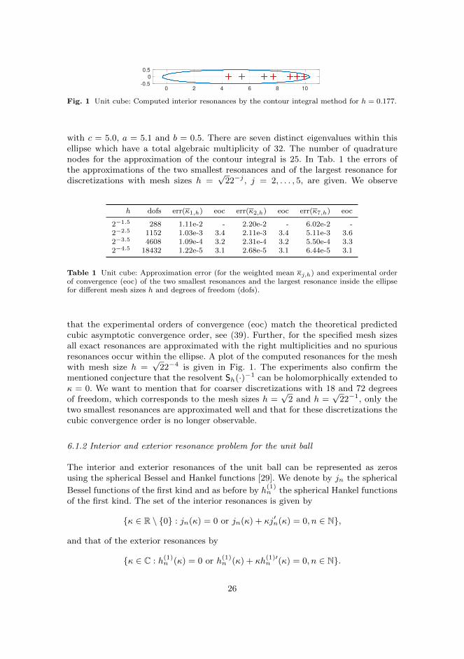
Fig. 1 Unit cube: Computed interior resonances by the contour integral method for h = 0.177.

with c = 5.0, a = 5.1 and b = 0.5. There are seven distinct eigenvalues within thisellipse which have a total algebraic multiplicity of 32. The number of quadraturenodes for the approximation of the contour integral is 25. In Tab. 1 the errors ofthe approximations of the two smallest resonances and of the largest resonance fordiscretizations with mesh sizes h =

√22−j , j = 2, . . . , 5, are given. We observe

h dofs err(κ1,h) eoc err(κ2,h) eoc err(κ7,h) eoc

2−1.5 288 1.11e-2 - 2.20e-2 - 6.02e-2 -2−2.5 1152 1.03e-3 3.4 2.11e-3 3.4 5.11e-3 3.62−3.5 4608 1.09e-4 3.2 2.31e-4 3.2 5.50e-4 3.32−4.5 18432 1.22e-5 3.1 2.68e-5 3.1 6.44e-5 3.1

Table 1 Unit cube: Approximation error (for the weighted mean κj,h) and experimental orderof convergence (eoc) of the two smallest resonances and the largest resonance inside the ellipsefor different mesh sizes h and degrees of freedom (dofs).

that the experimental orders of convergence (eoc) match the theoretical predictedcubic asymptotic convergence order, see (39). Further, for the specified mesh sizesall exact resonances are approximated with the right multiplicities and no spuriousresonances occur within the ellipse. A plot of the computed resonances for the meshwith mesh size h =

√22−4 is given in Fig. 1. The experiments also confirm the

mentioned conjecture that the resolvent Sh(·)−1 can be holomorphically extended toκ = 0. We want to mention that for coarser discretizations with 18 and 72 degreesof freedom, which corresponds to the mesh sizes h =

√2 and h =

√22−1, only the

two smallest resonances are approximated well and that for these discretizations thecubic convergence order is no longer observable.

6.1.2 Interior and exterior resonance problem for the unit ball

The interior and exterior resonances of the unit ball can be represented as zerosusing the spherical Bessel and Hankel functions [29]. We denote by jn the spherical

Bessel functions of the first kind and as before by h(1)n the spherical Hankel functions

of the first kind. The set of the interior resonances is given by

κ ∈ R \ 0 : jn(κ) = 0 or jn(κ) + κj′n(κ) = 0, n ∈ N,

and that of the exterior resonances by

κ ∈ C : h(1)n (κ) = 0 or h(1)

n (κ) + κh(1)′n (κ) = 0, n ∈ N.

26

0 2 4 6 8 10

-1

0

1

Fig. 2 Unit ball: Computed interior (plus sign) and exterior (cross) resonances by the contourintegral method for h = 0.177.

As contour for the contour integral method the ellipse ϕ(t) = c+ a cos(t) + ib sin(t),t ∈ [0, 2π], is chosen with c = 5.0, a = 5.3 and b = 1.0. There are 23 distincteigenvalues within this ellipse having a total algebraic multiplicity of 157. For theapproximation of the contour integral 100 quadrature nodes are taken. In Tab. 2the errors of the smallest and the largest interior and exterior resonance in modulusinside the ellipse are given. The experimental convergence order is in contrast to the

h dofs err(κe1,h) eoc err(κi

1,h) eoc err(κerr4,h) eoc e(κi

19,h) eoc

0.32 720 7.80e-3 - 2.15e-2 - 3.26e-2 - 7.11e-2 -0.16 2880 1.95e-3 2.0 5.37e-3 2.01 7.80e-3 2.1 1.87e-2 1.90.08 11520 4.88e-4 2.0 1.34e-3 2.00 1.91e-3 2.0 4.78e-3 2.00.04 46080 1.14e-4 2.1 3.35e-4 2.00 4.73e-4 2.0 1.21e-3 2.0

Table 2 Unit ball: Approximation error (for the weighted mean κi/ej,h) and experimental order

of convergence (eoc) of the smallest and the largest interior and exterior resonance in modulusinside the ellipse for different mesh sizes h and degrees of freedom (dofs).

cube of one order reduced since the sphere is approximated by flat triangles. Again,all exact resonances are approximated with the right multiplicities and no spuriousresonances occur. In Fig. 2 the computed resonances by the contour integral methodfor the mesh with mesh size h = 0.082 are plotted.

6.2 Scattering resonance problem for a penetrable scatterer

In this subsection we consider the Galerkin approximation of the boundary inte-gral formulation (43) of the scattering resonance problem for the penetrable scat-terer (40). The domains Ωi for the numerical examples are again the unit cube andthe unit ball. As approximation space we choose V0

h ×V0h = RT0(Th)×RT0(Th).

6.2.1 Unit cube

For this example the material parameters are set to ε1 = 4.0 and ε2 = µ1 = µ2 = 1.0.The exact resonances of the resonance problem for a penetrable cube are not known.As reference resonances the computed resonances of a very fine mesh with mesh sizeh = 0.03125 are taken. As contour for the contour integral method we chose theellipse ϕ(t) = c + a cos(t) + ib sin(t), t ∈ [0, 2π], with c = 2.5, a = 2.7 and b = 0.5.

27

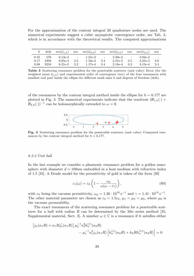
For the approximation of the contour integral 20 quadrature nodes are used. Thenumerical experiments suggest a cubic asymptotic convergence order, see Tab. 3,which is in accordance with the theoretical results. The computed approximations

h dofs err(ω1,h) eoc err(ω2,h) eoc err(ω3,h) eoc err(ω4,h) eoc

0.35 576 6.14e-3 - 1.21e-2 - 2.30e-2 - 3.94e-2 -0.17 2304 6.05e-4 3.3 1.16e-3 3.4 2.21e-3 3.5 3.25e-3 3.60.08 9216 6.21e-5 3.2 1.17e-4 3.4 2.18e-4 3.3 3.15e-4 3.4

Table 3 Scattering resonance problem for the penetrable scatterer (unit cube): Error (for theweighted mean ωj,h) and experimental order of convergence (eoc) of the four resonances withsmallest real part inside the ellipse for different mesh sizes h and degrees of freedom (dofs).

of the resonances by the contour integral method inside the ellipse for h = 0.177 areplotted in Fig. 3. The numerical experiments indicate that the resolvent (B1,h(·) +B2,h(·))−1 can be holomorphically extended to ω = 0.

0 1 2 3 4 5

-0.5

0

0.5

Fig. 3 Scattering resonance problem for the penetrable scatterer (unit cube): Computed reso-nances by the contour integral method for h = 0.177.

6.2.2 Unit ball

In the last example we consider a plasmonic resonance problem for a golden nano-sphere with diameter d = 100nm embedded in a host medium with refractive indexof 1.5 [35]. A Drude model for the permittivity of gold is taken of the form [30]

ε1(ω) = ε0

(1− ωp

ω(ω − iγ)

), (60)

with ε0 being the vacuum permittivity, ωp = 1.26 · 1016 s−1 and γ = 1.41 · 1014 s−1.The other material parameter are chosen as ε2 = 1.5ε0, µ1 = µ2 = µ0, where µ0 isthe vacuum permeability.

The exact resonances of the scattering resonance problem for a penetrable scat-terer for a ball with radius R can be determined by the Mie series method [35,Supplemental material, Sect. 3]. A number ω ∈ C is a resonance if it satisfies either[

jn(κ1R) + κ1Rj′n(κ1R)

]µ−1

2 κ22h

(1)n (κ2R)

− µ−11 κ2

1jn(κ1R)[h(1)n (κ2R) + k2Rh

(1)′n (κ2R)

]= 0

28

or

jn(κ1R)µ−12

[h(1)n (κ2R) + κ2Rh

(1)′n (κ2R)

]− h(1)

n (κ2R)µ−11

[jn(κ1R) + κ1Rj

′n(κ1R)

]= 0, (61)

for some n ∈ N, where κ` = ω√ε`(ω)µ`(ω), ` = 1, 2.

In plasmonics those scattering resonances are of interest which are close to thefrequency range of light which corresponds to [1.7, 3.1]−1, where is the reducedPlanck constant in eV·s given by = 6.58211957e-16. For the contour integralmethod as contour an ellipse is chosen with ϕ(t) = −1 [c+ a cos(t) + ib sin(t)],t ∈ [0, 2π], with c = 2.5, a = 1.4 and b = 0.75. The number of quadraturenodes for the approximation of the contour integral is 20. Three distinct resonanceswith total algebraic multiplicity of 15 lie inside the ellipse, which are solutions ofequation (61) for n = 1, 2, 3. The principal square root, with the branch cut along

h [nm] dofs r-err(ω1,h) eoc r-err(ω2,h) eoc r-err(ω3,h) eoc

35.35 288 2.88e-2 - 1.56e-2 - 9.44e-3 -16.25 1812 4.65e-3 2.34 2.50e-3 2.64 1.37e-3 2.797.67 7710 1.06e-3 1.97 5.67e-4 2.14 3.24e-3 2.083.58 33240 2.40e-4 1.95 1.35e-4 2.07 7.44e-4 2.12

Table 4 Golden ball with diameter d = 100 nm: Relative approximation error (for the weightedmean ωj,h) and experimental order of convergence (eoc) of the scattering resonances inside theellipse for different mesh sizes h and degrees of freedom (dofs).

the non-positive real axis, applied to the permittivity ε1(ω) defined in (60) is non-continuous along the contour. Instead we take the square root with the branch cutz = r(cos(φ0) + i sin(φ0)) : r ≥ 0, φ0 = 1.9π, which guarantees that

√ε1(ω)µ1

is continuous along the contour and inside of it. In Tab. 4 the relative error andthe experimental order of convergence for the approximation of the resonances in-side the contour are given. The convergence order is compared to the cube of oneorder reduced as expected since the sphere is approximated by flat triangles. Again,

1 2 3 4

-0.5

0

0.5

Fig. 4 Golden ball with diameter d = 100 nm: Computed scattering resonances by the contourintegral method for h = 7.67nm. (The axes are scaled by a factor of ).

all eigenvalues inside the ellipse are approximated with the right multiplicity and

29

no spurious eigenvalues occur. In Fig. 4 the computed resonances by the contourintegral method for the mesh with mesh size h = 7.67 are plotted.

7 Conclusions

In this paper we have analyzed the Galerkin approximation of boundary integralformulations for three different types of electromagnetic resonance problems. Wehave considered the single layer boundary integral formulation for the interior andexterior resonance problem with perfect conducting boundary conditions and a firstkind boundary integral formulation of the resonance problem for the penetrablescatterer. These boundary integral formulations are eigenvalue problems for holomor-phic Fredholm operator-valued functions. For the numerical approximation of theseeigenvalue problems a Galerkin approximation with Raviart–Thomas and Brezzi–Douglas–Marini type elements are considered. The extension of recent results [15,16] on the regular approximations of operators satisfying a generalized Garding’sinequality enables us to apply the classical convergence theory on the approxima-tion of eigenvalue problems for holomorphic Fredholm operator-valued functions tothe proposed boundary element approximations. Numerical examples confirm thetheoretical convergence results and show that the asymptotic convergence behaviorappears on rather coarse meshes.

References

1. Asakura, J., Sakurai, T., Tadano, H., Ikegami, T., Kimura, K.: A numerical method fornonlinear eigenvalue problems using contour integrals. JSIAM Letters 1, 52–55 (2009)

2. Beyn, W.J.: An integral method for solving nonlinear eigenvalue problems. Linear AlgebraAppl. 436(10), 3839–3863 (2012)

3. Bramble, J.H., Kolev, T.V., Pasciak, J.E.: The approximation of the Maxwell eigenvalueproblem using a least-squares method. Math. Comp. 74(252), 1575–1598 (electronic) (2005)

4. Buffa, A.: Remarks on the discretization of some noncoercive operator with applications toheterogeneous Maxwell equations. SIAM J. Numer. Anal. 43(1), 1–18 (electronic) (2005)

5. Buffa, A., Christiansen, S.H.: The electric field integral equation on Lipschitz screens: defi-nitions and numerical approximation. Numer. Math. 94(2), 229–267 (2003)

6. Buffa, A., Costabel, M., Schwab, C.: Boundary element methods for Maxwell’s equations onnon-smooth domains. Numer. Math. 92(4), 679–710 (2002)

7. Buffa, A., Costabel, M., Sheen, D.: On traces for H(curl, Ω) in Lipschitz domains. J. Math.Anal. Appl. 276(2), 845–867 (2002)

8. Buffa, A., Hiptmair, R.: Galerkin boundary element methods for electromagnetic scattering.In: Topics in computational wave propagation, Lect. Notes Comput. Sci. Eng., vol. 31, pp.83–124. Springer, Berlin (2003)

9. Buffa, A., Hiptmair, R., von Petersdorff, T., Schwab, C.: Boundary element methods forMaxwell transmission problems in Lipschitz domains. Numer. Math. 95(3), 459–485 (2003)

10. Christiansen, S.H.: Discrete Fredholm properties and convergence estimates for the electricfield integral equation. Math. Comp. 73(245), 143–167 (2004)

11. Colton, D., Kress, R.: Inverse acoustic and electromagnetic scattering theory, Applied Math-ematical Sciences, vol. 93, third edn. Springer, New York (2013)

12. Cossonniere, A.: Valeurs propres de transmission et leur utilisation dans l’identificationd’inclusions a partir de mesures electromagnetiques. Phd thesis, INSA Toulouse (2011)

13. Duran, M., Nedelec, J.C., Ossandon, S.: An efficient Galerkin BEM to compute high acousticeigenfrequencies. J. Vib. Acoust. 131(3), (31001)1–9 (2009)

30

14. Gohberg, I., Goldberg, S., Kaashoek, M.A.: Classes of Linear Operators. Vol. I. BirkhauserVerlag, Basel (1990)

15. Halla, M.: Analysis of radial complex scaling methods for scalar resonance problems in opensystems. Ph.d. thesis, TU Vienna (2019)

16. Halla, M.: Galerkin approximation of holomorphic eigenvalue problems: weak T-coercivityand T-compatibility. arXiv e-prints arXiv:1908.05029 (2019)

17. Karma, O.: Approximation in eigenvalue problems for holomorphic Fredholm operator func-tions. I. Numer. Funct. Anal. Optim. 17(3-4), 365–387 (1996)

18. Karma, O.: Approximation in eigenvalue problems for holomorphic Fredholm operator func-tions. II. (Convergence rate). Numer. Funct. Anal. Optim. 17(3-4), 389–408 (1996)

19. Kato, T.: Perturbation Theory for Linear Operators. Classics in Mathematics. Springer-Verlag, Berlin (1995)

20. Kimeswenger, A., Steinbach, O., Unger, G.:21. Kirsch, A., Hettlich, F.: The mathematical theory of time-harmonic Maxwell’s equations,

Applied Mathematical Sciences, vol. 190. Springer, Cham (2015)22. Kleefeld, A.: Numerical methods for acoustic and electromagnetic scattering: Transmission

boundary-value problems, interior transmission eigenvalues, and the factorization method.Habilitation thesis, BTU Cottbus-Senftenberg (2015)

23. Kozlov, V., Maz′ya, V.: Differential Equations with Operator Coefficients with Applicationsto Boundary Value Problems for Partial Differential Equations. Springer Monographs inMathematics. Springer-Verlag, Berlin (1999)

24. Maakitalo, J., Kauranen, M., Suuriniemi, S.: Modes and resonances of plasmonic scatterers.Phys. Rev. B 89, 165429 (2014)

25. McLean, W.: Strongly Elliptic Systems and Boundary Integral Equations. Cambridge Uni-versity Press, Cambridge (2000)

26. Misawa, R., Niino, K., Nishimura, N.: Boundary integral equations for calculating complexeigenvalues of transmission problems. SIAM Journal on Applied Mathematics 77(2), 770–788(2017)

27. Monk, P.: Finite element methods for Maxwell’s equations. Oxford University Press, NewYork (2003)

28. Nannen, L., Hohage, T., Schadle, A., Schoberl, J.: Exact sequences of high order Hardy spaceinfinite elements for exterior Maxwell problems. SIAM J. Sci. Comput. 35(2), A1024–A1048(2013)

29. Nedelec, J.C.: Acoustic and electromagnetic equations. Springer-Verlag, New York (2001)30. Sauvan, C., Hugonin, J.P., Maksymov, I.S., Lalanne, P.: Theory of the spontaneous optical

emission of nanosize photonic and plasmon resonators. Phys. Rev. Lett. 110, 237401 (2013)

31. Smigaj, W., Arridge, S., Betcke, T., Phillips, J., Schweiger, J.: Solving Boundary IntegralProblems with BEM++. ACM Trans. Math. Software 41(6), 1–40 (2015)

32. Steinbach, O.: Numerical Approximation Methods for Elliptic Boundary Value Problems.Finite and Boundary Elements. Springer, New York (2008)

33. Steinbach, O., Unger, G.: Convergence analysis of a Galerkin boundary element method forthe Dirichlet Laplacian eigenvalue problem. SIAM J. Numer. Anal. 50, 710–728 (2012)

34. Steinbach, O., Unger, G.: Combined boundary integral equations for acoustic scattering-resonance problems. Math. Methods Appl. Sci. 40(5), 1516–1530 (2017)

35. Unger, G., Trugler, A., Hohenester, U.: Novel modal approximation scheme for plasmonictransmission problems. Phys. Rev. Lett. 121, 246802 (2018)

36. Vainikko, G.: Approximative methods for nonlinear equations (two approaches to the con-vergence problem). Nonlinear Anal. 2(6), 647–687 (1978)

37. Wieners, C., Xin, J.: Boundary element approximation for Maxwell’s eigenvalue problem.Math. Methods Appl. Sci. 36(18), 2524–2539 (2013)

38. Yokota, S., Sakurai, T.: A projection method for nonlinear eigenvalue problems using contourintegrals. JSIAM Lett. 5, 41–44 (2013)

31