CONVENTIONAL AND UNCONVENTIONAL MONETARY POLICY … · Conventional monetary policy (interest-rate...
30
CONVENTIONAL AND UNCONVENTIONAL MONETARY POLICY WITH ENDOGENOUS COLLATERAL CONSTRAINTS ALO ´ ISIO ARA ´ UJO, SUSAN SCHOMMER, AND MICHAEL WOODFORD Abstract. In this paper we consider a finite horizon model with default and monetary policy. In our model, each asset promises delivery of either one unit of money in the next period or of a real collateral payoff in case of default. Moreover, we include the possibility of purchases of the collateralizable durable good by the central bank. This is done in order to add an additional dimension of monetary policy, which may be of particular relevance when the interest rate reaches the zero lower bound (as has happened in the recent financial crisis). In order to implement such a policy, we must additionally include a rental market for the durable good (so that durables purchased by the central bank can still be used by agents). We examine through numerical examples how the purchases of the central bank affect the equilibrium allocations of resources, and under which conditions such a policy can lead to a Pareto-improvement. Date : April 7, 2011. 1
Transcript of CONVENTIONAL AND UNCONVENTIONAL MONETARY POLICY … · Conventional monetary policy (interest-rate...
CONVENTIONAL AND UNCONVENTIONAL MONETARY POLICYWITH ENDOGENOUS COLLATERAL CONSTRAINTS
ALOISIO ARAUJO, SUSAN SCHOMMER, AND MICHAEL WOODFORD
Abstract. In this paper we consider a finite horizon model with default and monetary
policy. In our model, each asset promises delivery of either one unit of money in the next
period or of a real collateral payoff in case of default. Moreover, we include the possibility
of purchases of the collateralizable durable good by the central bank. This is done in order
to add an additional dimension of monetary policy, which may be of particular relevance
when the interest rate reaches the zero lower bound (as has happened in the recent financial
crisis). In order to implement such a policy, we must additionally include a rental market
for the durable good (so that durables purchased by the central bank can still be used by
agents).
We examine through numerical examples how the purchases of the central bank affect
the equilibrium allocations of resources, and under which conditions such a policy can lead
to a Pareto-improvement.
Date: April 7, 2011.
1
2 ALOISIO ARAUJO, SUSAN SCHOMMER, AND MICHAEL WOODFORD
1. Introduction
In response to the recent financial crisis, central banks cut interest rates sharply, and
in some cases (as with the U.S. Federal Reserve) essentially to the lower bound of a zero
nominal rate. The inability to use conventional interest-rate policy more aggressively, under
circumstances of low real activity and declining inflation, led many central banks to resort to
“unconventional” policies, involving purchases of assets by the central bank, or extensions of
credit to private institutions, beyond those required to implement the central bank’s target
for the short-term nominal interest rate [CWo].
In this paper, we extend a general equilibrium model with collateral (GEIC) of the kind
developed by [GZ] to include money and purchases of a durable good by the central bank.
In our model, each asset promises delivery of one unit of money in the next period and a
real collateral payoff in case of default. Each agent begins with an initial endowment of
money, and additional money can be issued by the central bank to finance asset purchases.
Conventional monetary policy (interest-rate policy) is introduced by allowing the central
bank to specify the nominal interest rate on its liabilities: one unit of money held today
becomes a claim to a certain number of units of money tomorrow, regardless of the states
of nature.1 Because we work for simplicity with a finite-horizon model, the value of money
in the final period is determined by redemption of the outstanding money stock for goods
1In actual economies, the central bank’s policy rate is distinct from the interest rate paid on reserve
balances at the central bank (the “money” in our model), and the central bank influences the value of that
policy rate both by varying the interest rate paid on reserves and by varying the differential between the two
interest rates through variation in the supply of reserves. The latter aspect of policy (typically emphasized
in textbook discussions of monetary policy) depends on a reason for reserves to be valued more than other
assets paying the same pecuniary return in each state; for simplicity, we abstract from such non-pecuniary
returns to money here, and allow interest-rate policy to be implemented purely through variations in the
rate of interest paid on money, as in the “cashless” model proposed in [Wo] chapter 2. For an example of
a model in which the policy rate can also be influenced by varying the supply of reserves, see for example
[CWo].
MONETARY POLICY WITH ENDOGENOUS COLLATERAL CONSTRAINTS 3
by the central bank; the revenue required to redeem the money supply is raised through
lump-sum taxation.
In this model, we also consider the possibility of purchases of the durable good by central
bank, paid for by issuance of money. In the recent crisis, the market value of the most
important collateralizable durable good (real estate) fell significantly, resulting in increased
defaults by debtors and significant losses for financial institutions. Declines in the market
value of other types of collateral (financial claims used as collateral for new borrowing by
financial institutions) also played an important role in the crisis, and one possible goal of
“unconventional” policy might be to raise the market value of such collateral. (In practice,
such policies were addressed more to the value of collateralizable financial claims, but in our
model the only form of collateral is a real durable good, and so we consider the possibility
of affecting the equilibrium value of that good.) In fact, it is not obvious that central-bank
purchases must change equilibrium asset prices; [Wa] presents a general-equilibrium analysis
in which open-market purchases by the central bank have no effect on equilibrium asset
prices or on the allocation of resources. As [CWo] discuss further, in a GEI model without
collateral constraints, both the size and composition of the central-bank balance sheet are
irrelevant, though the existence of additional financial constraints can break the irrelevance
result. In our model, the existence of the collateral constraint breaks the irrelevance result,
and we find in most cases that central-bank purchases do affect the equilibrium price of the
durable good.
In section 2, we first present a two-period flexible price model and show that in the
“cashless limit” of this model (when money balances are negligible), variations in interest-
rate policy have no effect on the equilibrium allocation of resources. With sticky prices (our
second model), instead, interest-rate policy affects the equilibrium allocation, even in the
cashless limit. In this second model, there is an arbitrarily given predetermined price level
for the non-durable good in the initial period; but it may not be realistic to suppose that we
can choose any monetary policy we like without the anticipation of that policy having had
4 ALOISIO ARAUJO, SUSAN SCHOMMER, AND MICHAEL WOODFORD
an effect on the way that prices were set. Hence we consider a third model, in which the
non-durable good price and supply commitments are endogenized (modeled as being chosen
before agents learn the period 0 state of the world). Here we consider different possible states
in the first period, but assume that the values of non-durable price and supply commitments
are chosen prior to the realization of the state, and so are the same for all states in the
first period. We examine through numerical examples how the welfare-maximizing choice of
interest-rate policy (in each state in the first period) is different depending on the severity of
collateral constraints. We present an example in which in the bad state (in which collateral
constraints are binding) the optimal nominal interest rate is zero, so that the interest-rate
lower bound is a binding constraint. This makes the question of the efficacy of alternative
dimensions of policy particularly interesting.
In section 3, we consider the effects of purchases of the collateralizable durable good by
the central bank in the two-period flexible-price model. We show that when markets are
endogenously incomplete and collateral constraints are binding, this additional dimension of
monetary policy affects equilibrium asset prices. We then consider the welfare effects of the
use of this kind of policy, in some simple numerical examples involving two types of agents
(rich and poor). In the numerical examples presented in section 4, we generally find that the
poor agent gains from purchases of durable good by the central bank, while the rich agent
loses; thus the policy is not irrelevant, but cannot achieve a Pareto improvement. We also
find that the distribution of taxes and transfers (and hence the distribution of net central-
bank earnings from trading), and in particular the way that this depends on the states of
nature, is quite important for the equilibrium effects of the central-bank purchases. When
the distribution of taxes is the same across states, central-bank purchases of the durable good
can lead to Pareto-improvements, given that the utility of the rich agent is little affected,
while it is possible to improve the utility of the poor agent to a significant extent through
purchases of the durable in the bad state where the zero lower bound constrains interest-rate
policy.
MONETARY POLICY WITH ENDOGENOUS COLLATERAL CONSTRAINTS 5
2. A two period model with one dimension of monetary policy
We first consider a two period model, which includes money in a general equilibrium
model with collateral. In this model, we examine the effect of the monetary policy, through
interest rate. We show that in the cashless limit (money supply goes to zero), variations in
interest rate policy have no effect on the equilibrium. If we consider that prices are sticky,
interest-rate policy effects the equilibrium allocation of resources, even in the cashless limit.
2.1. Basic monetary model: flexible prices. We consider a pure exchange economy over
two time periods t = 0, 1 with uncertainty over the state of nature in period 1 denoted by
the subscript s ∈ S = {1, . . . , S}.
The economy consists of a finite number H of agents denoted by the superscript h ∈
H = {1, . . . H} and L = 2 goods or commodities, denoted by the subscript l ∈ L = {1, 2}.
Throughout the analysis we assume that good 1 is perishable and good 2 is durable, i.e. there
is a possibly risky (and possibly productive) storage technologies, represented by Ys ∈ R2+.
Using one unit of the durable good in the first period yields Ysl units of good l in state s.
The most natural assumption is of course that Ys = (0, 1) for each state s, i.e. it is possible
to store the durable good without depreciation. Each agent has an initial endowment of the
goods in each state, eh ∈ R2(S+1)+ . The preference ordering of agent h is represented by a
utility function uh : R2(S+1)+ → R, defined over consumption xh = (xh, xh1 , . . . , x
hS) ∈ R2(S+1)
+ .
Money: each agent h has an endowment of money in the amount mh in period 0, where∑hm
h = M > 0 is the money supply. Monetary policy also specifies the nominal interest
rate i: one unit of money hold in period 0 becomes a claim to (1 + i) units of money in
period 1, regardless of the states s. Finally, monetary policy specifies the redemption value of
money in each state s in period 1. Each unit of money is redeemed for a specified (positive)
number of units of good 1 in state s; then for each state s, the price ps1 of good 1 in units
of money is fixed by monetary policy. The revenues required to redeem the money supply
are raised through lump-sum taxation. The share of taxes raised from each household h in
6 ALOISIO ARAUJO, SUSAN SCHOMMER, AND MICHAEL WOODFORD
state s is θhs ≥ 0, where∑
h θhs = 1 for each state s. Hence the tax obligation of household
h in state s (in units of good 1) is θhsM(1 + i)/ps1; or θhsM(1 + i) in units of money.
The fact that the money is redeemed for goods in the terminal period is a way of rep-
resenting the fact that in an actual economy (with a terminal period), the value of money
each period is determined by monetary policy (in that period and later). Since there is no
interest rate in the terminal period, and no value of end-of-period money balances, the only
way that monetary policy can determine the price level in this period is by specifying the
redemption value of money, as under a commodity money regime.
Additional assets: each asset j promises delivery of one unit of money in period 1,
regardless of the state s. The collateral requirements for asset j is Cj ≥ 0; any agent has to
hold Cj units of good 2 in period 0 in order to sell 1 unit of asset j. Given the possibility of
default the actual payoff of asset j in state s is min(1, ps2Cj) in units of money, here ps2 is
the spot price of good 2 (in units of money) in state s, period 1.
Given p ∈ R2(S+1)++ , and q ∈ RJ
+ the agent h chooses consumption, portfolios and money
(xh, ψh, ϕh, µh), to maximize utility subject to the budget constraints.
maxx≥0,ψ≥0,ϕ≥0,µ≥0
uh(xh) s.t.
p · (xh − eh) + q · (ψ − ϕ) + µh −mh ≤ 0;
ps · (xhs − ehs )− ps2xh2 −∑j∈J
(ψhj − ϕhj ) min{1, ps2Cj}+ (1 + i)(θhsM − µh) ≤ 0; ∀s ∈ S
xh2 −∑j∈J
ϕhjCj ≥ 0.
(2.1)
A competitive equilibrium is defined as usual by agents’ optimality and market clearing.
Definition 1. An equilibrium for the economy E is a vector [(x, ψ, ϕ, µ); (p, q)], such that:
(i) (xh, ψh, ϕh, µh) solves problem 2.1.
MONETARY POLICY WITH ENDOGENOUS COLLATERAL CONSTRAINTS 7
(ii)∑H
h=1(xh − eh) = 0
(iii)∑H
h=1(xhs1 − ehs1) = 0 and
∑Hh=1(x
hs2 − ehs2 − xh2) = 0, s = 1, . . . , S
(iv)∑H
h=1(ψh − ϕh) = 0
(v)∑H
h=1 µh −M = 0
In this model changes in the quantities of money, or interest rate or taxation will have
effects on equilibrium, but if we consider the limiting case in which M → 0 we show that
money is neutral.
“Cashless limit”: The analysis is simplified if we consider the limiting case in which
M → 0, so that we can abstract from redistributive effects of changes in the nominal price
level. In this case, monetary policy is simply specified by 1 + i > 0 and the {ps1}. The
initial endowments mh are also set to zero, and the specification of the tax shares {θhs} no
longer matters. In this case, the economy is completely characterized by the agents’ utility
functions {uh}, their endowments {eh}, the asset structure {Cj}, and the monetary policy
(i, {ps1}). The following proposition shows that monetary policy is neutral in the cashless
limit.
Proposition 1. Neutrality of money: In the flexible-price model, with cashless limit
[M → 0, and mh → 0 ∀h as a convergence], variations in interest-rate policy have no
effect on the equilibrium allocation of resources.
Proof. the household by problem, and hence all equilibrium conditions, can be written
entirely in terms of quantitiesµ
p1,p2p1,q
p1, and(1 + i)p1, with no reference to p1 or i individ-
ually. Hence the real allocation x, the portfolios, and relative prices are all determined by
data that do not involve i. It follows that changing i changes the value of p1, so as to keep
(1 + i)p1, the same, but has no effect in the real allocation or on relative prices. �
Central-bank balance sheet: It may be more realistic to suppose that the money
supply M represents liabilities of a central bank, which has corresponding assets on its
balance sheet. [This is of interest if one wishes to consider the effects of alternative kinds of
8 ALOISIO ARAUJO, SUSAN SCHOMMER, AND MICHAEL WOODFORD
asset purchases by the central bank.] The above model can be equivalent desenhed as one
in which the central bank holds riskless government debt as an asset, of the same value as
its liabilities M . In equilibrium, the riskless government debt must earn the same interest
rate i as the liabilities of the central bank, so the central bank has no income or losses in
period 1. The taxes in period 1 can now be thought of as being levied in order to pay off
the government debt in period 1. Later, we generalize the model to allow the central bank
to hold other assets as well. In this case, the central bank can have income or losses on its
portfolio, which are distributed to the Treasury, and so affect the state-contingent taxes that
must be collected from the agents.
2.1.1. Example: Cashless limit in the flexible price model. We consider a simple example
with two states in period 1 S = 2, two agents H = 2 and two assets J = 2. Each individual
h = has a utility function of the form:
uh(x) = log(x1) + log(x2) +1
2
2∑s=1
(log(xs1) + log(xs2))
Endowments are:
e1 = (e11, e12, e
111, e
112, e
121, e
122) = (4, 1, 4, 0, 4, 0);
e2 = (e21, e22, e
211, e
212, e
221, e
222) = (2, 1, 6, 0, 2, 0).
To illustrate the cashless limit in the flexible price model, we consider several quantity of
money supply in which M → 0 M = [1; 0.8; 0.5; 0.1; 0.001].
Money mh in the first period are: m1 = 0.7 ∗M ; m2 = 0.3 ∗M .
Taxes θhs are: θ1 = (θ11, θ12) = (0.5, 0.5); θ2 = (θ21, θ
22) = (0.5, 0.5).
In the second period the price of non-durable good ps1 is fixed: p11 = 1; p21 = 1.
The collateral requirements are: C1 = 0.2; C2 = 0.333.
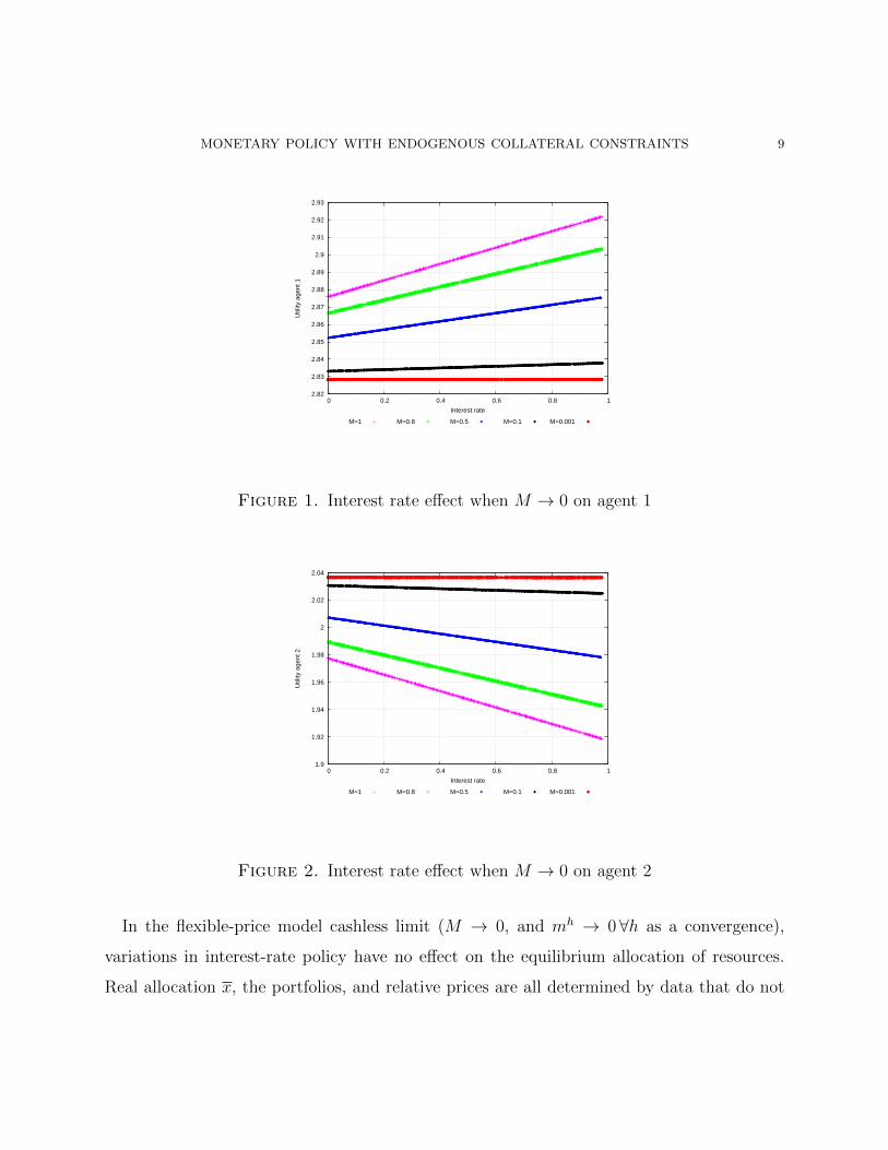
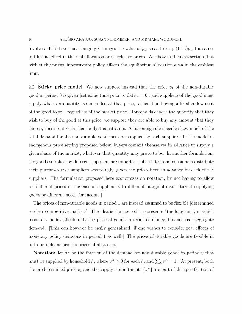
In the Figures 1 and 2, we show a few different points in utility space with random choice
of the interest rate between 0 and 1.
MONETARY POLICY WITH ENDOGENOUS COLLATERAL CONSTRAINTS 9
2.82
2.83
2.84
2.85
2.86
2.87
2.88
2.89
2.9
2.91
2.92
2.93
0 0.2 0.4 0.6 0.8 1
Util
ity a
gent
1
Interest rate
M=1 M=0.8 M=0.5 M=0.1 M=0.001
Figure 1. Interest rate effect when M → 0 on agent 1
1.9
1.92
1.94
1.96
1.98
2
2.02
2.04
0 0.2 0.4 0.6 0.8 1
Util
ity a
gent
2
Interest rate
M=1 M=0.8 M=0.5 M=0.1 M=0.001
Figure 2. Interest rate effect when M → 0 on agent 2
In the flexible-price model cashless limit (M → 0, and mh → 0 ∀h as a convergence),
variations in interest-rate policy have no effect on the equilibrium allocation of resources.
Real allocation x, the portfolios, and relative prices are all determined by data that do not
10 ALOISIO ARAUJO, SUSAN SCHOMMER, AND MICHAEL WOODFORD
involve i. It follows that changing i changes the value of p1, so as to keep (1+ i)p1, the same,
but has no effect in the real allocation or on relative prices. We show in the next section that
with sticky prices, interest-rate policy affects the equilibrium allocation even in the cashless
limit.
2.2. Sticky price model. We now suppose instead that the price p1 of the non-durable
good in period 0 is given [set some time prior to date t = 0], and suppliers of the good must
supply whatever quantity is demanded at that price, rather than having a fixed endowment
of the good to sell, regardless of the market price. Households choose the quantity that they
wish to buy of the good at this price; we suppose they are able to buy any amount that they
choose, consistent with their budget constraints. A rationing rule specifies how much of the
total demand for the non-durable good must be supplied by each supplier. [In the model of
endogenous price setting proposed below, buyers commit themselves in advance to supply a
given share of the market, whatever that quantity may prove to be. In another formulation,
the goods supplied by different suppliers are imperfect substitutes, and consumers distribute
their purchases over suppliers accordingly, given the prices fixed in advance by each of the
suppliers. The formulation proposed here economizes on notation, by not having to allow
for different prices in the case of suppliers with different marginal disutilities of supplying
goods or different needs for income.]
The prices of non-durable goods in period 1 are instead assumed to be flexible [determined
to clear competitive markets]. The idea is that period 1 represents “the long run”, in which
monetary policy affects only the price of goods in terms of money, but not real aggregate
demand. [This can however be easily generalized, if one wishes to consider real effects of
monetary policy decisions in period 1 as well.] The prices of durable goods are flexible in
both periods, as are the prices of all assets.
Notation: let σh be the fraction of the demand for non-durable goods in period 0 that
must be supplied by household h, where σh ≥ 0 for each h, and∑
h σh = 1. [At present, both
the predetermined price p1 and the supply commitments {σh} are part of the specification of
MONETARY POLICY WITH ENDOGENOUS COLLATERAL CONSTRAINTS 11
the model. Below, we consider a more elaborate model in which they are endogenized.] Each
household has an endowment (non-negative) of each of the other 2S + 1 goods, as before.
Preferences of household h are defined by a utility function uh(xh)− vh(yh), where yh ≥ 0 is
the quantity of the non-durable good that is supplied by household h in period 0. [Additive
separability is not essential, but allows us to write the consumer demand problem in terms
of the same preferences as before.]
Given p ∈ R2(S+1)++ , q ∈ RJ
+ and aggregate demand y ∈ R+ for the non-durable good in
period 0 the agent h chooses consumption, portfolios and money (xh, ψh, ϕh, µh), to maximize
utility subject to the budget constraints.
maxx≥0,ψ≥0,ϕ≥0,µ≥0
uh(xh) s.t.
p1(xh1 − σhy) + p2(x
h2 − eh2) + qj · (ψ − ϕ) + µh −mh ≤ 0;
ps · (xhs − ehs )− ps2xh2 −∑j∈J
(ψhj − ϕhj ) min{1, ps2Cj}+ (1 + i)(θhsM − µh) ≤ 0; ∀s ∈ S
xh2 −∑j∈J
ϕhjCj ≥ 0.
(2.2)
A competitive equilibrium is defined as usual by agents’ optimality and market clearing.
Definition 2. An equilibrium for the economy E is a vector
[(x, ψ, ϕ, µ); (p, q); y] where p1 is the given (predetermined) price, that is part of the data
delivery the economy, such that:
(i) (xh, ψh, ϕh, µh) solves problem 2.2.
(ii)∑H
h=1 xh1 − y = 0
(iii)∑H
h=1(xh2 − eh2) = 0
(iv)∑H
h=1(xhs1 − ehs1) = 0 and
∑Hh=1(x
hs2 − ehs2 − xh2) = 0, s = 1, . . . , S
(v)∑H
h=1(ψh − ϕh) = 0
12 ALOISIO ARAUJO, SUSAN SCHOMMER, AND MICHAEL WOODFORD
(vi)∑H
h=1 µh −M = 0
Since p1 is predetermined, and ps1 is specified for each s by monetary policy, only p2 is
endogenously determined to satisfy the above requirements.
Under the assumption of additive separability made here, the functions vh(yh) are irrele-
vant to equilibrium determination. However, they matter for welfare evaluation of alternative
monetary policies. [They also matter for the endogenization of the predetermined price level,
treated below.]
As shown in Proposition 1, interest-rate policy has real effects in the flexible-price model
only to the extent that it changes the distribution across households of real cash balancesmh
p1(0)or of tax obligations θh(s)M(1+ i). The latter effects are not obviously of quantitative
relevance in actual economies; hence the usefulness of considering the cashless limit. With
sticky prices, instead, interest-rate policy effects the equilibrium allocation of resources even
in the cashless limit.
2.2.1. Example: Cashless limit of the sticky price model. We consider a similar economy as
in the example of section (2.1.1), but with the following modifications. Each individual h
has a utility function of the form:
Γh = uh(x)− vh(σhy)
where uh(x) has the same logarithmic form as to Example 1; and vh(σhy) = (σhy)η, with
η = 1. Endowments are:
e1 = (e12, e111, e
112, e
121, e
122) = (1, 4, 0, 4, 0);
e2 = (e22, e211, e
212, e
221, e
222) = (1, 6, 0, 2, 0).
Rationing rule for the supply of non-durable goods in period 0: σ1 = 0.67 and σ2 = 0.33.
Finally, the price of non-durable good in period 0 is given by p1 = 1.
MONETARY POLICY WITH ENDOGENOUS COLLATERAL CONSTRAINTS 13
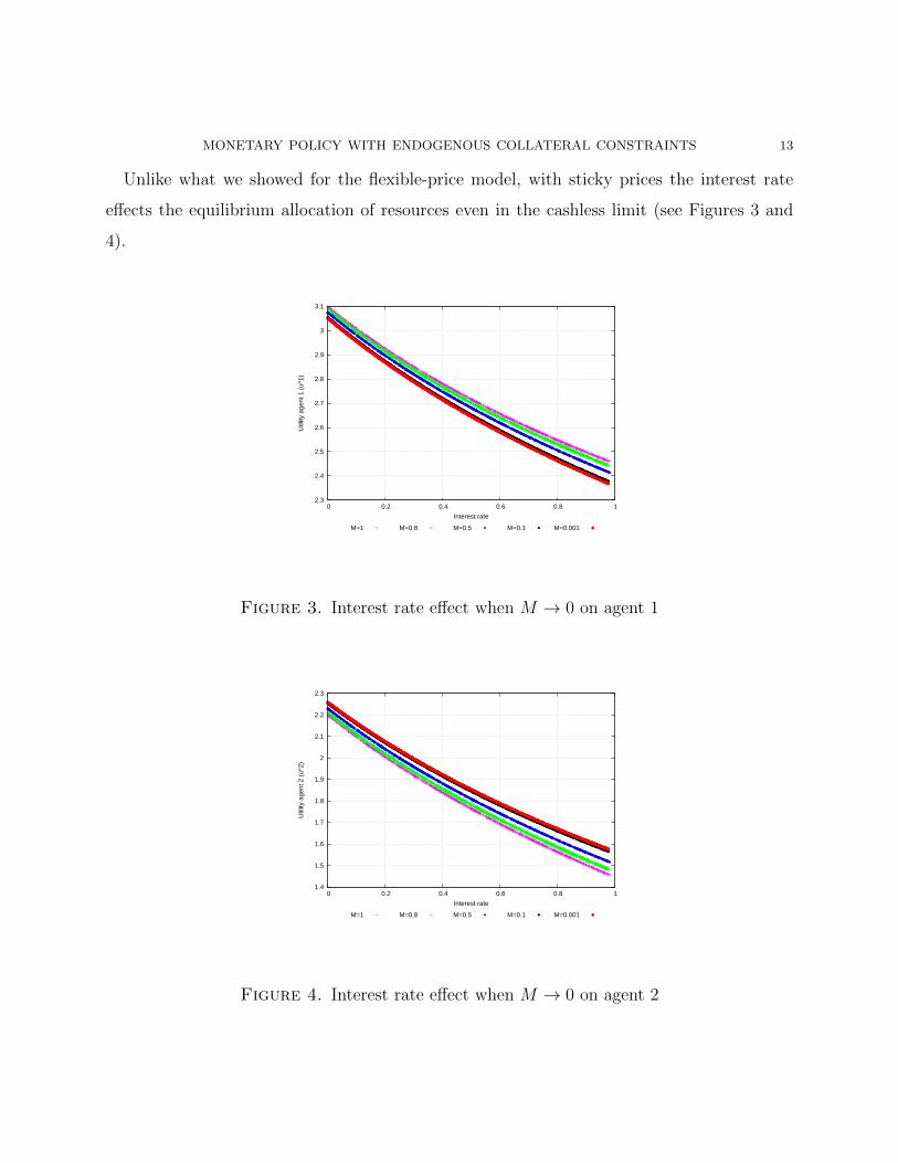
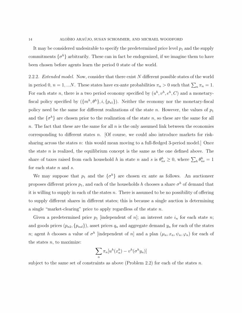
Unlike what we showed for the flexible-price model, with sticky prices the interest rate
effects the equilibrium allocation of resources even in the cashless limit (see Figures 3 and
4).
2.3
2.4
2.5
2.6
2.7
2.8
2.9
3
3.1
0 0.2 0.4 0.6 0.8 1
Util
ity a
gent
1 (
u^1)
Interest rate
M=1 M=0.8 M=0.5 M=0.1 M=0.001
Figure 3. Interest rate effect when M → 0 on agent 1
1.4
1.5
1.6
1.7
1.8
1.9
2
2.1
2.2
2.3
0 0.2 0.4 0.6 0.8 1
Util
ity a
gent
2 (
u^2)
Interest rate
M=1 M=0.8 M=0.5 M=0.1 M=0.001
Figure 4. Interest rate effect when M → 0 on agent 2
14 ALOISIO ARAUJO, SUSAN SCHOMMER, AND MICHAEL WOODFORD
It may be considered undesirable to specify the predetermined price level p1 and the supply
commitments {σh} arbitrarily. These can in fact be endogenized, if we imagine them to have
been chosen before agents learn the period 0 state of the world.
2.2.2. Extended model. Now, consider that there exist N different possible states of the world
in period 0, n = 1, ...N . These states have ex-ante probabilities πn > 0 such that∑
n πn = 1.
For each state n, there is a two period economy specified by (uh, vh, eh, C) and a monetary-
fiscal policy specified by ({mh, θh}, i, {ps1}). Neither the economy nor the monetary-fiscal
policy need be the same for different realizations of the state n. However, the values of p1
and the {σh} are chosen prior to the realization of the state n, so these are the same for all
n. The fact that these are the same for all n is the only assumed link between the economies
corresponding to different states n. [Of course, we could also introduce markets for risk-
sharing across the states n: this would mean moving to a full-fledged 3-period model.] Once
the state n is realized, the equilibrium concept is the same as the one defined above. The
share of taxes raised from each household h in state n and s is θhns ≥ 0, where∑
h θhns = 1
for each state n and s.
We may suppose that p1 and the {σh} are chosen ex ante as follows. An auctioneer
proposes different prices p1, and each of the households h chooses a share σh of demand that
it is willing to supply in each of the states n. There is assumed to be no possibility of offering
to supply different shares in different states; this is because a single auction is determining
a single “market-clearing” price to apply regardless of the state n.
Given a predetermined price p1 [independent of n]; an interest rate in for each state n;
and goods prices (pn2, {pnsl}), asset prices qn and aggregate demand yn for each of the states
n; agent h chooses a value of σh [independent of n] and a plan (µn, xn, ψn, ϕn) for each of
the states n, to maximize: ∑n
πn[uh(xhn)− vh(σhyn)]
subject to the same set of constraints as above (Problem 2.2) for each of the states n.
MONETARY POLICY WITH ENDOGENOUS COLLATERAL CONSTRAINTS 15
Definition 3. An equilibrium for the economy E is a vector (p1, σ) and vectors
[(xn, ψn, ϕn, µn); (pn, qn); yn] for each of the states n, such that:
(i) for each h, σh and (xhn, ψh
n, ϕhn, µ
hn) solves problem of individual h;
(ii) market-clearing conditions (ii)-(vi) above (Definition 2) are satisfied for each n;
(iii)∑H
h=1 σh − 1 = 0
Note that in the special case that N = 1, this concept of equilibrium reduces to the
flexible-price monetary equilibrium. It differs from the equilibrium definition above only
in that there is now an endogenous supply of the non-durable good by each household in
period 0, rather than a fixed endowment. [The case of a fixed endowment would of course
be recovered as a limiting case of this model.] Thus when N = 1, variations in interest-rate
policy have no effect in the equilibrium allocation of resources, as shown above.
What can be asked in this model: Suppose that the degree of collateral available is
different in different states n. One can then consider the consequences of specifying monetary
policy (for example, the value of in) to be different in different states n as well. In this
analysis, the state-contingent character of monetary policy will be anticipated by households
in choosing their supply commitments, and so in the determination of the predetermined
price p1. Because monetary policy is anticipated when p1 is determined if N = 1 the
specification of i has no effect on the real equilibrium allocation (only on the value of p1).
But if there are multiple possibilities (N > 1), then in general the specification of state-
contingent interest-rate policy does matter. We wish to address the following question: How
is the welfare-maximizing choice of {in} different depending what one assumes about the
severity of the collateral constraints? One can fix preferences {uh, vh} and the endowments
{eh} of the 2S + 1 goods other than the non-durable good in period 0 [for each state n], but
consider the effects of varying the collateral requirements {Cj}.
2.2.3. Example: Interest rate policy in the extended model. We consider an example with
two states in period 0, N = 2; two states in period 1, S = 2; and two agents, H = {1, 2}.
16 ALOISIO ARAUJO, SUSAN SCHOMMER, AND MICHAEL WOODFORD
Each individual h has a utility function of the form as example above in the section (2.2.1)
for each of the states n.
Ex ante probabilities are: π1 = 0.6; and π2 = 0.4.
Endowments are:
e11 = (0.1), e12 = (1.8), for l=2 e111l = (2, 0), e112l = (5, 0), e121l = (3, 0), e122l = (6, 0);
e21 = (0.9), e22 = (0.2), for l=2 e211l = (5, 0), e212l = (3, 0), e221l = (7, 0), e222l = (3, 0).
Money mhn in the first period are:
m11 = 0.5, m1
2 = 0.6;
m21 = 0.5, m2
2 = 0.4.
Money supply: M1 = 1 and M2 = 1.
Tax θhns is:
θ1 = (θ111, θ112, θ
121, θ
122) = (0.52, 0.50, 0.70, 0.45);
θ2 = (θ211, θ212, θ
221, θ
222) = (0.48, 0.50, 0.30, 0.55).
The price is fixed pns1 = 1 ∀n, ∀s.
There are four assets, J = 4.
In this example we consider that all agents have identical homothetic utility, then prices
in the period 1 do not change. According to [AKS] (Proposition 2) the level of collateral
requirements defined by Cj = 1/p(s)2 the markets chooses the asset structure efficiently. In
our case the level de collateral requirements is defined by Cj = 1/pn(s)2, where C1 = 0.143,
C2 = 0.125, C3 = 0.2 and C4 = 0.222 in this example.
We solved several samples with random choice of the nominal interest rate (i1 and i2)
between 0 and 1.
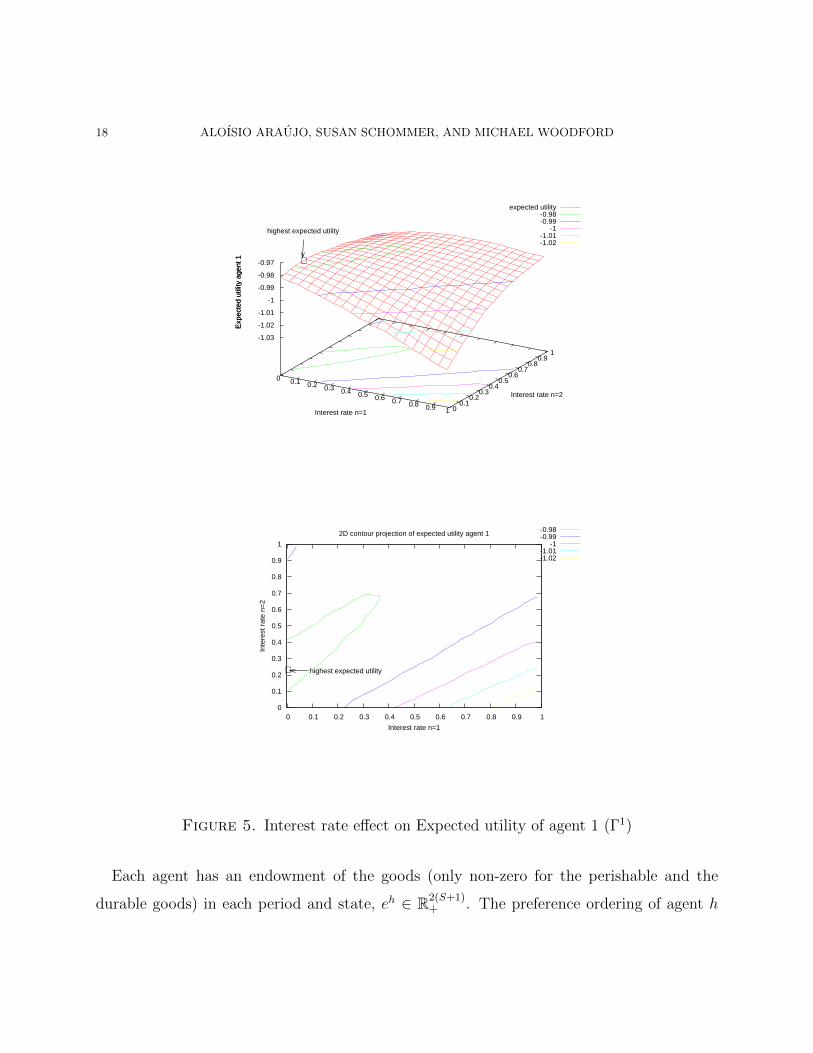
The interest-rate policy that maximizes utility for agent 1 is i1 = 0 and i2 = 0.23 (see
Figure 10), while the policy best for agent 2 is i1 = 0 and i2 = 0.16 (see Figure 11). The plot
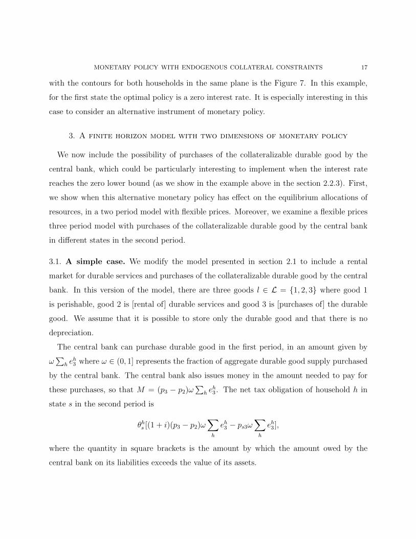
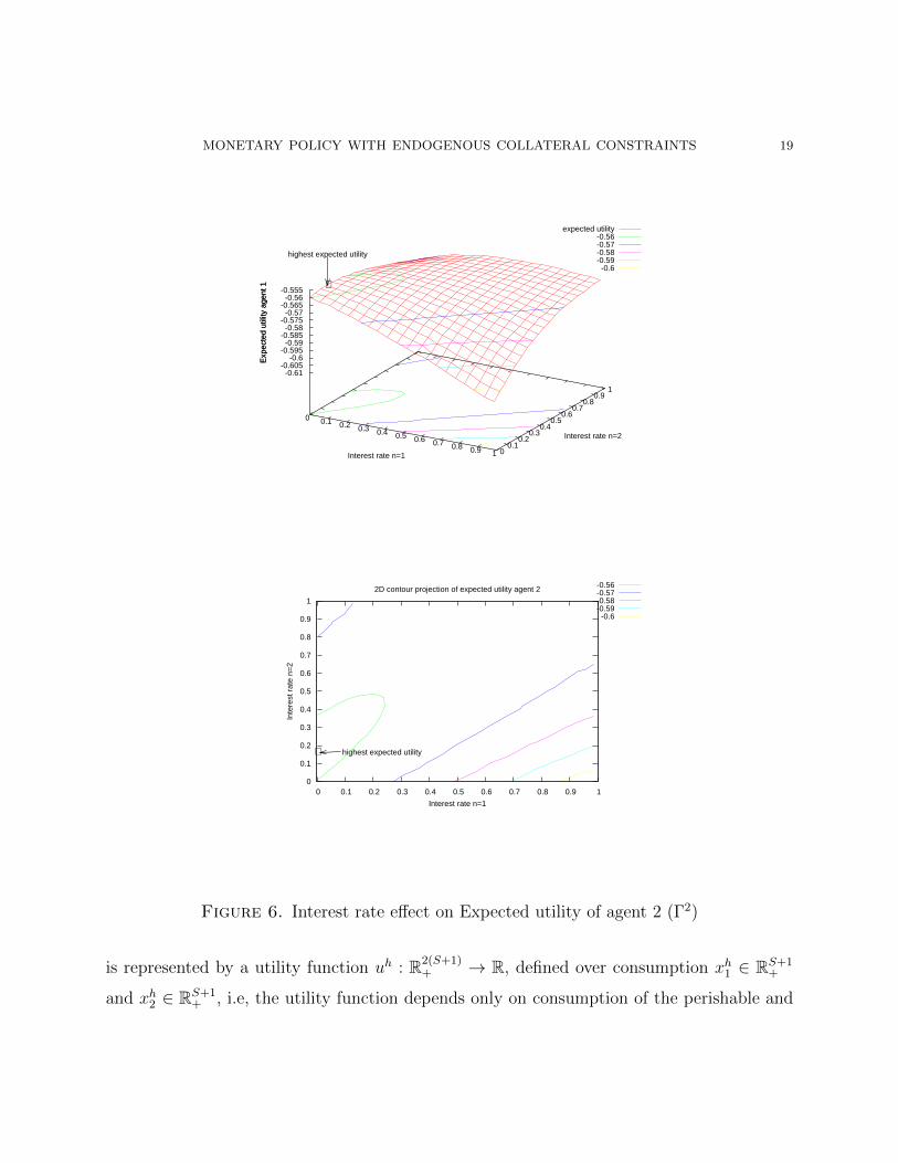
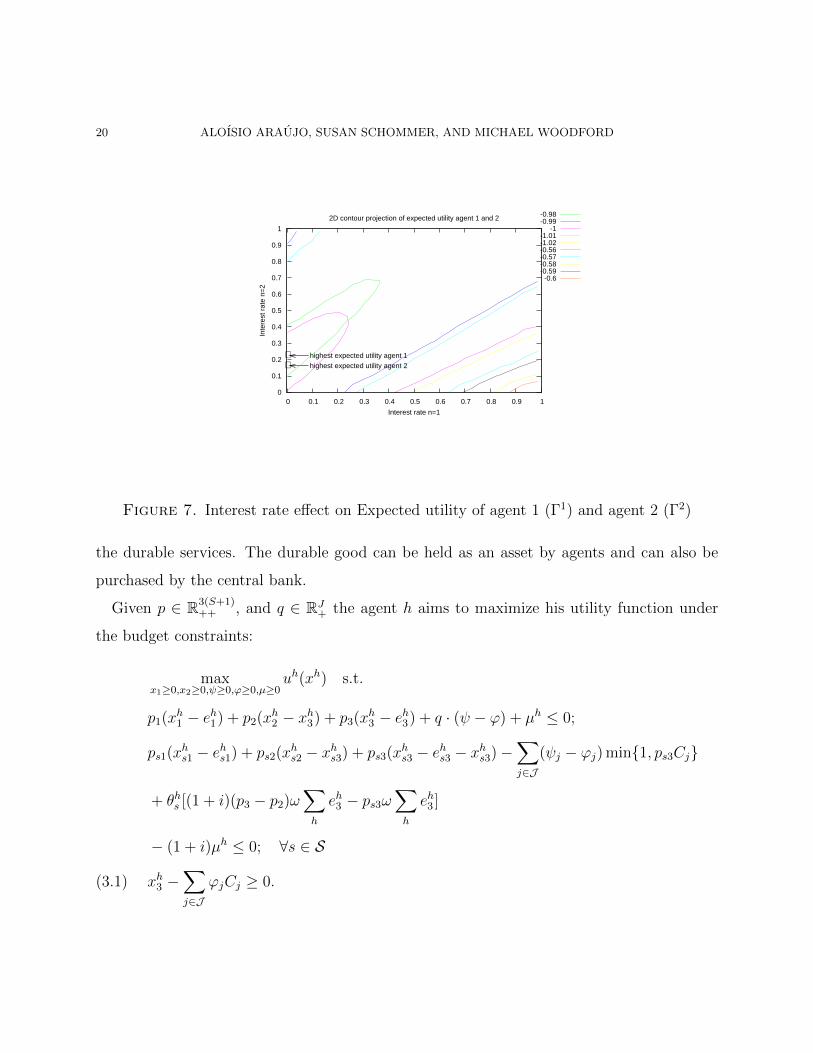
MONETARY POLICY WITH ENDOGENOUS COLLATERAL CONSTRAINTS 17
with the contours for both households in the same plane is the Figure 7. In this example,
for the first state the optimal policy is a zero interest rate. It is especially interesting in this
case to consider an alternative instrument of monetary policy.
3. A finite horizon model with two dimensions of monetary policy
We now include the possibility of purchases of the collateralizable durable good by the
central bank, which could be particularly interesting to implement when the interest rate
reaches the zero lower bound (as we show in the example above in the section 2.2.3). First,
we show when this alternative monetary policy has effect on the equilibrium allocations of
resources, in a two period model with flexible prices. Moreover, we examine a flexible prices
three period model with purchases of the collateralizable durable good by the central bank
in different states in the second period.
3.1. A simple case. We modify the model presented in section 2.1 to include a rental
market for durable services and purchases of the collateralizable durable good by the central
bank. In this version of the model, there are three goods l ∈ L = {1, 2, 3} where good 1
is perishable, good 2 is [rental of] durable services and good 3 is [purchases of] the durable
good. We assume that it is possible to store only the durable good and that there is no
depreciation.
The central bank can purchase durable good in the first period, in an amount given by
ω∑
h eh3 where ω ∈ (0, 1] represents the fraction of aggregate durable good supply purchased
by the central bank. The central bank also issues money in the amount needed to pay for
these purchases, so that M = (p3 − p2)ω∑
h eh3 . The net tax obligation of household h in
state s in the second period is
θhs [(1 + i)(p3 − p2)ω∑h
eh3 − ps3ω∑h
eh3 ],
where the quantity in square brackets is the amount by which the amount owed by the
central bank on its liabilities exceeds the value of its assets.
18 ALOISIO ARAUJO, SUSAN SCHOMMER, AND MICHAEL WOODFORD
0 0.1 0.2 0.3 0.4 0.5 0.6 0.7 0.8 0.9 1 0 0.1
0.2 0.3
0.4 0.5
0.6 0.7
0.8 0.9
1
-1.03
-1.02
-1.01
-1
-0.99
-0.98
-0.97
Exp
ecte
d ut
ility
age
nt 1 ∗
highest expected utility
expected utility -0.98 -0.99
-1 -1.01 -1.02
Interest rate n=1
Interest rate n=2
Exp
ecte
d ut
ility
age
nt 1
2D contour projection of expected utility agent 1
∗ highest expected utility
-0.98 -0.99
-1 -1.01 -1.02
0 0.1 0.2 0.3 0.4 0.5 0.6 0.7 0.8 0.9 1
Interest rate n=1
0
0.1
0.2
0.3
0.4
0.5
0.6
0.7
0.8
0.9
1
Inte
rest
rat
e n=
2
Figure 5. Interest rate effect on Expected utility of agent 1 (Γ1)
Each agent has an endowment of the goods (only non-zero for the perishable and the
durable goods) in each period and state, eh ∈ R2(S+1)+ . The preference ordering of agent h
MONETARY POLICY WITH ENDOGENOUS COLLATERAL CONSTRAINTS 19
0 0.1 0.2 0.3 0.4 0.5 0.6 0.7 0.8 0.9 1 0 0.1
0.2 0.3
0.4 0.5
0.6 0.7
0.8 0.9
1
-0.61-0.605
-0.6-0.595
-0.59-0.585
-0.58-0.575
-0.57-0.565
-0.56-0.555
Exp
ecte
d ut
ility
age
nt 1 ∗
highest expected utility
expected utility -0.56 -0.57 -0.58 -0.59 -0.6
Interest rate n=1
Interest rate n=2
Exp
ecte
d ut
ility
age
nt 1
2D contour projection of expected utility agent 2
∗ highest expected utility
-0.56 -0.57 -0.58 -0.59 -0.6
0 0.1 0.2 0.3 0.4 0.5 0.6 0.7 0.8 0.9 1
Interest rate n=1
0
0.1
0.2
0.3
0.4
0.5
0.6
0.7
0.8
0.9
1
Inte
rest
rat
e n=
2
Figure 6. Interest rate effect on Expected utility of agent 2 (Γ2)
is represented by a utility function uh : R2(S+1)+ → R, defined over consumption xh1 ∈ RS+1
+
and xh2 ∈ RS+1+ , i.e, the utility function depends only on consumption of the perishable and
20 ALOISIO ARAUJO, SUSAN SCHOMMER, AND MICHAEL WOODFORD
2D contour projection of expected utility agent 1 and 2
∗ highest expected utility agent 1∗ highest expected utility agent 2
-0.98 -0.99
-1 -1.01 -1.02 -0.56 -0.57 -0.58 -0.59 -0.6
0 0.1 0.2 0.3 0.4 0.5 0.6 0.7 0.8 0.9 1
Interest rate n=1
0
0.1
0.2
0.3
0.4
0.5
0.6
0.7
0.8
0.9
1
Inte
rest
rat
e n=
2
Figure 7. Interest rate effect on Expected utility of agent 1 (Γ1) and agent 2 (Γ2)
the durable services. The durable good can be held as an asset by agents and can also be
purchased by the central bank.
Given p ∈ R3(S+1)++ , and q ∈ RJ
+ the agent h aims to maximize his utility function under
the budget constraints:
maxx1≥0,x2≥0,ψ≥0,ϕ≥0,µ≥0
uh(xh) s.t.
p1(xh1 − eh1) + p2(x
h2 − xh3) + p3(x
h3 − eh3) + q · (ψ − ϕ) + µh ≤ 0;
ps1(xhs1 − ehs1) + ps2(x
hs2 − xhs3) + ps3(x
hs3 − ehs3 − xhs3)−
∑j∈J
(ψj − ϕj) min{1, ps3Cj}
+ θhs [(1 + i)(p3 − p2)ω∑h
eh3 − ps3ω∑h
eh3 ]
− (1 + i)µh ≤ 0; ∀s ∈ S
xh3 −∑j∈J
ϕjCj ≥ 0.(3.1)
MONETARY POLICY WITH ENDOGENOUS COLLATERAL CONSTRAINTS 21
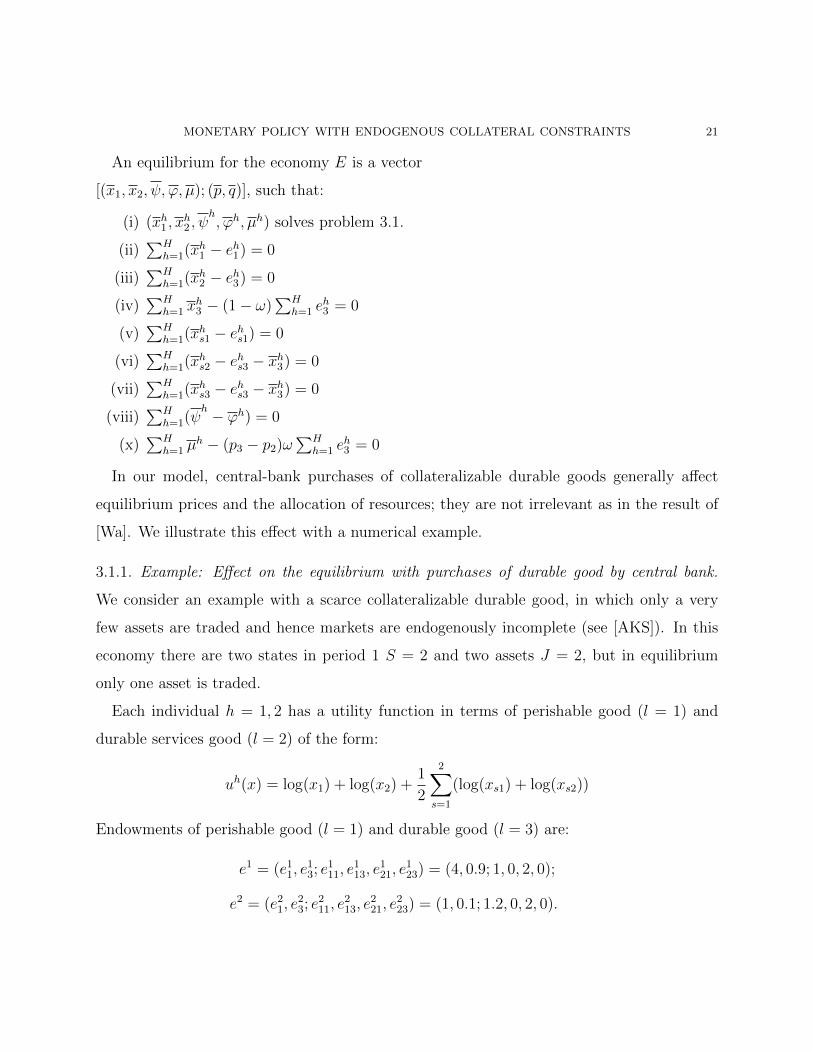
An equilibrium for the economy E is a vector
[(x1, x2, ψ, ϕ, µ); (p, q)], such that:
(i) (xh1 , xh2 , ψ
h, ϕh, µh) solves problem 3.1.
(ii)∑H
h=1(xh1 − eh1) = 0
(iii)∑H
h=1(xh2 − eh3) = 0
(iv)∑H
h=1 xh3 − (1− ω)
∑Hh=1 e
h3 = 0
(v)∑H
h=1(xhs1 − ehs1) = 0
(vi)∑H
h=1(xhs2 − ehs3 − xh3) = 0
(vii)∑H
h=1(xhs3 − ehs3 − xh3) = 0
(viii)∑H
h=1(ψh − ϕh) = 0
(x)∑H
h=1 µh − (p3 − p2)ω
∑Hh=1 e
h3 = 0
In our model, central-bank purchases of collateralizable durable goods generally affect
equilibrium prices and the allocation of resources; they are not irrelevant as in the result of
[Wa]. We illustrate this effect with a numerical example.
3.1.1. Example: Effect on the equilibrium with purchases of durable good by central bank.
We consider an example with a scarce collateralizable durable good, in which only a very
few assets are traded and hence markets are endogenously incomplete (see [AKS]). In this
economy there are two states in period 1 S = 2 and two assets J = 2, but in equilibrium
only one asset is traded.
Each individual h = 1, 2 has a utility function in terms of perishable good (l = 1) and
durable services good (l = 2) of the form:
uh(x) = log(x1) + log(x2) +1
2
2∑s=1
(log(xs1) + log(xs2))
Endowments of perishable good (l = 1) and durable good (l = 3) are:
e1 = (e11, e13; e
111, e
113, e
121, e
123) = (4, 0.9; 1, 0, 2, 0);
e2 = (e21, e23; e
211, e
213, e
221, e
223) = (1, 0.1; 1.2, 0, 2, 0).
22 ALOISIO ARAUJO, SUSAN SCHOMMER, AND MICHAEL WOODFORD
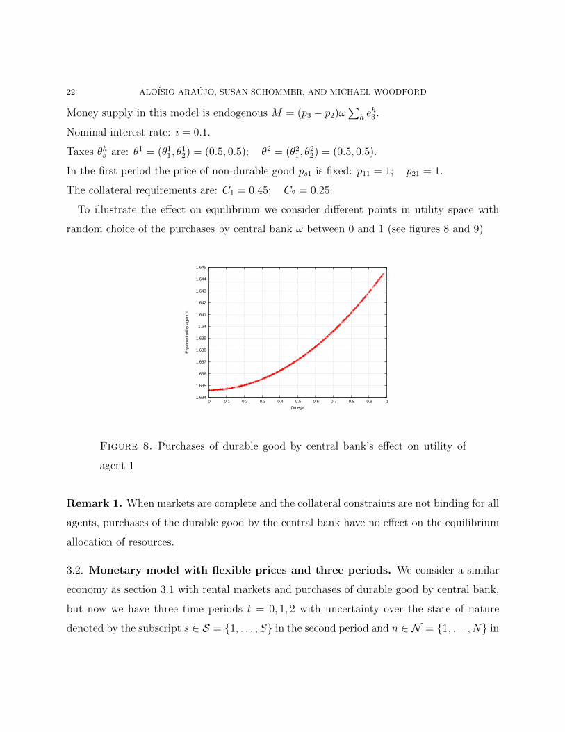
Money supply in this model is endogenous M = (p3 − p2)ω∑
h eh3 .
Nominal interest rate: i = 0.1.
Taxes θhs are: θ1 = (θ11, θ12) = (0.5, 0.5); θ2 = (θ21, θ
22) = (0.5, 0.5).
In the first period the price of non-durable good ps1 is fixed: p11 = 1; p21 = 1.
The collateral requirements are: C1 = 0.45; C2 = 0.25.
To illustrate the effect on equilibrium we consider different points in utility space with
random choice of the purchases by central bank ω between 0 and 1 (see figures 8 and 9)
1.634
1.635
1.636
1.637
1.638
1.639
1.64
1.641
1.642
1.643
1.644
1.645
0 0.1 0.2 0.3 0.4 0.5 0.6 0.7 0.8 0.9 1
Exp
ecte
d ut
ility
age
nt 1
Omega
Figure 8. Purchases of durable good by central bank’s effect on utility of
agent 1
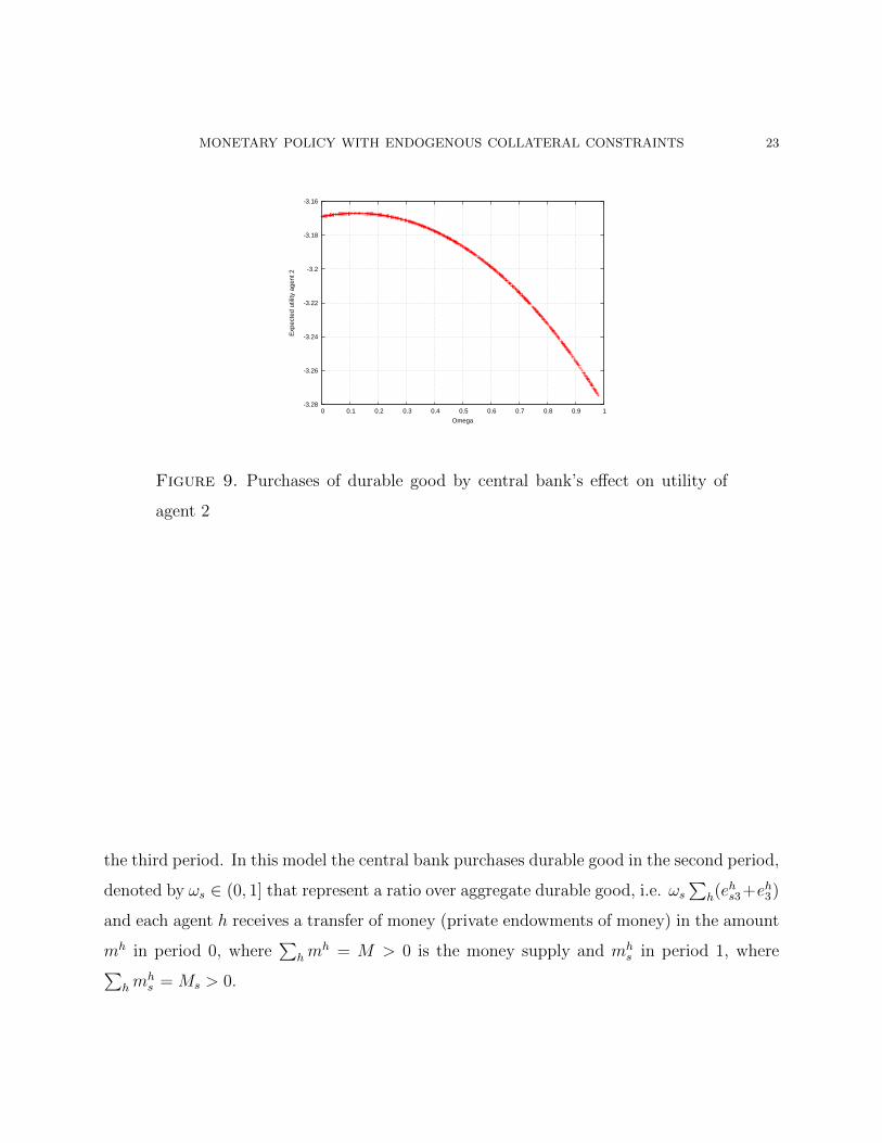
Remark 1. When markets are complete and the collateral constraints are not binding for all
agents, purchases of the durable good by the central bank have no effect on the equilibrium
allocation of resources.
3.2. Monetary model with flexible prices and three periods. We consider a similar
economy as section 3.1 with rental markets and purchases of durable good by central bank,
but now we have three time periods t = 0, 1, 2 with uncertainty over the state of nature
denoted by the subscript s ∈ S = {1, . . . , S} in the second period and n ∈ N = {1, . . . , N} in
MONETARY POLICY WITH ENDOGENOUS COLLATERAL CONSTRAINTS 23
-3.28
-3.26
-3.24
-3.22
-3.2
-3.18
-3.16
0 0.1 0.2 0.3 0.4 0.5 0.6 0.7 0.8 0.9 1
Exp
ecte
d ut
ility
age
nt 2
Omega
Figure 9. Purchases of durable good by central bank’s effect on utility of
agent 2
the third period. In this model the central bank purchases durable good in the second period,
denoted by ωs ∈ (0, 1] that represent a ratio over aggregate durable good, i.e. ωs∑
h(ehs3+eh3)
and each agent h receives a transfer of money (private endowments of money) in the amount
mh in period 0, where∑
hmh = M > 0 is the money supply and mh
s in period 1, where∑hm
hs = Ms > 0.
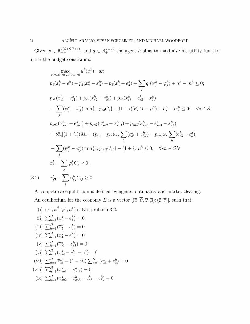
24 ALOISIO ARAUJO, SUSAN SCHOMMER, AND MICHAEL WOODFORD
Given p ∈ R3(S+SN+1)++ , and q ∈ RJ+SJ
+ the agent h aims to maximize his utility function
under the budget constraints:
maxx≥0,ψ≥0,ϕ≥0,µ≥0
uh(xh) s.t.
p1(xh1 − eh1) + p2(x
h2 − xh3) + p3(x
h3 − eh3) +
∑j
qj(ψhj − ϕhj ) + µh −mh ≤ 0;
ps1(xhs1 − ehs1) + ps2(x
hs2 − xhs3) + ps3(x
hs3 − ehs3 − xh3)
−∑j
(ψhj − ϕhj ) min{1, ps3Cj}+ (1 + i)(θhsM − µh) + µhs −mhs ≤ 0; ∀s ∈ S
psn1(xhsn1 − ehsn1) + psn2(x
hsn2 − xhsn3) + psn3(x
hsn3 − ehsn3 − xhs3)
+ θhsn[(1 + is)(Ms + (ps3 − ps2)ωs∑h
(ehs3 + eh3))− psn3ωs∑h
(ehs3 + eh3)]
−∑j
(ψhj − ϕhj ) min{1, psn3Csj} − (1 + is)µhs ≤ 0; ∀sn ∈ SN
xh3 −∑j
ϕhjCj ≥ 0;
xhs3 −∑j
ϕhsjCsj ≥ 0.(3.2)
A competitive equilibrium is defined by agents’ optimality and market clearing.
An equilibrium for the economy E is a vector [(x, ψ, ϕ, µ); (p, q)], such that:
(i) (xh, ψh, ϕh, µh) solves problem 3.2.
(ii)∑H
h=1(xh1 − eh1) = 0
(iii)∑H
h=1(xh2 − eh3) = 0
(iv)∑H
h=1(xh3 − eh3) = 0
(v)∑H
h=1(xhs1 − ehs1) = 0
(vi)∑H
h=1(xhs2 − ehs3 − eh3) = 0
(vii)∑H
h=1 xhs3 − (1− ωs)
∑Hh=1(e
hs3 + eh3) = 0
(viii)∑H
h=1(xhsn1 − ehsn1) = 0
(ix)∑H
h=1(xhsn2 − ehsn3 − ehs3 − eh3) = 0
MONETARY POLICY WITH ENDOGENOUS COLLATERAL CONSTRAINTS 25
(x)∑H
h=1(xhsn3 − ehsn3 − ehs3 − eh3) = 0
(xi)∑H
h=1(ψh
j − ϕhj ) = 0
(xii)∑H
h=1(ψh
sj − ϕhsj) = 0
(xiii)∑H
h=1 µh −M = 0
(xiv)∑H
h=1 µhs −Ms − (ps3 − ps2)ωs
∑Hh=1(e
hs3 − eh3) = 0
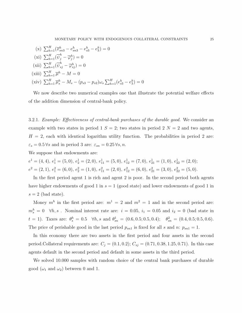
We now describe two numerical examples one that illustrate the potential welfare effects
of the addition dimension of central-bank policy.
3.2.1. Example: Effectiveness of central-bank purchases of the durable good. We consider an
example with two states in period 1 S = 2; two states in period 2 N = 2 and two agents,
H = 2, each with identical logarithm utility function. The probabilities in period 2 are:
εs = 0.5 ∀s and in period 3 are: εsn = 0.25∀s, n.
We suppose that endowments are:
e1 = (4, 4), e11 = (5, 0), e12 = (2, 0), e111 = (5, 0), e112 = (7, 0), e121 = (1, 0), e122 = (2, 0);
e2 = (2, 1), e21 = (6, 0), e22 = (1, 0), e211 = (2, 0), e212 = (6, 0), e221 = (3, 0), e222 = (5, 0).
In the first period agent 1 is rich and agent 2 is poor. In the second period both agents
have higher endowments of good 1 in s = 1 (good state) and lower endowments of good 1 in
s = 2 (bad state).
Money mh in the first period are: m1 = 2 and m2 = 1 and in the second period are:
mhs = 0 ∀h, s . Nominal interest rate are: i = 0.05, i1 = 0.05 and i2 = 0 (bad state in
t = 1). Taxes are: θhs = 0.5 ∀h, s and θ1sn = (0.6, 0.5; 0.5, 0.4); θ2sn = (0.4, 0.5; 0.5, 0.6).
The price of perishable good in the last period psn1 is fixed for all s and n: psn1 = 1.
In this economy there are two assets in the first period and four assets in the second
period.Collateral requirements are: Cj = (0.1, 0.2); Csj = (0.71, 0.38, 1.25, 0.71). In this case
agents default in the second period and default in some assets in the third period.
We solved 10.000 samples with random choice of the central bank purchases of durable
good (ω1 and ω2) between 0 and 1.
26 ALOISIO ARAUJO, SUSAN SCHOMMER, AND MICHAEL WOODFORD
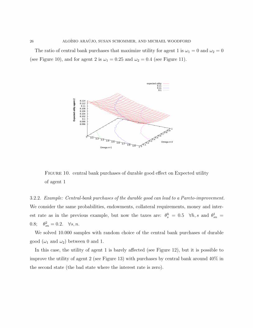
The ratio of central bank purchases that maximize utility for agent 1 is ω1 = 0 and ω2 = 0
(see Figure 10), and for agent 2 is ω1 = 0.25 and ω2 = 0.4 (see Figure 11).
0 0.1 0.2 0.3 0.4 0.5 0.6 0.7 0.8 0.9 1 0 0.1
0.2 0.3
0.4 0.5
0.6 0.7
0.8 0.9
1
8.096 8.098
8.1 8.102 8.104 8.106 8.108 8.11
8.112 8.114
Exp
ecte
d ut
ility
age
nt 2
expected utility 8.11 8.11 8.1
Omega n=1
Omega n=2
Exp
ecte
d ut
ility
age
nt 2
Figure 10. central bank purchases of durable good effect on Expected utility
of agent 1
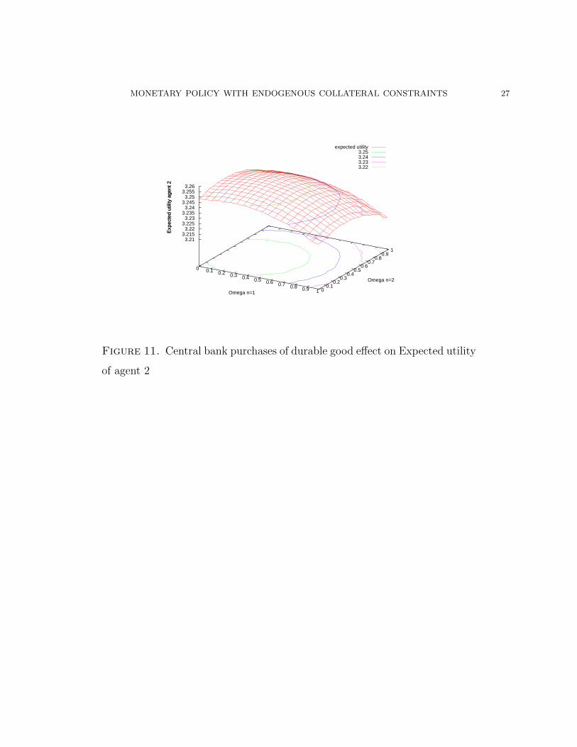
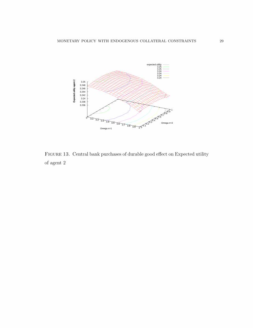
3.2.2. Example: Central-bank purchases of the durable good can lead to a Pareto-improvement.
We consider the same probabilities, endowments, collateral requirements, money and inter-
est rate as in the previous example, but now the taxes are: θhs = 0.5 ∀h, s and θ1sn =
0.8; θ2sn = 0.2. ∀s, n.
We solved 10.000 samples with random choice of the central bank purchases of durable
good (ω1 and ω2) between 0 and 1.
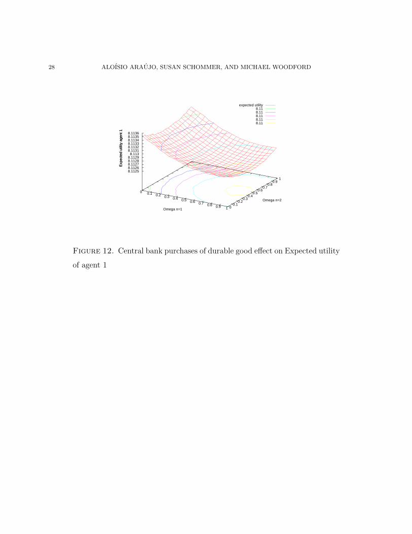
In this case, the utility of agent 1 is barely affected (see Figure 12), but it is possible to
improve the utility of agent 2 (see Figure 13) with purchases by central bank around 40% in
the second state (the bad state where the interest rate is zero).
MONETARY POLICY WITH ENDOGENOUS COLLATERAL CONSTRAINTS 27
0 0.1 0.2 0.3 0.4 0.5 0.6 0.7 0.8 0.9 1 0 0.1
0.2 0.3
0.4 0.5
0.6 0.7
0.8 0.9
1
3.21 3.215 3.22
3.225 3.23
3.235 3.24
3.245 3.25
3.255 3.26
Exp
ecte
d ut
ility
age
nt 2
expected utility 3.25 3.24 3.23 3.22
Omega n=1
Omega n=2
Exp
ecte
d ut
ility
age
nt 2
Figure 11. Central bank purchases of durable good effect on Expected utility
of agent 2
28 ALOISIO ARAUJO, SUSAN SCHOMMER, AND MICHAEL WOODFORD
0 0.1 0.2 0.3 0.4 0.5 0.6 0.7 0.8 0.9 1 0 0.1
0.2 0.3
0.4 0.5
0.6 0.7
0.8 0.9
1
8.1125 8.1126 8.1127 8.1128 8.1129
8.113 8.1131 8.1132 8.1133 8.1134 8.1135 8.1136
Exp
ecte
d ut
ility
age
nt 1
expected utility 8.11 8.11 8.11 8.11 8.11
Omega n=1
Omega n=2
Exp
ecte
d ut
ility
age
nt 1
Figure 12. Central bank purchases of durable good effect on Expected utility
of agent 1
MONETARY POLICY WITH ENDOGENOUS COLLATERAL CONSTRAINTS 29
0 0.1 0.2 0.3 0.4 0.5 0.6 0.7 0.8 0.9 1 0 0.1
0.2 0.3
0.4 0.5
0.6 0.7
0.8 0.9
1
3.236
3.238
3.24
3.242
3.244
3.246
3.248
3.25
Exp
ecte
d ut
ility
age
nt 2
expected utility 3.25 3.25 3.24 3.24 3.24 3.24
Omega n=1
Omega n=2
Exp
ecte
d ut
ility
age
nt 2
Figure 13. Central bank purchases of durable good effect on Expected utility
of agent 2
30 ALOISIO ARAUJO, SUSAN SCHOMMER, AND MICHAEL WOODFORD
References
[AKS] A. Araujo, F. Kubler and S. Schommer. Regulating collateral when markets are incomplete. To appear
in Journal of Economic Theory.
[CWo] V. Curdia, M. Woodford, The central-bank balance sheet as an instrument of monetary policy, NBER
Working Paper no. 16208, July 2010.
[GZ] J. Geanakoplos, W. Zame, Collateralized Asset Markets, 2007.
[Wa] N. Wallace. A Modigliani-Miller theorem for open-market operations. American Economic Review, 71
(1981), 267–274.
[Wo] M. Woodford, Interest and Prices: Foundations of a Theory of Monetary Policy, Princeton University
Press, 2003.
Aloısio Araujo, IMPA and EPGE-FGV
Susan Schommer, IMPA
Michael Woodford, Columbia University