Controls Laboratory Report. Control of a Heater Element Using a LabVIEW-Based PID Controller.

Control of a Heater Element Using a LabVIEW-Based PID Controller

By: Bradly Gassner

ME4480: Control Systems Laboratory

TA: Austin Sutton

October 14, 2015

Abstract

A PID controller implemented in LabVIEW was used to control a small heater. The project proceeded

in two distinct phases: tutorials and PID heater controller itself. Nine tutorials were followed and are

outlined and discussed in this report. The heater controller project fell into three separate sections: P

(proportional) controller integration, I (integral) controller integration, and D (derivative) controller

integration. The resulting PID controller was used to quickly achieve and maintain a desired set point

temperature.

I. Introduction LabVIEW is an icon-based visual programming language for the Windows operating system. The

purpose of the following tutorials and project is to learn about some of the capabilities of the LabVIEW

system and to perform simple data acquisition tasks. Tutorials 1 through 5 provide an introduction to

many of the visual programming features and functions of the LabVIEW environment. Tutorials 6 and 7

use the external Wavetek function generator as a source for some simple data acquisition using the

PCI1200 data acquisition board. Finally, Tutorial 8 deals with using the LabVIEW system to output data.

Following the completion of the tutorials, a project was undertaken to implement a PID controller to

operate a small heater.

II. Laboratory Work The hardware used in the completion of the exercises includes an Intel Core 2 Duo CPU computer

running LabVIEW and Microsoft Excel on Microsoft Windows, a Wavetek FG2A function generator, a

DC- and stepper-motor display with variable resistor feedback, a PCI 1200 data acquisition card, a small

heater setup with temperature feedback, and a myDAQ data acquisition and analog/digital output board.

The use of the hardware other than the heater setup i.e., tutorials, is discussed in detail below in

section III.

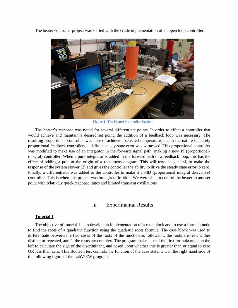
The heater controller project was started with the crude implementation of an open loop controller.

Figure 1: The Heater Controller Station

The heater’s response was noted for several different set points. In order to affect a controller that

would achieve and maintain a desired set point, the addition of a feedback loop was necessary. The

resulting proportional controller was able to achieve a selected temperature, but in the nature of purely

proportional feedback controllers, a definite steady-state error was witnessed. This proportional controller

was modified to make use of an integrator in the forward signal path, making a new PI (proportional-

integral) controller. When a pure integrator is added in the forward path of a feedback loop, this has the

effect of adding a pole at the origin of a root locus diagram. This will tend, in general, to make the

response of the system slower [2] and gives the controller the ability to drive the steady state error to zero.

Finally, a differentiator was added to the controller to make it a PID (proportional integral derivative)

controller. This is where the project was brought to fruition. We were able to control the heater to any set

point with relatively quick response times and limited transient oscillations.

III. Experimental Results

Tutorial 1

The objective of tutorial 1 is to develop an implementation of a case block and to use a formula node

to find the roots of a quadratic function using the quadratic roots formula. The case block was used to

differentiate between the two cases of the roots of the function as follows: 1. the roots are real, wither

distinct or repeated, and 2. the roots are complex. The program makes use of the first formula node on the

left to calculate the sign of the discriminant, and based upon whether this is greater than or equal to zero

OR less than zero. This Boolean test controls the function of the case statement in the right hand side of

the following figure of the LabVIEW program.

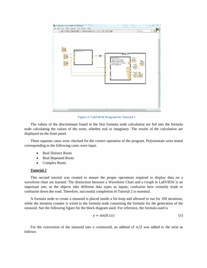
Figure 2: LabVIEW Program for Tutorial 1

The values of the discriminant found in the first formula node calculation are fed into the formula

node calculating the values of the roots, whether real or imaginary. The results of the calculation are

displayed on the front panel.

Three separate cases were checked for the correct operation of the program. Polynomials were tested

corresponding to the following cases were input.

Real Distinct Roots

Real Repeated Roots

Complex Roots

Tutorial 2

This second tutorial was created to ensure the proper operations required to display data on a

waveform chart are learned. The distinction between a Waveform Chart and a Graph in LabVIEW is an

important one, as the objects take different data types as inputs; confusion here certainly leads to

confusion down the road. Therefore, successful completion of Tutorial 2 is essential.

A formula node to create a sinusoid is placed inside a for-loop and allowed to run for 100 iterations,

while the iteration counter is wired to the formula node containing the formula for the generation of the

sinusoid. See the following figure for the block diagram used. For reference, the formula used is

𝑦 = sin(0.1𝑥) (1)

For the conversion of the sinusoid into a cosinusoid, an addend of 𝜋/2 was added to the term as

follows:

𝑦 = sin(0.1𝑥 +𝜋

2) (2)

Figure 3: Tutorial 2 Block Diagram

Figure 4: Waveform Chart for Tutorial 2, sinusoid

The scaling factor was required in the formula to ensure a continuous-looking function. Imagine if

one tried to plot sin(1) , sin(2) , … , sin(𝑛). The period of the generated function would be much too high

to be comprehensible. It may look pretty.

Upon changing the size of the scaling factor, the plot is indeed changed due to the fact that the period

of the resulting sinusoid is changed.

The length of the data displayed on the waveform chart will be different if the number of points to be

plotted is changed (the iteration specifier on the for-loop). More or fewer periods will be shown.

Tutorial 3

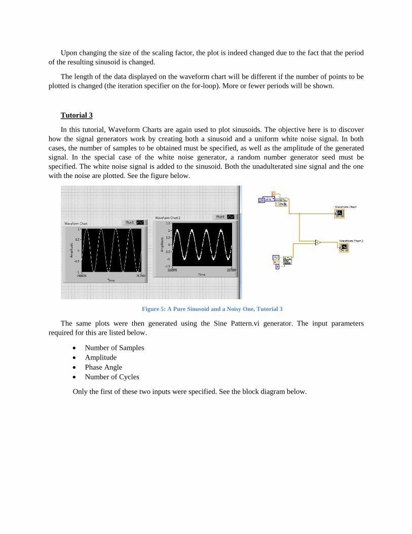
In this tutorial, Waveform Charts are again used to plot sinusoids. The objective here is to discover

how the signal generators work by creating both a sinusoid and a uniform white noise signal. In both

cases, the number of samples to be obtained must be specified, as well as the amplitude of the generated

signal. In the special case of the white noise generator, a random number generator seed must be

specified. The white noise signal is added to the sinusoid. Both the unadulterated sine signal and the one

with the noise are plotted. See the figure below.

Figure 5: A Pure Sinusoid and a Noisy One, Tutorial 3

The same plots were then generated using the Sine Pattern.vi generator. The input parameters

required for this are listed below.

Number of Samples

Amplitude

Phase Angle

Number of Cycles

Only the first of these two inputs were specified. See the block diagram below.

Figure 6: Using a Sine Pattern.vi to Generate a Signal, Tutorial 3

The element-wise nature of the addition operator used displays some unexpected results that were

explored in the execution of this tutorial. If two arrays are fed into the addition operator as above, the

operator returns a result array that is of a length that is the shorter of the two lengths of the inputs. It will

simply truncate the results of the output array to match the shortest input. Let’s call this the “minimum

array size truncation property.” This is a bit counterintuitive, as one would expect perhaps that the

remaining unmatched elementwise sums to simply be the input plus zero. It is important to keep this in

mind: another simple LabVIEW idiosyncrasy that could cost hours if it catches one unaware.

Tutorial 4

In what is arguably the most enjoyable tutorial yet, Tutorial 4 involves the simulation of a linear first-

order differential system to an impulse input. The objective of this exercise is manifold: review first order

system response simulation, plots, transfer functions, and learn a few new LabVIEW operators, including

the In Range object, bundle, and XY graphs.

A first-order differential system is governed by the equation

�̇�(𝑡) + 𝑦(𝑡) = 𝑢(𝑡) (3)

The derivative is approximated by a discrete form given in the lab manual [1], and rearranged (see

equation 3.8, p. 52) to give us a form of the differential equation that we may use with a formula node,

iteratively stepping through the solution.

𝑦(𝑘 + 1) = 𝑦(𝑘) + ∆𝑡(𝑢(𝑘) − 𝑦(𝑘)) (4)

See the following block diagram, Figure 7: Tutorial 4 Block Diagram, to reference during our

discussion of the operation of the program.

Figure 7: Tutorial 4 Block Diagram

The main body of the program is enclosed in a large for-loop. This is set to N iterations. Initial

conditions are specified on the left side of the for-loop as initial inputs to the shift registers. The upper

shift register contains the history of the variable Yorg, which is the initial condition during the first

iteration and subsequently the continuous previous iteration of y(t). The lower shift register contains the

history of t0, the initial value during the first iteration (-0.5), and subsequently the continuous previous

iteration of t. The operation of the program depends up on the value of t. The In Range? Object compares

the current value of the time variable to a lower and upper limit of −0.01 < 𝑡 < 0.01. For the single

iteration in which the value of the time variable t falls within that range, i.e. that value is identically zero,

the In Range? Object returns a true value to the case block. While this Boolean input is true, the input

𝑢(𝑡) is set to a value of 0.5. This is the impulse input, since in the following iteration, the value of t is no

longer ‘in range’ and the false case is executed. In the false case of the case block, the input is set to zero.

It is in this way to which the solution to the differential equation is arrived. Marching through the

differential space blindly, step by step. At the culmination of the for-loop’s iterations, the arrays for the

variables t, y, and u are fully filled. It is here that we learn of another LabVIEW idiosyncrasy. The arrays

must be plotted on XY Graphs, and the axes of these LabVIEW objects are dealt with entirely backward.

The universally accepted ordering of the dependent vs. independent, ordinate vs. abscissa, y vs. x:

LabVIEW throws this out the window and requires bundling the axes with the X array first, then the Y

before being able to display properly on an XY Graph. Keep this in mind when working with LabVIEW

in the future. Much frustration may be prevented.

In any case, the plots of Y vs. t and U vs. t are displayed on the front panel. In order to analyze the

system more carefully, the data were exported and plotted in Excel.

Figure 8: Response of a First-Order Differential System to an Impulse Excitation

It is important to note that the time constant of the system may be obtained by inspection of the

response curve. Using the 37% rule, the response decays to 37% of its peak value in one time constant.

For this system, this time constant is approximately one second.

Tutorial 5

The objective of this tutorial is to simulate the response of another first order dynamic system. Also,

review transfer functions and implement a simple proportional feedback control. The differential equation

describing the system dynamics that is to be simulated is given by

�̇�(𝑡) = 0.2𝑦(𝑡) + 𝑢(𝑡) (5)

The transfer function describing the dynamic system from input to output is

𝑌(𝑠)

𝑈(𝑠)=

1

𝑠 − 0.2

(6)

The discretization of this system is obtained following the same procedure as given in Tutorial 4 and

is

𝑦(𝑘 + 1) = (1 + .02Δ𝑡)𝑦(𝑘) + Δ𝑡𝑢(𝑘) (7)

The original uncompensated system given in the lab manual was simulated and the response curve

can be seen below. The simulation of this differential system follows the same procedure and general

program as implemented in Tutorial 4.

Figure 9: Uncompensated Tutorial 5

Obviously, the response of this system is unstable as the curve of y versus time tends to infinity

exponentially. This is to be expected in any system where the slope of the response is directly and linearly

proportional to the response!

A proportional feedback controller was designed and implemented with the following form:

𝑢(𝑡) = 𝐾𝑦(𝑡), 𝐾 = −1.2 (8)

Refer to the screenshot below to see the response of the system as it driven to zero with the

proportional feedback controller.

Figure 10: The Proportionally Compensated System Response

See below for the same data more clearly represented in an Excel chart. On the chart, an exponential

curve fit is performed with the indicated time constant of approximately𝜏 =1

1.033= 0.968.

Figure 11: Compensated System Response

Tutorial 6

Tutorial 6 is the first tutorial in which we are using LabVIEW to acquire data. The purpose of this

tutorial is to learn how to properly employ the correct sampling frequency as given by the Nyquist

sampling theorem and learn how to develop a simple LabVIEW program to acquire analog data from an

external signal source. We use an external function generator and our myDAQ board. The program used

can be seen below with a graph of the acquired data. The operation of this LabVIEW program is simple

enough; the only thing we need is really the myDAQ read block. The channel is specified to the sample

clock where the sample rate is also specified. The number of samples is input into the read block, and the

resulting array of size n is displayed on a waveform graph.

Figure 12: Tutorial 6 Program

Figure 13: Sampled Sine Waves

In Figure 13: Sampled Sine Waves, it can be seen that we are sampling the same sine wave with two

different sample rates. In the upper graph, labeled Waveform Graph 2, the sample rate is 2000 samples

per second. Here we are sampling a 100 Hertz sine wave from the external function generator. The

Nyquist sampling theorem dictates that any sampling should occur at a frequency of at least a factor of ten

faster than the highest frequency in the analog signal being sampled. Here, a sample rate of 2000 Hertz is

meeting and exceeding the Nyquist specification by a factor of two. In the lower graph, titled Waveform

Graph, the sample rate is a slow 50 Hertz. We have adjusted the number of samples so the two graphs

display the same length of time. The one half sinusoid signal we see here is a result of signal aliasing. The

actual signal is shaped like the upper graph, and the lower graph simply misses the fundamental

frequency being generated by the external function generator due to the fact that the sampling frequency

is so low.

It is possible to measure the frequency of the sine curve from the graph. One may locate a time of a

peak in the signal and name it t1. Then, locate another peek several periods in the future. Let's call the

second peak t2. Count the peaks (periods) between the points selected and call that 𝑛. The frequency is

given by

𝑓 =𝑛

𝑡2 − 𝑡1

(9)

Tutorial 7

In contrast to Tutorial 6, Tutorial 7 is designed to instruct us on obtaining a single data point. The

myDAQ Read block is set to acquire one channel, one sample, and analog double data point. This point

is displayed on a waveform chart, and this process is repeated by the number of times specified in the

iteration counter of the for-loop. The resulting array is passed out of the for-loop and displayed on a

Waveform Graph.

Figure 14: A Time-Indeterminate Data Acquisition System

A 10 Hertz signal was generated with the external function generator and the data was collected by

the program displayed in Figure 14. See below for a screenshot of the data collected. It is particularly

important to note that in this case, it is impossible to calculate the frequency by inspection of the graph.

Due to the fact that no sample rate was specified by the use of a timing block or otherwise, the frequency

of sampling is only controlled by the speed at which the analog one-channel one-sample function can

occur.

Figure 15: A 10Hz Signal

A 1000 Hertz sine wave was generated with the external function generator and the data was input

into this data collection program. See below for a screenshot of the 1000 Hertz signal. While the lab

manual tasks us with checking for aliasing, it should be obvious that the sample generated is oscillating so

quickly that it is impossible to discern any useful information from the waveform chart and wave form

graph generated.

Figure 16: A 1000Hz Signal

It should be particularly useful to note the differences between the waveform chart and the waveform

graph. The waveform chart shows only a fixed number of samples, and receives data in the form of a

stream of scalars, not organized into an array. The waveform graph on the other hand receives its

information in an array. In this program, the array is auto-indexed through a tunnel in the for-loop. The

waveform graph can display any number of data points, only limited by the size of the array that has been

passed.

The waveform graph will not work if its terminal is placed inside the loop of the program. This is due

to the fact that the input to the waveform graphs is an array and not a sequence of scalars as previously

discussed.

Tutorial 8

In this tutorial we are learning how to output an analog signal through the myDAQ. In addition, we

learn two ways to access the output channels in the myDAQ hardware. The first is to specify the analog

output as a constant in DAQmx Create Task block. The second way to access an output channel is to use

the DAQmx Create Virtual Channel VI.

On the myDAQ system board, analog output 0 is connected to analog input 0. The LabVIEW

program shown in Figure 3. 3. 8 on page 61 of the lab manual was constructed and is referenced below.

It is important to note that this scheme of generating a signal is worthless due to the fact that no

timing function is present to instruct the right block on how to do its job. The output of the program may

be seen below.

Figure 17: A Poorly-Timed Signal Generator

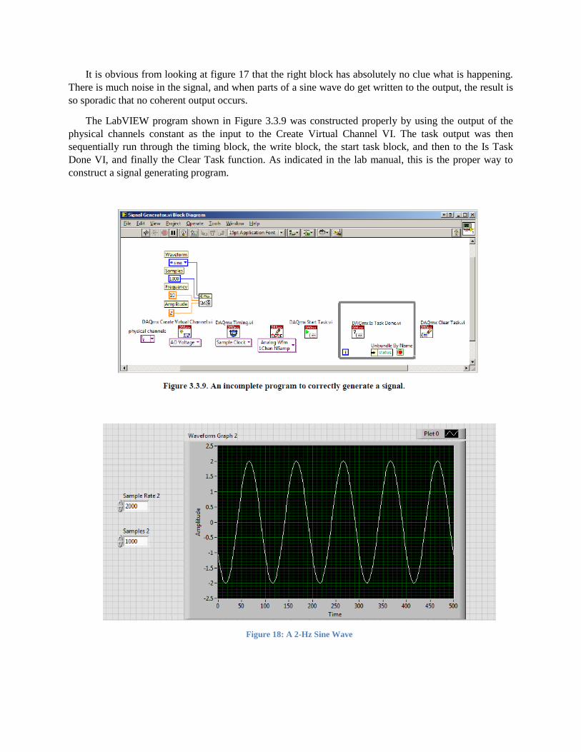
It is obvious from looking at figure 17 that the right block has absolutely no clue what is happening.

There is much noise in the signal, and when parts of a sine wave do get written to the output, the result is

so sporadic that no coherent output occurs.

The LabVIEW program shown in Figure 3.3.9 was constructed properly by using the output of the

physical channels constant as the input to the Create Virtual Channel VI. The task output was then

sequentially run through the timing block, the write block, the start task block, and then to the Is Task

Done VI, and finally the Clear Task function. As indicated in the lab manual, this is the proper way to

construct a signal generating program.

Figure 18: A 2-Hz Sine Wave

Tutorial 9

The objective of tutorial 9 is manifold. First, we learn how to write data as an 8-bit word to a digital

output port. We are using this 8-bit word not as an integer, but as a way to write 8 different values to the

digital output port. In the introduction to this tutorial, we learned about the control of direct current

motors and stepper motors. Unfortunately, the use of the potentiometers specified in the lab manual did

not seem to be working.

They LabVIEW program shown below was constructed to be able to use 8 Boolean switches to write

an 8-bit word to the digital port.

Figure 19: Using Switches to Control a Digital Output Port

As stated above, the potentiometer feedback was out of service. For this reason, it was impossible to

know which direction of the DC motor produced increasing voltage and which direction of the motor

produced a decrease in voltage on the potentiometer purely through experimentation. However, looking at

Figure 4.6.2 below, reproduced from the laboratory manual, it can be seen that in order to produce a

decreasing potentiometer voltage, channel 0 must be off and channel 1 must be on. Conversely, in order

to rotate the motor to provide increasing potentiometer voltage, channel 0 must be on and channel 1 must

be off.

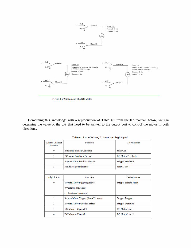
Combining this knowledge with a reproduction of Table 4.1 from the lab manual, below, we can

determine the value of the bits that need to be written to the output port to control the motor in both

directions.

Please see below for the digital bits written and their decimal equivalent for the operation of the DC

motor.

Table 1: Words Written for Motor Control

Direction Pin 0 Pin 1 Pin 2 Pin 3 Pin 4 Binary Word Decimal Equivalent

Increasing Pot V 0 0 0 1 0 01000 8

Decreasing Pot V 0 0 0 0 1 10000 16

LabVIEW Project

In this final portion of the LabVIEW laboratory session, a heater controller was created to allow

control of a small desktop heater which will achieve and maintain a desired temperature set point. The

project preceded in four phases. In part 1, the given code was run for a small range of heater settings

which ranged from 1 to 4 and the temperature at each set point was noted. In this way, referred to as open

loop control, the heater's temperature could be maintained albeit crudely. In part 2, a proportional

controller was added with a feedback loop to be able to set the heater's temperature to a desired value.

The error signal, which is the set temperature minus the current temperature, was multiplied by the

constant of proportionality and this product is the signal that controls the heater. In part 3, and integrator

was added into the forward path of the control loop. This integrator allows a refinement of steady-state

error. Finally, a derivative portion was added to the forward path of the feedback loop to help control

overshoot.

PART 1

The provided program was run for a power setting of three (the setting could range from one to four)

and the temperature of the heater was recorded to be 353℃. See Figure 20: Open Loop Control with

Power Setting 3 for a waveform chart of the heater response to a power setting of 3.

Figure 20: Open Loop Control with Power Setting 3

This power setting was adjusted up and down to gain an understanding of how it controls the

temperature. Here we can see a classic first-order dynamic system response curve. The power setting of

the heater was reduced to two and the response was allowed to even out to more or less a steady state

value. As can be seen in the graphic below, a power setting of 2 corresponds to a steady state heater

temperature of 276 degrees.

Figure 21: Open Loop with a Power Setting of 2

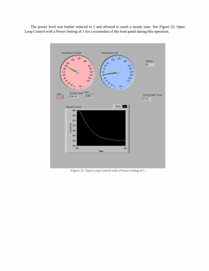
The power level was further reduced to 1 and allowed to reach a steady state. See Figure 22: Open

Loop Control with a Power Setting of 1 for a screenshot of the front panel during this operation.

Figure 22: Open Loop Control with a Power Setting of 1

A short summary of the power settings used and the corresponding steady-state temperature can be

seen in the table below.

Table 2: Heater Power Settings and Steady State Temp

Power Setting Temperature

1 160℃

2 276℃

3 353℃

To be able to control the heater to reach and hold a specific temperature, however, a controller which

uses feedback i.e., a closed loop controller, is necessary.

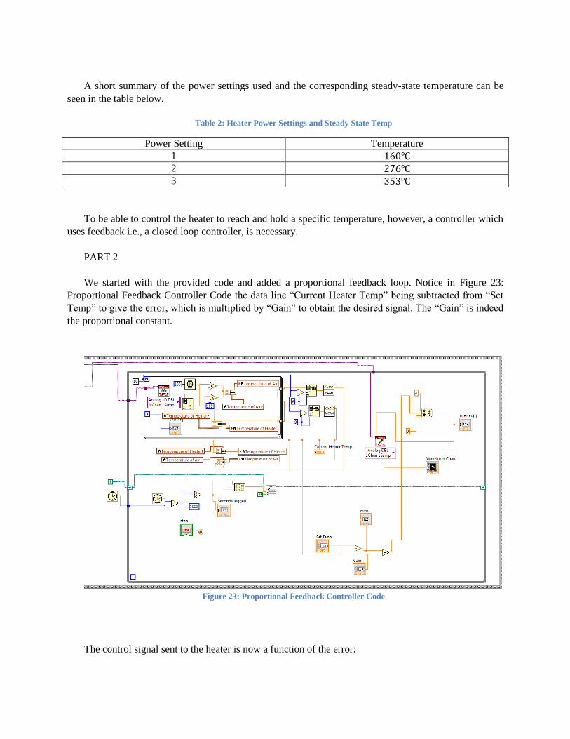
PART 2

We started with the provided code and added a proportional feedback loop. Notice in Figure 23:

Proportional Feedback Controller Code the data line “Current Heater Temp” being subtracted from “Set

Temp” to give the error, which is multiplied by “Gain” to obtain the desired signal. The “Gain” is indeed

the proportional constant.

Figure 23: Proportional Feedback Controller Code

The control signal sent to the heater is now a function of the error:

𝑢 = 𝑘𝑝𝑒 (10)

U is the control signal sent to the heater, ranging from zero to four, and e is the error signal. The In

Range and Coerce block compares the incoming signal (here, u) to the upper and lower bounds specified.

If the signal supplied is outside the bounds, the output is forced to be equal to the upper or lower bound

respectively.

The most effective value for the magnitude of the proportional gain parameter was selected through a

trial and error process. Starting with a gain of unity for a nice baseline response, the system was ran and it

was shown to induce oscillatory behavior in the heater temperature. The following shows this oscillatory

response with the controller set to 200 deg C.

Figure 24: Proportional Gain of 1

In order to reduce the system from one of imaginary poles to one of a more critically damped nature,

the gain was reduced to lower values and the interactive process of finding an appropriate gain started.

See the Table below for the trials, proportional gains, and the responses.

Table 3: Part 2 Proportional Gains and Associated Responses

Run Gain Response

1 1.0 Oscillatory

2 0.75 Oscillatory from 190-205



5 0.1 Overshoot, no oscillation, e_ss=12

6 0.15 No overshoot, e_ss=8

7 0.2 Oscillatory

8 0.18 Little oscillation, e_ss=7

Immediately below is a graph of the heater response for the best setting of the proportional feedback

gain. With a gain equal to 0.18, we see few oscillations and a steady-state error of approximately 7

degrees Celsius.

Figure 25: Our Best Proportional Feedback Controller

PART 3

Part 3 of the heater controller project involves an implementation of a proportional integral controller.

Not only is the error signal being reinforced or attenuated by a proportional constant, we are also

integrating the error signal with respect to time and multiplying that by a constant of integration in the

hopes of reducing the steady-state error.

As can be seen in the block diagram below, the error signal is now being input into a point-by-point

integration block.

Figure 26: A PI Controller

The integral of the error function is then multiplied by a gain, k_i, and this product signal is now

added to the proportional gain to be fed into the controller.

𝑢 = 𝑘𝑝𝑒 + 𝑘𝑖∫𝑒 𝑑𝑡 (11)

Using the best k_p of 0.18 obtained from the optimization of the proportional controller, different

k_i’s were selected until the best response was achieved. At this point, in trial number six, the value of

k_p was changed until obtaining a very nice quick transient and low error steady-state response. Please

see the table below for an overview of the trials completed, the associated constant of proportionality and

integration, and the response characteristics.

Table 4: PI Controller Trials and Constants

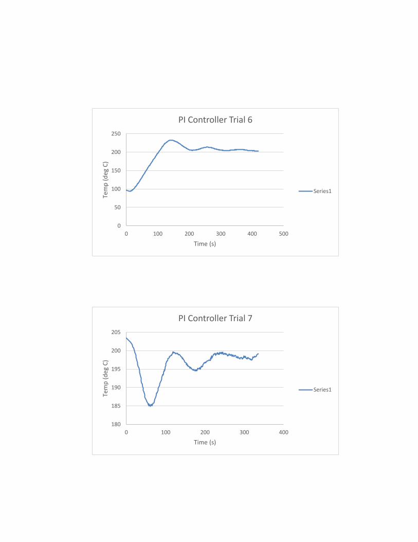
Figure 27: Best PI Response

After obtaining the best transient and steady-state response possible with the constant shown above

for the proportional and integral controller, the controller was set to a different set point, namely 300

degrees Celsius, and turned on at this new set point to investigate the response. Please see the chart below

for the data obtained from this trial.

Figure 28: PI Controller Set to 300C

It can be seen from the chart that the heater which was originally set at 200 degrees C started a steady

linear rise up to approximately 320 degrees C, where the response entered a very short oscillatory phase

before settling quickly to 300 degrees C with negligible steady-state error. This is the response that we

were looking for and we're happy to see. It is obvious from the temperature response curves that the

addition of the integral controller to the proportional controller has had a significant effect on the steady-

state error.

In order to reduce the transient response even further, a derivative portion was implemented into the

proportional-integral controller.

PART 4

As can be seen in the block diagram below, the error is input into a point-by-point differentiation with

respect to time block which is multiplied by a new constant called k_d. This new derivative signal is

added to the proportional and integral feedback signal used previously and is input to the In Range and

Coerce block.

Figure 29: Implementation of a PID Controller

The new formula for the signal applied to the heater can be represented as

𝑢 = 𝑘𝑝𝑒 + 𝑘𝑖∫𝑒 𝑑𝑡 + 𝑘𝑑

𝑑

𝑑𝑡𝑒 (12)

Using the best k_p of 0.18 and k_i of .001 obtained from the optimization of the integral-proportional

controller, different k_d’s were selected until the best response was achieved: obtaining a very nice quick

transient and low error steady-state response. Please see the table below for an overview of the trials

completed, the associated constant of proportionality, integration, and differentiation, and the response

characteristics.

Table 5: PID Controller Multiplier Selection

Figure 30: PID Controller Response Curve

It can be seen from the chart that the heater entered a very short oscillatory phase before settling

quickly to 200 degrees C with negligible steady-state error. Again, this is the response that we were

looking for!

IV. Conclusions

We began this LabVIEW project with 9 tutorials. From the first tutorial which introduced formula

nodes and case structures, to signal generation of sine waves in tutorials 2 and 3. In tutorial four we began

simulation of differential systems. Tutorial 5 introduced a feedback loop and concepts which would be

important in the heater control project to follow. Tutorial 6 gave us the skills necessary to take

measurements of external data and introduced the concept of signal aliasing and the prevention of such

through the use of the Nyquist sampling theorem. Tutorial 7 underscored the need for a timing clock to be

running in the computer during data acquisition. In order to make our data acquisition programs run more

autonomously through the use of dynamic virtual channel creation, Tutorial 8 instructed us on the use of

many DAQmx task blocks. Tutorial 9 helped us understand control of motors through writing to digital

output pins which controlled relays.

While a few of the previous tutorials involve the numerical simulation of a dynamic system, the skills

learned during those tutorials would become useful in the control of an actual, physical system. The

control of a heater progressed through several iterations of control systems. Starting with the open loop

control system, the steady-state temperature response of the heater was noted for varying input levels.

This is the most basic control system. In order to control the heater to maintain a desired set point, a

feedback loop is necessary. In a classical feedback loop, the output reading, i.e. the temperature of the

heater, is subtracted from the desired temperature to obtain an error value. This error value is multiplied

by a constant to obtain the signal that we can use now to drive the heater. Through careful choice of the

proportionality, the error can be scaled in such a way as to enable the feedback loop to maintain the

output temperature to a controlled value.

A simple, straightforward proportional feedback control loop has one glaring flaw. This is the steady-

state error. No matter the value to which we set our error gain, the steady-state error between the set point

and the heater's temperature never got better than 7 degrees Celsius. It is for this reason that the next

iteration of the controller was implemented: the proportional integrator feedback control.

With the use of an integrator in the forward path of the feedback loop, it may be said that we give our

controller a “knowledge of the past.” As the proportional section of the controller maintains a steady state

error, this value is integrated continuously with time and added to the control signal. This operates in such

a way as to be able to reduce the steady-state error to zero if the constant of integration is chosen

correctly.

So at this point, we have a proportional integral control system which is able to achieve and maintain

a set point with zero steady-state error. Overshoot and the frequency of any transient oscillations are, at

this point, impossible to get rid of. There is a trade-off between percent overshoot and this frequency of

oscillation. If we try to speed up the response, increase the frequency of oscillation, the percent overshoot

increases. If we tried to decrease the percent overshoot, the transient response lasts longer. These two

competing undesirable properties drive our next addition to the feedback loop to be able to improve our

system’s transient response.

We are discussing, of course, the PID controller. With the addition of a differentiation into the

forward path of the control system feedback loop, we give our controller a “knowledge of the future.” The

system should be able to detect when the slope of the response curve is so high that the response will be

going to overshoot. It is in this way that the addition of the derivative function into the feedback loop is

able to calm the transient response.

V. References

[1] Control System Laboratory Notes (Lab Manual). Balakrishnan, et al., Missouri University of Science

and Technology. 2014.

[2] http://www.facstaff.bucknell.edu/mastascu/econtrolhtml/PID/PID2.html

VI. Appendix

Table of Figures

Figure 1: The Heater Controller Station ................................................................................................. 3

Figure 2: LabVIEW Program for Tutorial 1 ........................................................................................... 4

Figure 3: Tutorial 2 Block Diagram ....................................................................................................... 5

Figure 4: Waveform Chart for Tutorial 2, sinusoid ................................................................................ 5

Figure 5: A Pure Sinusoid and A Noisy One, Tutorial 3 ........................................................................ 6

Figure 6: Using a Sine Pattern.vi to Generate a Signal, Tutorial 3 ........................................................ 7

Figure 7: Tutorial 4 Block Diagram ....................................................................................................... 8

Figure 8: Response of a First-Order Differential System to an Impulse Excitation ............................... 9

Figure 9: Uncompensated Tutorial 5 .................................................................................................... 10

Figure 10: The Proportionally Compensated System Response .......................................................... 11

Figure 11: Compensated System Response .......................................................................................... 11

Figure 12: Tutorial 6 Program .............................................................................................................. 12

Figure 13: Sampled Sine Waves ........................................................................................................... 12

Figure 14: A Time-Indeterminate Data Acquisition System ................................................................ 13

Figure 15: A 10Hz Signal ..................................................................................................................... 14

Figure 16: A 1000Hz Signal ................................................................................................................. 15

Figure 17: A Poorly-Timed Signal Generator ...................................................................................... 16

Figure 18: A 2-Hz Sine Wave .............................................................................................................. 17

Figure 19: Using Switches to Control a Digital Output Port ................................................................ 18

Figure 20: Open Loop Control with Power Setting 3 ........................................................................... 21

Figure 21: Open Loop with a Power Setting of 2 ................................................................................. 22

Figure 22: Open Loop Control with a Power Setting of 1 .................................................................... 23

Figure 23: Proportional Feedback Controller Code ............................................................................. 24

Figure 24: Proportional Gain of 1 ........................................................................................................ 25

Figure 25: Our Best Proportional Feedback Controller ........................................................................ 26

Figure 26: A PI Controller .................................................................................................................... 26

Figure 27: Best PI Response................................................................................................................. 27

Figure 28: PI Controller Set to 300C .................................................................................................... 28

Figure 29: Implementation of a PID Controller ................................................................................... 29

Figure 30: PID Controller Response Curve .......................................................................................... 30

http://www.facstaff.bucknell.edu/mastascu/econtrolhtml/PID/PID2.html

Proportional Feedback Controller Trial Runs: Table repeated for reference

Table 6: Part 2 Proportional Gains and Associated Responses

Run Gain Response

1 1.0 Oscillatory




5 0.1 Overshoot, no oscillation, e_ss=12

6 0.15 No overshoot, e_ss=8

7 0.2 Oscillatory

8 0.18 Little oscillation, e_ss=7

0

50

100

150

200

250

300

350

400

0 100 200 300 400

Tem

p (

deg

C)

Time (s)

P Controller Trial 2

Temp (deg C)

0

50

100

150

200

250

0 50 100 150 200 250 300

Tem

p (

deg

C)

Time (s)


Series1

0

50

100

150

200

250

300

350

0 100 200 300 400

Tem

p (

deg

C)

Time (s)


Series1

175

180

185

190

195

200

205

210

215

0 50 100 150 200 250 300 350

Tem

p (

deg

C)

Time (s)


Series1

188.5

189

189.5

190

190.5

191

191.5

192

192.5

193

0 50 100 150 200 250 300

Tem

p (

deg

C)

Time (s)


Series1

184

186

188

190

192

194

196

198

200

0 50 100 150 200 250

Tem

p (

deg

C)

Time (s)


Series1

Proportional-Integral Feedback Controller Trial Runs: Table repeated for reference

Table 7: PI Controller Trials and Constants

0

50

100

150

200

250

300

0 50 100 150 200 250 300 350

Tem

p (

deg

C)

Time (s)

PI Controller Trial 1

Series1

0

50

100

150

200

250

0 50 100 150

Tem

p (

deg

C)

Time (s)


Series1

0

50

100

150

200

250

300

0 50 100 150 200

Tem

p (

deg

C)

Time (s)


Series1

0

50

100

150

200

250

0 20 40 60 80 100 120

Tem

p (

deg

C)

Time (s)


Series1

0

50

100

150

200

250

300

0 20 40 60 80 100 120 140

Tem

p (

deg

C)

Time (s)


Series1

0

50

100

150

200

250

0 100 200 300 400 500

Tem

p (

deg

C)

Time (s)


Series1

180

185

190

195

200

205

0 100 200 300 400

Tem

p (

deg

C)

Time (s)


Series1

186

188

190

192

194

196

198

200

0 50 100 150 200 250 300

Tem

p (

deg

C)

Time (s)


Series1

Proportional-Integral-Derivative Feedback Controller Trial Runs: Table repeated for reference

Table 8: PID Controller Multiplier Selection

180

185

190

195

200

205

210

215

0 50 100 150 200 250 300 350

Tem

p (

deg

C)

Time (s)

PID Controller Trial 1

Series1

184

186

188

190

192

194

196

198

200

202

0 50 100 150 200

Tem

p (

deg

C)

Time (s)


Series1

184

186

188

190

192

194

196

198

200

202

204

206

0 50 100 150 200 250

Tem

p (

deg

C)

Time (s)


Series1

190

191

192

193

194

195

196

197

198

0 50 100 150 200

Tem

p (

deg

C)

Time (s)


Series1

185

190

195

200

205

210

0 50 100 150 200 250

Tem

p (

deg

C)

Time (s)


Series1

190

191

192

193

194

195

196

197

198

199

200

0 100 200 300 400

Tem

p (

deg

C)

Time (s)


Series1

Controls Laboratory Report. Control of a Heater Element Using a LabVIEW-Based PID Controller.

Documents

Transcript of Controls Laboratory Report. Control of a Heater Element Using a LabVIEW-Based PID Controller.