1 2 3 4 5 6 7 8 9 10 11 12 13 14 15 16 17 18 19 20 21 22 23 24 25 26 27 28 29 30 31 32 33 34 35 36 37 38 39 40 41 42 43 44 45 46 47 48 49 50 51 52 53 54 55 56 57 58 59 60 61 62 63 64 65

1

Controlling Lateral Buckling of Subsea Pipeline with Sinusoidal Shape Pre-Deformation

Jayden Chee1, Alastair Walker1,3, David White2

1University of Western Australia (UWA), Perth

2University of Southampton, UK, formerly UWA, Perth

3Advanced Mechanics and Engineering, Pty, Perth

Abstract

It is common for subsea pipelines to operate at high pressures and high temperatures (HPHT)

conditions. The build-up of axial force along the pipeline due to temperature and pressure differences

from as-laid conditions coupled with the influence of the seabed soil that restricts free movement of

the pipeline can result in the phenomenon called ‘lateral buckling’. The excessive lateral deformation

from lateral buckling may risk safe operation of the pipeline due to local axial strains that potentially

could be severe enough to cause fracture failure of welds or collapse of the pipeline. Engineered

buckles may be initiated reliably during operation by using special subsea structures or lay methods

which are expensive. This paper introduces and exemplifies a novel method that involves

continuously deforming the pipeline prior to or during installation with prescribed radius and

wavelength to control lateral buckling that could be a valuable modification of the practical design of

offshore pipelines. Previous published work has shown that installation of a pipeline with such

continuous deformations is feasible. The results from an example pipeline case described here show

that the pipeline can be installed and operated safely at elevated temperatures without the need for

other expensive buckle initiation methods.

Keywords

Subsea pipeline novel design, Pipeline Lateral Buckling, Pre-deformed Pipeline (PDP), High Pressure

– High Temperature (HPHT), Pipeline – Soil Interaction (PSI), Pipeline failure modes

1. Introduction

The demand for gas in recent times has driven the offshore industry into exploration and production at

extreme conditions, due primarily by high pressure high temperature (HPHT) drilling. An accepted

HPHT definition is when a gas reservoir temperature exceeds 300°F (149°C ) and pressure exceeds

1 2 3 4 5 6 7 8 9 10 11 12 13 14 15 16 17 18 19 20 21 22 23 24 25 26 27 28 29 30 31 32 33 34 35 36 37 38 39 40 41 42 43 44 45 46 47 48 49 50 51 52 53 54 55 56 57 58 59 60 61 62 63 64 65

2

10,000 psi (690 bar) (Shadravan and Amani, 2012). This often implies that subsea pipelines, used to

transport hydrocarbons, are also required to operate at HPHT conditions.

When a subsea pipeline, carrying a hydrocarbon gas, is operated at high temperatures and pressures

there is a consequential tendency for the pipeline to expand longitudinally. The longitudinal expansion

is resisted by the axial friction mobilised against the seabed soil, creating high compressive axial

forces.

When the compressive axial forces increases in the pipeline to a certain level, the pipeline has the

natural tendency to move laterally on the seabed to reduce the axial force and to achieve a lower

strain energy state. Similar to beam or column buckling, the lateral deflection of the structural member

as a result of axial compressive force leads to bending of the column, i.e. change of mode, due to the

instability of the member.

Buckling can occur quite suddenly and the large lateral displacements induced by this uncontrolled

phenomenon, sometimes called ‘global buckling’, may result in high local stresses and strains in the

pipe wall that exceed code limits such as those specified in DNV OS F101 (Det Norske Veritas,

2013). Cyclic fatigue and fracture of girth weld between pipeline joints may also be at risk of failure

due to pipeline lateral buckling caused by conditions that cycle between start-up and shutdowns

during the pipeline’s design life.

In order to understand the lateral buckling of subsea pipelines, it is required that we understand the

concept of effective axial force. The concept of effective axial force is the heart of subsea pipeline

design and has been extensively discussed (Fyrileiv and Collberg, 2005; Sparks, 1984). Effective

axial force (taking compression as negative) is the pipeline steel wall force augmented by the

pressure induced force as shown in Eq. (1):

Seff = N – PiAi + PeAe (1)

where:

N = pipeline axial steel-wall force

Pi = pipeline internal pressure

Ai = pipeline internal cross-sectional area

Pe = pipeline external pressure

Ae = pipeline external cross-sectional area

It is generally accepted that global buckling of pipelines is governed by the effective axial force (Det

Norske Veritas, 2013). Following installation of a pipeline on the seabed, the steel-wall force of the

1 2 3 4 5 6 7 8 9 10 11 12 13 14 15 16 17 18 19 20 21 22 23 24 25 26 27 28 29 30 31 32 33 34 35 36 37 38 39 40 41 42 43 44 45 46 47 48 49 50 51 52 53 54 55 56 57 58 59 60 61 62 63 64 65

3

pipeline is simply the residual lay tension and the external pressure force, PeAe. When the pipeline is

operated, the steel-wall force is given by the restrained thermal expansion (-AsαΔΤΕ) and the

longitudinal stress due the hoop stress and Poisson’s effect (σhA

s) during the application of the gas

temperature and pressure. As the external pressure of the pipeline due to the hydrostatic pressure of

water depth is the same for as-laid and operation conditions, the external pressure term is cancelled.

Substituting the steel-walled force into Eq. (1), the fully restrained pipeline effective axial force can be

defined using Eq. (2).

(2)

where

H = residual lay tension

ΔPi = internal pressure difference relative to as-laid

= Poisson Ratio

As = cross-sectional area of the pipe

E = Young’s Modulus of Elasticity

= thermal coefficient of expansion

ΔT = temperature difference relative to as-laid

The fully restrained force is shown as Case A in Fig. 1. In practice, a pipeline on the seabed is not

fully restrained from expansion movement. Axial movement during operation is restrained by the

seabed soil and the axial resistance force over a length L of a pipeline is given by Eq. (3).

Fax μaWsLx (3)

where

μa = axial friction coefficient

Ws = pipeline submerged unit weight

Lx = length along pipeline

The pipeline ends are usually free to expand, for example through the provision of low-friction

mechanical sliders on the termination structure (see the case study in Jayson et al. 2008, for

example). This means that the effective axial force for a pipeline at the free-ends is zero and gradually

1 2 3 4 5 6 7 8 9 10 11 12 13 14 15 16 17 18 19 20 21 22 23 24 25 26 27 28 29 30 31 32 33 34 35 36 37 38 39 40 41 42 43 44 45 46 47 48 49 50 51 52 53 54 55 56 57 58 59 60 61 62 63 64 65

4

increases due to the axial friction resistance force between the pipeline and the seabed. Given

sufficient length of the pipeline, there will be a limiting position along the pipeline where the axial

friction force equals the expansion force of the pipeline. This position is called the anchor point where

the axial strain of the pipeline is zero and the force at this point is the fully restrained force given in

Eq. (2). This behaviour of the effective axial force is represented by Case B in Fig. 1 and is called

‘long pipeline’ is called ‘long pipeline’ behaviour. If however, due to low axial friction resistance

between seabed and pipeline, or if the length of pipeline is insufficient, the pipeline does not attain the

fully restrained condition. This is shown in Fig. 1 as Case C and is called ‘short pipeline’ behaviour.

The anchor point is then formed at the mid length of the pipeline. The effective axial force in the

pipeline may be well below the fully constrained force but it could be sufficient to buckle the pipeline.

A pipeline is susceptible to lateral buckling when the compressive effective axial force exceeds the

‘critical buckling force’ above which the pipeline becomes unstable laterally. The critical buckling force

is highly dependent on the lateral pipe-soil resistance and to the local out-of-straightness (OOS) of the

installed pipeline. When a pipeline buckles, the pipeline axial force decreases significantly with the

axial expansion feeding into the buckle. This is shown as Case D in Fig. 1. A ‘long pipeline’ is more

susceptible to lateral buckling due to high effective axial force than a ‘short pipeline’.

1 2 3 4 5 6 7 8 9 10 11 12 13 14 15 16 17 18 19 20 21 22 23 24 25 26 27 28 29 30 31 32 33 34 35 36 37 38 39 40 41 42 43 44 45 46 47 48 49 50 51 52 53 54 55 56 57 58 59 60 61 62 63 64 65

5

Fig. 1. Pipeline Lateral Buckling Phenomenon

An important aspect to be considered by pipeline engineers is to determine this critical buckling force

that could cause lateral buckling. Early studies carried out by Hobbs (Hobbs, 1981; Hobbs and Liang,

1989) have proved an analytical solution for the critical buckling force, Po for a perfectly straight

pipeline laid on a rigid flat seabed shown in Eq. (4) for a mode 3 buckle, which is a commonly

encountered mode of subsea pipeline buckling:

(4)

The buckle amplitude is calculated using Eq. (5) (Hobbs, 1981; Hobbs and Liang, 1989).

(5)

1 2 3 4 5 6 7 8 9 10 11 12 13 14 15 16 17 18 19 20 21 22 23 24 25 26 27 28 29 30 31 32 33 34 35 36 37 38 39 40 41 42 43 44 45 46 47 48 49 50 51 52 53 54 55 56 57 58 59 60 61 62 63 64 65

6

where

L = buckle length

I = Second Moment of Pipe Area

μa = axial friction coefficient

μl = lateral friction coefficient

y = buckle amplitude

If the pipeline effective axial force exceeds the Hobbs critical buckle initiation force, lateral buckling

will occur. This method however has two major limitations; the first is that Hobbs equations are for an

idealised, or perfect pipeline buckling phenomena which does not account for any initial out-of-

straightness; secondly, pipe-soil friction is assumed to be fully mobilised throughout the analysis.

In practice, a perfectly straight pipeline does not exist as a practical pipeline would inherit

imperfections from the processes of pipe manufacturing, pipe laying and also the seabed topography.

Taylor and Gan (Taylor and Gan, 1986) modified the Hobbs formulation for Mode 1 and 2 conditions

to include the effect of imperfection in lateral buckling of pipeline and deformation-dependent axial

friction resistance.

Although analytical equations mentioned above provide a simple solution to predict lateral buckling of

pipelines due to operating temperature and pressure and pipe-soil interaction, there are significant

uncertainties with soil resistance and the as-laid out-of-straightness. Therefore, it is necessary to

address the uncertainties inherent in lateral buckling prediction as more and more pipelines now

operate in HPHT environment. Bruton et al. (2005; 2007; 2008) discussed the SAFEBUCK JIP

guideline where researchers and industry have collaborated to developed methods to control buckling

using deterministic and probabilistic methods where the pipeline initiation is deliberately applied in a

controlled manner (Bruton et al. 2005; Bruton et al. 2007; Bruton et al. 2008). Controlled or planned

buckling means that the pipeline is caused to buckle such that lateral displacements do not become a

failure risk and excessive local deformations in the areas of high bending that do not lead to local

buckling, wrinkling of pipe wall, or fracture at girth welds are considered to be acceptable.

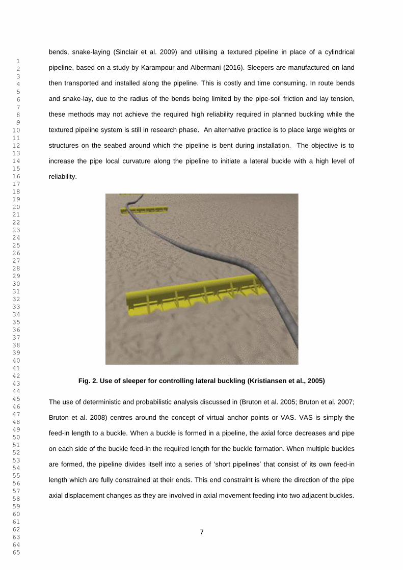
Controlling lateral buckling can be achieved using various methods such as utilizing a subsea

structure that acts as buckle initiator commonly called a sleeper (shown in Fig. 2) , use of route

1 2 3 4 5 6 7 8 9 10 11 12 13 14 15 16 17 18 19 20 21 22 23 24 25 26 27 28 29 30 31 32 33 34 35 36 37 38 39 40 41 42 43 44 45 46 47 48 49 50 51 52 53 54 55 56 57 58 59 60 61 62 63 64 65

7

bends, snake-laying (Sinclair et al. 2009) and utilising a textured pipeline in place of a cylindrical

pipeline, based on a study by Karampour and Albermani (2016). Sleepers are manufactured on land

then transported and installed along the pipeline. This is costly and time consuming. In route bends

and snake-lay, due to the radius of the bends being limited by the pipe-soil friction and lay tension,

these methods may not achieve the required high reliability required in planned buckling while the

textured pipeline system is still in research phase. An alternative practice is to place large weights or

structures on the seabed around which the pipeline is bent during installation. The objective is to

increase the pipe local curvature along the pipeline to initiate a lateral buckle with a high level of

reliability.

Fig. 2. Use of sleeper for controlling lateral buckling (Kristiansen et al., 2005)

The use of deterministic and probabilistic analysis discussed in (Bruton et al. 2005; Bruton et al. 2007;

Bruton et al. 2008) centres around the concept of virtual anchor points or VAS. VAS is simply the

feed-in length to a buckle. When a buckle is formed in a pipeline, the axial force decreases and pipe

on each side of the buckle feed-in the required length for the buckle formation. When multiple buckles

are formed, the pipeline divides itself into a series of ‘short pipelines’ that consist of its own feed-in

length which are fully constrained at their ends. This end constraint is where the direction of the pipe

axial displacement changes as they are involved in axial movement feeding into two adjacent buckles.

1 2 3 4 5 6 7 8 9 10 11 12 13 14 15 16 17 18 19 20 21 22 23 24 25 26 27 28 29 30 31 32 33 34 35 36 37 38 39 40 41 42 43 44 45 46 47 48 49 50 51 52 53 54 55 56 57 58 59 60 61 62 63 64 65

8

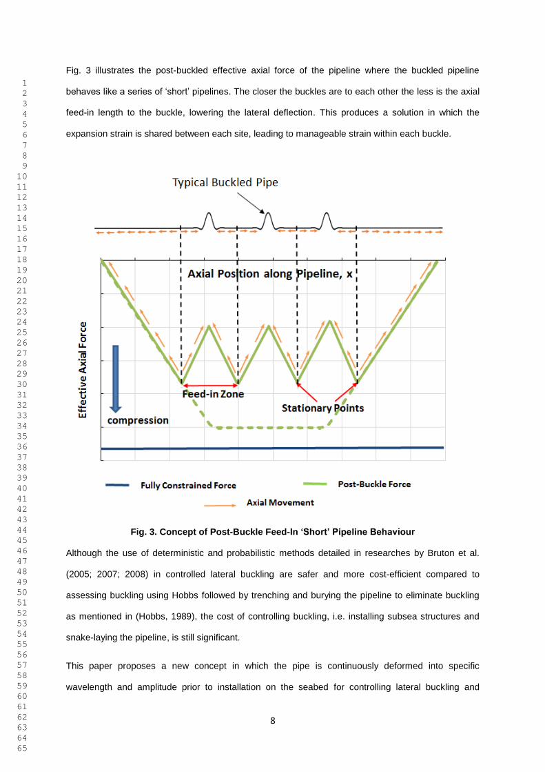
Fig. 3 illustrates the post-buckled effective axial force of the pipeline where the buckled pipeline

behaves like a series of ‘short’ pipelines. The closer the buckles are to each other the less is the axial

feed-in length to the buckle, lowering the lateral deflection. This produces a solution in which the

expansion strain is shared between each site, leading to manageable strain within each buckle.

Fig. 3. Concept of Post-Buckle Feed-In ‘Short’ Pipeline Behaviour

Although the use of deterministic and probabilistic methods detailed in researches by Bruton et al.

(2005; 2007; 2008) in controlled lateral buckling are safer and more cost-efficient compared to

assessing buckling using Hobbs followed by trenching and burying the pipeline to eliminate buckling

as mentioned in (Hobbs, 1989), the cost of controlling buckling, i.e. installing subsea structures and

snake-laying the pipeline, is still significant.

This paper proposes a new concept in which the pipe is continuously deformed into specific

wavelength and amplitude prior to installation on the seabed for controlling lateral buckling and

1 2 3 4 5 6 7 8 9 10 11 12 13 14 15 16 17 18 19 20 21 22 23 24 25 26 27 28 29 30 31 32 33 34 35 36 37 38 39 40 41 42 43 44 45 46 47 48 49 50 51 52 53 54 55 56 57 58 59 60 61 62 63 64 65

9

eliminating the use of subsea structures. Pre-installation out-of-straightness deformations reduce the

axial stiffness of the pipeline sufficiently to allow the pipelines to operate without the need for subsea

structures for controlling lateral buckling could reduce overall cost of installing pipelines and

structures.

2. Pre-Deformation of Pipeline

A pre-deformed pipeline has been successfully installed for controlling lateral buckling. Endal et al.

(2014) and Endal and Nystrom (2015) published a paper detailing the use of the straightener on the

reel-lay barge during reel-lay installation to create residual curvature at specified sections along the

dual 14/16inch pipeline designed for operating temperature up to 95oC for the Skuld Project before it

was laid on the seabed.

In reel-lay installation, the welding together of pipe sections is carried out onshore and then reeled

onto a large drum. The pipeline is plastically bent during the process of reeling. The pipeline is then

unreeled from the drum and the residual bending strains are removed by a straightener system before

leaving the reel ship and laid on the seabed. The method is patented by Statoil (2002) and takes

advantage of the hydraulically adjustable straightener to bend the pipe at specified section to create

specified levels and variations of residual curvature at specific isolated locations along the pipeline.

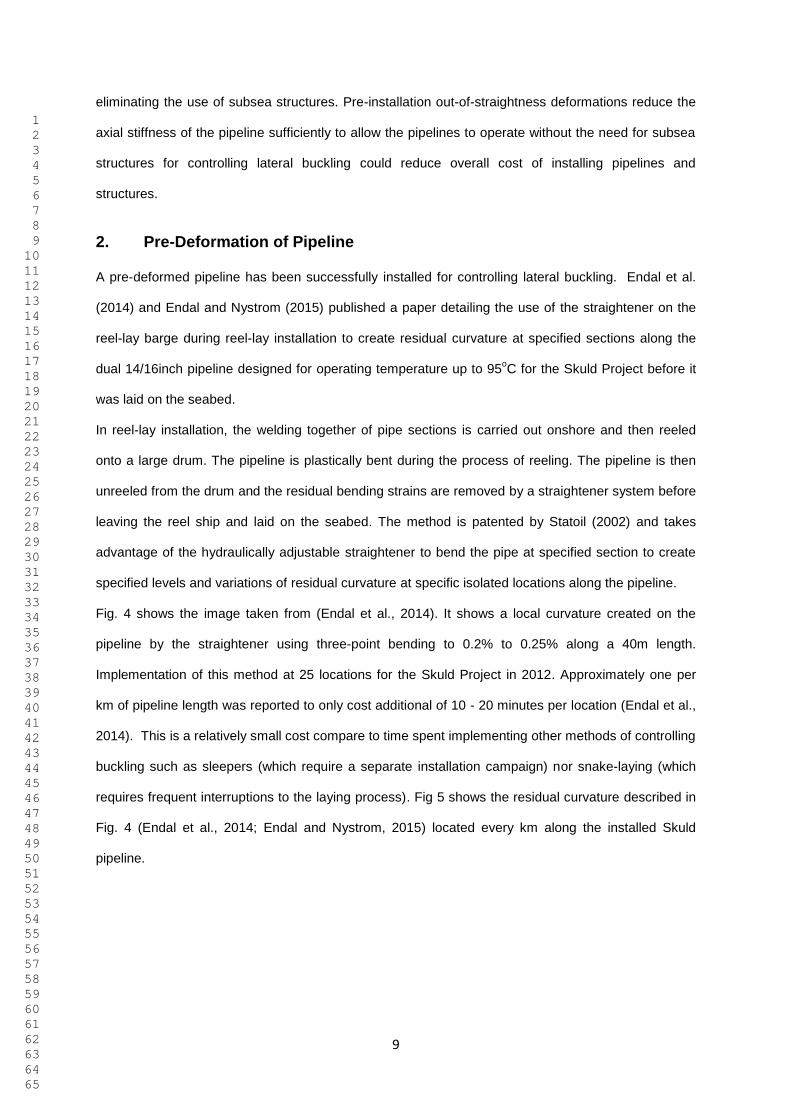
Fig. 4 shows the image taken from (Endal et al., 2014). It shows a local curvature created on the

pipeline by the straightener using three-point bending to 0.2% to 0.25% along a 40m length.

Implementation of this method at 25 locations for the Skuld Project in 2012. Approximately one per

km of pipeline length was reported to only cost additional of 10 - 20 minutes per location (Endal et al.,

2014). This is a relatively small cost compare to time spent implementing other methods of controlling

buckling such as sleepers (which require a separate installation campaign) nor snake-laying (which

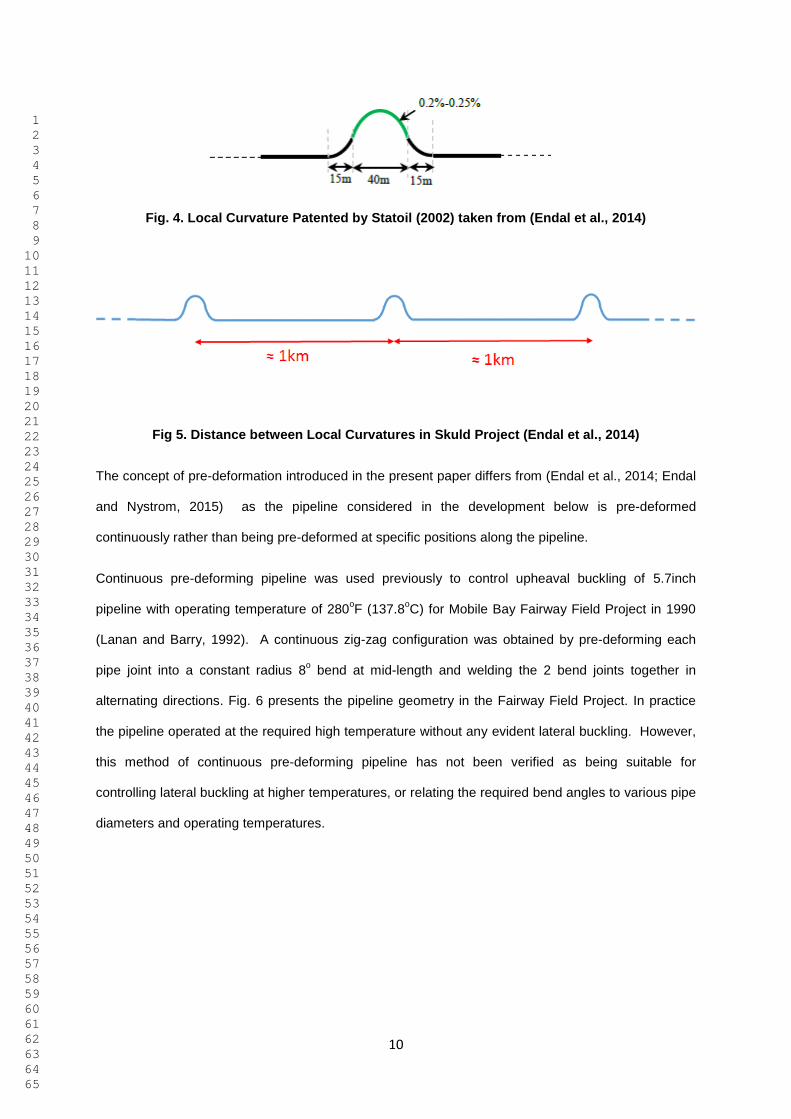
requires frequent interruptions to the laying process). Fig 5 shows the residual curvature described in

Fig. 4 (Endal et al., 2014; Endal and Nystrom, 2015) located every km along the installed Skuld

pipeline.

1 2 3 4 5 6 7 8 9 10 11 12 13 14 15 16 17 18 19 20 21 22 23 24 25 26 27 28 29 30 31 32 33 34 35 36 37 38 39 40 41 42 43 44 45 46 47 48 49 50 51 52 53 54 55 56 57 58 59 60 61 62 63 64 65

10

Fig. 4. Local Curvature Patented by Statoil (2002) taken from (Endal et al., 2014)

Fig 5. Distance between Local Curvatures in Skuld Project (Endal et al., 2014)

The concept of pre-deformation introduced in the present paper differs from (Endal et al., 2014; Endal

and Nystrom, 2015) as the pipeline considered in the development below is pre-deformed

continuously rather than being pre-deformed at specific positions along the pipeline.

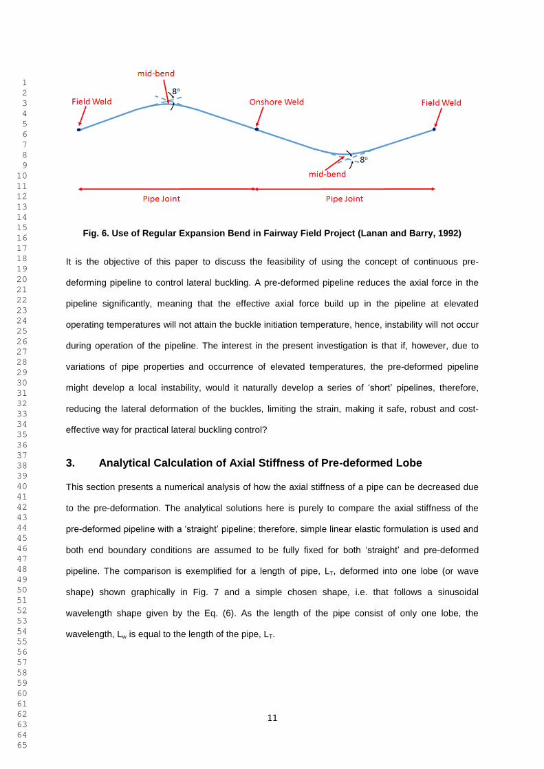
Continuous pre-deforming pipeline was used previously to control upheaval buckling of 5.7inch

pipeline with operating temperature of 280oF (137.8

oC) for Mobile Bay Fairway Field Project in 1990

(Lanan and Barry, 1992). A continuous zig-zag configuration was obtained by pre-deforming each

pipe joint into a constant radius 8o bend at mid-length and welding the 2 bend joints together in

alternating directions. Fig. 6 presents the pipeline geometry in the Fairway Field Project. In practice

the pipeline operated at the required high temperature without any evident lateral buckling. However,

this method of continuous pre-deforming pipeline has not been verified as being suitable for

controlling lateral buckling at higher temperatures, or relating the required bend angles to various pipe

diameters and operating temperatures.

1 2 3 4 5 6 7 8 9 10 11 12 13 14 15 16 17 18 19 20 21 22 23 24 25 26 27 28 29 30 31 32 33 34 35 36 37 38 39 40 41 42 43 44 45 46 47 48 49 50 51 52 53 54 55 56 57 58 59 60 61 62 63 64 65

11

Fig. 6. Use of Regular Expansion Bend in Fairway Field Project (Lanan and Barry, 1992)

It is the objective of this paper to discuss the feasibility of using the concept of continuous pre-

deforming pipeline to control lateral buckling. A pre-deformed pipeline reduces the axial force in the

pipeline significantly, meaning that the effective axial force build up in the pipeline at elevated

operating temperatures will not attain the buckle initiation temperature, hence, instability will not occur

during operation of the pipeline. The interest in the present investigation is that if, however, due to

variations of pipe properties and occurrence of elevated temperatures, the pre-deformed pipeline

might develop a local instability, would it naturally develop a series of ‘short’ pipelines, therefore,

reducing the lateral deformation of the buckles, limiting the strain, making it safe, robust and cost-

effective way for practical lateral buckling control?

3. Analytical Calculation of Axial Stiffness of Pre-deformed Lobe

This section presents a numerical analysis of how the axial stiffness of a pipe can be decreased due

to the pre-deformation. The analytical solutions here is purely to compare the axial stiffness of the

pre-deformed pipeline with a ‘straight’ pipeline; therefore, simple linear elastic formulation is used and

both end boundary conditions are assumed to be fully fixed for both ‘straight’ and pre-deformed

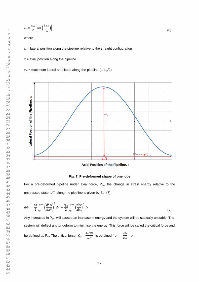
pipeline. The comparison is exemplified for a length of pipe, LT, deformed into one lobe (or wave

shape) shown graphically in Fig. 7 and a simple chosen shape, i.e. that follows a sinusoidal

wavelength shape given by the Eq. (6). As the length of the pipe consist of only one lobe, the

wavelength, Lw is equal to the length of the pipe, LT.

1 2 3 4 5 6 7 8 9 10 11 12 13 14 15 16 17 18 19 20 21 22 23 24 25 26 27 28 29 30 31 32 33 34 35 36 37 38 39 40 41 42 43 44 45 46 47 48 49 50 51 52 53 54 55 56 57 58 59 60 61 62 63 64 65

12

(6)

where

= lateral position along the pipeline relative to the straight configuration

x = axial position along the pipeline

o = maximum lateral amplitude along the pipeline (at Lw/2)

Fig. 7. Pre-deformed shape of one lobe

For a pre-deformed pipeline under axial force, Pax, the change in strain energy relative to the

unstressed state, d along the pipeline is given by Eq. (7):

(7)

Any increased in Pax, will caused an increase in energy and the system will be statically unstable. The

system will deflect and\or deform to minimise the energy. This force will be called the critical force and

be defined as Pcr. The critical force,

, is obtained from

.

1 2 3 4 5 6 7 8 9 10 11 12 13 14 15 16 17 18 19 20 21 22 23 24 25 26 27 28 29 30 31 32 33 34 35 36 37 38 39 40 41 42 43 44 45 46 47 48 49 50 51 52 53 54 55 56 57 58 59 60 61 62 63 64 65

13

As the axial load increases, there is a change of energy of pre-deformed lobe due to a change in

amplitude and shortening of the axial length. Eq. (8) shows the shortening of the axial length, ΔS of

the pipeline feeding into the lateral deflection of the pre-deformed shape is simply:

(8)

The total axial displacement, ΔTot is displacement of the pipe wave without lateral deflection and the

shortening due to lateral deflection. This is shown in Eq. (9).

(9)

Stiffness of the pre-deformed wave, Kp is therefore

and is given by Eq. (10):

(10)

The second term on the denominator controls the fall in axial stiffness of the pre-deformed wave

relative to the straight pipe case, and as 0 0 the solution reverts to a straight pipe. For a specified

wavelength, Lw and amplitude of a lobe, 0, an increased in axial force, Pax causes the stiffness, Kp to

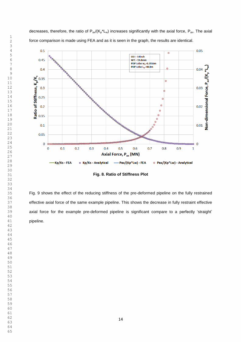
decrease. Fig. 8 presents the calculated ratio of stiffness (stiffness of pre-deformed wave, and since

uniform conditions are considered along the pipeline, the stiffness of the full length of the pipeline

from Eq. (10), Kp divided by the stiffness of straight pipeline, Ks (= EA/LT), for example pipeline with

properties presented in Table 1 against the axial force. At infinitesimal axial force, the axial stiffness of

the pre-deformed pipeline is slightly less than half the stiffness of the straight pipeline. As the applied

axial force is increased, the ratio of stiffness decreases and approaches zero at about 1MN of axial

force for the example case. This is because the stiffness of pre-deformed pipeline reaches a constant

value after 1MN of applied force while the stiffness of the straight pipeline keeps increasing with

applied axial force. Also included in Fig. 8 is the non-dimensional axial force of the pre-deformed

wave, Pax/(Kp*Lw). As the axial force increases, the axial stiffness of the pre-deformed wave

1 2 3 4 5 6 7 8 9 10 11 12 13 14 15 16 17 18 19 20 21 22 23 24 25 26 27 28 29 30 31 32 33 34 35 36 37 38 39 40 41 42 43 44 45 46 47 48 49 50 51 52 53 54 55 56 57 58 59 60 61 62 63 64 65

14

decreases, therefore, the ratio of Pax/(Kp*Lw) increases significantly with the axial force, Pax. The axial

force comparison is made using FEA and as it is seen in the graph, the results are identical.

Fig. 8. Ratio of Stiffness Plot

Fig. 9 shows the effect of the reducing stiffness of the pre-deformed pipeline on the fully restrained

effective axial force of the same example pipeline. This shows the decrease in fully restraint effective

axial force for the example pre-deformed pipeline is significant compare to a perfectly ‘straight’

pipeline.

1 2 3 4 5 6 7 8 9 10 11 12 13 14 15 16 17 18 19 20 21 22 23 24 25 26 27 28 29 30 31 32 33 34 35 36 37 38 39 40 41 42 43 44 45 46 47 48 49 50 51 52 53 54 55 56 57 58 59 60 61 62 63 64 65

15

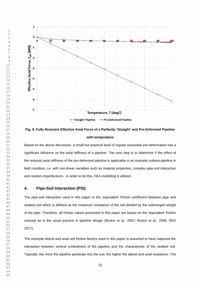
Fig. 9. Fully Restraint Effective Axial Force of a Perfectly ‘Straight’ and Pre-Deformed Pipeline

with temperature

Based on the above discussion, a small but practical level of regular sinusoidal pre-deformation has a

significant influence on the axial stiffness of a pipeline. The next step is to determine if the effect of

the reduced axial stiffness of the pre-deformed pipeline is applicable in an example subsea pipeline in

field condition, i.e. with non-linear variables such as material properties, complex pipe-soil interaction

and random imperfections. In order to do this, FEA modelling is utilized.

4. Pipe-Soil Interaction (PSI)

The pipe-soil interaction used in this paper is the ‘equivalent’ friction coefficient between pipe and

seabed soil which is defined as the maximum resistance of the soil divided by the submerged weight

of the pipe. Therefore, all friction values presented in this paper are based on the ‘equivalent’ friction

concept as is the usual practice in pipeline design (Bruton et al., 2007; Bruton et al., 2008, DNV

2017).

The example lateral and axial soil friction factors used in this paper is assumed to have captured the

interaction between vertical embedment of the pipeline and the characteristic of the seabed soil.

Typically, the more the pipeline penetrate into the soil, the higher the lateral and axial resistance. The

1 2 3 4 5 6 7 8 9 10 11 12 13 14 15 16 17 18 19 20 21 22 23 24 25 26 27 28 29 30 31 32 33 34 35 36 37 38 39 40 41 42 43 44 45 46 47 48 49 50 51 52 53 54 55 56 57 58 59 60 61 62 63 64 65

16

prediction of the axial and lateral resistance of the pipe-soil interaction based on penetration depth

into the seabed soil and its uncertainty can be found in (White and Randolph, 2007). With this

assumption, the coupling between flowline embedment and PSI is not taken into account in the FEA

model in this paper. Therefore, the seabed surface is modelled as a flat, hard surface with very high

vertical stiffness (~106N/m

2).

For all the FE calculations performed, soil modelling is based on uncoupled axial and lateral coulomb

friction. Extensive work had been done to establish the uncoupled behaviour of axial and lateral soil

acting on the pipeline during lateral buckling analysis (Bruton et al., 2007; Bruton et al., 2008; White

and Cheuk, 2008). Separate values are assigned to the axial and lateral equivalent friction factors,

hence, the failure surface which determines when sliding occurs is rectangular (see Fig. 10). This

results in axial and lateral friction behaviours that are independent of each other.

Fig. 10. Failure Surface for PSI

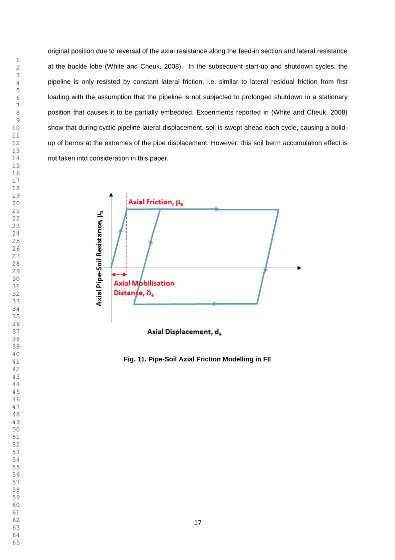
A simple bi-linear axial response of a pipeline on the seabed is assumed in this paper and is shown in

Fig. 11. This assumption is applicable for pipeline with axial displacement that occurs slowly, with no

excess pore pressure generation. Potential changes in axial friction due to consolidation effects

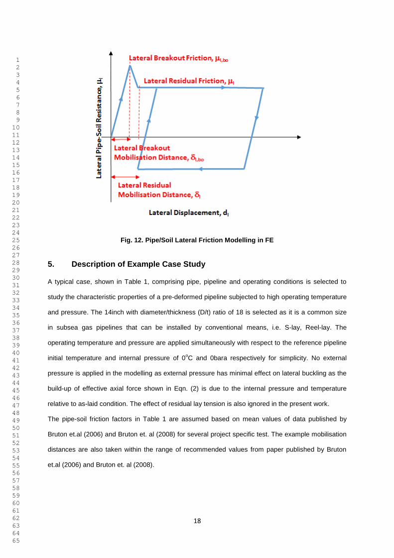
between episodes of movement are ignored for simplicity. Fig. 12 shows the lateral response of a

pipeline on the seabed. Due to as-laid embedment of the pipeline, during the first loading, the partially

embedded pipeline undergoing lateral movement, needs to ‘break-out’ and rises as it moves laterally,

mobilising an initial peak in resistance. The lateral resistance for break-out is usually high. The lateral

resistance then reduces to a steady residual resistance (White and Cheuk, 2008). Therefore, the PSI

response for the first start-up is a tri-linear behaviour. During the first shutdown, the pipeline displaces

in a reverse direction compared to start-up. However, the pipeline does not displace back to its

1 2 3 4 5 6 7 8 9 10 11 12 13 14 15 16 17 18 19 20 21 22 23 24 25 26 27 28 29 30 31 32 33 34 35 36 37 38 39 40 41 42 43 44 45 46 47 48 49 50 51 52 53 54 55 56 57 58 59 60 61 62 63 64 65

17

original position due to reversal of the axial resistance along the feed-in section and lateral resistance

at the buckle lobe (White and Cheuk, 2008). In the subsequent start-up and shutdown cycles, the

pipeline is only resisted by constant lateral friction, i.e. similar to lateral residual friction from first

loading with the assumption that the pipeline is not subjected to prolonged shutdown in a stationary

position that causes it to be partially embedded. Experiments reported in (White and Cheuk, 2008)

show that during cyclic pipeline lateral displacement, soil is swept ahead each cycle, causing a build-

up of berms at the extremes of the pipe displacement. However, this soil berm accumulation effect is

not taken into consideration in this paper.

Fig. 11. Pipe-Soil Axial Friction Modelling in FE

1 2 3 4 5 6 7 8 9 10 11 12 13 14 15 16 17 18 19 20 21 22 23 24 25 26 27 28 29 30 31 32 33 34 35 36 37 38 39 40 41 42 43 44 45 46 47 48 49 50 51 52 53 54 55 56 57 58 59 60 61 62 63 64 65

18

Fig. 12. Pipe/Soil Lateral Friction Modelling in FE

5. Description of Example Case Study

A typical case, shown in Table 1, comprising pipe, pipeline and operating conditions is selected to

study the characteristic properties of a pre-deformed pipeline subjected to high operating temperature

and pressure. The 14inch with diameter/thickness (D/t) ratio of 18 is selected as it is a common size

in subsea gas pipelines that can be installed by conventional means, i.e. S-lay, Reel-lay. The

operating temperature and pressure are applied simultaneously with respect to the reference pipeline

initial temperature and internal pressure of 0oC and 0bara respectively for simplicity. No external

pressure is applied in the modelling as external pressure has minimal effect on lateral buckling as the

build-up of effective axial force shown in Eqn. (2) is due to the internal pressure and temperature

relative to as-laid condition. The effect of residual lay tension is also ignored in the present work.

The pipe-soil friction factors in Table 1 are assumed based on mean values of data published by

Bruton et.al (2006) and Bruton et. al (2008) for several project specific test. The example mobilisation

distances are also taken within the range of recommended values from paper published by Bruton

et.al (2006) and Bruton et. al (2008).

1 2 3 4 5 6 7 8 9 10 11 12 13 14 15 16 17 18 19 20 21 22 23 24 25 26 27 28 29 30 31 32 33 34 35 36 37 38 39 40 41 42 43 44 45 46 47 48 49 50 51 52 53 54 55 56 57 58 59 60 61 62 63 64 65

19

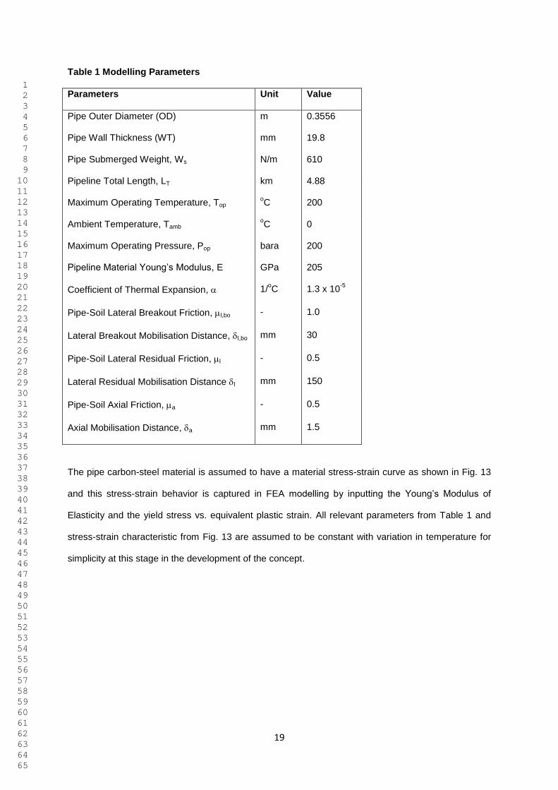
Table 1 Modelling Parameters

Parameters Unit Value

Pipe Outer Diameter (OD) m 0.3556

Pipe Wall Thickness (WT) mm 19.8

Pipe Submerged Weight, Ws N/m 610

Pipeline Total Length, LT km 4.88

Maximum Operating Temperature, Top oC 200

Ambient Temperature, Tamb oC 0

Maximum Operating Pressure, Pop bara 200

Pipeline Material Young’s Modulus, E GPa 205

Coefficient of Thermal Expansion, 1/oC 1.3 x 10

-5

Pipe-Soil Lateral Breakout Friction, l,bo - 1.0

Lateral Breakout Mobilisation Distance, l,bo mm 30

Pipe-Soil Lateral Residual Friction, l - 0.5

Lateral Residual Mobilisation Distance l mm 150

Pipe-Soil Axial Friction, a - 0.5

Axial Mobilisation Distance, a mm 1.5

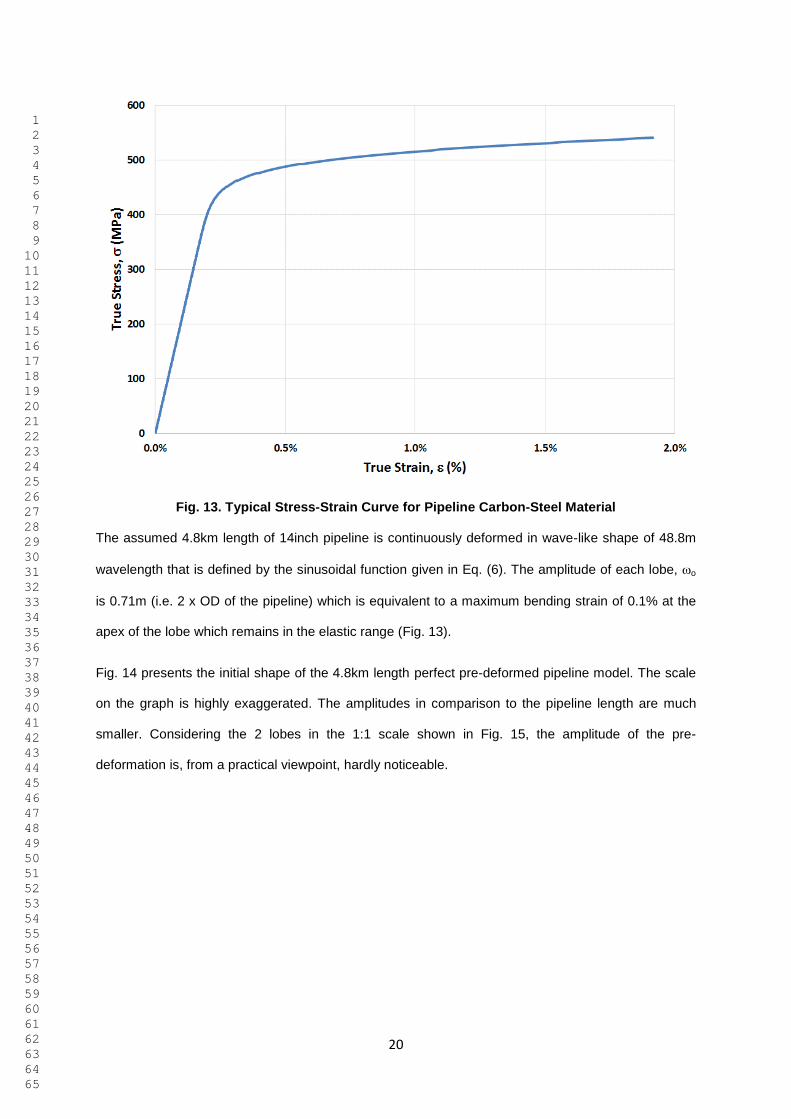
The pipe carbon-steel material is assumed to have a material stress-strain curve as shown in Fig. 13

and this stress-strain behavior is captured in FEA modelling by inputting the Young’s Modulus of

Elasticity and the yield stress vs. equivalent plastic strain. All relevant parameters from Table 1 and

stress-strain characteristic from Fig. 13 are assumed to be constant with variation in temperature for

simplicity at this stage in the development of the concept.

1 2 3 4 5 6 7 8 9 10 11 12 13 14 15 16 17 18 19 20 21 22 23 24 25 26 27 28 29 30 31 32 33 34 35 36 37 38 39 40 41 42 43 44 45 46 47 48 49 50 51 52 53 54 55 56 57 58 59 60 61 62 63 64 65

20

Fig. 13. Typical Stress-Strain Curve for Pipeline Carbon-Steel Material

The assumed 4.8km length of 14inch pipeline is continuously deformed in wave-like shape of 48.8m

wavelength that is defined by the sinusoidal function given in Eq. (6). The amplitude of each lobe, o

is 0.71m (i.e. 2 x OD of the pipeline) which is equivalent to a maximum bending strain of 0.1% at the

apex of the lobe which remains in the elastic range (Fig. 13).

Fig. 14 presents the initial shape of the 4.8km length perfect pre-deformed pipeline model. The scale

on the graph is highly exaggerated. The amplitudes in comparison to the pipeline length are much

smaller. Considering the 2 lobes in the 1:1 scale shown in Fig. 15, the amplitude of the pre-

deformation is, from a practical viewpoint, hardly noticeable.

1 2 3 4 5 6 7 8 9 10 11 12 13 14 15 16 17 18 19 20 21 22 23 24 25 26 27 28 29 30 31 32 33 34 35 36 37 38 39 40 41 42 43 44 45 46 47 48 49 50 51 52 53 54 55 56 57 58 59 60 61 62 63 64 65

21

Fig. 14. Initial Shape of Perfect Pre-deformed pipeline

Fig. 15. Initial Shape of Perfect Pre-deformed pipeline (two lobes in 1:1 scale)

1 2 3 4 5 6 7 8 9 10 11 12 13 14 15 16 17 18 19 20 21 22 23 24 25 26 27 28 29 30 31 32 33 34 35 36 37 38 39 40 41 42 43 44 45 46 47 48 49 50 51 52 53 54 55 56 57 58 59 60 61 62 63 64 65

22

At both ends of the pipeline, two spring elements, one acting along the pipeline axial direction and

one acting on the pipeline lateral direction are modelled with a linear elastic stiffness of 100kN/m to

represent a typical practical stiffness of end expansion spools.

6. Finite Element Analysis (FEA) Modelling

Finite Element software ABAQUS 6.14 (Abaqus, 2014) is used to model the example of a pre-

deformed pipe on the seabed. The FEA modelling exemplified in this section is intended to show the

advantage of using a pre-deformed pipeline in controlling lateral buckling.

6.1 Pipe Elements

The pipe elements used for modelling the flowline in ABAQUS 6.14 are PIPE31H (Abaqus, 2014).

This pipe element from ABAQUS is 3D two node linear pipe element with 6 DOF at each node and

numerical integration of material response at 32 integration points around the circumference.

PIPE31H uses Timoshenko beam formulation that allowed transverse shear deformation. ‘H’ at the

end of the element name in ABAQUS defines hybrid formulation. Hybrid beam elements are used to

improve numerical convergence of beam where the axial stiffness of the beam is much larger

compared to the bending stiffness (Abaqus, 2014). This is useful especially in lateral buckling analysis

of where axially rigid long beam or pipeline undergoes large rotation when it buckles.

6.2 PSI and Seabed Model ling

In all the example FEA calculations, the seabed is modelled as a flat horizontal rigid surface. Contact

pairs are used to model the interaction between the flowline and the seabed surface. ABAQUS user

subroutine FRIC (Abaqus, 2014) is used to capture the effect of independent axial and lateral

components of the contact surface. The subroutine is also necessary to account for a tri-linear lateral

resistance behaviour for the pipeline first start-up. Both axial and lateral resistance are also assumed

to be independent of vertical penetration of the slave surface, i.e. the pipe element into the master

surface, i.e. rigid surface. Therefore, an increase in embedment does not result in higher friction

values.

1 2 3 4 5 6 7 8 9 10 11 12 13 14 15 16 17 18 19 20 21 22 23 24 25 26 27 28 29 30 31 32 33 34 35 36 37 38 39 40 41 42 43 44 45 46 47 48 49 50 51 52 53 54 55 56 57 58 59 60 61 62 63 64 65

23

6.3 Loading

The submerged weight of the pipeline is simulated by applying a uniform distributed weight on the

pipe element. No external pressure is applied. Initial temperature is assumed to be 0oC. Internal

pressure of the pipeline prior to operating is assumed to be 0bara. Operating temperature and

pressure are simultaneously applied in constant increments.

7. Results and Discussion

7.1 Perfect Init ial Sinusoidal Pre-Deformation

In this analysis case, the initial as-laid pre-deformed pipeline (PDP) has no variation in the imposed

out-of-straightness, which comprises of identical equally-sized sinusoidal lobes. Each of the lobes are

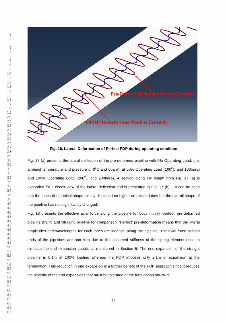
uniform in shape as shown in Fig. 14 and Fig. 16. Fig. 16 taken from ABAQUS presents the detailed

view of the initial shape of the perfect pre-deformed pipeline (blue lines) and after application of

operating temperature and pressure (red lines) respectively. It can be seen in Fig. 16 that the

amplitude of each lobe increases and the pipe displaces laterally to maintain its initial sinusoidal

shape. Maximum displacements at each lobe are not uniform but there is no localization of

deformation of a single lobe (i.e. feed-in of deformation into one or a few lobes caused by structural

instability).

1 2 3 4 5 6 7 8 9 10 11 12 13 14 15 16 17 18 19 20 21 22 23 24 25 26 27 28 29 30 31 32 33 34 35 36 37 38 39 40 41 42 43 44 45 46 47 48 49 50 51 52 53 54 55 56 57 58 59 60 61 62 63 64 65

24

Fig. 16. Lateral Deformation of Perfect PDP during operating condition

Fig. 17 (a) presents the lateral deflection of the pre-deformed pipeline with 0% Operating Load, (i.e.

ambient temperature and pressure of 0oC and 0bara), at 50% Operating Load (100

oC and 100bara)

and 100% Operating Load (200oC and 200bara). A section along the length from Fig. 17 (a) is

expanded for a closer view of the lateral deflection and is presented in Fig. 17 (b). It can be seen

that the lobes of the initial shape simply displace into higher amplitude lobes but the overall shape of

the pipeline has not significantly changed.

Fig. 18 presents the effective axial force along the pipeline for both initially ‘perfect’ pre-deformed

pipeline (PDP) and ‘straight’ pipeline for comparison. ‘Perfect’ pre-deformation means that the lateral

amplitudes and wavelengths for each lobes are identical along the pipeline. The axial force at both

ends of the pipelines are non-zero due to the assumed stiffness of the spring element used to

simulate the end expansion spools as mentioned in Section 5. The end expansion of the straight

pipeline is 6.1m at 100% loading whereas the PDP imposes only 2.1m of expansion at the

termination. This reduction in end expansion is a further benefit of the PDP approach since it reduces

the severity of the end expansions that must be tolerated at the termination structure

1 2 3 4 5 6 7 8 9 10 11 12 13 14 15 16 17 18 19 20 21 22 23 24 25 26 27 28 29 30 31 32 33 34 35 36 37 38 39 40 41 42 43 44 45 46 47 48 49 50 51 52 53 54 55 56 57 58 59 60 61 62 63 64 65

25

It can be seen that the maximum effective axial force of the ‘straight’ pipeline is more than double that

of the PDP. This is because the axial stiffness of the PDP is so much lower than the ‘straight’ pipeline.

Another significant difference is that the effective axial force profile for the perfect ‘straight’ pipeline

behaves as a ‘short pipeline’ where the fully constrained effective force is not attained while the PDP

behaves as a ‘long pipeline’ where it reaches the fully restrained force which is much lower compared

to fully restrained effective force of the ‘straight’ pipeline (as shown in Fig. 9).

No changes in mode shape of the lobes or effective axial force profile of the pre-deformed pipeline

occur. This is confirmed by Fig. 19, which is the plot of effective axial force against the percentage of

operational loading taken at mid length of the PDP and the perfectly ‘straight’ pipeline. It can be seen

that the effective axial force for both PDP and perfectly ‘straight’ pipeline in Fig. 19 keeps increasing

with temperature and pressure loading with no drop in the axial force as no mode changes occur in

both the pipelines. However, the effective axial force of the ‘straight’ pipeline increases linearly with

operating load while the rate of change of effective force for PDP is decreasing with operating load.

The change of slope of the axial force against operating load for the straight pipeline that occurs at

about 15% of the operating load is due to the pipeline changing from being a ‘long pipeline’ with fully

restrained section to ‘short pipeline’ with only partially restrained section. This is because at about

15% operating load, the axial resistance of the soil is no longer able to resist the axial expansion of

the pipeline.

1 2 3 4 5 6 7 8 9 10 11 12 13 14 15 16 17 18 19 20 21 22 23 24 25 26 27 28 29 30 31 32 33 34 35 36 37 38 39 40 41 42 43 44 45 46 47 48 49 50 51 52 53 54 55 56 57 58 59 60 61 62 63 64 65

26

(a)

(b)

Fig. 17. Lateral Deflection for Perfect Pre-Deformed Pipeline

1 2 3 4 5 6 7 8 9 10 11 12 13 14 15 16 17 18 19 20 21 22 23 24 25 26 27 28 29 30 31 32 33 34 35 36 37 38 39 40 41 42 43 44 45 46 47 48 49 50 51 52 53 54 55 56 57 58 59 60 61 62 63 64 65

27

Fig. 18. Effective Axial Force for Perfect Pre-Deformed and ‘Straight’ Pipeline

Fig. 19. Variation of Effective Axial Force with Operating Load at mid length of Perfect Pre-

Deformed and ‘Straight’ Pipeline

1 2 3 4 5 6 7 8 9 10 11 12 13 14 15 16 17 18 19 20 21 22 23 24 25 26 27 28 29 30 31 32 33 34 35 36 37 38 39 40 41 42 43 44 45 46 47 48 49 50 51 52 53 54 55 56 57 58 59 60 61 62 63 64 65

28

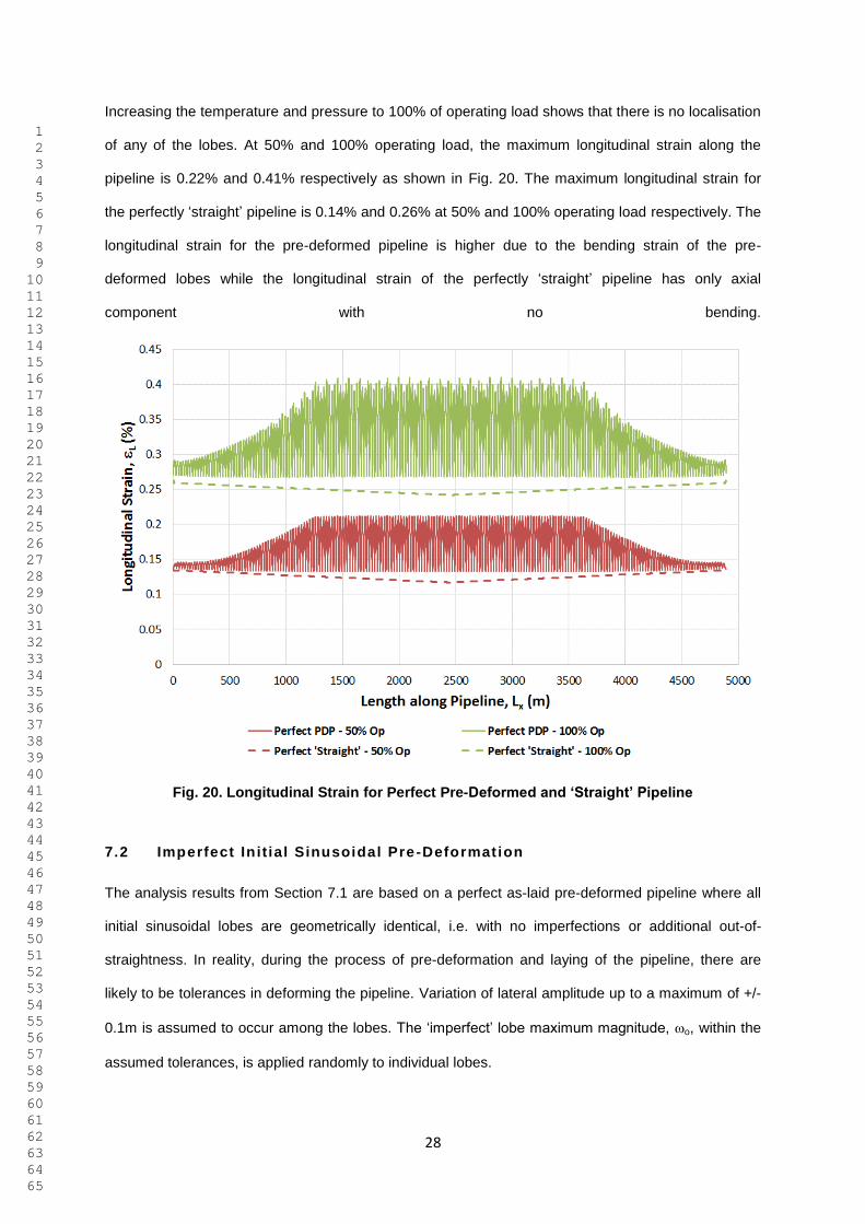
Increasing the temperature and pressure to 100% of operating load shows that there is no localisation

of any of the lobes. At 50% and 100% operating load, the maximum longitudinal strain along the

pipeline is 0.22% and 0.41% respectively as shown in Fig. 20. The maximum longitudinal strain for

the perfectly ‘straight’ pipeline is 0.14% and 0.26% at 50% and 100% operating load respectively. The

longitudinal strain for the pre-deformed pipeline is higher due to the bending strain of the pre-

deformed lobes while the longitudinal strain of the perfectly ‘straight’ pipeline has only axial

component with no bending.

Fig. 20. Longitudinal Strain for Perfect Pre-Deformed and ‘Straight’ Pipeline

7.2 Imperfect Init ial Sinusoidal Pre -Deformation

The analysis results from Section 7.1 are based on a perfect as-laid pre-deformed pipeline where all

initial sinusoidal lobes are geometrically identical, i.e. with no imperfections or additional out-of-

straightness. In reality, during the process of pre-deformation and laying of the pipeline, there are

likely to be tolerances in deforming the pipeline. Variation of lateral amplitude up to a maximum of +/-

0.1m is assumed to occur among the lobes. The ‘imperfect’ lobe maximum magnitude, o, within the

assumed tolerances, is applied randomly to individual lobes.

1 2 3 4 5 6 7 8 9 10 11 12 13 14 15 16 17 18 19 20 21 22 23 24 25 26 27 28 29 30 31 32 33 34 35 36 37 38 39 40 41 42 43 44 45 46 47 48 49 50 51 52 53 54 55 56 57 58 59 60 61 62 63 64 65

29

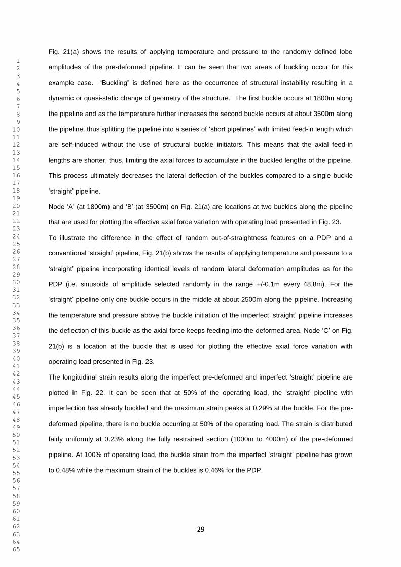
Fig. 21(a) shows the results of applying temperature and pressure to the randomly defined lobe

amplitudes of the pre-deformed pipeline. It can be seen that two areas of buckling occur for this

example case. “Buckling” is defined here as the occurrence of structural instability resulting in a

dynamic or quasi-static change of geometry of the structure. The first buckle occurs at 1800m along

the pipeline and as the temperature further increases the second buckle occurs at about 3500m along

the pipeline, thus splitting the pipeline into a series of ‘short pipelines’ with limited feed-in length which

are self-induced without the use of structural buckle initiators. This means that the axial feed-in

lengths are shorter, thus, limiting the axial forces to accumulate in the buckled lengths of the pipeline.

This process ultimately decreases the lateral deflection of the buckles compared to a single buckle

‘straight’ pipeline.

Node ‘A’ (at 1800m) and ‘B’ (at 3500m) on Fig. 21(a) are locations at two buckles along the pipeline

that are used for plotting the effective axial force variation with operating load presented in Fig. 23.

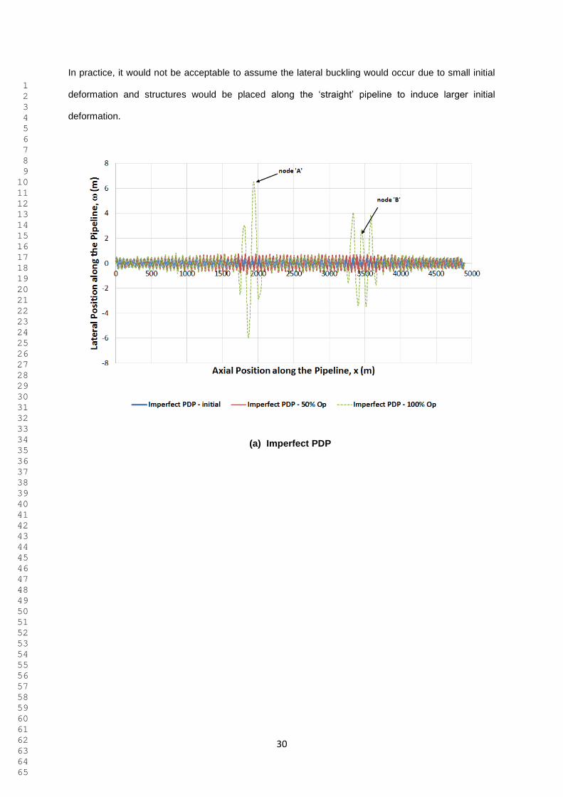
To illustrate the difference in the effect of random out-of-straightness features on a PDP and a

conventional ‘straight’ pipeline, Fig. 21(b) shows the results of applying temperature and pressure to a

‘straight’ pipeline incorporating identical levels of random lateral deformation amplitudes as for the

PDP (i.e. sinusoids of amplitude selected randomly in the range +/-0.1m every 48.8m). For the

‘straight’ pipeline only one buckle occurs in the middle at about 2500m along the pipeline. Increasing

the temperature and pressure above the buckle initiation of the imperfect ‘straight’ pipeline increases

the deflection of this buckle as the axial force keeps feeding into the deformed area. Node ‘C’ on Fig.

21(b) is a location at the buckle that is used for plotting the effective axial force variation with

operating load presented in Fig. 23.

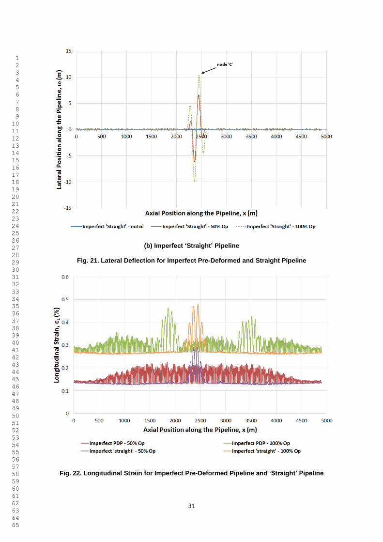
The longitudinal strain results along the imperfect pre-deformed and imperfect ‘straight’ pipeline are

plotted in Fig. 22. It can be seen that at 50% of the operating load, the ‘straight’ pipeline with

imperfection has already buckled and the maximum strain peaks at 0.29% at the buckle. For the pre-

deformed pipeline, there is no buckle occurring at 50% of the operating load. The strain is distributed

fairly uniformly at 0.23% along the fully restrained section (1000m to 4000m) of the pre-deformed

pipeline. At 100% of operating load, the buckle strain from the imperfect ‘straight’ pipeline has grown

to 0.48% while the maximum strain of the buckles is 0.46% for the PDP.

1 2 3 4 5 6 7 8 9 10 11 12 13 14 15 16 17 18 19 20 21 22 23 24 25 26 27 28 29 30 31 32 33 34 35 36 37 38 39 40 41 42 43 44 45 46 47 48 49 50 51 52 53 54 55 56 57 58 59 60 61 62 63 64 65

30

In practice, it would not be acceptable to assume the lateral buckling would occur due to small initial

deformation and structures would be placed along the ‘straight’ pipeline to induce larger initial

deformation.

(a) Imperfect PDP

1 2 3 4 5 6 7 8 9 10 11 12 13 14 15 16 17 18 19 20 21 22 23 24 25 26 27 28 29 30 31 32 33 34 35 36 37 38 39 40 41 42 43 44 45 46 47 48 49 50 51 52 53 54 55 56 57 58 59 60 61 62 63 64 65

31

(b) Imperfect ‘Straight’ Pipeline

Fig. 21. Lateral Deflection for Imperfect Pre-Deformed and Straight Pipeline

Fig. 22. Longitudinal Strain for Imperfect Pre-Deformed Pipeline and ‘Straight’ Pipeline

1 2 3 4 5 6 7 8 9 10 11 12 13 14 15 16 17 18 19 20 21 22 23 24 25 26 27 28 29 30 31 32 33 34 35 36 37 38 39 40 41 42 43 44 45 46 47 48 49 50 51 52 53 54 55 56 57 58 59 60 61 62 63 64 65

32

The physics of buckling along the pipelines is evidently controlled by the temperature (and pressure)

at which buckling occurs. In order to determine the buckle initiation forces, and the stability conditions

at various values of operating load, the effective axial force of the pre-deformed pipeline is plotted

against the operating loads and is shown in Fig. 23. The locations where the effective axial force

variation is taken is at Node ‘A’ and ‘B’ for PDP on Fig. 21(a) and Node ‘C’ on Fig. 21(b). These

represent the nodes at which the maximum deflection and longitudinal strain occur. Also plotted in

Fig. 23 are the effective axial force variations for perfect PDP and ‘straight’ pipe from Fig. 19.

It can be seen in Fig. 23 that the FEA modelling of a ‘straight’ pipeline with random imposed

imperfection has a sudden drop of effective axial force consistent with the occurrence of a buckle at

16.2% of the operating load, which is 32.3oC (with corresponding pressure of 32.3bara). For the pre-

deformed pipeline, tracing the effective axial force with increasing operating load at Node ‘A’ shows

that the pre-deformed pipeline with random imperfections first buckles at this location (approximately

1800m along pipeline) at 74.8% operating load, which is 149.6oC (with corresponding pressure of

149.6bara). A second buckle was formed at Node ‘B’ (approximately 3500m along pipeline) and

tracing the effective axial force variation at this location shows the buckle initiates at about 83.0% of

the operating load, or 166.0oC (with the corresponding pressure of 166.0bara).

This is a significant increase in the operating loads at which onset of buckling occurs for the imperfect

PDP compared to the ‘straight’ pipeline with random imperfection. This means that if this example

pipeline with the specified out-of-straightness in the pre-deformed shape, is operating at differential

temperature of 149.6oC and below, unplanned lateral buckling is very unlikely to occur. Assuming the

average ambient temperature of 20oC, the operating temperature of the pipeline has to be about

170oC to initiate a buckle if the method of pre-deformation is used in controlling lateral buckling with

the assumed levels for random ‘imperfections’.

Another notable point that is that the use of Hobbs analytical method from Eq. (1) predicts lateral

buckling for an initially perfect ‘straight’ pipeline to initiate at 6.0% of the operating load, i.e. about

12oC and 12bara. This shows that using Hobbs for calculation of lateral buckling is extremely

conservative for this example case. A much higher temperature can be applied before buckling

occurs.

1 2 3 4 5 6 7 8 9 10 11 12 13 14 15 16 17 18 19 20 21 22 23 24 25 26 27 28 29 30 31 32 33 34 35 36 37 38 39 40 41 42 43 44 45 46 47 48 49 50 51 52 53 54 55 56 57 58 59 60 61 62 63 64 65

33

Fig. 23. Effective Axial Force vs Operating Load

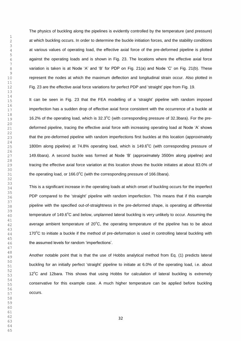
Fig. 24 presents the changes in the effective axial force profile along the pre-deformed pipeline as the

pipeline buckles when subjected to various increments of the operating load. Fig. 24 shows the

effective axial force profile reaching about -0.55MN of fully restrained effective axial force between

1200m and 3800m prior to buckling at about 74.8% of operating load (i.e. 149.6oC and 149.6bara).

Increasing the temperature and pressure slightly to 74.8% operating load initiates a buckle at 1800m

and it can be seen that the effective axial force at that location drops significantly to -0.38MN.

Increasing the temperature and pressure further to 83.0% operating load as shown in Fig. 24 shows

that the effective axial force at buckle location, i.e. 1800m, is significantly reduced to about -0.17MN.

A slight increase of operating load to 83.0% cause another buckle occur to at 3500m. At the end of

the analysis, at applied temperature of 200oC, as shown in Fig. 24, the effective axial force profile

consists of two effectively ‘short pipeline’ sections. The feed-in length of the buckle at 1800m is about

1880m and the feed-in length of the buckle at 3500m is 1500m.

1 2 3 4 5 6 7 8 9 10 11 12 13 14 15 16 17 18 19 20 21 22 23 24 25 26 27 28 29 30 31 32 33 34 35 36 37 38 39 40 41 42 43 44 45 46 47 48 49 50 51 52 53 54 55 56 57 58 59 60 61 62 63 64 65

34

Fig. 24. Effective Axial Force Profile along Imperfect Pre-Deformed Pipeline

Fig. 25 shows how the effective axial force profile for the ‘straight’ pipeline with random imperfections

behaves. The pre-buckle effective axial force for the ‘straight’ pipeline behaves as a ‘short pipeline’

where the drop of effective axial force occurs at about 16.3% operating load which is equivalent to

32.3oC and 32.3bara and as the temperature is increased to 100% operating load, the effective axial

force keeps decreasing as the buckle develops. Feed-in length to the buckle at 200oC is 3180m.

1 2 3 4 5 6 7 8 9 10 11 12 13 14 15 16 17 18 19 20 21 22 23 24 25 26 27 28 29 30 31 32 33 34 35 36 37 38 39 40 41 42 43 44 45 46 47 48 49 50 51 52 53 54 55 56 57 58 59 60 61 62 63 64 65

35

Fig. 25. Effective Axial Force Profile along Imperfect ‘Straight’ Pipeline

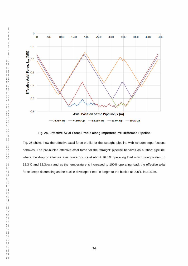
Fig. 26 presents the strain energy plot against the operating load. From the energy point of view, the

system of pre-deformed pipeline tries to attain a lower energy state twice. The first initiation of

instability located at 1800m occurs at 74.8% operating load, i.e. 149.6oC and 149.6bara. As the

temperature and pressure increases, the second instability occurs at 83% operating load. This is

shown by the two step changes in the curve as the temperature increased. In comparison with the

strain energy of a ‘straight’ pipeline that laterally buckled, step change in strain energy during

instability initiation is much more pronounced. For a ‘straight’ pipeline at 16.2% operating load, a

lateral buckle initiates at the mid-length of the pipeline. The reduction in strain energy is almost

negligible because all the axial expansion deformation is fed into a single buckle.

1 2 3 4 5 6 7 8 9 10 11 12 13 14 15 16 17 18 19 20 21 22 23 24 25 26 27 28 29 30 31 32 33 34 35 36 37 38 39 40 41 42 43 44 45 46 47 48 49 50 51 52 53 54 55 56 57 58 59 60 61 62 63 64 65

36

Fig. 26. Strain Energy vs. Operating Load for Imperfect Pre-Deformed Pipeline and ‘Straight’

Pipeline

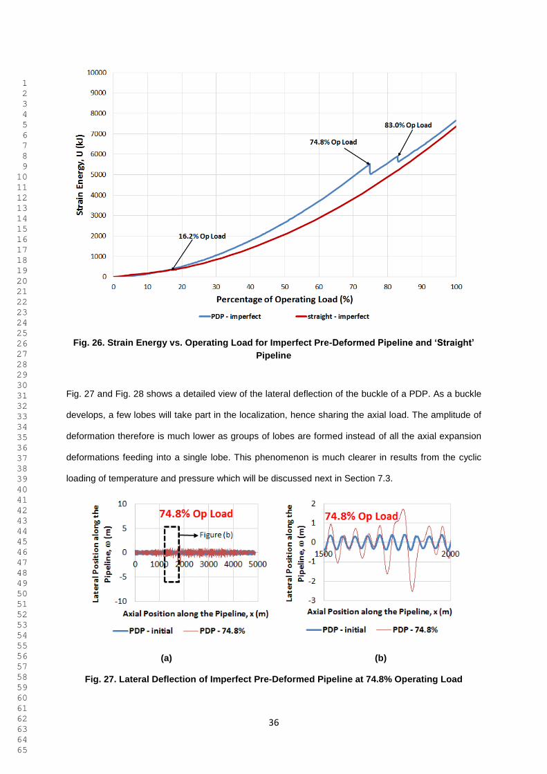
Fig. 27 and Fig. 28 shows a detailed view of the lateral deflection of the buckle of a PDP. As a buckle

develops, a few lobes will take part in the localization, hence sharing the axial load. The amplitude of

deformation therefore is much lower as groups of lobes are formed instead of all the axial expansion

deformations feeding into a single lobe. This phenomenon is much clearer in results from the cyclic

loading of temperature and pressure which will be discussed next in Section 7.3.

(a) (b)

Fig. 27. Lateral Deflection of Imperfect Pre-Deformed Pipeline at 74.8% Operating Load

1 2 3 4 5 6 7 8 9 10 11 12 13 14 15 16 17 18 19 20 21 22 23 24 25 26 27 28 29 30 31 32 33 34 35 36 37 38 39 40 41 42 43 44 45 46 47 48 49 50 51 52 53 54 55 56 57 58 59 60 61 62 63 64 65

37

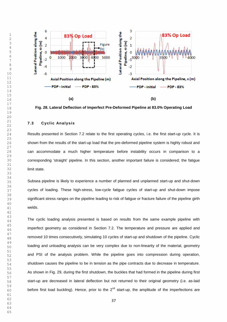
(a) (b)

Fig. 28. Lateral Deflection of Imperfect Pre-Deformed Pipeline at 83.0% Operating Load

7.3 Cycl ic Analysis

Results presented in Section 7.2 relate to the first operating cycles, i.e. the first start-up cycle. It is

shown from the results of the start-up load that the pre-deformed pipeline system is highly robust and

can accommodate a much higher temperature before instability occurs in comparison to a

corresponding ‘straight’ pipeline. In this section, another important failure is considered; the fatigue

limit state.

Subsea pipeline is likely to experience a number of planned and unplanned start-up and shut-down

cycles of loading. These high-stress, low-cycle fatigue cycles of start-up and shut-down impose

significant stress ranges on the pipeline leading to risk of fatigue or fracture failure of the pipeline girth

welds.

The cyclic loading analysis presented is based on results from the same example pipeline with

imperfect geometry as considered in Section 7.2. The temperature and pressure are applied and

removed 10 times consecutively, simulating 10 cycles of start-up and shutdown of the pipeline. Cyclic

loading and unloading analysis can be very complex due to non-linearity of the material, geometry

and PSI of the analysis problem. While the pipeline goes into compression during operation,

shutdown causes the pipeline to be in tension as the pipe contracts due to decrease in temperature.

As shown in Fig. 29, during the first shutdown, the buckles that had formed in the pipeline during first

start-up are decreased in lateral deflection but not returned to their original geometry (i.e. as-laid

before first load buckling). Hence, prior to the 2nd

start-up, the amplitude of the imperfections are

1 2 3 4 5 6 7 8 9 10 11 12 13 14 15 16 17 18 19 20 21 22 23 24 25 26 27 28 29 30 31 32 33 34 35 36 37 38 39 40 41 42 43 44 45 46 47 48 49 50 51 52 53 54 55 56 57 58 59 60 61 62 63 64 65

38

larger than the as-laid condition before the first start-up. This causes the buckle to occur at a lower

force. The lateral deflection is also greater during the 2nd

start-up in comparison to the first start-up.

The lateral deflection gradually grows with the number of start-up operations. Fig. 30 presents the

lateral deformations along the example pipeline during the 1st, 2

nd, 5

th and 10

th start-up. Nodes ‘A’ and

‘B’ are the locations of the plotted variations of lateral deflections and effective axial forces for the pre-

deformed pipeline are shown in Fig. 31 and Fig. 32.

Fig. 29. Lateral Deflection of Imperfect Pre-Deformed Pipeline during the first start-up (SU) and

shutdown (SD)

1 2 3 4 5 6 7 8 9 10 11 12 13 14 15 16 17 18 19 20 21 22 23 24 25 26 27 28 29 30 31 32 33 34 35 36 37 38 39 40 41 42 43 44 45 46 47 48 49 50 51 52 53 54 55 56 57 58 59 60 61 62 63 64 65

39

Fig. 30. Lateral Deflection of Imperfect Pre-Deformed Pipeline during 1st

, 2nd

, 5th

and 10th

Start-

up (SU)

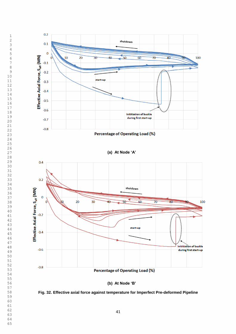
It may be seen that during the first start-up, Fig. 31(a), there is a sudden increase in lateral deflection

at 74.8% Operating Load. Such a sudden increase in lateral deflection corresponding to an extremely

small change in load is called ‘snap buckling’ (Hobbs, 1984) and is a dynamic change of pipeline

geometry. As the amplitude of the imperfection at this location in the pipeline prior to the 2nd

start-up is

much larger than the initial as-laid imperfection, lateral buckling occurs at a much lower operating load

as seen in Fig. 32 (a) and it is even arguable if this should be considered as an example of buckling.

The occurrence of lateral movements is less dramatic without the ‘snap buckling’ effect since there is

no sudden change of axial force. It is simply growth of the initial imperfection with increasing loading

of the pipeline, as reported in (Hobbs, 1984; Nystrom et al., 1997). The increase in lateral deflection

with operating load at Node ‘B’ is shown in Fig. 31(b). Similar to the buckle at location Node ‘A’, the

amplitude of the imperfections after each shutdowns are increased, so that buckling is replaced by a

continuous non-linear increase in lateral deformations due to increasing loading, as shown in Fig.

32(b).

1 2 3 4 5 6 7 8 9 10 11 12 13 14 15 16 17 18 19 20 21 22 23 24 25 26 27 28 29 30 31 32 33 34 35 36 37 38 39 40 41 42 43 44 45 46 47 48 49 50 51 52 53 54 55 56 57 58 59 60 61 62 63 64 65

40

(a) Node ‘A’

(b) Node ‘B’

Fig. 31. Operating Load vs. Lateral Deflection for 1st

, 2nd

, 5th

and 10th

Start-up (SU) for Imperfect

Pre-Deformed Pipeline

1 2 3 4 5 6 7 8 9 10 11 12 13 14 15 16 17 18 19 20 21 22 23 24 25 26 27 28 29 30 31 32 33 34 35 36 37 38 39 40 41 42 43 44 45 46 47 48 49 50 51 52 53 54 55 56 57 58 59 60 61 62 63 64 65

41

(a) At Node ‘A’

(b) At Node ‘B’

Fig. 32. Effective axial force against temperature for Imperfect Pre-deformed Pipeline

1 2 3 4 5 6 7 8 9 10 11 12 13 14 15 16 17 18 19 20 21 22 23 24 25 26 27 28 29 30 31 32 33 34 35 36 37 38 39 40 41 42 43 44 45 46 47 48 49 50 51 52 53 54 55 56 57 58 59 60 61 62 63 64 65

42

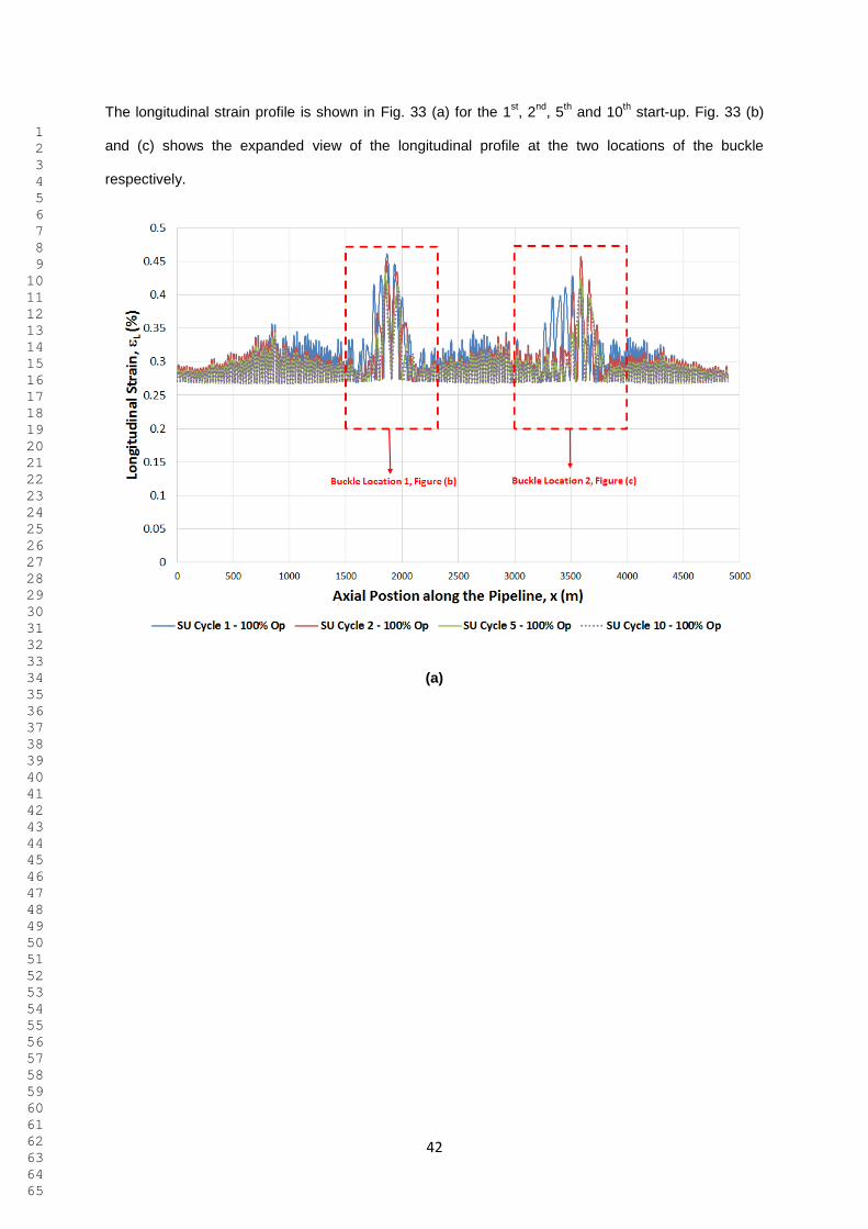
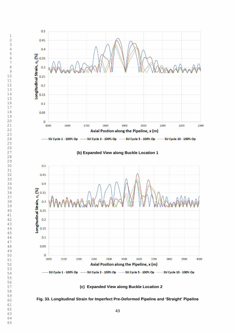
The longitudinal strain profile is shown in Fig. 33 (a) for the 1st, 2

nd, 5

th and 10

th start-up. Fig. 33 (b)

and (c) shows the expanded view of the longitudinal profile at the two locations of the buckle

respectively.

(a)

1 2 3 4 5 6 7 8 9 10 11 12 13 14 15 16 17 18 19 20 21 22 23 24 25 26 27 28 29 30 31 32 33 34 35 36 37 38 39 40 41 42 43 44 45 46 47 48 49 50 51 52 53 54 55 56 57 58 59 60 61 62 63 64 65

43

(b) Expanded View along Buckle Location 1

(c) Expanded View along Buckle Location 2

Fig. 33. Longitudinal Strain for Imperfect Pre-Deformed Pipeline and ‘Straight’ Pipeline

1 2 3 4 5 6 7 8 9 10 11 12 13 14 15 16 17 18 19 20 21 22 23 24 25 26 27 28 29 30 31 32 33 34 35 36 37 38 39 40 41 42 43 44 45 46 47 48 49 50 51 52 53 54 55 56 57 58 59 60 61 62 63 64 65

44

The maximum strain along the PDP always occurs along the buckle location 1 and 2 as shown in Fig.

33 (a) during start-up. As the buckle location varies slightly during each start-up, the maximum

longitudinal strain along the PDP at buckle location 1 from 1500m to 2300m and buckle location 2

from 3000m to 4000m at each start-up cycle is plotted instead of tracing a single point along the

pipeline. This is shown in Fig. 34. The maximum strain of the PDP is highest during first start-up at

0.46%, located at buckle location 1, at maximum operating condition and gradually decreases, due to

a ‘shakedown’ effect within the overall system of PDP lobes, to 0.42% at the end of the 10th start-up.

The ‘shake-down’ of the strain levels along the pipeline reduces the risk of failure by fatigue at girth

welds. This is an important demonstration that the PDP system has a tendency for cyclic strain

ranges in the lobes to stabilise rather than grow.

Fig. 34. Strain vs. Lateral Deflection for Imperfect Pre-Deformed Pipeline during Start-Up

Fig. 35 presents the strain energy against loading cycle for the imperfect pre-deformed pipeline. The

strain energy variation during the first loading cycle is similar to Fig. 26 where the two buckles along

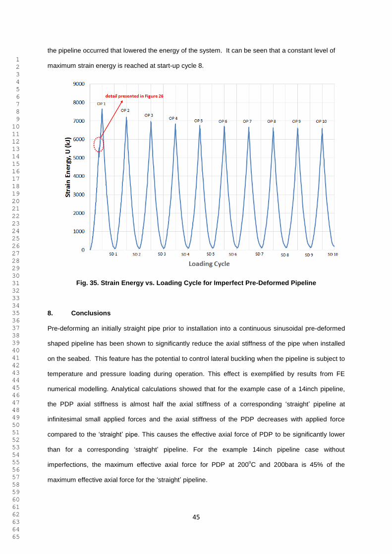
1 2 3 4 5 6 7 8 9 10 11 12 13 14 15 16 17 18 19 20 21 22 23 24 25 26 27 28 29 30 31 32 33 34 35 36 37 38 39 40 41 42 43 44 45 46 47 48 49 50 51 52 53 54 55 56 57 58 59 60 61 62 63 64 65

45

the pipeline occurred that lowered the energy of the system. It can be seen that a constant level of

maximum strain energy is reached at start-up cycle 8.

Fig. 35. Strain Energy vs. Loading Cycle for Imperfect Pre-Deformed Pipeline

8. Conclusions

Pre-deforming an initially straight pipe prior to installation into a continuous sinusoidal pre-deformed

shaped pipeline has been shown to significantly reduce the axial stiffness of the pipe when installed

on the seabed. This feature has the potential to control lateral buckling when the pipeline is subject to

temperature and pressure loading during operation. This effect is exemplified by results from FE

numerical modelling. Analytical calculations showed that for the example case of a 14inch pipeline,

the PDP axial stiffness is almost half the axial stiffness of a corresponding ‘straight’ pipeline at

infinitesimal small applied forces and the axial stiffness of the PDP decreases with applied force

compared to the ‘straight’ pipe. This causes the effective axial force of PDP to be significantly lower

than for a corresponding ‘straight’ pipeline. For the example 14inch pipeline case without

imperfections, the maximum effective axial force for PDP at 200oC and 200bara is 45% of the

maximum effective axial force for the ‘straight’ pipeline.

1 2 3 4 5 6 7 8 9 10 11 12 13 14 15 16 17 18 19 20 21 22 23 24 25 26 27 28 29 30 31 32 33 34 35 36 37 38 39 40 41 42 43 44 45 46 47 48 49 50 51 52 53 54 55 56 57 58 59 60 61 62 63 64 65

46

The primary conclusion drawn from the FEA modelling carried out is that pre-deforming a pipeline in

the manner described here enables the pipeline to accommodate temperatures higher than typical

operating temperature before lateral buckling initiates. With the example PSI properties and example

random imposed out-of-straightness, a PDP pipeline initiates the first buckling only at a differential

temperature, ΔT, of 150oC and differential pressure, ΔP of 150bara while a ‘straight’ pipeline with the

same random out-of-straightness initiates at ΔT of 32oC and ΔP of 32bara. This has significant effect

on the capacity of a pipeline and the practical arrangements needed to deal with thermal expansion.

In fact, delaying the initiation of buckles to a much higher temperature and pressure ensures that such

a pipeline would be very unlikely to buckle in maximum subsea pipeline operating temperatures of

about ΔT of 100oC to 120

oC. Another significant conclusion from the analysis results shown here is

that the PDP initiates another buckle at ΔT of 166oC (with 166bara) at another location. This enables

the formation of two sections of ‘short pipelines’ that limits the feed-in of axial expansions

deformations to the buckled pipe length so that the maximum strain level along the pipeline is not as

high as the ‘straight’ pipeline where the buckle localizes at one location.

This make the pre-deformed pipeline system safer and reliable as a buckle mitigation system. If in an

accidental condition the operating temperature were to increase, say to 150oC compared to the

design level of 120oC, the longitudinal strain of 0.46% during first load would be less than a

corresponding occurrence for the nominally straight pipeline.

This study has shown that the PDP pipeline could be designed to operate at a high level of HPHT

loading without the requirement of special structures installed on the seabed to control the initiation of

lateral buckling and still maintain acceptable levels of axial strains. This feature has very important

consequences for practical pipelines, especially long pipelines in quite deep water for which the

manufacture and installation of the special structures could be very costly and have a deleterious

effect on the schedule of the pipeline system.

Cyclic analysis of the PDP with 10 cycles of start-up and shutdown shows that the application of cyclic

temperature and pressure loading induces a form of shake-down such that the maximum levels of

strain are progressively reduced. This controls and reduces the chance of failure by fatigue.

The results to date show that the concept of pre-deforming a pipeline has potentially significant

advantages for the design, installation and operation of subsea pipeline compared to corresponding

1 2 3 4 5 6 7 8 9 10 11 12 13 14 15 16 17 18 19 20 21 22 23 24 25 26 27 28 29 30 31 32 33 34 35 36 37 38 39 40 41 42 43 44 45 46 47 48 49 50 51 52 53 54 55 56 57 58 59 60 61 62 63 64 65

47

pipeline installed in a nominally straight condition. It could prove to be a valuable tool for the subsea

industry as it enables the pipeline to be installed and operated safely at elevated temperatures without

the need for lateral buckling design and installation of expensive structures as buckle initiators. The

system is shown to be robust and able to adjust itself by geometry rearrangement to minimize the

energy by creating a series of ‘short pipelines’.

The objective of this paper has introduce the concept of PDP in sinusoidal shape for controlling lateral

buckling in comparison with a ‘straight’ pipeline. Further research is underway to determine the effect

of various out-of-straightness geometries and occurrence of random variations of the PSI on the PDP

response of HPHT loading and to investigate the fundamental mechanics governing the buckle

initiation and geometry rearrangement with analytical study. Detail studies have been done to

investigate the behaviour of infinite beams on non-linear foundation by Baek et al. (2014) and Fayyaz

et al. (2017) and the influence of geometric imperfections on pipeline buckling (Gao et al.,

2015).These papers will serve as the basis for the next level of research. Studies are also being made

to determine the optimum shape of pre-deformation to achieve reliability in controlling lateral buckling

and the feasibility installation.

Abbreviations

FEA Finite Modelling Analysis

HPHT High Pressure High Temperature

OD Outer Diameter

Op Operating

PDP Pre-Deformed Pipeline

PSI Pipe-Soil Interaction

SD Shutdown

SU Start-up

VAS Virtual Anchor Spacing

WT Wall Thickness

Acknowledgement

The authors are grateful for the support of a Shell-UWA PhD Scholarship. This work forms part of the

Shell Chair in Offshore Engineering at UWA.

1 2 3 4 5 6 7 8 9 10 11 12 13 14 15 16 17 18 19 20 21 22 23 24 25 26 27 28 29 30 31 32 33 34 35 36 37 38 39 40 41 42 43 44 45 46 47 48 49 50 51 52 53 54 55 56 57 58 59 60 61 62 63 64 65

48

References

Abaqus Analysis User Manual, Abaqus version 6.14, 2014, Dassault Systemes, 2014.

Baek, H., Park, J., Jang, T.S. , Sung, H.G. & Paik, J.K, 2014. Numerical investigation of non-

linear deflections of an infinite beam on non-linear and discontinuous elastic foundation,

Ships and Offshore Structures.

Bruton, D, Carr, M., Crawford, M., Poiate, E., 2005. The safe design of hot on-bottom pipelines

with lateral buckling using the design guideline developed by the SAFEBUCK joint industry

project. In: Proceedings of the Deep Offshore Technology Conference, Vitoria, Espirito

Santo, Brazil.

Bruton, D.A.S., White, D.J., Carr, M., Cheuk, J.C.Y., 2006. Pipe-soil interaction during lateral

buckling including large-amplitude cyclic displacement tests by the SAFEBUCK JIP. In:

Offshore Technology Conference, Houstan, Texas, USA.

Bruton, D., Carr, M., White, D., 2007. The influence of pipe-soil interaction on lateral buckling and

walking of pipelines – the SAFEBUCK JIP. In: Proceedings of the 6th International Offshore

Site Investigation and Geotechnics Conference, London, UK.

Bruton, D.A.S., White, D.J., Carr, M., Cheuk, J.C.Y., 2008. Pipe-soil interaction during lateral

buckling and pipeline walking – the SAFEBUCK JIP. In: Offshore Technology Conference,

Houstan, Texas, USA.

Cheuk C.Y., White D.J. & Bolton M.D. 2007. Large scale modelling of soil-pipe interaction during

large amplitude movements of partially-embedded pipelines. Canadian Geotechnical

Journal 44(8):977-996

Det Norske Veritas, 2013. DNV OS F101 Submarine Pipeline Systems.

Det Norske Veritas (DNV), 2017. Recommended Practice RP-F114 – Pipe-soil interaction for

submarine pipelines. Hovik, Norway.

Endal, G., Giske, S.R., Moen, K., Sande, S., 2014. Reel-lay method to control global pipeline

buckling under operating loads. In: Proceedings of the ASME 2014 33rd

International

Conference on Ocean, Offshore and Artic Engineering (OMAE 2014), San Francisco,

California, USA.

1 2 3 4 5 6 7 8 9 10 11 12 13 14 15 16 17 18 19 20 21 22 23 24 25 26 27 28 29 30 31 32 33 34 35 36 37 38 39 40 41 42 43 44 45 46 47 48 49 50 51 52 53 54 55 56 57 58 59 60 61 62 63 64 65

49

Endal, G., Nystrom, P.R., 2015. Benefits of generating pipeline local residual curvature during reel

and S-lay installation. In: Offshore Pipeline Technology Conference, Amsterdam, The

Netherlands.

Fayyaz, A., Malik, Z.U., Jang, T.S. & Alaidarous, E.S., 2017. An efficient method for the static

deflection analysis of an infinite beam on a nonlinear elastic foundation of one-way spring

model, Ships and Offshore Structures, Vol. 12, No. 7, 963–970.

Fyrileiv, O., Collberg, L., 2005. Influence of pressure in pipelines design - effective axial force. In:

Proceedings of the ASME 2005 24th International Conference on Offshore Mechanics and

Artic Engineering (OMAE 2005), Halkidiki, Greece.

Gong, S., Hu, Q., Bao, S. & Bai, Y., 2015. Asymmetric buckling of offshore pipelines under

combined tension, bending and external pressure, Ships and Offshore Structures, Vol. 10,

No. 2, 62–175.

Hobbs, R.E., 1981. Pipeline buckling caused by axial loads. Journal of Constructional Steel

Research, Vol. 1, No.2.

Hobbs, R.E., 1984. In-service buckling of heated pipeline. Journal of Transportation Engineering,

(110)2, 175-189.

Hobbs, R.E., Liang, F., 1989. Thermal buckling of pipelines close to restraint. In: Proceedings of

the 8th International Conference on Offshore Mechanics and Arctic Engineering, The

Hague, The Netherlands.

Jayson, D., Delaporte, P., Albert, J-P, Prevost, M.E., Bruton, D. and Sinclair, F. 2008. Greater

Plutonio project – Sub-sea flowline design and performance. Offshore Pipeline Technology

Conf., Amsterdam.

Karampour, H., Albermani, F., 2016. Buckle interaction in textured deep subsea pipelines, Ships

and Offshore Structures, Vol. 11, No. 6, 625–635.

Kristiansen, N.O., Peek, R., Carr, M., 2005. Designed buckling for HP/HT pipelines. Offshore

Magazine, Vol 65, Issue 10, Oklahoma, USA.

Lanan, G.A., Barry, D.W., 1992. Mobile Bay Fairway Field flowline project. In: Offshore

Technology Conference, Houstan, Texas, USA.

1 2 3 4 5 6 7 8 9 10 11 12 13 14 15 16 17 18 19 20 21 22 23 24 25 26 27 28 29 30 31 32 33 34 35 36 37 38 39 40 41 42 43 44 45 46 47 48 49 50 51 52 53 54 55 56 57 58 59 60 61 62 63 64 65

50

Nystrom, P.R., Tornes, K., Bai, Y., Damsleth, P., 1997. 3-D dynamic buckling and cyclic behavior

of HP/HT pipeline. In: Proceedings of the 7th International Offshore and Polar Engineering

Conference, Honolulu, Hawaii, USA.

Det Norske Veritas, 2013. DNV OS F101 Submarine Pipeline Systems.

Shadravan, A., Amani, M., 2012. HPHT 101 – What petroleum engineers and geoscientist should

know about high pressure high temperature well environment, Energy Science and

Technology, Vol. 4, No.2, pp. 36-60, Canada.

Sparks, C.P., 1984. The influence of tension, pressure and weight on pipe and riser deformations

and stresses. J. Energy Resour. Technol, 106(1), 46-54.

Sinclair, F., Carr, M., Bruton, D. & Farrant, T. 2009. Design challenges and experience with

controlled lateral buckle initiation methods, Proceedings of the Offshore Mechanics and

Arctic Engineering Conference, Honolulu, Paper OMAE2009-79434.

Statoil, 2002. Method for Pipelaying from a coil to the seabed, controlling thermal expansion,

Patents US 6910830, WO 02/057674 A1 (EP1358420) and NO 314056.

Taylor, N., Gan, A.B., 1986. Submarine pipeline buckling – imperfection studies. Thin-Walled

Structures, 4(4), 295-323.

White, D., Cheuk, C.Y., 2008. Modelling the soil resistance on seabed pipelines during large

cycles of lateral movement, Journal of Marine Structures, 21(2008), 59-79.

White, D., Randolph, M, 2007. Seabed characterisation and models for pipeline-soil interaction,

International Journal of Offshore and Polar Engineering, Vol. 17, No. 3, pp. 193-204.