1

Controlling for Prices before Estimating

SPM Thresholds and the Impact on SPM Poverty Statistics

Thesia I. Garner Division of Price and Index Number Research

Bureau of Labor Statistics Postal Square Building, Room 3105

2 Mass. Ave., NE Washington, DC 20212 garner.thesia@bls.gov

202 691 6576

Juan D. Munoz Henao

Division of Price and Index Number Research Bureau of Labor Statistics

Postal Square Building, Room 3105 2 Mass. Ave., NE

Washington, DC 20212 munoz.juan@bls.gov

202 691 7654

JEL Categories: C6, C8, D12, I3

DRAFT April 19, 2018

Prepared for the

2018 Society of Government Economists Annual Conference, Washington, DC April 20, 2018

___________________________________________________________________________________________Acknowledgement and Disclaimer

Earlier versions of this paper were presented at the 2018 Federal Committee on Statistical Methodology Research and Policy Conference, Washington, DC, Southern Economics Association Annual Meetings, Tampa, FL in November 2017 and the ASSA Annual Meetings, Philadelphia, PA in January 2018. Thanks are extended to our

SEA and ASSA discussants, Lester Zeager and David S. Johnson, respectively for their comments and suggestions for improvement. The authors also would like to thank Eric B. Figueroa of the Bureau of Economic Analysis for sharing the normalized prices for areas that are based on CPI rents for 2014, and assistance in

learning about the estimation methods he and his colleagues used. Thanks also are extended to Trudi Renwick of the Census Bureau for producing alternative Supplemental Poverty Measurement (SPM) poverty rates based on

the thresholds produced in this research. The views expressed in this research, including those related to statistical, methodological, technical, or operational issues, are solely those of the authors and do not necessarily reflect the official positions or policies of the Bureau of Labor Statistics or the views of other staff members

therein. The authors accept responsibility for all errors. This paper is released to inform interested parties of ongoing research and to encourage discussion of work in progress.

2

Abstract

Supplemental Poverty Measurement (SPM) thresholds are computed using out-of-pocket spending on

food, clothing, shelter, utilities (FCSU), with a multiplier to account for non-work related transportation

and personal care. The source of these data is the U.S. Consumer Expenditure Survey (CE). For the production of the thresholds, price adjustments are applied twice: once to update the most recent five

years of CE data to threshold year dollars, and second to produce SPM thresholds for over 300 hundred

geographic areas. This latter adjustment is applied to the shelter and utilities portion only to reflect local

rent prices. However, spatial differences in shelter and utility prices are already embedded in the initial

SPM thresholds, and these differences are being ignored in the current estimation. The purposes of this research are to develop a method to determine whether spatial differences in housing costs exist and to

examine whether such differences, if they exist, could be a problem for poverty measurement. A

regression based approach is used to produce quality-adjusted normalized prices for housing using the

CE to identify the presence of spatial differences. This initial research suggests that normalized prices

vary across areas and by housing tenure group (i.e., for owners with mortgages, owners without

mortgages, and renters). SPM thresholds that account for these differences result in increases in poverty rates (for select demographic groups) of 0.3 to 0.7 percentage points compared to results based on

unadjusted expenditures.

3

Introduction

In the current production of the Supplement Poverty Measurement (SPM) thresholds, prices

play two roles: one, to update five-years of consumer spending to threshold year dollars, and two, to

adjust “national” thresholds so that they reflect differences in spending on housing across geographic areas. The first adjustment is accomplished by applying the All Items Consumer Price Index-U.S. City

Average (CPI-U) to the sum of expenditures for food, clothing, shelter, and utilities (FCSU) at the

consumer unit level for consumer units (CU) with two children. The CU data are from the U.S.

Consumer Expenditure Interview Survey (CE). The second role of prices is in the conversion of

“national” thresholds to sub-national levels. This second adjustment results from a recommendation of the National Academy of Sciences (NAS) Panel on Poverty and Family Assistance (Citro and Michael

(1995). The Panel noted that poverty thresholds should reflect differences in process across geographic

areas. Subsequently, the Interagency Technical Working Group on Developing a Supplemental Poverty

Measure (ITWG) adopted this recommendation and noted that these adjustments be based on the best

available data and statistical methodology available. With the first published SPM (Short 2011), the housing (shelter plus utilities) portions of the “national” reference unit thresholds for each housing

tenure group -- owners with mortgages, owners without mortgages, and renters – have been adjusted by

median rent indexes (MRI) to reflect differences in prices across areas. These geographic indexes are

based on American Community Survey (ACS) reports of gross rents plus utilities for two-bedroom

apartments with complete kitchens and plumbing (Renwick 2011a, b). For 2016, this second role of

prices resulted in the production of 349 geographic adjustment factors applied to the national thresholds (Fox 2017). Research continues on how best to account for geographic differences in prices across

areas, for example, see Renwick, Aten, and Figueroa (2014, 2017).1

Even with research focused on producing subnational SPM thresholds, across area geographic

differences in prices have thus far been ignored in the initial production of the “national” thresholds.

Thus, differences in prices across areas are implicit in what have been considered the “national” thresholds. This was pointed out recently by Bishop, Less, and Zeager (2017). Thus, a third role of

prices needs to be considered. The focus of the current research is to estimate normalized-quality

adjusted prices and then to apply these to housing expenditures at the CU level before SPM thresholds

are produced. As a prototype—and experimentally—we produce three sets of quality-adjusted

normalized prices using CE data: for renters, owners with mortgages, and owners without mortgages. Advantages of using the CE for this exercise include the following: implicit prices and thresholds are

based on CU level data and the same out-of-pocket spending concept; quality adjustments are based on

a larger number of shelter characteristics than are available in the ACS; and we are able to produce

separate normalized prices for each housing tenure group. We limit our analysis to the 2014 threshold

year and thus CE data from 2010 quarter two-2015 quarter one are used.

Initial results from this study suggests that differences in prices across areas do matter in the initial production of SPM thresholds. SPM thresholds that account for such price differences result in

increases in poverty rates (for select demographic groups) of 0.3 to 0.7 percentage points compared to

results based on price-unadjusted housing expenditures.

The remainder of this paper is divided into four sections. First is an overview of the methods

that underlie the currently published SPM thresholds, along with the proposal to adjust housing expenditures. Next is a description of the methods and procedures followed to produce the area specific

quality-adjusted normalized prices. The next section is divided into three parts: regression results,

normalized prices, thresholds, and poverty rates. The paper concludes with directions for future

research.

1 As noted by Renwick et al. (2014), a research forum sponsored by the University of Kentucky Center for

Poverty Research (UKCPR), in conjunction with the Brookings Institution and the U.S. Census Bureau made suggestions on the geographic adjustments to the poverty threshold. These included the use of quality-adjusted price levels, differentiation by metropolitan areas within states and the inclusion of other components of the

consumption bundle.

4

Estimation of SPM Thresholds Current Estimation

The SPM thresholds that are currently is use are based on consumer unit level out-of-pocket

spending for food, clothing, shelter and utilities (FCSU) plus a little bit more for personal care products and non-work related transportation.2 Consumption needs being met through the use of in-kind benefits, such as free and reduce meals or housing subsidies, are not considered. Expenditure data are from quarterly reports of consumer units participating in the U.S.

Consumer Expenditure Interview Survey (CE). At the consumer unit level, FCSU expenditures are defined as:

𝐹𝐶𝑆𝑈𝑖 ,𝑞 = 𝐹𝑖 ,𝑞 + 𝐶𝑖,𝑞 + 𝑆𝑖,𝑞 + 𝑈𝑖 ,𝑞 (1)

where

i = consumer unit

q = quarterly expenditure I

Five years of quarterly data are used. To produce thresholds for 2014, consumer unit level FCSU expenditures from 2010 quarter two through 2015 quarter one are first converted to 2014 U.S. dollars using the All Items Consumer Price Index-U.S. City Average.

𝐹𝐶𝑆𝑈𝑖, 2014 = (𝐶𝑃𝐼2014

𝐶𝑃𝐼𝑦𝑟) ∗ 𝐹𝐶𝑆𝑈𝑖 ,𝑞 ∗ 4 (2)

2 FCSU refers to food, clothing, shelter, and utilities. Food expenditures are those for food at home and food away from home. Meals as pay are not counted nor are alcoholic beverages. Food expenditures are not expected to

be exact but are collected through the use of global question and refer to “usual weekly” expenditures. Clothing expenditures include those for all the goods and services identified as “apparel” by the CE Division of the BLS. Apparel includes clothing for girls and boys aged 2 to 15, women and men 16 and over, and for children less than

2 years of age. This category also includes footwear and other apparel products and services such as jewelry, shoe repair, apparel laundry and dry cleaning, and clothing storage. Shelter includes expenses for owners and for renters. To create the shelter variable for the SPM thresholds calculation, I restricted shelter expenses to be those

for the consumer unit’s primary residence only. For renters, expenditures include those for rent paid, maintenance and repairs paid for by the renter, and tenants insurance. Rent as pay is not included although this rent since no

information on this rent is collected in the CPS for resources. For owners, shelter expenses include those for property taxes and insurance, maintenance and repairs, and for those with mortgages, and mortgage interest and principal payments. As for renters, all expenditures are restricted to those for the CU’s primary residence. Unlike

for the expenses of renters and owners without mortgages, mortgage shelter expenditures reflect obligations, not necessarily what the consumer unit paid. The CE Survey collects information about the terms of the mortgage or mortgages on the primary residence. Then staff members at the BLS who work with the CE data calculate the

obligated payments. If property taxes and insurance are included in the mortgage payment, these too are calculated by these staff members for the consumer unit. Utility expenditures are those for: energy including

natural gas, electricity, fuel oil and other fuels; telephone services including land lines, cell service, and phone cards; and water and other public services such as trash and garbage collected, and septic tank cleaning. For owners, these are for the primary residence only. For renters, these are for any utilities for which they are

obligated to pay with the exception of rented vacation homes. The amount recorded by the respondent is for what is charged or billed, not what the consumer unit necessarily pays. The exception regarding questioning for utilities is for telephone cards; consumer units are asked about the purchase price of pre-paid telephone and cellular cards

and their spending for using public telephones.

5

The ITWG recommended that thresholds be based on the experience of consumer units (CUs) with two children. However, to derive thresholds for consumer units composed of differing number of adults and children, an equivalence scale is used. The equivalence scale is first used to convert expenditures from CUs with two children to expenditures for exactly two adults with two children, the reference unit. This adjustment is done at the CU level as well.

As recommended in the ITWG guidelines, a three-parameter equivalence scale is used to adjust FCSU expenditures. The three-parameter scale allows for a different adjustment for single parents (Betson 1996). The three-parameter scale is shown below.

One and two adults: scale = 0.5( )adults (3a)

Single parents: scale = 0.7

0.8* 0.5*adults firstchild otherchildren (3b)

All other families: scale = 0.7

0.5*adults children . (3c)

The equivalence scale for two adults is set to 1.41. The economy of scales factor is set at 0.70

for other consumer unit types. These same equivalence scales are used again later in the estimation process to produce thresholds that reflect differing number of adults and children. Once estimation sample CUs’ expenditures are converted to reference unit expenditures, the next step is to produce expenditures for aggregated groups of consumer units.

The ITWG document stated that reference unit SPM thresholds would be based on a range of FCSU expenditures. To obtain this range, all consumer units in the estimation samples are ranked from lowest to highest by the value of their threshold year dollar two adult-two child equivalent FCSU expenditures. Data are population weighted for this ranking. The SPM thresholds are based on a range of expenditure around the 33rd percentile of FCSU

expenditures. The range is defined as within the 30th and 36th percentile points in the FCSU distribution. Restricting the estimation sample to this range of expenditures results in thresholds that are based on the expenditures of a subsample of the original estimation sample composed of two-child consumer units.

As recommended by the ITWG, separate SPM thresholds are to be produced for owners with mortgages, owners without mortgages, and renters. For 2014, the experimental SPM housing tenure thresholds are estimated using equation (4).

𝑆𝑃𝑀𝑗, 2014 = 1.2 ∗ 𝐹𝐶𝑆𝑈𝑅,2014 − 𝑆𝑈𝑅 + 𝑆𝑈𝑗 (4)

where:

j housing tenure group: owners with mortgage, owners without

mortgages, or renters

1.2 multiplier used to account for expenditures for other basic goods and services, like

those for household supplies, personal care, and non-work related transportation

FCSU mean of the sum of expenditures for food, clothing, shelter and utilities for the A weighted sample of CUs

R reference consumer units without distinction by housing tenure within the 30th to 36th

percentile range of FCSU expenditures

SUA ,SUj mean of the sum of expenditures for shelter plus utilities portions of FCSU for the A

weighted sample of CUs and for j housing tenure groups within the 30-36th percentile FCSU range.

6

The next step is to adjust these “national” thresholds by geographic price adjustments to

derive subnational thresholds. For this, only the housing or “SU” portions of the thresholds are adjusted. The SU portions are derived as follows:

𝛼𝑗 =𝑆𝑈𝑗

𝑆𝑃𝑀𝑗 (5)

where: 𝑎𝑗 housing share of reference unit threshold for housing tenure group j.

The geographically adjusted thresholds are produced as in equation 6.

𝑆𝑃𝑀𝑗, 𝑔,2014= [(αj*MRI

g) + (1- α

j)]*𝑆𝑃𝑀𝑗, 2014 (6)

where g geographic area

MRI Median rent index based on gross rents plus utilities for 2-bedroom apartments with

complete kitchens and baths

Proposal to Adjust Housing Expenditures at the Consumer Unit Level

To adjust for spatial differences in the price of housing before producing the initial thresholds, we propose adjusting consumer unit level housing expenditures by area specific

quality adjustment normalized prices. Equation (7) would replace equation (1) in the threshold estimation procedure. After adjusting housing expenditures, the same steps (equations 2-6) would follow as before to produce the SPM thresholds.

𝐹𝐶𝑆𝑈𝑖 ,𝑞′ = 𝐹𝑖 ,𝑞 + 𝐶𝑖,𝑞 +

𝑆𝑖,𝑞 + 𝑈𝑖,𝑞

𝑄𝐴𝑁𝑃𝑎,𝑗 (7)

where

𝑄𝐴𝑁𝑃𝑎,𝑗 quality-adjusted normalized price for area a and housing tenure group j

One might ask why not use the MRI adjust CE housing expenditures. We chose not to do this

as the CE and ACE sampling methodologies and survey designs are different. Our aim was to use the data underlying the thresholds and make adjustments with the data available.

Producing Normalized Prices: Methods and Procedures To derive the CE-based quality-adjusted normalized prices, we pool five years of CE data that

match the years used for the production of the SPM thresholds (2010 Quarter two through 2015 quarter

one). Unlike for the SPM thresholds, all consumer units are considered “in sample” for the estimation

with one restriction: consumers reporting less than positive renter or owner expenditures are excluded. 3

Area-specific normalized prices are based on weighted log-linear expenditure regression model

estimations. Out-of-pocket expenditures for shelter and utilities for consumer units’ primary residence

are regressed on variables representing geographic areas and controls for housing structure and survey year. Due to differences in housing structure, separate regressions are run for each of the housing tenure

groups: owners with mortgages, owners without mortgages, and renters.

3 CUs living in student housing are excluded from both the sample underlying the estimation of the SPM

thresholds and the normalized price regressions.

7

Since SPM thresholds are based on out-of-pocket (OOP) spending, we propose that the preferred prototype geo-price adjustment be based on OOP spending on the same types of housing

expenditures. Counting both shelter and utilities together in the estimation of the CE-based normalized

prices is consistent with the approach followed by Renwick (2011) in the production of the American

Community Survey (ACS) median rent index (MRI). For this study, owner shelter expenses include

mortgage principal payments, interest on mortgages, property taxes and insurance, ground rent, expenses for property management and security, homeowners' insurance, fire insurance and extended

coverage, expenses for repairs and maintenance contracted out, and expenses of materials for owner-

performed repairs and maintenance for dwellings used or maintained by the consumer unit. Renter

shelter expenses include rent paid for dwellings, rent received as pay, parking fees, maintenance, and

other expenses. Rental shelter expenditures reported by consumer units living in subsidized rental units, public housing, or rent controlled units are those paid by the CU and do not include the value of

any subsidies. Utilities include those for natural gas; electricity; fuel oil and other fuels, such as wood,

kerosene, coal, and bottled gas; water and other public services, such as garbage and trash collection,

sewerage maintenance, septic tank cleaning; and telephone charges. Any subsidies received in-kind for

utilities are not counted.4 Unlike for the estimation of the SPM thresholds previously published, the housing portion of

the SPM thresholds will not include telephone expenditures. Expenditures for telephone services are not

included in utilities for the estimation of the quality-adjusted normalized prices. This decision was

made for two reasons. One, cell telephone service expenditures now represent approximately 73 percent

of all telephone service expenditures, and thus are less likely to be tied to the housing structure. When

the NAS Panel included telephone services in housing utilities, cell telephone service expenditures were not reported by the BLS because the value was too small.5 And two, not including telephone services in

utilities is consistent with the definition of utilities included in the calculation of the Median Rent

Indexes (MRI) produced by Renwick (2011) and by Martin et al. (2011). This decision results in

telephone expenditures being treated in the same way as food and clothing in the production of the

threshold. As a result of not including telephone expenditures in utilities, a smaller share of the new SPM thresholds will be allocated to housing and thus subject to the price adjustment used to produce

subnational SPM thresholds (see equation 6).

Housing structure characteristics enter the regression models as control variables. For both the

renter and owner models, these include the following: type of structure, number of bedrooms, number

of full bath, number of half baths, total number of rooms (not in the owner with mortgages model), dwelling year of construction, whether the unit has central air conditioning, whether the unit has off

street parking (not in the owner with mortgage model), and dummy variables for the survey years. The

4 In order to better understand the differences in the CE-based indexes and those produced by Renwick (2011) and the Martin et al. (2011), differences in the definition of rents are highlighted. Median Rent Indexes (MRI) are

from the American Community Survey (ACS) and reflect the median gross rents plus utilities for 2-bedroom apartments with complete kitchens and plumbing; in contrast, the CE-based indexes are quality-adjusted weighted geometric means estimated using a hedonic model that controls for housing unit characteristics. Martin et al.

(2011) use both the ACS and the CPI Housing Survey for their estimation of normalized rents. Rents from the CPI Housing Sample is defined to include what the tenant pays plus the value of rent as pay and rental subsidies

paid to landlords as applicable. Not included in the CPI Housing Sample of renters are student or public housing (Penvose 2017); public housing rents are included in the CE rent measure. For the CPI Housing Survey, expenditures for utilities are not counted as rent unless already included in reported rents. The ACS variable used

by Martin et al. (2011) is contract rent: “the monthly rent agreed to or contracted for, regardless of any furnishings, utilities, fees, meals, or services that may be included. For vacant units, it is the monthly rent asked for the rental unit at the time of interview…The respondent was to report the rent agreed to or contracted for even

if paid by someone else such as friends or relatives living elsewhere, a church or welfare agency, or the government through subsidies or vouchers” (Census 2016). 5 In 1992, the year underlying the NAS Panel’s FCSU expenditures, no data were reported for cell telephone service expenditures or the value was too small to display. By 1995, the year the NAS Panel’s report was released, mean cell telephone service expenditures represented about 3.6% of telephone service expenditures. By 2016,

they represented 78.5 percent (see: https://stats.bls.gov/cex/tables.htm#annual ).

8

owner models also include an additional control variable: has a porch or balcony. The rent model in addition includes the following: whether energy utilities are included in the rent, whether water and

trash pickup are included in the rent, if the unit is in public housing, whether the CU receives a subsidy

to help pay the rent, whether the unit is rent controlled, and whether part of the rent is considered rent as

pay.

The quality-adjusted normalized prices are produced for geographic areas in which U.S. Consumer Expenditure Interview Survey data are collected. These areas are referred to as primary

sampling units (PSUs). The CE is used to collect data in both urban and rural PSUs. The areas for

which quality-adjusted normalized prices are produced are listed in Table 1. Dummy variables for these

areas enter the regression models. In order to facilitate a comparison of results from this study with

those from earlier work, we define 38 non-rural geographic areas following Martin, Aten, and Figueroa (2011) in their estimation of quality adjusted normalized rents using the Consumer Price Index (CPI)

Housing Survey6 and the American Community Survey. Of these 38 PSUs, 31 are considered to be

large metropolitan areas (labeled “A” size areas). Small metropolitan PSUs are aggregated into four

regional groupings (labeled “X”), and nonmetropolitan urban (labeled “D”) PSUs areas are regrouped

into three regional groupings. Unlike in the Martin et al. study, normalized prices for CUs living in rural PSUs are produced as well; rural PSUs also are grouped by region (labeled “R”). It should be noted

that three of the PSUs defined by Martin et al. as being large metropolitan were demoted to the small

metropolitan category by BLS beginning with 2005 quarter two. The three areas are Milwaukee-Racine,

WI (was A212 became X212; restricted to Milwaukee), Cincinnati-Hamilton, OH-KY-IN (was A213

became X218; restricted to Cincinnati), and Kansas City, MO-KS (A214 became X226; restricted to

Kansas City, MO). However, again, to be consistent with Martin et al., these three PSUs remain with the original 31 A size cities for the analysis.7

The hedonic model used for the estimation of the quality-adjusted normalized prices is

presented in equation (8). As noted earlier, log housing expenditures are regressed on dummy variable

representing geographic areas and housing structure characteristics.

𝑙𝑛𝑃𝑚𝑗 = 𝑎0 + ∑ 𝑎𝑚

𝑀

𝑚=1

𝐴𝑖𝑗 + ∑ ∑ 𝐵𝑗𝑛

𝐽(𝑛)

𝑗 =1

𝑁

𝑛=1

𝑍𝑚𝑗𝑛 + 𝑒𝑚𝑗 (8)

where

𝐴𝑚𝑗 set of area dummies

𝑍𝑖𝑗𝑛 set of shelter unit characteristics

m=1,…M geographic areas

j=1,…, J(n) classifications

n=1,…,N characteristics

Shelter unit characteristics enter the equation as classification variables. For example, shelter unit

structure is defined in terms of whether the housing unit is a detached housing unit, attached housing

unit, mobile home, in a building with two to nine units, in a building with 10 or more units, or otherwise

not defined. The total number of rooms enters as a continuous variable. PROC GLM in SAS is used for

the analysis; all results are population weighted. Relative differences in renter and owner expenses

across areas are represented by the area coefficients, holding all other characteristics constant. Differences in expenditure levels across areas are derived using the SAS statement LSMEANS by area.

For each housing tenure group separately, the geometric mean across areas, weighted by CE population

6 The CPI Housing Survey does not collect data from rural areas. 7 For future reference, note: In January 2018, BLS will introduce a new geographic area sample for the Consumer Price Index (CPI); the new geographic area sample was introduced for the CE in 2015. These new samples are

based on the 2010 Decennial Census.

9

weights, is equal to 1.0. Martin et al. (2011) also based their quality adjusted “prices” on geometric means; however, they weighted the area results by rent shares for the normalization. For example, for

renters, the quality-adjusted normalized “price” for an area is relative to the U.S. average “price.” For

example, if the quality-adjusted normalized price for Washington, DC is 1.46 for renters, this means

that renters’ prices (expenditures in our study) are about 46 percent higher than renter prices on average

for the U.S., holding housing unit characteristics constant.

Results

The results from the regression estimations, SPM thresholds with housing expenditures

adjusted prior to estimation, and poverty rates based on these thresholds are presented in this section.8

First presented are the results related to the estimation of the quality-adjusted normalized prices. This is followed by a description of changes in the sample underlying the SPM thresholds. The final two

sections include SPM thresholds and poverty rates.

Quality-Adjusted Normalized Prices

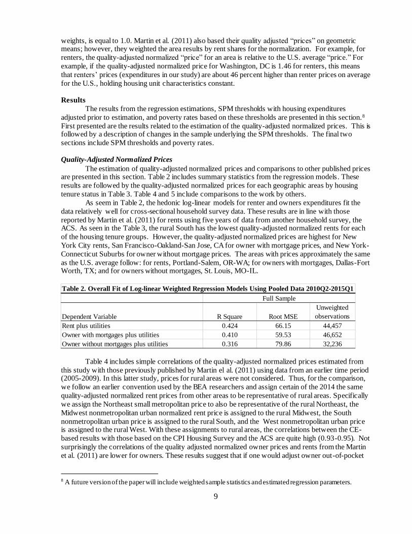
The estimation of quality-adjusted normalized prices and comparisons to other published prices are presented in this section. Table 2 includes summary statistics from the regression models. These

results are followed by the quality-adjusted normalized prices for each geographic areas by housing

tenure status in Table 3. Table 4 and 5 include comparisons to the work by others.

As seem in Table 2, the hedonic log-linear models for renter and owners expenditures fit the

data relatively well for cross-sectional household survey data. These results are in line with those

reported by Martin et al. (2011) for rents using five years of data from another household survey, the ACS. As seen in the Table 3, the rural South has the lowest quality-adjusted normalized rents for each

of the housing tenure groups. However, the quality-adjusted normalized prices are highest for New

York City rents, San Francisco-Oakland-San Jose, CA for owner with mortgage prices, and New York-

Connecticut Suburbs for owner without mortgage prices. The areas with prices approximately the same

as the U.S. average follow: for rents, Portland-Salem, OR-WA; for owners with mortgages, Dallas-Fort Worth, TX; and for owners without mortgages, St. Louis, MO-IL.

Table 4 includes simple correlations of the quality-adjusted normalized prices estimated from

this study with those previously published by Martin el al. (2011) using data from an earlier time period (2005-2009). In this latter study, prices for rural areas were not considered. Thus, for the comparison,

we follow an earlier convention used by the BEA researchers and assign certain of the 2014 the same

quality-adjusted normalized rent prices from other areas to be representative of rural areas. Specifically

we assign the Northeast small metropolitan price to also be representative of the rural Northeast, the

Midwest nonmetropolitan urban normalized rent price is assigned to the rural Midwest, the South

nonmetropolitan urban price is assigned to the rural South, and the West nonmetropolitan urban price is assigned to the rural West. With these assignments to rural areas, the correlations between the CE-

based results with those based on the CPI Housing Survey and the ACS are quite high (0.93-0.95). Not

surprisingly the correlations of the quality adjusted normalized owner prices and rents from the Martin

et al. (2011) are lower for owners. These results suggest that if one would adjust owner out-of-pocket

8 A future version of the paper will include weighted sample statistics and estimated regression parameters.

Table 2. Overall Fit of Log-linear Weighted Regression Models Using Pooled Data 2010Q2-2015Q1

Dependent Variable R Square Root MSE

Unweighted

observations

Rent plus utilities 0.424 66.15 44,457

Owner with mortgages plus utilities 0.410 59.53 46,652

Owner without mortgages plus utilities 0.316 79.86 32,236

Full Sample

10

Renter

Rents +

Utilities

Mortgage Principal

and Interest,

Homeowner

Insurance, Property

Taxes, M&R +

Utilities

Homeowner

Insurance,

Property Taxes,

M&R + Utilities

PSU Area PSU Description

A102 Philadelphia-Wilmington-Atlantic City, PA-NJ-DE-MD 1.238 1.233 1.443

A103 Boston-Brockton-Nashua, MA-NH-ME-CT 1.276 1.399 1.682

A104 Pittsburgh, PA 0.827 0.901 1.110

A109 New York City 1.791 1.707 1.871

A110 New York-Connecticut Suburbs 1.555 1.696 2.295

A111 New Jersey-Pennsylvania Suburbs 1.558 1.659 2.227

A207 Chicago-Gary-Kenosha, IL-IN-WI 1.233 1.230 1.377

A208 Detroit-Ann Arbor-Flint, MI 0.894 0.970 1.155

A209 St. Louis, MO-IL 0.864 0.889 1.002

A210 Cleveland-Akron, OH 0.882 0.936 1.106

A211 Minneapolis-St. Paul, MN-WI 1.084 1.081 1.111

A212 Milwaukee-Racine, WI 0.956 1.116 1.352

A213 Cincinnati-Hamilton, OH-KY-IN 0.860 0.874 0.986

A214 Kansas City, MO-KS 0.863 0.875 0.989

A312 Washington, DC-MD-VA-WV 1.461 1.211 1.234

A313 Baltimore, MD 1.186 1.105 1.144

A316 Dallas-Fort Worth, TX 0.998 1.001 1.152

A318 Houston-Galveston-Brazoria, TX 0.957 0.960 1.180

A319 Atlanta, GA 0.958 0.848 0.831

A320 Miami-Fort Lauderdale, FL 1.194 1.038 0.944

A321 Tampa-St. Petersburg-Clearwater, FL 0.943 0.910 0.911

A419 Los Angeles-Long Beach, CA 1.425 1.477 1.158

A420 Los Angeles Suburbs, CA 1.170 1.178 0.974

A422 San Francisco-Oakland-San Jose, CA 1.532 1.781 1.291

A423 Seattle-Tacoma-Bremerton, WA 1.153 1.288 1.395

A424 San Diego, CA 1.410 1.467 1.075

A425 Portland-Salem, OR-WA 0.999 1.178 1.268

A426 Honolulu, HI 1.475 1.436 1.127

A427 Anchorage, AK 1.367 1.396 1.572

A429 Phoenix-Mesa, AZ 0.911 0.923 0.947

A433 Denver-Boulder-Greeley, CO 1.038 1.002 0.817

D200 Midwest nonmetropolitan urban 0.642 0.819 0.973

D300 South nonmetropolitan urban 0.726 0.774 0.738

D400 West nonmetropolitan urban 0.829 0.992 0.967

X100 Northeast small metroplitan 0.933 0.975 1.213

X200 Midwest small metropolitan 0.795 0.871 0.976

X300 South small metropolitan 0.829 0.827 0.802

X499 West small metropolitan 0.811 0.874 0.786

R100 Northeast rural 0.971 0.732 1.035

R200 Midwest rural 0.646 0.781 0.863

R300 South rural 0.615 0.721 0.683

R499 West rural 0.858 1.144 0.932

Weighted Geometric Mean 100.000 100.000 100.000

Geometric Means (Normalized)

Owner

Table 3. Quality-Adjusted Normalized Renter and Owner Expenditures by Primary Sample Unit (PSU)Areas: CE

Interview Data 2010Q2-2015Q1

11

spending by quality-adjusted normalized rents, resulting thresholds would not adequately reflect the

prices faced by owners.

CE-based quality-adjusted normalized prices are compared to Median Rent Indexes (MRI) for

2014 in Table 5. As noted earlier, the MRIs are applied to the “national” thresholds in order to produce

subnational. MRIs are based on gross rents plus utilities as collected in the American Community Survey. Based on an examination of the maximum and minimum rents, the two sources of data result in

similar values. The quality adjusted normalized owner with mortgage values are close as well;

however, those for owners without mortgage diverge the most. In Chart 1 rent indexes for a select

number of geographic areas are shown. CE-based area indexes are presented in comparison to MRIs

from the ACS. Although we do not recommend that the ACS indexes to adjust micro-level housing expenditures before estimating the FCSU thresholds, seeing how well the CE indexes compare provides

us reassurance regarding the modeling approach that we use. Areas indexes are produced for the

following areas for both the CE and ACS: Washington, DC, Baltimore, MD, Los Angeles-Long Beach,

CA, and San Francisco-Oakland, CA. Only one index is available from the ACS for the New York City

and surrounding area. However, with the CE we are able to produce indexes for three areas within the New York City area, The CE disaggregation suggests that differences in prices within the area are

important.

Table 4. Correlations of CE Based Normalized Rent Prices with CPI and ACS Normalized Rent Prices

CPI Housing Survey (2005-2009) ACS (2005-2009)

Renter shelter and utilities 0.951 0.931

Owner with mortgages shelter and utilities 0.913 0.861

Owner without mortgages shelter and utilities 0.633 0.546

BEA Quality Adjusted Normalized Rent Prices

CE Quality-Adjusted Normalized Rent Prices

(2010Q2-2015Q1)

Table 5. Comparison of CE-Based Quality-Adjusted Normalized Prices and Median Rent Indexes: 2014

ACS

Renter S+UOwner with

Mortgage S+U

Owner without

Mortgage S+UMRI 2014

a

Maximum 1.791 1.781 2.290 1.782

Minimum 0.615 0.721 0.680 0.595

Range 1.176 1.060 1.610 1.187

Ratio of Max to Min 2.912 2.470 3.368 2.996a Based on 5-year American Community Survey median rents for 2-bedroom apartments with complete kitchens and full baths (Renwick 2017).

CE Interview Survey

12

SPM Sample and Thresholds

The impact of adjusting housing expenditures, by CE-based quality-adjusted normalized prices

before producing the SPM thresholds, on the underlying sample and thresholds are presented in this

section. Housing expenditures (not including those for telephone) for each consumer unit (CU) in the

CE Interview Survey are adjusted by one of the area specific quality-adjusted normalized prices based on the geographic area where the CU lives and the CU’s housing tenure. These adjusted housing

expenditures are added to price unadjusted expenditures for food, clothing, and telephone. Next these

FCSU expenditures are converted to 2014 dollars using the all items CPI-U U.S. City Average. FCSU

expenditures for the estimation sample of CUs with two children are further adjusted using the 3-

parameter equivalence scale; this results in equivalized FCSU expenditures for two adults with two children, the reference SPM unit. Changes in the underlying SPM reference samples and thresholds,

resulting from applying quality-adjusted normalized prices to individual CU housing expenditures, are

presented in this section.

Underlying Weighted Sample. As noted earlier, SPM thresholds are based on the 30-36th

percentile range of 2-adult-2-child equivalized FCSU expenditures. When the CE-based quality-adjusted normalized prices are applied to CU level housing expenditures initially, as proposed in this

study, the ranking of FCSU changes. The new ranking results in a larger percentage of owners without

mortgages (from 10.8% to 12.5% of the sample) and renters (47.6% to 48.4%) with a reduction in the

owners with mortgages (41.5% to 39.2%). Regional changes also result with the Northeast gaining

greater representation in the weighted sample (from 12.8% to 19.1%); the South losses the most by 3.8

percentage points (from 41.7 % to 37.9%); while the representation by the Midwest and West remains about constant around 22 percent. When examined with respect to the 42 geographic areas underlying

the CE-based normalized prices, we find the largest percentage gains for the New York-Connecticut

suburbs and the largest losses for the South small metropolitan area.9

SPM Thresholds for Two Adults with Two Children. SPM thresholds for the reference unit

are presented in Table 6. Three sets of thresholds are presented: (1) currently published (BLS 2017); (2) thresholds based on telephone not being included in utilities; and (3) thresholds with the CE-based

quality-adjustment to shelter and non-telephone utility expenditures. In all instances, the thresholds for

owners with mortgages are highest, followed by those for renters and then owners without mortgages.

Not including telephone services as part of utilities results in a decrease of $310 for owners without

mortgages; thresholds for the other two group also decrease by minimally. When housing expenditures (again not including telephone services) are adjusted for by CE-based quality-adjusted normalized

prices, SPM thresholds for owners with mortgages increase by $483 (or 1.9%), they increase by $612

(or 2.9%) for owners without mortgages, and by $264 (or 1.0%) for renters .

For the 2-adult-w-child SPM “national” thresholds to be adjusted to produce subnational thresholds, the housing shares of the thresholds are needed as it is only the housing portion of the

thresholds that are adjusted by the MRI (see equation 6).10 Housing expenditure shares implicit in the

2014 SPM thresholds are presented in Table 7. Not surprisingly, the shares for utilities fall due to the omission of telephone from utilities with the greatest percentage point decrease for owners without

9 A chart showing the distributions of weighted CUS by housing tenure based on the published, unpriced adjusted ranking, and based on the price adjusted housing expenditures is available upon request. 10 For a discussion of geographic adjustment methods and research, see Renwick (2011). Also see Ziliak (2010).

Table 6. 2-Adult-2Child SPM Thresholds without and with CE-Based Quality-Adjusted Normalized Price Adjustment: 2014

Housing Expenditures Adjusted

Published Utilities do not include Telephone Utilities do not include Telephone

Owners with mortgages $25,844 $25,840 $26,327

Owners without mortgages $21,380 $21,070 $21,992

Renters $25,460 $25,534 $25,724

Housing Expenditures Not Adjusted

13

mortgages (5.8 percentage points). The housing shares of the thresholds drops from 50.7% (published) to 45.1% (with price adjustment and telephone not in utilities) for owners with mortgages, for renters it

50% to 43.8% for renters, and 40.4% to 34.4% for owners without mortgages.

Chart XX includes population poverty rates based on the three threshold concepts after than

have been further adjusted to account for differing numbers of adults and children and after adjustments to produce subnational thresholds that reflect differences in the cost of housing. Resources are

compared to SPM threshold to produce poverty rates for the U.S. population using data from the

Current Population Survey Annual Social and Economic Supplement. Poverty rates are produced for

the year 2014.

Poverty Rates Poverty rates are presented in Table 8 with and without telephone services included in housing,

and with and without the CE-based normalized price adjustments applied to housing expenditures before estimating the 2-adult-2child SPM thresholds. AS noted earlier, before poverty rates could be

produced using these thresholds, they were adjusted to account for different numbers of adults and

children and also to reflect median rents for areas as defined in the ACS by Renwick. Overall poverty

increased with the CE-based housing price adjustments, from 15.3% to 15.8 % of the population. For

thresholds with the CE-price adjustment, including telephone as part of utilities impacted people living outside metropolitan statistical areas (with an increase from 13.3% to 13.9%). Few other differences

resulted.

Discussion and Conclusion

In the SPM thresholds used for poverty statistics, implicit differences in prices across areas

exist. The underlying assumption is that these differences do not matter. However, this assumption is largely untested, with the possible exception of Bishop et al (2017). The purpose of this study was to

examine the impact of accounting for spatial differences in housing prices across areas before

estimating the SPM thresholds, and thus to make adjustments at the consumer unit level. To do this,

first quality-adjusted normalized prices were produced using CE data, the same data that are used for

the production of the SPM thresholds. Normalized area-specific prices were produced separately for owners with mortgages, owners without mortgages, and renters. The CE data were used in order to

account for prices faced by renters and owners for shelter and utilities in their out-of-pocket

expenditures. The normalized prices produced in this study, at least for a select number of areas, are

quite similar to those produced by Renwick (2017) using gross rents from the American Community

Table 7. Housing Shares of 2-Adult-2-Child SPM Thresholds: 2014

Published

Utilities do not include

Telephone

Utilities include

Telephone

Utilities do not

include Telephone

Owners with Mortgages

shelter 34.1% 34.1% 34.1% 34.1%

utilities 16.6% 13.5% 16.6% 11.1%

housing total 50.7% 47.7% 50.6% 45.1%

Renters

shelter 36.4% 36.3% 35.5% 35.5%

utilities 13.6% 8.2% 13.9% 8.3%

housing total 50.0% 44.5% 49.5% 43.8%

Owners without mortgages

shelter 18.3% 18.5% 17.9% 17.9%

utilities 22.2% 14.2% 23.0% 16.4%

housing total 40.4% 32.7% 40.9% 34.3%

Housing Expenditures AdjustedHousing Expenditures Not Adjusted

14

Survey. Other indexes that account for differences by area are the rent regional price parities (RPPs), and food-apparel-rent FAR RPPs (Renwick et al. 2017). However, these are not based on the same

geography as the SPM thresholds nor are the definitions of housing expenditures the same.

A goal of this study was to develop a prototype approach is to adjust consumer unit specific

housing expenditures for consumer unit expenditures underlying the SPM thresholds. Although the

impact on SPM poverty rates appears to be small, we think that these underlying differences are importance and should be accounted for before estimation “national” thresholds. Future work includes

refining the hedonic model used to produce the normalized area-specific prices to account for

geographic areas. Another avenue of research to consider is a multilateral index methodology that

accounts for the full bundle of FCSU, more like the FAR PPPs produced by Renwick et al. (2017).

References

Aten, Bettina, Eric Figueroa, and Troy Martin, “Notes on Estimating the Multi-Year Regional Price Parities by 16 Expenditure Categories: 2005-2009,” 2011,

https://www.bea.gov/papers/pdf/notes_on_estimating_the_multi_year_rpps_and_appendix_tables.pdf .

Bishop, John, Jonathan Less, and Lester A. Zeager, “Improving the Supplemental Poverty Measure:

Two Proposals,” unpublished manuscript available from the authors, Department of Economics, East Carolina University, Greenville, NC, March 8, 2017.

Bureau of Labor Statistics (BLS), Division of Price and Index Number Research, PINR Experimental

Poverty Measures, http://stats.bls.gov/pir/spmhome.htm , 2017.

Census Bureau (Census), “American Community Survey and Puerto Rico Community Survey 2016

Subject Definitions, https://www2.census.gov/programs-

surveys/acs/tech_docs/subject_definitions/2016_ACSSubjectDefinitions.pdf .

Citro, Connie F. and Robert T. Michael (eds.), Measuring Poverty: A New Approach, National

Academy of Sciences, Washington, DC, 1995.

Table 8. Percentage of SPM Poor Based on Published SPM Thresholds with and without Housing Adjusted

Utilities include

Telephone

Utilities do not include

Telephone

15.3 15.8 15.8

Residence

Outside metropolitan

statistical areas 12.8 13.3 13.9

Outside principal cities 13.1 13.7 13.5

Inside principal cities 20.2 20.6 20.6

Inside metropolitan statistical

ares 15.8 16.3 16.2

Region

West 18.4 18.7 18.4

South 15.6 16.3 16.5

Midwest 11.8 12.2 12.5

Northeast 14.7 15.1 15.0

Tenure

Renter 26.1 26.6 26.7

Owner/no mortgage/rentfree 13.0 13.7 13.7

Owner/mortgage 8.1 8.4 8.4

Housing Expenditures Adjusted

Published

All People

15

Figueroa, Eric, Bureau of Economic Analysis, unpublished “results of 1st Stage rents RPPs for 2015 and

2015 for the 38 metropolitan and urban areas of the U.S. using the CPI housing sample,” email

communication, September 21, 2017.

Fox, Liana, “The Supplemental Poverty Measure: 2016,” Current Population Reports, P60-261, U.S. Census Bureau, available at https://www.census.gov/content/dam/Census/library/publications/2017/demo/p60-261.pdf , September 2017. Interagency Technical Working Group (ITWG), “Observations from the Interagency Technical

Working Group on Developing a Supplemental Poverty Measure,” available at

http://stats.bls.gov/pir/spmhome.htm, 2010.

Kingkade, W. Ward, “What are Housing Assistance Support Recipients Reporting as Rent?” SEHSD Working Paper 2017-44, 9/12/2017,

https://www.census.gov/content/dam/Census/library/working-papers/2017/demo/SEHSD-WP2017-

44.pdf .

Martin, Troy, Bettina Aten, and Eric Figueroa, “Estimating the Price of Rents in Regional Price Parities,” manuscript from the Bureau of Economic Analysis, Department of Commerce, 2011,

https://www.bea.gov/papers/pdf/Estimating_Price_Rents_Regional_Price_Parities.pdf

Penvose, Jessica, BLS, “regarding questions about rents in the CPI data base used by BEA--three more

questions,” email communication, October 26, 2017.

Renwick, Trudi J., “Geographic Adjustments of Supplemental Poverty Measure Thresholds: Using the

American Community Survey Five-Year Data on Housing Costs,” paper presented at the July 2011

Western Economic Association, San Diego, CA, available from Census Bureau working papers, 2011a.

Renwick, Trudi, “Geographic Adjustments for SPM Poverty Thresholds,” presented at the Annual Meeting of the Allied Social Science Associations (ASSA), Society of Government Economists Session

(SGE), Denver, Colorado. Poverty Measurement Working Paper, U.S. Census Bureau, 2011b.

Renwick, Trudi J., unpublished poverty rates for 2014 based on SPM thresholds produced in this study

along with CPS data and SPM resource measure, December 1, 2017.

Renwick, Trudi J., Eric B. Figueroa, and Bettina H. Aten, “Supplemental Poverty Measure: A

Comparison of Geographic Adjustments with Regional Price Parities vs. Median Rents from the

American Community Survey,” available from Census Bureau working papers, March 2014.

Renwick, Trudi J., Eric B. Figueroa, and Bettina H. Aten, “Supplemental Poverty Measure: A Comparison of Geographic Adjustments with Regional Price Parities vs. Median Rents from the

American Community Survey: An Update,” SEHSD Working Paper Number 2017-36,

https://www.census.gov/content/dam/Census/library/working-papers/2017/demo/SEHSD-WP2017-

36.pdf .

Short, Kathleen, “The Research Supplemental Poverty Measure: 2010,” Current Population Reports,

P60-241, U.S. Census Bureau, available at www.census.gov/content /dam/Census/library

/publications/2011/demo /p60-241.pdf , November 2011.

16

Short, Kathleen, “Where We Live: Geographic Differences in Poverty Thresholds,” United States Bureau of the Census, paper presented at the Annual Meeting of the Society of Government

Economists, New Orleans, LA, 2001.

17

Area Area Description

A102 Philadelphia-Wilmington-Atlantic City, PA-NJ-DE-MD

A103 Boston-Brockton-Nashua, MA-NH-ME-CT

A104 Pittsburgh, PA

A109 New York City

A110 New York-Connecticut Suburbs

A111 New Jersey-Pennsylvania Suburbs

A207 Chicago-Gary-Kenosha, IL-IN-WI

A208 Detroit-Ann Arbor-Flint, MI

A209 St. Louis-East St. Louis-Alton, MO-IL

A210 Cleveland-Akron, OH

A211 Minneapolis-St. Paul, MN-WI

A212 Milwaukee-Racine, WI

A213 Cincinnati-Hamilton, OH-KY-IN

A214 Kansas City, MO-KS

A312 Washington, DC-MD-VA-WV

A313 Baltimore, MD

A316 Dallas-Fort Worth, TX

A318 Houston-Galveston-Brazoria, TX

A319 Atlanta, GA

A320 Miami-Fort Lauderdale, FL

A321 Tampa-St. Petersburg-Clearwater, FL

A419 Los Angeles-Long Beach, CA

A420 Los Angeles Suburbs, CA

A422 San Francisco-Oakland-San Jose, CA

A423 Seattle-Tacoma-Bremerton, WA

A424 San Diego, CA

A425 Portland-Salem, OR-WA

A426 Honolulu, HI

A427 Anchorage, AK

A429 Phoenix-Mesa, AZ

A433 Denver-Boulder-Greeley, CO

D200 Midwest nonmetropolitan urban

D300 South nonmetropolitan urban

D400 West nonmetropolitan urban

X100 Northeast small metroplitan

X200 Midwest small metropolitan

X300 South small metropolitan

X499 West small metropolitan

R100 Northeast rural

R200 Midwest rural

R300 South rural

R400 West rural

In CE Sample Only

In CPI Housing Survey Sample and CE Sample

Table 1. Areas for Which Quality-Adjusted Normalized Prices Are Produced