Controlled Braking for Omnidirectional...
10
International Journal of Control Science and Engineering 2013, 3(2): 48-57 DOI: 10.5923/j.control.20130302.03 Controlled Braking for Omnidirectional Wheels Viktor Kálmán Department of Control Engineering and Information Technology, Budapest University of Technology and Economics, Budapest, 1117, Hungary Abstract Due to their design omnidirectional wheels in general lack the capability to generate substantial side forces - forces perpendicular to the roller axis. This is caused by the free rolling rollers around the circumference, the very same thing that allows holonomic movement. An interesting consequence is that when an omnidirectional platform undergoes heavy braking, due to uneven wheel load or other disturbances, the vehicle has a tendency to swerve. An omnidirectional platform is a complex nonlinear system, where the nonlinearities come from the wheel material and construction, and the unidirectional force generation capability. In this article a corrective controller is described that prevents swerving even in the presence of high uncertainties. The operation and disturbance rejection of the controller is demonstrated by simulation in Modelica-Dymola environment. Keywords Omnidirectional Wheel, Brake Assistant, Mobile Robot, Simulation, Modelica 1. Introduction Modern logistics systems pose high demands on mobile transportation, transport vehicles have to be agile, precise and safe. Omnidirectional wheels provide holonomic movement capabilities, allowing vehicles to change their direction of movement, without changing their orientation. This superior maneuverability makes them an attractive choice for logistic vehicles. The invention of these special wheels dates back to the seventies[1], and they have been used in countless applications both by hobbyists, industrial companies and researchers since then. They have been successfully used in forklifts and other transport machines like the Sidewinder from Airtrax, or the OmniMove platform family from KUKA Robotics and others[2]. They also attract a considerable amount of researchers, who strive to enhance their mechanical capabilities and control algorithms[3],[4], [5]. Figure 1 demonstrates some of the various applications in which they are being used today. Their advantages however come at a price: they require complex mechanical design, independent drivetrain for each wheel and smart control algorithms. 1.1. Motivation Omnidirectional wheels consist of several – usually rubber coated – rollers around the wheels circumference, the most popular angles are 45° and 0°, the first is usually called Mecanum, or Swedish wheel (Figure 2.), the latter is usually * Corresponding author: [email protected] (Viktor Kálmán) Published online at http://journal.sapub.org/control Copyright © 2013 Scientific & Academic Publishing. All Rights Reserved called Omni-wheel. The rollers are spinning freely, only the main axis is powered. Basically they can only exert force parallel to the rotational axis of the roller touching the ground. Because of this they have no self aligning moment, or side force generation capabilities, so they do not keep their rolling direction when pushed or braked, as opposed to a vehicle with conventional tires. Figure 1. Examples for the use of omnidirectional wheels 1 Since the load distribution and mass of a transport robot changes each time the cargo is changed, it is quite hard to predict actual load distribution, and in consequence, the resulting friction forces during a braking maneuver. Unbalanced forces generate a torque around the center of gravity, turning the platform, until equilibrium is reached 1www.airtrax.com, www.kuka-omnimove.com, [20], [21], [22]
Transcript of Controlled Braking for Omnidirectional...
International Journal of Control Science and Engineering 2013, 3(2): 48-57 DOI: 10.5923/j.control.20130302.03
Controlled Braking for Omnidirectional Wheels
Viktor Kálmán
Department of Control Engineering and Information Technology, Budapest University of Technology and Economics, Budapest, 1117, Hungary
Abstract Due to their design omnidirectional wheels in general lack the capability to generate substantial side forces - forces perpendicular to the roller axis. This is caused by the free rolling rollers around the circumference, the very same thing that allows holonomic movement. An interesting consequence is that when an omnidirectional p latform undergoes heavy braking, due to uneven wheel load or other disturbances, the vehicle has a tendency to swerve. An omnid irectional p latform is a complex nonlinear system, where the nonlinearit ies come from the wheel material and construction, and the unidirectional force generation capability. In this article a correct ive controller is described that prevents swerving even in the presence of high uncertainties. The operation and disturbance rejection of the controller is demonstrated by simulation in Modelica-Dymola environment.
Keywords Omnidirect ional Wheel, Brake Assistant, Mobile Robot, Simulat ion, Modelica
1. Introduction Modern logistics systems pose high demands on mobile
transportation, transport vehicles have to be agile, precise and safe. Omnidirectional wheels provide holonomic movement capabilities, allowing vehicles to change their direction of movement, without changing their orientation. This superior maneuverability makes them an attractive choice for logistic vehicles.
The invention of these special wheels dates back to the seventies[1], and they have been used in countless applications both by hobbyists, industrial companies and researchers since then. They have been successfully used in forklifts and other transport machines like the Sidewinder from Airtrax, or the OmniMove platform family from KUKA Robotics and others[2]. They also attract a considerable amount of researchers, who strive to enhance their mechanical capabilit ies and control algorithms[3],[4], [5]. Figure 1 demonstrates some of the various applications in which they are being used today.
Their advantages however come at a price: they require complex mechanical design, independent drivetrain for each wheel and smart control algorithms.
1.1. Motivation
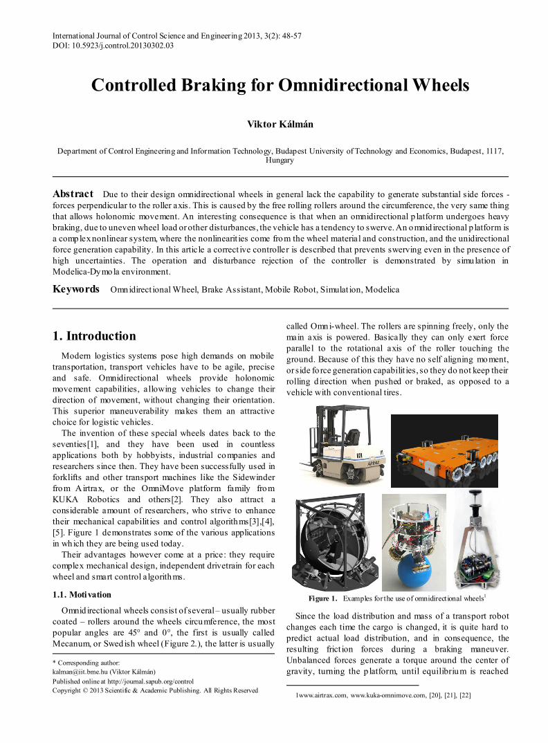
Omnid irectional wheels consist of several – usually rubber coated – rollers around the wheels circumference, the most popular angles are 45° and 0°, the first is usually called Mecanum, or Swedish wheel (Figure 2.), the latter is usually
* Corresponding author: [email protected] (Viktor Kálmán) Published online at http://journal.sapub.org/control Copyright © 2013 Scientific & Academic Publishing. All Rights Reserved
called Omni-wheel. The rollers are spinning freely, only the main axis is powered. Basically they can only exert force parallel to the rotational axis of the roller touching the ground. Because of this they have no self aligning moment, or side fo rce generation capabilit ies, so they do not keep their rolling d irection when pushed or braked, as opposed to a vehicle with conventional tires.
Figure 1. Examples for the use of omnidirectional wheels1
Since the load distribution and mass of a transport robot changes each time the cargo is changed, it is quite hard to predict actual load distribution, and in consequence, the resulting frict ion forces during a braking maneuver. Unbalanced forces generate a torque around the center of gravity, turning the p latform, until equilibrium is reached
1www.airtrax.com, www.kuka-omnimove.com, [20], [21], [22]
International Journal of Control Science and Engineering 2013, 3(2): 48-57 49
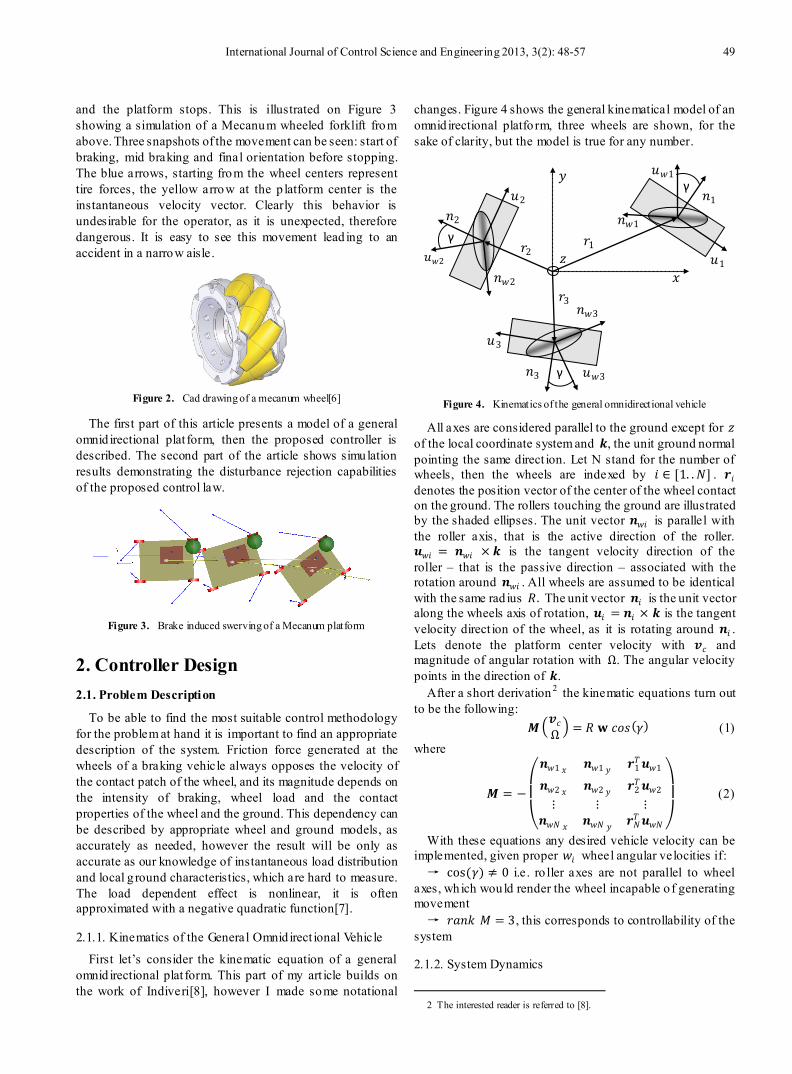
and the platform stops. This is illustrated on Figure 3 showing a simulation of a Mecanum wheeled forklift from above. Three snapshots of the movement can be seen: start of braking, mid braking and final orientation before stopping. The blue arrows, starting from the wheel centers represent tire forces, the yellow arrow at the p latform center is the instantaneous velocity vector. Clearly this behavior is undesirable for the operator, as it is unexpected, therefore dangerous. It is easy to see this movement lead ing to an accident in a narrow aisle.
Figure 2. Cad drawing of a mecanum wheel[6]
The first part of this article presents a model of a general omnid irectional plat form, then the proposed controller is described. The second part of the article shows simulation results demonstrating the disturbance rejection capabilities of the proposed control law.
Figure 3. Brake induced swerving of a Mecanum platform
2. Controller Design 2.1. Problem Description
To be able to find the most suitable control methodology for the problem at hand it is important to find an appropriate description of the system. Friction force generated at the wheels of a braking vehicle always opposes the velocity of the contact patch of the wheel, and its magnitude depends on the intensity of braking, wheel load and the contact properties of the wheel and the ground. This dependency can be described by appropriate wheel and ground models, as accurately as needed, however the result will be only as accurate as our knowledge of instantaneous load distribution and local g round characteristics, which are hard to measure. The load dependent effect is nonlinear, it is often approximated with a negative quadratic function[7].
2.1.1. Kinematics of the General Omnid irect ional Vehicle
First let’s consider the kinematic equation of a general omnid irectional plat form. This part of my art icle builds on the work of Indiveri[8], however I made some notational
changes. Figure 4 shows the general kinematical model of an omnid irectional platfo rm, three wheels are shown, for the sake of clarity, but the model is true for any number.
Figure 4. Kinematics of the general omnidirectional vehicle
All axes are considered parallel to the ground except for 𝑧𝑧 of the local coordinate system and 𝒌𝒌, the unit ground normal pointing the same direct ion. Let N stand for the number of wheels, then the wheels are indexed by 𝑖𝑖 ∈ [1. .𝑁𝑁] . 𝒓𝒓𝑖𝑖 denotes the position vector of the center of the wheel contact on the ground. The rollers touching the ground are illustrated by the shaded ellipses. The unit vector 𝒏𝒏𝑤𝑤𝑖𝑖 is parallel with the roller axis, that is the active direction of the roller. 𝒖𝒖𝑤𝑤𝑖𝑖 = 𝒏𝒏𝑤𝑤𝑖𝑖 × 𝒌𝒌 is the tangent velocity direction of the roller – that is the passive direction – associated with the rotation around 𝒏𝒏𝑤𝑤𝑖𝑖 . All wheels are assumed to be identical with the same rad ius 𝑅𝑅. The unit vector 𝒏𝒏𝑖𝑖 is the unit vector along the wheels axis of rotation, 𝒖𝒖𝑖𝑖 = 𝒏𝒏𝑖𝑖 × 𝒌𝒌 is the tangent velocity direct ion of the wheel, as it is rotating around 𝒏𝒏𝑖𝑖 . Lets denote the platform center velocity with 𝒗𝒗𝑐𝑐 and magnitude of angular rotation with Ω. The angular velocity points in the direction of 𝒌𝒌.
After a short derivation 2 the kinematic equations turn out to be the following:
𝑴𝑴�𝒗𝒗𝑐𝑐Ω � = 𝑅𝑅 𝐰𝐰 𝑐𝑐𝑐𝑐𝑐𝑐(𝛾𝛾) (1) where
𝑴𝑴 = −
⎝
⎜⎛𝒏𝒏𝑤𝑤1 𝑥𝑥 𝒏𝒏𝑤𝑤1 𝑦𝑦 𝒓𝒓1
𝑇𝑇𝒖𝒖𝑤𝑤1
𝒏𝒏𝑤𝑤2 𝑥𝑥 𝒏𝒏𝑤𝑤2 𝑦𝑦 𝒓𝒓2𝑇𝑇𝒖𝒖𝑤𝑤2
⋮ ⋮ ⋮𝒏𝒏𝑤𝑤𝑁𝑁 𝑥𝑥 𝒏𝒏𝑤𝑤𝑁𝑁 𝑦𝑦 𝒓𝒓𝑁𝑁𝑇𝑇 𝒖𝒖𝑤𝑤𝑁𝑁 ⎠
⎟⎞
(2)
With these equations any desired vehicle velocity can be implemented, given proper 𝑤𝑤𝑖𝑖 wheel angular velocities if: → cos(𝛾𝛾) ≠ 0 i.e . ro ller axes are not parallel to wheel
axes, which would render the wheel incapable o f generating movement → 𝑟𝑟𝑟𝑟𝑟𝑟𝑟𝑟 𝑀𝑀 = 3, this corresponds to controllability of the
system
2.1.2. System Dynamics
2 The interested reader is referred to [8].
γ 𝑟𝑟1
𝑢𝑢1
𝑟𝑟𝑤𝑤1
𝑢𝑢𝑤𝑤1
γ
𝑟𝑟2 𝑢𝑢2
𝑟𝑟𝑤𝑤2 𝑢𝑢𝑤𝑤2
𝑟𝑟𝑤𝑤3
𝑢𝑢𝑤𝑤3 γ 𝑟𝑟3
𝑢𝑢3
𝑟𝑟2 𝑟𝑟1
𝑟𝑟3
𝑦𝑦
𝑥𝑥 𝑧𝑧
50 Viktor Kálmán: Controlled Braking for Omnidirectional Wheels
Forces and velocities of an omnidirectional p latform during braking are demonstrated through an example of a Mecanum plat form braking with nonzero angular velocity – Figure 5. It is assumed that the vehicle moves on a flat surface, consequently it has three degrees of freedom.
Figure 5. Forces and velocities during braking – illustration on a Mecanum platform
The system to be controlled is a MIMO system. Its state equation can be written in the general form:
�̇�𝒙 = 𝑓𝑓(𝒙𝒙,𝒖𝒖) (3) where the usual notations are used – 𝒙𝒙 is the state vector, 𝒖𝒖 is the input and 𝑓𝑓( ) is a nonlinear function. In the case of an accelerating mechanical system, the state vector consists of resulting linear and angular velocity of a reference point. However for this particu lar case – a braking omnid irect ional platform – it is more practical to also include 𝒗𝒗𝑖𝑖 wheel center velocities: 𝒙𝒙 = { 𝒗𝒗𝑖𝑖 ,𝒗𝒗𝑐𝑐 ,𝝎𝝎}′. These can be derived in a simple way from platform center linear and angular velocity.
𝒗𝒗𝑖𝑖 = 𝒗𝒗𝑐𝑐 + 𝝎𝝎 × 𝒓𝒓𝑐𝑐𝑖𝑖 (4) where 𝒓𝒓𝑐𝑐𝑖𝑖 is the vector pointing from the p latform center to a given wheel center.
The input vector consists of 𝑢𝑢(𝒇𝒇𝑖𝑖 (𝒇𝒇𝑑𝑑 )) a function of the friction force of the wheels and 𝒇𝒇𝒅𝒅 driver input. For the time being let’s assume a constant driver input 𝑢𝑢 = 𝒇𝒇𝑖𝑖 . System parameters do not change frequently, only when the payload is changed, therefore we can consider the system autonomous, or time invariant. The main dynamical equations can be derived from Newton’s law:
𝑚𝑚�̇�𝒗𝑐𝑐 = ∑ 𝒇𝒇𝑖𝑖i (5) 𝑱𝑱𝑐𝑐 �̇�𝛚 = ∑ 𝒇𝒇𝒊𝒊 × 𝒓𝒓𝑖𝑖𝑖𝑖 (6)
These equations are written for the geometrical center of the vehicle. Even these simplified equations contain various uncertain parameters, such as 𝑚𝑚 mass and 𝑱𝑱𝑐𝑐 inert ia tensor of the vehicle. Both can change with the load. Further uncertainty is added by the unknown magnitude of 𝒇𝒇𝑖𝑖 friction forces. They are generated to oppose wheel velocity and point in the active direction of the wheel i.e.:
𝒇𝒇𝑖𝑖 = 𝜉𝜉𝑖𝑖 𝒏𝒏𝑤𝑤𝑖𝑖 (𝒏𝒏𝑤𝑤𝑖𝑖 ‖−𝒗𝒗i‖) (7) where 𝜉𝜉𝑖𝑖 is a nonlinear function describing dependence of the frict ion force on wheel load and ground characteristics, for a g iven driver input i.e . pressure on the brake pedal. 𝒏𝒏𝑤𝑤𝑖𝑖 is a unit vector pointing in the direction of the roller axis, ‖−𝒗𝒗𝑖𝑖‖ is a unit vector pointing in the opposing direction of the velocity of the given wheel center. See Figure 4 for notations.
Another important property of the system, that it is strongly cross coupled, all inputs have an effect on all state variables. This fo llows from equation (2).
2.1.3. Feedback
Measuring the state variables 𝒗𝒗𝑐𝑐 and 𝝎𝝎 is not a straightforward task for omnid irectional vehicles, because wheel rotation based methods, frequently used for vehicles with d ifferential, o r Ackermann drive would introduce large errors. I assume them to be measurable, for example by a method described in[9], which is especially suited for omnid irectional platfo rms. Th is method works much like an optical mouse, however with greater speed range and accuracy than similar works from the literature[10],[11]. 𝒗𝒗𝑖𝑖 can be calculated using equation (4).
2.1.4. Control Goals
In the previous sections I discussed the behavior of the plant and my conclusion is that even according to a simplified model, nonlinearit ies and parameter uncertainties due to unknown loads and changing ground characteristics make it impossible to prescribe an exact trajectory during braking. Instead of giving an exact trajectory the task can be handled by finding a compromise and describe the goal qualitatively. In the case of a braking omnid irect ional vehicle the control goal is twofold:
Goal 1: it is important to avoid directional change in the platforms movement
Goal 2: obviously it is also important to try and stop the platform as soon as possible
The goals are simple but several problems pose difficu lties in reaching them:
→ Since the wheels cannot be turned, the direction of force they generate only depends on the velocity direction of the contact patch, therefore the only option to assert control is to modulate the braking force.
→ Force generation is passive in a sense that it can only act to decrease velocity, and not to increase it.
→ Generally the friction forces of the wheels are not parallel with wheel velocities, therefore they will act to divert the platform from its original path, making the two goals contradictory.
→ From equations (1), (2) it is clear that any wheel effects both components of 𝒗𝒗𝑐𝑐 and 𝝎𝝎, consequently it is generally not possible to change a single degree of freedom of the platform independently.
The control loop is shown on Figure 6.
Figure 6. The control loop
2.1.5. Applicable Control Discipline
Because of the uncertainties and nonlinearities present in the system I decided to apply a nonlinear control approach.
controller
driver vehicle
𝒗𝒗𝑐𝑐 ,𝛚𝛚
𝑐𝑐
𝒗𝒗1
𝒗𝒗2
𝒗𝒗4
𝒇𝒇1
𝒇𝒇2
𝒇𝒇3 𝒇𝒇4
𝒗𝒗𝑐𝑐
𝑥𝑥0
𝑦𝑦0 𝑦𝑦 𝑥𝑥
𝒗𝒗3
𝜔𝜔
International Journal of Control Science and Engineering 2013, 3(2): 48-57 51
When controlling real dynamical systems uncertainties and disturbances in both the system model and the variables are a common problem. Effects of these uncertainties have to be taken into account in the controller design as they can severely impair control performance or even cause instability. Control of dynamical systems in the presence of heavy uncertainties has become an important subject of research. Due to the efforts made in this field many different approaches made considerable progress, such as nonlinear adaptive control, model pred ictive control and others.[12], [13],[14] These techniques are guaranteed to reach the control objectives in spite of modeling errors and parameter uncertainties.[15]
Imprecision may come from actual uncertainty about the plant, for example because of unknown parameters, or they might come into the model on purpose by using a simplified representation of the system’s dynamics. These uncertainties are classified as
→ structured - or parametric → unstructured - or unmodeled dynamics The first kind is actually included in the terms of the
model, the second corresponds to underestimation, or oversimplification of the system order.
Sliding mode control belongs in the family of robust control, because it is extremely tolerant of parameter inaccuracies. It is characterized by high simplicity. It utilizes discontinuous control laws to drive the system state trajectory onto a specified surface in the state space, the so called sliding or switching surface, and to keep the system state on this manifold after reaching it. Ev idently this approach only works when the control input is designed with sufficient authority to overcome the uncertainties and disturbances acting on the system. The main advantages are, that while the system is on the manifold it behaves like a reduced order system and system dynamics are insensitive to uncertainties and disturbances[16].
All these great advantages however come at a price, good performance can only be achieved with ext remely high control activity. This results in the so called chattering effect, which is the result of excitation of high frequency components of the system. Ideally control activity has an infinite switching frequency, which in real life applications is a high but finite frequency. High control activity also causes wear and tear of mechanical components. For further reading the reader is referred to:[17],[16],[15],[18] and others.
Formally the problem can be described as follows[15]: Let’s consider the following nonlinear system
𝑥𝑥̇(𝑡𝑡) = 𝑓𝑓(𝑡𝑡 , 𝑥𝑥) + 𝑔𝑔(𝑡𝑡 , 𝑥𝑥)𝑢𝑢(𝑡𝑡) (8) where 𝑥𝑥(𝑡𝑡) ∈ ℝ𝑟𝑟 , 𝑢𝑢(𝑡𝑡) ∈ ℝ𝑚𝑚 , 𝑓𝑓(𝑡𝑡 , 𝑥𝑥) ∈ ℝ𝑟𝑟×𝑟𝑟 and g(𝑡𝑡 , 𝑥𝑥) ∈ ℝ𝑟𝑟×𝑚𝑚 . The discontinuous feedback is given by:
𝑢𝑢𝑖𝑖 = �𝑢𝑢𝑖𝑖+ (𝑡𝑡 , 𝑥𝑥), 𝑖𝑖𝑓𝑓 𝜎𝜎𝑖𝑖(𝑥𝑥) > 0𝑢𝑢𝑖𝑖−(𝑡𝑡 , 𝑥𝑥), 𝑖𝑖𝑓𝑓 𝜎𝜎𝑖𝑖(𝑥𝑥) < 0
𝑖𝑖 = 1,2, … ,𝑚𝑚� (9)
where 𝜎𝜎𝑖𝑖(𝑥𝑥) = 0 is the 𝑖𝑖-th sliding surface, and 𝜎𝜎(𝑥𝑥) = [𝜎𝜎1(𝑥𝑥), 𝜎𝜎2(𝑥𝑥), …𝜎𝜎𝑚𝑚 (𝑥𝑥)]𝑇𝑇 = 0 (10)
is the (𝑟𝑟 − 𝑚𝑚) dimensional slid ing manifold. The control problem consist of developing the 𝑢𝑢𝑖𝑖+ , 𝑢𝑢𝑖𝑖−
functions and the sliding surface 𝜎𝜎(𝑥𝑥) = 0 , so that the closed-loop system exh ibits slid ing mode.
A sliding mode exists if, in the vicinity of the sliding surface the velocity vectors of the state trajectory are always directed towards the surface. In consequence if the state trajectory intersects the sliding surface, the value of the state trajectory remains within a neighborhood of the surface.
2.2. Omnidirectional Brake Assist
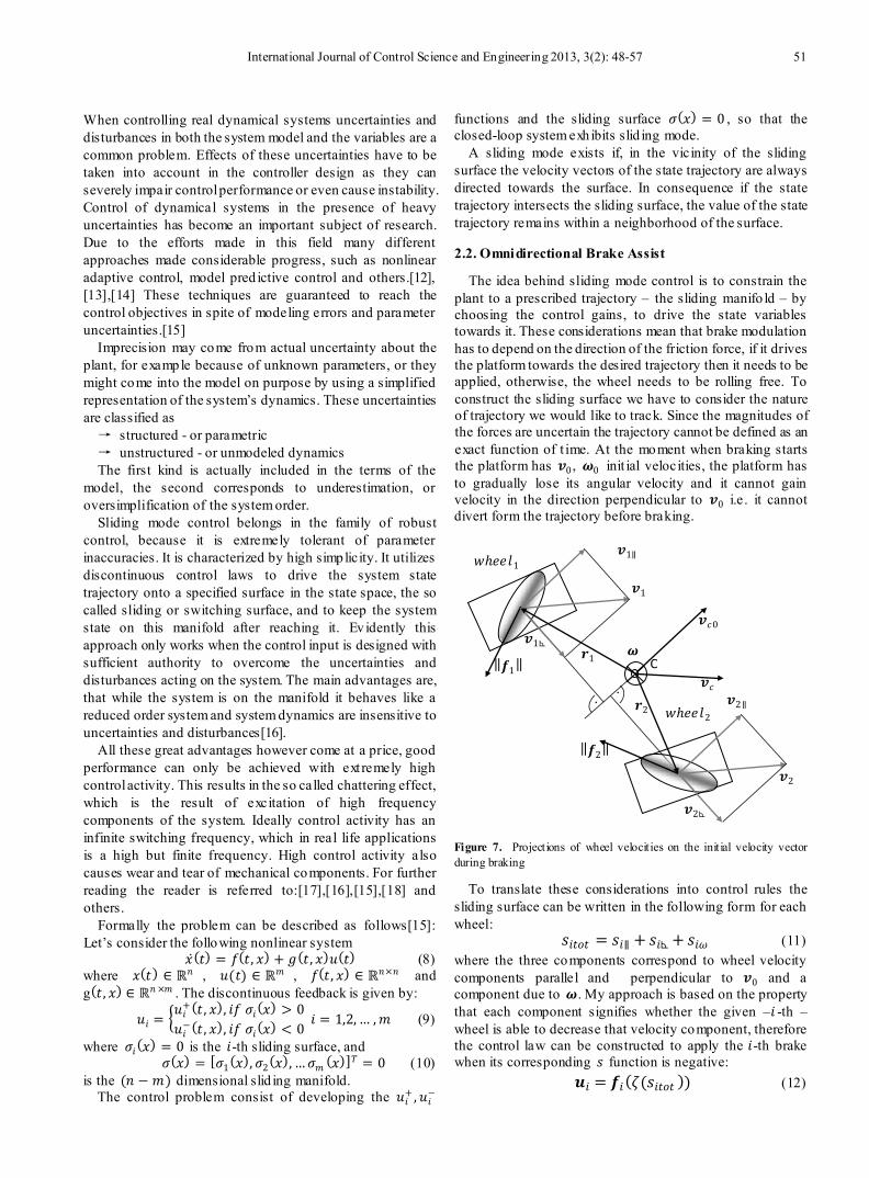
The idea behind sliding mode control is to constrain the plant to a prescribed trajectory – the sliding manifo ld – by choosing the control gains, to drive the state variables towards it. These considerations mean that brake modulation has to depend on the direction of the friction force, if it drives the platform towards the desired trajectory then it needs to be applied, otherwise, the wheel needs to be rolling free. To construct the sliding surface we have to consider the nature of trajectory we would like to track. Since the magnitudes of the forces are uncertain the trajectory cannot be defined as an exact function of t ime. At the moment when braking starts the platform has 𝒗𝒗0 , 𝝎𝝎0 init ial velocities, the platform has to gradually lose its angular velocity and it cannot gain velocity in the direction perpendicular to 𝒗𝒗0 i.e . it cannot divert form the trajectory before braking.
Figure 7. Projections of wheel velocities on the initial velocity vector during braking
To translate these considerations into control rules the sliding surface can be written in the following form for each wheel:
𝑐𝑐𝑖𝑖𝑡𝑡𝑐𝑐𝑡𝑡 = 𝑐𝑐𝑖𝑖∥ + 𝑐𝑐𝑖𝑖⊾ + 𝑐𝑐𝑖𝑖𝜔𝜔 (11) where the three components correspond to wheel velocity components parallel and perpendicular to 𝒗𝒗0 and a component due to 𝝎𝝎. My approach is based on the property that each component signifies whether the given –𝑖𝑖 -th – wheel is able to decrease that velocity component, therefore the control law can be constructed to apply the 𝑖𝑖-th brake when its corresponding 𝑐𝑐 function is negative:
𝒖𝒖𝑖𝑖 = 𝒇𝒇𝑖𝑖(𝜁𝜁(𝑐𝑐𝑖𝑖𝑡𝑡𝑐𝑐𝑡𝑡 )) (12)
. .
𝒗𝒗𝑐𝑐0
C
𝑤𝑤ℎ𝑒𝑒𝑒𝑒𝑙𝑙1
𝒗𝒗1
𝒗𝒗2
‖𝒇𝒇1‖
‖𝒇𝒇2‖
𝒗𝒗1⊾
𝒗𝒗2∥
𝒗𝒗2⊾
𝑤𝑤ℎ𝑒𝑒𝑒𝑒𝑙𝑙2
𝝎𝝎 𝒓𝒓1
𝒓𝒓2
𝒗𝒗𝑐𝑐
𝒗𝒗1∥
52 Viktor Kálmán: Controlled Braking for Omnidirectional Wheels
where
𝜁𝜁(𝑥𝑥) = � 0 𝑓𝑓𝑐𝑐𝑟𝑟 ∀ 𝑥𝑥 ≥ 01 𝑓𝑓𝑐𝑐𝑟𝑟 ∀ 𝑥𝑥 < 0
� 𝑥𝑥 ∈ ℝ (13)
Components of 𝑐𝑐𝑖𝑖𝑡𝑡𝑐𝑐𝑡𝑡 can be calcu lated the fo llowing way: 𝑐𝑐𝑖𝑖⊾ = ‖𝒇𝒇𝑖𝑖‖ 𝒗𝒗𝑖𝑖⊾ (14)
where 𝒗𝒗𝑖𝑖⊾ is the projection of 𝒗𝒗𝑖𝑖 on 𝒏𝒏𝑤𝑤𝑖𝑖 the direction of the roller axis of the wheel. Similarly
𝑐𝑐𝑖𝑖𝜔𝜔 = ‖𝜷𝜷𝑤𝑤𝑖𝑖 ‖𝛚𝛚|𝒓𝒓𝑐𝑐𝑖𝑖 | (15) where |𝒓𝒓𝑐𝑐𝑖𝑖 | is the distance from the p latform center to the wheel center, and
‖𝜷𝜷𝑤𝑤𝑖𝑖 ‖ = ‖𝒇𝒇𝑖𝑖 ‖ × ‖𝒓𝒓𝑐𝑐𝑖𝑖 ‖ (16) is the direct ion of the torque, or angular acceleration generated by 𝒇𝒇𝑖𝑖 . 𝒓𝒓𝑐𝑐𝑖𝑖 and the direction of ‖𝒇𝒇𝑖𝑖 ‖ are known from the geometry of the platform and they are generated to oppose the corresponding instantaneous wheel center velocities. 𝑐𝑐𝑖𝑖∥ is a different matter, the previously discussed two components change from wheel to wheel, the parallel component however can be decreased by any wheel in most cases, so if we calculate it from vector projections as in the case of 𝑐𝑐𝑖𝑖⊾ we interfere with Goal1. Let us insert a weighing function in the equation as follows:
𝑐𝑐𝑖𝑖∥ = 𝜓𝜓(‖𝒇𝒇𝑖𝑖‖ ,𝒗𝒗𝑖𝑖∥)‖𝒇𝒇𝑖𝑖‖𝒗𝒗𝑖𝑖∥ (17) where 𝒗𝒗𝑖𝑖∥ is the projection of 𝒗𝒗𝑖𝑖 on 𝒖𝒖𝑤𝑤𝑖𝑖 the direction perpendicular to the roller axis of the wheel, 𝜓𝜓( ) is a weighing function. The best way to define it is to make it angle dependent, large when the given roller is parallel with the velocity vector of its center – most efficient braking direction – and small otherwise. A suitable function I used is:
𝜓𝜓 = �−2 �2δi𝜋𝜋� + 2 − cos(δi )�
𝑟𝑟 (18)
where 𝛿𝛿𝑖𝑖 is the angle between the roller axis of the 𝑖𝑖 -th wheel and the parallel component of the wheel center velocity, 𝑟𝑟 is an odd integer, that scales the steepness of the function.
Note that all coefficients in the control equation are defined by platform geometry, that is considered to be constant and known in advance. 𝒗𝒗𝑖𝑖 , 𝝎𝝎 vectors are measured by feedback sensors.
2.2.1. Controller Characteristics
For every control system it is important to show that the closed loop system is stable and that it converges to the prescribed trajectory.
Let’s summarize the control strategy developed in section 2.2. A state dependent error function 𝒔𝒔𝑡𝑡𝑐𝑐𝑡𝑡 = 𝑓𝑓(𝒙𝒙) = 𝒔𝒔⊾ +𝒔𝒔ω + 𝒔𝒔∥ is defined for the platform, with three components corresponding to three degrees of freedom. The indiv idual brakes on the wheels are switched on and off according to the sign of this error function, as described by equations (12) and (13).
To find out if the closed loop control system is stable I decided to use the so called passivity approach[16] (p. 436). The passivity approach means that if the components in the feedback connection are passive in the sense that they do not generate energy on their own, then it is intuitively clear that the system will be passive. Generally a system is called
passive it there exists a storage function 𝑉𝑉(𝑡𝑡) ≥ 0, such that for all 𝑡𝑡0 < 𝑡𝑡1,
𝑉𝑉(𝑡𝑡1) ≤ 𝑉𝑉(𝑡𝑡0) + ∫ 𝑦𝑦(𝑡𝑡)𝑢𝑢(𝑡𝑡)𝑑𝑑𝑡𝑡𝑡𝑡1𝑡𝑡0
(19) where 𝑦𝑦 is the system output and 𝑢𝑢 is the input respectively. This equation simply states, that the energy (𝑉𝑉(𝑡𝑡)) of the system consists of the initial energy plus the supply rate 𝑦𝑦𝑢𝑢. If the equality holds, the system is lossless, if it is a strict inequality then the system is dissipative. For example energy is lost because of frict ion in mechanical systems, because of heat exchange in thermodynamical, or because of heat generation in electrical systems.
If we set the feedback to 𝑢𝑢 = −𝐾𝐾𝑦𝑦, where 𝐾𝐾 is a positive gain then it is guaranteed that the system energy remains bounded, thus the feedback system is stable. Considering an omnid irectional p latform in the context of my brake assist system, energy is stored in the form of kinetic energy. This can be written in the following form:
𝑉𝑉 = 𝑚𝑚𝑣𝑣𝑐𝑐2
2+ 𝐽𝐽ω2
2 (20)
considering the linear and rotational kinetic energ ies. The “supply rate” – in this case would be more appropriately called the “dissipation rate” – is the product of friction force and velocity which is essentially the power dissipated by braking the wheels. The goal of the braking maneuver is to drive the kinetic energy to zero. Brake forces are always generated to oppose movement causing negative acceleration. Since no energy is put in the system by the brake forces, it is evident that the system is passive and the inequality (19) holds true for ∀ 𝑡𝑡0, 𝑡𝑡1 time instants. However for a braking maneuver a strict inequality is needed for the vehicle to stop in a reasonable distance, which means that if we neglect small frict ional effects such as rolling resistance and bearing friction etc. a strict inequality can only be achieved if it is guaranteed that:
→ at least one brake is actuated at any time instant → with its active direction at an angle other than 90° to
the direction of movement The second criterion is guaranteed by design, if the vehicle
is created so that the rank of 𝑀𝑀 in equation (2) is 3, so that the vehicle is in fact useful. The first criterion means that the error function of at least one wheel has to be negative at all times. This is easily guaranteed if we add a rule for the controller that turns every brake on if ∀ 𝑐𝑐𝑖𝑖 ≥ 0.
3. Simulated Results
To demonstrate the capabilit ies of the brake assistant, I created a configurable omnidirect ional wheel model[19]. The model is based on the well known Rill t ire model[7], however its force generating capabilities have been changed to reflect the characteristics of a g iven omni-wheel. Figure 8 shows a simple sketch of the idea behind the transformation, slip is calculated in the “active” direction i.e. the direction of the axle of the ro ller on the ground, then driving forces are calculated according to this modified slip. Forces in the free-rolling – “passive” – direct ion are neglected fo r sake of simplicity. The advantage of the underlying Rill model is
International Journal of Control Science and Engineering 2013, 3(2): 48-57 53
that wheel parameters have physical meaning, they correspond to material stiffness, damping etc. thus they can be set reasonably well by educated guess, as opposed to other tire models where the parameters have to be set by measurements.
Figure 8. A regular t ire model with modified slip and force characteristics
I created two simple platfo rms using Modelica3 language in the Dymola simulation environment. These are the most preferred omnidirectional configurations, their rendered images are shown on Figure 9.
Figure 9. The most popular omnidirectional platforms in simulation, rendered by Dymola (rollers are not rendered for sake of effectiveness)
Note that the details of wheel geometry are not shown in the animat ion. The first platform is a simplified industrial forklift, it has four wheels, with ro llers mounted at a 45° angle (Mecanum wheels). I used lumped dynamic models. The vehicle body is represented by a point mass with inertia, and the load is represented by a simple point mass. Both the position and value of the masses, as well as vehicle dimensions are configurable. I also built a model of a three wheeled robot, with 0° rollers. Its body is represented by a point mass with inertia.
Speed measurement feedback can be realized by any convenient method, however I propose an optical speed sensor mounted on the platform, described in[9]. The sensor measures true ground speed, and angular velocity, and works much like a conventional optical mouse. In the simulation the sensor is included by quantizing the simulated platform linear and angular speed values with a zero order hold, and adding random noise.
3 https://modelica.org
Braking is realized by simulated hydraulic disc brakes mounted on the driveshaft; a wheel can be either driven by a torque (motor), slowed or stalled by braking or let to ro ll freely.
The control loop works the following way: When the “driver” – o r “autopilot” – pushes the brake pedal i.e. commanded brake fo rce surpasses a limit, the brake assist gets activated and the value of 𝒗𝒗𝑐𝑐0 , current linear velocity is stored. While braking, instantaneous wheel center velocities are calculated according to equation (4), based on the instantaneous platform velocity values 𝒗𝒗𝑐𝑐 and 𝛚𝛚, that are “measured” by an optical feedback unit. During the braking maneuver the controller continuously evaluates the 𝑐𝑐𝑖𝑖𝑡𝑡𝑐𝑐𝑡𝑡 error functions for each wheel. Based on the sign of the 𝑖𝑖-th error function the actuator at the 𝑖𝑖-th wheel lets the brake activate, – the brake fo rce asserted by the “driver” gets applied – or inhibits braking – lets the wheel ro ll freely. For practical reasons, to avoid low speed drift, the brake assist is only active above a certain velocity threshold, below that it is switched off, and all the brakes are activated normally.
3.1. Idealized Experiment
Figure 10. Braking in a straight line – snapshots, slowing from 10m/s
Figure 10 shows a demonstration of the brake assistant, with no external disturbances. The figure shows snapshots from an animation of an emergency braking trajectory at regular intervals. The upper part shows a run with the brake assist deactivated, the lower part shows the same experiment with the brake assist activated. Initial velocity is 10m/s. The difference between the two trajectories is obvious, with the brake assist activated, the vehicle does not swerve, but keeps its initial d irection of movement.
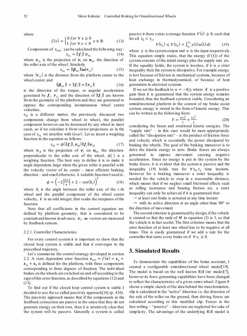
Figure 11 shows linear and angular velocity components of the platform in body coordinates and the value of the 𝑐𝑐𝑖𝑖𝑡𝑡𝑐𝑐𝑡𝑡 function for each wheel vs. time. The brakes were engaged at 4s. A change in the direction of friction forces is well visib le at 5s.
start of braking
stop
𝑓𝑓𝑟𝑟𝑐𝑐𝑡𝑡𝑖𝑖𝑣𝑣𝑒𝑒 𝑥𝑥
𝑓𝑓𝑝𝑝𝑟𝑟𝑐𝑐𝑐𝑐𝑖𝑖𝑣𝑣𝑒𝑒
𝒇𝒇𝒚𝒚
𝒇𝒇𝑥𝑥
𝑦𝑦
54 Viktor Kálmán: Controlled Braking for Omnidirectional Wheels
Figure 11. Platform velocity components in body reference and 𝑐𝑐𝑖𝑖𝑡𝑡𝑐𝑐𝑡𝑡 function for a straight line braking maneuver. Mecanum platform, unassisted case
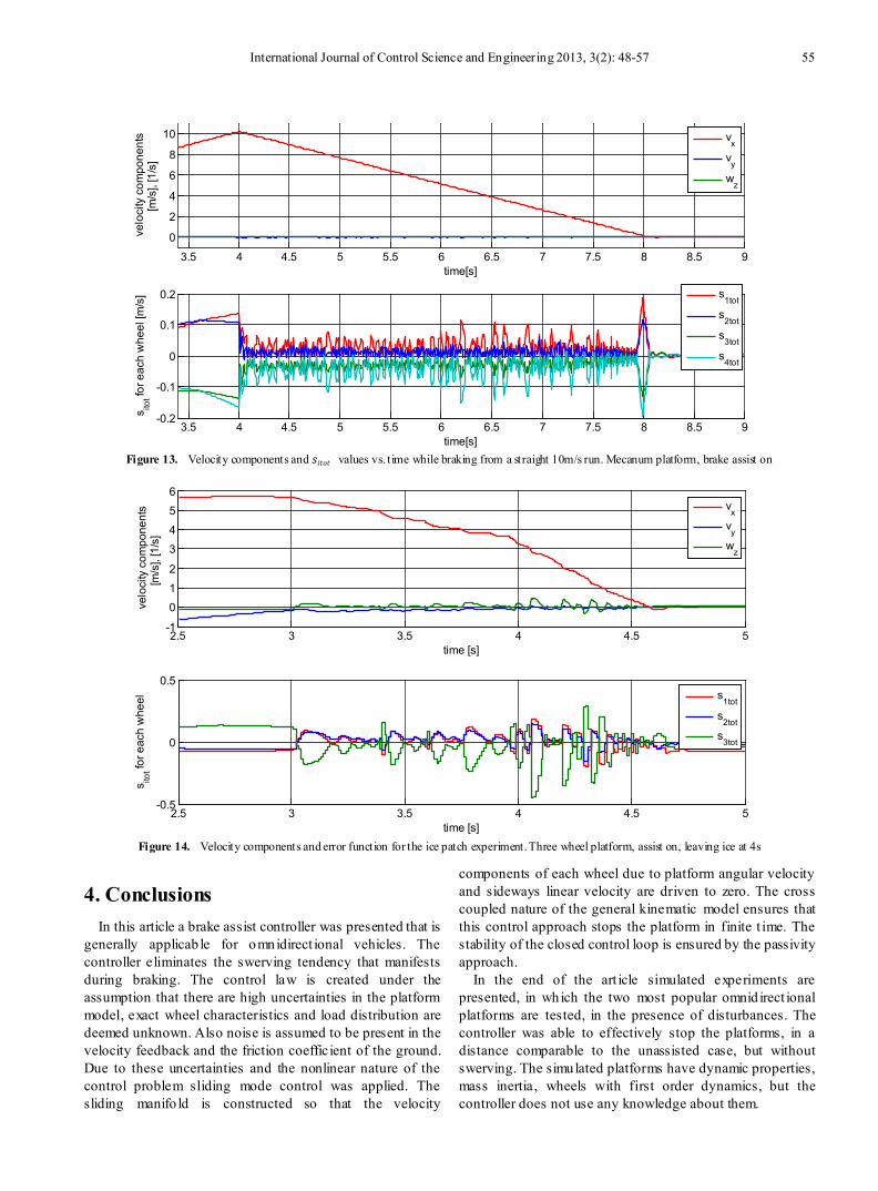
Figure 13 shows the same quantities for the same experiment, this time with the brake assist activated. It is worth noting that during the braking process the platform only has a velocity component in the x direction the y component and the angular velocity are negligib le.
3.2. Disturbance Rejection and Practical Considerations
While in theory ideal sliding mode can be reached by applying infin ite actuator frequency, in reality that is impossible to achieve. In practice actuator frequency needs to be sufficiently high compared to time constants of the controlled plant.
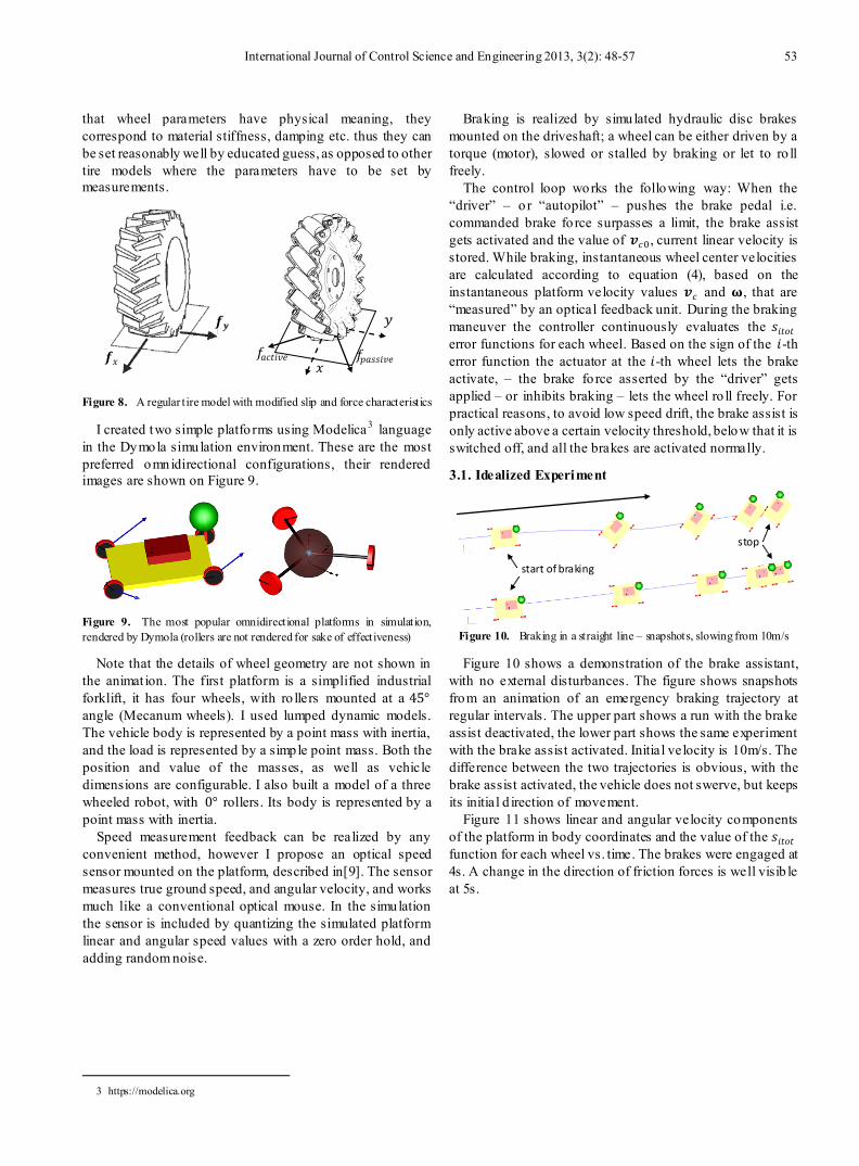
Figure 12. Disturbance rejection: snapshots of braking on “ice”. Bright platform – assist on, dark platform – assist off
To model the effect of limited actuator frequency I quantized the update of feedback values and kept the velocity values constant for 10ms. Because of this the value of the 𝒔𝒔𝑡𝑡𝑐𝑐𝑡𝑡 function did not change, keeping the actuator state constant, limit ing feedback speed.
To introduce unstructured disturbance I created a patch on the ground with a s maller friction coefficient and made the vehicle brake with some of its wheels on the “icy patch” and the others on regular ground. I also added some noise to the feedback. Noise is simulated by a uniform distribution centered around the real value with an adjustable percentage limit 4 . It can be set independently for the linear and the angular velocities. Also an offset can be incorporated in the signal.
𝒗𝒗�𝑐𝑐 ∈ [(1 − 𝑟𝑟)𝒗𝒗𝑐𝑐 + 𝒗𝒗𝑐𝑐 , (1 + 𝑟𝑟)𝒗𝒗𝑐𝑐 + 𝒗𝒗𝑐𝑐 ] (21) where 𝒗𝒗�𝑐𝑐 is the noisy linear velocity signal, 𝑟𝑟 is a percentage value, and 𝒗𝒗𝑐𝑐 = �𝑣𝑣𝑐𝑐𝑥𝑥 , 𝑣𝑣𝑐𝑐𝑦𝑦 � is an o ffset. Similarly
𝛚𝛚� ∈ [(1 − p)𝛚𝛚 +𝝎𝝎𝑐𝑐 , (1 + 𝑟𝑟)𝛚𝛚 + 𝝎𝝎𝑐𝑐 ] (22) where 𝛚𝛚� is the noisy angular velocity measurement p is a percent value and 𝝎𝝎𝑐𝑐 is an offset. Figure 12 shows overlaid snapshots of an assisted and non-assisted braking maneuver on an ice patch, with a noisy feedback signal, where 𝒗𝒗𝑐𝑐 = {0.01, 0.01}, 𝑟𝑟 = 0.15, 𝝎𝝎𝑐𝑐 = {0,0,0.05} , 𝑝𝑝 = 0.15 . The brighter colored platform had an active brake assist with a noisy feedback, the dark platfo rm had no brake assist.
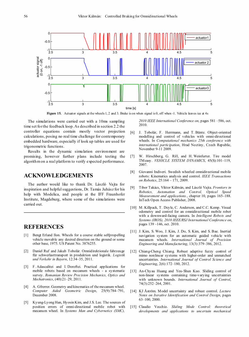
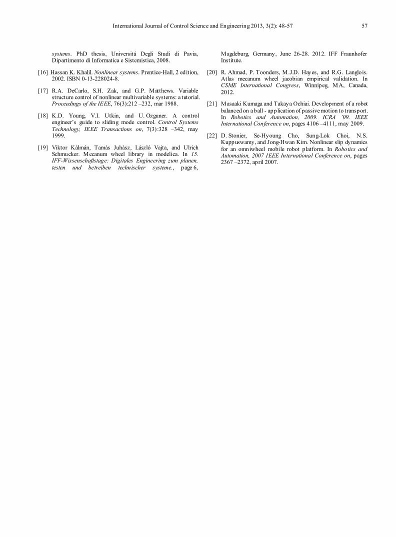
The experiment demonstrates that the controller tolerates the disturbances really well, as opposed to the unassisted case it does not swerve but keeps its orientation. As a disadvantage it can be noted that braking distance is a little longer in the assisted case, due to adaptation of brake forces to the lower friction on all wheels. Error and velocity signals are shown on Figure 14. Actuator signals are shown on Figure 15, for the three wheels in the order marked on Figure 13. The frequency at which the actuators work is well within the capabilit ies of hydraulic valves used in contemporary ABS systems.
4 Uniform distribution might not be the best simulation of sensor noise, however my purpose here is to demonstrate disturbance rejection of the controller.
3.5 4 4.5 5 5.5 6 6.5 7 7.5 8 8.5 9-5
0
5
10
time[s]
velo
city
com
pone
nts
[m/s
], [1
/s]
v
x
vy
wz
3.5 4 4.5 5 5.5 6 6.5 7 7.5 8 8.5 9
-5
0
5
time[s]
s itot fo
r eac
h w
heel
[m/s
]
s
1tot
s2tot
s3tot
s4tot
𝜇𝜇 = 0.2
𝜇𝜇 = 0.8
assisted
ICE
All brakes on at this instant
1
2 3
STOP
unassisted
International Journal of Control Science and Engineering 2013, 3(2): 48-57 55
Figure 13. Velocity components and 𝑐𝑐𝑖𝑖𝑡𝑡𝑐𝑐𝑡𝑡 values vs. t ime while braking from a straight 10m/s run. Mecanum platform, brake assist on
Figure 14. Velocity components and error function for the ice patch experiment. Three wheel platform, assist on, leaving ice at 4s
4. Conclusions In this article a brake assist controller was presented that is
generally applicab le for omnidirect ional vehicles. The controller eliminates the swerving tendency that manifests during braking. The control law is created under the assumption that there are high uncertainties in the platform model, exact wheel characteristics and load distribution are deemed unknown. Also noise is assumed to be present in the velocity feedback and the friction coefficient of the ground. Due to these uncertainties and the nonlinear nature of the control problem sliding mode control was applied. The sliding manifo ld is constructed so that the velocity
components of each wheel due to platform angular velocity and sideways linear velocity are driven to zero. The cross coupled nature of the general kinematic model ensures that this control approach stops the platform in finite t ime. The stability of the closed control loop is ensured by the passivity approach.
In the end of the art icle simulated experiments are presented, in which the two most popular omnid irect ional platforms are tested, in the presence of disturbances. The controller was able to effectively stop the platforms, in a distance comparable to the unassisted case, but without swerving. The simulated platforms have dynamic properties, mass inertia , wheels with first order dynamics, but the controller does not use any knowledge about them.
3.5 4 4.5 5 5.5 6 6.5 7 7.5 8 8.5 9
0
2
4
6
8
10
time[s]
velo
city
com
pone
nts
[m/s
], [1
/s]
v
x
vy
wz
3.5 4 4.5 5 5.5 6 6.5 7 7.5 8 8.5 9-0.2
-0.1
0
0.1
0.2
time[s]
s itot fo
r eac
h w
heel
[m/s
]
s1tot
s2tot
s3tot
s4tot
2.5 3 3.5 4 4.5 5-1
0
1
2
3
4
5
6
time [s]
velo
city
com
pone
nts
[m/s
], [1
/s]
v
x
vy
wz
2.5 3 3.5 4 4.5 5-0.5
0
0.5
time [s]
s itot fo
r eac
h w
heel
s
1tot
s2tot
s3tot
56 Viktor Kálmán: Controlled Braking for Omnidirectional Wheels
Figure 15. Actuator signals at the wheels 1, 2 and 3. Brake is on when signal is 0, off when -1. Vehicle leaves ice at 4s
The simulat ions were carried out with a 10ms sampling time set fo r the feedback loop. As described in section 2.2 the controller equations contain mostly vector projection calculations, posing no real time challenge for contemporary embedded hardware, especially if look up tables are used for trigonometric functions.
Results in the dynamic simulation environment are promising, however further p lans include testing the algorithm on a real platform to verify expected performance.
ACKNOWLEDGEMENTS The author would like to thank Dr. László Vajta for
inspiration and helpful suggestions, Dr. Tamás Juhász for his help with Modelica, and people at the IFF Fraunhofer Institute, Magdeburg, where some of the simulations were carried out.
REFERENCES [1] Bengt Erland Ilon. Wheels for a course stable selfpropelling
vehicle movable any desired direction on the ground or some other base, 1975. US Patent No. 3876255.
[2] Daniel Ruf and Jakub Tobolár. Omnidirektionale fahrzeuge für schwerlasttransport in produktion und logistik. Logistik und Verkehr in Bayern, 12:34–35, 2011.
[3] F. Adascalitei and I. Doroftei. Practical applications for mobile robots based on mecanum wheels - a systematic survey. Romanian Review Precision Mechanics, Optics and Mechatronics, (40):21–29, 2011.
[4] A. Gfrerrer. Geometry and kinematics of the mecanum wheel. Computer Aided Geometric Design, 25(9):784–791, December 2008.
[5] Kyung-Lyong Han, Hyosin Kim, and J.S. Lee. The sources of position errors of omni-directional mobile robot with mecanum wheel. In Systems Man and Cybernetics (SMC),
2010 IEEE International Conference on, pages 581 –586, oct. 2010.
[6] J. Tobolár, F. Herrmann, and T. Bünte. Object-oriented modelling and control of vehicles with omni-directional wheels. In Computational mechanics 25th conference with international participation, Hrad Nectiny, Czech Republic, November 9-11 2009.
[7] W. Hirschberg, G. Rill, and H. Weinfurter. Tire model TMeasy. VEHICLE SYSTEM DYNAMICS, 45(S):101–119, 2007.
[8] Giovanni Indiveri. Swedish wheeled omnidirectional mobile robots: Kinematics analysis and control. IEEE Transactions on Robotics, 25:164 – 171, 2009.
[9] Tibor Takács, Viktor Kálmán, and László Vajta. Frontiers in Robotics, Automation and Control, Optical Speed Measurement and applications., chapter 10, pages 165–188. InTech Open Access Publisher, 2008.
[10] M. Killpack, T. Deyle, C. Anderson, and C.C. Kemp. Visual odometry and control for an omnidirectional mobile robot with a downward-facing camera. In Intelligent Robots and Systems (IROS), 2010 IEEE/RSJ International Conference on, pages 139 –146, oct. 2010.
[11] J. Kim, S. Woo, J. Kim, J. Do, S. Kim, and S. Bae. Inertial navigation system for an automatic guided vehicle with mecanum wheels. International Journal of Precision Engineering and Manufacturing, 13(3):379–386, 2012.
[12] Chiang-Cheng Chiang. Robust adaptive fuzzy control of mimo nonlinear systems with higher-order and unmatched uncertainties. International Journal of Control Science and Engineering, 2(6):172–180, 2012.
[13] An-Chyau Huang and Yeu-Shun Kuo. Sliding control of non-linear systems containing time-varying uncertainties with unknown bounds. International Journal of Control, 74(3):252–264, 2001.
[14] KJ Åström. Model uncertainty and robust control. Lecture Notes on Iterative Identification and Control Design, pages 63–100, 2000.
[15] Claudio Vecchio. Sliding Mode Control: theoretical developments and applications to uncertain mechanical
2.5 3 3.5 4 4.5 5-1
-0.5
0
actuator1
2.5 3 3.5 4 4.5 5-1
-0.5
0
actu
ator
sig
nal
(0 o
n, -1
off)
actuator 2
2.5 3 3.5 4 4.5 5-1
-0.5
0
time [s]
actuator3
International Journal of Control Science and Engineering 2013, 3(2): 48-57 57
systems. PhD thesis, Universitá Degli Studi di Pavia, Dipartimento di Informatica e Sistemistica, 2008.
[16] Hassan K. Khalil. Nonlinear systems. Prentice-Hall, 2 edition, 2002. ISBN 0-13-228024-8.
[17] R.A. DeCarlo, S.H. Zak, and G.P. Matthews. Variable structure control of nonlinear multivariable systems: a tutorial. Proceedings of the IEEE, 76(3):212 –232, mar 1988.
[18] K.D. Young, V.I. Utkin, and U. Ozguner. A control engineer’s guide to sliding mode control. Control Systems Technology, IEEE Transactions on, 7(3):328 –342, may 1999.
[19] Viktor Kálmán, Tamás Juhász, László Vajta, and Ulrich Schmucker. Mecanum wheel library in modelica. In 15. IFF-Wissenschaftstage: Digitales Engineering zum planen, testen und betreiben technischer systeme., page 6,
Magdeburg, Germany, June 26-28. 2012. IFF Fraunhofer Institute.
[20] R. Ahmad, P. Toonders, M.J.D. Hayes, and R.G. Langlois. Atlas mecanum wheel jacobian empirical validation. In CSME International Congress, Winnipeg, MA, Canada, 2012.
[21] Masaaki Kumaga and Takaya Ochiai. Development of a robot balanced on a ball - application of passive motion to transport. In Robotics and Automation, 2009. ICRA ’09. IEEE International Conference on, pages 4106 –4111, may 2009.
[22] D. Stonier, Se-Hyoung Cho, Sung-Lok Choi, N.S. Kuppuswamy, and Jong-Hwan Kim. Nonlinear slip dynamics for an omniwheel mobile robot platform. In Robotics and Automation, 2007 IEEE International Conference on, pages 2367 –2372, april 2007.


![REGENERATIVE BRAKING SYSTEM IN ELECTRIC VEHICLES · REGENERATIVE BRAKING SYSTEM IN ELECTRIC VEHICLES ... REGENERATIVE BRAKING SYSTEM ... Regenerative action during braking[9].](https://static.fdocuments.us/doc/165x107/5adccef67f8b9a1a088c7cf0/regenerative-braking-system-in-electric-vehicles-braking-system-in-electric-vehicles.jpg)