Control Systems Design, SC4026 - TU Delftaabate/2010sc4026/sc4026_lec1.pdf · Control Systems...
22
Control Systems Design, SC4026 SC4026 Fall 2010, dr. A. Abate, DCSC, TU Delft
Transcript of Control Systems Design, SC4026 - TU Delftaabate/2010sc4026/sc4026_lec1.pdf · Control Systems...

Control Systems Design, SC4026
SC4026 Fall 2010, dr. A. Abate, DCSC, TU Delft
Lecture 1
• The concept of feedback
• The concept of “model” in systems engineering: state-space models
• The role of a controller
SC4026 Fall 2010, dr. A. Abate, DCSC, TU Delft 1
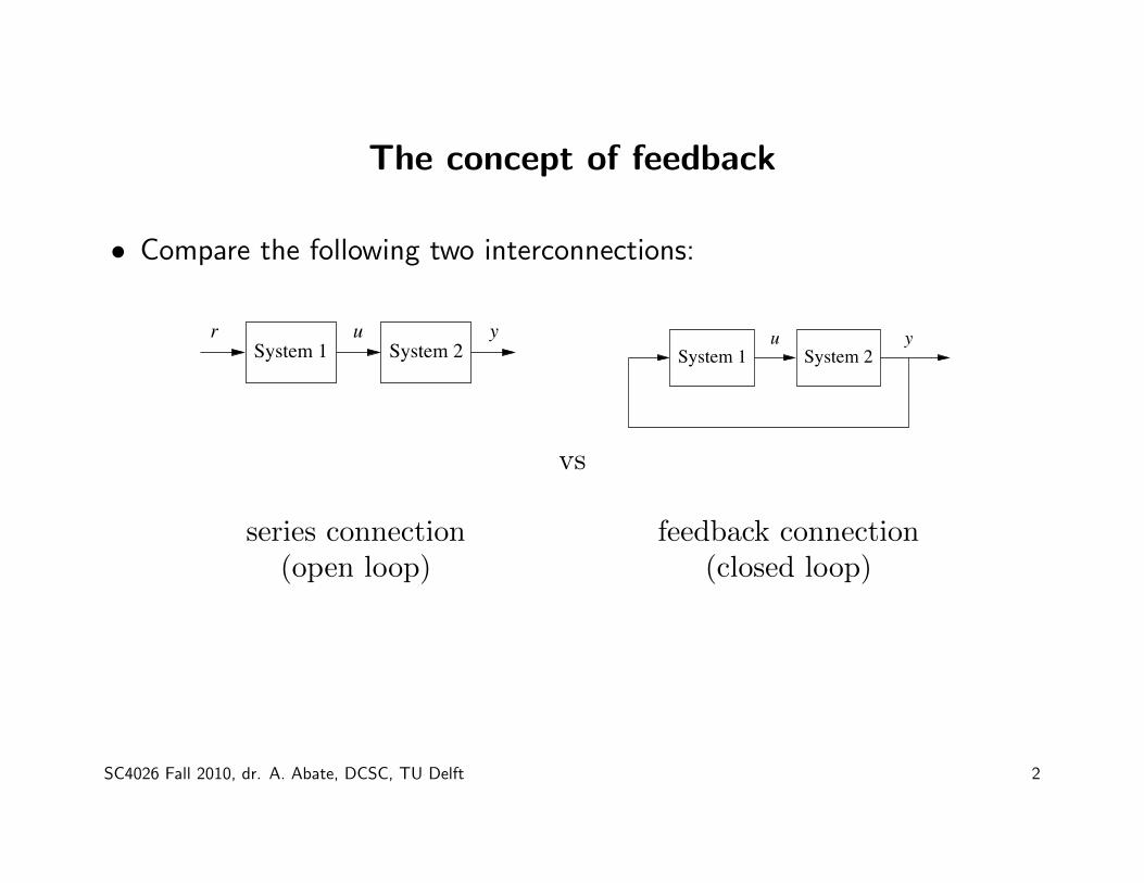
The concept of feedback
• Compare the following two interconnections:
Chapter OneIntroduction
Feedback is a central feature of life. The process of feedback governs how we grow, respond
to stress and challenge, and regulate factors such as body temperature, blood pressure and
cholesterol level. The mechanisms operate at every level, from the interaction of proteins in
cells to the interaction of organisms in complex ecologies.
M. B. Hoagland and B. Dodson, The Way Life Works, 1995 [HD95].
In this chapter we provide an introduction to the basic concept of feedback and
the related engineering discipline of control.We focus on both historical and current
examples, with the intention of providing the context for current tools in feedback
and control. Much of the material in this chapter is adapted from [Mur03], and
the authors gratefully acknowledge the contributions of Roger Brockett and Gunter
Stein to portions of this chapter.
1.1 What Is Feedback?
Adynamical system is a systemwhose behavior changes over time, often in response
to external stimulation or forcing. The term feedback refers to a situation in which
two (or more) dynamical systems are connected together such that each system
influences the other and their dynamics are thus strongly coupled. Simple causal
reasoning about a feedback system is difficult because the first system influences
the second and the second system influences the first, leading to a circular argument.
Thismakes reasoning based on cause and effect tricky, and it is necessary to analyze
the systemas awhole.Aconsequence of this is that the behavior of feedback systems
is often counterintuitive, and it is therefore necessary to resort to formal methods
to understand them.
Figure 1.1 illustrates in block diagram form the idea of feedback. We often use
uSystem 2System 1
y
(a) Closed loop
ySystem 2System 1
ur
(b) Open loop
Figure 1.1: Open and closed loop systems. (a) The output of system 1 is used as the input of
system 2, and the output of system 2 becomes the input of system 1, creating a closed loop
system. (b) The interconnection between system 2 and system 1 is removed, and the system
is said to be open loop.
vs
series connection(open loop)
feedback connection(closed loop)
SC4026 Fall 2010, dr. A. Abate, DCSC, TU Delft 2
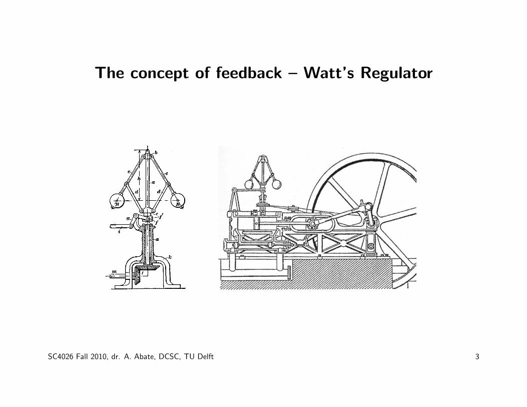
The concept of feedback – Watt’s Regulator
2 CHAPTER 1. INTRODUCTION
Figure 1.2: The centrifugal governor and the steam engine. The centrifugal governor on the
left consists of a set of flyballs that spread apart as the speed of the engine increases. The
steam engine on the right uses a centrifugal governor (above and to the left of the flywheel)
to regulate its speed. (Credit: Machine a Vapeur Horizontale de Philip Taylor [1828].)
the terms open loop and closed loop when referring to such systems. A system
is said to be a closed loop system if the systems are interconnected in a cycle, as
shown in Figure 1.1a. If we break the interconnection, we refer to the configuration
as an open loop system, as shown in Figure 1.1b.
As the quote at the beginning of this chapter illustrates, a major source of exam-
ples of feedback systems is biology. Biological systems make use of feedback in an
extraordinary number of ways, on scales ranging from molecules to cells to organ-
isms to ecosystems. One example is the regulation of glucose in the bloodstream
through the production of insulin and glucagon by the pancreas. The body attempts
to maintain a constant concentration of glucose, which is used by the body’s cells
to produce energy. When glucose levels rise (after eating a meal, for example), the
hormone insulin is released and causes the body to store excess glucose in the liver.
When glucose levels are low, the pancreas secretes the hormone glucagon, which
has the opposite effect. Referring to Figure 1.1, we can view the liver as system 1
and the pancreas as system 2. The output from the liver is the glucose concentration
in the blood, and the output from the pancreas is the amount of insulin or glucagon
produced. The interplay between insulin and glucagon secretions throughout the
day helps to keep the blood-glucose concentration constant, at about 90 mg per
100 mL of blood.
An early engineering example of a feedback system is a centrifugal governor,
in which the shaft of a steam engine is connected to a flyball mechanism that is
itself connected to the throttle of the steam engine, as illustrated in Figure 1.2. The
system is designed so that as the speed of the engine increases (perhaps because of a
lessening of the load on the engine), the flyballs spread apart and a linkage causes the
throttle on the steam engine to be closed. This in turn slows down the engine, which
causes the flyballs to come back together. We can model this system as a closed
loop system by taking system 1 as the steam engine and system 2 as the governor.
SC4026 Fall 2010, dr. A. Abate, DCSC, TU Delft 3
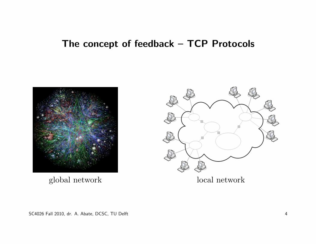
The concept of feedback – TCP Protocols
global network local network
SC4026 Fall 2010, dr. A. Abate, DCSC, TU Delft 4
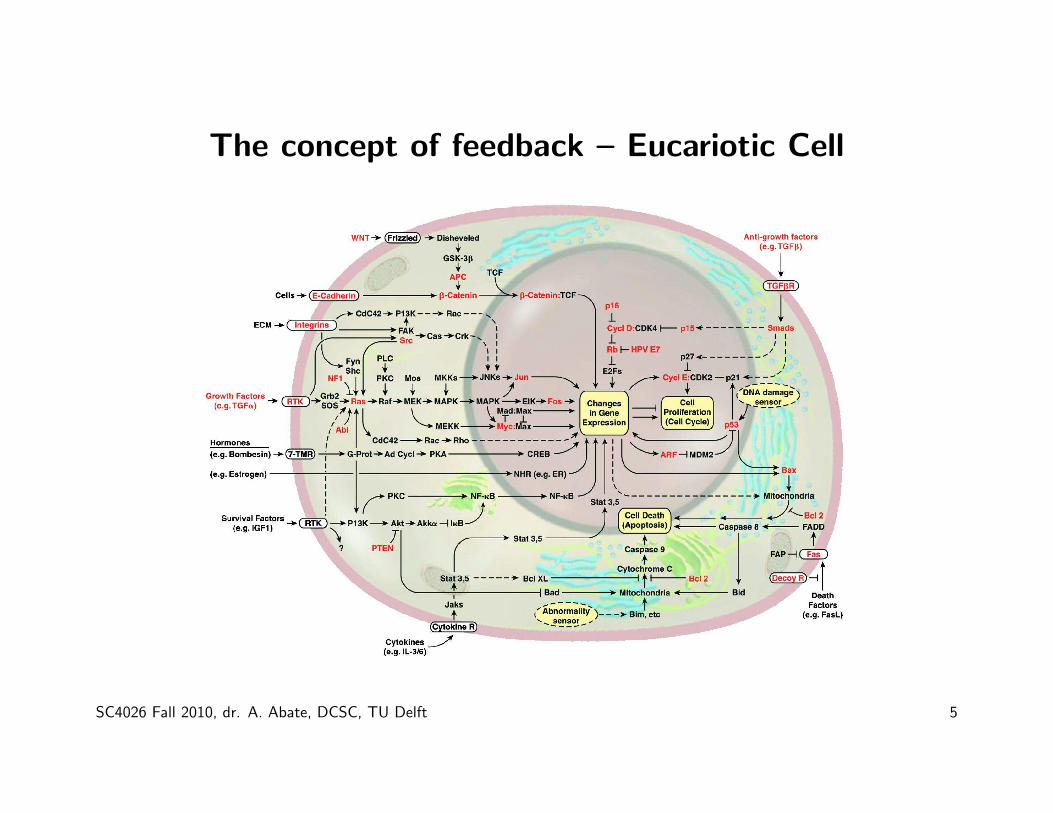
The concept of feedback – Eucariotic Cell16 CHAPTER 1. INTRODUCTION
Figure 1.12: The wiring diagram of the growth-signaling circuitry of the mammalian
cell [HW00]. The major pathways that are thought to play a role in cancer are indicated
in the diagram. Lines represent interactions between genes and proteins in the cell. Lines
ending in arrowheads indicate activation of the given gene or pathway; lines ending in a
T-shaped head indicate repression. (Used with permission of Elsevier Ltd. and the authors.)
nity is the science of reverse (and eventually forward) engineering of biological
control networks such as the one shown in Figure 1.12. There are a wide variety
of biological phenomena that provide a rich source of examples of control, includ-
ing gene regulation and signal transduction; hormonal, immunological and cardio-
vascular feedback mechanisms; muscular control and locomotion; active sensing,
vision and proprioception; attention and consciousness; and population dynamics
and epidemics. Each of these (and many more) provide opportunities to figure out
what works, how it works, and what we can do to affect it.
One interesting feature of biological systems is the frequent use of positive feed-
back to shape the dynamics of the system. Positive feedback can be used to create
switchlike behavior through autoregulation of a gene, and to create oscillations such
as those present in the cell cycle, central pattern generators or circadian rhythm.
Ecosystems. In contrast to individual cells and organisms, emergent properties
of aggregations and ecosystems inherently reflect selection mechanisms that act on
multiple levels, and primarily on scales well below that of the system as a whole.
Because ecosystems are complex, multiscale dynamical systems, they provide a
broad range of new challenges for the modeling and analysis of feedback systems.
Recent experience in applying tools fromcontrol and dynamical systems to bacterial
networks suggests that much of the complexity of these networks is due to the
presence of multiple layers of feedback loops that provide robust functionality
SC4026 Fall 2010, dr. A. Abate, DCSC, TU Delft 5
The concept of feedback – Predator/Prey Environments2.2. STATE SPACE MODELS 39
1845
160
140
120
100
80
60
40
20
1855 1865 1875 1885 1895
HareLynx
1905 1915 1925 1935
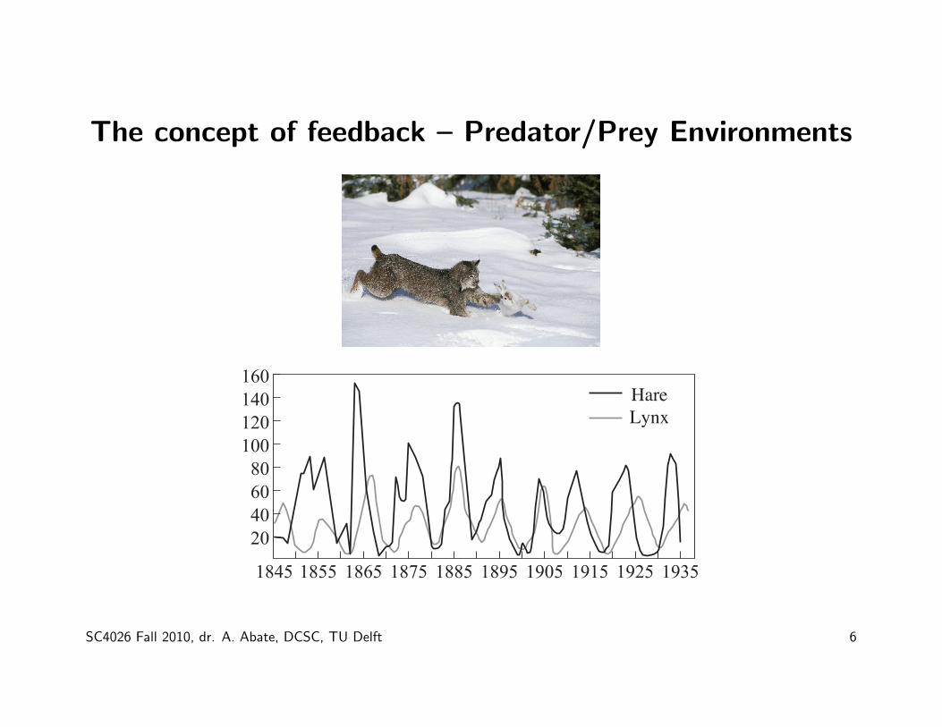
Figure 2.6: Predator versus prey. The photograph on the left shows a Canadian lynx and
a snowshoe hare, the lynx’s primary prey. The graph on the right shows the populations of
hares and lynxes between 1845 and 1935 in a section of the Canadian Rockies [Mac37]. The
data were collected on an annual basis over a period of 90 years. (Photograph copyright Tom
and Pat Leeson.)
discrete-time index (e.g., the month number), we can write
H [k + 1] = H [k]+ br (u)H [k]! aL[k]H [k],
L[k + 1] = L[k]+ cL[k]H [k]! d f L[k],(2.13)
where br (u) is the hare birth rate per unit period and as a function of the foodsupply u, d f is the lynx mortality rate and a and c are the interaction coefficients.
The interaction term aL[k]H [k] models the rate of predation, which is assumed
to be proportional to the rate at which predators and prey meet and is hence given
by the product of the population sizes. The interaction term cL[k]H [k] in the
lynx dynamics has a similar form and represents the rate of growth of the lynx
population. This model makes many simplifying assumptions—such as the fact
that hares decrease in number only through predation by lynxes—but it often is
sufficient to answer basic questions about the system.
To illustrate the use of this system, we can compute the number of lynxes and
hares at each time point from some initial population. This is done by starting with
x[0] = (H0, L0) and then using equation (2.13) to compute the populations inthe following period. By iterating this procedure, we can generate the population
over time. The output of this process for a specific choice of parameters and initial
conditions is shown in Figure 2.7. While the details of the simulation are different
from the experimental data (to be expected given the simplicity of our assumptions),
we see qualitatively similar trends and hence we can use the model to help explore
the dynamics of the system. "Example 2.4 E-mail server
The IBM Lotus server is an collaborative software system that administers users’
e-mail, documents and notes. Client machines interact with end users to provide
access to data and applications. The server also handles other administrative tasks.
In the early development of the system it was observed that the performance was
poor when the central processing unit (CPU) was overloaded because of too many
service requests, and mechanisms to control the load were therefore introduced.
The interaction between the client and the server is in the form of remote pro-
2.2. STATE SPACE MODELS 39
1845
160
140
120
100
80
60
40
20
1855 1865 1875 1885 1895
HareLynx
1905 1915 1925 1935
Figure 2.6: Predator versus prey. The photograph on the left shows a Canadian lynx and
a snowshoe hare, the lynx’s primary prey. The graph on the right shows the populations of
hares and lynxes between 1845 and 1935 in a section of the Canadian Rockies [Mac37]. The
data were collected on an annual basis over a period of 90 years. (Photograph copyright Tom
and Pat Leeson.)
discrete-time index (e.g., the month number), we can write
H [k + 1] = H [k]+ br (u)H [k]! aL[k]H [k],
L[k + 1] = L[k]+ cL[k]H [k]! d f L[k],(2.13)
where br (u) is the hare birth rate per unit period and as a function of the foodsupply u, d f is the lynx mortality rate and a and c are the interaction coefficients.
The interaction term aL[k]H [k] models the rate of predation, which is assumed
to be proportional to the rate at which predators and prey meet and is hence given
by the product of the population sizes. The interaction term cL[k]H [k] in the
lynx dynamics has a similar form and represents the rate of growth of the lynx
population. This model makes many simplifying assumptions—such as the fact
that hares decrease in number only through predation by lynxes—but it often is
sufficient to answer basic questions about the system.
To illustrate the use of this system, we can compute the number of lynxes and
hares at each time point from some initial population. This is done by starting with
x[0] = (H0, L0) and then using equation (2.13) to compute the populations inthe following period. By iterating this procedure, we can generate the population
over time. The output of this process for a specific choice of parameters and initial
conditions is shown in Figure 2.7. While the details of the simulation are different
from the experimental data (to be expected given the simplicity of our assumptions),
we see qualitatively similar trends and hence we can use the model to help explore
the dynamics of the system. "Example 2.4 E-mail server
The IBM Lotus server is an collaborative software system that administers users’
e-mail, documents and notes. Client machines interact with end users to provide
access to data and applications. The server also handles other administrative tasks.
In the early development of the system it was observed that the performance was
poor when the central processing unit (CPU) was overloaded because of too many
service requests, and mechanisms to control the load were therefore introduced.
The interaction between the client and the server is in the form of remote pro-
SC4026 Fall 2010, dr. A. Abate, DCSC, TU Delft 6
The use of Mathematical Models
• Objective: quantitative description of a system
• How to construct a model?
– physics-based model (conservation laws, physical geometry anddimensions)
– models based on known interactions and properties (e.g.:energy-based models, stoichiometric models)
– Models from experiments (data driven): measurement of modelproperties and use of fitting, use of transfer functions
(SC4032: Physical Modelling for Systems and Control)
SC4026 Fall 2010, dr. A. Abate, DCSC, TU Delft 7

(SC4110: Systems Identification)(SC4040: Filtering & Identification)
SC4026 Fall 2010, dr. A. Abate, DCSC, TU Delft 8
State-space Models: a First Example
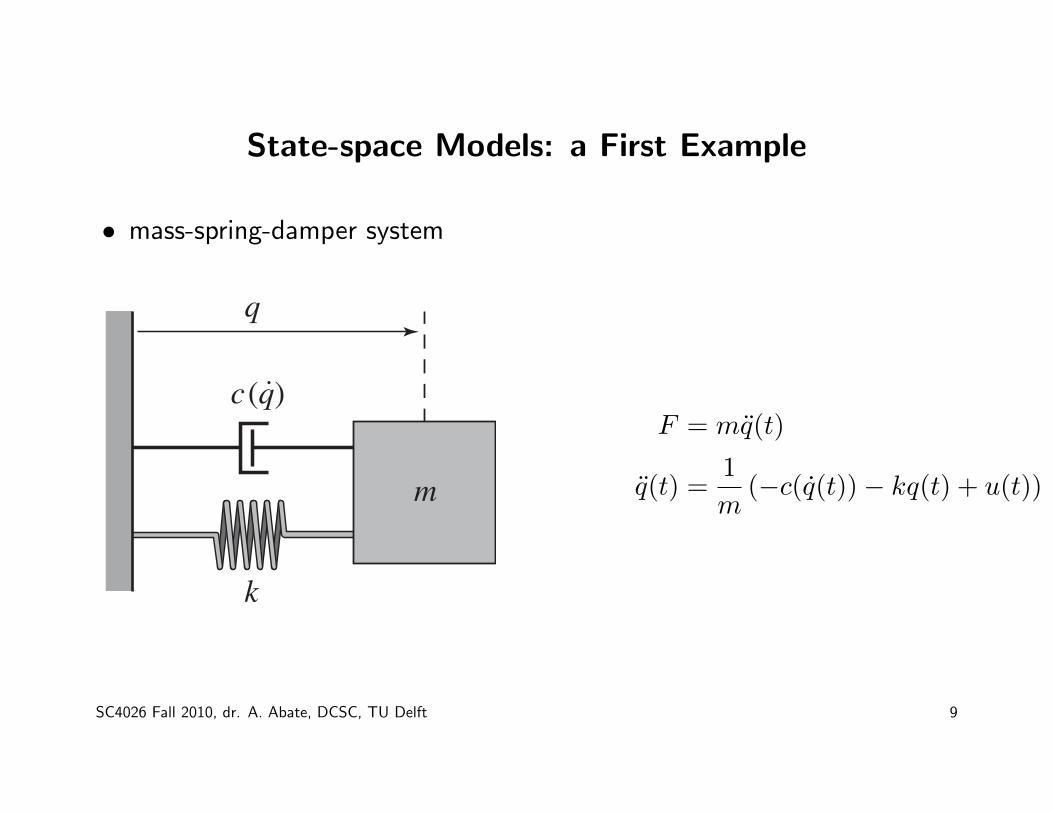
• mass-spring-damper system28 CHAPTER 2. SYSTEM MODELING
c (q)
q
m
k
Figure 2.1: Spring–mass systemwith nonlinear damping. The position of themass is denoted
by q , with q = 0 corresponding to the rest position of the spring. The forces on the mass are
generated by a linear spring with spring constant k and a damper with force dependent on the
velocity q .
The Heritage of Mechanics
The study of dynamics originated in attempts to describe planetary motion. The
basis was detailed observations of the planets by Tycho Brahe and the results of
Kepler, who found empirically that the orbits of the planets could be well described
by ellipses. Newton embarked on an ambitious program to try to explain why the
planets move in ellipses, and he found that the motion could be explained by his
law of gravitation and the formula stating that force equals mass times acceleration.
In the process he also invented calculus and differential equations.
One of the triumphs of Newton’s mechanics was the observation that the motion
of the planets could be predicted based on the current positions and velocities of
all planets. It was not necessary to know the past motion. The state of a dynamical
system is a collection of variables that completely characterizes the motion of a
system for the purpose of predicting future motion. For a system of planets the
state is simply the positions and the velocities of the planets. We call the set of all
possible states the state space.
A common class of mathematical models for dynamical systems is ordinary
differential equations (ODEs). In mechanics, one of the simplest such differential
equations is that of a spring–mass system with damping:
mq + c(q) + kq = 0. (2.1)
This system is illustrated in Figure 2.1. The variable q ! R represents the positionof the mass m with respect to its rest position. We use the notation q to denote the
derivative of q with respect to time (i.e., the velocity of the mass) and q to represent
the second derivative (acceleration). The spring is assumed to satisfy Hooke’s law,
which says that the force is proportional to the displacement. The friction element
(damper) is taken as a nonlinear function c(q), which can model effects such asstiction and viscous drag. The position q and velocity q represent the instantaneous
state of the system. We say that this system is a second-order system since the
dynamics depend on the first two derivatives of q.
The evolution of the position and velocity can be described using either a time
plot or a phase portrait, both of which are shown in Figure 2.2. The time plot, on
F = mq(t)
q(t) =1
m(−c(q(t))− kq(t) + u(t))
SC4026 Fall 2010, dr. A. Abate, DCSC, TU Delft 9
State-space Models: a First Example
• State: q(t)
• Input signal: u(t)
• Output signal: y(t) = q(t)
SC4026 Fall 2010, dr. A. Abate, DCSC, TU Delft 10
State-space Models: a First Example
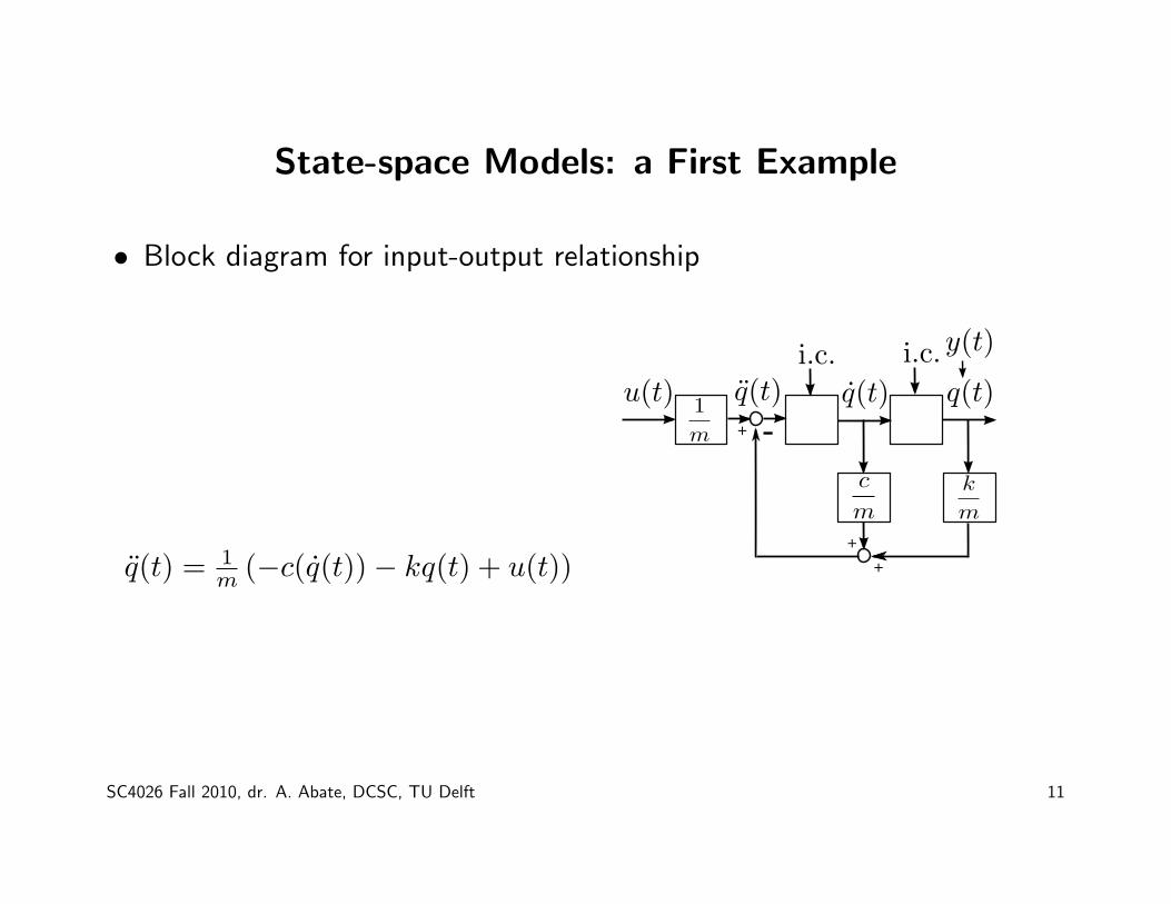
• Block diagram for input-output relationship
q(t) = 1m (−c(q(t))− kq(t) + u(t))
!
!
!
"
################################################################################################################################################
!
!
!
"SC4026 Fall 2010, dr. A. Abate, DCSC, TU Delft 11
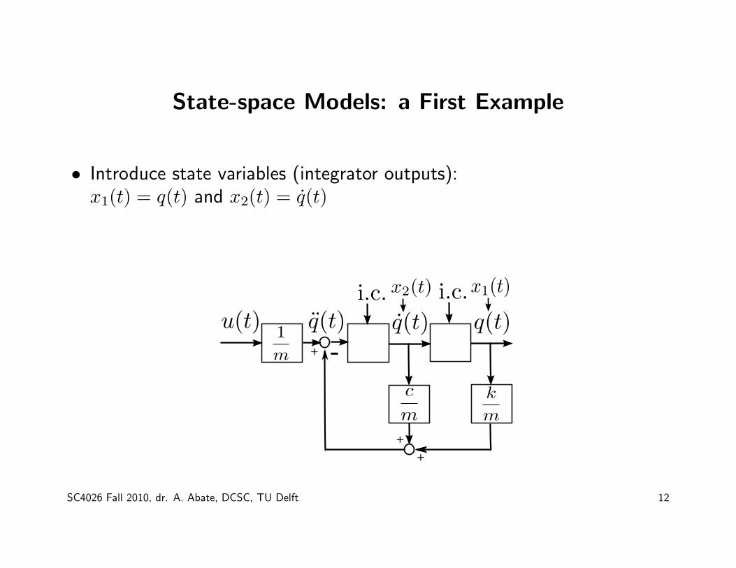
State-space Models: a First Example
• Introduce state variables (integrator outputs):x1(t) = q(t) and x2(t) = q(t)
!
!
!
"
################################################################################################################################################
!
!
!
"
SC4026 Fall 2010, dr. A. Abate, DCSC, TU Delft 12
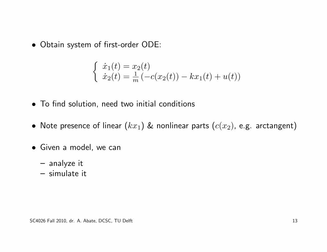
• Obtain system of first-order ODE:{x1(t) = x2(t)x2(t) =
1m (−c(x2(t))− kx1(t) + u(t))
• To find solution, need two initial conditions
• Note presence of linear (kx1) & nonlinear parts (c(x2), e.g. arctangent)
• Given a model, we can
– analyze it– simulate it
SC4026 Fall 2010, dr. A. Abate, DCSC, TU Delft 13
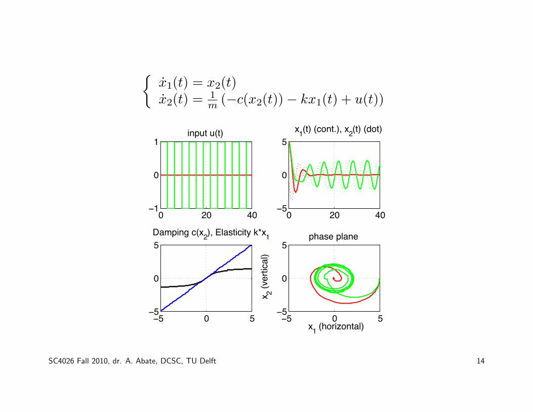
{x1(t) = x2(t)x2(t) =
1m (−c(x2(t))− kx1(t) + u(t))
0 20 40−1
0
1input u(t)
0 20 40−5
0
5x1(t) (cont.), x2(t) (dot)
−5 0 5−5
0
5Damping c(x2), Elasticity k*x1
−5 0 5−5
0
5phase plane
x1 (horizontal)
x 2 (ver
tical
)
SC4026 Fall 2010, dr. A. Abate, DCSC, TU Delft 14
State-space Models: a Second Example
• Predator-prey model (introduced before)
• Now we aim at obtaining a quantitative, abstract simplification of theactual dynamics
• State variables:
– time-dependent population level for the lynxes: l(t), t ≥ 0– and for the hares: h(t), t ≥ 0
• Control Input: hare birth rate b(u), function of food
• Outputs: population levels l(t), h(t)
SC4026 Fall 2010, dr. A. Abate, DCSC, TU Delft 15
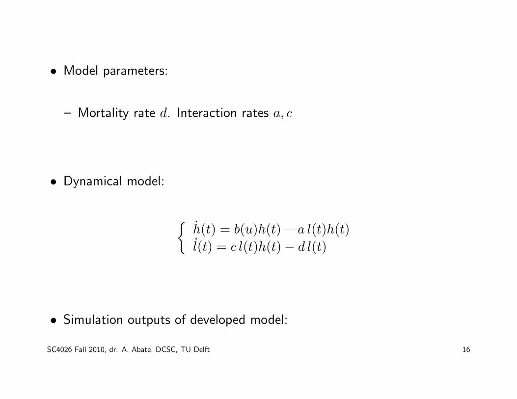
• Model parameters:
– Mortality rate d. Interaction rates a, c
• Dynamical model:
{h(t) = b(u)h(t)− a l(t)h(t)
l(t) = c l(t)h(t)− d l(t)
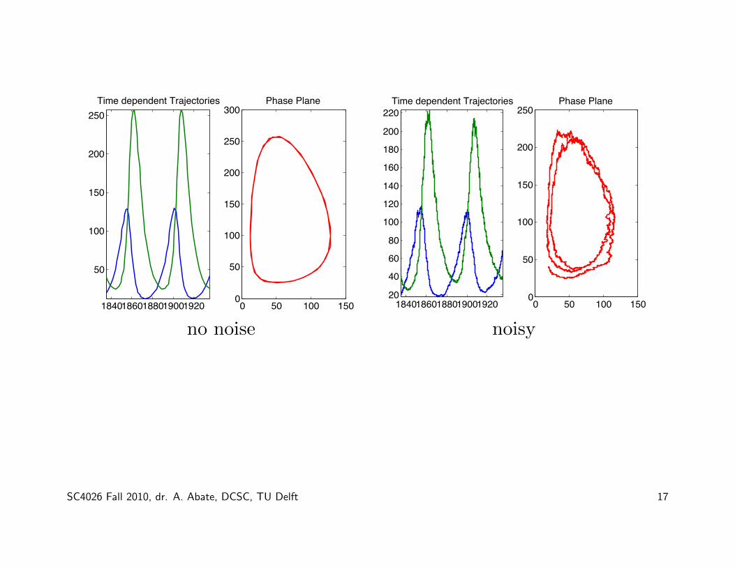
• Simulation outputs of developed model:
SC4026 Fall 2010, dr. A. Abate, DCSC, TU Delft 16
18401860188019001920
50
100
150
200
250Time dependent Trajectories
0 50 100 1500
50
100
150
200
250
300Phase Plane
1840186018801900192020
40
60
80
100
120
140
160
180
200
220Time dependent Trajectories
0 50 100 1500
50
100
150
200
250Phase Plane
no noise noisy
SC4026 Fall 2010, dr. A. Abate, DCSC, TU Delft 17
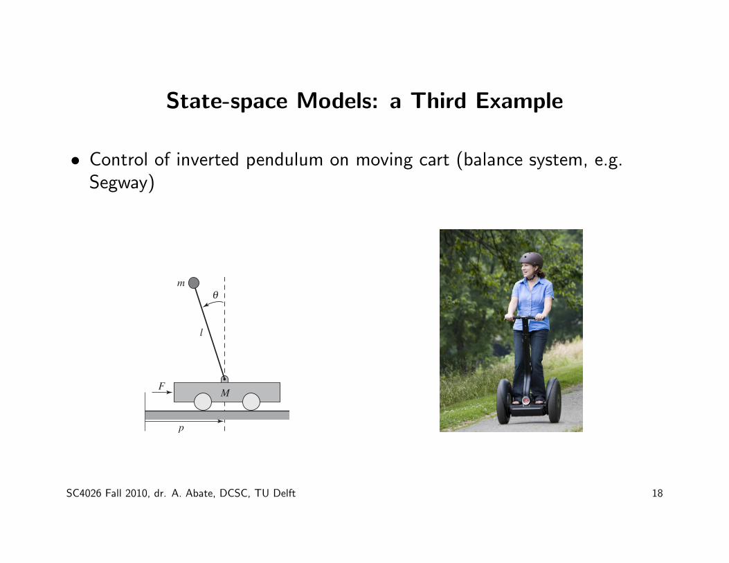
State-space Models: a Third Example
• Control of inverted pendulum on moving cart (balance system, e.g.Segway)
36 CHAPTER 2. SYSTEM MODELING
(a) Segway (b) Saturn rocket
MF
p
!m
l
(c) Cart–pendulum system
Figure 2.5: Balance systems. (a) Segway Personal Transporter, (b) Saturn rocket and (c)
inverted pendulum on a cart. Each of these examples uses forces at the bottom of the system
to keep it upright.
Balance systems are a generalization of the spring–mass system we saw earlier.
We can write the dynamics for a mechanical system in the general form
M(q)q + C(q, q) + K (q) = B(q)u,
where M(q) is the inertia matrix for the system, C(q, q) represents the Coriolisforces as well as the damping, K (q) gives the forces due to potential energy andB(q) describes how the external applied forces couple into the dynamics. The
specific form of the equations can be derived using Newtonian mechanics. Note
that each of the terms depends on the configuration of the system q and that these
terms are often nonlinear in the configuration variables.
Figure 2.5c shows a simplified diagram for a balance system consisting of an
inverted pendulum on a cart. To model this system, we choose state variables that
represent the position and velocity of the base of the system, p and p, and the angle
and angular rate of the structure above the base, ! and ! . We let F represent theforce applied at the base of the system, assumed to be in the horizontal direction
(aligned with p), and choose the position and angle of the system as outputs. With
this set of definitions, the dynamics of the system can be computed usingNewtonian
mechanics and have the form!""# (M + m) !ml cos !
!ml cos ! (J + ml2)
$""%
!""# p
!
$""% +
!""#c p + ml sin ! !2
" ! ! mgl sin !
$""% =
!""#F
0
$""% , (2.9)
where M is the mass of the base,m and J are the mass and moment of inertia of the
system to be balanced, l is the distance from the base to the center of mass of the
balanced body, c and " are coefficients of viscous friction and g is the accelerationdue to gravity.
We can rewrite the dynamics of the system in state space form by defining the
state as x = (p, !, p, !), the input as u = F and the output as y = (p, !). If we
SC4026 Fall 2010, dr. A. Abate, DCSC, TU Delft 18
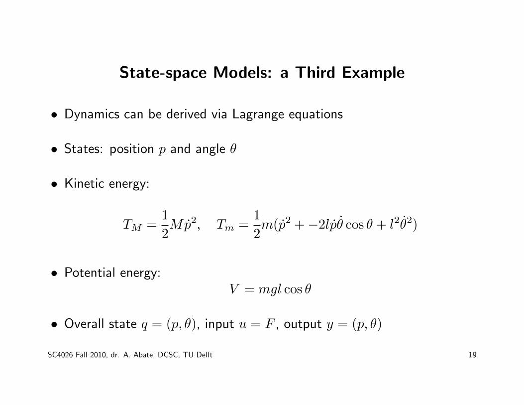
State-space Models: a Third Example
• Dynamics can be derived via Lagrange equations
• States: position p and angle θ
• Kinetic energy:
TM =1
2Mp2, Tm =
1
2m(p2 +−2lpθ cos θ + l2θ2)
• Potential energy:V = mgl cos θ
• Overall state q = (p, θ), input u = F , output y = (p, θ)
SC4026 Fall 2010, dr. A. Abate, DCSC, TU Delft 19
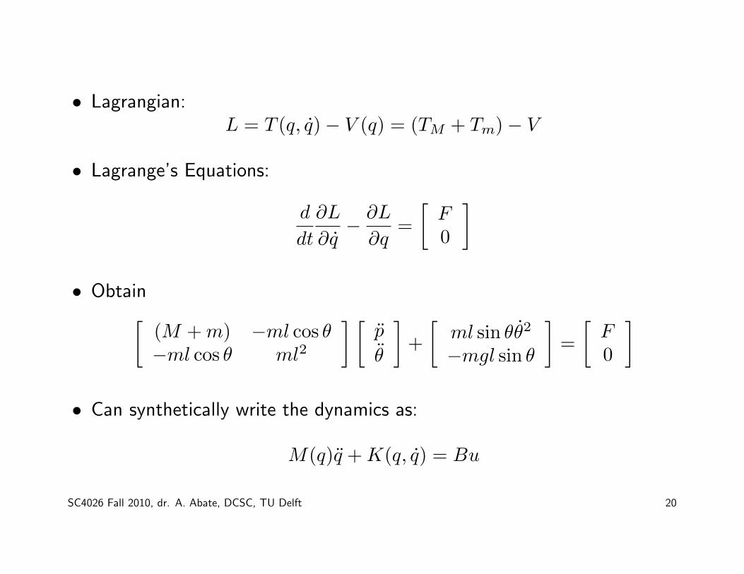
• Lagrangian:L = T (q, q)− V (q) = (TM + Tm)− V
• Lagrange’s Equations:
d
dt
∂L
∂q− ∂L
∂q=
[F0
]
• Obtain[(M +m) −ml cos θ−ml cos θ ml2
] [p
θ
]+
[ml sin θθ2
−mgl sin θ
]=
[F0
]
• Can synthetically write the dynamics as:
M(q)q +K(q, q) = Bu
SC4026 Fall 2010, dr. A. Abate, DCSC, TU Delft 20
• Notice that we have built a nonlinear model
• The model will be “linearized” in Lecture 2
SC4026 Fall 2010, dr. A. Abate, DCSC, TU Delft 21