Control system of person following robot:

The indoor exploration subtask

Solaiman. Shokur

20th February 2004

Contents

1 Introduction 31.1 An historical overview . . . . . . . . . . . . . . . . . . . . . . 31.2 Reactive, pro-active and Hybrid agents . . . . . . . . . . . . . 41.3 Problem Statement . . . . . . . . . . . . . . . . . . . . . . . . 51.4 Thesis outline . . . . . . . . . . . . . . . . . . . . . . . . . . . 5

2 Method 62.1 Evolutionary Robotics using simulator . . . . . . . . . . . . . 62.2 Realistic simulation . . . . . . . . . . . . . . . . . . . . . . . . 62.3 Calculating the relative position: Odometry and magnetic

compass . . . . . . . . . . . . . . . . . . . . . . . . . . . . . . 7

3 State of Art 93.1 Human Target following project . . . . . . . . . . . . . . . . . 93.2 Spatial information in Robots . . . . . . . . . . . . . . . . . . 103.3 Spatial information in animals . . . . . . . . . . . . . . . . . 113.4 Exploring an unknown environment . . . . . . . . . . . . . . 12

4 Exploration 144.1 Why is Exploration ability useful for this project . . . . . . . 144.2 Formalization of the Exploration task . . . . . . . . . . . . . 144.3 What is a complicated Environment? . . . . . . . . . . . . . . 15

4.3.1 Internal Rooms . . . . . . . . . . . . . . . . . . . . . . 154.3.2 Two types of aliasing problems . . . . . . . . . . . . . 18

5 Precedent work on this project 215.1 The transmitter-receiver Device . . . . . . . . . . . . . . . . . 215.2 Implementation of the human target following robot . . . . . 22

5.2.1 Experiments Setup . . . . . . . . . . . . . . . . . . . . 235.2.2 Results and Critics . . . . . . . . . . . . . . . . . . . . 24

6 Experiments 276.1 Experiments Setup . . . . . . . . . . . . . . . . . . . . . . . . 276.2 Simple reactive agents . . . . . . . . . . . . . . . . . . . . . . 29

1

6.3 Stochastic Neuron . . . . . . . . . . . . . . . . . . . . . . . . 316.4 External memory encoding the previous robot position . . . . 376.5 Modular architectures . . . . . . . . . . . . . . . . . . . . . . 41

6.5.1 Redefinition of exploration . . . . . . . . . . . . . . . 426.5.2 Evolving a good wall following strategy . . . . . . . . 446.5.3 Evolve two separated Neural Networks . . . . . . . . . 456.5.4 Define a sequence of Left and Right following . . . . . 476.5.5 Results and critics . . . . . . . . . . . . . . . . . . . . 50

7 Conclusion 53

A Graphs 59

B Demonstration 61

2

Chapter 1

Introduction

The goal of the main project is to develop a mobile robot able to find, fol-low, and monitor a human target moving in a domestic environment. Thisproject involves both hardware and software components and is part of theRoboCare Project 1. The hardware part includes a research for differenttypes of sensors able to locate a distant target, in particular the implemen-tation of a directional radio transmitter and receiver.On the other side, my scope was to manage the exploration task, that oc-curs when the robot looses the target. My research includes: definition ofthe fitness function, research for a convenient neural network architecture,definition of a strategy of evolution and definition of a realistic environmentfor the simulation.

1.1 An historical overview: Embodied CognitiveScience

The Embodied Cognitive Science represents a different and exciting newpoint of view challenging the traditional cognitivism and connessionism .The traditional cognitivism, born in the middle of the past century, was aresponse to the behaviorist point of view, which described all psychologi-cal states as sets of stimuli and the response of the body to those stimuli,defining the mechanism between them as a black box. The cognitivism givesan answer to these black boxes, saying that what is actually between thestimulus and the response is a computer (John Searle: ”The idea is that

1The goal of the RoboCare project is to build a multi-agent system which generatesuser services for human assistance. The system is to be implemented on a distributed andheterogeneous platform, consisting of a hardware and software prototype. The projectis funded by the Italian Ministry of Education, University and Research (MIUR). It isorganized in 3 tasks: 1. Development of a HW/SW framework to support the system2. Study and implementation of a supervisor agent 3. Realization of robotic agents andtechnology integration; for more information see http://pst.ip.rm.cnr.it/robocare/

3

unless you believe in the existence of immortal Cartesian souls, you mustbelieve that the brain is a computer” [4]).However according to our everyday life experience, great differences appearsbetween a human brain and a computer : if the brain is a computer, why isit, that what is easy for the brain is so difficult for a computer (recognition ofan object for example) and, in the opposite way, what is easy for a computeris so difficult for the brain (calculation) (ref. Parisi D., Oral communication).The classical connessionism gives another answer to the black box: a the-oretical neural network expressed as a computer programm. A progress inthis direction has been proposed by Embodied Cognitive Science consid-ering the agent (with a neural network) and the environment as a singlesystem, i.e. saying that the two aspects are so intimately connected that adescription of each of them in isolation does not make much sense [5, 10].This work uses these new research paradigms, that is Neural Networks,sensory-motor coordination, to satisfy a technological and theoretical prob-lem.

1.2 Reactive, pro-active and Hybrid agents

Typical reactive agents are the Braitenberg vehicles [11], which respond al-ways in the same way to the same sensory input. As we will see this kindof stereotypical behavior is often not satisfying for an exploration task.

On the other hand, recent work have shown interesting results, for tasks sim-ilar to our’s, with pro-active agents. Pro-active agents actions don’t dependonly on the sensory input but also on an ”internal state” that is defined asthe subset of variables that co-determine the future input-output mapping ofthe agent. Typically, an internal state is realized by a neural controller thattranslates present and past sensory inputs into actions. Miglino et all haveshown recently that introducing an internal state increases significantly per-formance of an agent that must make a detour around an obstacle to reacha target [17]. Nolfi S. and Guido de Croon demonstrated the importance ofinternal states for the self localization task [20, 21]. However, these worksshow also that introduction of internal states raises the level of complexity.Prediction and analysis are very difficult, understanding how internal statesare used by the agents is often all but obvious.Instead, we decided to work on a hybrid form of agent, adding both ad-vantages of the two precedent types: simplicity of analysis of the reactiveagent and variability of the behavior of the pro-active agents. We obtainthis compromise by implementing reactive agents controlled by: a neuralnetwork with a stochastic input, a neural network with an input using anexternal memory encoding the robot’s previous position and a modular neu-ral network.

4

1.3 Problem Statement

My main work was to solve the problem of finding the target when therobot was lost, i.e when there is no information from the distal sensors (forexample radio sensor). In this case the robot should be able to explore theenvironment until it has the information about the target again.Many research works for exploration task in robotic use a method calledInternal map. Basically, the robot evolves in an environment and registersits movements to obtain a map (see section 3.2). This kind of method arenot very robust and have many problems in a complex changing and realisticenvironment. My work was focused on another point of view:

Define a robust strategy, using evolutionary robotics methods, to performthe exploration task with (Hybrid) reactive agents. For this task we will havetwo constraints:

. Space: The robot should be able to explore every part of the environ-ment

. Time: It has to do it as fast as possible, avoiding as much as possiblecycles.

1.4 Thesis outline

The outline of the thesis is as follows: in chapter 2, we explain methodsused for this project as the sampling method and the evolutionary roboticsBasic theoretical knowledge as neural networks and genetic algorithms arenot presented here. Interested readers could read chapter 2 in ”Evolution-ary Robotics” written by Nolfi S. and Floreano D. [12] as an introduction tothese notions. Following a bio-inspired engineering point of view, we give inchapter 3 an overview of spatial information integration b both in roboticsand with animals. In addition another project working on the human targetfollowing is briefly presented. In chapter 4, we explain more precisely whatwe mean by exploration, presenting what makes it complicated. Chapter 5presents the departure point of my project, where we explain the precedentimplementations of the human target following, its results and its limita-tions, that we tried to overcome in my project. All my experiments andresults are explained in detail in chapter 6. Chapter 7 concludes the re-search, reassuming the most interesting results and the next possible stepsto ameliorate them.

5

Chapter 2

Method

2.1 Evolutionary Robotics using simulator

Evolutionary Robotics, based on the darwinian evolutionary process, permitto find robust robot controllers, difficult to find with handcraft implementa-tion. The process begins with creation of a set of random genotypes definingthe weights of the neural networks that control the robots. All these con-trollers are applied to a task and receive a score proportional to their abilityto perform it. At the end of a determinate life-time, we select those who havethe best score and use them for the next generation, after having appliedthe genetic operators (crossing over and mutation). The process continuestill having a controller that performs perfectly the task or until a stoppingcriterion is met.As an evolutionary process involving real Robots could be excessively expen-sive in term of time, a simulation approach using a realistic representationof the real robot and of the environment is preferred. The idea is first to leta good controller evolve in simulation and, in a second time, continue theevolution on the real Robot. The simulator used for this project is Evorobot[1] , that permits realistic experiments and the transition to real robots. Fol-lowing this reasoning, we implement a realistic representation of the robotKoala (that will be used as real robot for the project) on Evorobot.

2.2 Realistic simulation

As experiences on the simulator are a preliminary step before the use of areal robot, there is an obvious interest to make them as realistic as possible.The robot that will be used for the human target following task will be aKoala. The Koala has been preferred to the Khepera robot for practicalreasons, as the Koala has bigger dimensions and gives the possibility to usethe radio transmitter and receiver. The problem was that in the Evorobotsoftware only the Khepera robot was simulated. To be able to simulate the

6

Koala Robot, we have done some changes in the code:

- The dimensions of the simulated robot (30 x 30 cm for the Koala, 7cm diameter for the Khepera) have been changed

- The maximum speed (0.6 ms for the Koala and 1 m

s for the Khepera)has been modified.

- The sensors have been accurately changed as:

. The Koala has 16 infrared and ambient sensors, Khepera has 8

. The maximum range of this sensor is 20cm for the Koala and 5cmfor the Khepera

One way to simulate this sensors could be to implement their behavior byusing their theoretical specificities (i.e using the non-linear function of lightreflected value versus the distance to an obstacle). However, this methodappears dramatically irrelevant for simulating realistic cases.First of all, even if all the sensors of the Koala appear identical, they oftenresponse in a different way to the same external stimulus, given their intrinsicproperties. In addition, if one compares different robots, one notices thatthe position and the orientation of the sensors are not exactly the same.Finally, the Koala’s sensors are not distance measurements but a measureof the quantity of light that a given obstacle reflects back to the robot. Thusthis measure depends of the reflexivity of the obstacle (color, kind of surface,. . . ), the shape of the object, and the ambient light settingsA more interesting way to simulate these sensors according to their speci-ficities is to empirically sample the different classes of objects that appearin the environment [3].Using this method, we have sampled three classes of objects : a wall, asmall cylinder (diameter smaller than the robot’s dimensions: 20cm) and abig cylinder (diameter bigger than the robot’s dimensions: 42cm). The realrobot was first placed in front of one of these objects (distance 5cm), andthen automatically recorded all its sensors for 180 orientations and for 20different distances. In the simulator, given the orientation and the distanceof the simulated robot to a given obstacle, the corresponding line in thesampling file is used as input vector.

2.3 Calculating the relative position: Odometryand magnetic compass

The Koala has an internal counter that calculates exactly how much the mo-tors turn [2]. Using the right and left motor counters, one could determinethe position of the Koala at every time step. Unfortunately, even if the inter-nal counter for the motors is exactly known, the calculation for the position

7

of the Koala cannot be that precise, as the way in which Koala’s wheelsturn depends a lot on the kind of surface used. For example the Koala turnsmuch more easily on a smooth surface than on a carpet. We have estimatedan error rate of about 1% between the position internally calculated by theKoala (based on the motor’s counter), and it’s real position. Calculus wasdone as follows: the Koala randomly moves in the environment and registersits position, after approximately 10 meters covered, the robot is asked to goback to the initial position (set as (0.0) position). We calculated then thedifference between the effective initial point and this new point. For a morerealistic simulation, this error rate was introduced in the simulator whenodometry was used.Our test shows also that the error rate of the calculus made by the robotfor its position increases when the robot turns. In fact, tests with a Robotthat had to go only forward and come back to the initial point were muchmore precise (less then 0.5% of error). What increases the error rate is theaccumulation of errors on the angle. To avoid this we could add a magneticcompass to the Koala. This kind of component has been successfully usedby the K-team on the Koala (ref. Mondada F. Oral communication).In our case, as we didn’t test a magnetic component, we didn’t simulate iton Evorobot, we simply assume that having 1% of error on the position isnot unrealistic. A more precise and accurate estimation could be done whenthis this component will be available.

8

Chapter 3

State of Art

3.1 Human Target following project

Bahadori S. et all, also involved in the Robocare project, are developingrobots for the same task of ”human target following”, but with a very dif-ferent point of view [23]. Their work is mainly based on 3D reconstructionsthrough Stereo Vision. By computing a difference between a stored im-age, representing the background, and new images, they isolate the movingobjects (as robots and persons) from the environment. The robot is dif-ferentiated from persons with a particular marker. Then, by using stereocomputation, the position of the robot and the person are found.

The main idea for the next step is to use this information about robots’ andpersons’ position to manage the target following task, with some planifica-tion algorithms.The limitation of such a system are the following:

- The number of persons in the room has to be limited, the movingobjects could be of a maximum 3 or 4.

- The person should be easily differentiable from the robot.

- If one wants to cover a big room, or even maybe several rooms, thenumber of stereo cameras needed could become high.

I think that the third point here is very important, as, although, this ap-proach is highly interesting if one needs a Robot that has to follow the targetin a small area, it become really expensive because of the number of stereocameras involved and the complexity of installation (which is different forevery type of surroundings).

9

3.2 Spatial information in Robots

Robots that have to explore an environment is certainly one of the mostclassical problems in the filed of robotics . Implementation of robots ableto go out of a labyrinth is a typical exercise proposed to students 1 aswell as studied by researchers [26]. The most common way to manage theexploration with robots is to use internal maps. We will see here the twovery general ways of using internal maps: static and dynamic maps.The static map is certainly the easiest way to manage the exploration prob-lem, but could often be irrelevant. The main idea is to have a geometricrepresentation layer of a particular environment and topological layer. Forexample, the letters A to F in the geometrical map shown in figure 4.1 arethe identifiers of the topological regions which can be seen as nodes of anindirect graph (see appendix A). Using odometry and complex sensory in-puts2 the robot could be able to keep the track of its current position andorientation. Using a list of all unvisited rooms and the paths to join them(given by the topological graph), the robot is able to optimally explore theenvironment avoiding cycles. This method could be successfully used if onecould have a perfect a priori knowledge of the environment and also needsa robot able to explore a particular environment (as used, for example, byJohan Bos and all [27]) but cannot be applied if we want to have a generalexploration method for any kind of environment.

Instead, robots using a dynamic internal map do not need an a priori mapof the environment, the map is dynamically created by the robot duringexploration. Here, the topological layer is created step by step with roughly:recognition of the environment with sensory inputs and odometry. Therecognition of the environment implies huge and precise sensory informationto be used. The problem that particulary occurs for robots with poor sensoryinformation (as in our case), is that different places of the environmentcould give the same sensory vector input (known as the aliasing problem[13]), and so it is impossible for the robot to know if it has already been ina particular position or not. The limitation of odometry is that it is veryimprecise and sensitive to error cumulation, and the classical way to managethis accumulation is to re-initialize periodically the position at which therobot identifies perfectly a particular position where it has already been,what is limited again by the sensory information poorness. The typicalproblem that occurs in this kind of method is that one has to stress withtwo source of information, that may not concord. The robot, calculates it’sposition with odometry, and sensory inputs are used for the internal map.When robot wrongly think to be in a point where it has already been, and

1http://diwww.epfl.ch/ sshokur/projets/matinfo.zip2Often for this kind of method video cameras are used

10

the sensory input do not coincide with the registered input, it has to re-actualize, or its position (what it think to be it’s position) or the internalmap. Actually, it’s very difficult to decide which one of the two informationhave to be actualized, as both odometry and environment recognition couldbe erroneous.

3.3 Spatial information in animals

There are two principal points of view about animals’ strategy to managewith the surrounding environment. The main difference between them isabout the referential that animals use to integrate information about theenvironment: egocentric or exocentric coding.In a behaviorist point of view, exploration of an animal could be traduced asa simple association between stimulus and responses. For example, the wayto go from one initial point to a food zone will be registered by the animalas a series of movement that will be reproduced if we put the animal againin the initial position [6]. The method could be used by the animals even forlong and difficult ways by dividing the road in different little subsequences.In this case the information about the environment is coded according tothe animal itself : the referential is egocentric. Another use of egocentricreferential has been shown by Wehner et al. for the homing navigation of thedesert ants Cataglyphis, who can explore a long distance and return directlyto the nest. They explain that this ants register all their movements duringthe exploration for food and that they integrate them to derive the directionto go back to the nest.The advantage of of egocentric reference coding is to limit the informationto be registered to only two parameters: angle and distance. However, it isvery difficult to know exactly these two parameters as they are extremelysensitive to error cumulation, especially for the angle [8]. To avoid thisaccumulation different techniques are used by animals: birds for exampleuse magnetic compass for calculating angle during their long migrations.Insects, in particular ants and bees, use sunlight compass derived by theazimuthal position as well as from spectral gradient in the sky. Hartmannand Wehner have shown how path integration based on solar compass isimplemented neurophysiologically to perform homing navigation [28]. Ratsre-initialize their information when they recognize a particular place thatthey had already visited [18, 19].This very easy and rapid strategy is certainly used by animals for somechanges of location, but could be irrelevant in a changing environment. Forexample, if the position of an object is changed or if an object is added, thismethod could fail.

The second point of view has been proposed by O’Keefe and Nadel in 1978

11

[14], and is the base of what is called a ”cognitive carte”. For animals,as well as for humans beings, the part of the brain that manage the spaceapprehension and representation is the hippocampus, with the location cel-lular as neural support. In the case of rats for example location cellular,are activated when they are in a particular position of the environment.The importance of location cellular has been demonstrated in an experi-ment involving rats: those who had lesion in the hippocampus were unableto manage with exploration subtasks such as distinguishing visited and nonvisited ways in a labyrinth [9].

In this case information about the environment is registered referred to fixedreference marks extracted from the surroundings. The animal registers thereciprocal relation between different places. This method is efficient evenif some parts of the environment change and in the worst case, as it hasbeen shown for the rats, if the environment changes too much, there is aselective re-exploration. However, it is not yet very clear what are the fixedreferences to be registered and how these are integrated by animals.

3.4 Exploring an unknown environment

We will discuss here the techniques used in robotics or inspired by naturethat could be useful for us. Remember that our task is to accurately exploreany environment, avoiding as much as possible cycles.We have seen classical solutions used in robotics: use of a static or a dynamicinternal map. The first technique has to be immediately rejected, as it isnot a general way to explore any environment.We have to be careful not to confuse dynamical internal maps in roboticsand cognitive maps in animals, as internal maps could be performed withegocentric or exocentric information (contrary of animals where the notionof cognitive map is associated only with exocentric coding3). An exocentricregistration of the surroundings implies the recognition of particular placesin the environment and the relations between them. This method requiresa huge amount of information about the environment [31]. For example forrats, which recognize some parts of the environment (proved by the factthat there are specific location cells that are activated only when the Ratis in a particular place [14]) there are a lot of different sensorial modalitiesused : visual seems to be the most important, but audition and smell arealso involved (as shown by Hill and Best, even blind rats use location cel-lular [22]). So there is a huge amount of information (think about visionthat involves color, distance, shapes, . . . ) used to detect unambiguously aparticular position of the space. Compared to the rat, our sensory infor-mation (16 Infra-red proximity and ambient light sensors) is dramatically

3if we accept the definition given by O’Keefe and Nadel [14]

12

poor. Robotic projects using these kind of techniques are confronted to adilemma: augmenting the sensory information by adding video cameras andtechniques of image analyze that slow down the robots’ behavior (see 3.1),or limit the exploration task to very simple environments (see [26]). Wewould like to avoid both disadvantages.

In the other hand we have seen that the problem of egocentric informationis the possible cumulation of errors, that could be corrected with externalreference: for example sunlight for insects, environment recognition for Ratsor magnetic compass for birds.A solution inspired by insects has been successfully implemented by Kim D.and Hallam J. C. T. [30] on a simulated Khepera. They have shown howa robot can use a referential light source, as a lamp, to perform homingnavigation. However, as in our case the robot has to explore more than onesingle room, this technique cannot work.The problem of landmark recognition is the same as in the exocentric coding:it implies more sensory input information to avoid aliasing problems.Instead, a method inspired by birds using a magnetic compass could be moreinteresting, we could use it compounded with odometry to avoid angle errorcumulation and having an egocentric information about the environment.Thus we decided not to use internal - dynamic or static - maps. We tried tofind other kinds of techniques using egocentric information, in a more easyand less dependant on error way (see in section 6.4) or even technics notusing at all egocentric information (see section 6.3 and 6.5).

13

Chapter 4

Exploration

4.1 Why is Exploration ability useful for this project

The ability to correctly explore an environment is very useful for a robotwhich has to follow a human target. We propose here two situations wherethis ability occurs:

- When the robot looses the target, i.e when it has no information fromthe distal sensors (example radio sensor) because of the distance.

- When there is an obstacle between the robot and the target that hasto be circumvented (losing may be temporarily the information fromthe distal sensor)

In these two cases, the robot has to explore the environment till it has againinformation about the target.

4.2 Formalization of the Exploration task

In our study, we will split the problems in two sub-problems: followingthe target and exploring. By exploration, we mean that the robot shouldbe able to visit any part, or any rooms, of any realistic environment. Wecan formalize the problem as a problem of research on an undirect GraphG(V, E,Ψ) (see Appendix A), where V (node) is the set of all rooms of theenvironment, E the set of all doors (see figure 4.1), and Ψ the function thatassociates for each door the two rooms separated by the corresponding door.

Thus our problem could be formalized as Graph Searching with visit of allnodes and the avoidance of cycles as constraints.

Notice that the set of environments EV that we will consider, are thosewho’s corresponding graph G(V, E,Ψ) is connected. That means that the

14

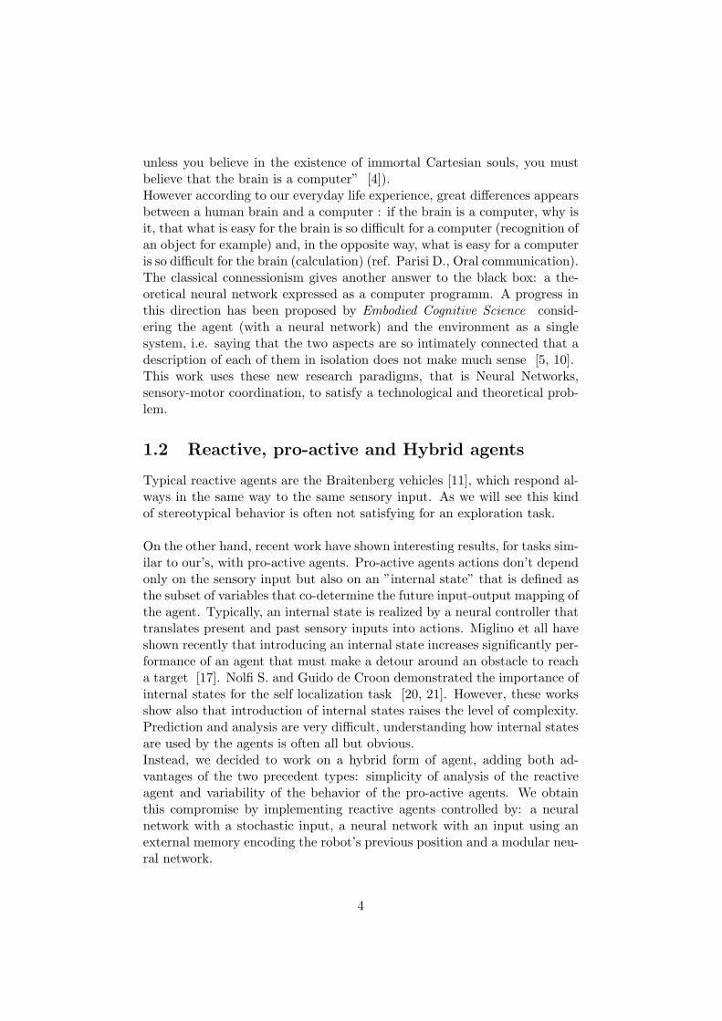
Figure 4.1: (Right) Environment E0 defined with rooms A,B,C,D,E,F; (Left)Graph G(V, E,Ψ) of E0: where V = {A,B, C,D, E, F} the set of rooms inE0 and E = the set of doors

excluded environments, are those, very degenerated, that have rooms thatcannot be joined by the other rooms (example rooms without door).We will define a strategy as acceptable if one who follows it is able to visitat least one time every room and we will say that a strategy is optimal ifit permits to visit all rooms avoiding any cycle.

So we have basically two different sorts of constraints: space (the explo-ration strategy should permit to go in every room) and time (it should doit as fast as possible). In our case, it is highly unrealistic to look for anoptimal solution. Instead, we will say that a strategy is satisfying, evenif it is suboptimal, if it is acceptable and avoids as much as possible cycles.

4.3 What is a complicated Environment?

One of the most challenging problem was to define a good environment,representative of realistic complications that occur in real environments,what is quite different from what appears intuitively complicated.

4.3.1 Internal Rooms

Let us consider a labyrinth1 that could appear as being complicated (figure4.2).

1from http://www.BillsGames.com/mazegenerator

15

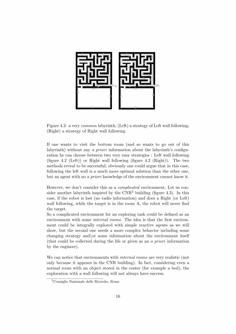
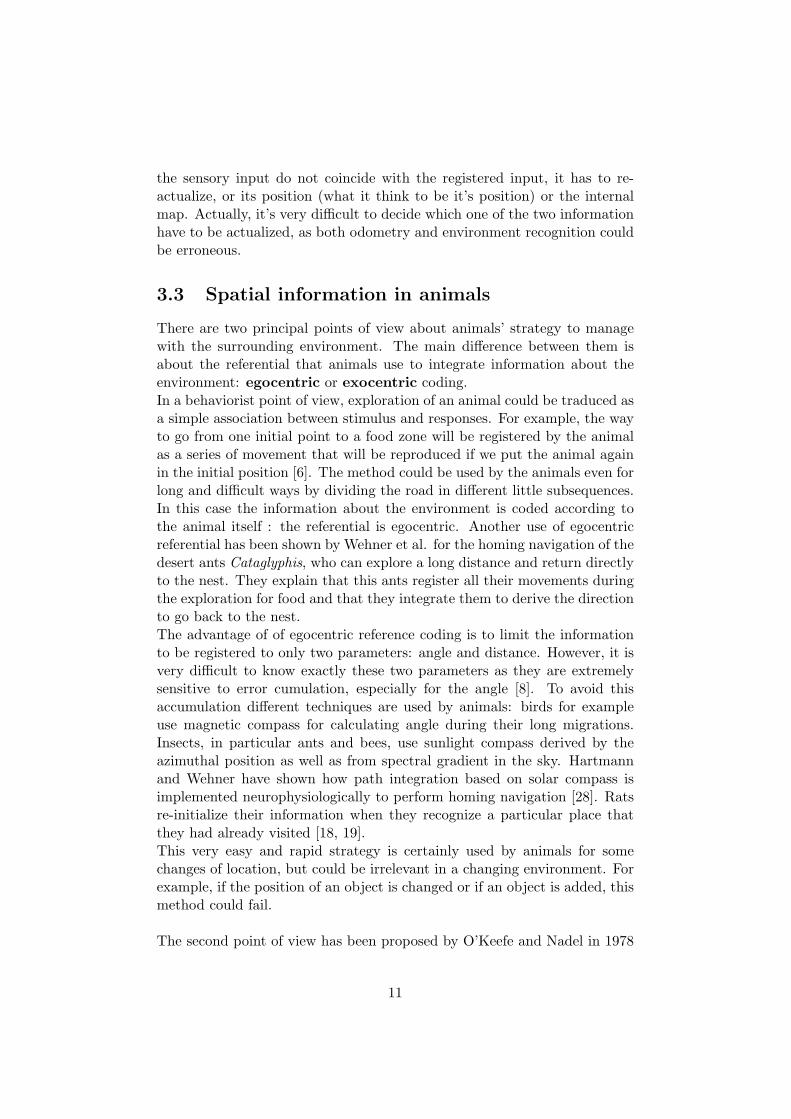
Figure 4.2: a very common labyrinth, (Left) a strategy of Left wall following;(Right) a strategy of Right wall following

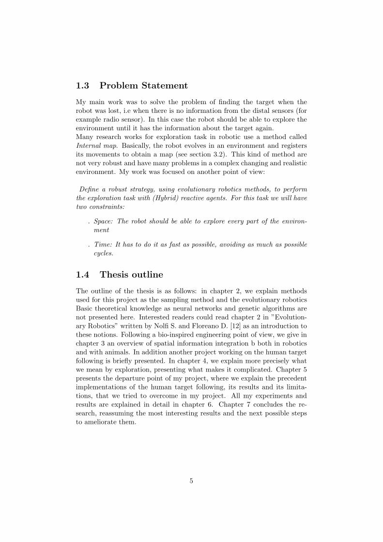
If one wants to visit the bottom room (and so wants to go out of thislabyrinth) without any a priori information about the labyrinth’s configu-ration he can choose between two very easy strategies : Left wall following(figure 4.2 (Left)) or Right wall following (figure 4.2 (Right)). The twomethods reveal to be successful; obviously one could argue that in this case,following the left wall is a much more optimal solution than the other one,but an agent with no a priori knowledge of the environment cannot know it.

However, we don’t consider this as a complicated environment. Let us con-sider another labyrinth inspired by the CNR2 building (figure 4.3). In thiscase, if the robot is lost (no radio information) and does a Right (or Left)wall following, while the target is in the room A, the robot will never findthe target.So a complicated environment for an exploring task could be defined as anenvironment with some internal rooms. The idea is that the first environ-ment could be integrally explored with simple reactive agents as we willshow, but the second one needs a more complex behavior including somechanging strategy and\or some information about the environment itself(that could be collected during the life or given as an a priori informationby the engineer).

We can notice that environments with internal rooms are very realistic (notonly because it appears in the CNR building). In fact, considering even anormal room with an object stored in the center (for example a bed), theexploration with a wall following will not always have success.

2Consiglio Nazionale delle Ricerche, Rome

16

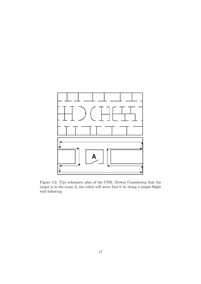
Figure 4.3: [Up] schematic plan of the CNR; [Down] Considering that thetarget is in the room A, the robot will never find it by doing a simple Rightwall following

17

Figure 4.4: Aliasing problem during exploration: when the robot is in theshaded part of the corridor it has to go one time straight on(A)and the othertime to the left (B).

4.3.2 Two types of aliasing problems

A second source of complication for exploring an environment is the aliasingproblem [13]. An aliasing problem occurs in our case if we have one singleplace with at least two different possible ways or if there are two (or more)different places that give the same input vector but need different responses(example one time going right, another time going left ).An example for the first aliasing problem could be a normal corridor. Aswe could see on figure 4.4, when the robot is in the middle of the corridor(shaded), it has two different possible choices. To be able to explore all theenvironment, it should certainly go at least one time in each direction (Aand B). We could notice that this aliasing problem occurs if and only if wehave an internal room as shown in figure 4.5.The second aliasing problem is also particulary present in our case becauseof the dramatically poor sensory information. As said we have omly 16infrared ambient sensors.These two types of aliasing problems complicate the exploration task asfollows:

- The first type of aliasing renders the exploration task complicated interms of space. We will show that a simple reactive agent is not ableto visit an environment integrally if the first aliasing problem occurs.

- The second type of aliasing renders the exploration task complicatedin terms of time. In an environment without any second type aliasing,an agent can be evolved to recognize exactly if it has already been in aparticular point of the environment and could easily avoid cycles (byfor example changing its direction or strategy of exploration).

In other words, an easy environment can be entirely explored by a simplereactive agent (which always responds in the same way to the same sensory

18

Figure 4.5: (Left) if there is no internal room, by using a simple wall fol-lowing a robot could explore both direction in a corridor (Right) The robotcannot visit both direction with a wall following, the robot should have twodifferent behaviors for the same sensor information

inputs). As defined above, an internal room gives another level of complexitythat prevents simple reactive agents to solve the exploration task.However, we will see that there are different ways to define an environmentwith an internal room that gives also a different level of complexity (seesection 6.3).As we will see, another important parameter for the complexity of an en-vironment is the size. The main problem with a big size environment isto manage the cycles, because there is a direct correlation between the sizeof cycles and the size of memory required. It is intuitively obvious that ifone wants to perceive a cycle, one should be able to detect some kind ofperiodicity, and the more the period is long, the more memory is used todetect it.

19

Figure 4.6: Three environments used for our experiments, the littleround in the corners are artificially added to give thickness to thewalls;(Left)Environment 1; (Middle)Environment 2; (Right)Environment 3

20

Chapter 5

Precedent work on thisproject

Before my project, some tests were done for this specific task. We willsee in this chapter the results and some limitations that appear in thoseexperiments.

5.1 The transmitter-receiver Device

To allow a robot to localize a distant target, even separated by an obstacle, aradio type transmitter-receiver system consisting of a transmitter carried bythe target person and a receiver installed on the robot is under developmentat the CNR by Raffaele Bianco, Massimiliano Caretti and Stefano Nolfi[16]. This new sensor will permit the robot to find the relative direction ofthe human target. Preliminary tests of this system indicate that it providesreliable information about direction but not about the distance of the target.The system consists of a transmitter producing a continuous signal of 433MHz (figure 5.1 Left), a receiver (figure 5.1 Top-Right), and a directional an-tenna (figure 5.1 Bottom-Right). To provide information about the currentdirection of the transmitter the antenna should be mounted on a motorizedsupport (still to be developed) that allows the rotation of the antenna andthe detection of its current orientation with respect to the frontal directionof the robot.A second more precise sensor that could give additional information aboutthe distance of the target is also under development at the CNR. The mainidea is the same as for the first one but it uses sound instead of radio waves.The system consists of a transmitter (on the target) producing very shortsounds separated in time and a receiver (on the robot) provided with twoomni-directional microphones that detects the arrival of the first waves andthen stop listening until echoes have disappeared. The receiver device detectthe time difference between the signals detected by the two microphones that

21

Figure 5.1: The radio transmitter-receiver device. Left: The transmitter.Top-Right: The receiver. Bottom-Right: The antenna.

provides information about both direction and distance.

5.2 Implementation of the human target followingrobot

The human target following robot was already implemented in the simulatorEvorobot by Raffaele Bianco at the CNR (see figure 5.2). Here are the newcomponents added by him into the Evorobot simulator:

- A moving target has been implemented. This agent moves freely inthe environment. It avoids obviously the obstacles and at each stephe randomly it choses between turning right or left, going straight,accelerating, decelerating or even not moving at all.

- A directional sensor (see section 5.1) has been implemented. Thiscomponent is a very simplified implementation of the radio transmitterand receiver. As the knowledge about the real radio transmitter and

22

Figure 5.2: Koala Robot and the directional radio transmitter/receiver sim-ulated on Evorobot, the receiver divides the environment in three zone cor-responding to three input of the robot, if the target is in one of these zones(no matter its’ distance) the corresponding input is activated

receiver component is low, the simulator includes simply three inputsthat divide the space in front of the robot, and which are activated ifthe target is in the corresponding section (see figure 5.2).

One could argue that this simulation is not realistic at all as it doesn’tmanage any distance problems, in particular there is no attenuation of in-formation if there is an obstacle between the robot and the target or if thetarget is very far. In addition, in the real case, we could have some interfer-ence problems with the radio waves in a room, or attenuation of the signalif there is an open window or a closed door,. . . All this data will be knownonly when the radio sensor will be completely implemented, tested and sam-pled to be used by the simulator. Therefore we decided to concentrate ourwork on more theoretical problems, that are useful for the next step of theproject.In fact, even if we don’t know exactly how the sensor reacts, there is at leastone certainty: in some cases the robot will be lost. For example if the targetis too far or if there is an obstacle between the robot and the target. Wedon’t have to know if too far means exactly 20.5 or 30.4 meters. In this casethe robot should be able to explore the environment to find the target (orfor having some radio information again).

5.2.1 Experiments Setup

We will see in this section how the first experiments done by Raffaele Biancowere implemented.The fitness function defined for this first experiment was:

1/distance between the robot and the target (5.1)

This function has some limitations:

- As it is not possible to know what is the maximum value: interpreta-tion in term of optimal performance is not possible.

23

Figure 5.3: Evolved agent following the target, Simulated Koala Robot withthe directional radio sensor, The evolved agent tries to minimize his distancewith the target

- It is an external function : the variable distance between the robotand the target is not available to the robot it self, and could requirecomplex machineries and procedures if we project to evolve a real robot(p.64-66 in [12]).

- The evolved individuals are not able to follow the target in all casesas we will see in the next section.

The architecture of neural network was a standard feedforward , with 11input i.e. 8 infra-red proximity sensors of the Khepera (the Koala’s sensorsweren’t yet sampled) plus 3 inputs of the radio type sensors and 2 outputfor Khepera’s motor left and right controllers. The environment was the oneshown in figure 5.4.

5.2.2 Results and Critics

In the very first part of the project I have tried to identify situations thatevolved agents, found with this first implementation, did’n’t manage.

The best individuals of these first experiments show a very good ability tofollow the target in an easy environment, defined as a box with no obstacle(see figure 5.3).Using a more complicated environment with obstacles, the agent shows stillgood abilities to follow the target. In fact in some of these evolved agentsthere is emergence of wall following strategy when there is an obstacle be-tween them and the target.

24

Figure 5.4: Evolved agent following the target, with wall following strategywhen there is an obstacle

As shown in figure 5.4 this simple implementation gives a very good result.The main idea is that till the directional radio receiver has information (thedirectional receiver oriented in the direction of the transmitter), the robottries to minimize the distance with the transmitter (target), but when thisinformation is lost, it changes its strategy and begins a wall following. How-ever, the fact that sometimes the robot looses the radio information dependson the target movement. For example: the robot is against the wall, it triesto go in the target’s direction but an obstacle prevents it. Then, the targetmoves away and robot’s receiver loses the radio information, the robot stopstrying to go in a particular direction and follows the obstacle until it hasagain some radio information available. We could see on figure 5.5 whathappens if the target does not move and the radio information remains al-ways available to the robot. In those cases the agent does not go into a wallfollowing strategy and continues indefinitely with the first strategy (mini-mizing the distance).

However the problem of the blocked robot when the target is not moving isactually not a very serious one as we could resolve it by adding some randommovement to the blocked robot (it this case the robot will lose the directionof radio signal and begins a normal wall following).A much more serious problem is to define a good exploration strategy thatcould be used by the robot when it looses completely the radio signal andthe human target. We have seen that the only strategy used by the agentto explore the ambient, when looking for the target, is a wall following, thatis not enough for an acceptable exploration of any realistic environment (seesection 4) .

25

Figure 5.5: If the target (up Left) does not move and if there is an obstaclebetween the robot and the target, the robot is blocked indefinitely againstthe wall

26

Chapter 6

Experiments

In this section I will explain the experiences I have done to find agents ableto explore any realistic environment. The strategy was to evolve this agentsand to test them on some very general and some complicated environments.The definition of what is general and complicated was a difficult task. Infact I had to define environments for the testing part, that ensure us thatif the evolved agent was able to explore the totality of them, this agent willbe able theoretically to explore any environment. The environments usedare those defined in section 4 (Environment 1,2 and 3).

6.1 Experiments Setup

As the implementation of the simulation for the Koala was done during thelast part of my project (the real Koala Robot was available only the lastmonth), a huge part of the experiments has been done with the simulatedKhepera. Then when the Koala was correctly implemented some of themost interesting experiments were reproduced. Obviously, when we comparedifferent types of agents between them and give statistics of success rate, weuse only one type of simulated Robot.Evolution and tests for the next sections was done as follows: Agents wereevolved on Environment 1 (see figure 4.6), each experiment was reproducedat least 10 times. A population was composed of 100 randomly generatedindividuals, and was evolved for at least 300 generation. Individuals’ lifelasted 5 epochs of 5000 life steps. At the beginning of each epoch, theindividual was positioned randomly in the environment.The mutation ratewas 4%.Then the best individual of the best seed was tested 20 times on Environ-ments 1, 2 and 3. At the beginning of each epoch the start position wasrandomly selected. The life for the test was 20’000 time step, consideringthat an agent with an optimal strategy should be able to visit the environ-ment integrally in approximatively 4’000 time steps.

27

Fitness Function

The fitness function was defined as follows:

Fitness = φ + ψ (6.1)

Where φ is the obstacle avoidance function as defined by Floreano D. andMondada F. [15]:

φ = (V )(1−√

∆V )(1− i); 0 ≤ V ≤ 1; 0 ≤ ∆V ≤ 1; 0 ≤ i ≤ 1; (6.2)

With V: the sum of rotation speeds of the two wheels, v: the absolutevalue of the algebraic difference between the signed speed values of thewheels (positive is one direction, negative the other), and i: the normalizedactivation value of the infrared sensor with the highest activity.

And ψ defined by:

ψ =

positivescore, if the agent cross a door for the first time;0, every par time that the agent crosses the same door;negativescore, every odd time that the agent crosses the same door

and if | (fitness− negativescore) |≥ 0.(6.3)

The point was to force an individual to go into all rooms (+ score to crossa door) but to avoid to return into the same rooms. As par times are thosewhere the agents simply get out of a visited room, no positif or negativescore was given1. Obviously, if all rooms were visited the list of the visitedrooms was re-initialized (the agent could go back into a room that wasalready visited and have a positive score).

Many values of the positive and negative score have been tested. The mostinteresting solutions were obtained with a half incremental score:

- positive score = 5′000× number of visited rooms (+5000 for the firstcrossed door, + 10’000 for the second one, . . . )

- negative score = −5′0001Example: a agent crosses a door and goes into a room ⇒ positive score, it recrosses

the same door to get out of the room ⇒ no positive or negative score, it recrosses againthe same door ⇒ negative score, etc

28

The reason of an incremental positive score and a normal negative one, wasthat we prefered an agent a which visits three rooms and returns back intwo of them: fitness(a) =

∑3i=1 i ∗ 5′000 − (2 ∗ 5′000) = 20′000, to an

agent b which visits only two rooms fitness(b) =∑2

i=1 i ∗ 5′000 = 15′000,because agent a explores more space than agent b. Instead a normal positiveand negative score would give best fitness for agent b than for agent a:fitness(a) = 3∗5′000−(2∗5′000) < 2∗5′000 = fitness(b) and an incrementalpositive and negative would give the same fitness for both:

∑3i=1 i ∗ 5′000−∑2

i=1 i ∗ 5′000 =∑2

i=1 i ∗ 5′000 = 15′000.

6.2 Simple reactive agents

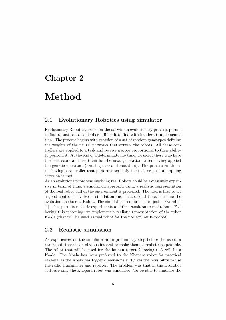
For these experiments, I have used some parts of the implementation doneby Raffaele Bianco (see 5.2) without using the simulated radio sensor.The first architecture tested was a simple feedforward with 16 input neurons(Koala’s sensors), 4 hidden neurons and 2 output neuron (Koala’s motor leftand right controllers).As previewed these simple reactive agents were only able at most to performa wall following and they never explored integrally an environment withinternal rooms (figure 6.1 (Right)). In addition, another problem thatoccurred here was that sometimes the agent could be blocked in a smallercycle (figure 6.1 (Left).In the next tabular the percent of complete exploration, of crash and partialexploration is reported. A partial exploration appears when the agent iseither or in micro cycles (in this case it visits often only one room) or inmacro cycles. The results are based on 20 tests for each Environments.

Environment1 Environment2 Environment3completely visited 0 0 0

crash 0 0 0partially visited 100 100 100

Change the obstacle avoidance fitness

We have defined our fitness function using the obstacle avoidance fitnessΦ (see equation 6.1), which gives a good score for individuals that havetendency to go straight (parameter ∆V ). In our case it could be desirableto have an agent that turns more, and that instead of going straight intointo corridors has the tendency to turn and enter in the different rooms. Sowe have changed the fitness function to give less importance to ∆V compareto the parameter speed V and the distance to the walls i:

φ′ = (V )(1− ϕ(∆V, k))(1− i) (6.4)

29

Figure 6.1: Typical behavior of a reactive agent: (Left) Micro-cycle(Right)Wall following and macro-cycles

With V , ∆V and i defined as in the normal obstacle avoidance fitness φ andϕ(x, k) = x+(k−1)

k .Test with three different values of k: 5,10 and 15 have been done. Onceagain the architecture was a simple feedforward neural network with 16input neurons (Koala’s sensors), 4 hidden neurons and 2 output neuron.Here are the results in function of the value of k (k=0 is the same agent asthe one presented in chapter 6.2).The percent of tests in which the agent has respectively explored all the en-vironment, crashed or explored only one part of the environment is reportedin the next table. The results are based on 20 tests for each value of k andeach Environments, the value is the average result for Environment 1, 2 and3.

k = 0 k = 5 k = 10 k = 15completely visited 0 6 4 0

crash 0 0 0 5partially visited 100 94 96 95

We could understand these results by comparing the path of the best indi-viduals of the best seed for each experiment. The main difference is aboutthe angle between the initial direction and final direction when the agentavoids a wall. The more k is high the more this angle is near of 180◦, as wecould see on figure 6.2. This ability to change direction could be more orless benefic. In fact, as we have seen results shows that for k = 5 the rate ofcomplete exploration raise. The main reason is that, instead of doing a wallfollowing (see k = 0) the new agent changes it’s direction and can sometimesenter in the internal room, as suggested in the figure. In the other hand what

30

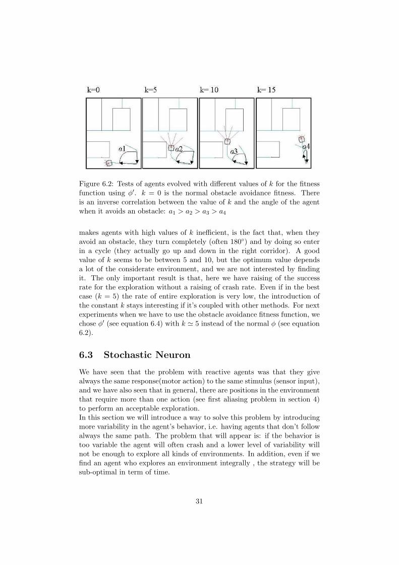
Figure 6.2: Tests of agents evolved with different values of k for the fitnessfunction using φ′. k = 0 is the normal obstacle avoidance fitness. Thereis an inverse correlation between the value of k and the angle of the agentwhen it avoids an obstacle: a1 > a2 > a3 > a4

makes agents with high values of k inefficient, is the fact that, when theyavoid an obstacle, they turn completely (often 180◦) and by doing so enterin a cycle (they actually go up and down in the right corridor). A goodvalue of k seems to be between 5 and 10, but the optimum value dependsa lot of the considerate environment, and we are not interested by findingit. The only important result is that, here we have raising of the successrate for the exploration without a raising of crash rate. Even if in the bestcase (k = 5) the rate of entire exploration is very low, the introduction ofthe constant k stays interesting if it’s coupled with other methods. For nextexperiments when we have to use the obstacle avoidance fitness function, wechose φ′ (see equation 6.4) with k ' 5 instead of the normal φ (see equation6.2).

6.3 Stochastic Neuron

We have seen that the problem with reactive agents was that they givealways the same response(motor action) to the same stimulus (sensor input),and we have also seen that in general, there are positions in the environmentthat require more than one action (see first aliasing problem in section 4)to perform an acceptable exploration.In this section we will introduce a way to solve this problem by introducingmore variability in the agent’s behavior, i.e. having agents that don’t followalways the same path. The problem that will appear is: if the behavior istoo variable the agent will often crash and a lower level of variability willnot be enough to explore all kinds of environments. In addition, even if wefind an agent who explores an environment integrally , the strategy will besub-optimal in term of time.

31

Figure 6.3: A fully connected neural network with a stochastic neuron;Input: 16 normalized infrared sensor of the Koala plus one stochastic neuron;4 hidden neurons; Output: 2 neurons that control the left and right motorcontrollers

”A man of genius does’t make mistakes,his mistakes are deliberate and are

gates of discovery”Philippe Sollers2

The idea, to develop an agent who has a more variable behavior was tointroduce a stochastic neuron. The architecture was as shown in figure 6.3:we had the 16 infrared sensors of the Koala as input, and in addition wehad one stochastic neuron with random values. We have implemented thestochastic neuron as follows:

Stochastic neuron[t] = k∗random value[t]+(1−k)∗random value[t-1]; 0 ≤ k ≤ 1(6.5)

The parameter k, gives somehow the level of randomness of the stochasticneuron, a value near to 1 gives a very variable neuron (and as we will see alsoa very variable behavior); contrary k near to 0 gives a neuron with valuesaround 0.5 and few variability and k = 0 gives a normal reactive agent asthose seen in section 6.2.The statistics of the experiments with different values of k (k = 1.0, 0.75, 0.5, 0.25, 0.0)and different sort of environment (Environment 1,2 and 3) are reported onfigure 6.4.

2Gisele Freud, Philippe Sollers, Trois jours avec James Joyce, 1982 Denoel, Paris

32

Figure 6.4: Agents with a stochastic neuron, tested on Environments 1,2and 3; X axis: value of the constant k (k = 0 corresponds to the reactiveagent) Y axis: type of exploration, Z axis: percentage of experiment (inbasis to 20 test for each type of experiment)

An accurate analysis of the statistics reveals that:

- The best agents are able, at most, to visit an environment integrally,in a third of case.

- The rate of acceptable tests and the rate of crash is correlated (corre-lation for the three environment = 0.59). That means that if we lookfor agents able to visit all the rooms by adding some kind of variabilityon its behavior, we augment its probability to crash

- A ”good” value of k depends of the environment. For example k = 0.75gives the best results for the first environment (33% of case it visitsthe environment integrally) but reveals to be inefficient in the thirdenvironment (100% of case it visits only 3

4 of the environment).

- The rate of crash and the rate of partial exploration is negativelycorrelated (correlation for the three environment = −0.91). Thosewho partially visit the environment are those who, by doing a wallfollowing, miss the internal room. Thus it seems that if one followswalls it’ is easier for it to avoid to crash.

First we will try to understand how the stochastic neuron with differentvalues of k is used by the agents.

33

Figure 6.5: The 5 agents with values of k = 0, 0.25, 0.5, 0.75 and 1.0, theagent are tested for 5000 life steps on an ambient where walls are not visiblefrom the starting point; (Up Right Squares) the variation of the center ofthe circular path that the agent is doing

The stochastic neuron gives some kind of noisy behavior to the agent (ascould be seen of figure 6.6 Right), but its contribution becomes really im-portant when the value of the infrared sensors are low, i.e when the agent isnot near a wall and has few information coming from the environment. Toillustrate this fact we test the five different agents in an ambient where thewalls are not visible (see figure 6.5).It is interesting to see that the space covered by the agents (in 5000 timesteps) is proportional to their value of k. The simple reactive agent, turnsalways in exactly the same way, when the other agents have tendency tochange the path. Notice that what we mean by ”covered space” has nothingto do with the diameter of the circle, but with the variation of the center ofthis circle, as shown into the right up squares.

Now we can try to explain the difference of success rate in function of envi-ronment and the value of k by analyzing an example of test with k = 0.75.We will also explain why this agent shows good abilities to explore Environ-ment 1, but not Environment 3.Let consider the best individual of the experiment with k = 0.75 and asimple reactive agent on Environment 1. When the simple reactive agent isin a macro-cycle, it always follows exactly the same path, whereas a reactive

34

robot with a stochastic neuron has a more changing path even when it is ina cycle as shown in figure 6.6(Left).If we compare the paths of the two different agents (figure 6.6(Right)), wecould notice several differences. The most interesting is the third one (figure6.6 (Right bottom)), that shows how the agent with stochastic neuron is ableto visit once the left room and another time the right room.The difference is about how the agent enters in the critical zone where it hasthe choice between more then one way. In Environment 1, in this particularposition, the values of the other sensor inputs are near to 0, as there is novisible wall on right or left. The simple reactive agent turns always withthe same angle (as we have seen on figure 6.5), even if we let the reactiveagent live a long time(example 20’000 life step when it does a cycle in 4’000life steps), nothing changes, it visits only three rooms, by doing exactly thesame cycles. Instead the agent with the stochastic neuron, when confrontedwith the critical zone, has variable behavior, the angle of turning could bedifferent from one to another passage.Now that we have explained why the agent with stochastic neuron has ahigher success rate than the normal reactive agent, we have to understandwhy its success rate is low when tested on Environment 3 (see figure 6.7)The problem here is that when the agent is in the critical zone (bottomright) the values of the other inputs are not low, so the stochastic neuroncannot be used to visit both directions.Notice also that in the corridors the agent’s path is not perfectly rectilinear,because of the noisy behavior introduced by the stochastic neuron. Thisfact explains also why the agent with k = 1, is sometimes able to exploreEnvironment 3. This agent has an even more noisy path into the corridors,and so, sometimes, when it arrives in the critical zone, it is far enough fromthe right wall to use the stochastic neuron and enter in the internal room.On the other hand, it is because of its very noisy behavior that its crashrate is so high.

This analysis could appear tiresome and very specific for one particular prob-lem to the reader, but actually it’s important to understand that introducingvariability we are in confronted to a dilemma, if the neuron is completelyrandom we have agent able to visit at least one time integrally any one ofthe three environment , but at same time we see the probability of crashingarise.Instead a stochastic neuron with a lower level of random (example k =0.75, 0.5) is useful for exploring a particular kind of environment: those inwhich the stochastic neurons which could be used in the critical zones. Inboth cases, it is not a satisfying strategy.

35

Figure 6.6: (Left) Path of a reactive agent with a stochastic neuron; (Right)Comparison between a simple reactive agent and a reactive agent with astochastic neuron; bottom how the second model of agent manages to explorethe internal room

Figure 6.7: Path of a reactive agent with a stochastic neuron (k=0.75),tested on Environment 3, the variability of the agent’s behavior is not enoughto enter into the internal room.

36

Figure 6.8: The Koala Robot and it’s 16 infrared sensors, using odometrythe robot calculates it’s actual position that it a) Memorizes in the queueb) Compares with it’s position at time− n and injects it as a new input

6.4 External memory encoding the previous robotposition

We introduce here for the first time, an egocentric information about theenvironment. This will be done by adding a queue3 that retains the robots’relative position.The implementation is schematized on figure 6.8. At every life step theposition of the agent is registered in a queue of dimension n, and the dif-ference between the actual position and the position at time t − n (i.e thedisplacement) is calculated as :

Displacement [t0] = normalized(|x[t0]−x[t0−n]|+ |y[t0]− y[t0−n]|) (6.6)

The input value is given by 1-Displacement. The rest of the neural architec-ture (not shown), is as for the precedent experiments, i.e. 4 hidden neuronsand two output neurons.The idea was to help the agent to get out of the cycles, by adding an inputthat had a value near of 1 if it had already been in the same position before(see figure 6.9). The most important parameter here is obviously n, thatgives both the memory length and the determined past life step that is usedto calculate the Relative Position input. We will see that a serious limitation

3a First In First Out (FIFO) list

37

Figure 6.9: Simulated Robot and the corresponding activation for the inputusing the the difference between actual and time− n position, here n = 50life steps, B: the value of the input is near of 0 when the agent returns in apoint where it was 50 time steps before

of this method resides in the fact that a good choice of n depends highly ofthe environment’s shape and dimensions. If the agent is in a cycle, but n <time needed for cover the cycle, the Position Input is not anymore useful.

It’s important to notice that this method is not the same as the Dead Reck-oning that implies the integration of all paths. Here we have only an in-formation about a relative position in a particular instant in past. Thecumulation of error is prevented by the fact that we calculate the positioncompare to a moving reference and not to an absolute point. Metaphoricallysaid it is a Ariadne’s thread with a finite length n dragging behind Theseus;one could notice that he is doing a cycle if the length of the cycle is shorterthan the length of the thread.This method could be easily used even with the Koala robot by using odom-etry and a magnetic compass (see section 2.3). The error rate is more orless always the same and we can control it with the value of n.We will not present all the experiments with all different values of n that havebeen tested, instead will analyze two different ways to use this egocentricinformation: using a single value of n and one input neuron, or using acouple of value of n (typically one very high the other very low) and twocorresponding neurons.First of all, let consider an experiment with n = 400, i.e. with a memory thatregisters the 400 last positions of the the agent. In our case 400 life steps is alow quantity of memory. In fact, as it has been said, the entire environmentcould be explored a least in 4000 life steps. To understand how this newinput changes the agent’s action, we test it on an empty environment (figure6.10 Left). The interest of the input appears clearly: when the agent beginsto turn an makes a cycle, the value of the new input raise, and makes change

38

Figure 6.10: An agent with an input using egocentric information, withn = 400, Up (Left) the agent tested on a empty environment, (Center) Theagent is able to get out from little cycles (Right) The agent is not able toget out of macro cycles; (Down) The corresponding values of the the inputusing the egocentric information

the agent’s path. Then, as the agent is going in a new direction, and doesn’tmake any cycle anymore, the value of the input became null and the agentre-begins to cycle.Now lets consider two cyclic paths of the agent (figure 6.10 Center andRight). The first one is smaller that what an agent could traverse in 400time steps, when the second one is longer. Thus in second case the value ofthe neuron stays near to 0.One could argue that an easy way to solve the problem is to have the biggestmemory possible; for example if the environment needs 5000 life steps to beexplored integrally, we could add have a memory of 5000 life steps. This”solution” should prevent any possible cycle. However as we know that thecalculus of the position is not very precise we prefer to limit the cumulationof error. Thus the maximum value of n that we consider is n = 2000, duringwhich, the agent could traverse approximatively 15 meters (the error will be±15cm, see section 2.3).

The other solution explored is based on two neurons using the egocentricinformation, one with a low value of n (n1 = 300) and the other with ahigh value of n (n2 = 2000). The principal interest of this solution is thatthe vector of input, given by this two new inputs, is very variable. Theagent has seldom two times exactly the same values from input with n1 andinput with n2 as entry. This variability of input gives results near of what

we have seen with the stochastic neuron, the vector[ input with n = n1

input with n = n2

]

has stochastic values. We illustrated this affirmation with figure 6.11.

39

Figure 6.11: An agent with two inputs using egocentric information, withn1 = 300 and n2 = 2000,(Left) the agent tested on a empty environmentshows a chaotic behavior, (Center) The agent has a very variable behavior,(Right) When the cycles is to long and the path traverse a very extendedarea of the environment, the variability disappears

The difference with the agent with the stochastic neuron is that, here the”random” behavior appears only if the agent stays in the same area of theenvironment. Instead if the agent is not cycling (or if it’s cycles is longerthan n2) and if the it traverse a very extended area of the environment therandom behavior disappears completely.What makes this solution more interesting than the one using only one neu-ron, is that here even if the period of the cycles is longer that the ”memory”of the agent, it’s enough to have a cycles that is not extended in the en-vironment to be able to go out the cycle. And what makes the methodinteresting compare to the solution with the stochastic neuron is that therandom behavior disappear if the agent is correctly exploring the Environ-ment, for example if the agent is going straight on in a long corridor, it’spath will be rectilinear. This fact lowers also it’s probability to crash as wecould see on the next tabular.The two type of agent (left part for the agent using one external memory,right part for agents using two external memories) tested on Environments1, 2 and 3 (average of 20 experiments for each type of agent and each typeof environment)

Completely visited 15 40Crash 10 20

Partially visited 75 40

40

Figure 6.12: Modular architecture, with two pre-designed modules

6.5 Modular architectures

Till now we have seen specific type of agents that were sometimes able tovisit some kind of environment but didn’t use general strategy to explore allenvironments.Instead a very general way to explore could be the use of an accurate se-quence of Right and Left Wall Following.For this issue we will introduce a modular architecture. In addition we willsee a modelling for exploration in term of Right and Left wall following,finally we will try to define what is an accurate sequence. We will call aWF-strategy one of the two wall following (exclusively Right or Left). Thusexploration strategy will be a sequence of alternate WF-strategies.

A modular architecture can be used when we can subdivide a particular taskin subtasks that are may be not compatible. This kind of architecture hasbeen introduced and used successfully by S.Nolfi [24, 25].The idea was to evolve two different neural subnetwork: one specialized forthe left wall following, another for the Right wall following and a modulathat chooses at each life step one of this two subnetworks. As shown on figure6.12 the modular architecture is a duplicated neural network that permitsto separately evolve two tasks. The choice of one or the other subnetworkis what we will call the Sequence of Right and Left Wall following.

41

6.5.1 Redefinition of exploration in term of Right and LeftWall following

We have given a definition of an environment as a graph, with nodes repre-senting the rooms and edges representing doors (see chapter 4). However, ifwe want to define a strategy based on wall following, we should redefine ourgraph problem. A WF-Graph (Wall following Graph) is an undirect GraphG(E, V,Ψ) where a node represents parts of the environment that could bevisited with one particular wall following (exclusively Right or Left), andedges the position where the agent could change from one WF-strategy tothe other. We give here this new formalization.Any environment En could be expressed as a set of Cp, with Cp a set ofpoints connected by segments.

(x, y) ∈ Cpj ⇐⇒ ∃(xi, yi)[(xi, yi) ∈ Cpj and (xi, yi), (x, y) are connectedwith a segment]

(6.7)

Cpj ⊂ En ⇐⇒ ∀Cpi ⊂ En, Cpi

⋂Cpj = ∅ (6.8)

Let’s consider the Environment 4 (figure 6.13), according to our definition6.7 this environment has three sets of connected points, A, B and C. Now,an agent positioned near of one of this different set of point, for example A,will visit (or pass near of) all the points of A by doing exclusively a Left(respectively Right) Wall Following. If after certain time the agent changesits strategy and uses a Right (respectively Left) Wall Following, it will visitB, and so on by changing ones again it’s strategy it will visit C.

We informally define with V Cpi the set of all points of the Environmentthat could be visited if one follows the walls defined by Cpi. In fact as wecan see on figure 6.13 an agent who follows for example A do not cross theset of points of A but V A.

Def 1 V Cpi (vicinity) the set of all points of an Environment En that couldbe visited if one follows the walls defined by the set of connected points Cpi ⊂En

We can constat that there are particular position where the robot can changefrom one WF-strategy to another. In fact if we consider ones again the figure6.13, if the agent is in the right part of the environment and is doing a Rightwall following it cannot change its strategy to a Left Wall Following becausethere is no visible wall on it’s Left (as the right wall of C is not visible forthe Koala’s sensors). So there is no way to go directly from A to B.

42

We introduce here the definition of a set of points that connects two differentsets of connected Points. The set of connection points SCP (Ci, Cj) is definedas:

(x, y) ∈ SCP (Cpi, Cpj) ⇐⇒ ∃(xi, yi) ∈ Cpi, ∃(xj , yj) ∈ Cpj

[Ed((x, y), (xi, yi)) < Ms and Ed((x, y), (xj , yj)) < Ms]

(6.9)

with Ed the Euclidean distance defined as ((x, y), (xi, yi)) =√

(x− x2i ) + (y − y2

i )and Ms the maximum range of the Koala’s sensors (i.e ∼ 20 cm).

Using the V Cp notation, equation 6.9 is equivalent to :

SCP (Cpi, Cpj) = V Cpi ∩ V Cpj (6.10)

We introduce the relation is Robot Connected (Rc) as following:Two sets of connected points Cpi and Cpj are Robot Connected if there isat least one position in the environment where the robot can perceive atleast one element of Cpi and one element of Cpj .

Rc(Cpi, Cpj) ⇐⇒ Cpi 6= Cpj and SCP (Cpi, Cpj) 6= ∅ (6.11)

Now we can formulate WF-graph as:

Def 2 The WF-graph G(E, V, Ψ) of an Environment En is an undirectgraph where: E is the set of Cp ⊂ En, and there is an edge between twonodes CpiCpj if Rc(Cpi, Cpj).

We have to redefine the set of all visitable environment E′V in term of wall

following as:

E ⊂ E′V ⇐⇒ ∀Cpi ∈ E, ∃Cpj ∈ E[Cpi 6= Cpj and Rc(Cpi, Cpj)] (6.12)

Using WF-graph, that means that an environment is visitable if an only ifits WF-graph is connected.Notice that E′

V ⊂ EV : the set of all environment that have been considerateat the very beginning of our research (see section 4). The set of environmentthat we don’t consider anymore ¬E′

V

⋂EV are environments that have in-

ternal rooms not visible for the Koala’s sensors. Theoretically this set couldbe reduced as much as we want by augmenting the Robot’s sensors range(by adding other type of sensors for example).Returning to our example (figure 6.13), we have 3 set of Cp, and we haveRc(A,B) and Rc(B, C); with equation 6.12 we obtain that Environment 4

43

Figure 6.13: (Right) Environment 4: three set of connected pointsA,BandC, bold arrow: Right wall following, light arrow: Left wall following(Left) Corresponding WF-Graph

is a visitable environment(we should be able to visit it integrally by doing asequence of Right and Left wall following). Reasoning with graphs we couldhave the same conclusion as WF-Graph of Environment 4 is connected.

The main problem here will be to define this sequence of changing strategy.We will show that even a random strategy (arbitrary changing of strategyon each life step) will give us a acceptable exploration, but obviously thismethod will be suboptimal in term of time and will not be satisfying.

6.5.2 Evolving a good wall following strategy

Thus the first part was to find a good fitness function and again a goodenvironment, that could give us agents that follow for example the wall onright without regard to what is on it’s left, i.e even if there is a wall verynear on left, it will look for the wall on right.As the wall following task is not very complicated in term of sensory motorcoordination, the fitness, as well as the environment should be as simple aspossible. My first attempts were with complicated environment (see figure6.14 (Left)), or even changing environment (i.e. at each epoch the environ-ment configuration changed). The fitness function was roughly implementedas follows: we defined an ordered list of big zone (numerated on figure 6.14),if an agent crossed two zone in the incremental direction, a good score Swas given

44

In addition little zones were defined inside the big zones and if the agentcrossed this zone in the good direction, a score 2 ∗ S was given. The ideawas to evolve agents that do a Left wall following, the agent had to followthe ”C” form in the center and not follow the other walls. The little zonewere the ideal position to the wall that we hoped to have, the big zone weredefined to avoid the bootstrap problem (i.e. if we had only the little roundzone the task could have been to difficult, and the fitness of all individualsof first generation could be null, avoiding any possible evolution, (p.13 in[12]). The evolved agents showed good abilities to follow the ”C” but were tospecific for this complicated environment, and tests with other environmentdidn’t success, as they didn’t had ability follow the Left wall but a specificshape.At contrary, evolution with a very easy environment as defined on figure6.14 (Right Up), gives much better solution. The fitness function was aparticular form of obstacle avoidance:

φ′′ = (V )(1−√

∆V )(1− λ); (6.13)

With V and ∆V given as in equation 6.2 and λ defined as:

λ =

1.0, δ(walls,agent) = 300;linar function f, 300 < δ(walls,agent)< 700;0.5, δ(walls,agent) = 700;0.1, else.

(6.14)

Where δ gives the distance to the nearest wall.

The agents were evolved for 4 epoch, and at each epoch a different roundzone was selected as start position. Their initial direction was set withregard to the selected position, to have the agent in the right direction forthe corresponding wall following that we wanted to obtain.It’s interesting to notice that the second implementation permit to haveagents able to manage with much more complicated environments (see figure6.14 (Right Down)).

6.5.3 Evolve two separated Neural Networks

When a good strategy for an exclusive Right or Left wall following wasobtained, we evolved agents with two separated neural network: first oneevolved with Left wall following strategy and the second one with Right wallfollowing strategy.The architecture was as the one shown in figure 6.12 and the fitness functionwas φ′′. The evolution was done as follows: first we evolved the agent for300 generation on the ambient shown in figure 6.15 (Left). Every individualwas evolved for 4000 life steps and 2 epochs. At the beginning of each epoch

45

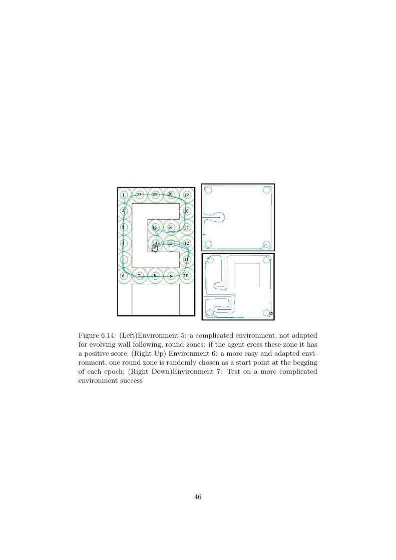
Figure 6.14: (Left)Environment 5: a complicated environment, not adaptedfor evolving wall following, round zones: if the agent cross these zone it hasa positive score; (Right Up) Environment 6: a more easy and adapted envi-ronment, one round zone is randomly chosen as a start point at the beggingof each epoch; (Right Down)Environment 7: Test on a more complicatedenvironment success

46

Figure 6.15: Environment 8, arrows gives the initial direction of the agentat the beginning of each epoch, big rounds are ”holes”, little rounds areobstacles; (Left) Environment for evolving a Left wall following (Right) En-vironment for evolving a Right wall following

the agent was positioned in the bottom right part of the environment andturned toward up. The big round on it’s right is a ”hole”, the agent cannotperceive it but if it goes on the round, it crash. This was done to force theagent to make Left wall following. The little rounds were added to teach theagent to continue following the wall even it there were obstacles on right.Then, when a good population was found, we re-evolve it on the secondEnvironment (figure 6.15 (Right)). Here we evolve agents able to performthe Right wall following. During the re-evolution, mutation was done only onthe second modula. In fact without this precaution, the agents could loosetheir ability to perform correctly the first task after the second evolution.

6.5.4 Define a sequence of Left and Right following

Here we will show first of all that the strategy is acceptable for any envi-ronment subset of EV (set of all visitable environment defined in equation6.12), if we use a random sequence of alternated WF-strategy. However, torender this strategy satisfying, we should define a good sequence.

Random sequence

We will consider again Environment 4. First we discretize our environmentin zone that the agent crosses in n life step (see grey and black rounds infigure 6.16) and that we will call n-life zone, and assume that the agentcould change WF-strategy every n-life zone, i.e one of this two possibility isselected randomly: continuing with the same WF-Strategy or change to theother WF-strategy.

47

Figure 6.16: Environment 4, subdivision in zone that could be crossed inn-life steps: round gray zones; round black zones: border zones between twosub-zones of the environment.

We can divide our environment in a set of sub-zone, that are set of n-lifezones:

Def 3

AB = SCP (A,B)

A′ = V A−AB

BC = SCP (B, C)

B′ = V B −BC

C ′ = V C −BC

with SCp(Cpi, Cpj) a set of connection points between Cpi, and Cpj as de-fined in equation 6.10, V Cpi the set of vicinity points as defined in definition1 and ”−” the normal substraction operator as defined by theory of set.The border points Bp (in black in figure 6.16) are n-life zones between twosub-zones, for example the border point 1 is between A′ and AB.Our exploration graph GE(E, V, Ψ) (see figure 6.19) will be defined as fol-lows: nodes are border points and edge between two nodes means that thereis a direct path between the corresponding border points, we give also theprobability of chousing such a path (considering that at each n-life zone theagent chooses randomly between continuing it’s WF-strategy or changes tothe other) and it’s length.The acceptability of the exploration strategy is insured by showing thatGE is strongly connected, i.e. by finding a circuit that visits all node.1 → 3 → 4 → 6 → 5 → 2 → 1 could be a possible circuit.But the average time needed to explore an Environment cannot be calcu-lated, as an agent could cycle indefinitely, for example 3 → 4 → 5 → 3.

48

Figure 6.17: Direct Exploration Graph of Environment 4; nodes: borderzone; edge between nodes a and b: path between a and b, label on edges:probability to chouse the corresponding path / length of the path.

In annex (see B)we give the demonstration that, for any Environment in-clude in the set of visitable Environments E′

V , a random sequence of WF-strategy is an acceptable exploration strategy (by showing that the explo-ration Graph of an environment En ⊂ E′

v i strongly connected) but not asatisfying one (by showing that an average time for visiting all rooms cannotby defined).

Fixed Time sequence

Another possibility could be to have a fixed time sequence. The idea wassimply to change WF-strategy every fixed m life steps. As we will see thismethods could give very good results and the exploration could be performedvery quickly sometimes, but the problem is that, at contrary to the randomsequence, here the acceptability is not insured.

For example, consider a strategy of fixed time sequence of alternated WF-strategies with m = 13 × n life steps on Environment 4 (see figure 6.16),with n the time needed to cross a gray (or a black) zone (the agent willchange WF-strategy after having crossed 13 round zones).If the agent begins on the the border zone 1 (black round), and do a Rightwall following, it will continue till arriving in the gray round positioned onthe Left of the border zone 2. Here it will change it’s WF-strategy and willcontinue forward by following the Left wall, till arriving back to the borderzone 1 where it will change again it WF-strategy, and so on it will cycle

49

indefinitely, and will never visit internal rooms B and C.

6.5.5 Results and critics

In this section we will present the results for the two different type of se-quence of WF-strategy that we have seen. The best individuals of the bestseed for both method have been tested on Environment 1,2,3. On figure 6.18we show the average percent of complete exploration compared to partialexploration, in 20’000 life steps.The table on right gives the average time (in thousand life steps) for anintegral exploration, and the square root of the variance. The test confirmswhat we have presented theoretically in the last section:

- With the fixed time sequence the probability to cycle is much higher.As we could see the rate of total exploration is much lower, particularyfor low values of m. The problem is, as we explained, that the agentcould indefinitely cycle. Instead using a random sequence, there isalways a possibility to explore integrally.

- However, for those that don’t cycle, the performance are better thanfor the random sequence. The average time for exploration is muchlower.

- The square root of variance of the the random sequence is very high.That confirms what we have theoretically shown, average time for therandom sequence is not insured.

- The value of n is negatively correlated with the success rate, for therandom sequence. That could be understood as follows. If the grayzone (that are defined by the value of n) on figure 6.13 are very big wecould have the same problem as for the fixed time sequence, i.e. theagent could indefinitely cycle.

To illustrated the relevance of the method using a random sequence, we givehere an example of a a successful test for each Environment. As we could seeagents using this method shows good ability to explore even complex envi-ronment. The only problem that we haven’t resolved yet is that sometimesthe agent doesn’t change wall when it changes WF-strategy, but simply turnand continue in in the other direction. To avoid this problem, that decreaseperformance in term of time, we have tried serval possible method: revolv-ing agents in a very big environment, to force them to go straight when thesensory inputs are low or use a third modula that is activate between twoWF-strategy and that is evolved for an obstacle avoidance, none succussedyet.In addition the crash rate is for the moment high: ∼ 15% indifferently forthe two methods and the different ambient. We haven’t include it in the

50

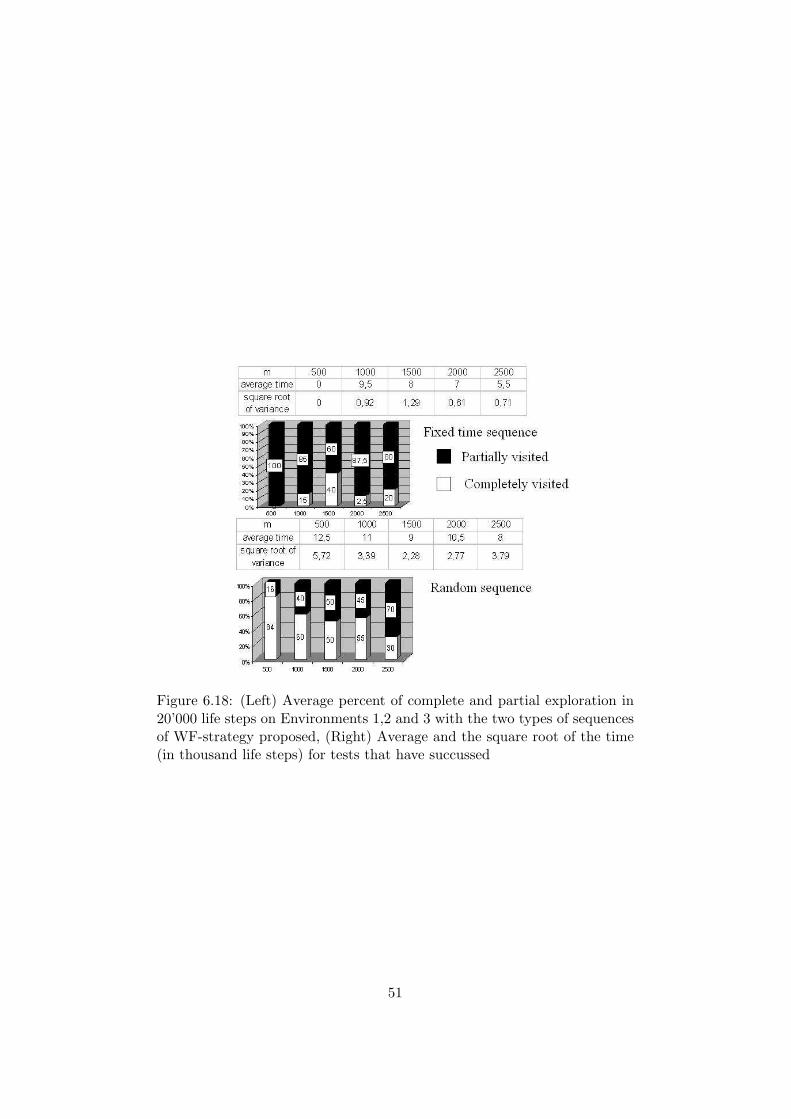
Figure 6.18: (Left) Average percent of complete and partial exploration in20’000 life steps on Environments 1,2 and 3 with the two types of sequencesof WF-strategy proposed, (Right) Average and the square root of the time(in thousand life steps) for tests that have succussed

51

Figure 6.19: Agent using a random sequence of WF-strategies, n = 1000 lifesteps, form top Left to Right: Environment 1,2 and 3, down: Environment4

statistics because it has nothing to do with the to types of strategy (norwith the value of m), it is simply a consequence of a problem that occursin the precise moment in which the agent changes from one WF-strategy tothe other: if the agent is in a corner, it crashes.

52

Chapter 7

Conclusion

Our research begun with the the human target following task, and we realizethat if a Robot had to follow a human, it had also to manage explorationwhen it loses its target.

We will discuss here our results in basis of what were our initial statements:Defining a robust strategy, using evolutionary robotics methods, to performthe exploration task with (Hybrid) reactive agents with two constraints: Space(The robot should be able to explore every part of the environment) and Time(It has to do it as fast as possible, avoiding as much as possible cycles).

Looking for particularities of realistic environment, we discovered the limi-tation of the simple reactive agents, and showed that they were unable toexplore environments that comport internal rooms (that is correlated withthe aliasing problem).Thus we have introduced three hybrid reactive agents: A reactive agent witha stochastic neuron, A reactive agent with an external memory encoding itsprecedent actions, An agent with a modular architecture.The conclusions we made are the following:

a A possibility to explore, and go out of cycles is to add some randomnesson the agent’s behavior. This method confronted us with a dilemma: ifthe behavior was very random, the agent was sometimes able to explorecorrectly but on the other hand its probability to crash increased.Istead, a lower level of randomes did’n’t permit reactive agents toexplore and go out of cycles.

b Another possibility was to add an information about the environment.We used an external memory coding the previous positions of theagent. Here the problem was the length of the memory, short mem-omry prevented only few cycles, and long memory introduced errorsbecause of the imprecise calculus of the postion. We have presented

53

also another experiment using two external memories with differentlength and we found agents which behavior was similar to agents withstochastic neuron. In fact by having two neurons using two externalmemories we augmented the variability of the agent in a intelligentway: the behavior became random when the agent returned in a placewhere it had been before or remained in the same area of the environ-ment.

c Finally we used a duplicated feedforward architecture with a modulathat chose at every life step which network was used. The idea herewas to traduce the indoor exploration as a sequence of Left and Rightwall following and evolve a distinct neural network for each task. Themost challenging problem was to define how the modula had to choosethe networks to be used. We have given in this project two veryeasy solution that still give good results: the modula chose randomlyevery m life step one of the two networks, or the two networks werealternatively selected every m life steps.

Our constraints were space and time. With all this new hybrid reactive agentwe have considerably augmented the performence in term of space: the newagent are in general able to explore more parts of the environment thanthe simple reactive. The most interesting was the one using the modulararchitecture with a rapid random sequence of Right and Left Wall Following.However the time needed to explore in this case wasn’t satisfying the agentcould do a lot of cycles before exploring all the environment.

Future Research

We obtained the most interesting results by using an agent with a modulararchitecture. One of our limitation was the high rate of crash. We thinkthat the problem is not inherent to the method, we should be able to avoidthe crash, changing may be the environment on which the agents are evolvedto perform the wall following. Our problem was that the agent learned howto follow wall on one side but didn’t learn to avoid the wall on the other side.

Another possible future work could be to introduce internal states. I thinkthat cupelling the modular method based on a sequence of Left and Rightwall following with a pro-active architecture able to perform the self-localizationtask could give interesting results. The self-localization ability could be usedto choose the right moment to change from one network to the other.

54

Bibliography

[1] S. Nolfi.(2000) Evorobot 1.1 user manual.http://gral.ip.rm.cnr.it/evorobot/simulator.html.

[2] K-Team S.A. Kephera robot(1998). Koala Version1.1 User manual.http://www.k-team.com.

[3] Miglino O., Lund H. and Nolfi S.(1995). Evolving mobile robots insimualting and real environments, Artificial Life, 2:417-434.

[4] Searle J.(1987). Minds and Brains without Programs , C. Blakemoreand S. Greenfield (eds.), Mindwaves (Oxford: Blackwell)

[5] Varela F.J., Rosch E., and Thompson E. (1991). The EmbodiedMind: Cognitive Science and Human Experience, Cambridge, MA: MITPress/Bradford Books.

[6] Cressant A.(1999) Etude in vivo des cellules de lieu, impliquees dans lamemoire spatiale, thesis repport

[7] Beer R.D. (1995). A dynamical systems perspective on agent-environment interaction, Artificial Intelligence, 72:173-215.

[8] Benhamou S., Sauve J.P. and Bovet, P. (1990). Spatial memory in largescale movements: Efficiency and limitations of the egocentric codingprocess. J. Theor. Biol., 145, 1-12.

[9] Olton D.S. (1982). Spatially organized behaviors of animal : behavioraland neurological studies. In : Spatial abilities. Developmental and phys-iological foundations, M. Potegal, Ed., New York : Academic Press,335-360.

[10] Beer R.D.(2001) The dynamics of active categorical perception in anevolved model agent. Behavioural and Brain Sciences, submitted.

[11] Braitenberg V. (1984). Vehicles: Experiments in Synthetic Psychology.MIT Press, Cambridge, Massachussets.

55

[12] Nolfi S. & Floreano D. (2000). Evolutionary Robotics, The biology, In-telligence, and Technology of Self- Organizing Machines, London, TheMIT Press/Bradford Books.

[13] Whitehead S.D. and Bellard D.H. (1991), Learing to perceive and actby trial and error, Machine Learning, 7:45-83

[14] O’Keefe J. and Nadel L. (1978). The hippocampus as a cognitive map.Oxford, U.K.: Oxford University Press. Workshop: Connectionist Rep-resentation. London: Springer Verlag

[15] Floreano D. and Mondada F. (1994), Automatic creation of an au-tonomus agent: genetic evolution of a neural-network driven robot, InD.Cliff,P.Husbands,J.Meyer and S.W. Wilson(Eds.), From Animals toAnimats 3: Proceedings of Third Conference on Simulation of Adapta-tive Behavior. Combrige, MA:MIT Press/Bradford Books.

[16] Bianco R., Caretti Massimiliano, Nolfi S.,(2003) Developing a Robotable to Follow a Human Target in a Domestic Environment,RoboCare:Proceedings of the First RoboCare Workshop. Rome: Edited byAmedeo Cesta.

[17] Miglino O., Denaro D., Tascini G., Parisini D.,(1998) Detour Be-havior in Evolving Robots: Are Internal Representations Neces-sary?,EvoRobots 1998: 59-70

[18] Etienne A. S., Joris-Lambert S., Reverdin B. and Teroni E. (1993).Learning to recalibrate the role of dead reckoning and visual cues inspatial navigation. Anim. Learn. Behav., 21, 266-280.

[19] McNaughton B.L., Chen L.L. and Markus E.J. (1991). ”Dead reckon-ing”, landmark learning, and the sense of direction: A neurophysiolog-ical and computational hypothesis. J. Cog. Neurosci., 3, 190-202.

[20] Nolfi S.,(2002) Evolving Robots able to Self-localize in the Environment:The Importance of Viewing Cognition as the Result of Processes Occur-ring at Different Time Scales, Connection Science (14) 3:231-244.

[21] De Croon G.,(2004) Pro-active agents with recurrent neural controllers,thesis repport

[22] Hill B., Best P. (1981) Effects of deafness and blindness on the spatialcorrelates of hippocampal unit activity in the rat. Exp. Neurol., 74, 204-217.

[23] Bahadori S., Iocchi L., Scozzafava L., (2003) People and Robot Lo-calization and Tracking through a Fixed Stereo Vision System, Robo-Care: Proceedings of the First RoboCare Workshop. Rome: Edited byAmedeo Cesta.

56

[24] Nolfi S. (1997) Using emergent modularity to develop control system formobile robotsAdaptative Beahvior, 3-4:343-364.

[25] Nolfi S. (1997) Evolving not trivial behavior on autonomous robots: Agarbage collecting Robot Robotics and Autonomous System, 22:187-198.

[26] Caprari G., Arras K.O. and Siegwart R. (2001) Robot Navigation inCentimeter Range Labyrinths. In Proceedings of the First InternationalConference on Autonomous Minirobots for Research and Edutainment,Heinz Nixdorf Institute, Paderborn, Germany.

[27] Johan Bos, Ewan Klein, and Tetsushi Oka. (2003) Meaningful conver-sation with a mobile robot. In Proceedings of the 10th Conference ofthe European Chapter of the Association for Computational Linguis-tics (EACL10), pages 71-74, Budapest

[28] Hartmann G. and Wehner R. (1995). The ants path integration system:a neural architecture. Biological cybernetics, 73:483-497

[29] Wehner R. Michel B. and Antonsen P. (1996). visual navigation in in-sects: Coupling of egocentric and geocentric information, The journalof experimental Biology, 199:129-140

[30] Kim D., Hallam J. C. T. (2000). Neural network approach to path in-tegration for homing navigation. In Meyer J. A., Berthoz A., FloreanoD., Roitblat H., S. W. Wilson (Eds.), From Animals to Animats 6 (pp.228-235). : MIT Press.

[31] Poucet B., Benhamou S. (1997). The neuropsychology of the spatialcognition in the rat. Critic. Rev. Neurobiol., 1 (2&3), 101-120.

57

Thanks

This thesis would not have been realized in one human life without thegreat help of my Supervisors Stefano Nolfi at the CNR in Rome and DarioFloreano at the EPFL in Lausanne. I would like to thank those how havehelped me during these four month: R. Bianco, for his innumerable hintand suggestions, Francesco Mondada for the precious help during my lastchaotic days of work, but also my colleague in CNR Gianluca Baldasarre,Marco, Luca, Davide, Massimiliano and Emiliano.Finally I would like to tanks Petra Krausz and Omar Shokur, for their helpduring the difficult writing process.A last special thanks for Romulus and Remus for having founded a city likeRome.

58

Appendix A

Graphs

Direct and Undirect Graph

A finite Direct (respectively Undirect) Graph G = (V, E,Ψ) is the tripletdefined by:

- A finite set V (|V | = n) who’s elements are called nodes

- A finite set E (|E| = m) who’s elements are edges

- A function Ψ : E −→ V x V , called function of incidence who asso-ciate for all edge e ∈ E an ordinate (respectively non ordinate) couple(u(e), v(e)) of nodes, where the node u(e) is the called initial extrem-ity of the edge e (respectively adjacent with e) and v(e) is the finalextremity of e (respectively adjacent with e).

Chain and Cycle

A chain is an alternated sequence of nodes and edges C = (u0, f1, u1, f2, u2, ..., uk−1, fk, uk)where ∀i ui ∈ V , fi ∈ E and fi = {ui−1, ui}

- A cycle is chain where the two extremity are the same node.

- A chain (or a cycle) is elementary if any node appear only once.

- A chain (or a cycle) is elementary if any edge appear only once.

- An undirect Graph is is acyclic if it no simple cycles.

Path and circuit

A path is an alternated sequence of nodes and edges C = (u0, f1, u1, f2, u2, ..., uk−1, fk, uk)where ∀i ui ∈ V and fi = (ui−1, ui) ∈ E.

- A circuit is a path where the two extremity are the same node.

- A direct graph is acyclic if it has no circuit.

59

Connectivity

Consider G = (V,E, ψ) an undirect graph, we define on V a relation ofconnectivity C as:

viCvj =

{vi = vj orThere is a chain between vi and vj

(A.1)

C is an equivalence relation: reflexive, symmetric and transitive. Classes ofequivalence of C define the connected components of G.

A graph G is connected ⇐⇒ G is composed by only one connected component(A.2)

Strong Connectivity

Consider G = (V, E, ψ) an direct graph, we define on V a relation of strongconnectivity CF as:

viCFvj =

{vi = vj orThere is a path between vi and vj , and a path between vj and vi.

(A.3)CF is an equivalence relation: reflexive, symmetric and transitive. Classesof equivalence of CF define the strong connected components of G.

A graph G is Strongly connected ⇐⇒G is composed by only one strong connected component

(A.4)

60

Appendix B

Demonstration

Acceptable strategy

We give here the demonstration that a random sequence of Left and Rightwall following is an acceptable strategy of exploration, for any environmentin E′

V .We have to show that: En ⊂ E′

V =⇒ the exploration graph GE(E, V, Ψ) isstrongly connected.

0. En ⊂ E′V

Justification: Hypothesis

1. En = {Cp1 ∪ Cp2 ∪ ... ∪ Cpn} and ∀Cpi, Cpj : Cpi ∩ Cpj = ∅J: 6.8

1.1 The set of points that could be visited by following elements of En,V En = {V Cp1 ∪ V Cp2 ∪ ... ∪ V Cpn}J: 1. and Def 1

2. ∀Cpi ∈ En,∃Cpj ∈ En[Cpi 6= Cpj and Rc(Cpi, Cpj)]J: 0. and 6.12

3. ∀Cpi ∈ En,∃Cpj ∈ En[Cpi 6= Cpj and (SCP (Cpi, Cpj) 6= ∅)]J: 2. and 6.11

4. SCP (Cpi, Cpj) ⊆ V Cpi

J: Definition 6.10

5. SCP (Cpi, Cpj) =⇒ V Cpi =(V Cpi∩¬SCP (Cpi, Cpj)

)∪SCP (Cpi, Cpj)

J: 4. and theory of set’s property : A = (A ∩ ¬B) ∪B if B ⊆ A

61

6. V En ={(

(V Cp1 ∩ ¬SCP (Cp1, Cpi)) ∪ SCP (Cp1, Cpi)) ⋃ (

(V Cp2 ∩¬SCP (Cp2, Cpj)) ∪ SCP (Cp2, Cpi)

) ⋃. . .

⋃ ((V Cpn ∩ ¬SCP (Cpn, Cpk)) ∪

SCP (Cpn, Cpk))}

J: 1. and 5.

7. V En ={C ′

1 ∪ C ′2 ∪ . . . ∪ C ′

n ∪ C1Ci ∪ C2Cj ∪ . . . ∪ CnCk

}

J: Def 3

Now we can continue the reasoning with graphs: we know that the WF-graph of En is connected (by definition of Environments ⊂ E′

V ). In additionwith proposition 7. we have a traduction of the environment V En in sub-zones. The border points that defines the nodes of the exploration graph aresimply the points between two sub-zones. We can show that the explorationgraph is strongly connected if the WF-graph is connected, by passing by anintermediary graph using the sub-zones as shown on figure B.1.We first traduce the undirect WF-Graph in a direct WF-Graph, by simplyduplicating any edge e in e′ and e′′. The non ordinate couple of nodes(u(e),v(e)) associated to e will be traduced in two ordinates couples of nodes((u(e), v(e)) and (v(e), u(e))) associated to e′ and e′′. The correspondingdirect graph is strongly connected.If the directed WF-graph is strongly connected the sub-zone graph is stronglyconnected, and by so the exploration graph is strongly connected, as thenodes are the points between two sub zone and edges are path between twoborder zone. The existence of the path is insured by the fact that we havebased the exploration graph on sub-zones graph, path between two bordernodes is the corresponding node of the sub-zone graph, for example the pathbetween the border node i and j is CpiCpj .

Thus the exploration graph, for the exploration strategy based on a randomsequence of Right and Left wall following is strongly connected.

Non satisfying strategy

We want to show here that an average time for exploring an environmentintegrally by using a random sequence of Right and Left following is notinsured, and by so that the strategy is not satisfying.

The average time for exploring could be found by calculating the averagelength of the Exploration graph (see figure 6.19).The average length is the average of the Expected Value of all the possiblepaths:

62

Figure B.1:

1n

n∑

i=0

E(Pathi)

with n the number of possible path and E(pathi) given by:

E(pathi) =1m

m∑

j=0

λ(edgej)× P (edgej)

with m the number of edges for the corresponding path, λ(edge) and P (edge)respectively the length and the probability of the the edge (as defined in ourexploration graph on figure 6.19).As our graph is cyclic, the number of possible path n → ∞, and thus theaverage length is undefined: the strategy is not satisfying.

63