Control System Modeling and Design for a

Mars Flyer, MACH-1 Competition

Gabriel Hugh Elkaim

∗University of California, Santa Cruz

Ji-Wung Choi, Daniel Garalde, and Mariano Lizarraga†

Mars science missions would benefit from the ability to acquire high

resolution images of the Martian surface, as well as sensor coverage from

other sensors. A robotic aircraft on Mars has been proposed to carry these

instruments. The atmosphere and weak Martian gravity make the plane

equivalent to a very high altitude aircraft on the Earth. The MACH-1

challenge is a design contest to model, simulate, and design the control

system for this future Mars flyer. The design specifications are used to cre-

ate a SIMULINK full six degree of freedom model, which is validated with

open loop simulations. Trim conditions are used to generate perturbation

models for control loop design, and output regulator linear quadratic reg-

ulator design is used to generate a gain matrix for straight and level flight.

The generated model is unstable, and the control design developed cannot

stabilize the non-linear model.

Nomenclature

x, y, z Position

u, v, w Forward, side, vertical speed

X, Y, Z Frame axis

φ, θ, ψ Angular states

∗Assistant Professor, Department of Computer Engineering, UCSC, 1156 High St., Santa Cruz, CA,95064, USA.†Graduate Student, Department of Computer Engineering, UCSC, 1156 High St., Santa Cruz, CA, 95064,

USA.

p, q, r Angular rates

α Angle of attack

β Sideslip angle

A Aspect Ratio

b Wing semi-span, m

c Section chord

Vtas Air speed

Cx, Cy, Cz Force coefficients in the x, y or z direction

CD Drag coefficient

CL Lift coefficient

Cm Pitching moment coefficient

Cp Section pressure coefficient

CY Side Force

Cl Roll Moment

Cn Yaw Moment

D Drag, N

L Lift, N

M Pitching moment about quarter chord, N-m

Re Reynolds number

S Area, m2

λ Wing taper ratio

Λs Wing sweep angle

m Mass, kg

I Inertia, kg·m2

dt Sampling time, s

x, y, z Error signal for the position x, y, z

T Air temperature on Mars, K

a Speed of sound on Mars, m/s

P Air pressure on Mars, Pa

ρ Air density on Mars, kg/m3

h Height, m

Subscript

T Tail

W Wing

RV sym Symmetric ruddervator

RV diff Differential ruddervator

Superscript

B Body drame

W Wind frame

I. Introduction

In 1964, the Mariner 4 NASA spacecraft was the first to focus specifically on Mars.

Since then, NASA has flown a number of missions to photograph, map, and study Mars.

Mars research has many motivations, including searching for traces of life on Mars, and

determining if Mars could support human occupants in the future. Mars missions have

included crafts which photograph mars from space and robotic rovers that can traverse the

Martian surface, both which send a wealth of data to Earth. However, one potential venue

for Mars exploration that has not yet been exploited is the use of a robotic aircraft designed

to fly in the thin atmosphere above the Martian soil. Such an aircraft could be used for,

among other things, aerial imaging of Mars. Mathworks sponsored the MACH-1 competition

by which student teams compete to build a control system for a proposed Mars aircraft.

Prior to the competition, designers use simulations to generate accurate aerodynamic

data for the proposed aircraft. The following parameters are thus supplied to each student

team.

• Aircraft aerodynamic model

• Aircraft mass properties

• Engine model

• Sensor Model

• Atmospheric Model

This report focuses on our team’s work to implement a MATLAB system model and to design

the control system for the proposed Mars aircraft. From the supplied system parameters,

we use a 6 degree-of-freedom model for the aircraft, and build SIMULINK models for the

engine, actuators, sensors (including added noise), and Martian atmosphere. These models

are described in detail in Sections 2-3. Most likely due to a modeling error, the resulting

system is unstable. This report describes our control design approach assuming a stable,

and trimmed model.

Figure 1. Image of the ARES flyer over simulated Martian terrain.

II. Aircraft Model Specifications

This section presents a detailed implementation of the 6-DOF model for the ARES air-

craft.

II.A. 6-DOF Aircraft Model

The derivation of the equations of motion for a 6-DOF aircraft model to be used as a plant in

the control system design was done in two steps. The first step was formulating the equations

of motion for the aircraft, treated as a rigid body. The second step was the computation

of aerodynamic, gravitational and propulsive forces that act upon the aircrafts body. The

aerodynamic and propulsive forces are specific to the aircraft to be modeled and depend

directly on the airfoil, aircraft geometry, mass dispersion, and engine characteristics.

In the following subsections, the development of the equations of motion for the aircrafts

linear and angular dynamics are developed.

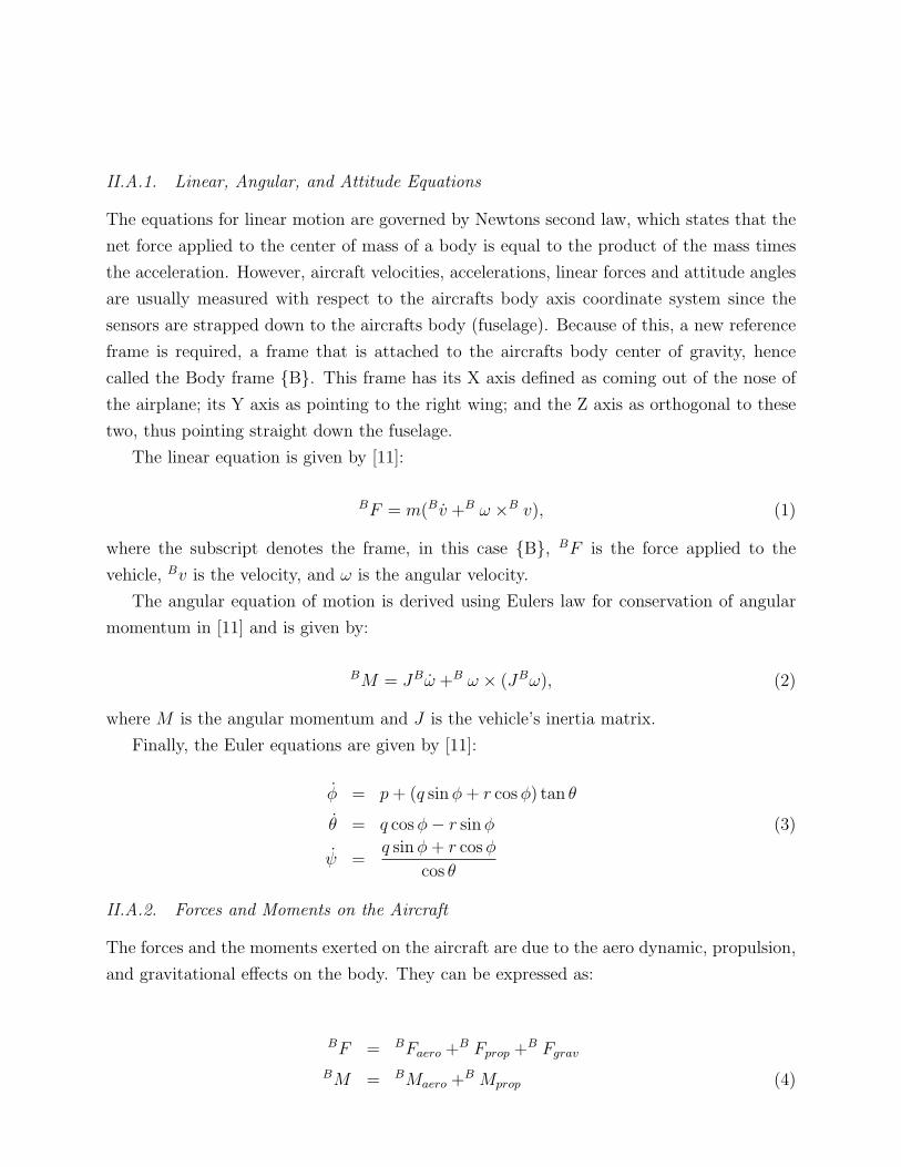
II.A.1. Linear, Angular, and Attitude Equations

The equations for linear motion are governed by Newtons second law, which states that the

net force applied to the center of mass of a body is equal to the product of the mass times

the acceleration. However, aircraft velocities, accelerations, linear forces and attitude angles

are usually measured with respect to the aircrafts body axis coordinate system since the

sensors are strapped down to the aircrafts body (fuselage). Because of this, a new reference

frame is required, a frame that is attached to the aircrafts body center of gravity, hence

called the Body frame {B}. This frame has its X axis defined as coming out of the nose of

the airplane; its Y axis as pointing to the right wing; and the Z axis as orthogonal to these

two, thus pointing straight down the fuselage.

The linear equation is given by [11]:

BF = m(B v +B ω ×B v), (1)

where the subscript denotes the frame, in this case {B}, BF is the force applied to the

vehicle, Bv is the velocity, and ω is the angular velocity.

The angular equation of motion is derived using Eulers law for conservation of angular

momentum in [11] and is given by:

BM = JBω +B ω × (JBω), (2)

where M is the angular momentum and J is the vehicle’s inertia matrix.

Finally, the Euler equations are given by [11]:

φ = p+ (q sinφ+ r cosφ) tan θ

θ = q cosφ− r sinφ (3)

ψ =q sinφ+ r cosφ

cos θ

II.A.2. Forces and Moments on the Aircraft

The forces and the moments exerted on the aircraft are due to the aero dynamic, propulsion,

and gravitational effects on the body. They can be expressed as:

BF = BFaero +B Fprop +B FgravBM = BMaero +B Mprop (4)

II.A.3. Aerodynamic Forces and Moments

The aerodynamic forces and moments that act upon an aircraft are produced by the relative

motion of the aircraft with respect to the air mass (the airspeed). Mathematically, the

aerodynamic forces and moments terms are determined by using a first-order Taylor series

expansion around the aircraft trimmed operating point. Each term in the series is a partial

derivative of the forces and moments with respect to the aerodynamic variables. These

aerodynamic variables are given by the deflection of the aileron, and the left and right

ruddervators.

Let the angle of attack α be the angle between the projection of the airspeed vector to

the XZ body plane and the Xbody axis. Also let the sideslip angle β, be the angle between

the projection of the airspeed vector to the XY body plane and the X body axis. Since the

forces and moments depend on the airspeed, a new co- ordinate frame must be introduced.

In this new coordinate frame, denoted as {W}, the X axis is aligned with the winds velocity

vector (W ). The rotation matrix BWR, which rotates a vector from {W} to {B}, is given

in [11], and thus equation (4) is rewritten as:

BF = BWR

WFaero +B Fprop +B FgravBM = B

WRWMaero +B Mprop (5)

For simplicity, the aerodynamic forces and moments acting on the aircraft are defined

in terms of dimensionless aerodynamic coefficients that, as expected, depend on the control

surfaces deflection, the aerodynamic angles α and β, and the angular rates (p, q, r). The

forces and moments expressed in terms of the dimensionless aerodynamic coefficients are

derived in [11] and shown in equation (6) for easy reference.

WF = qS[CD CY CL]T

WM = qS[Clb Cmc Cnb]T , (6)

where q is the dynamic pressure, S is the wing reference area, c is the wing chord and b is

the wingspan.

The numerical values for the dimensionless aerodynamic coefficients required by equation(6)

were given in the initial problem specifications and were, in general, described as functions of

mach number and angle of attack α. Section III.B describes how this functions were actually

implemented in the Model.

II.A.4. Gravitational and Propulsive Forces and Moments

Gravitational forces act on the rigid body but generate no moments since the forces are

assumed to act at the center of gravity. The gravitational forces are resolved in the local

reference frame {L} and are given by:

BFgrav =BL R[0 0 mg]T , (7)

where BLR is The rotation matrix which rotates a vector from {L} to {B}, m is the aircraft’s

mass and g is the gravity constant.

The propulsive forces and moments are exerted in {B} and can be stated as:

BFprop = [Px Py Pz]T

BMprop = [Pl Pm Pn]T , (8)

where each of the scalars Pi represent forces or moments due to the aircrafts thrust. Since

for the aircraft being modeled the engine thrust axis coincides with the X axis of {B}, then

the thrust projections Py and Pz are assumed to be zero.

II.A.5. Dimensionless Aerodynamic Coefficients

For the The aerodynamic coefficients described in equation (6) are given by:

CD = CDbasic + ∆CDRV sym + ∆CDdyn

CY = CYbasic + ∆CYRV diff + ∆CYAil + ∆CYdyn (9)

CL = CLbasic + ∆CLRV sym + ∆CLdyn ,

Cl = (Clbasic + ∆ClRV diff + ∆ClAil + ∆Cldyn) +[

0 ∆Zcg −∆Ycg

]CX

CY

CZ

Cm = (Cmbasic + ∆CmRV sym + ∆Cmdyn) +

[−∆Zcg ∆Xcg

] CX

CZ

(10)

Cn = (Cnbasic + ∆CnRV diff + ∆CnAil + ∆Cndyn) +[

∆Ycg −∆Xcg 0]·

CX

CY

CZ

where

∆CDdyn = 0

∆CYdyn = 0 (11)

∆CLdyn = 0

∆Cmdyn = −20q

(c/(2Vtas))

∆Cndyn = (−0.14 · p− 1.2 · r)/(b/(2Vtas)) (12)

∆Cldyn = (−1 · p+ 0.2 · r)/(b/(2Vtas)),

as specified by the competition furnished information; the coefficients with the Ail subscript

are function of mach number, α, and aileron defflection; the coefficients with the subscript

basic are functions of mach number and α; the coefficients with RVsym subscript are functions

of mach number, α, and symetric ruddervator RVsym, which is given by:

RVsym =RVleft +RVright

2, (13)

the coefficients with the subscript RVdiff are functions of mach number, α, and differential

ruddervator RVdiff , which is given by:

RVdiff =RVleft −RVright

2, (14)

CX

CZ

=

− cosα sinα

− sinα − cosα

CD

CL

, (15)

and

∆XCG = −(FS − FSref )/c

∆YCG = +(BL−BLref )/b (16)

∆ZCG = −(WL−WLref )/c.

At the beginning of the competition, The Mathowrks provided a set of lookup tables

with information obtained for the ARES vehicle that allowed to compute all the previously

mentioned coefficients.

II.A.6. Engine and Actuator Models

The mathematical model of the aircrafts engine required for the 6-DOF model needed to

reflect the relationship between the throttle commanded by the autopilot, and the thrust

exerted to the aircrafts body expressed in Newtons. For this, a simple first order system was

used as described in the competition furnished information.

For the actuators’ models a second order non-linear model was used as specified by the

competition furnished information.

II.B. Mass Properties

CG offsets ∆XCG, ∆YCG, and ∆ZCG are given by:

∆XCG = −FS − FSrefc

(17)

∆YCG = −BL−BLrefb

(18)

∆ZCG = −WL−WLrefc

(19)

Where aerodynamic reference fuselage station FSref , CG fuselage Station FS, aerody-

namic reference buttline BLref , CG buttline BL, aerodynamic reference waterline WLref ,

and CG waterline WL, initial mass minit and initial inertia Iinit are specified in Appendix.

II.C. Engine Model

Thrust time constant Tthrust and thrust scale factor Kthrust have the following relationship:

Tthrust = KthrustUthrust (20)

Where Uthrust is thrust command.

Note that:

dm

dt=TthrustVeffex

(21)

Where effective exhaust velocity Veffex, thrust alignment Athrust, and CG relative thrust

lever arm lthrust are specified in Appendix.

II.D. Sensor Model

II.D.1. Error Model for x and y

Error model for x is represented as the state-space model as following:

x = Ax + Bw (22)

y = Cx + Dw (23)

Where

x = (x, ˙x, ax,bias, Vx,wnd)T (24)

w = (N(0, ANP ), N(0, XNP ), N(0, V NP ))T (25)

y = (x, ˙x, Vx,wnd)T (26)

Where ax,bias is error signal for the acceleration bias. Vx,wnd is error signal for the wind

component in the x direction. Acceleration variance ANP , position variance XNP , velocity

variance V NP , and the discrete time model state matrices A, B, C, and D with dt = 0.02

are specified in Appendix.

Error Model for y is obtained by replacing the state x and the output y by

x = (y, ˙y, ay,bias, Vy,wnd)T (27)

y = (y, ˙y, Vy,wnd)T (28)

into Equation (22) and (23).

II.D.2. Error Model for z

Error model for z is represented as the state-space model as following:

z = Az + Bw (29)

y = Cz + Dw (30)

Where

z = (z, ˙z, az,bias, Vz,wnd)T (31)

w = (N(0, ANP ), N(0, ZNP ), N(0, V NP ), N(0, ALTNP ))T (32)

y = (z, ˙z, Vz,wnd)T (33)

Where acceleration variance ANP , position variance ZNP , velocity variance V NP , al-

titude variance ALTNP , and the discrete time model state matrices A, B, C, and D with

dt = 0.02 are specified in Appendix.

II.D.3. Error Model for Angular States

Error model for φ is represented as the state-space model as following:

x = Ax + Bw (34)

y = Cx + Dw (35)

Where

x = (φ, pbias)T (36)

w = (N(0, RATENP ), N(0, ANGNP ))T (37)

y = (φ)T (38)

Where pbias is error signal for the angular rate bias. Angular rate variance RATENP ,

angle variance ANGNP , and the discrete time model state matrices A, B, C, D with

dt = 0.02 are specified in Appendix.

Error Model for θ or ψ are obtained by replacing the state x and the output y into

Equation (34) and (35).

II.E. Atmospheric Model

The model presented in this paper uses a simplse curve-fit empirical model of the temper-

ature, pressure, density and speed of sound on Mars. This model was derived from Mars

Global Surveyor Data from 1996. Temperature T , speed of sound a, pressure P and density

ρ are given as follows:

T = 249.75− 0.00222h [K] (39)

a =√γRmT [m/s] (40)

P = 699e−0.00009h [Pa] (41)

ρ = P/(RmT ) [kg/m3] (42)

where γ = 1.29 and Rm = 191.8 [(N ·m)/(kg ·K)].

III. Aircraft Model Development

Inputs to the aircraft model are assigned as follows:

III.A. Aerodynamic Model

Wing semi-span b, normalized section chord c, area S are given by:

b = 6.25 [m] (43)

c = 1.25 [m] (44)

S = 7 [m2] (45)

The normalized angular rates are given by:

p =pb

2Vair[rad/s] (46)

q =qc

2Vtas[rad/s] (47)

r =rb

2Vtas[rad/s] (48)

III.A.1. Longitudinal Coefficients

Correct moment coefficients for CG offset are obtained by:CxCz

=

− cosα sinα

− sinα − cosα

CDCL

(49)

Cm = (Cmbasic + ∆CmRVsym + ∆Cmdyn) +[−∆ZCG ∆XCG

]CxCz

(50)

Where CG offsets ∆XCG, ∆YCG, and ∆ZCG are represented in Equation (17), (18), and

(19). Force coefficients are obtained by:

CL = CLbasic + ∆CLRVsym + ∆CLdyn (51)

CD = CDbasic + ∆CDRVsym + ∆CDdyn (52)

Where basic coefficients CLbasic , CDbasic , and Cmbasic are computed by looking up tables

with information obtained for the ARES vehicle:

CLbasic = 2DLookup(mach.basic, alphasched.basic, CL.basic,M, α) (53)

CDbasic = 2DLookup(mach.basic, alphasched.basic, CD.basic,M, α) (54)

Cmbasic = 2DLookup(mach.basic, alphasched.basic, Cm.basic,M, α) (55)

Where, for the basic coefficients, mach number abscissa vector mach.basic, angle of at-

tack abscissa vector alphasched.basic, lift coefficient table CL.basic, drag coefficient table

CD.basic, and pitching moment coefficient table Cm.basic are specified by the CFI (com-

petition furnished information) that the Mathworks provided. Symmetric ruddervator coef-

ficients ∆CLRVsym , ∆CDRVsym , and ∆CmRVsym are also computed by looking up tables:

∆CLRVsym = 3DLookup(mach.drvs, alphasched.drvs, drvssched, CL.drvs,M, α,RVsym)

(56)

∆CDRVsym = 3DLookup(mach.drvs, alphasched.drvs, drvssched, CD.drvs,M, α,RVsym)

(57)

∆CmRVsym = 3DLookup(mach.drvs, alphasched.drvs, drvssched, Cm.drvs,M, α,RVsym)

(58)

Where, for the symmetric ruddervator coefficients, mach number abscissa vector mach.drvs,

angle of attack abscissa vector alphasched.drvs, symmetric ruddervator abscissa vector

drvssched, lift coefficient table CL.drvs, drag coefficient table CD.drvs, and pitching mo-

ment coefficient table Cm.drvs are specified by the CFI. Symmetric ruddervator RVsym is

represented in Equation (13).

Dynamic coefficients are obtained by:

∆CLdyn = CL.dyn (59)

∆CDdyn = CD.dyn (60)

∆Cmdyn = Cm.q · q (61)

Where, for the dynamic coefficients, lift coefficient table CL.dyn, drag coefficient table

CD.dyn, and dCmdq

table Cm.q are specified by the CFI.

III.A.2. Lateral Coefficients

Correct moment coefficients for CG offset are obtained by:

Cl = (Clbasic + ∆ClRV diff + ∆ClAil + ∆Cldyn) +[

0 ∆Zcg −∆Ycg

]CX

CY

CZ

Cn = (Cnbasic + ∆CnRV diff + ∆CnAil + ∆Cndyn) +[

∆Ycg −∆Xcg 0]·

CX

CY

CZ

CY = CYbasic + ∆CYRV diff + ∆CYAil + ∆CYdyn (62)

Where basic coefficients CYbasic , Clbasic , and Cnbasic are obtained by:

CY β = 2DLookup(mach.basic, alphasched.basic, CY B.basic,M, α) (63)

CYbasic = CY β · β (64)

Clβ = 2DLookup(mach.basic, alphasched.basic, ClB.basic,M, α) (65)

Clbasic = Clβ · β (66)

Cnβ = 2DLookup(mach.basic, alphasched.basic, CnB.basic,M, α) (67)

Cnbasic = Cnβ · β (68)

(69)

Where, for the basic coefficients, dCYdβ

table CY B.basic, dCldβ

table ClB.basic, and dCndβ

table

CnB.basic are specified by the CFI.

Differential ruddervator coefficients ∆CYRVdiff , ∆ClRVdiff , and ∆CnRVdiff are obtained by:

∆CYRVdiff = 3DLookup(mach.drva, alphasched.drva, drvssched, CY 0.drva,M, α,RVdiff )

(70)

∆ClRVdiff = 3DLookup(mach.drva, alphasched.drva, drvssched, Cl0.drva,M, α,RVdiff )

(71)

∆CnRVdiff = 3DLookup(mach.drva, alphasched.drva, drvssched, Cn0.drva,M, α,RVdiff )

(72)

Where, for the differential ruddervator coefficients, mach number abscissa vector mach.drva,

angle of attack abscissa vector alphasched.drva, differential ruddervator abscissa vector

drvssched, side force coefficient table CY 0.drva, rolling moment coefficient table Cl0.drva,

and yawing moment coefficient table Cn0.drva are specified by the CFI. Differential rudder-

vator RVdiff is represented in Equation (14).

Aileron coefficients are obtained by:

∆CYAil = 3DLookup(mach.dail, alphasched.dail, dailsched, CY 0.dail,M, α,Ail) (73)

∆ClAil = 3DLookup(mach.dail, alphasched.dail, dailsched, Cl0.dail,M, α,Ail) (74)

∆CnAil = 3DLookup(mach.dail, alphasched.dail, dailsched, Cn0.dail,M, α,Ail) (75)

Where, for the aileron coefficients, mach number abscissa vector mach.dail, angle of attack

abscissa vector alphasched.dail, aileron abscissa vector dailsched, side force coefficient table

CY 0.dail, rolling moment coefficient table Cl0.dail, and yawing moment coefficient table

Cn0.dail are specified by the CFI.

Dynamic coefficients are obtained by:

CYdyn = CY 0.dyn (76)

Cldyn =2Vtasb

(Cl0.p · p+ Cl0.r · r) (77)

Cndyn =2Vtasb

(Cn0.p · p+ Cn0.r · r) (78)

Where side force coefficient table for the dynamic coefficients CY 0.dyn, d(Cl0)dp

table Cl0.p,d(Cl0)dr

table Cl0.r, d(Cn0)dp

table Cn0.p, and d(Cn0)dr

table Cn0.r are specified by the CFI.

III.B. Simulink Implementation

Figure 2 presents a top-level view of the implemented Simulink Model. The model consists of

four main subsystems: The actuators model, the 6-DOF model as described in the previous

section, the sensor model and the atmosphere.

Figure 2. Simulink Model Overview

1The actuator model (Figure 3) makes use of a readily available Simulink block in the

Aerospace blockset: the second order linear actuator.

Figure 3. Actuator Model

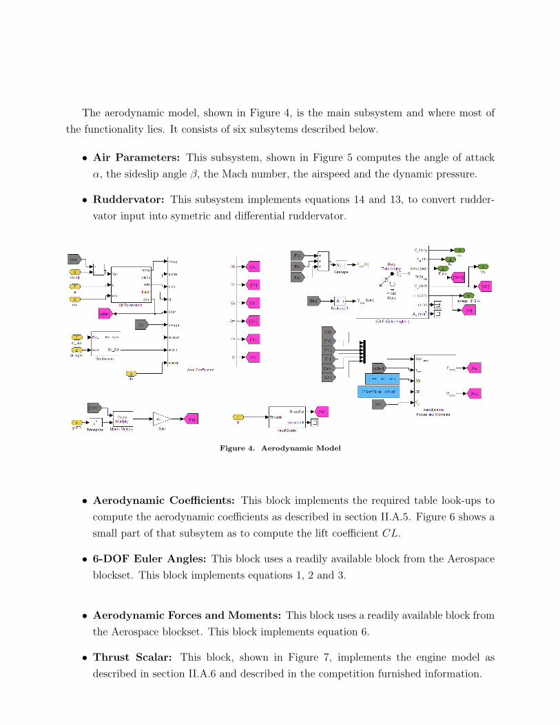
The aerodynamic model, shown in Figure 4, is the main subsystem and where most of

the functionality lies. It consists of six subsytems described below.

• Air Parameters: This subsystem, shown in Figure 5 computes the angle of attack

α, the sideslip angle β, the Mach number, the airspeed and the dynamic pressure.

• Ruddervator: This subsystem implements equations 14 and 13, to convert rudder-

vator input into symetric and differential ruddervator.

Figure 4. Aerodynamic Model

• Aerodynamic Coefficients: This block implements the required table look-ups to

compute the aerodynamic coefficients as described in section II.A.5. Figure 6 shows a

small part of that subsytem as to compute the lift coefficient CL.

• 6-DOF Euler Angles: This block uses a readily available block from the Aerospace

blockset. This block implements equations 1, 2 and 3.

• Aerodynamic Forces and Moments: This block uses a readily available block from

the Aerospace blockset. This block implements equation 6.

• Thrust Scalar: This block, shown in Figure 7, implements the engine model as

described in section II.A.6 and described in the competition furnished information.

Figure 5. Air Parameters Subsystem

Figure 6. Table Look-Up For Aeordynamic Coefficients Calculation

IV. Aircraft Model Verification and Validation

The simulink model was validated by testing blocks with known inputs and verifying that

the outputs were consistent with the specification data provided by the MACH-1 RFP. For

instance, the Mars atmosphere model, detailed in Section II, shows that Mach number, a,

Temperature, T , and density, ρ, are all functions only of altitude. Thus, the atmospheric

data was hand calculated at 1000 m., and the outputs compared to the output of the block

with a constant 1000 injected at the input.

This was done for each block where it was possible to do so. For validating the Mars flyer

model as a whole, an open loop simulation was run with parameters near their trim values

for aileron, ruddervators, and throttle. Given an initial condition of 1000 m. altitude, 150

m/s velocity, and a heading of due north, the model demonstrated an exaggerated phugoid

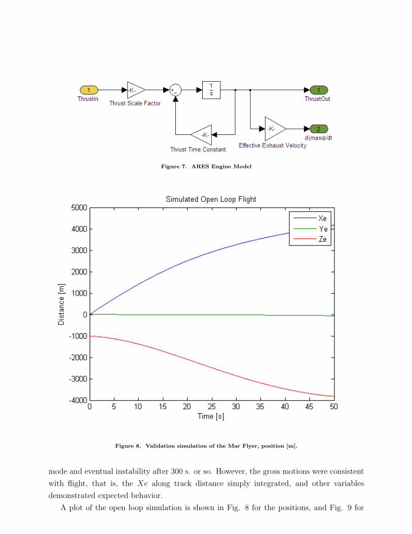
Figure 7. ARES Engine Model

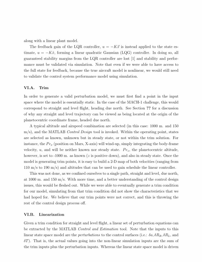
Figure 8. Validation simulation of the Mar Flyer, position [m].

mode and eventual instability after 300 s. or so. However, the gross motions were consistent

with flight, that is, the Xe along track distance simply integrated, and other variables

demonstrated expected behavior.

A plot of the open loop simulation is shown in Fig. 8 for the positions, and Fig. 9 for

Figure 9. Validation simulation of the Mar Flyer, Euler angles [◦].

the Euler angles.

V. Control Design Specifications

The MACH-1 challenge has as its goal the design of a control loop, deliverable in ANSI

standard C code, running at a control loop rate of 50Hz. While most of the team effort was

expended in developing the Mars flyer non-linear model, some effort was made at defining

the control problem.

The desired trajectory for the Mars flyer is straight and level flight (constant altitude

and heading). The first thing to note is that without loss of generality, the control trajectory

can be considered simply to be heading North from the equator at a given altitude. This is

because a new set of path coordinates can be defined on the current segment of the trajectory,

with the origin at the initial waypoint, and the heading pointed towards the next waypoint.

In these path coordinates, the vehicle appears to be flying due north from the origin of

the planetocentric coordinate frame. Note that oblateness of Mars can introduce distortion

errors, but for the purpose of control design, this is more than sufficient.

In terms of control design specifications, only a few criteria were used. The first was

stability: the Mars flyer should track its constant altitude and heading trajectory without

diverging from it. Note that the linearized model of the flyer is unstable, and the non-linear

model shows instability in both the phugoid and dutch roll modes. Thus feedback control

will be required, at minimum, to stabilize the aircraft.

The other criteria are path regulation: the Mars flyer should be able to reacquire the

trajectory line from a cross track error or altitude error of 10 m. regardless of the cause.

This indicates robustness, and a disturbance rejection of an impulsive disturbance, requiring

a type 1 system. Given the maneuverability of the craft, the time to recover to within 1 m.

of the desired trajectory from an impulsive disturbance should be less than 60 seconds. This

places a bound on the rise time of the closed loop (linearized) system, which consequently

determines a lower limit of the modal natural frequencies of 0.03 rad/s. Note that this also

implies a final steady state error of less than 1 m. This determines the minimum loop gain

for the system, or requires the addition of integral control.

While these criteria are fairly gentle, they pose a challenge as the system is non-linear.

As such, the linear tools will only help us get so far. Using the linear analysis tools, we will

make sure that the linear system response satisfies the criteria. However, we will use the

simulation to validate that the control system performs as well on the non-linear full 6DoF

model.

VI. Control Design Development

The control design for the MACH-1 design contest presents both challenges in terms

of technical execution, as well as an opportunity to learn to apply the control techniques

to a realistic system. The control strategy employed by our team was a simple three part

approach. First, the model was trimmed using the SIMULINK tools about the nominal

trajectory, then a linear model perturbation model was extracted, also using the SIMULINK

tools.

Using the linear model, and assuming the entire state was available, a linear quadratic

regulator (LQR) is designed to reject all disturbances from the ARES flyer (such as wind

gusts, mismodeling, sensor or actuator noise, etc.). Unfortunately, the entire state is not

available for an LQR design, and thus an estimator is required as well. In order to design

the estimator, a Kalman filter is designed to estimate the state given the measured outputs

along with a linear plant model.

The feedback gain of the LQR controller, u = −K~x is instead applied to the state es-

timate, u = −Kx, forming a linear quadratic Gaussian (LQG) controller. In doing so, all

guaranteed stability margins from the LQR controller are lost [1] and stability and perfor-

mance must be validated via simulation. Note that even if we were able to have access to

the full state for feedback, because the true aircraft model is nonlinear, we would still need

to validate the control system performance model using simulation.

VI.A. Trim

In order to generate a valid perturbation model, we must first find a point in the input

space where the model is essentially static. In the case of the MACH-1 challenge, this would

correspond to straight and level flight, heading due north. See Section ?? for a discussion

of why any straight and level trajectory can be viewed as being located at the origin of the

planetocentric coordinate frame, headed due north.

A typical altitude and airspeed combination are selected (in this case: 1000 m. and 150

m/s), and the MATLAB Control Design tool is invoked. Within the operating point, states

are selected as known, unknown but in steady state, or not within the trim solution. For

instance, the Pex (position on Mars, X-axis) will wind-up, simply integrating the body-frame

velocity, u, and will be neither known nor steady state. Pez, the planetocentric altitude,

however, is set to -1000 m. as known (z is positive down), and also in steady state. Once the

model is generating trim points, it is easy to build a 2-D map of both velocities (ranging from

110 m/s to 190 m/s) and altitudes that can be used to gain schedule the linear controller.

This was not done, as we confined ourselves to a single path, straight and level, due north,

at 1000 m. and 150 m/s. With more time, and a better understanding of the control design

issues, this would be fleshed out. While we were able to eventually generate a trim condition

for our model, simulating from that trim condition did not show the characteristics that we

had hoped for. We believe that our trim points were not correct, and this is throwing the

rest of the control design process off.

VI.B. Linearization

Given a trim condition for straight and level flight, a linear set of perturbation equations can

be extracted by the MATLAB Control and Estimation tool. Note that the inputs to this

linear state space model are the perturbations to the control surfaces (i.e.: δa, δRR, δRL, and

δT ). That is, the actual values going into the non-linear simulation inputs are the sum of

the trim inputs plus the perturbation inputs. Whereas the linear state space model is driven

only by the perturbation inputs centered around 0.

The linearization process produces a model that has 19 states, with four inputs (the

perturbations on the control surfaces) and six outputs (the planetocentric positions and

three euler angles). Note that we could have included the three rates and the three body

fixed velocities as well, but we chose to ignore those outputs, as they do not come into the

control problem. In the end, we feel that the linearized model is not a very good one, and

does not stabilize well using LQR control.

Looking at the eigenvalues of the linearized model, we can see several things. Firstly,

there are some very fast modes that are quite well damped and come from the actuator

dynamics. For the sake of control design, these can be safely ignored. Looking closer at the

origin, there are three poles on the origin, indicating straight integration (rigid body mode

of the vehicle). There are damped oscillations, which correspond to the short period mode,

and a few unstable, but very slow modes (indicating dutch roll and phugoid modes). The

eigenvalues and damping ratios of the linear system are listed in Table 1.

Eigenvalue Damping Frequency (rad/s)

0.00065 -1 0.00065

0.00056 -1 0.00056

0 (x3) 0

-0.00104 1 0.00104

−0.00112± 0.0642j 0.0175 0.0642

−0.56± 2.82j 0.195 2.87

-5 1 5

−132± 135j (x3) 0.7 188

-1070 1 1070

-1380 1 1380Table 1. Damping characteristics of linearized system

VI.C. LQR control

With a trimmed point, and a linearized perturbation model, a regulator is needed to keep

the vehicle tracking the designed path (in this case, straight and level). The first thing to

note is that there are only three output variables that need to be regulated: δY, δZ, and

δΨ. That is, given that we have rotated out path dynamics such that we are the nominal

altitude and heading required, a local coordinate frame on that path will have the aircraft

flying along the x-axis, and hold the cross track error, altitude error, and heading error to 0.

Given this output regulator structure, a linear quadratic regulator (LQR) design is very

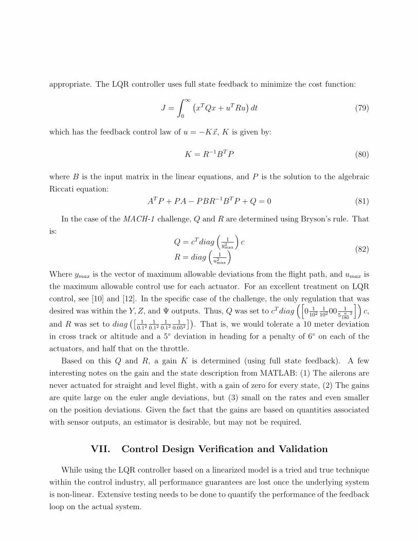
appropriate. The LQR controller uses full state feedback to minimize the cost function:

J =

∫ ∞0

(xTQx+ uTRu

)dt (79)

which has the feedback control law of u = −K~x, K is given by:

K = R−1BTP (80)

where B is the input matrix in the linear equations, and P is the solution to the algebraic

Riccati equation:

ATP + PA− PBR−1BTP +Q = 0 (81)

In the case of the MACH-1 challenge, Q and R are determined using Bryson’s rule. That

is:

Q = cTdiag(

1y2max

)c

R = diag(

1u2max

) (82)

Where ymax is the vector of maximum allowable deviations from the flight path, and umax is

the maximum allowable control use for each actuator. For an excellent treatment on LQR

control, see [10] and [12]. In the specific case of the challenge, the only regulation that was

desired was within the Y, Z, and Ψ outputs. Thus, Q was set to cTdiag([

0 1102

1102 00 1

5 π180

2

])c,

and R was set to diag([

10.12

10.12

10.12

10.052

]). That is, we would tolerate a 10 meter deviation

in cross track or altitude and a 5◦ deviation in heading for a penalty of 6◦ on each of the

actuators, and half that on the throttle.

Based on this Q and R, a gain K is determined (using full state feedback). A few

interesting notes on the gain and the state description from MATLAB: (1) The ailerons are

never actuated for straight and level flight, with a gain of zero for every state, (2) The gains

are quite large on the euler angle deviations, but (3) small on the rates and even smaller

on the position deviations. Given the fact that the gains are based on quantities associated

with sensor outputs, an estimator is desirable, but may not be required.

VII. Control Design Verification and Validation

While using the LQR controller based on a linearized model is a tried and true technique

within the control industry, all performance guarantees are lost once the underlying system

is non-linear. Extensive testing needs to be done to quantify the performance of the feedback

loop on the actual system.

The first stage of verification and validation is to validate the feedback loop on the

linearized system of of which it was designed. This should demonstrate that the ideal per-

formance is good enough to meet the specifications determined in Section V. Excessive

overshoot, or other poorly behaved modes should be addressed at this point until a satisfac-

tory closed loop response has been achieved. Closed loop eigenvalues can be inspected, and

linear simulations used to visualize the performance.

The second stage of verification and validation consists of placing the feedback control

system on the full 6DoF non-linear simulation, and determining if the actual performance is

near that of the linear system performance. Unfortunately, simulation and iteration are the

best tools here to tweak the design until a satisfactory solution can be found.

In the case where the system in linearized about several altitude and Mach number

points, each point has a controller designed and validated for that flight regime, and a gain

scheduling is used to switch between the different controllers.

Unfortunately, our team was not able to complete the control system design successfully,

and thus have not had the chance to validate it on our model. Our attempts at using the

LQR controller did not result in a stabilized trajectory. While more time and iterations

would have been beneficial, there may very well be a flaw in our approach that we were not

able to discover.

VIII. Conclusion

We have presented our methodology for the MACH-1 challenge. We used the supplied

specifications to design a complete 6 degree of freedom simulation of the Mars flyer, complete

with Martian atmosphere and gravity. We used SIMULINK to construct the simulation, and

validated the model both at the individual block level as well as the system level.

Using this model, we found a trim point within the specified trajectory bounds, and

linearized the model at that trim condition. We attempted to design an LQR control based

out output regulation, but could not get the closed loop system to perform well (or even

stabilize).

As a team, we learned many lessons through this contest:

• How to implement a complex Simulink model

Our team had little prior experience setting a complex Simulink model. This project

gave team members experience with implementation details such as setting up lookup

tables and using built-in Simulink blocks from the aerospace blockset such as the 6-

DOF Euler Angle block, and the Aerodynamic Forces and Moments block.

• A flight mechanics background would be beneficial

Our team’s background is focused in computer engineering and feedback control. We

found at times it would be helpful to have intuition, resulting from a flight mechanics

background, about model behavior during simulation. For example, we believe that

the instability of our model is the result of an error, but we have not been able to

identify its source.

• More time

More time, as always would be helpful. The errors that were hardest to find were

signal dimension mismatches which, once identified could easily be rectified using the

Reshape block. We found that we can find a trim point if we eliminated actuator and

sensor error blocks.

In the end, we failed at the task of designing a C-code autopilot routine that could be

handed to the judges, and even failed to find a stabilizing controller. However, the contest

was always more about process than about results, and to that end we feel we have learned

a great deal and have a very healthy respect for the flight control engineers working on the

Mars flyer.

Acknowledgements

This contest was quite a stretch for our group, and there were many helpful individuals

along the way which contributed in ways large and small. Specifically, we would like to

acknowledge the help of Matt Jardin, who in addition to putting this contest together, spent

many hours answering our questions and helping us with the inevitable pitfalls along the

way. Additionally, we would like to acknowledge Sheldon Logan, a fellow student at UCSC

who was originally part of the team, helped with the coefficient modeling, but in the end

withdrew from the project.

Appendix : CFI Data

Mass Properties

minit = 100 [kg] (83)

Iinit =

270 0 0

0 190 0

0 0 460

[kg ·m2] (84)

FSref = 1.2669 [m] (85)

FS = 1.2650 [m] (86)

BLref = 0 [m] (87)

BL = 0 [m] (88)

WLref = 0.3131 [m] (89)

WL = 0.2504 [m] (90)

Engine Model

Tthrust = 5 [s−1] (91)

Kthrust = 250 [N ] (92)

Athrust =

1 0 0

0 0 0

0 0 0

(93)

lthrust =[0 0 0

]T[m] (94)

Veffex = 450000 (95)

Error Model for x and y

ANP = 0.001× 0.376× 9.81 [m2/s4] (96)

XNP = 0.5 [m2] (97)

V NP = 0.5 [m2/s2] (98)

A =

0.99 0.0184 −0.0002 −0.001596

−0.002555 0.9992 −0.02 −0.000845

0.0001986 8.353× 10−5 0.9998 8.353× 10−5

0.0009716 −0.002436 0 0.9974

(99)

B =

0.0002 0.01 0.001596

0.02 0.002555 0.000845

0 −0.0001986 −8.353× 10−5

0 −0.0009716 0.002436

(100)

C =

0.99 −0.001579 0 −0.001579

−0.002551 0.9992 0 −0.0008433

0.0009718 −0.002437 0 0.9976

(101)

D =

0 0.009951 0.001579

0 0.002551 0.0008433

0 −0.0009718 0.002437

(102)

Error Model for z

ANP = 0.001× 0.376× 9.81 [m2/s4] (103)

ZNP = 0.5 [m2] (104)

V NP = 0.5 [m2/s2] (105)

ALTNP = 0.5 [m2] (106)

A =

0.9883 0.01885 −0.0002 −0.001154

−0.003472 0.9993 −0.02 −0.0007021

0.0002889 7.209× 10−5 0.9998 7.209× 10−5

0.001187 −0.002488 0 0.9973

(107)

B =

0.0002 0.005849 0.001154 0.005849

0.02 0.001736 0.0007021 0.001736

0 −0.0001444 −7.209× 10−5 −0.0001444

0 −0.0005933 0.002488 −0.0005933

(108)

C =

0.9884 −0.00114 0 −0.00114

−0.003466 0.9993 0 −0.0007007

0.001187 −0.002489 0 0.9975

(109)

D =

0 0.005815 0.00114 0.005815

0 0.001733 0.0007007 0.001733

0 −0.0005934 0.002489 −0.0005934

(110)

Error Model for Angular States

RATENP = 0.0625(π/180)2 [rad2/s2] (111)

ANGNP = 0.16(π/180)2 [rad2/s2] (112)

A =

0.9852 −0.02

0.001611 0.9998

(113)

B =

0.02 0.01479

0 −0.001611

(114)

C =[0.9852 0

](115)

D =[−0 0.01476

](116)

References

1Doyle, J., “Guaranteed margins for LQG regulators”, IEEE Transactions on Automatic Control , 23(4),1978, pp. 756–757.

2McCormick, B., Aerodynamics, Aeronautics, and Flight Mechanics, John Wiley and Sons, New York,NY, 1979.

3McGeer, T., Kroo, I., “A Fundamental Comparison of Canard and Conventional Configurations,”Journal of Aircraft , Nov. 1983

4Shevell, R. S., Fundamentals of Flight , Prentice-Hall, Inc., Englewood Cliffs, NJ, 1983.5Braun, R. D., Wright, H. S., et al, The Mars Airplane: A Credible Science Platform, IEEE 04-1260,

IEEE Aerospace Conference, Big Sky Montana, March 2004.6Guynn, Mark; Croom, Mark; Smith, Stephen; Parks, Robert; Gelhausen, Paul, Evolution of a Mars

Airplane Concept for the ARES Mars Scout Mission, 2nd AIAA ”Unmanned Unlimited” Systems, Tech-nologies, and Operations - Aerospace, Land, and Sea Conference, Workshop and Exhibition; San Diego, CA;Sep. 15-18, 2003.

7A Concept Study for a Remotely Piloted Vehicle for Mars Exploration: Final Report NASA CR-157942,1978.

8Stephen C. Smith, Andrew S. Hahn, Wayne R. Johnson, David J. Kinney, Julie A. Pollitt, and JamesJ. Reuther, The design of the Canyon Flyer, an airplane for Mars exploration, AIAA-2000-514, AerospaceSciences Meeting and Exhibit, 38th, Reno, NV, Jan. 10-13, 2000.

9Seidelmann, P. K., et al,. 2002. Report of the IAU/IAG working group on cartographic coordinatesand rotational elements of the planets and satellites: 2000. Celest. Mech. Dyn. Astron., 82, pp. 82-110.

10Stengel, R. F., 1994. Optimal Control and Estimation. Dover, New York, New York, pp. 299 – 419.11Stevens, B. L., and Lewis, F. L. Aircraft Control and Simulation. John Wiley & Sons, Inc. New York,

NY. 1992.12Bryson, A., and Y. Ho, Applied Optimal Control , New York: Hemisphere, 1975.