Control System Engg. EE-304-F
63
Control System Engg. EE-304-F
Transcript of Control System Engg. EE-304-F

Control System Engg. EE-304-F

TABLE OF CONTENTS
• Syllabus
• Section-C and D

SYLLABUS
• TIME DOMAIN ANALYSIS :Typical test signals, time response of first order systems to various standard inputs, time response of 2nd order system to step input, relationship between location of roots of characteristics equation, w and wn, time domain specifications of a general and an under-damped 2nd order system, steady state error and error constants, dominant closed loop poles, concept of stability, pole zero configuration and stability, necessary and sufficient conditions for stability Hurwitz stability criterion Routh stability criterion and relative stability. Root locus concept, development of root loci for various systems, stability considerations.

Section-D
• FREQUENCY DOMAIN ANALYSIS , COMPENSATION & CONTROL COMPONENT :Relationship between frequency response and time-response for 2nd order system, polar, Nyquist, Bode plots, stability, Gain-margin and Phase Margin, relative stability, frequency response specifications. Necessity of compensation, compensation networks, application of lag and lead compensation, basic modes of feedback control, proportional, integral and derivative controllers, illustrative examples. Synchros, AC and DC techo-generators, servomotors, stepper motors, & their applications, magnetic amplifier.

Section-C &D
Stability and its different types
i. Root Locus
ii. Polar Plot
iii. Nyquist Plot
iv. Bode Plot
v. Compensators

Stability of a closed loop system
Definition of stability of linear system:
Energised the closed-loop system input a short impulse which move the system from it’s steady-state position and wait. When the transient response has died and the system remove the original position or remain inside a predicted defined small area of the original position the system is stable and linear.
Definition of stability of non-linear system:
Energised the closed-loop system input a short impulse which move the system from it’s steady-state position and wait. If the system remove and remain inside a predicted defined small area of the original position the system is stable.
If the transient response hasn’t died the system is unstable.
)(sGc ( )PFG s)s(G)s(G1
)s(G)s(G)s(W
)s(r
)s(y
PFC
PFCyr

Stability examination from closed loop transfer function
)(sGC )(sGPF
nm
m
m
mn
n
ndt
trdb
dt
tdrbtrbtya
dt
tdya
dt
tyda
)()()()(
)()(1001
01
1
1
01
1
1
)()(
)(
)(
)(1
)(
)(
)()(
)(
asasasa
bsbsbsb
sNsD
sN
sD
sN
sD
sN
sWsr
syn
n
n
n
m
m
m
myr
r(s) y(s)
Unit feedback model
)(
)()()()(0
sD
sNsGsGsG PFC
)()()()(
)()()()(
01
1
1
01
1
1
srbssrbsrsbsrsb
syassyasysasysa
m
m
m
m
n
nm
n
n

Continuation of stability examination from closed loop
)(sGc)(sGp
n
i
i
m
j
jm
ps
zsb
1
1
)(
)(
n
i
t
icTransientieKtx
1
)(
The transient solution is given bz the roots of
the differential equation’s characteristic equation.
001
1
1
aaa n
n
n
The roots are equal the denominator of closed loop transfer function and so it gives transient solution too.
001
1
1
asasas n
n
n

Definition of stability in frequency domain
)(sGc)(sGp
The system is stable if the all real part of the roots of denominator of the transfer function is negative.
0)()(1 sGsG pc
n
1i
i
m
1j
jm
)ps(
)zs(b
)s(r
)s(y
The pi are named the poles and zj are named the zeros

Root Locus

Construction of root loci Step-1: The first step in constructing a root-locus plot is to locate the open-loop poles and zeros in s-plane.
)2)(1()()(
sss
KsHsG
-5 -4 -3 -2 -1 0 1 2-1
-0.5
0
0.5
1
Pole-Zero Map
Real Axis
Imagin
ary
Axis
)2()1( is angle The sss

-5 -4 -3 -2 -1 0 1 2-1
-0.5
0
0.5
1
Pole-Zero Map
Real Axis
Imagin
ary
Axis
Construction of root loci Step-2: Determine the root loci on the real axis.
p1
To determine the root loci on real axis we select some test points. e.g: p1 (on positive real axis).
The angle condition is not satisfied.
Hence, there is no root locus on the positive real axis.

-5 -4 -3 -2 -1 0 1 2-1
-0.5
0
0.5
1
Pole-Zero Map
Real Axis
Imagin
ary
Axis
Construction of root loci Step-2: Determine the root loci on the real axis.
p2
Next, select a test point on the negative real axis between 0 and –1.
Then
Thus
The angle condition is satisfied. Therefore, the portion of the negative real axis between 0 and –1 forms a portion of the root locus.

-5 -4 -3 -2 -1 0 1 2-1
-0.5
0
0.5
1
Pole-Zero Map
Real Axis
Imagin
ary
Axis
Construction of root loci Step-2: Determine the root loci on the real axis.
p4
Similarly, test point on the negative real axis between -2 and – ∞ satisfies the angle condition.
Therefore, the negative real axis between -2 and – ∞ is part of the root locus.

-5 -4 -3 -2 -1 0 1 2-1
-0.5
0
0.5
1
Pole-Zero Map
Real Axis
Imag
inar
y A
xis
Construction of root loci Step-2: Determine the root loci on the real axis.

Construction of root loci Step-3: Determine the asymptotes of the root loci. That is, the root loci when s is far away from origin.
Asymptote is the straight line approximation of a curve
Actual Curve Asymptotic Approximation

Construction of root loci
Step-3: Determine the asymptotes of the root loci.
where
n-----> number of poles
m-----> number of zeros
For this Transfer Function
mn
kasymptotesofAngle
)12(180
)2)(1()()(
sss
KsHsG
03
)12(180
k

Construction of root loci
Step-3: Determine the asymptotes of the root loci.
Since the angle repeats itself as k is varied, the distinct angles for the asymptotes are determined as 60°, –60°, and 180°.
3 when 420
2 when 300
1 when 180
0n whe60
k
k
k
k03
)12(180
k

Construction of root loci
Step-3: Determine the asymptotes of the root loci.
Before we can draw these asymptotes in the complex plane, we need to find the point where they intersect the real axis.
Point of intersection of asymptotes on real axis (or centroid of asymptotes) is
mn
zerospoles

Construction of root loci
Step-3: Determine the asymptotes of the root loci.
For
03
0)210(
)2)(1()()(
sss
KsHsG
13
3

Construction of root loci
Step-3: Determine the asymptotes of the root loci.
-5 -4 -3 -2 -1 0 1 2-1
-0.5
0
0.5
1
Pole-Zero Map
Real Axis
Imagin
ary
Axis
60
60
180
180 , 60, 60
1
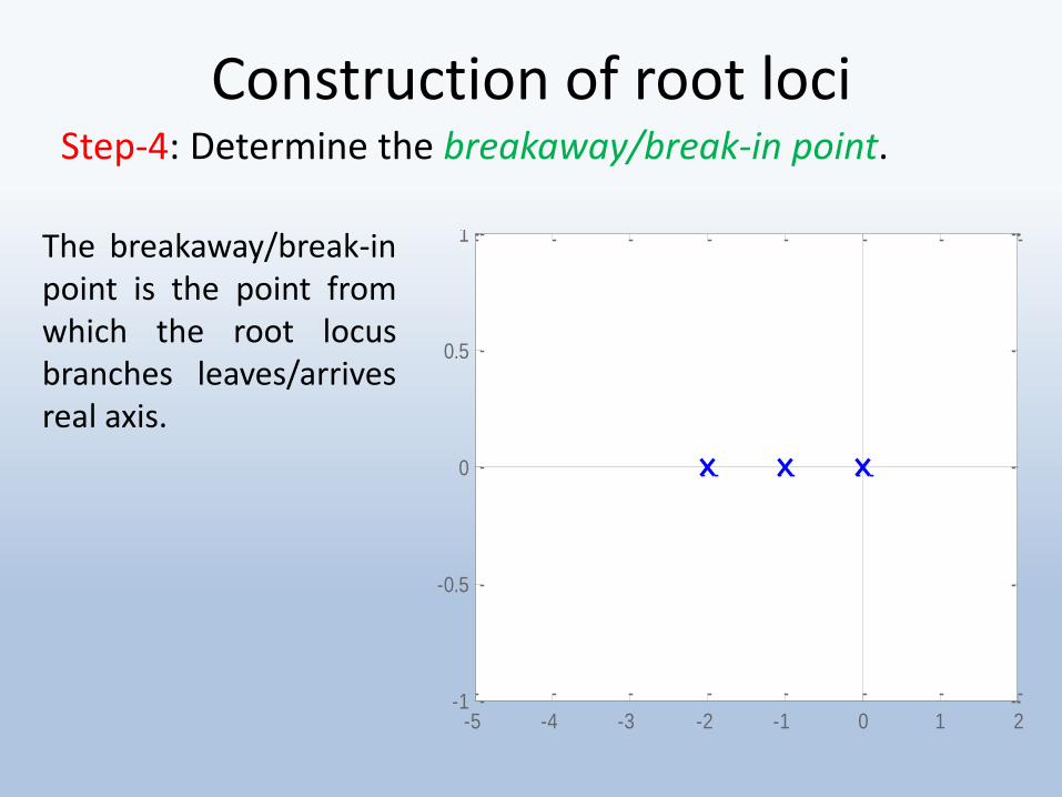
Construction of root loci Step-4: Determine the breakaway/break-in point.
The breakaway/break-in point is the point from which the root locus branches leaves/arrives real axis.
-5 -4 -3 -2 -1 0 1 2-1
-0.5
0
0.5
1
Pole-Zero Map
Real Axis
Imagin
ary
Axis
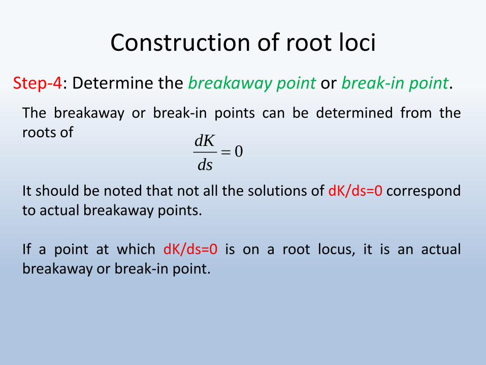
Construction of root loci
Step-4: Determine the breakaway point or break-in point.
The breakaway or break-in points can be determined from the roots of
It should be noted that not all the solutions of dK/ds=0 correspond to actual breakaway points.
If a point at which dK/ds=0 is on a root locus, it is an actual breakaway or break-in point.
0ds
dK

Construction of root loci
Step-4: Determine the breakaway point or break-in point.
Set dK/ds=0 in order to determine breakaway point.
)2)(1( sssds
d
ds
dK
sssds
d
ds
dK23 23
263 2 ssds
dK
0263 2 ss
0263 2 ss
5774.1
4226.0
s

Construction of root loci
Step-4: Determine the breakaway point or break-in point.
Since the breakaway point needs to be on a root locus between 0 and –1, it is clear that s=–0.4226 corresponds to the actual breakaway point.
Point s=–1.5774 is not on the root locus. Hence, this point is not an actual breakaway or break-in point.
5774.1
4226.0
s
)2)(1()()(
sss
KsHsG

Construction of root loci
Step-4: Determine the breakaway point.
-5 -4 -3 -2 -1 0 1 2-1
-0.5
0
0.5
1
Pole-Zero Map
Real Axis
Imagin
ary
Axis
60
60
1804226.0s

Construction of root loci Step-5: Determine the points where root loci cross the imaginary axis.
Let s=jω in the characteristic equation, equate both the real
part and the imaginary part to zero, and then solve for ω and K.
For present system the characteristic equation is
023 23 Ksss
02)(3)( 23 Kjjj
0)2()3( 32 jK

Construction of root loci Step-5: Determine the points where root loci cross the imaginary axis.
Equating both real and imaginary parts of this equation to zero
Which yields
0)2()3( 32 jK
0)3( 2 K
0)2( 3


-7 -6 -5 -4 -3 -2 -1 0 1 2-5
-4
-3
-2
-1
0
1
2
3
4
5
Root Locus
Real Axis
Imagin
ary
Axis

Polar Plot & Nyquist Plot

Nyquist stability criteria
Topics to be covered include:
• Nyquist stability criteria.
• Minimum phase systems.
• Simplified Nyquist stability criterion.

33
( )kf s
Nyquist path Nyquist plot
0111 kNPZ
000 NPZ
Nyquist fundamental
0111 kNPZ

Example: Discuss about the RHP roots of following system.
)1(
)1(2)(
ss
ssf
1800
22)(
ssf
22545
22)(
ssf
27090
22)(
ssf
9090
22)(
ssf
4545
22)(
ssf
00
22)(
ssf
Ver
y im
po
rtan
t p
art
?
0)1(
)1(21
ss
sk

Example: Discuss about the RHP roots of the system.
0)1(
)1(21
ss
sk
)1(
)1(2)(
ss
ssf
)1(
)1(2)(
jj
jjf
)( jf
?
?
Which point is very important?
dennumjf )( )tan90(tan180 11 1tan290
10)( jf02
)1(
)11(2)1(
jj
jjf
1
2
1
2
0Im(f)let ly equivalentOr

Example: Discuss about the RHP roots of the following system for different values of k.
0)1(
)1(21
ss
sk
1
21 1
1110 NPZk 101 Z
Unstable( one RHP root) 11 Z
1110 NPZk 11 NZ
2
0
1Z
05.0 k
5.0k
Stable
Unstable (two RHP root)
More Study:
000 NPZ 101

Bode Plot

Bode plot
• 1st order or higher terms that can be written as a product of 1st order terms
– 4 cases:
• 2nd order terms
– 2 cases:
ss
asas
1,,
)(
1),(
22
22
2
1,2
nn
nnss
ss

)()( assG
)1()()( a
jaajjG
ω = 0
aM
ajG
log20log20
)(
ω >> a
log20log20
90)()(
M
ja
jajG
phase = 0
phase = 90
ω = a
3log202log20log20
)()(
aaM
ajajG phase = 45
First order terms Case I: one zero at -a

Asymptotes (approximation)
Break frequency
= freq. at which mag. has changed by 3 db
12 10

3 dB at break frequency

)(
1)(
assG
)1(
1
)(
1)(
a
ja
ajjG
ω = 0
)/1log(20log20
/1)(
aM
ajG
ω >> a
log20log20
9011
)(
1)(
M
j
aja
jG
phase = 0
phase = -90
ω = a 3)/1log(20)2/1log(20log20 aaM
phase = -45
First order terms Case II: one pole at -a

G(s) = s
G(s) = 1/s
G(s) = s+a
G(s) = 1/(s+a)

Bode Plots Find magnitude and phase of each term
and sum them up!!!
)()()()()(
)(log20)(log20log20
)(log20)(log20log20)(log20
)()(
)()()(
))((
))(()(
2121
21
21
21
21
21
21
pspsszszsKsG
pspss
zszsKsG
pspss
zszsKsG
pspss
zszsKsG
m
m
m
m
mag(num)-mag(den)
phase(num)-phase(den)

Example
sketch bode plot of
)2)(1(
)3()(
sss
ssG
break frequency at 1,2,3

Frequency small 1 2 3
s -20 -20 -20 -20
1/(s+1) 0 -20 -20 -20
1/(s+2) 0 0 -20 -20
(s+3) 0 0 0 20
Total Slope -20 -40 -60 -40
Slope at each break frequency for magnitude plot

Magnitude Plot

Frequency small 0.1 0.2 0.3 10 20 30
s 0 0 0 0 0 0 0
1/(s+1) 0 -45 -45 -45 0 0 0
1/(s+2) 0 0 -45 -45 -45 0 0
(s+3) 0 0 0 45 45 45 0
Total Slope 0 -45 -90 -45 0 45 0
Slope at each point for phase plot

Phase Plot

Stability examination from transfer function of opened-loop
)(sGc)(sGp
)s(G)s(G)s(G 0pc
Opened-loop transfer function
01)(0)(1 jjGsG olol From definition of stability: 180j)(j
0 e1e)(A0j1)j(G
Gain cross over Frequeny:The frequency at which the open-loop system gain is unity is termedthe gain-crossover frequency. Phase cross over Frequeny:The frequency at which the open-loop system phase-shift is -180° is termed the phase-crossover frequency. Note: The system is stable if plots of the opened-loop transfer function at the gain-crossover frequency the phase-shift less than -180° and at the phase-crossover frequency the amplitude gain less than unity.

Gain margin and phase margin
Opened-loop transfer function: )()(01)( j
ol eAjjG
The gain margin is the reciprocal of open-loop gain at the phase-crossover frequency. Expressed in decibel the gain margins is: -20log(open-loop’s gain at the phase-crossover frequency) dB The phase margin is the difference of the phase-shift of the system and -180° at the gain-crossover frequency. Note: The system is stable if plots of the opened-loop transfer function at the gain-crossover frequency has a positive the phase margin and at the phase-crossover frequency has a positive the gain margin.

Stability examination from transfer function of opened-loop
)(j
0 e)(A0j1)j(G
Plots on j (s) plane is named Nyquist diagram. This is a point on the s plane. If the area of the s plane which is bordered by the positive real axis and the Nyquist plots doesn’t cover this point than the system is stable.
Independent plots the amplitude gain and phase-shift on lg axis is named Bode diagram. It is the x axis line on the amplitude plots and the -180 phase-shift line on the phase-shift plots. If the gain and phase margin criterion is true the system is stable.

Advantages of working with Bode plots
n
1i
i
m
1j
j
i0
)sT1(
)s1(
s
K)s(G
Bode form of opened-loop transfer function
Bode plots of systems in series simply add. Bode’s important phase-gain relationship is given. A much wider range of system behaviour can be displayed on a single plot. Dynamic compensator design can be based on Bode plots.

State Space Analysis

)()()(
)()()(
tDutCxty
tButAxtxdt
d
State equation
Output equation
Dynamic equation
1
2
1
)(
)(
)(
)(
nn tx
tx
tx
tx
1
2
1
)(
)(
)(
)(
rr tu
tu
tu
tu
1
2
1
)(
)(
)(
)(
pp ty
ty
ty
ty
State space
State variable
r- input p- output
nnA
rnB
npC
rpD
1
2
1
)0(
)0(
)0(
)0(
nnx
x
x
x

Motivation of state space approach
3
1
)(
)(
s
s
sU
sY
+ -
)(tu )(ty
)1(
1
s
s
1
2
s +
)(tn noise
)3)(1(
)1(2
)(
)(0
ss
s
sN
sEu
BIBO stable
unstable
Transfer function
Example 1 )(te

1
1
s
s
1
1
s
)(tu )(ty
1
1
su
yBIBO stable, pole-zero cancellation
-2 s
1
s
1
)(tu )(ty
+ +
+
+ +
-
1x 2x1x 2x)(tv
us
uv
ss
s
u
v
1
2
1
21
1
1

2
212
11 2
xy
uxxx
uxx
202
101
)0(
)0(
xx
xx
)(2
1)
2
1()()(
)(2)(
1010202
101
tuexeexxtxty
tuexetx
ttt
tt
2010
2010
2.2
0.1
xxif
xxif
then system stable
State-space description Internal behavior description
)]()[()0(])[()( 1111 sBUAsILxAsILtx

Example
M2 M1
B3 B1 B2
K 1y2y
)(tf
0)()(
)()()(
121222322
212121111
yyKyyByByM
tfyyKyyByByM
23
12
211
yx
yx
yyx
let
)(
0
10
)(
)(110
1
3
2
1
2
32
2
2
2
1
2
1
21
1
3
2
1
tfM
x
x
x
M
BB
M
B
M
K
M
B
M
BB
M
K
x
x
x

aR aL
ai
tea
fR
fL
teb
m
mJLT
Armature circuit Field circuit
te f
dt
diLeiRte a
abaaa )(
mbb ke
a
a
m
a
ba
a
aa eLL
ki
L
R
dt
di 1
L
m
m
m
m
aim
Tdt
dB
dt
dJ
ikT
2
2
m
m
L
m
m
m
m
a
m
im
dt
d
TJdt
d
J
Bi
J
k
dt
d
1
Example
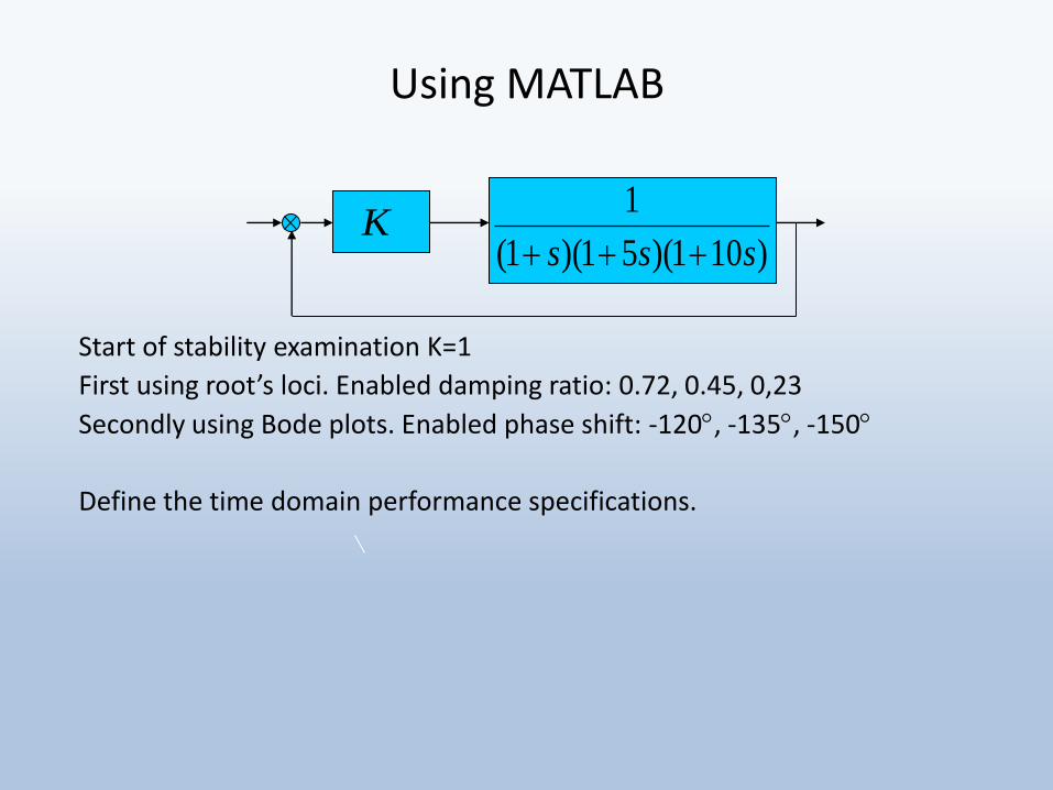
Using MATLAB
Start of stability examination K=1
First using root’s loci. Enabled damping ratio: 0.72, 0.45, 0,23
Secondly using Bode plots. Enabled phase shift: -120, -135, -150
Define the time domain performance specifications.
K)101)(51)(1(
1
sss

Summary questions
• Definition of stability of linear and non-linear systems.
• Which methods have used the closed-loop transfer function to examine the stability a control system?
• Which methods have used the opened-loop transfer function to examine the stability a control system?
• Explain the following terms: phase margin, gain margin.
• Explain what is meant by the term “dead time” in control and how it may affect the stability of a control loop.

NPTEL/other online links
• https://nptel.ac.in/courses/108101037/
• https://www.tutorialspoint.com/control_systems/control_systems_introduction.htm
• https://en.wikibooks.org/wiki/Control_Systems/Introduction
• https://lecturenotes.in/subject/52/control-system-engineering-cse
• https://www.researchgate.net/publication/265168969_Control_Systems_Engineering