Control point adjustment for B-spline curve approximation

Huaiping Yanga,b, Wenping Wanga,*, Jiaguang Sunb

aThe University of Hong Kong, Hong Kong, ChinabTsinghua University, Beijing, China

Abstract

Pottmann et al. propose an iterative optimization scheme for approximating a target curve with a B-spline curve based on square distance

minimization, or SDM. The main advantage of SDM is that it does not need a parameterization of data points on the target curve. Starting

with an initial B-spline curve, this scheme makes an active B-spline curve converge faster towards the target curve and produces a better

approximating B-spline curve than existing methods relying on data point parameterization. However, SDM is sensitive to the initial B-spline

curve due to its local nature of optimization. To address this, we integrate SDM with procedures for automatically adjusting both the number

and locations of the control points of the active spline curve. This leads to a method that is more robust and applicable than SDM used alone.

Furthermore, it is observed that the most time consuming part of SDM is the repeated computation of the foot-point on the target curve of a

sample point on the active B-spline curve. In our implementation, we speed up the foot-point computation by pre-computing the distance

field of the target curve using the Fast Marching Method. Experimental examples are presented to demonstrate the effectiveness of our

method. Problems for further research are discussed.

q 2003 Elsevier Ltd. All rights reserved.

Keywords: B-spline curve; Shape approximation; Optimization; Squared distance

1. Introduction

1.1. B-spline curve fitting problem

The B-spline curve fitting problem is to produce a B-

spline curve to approximate a target curve within a pre-

specified tolerance. We assume that the target curve is

defined in 2D plane by a sequence of ordered dense data

points or a curve given implicitly or explicitly (i.e. by a

parametric equation).

There is much work in the literature on solving the

curve-fitting problem using the B-spline curve. However,

most of the existing methods require a parameterization

of data points on the target curve, and little consideration

has been given to the automatic placement of a minimal

number of control points of an approximating B-spline

curve satisfying a pre-specified error tolerance. It is

beyond the scope of the present paper to give a detailed

review of all the existing work; we will only

review those most relevant results. The reader may

consult [6] for a general introduction to the curve-fitting

problem.

1.2. Methods based on data parameterization

A parameterization of target data points is often needed

for B-spline curve approximation [4,6]. Let Pk; k ¼

1; 2;…;N; denote a sequence of ordered data points on a

target curve G: Let XðuÞ ¼Pn

i¼1 BiðuÞDi denote a B-spline

curve to be determined to approximate the target curve G;

where BiðuÞ are the B-spline basis functions of a certain

order and Di are control points. Suppose that, through some

method [17], the data points Pk are made to correspond to

the parameter values uk in the domain of the curve XðuÞ:

Then the usual approach to determining the control points

Di is based on a least squares formulation and computes the

minimizer of an objective function

F ¼X

k

kXðukÞ2 Pkk2þ lFs; ð1Þ

where Fs; called the regularization term, is quadratic in the

control points Di and is used to enforce the fairness of the

final approximating curve [1,2,8,23]. Therefore, the mini-

mizer of F can be found by solving a system of linear

equations.

Assigning parameter values to data points, a procedure to

be referred to as data parameterization, is unnatural for

measuring the geometric difference between a target curve

0010-4485/$ - see front matter q 2003 Elsevier Ltd. All rights reserved.

doi:10.1016/S0010-4485(03)00140-4

Computer-Aided Design 36 (2004) 639–652

www.elsevier.com/locate/cad

* Corresponding author.

E-mail address: wenping@csis.hk.hku (W. Wang).

and its approximating B-spline curve; a suitable measure-

ment of the difference between two curves should be defined

by a distance between two point sets, such as the Hausdorff

distance [7]. Different ways of data parameterization lead to

different approximation results. Fundamentally, the notion

of the optimal data parameterization is theoretically elusive

and computationally difficult to achieve. An improper

data parameterization may considerably compromise the

quality and efficiency of approximation. The following

three methods for data parameterization have been proposed

[15,23,24]: uniform parameterization, chord-length

parameterization, and centripetal parameterization.

Some recent research aims at correcting assigned

parameter values iteratively to improve the approximation

error [5,11–13,19]. Such correction procedures are rather

time-consuming, typically taking 100–300 iterations to

converge [12].

1.3. Squared distance minimization

Pottmann et al. [17] propose an optimization scheme for

B-spline curve approximation that does not require data

parameterization. Starting with an initial B-spline curve,

this method attempts to make an active B-spline curve

converge towards the target curve by minimizing an

objective function defined by local approximate squared

distances of the target curve. For brevity, this scheme will

be referred to as squared distance minimization, or SDM.

The main idea of SDM is as follows. For each iteration,

one computes the foot-points Ok on the target curve of a

number of sample points Xk on the active B-spline curve.

Here, we treat the Xk as variable points expressed as linear

combinations of the control points Di: (The number of

sample points per piece of the B-spline curve is a user-

specified parameter; we normally use 10 sample points on

each piece of a cubic B-spline curve.) Let X0k denote

the current location of the point Xk: Then the local

approximate squared distance of the point Xk to the target

curve is given by

Fþd ðXkÞ ¼

d

d þ lrlx2

1 þ x22; ð2Þ

where x1 and x2 are the coordinates of Xk with respect to the

Frenet frame of the target curve at the foot-point Ok; d ¼

kX0k 2 Okk; and r is the curvature radius of the target curve at

Ok: (See Fig. 1. The reader is referred to Ref. [18] for a

detailed derivation and discussion of this formula.) Then the

control points Di of an approximating B-spline curve are

computed by minimizing the objective function

F ¼X

k

Fþd ðXkÞ þ lFs; ð3Þ

which is quadratic in the Di; and thus can be solved using the

quasi-Newton method.

SDM converges very fast. Our tests show that, with an

appropriately specified initial B-spline curve, no more than

20 iterations are needed for the convergence of SDM in

most cases. Furthermore, due to its independence of data

parameterization, SDM produces better approximating B-

spline curves than those methods relying on data para-

meterization, since SDM makes the sample points on the

active B-spline curve move towards the target curve, rather

than simply towards their corresponding foot-points.

However, because SDM is based on local optimization,

its approximation results can be very sensitive to the initial

B-spline curve. We explain this problem by the example in

Fig. 2, where the target curve is shown as the dotted curve

and the initial B-spline curve as the solid curve. With the

initial control points shown in Fig. 2(a), SDM produces

the approximating curve in Fig. 2(b), in which there are

redundant control points on the right part of the B-spline

curve, but too few control points on the left part to allow an

acceptable approximation error. In contrast, if a different

Fig. 1. The local squared distance used in SDM.

Fig. 2. Effects of different initial B-spline curves. (a) An initial order-3 B-

spline curve; (b) Unsatisfactory approximation generated by SDM from the

control points in (a); (c) An initial B-spline curve different from that in (a);

(d) Better approximation generated by SDM from the control points in (c).

H. Yang et al. / Computer-Aided Design 36 (2004) 639–652640

initial B-spline curve with the same number of control

points as shown in Fig. 2(c) is used, SDM produces the

approximating curve in Fig. 2(d), which is clearly more

acceptable than the approximating curve in Fig. 2(b).

Another example is shown in Fig. 3. Here, by applying

SDM alone, the two different but similar initial B-spline

curves (Fig. 3(a) and (c)) lead to two radically different

approximation results (Fig. 3(b) and (d)). These examples

show clearly the importance of specifying an appropriate

initial B-spline curve or providing an automatic mechanism

of adjusting the control points of an active B-spline curve on-

the-fly in order to obtain a satisfactory approximating curve.

This provides the motivation for our work on integrating

SDM with procedures for control point adjustment.

1.4. Outline of our method

In practice, it is extremely difficult, if not impossible, to

specify an initial B-spline curve a priori with a suitable

number of control points distributed appropriately so as to

yield a satisfactory approximating curve. Therefore, we

present a new method for adjusting the control points of the

active B-spline curve. Our goal is, through the addition of

new control points or the removal of redundant control

points, to generate a B-spline curve with as few control

points as possible that approximates a given target curve to

within a pre-specified error tolerance.

More specifically, given a target curve and an initial B-

spline curve, which is normally specified by the user, we first

use SDM of Pottmann et al. to update the initial B-spline

curve to get a B-spline curve C approximating the target

curve. Then the approximation error of each segment of the

B-spline curve C is evaluated. If a segment of the curve C has

a large error, then this can be attributed to that the segment

does not have enough control points. Therefore, we insert

new control points one by one to this segment till the

approximation error of the segment is reduced to within the

error tolerance. On the other hand, if we detect that a segment

of the curve C has redundant control points, we remove the

control points of the segment one by one till the control points

cannot be removed anymore without making the error larger

than the error tolerance. Once the control points have been

adjusted as above, SDM is applied again to produce a new

approximating B-spline curve. This procedure is repeated

until a satisfactory result is obtained. Fig. 4 shows an example

using this method.

In addition, we observe that the most time-consuming part

of SDM is the repeated computation of the foot-point on the

target curve of a sample point on the active B-spline curve. In

our method we speed up this computation by pre-computing

the discrete distance field of the target curve using the Fast

Marching Method [22], which is originally proposed in the

framework of the level-set method. This improvement of

efficiency makes our method more applicable in practice.

The rest of this paper is organized as follows. In Section 2

we discuss our strategy of adjusting the control points,

Fig. 3. Two different initial B-spline curves of order-3 with eight control

points in (a) and (c) are used to approximate the target curve defined by

x20 þ y20 ¼ 1: The initial control points in (a) and (c) are evenly distributed

on a circle, and differ only in orientation. Their corresponding final

approximating B-spline curves generated by SDM are shown in (b) and (d),

respectively.

Fig. 4. Adjusting the distribution of control points. (a) Initial control points

of an order-4 B-spline curve (solid) and a target curve (dashed); (b) The

approximation result by SDM; (c) The approximation result after control

point adjustment; (d) The final result after further adjustment. The thick

dashed lines denote the part containing redundant control points and the

thick black lines denote the B-spline piece with a large local error, i.e.

where control point insertion is needed.

H. Yang et al. / Computer-Aided Design 36 (2004) 639–652 641

i.e. the insertion of a new control point and the removal of

redundant control points. In Section 3, we give an outline of

our complete algorithm for B-spline curve approximation

and discuss the specification of an initial B-spline curve.

In Section 4, we discuss how to use the pre-computed

distance field of a target curve to speed up the foot-point

computation. We present experimental results in Section 5

and conclude the paper in Section 6 with discussions and

problems for further research.

2. Adjustment of control points

In this section we discuss how to adjust the control points

of an active B-spline curve using SDM so as to obtain a B-

spline curve that approximates a given target curve to within

a pre-specified error tolerance e0 and has as few control

points as possible. There are two parts in this adjustment

strategy:

† Select and remove locally redundant control points;

† Insert new control points to a segment of the active B-

spline curve whose approximation error is large and

cannot be further reduced by optimization due to the lack

of degree of freedom.

We assume that the knot sequence of the B-spline curve

is fixed and is independent of the shape of the target curve.

Uniform or uniform-periodic B-spline curves are used in all

examples presented in this paper.

2.1. Removal of redundant control points

Each piece of a K-th order B-spline curve is dependent

on K consecutive control points [16]. Suppose that an active

B-spline curve C has n control points. Let Ej be the current

approximation error of the j-th piece Lj of the piecewise B-

spline curve C: Then Ej is defined by

Ej ¼1

m

Xm

i¼1

di; ð4Þ

where m is the number of sample points Xi on Lj and di is the

distance between Xi and its foot-point Oi on the target

curve G: The approximation error of the whole curve C is

defined by

E ¼1

NL

XNL

j¼1

Ej; ð5Þ

where NL is the total number of pieces of the B-spline

curve C:

We first consider how to detect a piece of the curve C that

contains redundant control points, and then how to remove

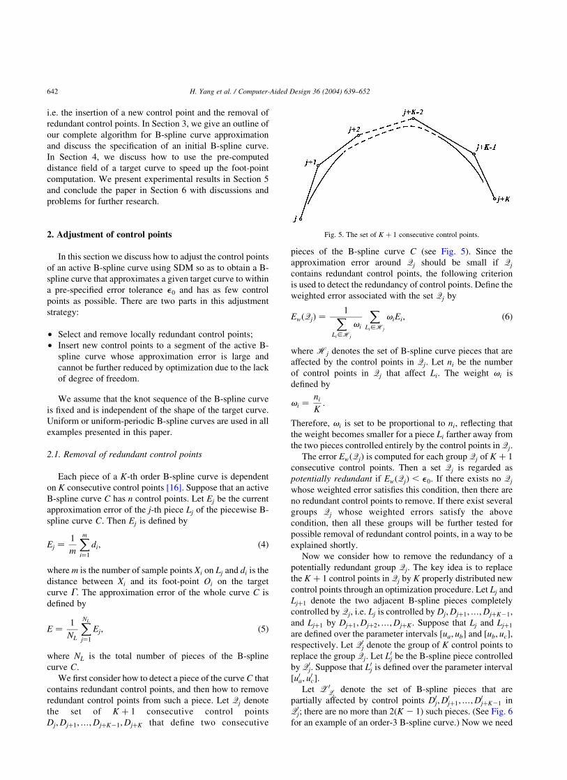
redundant control points from such a piece. Let Qj denote

the set of K þ 1 consecutive control points

Dj;Djþ1;…;DjþK21;DjþK that define two consecutive

pieces of the B-spline curve C (see Fig. 5). Since the

approximation error around Qj should be small if Qj

contains redundant control points, the following criterion

is used to detect the redundancy of control points. Define the

weighted error associated with the set Qj by

EwðQjÞ ¼1X

Li[Hj

vi

X

Li[Hj

viEi; ð6Þ

where Hj denotes the set of B-spline curve pieces that are

affected by the control points in Qj: Let ni be the number

of control points in Qj that affect Li: The weight vi is

defined by

vi ¼ni

K:

Therefore, vi is set to be proportional to ni; reflecting that

the weight becomes smaller for a piece Li farther away from

the two pieces controlled entirely by the control points in Qj:

The error EwðQjÞ is computed for each group Qj of K þ 1

consecutive control points. Then a set Qj is regarded as

potentially redundant if EwðQjÞ , e0: If there exists no Qj

whose weighted error satisfies this condition, then there are

no redundant control points to remove. If there exist several

groups Qj whose weighted errors satisfy the above

condition, then all these groups will be further tested for

possible removal of redundant control points, in a way to be

explained shortly.

Now we consider how to remove the redundancy of a

potentially redundant group Qj: The key idea is to replace

the K þ 1 control points in Qj by K properly distributed new

control points through an optimization procedure. Let Lj and

Ljþ1 denote the two adjacent B-spline pieces completely

controlled by Qj; i.e. Lj is controlled by Dj;Djþ1;…;DjþK21;

and Ljþ1 by Djþ1;Djþ2;…;DjþK : Suppose that Lj and Ljþ1

are defined over the parameter intervals ½ua; ub� and ½ub; uc�;

respectively. Let Q0j denote the group of K control points to

replace the group Qj: Let L0j be the B-spline piece controlled

by Q0j: Suppose that L0

j is defined over the parameter interval

½u0a; u

0c�:

Let Z0Q0

jdenote the set of B-spline pieces that are

partially affected by control points D0j;D

0jþ1;…;D0

jþK21 in

Q0j; there are no more than 2ðK 2 1Þ such pieces. (See Fig. 6

for an example of an order-3 B-spline curve.) Now we need

Fig. 5. The set of K þ 1 consecutive control points.

H. Yang et al. / Computer-Aided Design 36 (2004) 639–652642

to determine the distribution of the K new control points in

Q0j so that the approximation error around Qj is increased as

little as possible. To this end, we adopt the following two

requirements:

1. L0j; i.e. the piece of B-spline curve controlled byQ0

j; should

be close to the target curve. Note that the control points

D0j;D

0jþ1;…;D0

jþK21 in Q0j are unknown at this point and

need to be determined. Suppose 2m points X0ðu0iÞ; i ¼

1; 2;…; 2m; are sampled evenly in the interval ½u0a; u

0c�:

Then we use the following objective function defined by

the approximate local squared distance formula (2) to

measure the closeness between L0j and the target curve:

FL0j¼

X2m

i¼1

FþdiðX0ðu0

iÞÞ; u0i [ ½u0

a; u0c�: ð7Þ

Here, in order to define the distance functions FþdiðX0ðu0

iÞÞ;

we get the corresponding points XðuiÞ ,i ¼ 1; 2;…; 2m; on

Lj and Ljþ1 of X0ðu0iÞ through the following linear mapping

from ½u0a; u

0c� to ½ua; uc�;

ui ¼ ua þuc 2 ua

u0c 2 u0

a

ðu0i 2 u0

aÞ:

Then we use the foot-point Oi of XðuiÞ and the distance

di ¼ kXðuiÞ2 Oik to define FþdiðX0ðu0

iÞÞ (Section 1.3)

(see Fig. 7).

2. The B-spline pieces L0k in Z0

Q0jshould also be close to the

target curve. Their difference is measured by the error

termP

L0k[Z0

Q0j

FL0k: Here, FL0

kmeasures the difference

between L0k and the target curve, defined by the sum of

approximate local squared distances

FL0k¼

Xm

i¼1

FþdiðX0ðu0

iÞÞ; u0i [ ½u0

1;k; u02;k�; ð8Þ

where ½u01;k; u

02;k� is the parameter interval of L0

k; and

X0ðu0iÞ; i ¼ 1; 2;…;m; are the m evenly sampled points on

L0k: Let Lk be the corresponding curve piece of L0

k before

Qj is replaced by Q0j: Suppose that Lk is defined over

½u1;k; u2;k�: Then we get the corresponding points XðuiÞ;

i ¼ 1; 2;…;m of X0ðu0iÞ through the linear mapping

ui ¼ u1;k þu2;k 2 u1;k

u02;k 2 u0

1;k

ðu0i 2 u0

1;kÞ; u0i [ ½u0

1;k; u02;k�:

Then the foot-point Oi of XðuiÞ and di ¼ kXðuiÞ2 Oik are

used to obtain the distance function FþdiðX0ðu0

iÞÞ.

Hence, by combining the two requirements above, the

unknown control points D0j;D

0jþ1;…;D0

jþK21 can be com-

puted as the minimizer of the objective function

FQ ¼ FL0jþ

X

L0k[Z0

Q0j

FL0k; ð9Þ

which is quadratic in D0j;D

0jþ1;…;D0

jþK21:

When there are more than one group of control points Qj

satisfying EwðQjÞ , e0; the minimum value of FQ is

computed for each of these groups, and the group Qj with

the smallest FQ will be considered as the most redundant one

and be replaced by Q0j; while the others are kept unchanged.

Note that the removal of a potentially redundant control

point is confirmed only if the approximation error still meets

the error tolerance after the removal of that control point;

otherwise, the removal will be revoked, i.e. no control point

will be removed.

2.2. Insertion of new control points

When there are too few control points, either locally or

globally, the active B-spline curves may not have enough

Fig. 7. The relationship between X0ðu0iÞ; XðuiÞ and Oi:

Fig. 6. An example of removing a redundant control point from an order-3

B-spline curve. The group Qj is initially composed of four control points

6; 7; 8; 9; and is replaced by Q0j composed of three new control points

60; 70; 90: The B-spline pieces in Z0Q0

jthat are partially affected by Q0

j include

the pieces determined by control point set ð4; 5; 60Þ; ð5; 60; 70Þ; ð70; 90; 10Þ and

ð90; 10; 11Þ; which correspond to ð4; 5; 6Þ; ð5; 6; 7Þ; ð8; 9; 10Þ and ð9; 10; 11Þ;

respectively. The B-spline curve is dashed before the control point removal

and solid after the removal. Note that the shape of the B-spline curve is well

preserved by the removal of a redundant control point.

H. Yang et al. / Computer-Aided Design 36 (2004) 639–652 643

flexibility to approximate a target curve of complex shape.

In this case, new control points need to be inserted. We first

need to determine if any piece of the active B-spline curve

has a large approximation error that cannot be reduced by

optimization, and, if such a piece of curve exists, a new

control point is inserted to that piece. By inserting a control

point, we mean replacing K consecutive control points by

K þ 1 appropriately distributed new control points such that

the approximation error is reduced.

Again, the approximation error Ej of a piece Lj of the

active B-spline curve is given by Eq. (4). We select

the segment Lj0that gives the maximal error among all

the pieces, i.e. Ej0¼ maxj ðEjÞ; and consider adding a

new control point to the piece Lj0: Let

Dj0;Dj0þ1;…;Dj0þK21 be the K control points of Lj0

:

Suppose that the K control points are replaced by K þ 1

new control points D0j0;D0

j0þ1;…;D0j0þK21;D

0j0þK whose

locations are to be determined. Then the B-spline piece

Lj0is replaced by two new pieces L0

j0and L0

j0þ1 which

have the control points D0j0;D0

j0þ1;…;D0j0þK21 and

D0j0þ1;D

0j0þ2;…;D0

j0þK ; respectively, as shown in Fig. 8.

In order to determine the control points

D0j0;D0

j0þ1;…;D0j0þK21;D

0j0þK ; we select the midpoint of Lj0

as a break point Pr to break Lj0into two pieces (Fig. 8(a)).

This is similar to the interval midpoint strategy [4], but with

the major difference that we use the middle point as a break

point, rather than as a new control point in Ref. [4]. Suppose

that Lj0is defined over the parameter interval ½u1;j0

; u2;j0� and

the parametric value of Pr is u0; j0: Then L0

j0and L0

j0þ1 are

defined over ½u01; j0

; u00; j0

� and ½u00; j0

; u02; j0

�; respectively. Let

Z0j0

denote the set of B-spline pieces that are partially

affected by the control points D0j0;D0

j0þ1;…;D0j0þK21;D

0j0þK :

(There are 2ðK 2 1Þ such pieces for a closed B-spline

curve.) Define the following objective function

FO ¼ ðFL0j0

þ FL0j0þ1

Þ þX

L0k[Z0

j0

FL0k; ð10Þ

where FL0j0

is the approximation error between L0j0

and the

target curve, which is given by FL0j0¼

Pmi¼1 Fþ

diðX0ðu0

iÞÞ;

u0i [ ½u0

1; j0; u0

0; j0�; where Fþ

diðX0ðu0

iÞÞ is the local squared

distance between X0ðu0iÞ and the target curve, and di is

the distance between XðuiÞ and Oi: The m points X0ðu0iÞ;

i ¼ 1; 2;…;m; are evenly sampled in the parameter interval

½u01;j0

; u00;j0

� and the point XðuiÞ are determined from X0ðu0iÞ

through the linear mapping from u0i [ ½u0

1; j0; u0

0; j0� to ui [

½u1; j0; u0; j0

�:

The term FL0j0þ1

¼Pm

i¼1 FþdiðX0ðu0

iÞÞ is similarly defined

with the linear mapping from u0i [ ½u0

0; j0; u0

2; j0� to ui [

½u0; j0; u2; j0

�; and the error term FL0k¼

Pmi¼1 Fþ

diðX0ðu0

iÞÞ is

defined in the same way as Eq. (8) for control point removal.

Clearly, the objective function FO (10) is quadratic in the

unknown control points D0j0;D0

j0þ1;…;D0j0þK21;D

0j0þK :

Therefore, these control points can be computed efficiently

by the quasi-Newton optimization. Fig. 9 shows an example

of inserting a new control point to an order-3 B-spline curve.

Some remarks are in order about other existing methods

for inserting new control points [3,4,12]. These methods are

all for B-spline curve approximation based on data point

parameterization.

† Interval midpoint strategy. Dierckx [4] proposes that a

new control point be introduced in the middle of the

piecewise-polynomial curve which has a large approxi-

mation error from the target curve.

† Largest displacement strategy. Lu and Milios [12]

suggest that the new control point be inserted at the

point on the spline which has the maximum displacement

from the target curve.

† PERM strategy. Cham and Cipolla [3] attempt to

estimate the position on the spline to introduce a hinge

Fig. 8. Lj0is replaced by L0

j0and L0

j0þ1 after inserting a new control point.

Fig. 9. An example of control point insertion for an order-3 B-spline curve.

The target curve is shown as the dotted curve. The B-spline curve is dash-

dotted before control point insertion and solid after the insertion. The

control points ð3; 4; 5Þ are replaced by ð30; 40; 400; 50Þ: Clearly, a better

approximation result is achieved by inserting the new control point.

H. Yang et al. / Computer-Aided Design 36 (2004) 639–652644

such that the potential for reducing the approximation

error is maximized. They call it the potential for energy-

reduction maximization (PERM) method.

Cham and Cipolla compare the three methods above [3]

and conclude that the first two methods are prone to be

trapped in a weak local minimum while the PERM method

yields near-optimal results in most cases. All these methods

just add a new control point to the B-spline piece without

redistributing the existing control points.

3. Complete algorithm

3.1. Algorithm

The algorithm takes as input a target curve, an initial B-

spline curve and a user-specified error tolerance e0: It

outputs a B-spline curve approximating the target curve

within the error tolerance e0:

Begin

(1) Compute a discrete distance field of the target

curve on a grid using the Fast Marching Method.

The distance to the target curve, together with

other information, such as the curvature and

normal vector of the equi-distance curve, is

computed for each grid point. (This part is

elaborated in Section 4.)

(2) Initialize the active B-spline curve. This entails

the provision of the initial control points Di; i ¼

1; 2;…; n; either manually or using the chord-

length parameterization method [15]. (This is

elaborated in Section 3.2.)

(3) Use SDM of Pottmann et al. to obtain an

approximating curve starting with the current

distribution of control point, and compute the

approximation error E: If E , e0; go to step 5.

(4) Insert a new control point to a piece of the active

B-spline curve where the local error is maximal

and larger than e0; following the steps in Section

2.2. Then run SDM to get the approximating active

B-spline curve. Repeat this step until E , e0:

(5) Remove redundant control points while

keeping E , e0; following the steps described in

Section 2.1.

(6) Output the active B-spline curve.

End

3.2. Specifying initial B-spline curve

The initial shape of the active B-spline curve plays a

critical role in our method. The basic requirement is that the

shape of the initial B-spline curve should be close to the

shape of the target curve. This requirement is formulated as

a relationship between the initial B-spline curve and

the medial axis of the target curve in Ref. [17]. Note that

two initial curves of similar shapes may still have very

different distributions of their control points (see the

examples in Figs. 2 and 3).

A simple initial B-spline curve specified manually may

suffice for a target curve of relatively simple shape. For

example, the initial B-spline curve can be a line segment

connecting the two ends of an open monotonic target curve

as shown in Fig. 14(a) or takes a circle-like shape controlled

by a regular control polygon for a closed target curve as

shown in Fig. 4(a).

For a target curve of complicated shape or with self-

intersection, such as those shown in Fig. 10, a simple initial

control polygon is no longer adequate. In this case we

generate the initial B-spline curve through the following

steps. First we subdivide the target curve into several

monotonic curve segments. (An open curve segment C is

monotonic with respect to a direction v if any

line perpendicular to v intersects C in at most one point.

Fig. 10. (a) The target curve is self-intersecting. (b) The target curve has

complicated shape. The dots represent the selected extremum points and

additional middle points. There are 51 and 29 such points in (a) and (b),

respectively.

H. Yang et al. / Computer-Aided Design 36 (2004) 639–652 645

A curve segment C is said to be monotonic if it is monotonic

with respect to some direction [14].) Then local extreme

points Si on each monotonic curve segment is selected.

Suppose that there are Ns such points. The middle point

between two consecutive points Si and Siþ1 is added if the

arc length between Si and Siþ1 is larger than L=Ns; where L is

the total length of the target curve. Hence, the target curve is

divided into a number of curve pieces Ci by all these

extreme points and additional middle points. Then the

number of pieces of the initial B-spline curve XðuÞ ¼P

i �

BiðuÞDi is set to be equal to the number of curve pieces Ci of

the target curve.

Next, we sample m points Xk;i; k ¼ 1; 2;…;m; on each

piece Li of the B-spline curve and obtain the corresponding

points Pk;i on Ci based on chord-length parametrization.

Then the unknown initial control points Di are computed by

minimizing the function

F ¼X

i

X

k

kXk;i 2 Pk;ik2;

which is quadratic in the Di: Note that data point

parameterization by chord length is used here only for

providing an initial B-spline curve. The subsequent steps of

adjusting the control points and the use of SDM make our

method independent of data parameterization. Some

examples of the initial B-spline curves generated with this

method are presented in Section 5.

4. Pre-calculation of distance field

The local squared distance function Fþd ðXiÞ for each

sample point Xi must be obtained in order to apply SDM.

This then requires the computation of the foot-point Oi of Xi

as well as the normal direction and curvature radius of the

target curve at Oi: The foot-points of the sample points are

also needed for evaluating the approximation error of an

active B-spline curve. As a consequence, we need to

frequently compute the foot-points of a large number of

sample points during optimization.

We compute the foot-points by pre-computing the

distance field of the target curve using the Fast Marching

Method (see Fig. 11). The Fast Marching Method,

introduced by Sethian [22], has a wide range of applications;

for instance, it has been used by Kimmel and Bruckstein

[10] to compute the offset of a given shape. The Fast

Marching Method is a numerical technique for solving the

Eikonal equation

l7T lF ¼ 1; subject to T lG ¼ T0; ð11Þ

where F is assumed to be either always positive or always

negative. The method uses an upwind, viscosity solution,

and the finite difference scheme to numerically solve this

equation. For F ¼ 1 and T0 ¼ 0; the solution gives the

signed distance from a target curve G: The distance field of

G is computed on a discrete grid with the Fast Marching

Method, whose time complexity is OðM2 log MÞ for an

M £ M discrete grid in 2D plane. In our experiments it takes

about 400 ms to compute the distance field of a 2D target

curve with M ¼ 500:

Once the distance field is available on a grid, the

curvature k and the normal direction ~n of the equi-distance

curve can be computed for each grid point by

k ¼ 77T

l7Tl¼

TxxT2y 2 2TxTyTxy þ TyyT2

x

ðT2x þ T2

y Þ3=2

and

~n ¼7T

l7Tl:

ð12Þ

Then, during optimization, the distance di from an arbitrary

sample point Xi to the target curve and the normal vector ~ni

at Xi can be computed by bi-linear interpolation from the

neighboring grid points. The foot-point Oi of Xi is then

Fig. 11. (a) The correspondence between Xi and Oi: (b) The distance field

computed by the Fast Marching Method. The thick curve is the target curve,

and the other thin curves are the equi-distance curves.

H. Yang et al. / Computer-Aided Design 36 (2004) 639–652646

computed by

Oi ¼ Xi 2 di~ni: ð13Þ

Note that the curvature needs to be computed only for grid

points near the target curve and the curvature k of a foot-

point on the target curve can be obtained by interpolation

from the curvature values at the neighboring grid points.

Since the finite difference scheme used in the Fast

Marching Method is a first-order approximation [20,21], the

error of the computed distance field is of the order of the

grid spacing (i.e. mesh size). Because the accuracy of

the distance field is critical only for sample points near the

target curve, we compute a distance field with a multi-

resolution approach, i.e. a refined grid is used in a narrow

banded regions near the target shape, while a coarse grid is

used for the remaining area. Let d0 ¼ 10 £ e0; where e0 is

the user-specified error tolerance. Then only those cells

within the distance of d0 from the target curve are computed

with the refined grid. For a target curve in a unit square with

e0 ¼ 1 £ 1023; we use a 500 £ 500 coarse grid and a 5000 £

5000 refined grid, where 250,000 coarse cells and typically

about 500,000 refined cells need to be computed, with the

total computation taking approximately 2000 ms. Further-

more, we note that it is possible to further improve the

computational efficiency by employing an improved level-

set method (GMM) [9], which has OðM2Þ time complexity

versus the OðM2 log MÞ time complexity of the Fast

Marching Method used in our implementation.

Special treatment is needed for computing the distance

field of a self-intersecting target curve. As shown in

Fig. 12(b), a sample point Xi on the B-spline curve can

easily be misled to a wrong branch of the target curve when

Xi is too close to a self-intersection point of the target curve.

To circumvent this problem, we use different layers for

sample points corresponding different branches of the target

curve so that all sample points are made to converge to their

corresponding branches. Fig. 12 shows this procedure. The

same problem also arises with a non-self-intersecting target

curve when one part of the target curve is very close to

another part while these two parts are not adjacent along the

target curve. Although some of these cases can be handled

by specifying a good initial shape by the chord-length

parameterization (Fig. 15(a) and (b)), further study is

needed to devise an effective solution that works in the

general case.

5. Experimental results

In this section, we present some test examples to

demonstrate the effectiveness of our method, as well as

an example to reveal its limitation. The maximum error

Fig. 12. Two layers of the distance field are used in a neighborhood of the self-intersection point of the target curve. The two branches A and B are indicated in

(a) with their corresponding layers shown in (c). A poor approximation result obtained without using multiple layers is shown in (b). A better result obtained

using multiple layers is shown in Fig. 15(b).

H. Yang et al. / Computer-Aided Design 36 (2004) 639–652 647

mentioned below is the maximum of the distances of the

sample points on the active B-spline curve to the target

curve. The average error is the approximation error

defined by Eq. (5). All the experiments in this paper

were run on a PC with a Pentium IV 2.4 GHz CPU.

The execution time shown does not include that of pre-

computing the distance field. The computation of a

multi-resolution distance field used in the following test

examples takes about 2 seconds. The target curve lies in

a unit square in all the examples.

Table 1

Errors of the B-spline curves in Fig. 4

Fig. 4

(a) (b) (c) (d)

No. of control points 25 25 25 25

Average error 1:680 £ 1021 2:229 £ 1023 1:880 £ 1023 1:480 £ 1023

Maximum error 3:067 £ 1021 2:811 £ 1022 1:132 £ 1022 7:890 £ 1023

The error tolerance is e0 ¼ 1:5 £ 1023: The total execution time is 79 ms.

Table 2

Errors of the B-spline curves in Fig. 13

Fig. 13

(b) (c) (d) (e)

No. of control points 50 30 15 10

Average error 1:097 £ 1023 1:352 £ 1023 2:695 £ 1023 4:820 £ 1023

Maximum error 4:197 £ 1023 5:092 £ 1023 8:089 £ 1023 2:104 £ 1022

The error tolerance is e0 ¼ 5:0 £ 1023: The total execution time is 672 ms.

Fig. 13. Removal of redundant control points from an order-3 B-spline curve. (a) The target shape is obtained from a CT image; (b) The initial B-spline curve

with 50 control points; (c) The active B-spline curve with 30 control points; (d) 15 control points; (e) 10 control points; (f) 5 control points.

H. Yang et al. / Computer-Aided Design 36 (2004) 639–652648

Example 1 (Control point adjustment). Fig. 4(a) shows

a simple enclosing curve as the initial active B-spline

curve for the shown target curve of relatively simple

shape. A direct application of SDM leads to

the approximation shown in Fig. 4(b). The active B-

spline curves are guided by our method to produce a

better approximation result, as shown progressively in

Fig. 4(c) and (d). The approximation errors and

execution times for different cases are given in Table 1.

Example 2 (Removal of redundant control points). When

an initial B-spline curve has a very small approximation

error and a large number of control points, our method can

be used to reduce the number of the control points so as to

achieve data simplification. Fig. 13(a) shows a target curve

which is a digital boundary curve extracted from a 2D CT

image, and Fig. 13(b) shows its B-spline approximation

curve with 50 control points. Our method was applied to this

initial active B-spline curve to reduce the number of control

points, by assuming a more relaxed error tolerance. The

number of control points are reduced gradually from 50 in

(b) to 30 in (c), 15 in (d), 10 in (e), and finally, 5 in (f). The

errors of these coarser approximations are shown in Table 2.

We see that the basic shape of the target curve is preserved

even by the B-spline curve with only five control points.

The average approximation error in Fig. 13(f) is 1:063 £

1022 and the maximum error is 5:753 £ 1022:

Example 3 (Insertion of control points). Fig. 14(a)

shows an open target curve and an initial B-spline curve

with six control points, comprising two triple points at

the two ends of the target curve. Using our method, new

control points are added one by one progressively to get

the approximate results in (b), (c), and (d). The errors of

the approximating curves in Fig. 14(b), (c) and (d) are

shown in Table 3.

Example 4 (Approximating a target curve of compli-

cated shape). Fig. 15(a) shows a target curve that is both

self-intersecting and highly concave, and Fig. 15(c)

shows a target curve which is the boundary curve

extracted from the image of a palm. We first perform the

monotonic curve subdivision and chord-length parame-

terization as described in Section 3.2 to generate their

initial active B-spline curves as shown in Fig. 15(a) and

(c), which have 39 and 29 control points, respectively.

Fig. 14. Inserting new control points. An open target curve and an initial order-4 B-spline curve with 6 control points is shown in (a); a triple control point is

used at each end of the target curve. The active B-spline curve is shown with 7 control points in (b), 10 control points in (c), and 13 control points in (d).

Table 3

Errors of the B-spline curves in Fig. 14

Fig. 14

(a) (b) (c) (d)

No. of control points 6 7 10 13

Average error 9:038 £ 1022 3:258 £ 1022 1:394 £ 1022 1:474 £ 1023

Maximum error 2:507 £ 1021 1:817 £ 1021 1:090 £ 1021 4:933 £ 1023

The error tolerance is e0 ¼ 1:5 £ 1023: The total execution time is 94 ms.

H. Yang et al. / Computer-Aided Design 36 (2004) 639–652 649

Then our method produces the final approximating

B-spline curves shown in Fig. 15(b) and (d) with 60

and 57 control points, respectively. The approximation

errors are shown in Table 4.

Example 5 (A failure case). Our method will fail when

two branches of the target curve are very close to each

other so that a wrong matching occurs for the active B-

spline curve. Fig. 16 shows such an example.

Fig. 15. Approximating target curves of complex shape. An initial order-4 B-spline curve with 39 control points is shown in (a), and its corresponding final

approximating B-spline curve with 60 control points is shown in (b). An initial order-4 B-spline curve with 29 control points for the ‘palm’ curve is shown in

(c), and its corresponding final approximating B-spline curve with 57 control points is shown in (d).

Table 4

Errors of the B-spline curves in Fig. 15

Fig. 15

(a) (b) (c) (d)

No. of control points 39 60 29 57

Average error 1:015 £ 1022 9:931 £ 1024 8:967 £ 1023 9:937 £ 1024

Maximum error 5:176 £ 1022 4:214 £ 1023 4:579 £ 1022 4:911 £ 1023

The error tolerance is e0 ¼ 1:0 £ 1023: It took about 12 ms to generate the initial B-spline curves in (a) and (c), respectively. It took about 893 and 983 ms

to produce final B-spline curves in (b) and (d), respectively.

H. Yang et al. / Computer-Aided Design 36 (2004) 639–652650

As mentioned in Section 4, this problem could be solved

in some cases with the extra effort of computing multiple

layers of the distance field for different branches that are

close to each other (Fig. 12).

6. Conclusions

We have proposed new techniques for adjusting the

control points of an active B-spline curve that is driven by

the Pottmann et al.’s optimization scheme (SDM) to

converge to a given target curve in 2D plane. The resulting

method produces better approximation results than SDM

used alone. We have also shown that the pre-computation of

a multi-resolution distance field of the target curve using the

Fast Marching Method helps improve both the efficiency

and accuracy of our method.

There are two basic requirements on the initial B-spline

curve for ensuring proper convergence in an active B-

spline curve approximation method: (1) its shape should

approximately capture the shape of the target curve; (2) its

control points should be distributed appropriately. The

techniques presented in this paper have proven helpful in

relaxing the second requirement, i.e. improperly distrib-

uted control points can be adjusted or corrected to

produce a satisfactory result. However, the first require-

ment is still necessary for applying our method. We

envision that a fully automatic method without both of the

above requirements can be devised by integrating our

techniques for control point adjustment with the frame-

work of the active contour method (i.e. snake) [1,8] or the

level-set method [22].

An appropriate metric for approximation error is crucial

to both defining the objective function and evaluating

the approximation quality. The approximation error is

measured in our method as the distance from the active B-

spline curve to the target curve. However, a theoretically

more appropriate measurement should be the Hausdorff

distance between the active B-spline curve and the target

curve [7]. Therefore, a further research problem is to study

whether the Hausdorff distance, or some form of its

approximation, can be used as an error metric to obtain a

more general B-spline curve approximation scheme.

Finally, further study is needed to gain a better

understanding of the influence of the knot sequence of

the active B-spline curve on the approximation quality.

References

[1] Blake A, Isard M. Active contours. Berlin: Springer; 1998.

[2] Celniker G, Gossard D. Deformable curve and surface finite elements

for free-form shape design. Comput Graph 1991;25(4):257–66.

[3] Cham TJ, Cipolla R. Automated B-spline curve representation

incorporating MDL and error-minimizing control point

insertion strategies. IEEE Trans Pattern Anal Mach Intell 1999;

21(1):49–53.

[4] Dierckx P. Curve and surface fitting with splines. Oxford: Clarendon

Press; 1993.

[5] Eck M, Hoppe H. Automatic reconstruction of B-spline surfaces of

arbitrary topological type. In: Proceedings of SIGGRAPH’96; 1996.

p. 325–34.

[6] Hoschek J, Juttler B. Techniques for fair and shape preserving surface

fitting with tensor-product B-splines. In: Pena JM, editor. Shape

preserving representations in computer aided design. New York: Nova

Science Publishers; 1999. p. 163–85.

[7] Juttler B. Bounding the Hausdorff distance of implicitly defined and/

or parametric curves. Mathematical methods in CAGD: Oslo 2000,

Nashville: Vanderbilt University Press; 2001. p. 223–32.

[8] Kass M, Witkins A, Terzopoulos D. Snakes—active contour models.

Int J Comput Vis 1987;1(4):321–30.

Fig. 16. An example for which our method fails. (a) The initial order-4 B-spline curve. (b) The approximation result.

H. Yang et al. / Computer-Aided Design 36 (2004) 639–652 651

[9] Kim S. An OðNÞ level set method for Eikonal equations. SIAM J Sci

Comput 2001;22:2178–93.

[10] Kimmel R, Bruckstein AM. Shape offsets via level sets. Comput

Aided Des 1993;25(3):154–61.

[11] Krishnamurthy V, Levoy M. Fitting smooth surfaces to dense polygon

meshes. In: Proceedings of SIGGRAPH’96; 1996. p. 313–24.

[12] Lu F, Milios E. Optimal spline fitting to planar shape. Signal Process

1994;37:129–40.

[13] Ma W, Kruth JP. Parametrization of randomly measured points for the

least squares fitting of B-spline curves and surfaces. Comput Aided

Des 1995;27:663–75.

[14] Pankaj K. Near linear time approximation algorithms for curve

simplification in two and three dimensions. Proc 10th Eur Symp

Algorithms (ESA’02) 2002;29–41.

[15] Park H. Choosing nodes and knots in closed B-spline curve

interpolation to point data. Comput Aided Des 2001;33(13):

967–74.

[16] Piegl L, Tiller W. The NURBS book. New York: Springer; 1995.

[17] Pottmann H, Leopoldseder S, Hofer M. Approximation with active B-

spline curves and surfaces. Proceedings of the Pacific Graphics 2002,

New York: IEEE Press; 2002. p. 8–25.

[18] Pottmann H, Hofer M. Geometry of the squared distance function to

curves and surfaces. Technical Report 90. Institute of Geometry,

Vienna University of Technology; 2002.

[19] Rogers DF, Fog NG. Constrained B-spline curve and surface fitting.

Comput Aided Geom Des 1989;21:641–8.

[20] Sethian JA. A fast marching level set method for monotonically

advancing fronts. Proc Natl Acad Sci 1996;93(4):1591–5.

[21] Sethian JA. Level set methods: evolving interfaces in geometry, fluid

mechanics, computer vision, and materials science. Cambridge, UK:

Cambridge University Press; 1996.

[22] Sethian JA. Level set methods and fast marching methods. Cam-

bridge, UK: Cambridge University Press; 1999.

[23] Vassilev TI. Fair interpolation and approximation of B-splines by

energy minimization and points insertion. Comput Aided Des 1996;

28(9):753–60.

[24] Wang X, Cheng F, Barsky BA. Energy and B-spline interapproxima-

tion. Comput Aided Des 1997;29(7):485–96.

Huaiping Yang is a PhD student in the

Department of Computer Science and Tech-

nology, Tsinghua University, Beijing, China.

He received his BS degree in Hydraulic

Engineering at Tsinghua University. From

November 2001 to April 2003, Huaiping

Yang worked as a research assistant at the

Computer Graphics Laboratory of Hong Kong

University. His current research interests

include computer aided design and computer

graphics.

Dr Wenping Wang is Associate Professor of

Computer Science at the University of

Hong Kong, China. He received his BSc and

MEng degrees in Computer Science from

Shandong University, China, in 1983 and

1986, respectively, and his PhD in Computer

Science from University of Alberta, Canada, in

1992. Dr Wang’s research interests include

computer graphics, geometric computing, and

computational geometry. (http://www.csis.

hku.hk/~wenping/).

Jiaguang Sun is a professor in the Department

of Computer Science and Technology at

Tsinghua University. He is also Director of

National CAD Engineering Center at Tsinghua

University and Academician of Chinese Acad-

emy of Engineering. He received his BS in

Computer Science from Tsinghua University in

1970. He was a visiting scholar in UCLA from

1985 to 1986. His current research interests

include computer-aided geometric design,

computer graphics and software engineering.

H. Yang et al. / Computer-Aided Design 36 (2004) 639–652652