
CONTROL OF THE NONHOLONOMIC INTEGRATORbanavar/lectures/twente.pdf · Control of the Nonholonomic...
46
June 6, 2005 CONTROL OF THE NONHOLONOMIC INTEGRATOR R. N. Banavar (Work done with V. Sankaranarayanan) Systems & Control Engg. Indian Institute of Technology, Bombay Mumbai -INDIA. [email protected]
Transcript of CONTROL OF THE NONHOLONOMIC INTEGRATORbanavar/lectures/twente.pdf · Control of the Nonholonomic...

June 6, 2005
CONTROL OF THE NONHOLONOMIC INTEGRATOR
R. N. Banavar
(Work done with V. Sankaranarayanan)
Systems & Control Engg.
Indian Institute of Technology, Bombay
Mumbai -INDIA.

Control of the
Nonholonomic Integrator A Talk at University of Twente
Outline
• Nonholonomic systems - a brief introduction
• Nonholonomic integrator (NI) (Kinematic model of a wheeled mobile
robot)
• Four stabilizing control laws
• The Extended Nonholonomic Double Integrator (ENDI) - Dynamic
model of a wheeled mobile robot
• A Sliding mode controller
• Other problems
1

Control of the
Nonholonomic Integrator A Talk at University of Twente
Classification of constraints in mechanical systems
• Holonomic constraints - restrict the allowable configurations of the
system
• Nonholonomic constraints - do not restrict the allowable configurations
of the system but restrict instantaneous velocities/accelerations
– Velocity level constraints - parking of a car, wheeled mobile robots,
rolling contacts in robotic applications
– Acceleration level constraints - fuel slosh in spacecrafts/launch
vehicles, underwater vehicles, underactuated mechanisms (on
purpose or loss of actuator) systems - serial link manipulators
2

Control of the
Nonholonomic Integrator A Talk at University of Twente
A coin rolling on a horizontal plane
x
y
θ
φ
Figure 1: Vertical coin on a plane
3

Control of the
Nonholonomic Integrator A Talk at University of TwenteThe Differential geometric view
• Rewriting the constraints in terms of annihilator codistributions
[sin(θ) − cos(θ) 0
] x
y
θ
= 0
• Permissible motions of the coin are such that the vector field is
annihilated by the codistribution
Ω =[
sin(θ) − cos(θ) 0]
• Can Ω be expressed as the gradient of a function
λ : (IR1 × IR1 × S1) → IR1 as
Ω =[
dλ]
4

Control of the
Nonholonomic Integrator A Talk at University of Twente
The NI or Brockett Integrator
• Nonholonomic integrator
x1 = u1
x2 = u2
x3 = x1u2 − x2u1
x ∈ IR3
• – Third order driftless system
– Equilibria - the whole of IR3
– Not linearly controllable at any equilibrium point
– No continuous feedback control law that can globally stabilize the
system
– Solution: Time varying feedback OR discontinuous feedback
– Mimics the kinematic model of a mobile robot with a nonholonomic
constraint
5

Control of the
Nonholonomic Integrator A Talk at University of Twente
Past work on the NI
• Motion planning - Given x(0) = x0 and xf and a time interval
[0, tf ], find a control history u(·) (from an admissible class of functions)
such that x(tf) = xf .
• Stabilization - Compute a feedback control law that stabilizes the
system in a region (set) near the origin
• Exhaustive survey - A. M. Bloch - Nonholonomic Mechanics and
Control -Springer , 2003
6

Control of the
Nonholonomic Integrator A Talk at University of Twente
A wheeled mobile robot on a horizontal plane
θ
τ1
τ 2
X
Y
(x,y)
Figure 2: Schematic of a mobile robot
7

Control of the
Nonholonomic Integrator A Talk at University of TwenteWheeled mobile robot
• Notation
M = Mass of the vehicle
I = Inertia of the vehicle
F =1
R(τ1 + τ2)
τ =L
R(τ1 − τ2)
L = Distance between the center of mass and the wheel
R = Radius of the rear wheel
τ1 = Left wheel motor torque
τ2 = Right wheel motor torque
• Nonholonomic constraint - no lateral (sideways) motion
x sin θ − y cos θ = 0
8

Control of the
Nonholonomic Integrator A Talk at University of Twente
Kinematics and Dynamics
• Generalized coordinates - position of the center of mass (x, y) and
orientation θ
• Constraints of motion
x sin θ − y cos θ = 0 No lateral motion
• Equations of motion
θ = ω x = v cos θ y = v sin θ
• Control inputs (at the kinematic level) - drive v and steer ω
• Dynamics - (control inputs are forces and torques)
Mv = F
Iω = τ
9
Control of the
Nonholonomic Integrator A Talk at University of Twente
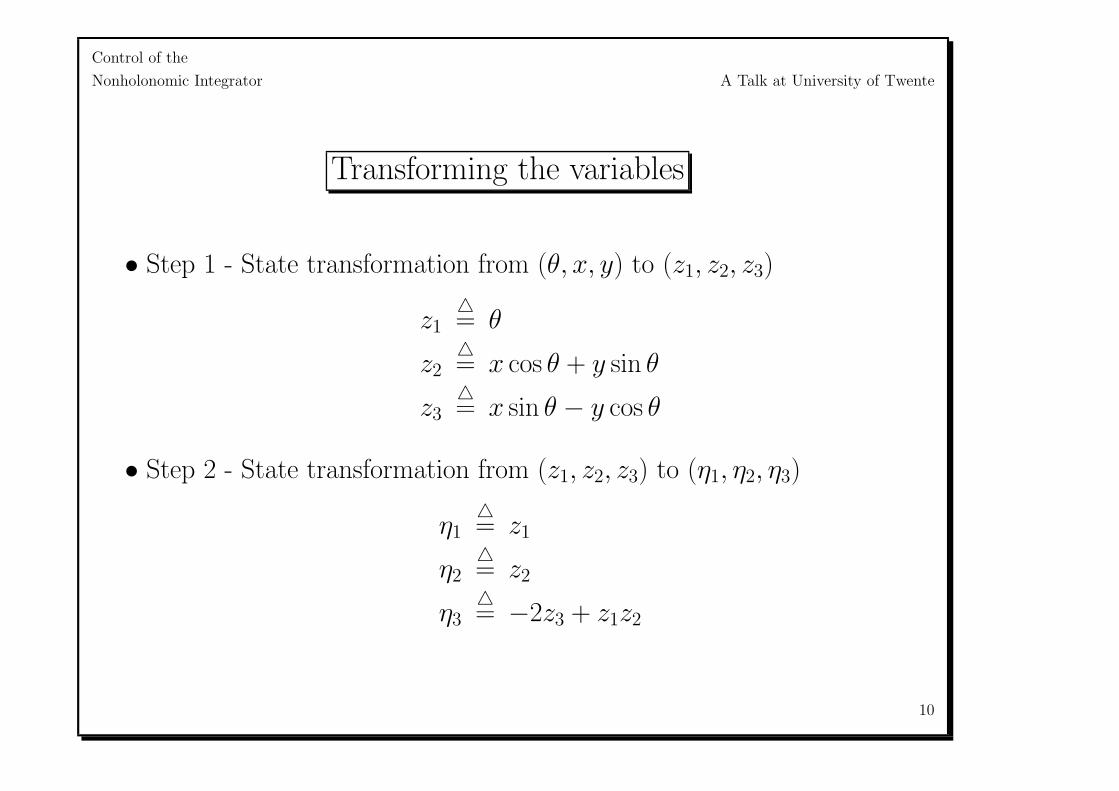
Transforming the variables
• Step 1 - State transformation from (θ, x, y) to (z1, z2, z3)
z1= θ
z2= x cos θ + y sin θ
z3= x sin θ − y cos θ
• Step 2 - State transformation from (z1, z2, z3) to (η1, η2, η3)
η1= z1
η2= z2
η3= −2z3 + z1z2
10

Control of the
Nonholonomic Integrator A Talk at University of Twente
The new representation
• Define modified control inputs as
u1= ω u2
= z3ω + v
• The system in the new states and inputs is η1
η2
η3
=
u1
u2
η1u2 − η2u1
11

Control of the
Nonholonomic Integrator A Talk at University of Twente
Technique 1 - Exponential Stability in a Dense Set
Definition 1.1 If the system is exponentially stable in an open dense
set O, and the control law is well defined and bounded along the closed
loop trajectories, then the closed system is said to be almost
exponentially stable (AES).
• The open dense set in the system under consideration is
O = x ∈ IR3|x1 = 0.
• Proposition 1.1 The NI is AES with the control law
u =
(−k1x1
−k3x3x1− k1x2
)x1 = 0
where 0 < k1 < k3.
12

Control of the
Nonholonomic Integrator A Talk at University of Twente
Proof
• The closed loop dynamics can be written in the form
x = Ax + g(t)
where
A =
−k1 0 0
0 −k1 0
0 0 −k3
; g(t) =
0
−k3x3(t)x1(t)
0
Since g(t) ≤ |k3
x3(0)x1(0)|e(k1−k3)t and the eigen values of A are
negative-real , the system is exponentially stable.
• If x1(0) = 0, then an open loop control can be used to steer the system
to any non zero value of x1 and then the control law can be applied.
13

Control of the
Nonholonomic Integrator A Talk at University of Twente
Technique 2 - Bounded Control Law
• In Technique 1, if the initial condition is close to the surface x1 = 0,
the magnitude of u2 is very large.
• Define α= |x3
x1| and a set
M1= x ∈ IR3 : α ≤ c
and three other sets as
M2= x ∈ IR3 : x /∈ M1 and |x2 + c| ≥ 1
M3= x ∈ IR3 : x /∈ M1 and |x2 + c| < 1
M4= x ∈ IR3 : x1 = x3 = 0
14

Control of the
Nonholonomic Integrator A Talk at University of Twente
Technique 2
• Proposition 1.2 The NI is exponentially stable in the set M1
containing the origin under the following control law
u =
(−k1x1
−k3x3x1− k1x2
)if x ∈ M1(
ksS1/3
x2+c
0
)if x ∈ M2(
0
d
)if x ∈ M3(
−k1x1
−k1x2
)if x ∈ M4
where S(x)= x3 − cx1 and 0 < k1 < k3, 0 < ks and d is any non
zero constant.
15
Control of the
Nonholonomic Integrator A Talk at University of Twente
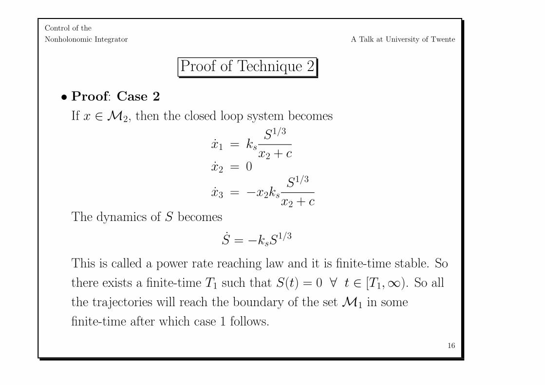
Proof of Technique 2
• Proof: Case 2
If x ∈ M2, then the closed loop system becomes
x1 = ksS1/3
x2 + cx2 = 0
x3 = −x2ksS1/3
x2 + cThe dynamics of S becomes
S = −ksS1/3
This is called a power rate reaching law and it is finite-time stable. So
there exists a finite-time T1 such that S(t) = 0 ∀ t ∈ [T1,∞). So all
the trajectories will reach the boundary of the set M1 in some
finite-time after which case 1 follows.
16

Control of the
Nonholonomic Integrator A Talk at University of Twente
Finite time stabilization to the surface S(x) = 0
• The dynamics of the surface is given by
S = −ksS1/3
• Consider a Lyapunov candidate function and its rate of change
V = S2/2
V = −ksS4/3 < 0
Hence S = 0 is attractive globally.
• For finite time convergence we show
V + kV α ≤ 0 ([Haimo] condition for finite-time stability)
where α ∈ (0, 1) and k > 0
17

Control of the
Nonholonomic Integrator A Talk at University of Twente
• For α = 2/3 and k < 223ks we have
V + kV23 = −S4/3(ks −
k
223
) < 0
• Further
S = 0
which implies that S = 0 is positively invariant
18

Control of the
Nonholonomic Integrator A Talk at University of Twente
Proof
Case 3
If x ∈ M3 , then the dynamics of x2 is
x2 = d
So there exists a finite-time T2 such that |x2(T2) + c| = 1. Then Case 2
follows.
Case 4
If x ∈ M4, then closed loop system becomes
x1 = 0
x2 = −k1x2
x3 = 0
and we have exponential stability
19

Control of the
Nonholonomic Integrator A Talk at University of Twente
Techniques 1 and 2
• Methods 1 and 2 are related though the AES property of 1 does not
hold in 2. Method 2 however guarantees boundedness of the control law
in a local domain around the origin.
20
Control of the
Nonholonomic Integrator A Talk at University of Twente
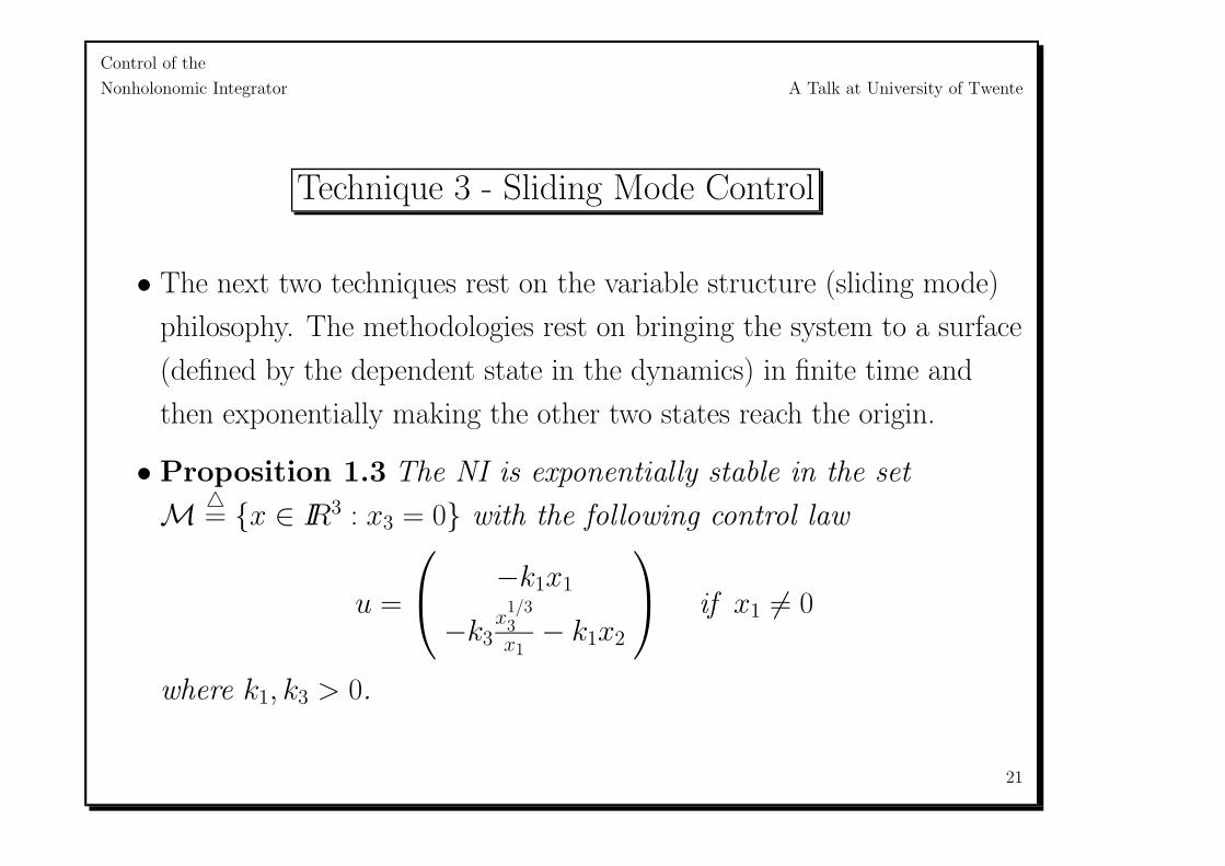
Technique 3 - Sliding Mode Control
• The next two techniques rest on the variable structure (sliding mode)
philosophy. The methodologies rest on bringing the system to a surface
(defined by the dependent state in the dynamics) in finite time and
then exponentially making the other two states reach the origin.
• Proposition 1.3 The NI is exponentially stable in the set
M = x ∈ IR3 : x3 = 0 with the following control law
u =
−k1x1
−k3x
1/33x1
− k1x2
if x1 = 0
where k1, k3 > 0.
21

Control of the
Nonholonomic Integrator A Talk at University of Twente
Proof of Technique 3
• If x1(0) = 0 then the closed loop system is
x1 = −k1x1
x2 =−k3x
1/33
x1− k1x2
x3 = −k3x1/33
Since k1, k3 > 0, the dynamics of x3 implies finite time stability while
that of x1 implies exponential stability. So there exists a finite time
T1 > 0 such that x3(t) ≡ 0 ∀t ≥ T1.
• The system on M is then governed by the set of equations
x1 = −k1x1 x2 = −k1x2 x3 ≡ 0
22

Control of the
Nonholonomic Integrator A Talk at University of Twente
Technique 4
• Define S(x)= x2
1 − 3k1x2/33 where k1 > 0 is a predefined constant,
• Proposition 1.4 The NI is exponentially stable in the set
M = x ∈ IR3 : x3 = 0 with the following time-varying control
law
u =
(−k1x1
−x1x1/33 − k1x2
)∀ s ∈ [t,∞) if S(x(t)) > 0(
x1
x2
)if S(x(t)) ≤ 0(
−k1x1
−k1x2
)if x3 = 0
23

Control of the
Nonholonomic Integrator A Talk at University of Twente
Proof of Technique 4
Case 1 Assume S(x(0)) > 0
• We have
x1 = −k1x1
x2 = −x1x1/33 − k1x2
x3 = −x21x
1/33
• The evolution of x1(t) is given by
x1(t) = x1(0)e−k1t
• The evolution of x3 is
x3(t) = ±[x1(0)2e−2k1t − S(x(0))
3k1]3/2 ∀t ∈ [0, T1)
x3(t) = 0 ∀t ≥ T1
24
Control of the
Nonholonomic Integrator A Talk at University of Twente
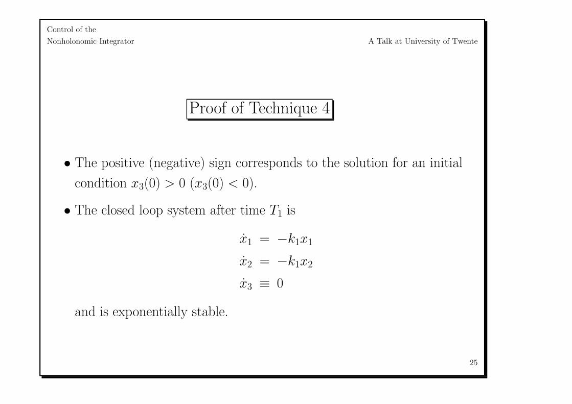
Proof of Technique 4
• The positive (negative) sign corresponds to the solution for an initial
condition x3(0) > 0 (x3(0) < 0).
• The closed loop system after time T1 is
x1 = −k1x1
x2 = −k1x2
x3 ≡ 0
and is exponentially stable.
25

Control of the
Nonholonomic Integrator A Talk at University of Twente
Proof of Technique 4
• Case 2 If x1(0) = 0 and S(x(0)) ≤ 0 , then we have
x1 = x1
x2 = x2
x3 = 0
The above dynamics leads to an increase in the value of S(x(t)) as time
increases. Note that x3 remains a constant and x1 has an exponential
growth. So there exists a finite-time such that S(x(t)) > 0. Then Case
1 follows.
26

Control of the
Nonholonomic Integrator A Talk at University of Twente
• The third case is straightforward. If x1(0) = 0 then any open loop
control can push x1 to some non-zero value, then either case 1 or case 2
follows.
27

Control of the
Nonholonomic Integrator A Talk at University of Twente
Techniques 3 and 4
• Methods 3 and 4 bring in a variable structure (or sliding mode) feature;
the latter is also time-varying.
• Both techniques use a power rate reaching law to enter a set in which
the system is exponentially stable.
• The idea in Method 4 is to utilize the state x1 as a gain for the
convergence of x3 to zero in finite-time. So we have the term x1x1/33
instead ofx
1/33x1
. But since this control law valid in a local domain, we
have introduced a swtiching strategy to move from anywhere to this
domain.
• All the four control laws are not defined for x1(0) = 0.
28

Control of the
Nonholonomic Integrator A Talk at University of Twente
• Closest parallels - notions of sigma process, paper by Bloch and
Drakunov
29

Control of the
Nonholonomic Integrator A Talk at University of Twente
Dynamic model of the mobile robot
• θ
x
y
v
ω
=
ω
v cos θ
v sin θ
0
0
+
0
0
01M
0
F +
0
0
0
01I
τ
• Fifth order system with drift
• Discontinuous controllers (velocity level) designed from the kinematic
model cannot be applied to obtain controllers at the acceleration level
for the dynamic model.
30

Control of the
Nonholonomic Integrator A Talk at University of Twente
Transforming the variables
• Step 1 - State transformationz1
z2
z3
z4
z5
=
θ
x cos θ + y sin θ
x sin θ − y cos θ
ω
v − (x sin θ − y cos θ)ω
• The dynamic model in the z variables
z1
z2
z3
z4
z5
=
z4
z5
z2z4
τI
FM − τ
I z3 − z2z24
31

Control of the
Nonholonomic Integrator A Talk at University of Twente
Transforming the variables
• Alternate inputs
u1=
τ
Iu2
= −z2
4z2 −τ
Iz3 +
F
M
• Step 2 - State transformation from (z1, z2, z3, z4, z5) to
(x1, x2, x3, y1, y2)
x1= z1 x2
= z2 x3
= −2z3 + z1z2 y1
= z4 y2
= z5
• The system equations are now in the form
x1 = u1
x2 = u2
x3 = x1x2 − x2x1
32
Control of the
Nonholonomic Integrator A Talk at University of Twente
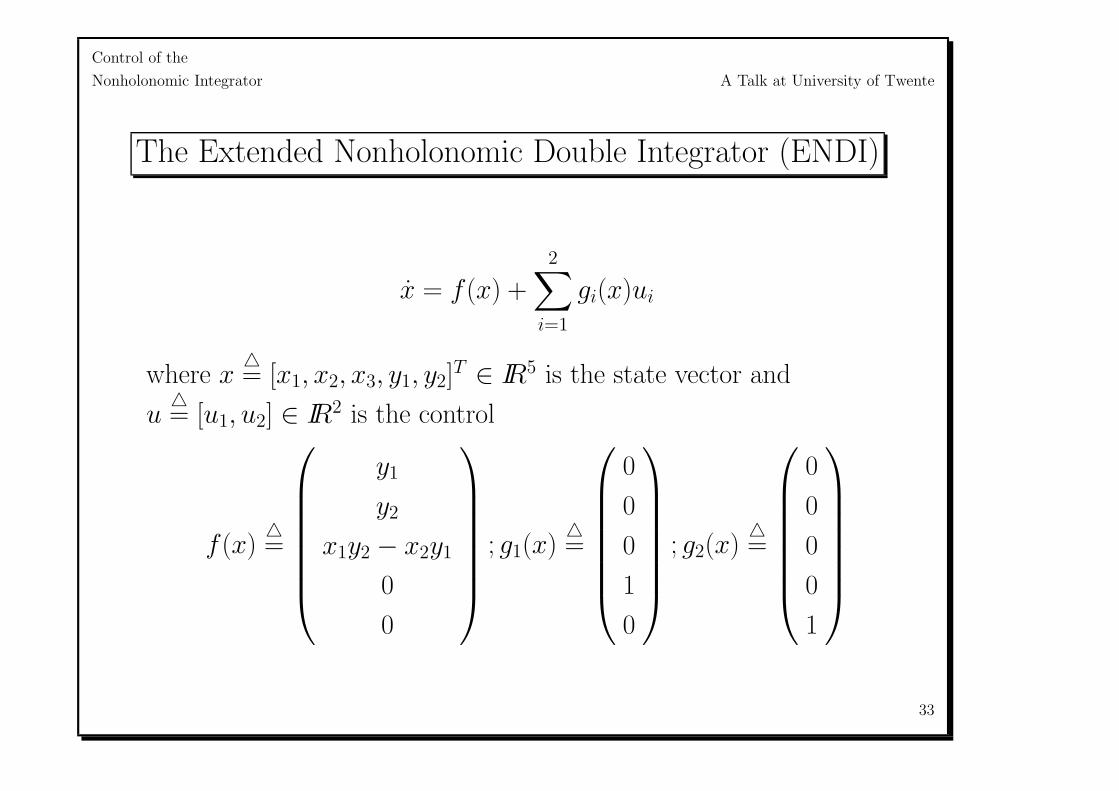
The Extended Nonholonomic Double Integrator (ENDI)
x = f (x) +
2∑i=1
gi(x)ui
where x= [x1, x2, x3, y1, y2]
T ∈ IR5 is the state vector and
u= [u1, u2] ∈ IR2 is the control
f (x)=
y1
y2
x1y2 − x2y1
0
0
; g1(x)=
0
0
0
1
0
; g2(x)=
0
0
0
0
1
33

Control of the
Nonholonomic Integrator A Talk at University of Twente
Features of the ENDI
• The equlibria of the ENDI system are of the form
xe = x ∈ IR5 : y1 = y2 = 0 and satisfy the following properties
1. xe is not stabilized by any smooth feedback control laws.
2. The ENDI is locally strongly accessible from any x ∈ IR5.
3. The ENDI is small time locally controllable (STLC) from any xe.
34

Control of the
Nonholonomic Integrator A Talk at University of Twente
A Sliding Mode Approach
• Define S1(x)= kx1 + y1 and S2(x)
= x1y2 − x2y1 + k3x3 where
k3 > k > 0
• Define the sets
M1= x ∈ IR5 : S1(x) = 0 M2
= x ∈ M1 : S2(x) = 0
• Proposition 1.5 The origin of the ENDI is exponentially stable in
the set M2 with the following control law
u1 = −ky1 − S1/31 if (x1, y1) = 0
u2 =
−S1/32
x1− k3y2 − (k3 − k)kx2 x ∈ M1 (x = 0)
−x2 − y2 otherwise
35

Control of the
Nonholonomic Integrator A Talk at University of Twente
Proof
• The closed loop dynamics for (x1, y1) = 0 and x /∈ M1 becomes
x1 = y1
x2 = y2
x3 = x1y2 − x2y1
y1 = −ky1 − S1(x)1/3
y2 = −x2 − y2
• The dynamics of S1(x) is
S1 = −S1/31
and the surface S1(x) = 0 is finite-time stable
36

Control of the
Nonholonomic Integrator A Talk at University of Twente
• So there exists a time T1 ≥ 0 such that the closed loop trajectory for
any permissible initial condition reaches the set M1 and stays there for
all future time. The control law u1 allows both x1 and y1 to converge
to zero as time gets large.
• At the same time as the system is being driven towards M1, the PD
control law u2 with unity gain makes states x2 and y2 converge to zero.
37

Control of the
Nonholonomic Integrator A Talk at University of Twente
The dynamics on the set M1
• The closed loop system on M1 is
x1 = −kx1
x2 = y2
x3 = x1y2 − x2y1
y1 = −ky1
y2 =−S
1/32
x1− k3y2 − (k3 − k)kx2
• The dynamics of S2 is
S2 = −S1/32
So there exists a time T2 ≥ T1 ≥ 0 such that the closed loop
trajectories reach the set M2 and stay there for all future time.
38

Control of the
Nonholonomic Integrator A Talk at University of Twente
The dynamics on the set M2
• The closed loop system on M2
x1 = −kx1
x2 = y2
x3 = −x3
y1 = −ky1
y2 = −k3y2 − (k3 − k)kx2
• All trajectories converge to the origin
39

Control of the
Nonholonomic Integrator A Talk at University of Twente
Simulation
• Initial conditions are x(0) = −1.5m, y(0) = 4m, θ(0) =
−2.3rad, ω(0) = 1rad/sec, v(0) = −1m/sec.
• Controller parameters are k = 0.5, k3 = 1.
• Vehicle parameters are
M = 10Kg, I = 2Kgm2, L = 6cm, R = 3cm.
40

Control of the
Nonholonomic Integrator A Talk at University of Twente
−5 −4 −3 −2 −1 0 1 2 3 4 5−5
−4
−3
−2
−1
0
1
2
3
4
5
intial condition
x in meters
y in
met
ers
Figure 3: Stabilization to the origin
41

Control of the
Nonholonomic Integrator A Talk at University of Twente
0 10 20 30 40 50−3
−2
−1
0
1
2
3
4
5
time in sec
x,y
in m
eter
s, θ
in r
ad
xyθ
Figure 4: Position and orientation of the vehicle
42

Control of the
Nonholonomic Integrator A Talk at University of Twente
0 10 20 30 40 50−1
−0.5
0
0.5
1
1.5
time in sec
v in
m/s
ec, ω
in r
ad/s
ec
ωv
Figure 5: Velocities of the vehicle
43

Control of the
Nonholonomic Integrator A Talk at University of Twente
0 10 20 30 40 50−0.2
−0.15
−0.1
−0.05
0
0.05
0.1
0.15
time in sec
τ 1,τ2 in
Nm
τ1τ2
Figure 6: Input to the motors
44

Control of the
Nonholonomic Integrator A Talk at University of Twente
Thank You
45


![[1] Developments in Nonholonomic Control Problems](https://static.fdocuments.us/doc/165x107/55cf983e550346d0339674aa/1-developments-in-nonholonomic-control-problems.jpg)
