Control of Manufacturing Processes · Control of Manufacturing Processes Subject 2.830 Spring 2003...

Control of Manufacturing Control of Manufacturing ProcessesProcesses

Subject 2.830Subject 2.830Spring 2003Spring 2003Lecture #9Lecture #9

““SPC Charting and Process Capability"SPC Charting and Process Capability"March 4, 2004March 4, 2004

3/4/04 Lecture 9 © D.E. Hardt, all rights reserved 2

The SPC HypothesisThe SPC Hypothesis

...

...

In-Control

Not

In-Control

0

0.1

0.2

0.3

0.4

0.5

0.6

0.7

0.8

0.9

1 2 3 4 5 6 7 8 9 10 11 12 13 14 15 16 17 18 19 20Sample Number

Process Y

p(y)


Example xbarExample xbar

0

0.1

0.2

0.3

0.4

0.5

0.6

0.7

0.8

0.9

1

1 2 3 4 5 6 7 8 9 10 11 12 13 14 15 16 17 18 19 20sample number

UCL

LCL

Grand

Mean


Western Electric Rules Western Electric Rules (See Table 4(See Table 4--1)1)

•• Points outside limitsPoints outside limits•• 22--3 consecutive points outside 2 sigma3 consecutive points outside 2 sigma•• Four of five consecutive points beyond Four of five consecutive points beyond

1 sigma1 sigma•• Run of 8 consecutive points on one side Run of 8 consecutive points on one side

of centerof center


Out of ControlOut of Control•• Data is not Stationary Data is not Stationary

((µµ or or σσ are not constant)are not constant)

•• Process Output is being “caused” by a Process Output is being “caused” by a disturbance (assignable or special cause)disturbance (assignable or special cause)

•• This disturbance can be identified and This disturbance can be identified and eliminatedeliminated–– Trends indicate certain typesTrends indicate certain types–– Correlation with know eventsCorrelation with know events

•• shift changesshift changes•• material changesmaterial changes


Design of the ChartDesign of the Chart•• Sample size nSample size n

–– Central Limit theoremCentral Limit theorem–– ARL effects?ARL effects?

•• Sample time Sample time ∆∆TT–– Cost of samplingCost of sampling–– production without dataproduction without data–– Rapid phenomenaRapid phenomena

•• Selection of Reference DataSelection of Reference Data–– Is S at a minimum ?

Sample size and “filtering” versus response

time to changes

Is S at a minimum ?


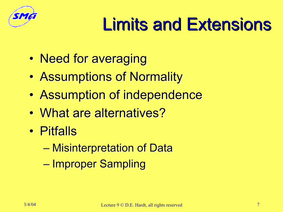
Limits and ExtensionsLimits and Extensions

•• Need for averagingNeed for averaging•• Assumptions of NormalityAssumptions of Normality•• Assumption of independenceAssumption of independence•• What are alternatives?What are alternatives?•• PitfallsPitfalls

–– Misinterpretation of DataMisinterpretation of Data–– Improper SamplingImproper Sampling


Use of the S ChartUse of the S Chart

•• Plot of sample VariancePlot of sample Variance–– Variance of the Mean for Shewhart xbar Variance of the Mean for Shewhart xbar

(n>1)(n>1)

•• What Does it Tell Us about State of What Does it Tell Us about State of Control?Control?–– It simply plots the “other” statistic It simply plots the “other” statistic


Consider this Process Consider this Process Xbar ChartXbar Chart

0

0.1

0.2

0.3

0.4

0.5

0.6

0.7

0.8

0.9

1

1 2 3 4 5 6 7 8 9 10 11 12 13 14 15 16 17 18 19 20

sample number

UCL

LCL


And the S ChartAnd the S Chart

0

0.1

0.2

0.3

0.4

0.5

0.6

1 2 3 4 5 6 7 8 9 10 11 12 13 14 15 16 17 18 19 20

UCL

LCL


In Control?In Control?


Same Process Later in TimeSame Process Later in Time

0

0.1

0.2

0.3

0.4

0.5

0.6

0.7

0.8

0.9

1

1 2 3 4 5 6 7 8 9 10 11 12 13 14 15 16 17 18 19 20

sample number

UCL

LCL

Xbar


Later S ChartLater S Chart

0

0.1

0.2

0.3

0.4

0.5

0.6

1 2 3 4 5 6 7 8 9 10 11 12 13 14 15 16 17 18 19 20

UCL

LCL


What Changed??What Changed??


A Different SequenceA Different Sequence

0

0.1

0.2

0.3

0.4

0.5

0.6

0.7

0.8

0.9

1

1 2 3 4 5 6 7 8 9 10 11 12 13 14 15 16 17 18 19 20

sample number

UCL

LCL

Xbar


S ChartS Chart

0

0.1

0.2

0.3

0.4

0.5

0.6

1 2 3 4 5 6 7 8 9 10 11 12 13 14 15 16 17 18 19 20

UCL

LCL


Use of S ChartUse of S Chart

•• Detect Changes in Variance of Parent Detect Changes in Variance of Parent DistributionDistribution

•• Distinguish Between Mean and Distinguish Between Mean and Variance ChangesVariance Changes


Statistical Process ControlStatistical Process Control

•• Model Process as a Normal Model Process as a Normal Independent*Independent*Random VariableRandom Variable

•• CompletelyCompletely described by described by µµ and and σσ•• Estimate using Estimate using xbaxbar and r and ss•• Enforce Stationary ConditionsEnforce Stationary Conditions•• Look for Deviations in Either StatisticLook for Deviations in Either Statistic•• If so ………..?If so ………..?•• Call an Engineer!Call an Engineer!


Another Use of the Another Use of the Statistical Process Model: Statistical Process Model:

The Manufacturing The Manufacturing --Design InterfaceDesign Interface•• We now have an empirical model of the We now have an empirical model of the

processprocess

0

0.05

0.1

0.15

0.2

0.25

0.3

0.35

0.4

0.45

-4 -3 -2 -1 0 1 2 3 4

µ +3σ−3σ

How “good” is the process?

Is it capable of producing what we need?


Process CapabilityProcess Capability

•• Assume Process is InAssume Process is In--controlcontrol•• Described fully by Described fully by xbarxbar and and ss•• Compare to Design SpecificationsCompare to Design Specifications

–– TolerancesTolerances–– Quality LossQuality Loss


Design SpecificationsDesign Specifications

•• TolerancesTolerances: Upper and Lower Limits: Upper and Lower Limits

CharacteristicDimension

Targetx*

Upper Specification Limit

USL

Lower Specification Limit

LSL


Design SpecificationsDesign Specifications

•• Quality LossQuality Loss: Penalty for Any Deviation : Penalty for Any Deviation from Targetfrom Target

QLF = L*(x-x*)2

x*=target

How to How to Calibrate?Calibrate?


Use of Tolerances:Use of Tolerances:Process CapabilityProcess Capability

0

0.05

0.1

0.15

0.2

0.25

0.3

0.35

0.4

0.45

-4 -3 -2 -1 0 1 2 3 4µ +3σ−3σx* USLLSL

•• Define Process using a Normal DistributionDefine Process using a Normal Distribution•• Superimpose x*, LSL and USLSuperimpose x*, LSL and USL•• Evaluate Expected PerformanceEvaluate Expected Performance



•• DefinitionsDefinitions

•• Compares ranges onlyCompares ranges only•• No effect of a mean shift:No effect of a mean shift:

Cp =(USL − LSL)

6σ=

tolerance range99.97% confidence range


= Minimum of the normalized = Minimum of the normalized deviation from the meandeviation from the mean

•• Compares effect of offsetsCompares effect of offsets

Cpk = min(USL − µ)

3σ,(LSL − µ)

3σ⎛ ⎝

⎞ ⎠

Process Capability: CProcess Capability: Cpkpk


Cp = 1; Cpk = 1Cp = 1; Cpk = 1

0

0.05

0.1

0.15

0.2

0.25

0.3

0.35

0.4

0.45

-4 -3 -2 -1 0 1 2 3 4


Cp = 1; Cpk = 0Cp = 1; Cpk = 0

0

0.05

0.1

0.15

0.2

0.25

0.3

0.35

0.4

0.45

-4 -3 -2 -1 0 1 2 3 4


Cp = 2; Cpk = 1Cp = 2; Cpk = 1

0

0.05

0.1

0.15

0.2

0.25

0.3

0.35

0.4

0.45

-4 -3 -2 -1 0 1 2 3 4


Cp = 2; Cpk = 2Cp = 2; Cpk = 2

0

0.05

0.1

0.15

0.2

0.25

0.3

0.35

0.4

0.45

-4 -3 -2 -1 0 1 2 3 4


Effect of ChangesEffect of Changes

•• In Design SpecsIn Design Specs•• In Process MeanIn Process Mean•• In Process VarianceIn Process Variance

•• What are good values of Cp and Cpk?What are good values of Cp and Cpk?


Cpk Table Cpk Table

Cpk z P<LS orP>USL

1 3 1E-031.33 5 3E-071.67 4 3E-05

2 6 1E-09


The The ““6 Sigma6 Sigma”” problemproblem

0

0.05

0.1

0.15

0.2

0.25

0.3

0.35

0.4

0.45

-4 -3 -2 -1 0 1 2 3 4

+3σ∗−3σ∗

P(x > 6σ) = 18.8x10-10 Cp=2

Cpk=2

LSL USL

6σ


The 6 The 6 σσ problem: Mean Shifts problem: Mean Shifts

0

0.05

0.1

0.15

0.2

0.25

0.3

0.35

0.4

0.45

-4 -3 -2 -1 0 1 2 3 4

USL

P(x>4σ) = 31.6x10-6 Cp=2

Cpk=4/3Even with a mean shift of 2σ

we have only 32 ppm out of spec

LSL

4σ


QLF = L(x) =k*(x-x*)2

Capability from the Quality Capability from the Quality Loss FunctionLoss Function

x*Given L(x) and p(x) what is E{L(x)}?


Expected Quality LossExpected Quality Loss

E{L(x)}= E k(x − x*)2[ ]= k E(x2 ) − 2E(xx*) + E(x *2 )[ ]= kσ x

2 + k(µx − x*)2

Penalizes Variation

Penalizes Deviation



•• The reality (the process statistics)The reality (the process statistics)•• The requirements (the design specs)The requirements (the design specs)•• Cp Cp -- a measure of variance vs. a measure of variance vs.

tolerancetolerance•• Cpk a measure of variance from targetCpk a measure of variance from target•• Expected LossExpected Loss-- An overall measure of An overall measure of

goodnessgoodness

Control of Manufacturing Processes · Control of Manufacturing Processes Subject 2.830 Spring 2003...

Documents

Transcript of Control of Manufacturing Processes · Control of Manufacturing Processes Subject 2.830 Spring 2003...