C

Ya

b

ontrol of industrial gas phase propylene polymerization in fluidized bed reactors

ong Kuen Hoa, Ahmad Shamiri a, Farouq S. Mjalli b,∗, M.A. Hussaina

Chemical Engineering Department, Faculty of Engineering, University of Malaya, 50603 Kuala Lumpur, MalaysiaPetroleum & Chemical Engineering Department, Sultan Qaboos University, Muscat 123, Oman

a b s t r a c t

The control of a gas phase propylene polymerization model in a fluidized bed reactor was studied, wherethe rigorous two phase dynamic model takes into account the polymerization reactions occurring in thebubble and emulsion phases. Due to the nonlinearity of the process, the employment of an advancedcontrol scheme for efficient regulation of the process variables is justified. In this case, the Adaptive Pre-dictive Model-Based Control (APMBC) strategy (an integration of the Recursive Least Squares algorithm,RLS and the Generalized Predictive Control algorithm, GPC) was employed to control the polypropyleneproduction rate and emulsion phase temperature by manipulating the catalyst feed rate and reactor cool-

ing water flow, respectively. Closed loop simulations revealed the superiority of the APMBC in setpointtracking as compared to the conventional PI controllers tuned using the Internal Model Control (IMC)method and the standard Ziegler–Nichols (Z–N) method. Moreover, the APMBC was able to efficientlyarrest the effects of superficial gas velocity, hydrogen concentration and monomer concentration on theprocess variables, thus exhibiting excellent regulatory control properties.

.

1. Introduction

The production of polypropylene in fluidized bed reactors is oneof the most widely used technologies in the polymerization indus-try. However, the complicated reaction, heat and mass transfermechanisms as well as the complex gas and solid flow characteris-tics in the reactor introduce extreme nonlinearities in the dynamicsof the reactor. As such, the modelling and control of such a processis a huge challenge. The fundamental control problem in the propy-lene polymerization fluidized bed reactor is further complicatedby the existence of strong interaction between reactor variables;of which conventional process control strategies are incapableof coping. Although there are studies reported in the academic

∗ Corresponding author. Tel.: +968 93284366.E-mail address: farouqsm@yahoo.com (F.S. Mjalli).

literature on the modelling and control of polymerization process influidized bed reactors [1–5], little work was done on the modellingand control of specifically the gas phase fluidized bed polypropy-lene reactor.

The simplified schematic of an industrial gas phase fluidizedbed polypropylene reactor is shown in Fig. 1. In the polymeriza-tion reactor, growing polymer particles are fluidized by a recyclegas stream containing propylene monomer, hydrogen and nitrogenThe feed gas flow, which provides the monomer for polymerizationin the presence of Ziegler–Natta catalyst and triethyl aluminumco-catalyst, serves to agitate the bed and fluidization through thedistributor while at the same time removing the heat of polymer-ization from the reactor. The recycle gas, which exits from the topof the reactor is then compressed and cooled before being fed intothe bottom of the fluidized bed.

Due to the highly exothermic nature of the propylene polymer-ization reactions, the cooling of the recycle gas which exits from the

Nomenclature

a(z−1) polynomial associated with y(k) in the CARIMAmodel

A cross sectional area of the reactor (m2)Ar Archimedes numberb(z−1) polynomial associated with u(k) in the CARIMA

modelC VFF-RLS design constantCH hydrogen concentration (kmol/m3)CM Propylene (monomer) concentration (kmol/m3)Cpi specific heat capacity of component i (J/kg K)Cpg specific heat capacity of gaseous stream (J/kg K)Cp,pol specific heat capacity of solid product (J/kg K)db bubble diameter (m)dp particle diameter (m)D diagonal matrixDg gas diffusion coefficient (m2/s)Dt reactor diameter (m)Fcat catalyst feed rate (g/s)Fcw cooling water flow rate (g/s)H matrix associated with the future slew rates in the

GPC prediction equationHbe bubble to emulsion heat transfer coefficient

(W/m3 K)Hbc bubble to cloud heat transfer coefficient (W/m3 K)Hce cloud to emulsion heat transfer coefficient (W/m3 K)j active site typek positive integer denoting the sampling instancekfh (j) transfer rate constant for a site of type j with termi-

nal monomer M reacting with hydrogenkg gas thermal conductivity (W/m K)kp (j) propagation rate constant for a site of type j with

terminal monomer M reacting with monomer MK matrix associated with the past slew rates in the GPC

prediction equationKbc bubble to cloud mass transfer coefficient (s−1)Kbe bubble to emulsion mass transfer coefficient (s−1)Kc proportional gainKce cloud to emulsion mass transfer coefficient (s−1)[Mi] concentration of component i in the reactor

(kmol/m3)[Mi]in concentration of component i in the inlet gaseous

streamMi ith componentMw monomer molecular weight (kg/kmol)N1 minimum prediction horizonN2 maximum prediction horizonNINT[•] nearest integer to [•]NS number of active site typesM control horizonp covariance matrixP pressure (Pa)Q matrix associated with the past outputs in the GPC

prediction equationR move suppression weight for the slew rateRi instantaneous rate of reaction for monomer i

(kmol/s)R(j) rate at which monomer M is consumed by propaga-

tion reactions at sites of type jRemf Reynolds number of particles at minimum fluidiza-

tion conditionR positive definite diagonal weighting matrices con-

taining R

r→k

vector of future setpoints

Rp production rate (kg/s)Rpb bubble phase production rate (kg/s)Rpe emulsion phase production rate (kg/s)Rv volumetric polymer phase outflow rate from the

reactor (m3/s)t time (s)ts sampling timeT temperature (K)Td discrete dead timeTin temperature of the inlet gaseous stream (K)T(z−1) design polynomial in the CARIMA modelU upper triangular matrixU0 superficial gas velocity (m/s)Ub bubble velocity (m/s)Ue emulsion gas velocity (m/s)u(k) process inputUmf minimum fluidization velocity (m/s)v(k) stochastic noise variable with random distribution

and zero meanV reactor volume (m3)Vb volume of the bubble phase (m3)Ve volume of the emulsion phase (m3)Vp volume of polymer phase in the reactor (m3)Vpb volume of polymer phase in the bubble phase (m3)Vpe volume of polymer phase in the emulsion phase

(m3)VPFR volume of plug flow reactor (PFR) (m3)W weight for the output residualW positive definite diagonal weighting matrices con-

taining Wy(k) process outputy→k

vector of future outputs (not including current

value)y←k

vector of past outputs (including current value)

Y(n,j) nth moment of chain length distribution for livingpolymer produced at a site of type j

Greek letters�HR heat of reaction (J/kg)�u change in the input variable (or slew rate)�u→k−1

vector of future slew rates (not including current

value)�u←k−1

vector of past slew rates (including current value)

˛ order of the a(z−1) polynomial order of the b(z−1) polynomial

ı volume fraction of bubbles in the bed� Kalman gain� forgetting factor�d dead time of the processε prediction errorεb void fraction of bubble for Geldart B particlesεe void fraction of emulsion for Geldart B particlesεmf void fraction of the bed at minimum fluidization� gas viscosity (Pa s)� density (kg/m3)�g gas density (kg/m3)�pol polymer density (kg/m3)� VFF-RLS design constant� regressor vector� vector of the estimated process model parameters

D derivative time constantI integral time constant

Subscripts and superscripts1 propylene2 hydrogenb bubble phasee emulsion phaseg gas mixture propertyi component type numberin inletj active site type numbermf minimum fluidizationpol polymer

tpgiatawmtIbac

tasmtlpwstcgbsetbfstrCdca

pimhgi

ref reference condition

op of the reactor (as described above) is crucial to maintaining theolypropylene production rate. The heat removal from the recycleas through the cooler in this system is governed by the heat capac-ty, dew point, and the temperature of the recycle gas. To maintaincceptable polymer production rate (which is an important goal forhe industry), it is necessary to keep the reactor bed temperaturebove the dew point of the reactants to avoid condensation of gasithin the reactor. At the same time, the reactor bed temperatureust also be below the melting point of the polymer to prevent par-

icle melting, agglomeration and consequently reactor shut down.n view of the various stringent operating conditions required, sta-ilization of propylene polymerization in fluidized bed reactors is

challenging task which can only be addressed through efficientontrol system design.

For the fluidized bed polymerization reactor, most of the reac-or design and control problems are associated with achievingdequate production rate and heat removal from the reactor. Theteady state and dynamic behavior of the reactor is influenced byany process variables such as the superficial gas velocity, feed gas

emperature, monomer concentration, catalyst activity, and cata-yst feed rate, etc. The first attempt in describing the dynamics ofropylene polymerization was done by Choi and Ray [1]. In theirork, two phases, viz. the bubble and emulsion phases were con-

idered in the proposed dynamic model. Furthermore, it was shownhat the employment of a PI feedback control scheme was capable ofontrolling the process transients, albeit still limited by the recycleas cooling capacity. Ibrehem et al. [4] proposed that the fluidizeded comprise four phases, namely the bubble, cloud, emulsion andolid phases, with polymerization reactions occurring only in themulsion and solid phases. In the same work, the temperature ofhe polyethylene system was controlled by using a neural networkased predictive controller. Moreover, it was shown that the per-ormance of the neural network based predictive controller wasuperior to the conventional PID controller in terms of setpointracking. In another study on industrial gas phase polyethyleneeactors, Dadebo et al. [2] showed the nonlinear Error Trajectoryontroller (ETC) exhibited superior responses in terms of speed,amping and robustness as compared to an optimally tuned PIDontroller for the control of temperature over a wide range of oper-ting conditions.

In the present study, the control of a newly proposed twohase dynamic model for homo-polymerization of propylene in flu-

dized bed reactors will be investigated. In the proposed dynamic

odel, the presence of solid particles in the bubble phase (which

as been validated experimentally [6–8]) as well as the excessas in the emulsion phase [7–9] and polymerization reactionn both phases are considered to realistically mimic the actual

polymerization process which occurs in the fluidized bed reactor[7,8]. In short, the present model takes into account the poly-merization reactions which occur in two phases. In this system,the reactor temperature is controlled by manipulating the coolingwater flow rate of an upstream heat exchanger, which consequentlyremoves the heat produced by the exothermic polymerization reac-tions from the recycle gas stream [2]. Concurrently, changes tothe catalyst feed rate and the bed level can be used to controlboth the polymer production rate and the solid phase residencetime [10]. The catalyst injection and product withdrawal rates areadjusted in such a way that maintains a constant bed level inside thereactor.

In this work, adaptive control strategy was employed to dealwith the control issue of the polypropylene fluidized bed reac-tor. Due to the high nonlinearities involved in the dynamics of thepolymerization reactor, it is therefore beyond the capability of theconventional PID controller with fixed controller settings to achieveexcellent control of the reactor variables. In order to achieve goodcontrol of the reactor variables, a more intelligent and efficientprocess control scheme is needed, where the controller is able toautomatically re-design itself in real time according to the chang-ing process dynamics. Such a controller which can readjust itself(i.e. the controller settings are updated in real time according tothe most recent process dynamics) is referred to as “adaptive con-trollers”. Where nonlinearities are concerned, adaptive controllersare known to be adept in handling such difficult process controlscenarios [11,12].

Among the multitudes of adaptive control techniques availableto date, the self-tuning approach has received the most attentionin the past decades [13–15]. In this approach, the controller isdesigned in real time to adapt to the most recent dynamics of theprocess based on the output of a recursive system identificationprocedure (i.e. the estimated process model parameters). Ljung andSöderstöm [16] presented a number of mathematical algorithmswhich can be used for identifying a system recursively. Amongthese, Seborg et al. [13] reported that the Recursive Least Squares(RLS) algorithm and the Extended Least Squares (ELS) algorithmare the two most commonly used recursive system identificationalgorithms in adaptive control. However, the use of the RLS algo-rithm (i.e. the choice of recursive system identification techniquein this study) in adaptive control is comparatively more popularthan the ELS algorithm due to its simplicity and rapid convergencewhen properly applied. Given the real time data of the inputs andthe outputs of a process, the RLS algorithm produces sequentialupdates of the process model parameters, which can be used sub-sequently in controller design. Although the success of RLS-basedadaptive controllers in controlling polymerization reactors (boththe lab scale as well as the industrial scale) is evident in the lit-erature [17–21], there is virtually no published work to date aspertaining to the control of a gas phase propylene polymerizationfluidized bed reactor.

The choice of the control algorithm to be coupled to the RLSalgorithm is of equal importance to the recursive system identi-fication component in the design of an adaptive controller. In thisstudy, the Model Predictive Control (MPC) technology, specificallythe linear Generalized Predictive Control (GPC) strategy is selectedas the choice of control algorithm. Although the first principlepolymerization model can be used with the nonlinear MPC tocontrol the process, this is not done in this work as the mechanisticpolypropylene polymerization process model is overly compli-cated (e.g. with excessive number of states, etc.) to be used withina model based framework. In our case, the internal model used by

the GPC for predictive calculations is regenerated at every controlinterval by the RLS algorithm. In essence, the nonlinear processis continuously being identified by the RLS algorithm in the formof an instantaneous linear model which can be used by the GPC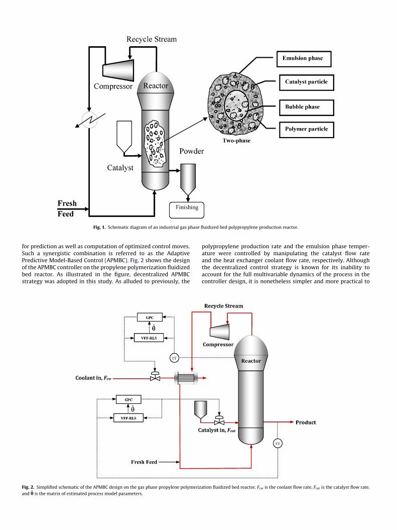

hase fl

fSPobs

Fa

Fig. 1. Schematic diagram of an industrial gas p

or prediction as well as computation of optimized control moves.uch a synergistic combination is referred to as the Adaptiveredictive Model-Based Control (APMBC). Fig. 2 shows the design

f the APMBC controller on the propylene polymerization fluidizeded reactor. As illustrated in the figure, decentralized APMBCtrategy was adopted in this study. As alluded to previously, the

ig. 2. Simplified schematic of the APMBC design on the gas phase propylene polymerizand � is the matrix of estimated process model parameters.

uidized bed polypropylene production reactor.

polypropylene production rate and the emulsion phase temper-ature were controlled by manipulating the catalyst flow rateand the heat exchanger coolant flow rate, respectively. Although

the decentralized control strategy is known for its inability toaccount for the full multivariable dynamics of the process in thecontroller design, it is nonetheless simpler and more practical to

tion fluidized bed reactor. Fcw is the coolant flow rate, Fcat is the catalyst flow rate,

Table 1Correlations and equations used in the two-phase model.

Parameter Formula Reference

Minimum fluidization velocity Remf = [(29.5)2 + 0.357Ar]1/2 − 29.5 [41]

Bubble velocity Ub = U0 − Ue + ubr [42]Bubble rise velocity ubr = 0.711(gdb)1/2 [42]

Emulsion velocity Ue = U0−ıUb1−ı

[43]

Bubble diameter db = db0[1 + 27(U0 − Ue)]1/3(1 + 6.84H) [44]db0 = 0.0085 (for Geldart B)

Kbe =(

1Kbc+ 1

Kce

)−1

Mass transfer coefficient Kbc = 4.5(

Uedb

)+ 5.85

(Dg

1/2g1/4

db5/4

)[42]

Kce = 6.77(

Dg εeubrdb

)Heat transfer coefficient Hbe =

(1

Hbc+ 1

Hce

)−1[42]

Hbc = 4.5(

Ue�g Cpgdb

)+ 5.85 (kg �g Cpg )1/2g1/4

db5/4

Hce = 6.77(�gCpgkg )1/2(

εeubr

db3

)1/2

Bubble phase fraction ı = 0.534[

1 − exp(− U0−Umf

0.413

)][7]

Emulsion phase porosity εe = εmf + 0.2 − 0.059 exp(− U0−Umf

0.429

)[7]

Bubble phase porosity εb = 1 − 0.146 exp(− U0−Umf

4.439

)[7]

Volume of polymer phase in the emulsion phase VPe = Ah(1 − εe)(1 − ı) [23] Ah(1

A(1 − AıH

idwapfc

pmbsfmcM

2

pesud

TR

Volume of polymer phase in the bubble phase VPb =Volume of the emulsion phase Ve =Volume of the bubble phase Vb =

mplement as controller design and necessary troubleshooting areone on a loop by loop basis. Furthermore, in the APMBC frame-ork, implementing the decentralized control strategy presents

simpler and smaller parameter estimation problem (i.e. lesserarameters to estimate compared to the centralized equivalent)or the RLS algorithm, which is favourable when deploying suchomputationally expensive advanced control algorithm.

In the following sections, the theoretical framework of theroposed mathematical model for the gas phase propylene poly-erization fluidized bed reactor will be elucidated followed by a

rief outline on the APMBC scheme. Following these, the controlystem design for this study will be discussed. The control outcomeor both the servo and regulatory scenarios are tested with perfor-

ance comparisons made between the APMBC and conventional PIontrollers tuned using the Ziegler–Nichols (Z–N) and the Internalodel Control (IMC) methods.

. Mathematical modelling

In the present study, the kinetic model of propylene homo-olymerization over a Ziegler–Natta catalyst developed by Shamiri

t al. [22,23] was combined with the dynamic two phase flowtructure proposed by Cui et al. [7,8] to provide a more realisticnderstanding of the phenomenon occurring in the bed hydro-ynamics. For ease of reference, the correlations required for

able 2eaction rate constants obtained at 69 ◦C.

Reaction Rate constant Unit

Formation kf (j) s−1

Initiation ki(j) m3 kmol−1 s−1

kh(j) m3 kmol−1 s−1

kh r m3 kmol−1 s−1

Propagation kp(j) m3 kmol−1 s−1

Activation energy kcal kmol−1

Transfer kfm(j) m3 kmol−1 s−1

kfh(j) m3 kmol−1 s−1

kfr (j) m3 kmol−1 s−1

kfs(j) m3 kmol−1 s−1

Deactivation kds(j) s−1

− εb)ı [23] ı)H [23]

[23]

estimating the volume fraction of bubbles in the bed, the voidage ofthe bubble and emulsion phases, the gas velocities in the bubble andemulsion phases, as well as the mass and heat transfer coefficientsfor the improved two phase model are summarized in Table 1.

Assuming that the only significant consumption of propylenemonomer is by propagation reaction, whereas the consumption ofhydrogen gas occurs via transfer to hydrogen, the following expres-sion for the consumption rate of components (i.e. for monomer andhydrogen) can be obtained:

For monomer:

Ri =NS∑j=1

[Mi]Y(0, j)kp(j), i = 1 (1)

For hydrogen:

Ri =NS∑j=1

[Mi]Y(0, j)kfh(j), i = 2 (2)

The total polymer production rate for each phase can be calcu-lated from:

Rp =2∑

i=1

MwiRi (3)

Site Type 1 Site Type 2 Reference

1 1 [23]22.88 54.93 [45]0.1 0.1 [23]20 20 [23]208.6 22.8849 [45]7200 72000.0462 0.2535 [45]7.54 7.54 [45]0.024 0.12 [23]0.0001 0.0001 [23]0.00034 0.00034 [45]

cg

i

(

(

(

(

(

(

((

b

[

[

be

where Ri is the instantaneous rate of reaction. The reaction rateonstants in Eqs. (1) and (2) were taken from the literature and areiven in Table 2.

In developing the equations for the improved model, the follow-ng assumptions were taken into consideration:

1) The polymerization reactions occur in both the bubble andemulsion phases.

2) The emulsion phase is considered to be perfectly mixed, anddoes not remain at the minimum fluidization condition.

3) The gas in excess of that required for maintaining theminimum fluidization condition passes through the bed asbubbles.

4) The bubbles are assumed to be spherical with uniform sizeand travel up through the bed in plug flow at constantvelocity.

5) Mass and heat transfer resistances between gas and solids in theemulsion and bubble phases are negligible (i.e. low to moderatecatalyst activity) [24].

6) Radial concentration and temperature gradients in the reactorare negligible due to the agitation produced by the up-flowinggas.

7) Elutriation of solids at the top of the bed is neglected.8) Constant particle size is assumed throughout the bed.

Based on these assumptions, the following dynamic materialalances were written for all of the components in the bed:

For bubbles:

Mi]b,(in)UbAb − [Mi]bUbAb − Rvεb[Mi]b − Kbe([Mi]b − [Mi]e)Vb

− (1 − εb)Ab

VPFR

∫Rib

dz = d

dt(Vbεb[Mi]b) (4)

For emulsion:

Mi]e,(in)UeAe − [Mi]eUeAe − Rvεe[Mi]e + Kbe([Mi]b − [Mi]e)Ve

×(

ı

1 − ı

)− (1 − εe)Rie =

d

dt(Veεe[Mi]e) (5)

The direction of mass transfer was assumed to be from bub-le to emulsion phase. Furthermore, the energy balances can bexpressed as:

For bubbles:

UbAb(Tb,(in) − Tref )m∑

i=1

[Mi]b,(in)Cpi − UbAb(Tb − Tref )m∑

i=1

[Mi]bCpi

−Rv(Tb − Tref )

(m∑

i=1

εbCpi[Mi]b + (1 − εb)�polCp,pol

)

+(1 − εb)Ab�HR

VPFR

∫Rpbdz

+Hbe(Te − Tb)Vb − Vbεb(Tb − Tref )m∑

Cpid

([Mi]b)

(6)

i=1dt

=(

Vb

(εb

m∑i=1

Cpi[Mi]b + (1 − εb)�polCp,pol

))d

dt(Tb − Tref )

For emulsion:

UeAe(Te,(in) − Tref )m∑

i=1

[Mi]e,(in)Cpi − UeAe(Te − Tref )m∑

i=1

[Mi]eCpi

−Rv(Te − Tref )

(m∑

i=1

εeCpi[Mi]e + (1 − εe)�polCp,pol

)−(1 − εe)Rpe�HR

−HbeVe

(ı

1 − ı

)(Te − Tb) − Veεe(Te − Tref )

m∑i=1

Cpid

dt([Mi]e)

=(

Ve

(εe

m∑i=1

Cpi([Mi]e) + (1 − εe)�polCp,pol

))d

dt(Te − Tref )

(7)

The initial conditions for solution of the model equations are asfollows:

[Mi]b,t=0 = [Mi]in (8)

Tb(t = 0) = Tin (9)

[Mi]e,t=0 = [Mi]in (10)

Te(t = 0) = Tin (11)

3. Outline of the adaptive predictive model-based controlscheme

In this section, a brief outline on the implementation of theAPMBC scheme will be given as this information is readily availablein standard system identification [16,25] and Model Predictive Con-trol [26–28] literature. As alluded to previously, the GPC algorithmdevised by Clarke et al. [29,30] employs an internal model for nec-essary prediction and control calculations. For a Single Input SingleOutput (SISO) process, the Controlled Auto-Regressive IntegratedMoving Average (CARIMA) model is the internal process modelused by the GPC algorithm:

a(z−1)y(k) = b(z−1)u(k − Td) + T(z−1)v(k)1 − z−1

(12)

where k = 0, 1, 2, . . ., while T(z−1) [29–31] is selected as unity herefor simplicity. Defining and as known positive integers, a(z−1)and b(z−1) are polynomials in the z-domain given by:

a(z−1) = 1 +∑i=1

aiz−i (13)

b(z−1) =ˇ∑

i=1

biz−i (14)

Eq. (12) is used to predict the future response of the processand this prediction is used to compute the optimal sequence of thefuture input trajectory by minimizing a certain form of the GPC costfunction with respect to the control changes, where only the firstoptimized input move is implemented in the process. This entiresequence of calculation is repeated at every sampling time (ts) tocontinuously produce the optimized controller moves.

It is to be noted that when T(z−1) = 1 and removing the integra-tor 1/� on the white noise term, the CARIMA model in Eq. (12)corresponds to an Auto-Regressive eXogenous (ARX) model. Theexistence of the ARX model within the CARIMA model structureallows the deployment of the RLS algorithm for online estimation

of the polynomial coefficients in Eqs. (13) and (14), i.e. a1, a2, . . .,a˛ and b1, b2, . . . bˇ. In this study, the RLS algorithm proposed byFortescue et al. [32] with the modification as proposed by Corderoand Mayne [33] is used for online estimation of the process model

ptuTta

ε

�

�

w

p

�

wmtb

�

�

tBdicpmf

fi

A

wT

(fzdiif

→

arameters at a sampling time identical to that used in the con-roller, i.e. ts. Hence, the internal model of the GPC algorithm ispdated at the same rate by which online estimation is performed.he form of the RLS algorithm used in this work is referred to ashe Variable Forgetting Factor Recursive Least Squares (VFF-RLS)lgorithm and is given here:

(k) = y(k) − �T(k − 1)�(k) (15)

(k) = p(k − 1)�(k)

1 + �T (k)p(k − 1)� (k)(16)

(k) = 1 − εT (k)ε(k)

�[1 + �T (k)p(k − 1)�(k)

] (17)

(k) = p(k − 1) − �(k)�T (k)p(k − 1) (18)

(k) ={

w(k)/�(k) if trace [w(k)/�(k)] ≤ Cw(k) otherwise

(19)

ˆ (k) = �(k − 1) + �(k)ε(k) (20)

here ε is used to indicate the accuracy of the identified model (i.e.odeling error) and � ∈ (0, 1]. The regressor vector, � and the vec-

or of the estimated process model parameters � are representedy:

T = [−y(k − 1), . . . , −y(k − ˛), u(k − 1 − Td), . . . , u(k − − Td)]

(21)

ˆ T = [a1, . . . , a˛, b1, . . . , bˇ] (22)

In implementing the VFF-RLS algorithm, it is important to ensurehat the covariance matrix p is always positive definite. To do this,ierman [34] stated that if a matrix is positive definite, it can beecomposed by using the UDUT factorization algorithm, where U

s an upper triangular matrix while D is a diagonal matrix. In thisase, instead of updating p directly, the factorized components of

(i.e. U and D) are updated recursively. In this way, the covarianceatrix p is assured of its positive definiteness. Hence, the UDUT

actorization is used in all VFF-RLS implementations in this study.To use the estimated parameters � by the VFF-RLS algorithm

or prediction, first the CARIMA model for information at the kthnstance is recast in the following form:

(z−1)y(k) = b(z−1)�u(k − Td) + v(k) (23)

here A(z−1) = a(z−1)� = 1 + A1z−1 + · · · + A˛z−˛ + A˛+1z−˛−1.he new polynomial coefficients are defined as:

A1 = a1 − 1A2 = a2 − a1...A˛ = a˛ − a˛−1A˛+1 = −a˛

(24)

To enable prediction of the system behavior N2 steps ahead, Eq.23) for multiple instances is then assembled into an augmentedorm. White noise v(k) in Eq. (23) has zero mean and can be assumedero in the future [28]. Adopting the conventions given by [28] andefining the notation of arrows pointing right for strictly future (not

ncluding current value) vectors while the notation of arrows point-

ng left for past (including current value) vectors, the augmentedorm of Eq. (23) can be written as follows:

yk= H�u

→k−1+ K�u

←k−1+ Q y

←k(25)

where the details of H, K , and Q matrices can be found in Refs.[26–28,35]. Suffice to note here that H ∈ �(N2−N1)×M , where N1 isthe minimum prediction horizon, N2 is the maximum predictionhorizon, and M ≤ N2− N1 is the control horizon.

In GPC, the control move at every control interval is computedbased on the minimization of a quadratic cost function with respectto �u

→k−1. Defining W ∈ �(N2−N1)×(N2−N1) and R ∈ �M×M as positive

definite diagonal weighting matrices [26–28], the standard GPCcost function is:

J =(

r→k− y→k

)T

W

(r→k− y→k

)+ �u

→T

k−1R� u

→k−1(26)

In Eq. (26), the weighting matrices W and R are defined as:

W =

⎡⎢⎢⎢⎣

W 0 · · · 0

0 W. . .

......

. . .. . . 0

0 · · · 0 W

⎤⎥⎥⎥⎦ , R =

⎡⎢⎢⎢⎣

R 0 · · · 0

0 R. . .

......

. . .. . . 0

0 · · · 0 R

⎤⎥⎥⎥⎦ (27)

The weights W and R, together with N1, N2, and M mentionedpreviously are tuning parameters for the GPC controller.

In practical process control implementations, the need forimposing constraints on the controller arises due to valve span lim-itation as well as the need to ensure the longevity of the lifetime ofthe control valve. The GPC algorithm handles process constraintsby minimizing the GPC cost function J with respect to �u

→k−1while

satisfying the constraints such as those in Eq. (28). The constrainedGPC problem can be solved using Quadratic Programming (QP) [28].

umin ≤ u→k−1

≤ umax

�umin ≤ �u→k−1

≤ �umax(28)

The solution to the QP problem as described above producesthe vector �u

→k−1where only the first move from the optimal

sequence is implemented in the process. As mentioned previously,the entire sequence of calculations as described in this section isthen repeated at every time step.

4. Control system design of the adaptive predictivemodel-based control scheme on the polymerization reactor

In the propylene polymerization fluidized bed reactor, five vari-ables were identified as inputs to the process, viz. the superficial gasvelocity (U0), catalyst feed rate (Fcat), hydrogen concentration (CH),propylene concentration (CM), and coolant flow rate (Fcw), while thepolypropylene production rate (Rp) and emulsion phase tempera-ture (Te) were identified as the outputs of the process. Although thevarious inputs described had significant effect on the output vari-ables, not all are suitable to be selected as manipulated variables.Based on process experience, Te is usually controlled by manipu-lating Fcw of an upstream heat exchanger (which is used to removethe heat of polymerization reaction from the recycle gas stream) [2],whereas the variation in Fcat can be used to control Rp [10]. Hence,the pairings of Fcat–Rp and Fcw–Te (hereafter referred to as the Rp

loop and Te loop, respectively) were used to design the decentral-ized APMBC in this work. Suffice to also note here that Rp and Te

correspond to y in Eq. (12) where as Fcat and Fcw correspond to uin the same equation. Additionally, U0, CM, and CH are classified asdisturbance variables in this study. Besides control loops pairing, an

appropriate model order and discrete dead time must be selected.In this work, the First Order Plus Dead Time (FOPDT) CARIMA modelstructure was selected. Although a FOPDT model may not be ableto capture the complete characteristics of higher order processes, it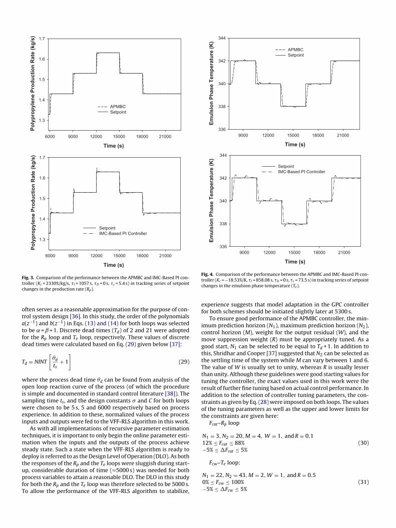

Time (s)

2100018000150001200090006000

Po

lyp

rop

yle

ne P

rod

ucti

on

Rate

(kg

/s)

1.3

1.4

1.5

1.6

1.7

APMBC

Setpoint

Time (s)

2100018000150001200090006000

Po

lyp

rop

yle

ne P

rod

ucti

on

Rate

(kg

/s)

1.3

1.4

1.5

1.6

1.7

Setpoint

IMC-Based PI Controller

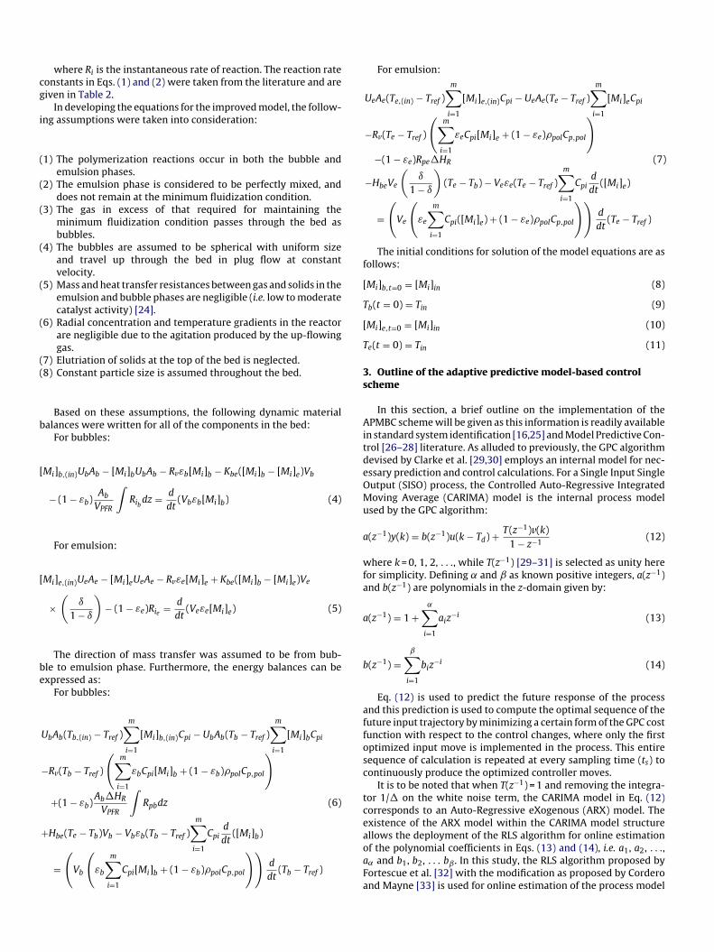
Fig. 3. Comparison of the performance between the APMBC and IMC-Based PI con-tc

otatfd

T

woiswei

tmsdtupfT

Time (s)

210001800015000120009000

Em

uls

ion

Ph

ase T

em

pera

ture

(K

)

336

338

340

342

344

APMBC

Setpoint

Time (s)

210001800015000120009000

Em

uls

ion

Ph

ase T

em

pera

ture

(K

)

336

338

340

342

344

Setpoint

IMC-Based PI Controller

Fig. 4. Comparison of the performance between the APMBC and IMC-Based PI con-

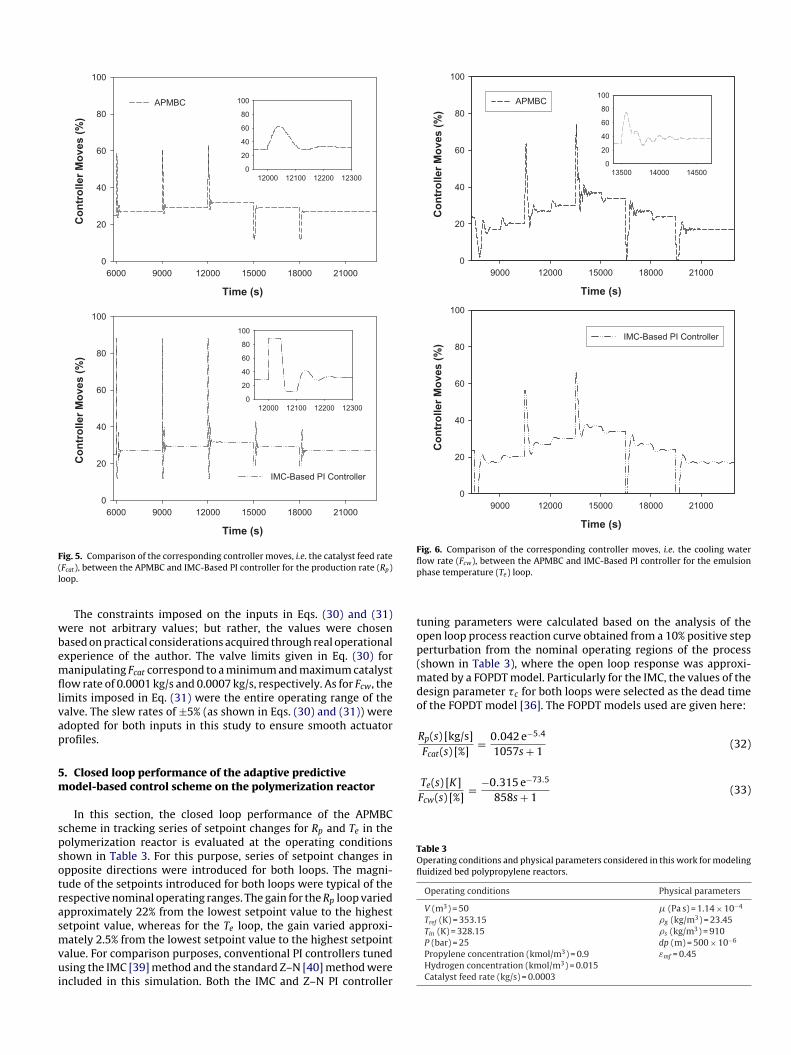
roller (Kc = 2330%/kg/s, I = 1057 s, D = 0 s, c = 5.4 s) in tracking series of setpointhanges in the production rate (Rp).

ften serves as a reasonable approximation for the purpose of con-rol system design [36]. In this study, the order of the polynomials(z−1) and b(z−1) in Eqs. (13) and (14) for both loops was selectedo be = = 1. Discrete dead times (Td) of 2 and 21 were adoptedor the Rp loop and Te loop, respectively. These values of discreteead times were calculated based on Eq. (29) given below [37]:

d = NINT

[�d

ts+ 1

](29)

here the process dead time �d can be found from analysis of thepen loop reaction curve of the process (of which the procedures simple and documented in standard control literature [38]). Theampling time ts, and the design constants � and C for both loopsere chosen to be 5 s, 5 and 6000 respectively based on process

xperience. In addition to these, normalized values of the processnputs and outputs were fed to the VFF-RLS algorithm in this work.

As with all implementations of recursive parameter estimationechniques, it is important to only begin the online parameter esti-

ation when the inputs and the outputs of the process achieveteady state. Such a state when the VFF-RLS algorithm is ready toeploy is referred to as the Design Level of Operation (DLO). As bothhe responses of the Rp and the Te loops were sluggish during start-p, considerable duration of time (≈5000 s) was needed for both

rocess variables to attain a reasonable DLO. The DLO in this studyor both the Rp and the Te loop was therefore selected to be 5000 s.o allow the performance of the VFF-RLS algorithm to stabilize,

troller (Kc = −18.53%/K, I = 858.08 s, D = 0 s, c = 73.5 s) in tracking series of setpointchanges in the emulsion phase temperature (Te).

experience suggests that model adaptation in the GPC controllerfor both schemes should be initiated slightly later at 5300 s.

To ensure good performance of the APMBC controller, the min-imum prediction horizon (N1), maximum prediction horizon (N2),control horizon (M), weight for the output residual (W), and themove suppression weight (R) must be appropriately tuned. As agood start, N1 can be selected to be equal to Td + 1. In addition tothis, Shridhar and Cooper [37] suggested that N2 can be selected asthe settling time of the system while M can vary between 1 and 6.The value of W is usually set to unity, whereas R is usually lesserthan unity. Although these guidelines were good starting values fortuning the controller, the exact values used in this work were theresult of further fine tuning based on actual control performance. Inaddition to the selection of controller tuning parameters, the con-straints as given by Eq. (28) were imposed on both loops. The valuesof the tuning parameters as well as the upper and lower limits forthe constraints are given here:

Fcat–Rp loop

N1 = 3, N2 = 20, M = 4, W = 1, and R = 0.112% ≤ Fcat ≤ 88%−5% ≤ �Fcat ≤ 5%

(30)

Fcw–Te loop:

N1 = 22, N2 = 43, M = 2, W = 1, and R = 0.50% ≤ Fcw ≤ 100%−5% ≤ �Fcw ≤ 5%

(31)

Time (s)

2100018000150001200090006000

Co

ntr

oller

Mo

ves (

%)

0

20

40

60

80

100

APMBC

12300122001210012000

0

20

40

60

80

100

Time (s)

2100018000150001200090006000

Co

ntr

oller

Mo

ves (

%)

0

20

40

60

80

100

IMC-Based PI Controller

12300122001210012000

0

20

40

60

80

100

F(l

wbemfllvap

5m

spsotrasmvui

Time (s)

210001800015000120009000

Co

ntr

oller

Mo

ves (

%)

0

20

40

60

80

100

APMBC

145001400013500

0

20

40

60

80

100

Time (s)

210001800015000120009000

Co

ntr

oller

Mo

ves (

%)

0

20

40

60

80

100

IMC-Based PI Controller

Fig. 6. Comparison of the corresponding controller moves, i.e. the cooling waterflow rate (Fcw), between the APMBC and IMC-Based PI controller for the emulsion

Fcw(s) [%]=

858s + 1(33)

Table 3Operating conditions and physical parameters considered in this work for modelingfluidized bed polypropylene reactors.

Operating conditions Physical parameters

V (m3) = 50 � (Pa s) = 1.14 × 10−4

Tref (K) = 353.15 �g (kg/m3) = 23.45Tin (K) = 328.15 �s (kg/m3) = 910

ig. 5. Comparison of the corresponding controller moves, i.e. the catalyst feed rateFcat), between the APMBC and IMC-Based PI controller for the production rate (Rp)oop.

The constraints imposed on the inputs in Eqs. (30) and (31)ere not arbitrary values; but rather, the values were chosen

ased on practical considerations acquired through real operationalxperience of the author. The valve limits given in Eq. (30) foranipulating Fcat correspond to a minimum and maximum catalyst

ow rate of 0.0001 kg/s and 0.0007 kg/s, respectively. As for Fcw, theimits imposed in Eq. (31) were the entire operating range of thealve. The slew rates of ±5% (as shown in Eqs. (30) and (31)) weredopted for both inputs in this study to ensure smooth actuatorrofiles.

. Closed loop performance of the adaptive predictiveodel-based control scheme on the polymerization reactor

In this section, the closed loop performance of the APMBCcheme in tracking series of setpoint changes for Rp and Te in theolymerization reactor is evaluated at the operating conditionshown in Table 3. For this purpose, series of setpoint changes inpposite directions were introduced for both loops. The magni-ude of the setpoints introduced for both loops were typical of theespective nominal operating ranges. The gain for the Rp loop variedpproximately 22% from the lowest setpoint value to the highestetpoint value, whereas for the Te loop, the gain varied approxi-

ately 2.5% from the lowest setpoint value to the highest setpoint

alue. For comparison purposes, conventional PI controllers tunedsing the IMC [39] method and the standard Z–N [40] method were

ncluded in this simulation. Both the IMC and Z–N PI controller

phase temperature (Te) loop.

tuning parameters were calculated based on the analysis of theopen loop process reaction curve obtained from a 10% positive stepperturbation from the nominal operating regions of the process(shown in Table 3), where the open loop response was approxi-mated by a FOPDT model. Particularly for the IMC, the values of thedesign parameter c for both loops were selected as the dead timeof the FOPDT model [36]. The FOPDT models used are given here:

Rp(s) [kg/s]Fcat(s) [%]

= 0.042 e−5.4

1057s + 1(32)

Te(s) [K] −0.315 e−73.5

P (bar) = 25 dp (m) = 500 × 10−6

Propylene concentration (kmol/m3) = 0.9 εmf = 0.45Hydrogen concentration (kmol/m3) = 0.015Catalyst feed rate (kg/s) = 0.0003

Time (s)

2100018000150001200090006000

Pro

du

cti

on

Ra

te

Pre

dic

tio

n E

rro

r (k

g/s

)

-0.004

-0.002

0.000

0.002

Em

uls

ion

Ph

as

e T

em

pe

ratu

re

Pre

dic

tio

n E

rro

r (K

)

-0.045

0.000

0.045

0.090

Rp loop

Te loop

Fp

s

cff

Fcrs

Time (s)

29000280002700026000250002400023000Po

lyp

rop

yle

ne P

rod

ucti

on

Rate

(kg

/s)

1.420

1.425

1.430

1.435

1.440

IMC-Based PI Controller

APMBC

Ph

ase T

em

pera

ture

(K

)341.8

342.0

342.2

342.4IMC-Based PI Controller

APMBC

ig. 7. Prediction errors for the production rate (Rp) and the emulsion phase tem-erature (Te) loops during closed loop simulations.

Also given here are the Fcw–Rp and Fcat–Te relationships for theake of completeness:

Rp(s) [kg/s]Fcw(s) [%]

= 0.0024 e−100

1819s + 1(34)

Te(s) [K]Fcat(s) [%]

= 0.45 e−95.5

1755s + 1(35)

From the simulation results, the Z–N PI controller producedhaotic closed loop transients and non-realizable controller movesor both the Rp and Te loops. Hence, it shall be more meaning-ul to restrict the following discussion to the APMBC and IMC PI

Time (s)

29000280002700026000250002400023000Po

lyp

rop

yle

ne P

rod

ucti

on

Rate

(kg

/s)

1.420

1.425

1.430

1.435

1.440

IMC-Based PI Controller

APMBC

Time (s)

29000280002700026000250002400023000

Em

uls

ion

Ph

ase T

em

pera

ture

(K

)

341.6

341.8

342.0

342.2

342.4IMC-Based PI Controller

APMBC

ig. 8. Comparison of the performance between the APMBC and the IMC-Based PIontroller in rejecting the effect of superficial gas velocity (U0) on the productionate (Rp) and the emulsion phase temperature (Te) loops. A 10% increment in theuperficial gas velocity was introduced at time = 25,000 s.

Time (s)

29000280002700026000250002400023000

Em

uls

ion

341.6

Fig. 9. Comparison of the performance between the APMBC and the IMC-Based PI

controller in rejecting the effect of hydrogen concentration (CH) on the produc-tion rate (Rp) and the emulsion phase temperature (Te) loops. A 10% increment inhydrogen flow rate was introduced at time = 25,000 s.

controllers only. Figs. 3–6 show the performance of the APMBC ascompared to the IMC PI controller in tracking series of setpointchanges for the Rp and the Te loops as well as the correspond-ing controller moves. The shortcomings exhibited by the Z–N PIcontroller (not shown), were not observed for the APMBC and theIMC-Based PI controller. In general, both the APMBC and the IMC-Based PI controller were able to track the changes in the setpointfor both loops. However, upon further scrutiny, the quality of thesetpoint tracking as demonstrated by the APMBC was superior tothe IMC-Based PI controller in terms of the ability to attain min-imal overshoot and minimize the effect of loop interactions. Asopposed to the APMBC where the responses for both loops showednegligible overshoot and minimal effect of loop interactions, theIMC-Based PI controller produced overshoots for both the Rp andthe Te loops, in addition to the obvious effect of loop interactionsfor the Te loop. Moreover, as depicted in Fig. 5, the IMC-Based PIcontroller exhibited sudden ‘spikes’ in the controller moves profilefor the Rp loop. Such sudden aggressive controller moves (i.e. largeslew rates), although infrequent, should be avoided where possibleduring practical implementations. The APMBC, on the other hand,was able to not only produce controller moves which were wellwithin the specified input constraints for both loops, but also thecontroller moves produced were non-aggressive and sufficientlysmooth for practical implementations. These were attributed tothe ability of the APMBC to handle constraints in the inputs and

the slew rates, of which conventional PI controllers are unable toachieve. To summarize, Table 4 shows the integral absolute error(IAE) for all three controllers in tracking series of setpoint changesfor both loops. The values of the IAE calculated for both loops were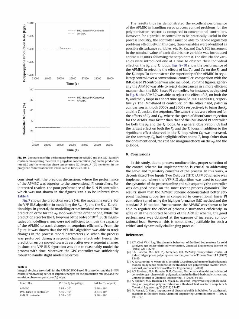

Time (s)

29000280002700026000250002400023000

Po

lyp

rop

yle

ne P

rod

ucti

on

Rate

(kg

/s)

1.420

1.425

1.430

1.435

1.440

IMC-Based PI Controller

APMBC

Time (s)

29000280002700026000250002400023000

Co

ntr

oller

Mo

ves (

%)

0

20

40

60

80

100

IMC-Based PI Controller

APMBC

Fig. 10. Comparison of the performance between the APMBC and the IMC-Based PIcontroller in rejecting the effect of propylene concentration (CM) on the productionrp

coiwT

ttpptoficwpIpr

TIce

ate (Rp) and the emulsion phase temperature (Te) loops. A 10% increment in theropylene concentration was introduced at time = 25,000 s.

onsistent with the previous discussions, where the performancef the APMBC was superior to the conventional PI controllers. Fornterested readers, the poor performance of the Z–N PI controller,

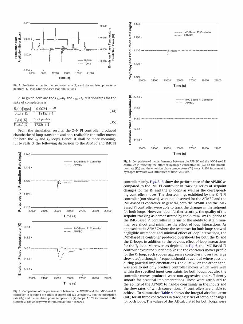
hich was not shown in the figures, can also be inferred fromable 4.

Fig. 7 shows the prediction errors (viz. the modelling errors) forhe VFF-RLS algorithm in modelling the Fcat–Rp and the Fcw–Te rela-ionships. In general, the modelling errors involved were small. Therediction error for the Rp loop was of the order of one, while therediction error for the Te loop was of the order of 10−3. Such magni-udes of modelling errors were not sufficient to impair the capacityf the APMBC to track changes in setpoints efficiently. From thegure, it was shown that the VFF-RLS algorithm was able to trackhanges in the process model parameters (i.e. when the processas perturbed during a setpoint change) effectively. Hence, therediction errors moved towards zero after every setpoint change.

n short, the VFF-RLS algorithm was able to reasonably model therocess with time. Moreover, the GPC controller was sufficientlyobust to handle slight modelling errors.

able 4ntegral absolute error (IAE) for the APMBC, IMC-Based PI controller, and the Z–N PIontroller in tracking series of setpoint changes for the production rate (Rp) and themulsion phase temperature (Te) loops.

Controller IAE for Rp loop (kg/s) IAE for Te loop (K)

APMBC 3.84 × 104 2.46 × 103

IMC-Based PI controller 4.49 × 104 2.63 × 103

Z–N PI controller 1.32 × 106 5.56 × 103

The results thus far demonstrated the excellent performanceof the APMBC in handling servo process control problems for thepolymerization reactor as compared to conventional controllers.However, for a particular controller to be practically useful in theprocess industry, the controller must be able to handle regulatoryproblems effectively. In this case, three variables were identified aspossible disturbance variables, viz. U0, CH, and CM. A 10% incrementin the nominal value of each disturbance variable was introducedat time = 25,000 s, following the setpoint test. The disturbance vari-ables were introduced one at a time to observe their individualeffect on the Rp and Te loops. Figs. 8–10 show the performance ofthe APMBC in rejecting the effects of U0, CH, and CM on the Rp andthe Te loops. To demonstrate the superiority of the APMBC in regu-latory control over a conventional controller, comparison with theIMC-Based PI controller was also included. From the figures, gener-ally the APMBC was able to reject disturbances in a more efficientmanner than the IMC-Based PI controller. For instance, as depictedin Fig. 8, the APMBC was able to reject the effect of U0 on both theRp and the Te loops in a short time span (i.e. 300 s and 600 s, respec-tively). The IMC-Based PI controller, on the other hand, paled incomparison as it took 3000 s and 3500 s respectively to bring the Rp

and the Te back to the setpoints. The same trends were observed forthe effects of CH and CM, where the speed of disturbance rejectionfor the APMBC was faster than that of the IMC-Based PI controllerfor both the Rp and the Te loops. As a general observation, U0 hadthe largest effect on both the Rp and the Te loops in addition to thesignificant effect observed in the Te loop when CM was increased.On the contrary, CH had negligible effect on the Te loop. Other thanthe ones mentioned, the rest had marginal effects on the Rp and theTe loops.

6. Conclusions

In this study, due to process nonlinearities, proper selection ofthe control scheme for implementation is crucial to addressingthe servo and regulatory concerns of the process. In this work, adecentralized Two Inputs Two Outputs (TITO) APMBC scheme wasimplemented, where the VFF-RLS algorithm was used to capturethe dynamics of the process online and subsequently the controllerwas designed based on the most recent process dynamics. Theresults show that the APMBC scheme demonstrated better set-point tracking properties as compared to conventional linear PIcontrollers tuned using the high performance IMC method and thestandard Z–N method. Furthermore, the APMBC was shown to beable to regulate the effect of process disturbances efficiently. Inspite of all the reported benefits of the APMBC scheme, the goodperformance was obtained at the expense of increased compu-tational load. However, this is nonetheless justifiable for such acritical and dynamically challenging process.

References

[1] K.Y. Choi, W.H. Ray, The dynamic behaviour of fluidized bed reactors for solidcatalysed gas phase olefin polymerization, Chemical Engineering Science 40(1985) 2261–2279.

[2] S.A. Dadebo, M.L. Bell, P.J. McLellan, K.B. McAuley, Temperature control ofindustrial gas phase polyethylene reactors, Journal of Process Control 7 (1997)83–95.

[3] A. Sarvaramini, N. Mostoufi, R. Sotudeh-Gharebagh, Influence of hydrodynamicmodels on dynamic response of the fluidized bed polyethylene reactor, Inter-national Journal of Chemical Reactor Engineering 6 (2008).

[4] A.S. Ibrehem, M.A. Hussain, N.M. Ghasem, Mathematical model and advancedcontrol for gas-phase olefin polymerization in fluidized-bed catalytic reactors,Chinese Journal of Chemical Engineering 16 (2008) 84–89.

[5] A. Shamiri, M.A. Hussain, F.S. Mjalli, N. Mostoufi, Improved single phase mod-

eling of propylene polymerization in a fluidized bed reactor, Computers &Chemical Engineering 36 (2012) 35–47.

[6] M. Aoyagi, D. Kunii, Importance of dispersed solids in bubbles for exothermicreactions in fluidized beds, Chemical Engineering Communications 1 (1974)191–197.

[

[

[

[

[

[

[

[

[

[

[

[

[

[

[

[

[

[

[[

[

[

[

[

[

[

[

[

[

[

[

[

[

[

[7] H. Cui, N. Mostoufi, J. Chaouki, Characterization of dynamic gas–solid distribu-tion in fluidized beds, Chemical Engineering Journal 79 (2000) 133–143.

[8] H. Cui, N. Mostoufi, J. Chaouki, Gas and solids between dynamic bubble andemulsion in gas-fluidized beds, Powder Technology 120 (2001) 12–20.

[9] A.R. Abrahamsen, D. Geldart, Behaviour of gas-fluidized beds of fine powderspart: II. Voidage of the dense phase in bubbling beds, Powder Technology 26(1980) 47–55.

10] K.B. McAuley, J.F. Macgregor, Nonlinear product property control in industrialgas-phase polyethylene reactors, AIChE Journal 39 (1993) 855–866.

11] B.W. Bequette, Nonlinear control of chemical processes: a review, Industrial &Engineering Chemistry Research 30 (1991) 1391–1413.

12] R. Di Marco, D. Semino, A. Brambilla, From linear to nonlinear model pre-dictive control: comparison of different algorithms, Industrial & EngineeringChemistry Research 36 (1997) 1708–1716.

13] D.E. Seborg, T.F. Edgar, S.L. Shah, Adaptive control strategies for process control:a survey, AIChE Journal 32 (1986) 881–913.

14] S.L. Shah, W.R. Cluett, Recursive least squares based estimation schemes forself-tuning control, Canadian Journal of Chemical Engineering 69 (1991) 89–96.

15] K.J. Åström, Theory and applications of adaptive control – a survey, Automatica19 (1983) 471–486.

16] L. Ljung, T. Söderstöm, Theory and Practice of Recursive Identification, MITPress, Massachusettes, 1983.

17] D.T. Ahlberg, I. Cheyne, Adaptive control of a polymerization reactor AIChESymposium Series, 1976, p. 221.

18] K.M. Kwalik, F.J. Schork, Adaptive control of a continuous polymerization reac-tor, in: Proceedings of the American Control Conference, Boston, 1985, pp.872–877.

19] H.-J. Rho, Y.-J. Huh, H.-K. Rhee, Application of adaptive model-predictive con-trol to a batch MMA polymerization reactor, Chemical Engineering Science 53(1998) 3729–3739.

20] S.A. Mendoza-Bustos, A. Penlidis, W.R. Cluett, Adaptive control of conversion ina simulated solution polymerization continuous stirred tank reactor, Industrial& Engineering Chemistry Research 29 (1990) 82–89.

21] G.G. Elicabe, G.R. Meira, Estimation, Control in polymerization reactors. Areview, Polymer Engineering and Science 28 (1988) 121–135.

22] A. Shamiri, M.A. Hussain, F.S. Mjalli, N. Mostoufi, Kinetic modeling of propylenehomopolymerization in a gas-phase fluidized-bed reactor, Chemical Engineer-ing Journal 161 (2010) 240–249.

23] A. Shamiri, M. Azlan Hussain, F. Sabri Mjalli, N. Mostoufi, M. Saleh Shafeeyan,Dynamic modeling of gas phase propylene homopolymerization in fluidized

bed reactors, Chemical Engineering Science 66 (2011) 1189–1199.

24] S. Floyd, K.Y. Choi, T.W. Taylor, W.H. Ray, Polymerization of olefins throughheterogeneous catalysis: III. Polymer particle modelling with an analysis ofintraparticle heat and mass transfer effects, Journal of Applied Polymer Science32 (1986) 2935–2960.

[

[

25] L. Ljung, System Identification: Theory for the User, Prentice Hall, New Jersey,1987.

26] E.F. Camacho, C. Bordons, Model Predictive Control, Springer-Verlag, Berlin,1999.

27] J.M. Maciejowski, Predictive Control with Constraints, Prentice Hall, EnglewoodCliffs, New Jersey, 2002.

28] J.A. Rossiter, Model-Based Predictive Control, CRC Press, Boca Raton, FL, 2004.29] D.W. Clarke, C. Mohtadi, P.S. Tuffs, Generalized predictive control – Part I. The

basic algorithm, Automatica 23 (1987) 137–148.30] D.W. Clarke, C. Mohtadi, P.S. Tuffs, Generalized predictive control – Part II.

Extensions and interpretations, Automatica 23 (1987) 149–160.31] T.-W. Yoon, D.W. Clarke, Observer design in receding-horizon predictive con-

trol, International Journal of Control 61 (1995) 171–191.32] T.R. Fortescue, L.S. Kershenbaum, B.E. Ydstie, Implementation of self-tuning

regulators with variable forgetting factors, Automatica 17 (1981) 831–835.33] A.O. Cordero, D.Q. Mayne, Deterministic convergence of a self-tuning regu-

lator with variable forgetting factor, IEEE Proceedings D: Control Theory andApplications 128 (1981) 19–23.

34] G.J. Bierman, Measurement updating using the U-D factorization, Automatica12 (1976) 375–382.

35] J. Mikles, M. Fikar, Process Modelling, Identification and Control, Springer-Verlag, Berlin, 2007.

36] G.H. Cohen, G.A. Coon, Theoretical Considerations of Retarded Control, Trans-actions of the ASME 75 (1953) 827.

37] R. Shridhar, D.J. Cooper, A tuning strategy for unconstrained SISO model predic-tive control, Industrial and Engineering Chemistry Research 36 (1997) 729–746.

38] D.E. Seborg, T.F. Edgar, D.A. Mellichamp, Process dynamics and control, seconded., John Wiley & Sons, Inc., New Jersey, 2004.

39] I.L. Chien, P.S. Fruehauf, Consider IMC tuning to improve controller perfor-mance, Chemical Engineering Progress 86 (1990) 33–41.

40] J.G. Ziegler, N.B. Nichols, Optimum settings for automatic controllers, Transac-tions of the ASME 64 (1942) 759–768.

41] A. Lucas, J. Arnaldos, J. Casal, L. Puigjaner, Improved equation for the calculationof minimum fluidization velocity, Industrial & Engineering Chemistry ProcessDesign and Development 25 (1986) 426–429.

42] D. Kunii, O. Levenspiel, Fluidization Engineering, second ed., Butterworth-Heinmann, Boston, MA, 1991.

43] N. Mostoufi, H. Cui, J. Chaouki, A comparison of two- and single-phase mod-els for fluidized-bed reactors, Industrial & Engineering Chemistry Research 40(2001) 5526–5532.

44] K. Hilligardt, J. Werther, Local bubble gas hold-up and expansion of gas/solidfluidized beds, German Chemical Engineering 9 (1986) 215–221.

45] Z.-H. Luo, P.-L. Su, D.-P. Shi, Z.-W. Zheng, Steady-state and dynamic model-ing of commercial bulk polypropylene process of Hypol technology, ChemicalEngineering Journal 149 (2009) 370–382.