CONTROL OF HEIGHT GROWTH IN HYDRAULIC FRACTURING

By

Kizza Francis Xavier

Submitted in Partial Fulfillment of the Requirements for the Degree of Master of Engineering

At

Dalhousie University

Halifax, Nova Scotia

August 2013

©Kizza Francis Xavier 2013

i

DALHOUSIE UNIVERSITY

PETROLEUM ENGINEERING

The undersigned hereby certifies that he has read and recommended to the Faculty of Graduate

Studies for acceptance a thesis entitled ―CONTROL OF FRACTURE HEIGHT GROWTH

IN HYDRAULIC FRACTURING‖ by Kizza Francis Xavier in partial fulfillment of the

requirements for the degree of Master of Engineering in Petroleum Engineering.

Date: August 2013

Supervisor: Dr. Dmitry Garagash ………………………………

Reader: Dr. Michael Pegg……………………………...

ii

DALHOUISE UNIVERSITY

DATE: AUGUST 2013

TITLE: CONTROL OF HEIGHT GROWTH IN HYDRAULIC FRACTURING

DEPARTMENT: PROCESS ENGINEERING AND APPLIED SCIENCE (PEAS)

DEGREE: MASTER OF ENGINEERING (M.Eng)

CONVOCATION: OCTOBER 2013

Permission is herewith granted to Dalhousie University to circulate and to have copied for non-

commercial purposes, at its discretion, the above title upon the request of individuals or

institutions

……………………………………..

Signature of Author

The author reserves the other publication rights, and neither the thesis nor extensive extracts

from it may be printed or otherwise reproduced without the author‘s written permission.

The author attests that permission has been obtained for the use of any copyrighted material

appearing in the thesis (other than the brief excerpts requiring only proper acknowledgement in

scholarly writing) and that all such use is clearly acknowledged.

iii

DEDICATION

I dedicate this work to my family; for believing in me and sacrificing a lot so as I can attain

quality and valuable education at Dalhousie University.

iv

TABLE OF CONTENTS

List of figures…………………………………………………………………………………….v

Nomenclature……………………………………………………………………………………vii

Abstract………………………………………………………………………………………….viii

Acknowledgements………………………………………………………………………………ix

Chapter one: Introduction to hydraulic fracturing

1.0 Definition………………………………………………………………….1

1.1 Reasons for hydraulic fracturing………………………………………..…2

1.2 History…………………………………………………………………….2

1.3 Equipment used…………………………………………………………....3

1.4 The process………………………………………………………………..6

Chapter two: Formation evaluation

2.0 Introduction………………………………………………………………………9

2.1 Geology…………………………………………………………………………..9

2.2 Coring……………………………………………………………………………16

2.3 Logging…………………………………………………………………………..19

2.4 Well testing………………………………………………………………………21

Chapter three: Understanding rock mechanics

3.0 Introduction………………………………………………………………………23

3.1 In-situ stress……………………………………………………………………..24

3.2 Rock properties………………………………………………………………….29

Chapter four: Hydraulic Fracture Modeling

4.0 Introduction………………………………………………………………………31

4.1 Two dimensional fracture propagation model…………………………………...31

4.2 Three dimensional fracture propagation model………………………………….40

Chapter five: Fracture Height control

5.0 Introduction………………………………………………………………………47

5.1 Determining fracture height……………………………………………………...47

5.2 Fracture height control…………………………………………………………...53

Chapter six: Case study…………………………………………………………………………..66

6.1 Argument for……………………………………………………………………..67

6.2 Argument against…………………………………………………………………70

6.3 Conclusion………………………………………………………………………..76

References………………………………………………………………………………………..78

v

LIST OF FIGURES

Figure 1.1: Casing and cementing of a horizontally drilled well………………………………….7

Figure 1.2: Hydraulic fracturing process………………………………………………………….8

Figure 2.1: Detrital clays…………………………………………………………………………11

Figure 2.2 Authigenic clays……………………………………………………………………..11

Figure 2.3 Authigenic Kaolinite…………………………………………………………………12

Figure 2.4 Authigenic chlorite…………………………………………………………………...13

Figure 2.5 Authigenic Illite………………………………………………………………………13

Figure 2.6 Pore throat with overgrowth………………………………………………………….14

Figure 2.7 Whole core samples…………………………………………………………………..16

Figure 2.8 Side wall cores………………………………………………………………………..17

Figure 3.1 Hydraulic fracture test used to measure in-situ stress………………………………..27

Figure 3.2 Step rate/Flow back test………………………………………………………………28

Figure 4.1 PKN fracture model…………………………………………………………………..34

Figure 4.2 KGD fracture model………………………………………………………………….38

Figure 4.3 Planar 3D representation in the form of squares……………………………………..43

Figure 4.4 Fixed grid solution……………………………………………………………………44

Figure 5.1 Impression packer application ……………………………………………………….50

Figure 5.2 BHTV………………………………………………………………………………...51

Figure 5.3 Downhole television………………………………………………………………….52

vi

Figure 5.4 Fracture height variation with injection rate and total volume fluid injected………..57

Figure 5.5 Influence of the choice of the fracturing fluid on the resulting fracture height……...59

Figure 5.6 Proppant placement…………………………………………………………………..61

Figure 5.7 Termination of fracture near fault……………………………………………………63

Figure 5.8 Offset of hydraulic fracture at the natural fracture…………………………………...64

Figure 5.9 Fracture kinking, offsetting and turning at the bedding planes………………………64

Figure 6.0 Visualization of fracture treatment in a jointed formation…………………………...65

Figure 6.1 Illustration of the possible forms of casing leaks…………………………………….67

Figure 6.2 Map of drilling operations and well water sampling locations in Pennsylvania and

New York………………………………………………………………………………………..69

Figure 6.3 Plot relating the methane concentration in water relative to the distance to the nearest

gas well…………………………………………………………………………………………..70

Figure 6.4 Underground water aquifer position relative to fracture height growth for six shale

basins in North America………………………………………………………………………....71

Figure 6.5 Map showing the location and the position of water aquifers relative to the shale

payzones of the different shale plays in the United States……………………………………….72

Figure 6.6 Fracture heights in the Barnett shale relative to the aquifers………………………...73

Figure 6.7 Fracture heights in the Woodford shale relative to the aquifers……………………...74

Figure 6.8 Fracture heights in the Marcellus shale relative to the aquifers……………………...75

Figure 6.8 General positioning of the hydraulic fractures relative to the nearest aquifer……….77

vii

NOMENCLATURE

𝛥𝑡𝑠 – shear wave travel time (s)

𝛥𝑡𝑐 – compressional wave travel time (s)

𝜍𝑒 - Effective stress (psi)

𝜍- Compressive stress (psi)

𝑝𝑝- Pore pressure (psi)

𝜍𝑣- Overburden stress (psi)

𝜌 – Density (lb/ft3)

𝑧 – Depth (ft)

𝑔 – Gravitational acceleration (ft/s2)

Pnet; Net pressure = Pressure in crack – Stress against which it opens (psi)

qi - Injection rate (ft3/s)

μ – viscosity (cp)

v - Poisson‘s ratio

E - Young‘s modulus (lb/ft2 or psi)

uL - Leakoff velocity (ft2)

CL - Leakoff coefficient (ft/s1/2

)

t – Time (s)

texp - Time at which point uL was exposed (s)

𝑡𝐷 – Dimensionless time

viii

ABSTRACT

The application of hydraulic fracturing in the production of hydrocarbons from ‗tight‘

impermeable formations has been discredited by environmentalists with an analogy that

hydraulic fracturing leads to water aquifer contamination with the generated hydraulic fractures

acting as links to the aquifers. Hence, this report reviews the history and the basics of hydraulic

fracturing. The ways to determine if the formation requires hydraulic fracturing application are

also explained. Fracture height modeling and rock mechanics principles in relation to fracture

height growth are also explained. Some of the ways used for fracture height containment are also

clearly elaborated. Then at the end there is an investigative case study to determine if really

hydraulic fracturing causes underground water contamination through the upward migration of

hydrocarbons via the generated fractures to the aquifers. After the careful analysis of the case

study I conclude that aquifer contamination with the generated fractures acting as conduits is

practically impossible due to the significant vertical distance between the payzone and the

aquifers.

ix

ACKNOWLEDGEMENTS

I sincerely appreciate Dr. Dmitry Garagash for his supervisory role well played during the

concept inception and compilation of this report.

On a special note, I thank my dear family; mum, dad, brothers and sisters for their support

throughout my academic life here at Dalhousie University and in my life in general.

And last but not least, I also give praise and thanks to the Almighty God for the wisdom and

good health throughout my life and in the period of the project compilation to be specific.

1

CHAPTER 1

INTRODUCTION TO HYDRAULIC FRACTURING

1.0: DEFINITION

Hydraulic fracturing is a process by which a fluid, proppant and additives are pumped into tight

formations like shale at high pressures creating cracks or opening wider already existing ones

enabling easier flow of hydro carbons into the well bore and finally to the surface facilities.

Hydraulic fracturing commonly referred to now days as ―fracking‖ is mainly used in the

production of hydrocarbons. The proppant in the hydraulic fracturing fluid ensures that once the

cracks are created, they do not close instantly hence enabling the flow of the hydrocarbon from

the tight formation over a period of time. The additives consist of various types of chemicals and

each of the chemicals enhances as specific property of the fluid required for the success of the

hydraulic fracturing process.

However, much as hydraulic fracturing technology makes the production of natural gas from

impermeable formations possible, on several occasions it has been held responsible for the

underground water contamination among other environmental concerns which poses a great risk

to the biological life on earth whose livelihoods almost entirely depend on the availability of

clean or safe water.

Therefore with proper hydraulic fracturing modeling, fracture height growth can be controlled

from penetrating the cap rock which leads to leaking of hydrocarbons say methane plus other

naturally existing chemicals into water aquifers.

2

1.1: REASONS FOR HYDRAULIC FRACTURING

Some of the reasons for hydraulic fracturing are as follows;

Hydraulic fracturing is used to bypass well bore damage that affects productivity. Near well bore

damage is attributed to fines invasion of the formation during drilling and chemical

incompatibility between the drilling fluids and the formation of interest. This can be overcome

chemically by the use of matrix treatments or by hydraulic fracturing so as to reinstate the

conductivity between the well bore and the formation.

Hydraulic fracturing enables the creation of conductive hydrocarbon pathways into formation to

enhance productivity. From Darcy‘s law, hydraulic fracturing improves the permeability of the

formation, increases the fracture height and area coverage while elevating or sustaining the

reservoir pressure enhancing well productivity.

Also, hydraulic fracturing is used to adjust fluid flow within the formation. A carefully designed

fracturing job can lead to fewer wells for development of the reservoir which improves the

economics of the development. (Economides & Nolte, 2011)

1.2: HISTORY

The birth of the hydraulic fracturing technology is attributed to Stanolind Oil in 1949.

The roots of hydraulic fracturing are dated back in the 1860s where nitroglycerin was used to

penetrate formations to improve the hydrocarbon recovery.

Then in the 1930s, the idea of injecting acid into low permeable formations was devised so as to

improve the economic hydrocarbon recovery. The acid used at high pressures initiated fractures

3

which could not completely close due to the acid etching of the rock enhancing hydrocarbon

recovery.

All this information was analyzed by Floyd Farris an employee of Stanolind Oil by co-relating

and studying the relationship of well performance, formation breakdown, during well acidizing,

and water injection leading to the development of hydraulic fracturing technology concept.

The first documented hydraulic fracturing well stimulation was in the Hugoton gas field on

Kelpper Well 1 in Grant County Kansas in 1947 by Stanolind Oil whereby 1000 gallons of

napalm thickened gasoline was injected followed by 2000 gallons of gasoline as a gel breaker to

stimulate a gas producing limestone formation at 2400ft though it is on record that the well

performance did not improve due to lack of proppant. The mechanical equipment involved

consisted of a centrifugal pump for mixing the gasoline based napalm gelled fracturing fluid and

a duplex positive displacement piston pump for pumping fluid into the well. (Gidley et al, 1989)

In 1949 a patent for the hydraulic fracturing process was issued to Halliburton Oil Well

Cementing Company. (Montgomery & Smith, 2010)

1.3: EQUIPMENT USED

Fluids initially used for treatments were gelled crude and gelled kerosene. In 1952 refined and

crude oils were used because they were inexpensive and they had low viscosities. They required

high pump rates to transport the proppant due to their lower viscosities. The viscosity of the fluid

is one of the most important property considered during fluid selection because it influences the;

fracture width, net pressure, ability to carry and transport proppant and fluid loss. (Bunger et al,

2013) Other factors considered during fluid selection include; human safety, environmentally

safe, ability to break to a low viscosity to enable flow back, cost, compatibility with the

4

formation, controllable fluid loss, easy to mix and so on. In 1953 water was used as a fracturing

fluid and the corresponding gelling agents were developed. Surfactants were then incorporated to

control the formation of emulsions. Potassium chloride was also added to reduce the effect on

clays and water sensitive formation constituents. Also the advent of foams and alcohol addition

enhanced the use of the water as a fracturing fluid. In 1970s the use of metal based cross linking

agents to improve the viscosity of gelled water based fracturing fluids for higher temperature

wells was invented. Some of the fluid gelling agents include cellulose, guar, napalm, soaps,

sodium bicarbonate, surfactants and so on. Examples of cross linking agents are aluminum,

antimony, born, chromium and so on. (Montgomery & Smith, 2010)

The main types of fracturing fluid can be classified into water base, linear gels, crosslinked gels,

oil base and foams (PolyEmulsions). Water base fluids as the name suggests mainly consist of

water, a clay control agent and friction reducer. Compared to other fluids, water based fluids are

of a relatively lower cost, easier to mix and very easy to recycle and re-use. The main pit fall of

the water base fluid is the low viscosity of the water which leads to; narrow fracture width and

proppant transport is achieved by pumping at extremely high rates. Linear gels consist of water,

clay control agent, gelling agent and bactericide. Linear gels are low cost with better viscosity

properties. Linear gels lead to narrow fractures and they are not re-usable. Crosslinked gels

consist of water, clay control agent, gelling agent, bactericide and a crosslinker. The crosslinker

greatly improves the fluid viscosity improving proppant transport leading to wider fracture

widths. Oil based fluids are applied in formations that are not compatible with water based

fluids. Oil based fluids are a threat to personnel safety and the environment compared to other

fluids. Foams can be made up of nitrogen, carbon dioxide or a hydrocarbon. PolyEmulsions are

made by emulsifying hydrocarbon with water. Viscosity is controlled by varying the water and

5

hydro carbon composition ratio. Foam fluids are in general expensive and a safety hazard.

(Montgomery & Smith, 2010)

Also fluid additives like gelling agents, crosslinkers, breakers, fluid loss additives, bactericides,

surfactants, clay control additives etcetera added to the fracturing fluid for specific functions

like antifoaming, bacteria control, viscosity breakers, clay stabilizers, defoamers, demulsifying,

reduce friction, control ph, scale inhibition, temperature stabilizing and so on. (Veatch, 2008)

The first proppant to be used during fracture treatment was screened river sand. With time

depending on the nature of the fracture treatment other proppants were developed like plastic

pellets, steel shot, Indian glass beads, aluminum pellets, high strength glass beads, rounded nut

shells, resin coated sands, sintered bauxite, fused zirconium and so on.

Pumps are used during fracturing treatment so as to pump the fracturing fluid and its contents

into the formation of interest. Blending equipment is also used so as to mix the various contents

of the fracturing fluid in their right proportions. Storage vessels/tanks are also used for the

storage of proppant in large quantities. Most of the fracturing field equipment is provided by the

oil service companies and they are always developing new and better equipment so as to better

the process.

6

1.4: THE PROCESS

Hydraulic fracturing is used in ‗tight‘ less permeable formations like deep shale, tight sands and

coal beds to produce hydro carbons most especially methane (natural) gas. Shale formations

consist of mud, silt, clay and organic matter which break down with time forming hydrocarbons.

However vertical drilling coupled with hydraulic fracturing limits the coverage of the payzone

and in the past decade horizontal drilling has been applied alongside hydraulic fracturing. This

improves the lateral/horizontal coverage of the formation increasing the production in due

process.

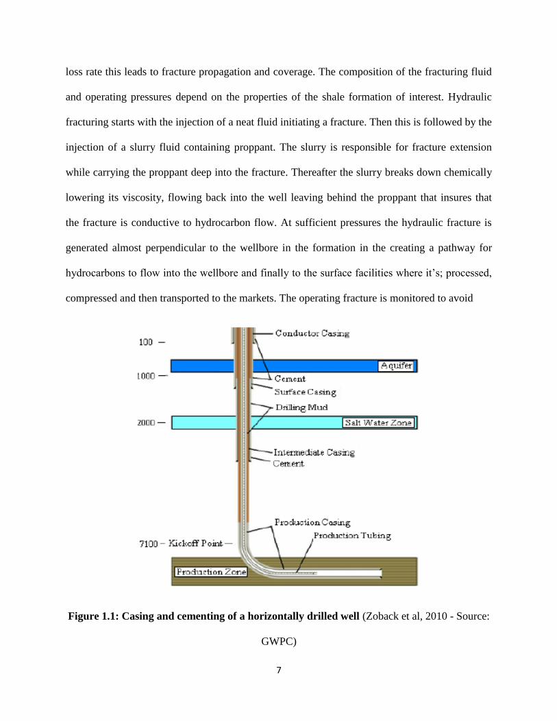
The process begins with drilling a considerable depth below the earth surface and a steel pipe

referred to as the conductor casing is installed into the vertical well bore so as stabilize the soil

around the well. Vertical drilling continues followed by the installation of the surface casing

which is installed below the shallow underground sources of drinking water as a requirement by

the legislation to protect aquifers. Thereafter cement is pumped down through the casing and up

through the wellbore annulus until it is filled and the casing is cemented in place. This is

followed by the installation of the blowout preventer commonly known as the BOP at the well

head to prevent any pressurized fluids encountered during drilling from jetting out from the

formation at the surface. Then vertical drilling continues and the intermediate casing is installed

at the appropriate depth to stabilize the deep wells and prevent the contamination of the produced

gas and the aquifers.

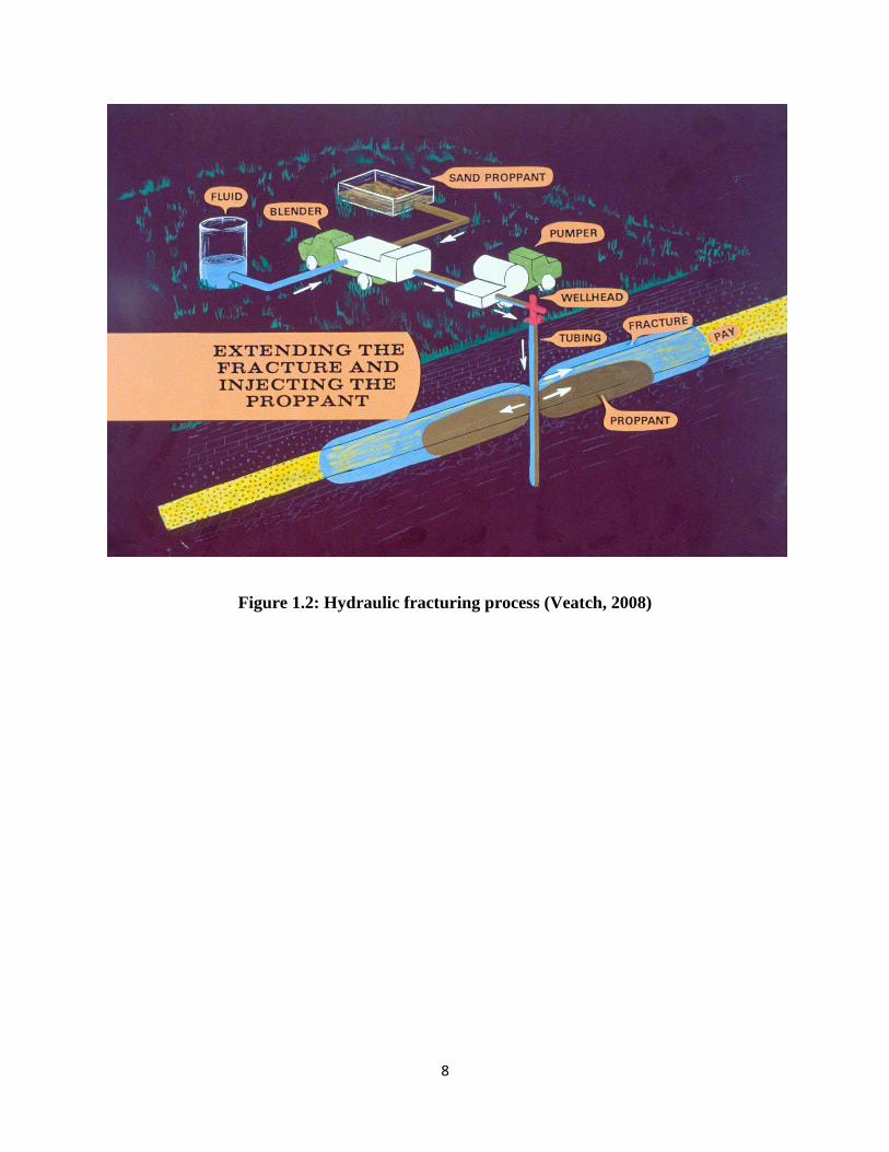
Hydraulic fracturing involves the pumping of the fracturing fluid into the formation pay zone at

extremes of pressure at a rate faster than the rate at which the fluid can escape into the formation

breaking the formation. If the hydraulic pump rate is maintained at a rate higher than the fluid

7

loss rate this leads to fracture propagation and coverage. The composition of the fracturing fluid

and operating pressures depend on the properties of the shale formation of interest. Hydraulic

fracturing starts with the injection of a neat fluid initiating a fracture. Then this is followed by the

injection of a slurry fluid containing proppant. The slurry is responsible for fracture extension

while carrying the proppant deep into the fracture. Thereafter the slurry breaks down chemically

lowering its viscosity, flowing back into the well leaving behind the proppant that insures that

the fracture is conductive to hydrocarbon flow. At sufficient pressures the hydraulic fracture is

generated almost perpendicular to the wellbore in the formation in the creating a pathway for

hydrocarbons to flow into the wellbore and finally to the surface facilities where it‘s; processed,

compressed and then transported to the markets. The operating fracture is monitored to avoid

Figure 1.1: Casing and cementing of a horizontally drilled well (Zoback et al, 2010 - Source:

GWPC)

8

Figure 1.2: Hydraulic fracturing process (Veatch, 2008)

9

CHAPTER 2

FORMATION EVALUATION

2.0: INTRODUCTION

Before the option of hydraulic fracturing, a form of reservoir stimulation is considered; the

formation has to meet the billing for its application since just like any other processes in the oil

and gas industry it is a very expensive process. This chapter reviews the criteria that have to be

met by the formation in question to consider the application of the hydraulic fracturing process.

The obvious reason for its application is in the low permeability formations so as to act as a

stimulation by creating fractures that are propped open by proppant enabling the easy flow of

hydro carbons from the reservoir to the well bore and then finally to the surface treatment

facilities. In this section; the geology of the formation, well logging, core analysis and well

testing are considered in depth so as to enable us better understand the formation that requires the

application of hydraulic fracturing.

Emphasis is on the pre hydraulic fracture formation

evaluation as regards to this chapter.

2.1 GEOLOGY

During the critical analysis of the geology, it is of great importance to determine the historical

form of sediment deposition in the area of interest which eventually leads to the formation of

either blanket or lenticular reservoirs. It is worth noting that in order to optimize hydraulic

fracturing treatment, the engineer must optimize the ratio of fracture length to drainage radius. 3

In blanket reservoirs, the ratio of the fracture length to the drainage radius is optimized.

Depending on the fracturing fluid flow rate the fracture length and drainage radius can be

optimized and at the same time determined. For the case of lenticular reservoirs, basing on

10

geologic experience the drainage radius is fixed. Then using the estimated drainage area, the

engineer determines the fracture length required to optimize production. (Jensen et al, 2003)

Henceforth, before any form of hydraulic fracturing, the reservoir engineer has to determine the

drainage radius and fracture length for the specific pay zone. In summary regional geologic

studies as well as local geologic studies of the reservoir of interest are obviously carried out prior

to any form fracture treatment. This is simplified by the thorough study and cross examination of

cross sections, structure maps, isopach maps of the formation of interest.

Also it is vital to know the type of lithology of the reservoir before fracture treatment, for

instance the lithology can be mainly sandstone or carbonate or any other type. Knowing the

lithology will enable you to determine the type of fracturing fluid to apply, for instance; for

predominantly sandstone reservoirs water based or oil based fracturing fluid is preferably used

and for predominantly carbonate reservoirs acid based fracturing fluid are commonly applied.

The choice of the specific fracturing fluid for a specific lithology is mainly due to the chemical

compatibility between the different entities since both contain different types of chemicals.

Therefore the type lithology of the reservoir greatly influences the fracturing fluid to use. Also

the thorough knowledge of the lithology enables the analysis of the well logs. Some formation

minerals influence the well log data which causes avoidable errors in the fracture treatment

planning stage. Under the same consideration the cementing material of the reservoir rock should

also be determined. The reservoir cementing material contains a variety of clay materials. For

instance if the carbonate cement is holding the reservoir soft rock, it is not advisable to use acid

based fluid for stimulation or else the reservoir will collapse into the well bore.

It is common knowledge that hydraulic fracturing is applied in low permeability reservoirs. Low

permeability is as the result of precipitates filling the pores of the formation and the precipitates

11

consist of mainly different kinds of clay material. Such clay is grouped into; detrital clays which

are due to physical processes after deposition or biogenic processes after deposition and

authigenic clays which are due to the direct precipitation from solution or regeneration of detrital

clays. (Gidley et al, 1989)

Figure 2.1 Detrital clays (Jensen et al, 2003)

Figure 2.2 Authigenic clays (Jensen et al, 2003)

The scanning electron microscope and x-ray diffraction analysis are used to determine; the

distribution of the clay, origin of the clay and the factors influencing its occurrence. The

12

common examples of clay are kaolinite, chlorite, illite and other mixed layer clays. Kaolinite

appears as booklets, particles in the pores and it moderately affects the permeability. Chlorite

occurs as pore linings and coatings and reduces permeability to a greater extent. Illite occurs as

pore bridging tangles (filaments) choking the pores and pore throats which affect the

permeability of the formation. (Jensen et al, 2003)

Figure 2.3 Authigenic Kaolinite – Secondary Electron Micrograph (Photograph by R.L.

Kugler) Carter Sandstone, North Blowhorn Creek Oil Unit Black Warrior Basin,

Alabama, USA (Jensen et al, 2003)

13

Figure 2.4 Authigenic Chlorite – Scanning Electron Micrograph (Photomicrograph by R.L

Kugler) Norphiet Sandstone, Offshore Alabama, USA (Jensen et al, 2003)

Figure 2.5 Authigenic Illite – Scanning Electron Micrograph (photomicrograph by R.L.

Kugler) Norphiet Sandstone, Hatters Pond Field, Alabama, USA (Jensen et al, 2003)

14

Figure 2.6 Pore throat with overgrowth – Scanning Electron Micrograph

(photomicrograph by R.L. Kugler) Norphiet Sandstone offshore Alabama USA (Jensen et

al, 2003)

It is worth noting that the location of the clay in the formation pores also greatly influences the

permeability of the formation. Pore filling clays and clays in pore throats reduce the permeability

more compared to pore lining clays. Gamma ray logs are also used during the determination of

the clay content of the formation. However, the engineer has to know the formation components

like the minerals because they influence the results of the logging data. Also a clear

understanding of the formation components simplifies the selection of the fracturing fluid and

the corresponding additives so as to avoid formation damage during hydraulic fracturing.

It is also very crucial to determine the fault patterns of the area of interest before any form of

hydraulic fracturing treatment because this enables the better understanding of the stress patterns

15

in place. Hubbert and Willis state that local stress patterns influence the orientation of the

hydraulic fractures. In a tectonically relaxed area which is usually characterized by normal

faulting, the least stresses align horizontally whereas in an area of tectonic compression

characterized by folding and thrust faulting, the least stresses are vertical. But during hydraulic

fracturing, the fractures are formed perpendicular to the least principal stress. Hence it is from

this analogy that we can conclude that for tectonically relaxed areas, hydraulic fractures are

vertical while for tectonically compressed areas the hydraulic fractures are horizontal. Hubbert

and Willis single out that regardless of the penetration of the fluid into the formation; fractures

are usually aligned perpendicular to the axis of the minimum principal stress. (Economides &

Nolte, 2000) Therefore it is very important to clearly determine the strike and the nature of the

fault system within the area before fracture treatment so as to determine the orientation of the

fractures. It is also worth noting that reservoir inhomogenity that includes geologic

discontinuities like faults, joints and bedding planes plus variation material properties,

permeability and porosity all affect treatment design.

16

2.2 CORING

A core is a portion of rock cut out from a geological formation by core drilling. 4 Cores are

obtained from the formation using a coring bit which is generally hollow and has diamonds

embedded at the cutting edges. Coring is generally a slow process and the core of interest is

harbored in the hollow section of the pipe. Cores are classified into whole cores and sidewall

cores. Whole cores are the conventional cores of usually 4 to 5 feet in diameter labeled with the

depth at which they were cut and such a core can be slabbed (cut to make the flat surfaces

visible) if required. Slabbed cores provide more information in terms of the environmental origin

of the rock, grain size and determination of oil or gas presence. According to Gidley et al,

sidewall cores are obtained in case it is difficult to obtain whole cores and they are used to

determine the cation exchange capacity, mineral content, clay content and clay distribution in the

pores.(Coretrack.com)(geomore.com/rock-cores)

Figure 2.7 Whole core samples (geomore.com)

17

Figure 2.8 Sidewall cores (Schlumberger)

Core analysis refers to the test procedures and data collected on the core samples obtained from

the reservoir formation of interest. Core analysis is done by measurements of the physical,

mechanical and chemical properties, visual observations and photographs. The objectives of

coring can be classified into engineering and geologic objectives. The engineering objectives of

coring include determining the; porosity, permeability, lithology, water saturation, reservoir

residual saturation, clay type plus its distribution, relative permeability, capillary pressure,

formation wettability, electrical properties and providing information used for calibrating down

hole logs. The geologic objectives of coring include determining the; gas oil contact, oil water

contact, formation limits, production estimates, grain size, sedimentary structures, biogenic

structures, diagenetic alterations and the frequency, size, strike and dip of fractures. (Coring &

core analysis, 2008)

The information obtained from core analysis of the reservoir rock sample is very crucial for the

formation evaluation prior to fracture treatment. According to Holditch et al (1987), proper core

18

handling enables efficient core analysis. Once the cores are effectively cut, they are wiped to

remove any drilling fluids and clearly marked for safe storage. Most low permeability reservoirs

in which hydraulic fracturing treatment is to be considered consist of sandstones, siltstones,

limestones and shales. (Gidley et al, 1989) Since most of the reservoirs are multilayered then it‘s

prudent that a core should be cut from each of the different layers so as to get information

pertaining to each of the corresponding layers. In the pay zone, the cores are analyzed to obtain

vital information about the permeability, porosity and water saturation which enable the

determination of the amount of hydro carbon in place and estimate the production rates from the

reservoir as well. In the surrounding un productive layers, values related to mechanical

properties and stress distribution like Poisson‘s ratio, Young‘s modulus, fracture toughness and

so on are used to determine the created fracture dimensions and how the surrounding layers

affect the vertical fracture growth.

Holditch et al (1987), classify core analysis into qualitative visual analysis, routine quantitative

analysis and special core analysis. Qualitative visual analysis involves the use of microscopes,

scanning electron microscopes and x-ray diffraction equipment to visually examine the

formation core material. Such analysis enables the description of the pores, pore throat sizes and

location of any pore filling clays which greatly influence hydraulic fracture treatment design.

Routine quantitative analysis is usually carried 24-48 hours after the core is cut to determine

different reservoir related characteristics like porosity, permeability, fluid saturations and

lithology. Such parameters once determined help in quantifying the amount of hydro carbon in

place which influences the decision to either complete or abandon the well. Special core analysis

consists of two phases. The initial phase repeats measurements of the porosity, permeability,

capillary pressure, relative permeability, cementation factor, saturation exponent and cation

19

exchange capacity because the values of these variables under in-situ conditions are less than

those measured under unstressed conditions say in the laboratories. For instance the value of the

permeability of the formation measured under stressed in-situ conditions is less than that

measured under unstressed conditions. The other phase of special core analysis measures the

formation mechanical properties like the Poisson‘s ratio, Young‘s modulus and fracture

toughness from both the productive, and non productive intervals since they act as barriers to

fracture height propagation.

Also worth noting is oriented coring, according to Gidley et al oriented coring enables the

determination of reservoir formation characteristics like natural fractures and stress patterns.

Oriented coring involves the use of a core barrel positioned with respect to the magnetic north so

as to obtain the core of interest from targeted formation layer. Core orientation influences the

location of the development wells so as to maximize the drainage of the reservoir. Oriented cores

are also used in the determination of the in-situ stresses and the anticipated azimuth between the

natural fractures and the hydraulically generated fractures.

2.3 LOGGING

Pre-hydraulic fracturing formation evaluation cannot be complete without logging which is

followed by technical log analysis so as to enable the better understanding of the formation and

determine its suitability for the application of the hydraulic fracturing process. Today in the oil

and gas industry, logging is carried out by the oil service companies on behalf of the oil

companies during the development. Compared to core data and drillstem test (DST) data,

logging data is the least expensive to obtain during the process of formation evaluation.

20

According to Holditch et al, some logging tools used during evaluation of low permeability

reservoirs give inaccurate results mainly because they are inappropriate logging tools to evaluate

the reservoir of interest. Whatever logging tool is considered for formation evaluation of low

permeability reservoirs should account for shale content, fluid content and borehole irregularities

that are not usually considered in standard logs. However some techniques like Waxman-Smits

equation, Dual-Water model and Raymer–Hunt-Gardner sonic transform have been advised to

improve the logging data.

When using the logging data the mechanical properties like the Poisson‘s ratio, Young‘s

modulus, shear modulus and bulk modulus of the formation of interest can be easily determined.

Poisson‘s ratio is used to estimate the in-situ stress while Young‘s modulus is used to determine

the fracture width. It is vital to know the mechanical properties of the pay zone and the

surrounding layers because the properties of the surrounding layers influence the shape and

dimensions of the fracture. Using the sonic log the compression and shear wave travel times are

determined that are used in the determination of the mechanical properties. Also using the

density log the bulk density is determined. The obtained log data is used in the following

equations to determine the mechanical properties.

Poisson‘ ratio is given by;

𝑣 =0.5

𝛥𝑡𝑠𝛥𝑡𝑐

2

− 1

𝛥𝑡𝑠𝛥𝑡𝑐

2

− 1

21

Shear modulus is given by;

𝐺 = 1.34 × 1010 𝜌𝑏

𝛥𝑡𝑠2

Young‘s modulus is given by;

𝐸 = 2𝐺 1 + 𝑣

Bulk modulus is given by;

𝐾 = 1.34 × 1010𝜌𝑏 1

𝛥𝑡𝑐2−

4

3𝛥𝑡𝑠2

Where;

𝛥𝑡𝑠 – shear wave travel time

𝛥𝑡𝑐 – compressional wave travel time

Then the mechanical properties are used to obtain the stress profile of the reservoir formation of

interest which enables the design of the fracture treatment with the highest probability of being

contained within the pay zone. Estimation of the in-situ stresses is used to design the pump

schedule so as to regulate fracture height growth.

2.4 WELL TESTING

According to Holditch et al, the valuable information gathered from understanding the geology,

log and core data enables the determination of the hydro carbons in place which influences the

decision to complete the well. However before any ground breaking decision is taken,

22

prefracture well tests are carried out to ascertain the values of permeability, skin, initial reservoir

pressure, in-situ stresses, and effective fluid loss coefficient among others.

Among other reasons, the main reason for performing prefracture well tests is to determine the

reservoir flow potential and the best method that is applied is the pressure build up test. Care

should be taken to run the buildup test for an extended period of time so as to reduce the

wellbore storage effects on the test results. A pressure build up test involves allowing the well to

flow for an extended period of time and then shut in so as to determine the initial reservoir

pressure and other related flow parameters. The radial flow equation for constant rate oil

production in an infinitely acting reservoir is applied for the analysis of the obtained prefracture

well test data. Not all low permeability reservoirs require reservoir stimulation, using

prefracture well tests it is determined whether the formation low permeability is due to high skin

or low reservoir pressure and basing on this a form of stimulation is decided upon.

Another form of well tests carried out during formation evaluation is in-situ stress tests. In-situ

stress tests involve pumping of fluid into the formation until the slightest micro fracture is

formed and then the pumps are shut down and the in-situ stress measured.

Also leak off or minifrac tests are carried out and they involve pumping of hydraulic fracturing

fluid into the well bore at fracturing rates, shutting down the pumps a followed by the measuring

of the pressure decline with time. The leak off test is used to determine the fluid loss coefficient

by assuming the fracture height or vice versa.

23

CHAPTER 3

UNDERSTANDING ROCK MECHANICS

3.0 INTRODUCTION

In this section, emphasis is on the description of the influence of rock mechanics on the fracture

geometry and fracture height to be specific.

According to the National Academy of Sciences, rock mechanics is defined as the theoretical and

applied science of the mechanical behavior of rock concerned with the response of the rock to

the force fields of its physical environment. Without the understanding of rock mechanics, it is

difficult to determine the; formation mechanical properties, in-situ stress, deformation and failure

of the rock and of course the determination of the final fracture geometry after treatment. Some

of the mechanical properties of interest are; elastic properties(Young‘s modulus or Poisson‘s

ratio), strength properties(fracture toughness, tensile strength, compressive strength), ductility,

friction and poroelastic parameters describing compressibility of the rock matrix compared to

compressibility of the bulk rock under specific fluid flow conditions. In-situ stress of the

formation is a very crucial factor since it greatly influences fracture geometry and design, plus

reservoir properties and mechanical properties of the rock. It is worth noting that the fracture

height growth is influenced by the net fracturing pressure. The net fracturing pressure is the

difference between the fracture propagating pump pressure and the in-situ confining stress in the

upper and lower layers surrounding the pay zone. (Gidley et al, 1989)

24

3.1 IN-SITU STRESS

In-situ stress is defined as the local stress state in a given rock mass at a particular depth. It is

comprised of compressive stresses, anisotropic stresses and non homogenous stresses. The

magnitude of the in-situ stress greatly depends on the weight of the overburden, pore pressure,

temperature, rock properties, diagenesis, tectonics and viscoelastic relaxation. In tectonically

relaxed areas the minimum is horizontal and the resulting hydraulic fractures are vertical with the

pump pressure less than the overburden pressure. For the case of tectonically compressed areas,

the minimum stress is vertical and equivalent to the overburden pressure and the resulting

subsequent hydraulic fractures are horizontal even if the pump pressure is equal to or greater

than the overburden pressure. Other human activities like drilling, fracturing and production also

greatly influence the value of the in-situ stress as a result of tampering with the natural stress of

the formation. Among other things, in-situ stress influences fracture azimuth and orientation,

fracture height growth, surface treating pressures, proppant crushing and embedment, fracture

width profiles and so on. Fracture containment usually depends on the in-situ stress differences

between layers. Under in-situ stress there are other forms of stresses like closure stress, effective

stress, virgin stress and overburden stress. Closure stress is be defined as the principal minimum

in-situ stress which must be exceeded by the fracturing fluid pressure so as to initiate the opening

of the fracture. Effective stress is the difference between the compressive stress (overburden

stress) and the pore pressure

25

𝜍𝑒 = 𝜍 − 𝑝𝑝

Where;

𝜍𝑒 - Effective stress

𝜍- Compressive stress

𝑝𝑝-Pore pressure

Virgin stresses can be described as the in-situ stresses in existence prior to drilling, completion or

production activities. Overburden stress is defined as the vertical stress due to the overlying

weight of the rocks and it is expressed as follows;

𝜍𝑣 = 𝜌𝑧𝑔𝑑𝑧

𝑧

0

Where;

𝜍𝑣- Overburden stress

𝜌 – Density

𝑧 – Depth

𝑔 – Gravitational acceleration

As clearly indicated by the integral in the equation above the overburden stress increases with

the depth of the formation of interest. (Gidley et al, 1989)

26

The value of the in-situ stresses of the formation greatly depends on the depth, lithology, pore

pressure, structure and tectonic setting. Hence, if the layers adjacent to the payzone are under

higher stress than the payzone the fracture containment is evident whilst if the adjacent layers are

under a lower stress as compared to the payzone then fracture propagation out of the payzone is

witnessed minimizing lateral fracture propagation. Also temperature variation affects the

formation stress. Formation cooling occurs during uplift or injection of a fluid into the formation

reducing the normal stress which induces stress in the horizontal plane leading to tensile

fracturing in the long term. Drilling a well during hydraulic fracturing alters the local stresses as

a result of excavation and circulation of fluids. The induced stresses as a result of drilling reduce

to zero away for the well bore. The induced stresses affect the pressure required to induce a

fracture in the formation but they don‘t affect the propagation of the fracture away from the well

bore.

Hydraulic fracturing itself has effects on the formation stress. During hydraulic fracturing, the,

the fracturing fluid leaks into the pores of the formation leading to the increase in the pore

pressure and hence increasing the minimum stress in this region around the fracture. When the

fluid pumping is stopped then the pore pressure increment dissipates into the formation. Also

formation stress increases due to the opening of the fracture and this stress remains due to

opening of the fracture by the proppant that remains in place. (Economides & Nolte, 2000)

In-situ stress is one of the vital parameters required for the precise execution and success of the

hydraulic fracturing process. Improper estimation or measurement of the in-situ stress leads to

failure to realize the required fracture geometry, misappropriation of treatment pressures and

fracture containment is not achieved. Reservoir formation in-situ stress is measured using the

hydraulic fracture stress test procedure, step rate/flow back test procedure among other methods.

27

The hydraulic fracture test procedure involves the isolation of the production interval of interest

with packers followed by the pumping of the fracturing fluid into formation to break it down

then shut in to determine the instantaneous shut in pressure (ISIP). The fracture generated aligns

itself on both opposite sides of the borehole and it is usually parallel to the axis of the borehole.

The generated fracture propagates in direction of least resistance which is usually perpendicular

to the direction of the minimum principal stress. The ISIP is defined as the pressure in the

hydraulic fracture after shut in and it varies greatly depending on the fracture treatment as well as

the reservoir formation rock of interest.

Figure 3.1 Hydraulic fracture test used to measure in-situ stress (Economides & Nolte,

2000)

However the results obtained from this test are unreliable when the stress measurement is carried

out in a cased hole due to the effect of the casing, cement annulus, explosive perforation damage

and the random perforation orientation on the test results. In order to produce the desirable

28

repetitive test results, special consideration is accorded to the pay zone to be tested, the

perforations, the pressure measurement system, type of fluid, flow rate, volume injected and the

result interpretation procedure. Thick uniform formations are good for testing whereas thin multi

layered formations are hindrance to testing and data acquisition. For repetitive and desired results

the zone thickness should be at least 1.8 to 2.4 meters. Obviously the test should be carried out

several times so as to obtain understandable and meaningful results.

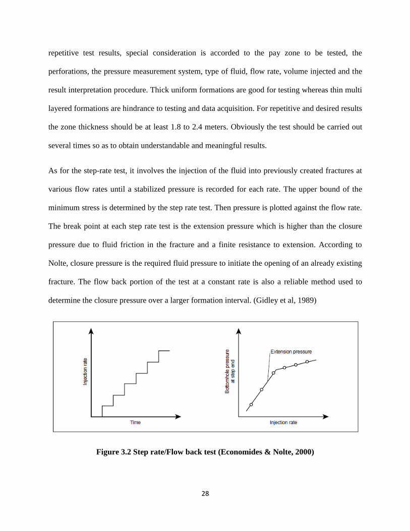
As for the step-rate test, it involves the injection of the fluid into previously created fractures at

various flow rates until a stabilized pressure is recorded for each rate. The upper bound of the

minimum stress is determined by the step rate test. Then pressure is plotted against the flow rate.

The break point at each step rate test is the extension pressure which is higher than the closure

pressure due to fluid friction in the fracture and a finite resistance to extension. According to

Nolte, closure pressure is the required fluid pressure to initiate the opening of an already existing

fracture. The flow back portion of the test at a constant rate is also a reliable method used to

determine the closure pressure over a larger formation interval. (Gidley et al, 1989)

Figure 3.2 Step rate/Flow back test (Economides & Nolte, 2000)

29

Reservoir pressure changes affect the in-situ stresses most especially during reservoir drawdown

and fracturing fluid leak off during hydraulic fracturing. During reservoir draw down, pore

pressure decreases leading to the volume shrinkage of the pore drained portion. The surrounding

impermeable layers laterally constrain the pores hence the attempted decrease in strain is

converted into decrease in stress. Meanwhile leak off of the fracturing fluid will lead to increase

in the in-situ stress and a consequent increase in the pore pressure.

3.2 ROCK PROPERTIES

There are various rock properties that are put into consideration prior to hydraulic fracturing

treatment. Some of the properties are; elasticity, Young‘s modulus, Poisson‘s ratio, shear

modulus, bulk modulus, and poroelasticity among others.

The general assumption that the rock is an elastic linear material simplifies the analysis of the

hydraulic fracturing problems. The principle of the rock acting as a linearly elastic material is

also applied during hydraulic fracturing modeling and development. Caution should be taken in

some instances whereby the rocks exhibit instances of nonlinearity.

Young‘s modulus is defined as the ratio of stress to strain as regards to the formation rock.

Young‘s modulus is applied in the computation of reservoir pressure and the fracture width

profile. The difference between the Young‘s modulus of the pay zone and the barrier rock affects

the fracture height growth.

Poisson‘s ratio is defined as the ratio of lateral expansion to longitudinal contraction of a rock

subjected to uniaxial stress. Poisson‘s ratio is essential in the determination of the fracture width

distribution and the in-situ stresses within the reservoir.

30

Poroelasticity relates to the effect of the formation pore pressure to the elastic deformation of the

reservoir rock. Increase in the pore pressure causes a respective volumetric expansion due to the

reduction of the effective stress caused by increased pressure. Formation fluids within the pore

support part of the applied stress to the formation. Hence when the reservoir rock undergoes

compression pore pressure increases as a result of the confinement within the pores. Change in

the pore pressure leads to change in the pore volume affecting the mechanical behavior of the

rock. The poroelastic material behaves in the similar way as an elastic solid under stress.

(Economides & Nolte, 2000)

The sonic log and density log are used to determine most of the rock mechanical and elastic

constants.

In-situ stresses and rock properties greatly influence the fracture azimuth and fracture geometry.

Fracture azimuth is defined as the direction of the fracture measured clockwise around the

observer‘s horizon from the north. Hubbert and Willis clearly state that the normal fracture

azimuth is the perpendicular to the minimum in-situ stress.

31

CHAPTER 4

HYDRAULIC FRACTURE MODELING

4.0 INTRODUCTION

Fracture modeling enables the understanding of some of the aspects that affect the fracture

geometry. Just like in all the other models applied in science, models are used to simulate real

life situations though on a small scale compared to the real scenario.

A model of a process can be described as a representation that captures the essential features of

the process so as to better understand the process (Starfield et al., 1990). There are three types of

models and they are; physical models, analytical models and empirical models. Physical models

are scale models of actual process. Empirical models are developed by observation using data

collected from laboratory or field work. Then, analytical models apply mathematical expressions

of the physical reality in which the governing mechanics are stated in the form of equations.

Analytical models are applied during hydraulic fracture modeling. Models are greatly applied

during hydraulic fracturing so as to quantify the volume of fluid and proppant required for a

specific formation treatment so as to justify the economics of the project and enabling the

prediction before the treatment or compare the after treatment fracture geometry. (Economides &

Nolte, 2000)

4.1 TWO DIMENSIONAL FRACTURE PROPAGATION MODEL

In the two dimensional models, one of the dimensions is fixed. Usually the fracture height is

fixed and the fracture width and length are calculated. Two dimensional models are usually used

when the fracture treatments required are small and the pump durations are relatively short.

32

(Holditch et al, 1987) The basis of accuracy of such a model depends on the accurate estimation

of the fracture height. Models in hydraulic fracturing are used to relate the fluid injection rate,

time of treatment and fluid leak off with fracture dimensions. The commonly known two

dimensional models assume a rectangular propagation model though radial or circular

propagation models are also rarely used. The most common two dimensional models are the

PKN and KGD models. The PKN model is commonly used when the fracture length is far

greater than the fracture height whereas the KGD model is used when the fracture height is far

greater than the fracture length. Such models are usually used so as to make hydraulic fracturing

treatment decisions during the design stage.

The initial work on hydraulic fracturing was published by Khristianovich & Zheltov (1955)

focusing on fluid flow and fracture mechanics. Thereafter, Perkins & Kern (1961) developed

models mainly considering fluid flow rendering fracture mechanics unimportant. Both works by

the two sets of groups mainly considered fracture geometry but did little about the issue of the

volume balance. Then, Carter (1957) developed another model that put into consideration the

volume balance but assuming constant and uniform fracture width. There were modifications to

the Khristianovich & Zheltov and Perkins & Kern models by Geertsma and de Klerk (1969) and

Nordgren (1972) respectively. This gave birth to the two basic two dimensional fracture

propagation models of hydraulic fracturing referred to as KGD and PKN models which were

named after the respective developers. These models considered the short fall of the previous

models and included volume balance and solid mechanics. The PKN and KGD models are used

today in the industry to design various formation treatments and they also applied in various

fracture modeling simulation computer software programs. (Economides & Nolte, 2000)

33

In summary, the Perkins and Kern assume that the fracture has an elliptical cross section in the

vertical plane with an opening proportionate to the fracture height. This assumption implies that

the fractures have narrower widths and they are longer while the pressure increases with fracture

growth. As for Khristianovich and Zheltov, they assume a rectangular vertical cross section of

the fracture whose width is controlled by its length which implies shorter and wider fractures

with constant extension pressure. However, it is worth noting that most hydraulic fractures relate

to the Khristianovich and Zheltov model. (Daneshy, 2009)

According to Holditch et al, two dimensional models have general assumptions made up by the

various original authors of the models. Some of the assumptions are; the formation is

homogenous and isotropic; formation deformation is derived from linear elastic stress strain

theory; the fracturing fluid is considered as a purely viscous liquid; gel and sand distribution

within the fracture are ignored and many more.

Both the PKN and KGD models are two dimensional fracture propagation models and they have

common assumptions. Both assume that the fracture will propagate in the direction perpendicular

to the minimum stress (planar). Both assume one dimensional fluid flow along the fracture.

Newtonian fluids are considered in both models. The rock in which the fracture propagates is

assumed to be continuous, homogeneous and isotropic linear elastic solid. A fixed vertical

fracture height is also considered for both.

4.1.1 PKN FRACTURE MODEL

PKN model was formulated by Perkins and Kern (1961) and later modified by Nordgren (1972)

hence the name.

34

The figure below shows a sketch of the PKN model where w stands for the width of the fracture,

L stands for length of the fracture and hf stands for the fixed vertical fracture height. The width

and length of the fracture change with time t as the distance x from the wellbore outwards along

the fracture length changes.

Figure 4.1 PKN fracture model (Economides & Nolte, 2000)

It assumes that each vertical cross section of the fracture acts independently implying that the

pressure in any of the sections is due to the height of the section rather than length of the

fracture, that is if the length of the fracture is much greater than the height. The model also

assumes a fixed vertical height fracture in the pay zone implying that the stresses in the strata

above and below the pay zone are large enough so as to inhibit any form of fracture growth. In

35

addition, the model assumes that the fracture cross section is elliptical and the width is maximum

at the cross section proportional to the net pressure at that point and independent of the width at

any other point. The model also assumes the hydraulic fracturing fluid pressure is constant in the

vertical cross sections perpendicular to the direction of fracture propagation. The model goes

ahead to assume that the fluid pressure gradient in the propagating direction depends on the flow

resistance within the fracture. There is also a general assumption that fluid pressure falls towards

the tip. For the case of the PKN model emphasis is on the effect of the fluid flow within the

fracture and the respective pressure gradients. The PKN model neglects the fracture mechanics

and the effect at the tip is ignored. (Economides & Nolte, 2000)

Initially, Perkins and Kern developed the model for non-Newtonian fluids then Lamb (1932)

adjusted the model for Newtonian fluids, then basing on this the net pressure will be;

𝑝𝑛𝑒𝑡 = 16𝜇𝑞𝑖𝐸

′3

𝜋𝑕𝑓4 𝐿

1/4

Where;

Pnet; Net pressure = Pressure in crack – Stress against which it opens

qi = Injection rate

μ = viscosity

The width of the fracture at any position along the length of the fracture is given by;

𝑤 𝑥 = 3 𝜇𝑞𝑖(𝐿 − 𝑥)

𝐸′

1/4

36

E’ stands for the plane strain deformation which is where planes(strata) that were parallel before

deformation remain parallel afterward and it is given by;

𝐸′ =𝐸

1 − 𝜈2

Where;

v = Poisson‘s ratio

E = Young‘s modulus

Perkins and Kern (1961) noted with concern that the average net pressure in the fracture greatly

exceeded the minimum pressure for fracture propagation unless the fluid flow rate was extremely

small or the fluid viscosity was drastically low. It should be noted that in real life hydraulic

fracturing, pressure due to fluid flow is far greater than the minimum pressure required for

fracture propagation implying that fracture propagation would continue till the pumping stopped

or if the leak off limited further extension or if the minimum pressure of fracture propagation

was reached. This justified the neglect of the fracture mechanics effects in this model. Initially

this model assumed plane strain behavior in the vertical direction. It also assumed fixed fracture

height. Leakoff and storage or volume changes in the fracture were neglected. The fracture

toughness was also neglected in this case.

Carter (1957) included leak off to the Perkins and Kern original model and he expressed the

leakoff velocity on the fracture wall by;

𝑢𝐿 =𝐶𝐿

𝑡 − 𝑡𝑒𝑥𝑝

37

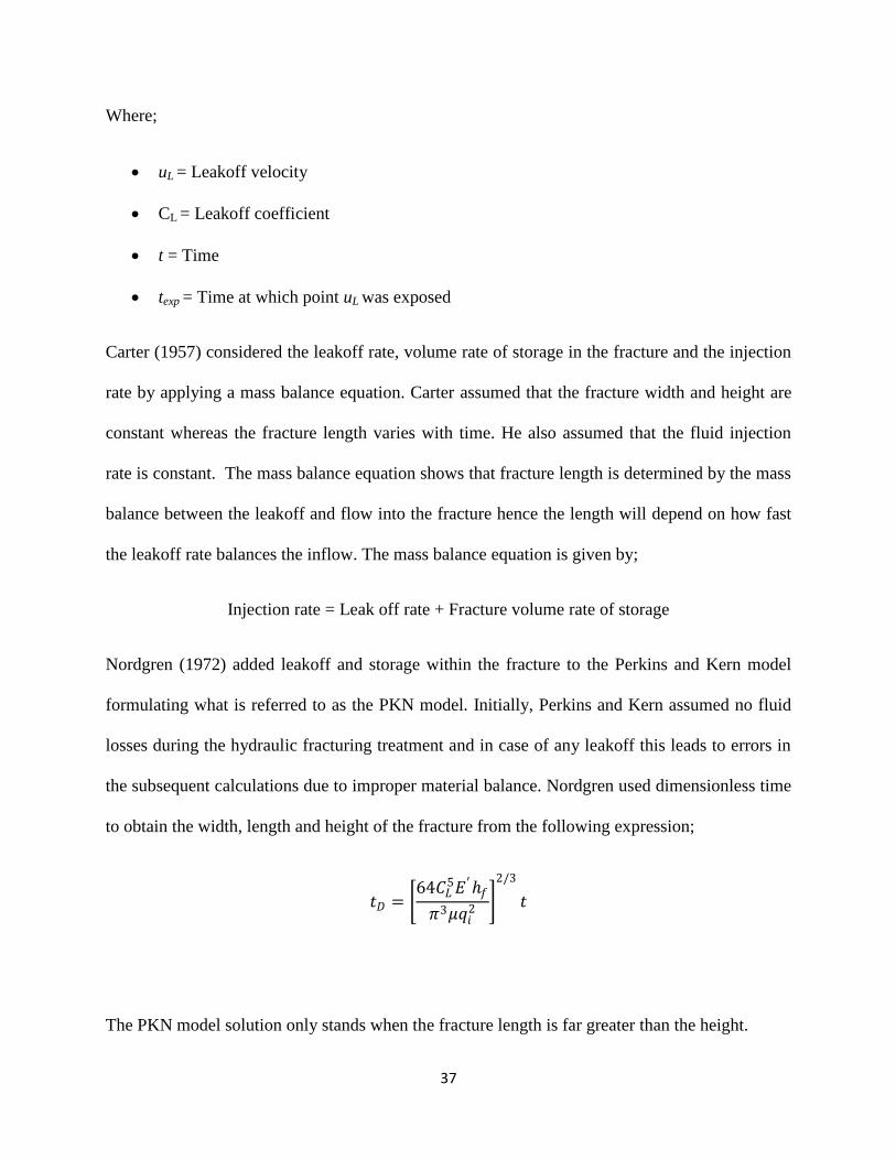
Where;

uL = Leakoff velocity

CL = Leakoff coefficient

t = Time

texp = Time at which point uL was exposed

Carter (1957) considered the leakoff rate, volume rate of storage in the fracture and the injection

rate by applying a mass balance equation. Carter assumed that the fracture width and height are

constant whereas the fracture length varies with time. He also assumed that the fluid injection

rate is constant. The mass balance equation shows that fracture length is determined by the mass

balance between the leakoff and flow into the fracture hence the length will depend on how fast

the leakoff rate balances the inflow. The mass balance equation is given by;

Injection rate = Leak off rate + Fracture volume rate of storage

Nordgren (1972) added leakoff and storage within the fracture to the Perkins and Kern model

formulating what is referred to as the PKN model. Initially, Perkins and Kern assumed no fluid

losses during the hydraulic fracturing treatment and in case of any leakoff this leads to errors in

the subsequent calculations due to improper material balance. Nordgren used dimensionless time

to obtain the width, length and height of the fracture from the following expression;

𝑡𝐷 = 64𝐶𝐿

5𝐸′𝑕𝑓

𝜋3𝜇𝑞𝑖2

2/3

𝑡

The PKN model solution only stands when the fracture length is far greater than the height.

38

4.1.2 KGD FRACTURE MODEL

Initially, Khristianovich & Zheltov (1955) assumed that the width of the crack at any distance

from the wellbore is independent of the vertical position. This model considered the fracture

mechanics that occur at the fracture tip.

Figure 4.2: KGD fracture model (Economides & Nolte, 2000)

This model assumes a constant flow rate within the fracture and a constant pressure within the

fracture apart from the fracture tip where there is no fluid penetration implying zero fluid

pressure. It also makes an assumption that the pressure in the main body of the fracture is almost

equal to the pressure at the well over most of the fracture length, with a sharp decrease near the

tip. The model also assumes fixed fracture height. Fluid pressure gradient in the propagating

direction depending on the flow resistance is also assumed.

39

Using Khristianovich & Zheltov assumption that the tip region is very small, Geertsma and de

Klerk simplified the model. The width of the fracture is given by;

𝑤𝑤 = 84𝜇𝑞𝑖𝐿

2

𝜋𝐸′𝑕𝑓

1/4

And the net pressure is also given by;

𝑝𝑛𝑒𝑡 ,𝑤 ≈ 21𝜇𝑞𝑖

64𝜋𝑕𝑓𝐿2𝐸′3

1/4

Ignoring the leakoff within the fracture;

𝐿 𝑡 = 0.38 𝐸′𝑞𝑡

3

𝜇𝑕𝑓3

1/6

𝑡2/3

𝑤𝑤 = 1.48 𝜇𝑞𝑖

3

𝐸′𝑕𝑓3

1/6

𝑡1/3

The volume of the two wing KGD fracture is given by;

𝑉𝑓 =𝜋

2𝑕𝑓𝐿𝑤𝑤

The various equations are quoted in this section are quoted from Economides & Nolte‘s book of

reservoir stimulation.

40

According to Holditch et al, there are several problems associated with the two dimensional

models. The commonest problem is the assumption of the fracture shape. It should be noted that

fractures do not take on simplistic shapes as assumed in most of the models because the low

permeability formation is multi layered with differing values of mechanical properties for the

respective layers. The other problem is the general assumption that fracture fluid leak off is

linear with respect to the square root of time which is not true for extended periods after fluid

leak off. Also the other problem is the assumption that the viscosity of the fracture fluids is

constant with time and space down the fracture which is not real in true life.

4.2 THREE DIMENSIONAL FRACTURE PROPAGATION MODEL

The two dimensional fracture propagation models of PKN and KGD assume a fixed fracture

height or assume that a radial fracture will develop after a fracturing treatment which is a

limitation to the application of the 2D models. In reality, the fracture height reduces towards the

fracture tip due to the waning effect of pump pressure towards the tip. 3D models represent the

formation elastic response when subjected to the hydraulic fluid pressure. Unlike in the 2D

models where fracture horizontal propagation is considered assuming that fracture height is

constant, 3D modeling considers all aspects of fracture geometry; that is the; height, length and

width with respect to hydraulic fluid pressure changing with time.

Application of 3D models accounts for the variation of fracture height with fluid injection which

is the reality. Usually 3D modeling is applied when the conventional 2D models cannot be

applied in hydraulic fracturing design. Three dimensional fracture propagation models involve

the division of a fracture into individual elements and solving the complex equations as

pertaining to the elements using digital computer software. The equations considered involve;

41

elasticity equations of the fracture opening in the rock, fluid flow equations and the consideration

of the stress ahead of the fracture to the tensile stress required for fracturing the rock.

In three dimensional fracture propagation modeling, the formation is considered to be a linear

elastic solid when subjected to the pressure due to the hydraulic fracturing fluid. Also, poro

elasticity effects of the formation are neglected. In 3D modeling, isotropic elasticity is assumed.

The formation is assumed to be infinite in extent because the pay zones are located at great

depths compared to fracture dimensions. The fracture is assumed to develop as a plane, vertical

fracture oriented perpendicular to the direction of the minimum in-situ compressive stress.

(Gidley et al, 1989)

Three dimensional fracture propagation modeling enables realistic prediction of the fracture

geometry, proppant distribution and treatment performance during hydraulic fracturing design.

According to Economides & Nolte, there are three types of three dimensional models; general

3D, planar 3D and pseudo-3D (P3D) models.

The general 3D models do not make any assumptions as regards to the fracture orientation and

they are commonly for research purposes. Planar 3D models assume that the fracture is planar

and oriented perpendicular to the minimum in-situ stress. Such models are used in treatments

where a considerable portion of fracture volume is outside the zone where the fracture initiates or

where there is more vertical than horizontal fluid flow. This evident when the in-situ stresses of

the top or bottom layers are equal or below stresses of the pay zone.

Pseudo-3D models are classified into lumped (elliptical) and cell based. Lumped models assume

that the vertical fracture profile consist of two half ellipses joined at the center. Such models

assume a stream line fluid flow of a particular shape. Cell based models assume that fractures are

42

like a series of connected cells and also plane strain is assumed. The planar and pseudo-3D

models rely on the data of the layers around the pay zone to predict fracture growth in these

layers. Three dimensional fracture propagation models are mainly used by the simulators during

computational applications to obtain the required parameters during the formation treatment

process. (Economides & Nolte, 2000)

4.2.1 PLANAR THREE DIMENSIONAL MODELS

A planar fracture can be described as a narrow channel whose width varies with fluid flow. The

fracture width varies with time depending on the pressure variation due to fluid flow within the

fracture hence fracture geometry is greatly influenced by fluid flow.

The fracture shape changes with time depending on the applied fluid pressure to fracture the rock

at the boundary and this is best described by linear elastic fracture mechanics (LEFM). If the

LEFM of the rock is exceeded at the tip, the fracture will extend until the criterion is met again.

Complex equations derived from the planar 3D models require a computerized numerical

simulation so that they can be solved. Most of the equations are basically conceptual due to the

complex modeling process arising from the non linear relationship between the width and

pressure and the overall complexity of the moving fracture boundary problem.

Clifton and Abou Sayed (1979) computed the first numerical implementation of the planar 3D

model by dividing the fracture into equal elements, 16 squares to be specific and then applying a

solution of equations. They considered that as the boundary of the fracture extends, the elements

also adjust to accommodate the new fracture shape. The limitation of this method was that

elements develop large aspect ratios and very small angles.

43

Figure 4.3; Clifton & Abou Sayed (1979) planar 3D representation in the form of squares

(Economides & Nolte, 2000)

Then, Barree (1983) divided the layered reservoir into equal sized rectangular elements over the

entire area that the fracture might cover. For his case, he considers that the grid of elements does

not move when the criterion is exceeded but the elements ahead of the failed tip just open to the

flow becoming part of the fracture. The limitations of this formulation are; the number of

elements in the simulation increases as the simulation proceeds therefore if the initial number of

elements is small this leads to inaccuracies; also this formulation requires that the general size of

the fracture must be estimated in advance of the of the simulation to ensure that a reasonable

number of elements are used.

44

Figure 4.4; Barree (1983) fixed grid solution (Economides & Nolte, 2000)

4.2.2 PSEUDO THREE DIMENSIONAL MODELS

4.2.2.1 CELL BASED PSEUDO THREE DIMENSIONAL MODELS

Cell based pseudo three dimensional models consider the fracture length to be divided into

various cells. The model assumes horizontal fluid flow along the length of the fracture and plane

strain at any cross section for solid mechanics.

One dimensional fluid flow implies pressure in the cross section is given by;

𝑝 = 𝑝𝑐𝑝 + 𝜌𝑔𝑦

Whereby 𝑝𝑐𝑝 is the pressure along the horizontal line through the center of the perforations and

y is the distance from the center of the perforations. The above equation assumes that the vertical

tips of the fracture are almost stationary at all times and this is referred to as the equilibrium

height assumptions. 1

45

Basing on the equilibrium height assumption, solid mechanics solution is used to determine the

cross sectional fracture shape as a function of net pressure. This solution was derived by

Simonson et al. (1978) for a symmetrical three layer formation and later a general solution for

non symmetrical layers was developed by Fung et al. (1987). The stress intensity factors of both

bottom and top fracture tips are used to determine the fracture geometry.

In the case of the fluid mechanics solution, both vertical fluid flow and variation of horizontal

velocity as a function of vertical position are neglected leading to failure of the model to

represent various issues like; effect of variation of vertical width on fluid velocity, local

dehydration, fluid loss after tip screen outs when fluid flows through the proppant pack is

ignored and proppant settling due to convection or gravity currents. (Economides & Nolte 2000)

4.2.2.2 LUMPED PSEUDO THREE DIMENSIONAL MODELS

This form of three dimensional modeling was first introduced by Cleary (1980). The model is

used in the development of computer software used in hydraulic fracturing treatment to

determine the various parameters. Some of the characteristics of the software are; realistic and

general physics is upheld, execution time is much faster than the treatment time and software can

use real time improved estimates of parameters obtained in real time. With the advancement

technology by the day now days, this software application is bound to be improved with time.

However, the accuracy of this model largely depends on the appropriate selection of coefficients

used for the problem analysis.

During the lumped pseudo three dimensional modeling the following equations are applied; mass

conservation, relation between the distribution of fracture opening over the length of the fracture

and the net pressure distribution equation. For the simplicity of the equations, the fracture shape

46

consisting of two half ellipses of equal lateral extent but different vertical extent is assumed and

also a spatial averaging is utilized.

However, 3D modeling comes with increased cost of obtaining the additional information on the

formation properties and less computing time. Vital additional information includes variation of

the minimum in situ stress with depth and changes in elastic moduli from layer to layer.

In the near future, 3D modeling is expected to be the benchmark for any hydraulic fracturing

simulation in this technologically evolving world of today. To date the world‘s main oil and gas

production plus service companies use 3D modeling to make crucial decisions as regards to

hydraulic fracturing where 2D modeling has been found wanting due to inadequate information.

Most oil and gas companies are developing in house 3D modeling software so as to make work

easy for the fracture designers. Some of the hydraulic fracturing software on the market includes;

StimPlan by NSI Technologies, MFrac by Baker Hughes, Mangrove Reservoir stimulation

Design Software by Schlumberger.

Some of the examples of planar 3D models are TerraFrac and HYFRAC3D. Common examples

of pseudo-3D models are StimPlan, ENERFRAC, TRIFAC, FRACPRO and MFRAC-II. The

examples of classic PKN and KGD models are PROP, the chevron 2D model, the Conoco 2D

model and the shell 2D model. (Warpinski et al, 1994)

47

CHAPTER 5

FRACTURE HEIGHT CONTROL

5.0 INTRODUCTION

Fracture height growth is mainly governed by the in-situ stress differences existing between

formation layers. In case the in-situ stress differences between the formation layers are negligible

then the slip on bedding planes or fracture toughness contrast between the layers is considered.

Fracture toughness is the measure of resistance of the rock to the generated fracture propagation.

However, the direction of fracture propagation is usually perpendicular to the axis of the

minimum stress in the formation.

During two dimensional fracture modeling the fracture height is assumed to be constant while

the complex pseudo three dimensional models are used to calculate fracture height by

undertaking some assumptions. Fracture height containment greatly depends on in-situ stress

differences, young‘s modulus, fracture toughness, interface slippage among others.

In-situ stress differences between the pay zone and the upper and a lower bounding formation

layer is the main factor that influences fracture height growth. Usually the fractures propagate to

a greater extent into the upper layer of less stress compared to the lower layer which is normally

of a higher stress. This section of the report is interested in the determination of the fracture

height and the factors that influence fracture height containment.

5.1 DETERMINING FRACTURE HEIGHT

Post fracture temperature logs are used in the measuring of fracture height after hydraulic

fracturing. It involves determination of the prefracture temperature profile by logging followed

48

by at the least two postfracture temperature logs. The process entails running a pre fracture

temperature log so as to determine the temperature gradient in the reservoir formation and

thereafter temperature logs are run after the hydraulic fracturing stimulation process. Heat

transfer in the surrounding layers is by conduction whereas in the fractured payzone it is by

convection. On interpreting the temperature logs, a temperature anomaly is noticed due to the

different temperature recover rates after pumping hence identifying the fractured zone.

Just like any other logs, sometimes errors occur as a result of information misinterpretation and

this may be due to fracture deviation from the well bore. 2 The other limitation of temperature

logs is that they only detect fractures very near to the wellbore. Postfracture temperature log

analysis is greatly affected by the fracture width and fracture height whereby formations of low

stress and low modulus tend to have wider fracture width hence taking in more fracturing fluid

leading to more cooling in the zone coupled with the largest temperature anomaly adjacent to the

fracture. On the positive side, this clearly indicates the payzone of interest where the fluid is

going and on the negative side the large anomaly can mask height growth leading to false

misinterpretation regarding fracture geometry. The wellbore condition also affects the analysis of

the temperature logs because of the temperature anomaly below the tubing due to difference in

radial heat flow rates for the tubing compared to the fluid flow inside the casing. (Gidley et al,

1989)

These limitations can be overcome by executing more than one postfracture temperature log so

as to minimize errors in analysis. Dobkins (1981) also suggested the use of a cold water

circulating test so as to improve the temperature log analysis. Water is circulated down the

tubing and up through the annulus cooling the well bore. Then logs are run indicating changes in

the thermal conductivity and thereafter postfracture temperature logs are run and any deviation

49

from the initial response points to fluid movement outside the pipe showing fracture height

growth.

Also, radioactivity logs and noise logs are used during fracture height measurement. The noise

logs use the hydrophone to detect fluid movement outside the casing. Noise logs are usually used

in conjunction with other methods so as to determine the fracture height. The radioactivity logs

involve inducing radioactivity by the inclusion of tagged sand material in the proppant then

followed by the gamma ray log. The advantage of using the radioactivity log is they do not need

to be run immediately after the stimulation enabling the removal of the wellbore fill below the

perforations before logging. Just like in the temperature logs the limitation of radioactivity log is

that it is only applicable near the wellbore. 1 Also the radioactivity logs are unable to

differentiate between a fracture and a small channel behind the casing. (Economides & Nolte

2000)

Fracture height is also measured by direct measurement and such methods yield more data as

compared to other methods. Impression packers, sonic borehole televiewers (BHTV‘s) and

downhole television cameras are applied during the direct measurement of fracture geometry.

Impression packers are used in the determination of the fracture azimuth although they are not

reliable when it comes to fracture height determination.

50

Figure 5.1; Impression packer application schematic (courtesy of

http://www.hydrofrac.com/hfc_setup.html)

The BHTV contains a crystal inside the tool that emits a pulse then records its reflection from the

borehole wall. Lack of reflection implies that the fracture width is larger than the wave length of

the sonic signal. Downhole television cameras involve the injecting of fluid into the formation

and the resulting fracture geometry recorded on a videotape.

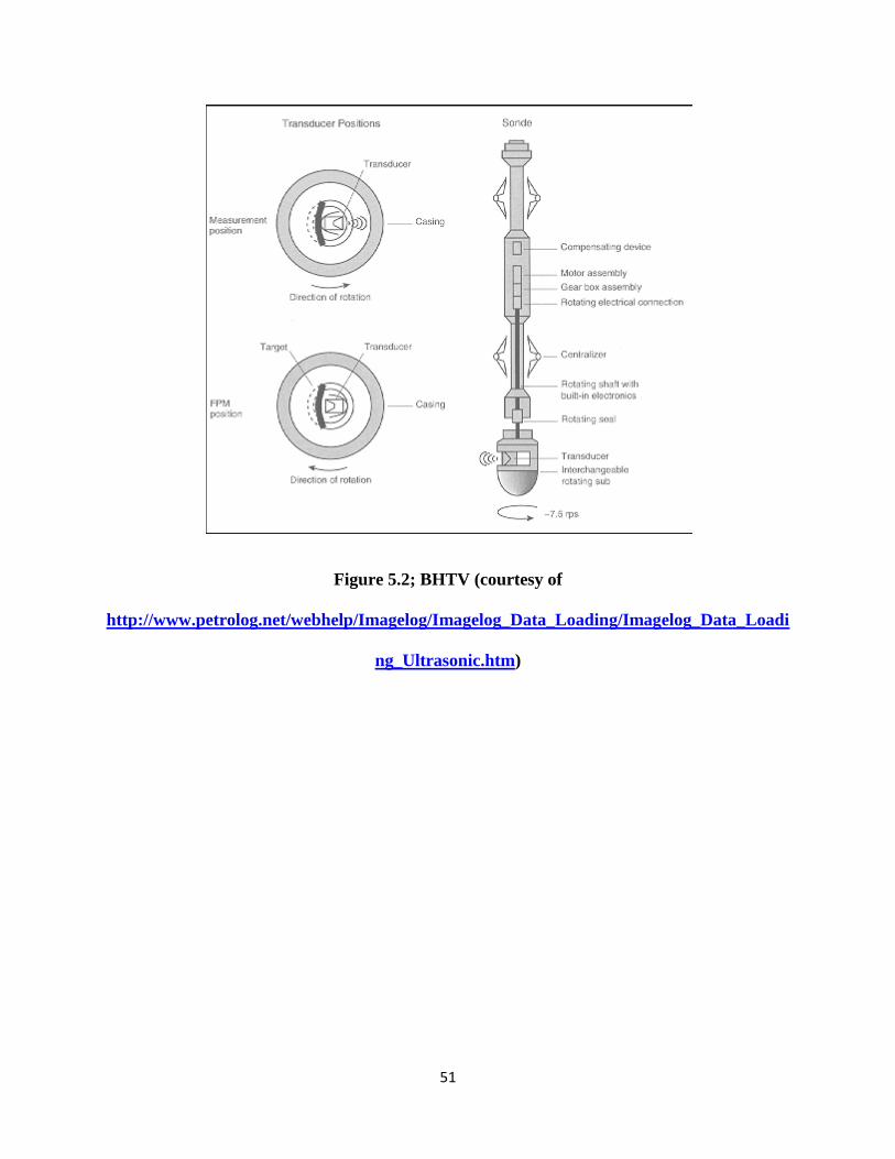
51

Figure 5.2; BHTV (courtesy of

http://www.petrolog.net/webhelp/Imagelog/Imagelog_Data_Loading/Imagelog_Data_Loadi

ng_Ultrasonic.htm)

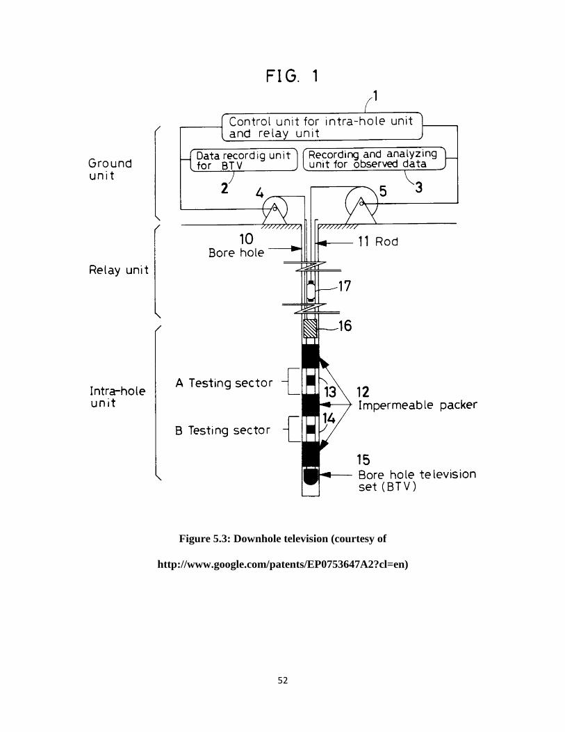
52

Figure 5.3: Downhole television (courtesy of

http://www.google.com/patents/EP0753647A2?cl=en)

53

Also, fracture mapping technologies like microseismic and microdeformation are readily applied

to determine the fracture height of the industrial hydraulic fractures. These technologies are

usually for confirmation for the measured fracture height. Microseismic fracture monitoring

determines fracture height by detecting and locating the minor reservoir movements

(microseism) caused by the hydraulic fracturing process as a result of variation in the formation

stresses during fracture opening. The process involves the positioning long arrays of sensitive

receivers in offset wells that are close to the payzone. Receivers detect the small formation

movements in the form of compressional and shear waves depending on the wave arrival times

and polarizations. The larger the microseism and the corresponding noise generated during

fracturing the easier it is for the receivers to detect the movements hence the easier it is to

determine the resulting fracture height.

Microdeformation fracture monitoring involves the determination of fracture height by

measurement of the small reservoir movements on the earth‘s surface or sub-surface (observation

well) using tiltmeters. Apart from determining the fracture height, tiltmeters are also used to

determine; the reservoir deformation pattern, fracture orientation, fracture azimuth and fracture

dip. (Fisher & Warpinski 2011)

5.2 FRACTURE HEIGHT CONTROL

Control of fracture height growth or say fracture containment is achieved by stress contrast,

modulus contrast, fracture slippage and fracture re-orientation near an interface. The latter is

common in coal mines. Fracture height control is aimed at containment of reservoir fluid,

production of unwanted water or gas, optimizing reservoir production and protection of

underground water aquifers among others.

54

Fracture height growth occurs when the existing local stresses exceed the resistance of the

formation to fracturing. Fracture growth in all directions will always take the direction of least

resistance say of the least pressure. Once a fracture growth encounters a region of requires a

higher pressure so as fracture growth can be achieved, it stagnates at that point till the required

pressure is achieved for extension.

Simonson et al stated that the formation layer with a higher Young‘s modulus acts as a barrier of

fracture height growth from a lower modulus formation layer. In contrast, Daneshy and field

experiments carried out by Sandia National Laboratory at Nevada Test Site proved that the

elastic moduli contrast is not enough to curb fracture growth across the formation interface.

Daneshy further showed that shear sliding of the fracture at interfaces blunts the fracture tip

hence proving fracture containment and this was later confirmed by the experimental work of

Anderson. (Daneshy, 2009)

Literally, higher stresses in the bounding adjacent layers are responsible for fracture height

containment. Basing on Teufel‘s experiments and numeric investigations, fracture containment is

achieved by the increasing the minimum horizontal stress in bounding adjacent layers and low

shear strength along the interface. According to experiments and observations by Warpinski et

al, stress contrast or fracture toughness variations are not only the factors behind fracture

containment but also slippage at the interfaces.

Barree et al fronts shear plane slippage as the primary reason for fracture height containment.

They observed that discontinuous fracture surfaces separated by shear fractures and planes

reduce the stress at the fracture tips. They also argue that the flow of the fracturing fluid in the

existing or induced fractures reduces friction resistance of these surfaces to sliding leading to the

55

blunting of the fracture tip hence height containment. They also showed that the created fractures

have narrower widths which reduce the pressure for the fracture to cross an adjoining boundary.

Shear fracturing within the formation also affects the fracture growth in terms of the length and

height. During fracturing the forces in the fracture plane as a result of the fluid injection create a

substantial leverage and tensile stresses at the fracture tips way higher than the formation

strength leading to fracture growth. The generated stresses are greatly influenced by the available

surface area of the fracture. Presence of shear fractures along the fracture surface area fragments

the available fracture surface area causing discontinuity in the fracture area reducing its leverage.

This leads to the dissipation of most of the force on shear fracture growth instead of being

exerted on fracture tips. Hence the discontinuity in fracture growth due to the shear fractures

reduces the rate of fracture growth.

The reason for fracture height control is to curb fracture penetration into undesirable zones like

the gas cap, water bearing zones or unproductive zones while maximizing lateral fracture

extension within the payzone hence increasing productivity. Hence uncontrolled fracture height

growth can lead to unwanted gas or water production. (Vatsa & Wang, 2011) Also uncontrolled

fracture height growth leads to loss of production into the upper or lower barrier layers lowering

production estimates. Fracture height growth beyond the pay zone leads to failure of the

achievement of the optimum lateral extension fracture due to wastage of the proppant and

pumping energy in propagating the fracture out of zone. Fracture height growths beyond the pay

zone may lead to the penetration into a high permeability formation layer leading to excessive

leakoff or ineffective fractures and if it is not controlled this can end up in the shallow water

zone. Control of fracture height growth also avoids wastage of fluid, pump horse power,

56

chemicals, time and labor out of the payzone which improves the economic viability of the

project. (Larson & Nguyen, 1984)

5.3.1 FRACTURE HEIGHT CONTAINMENT

Fracture height containment mechanisms are divided into three categories, namely; natural

factors, artificial factors and formation response to fluid invasion. The natural factors deal with

the formation in-situ conditions that influence fracture height propagation like stress contrasts,

in-situ stress gradients, elastic or plastic behavior, toughness, discontinuities and natural

fractures, fracturing fluid leakoff and heat transfer properties. The artificial factors relate to

injection characteristics like flow rate and rheology, proppant placement and temperature

profiles. Then finally the formation response to fluid invasion may induce back stresses, poro-

elastic and thermoelastic effects in the formation. (Naceur & Touboul 1990)

Naturally, according to Warpinski et al and other authors, the predominant factor for fracture

height containment is the barrier in-situ stresses contrast between the payzone and the formation

layers surrounding the payzone. Fracture height growth is contained when the in-situ stresses of

the upper and lower boundary formation layers are higher than the stresses initiated in the

payzone during hydraulic fracturing. Simonson et al states that for in-situ stress gradients larger

than the hydraulic fluid gravity, the fracture has a tendency to vertically migrate reducing the

fracture coverage of the pay zone. Depending on the formation stresses fracture height growth is

controlled by regulating the pump injection rates or using fluid with low viscosities to avoid

exceeding a critical pressure that might lead to excessive unwanted fracture height propagation

out of the payzone.

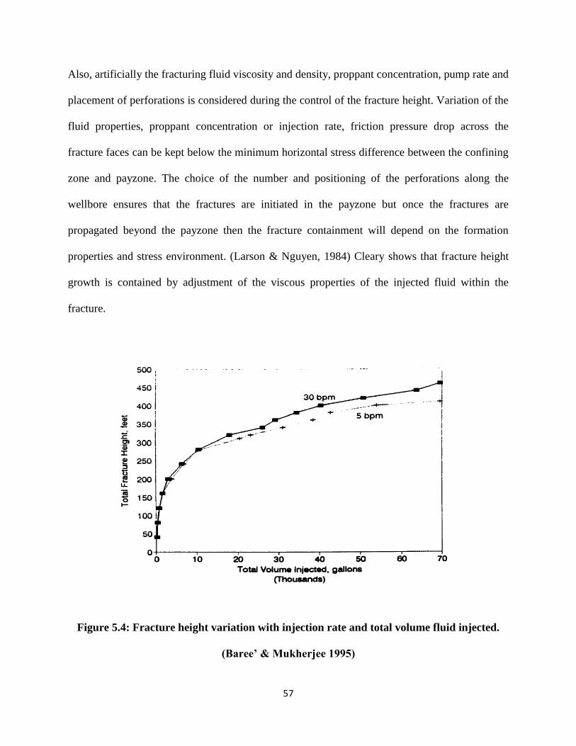
57

Also, artificially the fracturing fluid viscosity and density, proppant concentration, pump rate and

placement of perforations is considered during the control of the fracture height. Variation of the

fluid properties, proppant concentration or injection rate, friction pressure drop across the

fracture faces can be kept below the minimum horizontal stress difference between the confining

zone and payzone. The choice of the number and positioning of the perforations along the

wellbore ensures that the fractures are initiated in the payzone but once the fractures are

propagated beyond the payzone then the fracture containment will depend on the formation

properties and stress environment. (Larson & Nguyen, 1984) Cleary shows that fracture height

growth is contained by adjustment of the viscous properties of the injected fluid within the

fracture.

Figure 5.4: Fracture height variation with injection rate and total volume fluid injected.

(Baree’ & Mukherjee 1995)

58

According to experiments by Tushar & Wang (2011), the choice of the injection rate for the

fracturing fluid used during fracture treatment affects the fracture height growth within or

beyond the payzone. The injection rate coupled with the fracture conductivity of the fracturing

fluid used is optimized so as to contain the fracture within the payzone. If the injection rate is too

high then the fracture will propagate beyond the payzone which is undesirable whereas if the

injection rate is too low this leads to under productivity since the payzone is not fully covered by

the resulting fracture geometry. The injection rate or pump rate affects the fracture height growth

especially when the minimum in-situ stress contrast between the payzone and the bounding

layers is small. (Liu et al, 1998) The choice of the fracturing fluid affects the fracture

conductivity which influences the fracture height growth. Properties of the chosen fracturing

fluid like the fluid viscosity greatly determine the fracture propagation.

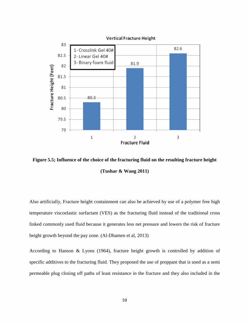
59

Figure 5.5; Influence of the choice of the fracturing fluid on the resulting fracture height

(Tushar & Wang 2011)

Also artificially, Fracture height containment can also be achieved by use of a polymer free high

temperature viscoelastic surfactant (VES) as the fracturing fluid instead of the traditional cross

linked commonly used fluid because it generates less net pressure and lowers the risk of fracture

height growth beyond the pay zone. (Al-Dhamen et al, 2013)

According to Hanson & Lyons (1964), fracture height growth is controlled by addition of

specific additives to the fracturing fluid. They proposed the use of proppant that is used as a semi

permeable plug closing off paths of least resistance in the fracture and they also included in the

60

fluid plastically deformable solids having densities equal to or different from the fluid. (Hanson,

1964)

Artificially, Fracture height growth is also controlled by the selective placement of artificial

barriers above and below the pay zone ensuring that the front tip of the fracture is open to lateral

extension. Artificial barrier placement requires the understanding of the proppant movement

which involves the floatation and settling of the proppant which depends on the proppant density

and the convective movement of the particle slurry. The use of artificial barriers is considered

when the stress barriers of the upper and lower formations fail to contain fracture height growth.

Initially the pay zone is fractured creating a fracture channel. This is then followed by the

injection of different sized and density proppants carried by a low viscosity fluid allowing

floatation or settling of the proppants at the top or bottom of the fracture channel respectively.

Usually the heavier proppant settles at the bottom and the light proppant floats at the top of the

fracture channel inhibiting any growth at the fracture tips. Upon successful barrier placement, the

hydraulic fractures are confined within the proximities of the barriers curbing fracture height

growth though leading to the horizontal extension of the fracture in the pay zone. Beyond these

barriers the fracture loses any form of artificial fracture height containment and propagates

according to the formation stress profile. (Baree‘ & Mukherjee, 1995) The lateral fracture

extension leads to post fracture production increase plus enhancing load fluid recovery. 7

According to Mukherjee et al (1995), the techniques for barrier placement are Invertafrac –

barrier above the pay zone, Divertafrac – barrier below the payzone and Bracketfrac – barriers

above and below the pay zone.

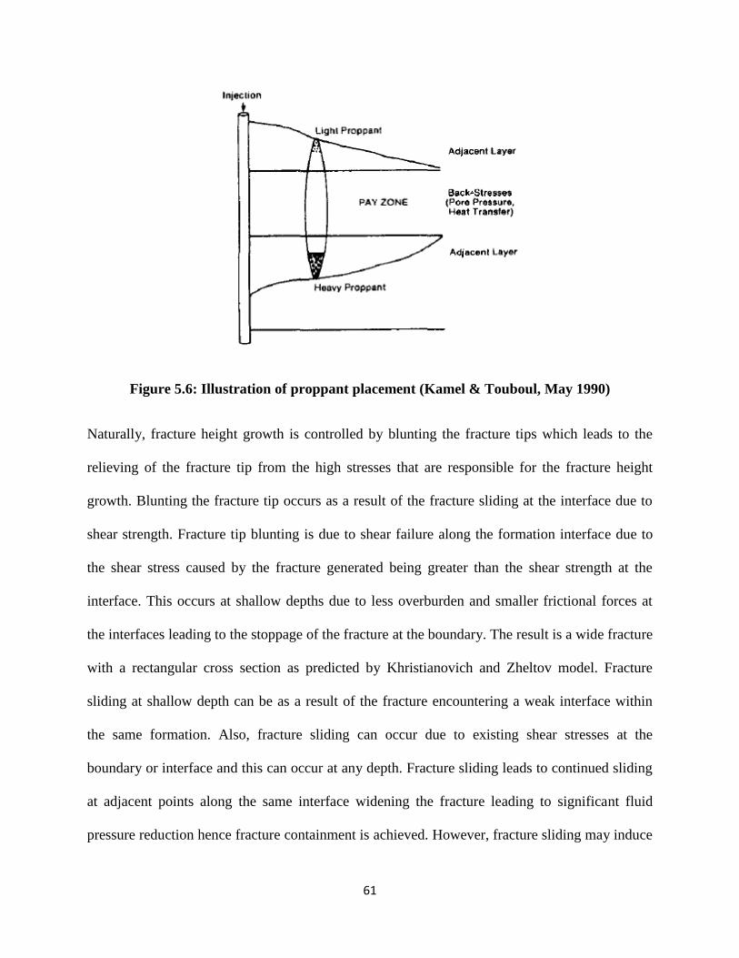
61

Figure 5.6: Illustration of proppant placement (Kamel & Touboul, May 1990)

Naturally, fracture height growth is controlled by blunting the fracture tips which leads to the

relieving of the fracture tip from the high stresses that are responsible for the fracture height

growth. Blunting the fracture tip occurs as a result of the fracture sliding at the interface due to

shear strength. Fracture tip blunting is due to shear failure along the formation interface due to

the shear stress caused by the fracture generated being greater than the shear strength at the

interface. This occurs at shallow depths due to less overburden and smaller frictional forces at

the interfaces leading to the stoppage of the fracture at the boundary. The result is a wide fracture

with a rectangular cross section as predicted by Khristianovich and Zheltov model. Fracture

sliding at shallow depth can be as a result of the fracture encountering a weak interface within

the same formation. Also, fracture sliding can occur due to existing shear stresses at the

boundary or interface and this can occur at any depth. Fracture sliding leads to continued sliding

at adjacent points along the same interface widening the fracture leading to significant fluid

pressure reduction hence fracture containment is achieved. However, fracture sliding may induce

62

high tensile stresses at the interfaces leading to initiation of new fractures in the adjacent

formation. Fracture growth or slippage is evident in lower pressure areas. However, Daneshy

basing on field evidence states that fracture blunting may not guarantee total fracture

containment because the fracture has a very long fracture tip and it can grow at other points or

even grow backwards towards the blunted tip.

Naturally, fracture height growth is also controlled by the fracture re-orienting near the interface.

This has been observed using micro-seismic and tiltmeter surveys leading to what are referred to

as ―T shaped‖ fractures. T-shaped fractures consist of a horizontal and vertical fracture joined

together hence the name. In this case, the horizontal fracture extension pressures are below the

overburden stress. Hence the vertical principal stress in the fractured formation is less than the

overburden leading to the horizontal fracture growth at lower pressures. (Daneshy 2009)

Naturally, fracture height containment is achieved as a result of geologic discontinuities like

joints, faults, and bedding planes. This leads to the formation layer stress contrasts, cohesionless

interfaces and so on which lead to fracture containment. Faults lead to termination of fracture

height growth or in case they propagate there is change in the orientation of the fracture and this

is caused by the change in stress across the fault. Joints within the formation also lead to

offsetting the hydraulic fracture leading to some of the fractures dying out or even persisting for

long distances. In some rare instances the fractures may be initiated from such joints within the

formation during hydraulic fracturing treatment. According to Teufel and Clark (1984) and

Anderson (1981) laboratory experiments, fractures appear to terminate at the bedding planes

(parting plane or zero bonding plane) or propagate a short distance across the plane before dying

out due to the presence of sufficient friction. Hence bedding planes and stress contrasts are vital

for fracture containment and in situations where friction is less; the bedding plane can be an

63

efficient fracture height growth barrier. The effect of the geologic discontinuities on fracture

height containment depends on the permeability of the joints, frictional properties, in-situ

stresses, joint spacing and orientation, treatment pressure and fracture fluid leakoff

viscosity.(Warpinski & Teufel, 1987)

Figure 5.7 Mineback experiment showing the termination of the fracture near the fault

(Warpinski & Teufel, Feb 1987)

64

Figure 5.8; A mineback fracture near borehole (white) offset at the natural fracture

creating two fractures on intersecting the natural fracture (Fisher & Warpinski 2011)

Figure 5.9; Mineback photograph (and line drawing) of fracture kinking, offsetting and

turning as bedding planes (interfaces) are crossed (Fisher & Warpinski 2011)

65

Figure 6.0: Visualization of fracture treatment in a jointed formation (Warpinski & Teufel,

Feb 1987)

66

CHAPTER 6

CASE STUDY; INVESTIGATION OF RELATIONSHIP BETWEEN UNDERGROUND

WATER AQUIFER CONTAMINATION AND FRACTURE HEIGHT GROWTH

6.0 INTRODUCTION

In this section, I review one of the most controversial issues as regards to the application of the

hydraulic fracturing technology which is; hydraulic fracturing leads to underground water

aquifer contamination. Most environmentalists or green peace activists are using this issue to

discredit the application of the process in the production of hydro carbons from tight reservoirs.

They argue that the process leads to fracturing into water aquifers leading to contamination of

water with hydrocarbons, fracturing fluids and so on. There is an argument that methane gas sips

through the generated fractures to the aquifers leading to contamination. I am going to critically

analyze both scientists that argue for and against and at the end of it all I will give my stand.

Most of the field data and references in this section are taken from field development data from

North America and USA to be specific since hydraulic fracturing use is prevalent and well

documented in this part of the world.

For this case study, emphasis is put on aquifer contamination through the upward migration of

the hydrocarbons (methane) through the generated hydraulic fractures. According to various

literature sources, hydraulic fracturing mainly leads to water contamination through, poor

handling and disposal of; chemicals used in the process, produced and flow back waters; gas

leaks through casing and generated hydraulic fracture and natural fractures connectivity with the

water aquifers. (Vengosh et al) For this section emphasis is aimed at the latter cause and

investigating its cause in relation to the water contamination.

67

6.1 ARGUMENT FOR

Other than aquifer contamination through leakage of fracturing fluid or hydrocarbons,

contamination is probable through the leakage of biogenic or thermogenic gas from the

formation behind the well casing (casing leaks), or even the upward natural migration of the gas

over a long period of time. (Davies et al, 2012) But the chances if the gradual natural upward

migration of the hydrocarbon into the aquifers is slim due to the presence of the cap rock which

ensures that the hydrocarbon is contained hence enabling its accumulation that leads to

economically viable reservoir production. This happens due to human error leading to poor

cement jobs attributing to casing leaks which with upward migration ends ups into water

aquifers. Also with age the casing rusts leading to gas leakage into the aquifers. (James, 2011)

Figure 6.1: Illustration of the possible forms of casing leaks (Alberta Energy Utilities

Board)

68

Osborn et al (2011) demonstrated methane water aquifer contamination in the Marcellus and

Utica shale plays located in the north east of Pennsylvania and upstate New York due to the

application of hydraulic fracturing in the shale gas extraction. The methane concentration in the

water increased more towards the gas producing well sites compared to non - producing sites of

the same geology and hydrogeologic regimes. The distinction between the methane sources is

based on the different isotopes (δ13

C-CH4; δ2H-CH4) and the geochemical compositions (ethane

/propane ratios).Water tested near the shale gas wells was detected to have excessive amounts of

C-CH4 than those located at about one kilometer away. As for the gas producing sites, the

average and maximum methane concentration in the water was found to be at 19.2 and 64

milligrams per liter respectively which is potentially an explosion hazard. When the methane

concentration in the water exceeds 10milligrams per liter then it‘s considered as a hazard. The

non producing sites were discovered to have an average concentration of 1.1 milligrams of

methane per liter of water. They attribute the lower methane concentration in water aquifers near

the non-productive sites to the natural biogenic sources. Thermogenic methane originates from

the shale formations deep underground whereas biogenic methane is synthesized by microbes

located nearer to the surface close to the aquifers. (Mooney, 2011)

However they further point out that following the laboratory tests, there was no form of water

aquifer contamination was found as a result of the fracturing fluids. The depth of the drinking

water wells in 60-90 meters and the vertical distance between the shale and the water zone is

900-1800 meters. Also worth noting is that the research area is characterized by faults,

earthquakes and so on. Osborn et al attribute the methane migration to; casing leaks of gas wells

leading to upward migration through the formation fracture systems, and generated hydraulic

fractures or enlargement of existing fractures above the payzone acting as conduits for the

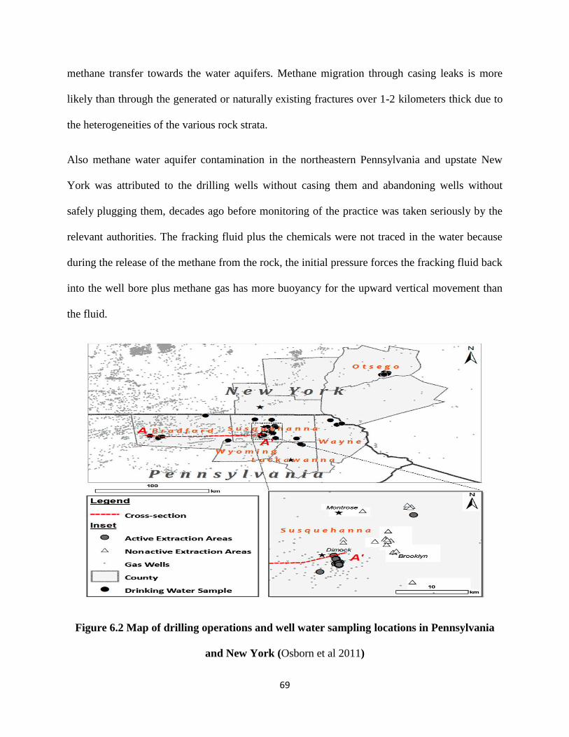
69

methane transfer towards the water aquifers. Methane migration through casing leaks is more

likely than through the generated or naturally existing fractures over 1-2 kilometers thick due to

the heterogeneities of the various rock strata.

Also methane water aquifer contamination in the northeastern Pennsylvania and upstate New

York was attributed to the drilling wells without casing them and abandoning wells without

safely plugging them, decades ago before monitoring of the practice was taken seriously by the

relevant authorities. The fracking fluid plus the chemicals were not traced in the water because

during the release of the methane from the rock, the initial pressure forces the fracking fluid back

into the well bore plus methane gas has more buoyancy for the upward vertical movement than

the fluid.

Figure 6.2 Map of drilling operations and well water sampling locations in Pennsylvania

and New York (Osborn et al 2011)

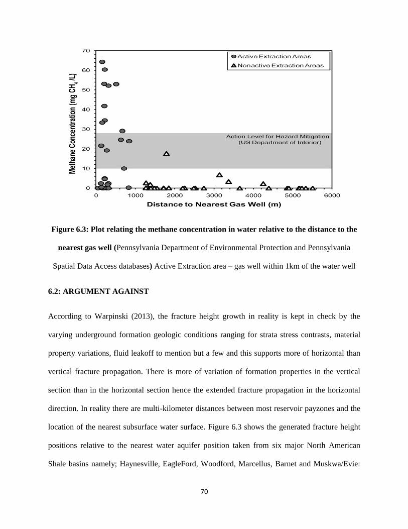
70

Figure 6.3: Plot relating the methane concentration in water relative to the distance to the

nearest gas well (Pennsylvania Department of Environmental Protection and Pennsylvania

Spatial Data Access databases) Active Extraction area – gas well within 1km of the water well

6.2: ARGUMENT AGAINST

According to Warpinski (2013), the fracture height growth in reality is kept in check by the

varying underground formation geologic conditions ranging for strata stress contrasts, material

property variations, fluid leakoff to mention but a few and this supports more of horizontal than

vertical fracture propagation. There is more of variation of formation properties in the vertical

section than in the horizontal section hence the extended fracture propagation in the horizontal

direction. In reality there are multi-kilometer distances between most reservoir payzones and the

location of the nearest subsurface water surface. Figure 6.3 shows the generated fracture height

positions relative to the nearest water aquifer position taken from six major North American

Shale basins namely; Haynesville, EagleFord, Woodford, Marcellus, Barnet and Muskwa/Evie:

71

under development. The generated fractures can have the possibility of communicating with the

underground water aquifers if they interact with the naturally existing faults which end up

linking to the water aquifers hence contamination of water results. Using microseismicity,

Warpinski shows that the generated fractures cannot extend thousands of feet within reach of the

shallow water reservoirs unless they interact with the naturally existing fault system which must

be linked some way to the water aquifers. Also the fracture height growths are more significant

in the deepest wells than in the shallowest wells due to the reducing of the overburden stress as

the well depth reduces. The overburden stress decreases till it is less than the maximum

horizontal stress leading to more of a horizontal than a vertical fracture growth. This might lead

to the blunting of fracture tips forming T shaped fractures where lots of fluid is lost in the

horizontal components curtailing vertical fracture height growth. (Fisher & Warpinski, 2011)

Figure 6.4: Underground water aquifer position relative to fracture height growth for six

shale basins in North America (Warpinski 2013)

72

According to Fisher & Warpinski, the distance between the closest generated hydraulic fractures

and the underground water aquifers is at least 3000ft separated by different sedimentary rocks of

varying properties ruling out any possibility of generated fractured pathway for hydrocarbon

leakage into the water aquifers. Apart from the Antrim and New Albany Shale plays, most of the

shale plays in the US are at a considerable distance between the payzones and the water aquifers.

(Zoback et al, 2010)

Figure 6.5: Map showing the location and the position of water aquifers relative to the

shale payzones of the different shale plays in the United States (GWPC)

73

Figure 6.6; Illustration of fracture heights in the Barnett shale relative to the aquifers

(Fisher & Warpinski 2011)

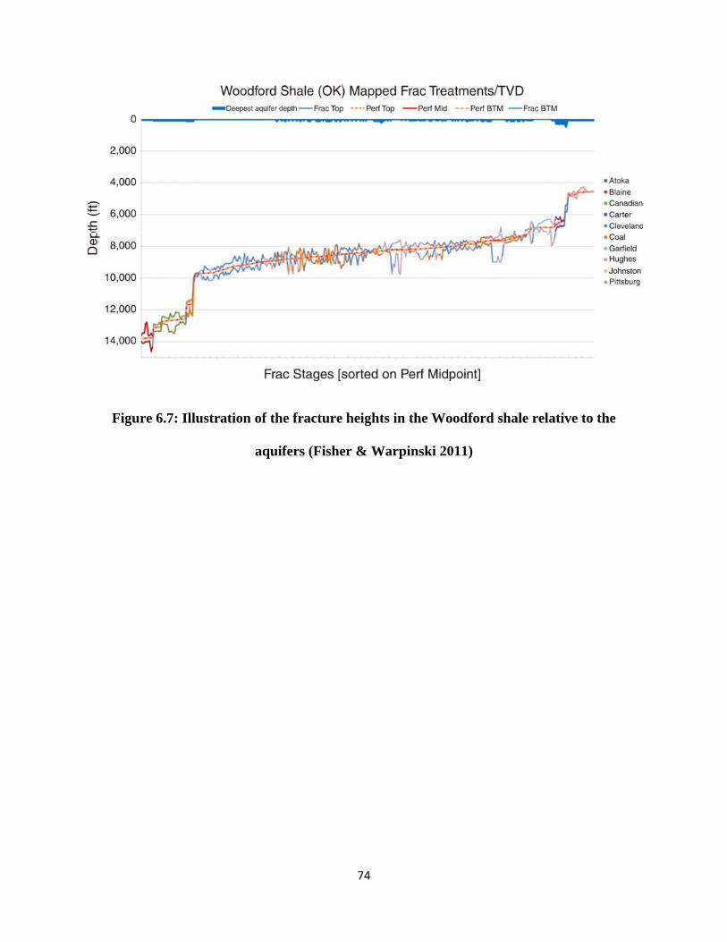
74

Figure 6.7: Illustration of the fracture heights in the Woodford shale relative to the

aquifers (Fisher & Warpinski 2011)

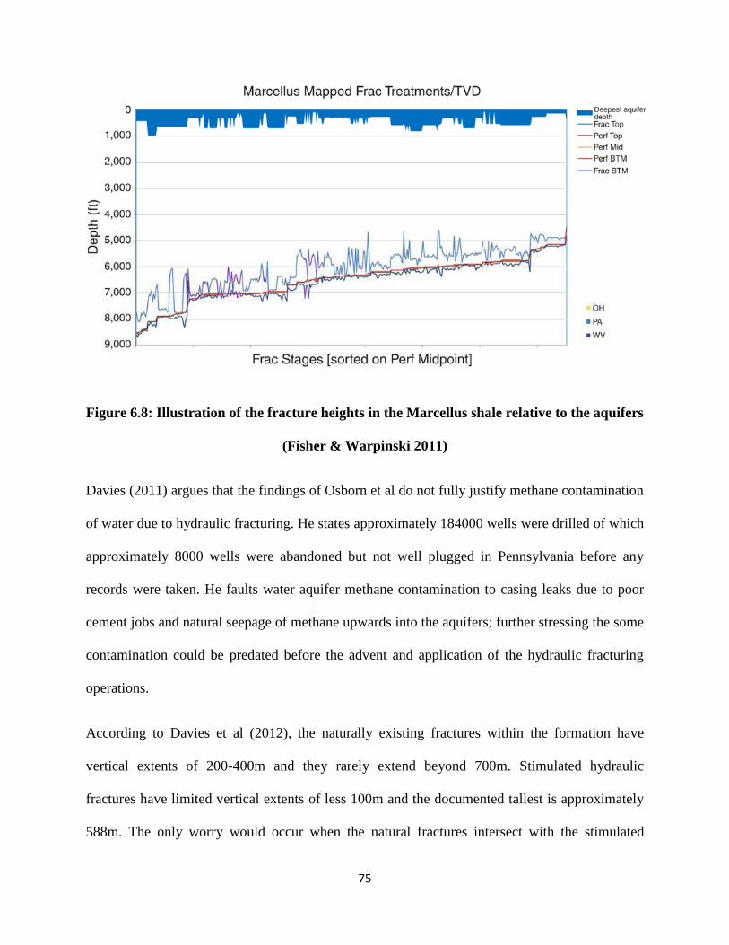
75

Figure 6.8: Illustration of the fracture heights in the Marcellus shale relative to the aquifers

(Fisher & Warpinski 2011)

Davies (2011) argues that the findings of Osborn et al do not fully justify methane contamination

of water due to hydraulic fracturing. He states approximately 184000 wells were drilled of which

approximately 8000 wells were abandoned but not well plugged in Pennsylvania before any

records were taken. He faults water aquifer methane contamination to casing leaks due to poor

cement jobs and natural seepage of methane upwards into the aquifers; further stressing the some

contamination could be predated before the advent and application of the hydraulic fracturing

operations.

According to Davies et al (2012), the naturally existing fractures within the formation have

vertical extents of 200-400m and they rarely extend beyond 700m. Stimulated hydraulic

fractures have limited vertical extents of less 100m and the documented tallest is approximately

588m. The only worry would occur when the natural fractures intersect with the stimulated

76

hydraulic fractures increasing the total vertical height extent which might communicate with the

aquifers.

6.3 CONCLUSION

As clearly indicated in the previous sections of this case study, underground water aquifer

contamination by the methane gas occurs under two valid circumstances; that is through casing

leaks or connection of the generated hydraulic fractures with the naturally existing fissures

increasing tremendously the vertical fracture height leading to the communication with the

underground shallow water aquifers.

In relation to the motive of this project report, my interest is in the water aquifer contamination

as a result of the generated hydraulic fractures connecting with the naturally existing fissures

(faults) extending the fracture height to the extent of contaminating the natural water aquifers. I

strongly believe that since the formation is composed of different rock strata of differing

properties plus the cap rock, this impedes the propagation of the fractures out of the pay zone.

The extensive distance between the aquifers and the payzones also act as an extra impediment to

the fracture propagation towards the water aquifers. In a different perspective basing on my

knowledge of petroleum geology, if the generated hydraulic fractures happened to connect with

the naturally existing fractures in the formation then methane gas can migrate upwards towards

the aquifers and the chances of this happening are one in a million

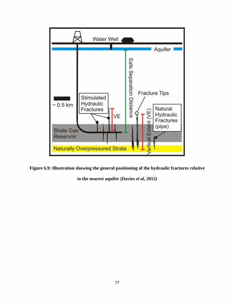
77

Figure 6.9: Illustration showing the general positioning of the hydraulic fractures relative

to the nearest aquifer (Davies et al, 2012)

78

REFERENCES

1. Michael J. Economides & Kenneth G. Nolte. (2000): Reservoir Stimulation; Third

Edition

2. John L. Gidley, Stephen A. Holditch, Dale E. Nierode and Ralph W. Veatch Jr. (1989) :

―Recent Advances in Hydraulic Fracturing‖ Monograph Vol 12 SPE Henry L. Doherty

Series, Richardson Texas

3. Carl T. Montgomery, Michael B. Smith (2010); ―Hydraulic fracturing – History of an

enduring technology‖

4. Andrew P. Bunger, John McLennan, Rob Jeffrey (2013); ―Effective and Sustainable

Hydraulic Fracturing‖ Intech

5. Ralph W. Veatch, Jr. (2008) ―A Historical Perspective of Hydraulic Fracturing‖

6. J.L Jensen, W.B. Ayers and T.A Blasingame (2003); Introduction to Shaly Sand Analysis

7. S.A. Holditch, B.M. Robinson, W.S. Whitehead (1987) Prefracture and Postfracture

Formation Evaluation Necessary To Characterize the Three Dimensional Shape of a

Hydraulic Fracture

8. Coretrack Limited (2013) website Accessed on 26/6/2013

http://www.coretrack.com.au/products-and-technology/the-coring-process

9. Coring and Core Analysis (Introduction) (2008) Retrieved from

http://petroleumcrudeoil.blogspot.ca/2008/11/coring-and-core-analysis-introduction.html

10. http://www.geomore.com/rock-cores/

11. A. Ali Daneshy, Daneshy Consultants International (2009) Factors Controlling the

Vertical Growth of Hydraulic Fractures

79

12. N.R. Warpinski, Sandia Natl. Labs; Z.A. Moschovidis, Amoco Production Co.; C.D.

Parker, Conoco Inc.; I.S. Abou-Sayed, Mobil E&P Technical Center(1994) Comparison

Study of Hydraulic Fracturing Models—Test Case: GRI Staged Field Experiment No. 3

(includes associated paper 28158 )

13. Kevin Fisher, Norm Warpinski (2011); ―Hydraulic Fracture Height Growth: Real Data‖

14. Simonson, E. R., Abou-Sayed, A. S., and Clifton, R. J. (1978): ―Containment of Massive

Hydraulic Fractures‖

15. Tushar Vatsa, John Yilin Wang (2011); ―Fracture Height Containment in the Stimulation

of Oriskany Formation‖

16. D. B. Larson, H. X. Nguyen (1984); ―Fracture Height Containment by Creating an

Artificial Barrier‖

17. Kamel Ben Naceur, Eric Touboul (1990); ―Mechanisms Controlling Fracture Height

Growth in Layered Media‖

18. Cleary, M. P.: ―Primary Factors Governing Hydraulic Fractures in Heterogeneous

Stratified Formations,‖ Paper ASME 78-Pet-47

19. Shuzhi Liu, Shuquan Ren, Jinzhou Zhao, Liangxian Yang, Qingxiang Wang, Shu Chen

(1998); ―The Fracturing Technique to Limit Hydraulic Fracture Height Growth Put into

Effect Successfully in Xinjiang Oil Field‖

20. Hanson A. W. and Lyons W. (1964); ―Method of Fracturing Formations‖

21. Hanson A. W. (1964); ―Plastically Deformable Solids in Treating Subterranean

Formations‖

80

22. Hemanta Mukherjee, B. F. Paoli, Todd McDonald, Hugo Cartaya and J. A. Anderson

(1995); ―Successful Control of Fracture Height Growth by Placement of Artificial

Barrier‖

23. Robert D. Baree‘ and Hermanta Mukherjee (1995); ―Design Guidelines for Artificial

Barrier Placement and Their Impact on Fracture Geometry‖

24. N. R. Warpinski and L. W. Teufel (1987); ―Influence of Geologic Discontinuities on

Hydraulic Fracture Propagation‖

25. Teufel, L. W. and Clark, J.A. (1984): ― Hydraulic Fracture Propagation in Layered Rock:

Experimental Studies Of Fracture Containment,‖

26. Anderson, G.D. (1981): ― Effects of Friction on Hydraulic Fracture Growth Near

Unbonded Interfaces in Rocks,‖

27. Mohammad Al-Dhamen, Areiyando Makmun, Ahmed Hilal (2013); ― Production

Optimization with Hydraulic fracturing: Application of Fluid Technology to Control

Fracture Height Growth in Deep Hard-Rock Formation‖

28. Warpinski, N. R., Branagan, P. T., Peterson, R.E., and Wolhart, S. L. (1998), ―An

Interpretation of M-Site Hydraulic Fracture Diagnostic Results‖

29. Barree, R. D., and Winterfeld, P.H. (1998), ―Effects of Shear Planes and Interfacial

Slippage on Fracture Growth and Treating Pressures‖

30. Norman R. Warpinski; ―Measurements and Observations of Fracture Height Growth‖

Halliburton 2011

31. Avner Vengosh, Nathaniel Warner, Rob Jackson, Tom Darrah; ―The effects of shale gas

exploration and hydraulic fracturing on the quality of water resources in the United

States‖

81

32. Richard J. Davies, Simon A. Mathias, Jennifer Moss, Steinar Hustoft, Leo Newport

(2012); ―Hydraulic Fractures How Far Can They Go?‖

33. James L. ―Chip‖ Northrup; ―How gas wells leak‖ (2011)

34. Stephen G. Osborn, Avner Vengosh, Nathaniel R. Warner, Robert B. Jackson (2011);

―Methane contamination of drinking water due to gas well drilling and hydraulic

fracturing.‖

35. Chris Mooney (2011); ―Truth about fracking‖

36. Norm R. Warpinski (2013); ―Understanding Hydraulic Fracture Growth, Effectiveness

and Safety through Microseismic Monitoring – Effective and Sustainable Hydraulic

Fracturing‖

37. Mark Zoback, Saya Kitasei, Bradford Copithorne (2010); ―Addressing the Environmental

Risks from Shale Gas Development‖

38. Richard J. Davies (2011); ―Methane contamination of drinking water caused by hydraulic

fracturing remains unproven‖

39. Amit D. Nakhwa, Ken Huggins, Ronald Sweatman. (2013); ―New Technologies in

Fracturing for Shale Gas Wells are Addressing Environmental issues.‖