applied sciences

Article

Control of a Robotic Swarm Formation to Track a DynamicTarget with Communication Constraints: Analysisand Simulation

Charles Coquet 1,2,* , Andreas Arnold 2,† and Pierre-Jean Bouvet 3,†

Citation: Coquet, C.; Arnold, A.;

Bouvet, P.-J. Control of a Robotic

Swarm Formation to Track a Dynamic

Target with Communication

Constraints: Analysis and Simulation.

Appl. Sci. 2021, 11, 3179.

https://doi.org/10.3390/app11073179

Academic Editor: Álvaro Gutiérrez

Received: 1 March 2021

Accepted: 25 March 2021

Published: 2 April 2021

Publisher’s Note: MDPI stays neutral

with regard to jurisdictional claims in

published maps and institutional affil-

iations.

Copyright: © 2021 by the authors.

Licensee MDPI, Basel, Switzerland.

This article is an open access article

distributed under the terms and

conditions of the Creative Commons

Attribution (CC BY) license (https://

creativecommons.org/licenses/by/

4.0/).

1 Institute of Movement Science, Aix Marseille University, CNRS, ISM, 13007 Marseille, France2 General Sonar Studies Department, Thales Defense Mission Systems, 29200 Brest, France;

andreas.arnold@fr.thalesgroup.com3 L@bISEN Yncréa Ouest, ISEN Brest, 29200 Brest, France; pierre-jean.bouvet@isen-ouest.yncrea.fr* Correspondence: charles.coquet.29200@gmail.com† These authors contributed equally to this work.

Abstract: We describe and analyze the Local Charged Particle Swarm Optimization (LCPSO) algo-rithm, that we designed to solve the problem of tracking a moving target releasing scalar informationin a constrained environment using a swarm of agents. This method is inspired by flocking algorithmsand the Particle Swarm Optimization (PSO) algorithm for function optimization. Four parametersdrive LCPSO—the number of agents; the inertia weight; the attraction/repulsion weight; and theinter-agent distance. Using APF (Artificial Potential Field), we provide a mathematical analysis ofthe LCPSO algorithm under some simplifying assumptions. First, the swarm will aggregate andattain a stable formation, whatever the initial conditions. Second, the swarm moves thanks to anattractor in the swarm, which serves as a guide for the other agents to head for the target. By focusingon a simple application of target tracking with communication constraints, we then remove thoseassumptions one by one. We show the algorithm is resilient to constraints on the communicationrange and the behavior of the target. Results on simulation confirm our theoretical analysis. Thisprovides useful guidelines to understand and control the LCPSO algorithm as a function of swarmcharacteristics as well as the nature of the target.

Keywords: PSO; OSL; tracking; flocking; swarm

1. Introduction

Controlling the collective behavior of a large number of robots is a complex task. How-ever, large natural multi-agent systems are known to work very well, such as bird flocks [1–3],fish schools [2,4,5], ants using pheromones [2,6], or aggregations of bacteria [2,7,8]. Theseself-organized systems have served as a source of inspiration to control large formationsof robots to prevent collisions between these robots [9]. The emergence principle wherecomplex collective behaviors arise from simple, elementary rules governing individuals isthe main topic of interest for artificial swarming systems. However, the emergence of swarmbehavior requires some constraints on the number of agents, the environment, and so forth.Also, it is difficult to design the elementary rules for a specific desired collective behaviorto emerge.

One behavior in particular, flocking or schooling, enjoys a growing interest in thescientific domain. Ref. [10] established a first landmark, giving the three rules of flocking(alignment, cohesion, separation). Then Tanner, Jadbabaie and Pappas, in a two-partarticle [11,12], made a fundamental mathematical analysis of the Reynolds rules usingthe Artificial Potential Field (APF) approach. They proved that using potentials bothattractive and repulsive, the flock becomes homogeneous with equal inter-agent distanceand equal speed vectors at equilibrium. This behavior is resilient to external stimuli as longas the agents are within communication range. By using these methods, and despite the

Appl. Sci. 2021, 11, 3179. https://doi.org/10.3390/app11073179 https://www.mdpi.com/journal/applsci

Appl. Sci. 2021, 11, 3179 2 of 21

remaining challenges to designing the desired group behavior, the robotics community hasused swarm-based approaches for applications such as target tracking [13–17], Search AndRescue (SAR) [18], or Odor Source Localization (OSL) [19–26], among others.

Ant Colony Optimization (ACO) [6] or Particle Swarm Optimization (PSO) [27] areswarm intelligence algorithms used in the mathematical community of optimization. Thestrength of these approaches lies in using agents distributed in the workspace, sharinginformation to search for the optimum of a fitness function. In particular, this communitystrongly uses the PSO algorithm [13–15,18–21,28]. It is important to stress that optimizationalgorithms like PSO, can also drive a swarm of actual robots [29]. This bridge between thetwo communities of robotics and optimization shows that one common way to solve theirrespective problems can be found through swarming.

In the present paper, we focus on tracking a mobile target leaving a semi-permanenttrail, such as a chemical scent or radioactive particles carried by the environment. Thisproblem could be described as Mobile Odor Source Localization (MOSL), a generalizationof OSL. We assume the information to be “scalar”, in that its value is a real, one-dimensionalnumber. As Section 2 will show, this problem is equivalent to maximizing a fitness functionvarying with space and time. The plume model is simplified compared to the state-of-the-art [30,31] to fasten the simulation results and obtain preliminary results but thosemodels will be upgraded in a future work. In a terrestrial environment, instances of thisproblem arise for example, when tracking a moving source of nuclear radiation withpossible counter-terrorist applications [32,33], or finding the origin of polluted areas [34].Applications in the marine field include securing a specified area to detect intruders; toprevent illegal oil discharges by ships using so-called “magic pipes”; localizing a pipelineleak [35,36], or various other similar uses. A variant of PSO called Charged Particle SwarmOptimization (CPSO) was proposed by [20,21] to solve OSL and head for a static odorsource, with interesting results [37]. CPSO differs from PSO in that repulsive componentsare added to avoid collisions between agents in the swarm. The equations of flocking corre-late with CPSO [38,39], or more recently with the Extended PSO [28], but no mathematicalanalysis has yet linked up those two fields.

In [40], for our MOSL problem, we proposed an algorithm called LCPSO, inspired byCPSO, which takes into account communication constraints in distance between agentsthat are representative of underwater systems [41]. Based on simulations, we showedthat the limited number of attracting agents allows a reactive tracking of one or multiplemoving targets avoiding collisions between agents, with better performances than the CPSOalgorithm. In this paper, we intend to demonstrate new results characterizing LCPSO.First, we demonstrate that the positions of the center of gravity and attractor(s) will guidethe swarm, and this mechanism is the key to head for the source. Second, we show thata distance parameter, req, which is an input of our algorithm, can control the surface ofthe swarm. Finally, we show that, whatever the initial conditions, the swarm will attain astable formation, invariant to time and the place of the attractor. We prove these resultstheoretically under some simplifying hypotheses, whatever the dimension D. We thensuccessively remove the simplifying hypotheses and show that the proposed theoreticalresults are confirmed by simulations. These flocking behaviors have already been shownin [12,39]. However, to the best of our knowledge, controlling the surface of the swarm withan optimization algorithm such as PSO and its derivatives is new. Also, the use of specificattractors to head for a goal indirectly and in the same time keeping a strong formation,has never been investigated before, to the best of our knowledge.

We organize our article as follows. Section 2 formalizes the MOSL problem whileSection 3 describes our models, particularly the PSO algorithm and the LCPSO algorithm totrack a mobile target. New contributions begin at Section 4, which provides a mathematicalanalysis of the behavior of the LCPSO algorithm under some restricting hypotheses. Thosehypotheses are removed one by one to show that our algorithm is resilient to a limitedcommunication range. Section 5 provides simulations results of our algorithm in mobile

Appl. Sci. 2021, 11, 3179 3 of 21

target tracking scenario. Finally, Section 6 concludes this paper and gives some perspectivesfor future works.

2. Problem Formulation2.1. The General MOSL Problem

We extend the OSL problem, where the odor source is static, to the case of movingsource resulting in the MOSL problem. The objective is to localize a mobile target, charac-terized by a D-dimensional position ps(t) varying with time t. This target is assumed torelease scalar information in the environment, such as an odor, heat, radioactivity, a soundor radio wave; without losing generality we assume the intensity of this information tobe positive. We thus note u : RD × R 7→ R+; (p, t) → u(p, t). This information u isassumed to be diffused and transported by the environment. This can be modeled by a partialdifferential equation of variable u, which exact formulation depends on the problem at hand.We assume furthermore that at any given time t, function u has an unique point pmax(t)where the information intensity u is maximum. We also assume that the diffusion andtransport mechanism is such that pmax(t) is very close to the position of the target ps(t)so that for all practical purposes we may assume that ps(t) ≈ pmax(t), that is, both termscan be used interchangeably. Our problem is then to find pmax(t), which is then equivalentto finding the position of the target at the same date. Another thematic close to MOSL isgeofencing [42] where Unmanned Aerial Vehicles (UAV) can be used in a constrained area,typically cities, for tracking and tracing missions, as for the track of stolen cars.

The measure, made by the system’s sensors, will be denoted by function f : RD×R 7→R+; (p, t)→ u(p, t) + β(p, t), where β(p, t) is a noise. We assume that the Signal-to-noiseRatio (SNR) is sufficient so that the maximum of f still coincides with the maximum of ufor all practical purposes. In our simulations, we considered that function u had values in[0, 1] and the noise was additive white Gaussian, uncorrelated in space and time, with astandard deviation σ taken between 0 and 0.25 except where indicated. We leave issuesraised by a poor SNR for future research.

2.2. The Toy Problem Used in This Paper

Instead of describing the problem by a partial derivative equation, we may insteadassume that the solution of this equation is known explicitly. This is the approach we usein the simulations presented in this paper because this is quicker to simulate. We use forinstance the following expression:

u(p, t + ∆t) =1

1 + ‖p− ps(t)‖2︸ ︷︷ ︸1

+ (1− e−∆tτ )u(p, t)︸ ︷︷ ︸2

f (p, t) = u(p, t) + β(p, t)︸ ︷︷ ︸3

.(1)

In these equations, ∆t is a discrete time step. The Equation (1) contains three elementsto represent real-world phenomena:

1. a spatial term which decreases with the distance between target position ps and anyposition p in the workspace; this is the inverse square law induced by mechanisms ofconservation of power through propagation, modified with a constant additive termin the denominator to prevent the value from becoming unreasonably large when‖p− ps(t)‖ → 0;

2. a temporal term, representing a decay, inspired by the response to a first-order filtermodel parameterized by the time constant τ;

3. an additive white Gaussian noise β(p, t) ∼ N (0, σ) in the whole environment, withσmax( f ), representing measurement noise.

In our paper, dimension D can be 1 or 2 or more, and it will be indicated explicitlywhen it is necessary. Simulation results are not treated in higher dimensions, but we

Appl. Sci. 2021, 11, 3179 4 of 21

assume that the results we present should be close to the results displayed in Dimension 2because there are no cross-dimensional terms in the PSO equation described below inExpression (2).

We must stress that the exact mechanism behind the generation of function u doesnot need to be known for the problem to be solved. The only hypotheses that matter,are that (i) there is only one spatial maximum for u at each date and (ii) that the maximumis reached close to the actual position of the target at a given date. This way, all that mattersis finding the maximum of u at each date by sampling f at the positions of the agents inthe swarm.

This model is less complex that in the state-of-the-art [31,37,43], where the plumemodel is dynamic and with multiple local maxima. Environmental sensors help the modeli-sation of this plume, an anemometer or ocean current sensor for example. However, in OSL,the source is static, and the important point we wanted to highlight is the unpredictabilityof the source behavior. Hence, study our algorithm with both the plume and source dy-namics will complicate the analysis of our algorithm. For this reason, the analysis takesinto account only the dynamics of the source, and an analysis with a dynamic plume modelwill be part of a future work. We note that the measurement noise can create multiple localmaxima, but this phenomenon can disappear instantaneously at the next time step for theagent i.

3. Models3.1. The PSO Algorithm

PSO is an evolutionary algorithm, inspired by flocking birds [27]. We consider Ntrackers sampling f at their position pi(t). This value is given by f

(pi(t), t

)from (1). The

trackers move to maximise f (pi(t), t). To do this, the PSO algorithm provides an update ofthe speed vector vi(t) as follows:

vi(t + ∆t) = c0vi(t)︸ ︷︷ ︸1

+ c1αi1(t)(pb

i (t)− pi(t))︸ ︷︷ ︸

2

+ c2αi2(t)(pg(t)− pi(t)

)︸ ︷︷ ︸3

. (2)

As described in (2), the speed vector at time t + ∆t is a sum of three elements:

1. The previous speed vector of tracker vi(t), weighted by a constant coefficient c0.For the convergence of the algorithm, we need to have c0 ∈]− 1; 1[ [44]. c0 is homoge-neous to a (pseudo) mass and is sometimes called “inertia” in the community.

2. The difference between the current position of tracker i and its best historical positionnoted pb

i (t) ( “b” for “best”). The best historical position pbi (t) is the position pi(ti),

with ti between time 0 and t where measure f (pi, ti) was the greatest. This componentis weighted by a constant coefficient c1.

3. The difference between the position pg(t) (“g” for “global”) of the current swarm’sbest tracker and the current position of tracker i. The position of the best tracker ofswarm pg(t) is the tracker j measuring the greatest f (pj, t) among the N trackers ofthe swarm. This component is weighted by a constant coefficient c2.

The second and last components are attractors, weighted by a random number, respec-tively αi1(t) and αi2(t), uniformly distributed in [0, 1] and specific to agent i. These randomnumbers provide diversity to the system and improve exploration, avoiding the swarm tobe trapped in a local optimum [27,45].

Using the Euler integration scheme, the updated position of tracker i is computed asthe sum of its previous position and the updated speed vector as follows [27]:

pi(t + ∆t) = pi(t) + ∆t · vi(t + ∆t). (3)

3.2. APF Theory and Flocking Principles

In APF methods, the analysis is based on potential functions P(di,j(t)

), where di,j(t) =∥∥pi(t)− pj(t)

∥∥ is the Euclidean distance between agents i and j. The agent i uses a gradient

Appl. Sci. 2021, 11, 3179 5 of 21

descent algorithm based on P(di,j(t)

)to move. In flocking algorithms, we are interested in

a particular potential function P(di,j(t)

), described in Definition 1.

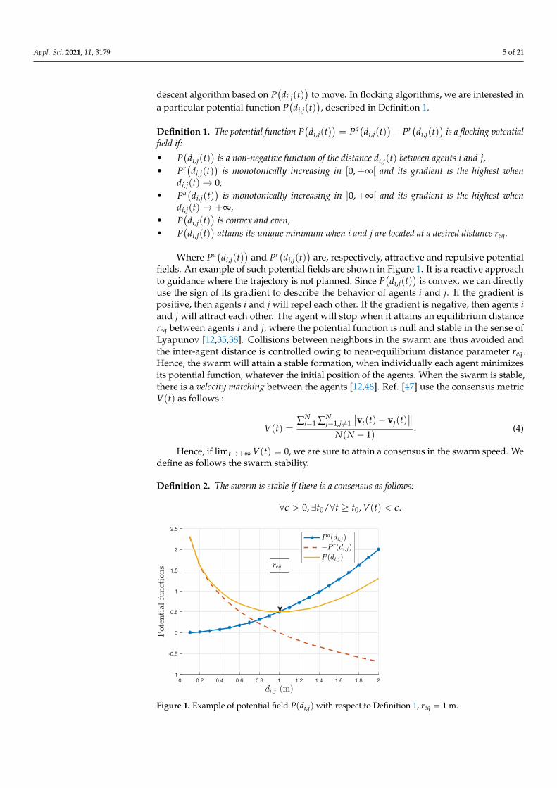
Definition 1. The potential function P(di,j(t)

)= Pa(di,j(t)

)− Pr(di,j(t)

)is a flocking potential

field if:

• P(di,j(t)

)is a non-negative function of the distance di,j(t) between agents i and j,

• Pr(di,j(t))

is monotonically increasing in [0,+∞[ and its gradient is the highest whendi,j(t)→ 0,

• Pa(di,j(t))

is monotonically increasing in ]0,+∞[ and its gradient is the highest whendi,j(t)→ +∞,

• P(di,j(t)

)is convex and even,

• P(di,j(t)

)attains its unique minimum when i and j are located at a desired distance req.

Where Pa(di,j(t))

and Pr(di,j(t))

are, respectively, attractive and repulsive potentialfields. An example of such potential fields are shown in Figure 1. It is a reactive approachto guidance where the trajectory is not planned. Since P

(di,j(t)

)is convex, we can directly

use the sign of its gradient to describe the behavior of agents i and j. If the gradient ispositive, then agents i and j will repel each other. If the gradient is negative, then agents iand j will attract each other. The agent will stop when it attains an equilibrium distancereq between agents i and j, where the potential function is null and stable in the sense ofLyapunov [12,35,38]. Collisions between neighbors in the swarm are thus avoided andthe inter-agent distance is controlled owing to near-equilibrium distance parameter req.Hence, the swarm will attain a stable formation, when individually each agent minimizesits potential function, whatever the initial position of the agents. When the swarm is stable,there is a velocity matching between the agents [12,46]. Ref. [47] use the consensus metricV(t) as follows :

V(t) =∑N

i=1 ∑Nj=1,j 6=1

∥∥vi(t)− vj(t)∥∥

N(N − 1). (4)

Hence, if limt→+∞ V(t) = 0, we are sure to attain a consensus in the swarm speed. Wedefine as follows the swarm stability.

Definition 2. The swarm is stable if there is a consensus as follows:

∀ε > 0, ∃t0/∀t ≥ t0, V(t) < ε.

0 0.2 0.4 0.6 0.8 1 1.2 1.4 1.6 1.8 2

-1

-0.5

0

0.5

1

1.5

2

2.5

Figure 1. Example of potential field P(di,j) with respect to Definition 1, req = 1 m.

Appl. Sci. 2021, 11, 3179 6 of 21

3.3. PSO Formulated Using the APF Theory

As we have introduced APF theory and flocking principles, we can now rewrite thePSO Equation (2) as a gradient descent strategy:

vi(t + ∆t) = c0vi(t)−∇pi Pi(t). (5)

Here, Pi(t) is the potential field of PSO applied to agent i, providing equality ofEquations (2) and (5). Since potential fields use only phenomena of attraction/repulsionwith inter-agent distance, weight c0 does not appear in potential field Pi(t). So we find:

Pi(t) = Pa(∥∥∥pbi (t)− pi(t)

∥∥∥)+ Pa(‖pg(t)− pi(t)‖)

=c1αi1(t)

2

∥∥∥pbi (t)− pi(t)

∥∥∥2+

c2αi2(t)2‖pg(t)− pi(t)‖2. (6)

Here, Pa(di,j(t))

is a generic potential attraction field known in APF literature as aquadratic attractor [48]:

Pa(di,j(t))= A · d2

i,j(t), (7)

where A is a random number uniformly distributed in [0, c12 ] and [0, c2

2 ] respectively. Hence,when the algorithm converges, all the agents will be located at the same position. So, toapply this algorithm to robotics, we need to include repulsive mechanisms to be coherentwith Definition 1.

3.4. The LCPSO Algorithm3.4.1. Adding an Anti-Collision Behavior to PSO: CPSO

The objective here is to determine a potential field Pi(t), inspired by PSO potential (6),that meets Definition 1. To do this, Ref. [20] introduced a variation of PSO, called CPSO,which was demonstrated experimentally with interesting results [20,37]. To derive theequations of CPSO, we define the following unbounded repulsive potential [39]:

Pr(di,j(t))= log

(di,j(t)

). (8)

This potential verifies that Pr(di,j(t))→ −∞ when di,j(t)→ 0. If we sum the attractivepotential (7) and the repulsive one (8), we obtain a potential that meets Definition 1.

Those models of potentials are not unique. The state of the art provides good examplesof possible potential functions for flocking algorithms [38,39]. However, for the analysis atequilibrium, we need the attractive potential defined in (7) for two reasons. First, we keepthe links with the original PSO algorithm. Second, this particular model is necessary forsome theorems, Theorem 4 in particular, which is important to determine the characteristicsof our swarm formation.

The repulsive potential is then added to the PSO equation:

vi(t + ∆t) =c0vi(t) + c1αi1(t)(

pbi (t)− pi(t)

)(9)

+ c2αi2(t)(

pg(t)− pi(t))− c3

N

∑j=1,j 6=i

∇pi Pr(di,j(t)

),

where c3 is the constant repulsive weight between trackers i and j.

3.4.2. LCPSO, a CPSO Variant to Deal with Some Real-World Constraints

First, to reflect limitations in communication links, a local communication constraintis added to the model. Indeed, the best tracker position of the swarm pg(t) in Equation (9)is global, shared with each agent of the swarm. We use the local-best vector position pl

i(t)(l for local), which is the position of tracker j in the neighborhood set of i where measure

Appl. Sci. 2021, 11, 3179 7 of 21

f (pj, t) is the greatest. The neighborhood set Ni(t) is based on parameter rcom whichdenotes the maximum communication range between tracker i and its neighbors [12].Beyond maximum communication range rcom data transmission is impossible, below rcomtransmission is perfect :

Ni(t) = j|∥∥pi(t)− pj(t)

∥∥ < rcom, i 6= j ⊂ 1, · · · , N. (10)

This decentralization was already proposed by [14,15] but to the best of our knowledgeit was never used in the aim of mobile target tracking. Each vehicle will have its own localbest position and will move towards its best neighbor.

Second, the best historical position pbi (t) is removed in the proposed approach. This

is because the target is not static: it changes position with time.Finally, to obtain a stable swarm formation, we set our random component αi2(t) to 1.

The analysis of the algorithm with random components can be the object of future work.Those considerations lead to the following model, originally introduced in [40], and whichwe named LCPSO:

vi(t + ∆t) =c0vi(t) + c2(pl

i(t)− pi(t))− c3 ∑

j∈Ni(t)∇pi P

r(di,j(t)). (11)

From Equation (11), we can deduce the potential function of LCPSO as follows:

Pi(t) = Pa(∥∥∥pli(t)− pi(t)

∥∥∥)− ∑j∈Ni(t)

Pr(di,j(t))

(12)

This potential meets Definition 1, and is illustrated in Figure 1, with the correspondingattractive (7) and repulsive potentials (8) used for the LCPSO. The Euler integration schemeis the same as in Equation (3).

4. Analysis of the Properties of LCPSO4.1. Metrics and Hypothesis

While we already illustrated the behavior of the LCPSO algorithm earlier throughsimulation [40], these properties were only shown intuitively. We now wish to give somemathematical basis to this intuition. We make the following assumptions that will be validthroughout the mathematical analysis of this section:

• Communication range is unlimited. As a result, the local-best attractor pli(t) is the

best tracker position of the swarm pg(t).• We focus our efforts on the APF analysis, and to ease the analysis we set c0 to 0. So the

speed vector vi(t + ∆t) is updated only with the gradient descent of the potentialfield equation.

• The target’s behavior is not known from the swarm’s point of view and can bedynamic. Tracker i measures f (pi, t) and adjusts its local-best position pl

i(t) as afunction of maximum measurement of the neighborhood. Since the communicationrange is small, we make the hypothesis that information exchange is instantaneousbetween the trackers and is limited to their position in absolute coordinates and theirmeasurements, without noise.

To illustrate the inter-agent distance between nearest neighbors in the swarm, we intro-duce a new function, the swarm spacing ρ(N). We normalize this spacing by req, a parameterallowing us to control the inter-agent equilibrium distance when the swarm is stable, andthe number of agents N :

ρ(N) =1

req · NN

∑i=1

mini 6=j

di,j. (13)

Another important parameter is the surface area taken up by the swarm. For somecases, this parameter is critical to have a good tracking of the source. As we will see in

Appl. Sci. 2021, 11, 3179 8 of 21

Section 4.2, swarm formations have a convex hull inside a ball, and we will thus be able torepresent this surface with only one parameter, the radius of this ball rmax. Whatever thedimension, we have:

rmax = maxi∈[1,··· ,N]

‖p− pi‖req

. (14)

With p the center of gravity of our swarm, represented by the following equation:

p(t) =1N

N

∑i=1

pi(t). (15)

Our swarm model has a lot of mathematical similarities with the models of [39].So, for conciseness, the demonstrations too close from [39] are not given, and the otherones are in the Appendix A. Moreover, all the theorems presented in this paper are trueregardless of the repulsive potential Pr(di,j), as long as it respects Definition 1. Thus,we could imagine that, if the repellent potential is not suitable, we could test others thatexist in the state of the art [38,39].

4.2. Behavior of LCPSO

We suppose that the agents’ positions are taken in RD, with D the dimension. S(t)is the set of agents’ positions pi(t) of the swarm at time t, i ∈ [1, · · · , N]. Let us noteC(t) as a convex hull of S(t): it is a continuous subset of RD. Then let us note C(t)as the convex polygon of S(t). It is a manifold of dimension D − 1 which displays thesurface taken by the swarm. We set y(t) ∈ RD the optimum position of f at date t:y(t) = arg maxy f (y, t). We suppose that this optimum is unique and is the position of thetarget ps(t) propagating information.

We define the set B(t), which contains the best attractors of the swarm at time t whichminimised the Euclidean distance with respect to y(t).

B(t) = p(t) ∈ RD|p(t) = arg minp(t)∈S(t)

‖p(t)− y(t)‖. (16)

The set S(t) being discrete, we introduce the set S(t), defined as the set of the pointsof S(t) which are in the convex polygon C(t) of S(t). We summarize the behavior of ourswarm with the following theorem:

Theorem 1. We assume that each agent follows the LCPSO Equation (11), with rcom → +∞.Then the center of gravity of the swarm is heading towards the attractor pg(t), and its velocityvector is equal to :

v(t + ∆t) = c0v(t) + c2(pg(t)− p(t)

). (17)

Hence, if the swarm is stable in the sense of Definition 2, all agents follow the speedvector of the center of gravity. Taking into account the inertia weighted by c0, the attractorposition gives the direction that the swarm will follow. In the MOSL case, we have definedit as the agent that has measured the strongest information f (pg, t) at time t; it is thus theagent that is the closest to the target.

We distinguish two particular states. The first one is the transition state, with y(t) /∈C(t). In this state, the attractors are necessarily and intuitively the agents located on thehull of the swarm: B(t) ⊆ S(t). Trying to catch up with these attractors, the agents inthe swarm will accelerate to their maximum speed and then remain at this speed, in asteady state. Thanks to (17) and rmax, the maximal speed vmax is predictable. This state isillustrated in Figure 2b in dimension 2. The second case is the steady state, with y(t) ∈ C(t).In this state, all agents of S(t) are potentially attractive, that is, B(t) ⊆ S(t). In this case,the swarm will follow a speed close to that of the target. Thus, the closer the attractor is tothe center of gravity, the slower its speed will be. In the case of tracking a static target, our

Appl. Sci. 2021, 11, 3179 9 of 21

swarm will head towards the source, and will stop when y(t) = p(t), shown in Figure 2ain Dimension 2.

𝐲(𝑡)

, , = 𝑆(𝑡)

, = ҧ𝑆 (𝑡)

= ത𝐵(𝑡)

= 𝐶(𝑡)

= ҧ𝐶(𝑡)

𝐲(𝑡)𝑟𝑚𝑎𝑥

= 𝐯𝑖(𝑡 + Δ𝑡)

(a) (b)

Figure 2. Possible states for the swarm; the target is in red. (a) Steady state; (b) Transition state.

4.3. Analysis with N = 2 Agents

We consider, without loss of generality, that the attractor is agent 1. The potentialfunctions derived from (12) becomes:

P1(t) = −c3Pr1(d1,2(t)

)P2(t) =

c2

2Pa

2(d2,1(t)

)− c3Pr

2(d2,1(t)

).

We can see that the potential functions P1(t) and P2(t) are only dependent on inter-agent distance d1,2(t). We deduce the following theorem:

Theorem 2. A swarm of N = 2 agents following the potential field P(t) = P1(t) + P2(t) in a

gradient descent strategy will converge to an inter-agent distance at equilibrium req =√

2c3c2

.

To use req as a parameter in our algorithm, we will replace our parameter c3 by an

expression including the so-called equilibrium distance req. To do this, we set c3 =c2·r2

eq2 .

In dimension D, the LCPSO algorithm can then be rewritten as follows:

vi(t + ∆t) = c0vi(t) + c2

(pl

i(t)− pi(t)−r2

eq

2

N

∑j=1,j 6=i

∇pi Pr(di,j(t)

)). (18)

4.4. Swarm Stability

Theorem 3. We consider a swarm of agents following Equation (18), with potential functionsrespecting Definition 1. For any p(0) ∈ RND, as t→ +∞, we have p(t)→ Ωe.

With the vector p(t) which contains all the relative positions of the individuals inthe swarm and Ωe the invariant equilibrium set of the swarm; they are detailed in theAppendix A, with the proof. Hence, agents following (18) are going to reach stability inthe sense of Definition 2. If this Theorem is similar to the Theorem 1 of [39], the proof isdifferent because the LCPSO Equation (18) is not stationnary.

4.5. Symmetry and Robustness of the Swarm Formation

Due to the nature of the potential functions Pa(di,j) and Pr(di,j), their gradient is odd.Consequently, there is a reciprocity of the interactions between agents, with respect to theorigin [39]. These reciprocal interactions will naturally lead the swarm to have a symmetricalformation with respect to the center of gravity of the swarm p when it is stable in the senseof Definition 2 [39].

Appl. Sci. 2021, 11, 3179 10 of 21

Contrary to the swarm models detailed in [38,39], all interactions are not bidirectionalwhen looking at the whole system. Indeed, if this is true for interactions of repulsion,attraction relationships are unidirectional and directed towards the attractor. One couldtherefore assume that a change of attractor influences the strength of the formation when itis stable in the sense of Definition 1. However, with the LCPSO Equation (18), the formationis robust to this, regardless of the dimension D.

Theorem 4. By assuming N ≥ 2 agents using the flocking speed vector described in (18), whateverthe attractor pg(t), the equilibrium distance of agent i with the other agents will always be the same.

The proof is in the Appendix A. With the help of Theorem 2 from [39], we can see thatthe formation is bounded whatever the dimension D:

Theorem 5. If the agents follow the LCPSO Equation (18), as time progresses, all the members ofthe swarm will converge to a hyperball:

Bε(p) = p : ‖p− p‖ ≤ ε where ε =reqN

2

The proof is not present in this paper, because it is too similar to that of Theorem 2from [39]. ε increases linearly as a function of N in Theorem 5. We can see in Figure 3bthat the evolution of rmax as a function of N, in Dimension 1 or 2, does not have a linearevolution, but tends to “flatten” when N increases: thus, this bound is real, but not adaptedto approach the size of the swarm in reality.

Now, we will look more prospectively at the properties of the stable formation. We thuspresent conjectures, supported by simulation results, which will remain to be provenmathematically afterwards. We do not display results in Dimension 3, because the remarkswould be redundant with those in Dimension 2. We use rmax and ρ(N) to illustrate theevolution of the stable formations when N increases, depending on the dimension. Theresults are shown in Figure 3. In dimension 1, the formation of the agents when the swarmis stable in the sense of Definition 2 is unique, so we do not need several samples. In higherdimension, the multiplicity of emergent formations as a function of N lead up to severalpossible formations.

In dimension 1, we can see in Figure 3a that the more N increases, the more theswarm spacing ρ(N) decreases; this is rather logical, because the surface taken by theswarm widens very quickly, as we can see in Figure 3b. Hence, the more N increases, themore certain agents are distant from the attractor, the more the attraction strength is high,the more the swarm is compact.

In Dimension 2, when N = 3, the equilibrium formation is an equilateral triangle.When N is higher, the possible formations approach a circle whose the center of gravitydetermines a point of symmetry in the interactions between agents. This formation presentsone or several layers where the position of the agents is aligned on circles, and it becomesmore difficult to predict it, as shown in Figure 3f, with 2 layers for N = 15 agents. Moreover,in Figure 3b, we have 1 ≤ ρ(N) ≤ 1.3 whatever N and our samples: our parameter req isa good representation of swarm spacing. Since there is multiple neighbors, the repulsivepotential energy of an agent i is much higher than in dimension 1, and consequently theswarm spacing ρ(N) is higher in higher dimension. In Figure 3b, we can see that the radiusof the ball containing all the agents rmax varies very few with the samples. Hence, theswarm surface is predictable with few uncertainties.

Appl. Sci. 2021, 11, 3179 11 of 21

0 5 10 15 20 25 30 35 40 45 50

0.2

0.3

0.4

0.5

0.6

0.7

0.8

0.9

1

1.1

5 10 15 20 25 30 35 40 45

1

2

3

4

5

6

7

8

9

-250 -200 -150 -100 -50 0 50

-200

-150

-100

-50

0

50

(a) (b) (c)

2 5 8 11 14 17 20 23 26 29 32 35 38 41 44 47 50

1

1.05

1.1

1.15

1.2

1.25

2 5 8 11 14 17 20 23 26 29 32 35 38 41 44 47 50

0.5

1

1.5

2

2.5

3

3.5

4

4.5

-250 -240 -230 -220 -210

-205

-200

-195

-190

-185

-180

-175

-170

-165

-160

-155

(d) (e) (f)

Figure 3. Swarm evolution and formation following the Local Charged Particle Swarm Optimization (LCPSO) Equation (18).req = 7 m, c0 = 0, c2 = 0.5. (a) ρ(N) in dimension 1; (b) Radius rmax in dimension 1 and 2; (c) Example of swarm trajectory;(d) ρ(N) in dimension 2. Boxplots with 1000 samples; (e) rmax in dimension 2. Boxplots with 1000 samples; (f) Example ofemergent swarm formation.

4.6. Removing the Simplifying Hypotheses4.6.1. Non-Zero Mass c0

In a real robot, the weight c0 must be taken into account and is set according to itsgeometry and mass. This parameter will influence the speed norm of the agents whenthe formation is stable according to Definition 2. To illustrate our point, we keep thehypothesis that the attractor pg is always the same agent. Thanks to Theorem 1, we haveveq = −c2

(p(t)− pg(t)

)when c0 = 0. veq is invariant in time because the swarm formation

is stable. When c0 6= 0, we have:

v(t + ∆t) =c0 · v(t)− c2(p(t)− pg(t)

)=c0 ·

(c0 · v(t− ∆t)− c2

(p(t− ∆t)− pg(t− ∆t)

))+ veq

=veq ·tmax

∆t

∑k=0

ck0 =

tmax→+∞

veq

1− c0. (19)

Hence, if c0 influences the speed norm of the swarm, it does not influence its direction,which depends only on the position of the attractor. If the mathematical analysis is notimpacted by the pseudo-mass when |c0| < 1 [39,44], the pseudo-mass c0 greatly influencesthe convergence time of the swarm during its transitory phase, since it smoothes thetrajectory of the agents by taking into account the previous velocity vector.

We support what we have just said by Monte-Carlo simulations as a function of c0 inFigure 4, for N = 7 and N = 15 agents in dimension 2. For N = 7, the agents are distributedon the same circle around the center of gravity, while for N = 15, we have a distributionon 2 levels, as in Figure 3f. As our simulation time is tmax = 100 s, a convergence time

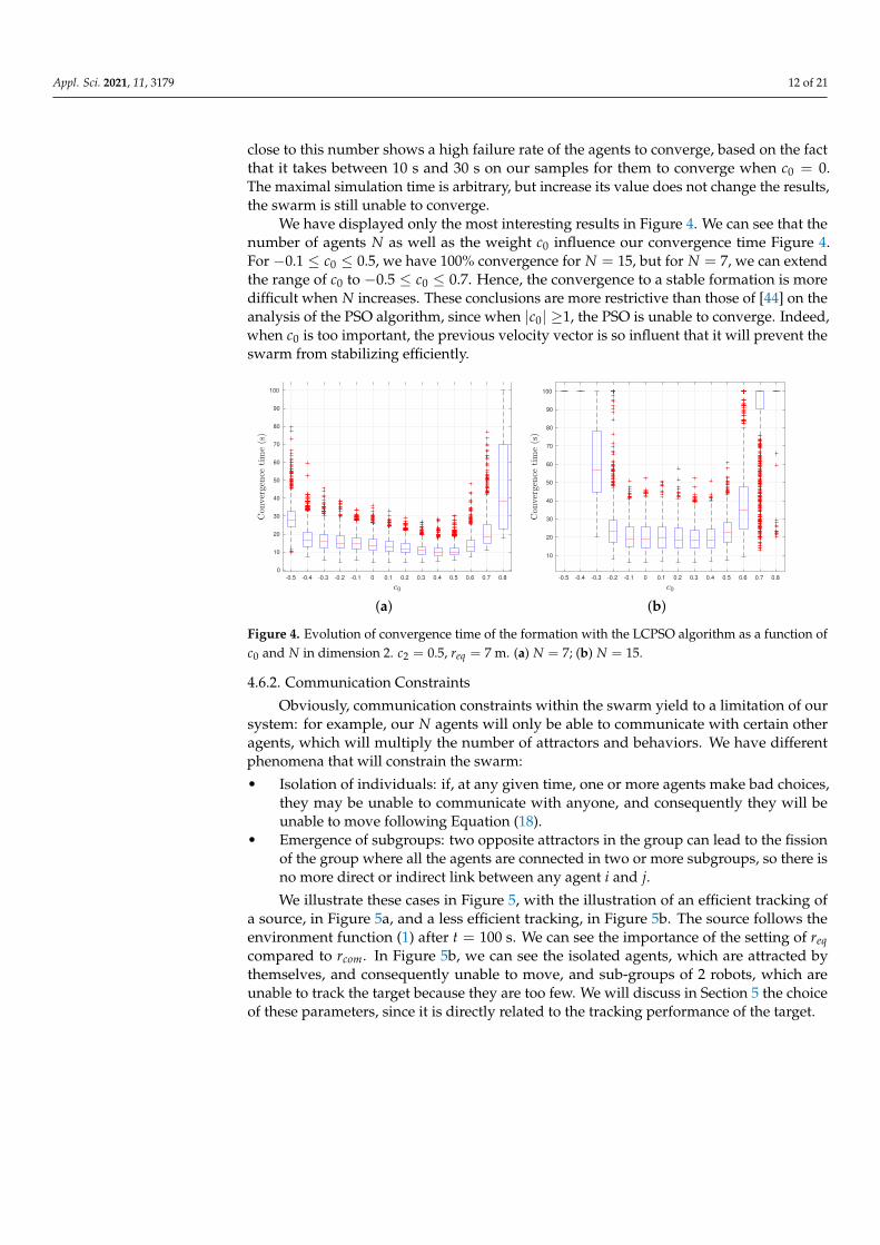
Appl. Sci. 2021, 11, 3179 12 of 21

close to this number shows a high failure rate of the agents to converge, based on the factthat it takes between 10 s and 30 s on our samples for them to converge when c0 = 0.The maximal simulation time is arbitrary, but increase its value does not change the results,the swarm is still unable to converge.

We have displayed only the most interesting results in Figure 4. We can see that thenumber of agents N as well as the weight c0 influence our convergence time Figure 4.For −0.1 ≤ c0 ≤ 0.5, we have 100% convergence for N = 15, but for N = 7, we can extendthe range of c0 to −0.5 ≤ c0 ≤ 0.7. Hence, the convergence to a stable formation is moredifficult when N increases. These conclusions are more restrictive than those of [44] on theanalysis of the PSO algorithm, since when |c0| ≥1, the PSO is unable to converge. Indeed,when c0 is too important, the previous velocity vector is so influent that it will prevent theswarm from stabilizing efficiently.

-0.5 -0.4 -0.3 -0.2 -0.1 0 0.1 0.2 0.3 0.4 0.5 0.6 0.7 0.8

0

10

20

30

40

50

60

70

80

90

100

-0.5 -0.4 -0.3 -0.2 -0.1 0 0.1 0.2 0.3 0.4 0.5 0.6 0.7 0.8

10

20

30

40

50

60

70

80

90

100

(a) (b)

Figure 4. Evolution of convergence time of the formation with the LCPSO algorithm as a function ofc0 and N in dimension 2. c2 = 0.5, req = 7 m. (a) N = 7; (b) N = 15.

4.6.2. Communication Constraints

Obviously, communication constraints within the swarm yield to a limitation of oursystem: for example, our N agents will only be able to communicate with certain otheragents, which will multiply the number of attractors and behaviors. We have differentphenomena that will constrain the swarm:

• Isolation of individuals: if, at any given time, one or more agents make bad choices,they may be unable to communicate with anyone, and consequently they will beunable to move following Equation (18).

• Emergence of subgroups: two opposite attractors in the group can lead to the fissionof the group where all the agents are connected in two or more subgroups, so there isno more direct or indirect link between any agent i and j.

We illustrate these cases in Figure 5, with the illustration of an efficient tracking ofa source, in Figure 5a, and a less efficient tracking, in Figure 5b. The source follows theenvironment function (1) after t = 100 s. We can see the importance of the setting of reqcompared to rcom. In Figure 5b, we can see the isolated agents, which are attracted bythemselves, and consequently unable to move, and sub-groups of 2 robots, which areunable to track the target because they are too few. We will discuss in Section 5 the choiceof these parameters, since it is directly related to the tracking performance of the target.

Appl. Sci. 2021, 11, 3179 13 of 21

-60 -40 -20 0 20 40 60

-60

-40

-20

0

20

40

60

-60 -40 -20 0 20 40 60

-60

-40

-20

0

20

40

60

(a) (b)

Figure 5. Example of mobile source tracking in dimension 2 with the LCPSO algorithm (18) whent = 100 s. N = 20, c0 = 0, c2 = 2, τ = 1, β(p, t) ∼ N (0, 0.25). (a) rcom = 15 m, req = 7 m;(b) rcom = 15 m, req = 10 m

5. Results

To measure the evolution of tracking, we use the metric D100 = ‖p− ps‖, a derivativeof the D25 metric used in [40]. ps(t) is the target’s position, and D100 is the distance betweenthe center of gravity and the position of the source. Subscript 100 defines the fact that100% of the swarm elements are taken into account. If D100 >> rmax · req, we will logicallyconsider that the target tracking is “bad” and failed. If 0 < D100 < rmax · req, we considerthat the tracking is “good”.

5.1. Dimension 1

The trackers measure information released by the dynamic source following environ-ment Equation (1) without temporal decrease (τ → +∞). An attractor is represented bygreen stars in Figure 6. It is the agent with the highest information measured at time twithin its communication limits.

The target follows a periodic trajectory. Its speed follows a cosine function with aperiod T = tmax

4 , with tmax the simulation time. In Figure 6, we illustrate such a trackingscenario with agents which follow LCPSO Equation (18). The distance between the swarmcenter of gravity and the source D100 oscillates because the number of attractors and theirposition change at each time step. However, the swarm is still centred on the target whent ≥ 1 s, with en error limited in space (D100 ≤ 1.5 m with rmax larger than 7 m).

0 2 4 6 8 10 12 14 16 18 20

-15

-10

-5

0

5

10

15

20

0 2 4 6 8 10 12 14 16 18 20

0

1

2

3

4

5

6

7

8

(a) (b)

Figure 6. Example of agents following LCPSO Equation (18) tracking a source following a periodictrajectory with communication constraints in dimension 1. N = 10, c0 = 0.8, c2 = 2, req = 2.5 m,rcom = 5 m, β(p, t) ∼ N (0, 1). (a) Evolution of tracking as a function of time; (b) Evolution of D100 asa function of time.

In Figure 7, we illustrate the average of D100 during the whole simulation as a functionof req and rcom in dimension 1. We have used a Monte-Carlo method with 100 sam-

Appl. Sci. 2021, 11, 3179 14 of 21

ples. We can observe in the simulation results that the target tracking is inefficient whenreq ≥ 8

10 rcom (between “bad” and “correct” results), but is efficient elsewhere. Farther areparameters away from this limitation, better are the results.

5 10 15 20

2

4

6

8

10

12

14

16

18

20

good

correct

bad

Figure 7. Evolution of the mean of D100 as a function of rcom and req. N = 10, c0 = 0.8, c2 = 2,β(p, t) ∼ N (0, 0.5), τ → +∞.

5.2. Dimension 2

In Dimension 2, we have already performed an analysis on target tracking in a previousarticle [40]. We have shown in simulation results that the LCPSO algorithm was relevant totrack an underwater mobile target with communication constraints [40]. A maximal speedconstraint is necessary, arbitrarily set to vmax = 5 m.s−1, because the capacities to lose theswarm must be controlled. We extend the work made in this article studying two types oftrajectories for the source to illustrate their impact on tracking performances:

• The source follows an elliptical trajectory, centered on (0, 0)T , with radius Lx = 15 mand Ly = 10 m and initial position at point (−40,−40)T . This choice is arbitrary,but the important thing is to see how the swarm reacts with violent heading changes,periodically coming back in the area that the agents are monitoring. The speed of thesource oscillates between 2 and 4 m.s−1.

• The source has a constant trajectory, that is, a constant heading. It always starts fromthe point (−40,−40)T , with a speed of 3 m.s−1 and a heading of 0.8 rad. The headingis chosen to cross the area monitored by our agents.

We can see in Figure 8 that when N > 15, the tracking fail percentage increasesgradually, especially for the constant trajectory. This is due to the environment functionf : if some agents are too far from the source, they will only be able to measure the noise;and, even worse, this will also be the case for their neighbors. Consequently, the swarmwill be dislocated into packets. This phenomenon is illustrated in Figure 5b. In the case ofa constant trajectory, the isolated agents have very little chance of finding the group thatsucceeds in tracking it, unlike the elliptical trajectory where the source comes back. Thus,with communication restrictions, it is necessary to limit the number of agents that will trackthe source, in order to have better tracking performance and do not waste resources; we cansee that between 10 and 15 agents, the source tracking is optimal whatever its trajectory.

We add Figure 9 to give an operational point of view of our algorithm, as a functionof rcom and req, with the same parameters [40]. With the help of Figure 8, the number ofagents is fixed to N = 10. In Figure 9, we can observe more restrictions than in dimension 1.Indeed, there is an area where a too low req degrades the results whatever rcom, becauseagents are too close from each other, and the swarm is unable to have a stable formation.There are also more important restrictions on communication limits, in comparison withDimension 1. Indeed, if req is too much important compared to rcom, the number of isolatedagents increases and the swarm is unable to track the target. Under this limit, some agents

Appl. Sci. 2021, 11, 3179 15 of 21

can lose the group, but without consequences on tracking performances, as illustrated inFigure 5b.

5 10 15 20 25 30 35 40 45 50 55 60

0

5

10

15

20

25

30

Figure 8. Tracking fail of agents following the LCPSO algorithm (18) as a function of N. c0 = 0.5,c2 = 0.5, req = 7 m, rcom = 20 m.

5 10 15 20

2

4

6

8

10

12

14

16

18

20

good

correct

bad

Figure 9. D100 (m) evolution as a function of req and rcom in dimension 2. N = 10, c0 = 0.8, c2 = 2,β(p, t) ∼ N (0, 0.25), τ = 1.

6. Conclusions

In this paper, we carried out an analysis of LCPSO algorithm that merges the spiritof PSO and flocking algorithms. This analysis is supported by mathematical theorems,that apply regardless of the dimension, or when necessary, by Monte-Carlo results, espe-cially concerning communication constraints. Using only one attractor in a limited areapermits to follow a target accurately. We summarise the contributions of this paper by thefollowing points.

First, the formation at equilibrium is resilient to communication limits and the bru-tal moves of the target because Equation (18) is only based on measurements at time t.Moreover, we have proven analytically that the formation will stay stable in the sense ofDefinition 2 whatever the dimension and the place of the attractor(s) in the swarm. Thestrength of this formation avoids collisions between agents and losing agents with com-munication constraints. Finally, the speed is intrinsically limited and predictable thanks toEquation (17).

The stability of the swarm formation whatever the conditions (communication lim-its and the behavior of the target) makes our algorithm applicable in very constrainedenvironments, like underwater scenario for example. LCPSO algorithm is resilient to the

Appl. Sci. 2021, 11, 3179 16 of 21

breakdown of some agents because the attractor depends on measurements and can beexchanged easily with another agent. Communication limits do not degrade our swarm for-mation, and the simplicity of LCPSO allows the robot to embed only few computing power.

Our work still has many limitations, which we acknowledge here. First, the plumemodel should be modified to be more realistic [31,43] to include the problem of mea-surement noise with a low SNR and the problem of noise correlation (in our case themeasurement noise was uncorrelated in time and space). Second, we left out some con-straints in our algorithm. For instance, we do not consider localization problems of agentswith real sensors: while an exact absolute position is not important for our algorithm,a correct relative position is still necessary. This is an issue in the underwater environment,for instance. However, better positioning in challenging environments can often be en-hanced using techniques such as Simultaneous Localization And Mapping (SLAM) [49,50]using variants of Kalman filters [48] or Interval Analysis [51] to take position uncertaintyinto account; our work can integrate these methods. Third, robotic constraints on themotion of agents could be applied on our model, in particular for heading and speed orwith a linearisation of the agents’ trajectory [12]. Finally, we only used information in ascalar form. If we considered, when feasible, non-scalar information, resolving our problemcould be easier. For example, we could measure a local gradient for function f to indicatethe direction of its maximum. All of these limitations and possible solutions are left out forfuture work.

Author Contributions: Conceptualization, C.C. and A.A.; methodology, A.A. and P.-J.B.; software,C.C.; validation, A.A. and P.-J.B.; formal analysis, C.C.; investigation, C.C.; writing—original draftpreparation, C.C.; writing—review and editing, A.A. and P.-J.B.; visualization, C.C. All authors haveread and agreed to the published version of the manuscript.

Funding: This research received external funding from ANRT and Brittany region.

Institutional Review Board Statement: Not applicable.

Informed Consent Statement: Not applicable.

Conflicts of Interest: The authors declare no conflict of interest. The funders had no role in the designof the study; in the collection, analyses, or interpretation of data; in the writing of the manuscript,or in the decision to publish the results.

Sample Availability: Samples of the compounds are available from the authors.

AbbreviationsThe following abbreviations are used in this manuscript:

ACO Ant Colony optimisationAPF Artificial Potential FieldCPSO Charged Particle Swarm OptimizationLCPSO Local Charged Particle Swarm OptimizationMOSL Moving odor Source LocalisationOSL Odor Source LocalizationPSO Particle Swarm OptimizationSAR Search and RescueSLAM Simultaneous Localization And MappingSNR Signal-to-noise ratioUAV Unmanned Aerial Vehicles

Appendix A. Proofs

Theorem A1. We assume that each agent follows the LCPSO Equation (11), with rcom → +∞.Then the center of gravity of the swarm is heading towards the attractor pg(t), and its velocityvector is equal to v(t + ∆t) = c0v(t) + c2

(pg(t)− p(t)

). Furthermore, if the swarm is stable in

the sense of Definition 2, all agents follow the speed vector of the center of gravity.

Appl. Sci. 2021, 11, 3179 17 of 21

Proof. We calculate the speed vector of the center of gravity as follows:

v(t + ∆t) =c0

N

N

∑i=1

vi(t) +1N

N

∑i=1

vi(t + ∆t)

⇒=c0v(t) +1N

N

∑i=1

(c2

(pg(t)− pi(t)

)+ c3

N

∑j=1,j 6=i

∇pi Pr(

di,j(t)))

⇒= c0v(t)+c2

N

((Npg(t)−

N

∑i=1

pi(t))+ c3

N−1

∑i=1

N

∑j=i+1

(∇pj P

r(di,j(t))+∇pi P

r(di,j(t))))

In the last line of development, the second part contains all the gradients of therepulsion potentials. Since this potential meets Definition 1, their gradients are odd.Consequently, we have∇pj(t)P

r(di,j(t))= −∇pi(t)P

r(di,j(t)), so the sum is null. If we also

remember the definition of the center of gravity (15), we have:

v(t + ∆t) = c0v(t) + c2(pg(t)− p(t)

)Equation (17) is equal to the gradient of the model of attractive potential defined in

relation (7). Thus, we have v(t + ∆t) = −∇pPa(datt,p(t)), and we can see that it is indeed

the center of gravity that is attracted by the attractor pg(t). Moreover, if we are stable inthe sense of Definition 2, we have :

v(t + ∆t) =1N

N

∑i=1

vi(t + ∆t) = vi(t + ∆t)∀i ∈ [1, · · · , N]

Theorem A2. A swarm of N = 2 agents following the potential field P(t) = P1(t) + P2(t) in a

gradient descent strategy will converge to an inter-agent distance at equilibrium req =√

2c3c2

.

Proof. In order not to burden the analysis, we set c0 to 0, hence there are only interactionforces between the agents. The velocity vectors will only fit on the

(p1(0)p2(0)

)line,

which depends on the initial position of the agents 1 and 2. We can therefore perform ouranalysis in dimension 1 without loss of generality, and the position and speed of the agentsare respectively the scalar values pi(t) and vi(t). We suppose that there is no collision,so d1,2(t) ∈]0;+∞[. In this interval, P(t) ∈ C∞. So we can use the property of a convexfunction: if the second derivative of P(t) is null or positive, then this function is convex.

P(t) =c2

2d2

1,2(t)− 2c3 log(d1,2(t)

)⇒ ∂P(t)

∂d1,2(t)= c2d1,2(t)− sign

(p1(t)− p2(t)

) 2c3

d1,2(t)

⇒ ∂2P(t)∂d2

1,2(t)= c2 +

2c3

d21,2(t)

Appl. Sci. 2021, 11, 3179 18 of 21

As d1,2(t) ∈]0;+∞[, ∂2P(d1,2(t))∂d2

1,2(t)is always positive, so the potential field P(t) is convex.

As we have built P(t) as a gradient descent strategy, the equilibrium distance can be foundwith the minimum of P(t) in the sense of Lyapunov, whatever the agent i:

∇p2 P(t) = 0

⇒− c2(

p2(t)− p1(t))+ 2

c3

(p2(t)− p1(t)

)|p2(t)− p1(t)|2

= 0

⇒(

p1(t)− p2(t))(c2 −

2c3

d21,2

) = 0

⇒d1,2 = req =

√2c3

c2

Theorem A3. By assuming N ≥ 2 agents using the flocking speed vector described in (18),whatever the attractor, the equilibrium distance of agent i with the other agents will always bethe same.

Proof. We develop our method below to find an equilibrium distance di,j between agents iand j, ∀(i, j) ∈ [1, · · · , N]. At equilibrium, we have:

vi(t + ∆t) = vj(t + ∆t)

⇒r2

eq

2·

N

∑k=1,k 6=i

pi(t)− pk(t)d2

i,k−(pi(t)− pg(t)

)=

r2eq

2·

N

∑k=1,k 6=j

pj(t)− pk(t)d2

j,k−(pj(t)− pg(t)

)⇒pj(t)− pi(t) =

r2eq

2·(

N

∑k=1,k 6=j

pj(t)− pk(t)d2

j,k−

N

∑k=1,k 6=i

pi(t)− pk(t)d2

i,k

)

⇒di,j =

∥∥∥∥∥ r2eq

2·(

N

∑k=1,k 6=j

pj(t)− pk(t)d2

j,k−

N

∑k=1,k 6=i

pi(t)− pk(t)d2

i,k

)∥∥∥∥∥ (A1)

We can see that the mathematical relation (A1) does not depend on the attractorposition, neither does it depend on constant weight c2, so inter-agent distance di,j does notchange as a function of the attractor in the swarm.

For the following theorem, we define a relative position where the origin is the centerof gravity of the swarm and its temporal derivative:

pi(t) =pi(t)− p(t) (A2)˙pi(t) =pi(t)− ˙p(t) (A3)

We note below the invariant equilibrium set of the swarm:

Ωe = p : ˙p = 0 (A4)

With pT = [pT1 , pT

2 , · · · , pTN ] ∈ RND which represents the state of our system. In auto-

matic, the p represents the continuous time derivative of a p position. When this expressionis reduced to discrete time, we have p = v(t + ∆t). p ∈ Ωe implies that ˙pi = 0 for anyi ∈ [1, · · · , N], and therefore pi = ˙p whatever i.

Theorem A4. We consider a swarm of agents according to Equation (18), with potential functionsrespecting the Definition 1. For any p(0) ∈ RND, when t→ +∞, we have p(t)→ Ωe.

Appl. Sci. 2021, 11, 3179 19 of 21

Proof. We define the potential function for the system J(p) below:

J(p(t)

)= c2

N

∑i=1

(Pa(‖pi(t)‖

)−∑

j 6=iPr(∥∥pi(t)− pj(t)

∥∥))+ A

where A is a positive constant, set to obtain J as a definite positive function that vanisheswhen we apply the gradient of J. The goal is to manage the area where the potentialsbalance each other, thanks to the nature of repulsive and attractive components. Indeed,in Figure 1, we can see that attraction dominates when d is high and repulsion dominateswhen d is low, and in those two cases the global potential is positive. Hence, J

(p(t)

)> 0

and we can use this function as a Lyapunov function for our system. Taking the gradientof J(p), and respecting the pi position of the agent i, we get:

∇pi J(p) = c2

(∇pi P

a(‖pi(t)‖)−∑

j 6=i∇pi P

r(∥∥pi(t)− pj∥∥)) (A5)

With the help of the centroïd speed Equation (17) with c0 = 0 and the LCPSO speedEquation (18), we have:

˙pi(t) = pi(t)− ˙p(t)

= c2

(pg(t)− pi(t) +

r2eq

2

N

∑i 6=j

pi(t)− pj(t)d2

i,j(t)−(pg(t)− p(t)

))= c2

(− pi(t) +

r2eq

2

N

∑i 6=j

pi(t)− pj(t)∥∥pi(t)− pj(t)∥∥2

)= −c2

(∇pi P

a(‖pi(t)‖)−∑

j 6=i∇pi P

r(∥∥pi(t)− pj(t)∥∥)) = −∇pi J(p)

Now, if we take the temporal derivative of the Lyapunov function as a function oftime t, we have:

J(p) = [∇p J(p)]T ˙p =N

∑i=1

([∇pi J(p)]T ˙pi

)= −

N

∑i=1

∥∥ ˙pi(t)∥∥2 ≤ 0

For all t, implying a decrease of J(p) unless pi = 0 for all i = 1, · · · , N, and our systemis stable in the sense of Lyapunov. In addition, we have [∇pi J(p)]T ˙pi = −‖pi‖2 for all i,which implies that all individuals in a direction of decrease of J(p). From the attractionand repulsion properties of Definition 1, we know that attraction dominates over shortdistances and that it dominates over longer ranges. This implies that over long distances,a decay of J(p) is due to agents moving closer together, while over short distances, thedecay is due to agents repelling each other. In other words, regardless of the initial positionof the agents, the set defined as Ω0 = p : J(p) ≤ J

(p(0)

) is compact. Therefore, the

agent states are bounded and the set defined as Ωp = p(t) : t ≥ 0 ⊂ Ω0 is compact andwe can apply Lasalle’s invariance principle, arriving at the conclusion that as t → +∞,the state p(t) converges to the largest invariant subset of the set defined as:

Ω1 = p ∈ Ωp : J(p) = 0 = p ∈ Ωp : ˙p = 0 ⊂ Ωe (A6)

Since Ω1 is invariant and satisfies Ω1 ⊂ Ωe, we have p(t)→ Ωe when t→ +∞, whichconcludes this proof.

Appl. Sci. 2021, 11, 3179 20 of 21

References1. Gueron, S.; Levin, S.A.; Rubenstein, D. The Dynamics of Herds: From Individuals to Aggregations. J. Theoret. Biol. 1996, 182,

85–98. [CrossRef]2. Camazine, S.; Franks, N.R.; Sneyd, J.; Bonabeau, E.; Deneubourg, J.L.; Theraula, G. Self-Organization in Biological Systems;

Princeton University Press: Princeton, NJ, USA, 2001.3. Ballerini, M.; Cabibbo, N.; Candelier, R.; Cavagna, A.; Cisbani, E.; Giardina, I.; Lecomte, V.; Orlandi, A.; Parisi, G.; Procaccini, A.;

et al. Interaction Ruling Animal Collective Behaviour Depends on Topological rather than Metric Distance: Evidence from aField Study. Proc. Natl. Acad. Sci. USA 2008, 105, 1232–1237. [CrossRef] [PubMed]

4. Pitcher, T.J.; Wyche, C.J. Predator-avoidance behaviours of sand-eel schools: Why schools seldom split. In Predators and Prey inFishes, Proceedings of the 3rd Biennial Conference on the Ethology and Behavioral Ecology of Fishes, Normal, IL, USA, 19–22 May 1981;Noakes, D.L.G., Lindquist, D.G., Helfman, G.S., Ward, J.A., Eds.; Springer: Dordrecht, The Netherlands, 1983; pp. 193–204.

5. Lopez, U.; Gautrais, J.; Couzin, I.D.; Theraulaz, G. From behavioural analyses to models of collective motion in fish schools.Interface Focus 2012, 2, 693–707. [CrossRef] [PubMed]

6. Dorigo, M.; Birattari, M.; Stutzle, T. Ant colony optimization. IEEE Comput. Intell. Mag. 2006, 1, 28–39. [CrossRef]7. Bechinger, C.; Di Leonardo, R.; Löwen, H.; Reichhardt, C.; Volpe, G.; Volpe, G. Active particles in complex and crowded

environments. Rev. Mod. Phys. 2016, 88, 045006. [CrossRef]8. Carrillo, J.A.; Choi, Y.P.; Perez, S.P. A Review on Attractive–Repulsive Hydrodynamics for Consensus in Collective Behavior.

In Active Particles, Volume 1: Advances in Theory, Models, and Applications; Bellomo, N., Degond, P., Tadmor, E., Eds.; Springer:Cham, Switzerland, 2017; pp. 259–298.

9. Vásárhelyi, G.; Virágh, C.; Somorjai, G.; Nepusz, T.; Eiben, A.E.; Vicsek, T. Optimized flocking of autonomous drones in confinedenvironments. Sci. Robot. 2018, pp. 1–13. [CrossRef]

10. Reynolds, C.W. Flocks, Herds and Schools: A Distributed Behavioral Model. SIGGRAPH Comput. Graph. 1987, 21, 25–34.[CrossRef]

11. Tanner, H.G.; Jadbabaie, A.; Pappas, G.J. Stable flocking of mobile agents, Part I: Fixed topology. In Proceedings of the 42ndIEEE International Conference on Decision and Control (IEEE Cat. No. 03CH37475), Hawaii, 9–12 December 2003; Volume 2,pp. 2010–2015.

12. Tanner, H.G.; Jadbabaie, A.; Pappas, G.J. Stable flocking of mobile agents, Part II: Dynamic topology. In Proceedings of the 42ndIEEE International Conference on Decision and Control (IEEE Cat. No. 03CH37475), Hawaii, 9–12 December 2003; Volume 2,pp. 2016–2021.

13. Pugh, J.; Martinoli, A. Inspiring and Modeling Multi-Robot Search with Particle Swarm Optimization. In Proceedings of the 2007IEEE Swarm Intelligence Symposium, Honolulu, HI, USA, 1–5 April 2007; pp. 332–339.

14. Xue, S.; Zhang, J.; Zeng, J. Parallel asynchronous control strategy for target search with swarm robots. Int. J. Bio-Inspired Comput.2009, 1, 151–163. [CrossRef]

15. Liu, Z.; Xue, S.; Zeng, J.; Zhao, J.; Zhang, G. An evaluation of PSO-type swarm robotic search: Modeling method and controllingproperties. In Proceedings of the 2010 International Conference on Networking, Sensing and Control (ICNSC), Chicago, IL, USA,10–12 April 2010; pp. 360–365.

16. La, H.M.; Sheng, W. Adaptive flocking control for dynamic target tracking in mobile sensor networks. In Proceedings of the 2009IEEE/RSJ International Conference on Intelligent Robots and Systems, St. Louis, MO, USA, 11–15 October 2009; pp. 4843–4848.[CrossRef]

17. Kwa, H.L.; Leong Kit, J.; Bouffanais, R. Optimal Swarm Strategy for Dynamic Target Search and Tracking. In Proceedings of the19th International Conference on Autonomous Agents and MultiAgent Systems, Auckland, New Zealand, 9–13 May 2020.

18. Kumar, A.S.; Manikutty, G.; Bhavani, R.R.; Couceiro, M.S. Search and rescue operations using robotic darwinian particle swarmoptimization. In Proceedings of the 2017 International Conference on Advances in Computing, Communications and Informatics(ICACCI), Udupi, India, 13–16 September 2017; pp. 1839–1843.

19. Marques, L.; Nunes, U.; de Almeida, A.T. Particle swarm-based olfactory guided search. Auton. Robot. 2006, 20, 277–287.[CrossRef]

20. Jatmiko, W.; Sekiyama, K.; Fukuda, T. A PSO-based mobile robot for odor source localization in dynamic advection-diffusionwith obstacles environment: Theory, simulation and measurement. IEEE Comput. Intell. Mag. 2007, 2, 37–51. [CrossRef]

21. Jatmiko, W.; Pambuko, W.; Mursanto, P.; Muis, A.; Kusumoputro, B.; Sekiyama, K.; Fukuda, T. Localizing multiple odor sourcesin dynamic environment using ranged subgroup PSO with flow of wind based on open dynamic engine library. In Proceedingsof the 2009 International Symposium on Micro-NanoMechatronics and Human Science, Nagoya, Japan, 8–11 November 2009;pp. 602–607.

22. Sinha, A.; Kumar, R.; Kaur, R.; Mishra, R.K. Consensus-Based Odor Source Localization by Multiagent Systems under ResourceConstraints. IEEE Trans. Cybern. 2019, 50, 3254–3263. [CrossRef] [PubMed]

23. Fu, Z.; Chen, Y.; Ding, Y.; He, D. Pollution Source Localization Based on Multi-UAV Cooperative Communication. IEEE Access2019, 7, 29304–29312. [CrossRef]

24. Lu, Q.; Han, Q.L. A Probability Particle Swarm Optimizer with Information-Sharing Mechanism for Odor Source Localization.IFAC Proc. Vol. 2011, 44, 9440–9445. [CrossRef]

Appl. Sci. 2021, 11, 3179 21 of 21

25. Lu, Q.; Han, Q.; Xie, X.; Liu, S. A Finite-Time Motion Control Strategy for Odor Source Localization. IEEE Trans. Ind. Electron.2014, 61, 5419–5430.

26. Lu, Q.; Han, Q.; Liu, S. A Cooperative Control Framework for a Collective Decision on Movement Behaviors of Particles.IEEE Trans. Evol. Comput. 2016, 20, 859–873. [CrossRef]

27. Kennedy, J.; Eberhart, R. Particle swarm optimization. In Proceedings of the ICNN’95—International Conference on NeuralNetworks, Perth, Australia, 27 November–1 December 1995; Volume 4, pp. 1942–1948.

28. Yang, J.; Wang, X.; Bauer, P. Extended PSO Based Collaborative Searching for Robotic Swarms With Practical Constraints. IEEEAccess 2019, 7, 76328–76341. [CrossRef]

29. Poli, R.; Kennedy, J.; Blackwell, T. Particle swarm optimization—An Overview. Swarm Intell. 2007, 1. [CrossRef]30. Zarzhitsky, D.; Spears, D.; Thayer, D. Experimental studies of swarm robotic chemical plume tracing using computations fluid

dynamics simulations. Int. J. Intell. Comput. Cybern. 2010, 3. [CrossRef]31. Farrell, J.; Murlis, J.; Long, X.; Li, W.; Cardé, R. Filament-Based Atmospheric Dispersion Model to Achieve Short Time-Scale

Structure of Odor Plumes. Environ. Fluid Mech. 2002, 2, 143–169. [CrossRef]32. Hettiarachchi, S.; Spears, W.M. Distributed adaptive swarm for obstacle avoidance. Int. J. Intell. Comput. Cybern. 2009, 2, 644–671.

[CrossRef]33. Liu, A.H.; Bunn, J.J.; Chandy, K.M. Sensor networks for the detection and tracking of radiation and other threats in cities.

In Proceedings of the 10th ACM/IEEE International Conference on Information Processing in Sensor Networks, Chicago, IL,USA, 12–14 April 2011; pp. 1–12.

34. Liu, Z.; Smith, P.; Park, T.; Trindade, A.A.; Hui, Q. Automated Contaminant Source Localization in Spatio-Temporal Fields:A Response Surface and Experimental Design Approach. IEEE Trans. Syst. Man Cybern. Syst. 2017, 47, 569–583. [CrossRef]

35. Briñon Arranz, L. Cooperative Control Design for a Fleet of AUVs under Communication Constraints. Ph.D. Thesis, Universitéde Grenoble, Saint-Martin-d’Hères, France, 2011.

36. Tian, Y.; Li, W.; Zhang, F. Moth-inspired plume tracing via autonomous underwater vehicle with only a pair of separated chemicalsensors. In Proceedings of the OCEANS 2015—MTS/IEEE, Washington, DC, USA, 19–22 October 2015; pp. 1–8.

37. Lochmatter, T. Bio-Inspired and Probabilistic Algorithms for Distributed Odor Source Localization Using Mobile Robots.Ph.D. Thesis, Ecole Polytechnique Federale de Lausanne, Lausanne, Switzerland, 2010; p. 135.

38. Mogilner, A.; Edelstein-Keshet, L.; Bent, L.; Spiros, A. Mutual interactions, potentials, and individual distance in a socialaggregation. J. Math. Biol. 2003, 47, 353–389. [CrossRef] [PubMed]

39. Gazi, V.; Passino, K.M. Swarm Stability and Optimization, 1st ed.; Springer: Berlin, Germany, 2011.40. Coquet, C.; Aubry, C.; Arnold, A.; Bouvet, P. A Local Charged Particle Swarm Optimization to track an underwater mobile

source. In Proceedings of the OCEANS 2019,Marseille, France, 17–20 June 2019; pp. 1–7. [CrossRef]41. Stojanovic, M.; Beaujean, P.P.J. Acoustic Communication. In Springer Handbook of Ocean Engineering; Dhanak, M.R., Xiros, N.I.,

Eds.; Springer: Cham, Switzerland, 2016; pp. 359–386.42. Hosseinzadeh, M. Chapter 22—UAV geofencing: Navigation of UVAs in constrained environments. In Unmanned Aerial Systems;

Advances in Nonlinear Dynamics and Chaos (ANDC); Koubaa, A., Azar, A.T., Eds.; Academic Press: Cambridge, MA, USA, 2021;pp. 567–594. [CrossRef]

43. Chen, X.; Huang, J. Odor source localization algorithms on mobile robots: A review and future outlook. Robot. Auton. Syst. 2019,112, 123–136. [CrossRef]

44. Cleghorn, C.W.; Engelbrecht, A.P. Particle swarm stability: A theoretical extension using the non-stagnate distribution assumption.Swarm Intell. 2018, 12, 1–22. [CrossRef]

45. Van Den Bergh, F. An Analysis of Particle Swarm Optimizers. Ph.D. Thesis, University of Pretoria South Africa, Pretoria,South Africa, 2002.

46. Olfati-Saber, R. Flocking for multi-agent dynamic systems: Algorithms and theory. IEEE Trans. Autom. Control 2006, 51, 401–420.[CrossRef]

47. Borzì, A.; Wongkaew, S. Modeling and control through leadership of a refined flocking system. Math. Model. Methods Appl. Sci.2015, 25, 255–282. [CrossRef]

48. Jaulin, L. Mobile Robotics; The MIT Press: Cambridge, MA, USA, 2015.49. Durrant-Whyte, H.; Bailey, T. Simultaneous localization and mapping: Part I. IEEE Robot. Autom. Mag. 2006, 13, 99–110.

[CrossRef]50. Bailey, T.; Durrant-Whyte, H. Simultaneous localization and mapping (SLAM): Part II. IEEE Robot. Autom. Mag. 2006, 13, 108–117.

[CrossRef]51. Soares, G.L.; Arnold-Bos, A.; Jaulin, L.; Maia, C.A.; Vasconcelos, J.A. An Interval-Based Target Tracking Approach for Range-Only

Multistatic Radar. IEEE Trans. Magn. 2008, 44, 1350–1353. [CrossRef]