Control for the Electrohydraulic Steering System of a Four-Wheel ...
13
Research Article Robust 2 / ∞ Control for the Electrohydraulic Steering System of a Four-Wheel Vehicle Min Ye, Quan Wang, and Shengjie Jiao Highway Maintenance Equipment National Engineering Laboratory, Chang’an University, Xi’an 710064, China Correspondence should be addressed to Min Ye; [email protected] Received 27 March 2014; Accepted 18 June 2014; Published 20 July 2014 Academic Editor: Xing-Gang Yan Copyright © 2014 Min Ye et al. is is an open access article distributed under the Creative Commons Attribution License, which permits unrestricted use, distribution, and reproduction in any medium, provided the original work is properly cited. To shorten the steer diameter and to improve the maneuverability flexibility of a construction vehicle, four wheels’ steering system is presented. is steering system consists of mechanical-electrical-hydraulic assemblies. Its diagram and principle are depicted in detail. en the mathematical models are derived step by step, including the whole vehicle model and the hydraulic route model. Considering the nonlinear and time-varying uncertainty of the steering system, robust 2 / ∞ controller is put forward to guarantee both the system performance and the robust stability. e ∞ norm of the sensitive function from the parameter perturbation of the hydraulic system to the yaw velocity of the vehicle is taken as the evaluating index of the robustness and the 2 norm of the transfer function from the external disturbance to the steering angle of the wheel as the index of linear quadratic Gaussian. e experimental results showed that the proposed scheme was superior to classical PID controller and can guarantee both the control performance and the robustness of the steering system. 1. Introduction Traditionally a wheel vehicle is steered by two front wheels or by two rear wheels, which is controlled by a driver’s steering wheel. e shortage of the two wheels’ steering system is that the steering diameter is large, and it is not easy to satisfy steering requirement under narrow space, which constrict its application, especially for a large and heavy-duty con- struction vehicle. To improve the direction maneuverability and stability during the driving, furthermore to improve the safety and comfort, four wheels’ steering (4WS) system is studied recently. 4WS systems for automobiles have been actively studied to improve the maneuverability of vehicles at low speeds and enhance their stability at high speeds. Many automobile companies had developed concept vehicles with 4WS system, for example, Honda, Nissan, and Mazda [1, 2]. Borrowing the idea from the automobile industry, 4WS has been applied in the construction vehicle, for example the concrete spreading machine “SF-3004” from CMI Terex Company and ditch cutter “560” from Case Company [3]. e uncertainty of a construction vehicle is more serious than of a car, which has a large power hydraulic system and works in bad and dirty environment. e control of the 4WS system is complicated and some- times may not be effective due to the nonlinear characteristics and unknown environmental parameters. During the last 20 years, many different control methods have been applied on 4WS system [4–6]. Early for a 4WS vehicle, a simple speed- dependent ratio between rear and front wheels has been used in an open-loop controller to achieve a zero constant sideslip angle during directional maneuvers [7]. Ackermann and Sienel [8] used a proportional controller in their nonlinear 3 DOF (degrees of freedom) model, while Ji et al. [9] used proportional and compensator controllers in their control strategy. Lv et al. [10] and You and Chai [11] used fuzzy logic method to investigate the performance on controlling the wheel angle, and they did not give out the experimental validation. With the development of sliding mode control [12, 13], it has been applied to control four-wheel vehicle [14]. However it should be noted that the aforementioned controllers are based on the fairly concise model, where the uncertainty is not considered. e parameters of a construc- tion vehicle are subject to a vast range of uncertainties such as external disturbances, unmodeled dynamics, road rough- ness, wind gusts, load fluctuations, and braking/accelerating forces. us, a serious robust stability problem for the 4WS Hindawi Publishing Corporation Mathematical Problems in Engineering Volume 2014, Article ID 208019, 12 pages http://dx.doi.org/10.1155/2014/208019
Transcript of Control for the Electrohydraulic Steering System of a Four-Wheel ...

Research ArticleRobust119867
2119867
infinControl for the Electrohydraulic Steering System
of a Four-Wheel Vehicle
Min Ye Quan Wang and Shengjie Jiao
Highway Maintenance Equipment National Engineering Laboratory Changrsquoan University Xirsquoan 710064 China
Correspondence should be addressed to Min Ye mingyechdeducn
Received 27 March 2014 Accepted 18 June 2014 Published 20 July 2014
Academic Editor Xing-Gang Yan
Copyright copy 2014 Min Ye et al This is an open access article distributed under the Creative Commons Attribution License whichpermits unrestricted use distribution and reproduction in any medium provided the original work is properly cited
To shorten the steer diameter and to improve the maneuverability flexibility of a construction vehicle four wheelsrsquo steering systemis presented This steering system consists of mechanical-electrical-hydraulic assemblies Its diagram and principle are depictedin detail Then the mathematical models are derived step by step including the whole vehicle model and the hydraulic routemodel Considering the nonlinear and time-varying uncertainty of the steering system robust 119867
2119867infin
controller is put forwardto guarantee both the system performance and the robust stability The 119867
infinnorm of the sensitive function from the parameter
perturbation of the hydraulic system to the yaw velocity of the vehicle is taken as the evaluating index of the robustness and the1198672norm of the transfer function from the external disturbance to the steering angle of the wheel as the index of linear quadratic
Gaussian The experimental results showed that the proposed scheme was superior to classical PID controller and can guaranteeboth the control performance and the robustness of the steering system
1 Introduction
Traditionally a wheel vehicle is steered by two front wheels orby two rear wheels which is controlled by a driverrsquos steeringwheel The shortage of the two wheelsrsquo steering system is thatthe steering diameter is large and it is not easy to satisfysteering requirement under narrow space which constrictits application especially for a large and heavy-duty con-struction vehicle To improve the direction maneuverabilityand stability during the driving furthermore to improve thesafety and comfort four wheelsrsquo steering (4WS) system isstudied recently 4WS systems for automobiles have beenactively studied to improve the maneuverability of vehiclesat low speeds and enhance their stability at high speedsMany automobile companies had developed concept vehicleswith 4WS system for example Honda Nissan and Mazda[1 2] Borrowing the idea from the automobile industry 4WShas been applied in the construction vehicle for examplethe concrete spreading machine ldquoSF-3004rdquo from CMI TerexCompany andditch cutter ldquo560rdquo fromCaseCompany [3]Theuncertainty of a construction vehicle is more serious than ofa car which has a large power hydraulic system and works inbad and dirty environment
The control of the 4WS system is complicated and some-timesmay not be effective due to the nonlinear characteristicsand unknown environmental parameters During the last 20years many different control methods have been applied on4WS system [4ndash6] Early for a 4WS vehicle a simple speed-dependent ratio between rear and front wheels has been usedin an open-loop controller to achieve a zero constant sideslipangle during directional maneuvers [7] Ackermann andSienel [8] used a proportional controller in their nonlinear3 DOF (degrees of freedom) model while Ji et al [9] usedproportional and compensator controllers in their controlstrategy Lv et al [10] and You and Chai [11] used fuzzylogic method to investigate the performance on controllingthe wheel angle and they did not give out the experimentalvalidation With the development of sliding mode control[12 13] it has been applied to control four-wheel vehicle[14] However it should be noted that the aforementionedcontrollers are based on the fairly concise model where theuncertainty is not considered The parameters of a construc-tion vehicle are subject to a vast range of uncertainties suchas external disturbances unmodeled dynamics road rough-ness wind gusts load fluctuations and brakingacceleratingforces Thus a serious robust stability problem for the 4WS
Hindawi Publishing CorporationMathematical Problems in EngineeringVolume 2014 Article ID 208019 12 pageshttpdxdoiorg1011552014208019
2 Mathematical Problems in Engineering
Hall-effect sensor
Cylinder
Servo valve
Pump
Controller
Hinge link
Pressure meter
Spillover valve
Ps
Pr
C1
C2
Steering wheel
PWM1
PWM2
PWM3
PWM4
RR RL
FL
FR
RRRL
FL
Tyre
Suspension fork
Guide rod
Tyre axis
Tyre
Guide rod
Steering cylinder
Vehicle bodyFront view Top view
Tyre
Figure 1 Schematic diagram of 4WS vehicle
vehicle control has been raised namely the vehicle controllerhas to cope with these uncertainties to keep maneuveringstability and ensure that the system performance does notdeteriorate too much With the uncertainty the linear designmodel cannot express the exact behavior which is usuallyrequired for the controller design So that the classical controlmethod is ineffective to guarantee the control performanceRobust 119867
2119867infin
control has been proven to be effective forcontrols related to nonlinear dynamic systems which isrobust to uncertainty In [15] a LMI approach to the robuststate feedback119867
infincontrol for linear discrete singular systems
with norm-bounded uncertainty was developed The robust119867infincontroller design algorithmwas presented and an explicit
expression for the desired state feedback control law was alsogiven [16]
So it can be concluded that the benefits of a 4WS systemare often described but not quantified andmost of the studiescarry out only the simulations not the experiments Thispaper reviews the purposes methods and advantages of4WS firstly the uncertainty model is put forward and sec-ondly the robust 119867
2119867infin
controller is designed to attenuatethe parameter perturbation and the outside disturbance of thesteering system Furthermore experiments are carried outFinally the conclusions are summarized
2 The Diagram of the 4WS Vehicle
To realize the function of 4WS for a construction vehiclethe drive-by-wire hydraulic system is proposed as shownin Figure 1 which includes a hydraulic pump an electrohy-draulic servo valve a hydraulic cylinder and a controllerThehydraulic cylinder is connected to thewheel by the traditionaldouble suspension fork guidancemechanism as shown in thedotted line of Figure 1 which includes the planar mechanismof 4WS from front view and top view The cylinder rodpropels the suspension fork and furthermore steers the wheelto the desired angle The hydraulic cylinder of each wheel isconnected in parallel to hydraulic route to propel the fourwheels preventing them from interfering with each otherThe pressure of the pump is set up by the spillover valveand keeps constant during running The controller acquaintsthe command signal from the driverrsquos steering wheel andoutput PWM control signals for each electrohydraulic servovalve The PWM signal is proportional to the flow raterunning into the cylinder Provided that the hydraulic flowcannot be compressed the displacement of the cylinder rodis proportional to the PWM signals The steer degree of thewheel is controlled by the controller indirectly
For a wheel vehicle the requirements for the steering sys-tem are high following accuracy quick response velocity and
Mathematical Problems in Engineering 3
W1
W2
120575FR
L1
L2
L
120575FL
120575RR
120575RL
(a) The Ackerman steering triangle diagram
A
N
O M D
Di
1205790
120575FL
(b) The mathematical diagram ofa steering wheel
Figure 2 Ackerman steering triangle diagram
good stability For a construction vehicle which is runningat serious condition good disturbance attenuation abilityis extra required To shorten the power consumption tirewear and ground friction and to improve maneuverabilityflexibility of a wheel vehicle during steering and running itis better that all the wheels roll only on the ground withoutproducing any sliding (including side sliding longitudinalsliding and slippage) There are three kinds of steer modesfor a construction vehicle two front wheelsrsquo steering fourwheelsrsquo steering and sideways steeringmodesTheAckermansteer triangle is shown in Figure 2(a) At front wheel steeringmode the steering centerline lies in the rear wheel axis andthe steering angles of the rear wheels are 0 degrees At fourwheelsrsquo steeringmode the steering centerline is in themiddleof front and rear axles The steering directions of the frontwheels are contrary to those of rear wheels At sidewayssteering mode the steering directions of four wheels are thesame and there is no steering centerline
The relationship between the rod of the hydraulic cylinderand the steering wheel is shown in Figure 2(b) Without anyinput signal from the steering wheel the cylinder rod locatesat initial position119860119863 When the wheel steering angle is 120575 therod locates at 119860119863
119894 The distance between 119860119863
119894is expressed as
119860119863119894 Because Δ119872119874119863
119894∽ Δ119873119860119863
119894 so 119863
119894119874119860119863
119894= 119872119874119860119873
Assume that119863119894119874 = 119903 119860119874 = 119871 we can get that
119860119873 = 119871 sdot sin (120575 + 1205790)
119872119874 =119871 sdot 119903 sdot sin (120575 + 120579
0)
119860119863119894
(1)
where 120579 = arc sin(119903119871) is the angle between 119874119863 and 119860119874 120575is the steering angle of the wheel According to the cosinetheory the length between two joints can be expressed as
119860119863119894= radic1198712+ 1199032minus 2 sdot 119871 sdot 119903 sdot cos (120572 + 120575) (2)
We can get that
120575 = arc cos(119884 + 119910)
2
minus 1198712minus 1199032
2 sdot 119903 lowast 119871minus 120572 (3)
where 119884 is the initial length of the cylinder when the steeringangle is 0 degrees y is the stretching length of the cylinderrod and 1198842 = 1198712 minus 1199032
The relationships between two front wheels are as followsat front wheel steering mode
119888119905119892 (120575FL) minus 119888119905119892 (120575FR) =1198821
119871
120575RL = 120575RR = 0
(4)
The relationships between the four front wheels areshown as follows at four wheelsrsquo steering mode
119888119905119892 (120575FL) minus 119888119905119892 (120575FR) =1198821
1198711
119888119905119892 (120575RL) minus 119888119905119892 (120575RR) =1198822
1198712
120575FL = 120575RL
(5)
The relationships between the four wheels are shown asfollows at sideways steering mode
120575FL = 120575FR = 120575RL = 120575RR (6)
where in the above equations 120575FR and 120575FL are steer anglesof FL (front left) or FR (front right) wheel 120575RL and 120575RR aresteer angles of RL (rear left) or RR (rear right) wheel119882
11198822
are distances between two front or rear wheels 1198711 1198712are
the distances from front axle or rear axle to steer centerline119871 is the distance from front axle to rear axle The structureparameters of the steering system are shown in Table 1
4 Mathematical Problems in Engineering
Table 1 Structure parameters of the 4ws system (unit m)
1198821
1198822
1198711
1198712
119871
13 13 13 17 3
120596
u
120573FFL
120575FL
120572FL
120572FL
120579
X
Y O
O998400
dRdF
Figure 3 The diagram of the 4WS vehicle
3 Mathematical Models of the 4WS Vehicle
There are two parts for the models One is the wholevehicle model and the other is the hydraulic route modelThe former aims at the yaw velocity dynamic response ofthe whole vehicle The latter consists of the controller theelectrohydraulic servo valve the hydraulic cylinder and thewheel
31 The Dynamic Vehicle Model The dynamic vehicle modelis shown in Figure 3 where 120573 is the slip angle of the vehicle120596is the yaw velocity V is the lateral velocity and 119906 is the forwardvelocity 119865
119868119869(119868 = 119865 or 119877 119869 = 119871 or 119877) is the lateral force of
different wheel 120575119868119869is the steer angle of different wheel 120575
119868
is the equivalent steer angle 120575119868= (120575119868119877+ 120575119868119871)2 and 120572
119868119869is
the slip angle of different wheel 120579 is the angle between thelongitudinal center line of the vehicle and the coordinate 119883119889119865and 119889119877are the distance from themass center of the vehicle
to the front and rear axles [17]The motion differential equation of the vehicle can be
expressed as
119898(V + 119906120596) = 119896FL120572FL + 119896FR120572FR + 119896RL120572RL + 119896RR120572RR
119868119911 = 119889
1119896FL120572FL + 1198891119896FR120572FR + 1198892119896RL120572RL + 1198892119896RR120572RR
(7)
where 119896119868119869is cornering stiffness coefficient of different wheel
119868 = 119865 or 119877 represents the front or rear axle and 119869 = 119871 or 119877represents the left or right wheel 119898 is the vehicle mass 119868
119911is
the yaw inertia moment and for other parameters one canrefer to Figure 3 If the steer angle 120575
119868and the slip angle of the
mass center 120573 are small enough we can assume that 120573 = V119906so (1) can be simplified as
120572119868119871=(V minus 119889
119868120596)
119906minus 120575119868119871= 120573 minus
119889119868120596
119906minus 120575119868119871
119868 = 119865 119877
120572119869119877=(V minus 119889
119869120596)
119906minus 120575119869119877= 120573 minus
119889119869120596
119906minus 120575119869119877
119869 = 119865 119877
(8)
At the same time we can get that 120575119868= (120575119868119871+ 120575119868119877)2 If we
assume that 119896119868= (119896119868119871+119896119868119877)2 according to (7) and (8) it can
be concluded that
119898(V + 119906120596) = 2 (119896119865+ 119896119877) 120573 + 2
120596
119906(119896119865119889119865minus 119896119877119889119877)
minus 2 (119896119865120575119865+ 119896119877120575119877)
119868119911 = 2 (119896
119865119889119865minus 119896119877119889119877) 120573 + 2
120596
119906(1198961198651198892
119865+ 1198961198771198892
119877)
minus 2 (119896119865119889119865120575119865minus 119896119877119889119877120575119877)
(9)
In (9) 120573 = V119906 where if 119906 is a constant value it can bederivated that 120573 = V119906 The state equation of the vehicle canbe gotten as
= [
120573
] =
[[[[[
[
2 (119896119865+ 119896119877)
119898119906
2 (119896119865119889119865minus 119896119877119889119877)
1198981199062
minus 1
2 (119896119865119889119865minus 119896119877119889119877)
119868119911
2 (1198961198651198892
119865+ 1198961198771198892
119877)
119868119911119906
]]]]]
]
times [120573
120596] +
[[[[
[
minus2119896119865
119898119906
minus2119896119877
119898119906
minus2119889119865119896119865
119868119911
minus2119889119877119896119877
119868119911
]]]]
]
times [120575119865
120575119877
]
(10)
where the state vector is 119909 = [120573 120596]119879 and the input vector is
119880 = [120575119865 120575119877]
According to state equation (10) and derivate equation(10) we can get the second-order differential equation as
minus (2119863119868119911+ 2119861119898
119898119868119911119906
) + (4119863119861 minus 2119864119860
1198981199062119868119911
)120596
= 11986511205751+ (
2119864119898119906119866 minus 21198651119868119911119863
119898119906119868119911
)1205751
(11)
where 119864 = 1198622 1198651= minus2(119896
11198891minus 11989621198892119896119886)119868119911 119866 = minus2(119896
1+
1198962119896119886)119898119906 119867 = minus((2119863119868
119911+ 2119861119898)119898119868
119911119906) 119872 = (4119863119861 minus
2119864119860)1198981199062119868119911 1198610= (2119864119898119906119866 minus 2119865
1119868119911119863)119898119906119868
119911 and 119861
1= 1198651
The equation can be simplified further as
+ 119867 +119872120596 = 11986111205751+ 11986101205751 (12)
So by the natural frequency 12059620= 119872 and the subsidence
21205960120585 = 119867 we can get the solution of (12) as
120596 (119905) =11986101205750
1205962
0
+ 1198601119890minus1205851205960119905 cos(120596
0radic1 minus 120585
2lowast 119905)
+ 1198602119890minus1205851205960119905 sin(120596
0radic1 minus 120585
2lowast 119905)
(13)
Supposed that the input angle 1205751is a step input which can
be shown in (14)1205751= 0 119905 lt 0
1205751= 1205750 119905 ge 0
1205751= 0 119905 gt 0
(14)
Mathematical Problems in Engineering 5
0 5 10 15 20 25162
163
164
165
166
167
168
Velocity (ms)
Dam
ping
coeffi
cien
t (m
s)
(a) The damping coefficient response
0 5 10 15 20 250
5
10
15
20
25
30
35
40
45
50
10ws
Velocity (ms)
Nat
ural
freq
uenc
y (H
z)
(b) The natural frequency response
Figure 4 The vehicle response under different velocity
where 1205750is a constant value The initial condition can be
expressed as that 120596(119905) = 0 1205751= 1205750 = 119861
11205750
We can get
1198601= minus
11986101205750
1205962
0
1198602=11986101205750
1205962
0
lowast (1198611
1198610
1205962
0minus 1205851205960) lowast
1
1205960radic1 minus 120585
2
(15)
If the travelling velocity of the vehicle is 80 kmh afterthe unit conversion to international standard unit the regionof 119906 is (0ms 25ms) The damping coefficient response andthe natural frequency of the vehicle are shown in Figures 4(a)and 4(b) In Figure 4 the damping coefficient increases withthe velocity and arrives at the maximum 167ms when thevehicle is 25ms However the natural frequency decreasesquickly with the velocity increase When the vehicle velocityismore than 5ms the natural frequency response is less than10HzTheminimum value is nearly 2Hz when the velocity is25ms
Combining the condition of velocity region and timeregion we can get the yaw velocity gain as in Figure 5 Theyaw velocity gain increases with the velocity firstly and thendecreases The peak value is nearly 1 when the velocity is10ms
32 The Electrohydraulic System Model The electrohydraulicsystem mainly consists of the servo valve and the cylinderas shown in Figure 6 The PWM signals from the controllerare modified to change the current through the magneticcoil Further the displacement of the rod of valve core iscontroller As a result the hydraulic flow from and to thecylinder is consist with the reference valueThe following is asummary of the assumption that has beenmade in developingthe model of a hydraulic cylinder
05
1015
2025
005
115
20
02
04
06
08
Time (s) Velocity (ms)
Yaw
velo
city
gai
n
Figure 5 The yaw velocity gain of the vehicle
(1) The proportional valve is a symmetrical 3-way and 4-port valveThedead band of valve is also symmetricaland the flow in it is turbulent
(2) Possible dynamic behavior of the pressure in thetransmission lines between valve and cylinder isassumed to be negligible
(3) Pressure is equal everywhere in one volume ofhydraulic cylinder and the temperature and the bulkmodulus are constants
(4) The leakage of flows is laminar
According to the continuous equation of compressible oil
sum119876in minussum119876out =119889119881
119889119905+119881
120573sdot119889119875
119889119905 (16)
where 119881 is the initial volume of liquid subjected to compres-sion 119889119881 and 119889119875 are the changes in pressure and volume
6 Mathematical Problems in Engineering
FRLP1 A1
P2 A2
Q1 Q2
PWM1 4 1 2 3
PrPs
y
Figure 6 The diagram of hydraulic system after retrofitting
respectively sum119876in is the input flows of liquid and sum119876out isthe output flows of liquid 120573 is the bulk modulus
Considering the internal and external leakage of a cylin-der the equations of the left and right chambers of a cylinderare defined as
1198761minus 119862ic (1198751 minus 1198752) minus 119862ec1198751 =
1198891198811
119889119905+1198811
120573119890
sdot1198891198751
119889119905
119862ic (1198751 minus 1198752) minus 1198762 minus 119862ec1198752 =1198891198812
119889119905+1198812
120573119890
sdot1198891198752
119889119905
(17)
where 1198761is the input flow to cylinder and 119876
2is the output
flows from cylinder as shown in Figure 6 119862ic is the internalleakage coefficient 119862ec is the external leakage coefficient 120573
119890
is the valid bulk modulus (including liquid and the air in theoil) and 119881
1 1198812are the volume of fluid flow from and to the
hydraulic cylinder1198811 1198812can be got as follows
1198811= 11988101+ 1198601119910
1198812= 11988102minus 1198602119910
(18)
where 11988101
is the initial volume of cylinder side into wherethe fluid flows 119881
02is the initial volume of cylinder side from
which the fluid flows out 119910 is the displacement of pistonSo the derivation of (18) can be given as
1198891198811
119889119905= 1198601
119889119910
119889119905
minus1198891198812
119889119905= 1198602
119889119910
119889119905
(19)
Because of the development of sealing technology theinfluence of external leakage can be neglected which meansthe leakage between the piston rod and external seals 119910 can
be expressed as a function of the wheel steering angle 120575Then(17) can be rebuilt as
1=120573119890
1198811
[1198761minus 119862ic (1198751 minus 1198752) minus 1198601
120597119910
120597120575
120575]
2=120573119890
1198812
[119862ic (1198751 minus 1198752) minus 1198762 + 1198602120597119910
120597120575
120575]
(20)
where 119862ic is assumed to be a constant to simplify the systemmodel
The flow equation of electrohydraulic servo valve is that
1198761= 119862119889119882119883Vradic
2
120588Δ1198751
=
119862119889119882119870119868119868 (119905) radic
2
120588Δ119875 119868 (119905) ge 0
minus119862119889119882119870119868119868 (119905) radic
2
120588(1198751minus 119875119903) 119868 (119905) lt 0
1198762= 119862119889119882119883Vradic
2
120588Δ1198752
=
minus119862119889119882119870119868119868 (119905) radic
2
120588(1198752minus 119875119903) 119868 (119905) ge 0
119862119889119882119870119868119868 (119905) radic
2
120588Δ119875 119868 (119905) lt 0
(21)
where 119875119903is the pressure of return oil Δ119875 is the pressure of
spring119862119889is the flow coefficient119882 is the area grads of orifice
119883V is the displacement of spool 120588 is the density of oil 119870119868is
the current coefficient of the servo valve 119868(119905) is the controlcurrent on the servo valve which is proportional to the dutycycle of PWM signals
There is some dead band in any servo valve and 119862119889
is proved to be nonlinear by experiment [18] The validdisplacement of spool can be given as follows
119909119899119886V =
119909V minus 119909119889 119909V ge 119909119889
0 minus119909119889le 119909V le 119909119889
119909V + 119909119889 119909V lt minus119909119889
(22)
where 119909119889is the dead band of valve
In Figure 7 the flow plus coefficient of valve can beapproximated by two lines to simplify the model To be con-trolled conveniently 119876 (the flow of valve) can be expressedas
119876 (119909V Δ119875) = 119876119872 (119909V Δ119875) + 119876 (119909V Δ119875)
1198761119872
= 11986211988911198821198911(Δ1198751) 119909119899119886V
1198762119872
= 11986211988921198821198912(Δ1198752) 119909119899119886V
(23)
where 119876119872
is the simplified projection function of flow 119876 isthe model error of the flow projection Generally speaking1198621198891
and 1198621198892
are constant for a stable working state
Mathematical Problems in Engineering 7
minus08 minus06 minus04 minus02 0 02 04 06 08minus25
minus15
minus05
05
15
25
Control current (A)
Qf(Δ
P)(
in3radic(p
si))
Figure 7 Nonlinear characteristic flow gain of the proportionalvalve
According to the model of 4WS the main difficulties tocontrol are that (1) the system dynamics is strongly nonlinearand that (2) the systemparameters are uncertain for examplethe uncertainty of119898
119871(inertia load) 120573119890 (valid bulk modulus)
and 119879119899(the total disturb of system) which is brought by
external disturb and unmodeled frictionIn this paper the nonlinearity and uncertainty of param-
eters are treated by a robust controller In Figure 7 the polyfitline is used to compensate for the dead band of the valvewhich is the symmetrical line of plus curve based on the axisthat is through the coordinate origin and makes an angleof 45 degrees with the 119909 axis The flow projection error iscompensated by robust feedback Then (16) and (20) can betransform to
120575 =1199021
119869119888
[119909119871(11987511198601minus 11987521198602) minus 119866119888(120575)] +
1199021
1198972
119890
119892119897119892
minus1
1198972
119890
119892119897119892+ 1199022+ (119905 120575 120575)
1=1199023
1198811
(minus119862ic (1198751 minus 1198752) minus 1198601120597119910
120597120575
120575 + 1198761119872
+ 1198761)
2=1199023
1198812
(1198602
120597119910
1205971205792
120575 minus 1198761119872
minus 1198762) + 119862ic (1198751 minus 1198752)
(24)
where 1199021= 1(1 + (119897
119890119869119888)119898119871) 1199022= 119879119899(119869119888+ 1198981198711198972
119890) 1199023= 120573119890
and 119902 = [1199021 1199022 1199023]119879 = (119879(119905 120575 120575) minus 119879
119899)(119869119888+ 1198981198711198972
119890) 119902min le
119902 le 119902max || le 120582119879 |1198761| le 1205821198761 |1198762| le 1205821198762 and 119902min 119902max
120582119879 and 120582
1198761 1205821198762
are given value It is assumed that 119902 and 119902are the estimated value and estimated error of 119902
119909V is assumed to be proportional to 119868(119905) that is119909V = 119870119868(119905)then
119868 (119905) = 119870119909V =
119870(119909119899119886V + 119909119889) 119909
119899119886V ge 0
0 119909119899119886V = 0
119870 (119909119899119886V minus 119909119889) 119909
119899119886V lt 0
(25)
4 Robust 1198672119867infin
Control
First because the 4Ws system is composed ofmechanical andelectrical units the coupling of two subsystems is a seriousdisturbance for the electrical control system Secondly thedriver decisions are stochastic resulting in the variation ofcertain parameters Thirdly the stochastic variation of thepump pressure is uncertainty element for the model so isthe rolling resistance On the other hand the electrohydraulicsystem is a strongly nonlinear system for the inherent PWMmodulation method and the dead band ldquoborn in naturerdquo andthe variation of parameters will deteriorate the system per-formance also Considering the nonlinear and time-varyinguncertainty of the steering system robust119867
2119867 controller is
put forward to guarantee both the system performance andthe robust stability
41 Robust1198672119867infin
Control A model in terms of state spaceequation is denoted as
= 119860119909 + 1198611119906 + 1198612119908
1199111= 1198621119909 + 119863
11119906 + 119863
12119908
1199112= 1198622119909 + 119863
21119906 + 119863
22119908
(26)
where 119909 is the state vector 119906 is the control input vector 119908 isthe outer disturbance vector 119911
1and 1199112are the control output
vector and 119860 1198611 1198612 1198621 1198622 11986311 11986312 11986321 and 119863
22are
known certain matrices defined by the nominal model Therobust 119867
2119867infin
controller to be designed should guaranteethat (1) the closed-loop system is stable (2) the performanceindex for robustness satisfies that 119879(119911
1119908)infinlt 1205741with the
parameter perturbation and outer disturbance defined by the119867infin
norm of the transfer function 119879(1199111119908) from 119908 to 119911
1 (3)
the performance index for linear quadratic Gaussian (LQG)is as small as possible satisfying that 119879(119911
2119906)2lt 1205742 defined
by the1198672norm of the transfer function 119879(119911
2119906) from 119906 to 119911
2
The design of the controller is meant to minimize 1205742with the
situation of 120590(119860119888) sub 119862minus 1198791199111119908infinlt 1205741 11987911991121199062lt 1205742 where119870
is the controller to be designed [19 20]To design the state feedback controller
119906 = 119870119909 (27)
Substituting (27) into (26)
= (119860 + 1198611119870)119909 + 119861
2119908
1199111= (1198621+ 11986311119870)119909 + 119863
12119908
1199112= (1198622+ 11986321119870)119909 + 119863
22119908
(28)
The robust hybrid controller design for (28) is difficultbecause of the solution of the nonlinear matrix inequalityAccording to the variable substitution method [21] the statefeedback controller is solvable with the existence of theoptimal solution 119883119882 of (27) The robust hybrid controllercan be expressed as (29)
8 Mathematical Problems in Engineering
119906 = 119882119883minus1119909
min 1205742
st
[
[
119860119883 + 1198611119882+ (119860119883 + 119861
1119882)119879
1198612
(1198621119883 + 119863
11119882)119879
119861119879
2minus1205741119868 119863
12
1198621119883 + 119863
11119882 119863
22minus1205741119868
]
]
lt 0
119860119883 + 1198611119882+ (119860119883 + 119861
1119882)119879
+ 1198612119861119879
2lt 0
[minus119885 119862
2119883 + 119863
21119882
(1198622119883 + 119863
21119882)119879
minus119883] lt 0
Trace (119911) lt 1205742
(29)
where 119911 = [1199111 1199112]119879
42 The Proposed 1198672119867infin
Controller for 4WS For the 4WSvehicle 119885
1is defined as the yaw velocity of the vehicle 120596
1198852is defined as the tire steering angle 120575FL which is ratio
to the sensor voltage The sensor voltage is decided by theangular displacement of the steering wheel Now define theperformance index for robustness as the 119867
infinnorm of the
sensitivity function from the parameter perturbationw to thecontrol output 119911
1 Define the performance index for LQG as
the 1198672norm of the transfer function from the control input
119880 to the control output 1199112 Then the state vectors [119883
1 1198832] =
[120573 120596 1198751 1198752] are defined as the angles of the whole vehicle and
the pressures of the hydraulic route respectively All the fourstate variables can bemeasured directly by physical sensor Sothe state feedback controller is feasible [22 23] Now (29) isa convex optimization with LMI constraint and linear objectfunction The control system is made with the state variablefeedback and a compensator to track a step input with zerosteady-state error By solving the linearmatrix inequality (29)with 120574
1= 10 120574
2= 12 and setting the goal to achieve a settling
time to be within 20 of the final value in less than 1 secondand a deadbeat response while retaining a robust responsethe compensator and state feedback controller are designedas
119870 = [0096 0045 0089 0003] (30)
The controller can guarantee that the 1198672performance
index is 119879(1199112120583)2lt 12 and the119867
infinindex 119879(119911
1120596)infinlt 10
The nominal closed-loopmodel is robust with its gainmargin38 dB and phase margin 52 deg with the designed controllerThe continuous transfer function of the controller is shownin
119870 (119904) =471199042+ 107119904
21199043+ 321199042+ 527119904 + 165
(31)
A linear continuous model control system is stable if allpoles of the closed-loop transfer function 119879(119904) lie in the lefthalf of the 119904-plane The 119911-plane is related to the 119904-plane bythe transformation 119911 = 119890
119904119879= 119890(120590+119895120596)119879 In the left-hand
119904-plane120590 lt 0 and therefore the relatedmagnitude of 119911 variesbetween 0 and 1 Therefore the imaginary axis of the 119904-planecorresponds to the unit circle in the 119911-plane and the inside
of the unit circle corresponds to the left half of the 119904-planeTherefore we can state that a sampled system is stable if allthe poles of the closed-loop transfer function 119879(119911) lie withinthe unit circle of the 119911-plane as shown in Figure 8
The discretizationinterpolation methods include zero-order hold first-order hold impulse invariant mappingbilinear approximation and matched poles and zeros [2425] The zero-order hold and first-order hold methods aregenerally accurate for systems driven by smooth inputs Forthe PWMmodulation system the impulse invariantmappingand the bilinear transform methods are used The impulseinvariant mapping matches the discretized impulse responsewith that of the continuous time system Note that theimpulse responses match and the frequency responses do notmatch however because of the scaling factor 119879
119904 the sample
time Although the impulse invariant transform is ideal whenyou are interested in matching the impulse response it maynot be a good choice if you are interested in matching thefrequency response of the continuous system because it issusceptible to aliasing As the sampling time increases youcan see the effects of aliasing In general if you are interestedinmatching the frequency response of the continuous systema bilinear transform (such as Tustin approximation) is abetter choice So the bilinear transform method is selectedhere Choosing the right sample time involves many factorsincluding the performance the fastest time constant andthe running speed With the sample time 119879
119904= 5ms the
controller by bilinear transform is shown in (32)The discretesystem is stable
119867119889(119911) =
058171199113minus 05783119911
2minus 05783119911 + 05817
1199113minus 1623119911
2+ 08637119911 minus 02308
1199011 = 09830 1199012 = 03199 + 03639119894
(32)
1199013 = 03199 minus 03639119894 (33)
5 The Experiment
First the control hardware is introduced Then the experi-ments are carried out including two aspects the time domainresponse and the frequency domain experiments At last theanalysis is given out
Mathematical Problems in Engineering 9
120590
jΩ
O
(a)
jΩ1
O1205901
120587T
minus120587T
m
(b)
O
jIM(z)
RE(z)
(c)
Figure 8 The bilinear transformation
Steering wheel TMS320LF2407A
(GAL16V8)
ADC
VDDVCC
Optocoupler
System error
Clock
TPS7333Q
Voltage acquisition
Acceleration acquisition
Simulator
JTAG
PWM
IOPA
PWM1
Extended memory
CANCAN bus
PCAuxiliary
battery
PLL
PWM2
PWM3
PWM4RLFLFR
RRHall-effect
sensor
RR
RL
FL
FR
RR rear right wheelRL rear left wheel
FR front right wheelFL front left wheel
ROM(CY7C4021)
angle sensor
x-y- and z-axis
Figure 9 The control diagram based on DSP
51 The Hardware Controler for 4WS The configuration ofthe hardware controller for 4WS is shown in Figure 9 Inthe experimental implementation the required time for thecontroller to execute all the tasks is approximately 60msduring one period Designer always moved to a DSP whenthe application requires a great deal of mathematical compu-tations since the DSPs perform calculations faster than thesingle chip controllerThe core processor of the experimentalsystem is a DSP TMS320LF2407 with clock frequency of40MHz produced by TI CompanyThe servo valve is drivenby a voltage-fed PWM converter with a switching frequency
of 200Hz The angles of each wheel are detected by the Hall-Effect device and the detected analogue signals are convertedto digital values by using the AD converter with a 12-bit resolution The discrete controller is programmed by Clanguage and loaded into the DSP
52 The Time Domain Experiments The standard velocity is80 kmh the acceleration velocity of the steering wheel is asquick as possible and it is better more than 200 degreesecThe driver turned the steering wheel to the left 80 degrees andthen to the right 80 degreesThen return to 0 degrees Repeat
10 Mathematical Problems in Engineering
30 35 40 45 50 55 60minus100
minus50
0
50
100
Time (s)
Ang
le (d
eg)
(a) The angle of the steering wheel
H2Hinfin control
Long
itudi
nal v
eloci
ty (k
m h)
30 35 40 45 50 55 60765
77
775
78
785
79
795
80
805
81
Time (s)
PID control
(b) The vehicle velocity under different control method
H2Hinfin control
30 35 40 45 50 55 60minus04
minus03
minus02
minus01
01
00
02
03
04
05
Time (s)
Late
ral a
ccel
erat
ion
(g)
PID control
(c) The lateral acceleration comparison
H2Hinfin control
30 35 40 45 50 55 60minus20
minus15
minus10
minus5
0
5
10
15
20
25
Time (s)
Yaw
angu
lar v
eloc
ity (d
egs
)
PID control
(d) The yaw velocity comparison
Figure 10 The time domain experimental results
for another time The steering time is 3 s at least then releasethe steering wheel During the experiments the acceleratorpedal should be kept constant to decrease the affection ofthe engine velocity fluctuating The input reference of thesteering wheel is shown in Figure 10(a) the steering wheelis acted at 40 s After the vehicle is fired the vehicle velocitycan be stable after 30 s Hold on about 10 s and then releasethe steering wheel The comparisons of the vehicle velocitythe lateral acceleration and the yaw velocity under differentcontrol methods are shown in Figures 10(b) 10(c) and 10(d)respectively
From Figure 10(a) we can see there is some dead bandfor the steering wheel which is nearly 10 degrees It is normalfor a vehicle In Figure 10(b) the vehicle velocity is nearlythe same during the steering The vehicle velocity decreasesduring the steering process However the velocity fluctuatingis smaller by the 119867
2119867infin
controller compared to that of thePID control method From Figure 10(c) the change law ofthe lateral acceleration is the same for two control methodsWe can conclude that the 119867
2119867infin
controller is superior toPID in that the responding time is quicker and the stabletime is shorter In Figure 10(d) obviously the yaw velocity
Mathematical Problems in Engineering 11
10minus1 100 101
10minus1 100 101
minus40
minus30
minus20
minus10
Am
plitu
de (d
B)
minus250
minus200
minus150
minus100
minus50
0
Frequency (Hz)
Frequency (Hz)
Phas
e (de
g)
(a) Robust1198672119867infin control
10minus1 100 101
10minus1 100 101
minus40
minus30
minus20
minus10
Am
plitu
de (d
B)
minus250
minus200
minus150
minus100
minus50
0
Frequency (Hz)
Frequency (Hz)
Phas
e (de
g)(b) PID control
Figure 11 Fitted bode plot from experimental results
is better than that of PID the maximum value is only 11degreesec however the maximum value is more than 20degreesec The performance can be improved nearly 40So the effectiveness of 4ws and the superiority of the robustcontrol method are validated
53 The Frequency Domain Experiments Furthermore theexperiments are carried out on the 4WS vehicle The outputsare the steering angle signals from hall-effect sensor of fourwheels Both the input and output signals are recorded bythe tape recorder Then the test results are analyzed by theHP3562 signal analyzer Focus on a particular frequencyregion [01Hz 10Hz] The input signals are composed of thedirect current signals of amplitude 25 V and the alternatingcurrent signals of amplitude 05 V The input frequencychanges from01Hz to 06Hz at the interval of 01Hz and thenchanges from 1Hz to 10Hz at the interval of 1Hz
The closed-loop bode plots of the 4WS are fitted fromexperimental results Figure 11(a) showed the plot underthe proposed 119867
2119867infin
controller The bode plot under PIDcontrol is shown in Figure 11(b) With the outer disturbancethe control performance is bad under PID control as for thata lot of experimental data is far away from the theoreticaltransform function and the amplitude of output signals canarrive at the predefined value The consequences of thesteering angle are bad especially when the frequency of inputsignal is higher than 6Hz the output signals are so smallthat it cannot be plotted in the defined range However forthe proposed 119867
2119867infin
controller the experimental resultsare satisfied with the fact that the data are consistent withthe theoretical transfer function For the high frequencyinput the control performance is still good The controlperformance and robustness of the steering system can be
guaranteed by the proposed 1198672119867infin
controller which issuperior to classical PID controller
6 Conclusion
Theprinciple and scheme of a 4WS vehicle are depicted in thepaper coupled with mechanism-hydraulic-electric subsys-tem The construction and working principle are depicted indetail To attenuate the uncertainty system with the variationof the system parameters the driver decision and the roadcondition the robust 119867
2119867infin
control was put forwardThe proposed scheme was designed by Matlab toolbox andthen implemented bymicrocontroller DSPThe experimentalresults showed that the proposed scheme was endowed withgood dynamic performance and robust stability The yawvelocity can be improved by 40 at least by the robust1198672119867infin
controller The experiment results showed that theproposed controller is effective to guarantee the accuracycelerity stability and robustness of the steering system
Conflict of Interests
The authors declare that there is no conflict of interestsregarding the publication of this paper
Acknowledgments
The project was supported by the National Natural ScienceFoundation of China (no 51105043) and Special Fund forBasic Scientific Research of Central Colleges Changrsquoan Uni-versity (CHD2011ZD016) The authors would like to expresstheir thanks for the funds provided
12 Mathematical Problems in Engineering
References
[1] T H Akita and K H Satoh ldquoDevelopment of 4WS controlalgorithms for an SUVrdquo JSAE Review vol 24 no 4 pp 441ndash4482003
[2] K H Guo and H Ya ldquoProgress in controlling methods of fourwheel steering systemrdquo Journal of Jilin University of Technologyvol 28 no 4 pp 1ndash4 1998
[3] M Ye B G Cao and G M Si ldquoStudy on the control platformof four wheel steeringrdquo China Mechanical Engineering vol 18no 13 pp 1625ndash1628 2007
[4] Q Z Qu and Y Z Liu ldquoThe review and prospect of four-wheel-steering research from the viewpoint of vehicle dynamics andcontrolrdquo China Mechanical Engineering vol 10 no 8 pp 946ndash949 1999
[5] Y M Jia ldquoRobust control with decoupling performance forsteering and traction of 4ws vehicles under velocity varyingmotionrdquo IEEE Transactions on Control Systems Technology vol8 no 5 pp 554ndash569 2000
[6] KM Passino and S Yurkovich FuzzyControl Addison-WesleyNew York NY USA 1997
[7] M Nishida and M Sugeno ldquoFuzzy control of model carrdquo FuzzySets and Systems vol 60 no 6 pp 103ndash113 1985
[8] J Ackermann andW Sienel ldquoRobust yaw damping of cars withfront and rear wheel steeringrdquo IEEE Transactions on ControlSystems Technology vol 1 no 1 pp 15ndash20 1993
[9] X Ji H Su and J Chu ldquoRobust state feedback119867infin control foruncertain linear discrete singular systemsrdquo IET Control Theoryamp Applications vol 1 no 1 pp 195ndash200 2007
[10] H-M Lv N Chen and P Li ldquoMulti-objective 119867infin
optimalcontrol for four-wheel steering vehicle based on a yaw ratetrackingrdquo Proceedings of the Institution of Mechanical EngineersPart D Journal of Automobile Engineering vol 218 no 10 pp1117ndash1124 2004
[11] S-S You and Y-H Chai ldquoMulti-objective control synthesis anapplication to 4WS passenger vehiclesrdquoMechatronics vol 9 no4 pp 363ndash390 1999
[12] X G Yan S K Spurgeon and C Edwards ldquoStatic output feed-back sliding mode control for time-varying delay systems withtime-delayed nonlinear disturbancesrdquo International Journal ofRobust and Nonlinear Control vol 20 no 7 pp 777ndash788 2010
[13] X-G Yan C Edwards and S K Spurgeon ldquoDecentralisedsliding-mode control for multimachine power systems usingonly output informationrdquo IEE ProceedingsmdashControlTheory andApplications vol 151 no 5 pp 627ndash635 2004
[14] J Chen N Chen G Yin and Y Guan ldquoSliding-mode robustcontrol for a four-wheel steering vehicle based on nonlinearcharacteristicrdquo Journal of Southeast University vol 40 no 5 pp969ndash972 2010
[15] J C Doyle K Glover P P Khargonekar and B A FrancisldquoState-space solutions to standard H2 and H
infincontrol prob-
lemsrdquo IEEE Transactions on Automatic Control vol 34 no 8pp 831ndash847 1989
[16] K Glover and D McFarlane ldquoRobust stabilization of nor-malized coprime factor plant descriptions with 119867
infin-bounded
uncertaintyrdquo IEEE Transactions on Automatic Control vol 34no 8 pp 821ndash830 1989
[17] F Fahimi ldquoFull drive-by-wire dynamic control for four-wheel-steer all-wheel-drive vehiclesrdquo Vehicle System Dynamics vol 51pp 360ndash376 2013
[18] A Ghaffari S Hamed Tabatabaei Oreh R Kazemi and M AReza Karbalaei ldquoAn intelligent approach to the lateral forcesusage in controlling the vehicle yaw raterdquo Asian Journal ofControl vol 13 no 2 pp 213ndash231 2011
[19] B A Guvenc L Guvenc and S Karaman ldquoRobust MIMOdisturbance observer analysis and design with applicationto active car steeringrdquo International Journal of Robust andNonlinear Control vol 20 no 8 pp 873ndash891 2010
[20] Y-D Song H-N Chen and D-Y Li ldquoVirtual-point-basedfault-tolerant lateral and longitudinal control of 4W-steeringvehiclesrdquo IEEE Transactions on Intelligent Transportation Sys-tems vol 12 no 4 pp 1343ndash1351 2011
[21] G D Yin N Chen J X Wang and J S Chen ldquoRobust controlfor 4WS vehicles considering a varying tire-road friction coef-ficientrdquo International Journal of Automotive Technology vol 11pp 33ndash40 2010
[22] G-D Yin N Chen J-X Wang and L-Y Wu ldquoA study on120583-synthesis control for four-wheel steering system to enhancevehicle lateral stabilityrdquo Journal of Dynamic Systems Measure-ment and Control vol 133 no 1 Article ID 011002 2011
[23] R Marino and S Scalzi ldquoAsymptotic sideslip angle and yawrate decoupling control in four-wheel steering vehiclesrdquo VehicleSystem Dynamics vol 48 pp 999ndash1019 2010
[24] L Menhour D Lechner and A Charara ldquoTwo degrees offreedom PIDmulti-controllers to design a mathematical drivermodel experimental validation and robustness testsrdquo VehicleSystem Dynamics vol 49 pp 595ndash624 2011
[25] K F Zheng S Z Chen and YWang ldquoFour-wheel steering withtotal sliding mode controlrdquo Journal of Southeast University vol43 no 2 pp 334ndash339 2013
Submit your manuscripts athttpwwwhindawicom
Hindawi Publishing Corporationhttpwwwhindawicom Volume 2014
MathematicsJournal of
Hindawi Publishing Corporationhttpwwwhindawicom Volume 2014
Mathematical Problems in Engineering
Hindawi Publishing Corporationhttpwwwhindawicom
Differential EquationsInternational Journal of
Volume 2014
Applied MathematicsJournal of
Hindawi Publishing Corporationhttpwwwhindawicom Volume 2014
Probability and StatisticsHindawi Publishing Corporationhttpwwwhindawicom Volume 2014
Journal of
Hindawi Publishing Corporationhttpwwwhindawicom Volume 2014
Mathematical PhysicsAdvances in
Complex AnalysisJournal of
Hindawi Publishing Corporationhttpwwwhindawicom Volume 2014
OptimizationJournal of
Hindawi Publishing Corporationhttpwwwhindawicom Volume 2014
CombinatoricsHindawi Publishing Corporationhttpwwwhindawicom Volume 2014
International Journal of
Hindawi Publishing Corporationhttpwwwhindawicom Volume 2014
Operations ResearchAdvances in
Journal of
Hindawi Publishing Corporationhttpwwwhindawicom Volume 2014
Function Spaces
Abstract and Applied AnalysisHindawi Publishing Corporationhttpwwwhindawicom Volume 2014
International Journal of Mathematics and Mathematical Sciences
Hindawi Publishing Corporationhttpwwwhindawicom Volume 2014
The Scientific World JournalHindawi Publishing Corporation httpwwwhindawicom Volume 2014
Hindawi Publishing Corporationhttpwwwhindawicom Volume 2014
Algebra
Discrete Dynamics in Nature and Society
Hindawi Publishing Corporationhttpwwwhindawicom Volume 2014
Hindawi Publishing Corporationhttpwwwhindawicom Volume 2014
Decision SciencesAdvances in
Discrete MathematicsJournal of
Hindawi Publishing Corporationhttpwwwhindawicom
Volume 2014 Hindawi Publishing Corporationhttpwwwhindawicom Volume 2014
Stochastic AnalysisInternational Journal of
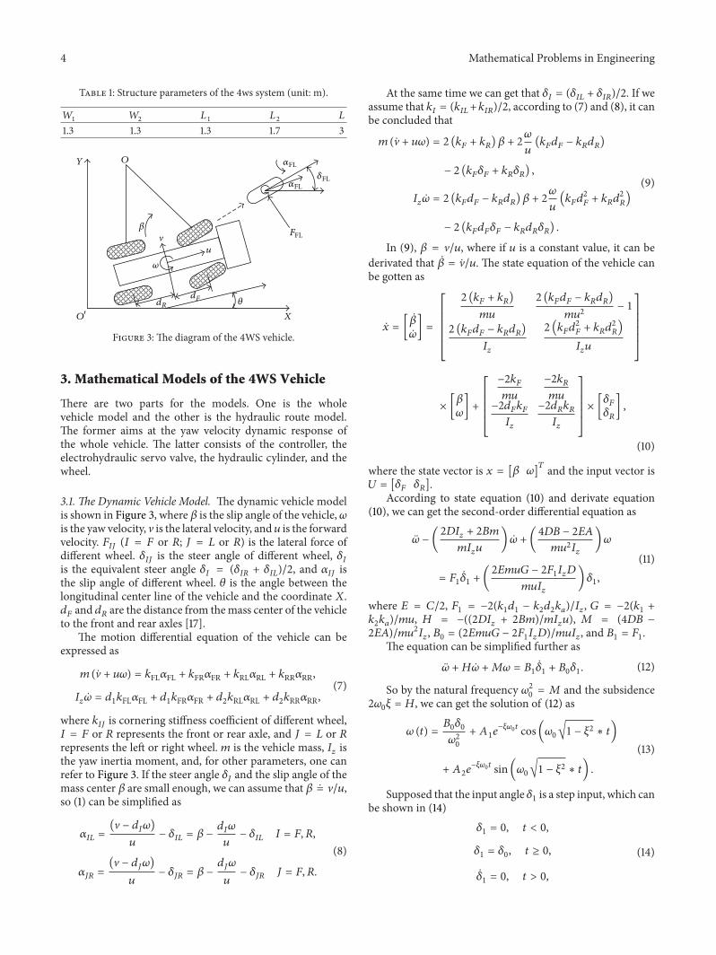
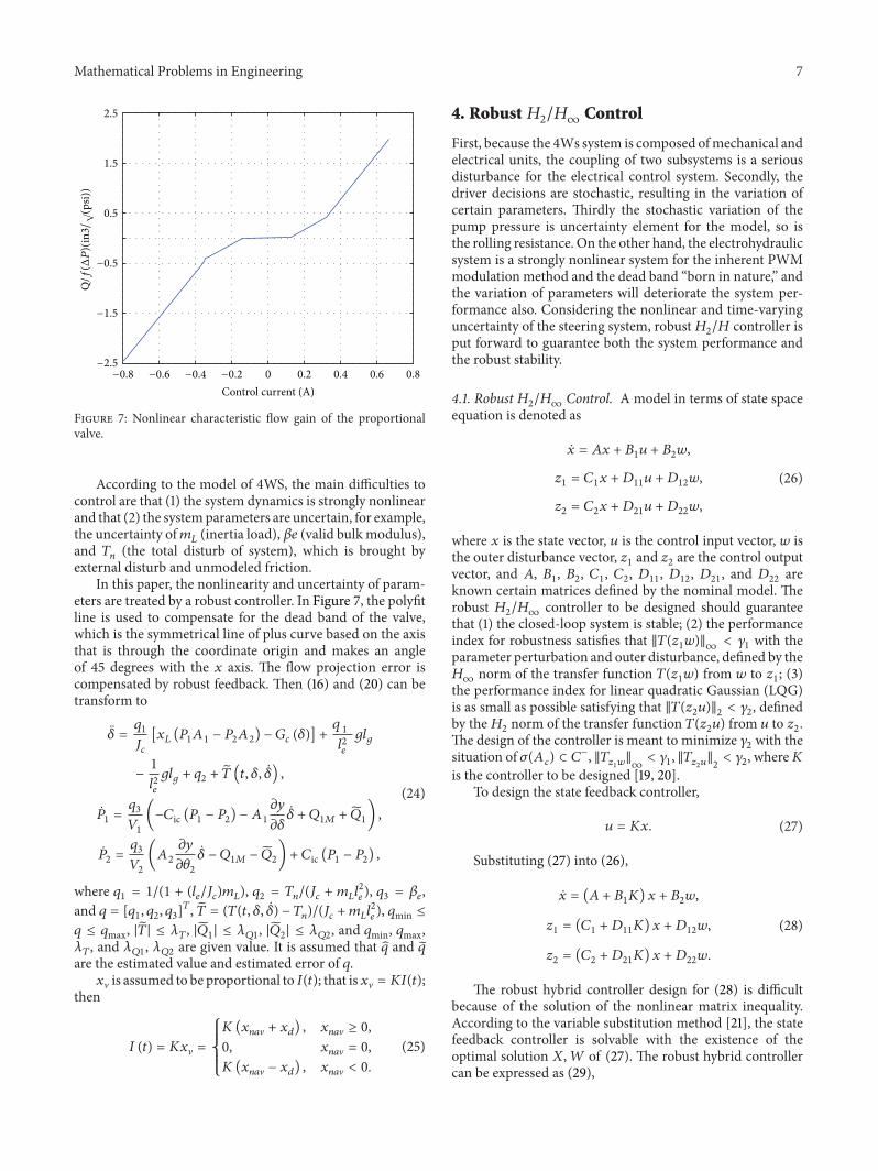
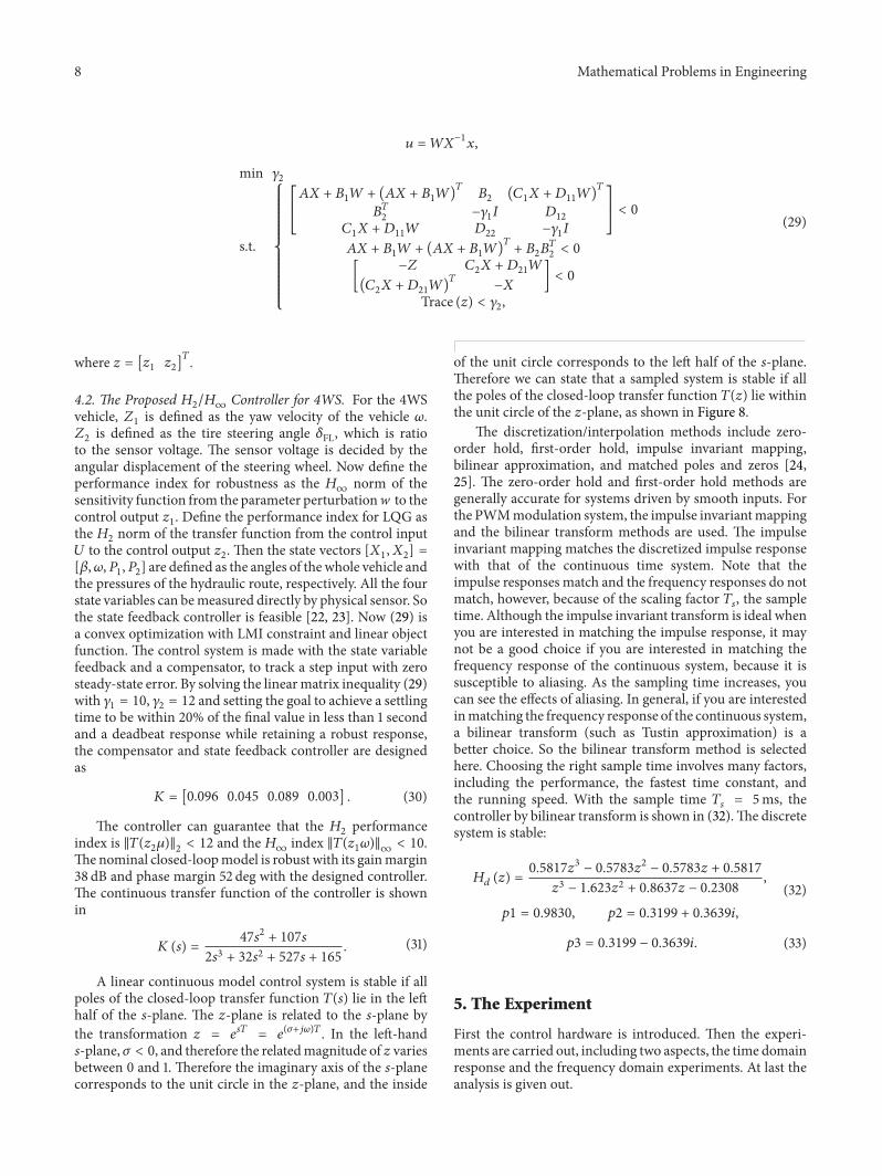
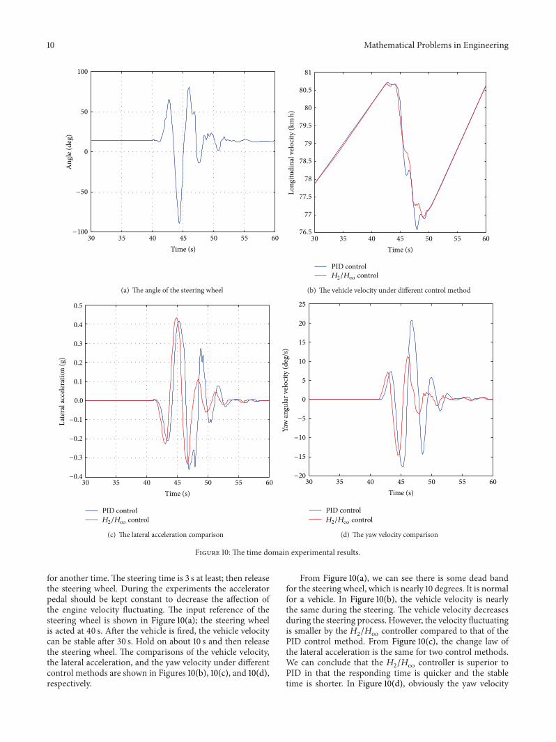
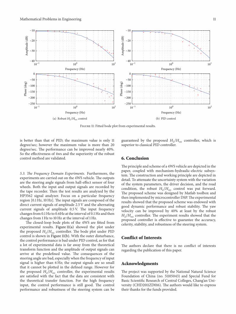