Control-Flow Analysis of Higher-Order Languages or Taming ... · Control-Flow Analysis of...
200
Control-Flow Analysis of Higher-Order Languages or Taming Lambda Olin Shivers May 1991 CMU-CS-91-145 School of Computer Science Carnegie Mellon University Pittsburgh, PA 15213 Submitted in partial fulfillment of the requirements for the degree of Doctor of Philosophy. c 1991 Olin Shivers This research was sponsored by the Office of Naval Research under Contract N00014-84-K-0415. The views and conclusions contained in this document are those of the author and should not be interpreted as representing the official policies, either expressed or implied, of ONR or the U.S. Government.
Transcript of Control-Flow Analysis of Higher-Order Languages or Taming ... · Control-Flow Analysis of...

Control-Flow Analysis of Higher-Order Languagesor
Taming Lambda
Olin Shivers
May 1991CMU-CS-91-145
School of Computer ScienceCarnegie Mellon University
Pittsburgh, PA 15213
Submitted in partial fulfillment of the requirementsfor the degree of Doctor of Philosophy.
c 1991 Olin Shivers
This research was sponsored by the Office of Naval Research under Contract N00014-84-K-0415. Theviews and conclusions contained in this document are those of the author and should not be interpreted asrepresenting the official policies, either expressed or implied, of ONR or the U.S. Government.

Keywords: data-flow analysis, Scheme, LISP, ML, CPS, type recovery, higher-orderfunctions, functional programming, optimising compilers, denotational semantics, non-standard abstract semantic interpretations

Abstract
Programs written in powerful, higher-order languages like Scheme, ML, and Common Lispshould run as fast as their FORTRAN and C counterparts. They should, but they don’t.A major reason is the level of optimisation applied to these two classes of languages.Many FORTRAN and C compilers employ an arsenal of sophisticated global optimisationsthat depend upon data-flow analysis: common-subexpression elimination, loop-invariantdetection, induction-variable elimination, and many, many more. Compilers for higher-order languages do not provide these optimisations. Without them, Scheme, LISP andML compilers are doomed to produce code that runs slower than their FORTRAN and Ccounterparts.The problem is the lack of an explicit control-flow graph at compile time, something whichtraditional data-flow analysis techniques require. In this dissertation, I present a techniquefor recovering the control-flow graph of a Scheme program at compile time. I give examplesof how this information can be used to perform several data-flow analysis optimisations,including copy propagation, induction-variable elimination, useless-variable elimination,and type recovery.The analysis is defined in terms of a non-standard semantic interpretation. The denotationalsemantics is carefully developed, and several theorems establishing the correctness of thesemantics and the implementing algorithms are proven.
iii

iv

To my parents, Julia and Olin.
v

vi
Contents
Acknowledgments xi
1 Introduction 1
1.1 My Thesis : : : : : : : : : : : : : : : : : : : : : : : : : : : : : : : : : 1
1.2 Structure of the Dissertation : : : : : : : : : : : : : : : : : : : : : : : : 2
1.3 Flow Analysis and Higher-Order Languages : : : : : : : : : : : : : : : : 3
2 Basic Techniques: CPS and NSAS 7
2.1 CPS : : : : : : : : : : : : : : : : : : : : : : : : : : : : : : : : : : : : 7
2.2 Control Flow in CPS : : : : : : : : : : : : : : : : : : : : : : : : : : : : 11
2.3 Non-Standard Abstract Semantic Interpretation : : : : : : : : : : : : : : 12
3 Control Flow I: Informal Semantics 15
3.1 Notation : : : : : : : : : : : : : : : : : : : : : : : : : : : : : : : : : : 15
3.2 Syntax : : : : : : : : : : : : : : : : : : : : : : : : : : : : : : : : : : : 16
3.3 Standard Semantics : : : : : : : : : : : : : : : : : : : : : : : : : : : : 17
3.4 Exact Control-Flow Semantics : : : : : : : : : : : : : : : : : : : : : : : 23
3.5 Abstract Control-Flow Semantics : : : : : : : : : : : : : : : : : : : : : 26
3.6 0CFA : : : : : : : : : : : : : : : : : : : : : : : : : : : : : : : : : : : : 31
3.7 Other Abstractions : : : : : : : : : : : : : : : : : : : : : : : : : : : : : 33
3.8 Semantic Extensions : : : : : : : : : : : : : : : : : : : : : : : : : : : : 34
4 Control Flow II: Detailed Semantics 41
4.1 Patching the Equations : : : : : : : : : : : : : : : : : : : : : : : : : : : 42
4.2 Abstraction Functions : : : : : : : : : : : : : : : : : : : : : : : : : : : 53
4.3 Existence : : : : : : : : : : : : : : : : : : : : : : : : : : : : : : : : : : 57
4.4 Properties of the Semantic Functions : : : : : : : : : : : : : : : : : : : 61
vii

5 Implementation I 79
5.1 The Basic Algorithm : : : : : : : : : : : : : : : : : : : : : : : : : : : : 79
5.2 Exploiting Monotonicity : : : : : : : : : : : : : : : : : : : : : : : : : : 80
5.3 Time-Stamp Approximations : : : : : : : : : : : : : : : : : : : : : : : 81
5.4 Particulars of My Implementation : : : : : : : : : : : : : : : : : : : : : 84
6 Implementation II 85
6.1 Preliminaries : : : : : : : : : : : : : : : : : : : : : : : : : : : : : : : : 85
6.2 The Basic Algorithm : : : : : : : : : : : : : : : : : : : : : : : : : : : : 86
6.3 The Aggressive-Cutoff Algorithm : : : : : : : : : : : : : : : : : : : : : 87
6.4 The Time-Stamp Algorithm : : : : : : : : : : : : : : : : : : : : : : : : 90
7 Applications I 93
7.1 Induction-Variable Elimination : : : : : : : : : : : : : : : : : : : : : : 93
7.2 Useless-Variable Elimination : : : : : : : : : : : : : : : : : : : : : : : 98
7.3 Constant Propagation : : : : : : : : : : : : : : : : : : : : : : : : : : : 101
8 The Environment Problem and Reflow Analysis 103
8.1 Limits of Simple Control-Flow Analysis : : : : : : : : : : : : : : : : : : 103
8.2 Reflow Analysis and Temporal Distinctions : : : : : : : : : : : : : : : : 105
9 Applications II: Type Recovery 107
9.1 Type Recovery : : : : : : : : : : : : : : : : : : : : : : : : : : : : : : : 107
9.2 Quantity-based Analysis : : : : : : : : : : : : : : : : : : : : : : : : : : 112
9.3 Exact Type Recovery : : : : : : : : : : : : : : : : : : : : : : : : : : : 112
9.4 Approximate Type Recovery : : : : : : : : : : : : : : : : : : : : : : : : 119
9.5 Implementation : : : : : : : : : : : : : : : : : : : : : : : : : : : : : : 127
9.6 Discussion and Speculation : : : : : : : : : : : : : : : : : : : : : : : : 128
9.7 Related Work : : : : : : : : : : : : : : : : : : : : : : : : : : : : : : : 133
10 Applications III: Super-� 135
10.1 Copy Propagation : : : : : : : : : : : : : : : : : : : : : : : : : : : : : 135
10.2 Lambda Propagation : : : : : : : : : : : : : : : : : : : : : : : : : : : : 137
10.3 Cleaning Up : : : : : : : : : : : : : : : : : : : : : : : : : : : : : : : : 141
10.4 A Unified View : : : : : : : : : : : : : : : : : : : : : : : : : : : : : : 141
viii

11 Future Work 14311.1 Theory : : : : : : : : : : : : : : : : : : : : : : : : : : : : : : : : : : : 14311.2 Other Optimisations : : : : : : : : : : : : : : : : : : : : : : : : : : : : 14411.3 Extensions : : : : : : : : : : : : : : : : : : : : : : : : : : : : : : : : : 14611.4 Implementation : : : : : : : : : : : : : : : : : : : : : : : : : : : : : : 149
12 Related Work 15112.1 Early Abstract Interpretation: the Cousots and Mycroft : : : : : : : : : : 15112.2 Hudak : : : : : : : : : : : : : : : : : : : : : : : : : : : : : : : : : : : 15212.3 Higher-Order Analyses: Deutsch and Harrison : : : : : : : : : : : : : : 153
13 Conclusions 155
Appendices
A 1CFA Code Listing 157A.1 Preliminaries : : : : : : : : : : : : : : : : : : : : : : : : : : : : : : : : 157A.2 1cfa.t : : : : : : : : : : : : : : : : : : : : : : : : : : : : : : : : : : : 161
B Analysis Examples 173B.1 Puzzle example : : : : : : : : : : : : : : : : : : : : : : : : : : : : : : 173B.2 Factorial example : : : : : : : : : : : : : : : : : : : : : : : : : : : : : 176
Bibliography 179
ix

x

Acknowledgments
It is a great pleasure to thank the people who helped me with my graduate career.
First, I thank the members of my thesis committee: Peter Lee, Allen Newell, JohnReynolds, Jeannette Wing, and Paul Hudak.
� Peter Lee, my thesis advisor and good friend, taught me how to do research, taughtme how to write, helped me publish papers, and kept me up-to-date on the latestdevelopments in Formula-1 Grand Prix. I suppose that I recursively owe a debt toUwe Pleban for teaching Peter all the things he taught me.
� Allen Newell was my research advisor for my first four years at CMU, and co-advisedme with Peter after I picked up my thesis topic. He taught me about having “a brightblue flame for science.” Allen sheltered me during the period when I was drifting inresearch limbo; I’m reasonably certain that had I chosen a different advisor, I’d havebecome an ex-Ph.D.-candidate pretty rapidly. Allen believed in me — certainly morethan I did.
� John Reynolds taught (drilled/hammered/beat into) me the importance of formalrigour in my work. Doing mathematics with John is an exhilarating experience, ifyou have lots of stamina and don’t mind chalk dust or feelings of inadequacy. John’semphasis on formal methods rescued my dissertation from being just another pile ofhacks.
� Jeannette Wing was my contact with the programming-systems world while I wasofficially an AI student. She supported my control-flow analysis research in its earlystages. She also has an eagle eye for poor writing and a deep appreciation for edgedweapons.
� Paul Hudak’s work influenced me a great deal. His papers on abstract semanticinterpretations caused me to consider applying the whole approach to my problem.
It goes without saying that all of these five scholars are dedicated researchers, else theywould not have attained their current positions. However—and this is not a given inacademe—they also have a deep committment to their students’ welfare and development.I was very, very lucky to be trained in the craft of science under the tutelage of theseindividuals.
xi
In the summer of 1984, Forest Baskett hired the entire T group to come to DEC’sWestern Research Laboratory and write a Scheme compiler. I was going to do the data-flowanalysis module of the compiler; it would be fair to say that I am now finally finishing my1984 summer job. The compiler Forest hired us to write turned into the ORBIT Schemecompiler, and this dissertation is the third one to come out of that summer project (sofar). Both Forest and DEC have a record of sponsoring grad students for summer researchprojects that are interesting longshots, and I’d like to acknowledge their foresight, scopeand generosity.
If one is going to do research on advanced programming languages, it certainly helps tobe friends with someone like Jonathan Rees. In 1982, Jonathan was the other guy at Yalewho’d read the Sussman/Steele papers. We agreed that hacking Scheme and spinning greatplans was much more fun than interminable theory classes. Jonathan’s deep understandingof computer languages and good systems taste has influenced me repeatedly.
Norman Adams, like Jonathan a member of the T project, contributed his technical andmoral support to my cause. The day you need your complex, forty-page semantics paperreviewed and proofread in forty-eight hours is the day you really think hard about who yourfriends are.
David Dill has an amazing ability. He will listen to you describe a problem he’s neverthought about before. Then, after about twenty minutes, he will make a two-sentenceobservation; it will cut right to the heart of your problem. (Stanford grad students lookingfor an advisor should note this fact carefully.) David patiently listened to me ramble onabout doing data-flow analysis in Scheme long before I had the confidence to discuss itwith anyone else. Our discussions helped me to overcome early discouragement and hissuggestions led, as they usually do, straight toward the eventual solution.
CMU Computer Science is well known for its cooperative, friendly environment. WhenI was deep into the formal construction of the analyses in some precursor work to this dis-sertation, I got completely hung up on a tricky, non-standard recursive domain construction.The prospect of having to do my very own inverse-limit construction was not a thrillingone. One Saturday morning, the phone rang about three hours after I had gone to sleep.It was Dana Scott, who proceeded to read to me over the phone a four-line solution to myproblem. John Reynolds had described my problem to him in the hall on Friday; Dana hadtaken it home and solved it. This episode is typical of the close support and cooperationthat has made my time here as a graduate student so pleasant and intellectually fulfilling.
Alan Perlis, Josh Fisher, and John Ellis were instrumental in teaching me the art ofprogramming at Yale and persuaded me by example that getting a Ph.D. in computerscience was obviously the most interesting and fun thing one could possibly do aftercollege. Mary-Claire van Leunen, also at Yale, did what she could to improve my writingstyle. Professors Ferdinand Levy and Hyland Chen were also, by way of example, largeinfluences on my decision to pursue a research degree. Perlis and Levy, in particular, soldme on the idea of coming to CMU.
The core of my knowledge of denotational semantics comes from a grad student classgiven by Stephen Brookes. His lecture notes, which he is currently converting into a book,
xii

were a clear and painless introduction to the field. When I began work on the formalsemantics part of this dissertation, I repeatedly returned to them.
Heather, Lin, Olga, and Wenling provided emotional first-aid and kept me glued togetherduring black times. Mark Shirley, my hacking partner and good friend, gets credit forhanding me a set of Sussman and Steele’s papers in 1980, which, it could be argued,triggered off the next decade of my life. Had Manuel Hernandez and Holt Sanders notbeen with me on the deck of the Jing Lian Hao during a typhoon in the South China Sea inthe summer of 1986, I would not have had a next decade of my life, and this dissertation,obviously, would never have been written. Small decisions. . .
Having the office one down from Hans Moravec’s for five years is bound to warpanybody, particularly if you share the same circadian cycle.1 Late-night exposure toHans, a genuine Mad Scientist, taught me about relativistic Star Wars, skyhooks, neuraldevelopment in chordates, life in the sun, methods for destroying the universe, robotpals, the therapeutic value of electrical shock, material properties of magnetic monopoles,downloading your software, and the tyranny of the 24-hour cycle. Generally speaking,Hans kept my mind loosened up.
It must be said that my officemates, Rich Wallace, Hans Tallis, Derek Beatty, AllanHeydon, and Hank Wan, are very patient people. Particularly with respect to phone bills.
Finally, of course, I want to thank my family, particularly my parents, Julia and Olin;my sisters, Julia and Mary; and my uncle, Laurence. It has helped a great deal knowingthat their unstinting love and support was always there.
1I.e., the rotational period of Mars.
xiii

xiv
Chapter 1
Introduction
1.1 My Thesis
Control-flow analysis is feasible and useful for higher-order languages.
Higher-order programming languages, such as Scheme and ML, are more difficult toimplement efficiently than more traditional languages such as C or FORTRAN. Complex,state-of-the-art Scheme compilers can produce code that is roughly as efficient as thatproduced by simple, non-optimising C compilers [Kranz+ 86]. However, Scheme and MLcompilers still cannot compete successfully with complex, state-of-the-art C and FORTRAN
compilers.
A major reason for this gap is the level of optimisation applied to these two classesof languages. Many FORTRAN and C compilers employ an arsenal of sophisticated globaloptimisations that depend upon data-flow analysis: common-subexpression elimination,loop-invariant detection, induction-variable elimination, and many, many more. Schemeand ML compilers do not provide these optimisations. Without them, these compilers aredoomed to produce code that runs slower than their FORTRAN and C counterparts.
One key problem is the lack of an explicit control-flow graph at compile time, somethingtraditional data-flow analysis techniques require. In this dissertation, I develop an analysisfor recovering the control-flowgraph from a Scheme program at compile time. This analysisuses an intermediate representation called CPS, or continuation-passing style, and a generalanalysis framework called non-standard abstract semantic interpretation.
After developing the analysis, I present proofs of its correctness, give algorithms forcomputing it, and discuss implementation tricks that can be applied to the algorithms. Thisestablishes the first half of my thesis: control-flow analysis is feasible for higher-orderlanguages.
The whole point of control-flow analysis is that it enables important data-flow programoptimisations. To demonstrate this, I use the results of the control-flow analysis to developseveral of these classical data-flow analyses and optimisations for higher-order languages.This establishes the second half of my thesis: control-flow analysis is useful for higher-orderlanguages.
1

2 Chapter 1. Introduction
1.2 Structure of the Dissertation
This dissertation has the following structure:
� The rest of this chapter discusses data-flow analysis, higher-order languages, and whyit is difficult to do the one in the other.
� The following chapter (2) introduces the two basic tools we’ll need to develop theanalysis: the CPS intermediate representation, and the technique of non-standardabstract semantic interpretation.
� Next we develop the basic control-flow analysis. Chapter 3 presents the analysis; thisis the core of the dissertation. Chapter 4 contains proofs that establish the analysis’correctness and computability.
� After developing the analysis as a mathematical function, we turn to algorithms forcomputing this function. Chapter 5 develops the algorithms, and discusses somedetails of an implementation that I wrote. Chapter 6 contains proofs showing that thealgorithms compute the analysis function.
� Chapter 7 develops three applications using control-flow analysis: induction-variableelimination, useless-variable elimination, and constant propagation.
� Control-flow analysis has limitations. Chapter 8 discusses these limits, and presentsan extension (reflow analysis) that can be used to exceed them. Chapters 9 and 10discuss four more applications that rely on reflow analysis: type recovery, futureanalysis, copy propagation, and lambda propagation.
� The dissertation proper closes with chapters on future directions, related work, andconclusions (chapters 11–13).
� This is followed by two appendices, one containing a code listing for a control-flowanalysis implementation, and one giving the results of applying this program to somesimple Scheme procedures.
1.2.1 Skipping the Math
This dissertation has a fair amount of mathematics in it, mostly denotational semantics. Inspite of this, I have made a particular effort to make it comprehensible to the reader whoprefers writing programs to proving theorems. Most of the serious mathematics is carefullysegregated into distinct chapters; each of these chapters begins with a half-page summarythat states the chapter’s main results. Feel free to read the summary, take the results onfaith, and skip the math.

1.3. Flow Analysis and Higher-Order Languages 3
1.3 Flow Analysis and Higher-Order Languages
1.3.1 Flow Analysis
Flow analysis is a traditional optimising compiler technique for determining useful infor-mation about a program at compile time. Flow analysis determines path-invariant factsabout textual points in a program. A flow analysis problem is a question of the form:
“What is true at a given textual point p in my program, independent of theexecution path taken to p from the start of the program?”
Example domains of interest might be the following:
� Range analysis: What range of values is a given reference to an integer variableconstrained to lie within? Range analysis can be used, for instance, to do arraybounds checking at compile time.
� Loop invariant detection: Do all possible prior assignments to a given variablereference lie outside its containing loop?
Over the last thirty years, standard techniques have been developed [Aho+ 86, Hecht 77]to answer these questions for the standard imperative languages (e.g., Pascal, C, Ada, Bliss,and chiefly FORTRAN). Flow analysis is perhaps the chief tool in the optimising compilerwriter’s bag of tricks; figure 1.1 gives a partial list of the code optimisations that can beperformed using flow analysis.
1.3.2 Higher-Order Languages
A higher-order programming language (HOL) is one that permits higher-order procedures— procedures that can take other procedures as arguments and return them as results. Morespecifically, I am interested in the class of lexically scoped, applicative order languagesthat allow side-effects and provide procedures as first-class data. Members of this class areScheme [Rees+ 86], ML [Milner 85, Milner+ 90], and Common Lisp [Steele 90]. Granting“first class” status to procedures means allowing them to be manipulated with the samefreedom as other primitive data types, e.g., passing them as arguments to procedures,returning them as values, and storing them into data structures.
In this dissertation, I shall use Scheme as the exemplar of higher-order languages, andonly occasionally refer to other languages. Scheme is a small, simple language, whichnonetheless has the full set of features that conspire to make flow analysis so difficult:higher-order procedures, side effects, and compound data structures. ML’s principal se-mantic distinction from Scheme, its type system, does not fundamentally affect the task offlow analysis. The size and complexity of Common Lisp make it difficult to work with,but do not introduce any interesting new semantic features that change the flow analysisproblem.
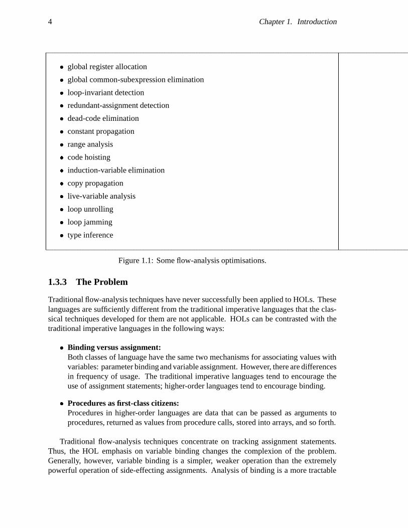
4 Chapter 1. Introduction
� global register allocation
� global common-subexpression elimination
� loop-invariant detection
� redundant-assignment detection
� dead-code elimination
� constant propagation
� range analysis
� code hoisting
� induction-variable elimination
� copy propagation
� live-variable analysis
� loop unrolling
� loop jamming
� type inference
Figure 1.1: Some flow-analysis optimisations.
1.3.3 The Problem
Traditional flow-analysis techniques have never successfully been applied to HOLs. Theselanguages are sufficiently different from the traditional imperative languages that the clas-sical techniques developed for them are not applicable. HOLs can be contrasted with thetraditional imperative languages in the following ways:
� Binding versus assignment:Both classes of language have the same two mechanisms for associating values withvariables: parameter binding and variable assignment. However, there are differencesin frequency of usage. The traditional imperative languages tend to encourage theuse of assignment statements; higher-order languages tend to encourage binding.
� Procedures as first-class citizens:Procedures in higher-order languages are data that can be passed as arguments toprocedures, returned as values from procedure calls, stored into arrays, and so forth.
Traditional flow-analysis techniques concentrate on tracking assignment statements.Thus, the HOL emphasis on variable binding changes the complexion of the problem.Generally, however, variable binding is a simpler, weaker operation than the extremelypowerful operation of side-effecting assignments. Analysis of binding is a more tractable

1.3. Flow Analysis and Higher-Order Languages 5
problem than analysis of assignments because the semantics of binding are simpler andthere are more invariants for program-analysis tools to invoke. In particular, the invariantsof the �-calculus are usually applicable to HOLs.
On the other hand, the higher-order, first-class nature of HOL procedures can hinderefforts to derive even basic control-flow information. I claim that it is this aspect of higher-order languages which is chiefly responsible for the absence of flow analysis from theircompilers to date. A brief discussion of traditional flow analysis techniques will show whythis is so.
Consider the following piece of Pascal code:
FOR i := 0 to 30 DO BEGIN
s := a[i];
IF s < 0 THEN
a[i] := (s+4)^2
ELSE
a[i] := cos(s+4);
b[i] := s+4;
END
Traditional flow analysis requires construction of a control-flow graph for the code fragment(fig. 1.2).
�
�START
i:=0
i<=30?
s:=a[i]
s<0?
a[i]:=(s+4)^2
b[i]:=s+4
i:=i+1
�
�STOP
a[i]:=cos(s+4)?
-
?
?
?
-
�
-
-
Figure 1.2: Control-flow graph
Every vertex in the graph represents a basic block of code: a sequence of instructionssuch that the only branches into the block are branches to the beginning of the block, and theonly branches from the block occur at the end of the block. The edges in the graph representpossible transfers of control between basic blocks. Having constructed the control-flowgraph, we can use graph algorithms to determine path invariant facts about the vertices.
In this example, for instance, we can determine that on all control paths from START tothe dashed block (b[i]:=s+4;i:=i+1), the expression s+4 is evaluated with no subsequentassignments to s. Hence, by caching the result of s+4 in a temporary, we can eliminate theredundant addition in b[i]:=s+4. We obtain this information through consideration of thepaths through the control-flow graph.

6 Chapter 1. Introduction
The problem with HOLs is that there is no static control-flow graph at compile time.Consider the following fragment of Scheme code:
(let ((f (foo 7 g k))
(h (aref a7 i j)))
(if (< i j) (h 30) (f h)))
Consider the control flow of the if expression. Its graph is: i<j?
f
h
?
-
After evaluating the conditional’s predicate, control can transfer either to the procedure thatis the value of h, or to the procedure that is the value of f. But what’s the value of f?What’s the value of h? Unhappily, they are computed at run time.
If we knew all the procedures that h and f could possibly be bound to, independentof program execution, we could build a control-flow graph for the code fragment. So, ifwe wish to have a control-flow graph for a piece of Scheme code, we need to answer thefollowing question: for every procedure call in the program, what are the possible lambdaexpressions that call could be a jump to? But this is a flow analysis question! So withregard to flow analysis in an HOL, we are faced with the following unfortunate situation:
� In order to do flow analysis, we need a control-flow graph.
� In order to determine control-flow graphs, we need to do flow analysis.

Chapter 2
Basic Techniques: CPS and NSAS
2.1 CPS
The fox knows many things, but the hedgehogknows one great thing.
— Archilocus
The first step towards finding a solution to this conundrum is to develop a representationfor our programs suitably adapted to the analysis we’re trying to perform.
In Scheme and ML, we must represent and deal with transfers of control caused byprocedure calls. In the interests of simplicity, then, we adopt a representation where alltransfers of control — sequencing, looping, procedure call/return, conditional branching —are represented with the same mechanism: the tail-recursive procedure call. This type ofrepresentation is called Continuation-Passing Style or CPS.
Our intermediate representation, CPS Scheme, stands in contrast to the intermediaterepresentation languages commonly chosen for traditional optimising compilers. Theselanguages are conventionally some form of slightly cleaned-up assembly language: quads,three-address code, or triples. The disadvantage of such representations is their ad hoc,machine-specific, and low-level semantics. The advantages of CPS Scheme lie in its appealto the formal semantics of the �-calculus and its representational simplicity.
CPS conversion can be referred to as the “hedgehog” approach, after a quotation byArchilocus. All control and environment structures are represented in CPS by lambdaexpressions and their application. After CPS conversion, the compiler need only know“one great thing” — how to compile lambda expressions very well. This approach has aninteresting effect on the pragmatics of Scheme compilers. Basing the compiler on lambdaexpressions makes lambda expressions very cheap, and encourages the programmer to usethem explicitly in his code. Since lambda is a very powerful construct, this is a considerableboon for the programmer.
7
8 Chapter 2. Basic Techniques: CPS and NSAS
2.1.1 Definition of CPS Scheme
CPS can be summarised by stating that procedure calls in CPS are one-way transfers —they do not return. So a procedure call can be viewed as a GOTO that passes values. Ifwe are interested in the value computed by a procedure f of two values, we must alsopass to f a third argument, the continuation. The continuation is a procedure; after fcomputes its value v, instead of “returning” the value v, it calls the continuation on v.Thus the continuation represents the control point to which control should transfer after theexecution of f .
For example, if we wish to print the value computed by (x+ y) � (z � w), we do notwrite:
(print (* (+ x y) (- z w)))
Instead, we write:
(+ x y (� (xy)
(- z w (� (zw)
(* xy zw (� (prod) (print prod *c*)))))))
Here, the original procedures — +, -, *, and print— are all redefined to take a continuationas an extra argument. The + procedure calls its third argument, (� (xy) . . . ), on the sumof its first two arguments, x and y. Likewise, the - procedure calls its third argument,(� (zw) . . .), on the difference of its first two arguments, z and w. The * procedure callsits third argument on the product of its first two arguments, x+ y and z �w. This productis finally passed to the print procedure, along with some top-level continuation *c*. Theprint procedure prints out the value of prod and then calls the *c* continuation.
Standard non-CPS Scheme can be easily transformed into an equivalent CPS program,so this representation carries no loss of generality. Once committed to CPS, we can makefurther simplifications:
� No special syntactic forms for conditional branchThe semantics of primitive conditional branch is captured by the primitive procedureifwhich takes one boolean argument, and two continuation arguments: (if b c a).If the boolean b is true, the true, or “consequent,” continuation c is called; otherwise,the false, or “alternate,” continuation a is called.
We can also assume a class of test primitives that perform various basic conditionaltests on their first argument. For example, (test-integer x c a) branches tocontinuation c if x is an integer, otherwise to continuation a.
� No side effects to variablesSide effects are allowed to data structures only. That is, the programmer is allowed toalter the contents of data structures, with operations like rplaca and vector-set!,but he is not allowed to alter the bindings of variables — there is no set! syntax. Thismeans that all side-effects are handled by primitive operations, and special syntax isnot required.

2.1. CPS 9
� Lambda expressions: (� (v1 . . . vn) call)where n � 0.
� Variable references: foo, bar, . . .
� Constants: 3, "doghen", '(a 3 elt list), . . .
� Primitive operations: +, if, rplaca, . . .
� Simple calls: ( fun arg� )
where fun is a lambda, var, or primop, and the args are lambdas, vars, or constants.
� letrec calls: (letrec ((f1 l1). . . ) call)where the fi are variables, and the li are lambda expressions.
Figure 2.1: CPS Scheme language grammar
Programs that use variable assignment can be automatically converted to assignment-free programs by inserting extra mutable data structures into the program. Anexpression that looks like
(� (x) . . . (set! x y) . . . x . . . )
is converted to
(� (x')
(let ((x (make-cell x')))
. . . (set-cell x y) . . . (contents x) . . . ))
This process is called “assignment conversion” [Kranz+ 86].
� No call/cc operatorLanguages like Scheme and ML often have the troublesome call-with-current-continuation or call/cc operator. CPS Scheme doesn’t need the operator. Whentranslating programs into their CPS Scheme representations, every occurrence ofcall/cc can be replaced with its CPS definition:
(� (f k) (f (� (v k0) (k v)) k))
Scheme code violating any of these restrictions is easily mapped into equivalent Schemecode preserving them, so they also carry no loss of generality. The details of the CPS trans-formation are treated in a number of papers [Kelsey 89, Kranz 88, Kranz+ 86, Steele 76].These restrictions leave us with a fairly simple language to deal with: There are only fivesyntactic classes: lambdas, variables, constants, primitive operations (or primops) and calls(fig. 2.1). Note that primops are not first-class citizens — in this grammar, they may onlybe called, not used as arguments, or passed around as data. This is not a problem, since
10 Chapter 2. Basic Techniques: CPS and NSAS
(� (n) (letrec ((lp (� (i sum) (if (zero? i) sum
(lp (- i 1) (+ i sum))))))
(lp n 0)))
(� (n k)
(letrec ((lp (� (i sum c)
(test-zero i
(� () (c sum))
(� ()
(- i 1 (� (i1)
(+ sum i (� (sum1)
(lp i1 sum1 c))))))))))
(lp n 0 k)))
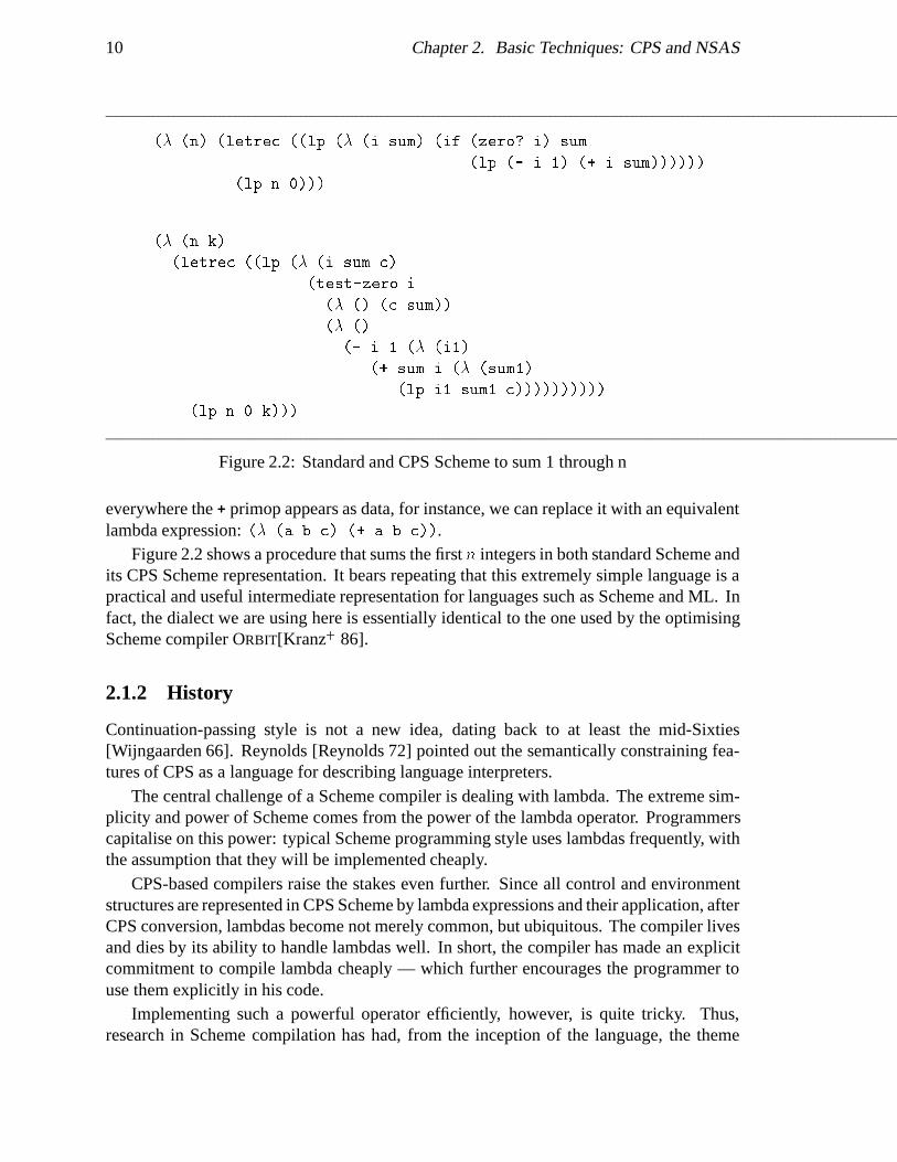
Figure 2.2: Standard and CPS Scheme to sum 1 through n
everywhere the + primop appears as data, for instance, we can replace it with an equivalentlambda expression: (� (a b c) (+ a b c)).
Figure 2.2 shows a procedure that sums the first n integers in both standard Scheme andits CPS Scheme representation. It bears repeating that this extremely simple language is apractical and useful intermediate representation for languages such as Scheme and ML. Infact, the dialect we are using here is essentially identical to the one used by the optimisingScheme compiler ORBIT[Kranz+ 86].
2.1.2 History
Continuation-passing style is not a new idea, dating back to at least the mid-Sixties[Wijngaarden 66]. Reynolds [Reynolds 72] pointed out the semantically constraining fea-tures of CPS as a language for describing language interpreters.
The central challenge of a Scheme compiler is dealing with lambda. The extreme sim-plicity and power of Scheme comes from the power of the lambda operator. Programmerscapitalise on this power: typical Scheme programming style uses lambdas frequently, withthe assumption that they will be implemented cheaply.
CPS-based compilers raise the stakes even further. Since all control and environmentstructures are represented in CPS Scheme by lambda expressions and their application, afterCPS conversion, lambdas become not merely common, but ubiquitous. The compiler livesand dies by its ability to handle lambdas well. In short, the compiler has made an explicitcommitment to compile lambda cheaply — which further encourages the programmer touse them explicitly in his code.
Implementing such a powerful operator efficiently, however, is quite tricky. Thus,research in Scheme compilation has had, from the inception of the language, the theme

2.2. Control Flow in CPS 11
of taming lambda: using compile-time analysis techniques to recognise and optimise thelambda expressions that do not need the fully-general closure implementation.
This thesis extends a thread of research on CPS-based compilers that originates with thework of Steele and Sussman in the mid-seventies. CPS and its merits are treated at length bySteele and Sussman. Their 1976 paper, “Lambda: The Ultimate Declarative” [Steele 76],first introduced the possibility of using CPS as an intermediate representation for a Schemecompiler. Steele designed and implemented such a compiler, Rabbit, for his Master’s thesis[Steele 78]. Rabbit demonstrated that Scheme could be compiled efficiently, and showedthe effectiveness of CPS-based compiler technology. Rabbit introduced the idea of codeanalysis to aid the compiler in translating lambdas into efficient code.
The next major development in CPS-based compilation was the ORBIT Scheme compiler[Kranz+ 86], designed and implemented by the T group [Rees+ 82] at Yale. ORBIT wasa strong demonstration of the power of CPS-based compilers: it produced code that wascompetitive with non-optimising C and Pascal compilers. ORBIT, again, relied on extensiveanalysis of the CPS code tree to separate the “easy” lambdas, which could be compiled intoefficient code, from the lambdas that needed general but less-efficient run-time realisations.The most detailed explication of these analyses is found in Kranz’s dissertation [Kranz 88].ORBIT is the most highly optimising Scheme compiler extant.
Kelsey, also a member of the T group, has designed a compiler, TC, whose middle andback ends employ a CPS intermediate representation [Kelsey 89]. He has front ends whichtranslate BASIC, Scheme and Pascal into CPS.
A team at Princeton and Bell Labs, led by Andrew Appel and David MacQueen, hasapplied the Orbit technology to ML with good results [Appel+ 89]. Their CPS-basedcompiler is currently the standard compiler for most ML programming in the U.S.
CPS is now an accepted representation for advanced language compilers. None ofthese compilers, however, has made a significant attempt to perform control- or data-flowanalysis on the CPS form. This thesis, then, is an attempt to push CPS-based compilers tothe next stage of sophistication.
2.2 Control Flow in CPS
The point of using CPS Scheme for an intermediate representation is that all transfers ofcontrol are represented by procedure call. This gives us a uniform framework in which todefine the control-flow analysis problem. In the CPS Scheme framework, the control-flowproblem is defined as follows:
For each call site c in program P , find a set L(c) containing all the lambdaexpressions that could be called at c. I.e., if there is a possible execution of Psuch that lambda l is called at call site c, then l must be an element of L(c).
That is, control-flow analysis in CPS Scheme consists of determining what call sites callwhich lambdas.
12 Chapter 2. Basic Techniques: CPS and NSAS
This definition of the problem does not define a unique function L. The trivial solutionis the function L(c) = AllLambdas, i.e., the conclusion that all lambdas can be reachedfrom any call site. What we want is the tightest possible L that we can derive at compiletime with reasonable computational expense.
2.3 Non-Standard Abstract Semantic Interpretation
2.3.1 NSAS
Casting our problem into this CPS-based framework gives us a structure to work with; wenow need a technique for analysing that structure. The method of non-standard abstractsemantics (NSAS) is an elegant technique for formally describing program analyses. Itforms the tool we’ll use to solve our control-flow problem as described in the previoussection.
Suppose we have programs written in some programming language L, and we wish todetermine some property X about our programs at compile time. For example, X might bethe property “the set of variables in a program whose values may be stack-allocated insteadof heap-allocated.” There is a three-step process we can use in the NSAS framework toconstruct a computable analysis for X:
1. We start with a standard denotational semantics S for our language. This gives us aprecise definition of what the programs written in our language mean.
2. Then, we develop a non-standard semanticsSX forL that precisely expresses propertyX . We typically derive this non-standard semantics from our original standardsemantics S. So, whereas semantics S might say the meaning of a program is afunction mapping the program’s inputs to its results, semantics SX would say themeaning of a program is a function mapping the program’s inputs to the property X .The point of this semantics is that it constitutes a precise, formal definition of theproperty we want to analyse.
3. SX is a precise definition of the property we wish to determine, but its precision typ-ically implies that it cannot be computed at compile time. It might be uncomputable;it might also depend on the run-time inputs. The final step, then, is to abstract SXto a new semantics, bSX which trades accuracy for compile-time computability. Thissort of approximation is a typical program-analysis tradeoff — the real answers weseek are uncomputable, so we settle for computable, conservative approximations tothem.
When we are done, we have a computable analysis bSX , and two other semantics that linkit back to the real, standard semantics for our language.
The method of abstract semantic interpretation has several benefits. Since an NSAS-based analysis is expressed in terms of a formal semantics, it is possible to prove importantproperties about it. In particular, we can prove that the non-standard semantics SX correctly
2.3. Non-Standard Abstract Semantic Interpretation 13
expresses properties of the standard semantics S, and that the abstract semantics bSX iscomputable and safe with respect to SX . Further, due to its formal nature, and becauseof its relation to the standard semantics of a programming language, simply expressing ananalysis in terms of abstract semantic interpretations helps to clarify it.
NSAS-based analyses have been developed for an array of program optimisations.Typical examples are strictness analysis of normal-order languages [Bloss+ 86] and staticreclamation of dynamic data-structures (“compile-time gc”) [Hudak 86b].
2.3.2 Don’t Panic
The reader who is more comfortable with computer languages than denotational semanticsequations should not despair. The semantic equations presented in this dissertation canquite easily be regarded as interpreters in a functional disguise. The important point is thatthese “interpreters” do not compute a program’s actual value, but some other property ofthe program (in our case, the call graph for the program). We will compute this call graphwith a non-standard, abstract “interpreter” that abstractly executes the program, collectinginformation as it goes.
2.3.3 NSAS Example
The traditional toy example [Cousot 77, Mycroft 81] of an NSAS-based analysis uses thearithmetic rule of signs. The rule of signs is simply the property of arithmetic that tellsus the sign of simple arithmetic operations based on the sign of their operands: a positivenumber times a negative number is negative, a negative number minus a positive numberis negative, and so forth.
Consider a simple language that allows us to add, subtract, and multiply integer con-stants. A typical expression in our language might be
-3 * (3 + (-4 - 2))
Suppose we’re interested in determining the sign of an expression without having to actuallycompute its full value.
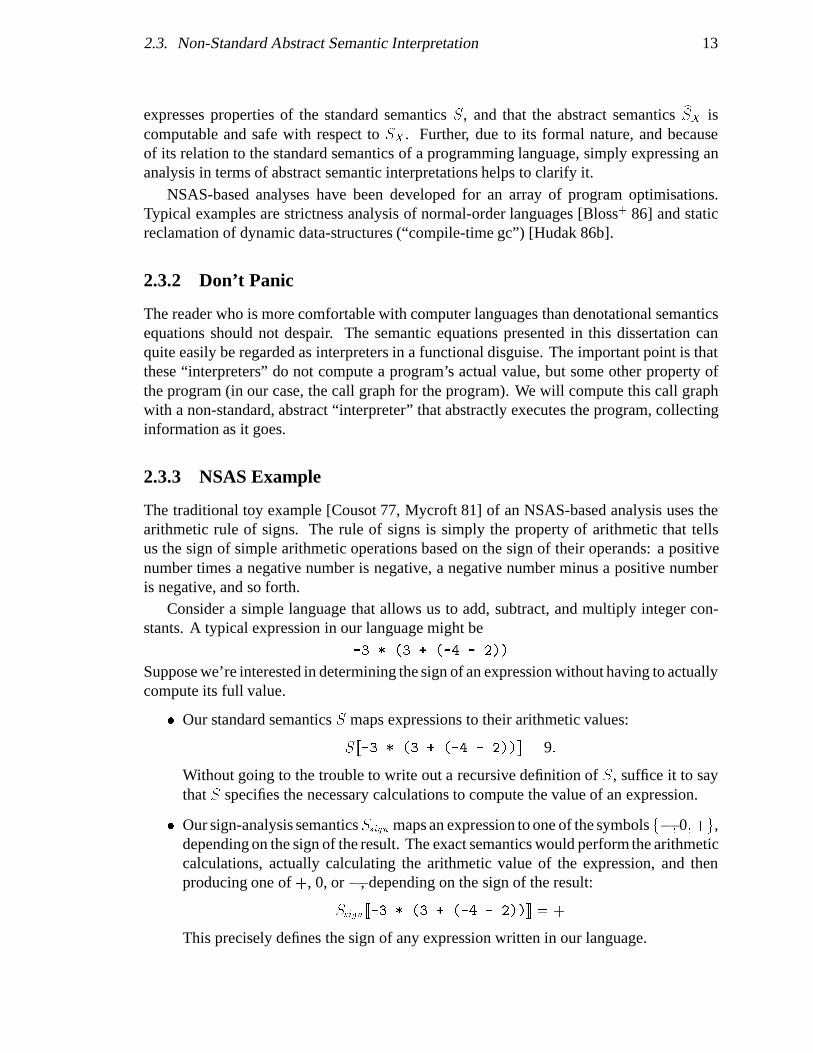
� Our standard semantics S maps expressions to their arithmetic values:
S[[-3 * (3 + (-4 - 2))]] = 9:
Without going to the trouble to write out a recursive definition of S, suffice it to saythat S specifies the necessary calculations to compute the value of an expression.
� Our sign-analysis semanticsSsign maps an expression to one of the symbolsf�; 0;+g,depending on the sign of the result. The exact semantics would perform the arithmeticcalculations, actually calculating the arithmetic value of the expression, and thenproducing one of +, 0, or �, depending on the sign of the result:
Ssign [[-3 * (3 + (-4 - 2))]] = +
This precisely defines the sign of any expression written in our language.
14 Chapter 2. Basic Techniques: CPS and NSAS
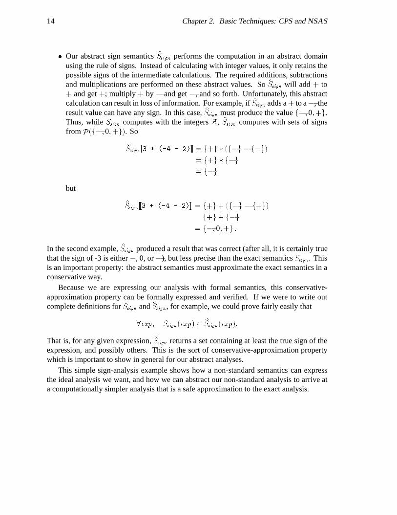
� Our abstract sign semantics bSsign performs the computation in an abstract domainusing the rule of signs. Instead of calculating with integer values, it only retains thepossible signs of the intermediate calculations. The required additions, subtractionsand multiplications are performed on these abstract values. So bSsign will add + to+ and get +; multiply + by � and get �, and so forth. Unfortunately, this abstractcalculation can result in loss of information. For example, if bSsign adds a + to a�, theresult value can have any sign. In this case, bSsign must produce the value f�; 0;+g.Thus, while Ssign computes with the integers Z , bSsign computes with sets of signsfrom P(f�;0;+g). So
bSsign [[3 * (-4 - 2)]] = f+g � (f�g � f+g)
= f+g � f�g
= f�g
but
bSsign [[3 + (-4 - 2)]] = f+g+ (f�g � f+g)
= f+g+ f�g
= f�;0;+g :
In the second example, bSsign produced a result that was correct (after all, it is certainly truethat the sign of -3 is either +, 0, or �), but less precise than the exact semantics Ssign . Thisis an important property: the abstract semantics must approximate the exact semantics in aconservative way.
Because we are expressing our analysis with formal semantics, this conservative-approximation property can be formally expressed and verified. If we were to write outcomplete definitions for Ssign and bSsign , for example, we could prove fairly easily that
8exp; Ssign(exp) 2 bSsign(exp):
That is, for any given expression, bSsign returns a set containing at least the true sign of theexpression, and possibly others. This is the sort of conservative-approximation propertywhich is important to show in general for our abstract analyses.
This simple sign-analysis example shows how a non-standard semantics can expressthe ideal analysis we want, and how we can abstract our non-standard analysis to arrive ata computationally simpler analysis that is a safe approximation to the exact analysis.

Chapter 3
Control Flow I: Informal Semantics
Interesting if true — and interesting anyway.— M. Twain
We can develop a computable control-flow analysis technique by following the NSASthree-step construction process:
1. We start with a standard semantics for CPS Scheme.
2. From the standard semantics, we develop a non-standard semantics that preciselyexpresses control-flow analysis. This semantics will be uncomputable.
3. We abstract this semantics to develop a computable approximation.
The emphasis of this chapter will be on an intuitive development of the main ideasbehind the analysis. The mathematical machinery will be kept in check, and proofs willbe avoided altogether. In fact, this initial treatment will view a denotational semantics as akind of Scheme interpreter written in a functional language. A reader familiar with Schemebut not with denotational semantics should be able to follow the development without toomuch trouble. In the next chapter, we will delve into the mathematical fine detail and theproofs of correctness.
In other words, this chapter presents all the interesting ideas; in the next chapter, we’llprove that our intuitions about them are, in fact, true.
3.1 Notation
D� is used to indicate all vectors of finite length over the set D. Functions are updatedwith brackets: e
�a 7! b; c 7! d
�is the function mapping a to b, c to d, and everywhere
else identical to function e. An update standing by itself is taken to be an update to thebottom function that is everywhere undefined, so
�a 7! b; c 7! d
�= ?
�a 7! b; c 7! d
�,
and [ ] = ?. Vectors are written hx1; . . . ; xni, and are concatenated with the x operator:
15

16 Chapter 3. Control Flow I: Informal Semantics
v1xv2. The ith element of vector v is written v#i. The power set of A is P(A). Functionapplication is written with juxtaposition: f x. We extend a lattice’s meet and join operationsto functions into the lattice in a pointwise fashion, e.g.: f u g = �x: (f x) u (g x). The“predomain” operator + is used to construct the disjoint union of two sets: A + B. Thisoperator does not introduce a new bottom element, and so the result structure is just a set,not a domain.
A half-arrow f :A * B indicates a partial function. The domain of a partial functionf is written Dom(f). The image of a function f is written Im(f). So if g is the partialfunction
�1 7! 2; 3 7! 4; 17 7! 0
�, then Dom(g) = f1; 3; 17g, and Im(g) = f2;4; 0g.
In this dissertation, I use the term domain to mean a pointed, chain-complete, partially-ordered set, or cpo. Continuous functions on cpo’s have least fixed points. The least fixedpoint of such a function f is written fix f , where fix f =
Fi f
i?.
When bits of program syntax appears as constants in mathematical equations, they willbe quoted with “Quine quotes” or “semantics brackets”: [[ ]]. For example, suppose we havesome mathematical function f whose domain is Scheme expressions. To apply f to theprogram text (� (x y) (g x x)), we write f [[(� (x y) (g x x))]]. Within semanticsbrackets, we can “unquote” an expression with an italicised variable. So if c = [[(f x x)]],and we write l = [[(� (x y) c)]], then we mean that l = [[(� (x y) (f x x))]].
Conditional mathematical expressions are written with a “guarded expression” notation,e.g.:
abs x = x > 0 �! x
x < 0 �! �x
otherwise 0:
3.2 Syntax
The abstract syntax for CPS Scheme is:
PR ::= LAMLAM ::= (� (v1 . . . vn) c) [vi 2 VAR; c 2 CALL]
CALL ::= (f a1 . . . an) [f 2 FUN; ai 2 ARG](letrec ((f1 l1). . .) c) [fi 2 VAR; li 2 LAM; c 2 CALL]
FUN ::= LAM + REF + PRIMARG ::= LAM + REF + CONSTREF ::= VARVAR ::= fx; z; foo; . . .g
CONST ::= f3; #f; . . .gPRIM ::= f+; if; test-integer; . . .gLAB ::= f`i; ri; . . .g
This abstract syntax defines the language we informally specified in the last chapter. Allthe various semantic definitions we’ll be constructing will be defined over programs fromthis syntax. PR is the set of programs, which are just top-level lambdas. LAM, CALL,

3.3. Standard Semantics 17
FUN, ARG, REF, VAR, CONST, and PRIM are just the sets of lambdas, call expressions,function expressions, argument expressions, variable references, variables, constants, andprimops, as discussed earlier.
The set LAB is the set of expression labels. In order to have unique tags for eachcomponent of a program being analysed, we prefix each part of a program with a uniquelabel. For example,
`:(� (x) c:(r1:f r2:x k:3 r3:x))is the fully-labelled expression for
(� (x) (f x 3 x)).
Each lambda, call, constant, and variable reference in this expression is tagged with aunique label. Different occurrences of identical expressions receive distinct labels, so thetwo references to x have the different labels r2 and r3. Labels allow us to uniquely identifydifferent pieces of a program. The abstract syntax just given doesn’t show the labels; to becompletely correct, the syntax description must have labels added to the right-hand sidesof the LAM, CALL, REF, CONST, and PRIM definitions. Because they visually clutterour examples, we will suppress labels from expressions whenever convenient. We will alsoplay fast and loose with the distinction between expressions and their associated labels; themeaning will always be clear.
We’ll additionally assume a couple of useful syntactic properties about programs writtenin our syntax. First, we’ll assume that all programs are “alphatised,” that is, any givenvariable in the program is bound by only one lambda or letrec expression. It is a simpletask to rename variables to enforce this restriction. Second, we’ll assume our programs areclosed; i.e., have no free variables. This is also a simple property to check at compile time.Third, we’ll assume that the arity of all primop applications is syntactically enforced. Forexample, we declare that (if a b c d e f) is not a legal expression, since the if primoponly takes three arguments. Primops are not first-class, so it’s easy to check this propertyat compile time. Doing so will simplify our upcoming semantic equations.
A useful syntactic function is the binder function, which maps a variable to the label ofthe lambda or letrec construct that binds it. In the previous expression, binder [[x]] = `.The alphatisation assumption makes this a well-defined function — no variable is boundby two different lambda or letrec expressions.
3.3 Standard Semantics
Figures 3.1 and 3.2 present a complete semantics for CPS Scheme. To keep things simple,the semantics leaves out side-effects (we will return to them in a later section).
The run-time values manipulated by the semantics are given by the sets Bas, Clo, Proc,D, and Ans:
Bas is the set of basic values. Our toy language has integers and a special boolean falsevalue. We’ll take any non-false value as a true value.

18 Chapter 3. Control Flow I: Informal Semantics
Clo is the set of lambda closures. A closure is a lambda/environment pair h`; �i (we’llreturn to environments in a moment).
Proc is the set of CPS Scheme procedures. A procedure is either a closure, a primop, or thespecial stop value. Primops are represented by their syntactic identifier, from PRIM.The stop procedure is how a program halts itself: when stop is called on some valued, the program terminates with result d.
D is the set of run-time values a program can manipulate. A run-time datum is either abasic value or a procedure.
Ans is the domain of final answers the program can produce. If the program halts with noerror, it produces a value from D. If the program encounters a run-time error (e.g.,divide-by-zero or trying to call a non-procedure), it halts with a special error value.The remaining possibility is that a program can get into an infinite loop, never halting.This is represented by the bottom value ?.
Bas = Z + ffalsegClo = LAM � BEnv
Proc = Clo + PRIM + fstopg
D = Bas + ProcAns = (D + ferrorg)?CN Contours
BEnv = LAB * CNVEnv = (VAR � CN) * D
PR : PR ! AnsK : CONST ! BasA : ARG [ FUN ! BEnv ! VEnv * DC : CALL ! BEnv ! VEnv * AnsF : Proc ! D� ! VEnv * Ans
Figure 3.1: Standard Semantics Domains and Functionalities
Our interpreter factors the environment into two parts: the variable environment (ve 2VEnv), which is essentially a global structure, and the lexical contour environment (� 2
BEnv). A contour environment � maps syntactic binding constructs — lambda and letrecexpressions — to contours or dynamic frames. Each time a lambda is called, a new contouris allocated for its bound variables. Contours are taken from the set CN (the integerswill suffice). A variable paired with a contour is a variable binding hv; bi. The variableenvironment ve , in turn, maps these variable bindings to actual values. The contour part ofthe variable binding pair hv; bi is what allows multiple bindings of the same identifier tocoexist peacefully in the single variable environment.
For example, suppose we have a closure over some CPS Scheme lambda expression`:(� (x y) . . .x. . . y. . . ) which is bound to f and called twice during program evaluation,once with arguments (f 3 7), and once with arguments (f 22 46). The first time weenter the lambda, we allocate a new contour (say, 1), and bind x and y to 3 and 7 in the newcontour. The second time we enter the lambda, we again allocate a new contour (this time,2), and bind x and y to 22 and 46 in the new contour. The two different binding contexts

3.3. Standard Semantics 19
are distinguished in the variable environment by the contours. We would end up with thevariable environment
ve =�. . . ; h[[x]]; 1i 7! 3; h[[y]]; 1i 7! 7; . . . ; h[[x]]; 2i 7! 22; h[[y]]; 2i 7! 46; . . .
�;
and two different lexical contexts, given by the contour environments
�0 =�. . . ; ` 7! 1
�;
�00 =�. . . ; ` 7! 2
�:
Since contour environments determine how we look up variables in the variable envi-ronment, we pair them up with lambdas to get Scheme’s lexical closures. This sort offactored-environment representation is a semantic model called the “contour model ofblock-structured processes” [Johnston 71]; as we’ll see, it will help us with our eventualabstractions.
There are five semantic functions that comprise our CPS Scheme interpreter: PR, A,K, C, and F :
� PR takes a top-level lambda, and runs the program to completion, returning thefinal value the program halts with. If the program never halts, PR returns ? (weare allowed to do this because PR is just a mathematical function — we are onlypretending that it is an interpreter).
� A evaluates function and argument expressions in a given environmental context.Function and argument expressions overlap a good deal; A is defined on their unionARG [ FUN = LAM + REF + PRIM + CONST.
� K evaluates constants. It maps numerals to the corresponding integer, and the falseidentifier to the false value. We won’t bother to specify K in detail.
� C evaluates a call expression in a given environmental context. Since calls don’treturn in CPS, this means it runs the program forward from the call to completion,returning the final value the program halts with.
� F applies a procedure to an argument vector, and runs the program forward fromthe application, again returning the final value the program halts with. F also takesthe variable environment as an argument, so that variable lookups that occur duringprogram execution can be performed.
The semantic functions are defined in figure 3.2. The figure defines a complete, ifminimal, CPS Scheme interpreter.
� The PR function is simply a cover function that starts up the interpreter. PR callsA to evaluate its lambda ` in the empty environment, and then calls F to apply theresult closure to an argument vector with one argument: the stop continuation. Inother words, the top-level lambda is closed in the empty environment, and appliedto the stop continuation. This runs the program forward until the stop continuationis actually called, producing the final value passed as the argument to the stop
continuation.

20 Chapter 3. Control Flow I: Informal Semantics
PR ` = F f hstopi [ ]where f = A ` [ ] [ ]
A [[k]] � ve = K k
A [[prim]] � ve = prim
A [[v]] � ve = ve hv; �(binder v)i
A [[`]] � ve = h`; �i
C [[(f a1 . . .an)]] � ve = f 0 =2 Proc �! errorotherwise F f 0 av ve
where f 0 = A f � ve
av#i = A ai � ve
C [[c:(letrec ((f1 l1). . .) c0)]] � ve = C c0 �0ve
0
where b = nb
�0 = ��c 7! b
�
ve0 = ve
�hfi; bi 7! A li �
0ve
�
F h[[`:(� (v1 . . . vn) c)]]; �i av ve =length av 6= n �! errorotherwise C c (�
�` 7! b
�) (ve
�hvi; bi 7! av#i
�)
where b = nb
F stop av ve = length av 6= 1 �! errorotherwise av#1
F [[+]] hx; y; ki ve = bad argument �! errorotherwise F k hx+ yi ve
F [[if]] hx; k0; k1i ve = fk0; k1g 6� Proc �! errorx 6= false �! F k0 hi ve
otherwise F k1 hi ve
Figure 3.2: Standard CPS Scheme Semantics

3.3. Standard Semantics 21
� The A function evaluates function and argument expressions (i.e., variables, con-stants, primops, and lambdas) given the current variable environment ve and contourenvironment �. A has four cases. A constant k is evaluated by the constant specialistK. A primop prim evaluates to itself — that is, we use the actual syntactic tokenprim for the primop’s value. A variable reference v is evaluated in a two step pro-cess. First, the contour environment is indexed with the variable’s binding lambdaor letrec expression binder v to find this variable’s current contour. The contourand the variable are then used to index into the variable environment ve , giving theactual value. A lambda expression ` is evaluated to a closure by pairing it up withthe current contour environment.
Note that A can’t produce a bottom or error value. This is because A only evaluatessimple expressions that are guaranteed to terminate: variables, constants, primopsand lambdas. The only possible run-time error evaluation of these expressions couldproduce is an unbound variable, and we explicitly restricted our syntax to rule outthat possibility. This simplicity of evaluation is one of the pleasant features of CPSScheme.
� The C function evaluates call expressions in a given environment context. It hastwo cases, one for simple calls (f a1 . . . an), and one for letrec’s. To evaluate asimple call, C uses A to evaluate the function expression f and each argument ai.The argument values are packaged up into an argument vector av . If f evaluatesto a procedure, C uses F to apply the procedure to the argument vector and thecurrent variable environment; F returns the final value produced by the program. Iff evaluates to a non-procedure, then the program is aborted with the error value.
To evaluate a letrec expression, C first allocates a new binding contour b. The newcontour is allocated by the function nb, which is a contour “gensym” — it is definedto return a new, unused value each time it is called.1 The contour environment � isaugmented to create the inner contour environment � 0 = �
�c 7! b
�. Looking up the
contour in � 0 for any of the variables fi bound by the letrec will produce b. Then,the letrec’s lambdas li are evaluated in the inner environment �0: A li �
0ve . Note
that evaluation of a lambda just closes it with the contour environment — the variableenvironment ve is not used byA, so it doesn’t matter what we pass A for the variableenvironment.
After evaluating the letrec’s lambdas, C binds the procedures to their correspondingvariables fi using the new contour b. This creates the new variable environment ve 0.C then evaluates the inner call expression c0 in the new environment, running theprogram forward from the letrec.
� The F function takes a procedure f , an argument vector av , and the variable envi-ronment ve; it runs the program forward from the procedure application, returning
1As defined, nb is not a proper function. This is easy to patch by adding an extra argument to the F andC functions. This is the kind of obfuscatory detail we are avoiding in this chapter. We will return to theseissues in the next chapter.
22 Chapter 3. Control Flow I: Informal Semantics
the final value produced by the program. F is defined by cases: one for closureapplication, one for the stop continuation, and one for each primop.
When a closure is applied to an argument vector, F first checks the arity of theclosure’s lambda against the length of the argument vector. If the closure is beingapplied to the wrong number of arguments, the program is aborted with the error value.Otherwise, the lambda’s variables vi are bound to their corresponding argumentsav#i in a new contour b. The variable environment ve is augmented with the newbindings, giving the new variable environment ve
�hvi; bi 7! av#i
�. The lexical
contour environment � is augmented to show that the lambda’s variables are boundin contour b, producing an inner contour environment of �
�` 7! b
�. The lambda’s
inner call expression c0 is evaluated in the new environment context by C, producingthe result value for the program.
The definition of F for the terminating stop procedure is simple: if the procedure isbeing applied to exactly one argument, that argument is returned as the result of theevaluation. Otherwise, the program is aborted with a run-time error.
The primops also have simple definitions. I show F for the + and if primop cases;other primops are similar. The + primop is applied to a three element argument vectorhx; y; ki. The addends x and y are added, and the sum packaged into a singletonargument vector which is passed to the continuation k. If the + primop is called on abad argument vector, the program is aborted with the error value for result. For thepurposes of +, an argument vector is bad if its first or second element is not an integeror if its third element is not a procedure.
The if primop takes three arguments hx; k0; k1i — a boolean value x and twocontinuations. If one of the continuations isn’t a procedure, the program is aborted.If b is a true value, the “then” continuation k0 is applied to an empty argument vector;otherwise the “else” continuation k1 is applied to an empty argument vector.
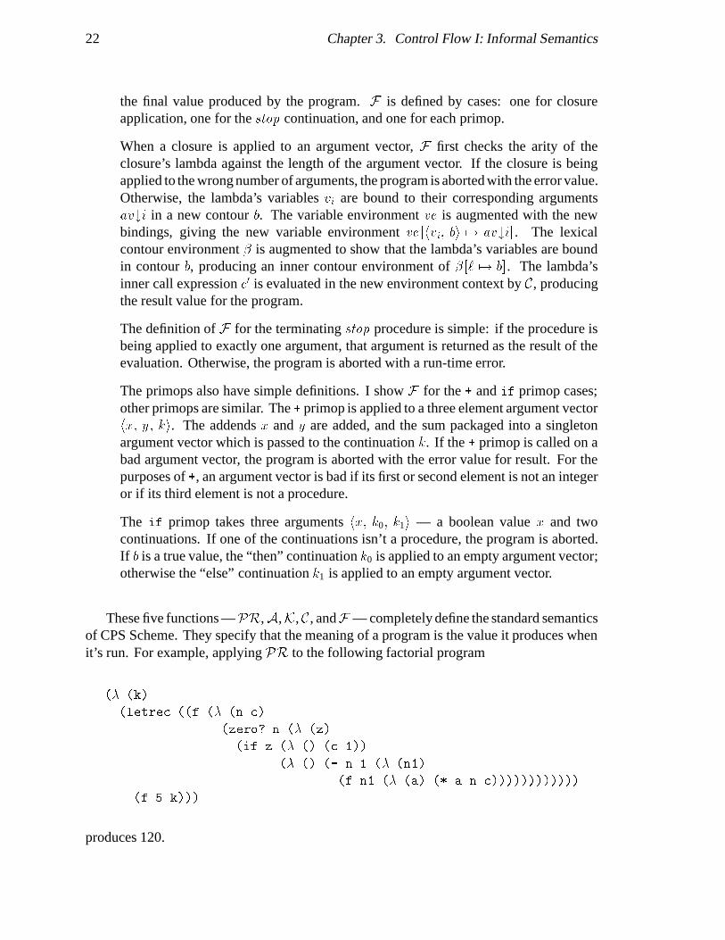
These five functions —PR,A,K, C , andF — completely define the standard semanticsof CPS Scheme. They specify that the meaning of a program is the value it produces whenit’s run. For example, applying PR to the following factorial program
(� (k)
(letrec ((f (� (n c)
(zero? n (� (z)
(if z (� () (c 1))
(� () (- n 1 (� (n1)
(f n1 (� (a) (* a n c))))))))))))
(f 5 k)))
produces 120.
3.4. Exact Control-Flow Semantics 23
3.4 Exact Control-Flow Semantics
We can derive a control-flow semantics from our standard semantics by “instrumenting theinterpreter.” We find every place in the semantics where a procedure is called, and wemodify the semantics to record the call in some table. When the program terminates, thesemantics discards the actual value computed, and returns the table instead. Our semanticsis now one that maps a program, not to its result value, but to a record of all the calls thathappened during the program execution.
Clearly, while this approach gives a well-defined mathematical definition of control-flow analysis, the definition is unrealisable as a computable algorithm. If the program neverterminates, the interpreter will never halt, and never finish constructing the table. Further,the table produced reflects only the calls that happen during one particular execution of theprogram — it captures precisely the transfers of control that take place during that execution.Suppose we had more realistically included i/o in our semantics. To get a general pictureof the program’s control-flow structure, we would have to interpret the program for eachpossible input set, and join the result tables together. These issues are not a concern fornow; we’ll worry about how to make the analysis computable later. For now, it sufficesthat our instrumented interpreter serves as a very precise, formal definition of control-flowanalysis.
3.4.1 Internal Call Sites
There is one fine point we must consider before proceeding to our control-flow se-mantics: not all procedures are called from program call sites. Consider the fragment(+ a b (� (s) (f a s))). Where is (� (s) (f a s)) called from? It is called fromthe innards of the + primop; there is no corresponding call site in the program syntax to markthis. We need to endow primops with special internal call sites to mark calls to functionsthat happen internal to the primop.
For each occurrence of a primop (p:prim a1 . . . an) in a program, we associate a relatedset of internal call sites ic1
p; . . . ; icjp for the primop’s use. Simple primops, e.g. +, have asingle internal call site, which marks the call to the primop’s continuation. Conditionalprimops, e.g. if, have two internal call sites, one for the consequent continuation, and onefor the alternate continuation. These ic identifiers give us names for the hidden call siteswhere primop continuations are called. So, we include them in the LAB set:
LAB =n`i; ri; ci; ic
jp; . . .
o:
Now our label set includes the labels of all possible call sites in the program, both visibleand hidden.
Some notational conveniences: Most ordinary primops only require a single internalcall site. When this is the case, we’ll drop the superscript index. Furthermore, whenpossible we’ll include the actual primop with its label in the subscript. So if the primopwith label p happens to be [[p:+]], we’ll write its single internal call site as icp:+ instead ofic1
p.

24 Chapter 3. Control Flow I: Informal Semantics
3.4.2 Instrumenting the Semantics
We only need to change the standard semantics slightly to produce our exact control-flowsemantics (figure 3.3). The only domain we must change is the answer domain, Ans. Ournew semantics produces call caches. A call cache ( 2 CCache) is a partial map fromcall-site/contour-environment pairs to procedures:
CCache = (LAB� BEnv) * Proc
Ans = CCache
Note that this definition of a call cache is more detailed than one that simply maps a callsite to the procedures called from that site. This definition distinguishes the multiple callsthat happen from a single call site by including the environment context (from BEnv) aspart of the input to the cache.
Figure 3.3 shows the new interpreter. Instrumenting the standard interpreter involvestwo basic changes.
1. The places where procedures are called — fromPR’s top-level call, from C’s simple-call case, and from F ’s continuation calls inside primop applications — must addtheir call to the call cache being built up by the interpretation.
2. Program termination, whether by run-time error or application of the stop continu-ation, must discard the actual result value and produce instead the empty call cache[ ].
The PR function is similar to its previous definition: it closes the top-level lambda inthe empty environment and applies it to the stop continuation. This procedure application,however, evaluates to the call cache produced by running the rest of the program. PRmust add to this cache the fact that the top-level procedure f was called from the top callin the empty environment. This is represented by the cache entry
�hctop; [ ]i 7! f
�, where
the label ctop represents the call site for the top-level call. The updated call cache is the callcache for the entire program execution.
The A function hasn’t changed at all, since evaluating argument expressions doesn’tinvolve calling procedures.
The simple-call case of the C function changes in two respects. First, in the error case,it aborts the program and returns the empty call cache [ ]. C is responsible for returning thecall cache for program execution from its call onwards; since the program has halted at thecall, the empty call cache is the right value to produce. Second, if it actually performs acall, it records the fact that procedure f 0 was called from call c in context �, represented bycall cache entry
�hc; �i 7! f 0
�. This entry is added to the call cache produced by running
the rest of the program.The letrec case doesn’t change, since the letrec’s local computation is simply a
binding operation, and doesn’t perform any procedure calls itself.The F function performs calls to its primops’ continuations, and these calls must be
recorded. For example, the + primop performs a call to its continuation k from its internal
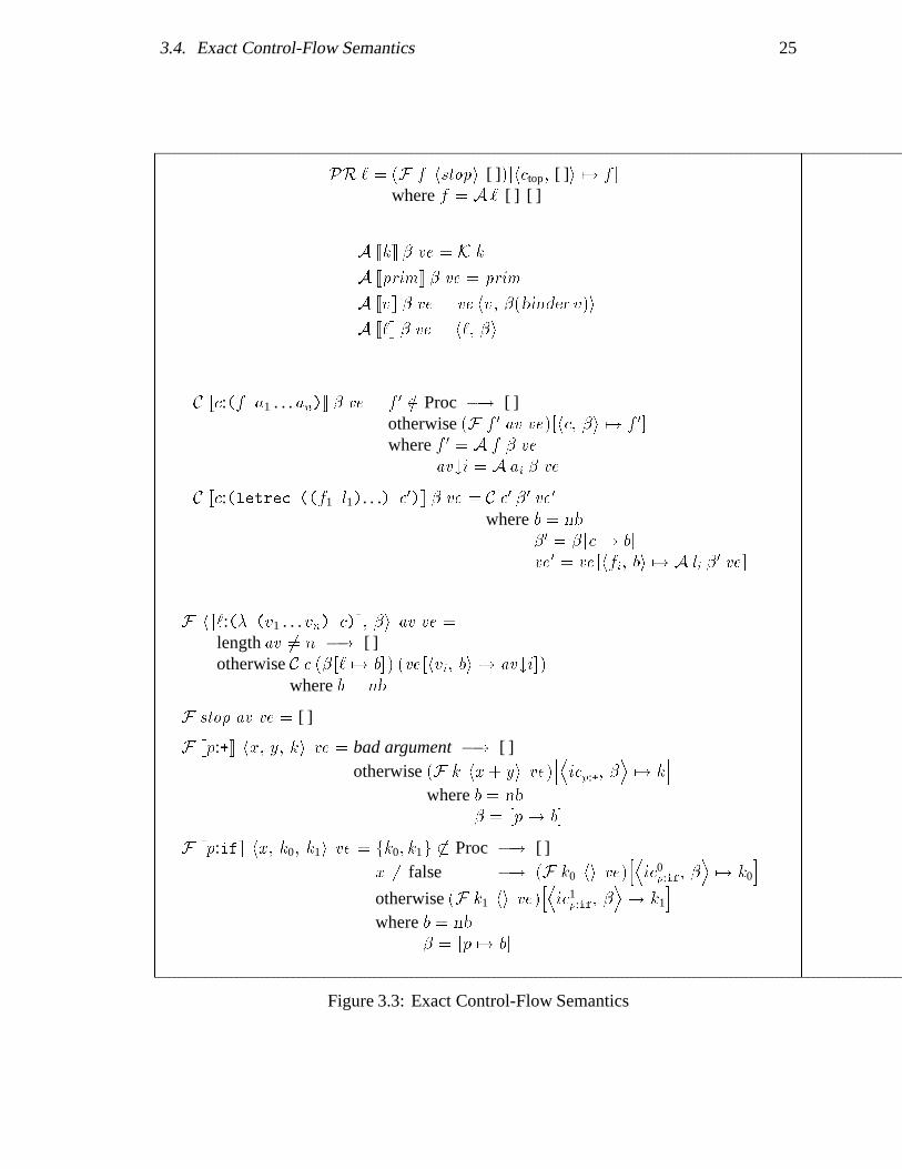
3.4. Exact Control-Flow Semantics 25
PR ` = (F f hstopi [ ])�hctop; [ ]i 7! f
�where f = A ` [ ] [ ]
A [[k]] � ve = K k
A [[prim]] � ve = prim
A [[v]] � ve = ve hv; �(binder v)i
A [[`]] � ve = h`; �i
C [[c:(f a1 . . . an)]] � ve = f 0 =2 Proc �! [ ]otherwise (F f 0
av ve)�hc; �i 7! f 0
�where f 0 = A f � ve
av#i = A ai � ve
C [[c:(letrec ((f1 l1). . .) c0)]] � ve = C c0 �0ve
0
where b = nb
�0 = ��c 7! b
�ve
0 = ve�hfi; bi 7! A li �
0ve�
F h[[`:(� (v1 . . . vn) c)]]; �i av ve =
length av 6= n �! [ ]otherwise C c (�
�` 7! b
�) (ve
�hvi; bi 7! av#i
�)
where b = nb
F stop av ve = [ ]
F [[p:+]] hx; y; ki ve = bad argument �! [ ]otherwise (F k hx+ yi ve)
hDicp:+; �
E7! k
iwhere b = nb
� =�p 7! b
�F [[p:if]] hx; k0; k1i ve = fk0; k1g 6� Proc �! [ ]
x 6= false �! (F k0 hi ve)hDic0
p:if; �E7! k0
iotherwise (F k1 hi ve)
hDic1
p:if; �E7! k1
iwhere b = nb
� =�p 7! b
�
Figure 3.3: Exact Control-Flow Semantics
26 Chapter 3. Control Flow I: Informal Semantics
call site icp:+. This is recorded by call cache entryhDicp:+; �
E7! k
iwhich is added to the
cache produced by running the rest of the program.Note that + allocates a new contour when it is entered, even though it binds no variables.
In the course of executing a program, control could pass through this primop several times;each time, there will be a call from icp:+ to a continuation. We need to distinguish thesemultiple icp:+ calls in the call cache we are constructing. Multiple calls from the same callsite are distinguished in the call cache by an environment context �. So, even though itbinds no variables, when control enters a + primop, we allocate a new contour b = nb, andconstruct a new contour environment � =
�p 7! b
�to make a unique index
Dicp:+; �
Ein the
call cache.Similarly, if adds the appropriate entry to the final call cache, either recording that the
true continuation k0 was called from the internal call site ic0p:if, or the false continuation k1
was called from ic1p:if.
3.5 Abstract Control-Flow Semantics
Now that we’ve defined our control-flow analysis semantics, we have a formal descriptionof the control-flow problem. The final step is to abstract our semantics to a computableapproximate semantics that is useful and safe.
The major reason the exact semantics is uncomputable is because the domains andranges of the meaning functions are (uncountably) infinite. This is due to the infinitenumber of distinct environments that can be created at run time.
For example, the call cache constructed by the analysis is a potentially infinite table. Ifa call cache simply mapped call sites to lambdas, it would necessarily be finite, because afinite program only has a finite number of call sites and lambdas. A call cache, however,maps call contexts to closures. The difference is environment information. A call contexthc; �i is a call paired with a contour environment; similarly, a closure h`; �i is a lambdapaired with a contour environment. Although there are only a finite number of lambdas andcalls in a given program, execution of that program can give rise to an unbounded numberof distinct environments.
For example, consider the following Scheme loop:
(letrec ((loop (� (f) (loop (� (n) (* 2 (f n)))))))
(loop (� (m) m)))
The loop procedure calls itself with a function that is its input function doubled. What isthe set of procedures that f could be bound to during execution of this loop? It could bebound to any of the procedures
fn 7! n; n 7! 2n; n 7! 4n; . . .g :
This example shows how a finite program can give rise to an infinite set of procedures.There are only a finite number of lambda expressions in a given program; the infinite sets of

3.5. Abstract Control-Flow Semantics 27
procedures arise because we can close these lambdas with an infinite set of environments.If we can collapse our infinite set of environments down to a finite approximation, then wecan successfully compute a control-flow cache function.
The source of the infinite environments are the infinite contours allocated by nb duringprogram interpretation. If we force nb to allocate contours from a finite set, then we’llonly have a finite set of contour environments to deal with. This, in turn, will restrict ouranalysis to a finite set of call contexts and closures, and our table construction will converge— giving us a computable analysis. Of course, collapsing an infinite set of binding contoursdown to a finite set is going to merge some variable bindings together — that is, lookingup a variable will produce a set of possibilities, instead of a single definite value. This isthe loss of precision we must accept for a computable abstraction.
To repeat the point: the key to making our analysis computable lies in restricting ourcontour set to be finite. This is the central abstraction of the computable analysis.
It should now be clear why we factored the environment structure from the beginning.The variable binding mechanism is what gave rise to the infinite environment structure;factoring the environment exposed this mechanism to possible abstraction. Abstracting thecontours and merging bindings was the critical step that allowed us to reduce this infinitestructure to a finite, computable one.
The other major change we must make in abstracting our semantics concerns conditionalbranches. Since we do not in general know at compile time which way a conditional branchwill go, we must abstract away conditional dependencies. The if primop now “branchesboth ways.” That is, the caches arising from the consequent and alternate paths are bothcomputed; these are joined together to give the result cache returned by the if primop.Removing this data dependency has a further consequence: because basic values (fromBas) are no longer tested by conditional branches, the basic value set can be dispensed with.Since our semantics concerns itself solely with control flow, the only values that need to beconsidered are those representing CPS Scheme procedures. (Had we included I/O in ouroriginal perfect control-flow semantics, this change would allow us to abstract away thosedependencies, as well.)
The domains and functionalities for the abstract control-flow semantics are shown infigure 3.4. The abstract domains and functions are distinguished by putting “hats” on thevariable names. Closures (dClo) are still lambda/environment pairs, but the environment isnow an abstract environment (from dBEnv). The set of run-time values (bD) has changedsignificantly. As discussed, the set of basic values (Bas) has been dropped entirely. Further,an element from bD is a set of abstract procedures instead of a single procedure, reflectingthe fact that expressions now evaluate to sets of possibilities in the abstract semantics.
We’ve only specified in figure 3.4 that the abstract contour set dCN is finite — we haven’tsaid anything about what particular finite set it is. We can choose different abstractions bychoosing different finite sets for dCN and different functions cnb for allocating its contours.These different choices have varying cost/precision tradeoffs; we’ll be considering variouspossibilities in following sections. However, the general model we are developing in thissection will apply to all of the possible choices. The important particular to keep in mindis that the infinite set of exact contours has been reduced to a finite set of abstract contours.
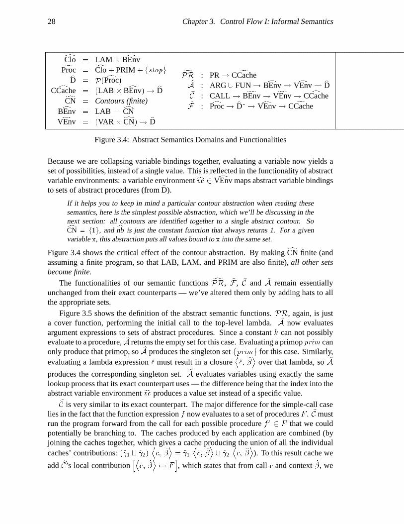
28 Chapter 3. Control Flow I: Informal Semantics
dClo = LAM � dBEnvdProc = dClo + PRIM + fstopgbD = P( dProc)dCCache = (LAB � dBEnv)! bDdCN = Contours (finite)dBEnv = LAB * dCNdVEnv = (VAR�dCN)! bD
dPR : PR ! dCCachebA : ARG [ FUN ! dBEnv ! dVEnv * bDbC : CALL ! dBEnv ! dVEnv ! dCCachebF : dProc ! bD� ! dVEnv ! dCCache
Figure 3.4: Abstract Semantics Domains and Functionalities
Because we are collapsing variable bindings together, evaluating a variable now yields aset of possibilities, instead of a single value. This is reflected in the functionality of abstractvariable environments: a variable environment cve 2 dVEnv maps abstract variable bindingsto sets of abstract procedures (from bD).
If it helps you to keep in mind a particular contour abstraction when reading thesesemantics, here is the simplest possible abstraction, which we’ll be discussing in thenext section: all contours are identified together to a single abstract contour. SodCN = f1g, and cnb is just the constant function that always returns 1. For a givenvariable x, this abstraction puts all values bound to x into the same set.
Figure 3.4 shows the critical effect of the contour abstraction. By making dCN finite (andassuming a finite program, so that LAB, LAM, and PRIM are also finite), all other setsbecome finite.
The functionalities of our semantic functions dPR, bF , bC and bA remain essentiallyunchanged from their exact counterparts — we’ve altered them only by adding hats to allthe appropriate sets.
Figure 3.5 shows the definition of the abstract semantic functions. PR, again, is justa cover function, performing the initial call to the top-level lambda. bA now evaluatesargument expressions to sets of abstract procedures. Since a constant k can not possiblyevaluate to a procedure, bA returns the empty set for this case. Evaluating a primop prim canonly produce that primop, so bA produces the singleton set fprimg for this case. Similarly,evaluating a lambda expression ` must result in a closure
D`; b�E over that lambda, so bA
produces the corresponding singleton set. bA evaluates variables using exactly the samelookup process that its exact counterpart uses — the difference being that the index into theabstract variable environment cve produces a value set instead of a specific value.bC is very similar to its exact counterpart. The major difference for the simple-call caselies in the fact that the function expression f now evaluates to a set of procedures F . bC mustrun the program forward from the call for each possible procedure f 0 2 F that we couldpotentially be branching to. The caches produced by each application are combined (byjoining the caches together, which gives a cache producing the union of all the individualcaches’ contributions: ( 1 t 2)
Dc; b�E = 1
Dc; b�E [ 2
Dc; b�E). To this result cache we
add bC’s local contributionhDc; b�E 7! F
i, which states that from call c and context b�, we
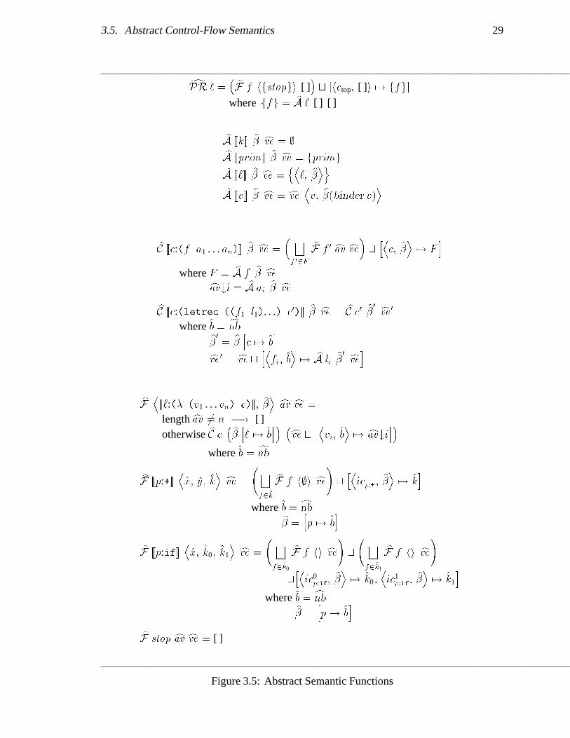
3.5. Abstract Control-Flow Semantics 29
dPR ` =� bF f hfstopgi [ ]
�t�hctop; [ ]i 7! ffg
�where ffg = bA ` [ ] [ ]
bA [[k]] b� cve = ;bA [[prim]] b� cve = fprimg
bA [[`]] b� cve =nD
`; b�EobA [[v]] b� cve = cve Dv; b�(binder v)E
bC [[c:(f a1 . . . an)]] b� cve =
� Gf 02F
bF f 0 cav cve� t hDc; b�E 7! Fi
where F = bA f b� cvecav#i = bA aib� cve
bC [[c:(letrec ((f1 l1). . .) c0)]] b� cve = bC c0 b�0 cve 0where b = cnbb�0
= b� hc 7! bi
cve 0 = cve t hDfi; bE 7! bA lib�0 cvei
bF D[[`:(� (v1 . . . vn) c)]]; b�E cav cve =
length cav 6= n �! [ ]otherwise bC c
� b� h` 7! bi� �cve t hDvi; bE 7! cav#ii�
where b = cnbbF [[p:+]]
Dx; y; k
E cve =
Gf2^k
bF f h;i cve!thDicp:+;
b�E 7! ki
where b = cnbb� =hp 7! b
i
bF [[p:if]]Dx; k0; k1
E cve =
Gf2^k0
bF f hi cve!t
Gf2^k1
bF f hi cve!
thDic0
p:if;b�E 7! k0;
Dic1
p:if;b�E 7! k1
iwhere b = cnbb� =
hp 7! b
ibF stop cav cve = [ ]
Figure 3.5: Abstract Semantic Functions

30 Chapter 3. Control Flow I: Informal Semantics
could have called any of the procedures in F . Because we are collapsing contours together,we may already have a set of procedures associated with call cache entry
Dc; b�E. This is
why the cache addition is made with a join operation, so that we are in effect adding theset of procedures F to any that we may have already recorded in the call cache under theDc; b�E entry. By not overwriting any old information we have, only adding to it, we keep
our analysis conservative.bC in the letrec case is similar to the exact version. Because we might already haveentries in the variable environment cve for the variable bindings
Dfi; b
E, we again must join
the new procedures in with the current entries to produce the new environment cve 0.bF applies an abstract procedure to a vector of value sets. If the procedure is a closureD`; b�E, the arity of the lambda is checked. If the closure is being applied to the wrong
number of arguments, the abstract interpretation is aborted, and bF returns the empty callcache [ ]. Otherwise, bF allocates an abstract contour (b = cnb) in which to bind thelambda’s variables. Just as in bC’s letrec case, the variable bindings
Dvi; b
Emight already
have entries in the variable environment cve . We add the set of values cav#i to whatevervalues we already have bound to entry
Dvi; b
Ein the variable environment cve , producing
the new environment cve t hDvi; bE 7! cav#ii. The lambda’s inner call c is evaluated in theupdated environment, giving the call cache for executing the rest of the program.
If the procedure is the + primop, the argument vector passed to it contains three values:Dx; y; k
E. The argument k is a set of possible continuations, and the abstract addends x and
y are irrelevant — they have no procedural interpretation. bF runs the interpretation forwardfor each abstract continuation f 2 k. In the exact semantics, the continuation was appliedto the sum of the primop’s addends; in the abstract semantics, we know that whatever thesum could be, it couldn’t possibly be a procedure, so its abstraction as a value set is ;. Soeach abstract continuation f is applied to the argument vector h;i. The resulting call cachesare all joined together, and +’s local contribution
hDicp:+;
b�E 7! ki
is added, which states
that all of the continuations passed in as +’s argument k could have been called from +’sinternal call site in the environment context b�.
Note that the abstract definition of the + primop does less error checking than the exactone: it doesn’t check to ensure that the addends are integer values. For example, if the exactcontrol-flow semantics was applied to the expression (+ 3 #f k), it would immediatelyhalt the interpretation, making no further entries to the call cache. The approximatesemantics, however, would record the primop’s call to the continuation, and continue theinterpretation. This is acceptable, since including some extra calls in the final call cache iserring on the conservative side – the abstract analysis hasn’t left out any of the actual calls,only included a few extras. This (conservative) weakening of the run-time error checkingis a pervasive feature of the abstract analysis.
The if primop case is similar to the + case, except that we branch both ways from theconditional.
The stop case is again quite simple: no calls are made after applying the stop procedure,so the empty call cache is returned.

3.6. 0CFA 31
3.6 0CFA
The abstract semantics of the last section didn’t specify which finite set to choose for theabstract contours dCN, or what rule to use for allocating these contours on procedure entry.In this section, we’ll look at the simplest possible abstraction, in which there is only a singleabstract contour: dCN = f1g. Thus the cnb function is just the constant function alwaysreturning 1. In the exact semantics, all bindings of a given variable were kept distinct;in this simple abstraction, all bindings of a given variable are merged together. Supposethat, over the lifetime of a program some variable x is bound to seven different values:fd1; d2; . . . ; d7g. In 0CFA, after these bindings have been made, evaluation of x in anyenvironmental context produces not one of the di, but the entire set. This trivial abstractionis called “0th-order Control-Flow Analysis” (0CFA) (we’ll consider other, more detailedabstractions in the next section).
Even though 0CFA is quite simple, it is still very useful, particularly for intra-proceduralflow analysis. For example, the implementation of induction-variable elimination discussedin chapter 7 is based on a 0CFA analysis. Additionally, 0CFA has the attraction of beingfast.
We could write down the equations for the 0CFA semantics simply by replacing “cnb”with “1” throughout the equations of the previous section. However, once we do this, wecan simplify the equations further (figures 3.6, 3.7). 0CFA is a very special abstractionbecause it is the trivial case. Many of the structures in the general abstract semanticscollapse to degenerate cases in 0CFA. For example, once we specify that dCN = f1g, thencontour environments become degenerate: every environment � maps all its labels to 1.So we can dispose of contour environments in the special case of 0CFA. Similarly, thevariable/contour pairs hv; bi that index variable environments become degenerate, sincethe contour, again, must always be 1. So, we can simplify the variable environment domainto be maps from variables to sets of values: VAR ! bD. The same reasoning applies toclosures and call caches: the context information � that is paired with a lambda ` to makea closure, and paired with a call to make a call cache index is degenerate. So we canrepresent an abstract procedure with just a lambda, and a call cache now maps calls to setsof lambdas.
dProc = LAM + PRIM + fstopgbD = P( dProc)dCCache = LAB ! bDdVEnv = VAR ! bD
dPR : PR ! dCCachebA : ARG [ FUN ! dVEnv * bDbC : CALL ! dVEnv ! dCCachebF : dProc ! bD� ! dVEnv ! dCCache
Figure 3.6: 0CFA Domains and Functionalities
The 0CFA analysis is interesting because it analyses pure control-flow structure; envi-ronment structure is ignored completely. It provides a direct answer to the question “Whichlambdas are called from which call sites?” Because it is so simple, it can be computed fasterthan other, more detailed abstractions. However, the simplicity carries a price of reduced
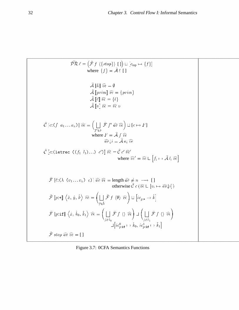
32 Chapter 3. Control Flow I: Informal Semantics
dPR ` =� bF f hfstopgi [ ]
�t�ctop 7! ffg
�where ffg = bA ` [ ]
bA [[k]] cve = ;bA [[prim]] cve = fprimgbA [[`]] cve = f`gbA [[v]] cve = cve v
bC [[c:(f a1 . . . an)]] cve =
� Gf 02F
bF f 0 cav cve� t [c 7! F ]
where F = bA f cvecav#i = bA ai cvebC [[c:(letrec ((f1 l1). . .) c0)]] cve = bC c0 cve 0
where cve 0 = cve t hfi 7! bA li cvei
bF [[`:(� (v1 . . . vn) c)]] cav cve = length cav 6= n �! [ ]otherwise bC c (cve t �vi 7! cav#i�)
bF [[p:+]]Dx; y; k
E cve =
Gf2^k
bF f h;i cve!thicp:+ 7! k
i
bF [[p:if]]Dx; k0; k1
E cve =
Gf2^k0
bF f hi cve!t
Gf2^k1
bF f hi cve!
thic0
p:if 7! k0; ic1p:if 7! k1
ibF stop cav cve = [ ]
Figure 3.7: 0CFA Semantics Functions
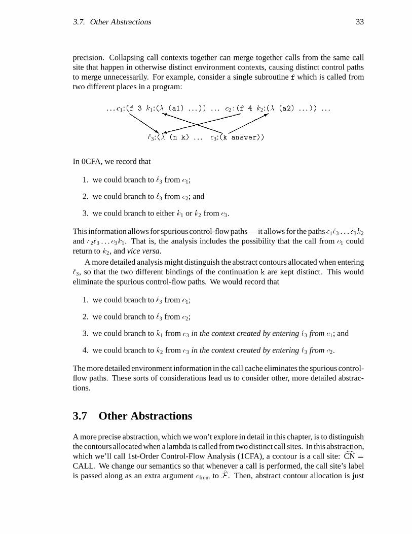
3.7. Other Abstractions 33
precision. Collapsing call contexts together can merge together calls from the same callsite that happen in otherwise distinct environment contexts, causing distinct control pathsto merge unnecessarily. For example, consider a single subroutine f which is called fromtwo different places in a program:
. . . c1:(f 3 k1:(� (a1) . . . )) . . . c2:(f 4 k2:(� (a2) . . . )) . . .
`3:(� (n k) . . . c3:(k answer))������*
PPPPPPPPPi ������������9
QQQQQs
In 0CFA, we record that
1. we could branch to `3 from c1;
2. we could branch to `3 from c2; and
3. we could branch to either k1 or k2 from c3.
This information allows for spurious control-flow paths — it allows for the paths c1`3 . . . c3k2
and c2`3 . . . c3k1. That is, the analysis includes the possibility that the call from c1 couldreturn to k2, and vice versa.
A more detailed analysis might distinguish the abstract contours allocated when entering`3, so that the two different bindings of the continuation k are kept distinct. This wouldeliminate the spurious control-flow paths. We would record that
1. we could branch to `3 from c1;
2. we could branch to `3 from c2;
3. we could branch to k1 from c3 in the context created by entering `3 from c1; and
4. we could branch to k2 from c3 in the context created by entering `3 from c2.
The more detailed environment information in the call cache eliminates the spurious control-flow paths. These sorts of considerations lead us to consider other, more detailed abstrac-tions.
3.7 Other Abstractions
A more precise abstraction, which we won’t explore in detail in this chapter, is to distinguishthe contours allocated when a lambda is called from two distinct call sites. In this abstraction,which we’ll call 1st-Order Control-Flow Analysis (1CFA), a contour is a call site: dCN =
CALL. We change our semantics so that whenever a call is performed, the call site’s labelis passed along as an extra argument cfrom to bF . Then, abstract contour allocation is just
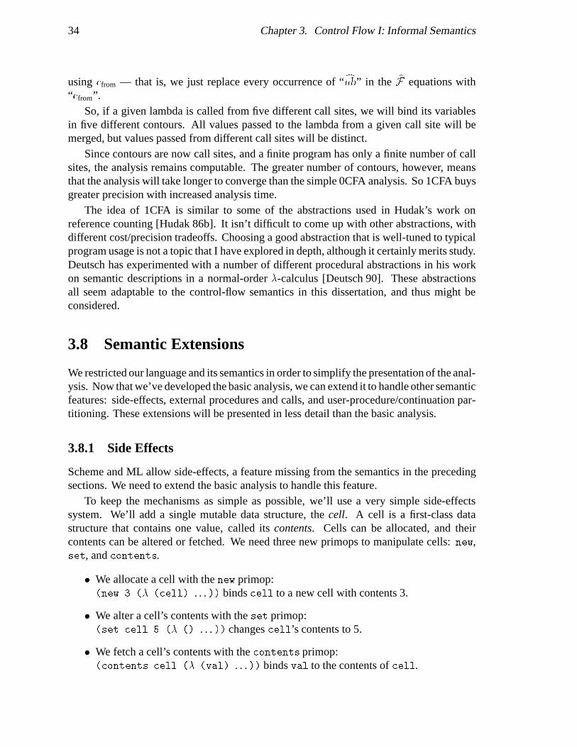
34 Chapter 3. Control Flow I: Informal Semantics
using cfrom — that is, we just replace every occurrence of “cnb” in the bF equations with“cfrom”.
So, if a given lambda is called from five different call sites, we will bind its variablesin five different contours. All values passed to the lambda from a given call site will bemerged, but values passed from different call sites will be distinct.
Since contours are now call sites, and a finite program has only a finite number of callsites, the analysis remains computable. The greater number of contours, however, meansthat the analysis will take longer to converge than the simple 0CFA analysis. So 1CFA buysgreater precision with increased analysis time.
The idea of 1CFA is similar to some of the abstractions used in Hudak’s work onreference counting [Hudak 86b]. It isn’t difficult to come up with other abstractions, withdifferent cost/precision tradeoffs. Choosing a good abstraction that is well-tuned to typicalprogram usage is not a topic that I have explored in depth, although it certainly merits study.Deutsch has experimented with a number of different procedural abstractions in his workon semantic descriptions in a normal-order �-calculus [Deutsch 90]. These abstractionsall seem adaptable to the control-flow semantics in this dissertation, and thus might beconsidered.
3.8 Semantic Extensions
We restricted our language and its semantics in order to simplify the presentation of the anal-ysis. Now that we’ve developed the basic analysis, we can extend it to handle other semanticfeatures: side-effects, external procedures and calls, and user-procedure/continuation par-titioning. These extensions will be presented in less detail than the basic analysis.
3.8.1 Side Effects
Scheme and ML allow side-effects, a feature missing from the semantics in the precedingsections. We need to extend the basic analysis to handle this feature.
To keep the mechanisms as simple as possible, we’ll use a very simple side-effectssystem. We’ll add a single mutable data structure, the cell. A cell is a first-class datastructure that contains one value, called its contents. Cells can be allocated, and theircontents can be altered or fetched. We need three new primops to manipulate cells: new,set, and contents.
� We allocate a cell with the new primop:(new 3 (� (cell) . . . )) binds cell to a new cell with contents 3.
� We alter a cell’s contents with the set primop:(set cell 5 (� () . . . )) changes cell’s contents to 5.
� We fetch a cell’s contents with the contents primop:(contents cell (� (val) . . .)) binds val to the contents of cell.
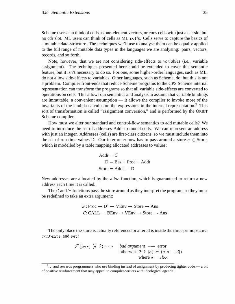
3.8. Semantic Extensions 35
Scheme users can think of cells as one-element vectors, or cons cells with just a car slot butno cdr slot. ML users can think of cells as ML ref’s. Cells serve to capture the basics ofa mutable data-structure. The techniques we’ll use to analyse them can be equally appliedto the full range of mutable data types in the languages we are analysing: pairs, vectors,records, and so forth.
Note, however, that we are not considering side-effects to variables (i.e., variableassignment). The techniques presented here could be extended to cover this semanticfeature, but it isn’t necessary to do so. For one, some higher-order languages, such as ML,do not allow side-effects to variables. Other languages, such as Scheme, do; but this is nota problem. Compiler front-ends that reduce Scheme programs to the CPS Scheme internalrepresentation can transform the programs so that all variable side-effects are converted tooperations on cells. This allows our semantics and analysis to assume that variable bindingsare immutable, a convenient assumption — it allows the compiler to invoke more of theinvariants of the lambda-calculus on the expressions in the internal representation.2 Thissort of transformation is called “assignment conversion,” and is performed by the ORBIT
Scheme compiler.How must we alter our standard and control-flow semantics to add mutable cells? We
need to introduce the set of addresses Addr to model cells. We can represent an addresswith just an integer. Addresses (cells) are first-class citizens, so we must include them intothe set of run-time values D. Our interpreter now has to pass around a store � 2 Store,which is modelled by a table mapping allocated addresses to values:
Addr = Z
D = Bas + Proc + Addr
Store = Addr * D
New addresses are allocated by the alloc function, which is guaranteed to return a newaddress each time it is called.
The C andF functions pass the store around as they interpret the program, so they mustbe redefined to take an extra argument:
F : Proc ! D�! VEnv ! Store ! Ans
C: CALL ! BEnv ! VEnv ! Store ! Ans
The only place the store is actually referenced or altered is inside the three primops new,contents, and set:
F [[new]] hd; ki ve � = bad argument �! errorotherwise F k hai ve (�
�a 7! d
�)
where a = alloc
2. . . and rewards programmers who use binding instead of assignment by producing tighter code — a bitof positive reinforcement that may appeal to compiler-writers with ideological agenda.
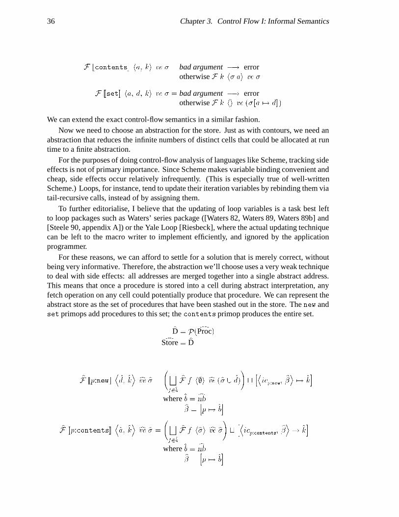
36 Chapter 3. Control Flow I: Informal Semantics
F [[contents]] ha; ki ve � = bad argument �! errorotherwise F k h� ai ve �
F [[set]] ha; d; ki ve � = bad argument �! errorotherwise F k hi ve (�
�a 7! d
�)
We can extend the exact control-flow semantics in a similar fashion.Now we need to choose an abstraction for the store. Just as with contours, we need an
abstraction that reduces the infinite numbers of distinct cells that could be allocated at runtime to a finite abstraction.
For the purposes of doing control-flow analysis of languages like Scheme, tracking sideeffects is not of primary importance. Since Scheme makes variable binding convenient andcheap, side effects occur relatively infrequently. (This is especially true of well-writtenScheme.) Loops, for instance, tend to update their iteration variables by rebinding them viatail-recursive calls, instead of by assigning them.
To further editorialise, I believe that the updating of loop variables is a task best leftto loop packages such as Waters’ series package ([Waters 82, Waters 89, Waters 89b] and[Steele 90, appendix A]) or the Yale Loop [Riesbeck], where the actual updating techniquecan be left to the macro writer to implement efficiently, and ignored by the applicationprogrammer.
For these reasons, we can afford to settle for a solution that is merely correct, withoutbeing very informative. Therefore, the abstraction we’ll choose uses a very weak techniqueto deal with side effects: all addresses are merged together into a single abstract address.This means that once a procedure is stored into a cell during abstract interpretation, anyfetch operation on any cell could potentially produce that procedure. We can represent theabstract store as the set of procedures that have been stashed out in the store. The new andset primops add procedures to this set; the contents primop produces the entire set.
bD = P( dProc)dStore = bD
bF [[p:new]]Dd; k
E cve b� =
Gf2^k
bF f h;i cve (b� [ d)
!t
hDicp:new;
b�E 7! ki
where b = cnbb� =hp 7! b
i
bF [[p:contents]]Da; k
E cve b� =
Gf2^k
bF f hb�i cve b�!thDicp:contents;
b�E 7! ki
where b = cnbb� =hp 7! b
i
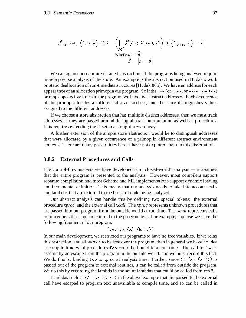
3.8. Semantic Extensions 37
bF [[p:set]]Da; d; k
E cve b� =
Gf2^k
bF f hi cve (b� [ d)
!thDicp:set;
b�E 7! ki
where b = cnbb� =hp 7! b
i
We can again choose more detailed abstractions if the programs being analysed requiremore a precise analysis of the store. An example is the abstraction used in Hudak’s workon static deallocation of run-time data structures [Hudak 86b]. We have an address for eachappearance of an allocation primop in our program. So if thenew (orcons, ormake-vector)primop appears five times in the program, we have five abstract addresses. Each occurrenceof the primop allocates a different abstract address, and the store distinguishes valuesassigned to the different addresses.
If we choose a store abstraction that has multiple distinct addresses, then we must trackaddresses as they are passed around during abstract interpretation as well as procedures.This requires extending the bD set in a straightforward way.
A further extension of the simple store abstraction would be to distinguish addressesthat were allocated by a given occurrence of a primop in different abstract environmentcontexts. There are many possibilities here; I have not explored them in this dissertation.
3.8.2 External Procedures and Calls
The control-flow analysis we have developed is a “closed-world” analysis — it assumesthat the entire program is presented to the analysis. However, most compilers supportseparate compilation and most Scheme and ML implementations support dynamic loadingand incremental definition. This means that our analysis needs to take into account callsand lambdas that are external to the block of code being analysed.
Our abstract analysis can handle this by defining two special tokens: the externalprocedure xproc, and the external call xcall. The xproc represents unknown procedures thatare passed into our program from the outside world at run time. The xcall represents callsto procedures that happen external to the program text. For example, suppose we have thefollowing fragment in our program:
(foo (� (k) (k 7)))
In our main development, we restricted our programs to have no free variables. If we relaxthis restriction, and allow foo to be free over the program, then in general we have no ideaat compile time what procedures foo could be bound to at run time. The call to foo isessentially an escape from the program to the outside world, and we must record this fact.We do this by binding foo to xproc at analysis time. Further, since (� (k) (k 7)) ispassed out of the program to external routines, it can be called from outside the program.We do this by recording the lambda in the set of lambdas that could be called from xcall.
Lambdas such as (� (k) (k 7)) in the above example that are passed to the externalcall have escaped to program text unavailable at compile time, and so can be called in
38 Chapter 3. Control Flow I: Informal Semantics
arbitrary, unobservable ways. They have escaped close scrutiny, and in the face of limitedinformation, we are forced simply to assume the worst. We maintain a set ESCAPED ofescaped procedures, which initially contains xproc and the top-level lambda of the program.The rules for the external call, the external procedure and escaped functions are simple:
1. Any procedure passed to the external procedure escapes.
2. Any escaped procedure can be called from the external call.
3. When a procedure is called from the external call, it may be applied to any escapedprocedure.
This provides very weak information, but for external procedures whose properties arecompletely unknown at compile time, it is the best we can do. (On the other hand, manyexternal procedures, e.g. print, or length, have well known properties. For instance,both print and length only call their continuations. Thus, their continuations do notproperly escape. Nor are their continuations passed escaped procedures as arguments. It isstraightforward to extend the analysis presented here to utilise this stronger information.)
These rules can be easily integrated into our abstract semantics.External procedures can potentially access the store, so these two semantic features
interact. Suppose we choose the simple store abstraction discussed in the previous section.
� Any procedure placed in the abstract store can be accessed by external proceduresthat can reference the store.
� Therefore, any procedure placed in the abstract store can escape.
� Any escaping procedure can be placed in the abstract store by an external procedure.
So, given the simple store abstraction, it makes sense to identify the ESCAPED set andthe abstract store set b�, since any element that is placed in one of these sets must also beplaced in the other. (On the other hand, if we choose a more complex store abstraction, wewould want to separate these two sets, since not all abstract addresses escape, and so notall elements of the abstract store are accessible by external procedures.)
3.8.3 Partitioning Procedures and Continuations
A worthwhile enhancement of the basic semantics is to distinguish user procedures fromcontinuations.
CPS Scheme is an intermediate representation for full Scheme. In full Scheme, the usercannot write CPS-level continuations: all continuations, all variables bound to continua-tions, and all calls to continuations (i.e., returns) are introduced by the CPS converter. Thisdivides the procedural world into two halves: user procedures and continuations introducedby the CPS converter. It is easy for the CPS converter to mark these continuation lambdas,variables and call sites as it introduces them into the program. This partition is a powerful

3.8. Semantic Extensions 39
constraint on the sets propagated around by the analysis: a given call site either only callsuser procedures, or only calls continuations; a given variable is either bound to only userprocedures, or bound to only continuations. This partition holds throughout all details ofthe CFA semantics; exploiting it produces a much tighter analysis.
Distinguishing user procedures and continuations is useful for reasons besides improvingthe data-flow analysis; both ORBIT and Kelsey’s transformational compiler do some formof this marking [Kranz+ 86, Kelsey 89].
Note that this change doesn’t alter the meaning of either user procedures or continuations— in CPS Scheme they both have the meaning of a continuation procedure. We are simplyable to statically partition the procedural world into two disjoint sets, with consequentimprovements in the precision and efficiency of our analysis. In this way, a CPS-basedrepresentation lets us “have it both ways”: We can distinguish procedure calls and returnswhen it is useful to do so, and still enjoy the advantages of a unified representation andsemantics, treating all lambdas identically when convenient.
The user-procedure/continuation partition interacts with the external call mechanisms.Instead of having a value xproc to represent external procedures, we need to provide bothfor external user-level procedures xproc and external continuations xcont. Similarly, weneed to have both an external call xcall for calls to user-level procedures, and an externalreturn xret to mark calls to continuations. The extensions to handle this are straightforward.
A criteria to separate user procedures and continuation procedures is whether or not theprocedure takes a continuation argument itself. A user procedure is always called with anextra continuation argument to which it is to deliver its result. This implicit continuationis made an explicit parameter by the CPS conversion process, which introduces the extraargument into the procedure’s formal parameter list and into all the calls to the procedure.A continuation, on the other hand, completely encapsulates the computational future of aprocess, so it requires no continuation argument itself.
It is an interesting feature of this partition that source-to-source transformations on aCPS Scheme program can convert a user procedure to a continuation and vice versa. Forexample, consider the following Scheme summation loop:
(� (n)
(letrec ((lp (� (i sum)
(if (zero? i) sum (lp (- i 1) (+ sum i))))))
(lp n 0)))
If we partially CPS-convert this loop, introducing continuation variables, calls, and lambdas,we get:
(� (n k)
(letrec ((lp (� (i sum c)
(if (zero? i) (c sum)
(lp (- i 1) (+ sum i) c)))))
(lp n 0 k)))
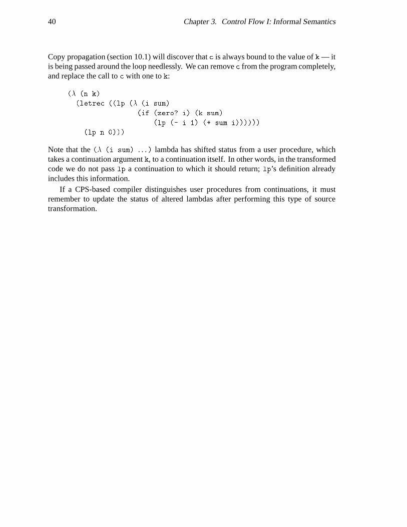
40 Chapter 3. Control Flow I: Informal Semantics
Copy propagation (section 10.1) will discover that c is always bound to the value of k — itis being passed around the loop needlessly. We can remove c from the program completely,and replace the call to c with one to k:
(� (n k)
(letrec ((lp (� (i sum)
(if (zero? i) (k sum)
(lp (- i 1) (+ sum i))))))
(lp n 0)))
Note that the (� (i sum) . . .) lambda has shifted status from a user procedure, whichtakes a continuation argument k, to a continuation itself. In other words, in the transformedcode we do not pass lp a continuation to which it should return; lp’s definition alreadyincludes this information.
If a CPS-based compiler distinguishes user procedures from continuations, it mustremember to update the status of altered lambdas after performing this type of sourcetransformation.
Chapter 4
Control Flow II: Detailed Semantics
That which must be provedcannot be worth much.
— fortune cookie,by way of Robert Harper
The aim of the previous chapter was to develop a simple semantically-based definition ofcontrol-flow analysis, along with safe, computable abstractions for it. The developmentwas kept simple for the sake of intuitive explication; the rigorous details of the necessarymathematical machinery were intentionally glossed over in order to get the “big picture”across.
Of course, one of the big attractions of defining an analysis with a denotational semanticsis that we can then rigorously prove properties about our analysis. In this chapter, I willredevelop the semantics with enough precision and care to allow us to prove some importantbasic properties of the analysis. The major results will be to show that
� The equations defining the exact and abstract control-flow semantics have solutions.
� The abstract semantics safely approximates the exact semantics.
� The abstract semantics is computable.
This is what we need to show to put the computable control-flow analysis on a firmtheoretical foundation. If you are uncomfortablewith or unwilling to read detailed semanticsproofs, you can simply take these three results on faith and skip to the next chapter.
The rest of the chapter follows this agenda:
1. First, we will change the simple equations given in the previous chapter to patch upsome holes in the definitions. For example, we will add side-effects and a store, andrestrict the domains of some functions to make them well-defined. (Section 4.1)
2. Next, we will show that the semantic functions (PR, A, C , F and their abstractcounterparts) exist. This requires showing that the recursive definitions are well-defined and have solutions. (Section 4.3)
41
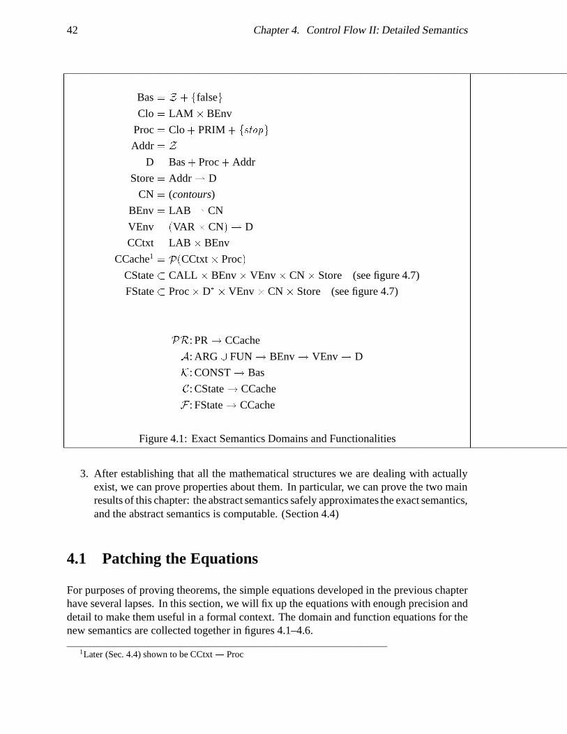
42 Chapter 4. Control Flow II: Detailed Semantics
Bas = Z + ffalseg
Clo = LAM� BEnv
Proc = Clo + PRIM + fstopg
Addr = Z
D = Bas + Proc + Addr
Store = Addr * D
CN = (contours)
BEnv = LAB * CN
VEnv = (VAR� CN) * D
CCtxt = LAB� BEnv
CCache1 = P(CCtxt� Proc)
CState � CALL � BEnv� VEnv� CN� Store (see figure 4.7)
FState � Proc� D��VEnv � CN � Store (see figure 4.7)
PR: PR ! CCache
A: ARG [ FUN ! BEnv ! VEnv * D
K: CONST ! Bas
C: CState ! CCache
F : FState ! CCache
Figure 4.1: Exact Semantics Domains and Functionalities
3. After establishing that all the mathematical structures we are dealing with actuallyexist, we can prove properties about them. In particular, we can prove the two mainresults of this chapter: the abstract semantics safely approximates the exact semantics,and the abstract semantics is computable. (Section 4.4)
4.1 Patching the Equations
For purposes of proving theorems, the simple equations developed in the previous chapterhave several lapses. In this section, we will fix up the equations with enough precision anddetail to make them useful in a formal context. The domain and function equations for thenew semantics are collected together in figures 4.1–4.6.
1Later (Sec. 4.4) shown to be CCtxt* Proc

4.1. Patching the Equations 43
PR ` = F hf; hstopi; [ ]; b0; [ ]i [ hhctop; [ ]i; fiwhere f = A ` [ ] [ ]
A [[k]] � ve = K k
A [[prim]] � ve = prim
A [[v]] � ve = ve hv; �(binder v)i
A [[`]] � ve = h`; �i
C h[[c:(f a1 . . . an)]]; �; ve ; b; �i = f 0 =2 Proc �! [ ]otherwise fhhc; �i; f 0ig [ F hf 0; av ; ve; b0; �i
where f 0 = A f � ve
av#i = A ai � ve
b0 = nb b c
C h[[c:(letrec ((f1 l1). . .) c0)]]; �; ve ; b; �i = C hc0; �0; ve 0; b0; �i
where b0 = nb b c
�0 = ��c 7! b0
�ve
0 = ve�hfi; b
0i 7! A li �0ve�
Figure 4.2: Exact Semantic Functions (a)
4.1.1 Contour Allocation
Whenever control enters a lambda, a new contour is allocated to bind its variables to theirarguments. In the previous chapter, we swept this contour allocation under the rug with thenb “gensym” function that returned a new contour each time it was called. Such a function isobviously not well-defined. In the detailed semantics, we add a “contour counter” argumentto the F and C functions. This value is a contour that is an upper bound for all the currentlyallocated contours. The nb function is defined to increment this counter. Whenever a newcontour is needed, the current contour counter is used, and nb called to generate the newbound.
Using terms like “counter” and “upper bound” means the contour set CN must be apartial order and nb must be an increasing function. Sequentially applying nb to successivecontours is essentially moving up chains in the partial order of CN. This gives us thatif the current contour b is � all allocated contours, then nb b is > all allocated contours.This is necessary for the exact semantics (both standard and control flow) to be a correctspecification of CPS Scheme. We’ll also assume there is designated initial contour b0 thatis used by the PR function to start the interpretation.
The C and F functions adhere to the following invariant as they pass around the contourcounter:
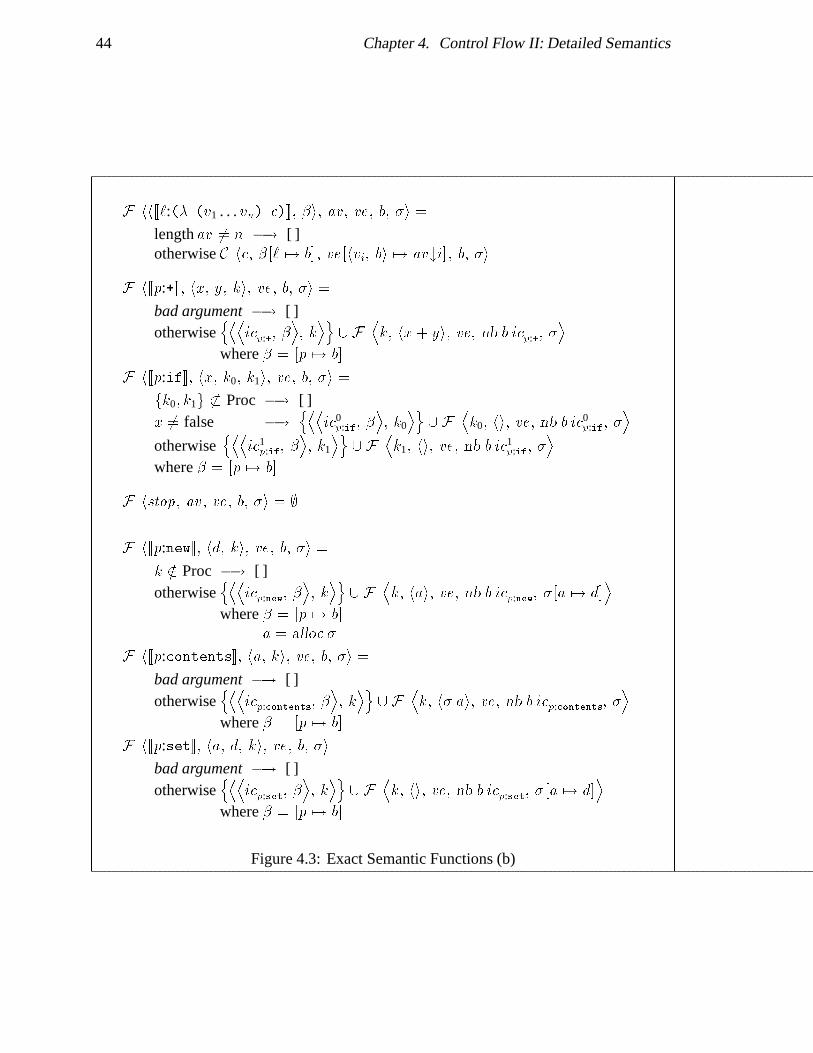
44 Chapter 4. Control Flow II: Detailed Semantics
F hh[[`:(� (v1 . . . vn) c)]]; �i; av ; ve ; b; �i =
lengthav 6= n �! [ ]otherwise C hc; �
�` 7! b
�; ve
�hvi; bi 7! av#i
�; b; �i
F h[[p:+]]; hx; y; ki; ve ; b; �i =
bad argument �! [ ]otherwise
nDDicp:+; �
E; kEo[ F
Dk; hx+ yi; ve; nb b icp:+; �
Ewhere � =
�p 7! b
�F h[[p:if]]; hx; k0; k1i; ve ; b; �i =
fk0; k1g 6� Proc �! [ ]x 6= false �!
nDDic0
p:if; �E; k0
Eo[ F
Dk0; hi; ve ; nb b ic0
p:if; �E
otherwisenDD
ic1p:if; �
E; k1
Eo[ F
Dk1; hi; ve ; nb b ic1
p:if; �E
where � =�p 7! b
�F hstop; av ; ve ; b; �i = ;
F h[[p:new]]; hd; ki; ve ; b; �i =
k =2 Proc �! [ ]otherwise
nDDicp:new; �
E; kEo[ F
Dk; hai; ve ; nb b icp:new; �
�a 7! d
�Ewhere � =
�p 7! b
�a = alloc �
F h[[p:contents]]; ha; ki; ve; b; �i =
bad argument �! [ ]otherwise
nDDicp:contents; �
E; kEo[ F
Dk; h� ai; ve ; nb b icp:contents; �
Ewhere � =
�p 7! b
�F h[[p:set]]; ha; d; ki; ve ; b; �i =
bad argument �! [ ]otherwise
nDDicp:set; �
E; kEo[ F
Dk; hi; ve; nb b icp:set; �
�a 7! d
�Ewhere � =
�p 7! b
�
Figure 4.3: Exact Semantic Functions (b)

4.1. Patching the Equations 45
dClo = LAM � dBEnvdProc = dClo + PRIM + fstopgbD = P( dProc)dStore = P( dProc)dCN = LAB (for 1CFA)
f1g (for 0CFA)dBEnv = LAB * dCNdVEnv = (VAR�dCN)! bDdCCtxt = LAB � dBEnvdCCache = (LAB � dBEnv)! bDdCState � CALL � dBEnv � dVEnv�dCN� dStore (see figure 4.8)dFState � dProc� bD�� dVEnv�dCN� dStore (see figure 4.8)
dPR: PR ! dCCachebA: ARG [ FUN ! dBEnv ! dVEnv * bDbC: dCState ! dCCachebF : dFState ! dCCache
Figure 4.4: Abstract Semantics Domains and Functionalities
� The contour passed to C is the greatest contour that has been used to date.
� The contour passed to F is a contour that has never been used.
This particular convention is the right one for the eventual 1CFA abstraction we are goingto make.
We could definenb as a simple function mapping contours to contours, with functionalityCN ! CN. However, when we abstract the semantics, we’ll be mapping these contours toabstract contours that can contain information about the dynamic behaviour of the program.For example, in 1CFA, the abstract contour allocated for entering a given lambda is the callfrom which we entered the lambda. It will help in establishing a connection between theexact and abstract semantics if we build this information into the exact contour from thebeginning. We can do this by providing extra information to the nb function:
bi+1 = nb bi x:
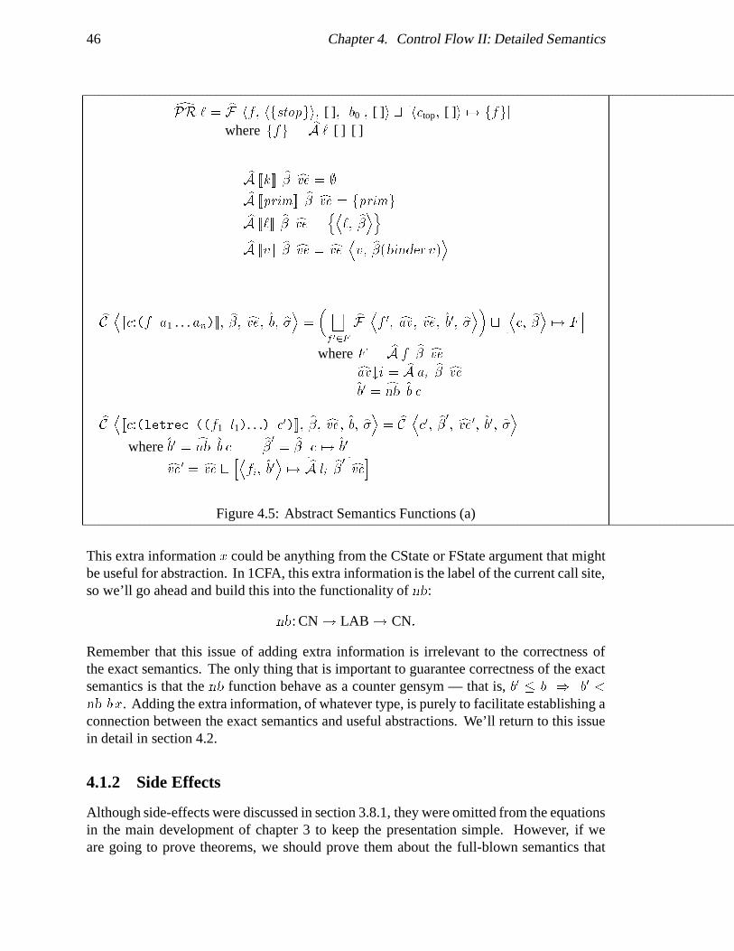
46 Chapter 4. Control Flow II: Detailed Semantics
dPR ` = bF hf; hfstopgi; [ ]; jb0j; [ ]i t�hctop; [ ]i 7! ffg
�where ffg = bA ` [ ] [ ]
bA [[k]] b� cve = ;bA [[prim]] b� cve = fprimg
bA [[`]] b� cve =nD
`; b�EobA [[v]] b� cve = cve Dv; b�(binder v)E
bC D[[c:(f a1 . . . an)]]; b�; cve ; b; b�E =
� Gf 02F
bF Df 0; cav ; cve ; b0; b�E� t hDc; b�E 7! F
i
where F = bA f b� cvecav#i = bA ai b� cveb0 = cnb b c
bC D[[c:(letrec ((f1 l1). . .) c0)]]; b�; cve ; b; b�E = bC Dc0; b�0
; cve 0; b0; b�Ewhere b0 = cnb b c b�0
= b� hc 7! b0i
cve 0 = cve t hDfi; b0E 7! bA lib�0 cvei
Figure 4.5: Abstract Semantics Functions (a)
This extra information x could be anything from the CState or FState argument that mightbe useful for abstraction. In 1CFA, this extra information is the label of the current call site,so we’ll go ahead and build this into the functionality of nb:
nb: CN ! LAB ! CN:
Remember that this issue of adding extra information is irrelevant to the correctness ofthe exact semantics. The only thing that is important to guarantee correctness of the exactsemantics is that the nb function behave as a counter gensym — that is, b0 � b ) b0 <
nb bx. Adding the extra information, of whatever type, is purely to facilitate establishing aconnection between the exact semantics and useful abstractions. We’ll return to this issuein detail in section 4.2.
4.1.2 Side Effects
Although side-effects were discussed in section 3.8.1, they were omitted from the equationsin the main development of chapter 3 to keep the presentation simple. However, if weare going to prove theorems, we should prove them about the full-blown semantics that
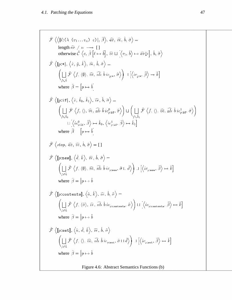
4.1. Patching the Equations 47
bF DD[[`:(� (v1 . . . vn) c)]]; b�E; cav ; cve ; b; b�E =
length cav 6= n �! [ ]otherwise bC Dc; b� h` 7! b
i; cve t hDvi; bE 7! cav#ii; b; b�E
bF D[[p:+]];
Dx; y; k
E; cve; b; b�E = G
f2k
bF Df; h;i; cve; cnb b icp:+; b�E
!thDicp:+;
b�E 7! ki
where b� =hp 7! b
i
bF D[[p:if]];
Dx; k0; k1
E; cve ; b; b�E = G
f2k0
bF Df; hi; cve; cnb b ic0
p:if; b�E!t
Gf2k1
bF Df; hi; cve; cnb b ic1
p:if; b�E!
thDic0
p:if;b�E 7! k0;
Dic1
p:if;b�E 7! k1
iwhere b� =
hp 7! b
i
bF Dstop; cav ; cve ; b; b�E = [ ]
bF D[[p:new]];
Dd; k
E; cve ; b; b�E = G
f2k
bF Df; h;i; cve; cnb b icp:new; b� t d
E!thDicp:new;
b�E 7! ki
where b� =hp 7! b
i
bF D[[p:contents]];
Da; k
E; cve ; b; b�E = G
f2k
bF Df; hb�i; cve ; cnb b icp:contents; b�E
!thDicp:contents;
b�E 7! ki
where b� =hp 7! b
i
bF D[[p:set]];
Da; d; k
E; cve; b; b�E = G
f2k
bF Df; hi; cve; cnb b icp:set; b� t d
E!thDicp:set;
b�E 7! ki
where b� =hp 7! b
i
Figure 4.6: Abstract Semantics Functions (b)
48 Chapter 4. Control Flow II: Detailed Semantics
a real CPS-based compiler for Scheme or ML would have to deal with, and this meansside-effects.
We can bring over the machinery developed in section 3.8.1 directly. The only detail notdealt with in section 3.8.1 is how unused addresses are allocated by the alloc function. Thealloc function can pick an unused address either by incrementing some external counterthat bounds the set of currently allocated addresses, or by simply choosing an address thatis not in the domain of the partial function which is the current store. The second choicerequires less machinery, so it is the one we’ll adopt:
alloc: Store ! Addr:
The critical property we require of alloc is that it allocate an unused address:
alloc � =2 Dom(�):
As discussed in section 3.8.1, there are several possibilities for store abstractions. Theone we’ll use is the simplest: all exact addresses are abstracted to a single abstract address;an abstract store is just the set of values that have been placed into the store.
4.1.3 Restricting the Function Domains
The C function takes five (curried) arguments: C c� ve b�. These are the call expression, thecontour environment, the variable environment, the contour counter, and the store. How-ever, we cannot just apply C to any five arguments chosen arbitrarily from the correspondingsets. The five arguments are all delicately intertwined and interdependent.
For example, we cannot evaluate the call c = [[(f 3)]] in an empty environment� = [ ] ; ve = [ ] — the variable lookup A [[f]] � ve would not be defined. In order tosuccessfully perform variable references while evaluating a call, the three arguments c, �,and ve must be consistent with each other.
Definition 1 c, �, ve are consistent in program P if
� Dom(�) is c’s lexical context: for every lambda or letrec ` that is lexically superiorto c (i.e., c appears in the lexical scope of `), ` 2 Dom(�).
� ve covers �: 8` 2 Dom(�) 8v 3 binder v = ` hv; �`i 2 Dom(ve).That is, all variable lookups that can be done through � are defined by ve.
This definition of consistent ensures that all variable lookups that could be performedwhile evaluating c’s subexpressions will be handled by the environment �; ve . We canextend the definition of consistent to closures with the following:
Definition 2 h`; �i, ve are consistent in program P if

4.1. Patching the Equations 49
� Dom(�) is `’s lexical context: for every lambda or letrec `0 that is lexically superiorto `, `0 2 Dom(�).
� ve covers �: 8`0 2 Dom(�) 8v 3 binder v = l0 hv; �`0i 2 Dom(ve).
This guarantees us that free variable references occurring in the lambda’s internal callexpression must be defined by the current environment.
The idea of consistency should show that our semantic functions are only well-definedwhen applied to particular combinations of arguments. Our semantic functions, as definedin the previous chapter, have function domains that allow them to be applied to inconsistentarguments. As such, they are not well-defined functions.
Notice that this problem is just a superficial issue of structure. When a syntacticallycorrect top-level program is evaluated in the initial environment, the chain of recursiveC and F applications that arise always have arguments that are consistent. This is noaccident, of course — the equations are carefully designed to do this. Environmentsare always constructed before dependent variables are referenced, addresses are alwaysallocated before they are dereferenced, and so forth. In short, the illegal argument tuplesare ones that never occur during evaluation of a syntactically legal CPS Scheme program.In this sense, these constraints on legal argument values to the semantic functions are a formof invariant on the semantics — constraints that are satisfied at all times during programevaluation.
There are a few ways to make the equations well-defined. First, we could take thesemantic functions to be partial functions rather than total functions; the illegal argumentcombinations would be removed from the function domains. The problem with this ap-proach is that we will be dealing with limits of sequences drawn from these spaces of partialfunctions. The particulars of defining the ordering relations and limits on these structurescomplicates the proofs unnecessarily.
Alternatively, we could add an extra “static error” value to the range of the semanticfunctions. When a semantic function is applied to a bad argument tuple, it could returnthe static error value. This would make the semantic functions well-defined over theircomplete domains, and we could then subsequently prove that the static error value is neverreturned from the top-level application of the C and F functions. Adding such a staticerror value, however, complicates the definition of the Ans and CCache domains. Provingthat the resulting recursive domain equations have solutions is messy, which is unfortunateconsidering that the actual value we must work so hard to add to the set is never actuallyused by the equations at all. Furthermore, requiring the semantic functions to check theirarguments for correctness further complicates their definitions.
The approach we will follow here is to restrict the domains of the semantic functions.We’ll define the domain of the semantic functions to be only those combinations of valuesthat are consistent. This will make the semantic functions well-defined total functions.
Consider the five arguments that C is applied to: c; �; ve ; b; �. We want to take thedomain of C to be a subset of CALL � BEnv � VEnv � CN � Store — only those valuesthat satisfy the consistency constraints will be included in the subset. To appeal to the

50 Chapter 4. Control Flow II: Detailed Semantics
A tuple hc; �; ve ; b; �i 2 CALL � BEnv � VEnv � CN � Store is in the set CState iff
1. All environment contexts in the system are consistent: [C-ENV]
(a) c, �, ve are consistent
(b) 8h`; �i 2 (Im(ve) [ Im(�)) \ Clo h`; �i ; ve are consistent.
2. All addresses in the system are defined by the current store: [C-ADDR](Im(ve) [ Im(�)) \ Addr � Dom(�):
A tuple hf; av ; ve; b; �i 2 Proc� D� � VEnv � CN � Store is in the set FState iff
1. All environment contexts in the system are consistent: [F-ENV]8h`; �i 2 (ffg [ av [ Im(ve) [ Im(�)) \ Clo h`; �i ; ve are consistent.(where the argument vector av is taken as a simple set).
2. All addresses in the system are defined by the current store: [F-ADDR](av [ Im(ve) [ Im(�)) \ Addr � Dom(�)(where the argument vector av is taken as a simple set).
3. Primops applications have correct arity: [F-ARITY]f 2 PRIM ) length av = arity of f:
Figure 4.7: Function domains for C and F .
notion of the semantic functions giving a functional interpreter for CPS Scheme, a 5-tuplehc; �; ve ; b; �i can be viewed as an interpreter state. Let’s call the set of legal interpreterstates for the C function CState. Similarly, the subset of Proc� D� � VEnv � CN � Storethat are legitimate argument tuples for the F function will be called FState.
The relationships that these argument tuples must satisfy to be legitimate are given infigure 4.7. C-ENVa requires the call context c/�/ve that C is evaluating to be consistent, soall variable references are well-defined. C-ENVb requires all the other evaluation contextsthat exist in the system (in the environment Im(ve), or the store Im(�)) to be well-defined.C-ADDR requires every address in the system to be defined by the store. This means thatany address dereference will be well-defined. F-ENV and F-ADDR are similar constraintsfor the argument tuples in the domain of F . The third F constraint, F-ARITY, requiresprimop applications to be of the correct arity, so that the semantic equations won’t have toperform this check themselves.
We could redefine the A function by similarly restricting its domain. Since A is notdefined recursively, we do not need to invoke all the fixed-point machinery to prove itsexistence and properties. So we can take the simpler approach of declaringA to be a partialfunction, defined only when its arguments are consistent. Note that the domain restrictionon C implies that applications of A in C are always well-defined.
The C and F functions are defined recursively, so we need to ensure that if one of these

4.1. Patching the Equations 51
functions is applied to an argument in CState or FState, that the argument tuples used inthe recursive applications are also in CState and FState. This is necessary to show that therecursive definitions are legitimate. We’ll return to this issue when we prove the existenceof the C and F functions (section 4.3).
The domains of abstract functions bC and bF are much easier to restrict, since there aremuch fewer ways to go wrong in the abstract semantics. Since the abstract variable envi-ronment cve is a total function to power sets, the operation of looking up a variable/abstract-contour pair
Dv; b
Eis always well-defined. This removes half of the C-ENV and F-ENV
constraints. Addresses have been eliminated from the abstract semantics entirely, so theissue of which addresses are defined by the current store doesn’t arise (constraints C-ADDRand F-ADDR). The only items that must be checked for are (1) contour lookups in b� mustbe defined and (2) primop applications must have the correct arity. This is summarised infigure 4.8.
A tupleDc; b�; cve ; b; b�
E2 CALL � dBEnv � dVEnv � dCN � dStore is in the set dCState iff
1. All contour environment contexts in the system are consistent: [C-ENV’]
(a) Dom( b�) is c’s lexical context.
(b) 8D`; b�
E2�S
Im(cve) [ b�� \ dClo Dom( b�) is `’s lexical context.
A tupleDf ; cav ; cve ; b; b�
E2 dProc� bD� � dVEnv �dCN � dStore is in the set dFState iff
1. All environment contexts in the system are consistent: [F-ENV’]8D`; b�
E2�n
fo[ (
S cav ) [ (SIm(cve)) [ b�
�\ dClo Dom( b�) is `’s lexical context.
(where the argument vector cav is taken as a simple set).
2. Primops applications have correct arity: [F-ARITY’]f 2 PRIM ) length cav = arity of f :
Figure 4.8: Function domains for bC and bF .
4.1.4 Redefining CCache
In the previous chapter, we defined an exact call cache to be a partial function from a callcontext (that is, a call-site/contour-environment pair) to a procedure: CCtxt * Proc. In theold semantics, we updated the call cache with an expression of the form
�cc 7! f
�.
An update of this form has the potential to delete information from the final call cache:the update
�cc 7! f
�could shadow a previous entry for cc in . What we want is an update
that is increasing — that never shadows old information in the call cache.In this chapter, we define a call cache to be a relation on CCtxt � Proc, that is, a set of
hcc; fi pairs. So the update now has the form [fhcc; f ig, which is obviously increasing.

52 Chapter 4. Control Flow II: Detailed Semantics
With this definition, we can be confident that our semantics definition isn’t accidentallydeleting any entries after adding them to the call cache, and so the result call cache containsevery call that was made during program execution.
It is, however, notationally convenient to manipulate call caches in functional ways.Furthermore, our chapter 3 intuitions are, in fact, correct: the call caches we construct withthe relational update have the structure of a partial function. So, the development in thischapter will proceed as follows:
� First, we’ll define the exact semantics using the relational update, clearly establishingcorrectness.
� Next, we’ll show that the semantic functions defined this way exist.
� Finally, we’ll show that the call cache produced by these functions is a partial function.That is,
hcc; f i ; hcc; f 0i 2 ) f = f 0:
After we’ve done this, we can revert to treating exact call caches as partial functionswhenever it is convenient to do so.
4.1.5 Order Relations and Join Operations
Table 4.9 collects the definitions of v and t for the domains using these operations in thesemantics equations. These definitions are all the obvious ones; they are collected togetherinto a single table simply for reference purposes. Note that if a domain is not also a lattice,
CCache � [dCCache pointwise � pointwise [
bD � [dVEnv pointwise � pointwise [dStore � [bD� elementwise � elementwise [
CPO v t
Table 4.9: Order and join definitions
then its t operation is only defined on elements that are ordered. Consider bD� for example.A two-element argument vector
Dd; e
Eand a three-element argument vector
Df ; g; h
Eare
not ordered with respect to each other, and soDd; e
EtDf ; g; h
Eis not defined.
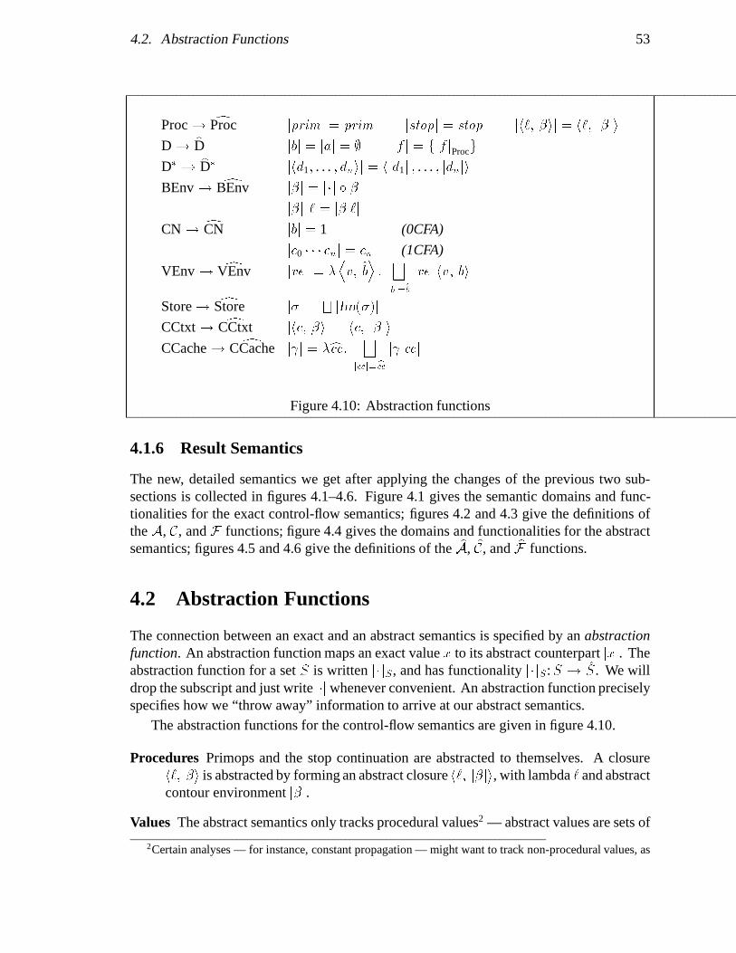
4.2. Abstraction Functions 53
Proc ! dProc jprimj = prim jstopj = stop jh`; �ij = h`; j�ji
D ! bD jbj = jaj = ; jf j = fjf jProcg
D� ! bD� jhd1; . . . ; dnij = hjd1j ; . . . ; jdnji
BEnv ! dBEnv j�j = j�j � �
j�j ` = j� `j
CN ! dCN jbj = 1 (0CFA)
jc0 � � � cnj = cn (1CFA)
VEnv ! dVEnv jvej = �Dv; b
E:G
jbj=b
jve hv; bij
Store ! dStore j�j =FjIm(�)j
CCtxt ! dCCtxt jhc; �ij = hc; j�ji
CCache ! dCCache j j = �ccc:G
jccj=bccj ccj
Figure 4.10: Abstraction functions
4.1.6 Result Semantics
The new, detailed semantics we get after applying the changes of the previous two sub-sections is collected in figures 4.1–4.6. Figure 4.1 gives the semantic domains and func-tionalities for the exact control-flow semantics; figures 4.2 and 4.3 give the definitions ofthe A, C, and F functions; figure 4.4 gives the domains and functionalities for the abstractsemantics; figures 4.5 and 4.6 give the definitions of the bA, bC, and bF functions.
4.2 Abstraction Functions
The connection between an exact and an abstract semantics is specified by an abstractionfunction. An abstraction function maps an exact value x to its abstract counterpart jxj. Theabstraction function for a set S is written j�jS , and has functionality j�jS:S ! S. We willdrop the subscript and just write j�j whenever convenient. An abstraction function preciselyspecifies how we “throw away” information to arrive at our abstract semantics.
The abstraction functions for the control-flow semantics are given in figure 4.10.
Procedures Primops and the stop continuation are abstracted to themselves. A closureh`; �i is abstracted by forming an abstract closure h`; j�ji, with lambda ` and abstractcontour environment j�j.
Values The abstract semantics only tracks procedural values2 — abstract values are sets of
2Certain analyses — for instance, constant propagation — might want to track non-procedural values, as

54 Chapter 4. Control Flow II: Detailed Semantics
abstract procedures from dProc. So booleans and addresses, which obviously are notprocedures, abstract to the empty set: jbj = jaj = ;. A procedure f abstracts to thesingleton set containing its abstract counterpart: fjf jProcg.
Argument Vectors An argument vector of values is simply abstracted elementwise:jhd1; . . . ; dnij = hjd1j ; . . . ; jdnji.
Contour Environments An exact contour environment � is abstracted by composing itwith the contour abstraction function.
Contours The contour abstraction is the critical one that determines most of the otherabstractions.
0CFA In the 0CFA analysis (section 3.6), the abstract semantics has only one abstractcontour, 1. So the 0CFA abstraction is trivial: all contours abstract to 1.
In 0CFA, the exact contour set can simply be taken to be integers, CN = Z; andthe contour allocation function just increments the current contour: nb b c =b+ 1. Note that nb ignores its extra argument c — this is because the eventualabstraction doesn’t need any information at all, so we don’t need to build it into the exact contour. The initial “seed” contour b0 is 0. The abstract contour setis the unity set: dCN = f1g. The contour allocation function always returns 1:cnb b c = 1. The abstraction function abstracts all contours to 1: jbj = 1.
If we use these definitions for CN, b0, nb, dCN, cnb, and j� jCN in the semanticequations given in figures 4.1–4.6, we get a 0CFA interpretation.
1CFA The 1CFA contour abstraction requires a little more machinery. The abstractcontour allocated when entering a lambda is the call site from which the lambdawas called. We need to have this information present in the exact contour sothat the abstraction function can extract it. A straightforward way to do this isto use call strings for the exact contours. A call string is just the string of callsites through which control has passed during the execution of the program.3
Each time a call is performed, the call site is appended to the end of the callstring. Note that in CPS, calls never return, so the current call string is just atrace of the execution path through the program, continuously growing as theprogram executes. The current call string will suffice as a unique “gensym”for the purposes of the exact semantics, since each time a new call string isconstructed, it is longer than all the previously created call strings and henceunique.
If the current contour b = c0 . . . cn when we enter some lambda is the currentcall string, then the call site we just branched from is clearly cn. So the contourwe want for the 1CFA abstraction is cn. Thus our contour abstraction functionjust picks off the last call site in the call string: jc0 . . . cnj = cn.
well. This would be accomplished by specifying a new abstraction function and abstract value domain bD.3Call strings have been used in other interprocedural analysis work [Harrison 89, Sharir+ 81]. This work
usually uses a more complex structure than the simple CPS variant we need here.

4.2. Abstraction Functions 55
So, in the 1CFA model the set of exact contours is just the set of finite strings ofcall sites: CN = LAB�. The initial call string is the label of the top-level call:b0 = ctop. Exact contours are allocated by tacking the current call site onto theend of the current call string: nb b c = bxc. The abstract contour set is simplycall sites: dCN = LAB. When an abstract contour is allocated, it is just taken tobe the current call site: c
nb b c = c. Using these definitions in the equations offigures 4.1–4.6 will give us a 1CFA interpretation.
It’s easy to change the details of this abstraction to come up with variants ona theme. For example, if we take dCN = LAB � LAB, and define c
nb b c =hb#2; ci, then our abstract contours are the last two calls made during programexecution. This would extend 1CFA along the control dimension to a 2CFAabstraction. Alternatively, when entering a closure we could allocate as contourthe pair of call sites (1) the call from which we just branched to the closure and(2) the call from which we previously branched to the the closure’s lexicallysuperior lambda. This would extend 1CFA along the environment dimensionto a different kind of of 2CFA abstraction. There are many ways to abstract theanalysis — 0CFA and 1CFA are not intended to be the last word on this subject.
CN b0 nb b c dCN cnb b c jbj
0CFA Z 0 b+ 1 f1g 1 1
1CFA LAB� ctop bxc LAB c cn; whereb = c0 . . . cn
Table 4.11: 0CFA and 1CFA Contour Machinery
The details of these two contour abstractions are summarised in table 4.11. Note thatwith either of these choices, our domains, allocation policies, and abstractions obeythe following properties:
� nb functions as a gensym.As discussed earlier (section 4.1.1), in order for the exact semantics to be correct,the exact contour set needs to be a partially ordered, and the allocation functionnb must be an increasing function. This is also necessary to guarantee thatthe exact call cache produced by the exact control-flow semantics is a partialfunction (lemma 5).
In 0CFA, the partial order is just arithmetic�; in 1CFA, b � b0 if call string b isa prefix of call string b0. The nb function is clearly increasing for each of thesecontour definitions.
� Contour allocation is homomorphic under abstraction: jnb b xj = cnb jbj jxj.This ensures that the evolution of the abstract interpretation stays linked to theexact interpretation – as successive contours are allocated in the two interpre-
56 Chapter 4. Control Flow II: Detailed Semantics
tations, they stay related due to this property. The proofs that the abstractsemantics safely approximates the exact semantics (section 4.4) rely upon this.In the particular contour allocation machinery we are using, x is a call label c.If we define jcj = c, then both the 0CFA and 1CFA nb functions given abovehave this property:
0CFA: jnb b cj = jb+ 1j = 1 = cnb jbj jcj
1CFA: jnb b cj = jbxcj = c = cnb jbj c = c
nb jbj jcj
� dCN is finite.The computability of the abstract semantics relies upon the finiteness of thecontour set (section 4.4.3).
These are the only properties we require of our contour machinery, so the proofs infollowing sections go through in both the 0CFA and 1CFA cases.
Variable Environments An abstract variable environment maps a variable/abstract-con-tour pair
Dv; b
Eto an abstract value. When an abstracted variable environment
jvej is applied to such a pair, it performs the lookup in the exact environmentve for each variable/exact-contour pair that could abstract to
Dv; b
E. This pro-
duces all the exact values that the corresponding exact lookup might have produced:nve hv; bi
��� jbj = bo
. Each value in this set is then converted to an abstract value, and
all these abstract values are joined together4 to form the result valueFjbj=b
jve hv; bij.
This abstraction is a specific example of a general technique for abstracting functionswhose domains and ranges have abstractions: jf j = �x:
Fjxj=x jf xj. Note that when
f is a partial function (as in the variable environment case), it is assumed that the joinoperation’s index variable x ranges over Dom(f).
Stores In the single-address abstraction introduced in section 3.8.1, an abstract store is justthe set of all values placed into the store. So an exact store abstracts to its contents:j�j =
Fnjdj
��� d 2 Im(�)o=FjIm(�)j.
Call Contexts A call context cc = hc; �i is abstracted by abstracting its component contourenvironment: jccj = hc; j�ji.
Call Caches Call caches are abstracted following the same pattern for variable environ-ments. When the abstracted call cache j j is applied to a call context
Dc; b�
E, we apply
the exact call cache to all the exact call contexts that could abstract toDc; b�
E. All
the result procedures are abstracted and joined together5 to produce the result value:j j
Dc; b�
E=Fjccj=hc; b�i j ccj =
Fj�j=b� j hc; �ij.
4Since abstract values are sets of abstract procedures, and the join operation for bD is set union, this justmeans all the abstract procedures are collected together into one set.
5That is, collected into a set.

4.3. Existence 57
4.3 Existence
In the exact semantics, the only values whose existence is non-obvious are the C and Ffunctions. The value sets, such as D, Proc, and VEnv, and the semantic functionsPR andA are all defined with simple, constructive definitions, and clearly exist. C and F , on theother hand, are defined with recursive equations, and so we must go to a little trouble toprove these equations are well-defined and admit a solution.
We will define C and F as the least fixed point of a functional H . That is, we’ll definea series of approximations C0; C1; . . . and F0;F1; . . . to C and F , such that hCi+1; Fi+1i =H hCi; Fii. If we can show that H is a continuous operator, then it has a least fixed point,which will be the limit of our approximation series:
hC; Fi = H hC; Fi =Gi�0
hCi; Fii:
This is the standard method of constructing functions from recursive definitions in denota-tional semantics.
We take the definition of H from the recursive definitions of C and F given in figures4.2 and 4.3. hC 00; F 00i = H hC0; F 0i is just the value we get if we define hC 00; F 00i from thefigure 4.2 and 4.3 definitions, using the functions C 0 and F 0 for the recursive calls insidethe equations. Clearly, we are seeking a solution to the equation hC; Fi = H hC; Fi.
4.3.1 H is well-defined
First, we need to determine that H is a well-defined functional. This is guaranteed for usby the constraints we placed on values from CState and FState. Suppose we apply H to apair hC 0; F 0i, getting result hC 00; F 00i.
Consider C 00 first. Suppose C 00 is being applied to an argument tuple hc; �; ve ; b; �i. Ifthe call expression c is a simple call [[(f a1 . . .an)]], then C 00 uses the partial function A toevaluate the procedure f and arguments ai. The C-ENVa constraint (Figure 4.7) on c, �,and ve guarantee that the arguments passed toA are all within the partial function’s domain.So all evaluations with A are well-defined within C 00. We also need to show that in therecursive call toF 0, the arguments that C 00 passes (f 0, av , ve , b, and �) satisfy the constraintsof FState so that the application is correct. C 00 does not alter the variable environment orstore, so to show the environment constraint F-ENV, we need only show that the proceduref 0 and arguments av are all consistent with ve . If the procedure expression f or an argumentai is a constant or primop, A will certainly evaluate it to a non-closure, so we can ignoreit. If it is a variable, A will evaluate it to some already-existing value in Im(ve), so theconstraints on C 00 guarantee us the value is consistent with ve . On the other hand, if theexpression is a lambda `, then A will evaluate it to a new closure h`; �i; we need to showthat this new closure is consistent with the variable environment. This is straightforward.Suppose lambda ` is an argument of call c, and is being closed in environment �=ve . TheCState constraint requires Dom(�) to include c’s lexical context, that is, every lambdalexically superior to c. This is `’s lexical context as well, so the F-ENVa half of the FState
58 Chapter 4. Control Flow II: Detailed Semantics
environment constraint is satisfied. The CState constraint C-ENVa also requires ve tocover �, so the F-ENVb half of FState’s environment constraint is satisfied as well. We’vesyntactically restricted primop applications to be of correct arity, so the F-ARITY constraintis preserved if c happens to be a primop application. Clearly, since C 00 does not allocateany new addresses or alter the store, the address constraint F-ADDR is preserved in thearguments it passes to F 0. So C 00 is well-defined in the simple-call case.
Suppose that the call expression c that C 00 is evaluating is instead a letrec expression:[[(letrec ((f1 l1). . .) c0)]]. In this case, C 00 recursively calls C 0 to evaluate the internalcall expression in an augmented environment �0=ve 0. To show that this application ofC0 is well-defined, we need to verify that it is applied to arguments satisfying the CStateconstraints. Again, clearly the store constraint C-ADDR is preserved, since the store isunchanged, and no new addresses are introduced into the system. Verifying the environmentconstraint C-ENV means showing that the inner call expression c0 is consistent with theenvironment structure that C 00 builds, and showing that each closure hli; �0i created by theletrec is consistent with the updated variable environment ve 0.
To show that a letrec closure hli; �0i is consistent with ve 0, we need to show first thatthe domain of �0 contains li’s lexical context. li’s lexical context is the lexical context ofc plus the binding introduced by the letrec itself. This is just Dom(�) [ fcg, which isprecisely the domain of �0. Similarly, ve 0 covers � 0 by construction. The new variableenvironment ve 0 is the old ve plus an update
�hfi; b
0i 7! A li �0 ve
�, where b0 = nb b. If a
binding construct `0 is in the domain of � 0 = ��c 7! b0
�, then either it is c or it is in Dom(�).
If it is the letrec c, then the update portion of ve 0 (i.e.,�hfi; b
0i 7! A li �0 ve
�) handles all
of the letrec’s variables. If it is in Dom(�), then the old portion of ve 0 (i.e., ve ) handlesall of the variables bound by `0.
Showing that F 00 is well-defined follows similar reasoning. When F 00 is applied to aclosure h`; �i, we need to show that the internal application of C 0 has arguments satisfyingthe CState constraints. This is straightforward. We know that the arguments of F 00 satisfythe FState constraints. This means that h`; �i is consistent with the variable environment ve(by F-ENV). After augmenting the environment structure to bind the lambda `’s variables,the resulting environment must be consistent with the lambda’s internal call expression.Since the store remains unaltered, its constraints remain satisfied. No new addresses orclosures are added to the system, so the other constraints remain satisfied.
The primop cases in the definition of F 00 generally involve recursive applications ofF 0 to invoke the primop continuation. So we need to show that the arguments used in therecursive applications satisfy the FState constraints. Consider the addition operator. Nonew environment contexts or addresses are introduced into the system, and the continuation,being a first-class value, can’t be a primop, so the constraints are all trivially satisfied. Theif, contents, and set primops are similar. The new primop, however, does introduce anew address into the system. Since this address is defined by the result store passed alongto the recursive F 0 application, however, we continue to satisfy the FState constraints.
4.3. Existence 59
4.3.2 H is continuous
Now that we’ve established H is a well-defined operator, we need to show that it is acontinuous one, which will allow us to take its fixed point. Continuous operators operateon values taken from a cpo. H operates on values taken from the space
(CState ! CCache)� (FState ! CCache):
This space is a cpo, under the pointwise ordering induced by the ordering on call caches.Call caches are ordered by set inclusion: v 0 iff � 0. So the cpo upon which H actshas bottom value ? = h�cs: ;; �fs: ;i.
H is a continuous operator if
� it preserves chains:h hCi; Fii j i � 0 i a chain ) hH hCi; Fii j i � 0 i a chain
� it preserves limits on chains:H
Fi�0
hCi; Fii =Fi�0
H hCi; Fii.
Lemma 1 H is monotonic
This follows straightforwardly from the form of H .
Lemma 2 H preserves limits on chains. That is, if h hCi; Fii j i � 0 i is a chain, thenH
Fi�0 hCi; Fii =
Fi�0 H hCi; Fii.
Proof: Let hC1; F1i be the limit of the chain: hC1; F1i =F
i�0 hCi; Fii. Let hC 0; F 0i =H hC1; F1i and hC 00; F 00i =
Fi�0 H hCi; Fii. We want to show that hC 0; F 0i = hC 00; F 00i.
Part 1: C 0 = C 00
Let cs be some argument drawn from CState — that is, cs is a tuple hc; �; ve ; b; �i.The call expression c is either a simple call or a letrec. Suppose it is a simple call,and that evaluation of the call doesn’t cause an immediate run-time error. Then
C0 cs = fhcc; fig [ F1 fs;
where cc = hc; �i and F1 fs is the recursive call to F1, with fs the appropriateargument tuple. On the other hand,
C00 cs =[i
�fhcc; f ig [ Fi fs
�
= fhcc; fig [[i
Fi fs
= fhcc; fig [ F1 fs:
So C 0 cs = C00 cs .

60 Chapter 4. Control Flow II: Detailed Semantics
If evaluation of the call’s subforms causes a run-time error, then the situation is evensimpler, since all the functions abort and produce the empty cache:
C00 cs =[i
; = ; = C0 cs :
If c is not a simple call, then it is a letrec expression: [[(letrec ((f1 l1). . .) c0)]].In this case,
C0 cs = C1 cs 0;
where cs 0 is the argument value passed on the recursive call to evaluate the letrec’sinner call expression c0. However,
C00 cs =[i
Ci cs0 = C1 cs 0:
So C 0 cs = C00 cs .
In either case, C 0 cs = C00 cs , and so C 0 = C00.
Part 2: F 0 = F 00
The main recursive case proceeds along the same lines as its C 0 = C00 counterpart. Letfs be some argument drawn from FState — that is, fs is a tuple hf; av ; ve ; b; �i. Sup-pose that the procedure f is a closure, and that processing the procedure applicationdoesn’t cause a run-time error.
F 0 fs = C1 cs ;
where cs the appropriate argument tuple for the recursive call to C1. On the otherhand,
F 00 fs =[i
Ci cs = C1 cs :
So F 0 fs = F 00 fs .
Suppose instead that the procedure f is a primop, and, again, that no run-time errorsare caused. We’ll only consider the f = [[p:+]] case here; the others primops aresimilar. In this case,
F 0 fs =nDD
icp:+; bE; kEo
[ F1 fs 0;
wherenDD
icp:+; bE; kEo
records the immediate call to the continuation, and F1 fs 0
is the recursive application that actually handles the continuation. Considering F 00,we have
F 00 fs =[i
�nDDicp:+; b
E; kEo
[ Fi fs0�=nDD
icp:+; bE; kEo
[ F1 fs 0:
So F 0 fs = F 00 fs .
If f = stop or fs causes a run-time error, then, just as in the C error case, both F 0 andF 00 trivially return the empty call cache ;.
In either event, F 0 fs = F 00 fs . So F 0 = F 00.

4.4. Properties of the Semantic Functions 61
Q.E.D.
Theorem 3 H is continuous
Proof: This follows from the two previous lemmas.
Corollary 4 H has a least fixed point: hC; Fi = fix H .
Proof: Continuous functions have least fixed points.This suffices to show the main result of this section: the C and F functions exist. We
also need to know that the abstract functions bC and bF exist. This involves showing thattheir defining functional cH is well-defined and continuous. I omit the actual proof of thisfact, as it is almost identical to the proof for C and F .
4.4 Properties of the Semantic Functions
Now that we know C, F , A, PR and their abstract counterparts exist, we can proceed toproving properties about them. In this section we’ll work out proofs to show
� The answer returned by PR is actually a partial function.
� dPR safely approximates PR.
� dPR is computable.
The proof technique we’ll use to show most of these theorems and their supporting lemmasis the technique of fixed-point induction.
Suppose that � is a predicate on some cpo D. � is an admissible predicate if � holdsover a chain h di j i � 0 i implies that � holds on the limit: � h di j i � 0 i ) �
Fi di: It
is a simple theorem that if � is an admissible predicate on D, H:D ! D is a continuousfunction, �?, and � d) � (H d), then � (fix f). This is a standard proof technique foundin most introductory texts on denotational semantics [Brookes 89, Schmidt 86, Stoy 77].
4.4.1 Call caches are partial functions
Lemma 5 The call cache returned by C or F is always a partial function.
Informal proof: Each timeF calls C, it passes along a new contour environment � that hasnever been created before. The contour environment is guaranteed to be unique becausethe innermost contour was newly allocated by F . So C’s update hhc; �i; f 0i is guaranteedunique in �. Similar reasoning applies to the cache entries made by the primops: theircache entries always have a contour environment containing a newly allocated contour, sothe environment is guaranteed unique. No collisions among the entries means the resultcache is a partial function.

62 Chapter 4. Control Flow II: Detailed Semantics
A careful proof would use an admissible predicate formalising the above ar-gument. The predicate would be something like: if C’s argument has (1) bdominating all contours in the system, and (2) � does not occur in the systemthen (3) the returned call cache is a partial function and (4) b lower boundsthe innermost contour of every entry in the returned call cache . . . with similarstatements about F .
Establishing that our semantic functions produce partial functions allows us to do twouseful things. First, we can now manipulate the result call cache in functional ways e.g.,we can apply it to values: cc . Second, we can take the call cache updates in the definingequations to be either a set update ( [ fhhc; �i; f ig) or a function update (
�hc; �i 7! f
�)
as convenient, since the result is the same.
4.4.2 Abstract semantics is a safe approximation
In this section, we will show that our abstract control-flow analysis gives a safe approxi-mation to the exact analysis.
First, we need to define formally what we mean by “conservatively approximates.” Anexact call-cache can have an infinite domain and image — it is a table that gives infinitelyprecise answers to infinitely precise queries. At compile time, however, we are restrictedto asking finitely precise queries, and receiving finitely precise answers. Thus, an abstractcall-cache has finite domain and range.
Now, an abstract call context ccc 2 dCCtxt corresponds to a set of exact call contexts,that is, the set of all exact call contexts that abstract to ccc:
ncc
��� jccj = ccco:
That is, the finitely precise abstract call context ccc describes a set of potential exact callcontexts.
Similarly, an abstract procedure f 2 bD corresponds to a set of exact procedures, that is,the set of all exact procedures that abstract to values contained in f :
nf��� jf j v f
o:
(In this case jf j = fjf jProcg, so jf j v f means jf jProc 2 f .)
So, when we query an abstract call cache with some abstract call context ccc, we getback an abstract procedure ccc that describes a set of exact procedures:
nf��� jf j v ccc
o:
If we query an exact call cache with the equivalent set of exact call contexts, we get
n cc
��� jccj = ccco:
4.4. Properties of the Semantic Functions 63
Our abstract call cache is a safe approximation if the approximate answer to our approximatequery ccc contains the exact answer to our approximate query:
n cc
��� jccj = ccc o � nf��� jf j v ccc o :
The left-hand side is the set of all procedures that were really called from some call contextdescribed by the abstraction ccc . The inclusion guarantees us that all of these proceduresare included in the answer the abstract call cache produces. This inclusion is equivalent tostating that
jccj = ccc ) j ccj v ccc:So, stating that “ conservatively approximates ” can be formally stated as “j ccj v jccj :” We can extend this concept to any exact/abstract pair of functions:
Definition 3
f conservatively approximates (c.a.) f if f jxj w jf xj (i.e., f � j�j w j�j �f ).
f strongly conservatively approximates (s.c.a.) f if x w jxj ) f x w jf xj.
If f is a partial function, it is understood that x is restricted to Dom(f ) in theabove comparisons.
“Strongly conservatively approximates,” is an even stronger condition than simple “con-servatively approximates,” and will be of use in our upcoming proofs of correctness.
Note the extra qualification in this definition for the partial function case. We glossedover this detail in the above discussion: , a partial function, is not defined over all thecc to which we might apply it in the expression
n cc
��� jccj = ccc o : When cc =2 Dom( ),then there is no call recorded in the cache for that call context, so the correct expressionisn cc
��� jccj = ccc ^ cc 2 Dom(cc)o: With this qualification, our definition correctly
expresses the notion of safe approximation in the partial function case as well as the totalfunction one.
In this section we will prove as lemmas that (roughly speaking) bA, bC, and bF conserva-tively approximate A, C, and F , respectively. With these lemmas, we can show the mainresult of this section:
Theorem 6 dPR ` conservatively approximates PR `.That is, � j�j w j�j � , where = dPR `, = PR `.
Proof: The theorem follows from the fact that bF conservatively approximates F .Let = PR ` and = dPR `.
= dPR ` = bF hh`; [ ]i; hfstopgi; [ ]; jb0j; [ ]i t�hctop; [ ]i 7! fh`; [ ]ig
� = dPR ` = F hh`; [ ]i; hstopi; [ ]; b0; [ ]i
�hctop; [ ]i 7! h`; [ ]i
�
There are two cases to consider.

64 Chapter 4. Control Flow II: Detailed Semantics
� cc = hctop; [ ]i:
jccj = jhctop; [ ]ij = hctop; [ ]i w fh`; [ ]ig ;
j ccj = j hctop; [ ]ij = jh`; [ ]ij = fh`; [ ]ig :
So, jccj w j ccj.
� cc 6= hctop; [ ]i:
jccj = bF hh`; [ ]i; hfstopgi; [ ]; jb0j; [ ]i jccj
j ccj = jF hh`; [ ]i; hstopi; [ ]; b0; [ ]i ccj
Now, jh`; [ ]ij = h`; [ ]i, jhstopij = hfstopgi, and j[ ]j = [ ], so
jccj w j ccj
by the conservative approximation property of F and bF (lemma 9).
In either case, jccj w j ccj, and the theorem is shown. Q.E.D.Now, let’s prove the supporting lemmas of the above theorem. Because bA and A are
defined non-recursively, the proof of their approximation lemma is correspondingly direct.
Lemma 7 bA acve j�j w jA a ve �j where cve w jvej. (s.c.a. in ve and c.a. in �.)
Proof by cases:
1. a = [[k]] or a = [[prim]] (constant or primop)Immediate.
2. a = [[`:(� (v1 . . . vn) c)]] (lambda)
bA ` ve j�j = fh`; j�jig
jA ` ve �j = jh`; �ij = fh`; j�jig
3. a = [[r:v]] (variable reference)Let ` = binder v.
bA r cve j�j = cve hv; j�j `i w jve j hv; j�j `i
=G
jbj=j�j `
jve hv; bij w jve hv; � `ij
= jA r ve �j
Q.E.D.The next two lemmas use the elementwise ordering on dCState and dFState. Note that the c,b�, and b components of a dCState tuple, and the f , b components of a dFState tuple are ordered
discretely. This means, for example, that ifDc1;
b�1; cve 1; b1; b�1
EvDc2;
b�2; cve2; b2; b�2
E,
it must be the case that c1 = c2, b�1 = b�2, and b1 = b2.

4.4. Properties of the Semantic Functions 65
Lemma 8 bC bcs jccj w jC cs ccj, where bcs w jcsj. (s.c.a. in cs, and c.a. in cc)Equivalently: Suppose cs = hc; �; ve; b; �i 2 CState and bcs = hc; j�j; cve; jbj; b�i 2dCState such that bcs w jcsj. Let = C hc; �; ve; b; �i and = bC hc; j�j; cve; jbj; b�i. Thencc 2 Dom( ) ) jccj w j ccj.
Lemma 9 bF bfs jccj w jF fs ccj, where bfs w jfsj. (s.c.a. in fs, and c.a. in cc)Equivalently: Suppose fs = hf; av; ve; b; �i 2 FState and bfs = hjf j; cav; cve; jbj; b�i 2dFState such that bfs w jfsj. Let = F hf; av; ve; b; �i and = bF hjf j; cav; cve; jbj; b�i.Then cc 2 Dom( ) ) jccj w j ccj.
The “equivalent” restatements of these lemmas take advantage of the observation that w j j iff c.a. . This is due to the definition of j�jCCache (figure 4.10).
Proofs of the Inductive Case
Because of their recursive definitions, the approximation lemmas for C, bC, F and bF areproved with a fixed-point induction. The following proofs will proceed in two distinctsteps. First, we’ll “prove” the lemmas in a recursive fashion: the proofs of the lemmas willactually assume the lemmas already hold for the applications of the semantic functions inthe recursive expansions of the function definitions. This does not constitute a sound proof.These “recursive proofs” do, however, establish the inductive case of the related admissiblepredicate. This is the part of the proof that provides the most insight, and so we’ll handleit separately. The extra issues of showing the base case and the limit case are uninterestingmachinery, and will be addressed in the following text.
As we discussed in section 4.2, our contour abstraction and allocation functions arerelated by the identity jnb b cj = cnb jbj c. We’ll be using these two expressions inter-changeably in the proofs of the following two lemmas.
Lemma 8 Proof of Inductive Case ( bC conservatively approximates C)Recursion assumption: C and bC are defined in terms of C and bC functions for which lemma8 holds, and F and bF functions for which lemma 9 holds.
Suppose the call expression being evaluated is a simple call, [[c:(f a1 . . . an)]]. Letf = bA f j�j cve , cav#i = bA ai j�j cve , and f 0 = A f � ve . If f 0 =2 Proc, then C encounters arun-time error, and aborts with the empty cache [ ]. In this case, the lemma holds trivially.Suppose, instead, that f 0 2 Proc.
bC hc; j�j; cve; jbj; b�i=hhc; j�ji 7! f
itGf 02f
bF Df 0; cav ; cve; cnb jbj c; b�E (4.1a)
w�hc; j�ji 7! jf 0j
�t
Gf 02jf 0j
bFDf 0; cav ; cve ; cnb jbj c; b�
E(4.1b)
=�hc; j�ji 7! jf 0j
�t bF D
jf 0jProc; cav ; cve; cnb jbj c; b�E (4.1c)
66 Chapter 4. Control Flow II: Detailed Semantics
Equation 4.1a is the definition of bC. Equation 4.1b holds because bA approximatesA (lemma7), so that jf 0j v f . The join over f 0 2 jf 0j can be discarded, because jf 0j = fjf 0jProcg is asingleton set, giving us equation 4.1c.
a. cc = hc; �i
bC hc; j�j; cve ; jbj; b�i jccjw��hc; j�ji 7! jf 0j
�t bF D
jf 0jProc; cav ; cve ; cnb jbj c; b�E� hc; j�ji (by 4.1)
w jf 0j
jC hc; �; ve ; b; �i ccj
= j�F hf 0; av ; ve ; nb b c; �i
� �hc; �i 7! f 0
�hc; �ij = jf 0j (by def’n C)
Therefore, bC hc; j�j; cve ; jbj; b�i jccj w jC hc; �; ve ; b; �i ccj.
b. cc 6= hc; �i
bC hc; j�j; cve ; jbj; b�i jccjw��hc; j�ji 7! jf 0j
�t bF D
jf 0jProc; cav ; cve ; cnb jbj c; b�E� jccj (by 4.1)
= bF Djf 0jProc; cav ; cve ; cnb jbj c; b�E jccj
= bF hjf 0jProc; cav ; cve ; jnb b cj; b�i jccj
jC hc; �; ve ; b; �i ccj = j�F hf 0; av ; ve; nb b c; �i
� �hc; �i 7! f 0
�ccj
= jF hf 0; av ; ve; nb b c; �i ccj
Therefore, bC hc; j�j; cve ; jbj; b�i jccj w jC hc; �; ve ; b; �i ccj by c.a. on F .
Suppose, instead, that C is evaluating a letrec form, [[c:(letrec ((f1 l1). . .) c0)]].Let b0 = nb b c (so that jb0j = cnb jbj c), and �0 = �
�c 7! b0
�(so that j�0j = j�j
�c 7! jb0j
�).
bC hc; j�j; cve ; jbj; b�i jccj = bCDc0; j�0j; cve t
hhfi; jb
0ji 7! bA li j�0j cve
i; jb0j; b�
Ejccj
jC hc; �; ve; b; �i ccj = jC hc0; �0; ve�hfi; b
0i 7! A li �0 ve
�; b0; �i ccj
The result follows from (1) cve t hhfi; jb
0ji 7! bA li j�0j cvei w jve
�hfi; b
0i 7! A li �0 ve
�j
(shown below), and (2) the recursion assumption on C and bC.To see that
cve t hhfi; jb0ji 7! bA li j�0j cvei w jve
�hfi; b
0i 7! A li �0 ve
�j ;
let g be the expression on the left, and h be the expression on the right.

4.4. Properties of the Semantic Functions 67
g hfi; jb0ji w h hfi; jb
0ji
g hfi; jb0ji = bA li j�
0j cve t cve hfi; jb0ji w bA li j�0j cve t jve j hfi; jb0ji
= bA li j�0j cve t G
jb00j=jb0j
jve hfi; b00ij
w bA li j�0j cve t G
jb00j=jb0j
b00 6=b0
jve hfi; b00ij
w jA li �0 ve j t
Gjb00j=jb0j
b00 6=b0
jve hfi; b00ij
h hfi; jb0ji =
Gjb00j=jb0j
jve�hfi; b
0i 7! A li �0 ve
�hfi; b
00ij
= jA li �0 ve j t
Gjb00j=jb0j
b00 6=b0
jve hfi; b00ij
gDv; b
Ew h
Dv; b
Efor
Dv; b
E6= hfi; jb
0ji
gDv; b
E= cve D
v; bE
hDv; b
E=
Gjb00j=b
jve�hfi; b
0i 7! A li �0 ve
�hv; b00ij
=G
jb00j=b
jve hv; b00ij = jve jDv; b
E
The hv; b00i lookup skips past the�hfi; b
0i 7! A li �0 ve
�environment update because
either v 6= fi or b 6= jb0j. In the first case, the lookup obviously skips the update. Inthe second case, jb00j = b, so jb00j 6= jb0j, and therefore b00 6= b0 — also causing thelookup to skip the update.
This completes the recursive proof that bC conservatively approximates C.Q.E.D.
Lemma 9 Proof of Inductive Case ( bF conservatively approximates F)Recursion assumption: F and bF are defined in terms of C and bC functions for which lemma8 holds, and F and bF functions for which lemma 9 holds.
The argument f is either a closure, the stop continuation, or a primop. We will showeach case in turn. We may assume for all the cases that none of the run-time error checksapply. Otherwise, F aborts with the empty cache [ ], and the lemma holds trivially.
Assume the procedure is a closure: f = h[[`:(� (v1 . . . vn) c)]]; �i.
F hh`; �i; av ; ve ; b; �i cc = C hc; ��` 7! b
�; ve
�hvi; bi 7! av#i
�; b; �i cc
bF hh`; j�ji; cav ; cve; jbj; b�i jccj = bC hc; j�j �` 7! jbj�; cve t �hvi; jbji 7! cav#i�; jbj; b�i jccj
68 Chapter 4. Control Flow II: Detailed Semantics
The result follows from (1) j��` 7! b
�j = j�j
�` 7! jbj
�, (2) cve t �
hvi; jbji 7! cav#i� wjve
�hvi; bi 7! av#i
�j (shown below), and (3) the recursion assumption on C and bC.
To see thatcve t �hvi; jbji 7! cav#i� w jve
�hvi; bi 7! av#i
�j ;
let g be the expression on the left, and h be the expression on the right.
a. g hvi; jbji w h hvi; jbji
g hvi; jbji = cav#i t cve hvi; jbji w jav#ij t jvej hvi; jbji
= jav#ij tG
jb0j=jbj
jve hvi; b0ij w jav#ij t
Gjb0j=jbj
b0 6=b
jve hvi; b0ij
h hvi; jbji =G
jb0j=jbj
jve�hvi; bi 7! av#i
�hvi; b
0ij = jav#ij tG
jb0j=jbj
b0 6=b
jve hvi; b0ij
Therefore, g hvi; jbji w h hvi; jbji.
b. gDv; b
Ew h
Dv; b
Efor
Dv; b
E6= hvi; jbji
gDv; b
E= (cve t �hvi; jbji 7! cav#i�) Dv; bE = cve D
v; bEw jvej
Dv; b
E
hDv; b
E=
Gjb0j=b
jve�hvi; bi 7! av#i
�hv; b0ij =
Gjb0j=b
jve hv; b0ij = jvejDv; b
E
Therefore, gDv; b
Ew h
Dv; b
E.
Alternatively, the procedure could be the stop continuation. This is a trivial case, sinceF produces the empty call cache which abstracts to the empty abstract call cache that bFreturns.
Finally, the procedure could be one of the primops: +, if, new, contents, and set.Suppose that f = [[p:+]]. Let
= bF D[[p:+]];
Dx; y; k
E; cve ; jbj; b�E
=hDicp:+; j�j
E7! k
itGk02k
bF Dk0; h?i; cve; cnb jbj icp:+; b�
E
whDicp:+; j�j
E7! jkj
it
Gk02jkj
bF Dk0; h?i; cve ; cnb jbj icp:+; b�
E
=hDicp:+; j�j
E7! jkj
it bF D
jkjProc; h?i; cve;���nb b icp:+
���; b�E
= F h[[p:+]]; hx; y; ki; ve ; b; �i
= (FDk; hx+ yi; ve; nb b icp:+; �
E)hDicp:+; �
E7! k
i;
where � =�[[p:+]] 7! b
�, so that j�j =
�[[p:+]] 7! jbj
�. We want to show that jccj w j ccj.
4.4. Properties of the Semantic Functions 69
cc =Dicp:+; �
E
jccj w jkj and j ccj = jkj.
cc 6=Dicp:+; �
E
jccj w bF DjkjProc; h?i; cve ;
���nb b icp:+
���; b�E jccjj ccj =
���FDk; hx+ yi; ve ; nb b icp:+; �
Ecc���
By bF c.a. F , jccj w j ccj.
Showing the lemma for the rest of the primops involves minor variations on the + case.Suppose that f = [[p:if]]. Let
= bF D[[p:if]];
Dx; k0; k1
E; cve ; jbj; b�E
=
0@ G
f2k0
bF Df; hi; cve ; cnb jbj ic0
p:if; b�E1A t
0@ G
f2k1
bF Df; hi; cve; cnb jbj ic1
p:if; b�E1A
thDic0
p:if; j�jE7! k0;
Dic1
p:if; j�jE7! k1
i
w
0@ G
f2jk0j
bF Df; hi; cve ; cnb jbj ic0
p:if; b�E1A t
0@ G
f2jk1j
bF Df; hi; cve; cnb jbj ic1
p:if; b�E1A
thDic0
p:if; j�jE7! jk0j;
Dic1
p:if; j�jE7! jk1j
i
= bF Djk0jProc; hi; cve;
���nb b ic0p:if
���; b�E t bF Djk1jProc; hi; cve ;
���nb b ic1p:if
���; b�E
thDic0
p:if; j�jE7! jk0j;
Dic1
p:if; j�jE7! jk1j
i
= F h[[p:if]]; hx; k0; k1i; ve ; b; �i
= x 6= false �! FDk0; hi; ve ; nb b ic0
p:if; �E hD
ic0p:if; �
E7! k0
i
otherwise FDk1; hi; ve ; nb b ic1
p:if; �E hD
ic1p:if; �
E7! k1
i;
where� =�[[p:if]] 7! b
�, so that j�j =
�[[p:if]] 7! jbj
�. We want to show that jccj w j ccj.
We have to be a little bit careful in manipulating the various subexpressions of the exactcache returned for if. Exact caches are partial functions, and although cc is assumed to liewithin Dom( ), that does not imply that we can apply the caches for both arms of the if tocc — it is possibly in the domain of only one of these arms. The following development iscareful to handle this small complexity.
cc =Dic0
p:if; �E
In this case, we are looking up the call to the true continuation k0.
jccj = Dic0
p:if; j�jEw jk0j t bF D
jk1jProc; hi; cve ;���nb b ic0
p:if
���; b�E jccj

70 Chapter 4. Control Flow II: Detailed Semantics
Suppose that x 6= false. Then j ccj = jk0j, and the conservative inequality holds.Alternatively, suppose that x = false. Then
j ccj =����F D
k1; hi; ve ; nb b ic0p:if; �
E hDic1
p:if; �E7! k1
i�cc���
=���F D
k1; hi; ve ; nb b ic0p:if; �
Ecc��� ;
and the result follows from the recursion assumption on F and bF .
cc =Dic1
p:if; �E
In this case, we are looking up the call to the false continuation k1. This case isanalagous to the previous case for the true continuation.
cc 6=Dic0
p:if; �E;Dic1
p:if; �E
The final case involves looking up some call other than the two immediate potentialcalls to the if primop’s continuations.
jccj w bFDjk0jProc; hi; cve;
���nb b ic0p:if
���; b�Ejccj
t bF Djk1jProc; hi; cve;
���nb b ic1p:if
���; b�E jccjSuppose that x 6= false. Then
j ccj =���F
Dk0; hi; ve; nb b ic0
p:if; �Ecc��� ;
and the result follows from the recursion assumption on F and bF . Alternatively,suppose that x = false. Then
j ccj =���F D
k1; hi; ve; nb b ic1p:if; �
Ecc��� :
Again, the result follows from the recursion assumption on F and bF .
Suppose that f = [[p:new]]. Let
= bF D[[p:new]];
Dd; k
E; cve; jbj; b�E =hD
icp:new; j�jE7! k
itGk02k
bF Dk0; h?i; cve ; cnb jbj icp:new; (b� t d)
E
= F h[[p:new]]; hd; ki; ve ; b; �i =
FDk; hai; ve; nb b icp:new; �
�a 7! d
�E hDicp:new; �
E7! k
i;
where � =�[[p:new]] 7! b
�(so that j�j =
�[[p:new]] 7! jbj
�) and a = alloc �. We want to
show that jccj w j ccj.
cc =Dicp:new; �
E
jccj w k w jkj and���h cc
��� = jkj.
4.4. Properties of the Semantic Functions 71
cc 6=Dicp:new; �
E
jccj wGk02k
bF Dk0; h?i; cve ; cnb jbj icp:new; (b� t d)
Ejccj
w bFDjkjProc; h?i; cve;
���nb b icp:new
���; (b� t d)Ejccj
j ccj =���F D
k; hai; ve; nb b icp:new; ��a 7! d
�Ecc���
The result follows from bF c.a. F and b� t d w j��a 7! d
�j.
To see that b� t d w j��a 7! d
�j:
j��a 7! d
�j =
GjIm(�
�a 7! d
�)j v
GjIm(�) [ fdgj
=GjIm(�)j t jdj = j�j t jdj v b� t d
Suppose that f = [[p:set]]. Let
= bF D[[p:set]];
Da; d; k
E; cve; jbj; b�E =hD
icp:set; j�jE7! k
itGk02k
bF Dk0; hi; cve ; cnb jbj icp:set; (b� t d)
E
= F h[[p:set]]; ha; d; ki; ve; b; �i =
(FDk; hi; ve; nb b icp:set; �
�a 7! d
�E)hDicp:set; �
E7! k
i
where � =�[[p:set]] 7! b
�, so that j�j =
�[[p:set]] 7! jbj
�. We want to show that jccj w
j ccj.
cc =Dicp:set; �
E
jccj w k w jkj and j ccj = jkj.
cc 6=Dicp:set; �
E
jccj wGk02k
bF Dk0; hi; cve ;
���nb b icp:set
���; (b� t d)Ejccj
w bF DjkjProc; hi; cve;
���nb b icp:set
���; (b� t d)Ejccj
j ccj =���F D
k; hi; ve; nb b icp:set; ��a 7! d
�Ecc���
The result follows from bF c.a. F and (as in the case of new) b� t d w j��a 7! d
�j.
Suppose that f = [[p:contents]]. Let
= bF D[[p:contents]];
Da; k
E; cve ; jbj; b�E =hD
icp:contents; j�jE7! k
itGk02k
bF Dk0; hb�i; cve; cnb jbj icp:contents; b�
E
72 Chapter 4. Control Flow II: Detailed Semantics
= F h[[p:contents]]; ha; ki; ve ; b; �i =
(FDk; h� ai; ve; nb b icp:contents; �
E)hDicp:contents; �
E7! k
i;
where � =�[[p:contents]] 7! b
�, so that j�j =
�[[p:contents]] 7! jbj
�. We want to show
that jccj w j ccj.
cc =Dicp:contents; �
E
jccj w k w jkj and j ccj = jkj.
cc 6=Dicp:contents; �
E
jccj wGk02k
bF Dk0; hb�i; cve ;
���nb b icp:contents
���; b�E jccj
wG
k02jkj
bF Dk0; hb�i; cve ;
���nb b icp:contents
���; b�E jccj
= bFDjkjProc; hb�i; cve;
���nb b icp:contents
���; b�Ejccj
j ccj =���F D
k; h� ai; ve; nb b icp:contents; �Ecc���
j� aj v j�j v b�, and the result follows from bF c.a. F .
This completes the recursive proof that bF conservatively approximates F .Q.E.D.
Proofs of the Base and Limit Cases
Recall from section 4.3 that the C and F functions are defined as the limit of a sequenceof approximations h hCi; Fii j i � 0 i generated by the H functional, such that hCi; Fii =
H i ?. Similarly, bC and bF are the limit of an approximation sequenceD D bCi; bFi
Ej i � 0
E,
generated by some cH functional. We prove properties of C, F , bC, and bF with the techniqueof inductive predicates. With this technique, a complete proof of the two previous lemmasinvolves showing the lemma holds in three cases:
� The base case.That is, showing that the lemmas hold on
DC0; F0; bC0; bF0
E.
� The inductive case.That is, showing that if the lemmas hold on
DCi; Fi; bCi; bFi
E, then they hold onD
Ci+1; Fi+1; bCi+1; bFi+1
E.
� The limit case.That is, showing that if the lemmas hold over a chain
D DCi; Fi; bCi; bFi
Ej i � 0
E,
then they hold on the limit of the chainFi�0
DCi; Fi; bCi; bFi
E.
The recursive proofs we’ve just completed establish the inductive case. We still need toshow the lemmas hold in the base and limit cases.
4.4. Properties of the Semantic Functions 73
Proof of Base CaseOur quadruples of functions
DCi; Fi;
bCi; bFi
Eare taken from the cpo
(CState ! CCache)� (FState ! CCache)� ( dCState ! dCCache)� ( dFState ! dCCache):
The ordering on this cpo is pointwise over each element of the quadruple. So the bottomelement of the cpo is
DC0; F0;
bC0;bF0
E=D�cs : [ ]; �fs : [ ]; �ccs : [ ]; � bfs : [ ]
E;
where the exact empty call caches from CCache are empty partial functions (i.e., [ ] = ;),and the approximate empty call caches from dCCache are total functions mapping all inputsto the empty set (i.e., [ ] = �cc: ;).
To establish the base case for lemmas 8 and 9, we must show they hold for the bottomtuple of functions
DC0; F0; bC0; bF0
E. This is trivial. The empty exact call cache [ ] that
C0 and F0 return in all cases is the empty partial function, with domain Dom([ ]) = ;.The conservative approximation definitions (definition 3) restrict the comparison of the callcaches to the domain of the exact call cache, which is empty. So the lemma trivially holds.
Q.E.D.
Proof of the Limit CaseSuppose that
D DCi; Fi; bCi; bFi
Ej i � 0
Eis a chain from our cpo of function quadruples
such that lemmas 8 and 9 hold for each element of the chain. We need to show that thelemmas hold on the limit
DC1; F1;
bC1; bF1
E=Fi
DCi; Fi;
bCi; bFi
E.
� bC1 conservatively approximates C1 (Lemma 8):Suppose that cc 2 Dom(C1 hc; �; ve; b; �i).
bC1 hc; j�j; cve ; jbj; b�i jccj =�G
i
bCi hc; j�j; cve ; jbj; b�i�jccj
w�G
i
jCi hc; �; ve; b; �ij�jccj
=
�Gi
j ij�jccj;
where i = Ci hc; �; ve; b; �i.
jC1 hc; �; ve ; b; �i ccj =
�����G
i
Ci hc; �; ve ; b; �i�cc
����=
�����G
i
i
�cc
����Now, �G
i
j ij�jccj w
�����G
i
i
�cc
���� ;

74 Chapter 4. Control Flow II: Detailed Semantics
so the lemma holds. To see the above inequality, first note that since h Ci j i � 0 iis a chain, applying the Ci functions to a common argument produces a chain ofresults. So h i j i � 0 i is also a chain. Now, the i are partial functions, orderedby inclusion. If cc 2 Dom(C1 hc; �; ve; b; �i), and C1 hc; �; ve ; b; �i =
Fi�0 i,
then cc 2Si�0 Dom( i). Let n be the smallest integer such that cc 2 Dom( n).
Since the i are a chain, 8j � n, cc 2 Dom( j) and j cc = n cc: So n cc is alsothe value produced by applying the chain’s limit, (
Fi�0 i) cc. The result follows
from the chain of inequalities:�Gi�0
j ij�jccj =
Gi�0
(j ij jccj) =Gi�0
Gjcc 0j=jccj
j i cc0j
wGi�n
Gjcc 0j=jccj
j i cc0j w
Gi�n
j i ccj =
�����Gi�0
i
�cc
���� :
� bF1 conservatively approximates F1 (Lemma 9):
bF1 hjf j; cav ; cve ; jbj; b�i jccj =�G
i
bFi hjf j; cav ; cve; jbj; b�i�jccj
w�G
i
jFi hf; av ; ve ; b; �ij�jccj
=
�Gi
j ij�jccj;
where i = Fi hf; av ; ve ; b; �i.
jF1 hf; av ; ve ; b; �i ccj =
�����G
i
Fi hf; av ; ve; b; �i�cc
����=
�����G
i
i
�cc
����
With reasoning identical to the C case above,�G
i
j ij�jccj w
�����G
i
i
�cc
���� ;
and thus the limit case holds for lemma 9.
This completes the proofs of lemmas 8 and 9. Q.E.D.
4.4.3 Computability
The whole point of the abstract semantics is that it should be computable. In this subsection,we’ll see that the abstract functions dPR, bC , bF , and bA are computable.
bA and dPR are no problem. bA is a function from a finite domain to a finite range; it isdefined in terms of computable primitives: a type-case conditional, a pair constructor, and

4.4. Properties of the Semantic Functions 75
some table lookups. It can be directly implemented as a program. dPR consists of a singlecall to bF; it’s computability depends on the computability of bF .
Recursive functions bF and bC require a little more thought to show there are effectiveprocedures for computing them. bF and bC have similar structure that we can exploit:
� They are functions from finite domains to finite ranges.
� When called on a value, each function makes a local contribution to its result, andrecurses on some new argument for another term.
Let’s consider the simple form for this class of functions. Suppose we have a functionf :X ! A, for some finite set X and some lattice A, where f is defined by the followingrecursive equation:
f x = g x t f (r x): (4:6)
That is, f ’s action on x is defined by a function g that makes a local contribution g x to theanswer, and a recursive component, which is specified by the recursion function r. If g, r,and the join operation t are computable, then there is a simple computable algorithm forcomputing fx.
The key to f ’s computability is the finiteness of its domain. Consider the setnx; r x; r2 x; r3 x; . . .
o:
This is the set of all elements making a contribution to f x. Because it is a finite set (beinga subset of the finite set X ), the naive expansion of f ’s definition:
f x = g x t g (r x) t g (r2 x) t g (r3 x) t � � �
actually has only a finite set of terms:
f x =Gn
g�ri x
�j i � 0
o:
A simple algorithm to compute these finite terms is:
f(x) =
let S = ;, /* elements already processed */
ans = ?, /* accumulated answer --Fg(S) */
loop(y) = if y =2 S then
S := S [ fyg;ans := ans t g(y);
loop(r(y));
in loop(x); ans
That concludes the intuitive discussion of f . Let’s formally prove our claims. Wewould like to prove that the function
f x =Gi�0
g�ri x
�
is a minimal solution to the recursive definition of f .

76 Chapter 4. Control Flow II: Detailed Semantics
Theorem 10 f x =Fi�0 g
�ri x
�is the least solution to equation 4.6.
Proof:First, let’s show that f satisfies the recursive definition:
f x =Gn
g�ri x
�j i � 0
o
= g x tGn
g�ri x
�j i � 1
o= g x t f (r x) :
Now, we want to show that f is the least solution:
h x = g x t h (r x) ) h w f:
That is, any solution to equation 4.6 must be greater than or equal to f . Suppose that h is asolution to equation 4.6. It is an easy induction to show that for all j � 0,
h x = g (r0 x) t � � � t g (rj x) t h (rj x)
w g (rj x):
That is, h x is an upper bound for each term of f ’s expansion, and so
h x w f x:
Q.E.D.Why do we want a least solution? By our ordering on cache functions, a least solution
is the one producing the tightest, most accurate caches, subject to the constraints of theequations.
Now that we have a computable solution for the class of finite functions given byequation 4.6, let’s return to the specifics of bC and bF . As given in figures 4.5, 4.6, bCand bF don’t have quite the right form. Instead of being self-recursive, as required byequation 4.6, they are mutually recursive: bC calls bF and vice versa. However, it is fairlystraightforward to mechanically transform a system of recursively defined functions into asingle self-recursive function. As long as the individual recursions and local contributionsare monotonic, the results go through. We’ll pass over this complexity to simplify thepresentation.
We still need to handle one final detail: the recursions in bC and bF have a branchfactor greater than one. For example, when bC is applied to a simple call [[(f a1 . . . an)]],it performs a recursive call to bF for each f 0 in bA f b� cve . We can generalise the form ofequation 4.6 slightly to allow for this:
f x = g x tG
f (R x); (4:7)
where R:X ! P(X) is a function mapping an input x to the set of elements on which f
recurses (here we use f (R x) as shorthand for ff y j y 2 R xg).

4.4. Properties of the Semantic Functions 77
Allowing for branching does not change the essence of the proofs we’ve worked out;we simply move to the power-set relatives of f , g, and R:
g Y =G
g Y; R Y =[
R Y;
andf Y = g Y t f (R Y ): (4:8)
These related power-set functions have functionality g:P(X) ! A, R:P(X) ! P(X),and f :P(X) ! A.
The relations between g, R and g, R cause f and f to be related:
f x = f fxg ; f Y =G
f Y: (4.9)
Furthermore, f satisfies the simple recursion of equation 4.6, which we know (theorem 10)has the least solution
f Y =Gi�0
g (Ri Y ):
Putting this together with f x = f fxg gives us a solution for f :
f x =Gi
g (Ri fxg):
It only remains to prove equations 4.9.
Lemma 11 If f satisfies recursive equation 4.7, then the function f Y =Ff Y satisfies
recursive equation 4.8.
Proof:
f Y =G
f Y =Gy2Y
hg y t
Gf (R y)
i
= g Y tGy2Y
Gf (R y) = g Y t f (R Y )
Q.E.D.
It should be clear that g and R distribute over union: g (A [ B) = g A t g B, andR (A [ B) = R A [ RB. This implies that powers of R also distribute over union:Ri
(A[B) = Ri A[Ri B. This all implies, in turn, that the least solution to equation 4.8,f Y =
Fi�0 g (R
i Y ), distributes over union.
We can now derive the least solution to equation 4.7:
Theorem 12 f x = f fxg is the least solution to recursive equation 4.7, where f is theleast solution to recursive equation 4.8, f Y =
Fi�0 g (R
i Y ).
78 Chapter 4. Control Flow II: Detailed Semantics
Proof:(1) f satisfies 4.7:
f x = f fxg = g fxg t f (R fxg) (by eqn. 4.8)= g x t f (R x)
= g x tFx02Rx f fx0g (by distributivity of f )
= g x tFx02Rx f x0
= g x tFf (R x)
(2) f is least solution to 4.7:Suppose f 0 is a solution to 4.7. We want f v f 0. f 0 Y =
Ff 0 Y is a solution to 4.8 by
lemma 11. So f x = f fxg v f 0 fxg = f 0 x, where the inequality follows from theleastness of f . Q.E.D.
We have just proved that the least solution for recursive functions with branching is
f x =Gi�0
g�Ri fxg
�= g
[i�0
Ri fxg :
The finiteness of X again guarantees us a limited number of terms to join together to findthe value of the function for a given argument. This expansion can be computed with thefollowing algorithm:
f(x) =
let S = ;, /* elements already processed */
ans = ?, /* accumulated answer --Fg(S) */
loop(y) = if y =2 S then
ans := ans t g(y);
S := S [ fyg;for each z 2 R(y)
loop(z);
in loop(x); ans
For an intuitive explanation of why this procedure computes f , consider thatSi�0 Ri fxg
is essentially a breadth-first exploration of the tree rooted at x, where R is the “sons-of”function. Ri fxg is the set of children at depth i in the tree. The procedure f(x) is just theequivalent depth-first search.
We will return to a detailed analysis of algorithms for computing our semantic functionsin chapter 6.

Chapter 5
Implementation I
That this manages to work is truly remarkable.— Sussman & Steele
The equations of chapters 3 and 4 define mathematical functions. We need to definealgorithms to compute these functions. In this chapter, we’ll consider how to do this. I’llstart with the basic algorithm for computing the abstract control-flow semantics, and thendiscuss some tricks that can be played to increase the speed of the algorithms. I won’tattempt to rigorously prove that the algorithms are correct; I’ll rely mostly on intuitiveappeals. Formal rigour will be deferred to the next chapter.
5.1 The Basic Algorithm
When the bC or bF function is applied to an argument, it adds some local contribution to thefinal answer, and then recurses on some new arguments (actually, it’s a mutual recursion: bCcalls bF , and vice versa). The basic algorithm, then, for computing one of these functions isto keep a set of all the arguments to which the function has been applied during the recursiveevaluation of the top-level argument. When the function recurses on an argument, it checksto see if it has already been applied to that argument. If so, we have looped: all thecontributions arising from this argument and all its recursive successors have already beenmade, so the function returns immediately. If not, the argument is added to the set ofalready-seen arguments, the local contribution is made, and the function recurses.
So, ignoring the letrec case for simplicity, the bC function can be realised with thefollowing procedure for the 1CFA abstraction:
79
80 Chapter 5. Implementation I
Chat(call,benv,venv,store)
if <call,benv,venv,store> 2 S then return; /* Quit if repeat. */
S := S [ f<call,benv,venv,store>g; /* New arg. Memoise it. */
let [[c:(f . args)]] = call, /* Destructure call form. */
F = Ahat(f,benv,venv), /* Eval proc subexp. */
argv = mapAhat(args,benv,venv) /* Ahat(a,benv,venv)
in for a in args. */
ans := ans t [<c,benv> 7! F];
/* Argument c to Fhat is the 1CFA contour: */
for each f in F do Fhat(f,argv,venv,store,c);
With a similar memoising definition of bF , the dPR procedure is just:
PRhat(lam)
S := ;;ans := [];
Fhat(Ahat(lam,[],[]),<fstopg>,[],[],topcall);return(S)
This algorithm is similar to the “memoised pending analysis” treated by Young andHudak [Young+ 86].
5.2 Exploiting Monotonicity
We can optimise this procedure by taking advantage of its monotonicity to use a moreaggressive cutoff. bC’s arguments have a simple elementwise ordering:
Dc; b�; cve ; b�E v D
c0; b�0; cve 0; b�0E if c = c0, b� = b�0, cve v cve 0, and b� v b�0.The ordering on bF ’s arguments is similar.
It’s fairly straightforward to see that given these orderings the bC, bF , and bA functions areall monotonic. Suppose we have a call subform a, contour environment b�, and two relatedvariable environments cve v cve 0. It follows that bA a b� cve must be a subset of bA a b� cve 0.
Similarly, suppose that we apply bC to a pair of related arguments:Dc; b�; cve ; b�E andD
c; b�; cve 0; b�0E, where cve v cve 0 and b� v b�0. Then it is clear, from the monotonicity
of bA, that bC’s local contribution to the final answer cache for the first, precise argument(hDc; b�E 7! bA f b� cvei) is contained by its contribution for the second, approximate argu-
ment (hDc; b�
E7! bA f b� cve 0
i). Further, for each recursive call to bF made by bC in the first
case, there is a recursive call to bF in the second case, with an argument that approximatesthe argument used in the first case. So all the contributions to the answer cache proceedingfrom the chains of recursive calls in the first case are covered by the contributions made bythe chains of calls in the second case.

5.3. Time-Stamp Approximations 81
We can take advantage of this fact to speed up the algorithm. If we call Chat onsome argument tuple <call,benv,venv,store>, and we notice that we’ve already calledChat on some other argument tuple that approximates <call,benv,venv,store>, thenwe can cut off the search immediately, since all the contributions produced by the earlier,approximate tuple will cover all the contributions made by the current one.
We can implement this optimisation by changing the single line
if <call,benv,venv,store> 2 S then return;
to
if <call,benv,venv,store> v cs for some cs 2 S then return;
in the Chat procedure. Note that the new cutoff is strictly more aggressive than the basicone: since <call,benv,venv,store> v <call,benv,venv,store>, the aggressivecutoff will trigger whenever the current argument is already in S.
5.3 Time-Stamp Approximations
/* too painful to do right */— <stdio.h>, 5.3 (Berkeley)
Even with the aggressive cutoff of the previous section, the function bC is painful to compute.It requires us to maintain and search sets of argument tuples. Since each argument tupleincludes a complete abstract variable environment and abstract store, these tuples aresizeable structures. So the space and time expense of computing bC is fairly high.
An alternative is to compute a related function that approximates bC but is much cheaperto compute. This is the function that uses single-threaded variable environment and storedata structures.
Suppose we keep the variable environment and store in the global variables venv andstore. The variable environment and store are passed to the Chat, Fhat, and Ahat
procedures implicitly. For instance, Chat now only takes arguments call and benv, withthe store and variable environment taken from their global variables. Whenever a procedureadds information to the variable environment or store, it simply alters the global variables.When a recursive procedure has completed, it makes no effort to restore the values of venvand store before returning to its caller. Thus, all the additions that were made to venv andstore will be visible to the procedure’s caller.
The reason we can do this is that our error is always going to be on the safe side.Suppose Chat is evaluating some call expression (f 2 5), and f evaluates to a set of threeabstract procedures. Then Chat is going to perform three recursive calls to Fhat, one foreach of the abstract procedures to which f could possibly be bound. Let’s assume thatbefore the first call to Fhat, venv has the correct value. During the first call to Fhat, venvis going to be augmented, so that when Fhat returns, venv will no longer have its original,pre-call value. So when the second call to Fhat is made, the variable environment and
82 Chapter 5. Implementation I
store won’t have their correct values. Instead they’ll have values that are approximationsto their correct values, because they’ll include extra information.
Using the approximations instead of the correct values is allowable because bC and bF aremonotonic. This means that if we apply them to approximate arguments, they’ll producean answer cache that is a safe approximation of what we’d have gotten with the exactarguments.
So if we proceed without restoring the venv or store values around recursive calls,we’ll get a result that is a little weaker than the result provided by the basic algorithm ofsection 5.1, but consistent with it.
What is the advantage of this approximate algorithm? By making the variable en-vironment and store single-threaded, and only changing them monotonically, we can beassured that the temporal sequence of venv and store values are strictly ordered duringthe search procedure. This means we can use time stamps to describe the different variableenvironments and stores. We can compare the variable environments that existed at twodifferent calls to Chat, say, simply by comparing their corresponding time stamps. The onewith the larger number approximates the one with the smaller number.
All we need to do is introduce global variables venv-ts and store-ts that are integercounters serving as modification time stamps for venv and store. Every time venv isaltered, we increment the venv-ts counter; and similarly for store and store-ts. If anoperation on one of these tables doesn’t add any new information, we leave its time stampunchanged.
Now we can memoise the variable environment and store by their time stamps. Theargument tuples we store away in our memo table need only contain the time stamps forthe variable environment and store: <call,benv,venv-ts,store-ts>. This means wedon’t need to keep around large numbers of variable environments and stores in our memotable, and we can also search the table and compare tuples much faster.
Note further that for any two memoised argument tuples
cs 1 = <call,benv,venv-ts1,store-ts1>;
cs 2 = <call,benv,venv-ts2,store-ts2>
with identical call and contour environment components, the tuples must be ordered. Thatis, either
venv-ts1 � venv-ts2 ^ store-ts1 � store-ts2
orvenv-ts2 � venv-ts1 ^ store-ts2 � store-ts1
(i.e., either cs1 v cs 2 or cs 2 v cs1). This is because the tuples are generated sequentially,and the time-stamp pairs are thus always ordered. So, for a given call and benv value, weonly need store the most recent time stamps for their corresponding venv-ts and store-tsvalues in the memo table. This will still implement the aggressive cutoff of section 5.2, butwith still lower storage overhead for the memo table S.
If we put all of this together, we get the following approximate algorithm:

5.3. Time-Stamp Approximations 83
Cts(call,benv)
let <venv-memo,store-memo> = fetch-memo(call,benv)
in
if venv-ts � venv-memo and store-ts � store-memo then
return;
memoise(call,benv,venv-ts,store-ts);
let [[c:(f . args)]] = call, /* Destructure call form. */
F = Ats(f,benv), /* Eval proc subexp. */
argv = mapAts(args,benv) /* Ats(a,benv)
in for a in args. */
ans := ans t [<c,benv> 7! F];
/* Argument c to Fts is the 1CFA contour: */
for each f in F do Fts(f, argv, c);
PRts(lam)
S := [];
venv := []; venv-ts := 0;
store := []; store-ts := 0;
ans := [];
Fts(Ats(lam,[]),<fstopg>,topcall);return(S)
fetch-memo(call,benv)
if <call,benv> in table S then
return(table-entry(S,<call,benv>));
/* Never seen <call,benv> before. Initialise memo entry. */
memoise(call,benv,-1,-1);
return(<-1,-1>);
memoise(call,benv,v-ts,s-ts)
set-table-entry(S, <call,benv>, <v-ts,s-ts>);
This algorithm is the one that I have actually implemented. All of the applicationsI discuss in the following chapters have been built on top of this implementation. Therunning time of the package, when applied to small examples, is effectively immediate(about a second, in the interpreter), and the loss of precision has not been noticeable for theexamples I have tried.

84 Chapter 5. Implementation I
5.4 Particulars of My Implementation
I have an implementation of 1CFA written in the Scheme dialect T [Rees+ 82, Rees+ 84].It uses a modified version of the ORBIT compiler’s front end to produce CPS Scheme codefrom programs written in full Scheme. The features of the particular algorithm are:
� 1CFA (section 3.7)
� simple side-effects analysis (section 3.8.1)
� external procedures and calls (section 3.8.2)
� user procedures and continuations partitioned (section 3.8.3)
� single-threaded variable environment and store with time stamps (section 5.3).
The front end and its related utilities are about 2100 lines of commented code. Theactual 1CFA code is about 450 lines of commented code.
Appendix A is a code listing of my 1CFA implementation. Appendix B gives a detaileddump of the call cache produced by applying this code to two small Scheme procedures,iterative factorial and the small “puzzle” example from chapter 9 (page 120).
On a DECstation 3100, running uncompiled in the T interpreter, the 1CFA analysis cananalyse an iterative factorial procedure in .58 seconds, and a delq procedure in 1.8 seconds.I have not made a serious effort to carefully evaluate the running time of the analysis; theserunning times are only given to suggest that the execution times are manageable. A detailedstudy of compile-time costs would be premature at this point. The efficiency of the simpleimplementation given in appendix A could be improved a great deal by tuning the code anddata structures for speed. These issues are discussed in greater detail in chapter 11.
Chapter 6
Implementation II
You wouldn’t want us to give you a Ph.D.for a buggy optimiser, would you?
— J. Reynolds
Do the algorithms of the previous chapter correctly implement the abstract control-flowanalysis semantics functions? In this chapter, we’ll develop proofs to show:
� The basic algorithm computes the abstract CFA function.
� The aggressive-cutoff algorithm is equivalent to the basic algorithm.
� The time-stamp algorithm safely approximates the basic algorithm.
This will formally establish the correctness of our algorithms.
6.1 Preliminaries
First, we need to briefly summarise the framework of section 4.4.3. The functions bC and bFhave the same, simple structure. When one of these functions is applied to an argument,it makes a local contribution to the final answer, and then recurses on some set of childarguments. If the local contribution for argument x is g x, and the set of children to recurseon is R x, then we have the general form1
f x = g x tG
f (R x): (6:1)
We assume these functions map a finite set X to a lattice A, i.e. f :X ! A. (In the caseof bC, for instance, X is dCState and A is dCCache.) The functionalities of the parameterisingfunctions are g:X ! A and R:X ! P(X).
1Actually, bC and bF are mutually recursive — one calls the other. See section 4.4.3 for further discussion.
85
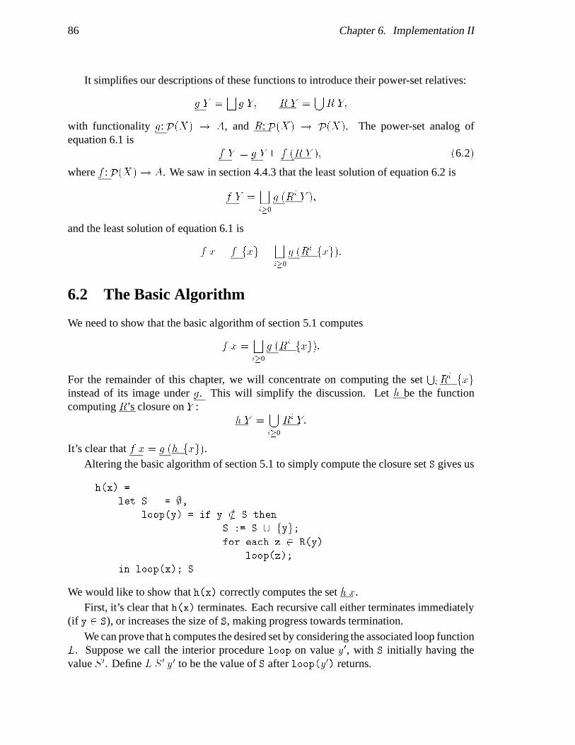
86 Chapter 6. Implementation II
It simplifies our descriptions of these functions to introduce their power-set relatives:
g Y =Gg Y; R Y =
[R Y;
with functionality g:P(X) ! A, and R:P(X) ! P(X). The power-set analog ofequation 6.1 is
f Y = g Y t f (R Y ); (6:2)
where f :P(X)! A. We saw in section 4.4.3 that the least solution of equation 6.2 is
f Y =Gi�0
g (Ri Y );
and the least solution of equation 6.1 is
f x = f fxg =Gi�0
g (Ri fxg):
6.2 The Basic Algorithm
We need to show that the basic algorithm of section 5.1 computes
f x =Gi�0
g (Ri fxg):
For the remainder of this chapter, we will concentrate on computing the setS
iRi fxg
instead of its image under g. This will simplify the discussion. Let h be the functioncomputing R’s closure on Y :
h Y =[i�0
Ri Y:
It’s clear that f x = g (h fxg).Altering the basic algorithm of section 5.1 to simply compute the closure set S gives us
h(x) =
let S = ;,loop(y) = if y =2 S then
S := S [ fyg;
for each z 2 R(y)
loop(z);
in loop(x); S
We would like to show that h(x) correctly computes the set h x.First, it’s clear that h(x) terminates. Each recursive call either terminates immediately
(if y 2 S), or increases the size of S, making progress towards termination.We can prove that h computes the desired set by considering the associated loop function
L. Suppose we call the interior procedure loop on value y0, with S initially having thevalue S 0. Define L S 0 y0 to be the value of S after loop(y0) returns.

6.3. The Aggressive-Cutoff Algorithm 87
The procedure loop(y) recursively explores the subtree rooted at y in a depth-firstorder, where R can be viewed as the “sons-of” function. However, loop cuts off the searchwhen it arrives at a node in the set S. So, we can intuitively see that L S y returns thetree explored from y, stopping at elements in S. The h function, on the other hand, can beviewed as a complete breadth-first search from its argument. This leads us to the followingtheorem:
Theorem 13 L S y [ h S = h fyg [ h S:
Proof:
1. L S y [ hS � h fyg [ hS:During the execution of loop(y), all elements added to S are produced by chainsof R applications, starting with y, hence each such element must be in y’s closure,h fyg. So,
L S y � h fyg [ S � h fyg [ h S:
The inclusion follows.
2. h fyg [ hS � L S y [ hS:Proof by negation. Suppose z 2 h fyg � (L S y [ h S). Now z 2 h fyg meansthere is a sequence s0; . . . ; sn such that s0 = y, sn = z, and si+1 2 Rsi (that is, thereis a sequence of R applications leading from y to z). Since z =2 h S, we know thatnone of the si are in S — if one was, then its descendant z would have to be in theclosure. Since z =2 LS y, we know sn�1 =2 LS y. However, sn�1 isn’t in the initial Sset, so if it were ever added to S, loop would recurse over its children R sn�1, whichincludes z, and so z would have been added to S. In a similar fashion, we can derive
z =2 L S y ) sn�1 =2 L S y ) � � � ) s1 =2 L S y ) y =2 L S y:
But, clearly y 2 L S y. Contradiction.
Q.E.D.
We can finish off h with the following corollary:
Corollary 14 h(x) = h fxg
Proof: This follows from the previous theorem, h(x) = L ; x, and h ; = ;.
6.3 The Aggressive-Cutoff Algorithm
If we similarly abstract the basic structure of the aggressive-cutoff algorithm of section 5.2,we get the procedure:
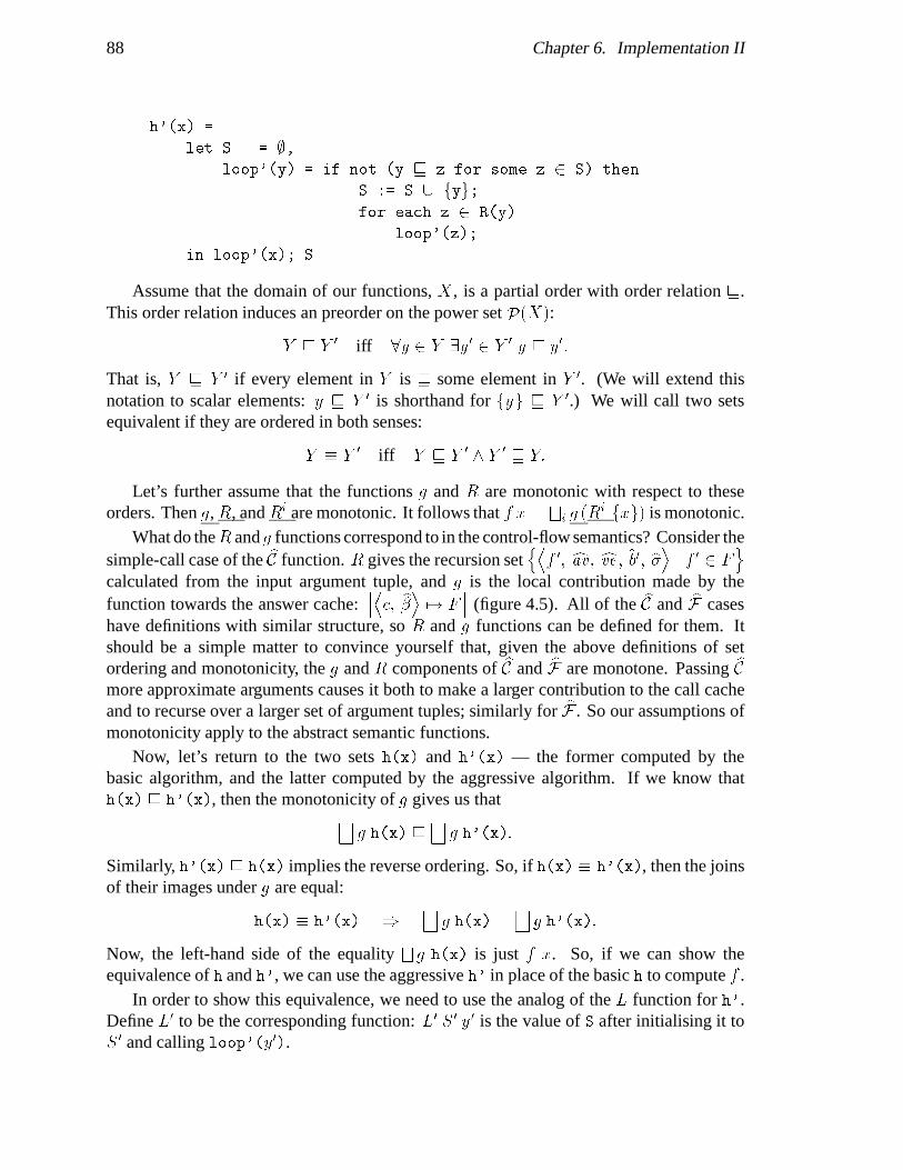
88 Chapter 6. Implementation II
h'(x) =
let S = ;,
loop'(y) = if not (y v z for some z 2 S) then
S := S [ fyg;
for each z 2 R(y)
loop'(z);
in loop'(x); S
Assume that the domain of our functions, X , is a partial order with order relation v.This order relation induces an preorder on the power set P(X):
Y v Y 0 iff 8y 2 Y 9y0 2 Y 0 y v y0:
That is, Y v Y 0 if every element in Y is v some element in Y 0. (We will extend thisnotation to scalar elements: y v Y 0 is shorthand for fyg v Y 0.) We will call two setsequivalent if they are ordered in both senses:
Y � Y 0 iff Y v Y 0 ^ Y 0 v Y:
Let’s further assume that the functions g and R are monotonic with respect to theseorders. Then g, R, and Ri are monotonic. It follows that f x =
Fi g (R
i fxg) is monotonic.What do theR and g functions correspond to in the control-flow semantics? Consider the
simple-call case of the bC function. R gives the recursion setnDf 0; cav ; cve ; b0; b�E j f 0 2 F
ocalculated from the input argument tuple, and g is the local contribution made by thefunction towards the answer cache:
hDc; b�E 7! F
i(figure 4.5). All of the bC and bF cases
have definitions with similar structure, so R and g functions can be defined for them. Itshould be a simple matter to convince yourself that, given the above definitions of setordering and monotonicity, the g and R components of bC and bF are monotone. Passing bCmore approximate arguments causes it both to make a larger contribution to the call cacheand to recurse over a larger set of argument tuples; similarly for bF . So our assumptions ofmonotonicity apply to the abstract semantic functions.
Now, let’s return to the two sets h(x) and h'(x) — the former computed by thebasic algorithm, and the latter computed by the aggressive algorithm. If we know thath(x) v h'(x), then the monotonicity of g gives us that
Gg h(x) v
Gg h'(x):
Similarly, h'(x) v h(x) implies the reverse ordering. So, if h(x) � h'(x), then the joinsof their images under g are equal:
h(x) � h'(x) )Gg h(x) =
Gg h'(x):
Now, the left-hand side of the equalityFg h(x) is just f x. So, if we can show the
equivalence of h and h', we can use the aggressive h' in place of the basic h to compute f .In order to show this equivalence, we need to use the analog of the L function for h'.
Define L0 to be the corresponding function: L0 S0 y0 is the value of S after initialising it toS0 and calling loop'(y0).
6.3. The Aggressive-Cutoff Algorithm 89
Theorem 15 L0 S y [ h S � h fyg [ h S:
Proof:The proof is similar to the previous proof for the basic algorithm, using v in place of 2.
1. L0 S y [ h S v h fyg [ h S:During the execution of loop'(y), all elements added to S are of produced by chainsof R applications, starting with y, hence each such element must be in y’s closure,h fyg. So,
L0 S y � h fyg [ S � h fyg [ h S:
Clearly, h S � h fyg [ h S as well, so
L0 S y [ h S � h fyg [ h S;
which in turn impliesL0 S y [ h S v h fyg [ h S:
2. h fyg [ h S v L0 S y [ h S:Proof by negation. Suppose 9z 2 h fyg � h S such that z 6v L0 S y [ h S. Sincez 2 h fyg, there is a sequence s0; . . . ; sn such that s0 = y, sn = z, and si+1 2 R si(that is, there is a sequence of R applications leading from y to z). Now, sincez 6v h S, we know that 8i si 6v S — if some si were v S, then by the monotonicityof R, its descendant z would have to be v the closure h S.
Since z 6v L0Sy, we know sn�1 6v L0Sy. To see this, suppose that sn�1 v x 2 L0Sy,for some x. Since sn�1 6v S, we know that x =2 S, so xmust have been added toL0Syduring the execution of the algorithm. However, when loop' adds some elementx to S, it also recurses over x’s children R x. R is monotonic, so the recursion setR x includes some element w w z. Since loop' is called on w, the final value isguaranteed to be w w (either w is v some element already in S, or it is added toS itself; either way, the result set is w w), hence w z. So z v L0 S y, which is acontradiction. Hence sn�1 6v L0 S y.
We can apply this reasoning backwards along the si chain, giving us the series ofimplications:
z 6v L0Sy ) sn�1 6v L0Sy ) � � � ) s1 6v L0Sy ) y 6v L0Sy:
But, clearly y v L0 S y. Contradiction.
Q.E.D.
This theorem allows us to show that the aggressive-cutoff algorithm is equivalent to thebasic algorithm, with the following corollary:
Corollary 16 8y; h'(y) � h fyg.
90 Chapter 6. Implementation II
Proof: The previous theorem gives us
L0 ; y [ h ; � h fyg [ h ;:
h ; = ;, and h'(y) = L0 ; y, and the equivalence follows. Q.E.D.Now that we’ve established that the basic and aggressive-cutoff algorithms are equiva-
lent, we can implement the more efficient aggressive-cutoff algorithm and know that it willcompute the desired function.
6.4 The Time-Stamp Algorithm
It is fairly simple to show that the time-stamp algorithm is a conservative approximation tothe basic algorithm.
Suppose that the bC function is being applied to some simple-call tuple cs . Consider therecursion set R cs of FState tuples on which bC recursively applies bF . This is the set
n Dfi; cav ; cve ; cnb b c; b�E j 1 � i � n
o;
wherenf1; . . . ; fn
o= bA f b� cve . Changing to an algorithm that uses a single-threaded
implementation of the variable environment and store means that between the f1 call andthe f2 call, the store and variable environment could increase. So the actual values of theglobal variable environment and store present when the f2 call is made aren’t cve and b�, butsome values cve 2 w cve and b�2 w b�. This means we are actually calling F with the tupleDf2; cav ; cve 2;
cnb b c; b�2
EwDf2; cav ; cve ; cnb b c; b�E. Between the f2 call and the f3 call,
the globally modified cve and b� variables can again be increased. So the actual values of thevariable environment and store present when the f3 is made are some values cve 3 w cve2 andb�3 w b�2, and so forth for the successive calls to the rest of the fi. So the effective recursionset for the single-threaded implementation is
n Dfi; cav ; cve i;
cnb b c; b�i
Ej 1 � i � n
o:
Call this alternate recursion set R0cs . It’s clear that the cve i are all w cve and that the b�i are
all w b�, so each tuple in R0cs is w its counterpart in R cs . Thus we know R0 w R using
the ordering of the previous section.This is pervasively true throughout the bC and bF functions: the only change of making
the variable environment and store be global, single-threaded data structures is to shiftto recursion sets that are w their counterparts in the basic algorithm. So, returning toour simple f x = g x t
Ff (R x) model of the semantics functions, the single-threaded
algorithm computes the function defined by
f 0 x = g x tG
f 0 (R0 x);
which is justf 0 x =
Gi
g (R0i x):
6.4. The Time-Stamp Algorithm 91
Now, the basic recursion is computing the function
f x =Gi
g (Ri x):
As we discussed in the previous section, if R0 w R, then R0i w Ri. This plus themonotonicity of g gives us that
f 0 w f;
or that the single-threaded recursion safely approximates the basic recursion.

92 Chapter 6. Implementation II

Chapter 7
Applications I
The term “collection of hacks” is not meantto be pejorative. Some of my best friends arecollections of hacks.
— S. Fahlman
Once we’ve performed control-flow analysis on a program, we can use the informationgained to perform other data-flow analyses. Control-flow analysis by itself does not provideenough information to solve all the data-flow problems we might desire (we’ll discuss theselimitations in the following chapter), but we can still solve some useful problems.
In this chapter, we’ll consider three applications we can perform using control-flowinformation: induction-variable elimination, useless-variable elimination, and constantpropagation.
7.1 Induction-Variable Elimination
Induction-variable elimination is a technique used to transform array references withinloops into pointer incrementing operations. For example, suppose we have the followingC routine:
int a[50][30];
example() f
integer r, c;
for(r=0; r<50; r++)
for(c=0; c<30; c++)
a[r][c] = 4;
g
93

94 Chapter 7. Applications I
The example function assigns 4 to all the elements of array a. The array refer-ence a[r][c] on a byte addressed machine is equivalent to the address computationa+4*(c+30*r). This calculation requires two multiplications and two additions. How-ever, since the address value is linear in the c and r terms, we can cheaply compute theaddress computation incrementally.
example() f
integer *ptr;
for(ptr=a; ptr<a+1500; ptr++)
*ptr = 4;
g
The ptrvariable tracks the dependent valuea+4*(c+30*r). Induction-variableelimination(IVE) is a technique for automatically performing the above transformation. Classical IVEis treated in detail in the “Dragon” book [Aho+ 86].
Classical IVE for imperative languages such as C or Pascal begins by searching forbasic induction variables (BIVs). A BIV is a variable that is only altered in a loop byincrementing or decrementing it by constants. The r and c variables are BIVs in the aboveexample. In Scheme, the role of a single C BIV is played by a set of related Schemevariables, called a basic induction variable family. We use a set of Scheme variables in theplace of a single C variable because of the different ways that loop variables are updatedin the two languages. In C, a loop variable is updated multiple times within a loop byassigning to that single variable:
j=0;
while(test) f
j = j+1;
. . .j = j-4;
. . .j = j+2;
g
In Scheme or ML, an iteration variable is updated by rebinding it in a tail-recursive loop:
(letrec ((loop (� (j)
(if (not test)(let ((j' (+ j 1)))
. . .(let ((j% (- j' 4)))
. . .(loop (+ j% 2))))))))
(loop 0))

7.1. Induction-Variable Elimination 95
In the Scheme code, the variables fj; j'; j%g correspond to the C variable j.1 So, whereasIVE analysis in C searches for the basic induction variable j, the Scheme variant searchesfor the family fj; j'; j%g.
A basic induction variable (BIV) family is a set of variables B = fv1; . . . ; vng obeyingthe following constraints:
1. Every call site that calls one of the vi’s lambda expression may only call one lambdaexpression.
2. Each vi may only have definitions of the form b (constant b), and a + vj (vj 2 B,constant a). This corresponds to stating that vi’s lambda must be one of:
� Called from a call site that simply binds vi to a constant:((� (x vi z) . . . ) foo 3 bar).
� The continuation of a + call, with vj and a constant for addends:(+ vj a (� (vi) . . . )).
� The continuation of a - call, with vj and a constant for subtrahend and minuend:(- vj a (� (vi) . . . )).
� Called from a call site that simply binds vi to some vj , e.g.:((� (x vi z) . . . ) foo vj bar) (This is a special case of a = 0).
Given the control-flow information summarised by an abstract call cache function , it isfairly simple to compute sets of variables satisfying these constraints.
After finding BIVs, IVE analysis searches for dependent induction variables (DIVs) —variables whose values are affine functions of some other induction variable. The com-putations calculating these variables are then replaced with cheaper incremental updates.Again, the Scheme variant looks for families of variables dependent on BIV families, andthe emphasis is on binding updates instead of assignment updates.
A dependent induction variable (DIV) family is a set of variables D = fwig togetherwith a function f(n) = a+ b � n (a,b constant) and a BIV family B = fvig such that:
� For each wi, every definition of wi is wi = f (vj) for some vj 2 B.
We call the value f(vi) the dependent value.
We can introduce three sets of new variables, fzig, fxig, and fyig. The zi and xi
track the dependent value, and the yi are introduced as temporaries to help update the basicvariable. In the following description, we use for illustration the following piece of Schemecode:
1In fact, all three variables in the set would probably be named j by the programmer — there is no pointin distinguishing the names if they represent the same conceptual identifier at different points in the code. Sothe binding operations would look more like a real update: (let ((j (- j 4))) . . . ). However, by thetime the compiler begins to analyse the code, the compiler front-end has “alphatised” the three variables tohave distinct names.

96 Chapter 7. Applications I
(+ v1 4 (� (v2) . . . (* 3 v2 (� (w1) . . . ))))
BIVs v1 & v2
6 6
DIV w1 definedto be 3 � v2
6
with associated function f(n) = 3 � n.
We perform the following transformations on the code:
� Introduce zi into the vi lambda expression:Modify each lambda that binds one of the vi to simultaneously bind the correspondingvalue f (vi) to zi.Binding site (� (v2) . . . ) becomes:(� (v2 z2) . . . )
� Introduce code to compute zj = f(vj) from zi = f(vi)when vj is computed fromviAll call sites who have continuations binding one of the vi (i.e., call sites that step theBIV family) are modified to update the corresponding zi value. Temporary variablesxi and yi are used to serially compute the new values.Call site (+ v1 4 k) becomes:
(+ z1 12 (� (x2)
(+ v1 4 (� (y2)
(k y2 x2)))))
� Replace computation of DIV wi from vj with simple binding:Since zj = f (vj), we can remove the computation ofwj from vj , and simply bind wj
to zj . Dependent variable computation (* v2 3 (� (w1) . . . )) becomes:((� (w1) . . . ) z2) and z2 can be �-substituted for w1.
Notice that fwig [ fzig [ fxig now form a new BIV family, and may trigger off newapplications.
For example, consider the loop of figure 7.1(a). It is converted to the partial CPS of (b).Now, fng is a BIV family, and fmg is a DIV family dependent on fng, with f(n) = 3n. Awave of IVE transformation gives us the optimised result of (c). Analysis of (c) reveals thatf3n; 3n'; 3n%g is a BIV family, and fpg is a DIV family, with f (n) = 4+n. Another waveof IVE gives us (d). If we examine (d), we notice that 3n, 3n', and 3n% are never used,except to compute values for each other. Another analysis using control-flow information,useless-variable elimination, spots these useless variables; they can be removed, leavingthe optimised result of (e). (We’ll discuss useless-variable elimination in the next section.)
This example of figure 7.1 was produced by an IVE implementation that I wrote in Tusing the results produced by a 0CFA analysis.

7.1. Induction-Variable Elimination 97
(letrec ((f (� (n) (if (< n 50)
(if (= (aref a n) n) (f (+ n 1))
(block (print (+ 4 (* 3 n)))
(f (+ n 2))))))))
(f 0))(a) Before
(letrec ((f (� (n)
(if (< n 50)
(if (= (aref a n) n) (+ n 1 f)
(* 3 n (� (m) (+ 4 m (� (p) (print p)
(+ n 2 f))))))))))
(f 0))(b) Partial CPS conversion
(letrec ((f (� (n 3n)
(if (< n 50)
(if (= (aref a n) n)
(+ 3n 3 (� (3n')
(+ n 1 (� (n') (f n' 3n')))))
(+ 4 3n (� (p) (print p)
(+ 3n 6 (� (3n%)
(+ n 2 (� (n%)
(f n% 3n%))))))))))))
(f 0 0))(c) IVE wave 1
(letrec ((f (� (n 3n 3n+4)
(if (< n 50)
(if (= (aref a n) n)
(+ 3n+4 3 (� (3n+4')
(+ 3n 3 (� (3n') (+ n 1 (� (n')
(f n' 3n' 3n+4')))))))
(block (print 3n+4)
(+ 3n+4 6 (� (3n+4%)
(+ 3n 6 (� (3n%)
(+ n 2 (� (n%)
(f n% 3n% 3n+4%)))))))))))))
(f 0 0 4))(d) IVE wave 2
(letrec ((f (� (n 3n+4)
(if (< n 50)
(if (= (aref a n) n)
(+ 3n+4 3 (� (3n+4') (+ n 1 (� (n') (f n' 3n+4')))))
(block (print 3n+4)
(+ 3n+4 6 (� (3n+4%)
(+ n 2 (� (n%)
(f n% 3n+4%)))))))))))
(f 0 4))(e) After
Figure 7.1: Example IVE application
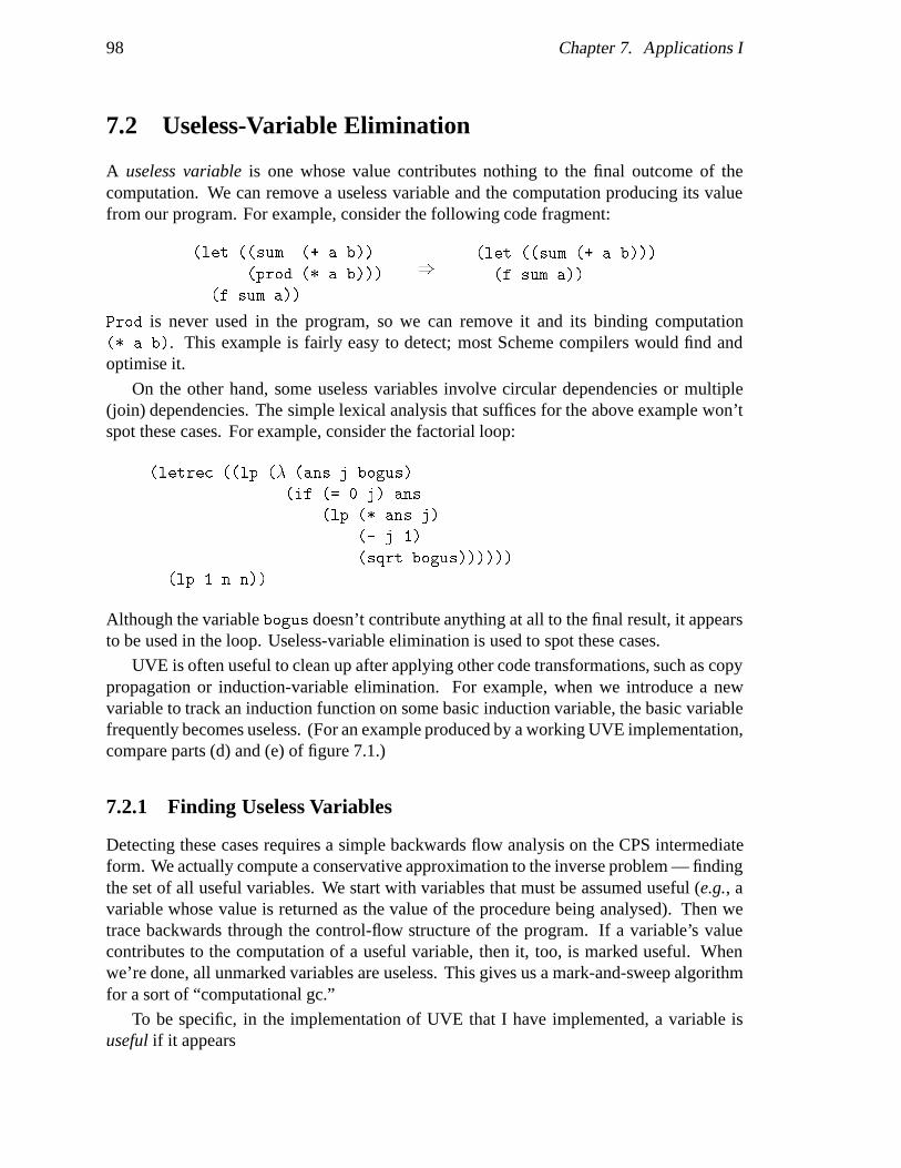
98 Chapter 7. Applications I
7.2 Useless-Variable Elimination
A useless variable is one whose value contributes nothing to the final outcome of thecomputation. We can remove a useless variable and the computation producing its valuefrom our program. For example, consider the following code fragment:
(let ((sum (+ a b))
(prod (* a b)))
(f sum a))
)(let ((sum (+ a b)))
(f sum a))
Prod is never used in the program, so we can remove it and its binding computation(* a b). This example is fairly easy to detect; most Scheme compilers would find andoptimise it.
On the other hand, some useless variables involve circular dependencies or multiple(join) dependencies. The simple lexical analysis that suffices for the above example won’tspot these cases. For example, consider the factorial loop:
(letrec ((lp (� (ans j bogus)
(if (= 0 j) ans
(lp (* ans j)
(- j 1)
(sqrt bogus))))))
(lp 1 n n))
Although the variable bogus doesn’t contribute anything at all to the final result, it appearsto be used in the loop. Useless-variable elimination is used to spot these cases.
UVE is often useful to clean up after applying other code transformations, such as copypropagation or induction-variable elimination. For example, when we introduce a newvariable to track an induction function on some basic induction variable, the basic variablefrequently becomes useless. (For an example produced by a working UVE implementation,compare parts (d) and (e) of figure 7.1.)
7.2.1 Finding Useless Variables
Detecting these cases requires a simple backwards flow analysis on the CPS intermediateform. We actually compute a conservative approximation to the inverse problem — findingthe set of all useful variables. We start with variables that must be assumed useful (e.g., avariable whose value is returned as the value of the procedure being analysed). Then wetrace backwards through the control-flow structure of the program. If a variable’s valuecontributes to the computation of a useful variable, then it, too, is marked useful. Whenwe’re done, all unmarked variables are useless. This gives us a mark-and-sweep algorithmfor a sort of “computational gc.”
To be specific, in the implementation of UVE that I have implemented, a variable isuseful if it appears

7.2. Useless-Variable Elimination 99
� in the function position of a call:(f 5 0)
� as the predicate in a conditional primop:(if p (� () . . . ) (� () . . . ))
� as the continuation of a primop:(+ 3 5 c)
� as an argument in a call to
– a side-effecting operation (output or store):(print a), (set-car! x y)
– an external procedure, or a primop whose continuationis an external procedure.
– a primop whose continuation binds a useful variable:(+ metoo 3 (� (used) . . . ))
– a lambda whose corresponding parameter is useful:((� (x used y) . . . ) 3 metoo 7)
The first three conditions spot variables used for control flow. The next two mark variableswhose value escapes, and must therefore be assumed useful. The final two recursiveconditions are the ones that cause the analysis to chain backwards through the control-flowgraph: if a variable is useful, then all the variables used to compute its value are useful.
7.2.2 Optimising Useless Variables
Once we have found the useless variables in a program, we can optimise the program intwo steps. In the first step, we remove all references to useless variables and eliminate alluseless computations (primop calls). In the second step, we remove useless variables fromtheir lambda lists where possible.
Removing useless variables from calls
In this phase, we globally remove all references to useless variables in our program. Ifa useless variable appears as an argument to a primop call, we remove the entire primopcomputation. For instance, suppose the useless variable x appears as an argument inthe primop call (+ x y k). By the definition of a useless variable, we know that thecontinuation k must bind the result of the addition to a useless variable, as well (if it didn’t,we’d have marked x as useful). This renders the addition operation useless, so we canremove it, replacing (+ x y k) with (k #f). The actual value passed to the continuation(we used #f here) is not important — remember that we are globally deleting all referencesto useless variables. Since the continuation k must bind the value #f to a useless variable,the value is guaranteed never to be referenced.
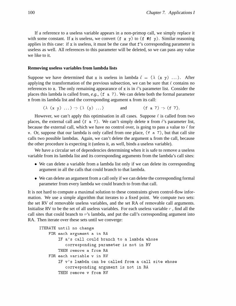
100 Chapter 7. Applications I
If a reference to a useless variable appears in a non-primop call, we simply replace itwith some constant. If x is useless, we convert (f x y) to (f #f y). Similar reasoningapplies in this case: if x is useless, it must be the case that f’s corresponding parameter isuseless as well. All references to this parameter will be deleted, so we can pass any valuewe like to it.
Removing useless variables from lambda lists
Suppose we have determined that x is useless in lambda ` = (� (x y) . . . ). Afterapplying the transformation of the previous subsection, we can be sure that ` contains noreferences to x. The only remaining appearance of x is in `’s parameter list. Consider theplaces this lambda is called from, e.g., (f a 7). We can delete both the formal parameterx from its lambda list and the corresponding argument a from its call:
(� (x y) . . . )) (� (y) . . .) and (f a 7)) (f 7).
However, we can’t apply this optimisation in all cases. Suppose ` is called from twoplaces, the external call and (f a 7). We can’t simply delete x from `’s parameter list,because the external call, which we have no control over, is going to pass a value to ` forx. Or, suppose that our lambda is only called from one place, (f a 7), but that call sitecalls two possible lambdas. Again, we can’t delete the argument a from the call, becausethe other procedure is expecting it (unless it, as well, binds a useless variable).
We have a circular set of dependencies determining when it is safe to remove a uselessvariable from its lambda list and its corresponding arguments from the lambda’s call sites:
� We can delete a variable from a lambda list only if we can delete its correspondingargument in all the calls that could branch to that lambda.
� We can delete an argument from a call only if we can delete the corresponding formalparameter from every lambda we could branch to from that call.
It is not hard to compute a maximal solution to these constraints given control-flow infor-mation. We use a simple algorithm that iterates to a fixed point. We compute two sets:the set RV of removable useless variables, and the set RA of removable call arguments.Initialise RV to be the set of all useless variables. For each useless variable v , find all thecall sites that could branch to v’s lambda, and put the call’s corresponding argument intoRA. Then iterate over these sets until we converge:
ITERATE until no change
FOR each argument a in RA
IF a's call could branch to a lambda whose
corresponding parameter is not in RV
THEN remove a from RA
FOR each variable v in RV
IF v's lambda can be called from a call site whose
corresponding argument is not in RA
THEN remove v from RV
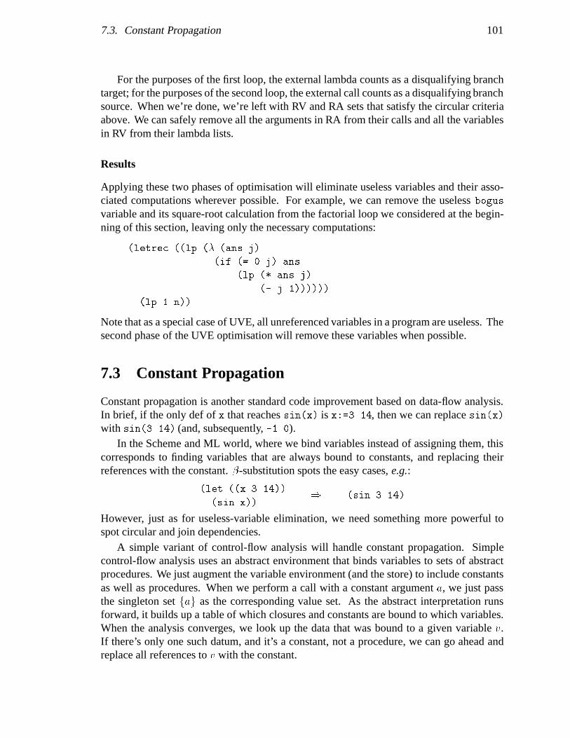
7.3. Constant Propagation 101
For the purposes of the first loop, the external lambda counts as a disqualifying branchtarget; for the purposes of the second loop, the external call counts as a disqualifying branchsource. When we’re done, we’re left with RV and RA sets that satisfy the circular criteriaabove. We can safely remove all the arguments in RA from their calls and all the variablesin RV from their lambda lists.
Results
Applying these two phases of optimisation will eliminate useless variables and their asso-ciated computations wherever possible. For example, we can remove the useless bogus
variable and its square-root calculation from the factorial loop we considered at the begin-ning of this section, leaving only the necessary computations:
(letrec ((lp (� (ans j)
(if (= 0 j) ans
(lp (* ans j)
(- j 1))))))
(lp 1 n))
Note that as a special case of UVE, all unreferenced variables in a program are useless. Thesecond phase of the UVE optimisation will remove these variables when possible.
7.3 Constant Propagation
Constant propagation is another standard code improvement based on data-flow analysis.In brief, if the only def of x that reaches sin(x) is x:=3.14, then we can replace sin(x)with sin(3.14) (and, subsequently, -1.0).
In the Scheme and ML world, where we bind variables instead of assigning them, thiscorresponds to finding variables that are always bound to constants, and replacing theirreferences with the constant. �-substitution spots the easy cases, e.g.:
(let ((x 3.14))
(sin x))) (sin 3.14)
However, just as for useless-variable elimination, we need something more powerful tospot circular and join dependencies.
A simple variant of control-flow analysis will handle constant propagation. Simplecontrol-flow analysis uses an abstract environment that binds variables to sets of abstractprocedures. We just augment the variable environment (and the store) to include constantsas well as procedures. When we perform a call with a constant argument a, we just passthe singleton set fag as the corresponding value set. As the abstract interpretation runsforward, it builds up a table of which closures and constants are bound to which variables.When the analysis converges, we look up the data that was bound to a given variable v.If there’s only one such datum, and it’s a constant, not a procedure, we can go ahead andreplace all references to v with the constant.

102 Chapter 7. Applications I
Chapter 8
The Environment Problem and ReflowAnalysis
In this chapter, we’ll examine the limits of simple control-flow analysis. Then we’ll developan extension, called reflow analysis, to move beyond these limits. In the following twochapters, we’ll look at some optimisations that can be performed with reflow analysis.
The work discussed in these next three chapters is not supported by the kind of carefulformal development and proofs of correctness that I’ve shown for the simple control-flowanalysis in the previous chapters. This work must be taken simply as interesting ideasthat have not yet been backed up with rigorous mathematics. With reflow analysis, we’vearrived at my research frontier as of the writing of this dissertation.
Future work could include a better theoretical characterisation of reflow analysis, andproofs of conservative abstraction and computability for reflow-based optimisations. Isuspect that this sort of work would be carried out in basically the same fashion as the workon simple control-flow analysis in chapter 4.
8.1 Limits of Simple Control-Flow Analysis
At the start of this dissertation, I told the following story: Data-flow analyses require acontrol-flow graph. Scheme programs don’t have static control-flow graphs. But, if wecould somehow recover a good approximation of the control-flow graph, we could use it toperform all the classical data-flow analyses.
It turns out that this is somewhat optimistic. While control-flow analysis does enablesome classical data-flow analyses — such as the ones we just developed in the last chapter— another class of applications cannot be handled this way.
This is the class of analyses that require detailed environment information. Classicaldata-flow analyses assume a single, flat environment over the program text. Assignmentsand references to global variables are the conduits through which computed values flowthrough the program. Thus any two references to the same variable refer to the same bindingof that variable. This is the model provided by assembly code.
103
104 Chapter 8. The Environment Problem and Reflow Analysis
The intermediate representation we are using, CPS applicative-order �-calculus, isdifferent. Here, we can have simultaneous multiple bindings of a single variable. Forinstance, consider the following puzzle:
(let ((f (� (x h) (if (zero? x) (h) (� () x)))))
(f 0 (f 3 '#f)))
The first call to f, (f 3 '#f), returns a closure over (� () x) in environment�[[x]] 7! 3
�.
This closure is then used as an argument in the second, outer call to f, where it is boundto h. Suppose we naively picked up information from the conditional (zero? x) test, andflowed the information x = 0 and x 6= 0 down the two arms of the if to be picked up byreferences to x. This would work in the single flat environment model of assembler. Inthis Scheme puzzle, however, we are undone by the power of lambda. Suppose that ourcontour abstraction maps the contours allocated by the two calls to f to the same abstractcontour. After ensuring that x = 0 in the then arm of the if, we jump off to h = (� () x),and evaluate a reference to x, which inconveniently persists in evaluating to 3, not 0. Theone variable has two simultaneous bindings. We tested one binding and then referencedthe other. Confusing the two bindings of the same variable can lead us to draw incorrectconclusions.
This problem prevents us from using plain control-flow analysis to perform importantflow analysis optimisations for Scheme, such as type recovery. In type recovery, we wouldlike to perform deduction of the form:
;;; references to x in f are int refs
(if (integer? x) (f) (g))
Unfortunately, as demonstrated above, we can’t make such inferences.The problem arises because of lambda’s ability to create multiple environments over a
given context. Analyses such as type recovery depend upon keeping these environmentsdistinct; computable procedural approximations depend upon folding these environmentstogether. This basic conundrum is what I call the “environment problem.”
Only certain data-flow analyses are affected by the environment problem. The keyproperty determining this is the direction in which the iterative analysis moves through theapproximation lattice. In control-flow analysis or useless-variable elimination the analysisstarts with an overly precise value and incrementally weakens it until it converges; allmotion in the approximate lattice is in the direction of more approximate values. So,identifying two contours together simply causes further approximation, which is safe.
With an analysis like type recovery, however, our analysis moves in both directionsalong the type lattice as the analysis proceeds, and this is the source of the environmentproblem. In type recovery, we are passing around statements about the types of the valuesbound to specific variables. When two different calls to a procedure, each passing argumentsof different types, bind a variable in the same abstract contour, the types are joined together— moving through the type lattice in the direction of increasing approximation. However,passing through a conditional test causes type information to be narrowed down — moving

8.2. Reflow Analysis and Temporal Distinctions 105
in the direction of increasing precision. Unfortunately, while it is legitimate to narrow downa variable’s type in a single exact contour, it is not legitimate to narrow down its type in thecorresponding abstract contour — other bindings that are identified together in the sameabstract contour are not constrained by the type test. This is the heart of the problem withthe above puzzle.
In general, then, the simple abstraction techniques of chapters 3–7 yield correct, con-servative, safe analyses only when the analysis moves through its answer lattice solely inthe direction of increasing approximation. Moving beyond this requires something new.
8.2 Reflow Analysis and Temporal Distinctions
Our central problem is that we are identifying together different contours over the samevariable. We are forced to this measure by our desire to reduce an infinite number ofcontours down to a finite set.
For example, suppose we know that abstract procedure f =D[[`:(� (x) . . . )]]; b�E is
called from 3 different call sites, c1, c2 and c3. In 1CFA, all the contours allocated whenentering ` will be folded down to 3 abstract contours, one of fc1; c2; c3g. Now, suppose weare in the middle of an abstract interpretation, and we have a call to f from c2:(g z). Wedesire to track information associated with this binding of x. First, notice that the contourabstraction already distinguishes this binding of x from all the bindings that abstract tocontour c1 or c3. We get into trouble from two sources: (1) previous bindings of x in thesame abstract contour c2, and (2) future bindings of x in the same abstract contour c2. Inother words, we won’t confuse this binding with any bindings made in abstract contours c1
or c3, but we could confuse it with any made by other calls from c2 — either calls previouslymade during program execution, or calls to be made in the future.
So, if we want to track the information associated with a general abstract binding ofa variable, we need a way to distinguish it from past and future bindings made under thesame abstract contour. This is the key to an iterative technique called reflow analysis.
We will start the program up in the middle of its execution, running it forward fromthe c2 call to `. We’ll call this re-interpretation of the program from some mid-point asingle “reflow.” On this particular entry to `, we’ll allocate a special contour, c02, that willdistinguish the c2 contour being tracked from the other c2 calls, past or future, that wouldallocate the same abstract contour. It’s the c02 binding of x that we will track.
Now, it is quite likely that there is already a h[[x]]; c2i binding in cve when we start theprogram up in mid-stride, but this abstract binding is distinct from the special c02 bindingwe are uniquely allocating at the beginning of this reflow. Further, any future entries to `
from c2 during this reflow will allocate the ordinary c2 contour, merging them in with thepreviously-recorded c2 binding, but remaining distinct from the special c02 binding we aretracking during this reflow. In this manner, we are distinguishing the reflow’s initial bindingfrom other bindings, past and future, that would otherwise abstract to the same binding.
This allows us to track the special c02 contour’s variable bindings during the programreflow. Suppose we are running the program forward, and we come to a reference to x,
106 Chapter 8. The Environment Problem and Reflow Analysis
bound in contour c02. We know this isn’t a binding of x established by any call to ` fromeither c1 or c3, else the contour would be c1 or c3. We also know that this isn’t a binding ofx caused by a call to ` from c2 that occurred either before or after the call we’re tracking,because those calls get allocated contour c2 — the special contour c02 is allocated only once.So we’ve managed to keep this binding of x distinct from its other bindings.
This means that as we run the program forward, whenever we test x, if the test occursin contour c02, we can track the information produced by the test. If the test is to some otherbinding of x, we ignore it. Whenever we arrive at a reference to x, if the reference occursin contour c02, we can record the information. If the reference is to some other binding of x,we ignore it. Tracking the c02 binding of x is safe, because we’ve isolated it from any of itsother possible bindings.
Since we’ve only tracked one of `’s possible contours, we must repeat the analysis forthe two other abstract contours allocated to `. So we restart the program from the call c1,allocating special contour c01, and track the binding of x in that special contour. Finally, werestart the analysis from the c3 call.
One detail we must handle is how to restart the analysis in mid-stream. What valuesdo we use for cve and b�, for example? A simple solution is to take values for cve and b� thatsafely approximate any value they could have had at that point of the interpretation. Wecould, for example, use the final values of cve and b� after performing a control-flow analysisof our program using the time-stamp approximate algorithm discussed in section 5.3. Thesevalues are guaranteed to approximate any cve or b� that could arise during interpretation ofthe program. So, we can safely use them to restart the program from any call context
Dc; b�E
that appears in the domain of the call cache produced by the analysis.

Chapter 9
Applications II: Type Recovery
Strong types are for weak minds.— anon.
In this chapter we’ll examine in detail an optimisation that requires reflow analysis:type recovery. The full-blown semantics machinery for type recovery is fairly complex,and I recommend browsing or skipping these sections on a first reading.
9.1 Type Recovery
Scheme is a latently typed language [Rees+ 86]. This means that unlike statically typedlanguages such as ML or Pascal, types are associated only with run-time values, not withvariables. A variable can potentially be bound to values of any type, and type tests canbe performed at run time to determine the execution path through a program. This givesthe programmer an extremely powerful form of polymorphism without requiring a verbosesystem of type declarations.
This power and convenience is not without substantial cost, however. Since run-timebehavior can determine which values are bound to a given variable, precisely determiningthe type of a given reference to a variable is undecidable at compile time. For example,consider the following fragment of Scheme code:
(let ((x (if (oracle) 3 'three)))
(f x))
The reference to x in the subexpression (f x) could have any one of the types integer,symbol, integer+symbol, or bottom, depending on whether the oracle always returns true,always returns false, sometimes returns both, or never returns at all, respectively. Of course,determining the oracle’s behavior at compile time is, in general, undecidable.
We can use data-flow analysis to recover a conservative approximation of the typeinformation implicit in a program’s structure. This analysis performs a kind of type
107

108 Chapter 9. Applications II: Type Recovery
inference. Since the term “type inference” is commonly used to refer to the generationof static type assignments for variables, I will instead refer to the type analysis performedby this technique as type recovery: the recovery of type information from the control andenvironment structure of a program.
9.1.1 Sources of Type Information
Type information in Scheme programs can be statically recovered from three sources:conditional branches, applications of primitive operations, and user declarations.
Conditional Branches
Consider a simple version of the Scheme equal? predicate:
(define (equal? a b)
(cond ((number? a)
(and (number? b) (= a b)))
((pair? a)
(and (pair? b)
(equal? (car a) (car b))
(equal? (cdr a) (cdr b))))
(else (eq? a b))))
There are three arms in the cond form. References to a down the first arm are guaranteed tohave type number. Furthermore, in the numeric comparison form, (= a b), an assumptioncan be made that b is also a number, since the and guarantees that control reaches thecomparison only if (number? b) is true. Similarly, we can infer that references to a inthe second arm of the cond have the pair type and, less usefully, that references to a inthe third arm of the cond do not have either type pair or number. It is important to realisefrom this example that Scheme type recovery assigns types not to variables, but to variablereferences. The references to a in the different arms of the cond all have different types.
Type recovery of this sort can be helpful to a Scheme compiler. If the compiler candetermine that the (= a b) form is guaranteed to compare only numbers, it can compilethe comparison without a run-time type check, gaining speed without sacrificing safety.Similarly, determining that the (car a), (car b), (cdr a), and (cdr b) forms are allguaranteed to operate on pairs allows the compiler to safely compile the car and cdr
applications without run-time type checks.
Primop Application
An obvious source of type information is the application of primops such as + and cons.Clearly the result of (cons a b) is a pair. In addition, we can recover information aboutthe type of subsequent references to primop arguments. For example, after the primop
9.1. Type Recovery 109
application (cdr p), references to p along the same control path can be assumed to havethe pair type.
As a simple example, consider the following Scheme expression:
(let* ((a (cdr b))
(q (char->integer (vector-ref a i))))
. . . (car b) . . . (+ q 2))
References to b occurring after the (cdr b) form are guaranteed to have the pair type —otherwise, the cdr application would have rendered the effect of the computation to beundefined. Hence, the subsequent (car b) application does not need to do a type check.Similarly, after evaluating the second clause of the let*, references to a have type vectorand references to i and q are small integers, because vector-ref requires an integerindex, and char->integer generates an integer result. Hence the compiler can omit alltype checks in the object code for (+ q 2), and simply open-code the addition.
In recovering information about the arguments to primops, we are essentially usinginformation from “hidden conditional tests” inside the primop. The semantics of a (dan-gerous) CPS car primop is:
(define (car p cont)
(if (pair? p) (cont (%car p))
($)))
where the subprimitive operation %car is only defined over cons cells, and ($) is a specialprimop denoting a computation with undefined effect. Computation proceeds through thecontinuation cont only in the then arm of the type test, so we may assume that p’s value isa cons cell while executing the continuation. Recovering the type information implied bycar reduces to recovering type information from conditional branches.
Of course, the compiler does not need to emit code for a conditional test if one armis ($). It can simply take the undefined effect to be whatever happens when the codecompiled for the other arm is executed. This reduces the entire car application to themachine operation %car.
A safe implementation of Scheme is one that guarantees to halt the computation as soonas a type constraint is violated. This can be modeled by replacing the ($) form in the elsearm of the car definition with a call to the run-time error handler:
(define (car p cont)
(if (pair? p) (cont (%car p))
(error)))
Of course, type information recovered about the arguments to a particular application ofcar may allow the conditional test to be determined at compile time, again allowing thecompiler to fold out the conditional test and error call, still preserving type-safety withoutthe run-time overhead of the type check.
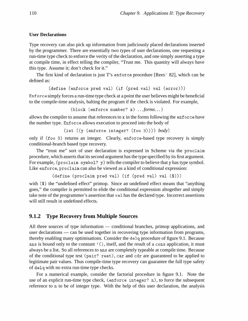
110 Chapter 9. Applications II: Type Recovery
User Declarations
Type recovery can also pick up information from judiciously placed declarations insertedby the programmer. There are essentially two types of user declarations, one requesting arun-time type check to enforce the verity of the declaration, and one simply asserting a typeat compile time, in effect telling the compiler, “Trust me. This quantity will always havethis type. Assume it; don’t check for it.”
The first kind of declaration is just T’s enforce procedure [Rees+ 82], which can bedefined as:
(define (enforce pred val) (if (pred val) val (error)))
Enforce simply forces a run-time type check at a point the user believes might be beneficialto the compile-time analysis, halting the program if the check is violated. For example,
(block (enforce number? x) . . . forms. . . )
allows the compiler to assume that references to x in the forms following the enforce havethe number type. Enforce allows execution to proceed into the body of
(let ((y (enforce integer? (foo 3)))) body)
only if (foo 3) returns an integer. Clearly, enforce-based type recovery is simplyconditional-branch based type recovery.
The “trust me” sort of user declaration is expressed in Scheme via the proclaim
procedure, which asserts that its second argument has the type specified by its first argument.For example, (proclaim symbol? y) tells the compiler to believe that y has type symbol.Like enforce, proclaim can also be viewed as a kind of conditional expression:
(define (proclaim pred val) (if (pred val) val ($)))
with ($) the “undefined effect” primop. Since an undefined effect means that “anythinggoes,” the compiler is permitted to elide the conditional expression altogether and simplytake note of the programmer’s assertion that val has the declared type. Incorrect assertionswill still result in undefined effects.
9.1.2 Type Recovery from Multiple Sources
All three sources of type information — conditional branches, primop applications, anduser declarations — can be used together in recovering type information from programs,thereby enabling many optimisations. Consider the delq procedure of figure 9.1. Becauseans is bound only to the constant '(), itself, and the result of a cons application, it mustalways be a list. So all references to ans are completely typeable at compile time. Becauseof the conditional type test (pair? rest), car and cdr are guaranteed to be applied tolegitimate pair values. Thus compile-time type recovery can guarantee the full type safetyof delq with no extra run-time type checks.
For a numerical example, consider the factorial procedure in figure 9.1. Note theuse of an explicit run-time type check, (enforce integer? n), to force the subsequentreference to n to be of integer type. With the help of this user declaration, the analysis
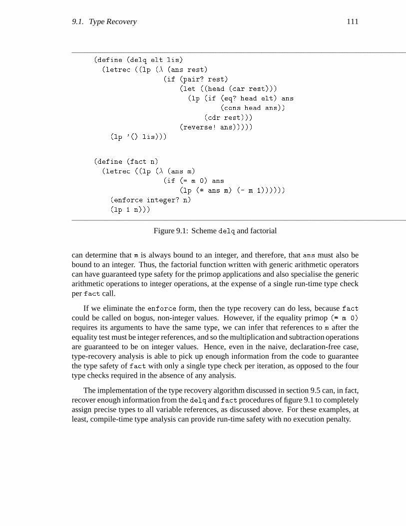
9.1. Type Recovery 111
(define (delq elt lis)
(letrec ((lp (� (ans rest)
(if (pair? rest)
(let ((head (car rest)))
(lp (if (eq? head elt) ans
(cons head ans))
(cdr rest)))
(reverse! ans)))))
(lp '() lis)))
(define (fact n)
(letrec ((lp (� (ans m)
(if (= m 0) ans
(lp (* ans m) (- m 1))))))
(enforce integer? n)
(lp 1 n)))
Figure 9.1: Scheme delq and factorial
can determine that m is always bound to an integer, and therefore, that ans must also bebound to an integer. Thus, the factorial function written with generic arithmetic operatorscan have guaranteed type safety for the primop applications and also specialise the genericarithmetic operations to integer operations, at the expense of a single run-time type checkper fact call.
If we eliminate the enforce form, then the type recovery can do less, because fact
could be called on bogus, non-integer values. However, if the equality primop (= m 0)
requires its arguments to have the same type, we can infer that references to m after theequality test must be integer references, and so the multiplication and subtraction operationsare guaranteed to be on integer values. Hence, even in the naive, declaration-free case,type-recovery analysis is able to pick up enough information from the code to guaranteethe type safety of fact with only a single type check per iteration, as opposed to the fourtype checks required in the absence of any analysis.
The implementation of the type recovery algorithm discussed in section 9.5 can, in fact,recover enough information from the delq and fact procedures of figure 9.1 to completelyassign precise types to all variable references, as discussed above. For these examples, atleast, compile-time type analysis can provide run-time safety with no execution penalty.

112 Chapter 9. Applications II: Type Recovery
9.2 Quantity-based Analysis
Type recovery is an example of what I call a quantity-based analysis. Consider the Schemeexpression
(if (< j 0) (- j) j)
Whatever number j names, we know that it is negative in the then-arm of the if expression,and non-negative in the else-arm. In short, we are associating an abstract property of j’svalue (its sign) with control points in the program. It is important to realize that we aretracking information about quantities (j’s value), not variables (j itself). For example,consider the following expression:
(let ((i j)) (if (< j 0) (foo i)))
Clearly, the test involving j determines information about the value of i since they bothname the same quantity. In a quantity-based analysis, information is tracked for quantities,and quantities can be named by multiple variables. This information can then be associatedwith the variable references appearing in the program. For the purposes of keeping track ofthis information, we need names for quantities; variables can then be bound to these quantitynames (which are called qnames), which in turn have associated abstract properties.
In principle, calls to primops such as + or cons create new qnames since these operationsinvolve the creation of new computational quantities. On the other hand, lambda bindingsimply involves the binding of a variable to an already existing qname. In practice, extraqnames often must be introduced since it can be difficult to determine at compile-timewhich qname a variable is bound to. Consider, for example, the following procedure:
(define (foo x y) (if (integer? x) y 3))
It might be the case that all calls to foo are of the form (foo a a), in which case x and y
can refer to the same qname. But if the analysis cannot determine this fact at compile time,x and y must be allocated two distinct qnames; hence determining information about x’svalue will not shed light on y’s value.
As another example, consider the vector reference in the expression:
(let ((y (vector-ref vec i))) . . .)
Now, y is certainly bound to an existing quantity, but it is unlikely that a compile-timeanalysis will be able to determine which one. So, a new qname must be assigned to y’sbinding.
In general, then, a conservative, computable, quantity-based analysis approximates thetracking of information on run-time values by introducing new qnames whenever it isunable to determine to which existing qname a variable is bound. These extra qnames limitthe precision of the analysis, but force the analysis to err conservatively.
9.3 Exact Type Recovery
Following the NSAS approach, the first step towards type recovery is to define an exactanalysis that will capture the notion of type recovery. Our exact semantics, which we will

9.3. Exact Type Recovery 113
call ETREC, does not have to be computable; we will concern ourselves with a computableapproximation in section 9.4.
For the purposes of this chapter, we’ll drop back to the simpler, less formal semantics ofchapter 3. So the semantics will have no store or side-effects, run-time error checks will beomitted, we’ll gloss over the details of the nb gensym function, and the semantic functionswill be curried over their multiple arguments instead of taking single tuples. These featurescan be restored as we did going from the informal control-flow semantics of chapter 3 tothe formal semantics of chapter 4.
Exact type recovery gives us a type cache:
A type cache for a CPS Scheme programP is a function � that, for each variablereference r and each binding contour b over r, returns �hr; bi, a type of thevalue to which r could evaluate in contour b.
Once we’ve computed a type cache, we can easily find the type for any variable referencer:v in our program:
RefType[[r:v]] =Gb
�hr; bi:
Here we are joining in the type lattice all the various types that a reference r had in all itsvarious binding contexts. The least-upper bound of these types is a legitimate static typefor r.
9.3.1 Basic Structure
The ETREC semantics maps a CPS Scheme program to its type cache. Its structure,however, is very similar to a standard semantics for CPS Scheme. Before proceeding to thedetails of the type-recovery machinery, I’ll briefly sketch out this basic structure.
The sets Bas, Proc, and D are just as in the standard semantics of chapter 3. The domainof type caches, TCache, is the cpo of partial functions from variable-reference/contour pairsto types.
Bas = Z + ffalseg
Proc = (LAM � BEnv) + PRIM + fstopg
D = Proc + Bas
TCache = (REF � CN)! Type
The basic environment and procedure structures are identical to the standard semanticscase. Note that we’ve named the VAR�CN set of variable bindings; this will be convenientlater on.
CN Contours
VB = VAR� CN
BEnv = LAB * CN
VEnv = VB * D

114 Chapter 9. Applications II: Type Recovery
In the ETREC semantics, the procedure and argument forms of a call expression areevaluated to values in D with the Av function, which is identical to the A function of thestandard semantics.
Av: ARG [ FUN ! BEnv ! VEnv * D
Av [[k]] � ve = K k
Av [[prim]] � ve = prim
Av [[`]] � ve = h`; �i
Av [[v]] � ve = ve hv; �(binder v)i
Procedure calls are handled by the C and F functions.
C: CALL ! BEnv ! VEnv ! QEnv ! TTab ! TCache
C [[(f a1 . . . an)]] � ve qe � =
� t F f 0 av qv ve qe � 0
where av#i = Av ai � ve
f 0 = Av f � ve
� 0 = f 2 REF �! � u >�Aq f � qe 7! type=proc
�otherwise �
� =�hri; � (binder vi)i 7! � (Aq vi � qe)
�8f; ai 2 REF
where ai = [[ri:vi]] and f = [[r0:v0]]
qv#i = ai 2 REF �! Aq ai � qe (quantity)otherwiseAt ai (type)
C takes five arguments: a call expression, the lexical contour environment �, the variableenvironment ve , and two others used for type recovery. C processes the first three argumentsjust as in the standard semantics case; we will return to the processing of the type informationin the next subsection.
The F function applies procedures to arguments.
F: Proc ! D� ! (Quant + Type)� ! VEnv ! QEnv ! TTab ! TCache
F h[[`:(� (v1 . . . vn) c)]]; �i av qv ve qe � =
C c �0 ve 0 qe 00 � 0
where b = nb
�0 = ��` 7! b
�ve 0 = ve
�hvi; bi 7! av#i
�qe 0 = qe
�hvi; bi 7! qv#i
�8i 3 qv#i 2 Quant (*)
qe 00 = qe 0�hvi; bi 7! hvi; bi
�� 0 = �
�hvi; bi 7! qv#i
�)8i 3 qv#i 2 Type (**)
Besides the extra arguments used for tracking type information, qv , qe , and � , and theirassociated processing, F is identical to the standard semantics case.
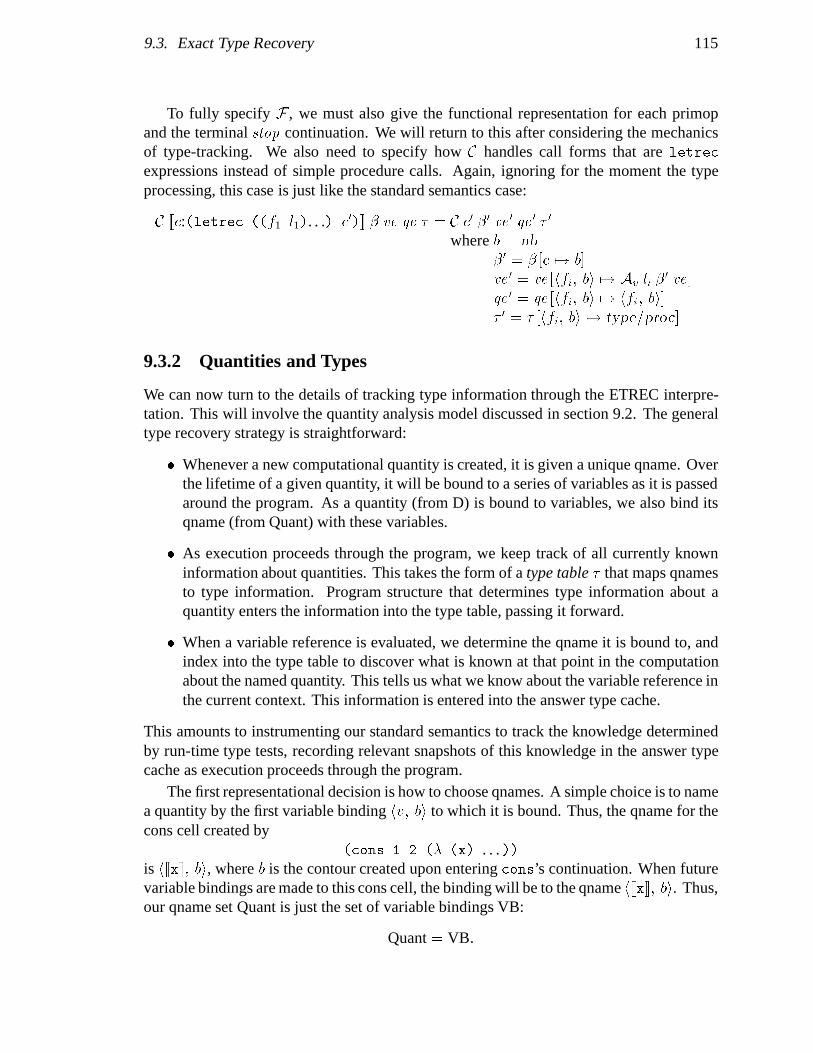
9.3. Exact Type Recovery 115
To fully specify F , we must also give the functional representation for each primopand the terminal stop continuation. We will return to this after considering the mechanicsof type-tracking. We also need to specify how C handles call forms that are letrec
expressions instead of simple procedure calls. Again, ignoring for the moment the typeprocessing, this case is just like the standard semantics case:
C [[c:(letrec ((f1 l1). . .) c0)]] � ve qe � = C c0 �0 ve 0 qe 0 � 0
where b = nb
�0 = ��c 7! b
�ve 0 = ve
�hfi; bi 7! Av li �
0 ve�
qe 0 = qe�hfi; bi 7! hfi; bi
�� 0 = �
�hfi; bi 7! type=proc
�
9.3.2 Quantities and Types
We can now turn to the details of tracking type information through the ETREC interpre-tation. This will involve the quantity analysis model discussed in section 9.2. The generaltype recovery strategy is straightforward:
� Whenever a new computational quantity is created, it is given a unique qname. Overthe lifetime of a given quantity, it will be bound to a series of variables as it is passedaround the program. As a quantity (from D) is bound to variables, we also bind itsqname (from Quant) with these variables.
� As execution proceeds through the program, we keep track of all currently knowninformation about quantities. This takes the form of a type table � that maps qnamesto type information. Program structure that determines type information about aquantity enters the information into the type table, passing it forward.
� When a variable reference is evaluated, we determine the qname it is bound to, andindex into the type table to discover what is known at that point in the computationabout the named quantity. This tells us what we know about the variable reference inthe current context. This information is entered into the answer type cache.
This amounts to instrumenting our standard semantics to track the knowledge determinedby run-time type tests, recording relevant snapshots of this knowledge in the answer typecache as execution proceeds through the program.
The first representational decision is how to choose qnames. A simple choice is to namea quantity by the first variable binding hv; bi to which it is bound. Thus, the qname for thecons cell created by
(cons 1 2 (� (x) . . .))is h[[x]]; bi, where b is the contour created upon entering cons’s continuation. When futurevariable bindings are made to this cons cell, the binding will be to the qname h[[x]]; bi. Thus,our qname set Quant is just the set of variable bindings VB:
Quant = VB:
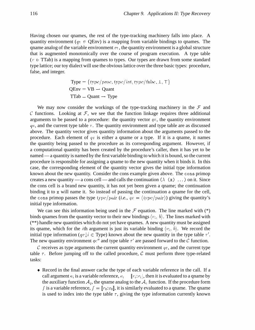
116 Chapter 9. Applications II: Type Recovery
Having chosen our qnames, the rest of the type-tracking machinery falls into place. Aquantity environment (qe 2 QEnv) is a mapping from variable bindings to qnames. Theqname analog of the variable environment ve , the quantity environment is a global structurethat is augmented monotonically over the course of program execution. A type table(� 2 TTab) is a mapping from qnames to types. Our types are drawn from some standardtype lattice; our toy dialect will use the obvious lattice over the three basic types: procedure,false, and integer.
Type = ftype=proc; type=int; type=false;?;>g
QEnv = VB * Quant
TTab = Quant ! Type
We may now consider the workings of the type-tracking machinery in the F andC functions. Looking at F , we see that the function linkage requires three additionalarguments to be passed to a procedure: the quantity vector qv , the quantity environmentqe , and the current type table � . The quantity environment and type table are as discussedabove. The quantity vector gives quantity information about the arguments passed to theprocedure. Each element of qv is either a qname or a type. If it is a qname, it namesthe quantity being passed to the procedure as its corresponding argument. However, ifa computational quantity has been created by the procedure’s caller, then it has yet to benamed — a quantity is named by the first variable binding to which it is bound, so the currentprocedure is responsible for assigning a qname to the new quantity when it binds it. In thiscase, the corresponding element of the quantity vector gives the initial type informationknown about the new quantity. Consider the cons example given above. The cons primopcreates a new quantity — a cons cell — and calls the continuation (� (x) . . . ) on it. Sincethe cons cell is a brand new quantity, it has not yet been given a qname; the continuationbinding it to x will name it. So instead of passing the continuation a qname for the cell,the cons primop passes the type type=pair (i.e., qv = htype=pairi) giving the quantity’sinitial type information.
We can see this information being used in the F equation. The line marked with (*)binds qnames from the quantity vector to their new bindings hvi; bi. The lines marked with(**) handle new quantities which do not yet have qnames. A new quantity must be assignedits qname, which for the ith argument is just its variable binding hvi; bi. We record theinitial type information (qv#i 2 Type) known about the new quantity in the type table � 0.The new quantity environment qe 00 and type table � 0 are passed forward to the C function.
C receives as type arguments the current quantity environment qe , and the current typetable � . Before jumping off to the called procedure, C must perform three type-relatedtasks:
� Record in the final answer cache the type of each variable reference in the call. If acall argument ai is a variable reference, ai = [[ri:vi]], then it is evaluated to a qname bythe auxiliary functionAq, the qname analog to theAv function. If the procedure formf is a variable reference, f = [[r0:v0]], it is similarly evaluated to a qname. The qnameis used to index into the type table � , giving the type information currently known

9.3. Exact Type Recovery 117
about the quantity bound to variable vi. Call this type t. We record in the type cachethat the variable reference ri evaluated to a value of type t in contour �(binder vi).This is the contribution � that C makes to the final answer for the current call.
� Compute the quantity vector qv to be passed to the called procedure f . If ai isa variable reference, its corresponding element in qv is the qname it is bound toin the current context; this is computed by the Aq auxiliary. On the other hand,if the argument ai is a constant or a lambda, then it is considered a new, as-yet-unnamed quantity. The auxiliaryAt determines its type; the called procedure will beresponsible for assigning this value a qname.
� Finally, note that C can do a bit of type recovery. If f does not evaluate to a procedure,the computation becomes undefined at this call. We may thus assume that f ’s quantityis a procedure in following code. We record this information in the outgoing typetable � 0: if f is a variable reference, we find the qname it is bound to, and intersecttype=proc with the type information recorded for the qname in � . If f is not a variablereference, it isn’t necessary to do this. (Note that in the letrec case, C performssimilar type recovery, recording that the new quantities bound by the letrec all havetype type=proc. This is all the type manipulation C does for the letrec case.)
Aq [[v]] � qe = qe hv; � (binder v)i
At [[(� (v1 . . . vn) c)]] = type=proc
At [[n]] = type=int (numeral n)
At [[#f]] = type=false
Most of the type information is recovered by primop applications, defined by F . We’lluse + and test-integer for representative examples.
F [[+]] hx; y; ki hqx ; qy ; qk i ve qe � = F k hx+ yi htsi ve qe � 00
where tx = QT qx �
ty = QT qy �
ts = infer+htx ; tyi� 0 = Tu qx (tx u type=int) �
� 00 = Tu qy (ty u type=int) � 0
The + primop takes three arguments: two values to be added, x and y, and a continuationk. Hence the argument vector and quantity vector have three components each. The primopassigns tx and ty to be the types that execution has constrained x and y to have. These typesare computed by the auxiliary function QT:(Quant + Type)! (Quant ! Type)! Type.
QT q � = q 2 Quant �! � q
q 2 Type �! q

118 Chapter 9. Applications II: Type Recovery
QT maps an element q from a quantity vector to type information. If the element is aqname, then QT looks up its associated type information in the type table � . If the elementis a type (because the corresponding quantity is a new, unnamed one), then it is the initialtype information for the quantity, and so QT simply returns that type. Having retrievedthe type information for its arguments x and y, + can then compute the type ts of its resultsum. This is handled by the auxiliary function infer+, whose details are not presented.Infer+ is a straightforward type computation: if both arguments are known to be integers,then the result is known to be an integer. If our language includes other types of numbers,infer+ can do the related inferences. For example, it might infer that the result of addinga floating point number to another number is a floating point number. However infer+computes its answer, ts must be a subtype of the number type, since if control proceedspast the addition, + is guaranteed to produce a number. Further, + can make inferencesabout subsequent references to its arguments: they must be numbers (else the computationbecomes undefined at the addition). The auxiliary function Tu updates the incoming typetable with this inference; the result type table � 00 is passed forward to the continuation.
Tu q t � = q 2 Quant �! ��q ! t
�q 2 Type �! �
Tu takes three arguments: an element q from a quantity vector (i.e., a qname or type), a typet, and a type table � . If q is a qname, the type table is updated to map q 7! t. Otherwise, thetype table is returned unchanged (the corresponding quantity is ephemeral, being unnamedby a qname; there is no utility in recording type information about it, as no further code canreference it). With the aid of Tu, + constrains its arguments a and b to have the number typeby intersecting the incoming type information tx and ty with type=number and updatingthe outgoing type table � 00 to reflect this.1 The sum x + y, its initial type informationts , and the new type table � 00 are passed forward to the continuation, thus continuing thecomputation. To simplify the equations, we omit the case of halting the computation ifthere is an error in the argument values, e.g., x or y are not numbers.2
F [[test-integer]] hx; k0; k1i hqx ; qk 0; qk 1i ve qe � =
x 2 Z �! F k0 hi hi ve qe �totherwise F k1 hi hi ve qe �fwhere tx = QT qx �
�f = Tu qx (tx � type=int) �
�t = Tu qx (tx u type=int) �
1Note that the + primop is missing an opportunity to recover some available type information: it isnot recovering type information about its continuation. For example, in code executed after the call to +’scontinuation, we can assume that the quantity called has type type=proc. As discussed in section 3.8.3, allcontinuations, variables bound to continuations, and calls to continuations in a CPS Scheme program areintroduced by the CPS converter; the converter can mark these forms as it introduces them. So the types ofcontinuation variables can be inferred statically, and there’s no point in tracking them in our type-recoverysemantics.
2These equations will consistently omit the handling of run-time errors, e.g., applying a two-argumentprocedure to three values, dividing by zero, or applying + to a non-number. This is simple to remedy: run-timeerrors are defined to terminate the program immediately and return the current type cache.
9.4. Approximate Type Recovery 119
The primop test-integer performs a conditional branch based on a type test. It takesas arguments some value x and two continuations k0 and k1. If x is an integer, controlis passed to k0, otherwise control is passed to k1. Test-integer uses QT to look up tx,the type information recorded in the current type table � for x’s qname qx. There are twooutgoing type tables computed, one which assumes the test succeeds (�t), and one whichassumes the test fails (�f ). If the test succeeds, then qx’s type table entry is updated byTu to constrain it to have the integer type. Similarly, if the test fails, qx has the integertype subtracted from its known type. The appropriate type table is passed forward to thecontinuation selected by test-integer, producing the answer type cache.
Finally, we come to the definition of the terminal stop continuation, retrieved by F .Calling the stop continuation halts the program; no more variables are referenced. So thesemantic function for stop just returns the bottom type cache ?:
F [[stop]] av qv ve qe � = ?:
The bottom type cache is the one that returns the bottom type for any reference: ?TCache =
�vb: ?Type. Note that in most cases, the bottom type cache returned by calling stop is notthe final type cache for the entire program execution. Each call executed in the course ofthe program execution will add its contribution to the final type cache. This contribution isthe expression � in the C equation for simple call expressions (page 114).
Having defined all the ETREC type tracking machinery, we can invoke it to computethe type cache � for a program by simply closing the top-level lambda ` in the emptyenvironment, and passing it the terminal stop continuation as its single argument:
� = F h`; [ ]i hstopi htype=proci [ ] [ ] [ ] :
9.4 Approximate Type Recovery
9.4.1 Initial Approximations
Having defined our exact type recovery semantics, we can consider the problem of abstract-ing it to a computable approximation, while preserving some notion of correctness and asmuch precision as possible.
Let’s start with the standard set of approximations that we used for simple control-flowanalysis:
� We run the interpretation forward for both continuations to a conditional branch,joining the result type caches together.
� We fold the infinite contour set down to a finite contour set. The variable environmentmaps abstract variable bindings to sets of values.

120 Chapter 9. Applications II: Type Recovery
9.4.2 Problems with the Abstraction
Because of the environment problem, this standard set of approximations breaks the cor-rectness of our semantics. The reason is that by folding together multiple bindings of thesame variable, information can leak across quantity boundaries. We can see this by adaptingthe environment puzzle of chapter 8 to the type recovery case:
(let ((f (� (x h) (if (integer? x) (h)
(� () x)))))
(f 3 (f 2.7 '#f)))
Suppose that the procedural abstraction used by our analysis identifies together the contourscreated by the two calls to f. Consider the second execution of the f procedure: the variablex is tested to see if its value (3) is an integer. It is, so we jump to the value of h, which issimply (� () x). Now, we have established that x is bound to an integer, so we can recordthat this reference to x is an integer reference — which is an error, since h = (� () x) isclosed over a different contour, binding x to a non-integer, 2.7. We tested one binding of xand referred to a different binding of x. Our analysis got confused because we had identifiedthese two bindings together, so that the information gathered at the test was erroneouslyapplied at the reference.
This is a deep problem of the approximation. Fixing it requires going to a reflow-basedanalysis.
9.4.3 Special Contours
To repeat the basic idea of the previous chapter, the problem with abstract variable bindingsis that they refer to values bound at temporally distinct points in the abstract interpretation.We don’t want to confuse the binding that we are tracking with past or future bindings inthe abstract interpretation that will use the same abstract contour.
The fix is to define a special contour that will stand for the particular contour whosebindings we are tracking for a single reflow. Flow analysis then tracks this special contour,whose bindings will never be identified with any other bindings of the same variables.Information associated with quantities bound in this special contour cannot be confounded.The other approximate contours are used only to provide the approximate control flowinformation for tracing through the program’s execution. We still have only a finite numberof contours — the finite number of approximate contours plus the one special contour —so our analysis is still computable.
For example, suppose we know that abstract procedure f =D[[`:(� (x y) . . . )]]; b�E is
called from abstract call contextD[[c:(g 3 false)]]; b�0E
. We can do a partial type recoveryfor references to x and y. When we perform the initial function call of the reflow to f ,we allocate the unique contour special . The variables we are tracking are bound in thiscontour, with variable bindings h[[x]]; special i and h[[y]]; special i. We create new qnames
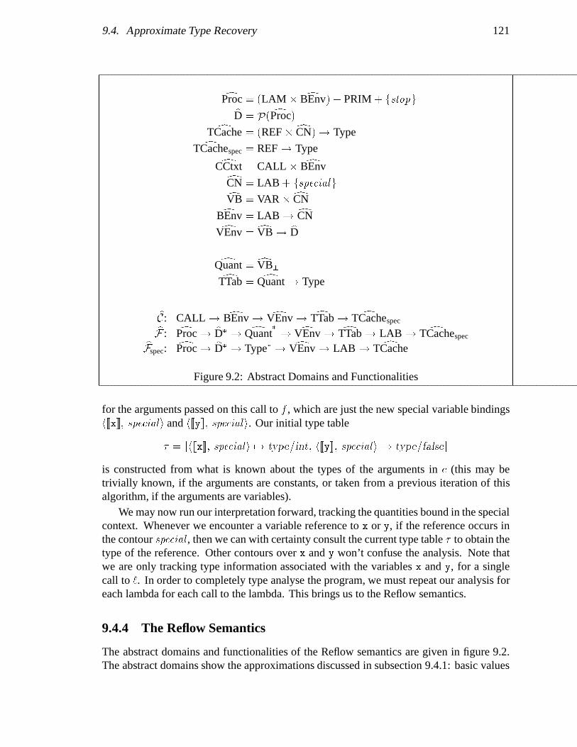
9.4. Approximate Type Recovery 121
dProc = (LAM � dBEnv) + PRIM + fstopgbD = P( dProc)
dTCache = (REF � dCN) ! TypedTCachespec = REF ! Type
dCCtxt = CALL � dBEnvdCN = LAB + fspecialgdVB = VAR �dCNdBEnv = LAB ! dCNdVEnv = dVB ! bD
dQuant = dVB?dTTab = dQuant ! Type
bC: CALL ! dBEnv ! dVEnv ! dTTab ! dTCachespecbF : dProc ! bD� ! dQuant�! dVEnv ! dTTab ! LAB ! dTCachespecbFspec: dProc ! bD� ! Type� ! dVEnv ! LAB ! dTCache
Figure 9.2: Abstract Domains and Functionalities
for the arguments passed on this call to f , which are just the new special variable bindingsh[[x]]; special i and h[[y]]; special i. Our initial type table
� =�h[[x]]; special i 7! type=int; h[[y]]; special i 7! type=false
�
is constructed from what is known about the types of the arguments in c (this may betrivially known, if the arguments are constants, or taken from a previous iteration of thisalgorithm, if the arguments are variables).
We may now run our interpretation forward, tracking the quantities bound in the specialcontext. Whenever we encounter a variable reference to x or y, if the reference occurs inthe contour special , then we can with certainty consult the current type table � to obtain thetype of the reference. Other contours over x and y won’t confuse the analysis. Note thatwe are only tracking type information associated with the variables x and y, for a singlecall to `. In order to completely type analyse the program, we must repeat our analysis foreach lambda for each call to the lambda. This brings us to the Reflow semantics.
9.4.4 The Reflow Semantics
The abstract domains and functionalities of the Reflow semantics are given in figure 9.2.The abstract domains show the approximations discussed in subsection 9.4.1: basic values

122 Chapter 9. Applications II: Type Recovery
have been dropped, the contour set dCN is finite, and elements of bD are sets of abstractprocedures, not single values. We’ll use the 1CFA abstraction, so the contours are call sitelabels plus the token special to mark the special reflow contour.
Notice that we have two different abstract variants of the F function: bF and bFspec.The bF function is the ordinary variant which allocates abstract contours when applyingprocedures. The bFspec function is the special variant which allocates the special contourwhen it is applied. The bFspec function is used only once per reflow, during the initial call.
The idea of the Reflow semantics is to track only one closure’s variables at a time. Thisis done by the Reflow function:
Reflow: dCCtxt ! dVEnv ! Type� ! dTCache:
For example, ReflowD[[(f a b)]]; b�E cve htype=int; type=proci restarts the program at
the call (f a b), in the context given by the abstract contour environment b� and variableenvironment cve , assuming a has type type=int and b has type type=proc. Reflow runs theprogram forward, tracking only the variables bound by the initial call to f, returning a typecache giving information about references to these variables. This is done by allocatinga single, special contour for the initial procedure called from (f a b), and tracking thevariables bound in this contour through an abstract execution of the program.
The initial type vector given to Reflow comes from an auxiliary function, TVInit:
TVInit: dCCtxt ! dTCache ! Type�
TVInitD[[(f a1 . . .an)]]; b�
E� = ht1; . . . ; tni
where ti = ai 2 REF �! �Dai;
b�(binder ai)E
otherwise At ai
TVInit takes a call context and a type cache, and returns the types of all the arguments inthe call. If the argument is a variable reference, the type cache is consulted; if the argumentis a constant or a lambda, the auxiliary functionAt gives the appropriate type.
If we wish to restart our program at an arbitrary call contextDc; b�E with Reflow, we
need a variable environment cve that approximates all the variable environments that everpertained at this call context. This is easy to handle: we always use the final variableenvironment that was present at the end of a control-flow analysis performed using thesingle-threaded environment algorithm of section 5.3. Since the variable environment isonly augmented monotonically during the course of this analysis, the terminal environmentis a superset of every intermediate variable environment through which the interpretationevolved. So, before performing the reflow analysis, we first perform a control-flow analysiswith the single-threaded environment algorithm. This produces two items critical for thereflow analysis: the call cache and terminal variable environment cve�nal . The domain ofthe call cache Dom( ) gives us the call contexts from which we must reflow, and cve�nalallows us to restart the interpretations in mid-stride.
Given TVInit and Reflow, we can construct a series of approximate type caches, con-verging to a fixed point. The initial type cache �0 is the most precise; at each iteration, we
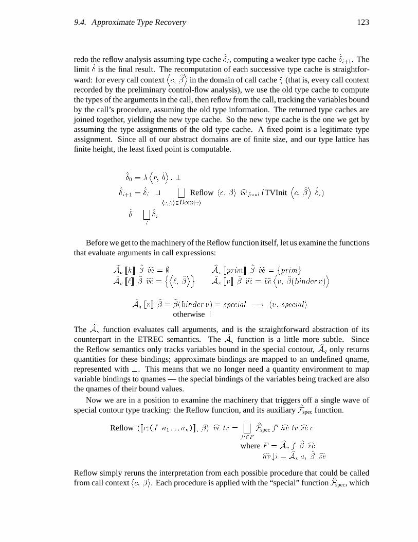
9.4. Approximate Type Recovery 123
redo the reflow analysis assuming type cache �i, computing a weaker type cache �i+1. Thelimit � is the final result. The recomputation of each successive type cache is straightfor-ward: for every call context
Dc; b�E in the domain of call cache (that is, every call context
recorded by the preliminary control-flow analysis), we use the old type cache to computethe types of the arguments in the call, then reflow from the call, tracking the variables boundby the call’s procedure, assuming the old type information. The returned type caches arejoined together, yielding the new type cache. So the new type cache is the one we get byassuming the type assignments of the old type cache. A fixed point is a legitimate typeassignment. Since all of our abstract domains are of finite size, and our type lattice hasfinite height, the least fixed point is computable.
�0 = �Dr; b
E: ?
�i+1 = �i tG
hc; �i2Dom( )
Reflow hc; �i cve�nal (TVInitDc; b�E �i)
� =Gi
�i
Before we get to the machinery of the Reflow function itself, let us examine the functionsthat evaluate arguments in call expressions:
bAv [[k]]b� cve = ; bAv [[prim]] b� cve = fprimg
bAv [[`]] b� cve =nD
`; b�Eo bAv [[v]] b� cve = cve Dv; b�(binder v)E
bAq [[v]]b� = b�(binder v) = special �! hv; special i
otherwise ?
The bAv function evaluates call arguments, and is the straightforward abstraction of itscounterpart in the ETREC semantics. The bAq function is a little more subtle. Sincethe Reflow semantics only tracks variables bound in the special contour, bAq only returnsquantities for these bindings; approximate bindings are mapped to an undefined qname,represented with ?. This means that we no longer need a quantity environment to mapvariable bindings to qnames — the special bindings of the variables being tracked are alsothe qnames of their bound values.
Now we are in a position to examine the machinery that triggers off a single wave ofspecial contour type tracking: the Reflow function, and its auxiliary bFspec function.
Reflow h[[c:(f a1 . . . an)]]; �i cve tv =G
f 02F
bFspec f0 cav tv cve c
where F = bAv fb� cve
cav#i = bAv ai b� cveReflow simply reruns the interpretation from each possible procedure that could be calledfrom call context hc; �i. Each procedure is applied with the “special” function bFspec, which

124 Chapter 9. Applications II: Type Recovery
arranges for the initial application of the procedure to be a special one. The 1CFA contourc passed to bFspec is the abstract contour that special will represent during this reflow. Thetype caches resulting from each call are joined together into the result cache.
The special application of a procedure performed by bFspec is done only at the beginningof the reflow. Instead of allocating the 1CFA contour b, bFspec allocates the special contourin its place, designating it the one and only special contour in a given execution thread.The incoming values are bound in the outgoing variable environment cve 0 under the specialcontour. The incoming type information is used to create the initial type table � passedforward to track the values bound under the special contour. The rest of the computation ishanded off to the bC procedure. bC is similar to C with the exception that it only records thetype information of references that are bound in the special contour.
bFspec
D[[`:(� (v1 . . . vn) c)]]; b�E cav tv cve b = despec b
� bC c b�0 cve 0 ��where � =
�hvi; special i 7! tv#i
�b�0
= b� �` 7! special�
cve 0 = cve t �hvi; special i 7! cav#i�
despec: CN ! dTCachespec ! dTCache
despec b �spec = �Dr; b0
E: b = b0 �! �spec r
otherwise ?
Because a single reflow tracks only the bindings of one special contour, the result typecache has information only for variable references bound in that contour. So the type cachereturned by the bC application indexes on variable references, not reference/contour pairs— the contour is understood to be the special contour. Now, for this particular reflow, thespecial contour allocated by bFspec stands for a particular abstract contour, b. So the resulttype cache must be converted to a type cache that replaces the simple variable reference r
entries withDr; b
Eentries. This is done with the auxiliary despec function. Let
� = despec b �spec :
Then �Dr; b
Ejust returns �spec r, and �
Dr; b0
Egives bottom when b0 6= b.
bFspec must also be defined over primops. Primops do not have variables to be tracked,so instead primops pass the buck to their continuations. The + primop uses its initial-typevector htx ; ty; tk i to compute the initial-type vector htsi for its continuation. The + primopthen employs bFspec to perform type recovery on the variable bound by its continuation.
bFspec [[p:+]]Dx; y; k
Ehtx ; ty; tk i cve b =
Gk2k
bFspec k h;i htsi cve icp
where ts = infer+htx ; tyi
The test-integer primop is even simpler. Since its continuations do not bind variables,there is nothing to track, so the function just immediately returns the bottom type cache.
bFspec [[test-integer]]Dx; k0; k1
Ehtx ; tk 0; tk 1i cve b = ?

9.4. Approximate Type Recovery 125
Once the initial call to bFspec has triggered a wave of type recovery for a particularlambda’s variables, the actual tracking of type information through the rest of the programexecution is handled by the bF and bC functions.
bC [[c:(f a1 . . . an)]] b� cve � = � t� Gf 02F
bF f 0 cav cqv cve � 0 c
�
where F = bAv fb� cve
cav#i = bAv aib� cve
[[ri:vi]] = ai (8ai 2 REF)[[r0:v0]] = f (if f 2 REF)bi =
b�(binder vi)qi =
bAq vib�
cqv = hq1=?; . . . ; qn=?i� =
�ri 7! � qi
�8qi 6= ?
� 0 = q0 6= ? �! � u>�q0 7! type=proc
�otherwise �
As bC evaluates its arguments, it checks to see if any are variables whose types are beingtracked. Suppose an argument ai is a variable reference [[ri:vi]]. The variable vi is beingtracked if it is bound in the special contour, that is, if bi = special , where bi =
b�(binder vi).In this case, it will be mapped to a non-bottom qname by bAq. If an argument is beingtracked, we look up its current type � qi, and record this in bC’s contribution � to the typecache. An outgoing type table � 0 is constructed, reflecting that f must be of type type/proc(again, note that this fact is only recorded in � 0 if f is a variable currently being tracked).The notation qi=? in the construction of the outgoing quantity vector cqv means “the valueof qi if it is defined, otherwise?.” In other words, if an argument ai is a variable reference,then the corresponding element in cqv is qi. If the argument is a lambda or constant, thenit clearly isn’t one of the special qnames created by bFspec at the beginning of the reflow,so the corresponding element in cqv is just ?. The rest of bC’s stucture is a straighforwardabstraction of the exact analysis. In keeping with the 1CFA abstraction, the call site c ispassed to bF to be used for its abstract contour.
Since multiple contours are identified together in the abstract semantics, values in theapproximate domain are sets of abstract procedures. Because of this, the call must branchto each of the possible procedures f 0 to which the expression f could evaluate. The resulttype caches are then all joined together.
An approximate, non-special contour is allocated when bF causes control to enter aclosure. Because multiple environments are thus identified together by bF applications, itcannot track type information for the variables bound by the procedure. Hence bF has afairly simple definition for the closure case, just augmenting the environment structure andpassing the closure’s body c off to bC.

126 Chapter 9. Applications II: Type Recovery
bFD[[`:(� (v1 . . . vn) c)]]; b�
Ecav cqv cve � b = bC c b�0 cve 0 �
where b�0 = b�h` 7! b
i
cve 0 = cve thDvi; b
E7! cav#i
i
bF ’s definition for the terminal stop continuation is, again, trivial, ignoring its argumentv and returning the bottom type cache:
bF [[stop]] cav cqv cve � b = ?:
bF ’s behavior on primops is more interesting. If the argument x is being tracked (i.e.,cqx is a quantity, not bottom), then we intersect type=int with cqx ’s incoming type, passingthe result type table �t to the true continuation, and we subtract type=int from cqx ’s type in�f the table passed to the false continuation. In other words, we do the type recovery of theETREC semantics, but only for the values being tracked.
bF [[p:test-integer]]Dx; k0; k1
E Dcqx ; cqk 0;
cqk 1
Ecve � b =
� G
k2^k0
bF k hi hi cve �t ic0p
�t
� G
k2^k1
bF k hi hi cve �f ic1p
�
where �f = cqx 6= ? �! ��cqx 7! (� cqx � type=int)
�
otherwise �
�t = cqx 6= ? �! ��cqx 7! (� cqx u type=int)
�
otherwise �
The + primop is similar. If the arguments x and y are being tracked, then we updatethe type table passed forward, otherwise we simply pass along the incoming type table� unchanged. Since the continuations k are applied by the approximate bF function, thequantity vector is h?i — we will not be tracking the variables bound by the call to k.
bF [[p:+]]Dx; y; k
E Dcqx ; cqy ; cqk
Ecve � b =
G
k2^k
bF k h;i h?i cve � 00 icp
where � 0 = cqx 6= ? �! ��cqx 7! (type=number u � cqx )�
otherwise �
� 00 = cqy 6= ? �! � 0�cqy 7! (type=number u � 0 cqy)�
otherwise � 0
To finish off the Reflow semantics, we must take care of letrec. Abstracting C’sdefinition for letrec is simple. Evaluating the letrec’s bound expressions only involvesclosing lambdas, not referencing variables. So the letrec will not “touch” any of thevariables we are currently tracking. Hence the letrecdoes not make any local contribution
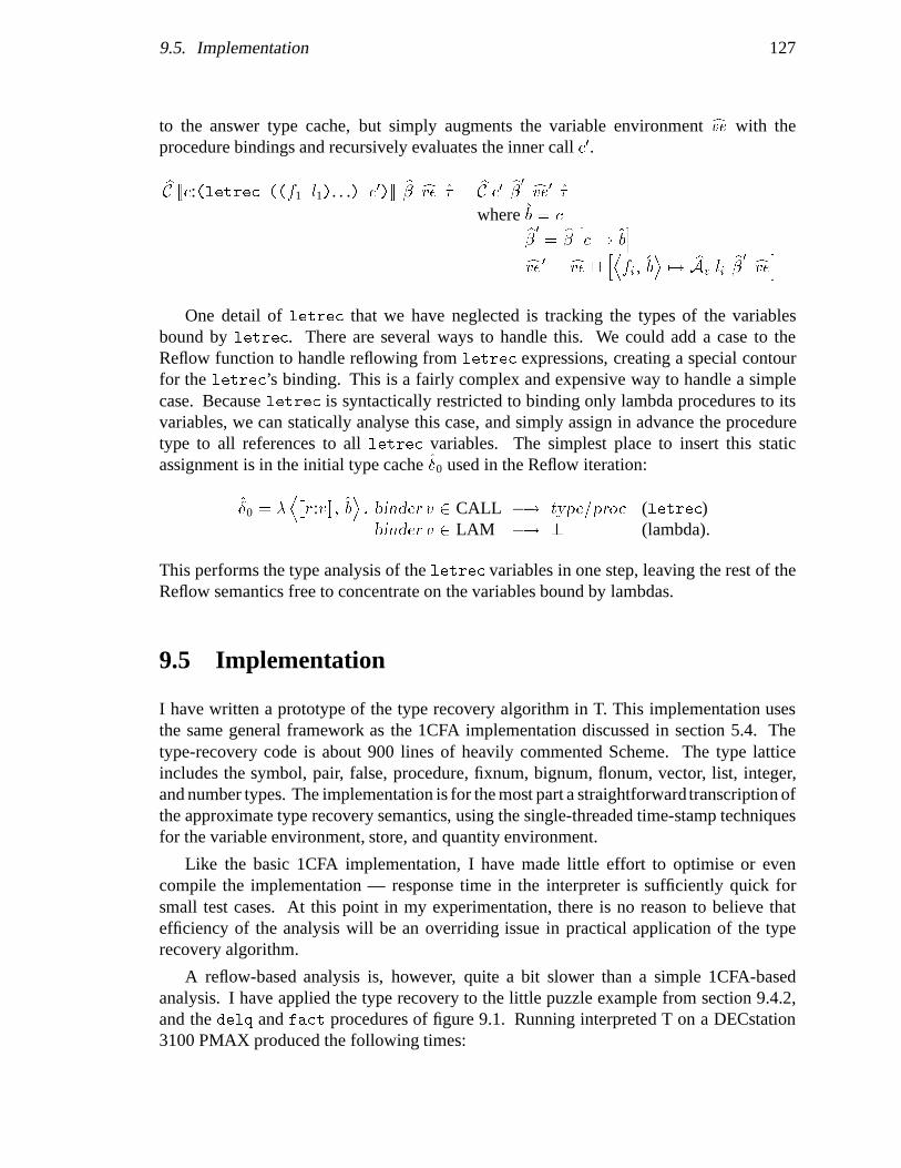
9.5. Implementation 127
to the answer type cache, but simply augments the variable environment cve with theprocedure bindings and recursively evaluates the inner call c0.
bC [[c:(letrec ((f1 l1). . .) c0)]] b� cve � = bC c0 b�0 cve 0 �where b = c
b�0 = b�hc 7! b
i
cve 0 = cve thDfi; b
E7! bAv li
b�0 cvei
One detail of letrec that we have neglected is tracking the types of the variablesbound by letrec. There are several ways to handle this. We could add a case to theReflow function to handle reflowing from letrec expressions, creating a special contourfor the letrec’s binding. This is a fairly complex and expensive way to handle a simplecase. Because letrec is syntactically restricted to binding only lambda procedures to itsvariables, we can statically analyse this case, and simply assign in advance the proceduretype to all references to all letrec variables. The simplest place to insert this staticassignment is in the initial type cache �0 used in the Reflow iteration:
�0 = �D[[r:v]]; b
E: binder v 2 CALL �! type=proc (letrec)binder v 2 LAM �! ? (lambda).
This performs the type analysis of the letrec variables in one step, leaving the rest of theReflow semantics free to concentrate on the variables bound by lambdas.
9.5 Implementation
I have written a prototype of the type recovery algorithm in T. This implementation usesthe same general framework as the 1CFA implementation discussed in section 5.4. Thetype-recovery code is about 900 lines of heavily commented Scheme. The type latticeincludes the symbol, pair, false, procedure, fixnum, bignum, flonum, vector, list, integer,and number types. The implementation is for the most part a straightforward transcription ofthe approximate type recovery semantics, using the single-threaded time-stamp techniquesfor the variable environment, store, and quantity environment.
Like the basic 1CFA implementation, I have made little effort to optimise or evencompile the implementation — response time in the interpreter is sufficiently quick forsmall test cases. At this point in my experimentation, there is no reason to believe thatefficiency of the analysis will be an overriding issue in practical application of the typerecovery algorithm.
A reflow-based analysis is, however, quite a bit slower than a simple 1CFA-basedanalysis. I have applied the type recovery to the little puzzle example from section 9.4.2,and the delq and fact procedures of figure 9.1. Running interpreted T on a DECstation3100 PMAX produced the following times:

128 Chapter 9. Applications II: Type Recovery
puzzle 5.1 secfact 7.8 secdelq 5.3 sec
As an example of the algorithm’s power, it is able to completely recover the types ofall variable references in the delq and fact procedures given in section 9.1. The typesrecovered for the puzzle and fact examples are shown in detail in appendix B.
The allure of type recovery, of course, is type-safe Scheme implementations with littlerun-time overhead. It remains to be seen whether there is enough recoverable type infor-mation in typical code to allow extensive optimisation. The algorithm has not been testedextensively on a large body of real code. However, these early results are encouraging.
9.6 Discussion and Speculation
This section is a collection of small discussions and speculations on various aspects ofScheme type recovery.
9.6.1 Limits of the Type System
From the optimising compiler’s point of view, the biggest piece of bad news in the Schemetype system is the presence of arbitrary-precision integers, or “bignums.” Scheme’sbignums, an elegant convenience from the programmer’s perspective, radically interferewith the ability of type recovery to assign small integer “fixnum” types to variable refer-ences. The unfortunate fact is that two’s complement fixnums are not closed under anyof the common arithmetic operations. Clearly adding, subtracting, and multiplying twofixnums can overflow into a bignum. Less obvious is that simple negation can overflow:the most negative fixnum overflows when negated. Because of this, not even fixnum di-vision is safe: dividing the most negative fixnum by �1 negates it, causing overflow intobignums. Thus, the basic fixnum arithmetic operations cannot be safely implemented withtheir corresponding simple machine operations. This means that most integer quantitiescannot be inferred to be fixnums. So, even though type recovery can guarantee that all thegeneric arithmetic operations in figure 9.1’s factorial function are integer operations, thisdoes not buy us a great deal.
Not being able to efficiently implement safe arithmetic operations on fixnums is terriblenews for loops, because many loops iterate over integers, particularly array-processingloops. Taking five instructions just to increment a loop counter can drastically affect theexecution time of a tight inner loop.
There are a few approaches to this problem:
� Range analysisRange analysis is a data-flow analysis technique that bounds the values of numeric

9.6. Discussion and Speculation 129
variables [Harrison 77]. For example, range analysis can tell us that in the body ofthe following C loop, the value of i must always lie in the range [0; 10):
for(i=9; i>=0; i--) printf("%d ", a[i]);
Range analysis can probably be applied to most integer loop counters. Consider thestrindex procedure below:
(define (strindex c str)
(let ((len (string-length str)))
(letrec ((lp (lambda (i)
(cond ((>= i len) -1) ; lose
((char= c (string-ref str i)) i) ; win
(else (loop (+ i 1))))))) ; loop
(lp 0))))
Type recovery can guarantee that len, being the result of the string-lengthprimop,is a fixnum. Range analysis can show that i is bounded by 0 and a fixnum; this isenough information to guarantee that i is a fixnum. Range analysis is useful in itsown right as well — in this example, it allows us to safely open-code the characteraccess (string-ref str i) with no bounds check.
� Abstract safe usage patternsThe poor man’s alternative to range analysis is to take the usage patterns that areguaranteed to be fixnum specific, and package them up for the user as syntactic orprocedural abstractions. These abstractions can be carefully decorated withproclaimdeclarations to force fixnum arithmetic. For example, a loop macro which has a(for c in-string str) clause can safely declare the string’s index variable as afixnum. This approach can certainly pick up string and array index variables.
� Disable bignumsAnother cheap alternative to range analysis is to live dangerously and provide acompiler switch or declaration which allows the compiler to forget about bignums andassume all integers are fixnums. Throwing out bignums allows simple type recoveryto proceed famously, and programs can be successfully optimised (successfully, thatis, until some hapless user’s program overflows a fixnum. . . ).
� Hardware supportSpecial tag-checking hardware, such as is provided on the SPARC, Spur and LispMachine architectures [Garner+ 88, Hill+ 86, Moon 85], or fine-grained parallelism,such as is provided by VLIW architectures [Ellis 86, Fisher+ 84], allow fixnumarithmetic to be performed in parallel with the bignum/fixnum tag checking. In thiscase, the limitations of simple type recovery are ameliorated by hardware assistance.
VLIW’s could be ideal target machines for languages that require run-time type-checking. For example, when compiling the code for a safe car application, thecompiler can pick the trace through the type test that assumes the car’s argument
130 Chapter 9. Applications II: Type Recovery
is a legitimate pair. This will almost always be correct, the sort of frequency skewthat allows trace scheduling to pay off in VLIW’s. The actual type check operationcan percolate down in the main trace to a convenient point where ALU and branchresources are available; the error-handling code is off the main trace.
Common cases for generic arithmetic operations are similarly amenable to tracepicking. The compiler can compile a main fixnum trace (or flonum trace, as thecommon case may be), handling less frequent cases off-trace. The overhead forbignum, rational, and complex arithmetic ops will dominate the off-trace time inany event, whereas the lightweight fixnum or flonum case will be inlined. This ideacan also be extended to other sorts of lightweight traps that higher-order languagestypically require, such as bounds checking for inlined heap allocation.
The VLIW trace-scheduling approach to run-time type safety has an interestingcomparison to the automatic tag checking performed by Lisp Machines. Essentially,we have taken the tag-checking ALU and branch/trap logic, promoted it to general-purpose status, and exposed it to the compiler. These hardware resources can now beused for non-typechecking purposes when they would otherwise lay idle, providingopportunities for increased fine-grained parallelism.
The Lisp Machine approach is the smart hardware/fast compiler approach; the VLIWapproach is the other way ’round.
9.6.2 Declarations
The dangerous proclaim declaration is problematic. A purist who wants to provide aguaranteed safe Scheme implementation might wish to ban proclaim on the grounds thatit allows the user to write dangerous code. A single address-space, personal computerimplementation of Scheme, for example, might rely on run-time safety to prevent threadsfrom damaging each other’s data. Including proclaim would allow the compilation ofcode that could silently trash the system, or access and modify another thread’s data.
On the other hand, safe declarations like enforce have limits. Some useful datatypescannot be checked at run time. For example, while it is possible to test at run time if a datumis a procedure, it is not possible, in general, to test at run time if a datum is a procedure thatmaps floating-point numbers to floating-point numbers. Allowing the user to make sucha declaration can speed up some critical inner loops. Consider the floating-point numericintegrator below:
(define (integ f x0 x1 n)
(enforce procedure? f) (enforce fixnum? n)
(enforce flonum? x0) (enforce flonum? x1)
(let ((delta (/ (- x1 x0) n)))
(do ((i n (- i 1))
(x x0 (+ x delta))
(sum 0.0 (+ sum (f x))))
((= i 0) (* sum delta)))))

9.6. Discussion and Speculation 131
In some cases, an analysis might be able to find all applications of the integrator, and thusdiscover that f is always bound to a floating-point function. However, if the integratoris a top level procedure in an open system, we can’t guarantee at compile time that fis a floating-point function, and we can’t check it at run time. This means that the sumoperation must check the return value of f each time through the loop to ensure it is alegitimate floating-point value.
While the proclaim declaration does allow the user to write dangerous code, it is atleast a reasonably principled loophole. Proclaim red-flags dangerous assumptions. If theuser can be guaranteed that only code marked with proclaim declarations can behave inundefined ways, debugging broken programs becomes much easier.
Finally, it might be worth considering a third declaration, probably. The declaration(probably flonum? x) is a hint to the compiler that x is most likely a floating-point value,but could in fact be any type. Having a probably declaration can allow trace-schedulingcompilers to pick good traces or optimistically open-code common cases.
9.6.3 Test Hoisting
Having one branch of a conditional test be the undefined effect $ or error primop opens upinteresting code motion possibilities. Let us call tests with an (error) arm “error tests,”and tests with a ($) arm “$-tests.” These tests can be hoisted to earlier points in the codethat are guaranteed to lead to the test. For example,
(block (print (+ x 3))
(if (fixnum? x) (g x) ($)))
can be legitimately transformed to
(if (fixnum? x) (block (print (+ x 3)) (g x))
($))
because the compiler can choose any effect it likes for the undefined effect operator,including the effect of (print (+ x 3)). This can be useful, because hoisting type testsincreases their coverage. In the example above, hoisting the fixnum? test allows thecompiler to assume that x is a fixnum in the (+ x 3) code.
Further, error and $-tests can be hoisted above code splits if the test is applied in botharms. For example, the type tests in
(if (> x 0)
(if (pair? y) (bar) ($))
(if (pair? y) (baz) ($)))
can be hoisted to a single type test:
(if (pair? y)
(if (> x 0) (bar) (baz))
($))

132 Chapter 9. Applications II: Type Recovery
Real savings accrue if loop invariant type tests get hoisted out of loops. For example,in a naive, declaration-free dot-product subroutine,
(define (dot-prod v w len)
(do ((i (- len 1) (- i 1))
(sum 0.0 (+ sum (* (vector-ref v i) (vector-ref w i)))))
((< i 0) sum)))
each time through the inner loop we must check that v and w have type vector. Since v
and w are loop invariants, we could hoist the run-time type checks out of the loop, whichwould speed it up considerably. (In this particular example, we would have to duplicatethe termination test (< i 0), so that loop invariant code pulled out of the loop would onlyexecute if the loop was guaranteed at least one iteration. This is a standard optimisingcompiler technique.)
Hoisting error tests requires us to broaden our semantics to allow for early detectionof run-time errors. If execution from a particular control point is guaranteed to lead to asubsequent error test, it must be allowed to perform the error test at the control point instead.
In the general case, error and $-test hoisting is a variant of very-busy expression analysis[Aho+ 86]. Note that hoisting$-tests gives a similar effect to the backwards type inferencingof Kaplan and Ullman [Kaplan+ 80]. Finding algorithms to perform this hoisting is an openresearch problem.
Note that the sort of “dangerous” compilation permitted by the undefined effect, and itsformal description via the ($) operator is of dubious semantic merit. However, implemen-tors persist in making dangerous implementations, so program analyses need to supportthem.
9.6.4 Other Applications
The general approach to solving quantity-based analyses presented in this chapter can beapplied to other data-flow problems in higher-order languages. The range analysis discussedin subsection 9.6.1 is a possible candidate for this type of analysis.
One analysis very similar to type recovery is future analysis. Some parallel dialectsof Scheme [Kranz+ 89] provide futures, a mechanism for introducing parallelism into aprogram. When the form (future <exp>) is evaluated, a task is spawned to evaluate theexpression <exp>. The future form itself immediately returns a special value, called afuture. This future can be passed around the program, and stored into and retrieved fromdata structures until its actual value is finally required by a “strict” operator such as + or car.If the future’s task has completed before the value is needed, the strict operation proceedswithout delay; if not, the strict operator must wait for the future’s task to run to completionand return a value.
Futures have a heavy implementation expense on conventional hardware, because allstrict operators must check their operands. Future checking can add a 100% overhead tothe serial run time of an algorithm on conventional hardware.

9.7. Related Work 133
“Future analysis” is simply realising that after a variable has been used as an argumentto a strict operator, it’s value is guaranteed to be a non-future. So following references tothe variable don’t have to perform the future check. Thus, in the lambda
(� (x) (print (car x)) . . . (f (cdr x)) . . . )
the (cdr x) operation can be compiled without future checking. Clearly, this is identicalto the type-recovery analysis presented in this chapter, and the same techniques apply.
9.7 Related Work
Steenkiste’s dissertation [Steenkiste 87] gives some idea of the potential gains type recoverycan provide. For his thesis, Steenkiste ported the PSL LISP compiler to the Stanford MIPS-Xprocessor. He implemented two backends for the compiler. The “careful” backend did fullrun-time type checking on all primitive operations, including car’s, cdr’s, vector references,and arithmetic operations. The “reckless” backend did no run-time type checking at all.Steenkiste compiled about 11,500 lines of LISP code with the two backends, and comparedthe run times of the resulting executables. Full type checking added about 25% to theexecution time of the program.
Clearly, the code produced by a careful backend optimised with type-recovery analysiswill run somewhere between the two extremes measured by Steenkiste. This indicates thatthe payoff of compile-time optimisation is bounded by the 25% that Steenkiste measured.Steenkiste’s data, however, must be taken only as a rough indicator. In LISP systems, the tinydetails of processor architecture, compiler technology, data representations and programapplication all interact in strong ways to affect final measurements. Some examples of theparticulars affecting his measurements are: his LISP system used high bits for type tags;the MIPS-X did not allow car and cdr operations to use aligned-address exceptions todetect type errors; his 25% measurement did not include time spent in the type dispatchof generic arithmetic operations; his generic arithmetic was tuned for the small integercase; none of his benchmarks were floating-point intensive applications; his measurementsassumed interprocedural register allocation, a powerful compiler technology still not yet incommon practice in LISP and Scheme implementations; and LISP requires procedural datato be called with the funcall primop, so simple calls can be checked at link time to ensurethey are to legitimate procedures.
These particulars of language, hardware architecture, implementation, and program canbias Steenkiste’s 25% in both directions. Steenkiste gives a careful description of most ofthese issues. However, even taken as a rough measurement, Steenkiste’s data do indicatethat unoptimised type-checking is a significant component of program execution time, andthat there is room for compile-time optimisation to provide real speed-up.
The idea of type recovery for Scheme is not new. Vegdahl and Pleban [Vegdahl+ 89]discuss the possibility of “tracking” types through conditionals, although this was neverpursued. The ORBIT compiler is able to track the information determined by conditional

134 Chapter 9. Applications II: Type Recovery
branches, thus eliminating redundant tests. ORBIT, however, can only recover this infor-mation over trees of conditional tests; more complex control and environment structures,such as loops, recursions, and joins block the analysis.
Curtis discusses a framework for performing static type inference in a Scheme vari-ant [Curtis 90], along the lines of that done for statically typed polymorphic languagessuch as ML [Milner 85] or LEAP [Pfenning+ 90]. However, his work assumes that most“reasonable” Scheme programs use variables in a way that is consistent with a static typingdiscipline. In essence, Curtis’ technique types variables, whereas the analysis developedin this chapter types variable references, an important distinction for Scheme. Note thatwithout introducing type-conditional primitives that bind variables, and (perhaps automat-ically) rewriting Scheme code to employ these primitives, this approach cannot recover theinformation determined by conditional branches on type tests, an important source of typeinformation.
Traditional data-flow analysis techniques have also been used to perform type re-covery for latently-typed variants of traditional imperative languages [Tenenbaum 74,Kaplan+ 80][Aho+ 86, chapter 10]. These approaches differ from the technique devel-oped in this chapter in the following ways:
� First, they focus on side-effects as the principal way values are associated withvariables. In Scheme, variable binding is the predominant mechanism for associatingvalues with variables, so the Scheme type recovery analysis must focus on variablebinding.
� Second, they assume a fixed control-flow graph. Higher-order languages require thecontrol-flow analysis technology developed in this dissertation.
� Third, they assume a single, flat environment. Scheme forces one to consider multiplebindings of the same variable. The reflow semantics of section 9.4 correctly handlesthis complexity.
� Finally, they are not semantically based. The type recovery analysis in this chapteris based on the method of non-standard abstract semantic interpretations. Thisestablishes a formal connection between the analysis and the base language semantics.Grounding the analysis in denotational semantics allows the possibility of provingvarious useful properties of the analysis.
These differences are all connected by the centrality of lambda in Scheme. The prevalenceof lambda is what causes the high frequency of variable binding. Lambda allows theconstruction of procedural data, which in turn prevent the straightforward construction of acompile-time control-flow graph. Lambda allows closures to be constructed, which in turnprovide for multiple extant bindings of the same variable. And, of course, the mathematicalsimplicity and power of lambda makes it much easier to construct semantically-basedprogram analyses.
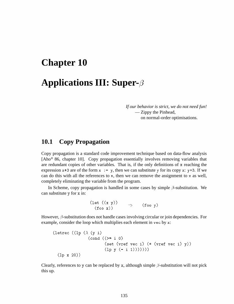
Chapter 10
Applications III: Super-�
If our behavior is strict, we do not need fun!— Zippy the Pinhead,
on normal-order optimisations.
10.1 Copy Propagation
Copy propagation is a standard code improvement technique based on data-flow analysis[Aho+ 86, chapter 10]. Copy propagation essentially involves removing variables thatare redundant copies of other variables. That is, if the only definitions of x reaching theexpression x+3 are of the form x := y, then we can substitute y for its copy x: y+3. If wecan do this with all the references to x, then we can remove the assignment to x as well,completely eliminating the variable from the program.
In Scheme, copy propagation is handled in some cases by simple �-substitution. Wecan substitute y for x in:
(let ((x y))
(foo x))) (foo y)
However, �-substitution does not handle cases involving circular or join dependencies. Forexample, consider the loop which multiplies each element in vec by x:
(letrec ((lp (� (y i)
(cond ((>= i 0)
(set (vref vec i) (* (vref vec i) y))
(lp y (- i 1)))))))
(lp x 20))
Clearly, references to y can be replaced by x, although simple �-substitution will not pickthis up.
135

136 Chapter 10. Applications III: Super-�
Note that this sort of copy propagation can frequently and usefully be applied to thecontinuation variable in the CPS expansions of loops. An example is the summation loopfrom the end of chapter 3. Partially CPS-converted, that loop looks like this:
(� (n k)
(letrec ((lp (� (i sum c)
(if (zero? i) (c sum)
(lp (- i 1) (+ sum i) c)))))
(lp n 0 k)))
The loop’s continuation c is always bound to the procedure’s continuation k, and is re-dundantly passed around the loop until it is invoked on loop termination. Applying copypropagation (and one round of useless-variable elimination to clean up afterwards) removesthe iteration variable c entirely:
(� (n k)
(letrec ((lp (� (i sum)
(if (zero? i) (k sum)
(lp (- i 1) (+ sum i))))))
(lp n 0)))
This sort of situation crops up frequently in CPS-expanded loops.
The general form of Scheme copy propagation, then, is:
For a given variable v, find all lexically inferior variables that are always boundto the value of v, and replace their references with references to v.
A variable is lexically inferior to v if its binding lambda occurs within the scope of v’sbinding lambda. With this definition, Scheme copy propagation acts as a sort of “super-�”substitution rule. (If we allow side-effects to variables, this can disallow some possiblesubstitutions. If, on the other hand, we use an intermediate representation that has novariable side-effects, we can substitute at will. This is one of the attractions of removingvariable assignments from the intermediate representation with assignment conversion. MLelegantly avoids the issue by disallowing assignments to variables altogether.)
Note that the environment problemrears its head here. For example, we cannot substitutex for y in the following code:
(let ((f (� (x h) (if (null? h) (� () x)
(let ((y (h))) . . . y . . . )))))(f 3 (f 5 nil)))
Even though y is certainly bound to x (because h is bound to (� () x) at that point), it’sthe wrong binding of x — we need the one that is in the y reference’s context. We havemultiple bindings of the same variable around at the same time, and so we have to be carefulwhen we are doing copy propagation to keep these multiple environments separate.

10.2. Lambda Propagation 137
10.1.1 Copy Propagation and Reflow Analysis
We can use reflow analysis to handle the environment problem raised by copy propagation.
Suppose we have some lambda ` = (� (x y z) . . .), and we wish to perform copypropagation on x. That is, we want to find the lexically inferior variables that are alwaysbound to the (lexically apparent) value of x so we can replace them with x. We do a reflow,starting with each entry to `. As we enter `, we create a special contour for `’s variables.All the lexically inferior lambdas in this scope will be closed over `’s special contour, andso won’t get their references to x confused with other bindings of x.
In order to perform the analysis, we need an abstract value domain of two values: avalue to represent whatever is bound to the binding of x that we’re tracking, and a value torepresent everything else in the system. Call x’s value 0 and the other value 1. The initialsystem state when we begin a reflow by entering ` is that
� the current binding of x has value 0
� all other bindings in the environment — including the current bindings of y and z
and other extant bindings of x — and all values in the abstract store have value 1.
As we proceed through the abstract interpretation, whenever we enter a lambda `0 thatis lexically inferior to `, we check to see if `0 is closed over the special ` contour we’retracking. If it is, we save away the value sets passed in as arguments to the variables of `0.
After we’ve reflowed ` from all of its call sites, we examine each lexically inferiorvariable. Consider the value set accumulated for variable v. If it is ;, then v’s lambda wasnever called — it’s dead code. If it is f0g, then it is always bound to the value of x in itslexical context, and so is a candidate for copy propagation — we can legitimately replaceall references to v with x. If it is f0;1g or f1g, then it can potentially be bound to anothervalue, and so is not a candidate for copy propagation.
Notice the conservative nature of the analysis: the presence of 1 in a value set marksa variable as a non-copy. This is because after setting up the initial special contour, allthe other variable bindings to value sets happen in approximate contours. This means thatdifferent bindings can get mapped together. If our analysis arranges for this to affect theanalysis in the safe direction, this identification is OK. Ruling out a possible copy is erringon the safe side, and that is the effect we get by unioning together the value sets and lookingfor 1’s .
10.2 Lambda Propagation
In the CPS Scheme intermediate representation, a call argument can be a variable, a constant,or a lambda. Constant propagation (from section 7.3) and copy propagation are essentiallyjust finding out when a variable is bound to a known variable or constant, and doing theappropriate substitution. Clearly there’s one important case left to be done: binding avariable to a known lambda, which we can call “lambda propagation.”
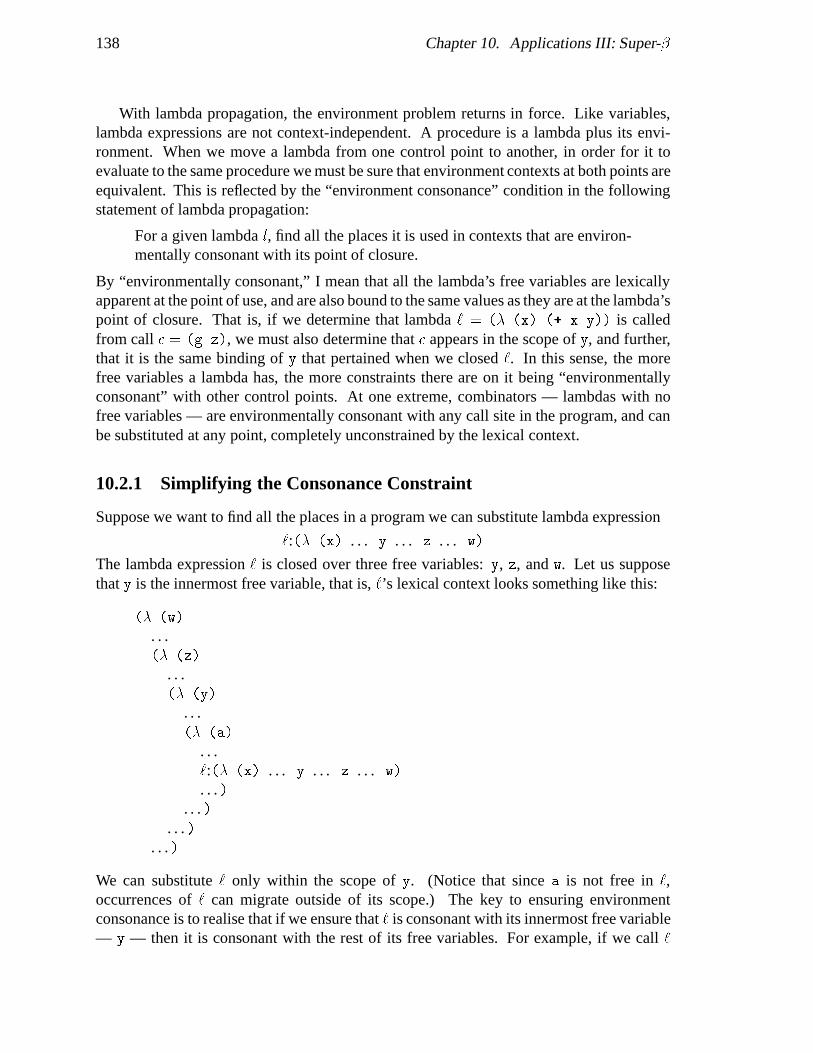
138 Chapter 10. Applications III: Super-�
With lambda propagation, the environment problem returns in force. Like variables,lambda expressions are not context-independent. A procedure is a lambda plus its envi-ronment. When we move a lambda from one control point to another, in order for it toevaluate to the same procedure we must be sure that environment contexts at both points areequivalent. This is reflected by the “environment consonance” condition in the followingstatement of lambda propagation:
For a given lambda l, find all the places it is used in contexts that are environ-mentally consonant with its point of closure.
By “environmentally consonant,” I mean that all the lambda’s free variables are lexicallyapparent at the point of use, and are also bound to the same values as they are at the lambda’spoint of closure. That is, if we determine that lambda ` = (� (x) (+ x y)) is calledfrom call c = (g z), we must also determine that c appears in the scope of y, and further,that it is the same binding of y that pertained when we closed `. In this sense, the morefree variables a lambda has, the more constraints there are on it being “environmentallyconsonant” with other control points. At one extreme, combinators — lambdas with nofree variables — are environmentally consonant with any call site in the program, and canbe substituted at any point, completely unconstrained by the lexical context.
10.2.1 Simplifying the Consonance Constraint
Suppose we want to find all the places in a program we can substitute lambda expression
`:(� (x) . . . y . . . z . . . w)
The lambda expression ` is closed over three free variables: y, z, and w. Let us supposethat y is the innermost free variable, that is, `’s lexical context looks something like this:
(� (w)
. . .(� (z)
. . .(� (y)
. . .(� (a)
. . .`:(� (x) . . . y . . . z . . . w)
. . .). . . )
. . . ). . .)
We can substitute ` only within the scope of y. (Notice that since a is not free in `,occurrences of ` can migrate outside of its scope.) The key to ensuring environmentconsonance is to realise that if we ensure that ` is consonant with its innermost free variable— y — then it is consonant with the rest of its free variables. For example, if we call `
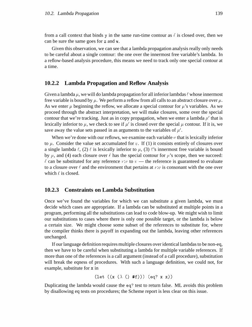
10.2. Lambda Propagation 139
from a call context that binds y in the same run-time contour as ` is closed over, then wecan be sure the same goes for z and w.
Given this observation, we can see that a lambda propagation analysis really only needsto be careful about a single contour: the one over the innermost free variable’s lambda. Ina reflow-based analysis procedure, this means we need to track only one special contour ata time.
10.2.2 Lambda Propagation and Reflow Analysis
Given a lambda�, we will do lambda propagation for all inferior lambdas `whose innermostfree variable is bound by �. We perform a reflow from all calls to an abstract closure over�.As we enter � beginning the reflow, we allocate a special contour for �’s variables. As weproceed through the abstract interpretation, we will make closures, some over the specialcontour that we’re tracking. Just as in copy propagation, when we enter a lambda �0 that islexically inferior to �, we check to see if �0 is closed over the special � contour. If it is, wesave away the value sets passed in as arguments to the variables of �0.
When we’re done with our reflows, we examine each variable v that is lexically inferiorto �. Consider the value set accumulated for v. If (1) it consists entirely of closures overa single lambda `, (2) ` is lexically inferior to �, (3) `’s innermost free variable is boundby �, and (4) each closure over ` has the special contour for �’s scope, then we succeed:` can be substituted for any reference r:v to v — the reference is guaranteed to evaluateto a closure over ` and the environment that pertains at r:v is consonant with the one overwhich ` is closed.
10.2.3 Constraints on Lambda Substitution
Once we’ve found the variables for which we can substitute a given lambda, we mustdecide which cases are appropriate. If a lambda can be substituted at multiple points in aprogram, performing all the substitutions can lead to code blow-up. We might wish to limitour substitutions to cases where there is only one possible target, or the lambda is belowa certain size. We might choose some subset of the references to substitute for, wherethe compiler thinks there is payoff in expanding out the lambda, leaving other referencesunchanged.
If our language definition requires multiple closures over identical lambdas to be non-eq,then we have to be careful when substituting a lambda for multiple variable references. Ifmore than one of the references is a call argument (instead of a call procedure), substitutionwill break the eqness of procedures. With such a language definition, we could not, forexample, substitute for x in
(let ((x (� () #f))) (eq? x x))
Duplicating the lambda would cause the eq? test to return false. ML avoids this problemby disallowing eq tests on procedures; the Scheme report is less clear on this issue.
140 Chapter 10. Applications III: Super-�
One case definitely worth treating with caution is when a lambda is used in its ownbody, e.g.:
(letrec ((fact (� (n)
(if (= n 0) 1
(* n (fact (- n 1)))))))
(fact m))
Lambda propagation tells us we can legitimately substitute the lambda definition of factfor the variable reference fact in its own body, giving us (after one round of substitution):
(letrec ((fact (� (n)
(if (= n 0) 1
(* n ((� (n) (if (= n 0) 1
(* n (fact (- n 1)))))
(- n 1)))))))
(fact m))
Clearly, blindly performing this substitution can get us into an infinite regress. This sort ofsituation can happen without letrec, in cases involving self-application
(let ((lp0 (� (lp1) (lp1 lp1)))) (lp0 lp0))
or indirection through the store:
(let* ((pair (cons #f #f))
(lp (� () ((car pair)))))
(set-car! pair lp)
(lp))
Substituting a lambda for a variable inside the lambda’s body is not necessarily a bad thingto do. It is a generalisation of loop unrolling, which can be desirable in some contexts. Butthe code optimiser must be aware of this case, and avoid it when it is undesirable.
Most of these substitution constraints also pertain to code improvers that use simple�-substitution; detailed discussions are found in the Rabbit, Orbit and TransformationalCompiler theses [Steele 78, Kranz+ 86, Kelsey 89]. Note that with the exception of proce-dural eqness, these caveats are all issues of implementation, not semantics (code blow-up isnot, for example, a semantic concern). This casts some suspicion on the procedural eqnessrequirement.
A final note on lambda propagation. As we’ve just seen, there are many constraintsdetermining when we can substitute a lambda for a variable known to be bound to a closureover that lambda: the variable’s reference context must be environmentally consonant withthe lambda’s point of closure; the variable must be referenced only once (to avoid codeblow-up); and so forth. However, even when these constraints are not satisfied, it is usefulto know that a variable reference must evaluate to a closure over a particular lambda. Thecompiler can compile a procedure call as a simple branch to a known location instead of a
10.3. Cleaning Up 141
jump to a run-time value which must be loaded into a register. If all calls to a lambda areknown calls, the compiler can factor the lambda out of the run-time representation of theclosure, allowing for smaller, more efficient representations. This is exactly what Orbit’sstrategy analysis does, for the simple cases it can spot.
10.3 Cleaning Up
When we substitute an expression — a variable, a constant or a lambda — for all referencesto some variable v, then v becomes a useless variable. It is therefore a candidate forbeing removed from its lambda’s parameter list. This transformation is the one used bythe second phase of useless-variable elimination (section 7.2). The following sequence oftransformations shows the role of UVE in post-substitution cleanup.
;;; Original loop
(letrec ((lp (� (sum n c)
(if (= 0 n) (c sum)
(lp (+ sum n) (- n 1) c)))))
(lp 0 m k))
;;; After copy propagation
(letrec ((lp (� (sum n c)
(if (= n 0) (k sum)
(lp (+ sum n) (- n 1) k)))))
(lp 0 m k))
;;; After UVE
(letrec ((lp (� (sum n)
(if (= n 0) (k sum)
(lp (+ sum n) (- n 1))))))
(lp 0 m))
10.4 A Unified View
Copy and constant propagationare classical code improvements based on data-flow analysis.Standard imperative languages typically use side-effects to associate variables with values,and this is what the standard formulations of copy and constant propagation focus on. InScheme, however, variables are typically associated with values by binding them. Withthis change of emphasis, copy and constant propagation become simply special cases ofan interesting generalisation of the �-calculus �-substitution rule. This is particularly truein the CPS Scheme internal representation, where side-effects are not allowed to interferewith the substitution rules. This “super-�” model of code improvement gives us one more
142 Chapter 10. Applications III: Super-�
alternative to copy and constant propagation: “lambda propagation” — substituting lambdaexpressions for variable references.
At this point, we can see that constant, copy and lambda propagation are actually threefacets of the same basic problem: substituting known expressions for the variables boundto them in the CPS intermediate representation.
In the case of copy and lambda propagation, the context-dependence of variable ref-erences and lambda expressions requires our analysis to be sensitive to the environmentthat exists at the source and target points of the expression being substituted. This is theenvironment problem introduced in chapter 8; its solution is based on the general techniqueof reflow analysis.
Chapter 11
Future Work
Dissertations are not finished;they are abandoned.
— H. Q. Bovik
The research I’ve reported on in this dissertation opens up many possible avenues for futurework. In this chapter, I will sketch what I think are some of the more interesting ones.
11.1 Theory
Classical research in optimising compilers has had little use for formal semantics. The greatallure of non-standard abstract semantic interpretation is that it can bridge these two areas. Itprovides a framework for compile-time analysis that is grounded in denotational semantics.This raises the possibility of proving that the optimising transformations implemented bya compiler are denotationally invariant: mathematically showing they leave the meaningof a program unchanged. Anyone who has ever been tripped up by a buggy optimisingcompiler will recognise the attraction of a formally verified optimiser.
Pleban’s dissertation [Pleban 81] clearly sets forth the NSAS manifesto: to unify thefields of language semantics and compile-time program analysis under the formalismsof denotational semantics. Although concerned specifically with the problem of storageanalysis (“compile-time garbage collection”), Pleban calls for a comprehensive programto express the corpus of traditional compiler optimisation techniques in terms of languagesemantics. His dissertation does not, however, deliver on this vision.
Neither does mine. The mathematics in this dissertation is concerned mainly withthe foundations of control-flow analysis. I have not done any theoretical work on theoptimisations that are based on control-flow analysis. It is still an open problem to show,for example, that the induction-variable elimination analysis and transformation of chapter7 preserves the meaning of the program. In the applications chapters (7, 9, and 10), I haverelied on the reader’s intuition and informal arguments of correctness.
143
144 Chapter 11. Future Work
I suspect that this sort of work needs tools easier to manipulate than Scott-Stracheydenotational semantics. The classical framework is unwieldy to use as a compiler tool, ashortcoming that has been noticed by other researchers [Lee 89]. An approach based onhigher-level, modular semantics might be better for this kind of “denotational engineering.”Oftentimes we wish to manipulate structures much simpler than the ones defined in mysemantics. Modular approaches to semantic description [Mosses+ 86] might provide away to abstract away from the complexity inherent in denotational models. Still, the firmmathematical underpinnings provided by denotational semantics are likely to be importantin any future approac to reasoning about optimising compilers.
Another theoretical lacuna in this dissertation concerns reflow analysis. A careful, rig-orous development of reflow analysis, complete with precise statements about its propertiesand supported by proven theorems is beyond the scope of this dissertation. Although it’snot essential to my thesis, which centers on control-flow analysis in a CPS representation, Ifelt that the basic idea of reflow analysis and the class of optimisations it enables warrantedinclusion in this dissertation. In a �-calculus setting, reflow analysis is the natural extensionof control-flow analysis to handle environment information. A full exploration of reflowanalysis and its capabilities, however, lies ahead.
Finally, a complexity analysis of the control-flow algorithms should be done. Sincethe complexity of the algorithms depends on which abstraction is chosen, this is probablybest deferred until more experience is gained in which abstractions are best. A complexityanalysis is not necessary to establish my thesis, which is that control-flow analysis is feasibleand useful for higher-order languages. Empirical tests show that the analyses are acceptablyquick for small procedures. I have no reason to believe that the analyses will not scalereasonably. Even if this turned out not to be the case, these analyses are not essential forcompilation — they are for optimisation. During development, when a program is beingfrequently recompiled, the programmer can compile with optimisation switched off (or,better still for purposes of source-level debugging and rapid turnaround, avoid the compilerentirely, and run in the interpreter). When the code has been debugged and is ready forrelease, then it can be recompiled once with the optimisations enabled. So even if control-flow analysis turns out to be computationally expensive in production compilers, it will stillbe useful.
11.2 Other Optimisations
More of the classical data-flow optimisations should be mapped over to the CPS/NSASframework. The handful of optimisations developed in this dissertation do not even beginto exhaust the possibilities for optimisation applications. The entire corpus of data-flowoptimisations is available for consideration. With the basic control-flow structure in hand,the challenge is to try and bring over the entire list of optimisations from figure 1.1.
I believe that a good high-level goal for compiler research in higher-order languagesis achieving parity with good FORTRAN and C compilers in compiling scientific code.
11.2. Other Optimisations 145
Scientific code is a good target because it requires the full array of data-flow optimisationsand because it is a compute-intensive domain that requires extensive optimisation.
I also believe that higher-order languages are well suited to scientific code. Sussmanand his research group at MIT have done work exploring the advantages of Scheme forprogramming numerically-intensive codes [Halfant+ 88]. Berlin has demonstrated thefeasibility of compiling a restricted class of scientific applications written in Scheme to ahorizontal architecture [Berlin 89]. General applicability, however, remains open.
11.2.1 Representation Analysis
One penalty paid by higher-order languages is the cost incurred by uniform data represen-tations. Many higher-order languages allow polymorphic procedures. For example, bothScheme’s latent type system and ML’s static type system allow polymorphic procedures.This means that values bound to polymorphic variables must have a representation of uni-form size. If we don’t know whether a value will be a character or a double-precisionfloating-point value, for example, we don’t know whether we should allocate one or two32-bit registers to contain it, or how many bytes in a vector to reserve for its storage. Thesolution invariably taken on standard 32-bit architectures is to mandate that all values berepresented with exactly 32 bits. Data types that need less space (e.g., characters) arepadded; data types requiring more space (e.g., double-precision floating point numbers orcons cells) are represented by a 32-bit pointer to a block of storage in the heap containingthe actual value. The 32-bit datum can be reliably passed around in a single register, storedinto 4 bytes of memory, and so forth.
Uniformrepresentations incur significant space and time overhead. They are particularlydisastrous for floating-point numbers, since the uniform “boxed” representation requires amemory load for every operation on a number, and a heap allocation and store for everynumber produced by an arithmetic operation. So, instead of floating-point addition takinga single instruction, it requires two loads, an addition, a heap allocation, and a store. Thisis unacceptable for scientific code.
Analysis to determine when specialised, efficient representations can be used is called“representation analysis.” The ORBIT Scheme compiler performed very simple represen-tation analysis in cases where the user allowed it to make “dangerous” assumptions (i.e.,disabling the normal run-time type checks). Leroy has also done work layering represen-tation analysis on the ML type system [Leroy 89]. Better information should be produced,however, by an approach that uses data-flow analysis of the sort that this dissertation makespossible.
11.2.2 Register Allocation
Control-flow analysis could be used to implement an extension of the trace-schedulingon-the-fly register allocator used in ORBIT. In rough terms, this allocator moves valuesbetween registers and memory as the compiler processes code along an execution tracein much the same way that virtual-memory systems move pages of data between primary
146 Chapter 11. Future Work
memory and disk. However, the compiler’s register allocator has an advantage over theoperating system’s VM pager: it can “look into the future” by scanning forward through thecontrol-flow graph. This means we can use the optimal MIN algorithm for doing registerspills: when we have to spill a register, we can spill the one whose value will be used thefurthest away in time. ORBIT’s register allocator does not fully exploit this model, and inany event does not have the detailed control-flow information for the MIN lookahead thatcontrol-flow analysis provides.
Other global register allocators, such as the various techniques based on graph-coloring[Chaitin 82, Chaitin+ 81, Chow+ 84], can also be considered for CPS-based compilers nowthat control-flow information is available.
11.2.3 Compiling for VLIW Architectures
Another interesting application for control-flow analysis is trace-scheduling compilationfor superscalar and VLIW architectures [Ellis 86]. This again depends entirely on havingdetailed control-flow information. For reasons I outline in section 9.6, latently-typedlanguages with generic arithmetic operators, like Scheme, are prime candidates for trace-scheduling compilation and VLIW execution.
11.3 Extensions
The basic control-flow analysis could be extended in several interesting ways.
11.3.1 Better Store Models
The analyses I have developed in this dissertation use a minimal store abstraction. In-vestigating more detailed side-effects models in this framework is an open area. Manyvectorising supercomputer compilers, for example, expend a tremendous amount of effortto disambiguate vector and pointer references, removing spurious data dependencies andso allowing loops to be parallelised [Ellis 86, chapter 5]. This sort of effects or dependencyanalysis is an alternative to schemes that move the effects analysis into the type system, atechnique introduced by Reynolds [Reynolds 78] and explored further by Lucassen, Gif-ford and other designers of the FX language [Lucassen+ 88]. Effects analysis can be usefulwhere a type system breaks down (such as between multiple references to a single vector),or if the notational load of an effects-based type system is cumbersome.
A second alternative to compiler analysis for disambiguating vector references is alinguistic approach: to design a language with high-level vector operations (such as Blellochand Sabot’s scan-vector model [Blelloch+ 90, Blelloch 90]) that eliminate the loop and thereferences to the individual elements entirely. This sort of high-level notation is betterfor both the programmer and the compiler. The programmer can express himself moresuccinctly and is freed of the error-prone burden of spelling out the details of the iteration.
11.3. Extensions 147
The compiler is saved the trouble of inferring the aggregate, parallel operation from theserial iteration over the individual elements.
If you are considering applying control-flow analysis to effects analysis, you shouldfirst consider the alternative schemes of an effects-based type system or a primitive vectoralgebra. Research in higher-order languages does not suffer the “dusty deck” constraintsof FORTRAN compiler research — there is much less investment in code written in Schemeor ML than in FORTRAN. So it’s much more feasible to consider approaches that alter theactual language itself.
There are other areas where a detailed store analysis could prove fruitful. Manyanalyses have been developed that attempt to determine when run-time data structures canbe allocated on the stack instead of the heap, or can be explicitly freed at certain points inthe code [Hudak 86b, Deutsch 90]. A compiler that uses a CPS intermediate representationmight want to adapt these analyses to the framework I’ve developed in this dissertation.
11.3.2 Modular Analysis
For reasons of computational expense and separate compilation, it is worth consideringhow to break up the analysis of a large program into separate blocks, where a block mightbe the collection of procedures that comprises a single module or library of a program, or,at finer granularity, an individual top-level procedure. This gives us a hierarchical analysis:analysing a block in detail produces summary information on the behavior of the block,which is then used when analysing the other blocks that are clients of the first block.
For example, the summary information describing the control flow of a particular top-level lambda (� (x y k) . . . ) might be that its continuation argument k never escapes,but is always called; or that its first argument x escapes into the store; or that when controlis passed to the lambda, it subsequently branches to the external lambda. These are the sortof actions that affect the control flow of this lambda’s clients, so they must be representedin the summary description of the lambda.
A summary of the control-flow behavior of a program module or shared library couldvastly improve the quality of the analysis of that module’s clients. This is worth pursuingfor a serious implementation of control-flow analysis in a production compiler.
11.3.3 Tuning the Contour Abstraction
The choice of contour abstraction determines the accuracy and expense of the correspondingcontrol-flow analysis. Choosing a good abstraction that usefully distinguishes classes ofexact contours with minimal cost is an engineering issue that needs to be investigated.It’s quite possible to have a mixed abstraction, where features of the program determinewhether a precise, expensive abstraction will be used for a given contour, or an approximate,cheap one will be used instead. In fact, we could employ a kind of “iterative deepening”strategy, where the results of a very cheap, very approximate analysis would determine the
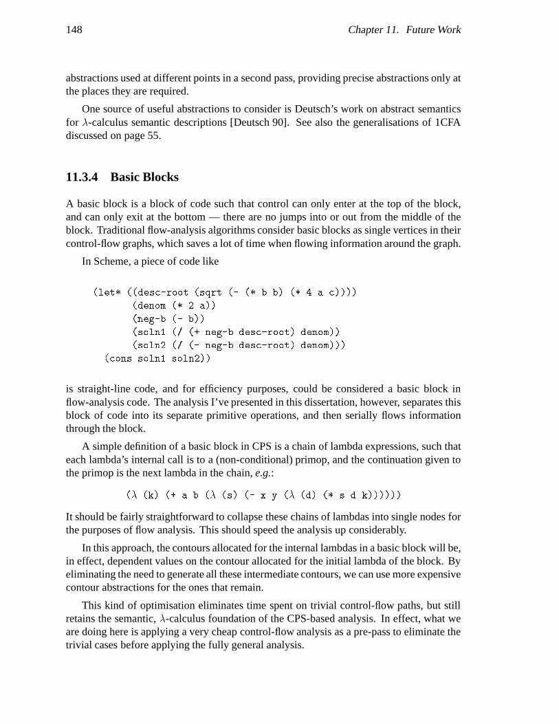
148 Chapter 11. Future Work
abstractions used at different points in a second pass, providing precise abstractions only atthe places they are required.
One source of useful abstractions to consider is Deutsch’s work on abstract semanticsfor �-calculus semantic descriptions [Deutsch 90]. See also the generalisations of 1CFAdiscussed on page 55.
11.3.4 Basic Blocks
A basic block is a block of code such that control can only enter at the top of the block,and can only exit at the bottom — there are no jumps into or out from the middle of theblock. Traditional flow-analysis algorithms consider basic blocks as single vertices in theircontrol-flow graphs, which saves a lot of time when flowing information around the graph.
In Scheme, a piece of code like
(let* ((desc-root (sqrt (- (* b b) (* 4 a c))))
(denom (* 2 a))
(neg-b (- b))
(soln1 (/ (+ neg-b desc-root) denom))
(soln2 (/ (- neg-b desc-root) denom)))
(cons soln1 soln2))
is straight-line code, and for efficiency purposes, could be considered a basic block inflow-analysis code. The analysis I’ve presented in this dissertation, however, separates thisblock of code into its separate primitive operations, and then serially flows informationthrough the block.
A simple definition of a basic block in CPS is a chain of lambda expressions, such thateach lambda’s internal call is to a (non-conditional) primop, and the continuation given tothe primop is the next lambda in the chain, e.g.:
(� (k) (+ a b (� (s) (- x y (� (d) (* s d k))))))
It should be fairly straightforward to collapse these chains of lambdas into single nodes forthe purposes of flow analysis. This should speed the analysis up considerably.
In this approach, the contours allocated for the internal lambdas in a basic block will be,in effect, dependent values on the contour allocated for the initial lambda of the block. Byeliminating the need to generate all these intermediate contours, we can use more expensivecontour abstractions for the ones that remain.
This kind of optimisation eliminates time spent on trivial control-flow paths, but stillretains the semantic, �-calculus foundation of the CPS-based analysis. In effect, what weare doing here is applying a very cheap control-flow analysis as a pre-pass to eliminate thetrivial cases before applying the fully general analysis.
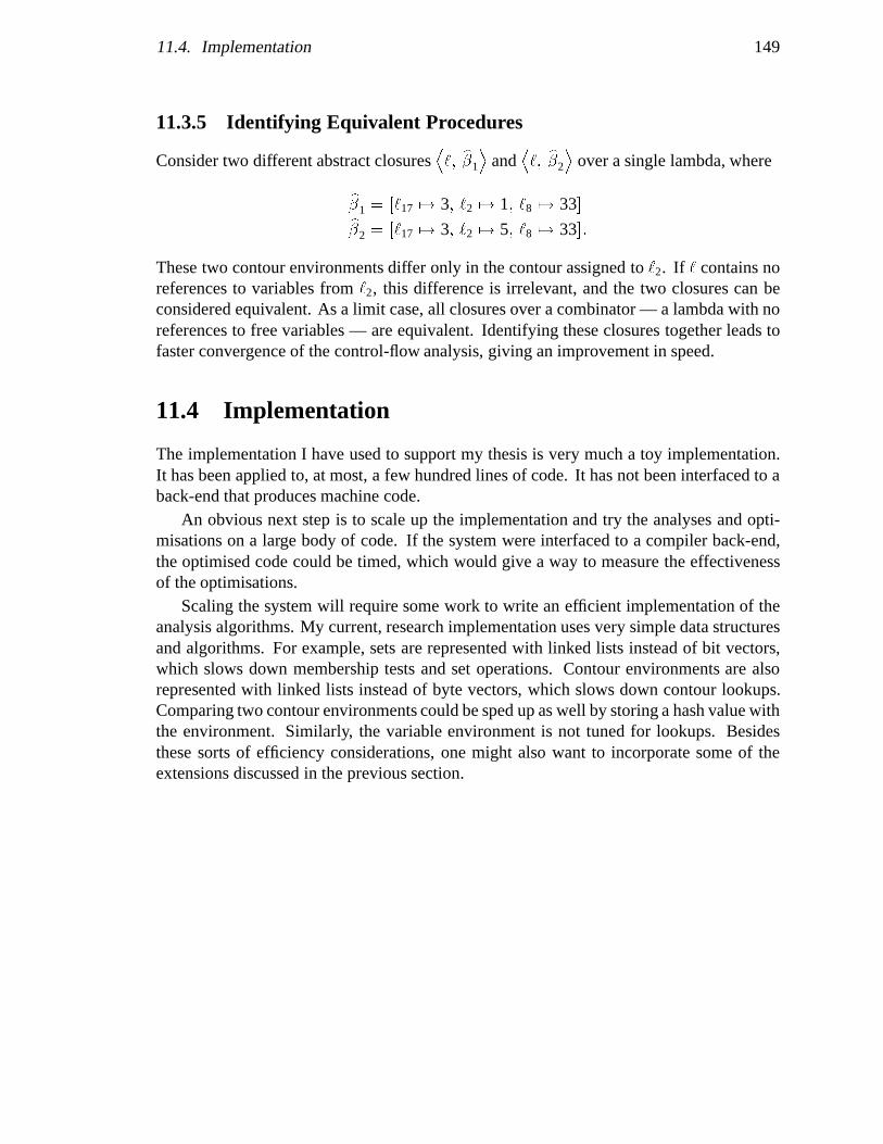
11.4. Implementation 149
11.3.5 Identifying Equivalent Procedures
Consider two different abstract closuresD`; b�1
Eand
D`; b�2
Eover a single lambda, where
b�1 =�`17 7! 3; `2 7! 1; `8 7! 33
�b�2 =
�`17 7! 3; `2 7! 5; `8 7! 33
�:
These two contour environments differ only in the contour assigned to `2. If ` contains noreferences to variables from `2, this difference is irrelevant, and the two closures can beconsidered equivalent. As a limit case, all closures over a combinator — a lambda with noreferences to free variables — are equivalent. Identifying these closures together leads tofaster convergence of the control-flow analysis, giving an improvement in speed.
11.4 Implementation
The implementation I have used to support my thesis is very much a toy implementation.It has been applied to, at most, a few hundred lines of code. It has not been interfaced to aback-end that produces machine code.
An obvious next step is to scale up the implementation and try the analyses and opti-misations on a large body of code. If the system were interfaced to a compiler back-end,the optimised code could be timed, which would give a way to measure the effectivenessof the optimisations.
Scaling the system will require some work to write an efficient implementation of theanalysis algorithms. My current, research implementation uses very simple data structuresand algorithms. For example, sets are represented with linked lists instead of bit vectors,which slows down membership tests and set operations. Contour environments are alsorepresented with linked lists instead of byte vectors, which slows down contour lookups.Comparing two contour environments could be sped up as well by storing a hash value withthe environment. Similarly, the variable environment is not tuned for lookups. Besidesthese sorts of efficiency considerations, one might also want to incorporate some of theextensions discussed in the previous section.

150 Chapter 11. Future Work

Chapter 12
Related Work
The fields of abstract semantic interpretation, higher-order language optimisation, and data-flow analysis are far too large to cover comprehensively. In this chapter I will cover workby others that is either fundamental or directly relevant to my research. I will focus onNSAS-based analyses. Discussions of work that is relevant to the particular optimisationsI’ve presented in this dissertation are found in the associated chapters.
12.1 Early Abstract Interpretation: the Cousots andMycroft
The seminal work on non-standard abstract interpretation is by the Cousots [Cousot 77,Cousot 79]. Starting with a standard semantics that maps process states to process states,they introduce a “static semantics” (what Mycroft calls a “collecting semantics”) thatcollects all possible states the process evolves through during execution of the program.Any compile-time analysis is then an abstraction of this static semantics. These abstractionsare defined by an abstraction function (and its related inverse, called a “concretisationfunction”). The Cousots define necessary conditions for abstraction functions to obeytypical compile-time properties (e.g., safely approximating the static semantics). The setof suitable abstractions is shown to have a lattice structure.
The Cousots’ work, however, is all in terms of imperative, non-functional languages,developed using a flowchart-based intermediate representation. Mycroft’s dissertation[Mycroft 81] extends the idea of abstract semantics to a functional language. His mainintended application is strictness analysis for normal-order languages — spotting opportu-nities to evaluate function arguments with call-by-value rules instead of call-by-need ruleswithout changing the result of the program. Mycroft’s semantics uses a complex semanticstructure called a powerdomain. His analyses are also developed for first-order, normal-order functional languages. My thesis is concerned with higher-order, applicative-orderlanguages that allow side-effects.
A useful collection of work on abstract semantic interpretation is Abstract Interpretationof Declarative Languages [Abramsky 87].
151

152 Chapter 12. Related Work
12.2 Hudak
Closer to my thesis, and in fact a direct influence on my work, is the work of Hudakand his students. Hudak’s paper, “Collecting Interpretations of Expressions” [Hudak 86],defines the problem of a collecting semantics for several variants of functional language —including the higher-order case. Hudak states the critical question of abstract analysis in afunctional setting: “what are all possible values to which the expression exp might evaluateduring program execution?” To answer this question, Hudak introduces the idea of a cachefunction that collects this information. This is related to the cache function that mycontrol-flow semantics computes, with two distinctions. First, my semantics only collectsprocedural values, ignoring other data. This distinction is merely one of focus; it is trivialto modify my semantics to collect abstractions of other datatypes, as well (as in the caseof performing constant propagation — see section 7.3). Secondly, my cache functions arefiner-grained than Hudak’s because they don’t lump all evaluations of a single expressiontogether. That is, where Hudak’s caches have functionality Exp ! Val, my caches havefunctionality Exp� Env ! Val.
Hudak abandons Mycroft’s powerdomains for a simpler powerset construction, which Ihave also used in my semantics. Hudak’s constructions are distinguished from the Cousots’in that his semantics are not presented as the closure of a state!state function. Instead,his semantics functions directly compute the cache produced by evaluating an expression.Interestingly, in the CPS representation I use, these two approaches converge. Althoughthe structure and intent is similar to Hudak’s, the CPS representation forces a kind of linearstate-to-state transition as evaluation proceeds. This is reflected in the names of the FStateand CState sets, implying that they represent the process states that the interpreter evolvesthrough during program execution. I find this dual view to be one of the attractions of theCPS representation: it provides the functional elegance and power of a representation basedon the �-calculus, while simultaneously allowing for a low-level, serialised, operationalinterpretation.
While Hudak does not provide for computable abstractions for the higher-order case,“Collecting Interpretation of Expressions” provides the general framework for the researchthat I’ve done to support my thesis.
Other Hudak papers apply his framework to particular analyses. For example, Hudakand Young have developed a strictness analysis for higher-order languages [Hudak+ 86b].Hudak has also designed an analysis for determining when functional array updates canbe done destructively [Hudak 86b]. However, the higher-order strictness analysis is notguaranteed to terminate, and the update analysis is restricted to first-order languages.
In general, Hudak’s work has focussed on purely functional, side-effectless, normal-order languages. The languages I am interested in — Scheme and ML — are applicativeand allow side-effects. Further, the set of optimisations I have considered for applicationsare the classical data-flow analysis optimisations. These optimisations have largely beenignored by the functional-language community. (This is not to say that these optimisationscould not be adapted to functional, normal-order languages. But compiler technology forthese sorts of languages has not yet progressed to the stage where this is a pressing need.)

12.3. Higher-Order Analyses: Deutsch and Harrison 153
12.3 Higher-Order Analyses: Deutsch and Harrison
As I have mentioned above, most work on abstract semantic interpretation has not dealt withthe full set of features that languages like Scheme or ML provide. Higher-order languagesare rarely treated, and when they are, side-effects are ignored. Two other recent researchefforts carried out independently and simultaneously with my own, however, address all ofthese issues, and so deserve special mention.
Deutsch has developed an analysis for determining the lifetimes of dynamically allocateddata at compile time [Deutsch 90]. This allows explicit deallocation of data structures thatwould otherwise have to be garbage collected, and the functional updating of aggregate datastructures by destructively modifying them. Deutsch’s intended application is optimisingsemantic specifications of programming languages. Since he deals with a higher-orderlanguage that allows side-effects, however, his techniques apply to Scheme and ML aswell.
Deutsch’s analysis is defined in terms of an intermediate representation that is somewhatlike assembler for a stack machine or Landin’s SECD machine [Landin 64]. I believethis representation is not well suited for program transformation and optimisation. Anintermediate representation based on a stack machine isn’t a high-level representation thatpermits interesting source-to-source transformations; neither is it a low-level representationthat exposes interesting properties of the program in terms of the actual target architecture.In contrast, CPS has the ability to span both ends of this representation spectrum simplyby choosing an appropriate set of primops. Steele made this claim for CPS as a generalframework for expressing different levels of representation [Steele 78]; Kelsey exploits thisproperty in his transformational compiler [Kelsey 89]. Further, since Deutsch’s semantics isa direct, stack-oriented semantics, it requires separate domains and equations for proceduresand continuations, whereas a CPS-based representation is much simplified by unifying allcontrol structures as procedures.
One of the most interesting technical aspects of Deutsch’s work is the “structuredabstraction” approach he takes to developing his abstract semantics. The idea is to defineabstractions for composite domains in terms of the domain’s structure and abstractions forits component subdomains. For example, if we have a cross-product domain A� B, thenwe can develop a “generic” abstraction function �� for cross-products, expressed in termsof abstraction functions �A and �B for the A and B components of the domain.
The advantage of this approach is twofold. First, we can develop a “toolbox” of ab-stractions for the basic mathematical constructs, such as sets, vectors, series, and functions.After proving that these abstractions satisfy some basic properties in isolation, we caneasily verify the correctness of abstractions built with these building blocks. Factoring thecorrectness proofs in this way simplifies the math in an elegant way.
Further, if we have several abstractions for, say, cross-products, then we can swapbetween these abstractions in a given application. While the different cross-product ab-stractions will have different cost/precision properties, they will be interchangeable withrespect to correctness considerations. This sort of modularity allows for easy experimenta-tion with different abstractions for a given analysis.

154 Chapter 12. Related Work
Structure abstractions are first mentioned in a paper by the Cousots’ [Cousot 79].Deutsch’s work, however, gives a strong example of this technique in application.1
Harrison has also developed semantically-based analyses for Scheme, with the intentionof parallelising Scheme programs [Harrison 89]. For example, he performs analysis todisambiguate structure aliasing in order to eliminate spurious edges in the graph of read/writedependencies that limits available parallelism.
Harrison handles full Scheme. His intermediate abstraction, again, is an imperative,non-CPS intermediate representation. Harrison’s work takes a coarse-grained view ofprocedures. His semantics is tuned to handle procedures that have roughly the samesize and functionality of FORTRAN or C procedures. His intermediate representation doesnot use lambdas for “intraprocedural” control structures: goto’s, conditional branches,loops and so forth. Instead, there are special, assembler-like syntactic constructs for eachof these structures. This increases the complexity of his semantics. Like Deutsch, hisnon-CPS semantics requires a separate (and complex) domain for continuations, and hissemantics equations must have separate cases to handle call/cc, procedure call, return, andcontinuation invocation, which greatly increases the size and complexity of his semantics.
Harrison’s semantics is also non-tail-recursive, which fits together with his focus onprocedures-as-subroutines. His semantics has the general structure of the Cousot-stylestate-to-state functions, as opposed to the Hudak-style direct semantics.
An interesting technical aspect of Harrison’s work is his contour abstraction, whichis based on finite regular expressions over relative procedure call/return sequences. Thisis an abstraction that is well matched to his focus on subroutine boundaries. Note thatthis abstraction could be adapted to my framework. Suitably modified to account for tail-recursive procedure calls, Harrison’s abstraction might work well for the coarse-grainedprocedural boundaries for which it was designed. (Whereas other abstractions could beused for the finer-grained lambdas, giving a sort of hybrid abstraction. See section 11.3.3.)
In contrast to Harrison’s, my work takes a fine-grained view of procedures. My in-termediate representation represents all transfers of control with a tail-recursive procedurecall. This provides a uniform representation for control flow that simplifies the analysismachinery. While Harrison focusses on inter-procedural control and data flow, I am moreinterested in intra-procedural applications — the classical data-flow optimisations, in afunctional, higher-order setting.
Harrison’s work does not delve into as much detail on his analysis as I have in thisdissertation. Harrison skips many of the more tedious correctness proofs that I’ve presentedin chapter 4. He also doesn’t present details of his algorithms or prove their correctness.This is almost certainly due to time and space restrictions: Harrison’s semantic analysis isonly one part of his research on interprocedural analysis and parallelisation.
Finally, neither Harrison, Deutsch, nor any of the other researchers I’ve discussed inthis chapter have dealt with the environment problem. The solution I present in chapter 8is a unique contribution, to the best of my knowledge.
1Deutsch’s research report describes more of the structured abstractions than the conference publication.
Chapter 13
Conclusions
My research makes the following contributions:
� A solution to the control-flow problem for higher-order languages, where the allowedlanguage features includes side-effects and call/cc.
� A theoretical foundation for this analysis, complete with correctness proofs.
� Algorithms to compute the analysis, again, complete with correctness proofs.
� Example applications using the analysis.
� Reflow analysis: a powerful extension for solving the environment problem.
� Example applications using this extension.
This all adds up to a general framework for performing data-flow analysis for higher-orderlanguages.
As I stated at the beginning of this dissertation, my thesis is that control-flow analysisis feasible and useful for higher-order languages. The analysis, algorithms, and associ-ated correctness proofs should establish its feasibility. The example optimisations shouldestablish its utility.
A secondary thesis of this work might be called the “CPS representation thesis.” Ihope I have strengthened the case for CPS-based compiler intermediate representations –their simplicity, theoretical underpinnings, and power support the transition of compilers forhigher-order languages into the highly-optimising niche. With CPS, we arrive at a new viewof traditional data-flow optimisations in a functional, higher-order setting: one that empha-sises variable binding over variable assignment, and where the basic control/environmentconstruct is lambda/procedure-call.
A closing thought: As we’ve seen, control-flow analysis in higher-order languages isreally data-flow analysis in the higher-order procedure case. As procedural data flows topoints in the control-flow graph, new paths become possible, opening up new routes fordata flow, and so the loop is closed. Thus the title of this dissertation is perhaps a bit
155

156 Chapter 13. Conclusions
misleading. In order to solve the control-flow problem, we must also solve the data-flowproblem, and our analysis must further involve considerations of environment structure.
This is a fundamental property of having the lambda operator in our language. Lambdais an operator that simultaneously establishes data, control, and environment structure:
� Evaluating a lambda creates a closure, which is a first-class data structure.
� A lambda is a control point to which control can be transferred by procedure call; ina CPS representation, lambda is the fundamental control structure.
� Entering a lambda causes environment structure to be established by the bindingof the lambda’s parameters; again, in higher-order languages lambda binding is thefundamental environment structure.
In the lambda operator, all three fundamental program structures — data, control, andenvironment — meet and intertwine. Thus, any analysis technique for a higher-orderlanguage must be prepared to handle the three facets of lambda. In essence, the work inthis dissertation has been the application of classical data-flow analysis in the presence oflambda.
Appendix A
1CFA Code Listing
Dear Mr. Shivers,Your code horrified me . . . patches to failures. . . not principled
— mob 9/22/90
. . . the techniques described in your . . . lispposting are quite frankly horrid . . . isn’t evenlegal . . . it breaks enormously . . . ??? bogus!!
— ted 9/22/90
This appendix contains a code listing for my 1CFA implementation. Before running thisanalysis, a modified copy of the ORBIT compiler’s front end is used to CPS-convert thecode and produce a syntax tree. This tree is the input to the 1CFA analysis listed here.
A.1 Preliminaries
A.1.1 Details of the dialect
The program is written in T, a dialect of Scheme with additional extensions from severalmacro packages. Here is a brief description of the various macro packages that are used inthis code.
The UCI LISP for macro is syntactic sugar for map-type loops. The expression
(for (x in <list1>)
(y in <list2>)
(save (f (- y x))))
expands into
(map (� (x y) (f (- y x))) <list1> <list2>)
157

158 Appendix A. 1CFA Code Listing
If the do keyword is used instead of the save keyword, then the macro expands into afor-each (in T, a walk) instead of a map.
A more powerful iteration construct is the Yale loop macro. Without giving a detaileddescription of the entire macro, the following example should give the general structure:
(loop (initial (m 0 (max m x)))
(for x in l)
(incr i .in 0 to (vector-length v))
(do (set (vref v i) x))
(result m))
This expression iterates over a list l and a vector v, storing the elements of l into v. Theloop terminates when it runs off the end of either l or v. The .in keyword means the rangeof the i variable includes 0 but not (vector-length v) (in. is the other way around;.in. includes both endpoints; in includes neither). The variable m is initialised to 0; eachtime through the loop, it is updated to be the largest element scanned. This maximum valueis returned as the result of the loop.
The def-structmacro is macro support for T’s record structures. The structure
(def-struct ship
x
y
(size 1000))
defines a ship record with three fields. The sizefield is initialised by default to 1000. Thisinstance of def-structdefines three accessor functions: ship:x, ship:yand ship:size.These slots can be assigned with the T set form:
(set (ship:x shipa) 100)
There is also a predicate ship? that returns true only when applied to ship structures.Finally, the constructor macro ship:new is used to create new structures, with record slotsoptionally specified by name. For example,
(ship:new x 7 size 4)
creates a new ship structure, with the x field initialised to 7, the size field initialised to 4,and the y field unspecified.
I use ? as an abbreviation for cond. The T cond form has a useful extension. If a clauseis of the form
(test => fn)then if test is true, fn is applied to the value it produces. T also defines the else constantto be a true value. So the expression
(? ((assq var alist) => cdr)
(else (error "unbound variable ~s" var)))

A.1. Preliminaries 159
looks up a variable binding in an alist, signalling an error if the variable is unbound.
Finally, this code uses a small package for manipulating lists as sets. The functionset:new is identical to the list function, so (set:new 2 3 5) constructs a set (list) ofthe first three primes. The procedure
(union elt= seta setb)
returns the union of seta and setb, where the elements of the list are compared with theelt= function. The macro
(difference-and-union elt= s1 s2 (d u) . body)
computes the difference and union of sets s1 and s2. The body forms are then executed inan environment with d bound to the difference and u bound to the union.
A.1.2 The syntax tree
The syntax tree produced by the ORBIT front end is built with the nodes shown in figureA.1. I’ll only describe here the parts of the node data structures that are useful to the 1CFAanalysis. The node data structures are not defined by the def-structmacro, and the fieldsyntax is different. The procedure that accesses the field component of node type node isnamed node-field, not node:field. For example, reference node r’s variable field isaccessed with (reference-variable r).
Reference A variable reference node has a single field, the variable node it references.
Primop Every occurence of a primop in the code tree is a distinct primop node. A primopnode has one field, its value. This is a separate primop def-struct, defined as:
(def-struct primop
id ; Name of this primop
ic ; Single ic or a vector of ic's
1cfa-propagator) ; Defines action of F
(In fact, there are a few other fields in the primop def-struct, but they are not used bythe 1CFA analysis.) The primop:ic field holds either a single call node (for simpleprimops), or a two-element vector of call nodes (for conditional primops). These callnodes are the ic markers for the primop. Note that all occurrences of a primop share asingle primop def-struct, so they all share the same ic nodes. This is acceptable in the1CFA abstraction, since the continuation calls from the different occurrences of theprimop will be distinguished in the call cache by the the contour environment part ofthe
Dic; b�E call context. The primop:1cfa-propagatorfield holds a procedure that
defines bF for this primop — see the functionalise procedure in the code listing.
Literal A literal node has no fields that are useful for control-flow analysis.
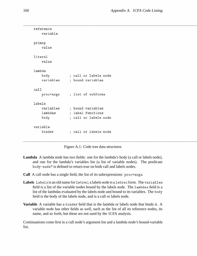
160 Appendix A. 1CFA Code Listing
reference
variable
primop
value
literal
value
lambda
body ; call or labels node
variables ; bound variables
call
proc+args ; list of subforms
labels
variables ; bound variables
lambdas ; label functions
body ; call or labels node
variable
binder ; call or labels node
Figure A.1: Code tree data structures
Lambda A lambda node has two fields: one for the lambda’s body (a call or labels node),and one for the lambda’s variables list (a list of variable nodes). The predicatebody-node? is defined to return true on both call and labels nodes.
Call A call node has a single field, the list of its subexpressions: proc+args.
Labels Labels is an old name for letrec; a labels node is a letrec form. The variablesfield is a list of the variable nodes bound by the labels node. The lambdas field is alist of the lambdas evaluated by the labels node and bound to its variables. The bodyfield is the body of the labels node, and is a call or labels node.
Variable A variable has a binder field that is the lambda or labels node that binds it. Avariable node has other fields as well, such as the list of all its reference nodes, itsname, and so forth, but these are not used by the 1CFA analysis.
Continuations come first in a call node’s argument list and a lambda node’s bound-variablelist.
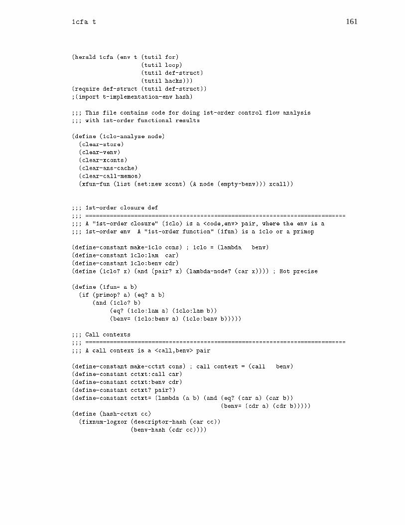
1cfa.t 161
(herald 1cfa (env t (tutil for)
(tutil loop)
(tutil def-struct)
(tutil hacks)))
(require def-struct (tutil def-struct))
;(import t-implementation-env hash)
;;; This file contains code for doing 1st-order control flow analysis
;;; with 1st-order functional results.
(define (1clo-analyse node)
(clear-store)
(clear-venv)
(clear-xconts)
(clear-ans-cache)
(clear-call-memos)
(xfun-fun (list (set:new xcont) (A node (empty-benv))) xcall))
;;; 1st-order closure def
;;; ===========================================================================
;;; A "1st-order closure" (1clo) is a <code,env> pair, where the env is a
;;; 1st-order env. A "1st-order function" (1fun) is a 1clo or a primop.
(define-constant make-1clo cons) ; 1clo = (lambda . benv)
(define-constant 1clo:lam car)
(define-constant 1clo:benv cdr)
(define (1clo? x) (and (pair? x) (lambda-node? (car x)))) ; Not precise
(define (1fun= a b)
(if (primop? a) (eq? a b)
(and (1clo? b)
(eq? (1clo:lam a) (1clo:lam b))
(benv= (1clo:benv a) (1clo:benv b)))))
;;; Call contexts
;;; ===========================================================================
;;; A call context is a <call,benv> pair.
(define-constant make-cctxt cons) ; call context = (call . benv)
(define-constant cctxt:call car)
(define-constant cctxt:benv cdr)
(define-constant cctxt? pair?)
(define-constant cctxt= (lambda (a b) (and (eq? (car a) (car b))
(benv= (cdr a) (cdr b)))))
(define (hash-cctxt cc)
(fixnum-logxor (descriptor-hash (car cc))
(benv-hash (cdr cc))))

162 Appendix A. 1CFA Code Listing
;;; Answer cache code
;;; ===========================================================================
;;; Ans cache maps a call context (a <call,benv> pair) to a set of 1funs
;;; that could have been called from CALL in context BENV.
(lset *ans-cache* nil)
(define (clear-ans-cache)
(set *ans-cache* (make-hash-table cctxt? hash-cctxt cctxt= t 'ans-cache)))
;;; Record in the ans cache that we called FUNS from call context <CALL,BENV>
(define (record-call call benv funs)
(modify (table-entry *ans-cache* (make-cctxt call benv))
(lambda (entry) (union 1fun= entry funs))))
;;; Global variable environment code
;;; ===========================================================================
;;; The VEnv maps a contour (a lambda or labels node) and a var to a
;;; set of 1clo's. (but not primops)
(lset *venv* nil)
(lset *venv-stamp* 0) ; When we alter the venv, bump this guy.
(define (clear-venv)
(set *venv* (make-hash-table pair?
(lambda (x)
(fixnum-logxor (descriptor-hash (car x))
(descriptor-hash (cdr x))))
(lambda (k1 k2)
(and (eq? (car k1) (car k2))
(eq? (cdr k1) (cdr k2))))
t
'venv-table))
(set *venv-stamp* 0))
(define (venv-lookup contour var)
(table-entry *venv* (cons contour var)))
(define (venv-augment contour vars arglis)
(for (v in vars)
(argset in arglis)
(do (let* ((index (cons contour v))
(entry (table-entry *venv* index)))
(difference-and-union 1fun= argset entry (d u)
(? (d
(set (table-entry *venv* index) u)
(set *venv-stamp* (fx+ *venv-stamp* 1)))))))))

1cfa.t 163
;;; Contour env code
;;; ===========================================================================
(define-integrable (empty-benv) '())
(define (benv-lookup benv binder)
(? ((assq binder benv) => cdr)
(else (error "benv-lookup: couldn't find ~a in ~a" binder benv))))
(define-integrable (benv-augment benv binder contour); benv[binder |-> contour]
(cons (cons binder contour) benv))
(define (benv= a b) ; Assumes the benv's are over the same code, as it were.
(assert (every? (lambda (a b) (eq? (car a) (car b))) a b)) ; paranoia
(every? (lambda (a-entry b-entry) (eq? (cdr a-entry) (cdr b-entry)))
a b))
(define-constant (benv-hash benv)
(loop (for elt in benv)
(initial (val 42 (fixnum-logxor (descriptor-hash (cdr elt)) val)))
(result val)))
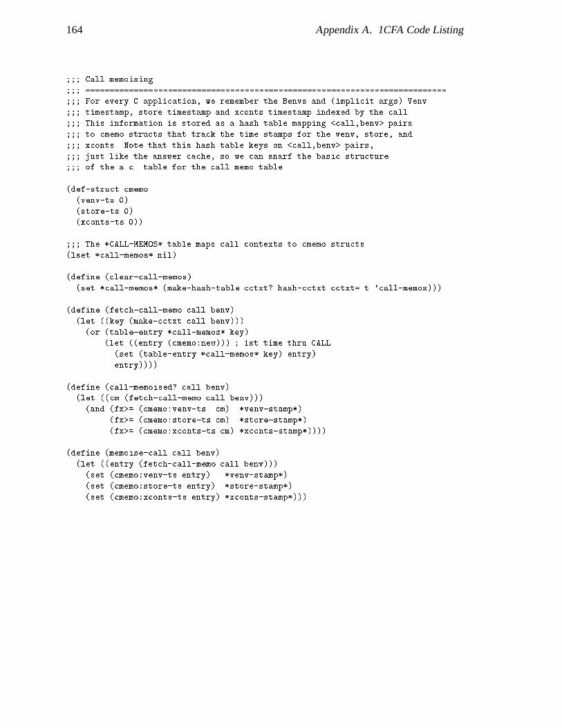
164 Appendix A. 1CFA Code Listing
;;; Call memoising
;;; ===========================================================================
;;; For every C application, we remember the Benvs and (implicit args) Venv
;;; timestamp, store timestamp and xconts timestamp indexed by the call.
;;; This information is stored as a hash table mapping <call,benv> pairs
;;; to cmemo structs that track the time stamps for the venv, store, and
;;; xconts. Note that this hash table keys on <call,benv> pairs,
;;; just like the answer cache, so we can snarf the basic structure
;;; of the a.c. table for the call memo table.
(def-struct cmemo
(venv-ts 0)
(store-ts 0)
(xconts-ts 0))
;;; The *CALL-MEMOS* table maps call contexts to cmemo structs.
(lset *call-memos* nil)
(define (clear-call-memos)
(set *call-memos* (make-hash-table cctxt? hash-cctxt cctxt= t 'call-memos)))
(define (fetch-call-memo call benv)
(let ((key (make-cctxt call benv)))
(or (table-entry *call-memos* key)
(let ((entry (cmemo:new))) ; 1st time thru CALL
(set (table-entry *call-memos* key) entry)
entry))))
(define (call-memoised? call benv)
(let ((cm (fetch-call-memo call benv)))
(and (fx>= (cmemo:venv-ts cm) *venv-stamp*)
(fx>= (cmemo:store-ts cm) *store-stamp*)
(fx>= (cmemo:xconts-ts cm) *xconts-stamp*))))
(define (memoise-call call benv)
(let ((entry (fetch-call-memo call benv)))
(set (cmemo:venv-ts entry) *venv-stamp*)
(set (cmemo:store-ts entry) *store-stamp*)
(set (cmemo:xconts-ts entry) *xconts-stamp*)))

1cfa.t 165
;;; A & C
;;; ===========================================================================
(define (A form benv)
(? ((reference-node? form)
(let ((var (reference-variable form)))
(venv-lookup (benv-lookup benv (variable-binder var)) var)))
((primop-node? form) (set:new (primop-value form)))
((literal-node? form) (empty-set))
((lambda-node? form) (set:new (make-1clo form benv)))
(else (error "type error"))))
(define (C form benv)
(assert (body-node? form))
(? ((not (call-memoised? form benv))
(memoise-call form benv)
(if (call-node? form) (C-call form benv)
(C-labels form benv)))))
(define (C-call call benv)
(assert (call-node? call))
(destructure (( (fun . args) (call-proc+args call) ))
(let ((funset (A fun benv))
(arglis (for (arg in args) (save (A arg benv)))))
(record-call call benv funset)
(for (f in funset)
(do ((functionalise f) arglis call))))))
(define (functionalise funspec)
(? ((primop? funspec) (P funspec))
((eq? funspec xfun) xfun-fun) ; Calling the external function
((eq? funspec xcont) xcont-fun) ; Calling the external continuation.
(else
(let* ((lam (1clo:lam funspec))
(body (lambda-body lam))
(formals (lambda-variables lam))
(nformals (length formals))
(benv (1clo:benv funspec)))
(lambda (arglis b)
(? ((fx= nformals (length arglis))
(venv-augment b formals arglis)
(C body (benv-augment benv lam b)))))))))
(define (C-labels lab benv)
(let ((benv (benv-augment benv lab lab)))
(venv-augment lab
(labels-variables lab)
(for (f in (labels-lambdas lab))
(save (A f benv))))
(C (labels-body lab) benv)))

166 Appendix A. 1CFA Code Listing
;;; Primop definitions
;;; ===========================================================================
;;; Since primops aren't 1st-class, we can statically check their
;;; argspectrum, so no need to check at runtime.
(define-integrable (P prim) (primop:1cfa-propagator prim))
(define-syntax (define-p prim fun)
(let ((name (concatenate-symbol 'p/ prim))
(syn-name (concatenate-symbol 'primop/ prim)))
`(block (define ,name ,fun)
(set (primop:1cfa-propagator ,syn-name) ,name))))
(define-syntax (define-simple-p prim)
(let ((syn-name (concatenate-symbol 'primop/ prim)))
`(define-p ,prim
(lambda (arglis contour)
(destructure (( (c a b) arglis ))
(let ((ic (primop:ic ,syn-name))
(benv (primop-env ,syn-name contour)))
;; record a call to the conts from ctxt <ic, [prim -> contour]>
(record-call ic benv c)
(for (f in c)
(do ((functionalise f) <@> ic)))))))))
(define-simple-p +)
(define-simple-p *)
(define-simple-p -)
(define-p test
(lambda (arglis contour)
(destructure (( (c a p . v) arglis ))
(let* ((benv (primop-env primop/test contour))
(ic-vec (primop:ic primop/test))
(ic0 (vref ic-vec 0))
(ic1 (vref ic-vec 1)))
;; record a call to C conts from context <ic0test, [test -> contour]>
(record-call ic0 benv c)
(for (f in c)
(do ((functionalise f) <> ic0)))
;; record a call to A conts from context <ic1test [test -> contour]>
(record-call ic1 benv a)
(for (f in a)
(do ((functionalise f) <> ic1)))))))
(define (primop-env primop contour)
(benv-augment (empty-benv) primop contour))
(define-constant <@> (list (empty-set))) ; arglis of 1 empty set.
(define-constant <> '()) ; arglis of 0 length
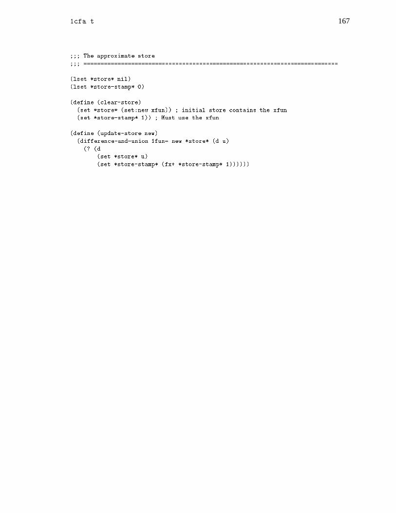
1cfa.t 167
;;; The approximate store
;;; ===========================================================================
(lset *store* nil)
(lset *store-stamp* 0)
(define (clear-store)
(set *store* (set:new xfun)) ; initial store contains the xfun.
(set *store-stamp* 1)) ; Must use the xfun...
(define (update-store new)
(difference-and-union 1fun= new *store* (d u)
(? (d
(set *store* u)
(set *store-stamp* (fx+ *store-stamp* 1))))))

168 Appendix A. 1CFA Code Listing
;;; (DEFINE-STORE-P prim args stashers ic-call-argv)
;;; ===========================================================================
;;; This is for defining primops that access or modify the store. This
;;; form defines a primop PRIM with arguments ARGS. The first element of
;;; ARGS is the continuation. STASHERS is a subset of the args. When this
;;; primop is invoked
;;; - A call from the primop's i.c. site to the continuations is recorded.
;;; - The stasher arguments are placed in the store.
;;; - The primop's continuations are called with the argument
;;; vector IC-CALL-ARGV, which is typically <@> or (LIST *STORE*).
;;;
;;; For example,
;;; (DEFINE-STORE-P NEW (C V) (V) <@>)
;;; define the NEW primop, which takes two arguments: a continuation C
;;; and a value V. The values passed in for V should be put in the store.
;;; NEW produces no procedures, so the continuation should be applied
;;; to the empty set @ -- that is, the arg vector <@>.
(define-syntax (define-store-p prim args stashers ic-call-argv)
(let ((syn-name (concatenate-symbol 'primop/ prim)))
`(define-p ,prim
(lambda (arglis contour)
(destructure (( ,args arglis ))
(let ((ic (primop:ic ,syn-name))
(benv (primop-env ,syn-name contour)))
;; record a call to the conts from ctxt <ic, [prim -> contour]>
(record-call ic benv c)
;; All stashed args -> store:
,@(for (s in stashers) (save `(update-store ,s)))
;; Do the ic call:
(for (f in ,(car args)) ; continuations
(do ((functionalise f) ,ic-call-argv ic)))))))))
(define-store-p new (c v) (v) <@>)
(define-store-p contents (c a) () (list *store*))
(define-store-p set (c a v) (v) <@>)
;;; The simple-minded CPS-converter assumes all expressions evaluate
;;; to exactly one value (so their continuations have one formal parameter).
;;; However, SET is not defined to produce a value. We hack this by assuming
;;; SET returns a constant (e.g., #f). So the abstract arg vec for the
;;; continuation call is <@>, not <>.
(define-store-p cons (c a d) (a d) <@>)
(define-store-p car (c a) () (list *store*))
(define-store-p cdr (c a) () (list *store*))
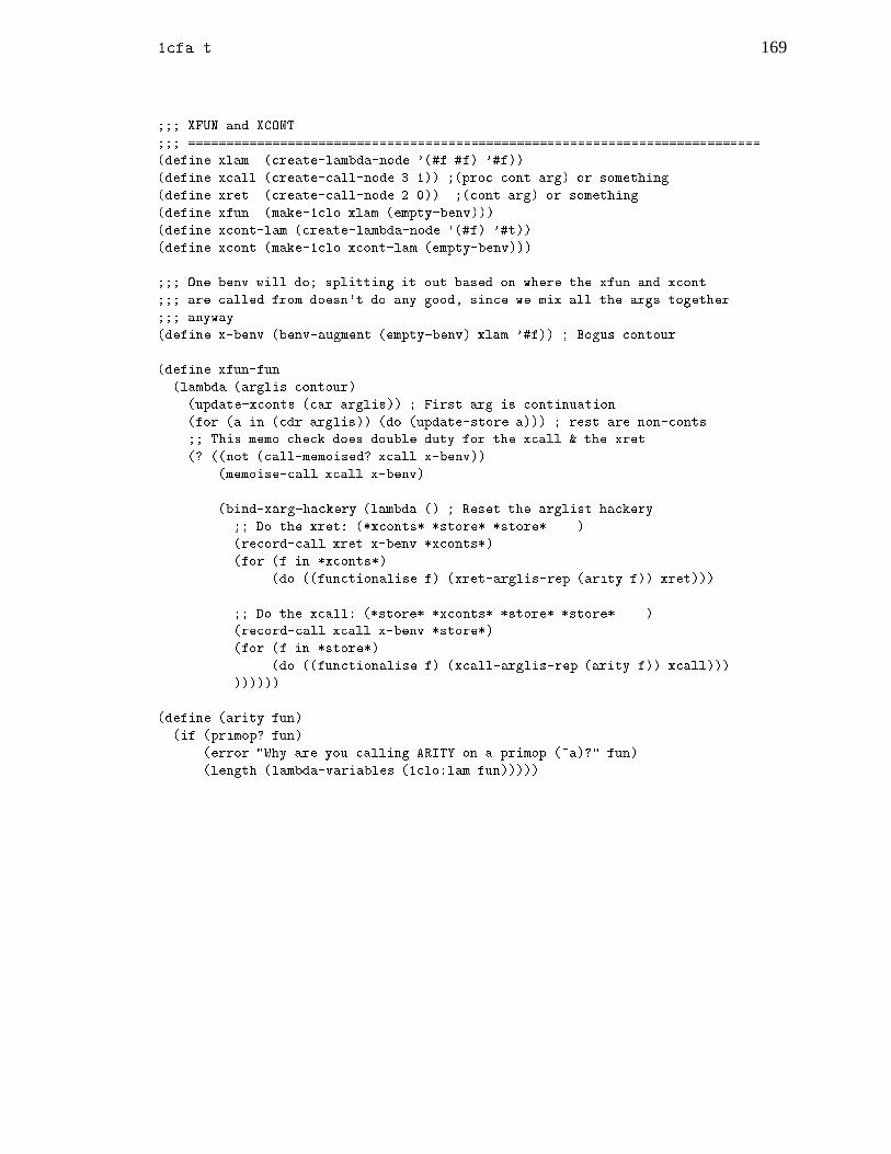
1cfa.t 169
;;; XFUN and XCONT
;;; ===========================================================================
(define xlam (create-lambda-node '(#f #f) '#f))
(define xcall (create-call-node 3 1)) ;(proc cont arg) or something.
(define xret (create-call-node 2 0)) ;(cont arg) or something.
(define xfun (make-1clo xlam (empty-benv)))
(define xcont-lam (create-lambda-node '(#f) '#t))
(define xcont (make-1clo xcont-lam (empty-benv)))
;;; One benv will do; splitting it out based on where the xfun and xcont
;;; are called from doesn't do any good, since we mix all the args together
;;; anyway.
(define x-benv (benv-augment (empty-benv) xlam '#f)) ; Bogus contour
(define xfun-fun
(lambda (arglis contour)
(update-xconts (car arglis)) ; First arg is continuation.
(for (a in (cdr arglis)) (do (update-store a))) ; rest are non-conts
;; This memo check does double duty for the xcall & the xret.
(? ((not (call-memoised? xcall x-benv))
(memoise-call xcall x-benv)
(bind-xarg-hackery (lambda () ; Reset the arglist hackery
;; Do the xret: (*xconts* *store* *store* ...)
(record-call xret x-benv *xconts*)
(for (f in *xconts*)
(do ((functionalise f) (xret-arglis-rep (arity f)) xret)))
;; Do the xcall: (*store* *xconts* *store* *store* ...)
(record-call xcall x-benv *store*)
(for (f in *store*)
(do ((functionalise f) (xcall-arglis-rep (arity f)) xcall)))
))))))
(define (arity fun)
(if (primop? fun)
(error "Why are you calling ARITY on a primop (~a)?" fun)
(length (lambda-variables (1clo:lam fun)))))
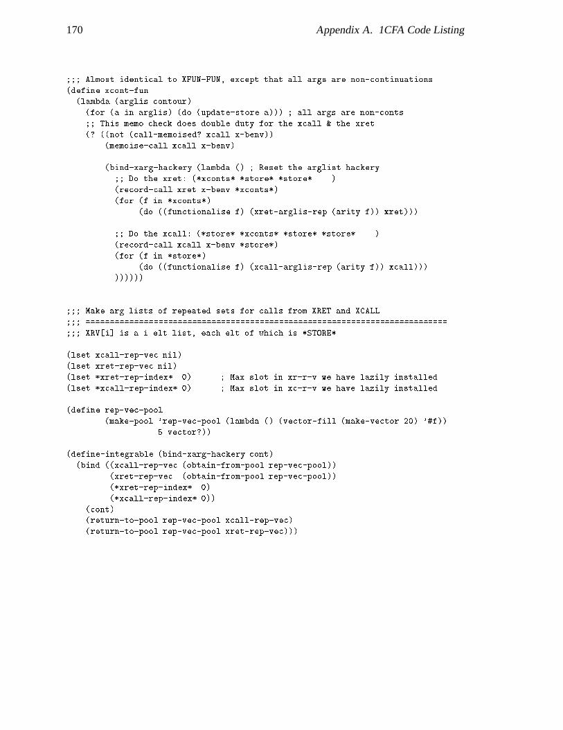
170 Appendix A. 1CFA Code Listing
;;; Almost identical to XFUN-FUN, except that all args are non-continuations.
(define xcont-fun
(lambda (arglis contour)
(for (a in arglis) (do (update-store a))) ; all args are non-conts
;; This memo check does double duty for the xcall & the xret.
(? ((not (call-memoised? xcall x-benv))
(memoise-call xcall x-benv)
(bind-xarg-hackery (lambda () ; Reset the arglist hackery
;; Do the xret: (*xconts* *store* *store* ...)
(record-call xret x-benv *xconts*)
(for (f in *xconts*)
(do ((functionalise f) (xret-arglis-rep (arity f)) xret)))
;; Do the xcall: (*store* *xconts* *store* *store* ...)
(record-call xcall x-benv *store*)
(for (f in *store*)
(do ((functionalise f) (xcall-arglis-rep (arity f)) xcall)))
))))))
;;; Make arg lists of repeated sets for calls from XRET and XCALL.
;;; ===========================================================================
;;; XRV[i] is a i elt list, each elt of which is *STORE*.
(lset xcall-rep-vec nil)
(lset xret-rep-vec nil)
(lset *xret-rep-index* 0) ; Max slot in xr-r-v we have lazily installed.
(lset *xcall-rep-index* 0) ; Max slot in xc-r-v we have lazily installed.
(define rep-vec-pool
(make-pool 'rep-vec-pool (lambda () (vector-fill (make-vector 20) '#f))
5 vector?))
(define-integrable (bind-xarg-hackery cont)
(bind ((xcall-rep-vec (obtain-from-pool rep-vec-pool))
(xret-rep-vec (obtain-from-pool rep-vec-pool))
(*xret-rep-index* 0)
(*xcall-rep-index* 0))
(cont)
(return-to-pool rep-vec-pool xcall-rep-vec)
(return-to-pool rep-vec-pool xret-rep-vec)))
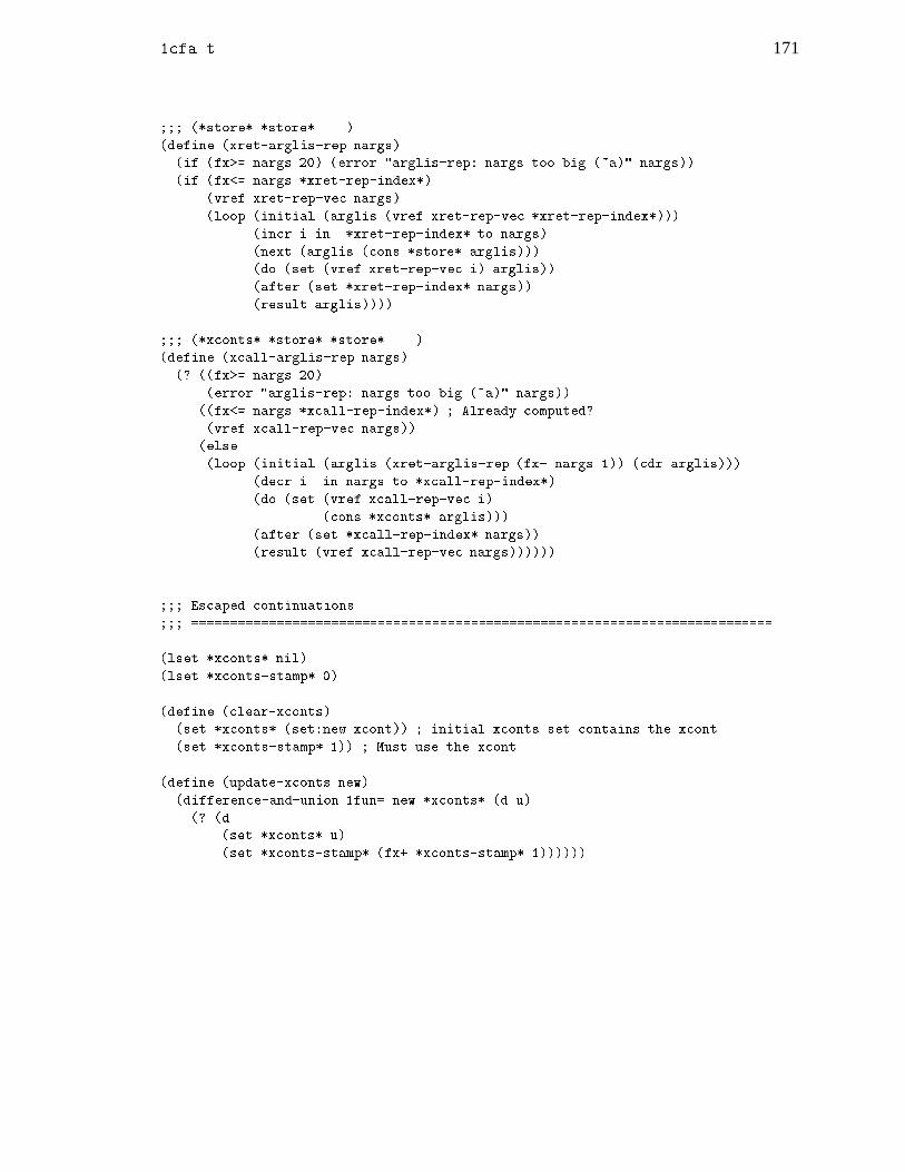
1cfa.t 171
;;; (*store* *store* ...)
(define (xret-arglis-rep nargs)
(if (fx>= nargs 20) (error "arglis-rep: nargs too big (~a)" nargs))
(if (fx<= nargs *xret-rep-index*)
(vref xret-rep-vec nargs)
(loop (initial (arglis (vref xret-rep-vec *xret-rep-index*)))
(incr i in. *xret-rep-index* to nargs)
(next (arglis (cons *store* arglis)))
(do (set (vref xret-rep-vec i) arglis))
(after (set *xret-rep-index* nargs))
(result arglis))))
;;; (*xconts* *store* *store* ...)
(define (xcall-arglis-rep nargs)
(? ((fx>= nargs 20)
(error "arglis-rep: nargs too big (~a)" nargs))
((fx<= nargs *xcall-rep-index*) ; Already computed?
(vref xcall-rep-vec nargs))
(else
(loop (initial (arglis (xret-arglis-rep (fx- nargs 1)) (cdr arglis)))
(decr i .in nargs to *xcall-rep-index*)
(do (set (vref xcall-rep-vec i)
(cons *xconts* arglis)))
(after (set *xcall-rep-index* nargs))
(result (vref xcall-rep-vec nargs))))))
;;; Escaped continuations
;;; ===========================================================================
(lset *xconts* nil)
(lset *xconts-stamp* 0)
(define (clear-xconts)
(set *xconts* (set:new xcont)) ; initial xconts set contains the xcont.
(set *xconts-stamp* 1)) ; Must use the xcont...
(define (update-xconts new)
(difference-and-union 1fun= new *xconts* (d u)
(? (d
(set *xconts* u)
(set *xconts-stamp* (fx+ *xconts-stamp* 1))))))

172 Appendix A. 1CFA Code Listing

Appendix B
Analysis Examples
B.1 Puzzle example
The first example is the little environment puzzle from page 120. The program is shownin figure B.1, both in Scheme and its CPS intermediate representation. In the CPS form,lambda and call expressions are subscripted with numeric labels (the particular labels usedare just those chosen by the T run-time system when printing out this example). As a specialcase, the CPS test primop requires its first argument to be a type or comparison predicate(e.g., integer? or eq?). This syntactic extension, inherited from the ORBIT front end, isequivalent to defining separate primops test-integer, test-eq?, and so forth.
CPS conversion introduces continuations into parameter lists and call expressions.ORBIT’s front-end and the analysis code listed in appendix A place these continuationarguments first in calls and parameter lists, e.g., (+ k 3 4). This has some programmingbenefits, but makes the code unreadable. So, I have edited the CPS code shown in thisappendix to use the continuation-last convention, e.g., (+ 3 4 k).
Applying the 1CFA program of appendix A to the puzzle example takes .67 seconds ofCPU time, running interpreted T on a DECstation 3100 PMAX. Applying the type-recoveryalgorithm of chapter 9 takes 5.1 seconds under the same configuration.
The information produced by the type-recovery algorithm is given in table B.2. Ifa variable is qualified with a call site, e.g. x(c51), then the type applies to the referenceoccuring in that call expression. Otherwise, the type applies to all references to that variable.So type recovery is able to correctly distinguish the two bindings of x, and determine fromthe type test (test fixnum? . . .) and the control-flow information that the x closed overin lambda l36 is a floating-point number.
The call cache produced by the 1CFA program is listed in figure B.3. It is simply adump of the *ans-cache* table constructed by the program. The output has been lightlyedited to improve its legibility. Each entry in the table maps a call context cc to a list ofabstract procedures called from that call context:
cc -> (proc1 proc2 . . .)
173

174 Appendix B. Analysis Examples
(� () (let ((f (� (x h)
(test (fixnum? x) (h) (� () x)))))
(f 3 (f 2.7 '#f))))
Scheme
(�34(k) (
41(�
42(f) (
43f 2.7 '#f (�
49(v) (
40f 3 v k))))
(�39(x h k1)
(44test fixnum? x
(�47() (
50h k1))
(�37() (
48k1 (�
36(k2) (
51k2 x))))))))
Annotated CPS
Figure B.1: Puzzle example
f, v, k, k1, k2 procx(c44) fixnum|floatx(c51) floath false|proc
Table B.2: Recovered type information
An abstract closure is a list whose head is a lambda and whose tail is an abstract contourenvironment. So
(l47 (l39 . c40) (l34 . xcall))
is the closure over lambda l47 with contour environment�l39 7! c40; l34 7! xcall
�.
This is the environment made in the 1CFA abstraction by entering lambda l34 from theexternal call, and subsequently entering lambda l39 from call c40. Most of the bindingcontours are given mnemonic names such as [top] or [if] that are listed in the initialcomment lines of the figure. The special symbols xcall, xret, xlam, xcont, ictest0, andictest1 represent the external call, external return, external lambda, external continuation,and internal call sites for the test primop, respectively.
Note that the
(xcall (xlam)) -> (l36 [else] [f2] [topcall])
edge in the call graph could be refined away by a post-type-recovery pass. In call context([f2] [topcall]), x is known to be bound to an integer, so the else branch is not taken.Removing this control-flow arc would also prune the extra arc
(c51 (l36 . xcall) [else] [f2] [topcall]) -> (xcont)

B.1. Puzzle example 175
;;; [top] (l34 . xcall)
;;; [let] (l42 . c41)
;;; [f1] (l39 . c43)
;;; [f1-ret] (l49 . c48)
;;; [f2] (l39 . c40)
;;; [if] (test . c44)
;;; [then] (l47 . ictest0)
;;; [else] (l37 . ictest1)
(xret (xlam)) -> (xcont)
(xcall (xlam)) -> ((l36 [else] [f2] [topcall])
(l34)
(xlam))
(c41 [topcall]) -> ((l42 [topcall]))
(c43 [let] [topcall]) -> ((l39 [topcall]))
(c44 [f1] [topcall]) -> (test)
(ictest0 [if]) -> ((l47 [f2] [topcall])
(l47 [f1] [topcall]))
(ictest1 [if]) -> ((l37 [f2] [topcall])
(l37 [f1] [topcall]))
(c48 [else] [f1] [topcall]) -> ((l49 [let] [topcall]))
(c40 [f1-ret] [let] [topcall]) -> ((l39 [topcall]))
(c44 [f2] [topcall]) -> (test)
(c50 [then] [f2] [topcall]) -> ((l36 [else] [f1] [topcall]))
(c51 (l36 . c50) [else] [f1] [topcall]) -> (xcont)
(c48 [else] [f2] [topcall]) -> (xcont)
(c51 (l36 . xcall) [else] [f2] [topcall]) -> (xcont)
Figure B.3: 1CFA call cache for puzzle example

176 Appendix B. Analysis Examples
B.2 Factorial example
The second example is an iterative factorial procedure, shown in figure B.4. Note theinitial type-check performed before entering the loop. Type recovery is able to deducefrom this test that all variable references inside the loop are integers (table B.5). The typetable doesn’t list an entry for fact. As discussed in chapter 9, variables bound by letrec
expressions are not typed by the analysis, since they are known to be have type proc. The1CFA analysis takes .59 seconds to compute and the type recovery takes 7.8 seconds, underthe same conditions as the puzzle measurements. The call cache produced by the 1CFAanalysis is shown in figure B.6.
(� (n) (letrec ((fac (� (a m) (test (= 0 m) a
(fac (* a m) (- m 1))))))
(test (integer? n) (fac 1 n)
-1))) ; error value
Scheme
(�34(n k)
(letrec37
((fac (�42(a m c)
(43test = 0 m
(�44() (
46c a))
(�50() (
51* a m (�
54(v1)
(55- m 1 (�
58(v0)
(45fac v1 v0 c))))))))))
(43test integer? n (�
48() (
49k -1))
(�40() (
41fac 1 n k)))))
Annotated CPS
Figure B.4: fact example
n(c36) topv0, v1, m, a, n(c41) intk, c proc
Table B.5: Recovered type information
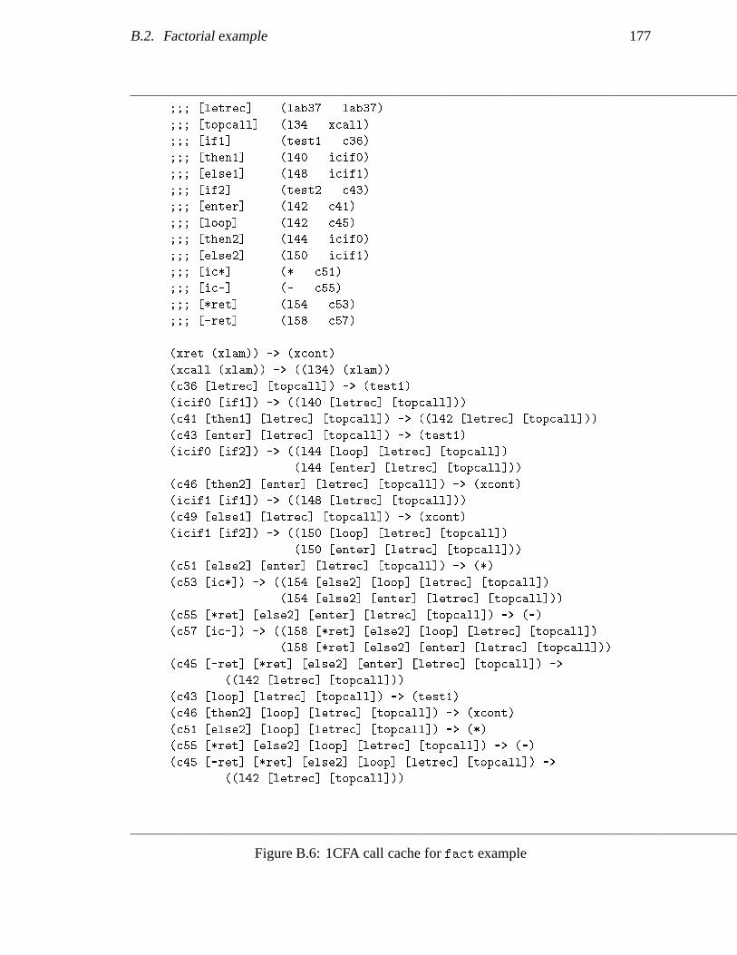
B.2. Factorial example 177
;;; [letrec] (lab37 . lab37)
;;; [topcall] (l34 . xcall)
;;; [if1] (test1 . c36)
;;; [then1] (l40 . icif0)
;;; [else1] (l48 . icif1)
;;; [if2] (test2 . c43)
;;; [enter] (l42 . c41)
;;; [loop] (l42 . c45)
;;; [then2] (l44 . icif0)
;;; [else2] (l50 . icif1)
;;; [ic*] (* . c51)
;;; [ic-] (- . c55)
;;; [*ret] (l54 . c53)
;;; [-ret] (l58 . c57)
(xret (xlam)) -> (xcont)
(xcall (xlam)) -> ((l34) (xlam))
(c36 [letrec] [topcall]) -> (test1)
(icif0 [if1]) -> ((l40 [letrec] [topcall]))
(c41 [then1] [letrec] [topcall]) -> ((l42 [letrec] [topcall]))
(c43 [enter] [letrec] [topcall]) -> (test1)
(icif0 [if2]) -> ((l44 [loop] [letrec] [topcall])
(l44 [enter] [letrec] [topcall]))
(c46 [then2] [enter] [letrec] [topcall]) -> (xcont)
(icif1 [if1]) -> ((l48 [letrec] [topcall]))
(c49 [else1] [letrec] [topcall]) -> (xcont)
(icif1 [if2]) -> ((l50 [loop] [letrec] [topcall])
(l50 [enter] [letrec] [topcall]))
(c51 [else2] [enter] [letrec] [topcall]) -> (*)
(c53 [ic*]) -> ((l54 [else2] [loop] [letrec] [topcall])
(l54 [else2] [enter] [letrec] [topcall]))
(c55 [*ret] [else2] [enter] [letrec] [topcall]) -> (-)
(c57 [ic-]) -> ((l58 [*ret] [else2] [loop] [letrec] [topcall])
(l58 [*ret] [else2] [enter] [letrec] [topcall]))
(c45 [-ret] [*ret] [else2] [enter] [letrec] [topcall]) ->
((l42 [letrec] [topcall]))
(c43 [loop] [letrec] [topcall]) -> (test1)
(c46 [then2] [loop] [letrec] [topcall]) -> (xcont)
(c51 [else2] [loop] [letrec] [topcall]) -> (*)
(c55 [*ret] [else2] [loop] [letrec] [topcall]) -> (-)
(c45 [-ret] [*ret] [else2] [loop] [letrec] [topcall]) ->
((l42 [letrec] [topcall]))
Figure B.6: 1CFA call cache for fact example

178 Appendix B. Analysis Examples

Bibliography
A book is a fat thing bound by itself, or the equiva-lent in some other medium of a fat thing bound byitself. A non-book is a thin thing or a thing that’spart of something else, or the equivalent in someother medium of a thin thing or a thing that’s partof something else.
— M-C. van Leunen
[Abramsky 87] Samson Abramsky and Chris Hankin (editors).Abstract Interpretation of Declarative Languages.Ellis Horwood, 1987.
[Aho+ 86] Alfred V. Aho, Ravi Sethi and Jeffrey D. Ullman.Compilers, Principles, Techniques and Tools.Addison-Wesley, 1986.
[Appel+ 89] Andrew W. Appel and Trevor Jim.Continuation-passing, closure-passing style.In Conference Record of the Sixteenth Annual ACM Symposium on Princi-
ples of Programming Languages, pages 293–302, January 1989.
[Berlin 89] Andrew A. Berlin.A compilation strategy for numerical programs based on partial evaluation.Master’s thesis, MIT, February 1989.
[Blelloch 90] Guy E. Blelloch.Vector Models for Data-Parallel Computing.MIT Press, 1990.
[Blelloch+ 90] Guy E. Blelloch and Gary W. Sabot.Compiling collection-oriented languages onto massively parallel comput-
ers.Journal of Parallel and Distributed Computing 8(2), February 1990.
179
180 Bibliography
[Bloss+ 86] Adrienne Bloss and Paul Hudak.Variations on strictness analysis.In Proceedings of the 1986 ACM Conference on Lisp and Functional
Programming, pages 132–142, August 1986.
[Brookes 89] Stephen Brookes.Course notes, graduate class on programming language semantics.School of Computer Science, CMU, 1989.These notes are currently being turned into a book.
[Chaitin 82] G. J. Chaitin.Register allocation & spilling via graph coloring.In Proceedings of the SIGPLAN ’82 Symposium on Compiler Construction,
published as SIGPLAN Notices 17(6), pages 98–105. Association forComputing Machinery, June 1982.
[Chaitin+ 81] G. J. Chaitin, et al.Register allocation via coloring.Computer Languages 6:47–57, 1981.
[Chow+ 84] Frederick Chow and John Hennessy.Register allocation by priority-based coloring.In Proceedings of the SIGPLAN ’84 Symposium on Compiler Construction,
published as SIGPLAN Notices 19(6), pages 222–232. Association forComputing Machinery, June 1984.
[Cousot 77] Patrick Cousot and Radhia Cousot.Abstract interpretation: a unified lattice model for static analysis of pro-
grams by construction or approximation of fixpoints.In Conference Record of the Fourth ACM Symposium on Principles of
Programming Languages, pages 238–252, 1977.
[Cousot 79] Patrick Cousot and Radhia Cousot.Systematic design of program analysis frameworks.Conference Record of the Sixth Annual ACM Symposium on Principles of
Programming Languages, pages 269–282, 1979.
[Curtis 90] Pavel Curtis.Constrained Quantification in Polymorphic Type Analysis.Ph.D. dissertation, Cornell University. Published as Xerox PARC Technical
Report CSL 90-1, February 1990.

Bibliography 181
[Deutsch 90] Alain Deutsch.On determining lifetime and aliasing of dynamically allocated data in
higher-order functional specifications (extended version).Research Report LIX/RR/90/11, LIX, Ecole Polytechnique, 91128 Palai-
seau Cedex, France.A conference-length version of this report appears in Conference Record
of the Seventeenth Annual ACM Symposium on Principles of Program-ming Languages, pages 157–168, January 1990.
[Ellis 86] John Ellis.Bulldog: A Compiler for VLIW Architectures.Ph.D. dissertation, Yale University. MIT Press, 1986.Also available as Research Report 364, Yale University, Department of
Computer Science.
[Fisher+ 84] Joseph A. Fisher, John R. Ellis, John C. Ruttenberg, and Alexandru Nico-lau.
Parallel processing: A smart compiler and a dumb machine.In Proceedings of the SIGPLAN ’84 Symposium on Compiler Construction,
published as SIGPLAN Notices 19(6), pages 37–47. Association forComputing Machinery, June 1984.
[Garner+ 88] R. Garner, et al.Scaleable processor architecture (SPARC).In COMPCON, pages 278–283. IEEE Computer Society, March 1988.
[Halfant+ 88] Mathew Halfant and Gerald Jay Sussman.Abstraction in numerical methods.In Proceedings of the 1988 ACM Conference on Lisp and Functional
Programming, pages 1–7, July 1988.
[Harrison 77] William H. Harrison.Compiler analysis of the value ranges for variables.IEEE Transactions on Software Engineering SE-3(3):243–250, May 1977.
[Harrison 89] Williams Ludwell Harrison III.The interprocedural analysis and automatic parallelization of Scheme pro-
grams.Lisp and Symbolic Computation 2(3/4):179–396, October 1989.
[Hecht 77] Matthew S. Hecht.Data Flow Analysis of Computer Programs.American Elsevier, New York, 1977.
182 Bibliography
[Hill+ 86] Mark Hill, et al.Design decisions in Spur.COMPUTER, 19(11):8–22, November 1986.
[Hudak 86] Paul Hudak.Collecting interpretations of expressions (preliminary version).Research Report 497, Yale University, Department of Computer Science,
August 1986.
[Hudak 86b] Paul Hudak.A semantic model of reference counting and its abstraction (detailed sum-
mary).In Proceedings of the 1986 ACM Conference on Lisp and Functional
Programming, pages 351–363, August 1986.
[Hudak+ 86b] Paul Hudak and Jonathan Young.Higher-order strictness analysis in untyped lambda calculus.In Conference Record of the Thirteenth Annual ACM Symposium on Prin-
ciples of Programming Languages, pages 97–109, January 1986.
[Johnston 71] John B. Johnston.The contour model of block structured processes.In Proceedings of a Symposium on Data Structures in Programming Lan-
guages, published as SIGPLAN Notices 6(2), pages 55–82. Associationfor Computing Machinery, February 1971.
[Kaplan+ 80] Marc A. Kaplan and Jeffrey D. Ullman.A scheme for the automatic inference of variable types.JACM 27(1):128–145, January 1980.
[Kelsey 89] Richard Kelsey.Compilation by Program Transformation.Ph.D. dissertation, Yale University, May 1989. Research Report 702, De-
partment of Computer Science.A conference-length version of this dissertation appears in POPL 89.
[Kranz 88] David Kranz.ORBIT: An Optimizing Compiler for Scheme.Ph.D. dissertation, Yale University, February 1988. Research Report 632,
Department of Computer Science.A conference-length version of this dissertation appears in SIGPLAN 86
[Kranz+ 86].
Bibliography 183
[Kranz+ 86] David Kranz, et al.ORBIT: An optimizing compiler for Scheme.In Proceedings of the SIGPLAN ’86 Symposium on Compiler Construction,
published as SIGPLAN Notices 21(7), pages 219–233. Association forComputing Machinery, July 1986.
[Kranz+ 89] David A. Kranz, Robert H. Halstead, Jr. and Eric Mohr.Mul-T: A high-performance parallel Lisp.In Proceedings of the SIGPLAN ’89 Conference on Programming Lan-
guage Design and Implementation, published as SIGPLAN Notices24(7), pages 81–90. Association for Computing Machinery, July 1989.
[Landin 64] Peter J. Landin.The mechanical evaluation of expressions.Volume 6, Computer Journal, January 1964.
[Lee 89] Peter Lee.Realistic Compiler Generation.Ph.D. dissertation, University of Michigan. MIT Press, 1989.
[Leroy 89] Xavier Leroy.Efficient data representation in polymorphic languages.In Programming Language Implementation and Logic Programming 90,
P. Deransart and J. Małuszynski (editors). Lecture Notes in ComputerScience, volume 456, Springer-Verlag 1990.
[Lucassen+ 88]John M. Lucassen and David K. Gifford.Polymorphic effect systems.In Conference Record of the Fifteenth Annual ACM Symposium on Princi-
ples of Programming Languages, pages 47–57, 1988.
[Milner 85] Robin Milner.The Standard ML core language.Polymorphism II(2), October 1985.Also ECS-LFCS-86-2, University of Edinburgh, Edinburgh, Scotland,
March 1986.
[Milner+ 90] Robin Milner, Mads Tofte and Robert Harper.The Definition of Standard ML.MIT Press, 1990.

184 Bibliography
[Moon 85] David A. Moon.Architecture of the Symbolics 3600.In proceedings of the 12th Annual International Symposium on Computer
Architecture, pages 76–83. IEEE Computer Society, June 1985.
[Mosses+ 86] Peter D. Mosses and David A. Watt.The use of action semantics.Technical Report DAIMI PB-217, Computer Science Department, Aarhus
University, Denmark.
[Mycroft 81] Alan Mycroft.Abstract Interpretation and Optimizing Transformations for Applicative
Programs.Ph.D. dissertation, University of Edinburgh, 1981.
[Pfenning+ 90]Frank Pfenning and Peter Lee.Metacircularity in the polymorphic lambda-calculus.To appear in Theoretical Computer Science.
[Pleban 81] Uwe Pleban.Preexecution Analysis Based on Denotational Semantics.Ph.D. dissertation, University of Kansas, May 1981.
[Rees+ 82] Jonathan A. Rees and Norman I. Adams IV.T: A dialect of Lisp or, Lambda: The ultimate software tool.In Conference Record of the 1982 ACM Symposium on LISP and Functional
Programming, pages 114–122, August 1982.
[Rees+ 84] Jonathan A. Rees, Norman I. Adams IV and James R. Meehan.The T Manual.4th edition, Yale University, Department of Computer Science, January
1984.
[Rees+ 86] J. Rees and W. Clinger (editors).The revised3 report on the algorithmic language Scheme.SIGPLAN Notices 21(12):37–79, December 1986.
[Reynolds 72] John C. Reynolds.Definitional interpreters for higher-order programming languages.In Proceedings of the ACM Annual Conference, pages 717–740, August
1972.

Bibliography 185
[Reynolds 78] John C. Reynolds.Syntactic control of interference.In Conference Record of the Fifth Annual ACM Symposium on Principles
of Programming Languages, pages 39–46, 1978.
[Riesbeck] Online documentation for the T3 implementation of the Yale loop packageis distributed by its current maintainer: Prof. Chris Riesbeck, YaleUniversity, Department of Computer Science. ([email protected]).
[Schmidt 86] David A. Schmidt.Denotational Semantics: a Methodology for Language Development.Allyn and Bacon, Boston, 1986.
[Sharir+ 81] Micha Sharir and Amir Pnueli.Two approaches to interprocedural data flow analysis.Chapter 7 of Program Flow Analysis: Theory and Applications, Steven
S. Muchnick and Neil D. Jones (editors), Prentice-Hall, 1981.
[Steele 76] Guy L. Steele Jr.Lambda: The ultimate declarative.AI Memo 379, MIT AI Lab, November 1976.
[Steele 78] Guy L. Steele Jr.RABBIT: A Compiler for SCHEME.Technical Report 474, MIT AI Lab, May 1978.
[Steele 90] Guy L. Steele Jr.Common Lisp: The Language.Digital Press, Maynard, Mass., second edition 1990.
[Steenkiste 87] Peter Steenkiste.Lisp on a Reduced-Instruction-Set Processor: Characterization and Opti-
mization.Ph.D. dissertation, Stanford University, March 1987. Technical Report
87-324, Computer Systems Laboratory.
[Stoy 77] Joseph E. Stoy.Denotational Semantics: The Scott-Strachey Approach to Programming
Language Theory.MIT Press, 1977.
[Tenenbaum 74]A. Tenenbaum.Type determination for very high level languages.Report NSO-3, Courant Institute of Mathematical Sciences, New York
University, 1974.

186 Bibliography
[Vegdahl+ 89] Steven R. Vegdahl and Uwe F. Pleban.The runtime environment for Screme, a Scheme implementation on the
88000.In ASPLOS-III Proceedings (Third International Conference on Architec-
tural Support for Programming Languages and Operating Systems),pages 172–182, April 1989. Proceedings published as simultaneousissue of SIGARCH Computer Architecture News 17(2), April 1989;SIGOPS Operating Systems Review 23(special issue), April 1989; andSIGPLAN Notices 24(special issue), May 1989. Association for Com-puting Machinery.
[Waters 82] Richard C. Waters.LETS: an expressional loop notation.AI Memo 680, MIT AI Lab, October 1982.
[Waters 89] Richard C. Waters.Optimization of series expressions, part I: User’s manual for the series
macro package.AI Memo 1082, MIT AI Lab, January 1989.
[Waters 89b] Richard C. Waters.Optimization of series expressions, part II: Overview of the theory and
implementation.AI Memo 1083, MIT AI Lab, January 1989.
[Wijngaarden 66]A. van Wijngaarden.Recursive definition of syntax and semantics.In the proceedings of the IFIP Working Conference on Formal Language
Description Languages, pages 13–24, 1964. Proceedings published asFormal Language Description Languages for Computer Programming,T. B. Steel, Jr. (editor). North-Holland, Amsterdam, 1966.
[Young+ 86] Jonathan Young and Paul Hudak.Finding fixpoints on function spaces.Research Report 505, Yale University, Department of Computer Science.
December 1986.