Control Engineering Perspective on Genome-Scale Metabolic Modeling

by

Andrew Louis Damiani

A dissertation submitted to the Graduate Faculty of

Auburn University

in partial fulfillment of the

requirements for the Degree of

Doctor of Philosophy

Auburn, Alabama

December 12, 2015

Key words: Scheffersomyces stipitis, Flux Balance Analysis, Genome-scale metabolic models,

System Identification Framework, Model Validation, Phenotype Phase Plane Analysis

Copyright 2015 by Andrew Damiani

Approved by

Jin Wang, Chair, Associate Professor of Chemical Engineering

Q. Peter He, Associate Professor of Chemical Engineering, Tuskegee University

Thomas W. Jeffries, Professor of Bacteriology, Emeritus; University of Wisconsin-Madison

Allan E. David, Assistant Professor of Chemical Engineering

Yoon Y. Lee, Professor of Chemical Engineering

ii

Abstract

Fossil fuels impart major problems on the global economy and have detrimental effects to

the environment, which has caused a world-wide initiative of producing renewable fuels.

Lignocellulosic bioethanol for renewable energy has recently gained attention, because it can

overcome the limitations that first generation biofuels impose. Nonetheless, in order to have this

process commercialized, the biological conversion of pentose sugars, mainly xylose, needs to be

improved. Scheffersomyces stipitis has a physiology that makes it a valuable candidate for

lignocellulosic bioethanol production, and lately has provided genes for designing recombinant

Saccharomyces cerevisiae.

In this study, a system biology approach was taken to understand the relationship of the

genotype to phenotype, whereby genome-scale metabolic models (GSMMs) are used in

conjunction with constraint-based modeling. The major restriction of GSMMs is having an

accurate methodology for validation and evaluation. This is due to the size and complexity of the

models. A new system identification based (SID-based) framework was established in order to

enable a knowledge-matching approach for GSMM validation. The SID framework provided an

avenue to extract the metabolic information embedded in a GSMM, through designed in silico

experiments, and model validation is done by matching the extracted knowledge with the

existing knowledge. Chapter 2 provides the methodology of the SID framework and illustrates

the usage through a simple metabolic network.

In Chapter 3, a comprehensive examination was carried out on two published GSMMs of

S. stipitis, iSS884 and iBB814, in order to find the superior model

iii

The conventional validation experiments proved to be unreliable, since iSS884 performed

better on the quantitative experiments, while iBB814 was better on the qualitative experiments.

The uncertainty of which model was superior was brought to light through the SID framework.

iBB814 showed that it agreed with the existing metabolic knowledge on S. stipitis better than

iSS884.

Chapter 4 showed that the errors in iBB814 were eliminated by refining iBB814 to

construct a modified model known as iAD828. The SID framework was used to guide model

refinement, which is typically a labor some and time intensive process. SID framework

eradicates the trial-and-error approach, but rather has the power to uncover the reaction errors.

iAD828 predicts xylitol production under oxygen-limited conditions, which is in agreement with

experimental reports. This was a significant improvement, since iSS884 and iBB814 does not

have this capability and now iAD828 can be used to properly engineer recombinant strains. Also

the SID framework results of iAD828 show noteworthy improvement relative to iSS884 and

iBB814.

The superior performance of iAD828 propelled the use of this model for strategies to

increase ethanol production. Understanding cofactor balance during fermentation is crucial in

obtaining high quality strains for ethanol overproduction. Recently much work has been done on

cofactor imbalance of the first two reactions of xylose metabolism-xylose reductase and xylitol

dehydrogenase. There is not a clear understanding in S. stipitis how the cofactor preference of

xylose reductase affects the metabolism. The cofactor preference of xylose reductase was varied

and an optimal phenotype was determined. Analysis from this guided in silico metabolic

engineering strategies resulted in elevated production of ethanol. This information can be found

in Chapter 5.

iv

In Chapter 6, SID enhanced PhPP analysis was developed as a tool to overcome the

limitations that PhPP analysis imposed. The power of this tool was shown by applying it to an

illustrated example and an E. coli core model. Here the traditional PhPP analysis was unable to

uncover the metabolic knowledge that the SID enhanced PhPP analysis was able to accomplish.

The traditional PhPP analysis used shadow prices to determine the different phenotypes. This

proved to be problematic for the E. coli core model. SID enhanced PhPP analysis was able to

detect a “missing” phenotype that PhPP analysis failed to uncover. Also as the size of the

metabolic model increases, the shadow price from PhPP analysis decreases to the point of having

only miniscule meaning. Error was shown in the shadow price of the formate exchange flux. SID

enhanced PhPP analysis provides a powerful tool for understanding metabolic phenotypes.

Chapter 7 describes the conclusions and the future work of this study.

v

Acknowledgments

First and foremost, I like to thank Jesus who gave me new life in Him, who called me out

of darkness and into the marvelous light while at Auburn. Thank you for the riches of grace and

patience to complete this work: 2 Corinthians 12:9 “My grace is sufficient for you, for My

strength is made perfect in weakness.”

I would like to express my appreciation for my advisor, Dr. Wang, for her persistent

support and her congenial concern throughout my graduate time. She is an exemplary mentor

and always takes the time to have a meeting for discussion. Dr. He, for his patience and support

when mentoring me on computational work and writing, awesome skills! Dr. Jeffries for his

valuable discussion and guidance, Dr. David for his thoughtfulness and asking challenging

questions, and to Dr. Lee and Dr. Goodwin for their support. I would also like to acknowledge

Dr. Ogunnaike, who encouraged me in applying for graduate school, and Dr. Eden for recruiting

me.

I would like to thank my group members: Hector Galicia, Meng Liang, Min Kim, Zi Xiu

Wang, Kyle Stone, Matthew Hillard, Devarshi Shah, Alyson Charles, Jeff Liu, Tomi Adekoya

and Rong Walburg for their support and valuable disscusions. Also I would like to thank the rest

of my fellow graduate students and staff at Auburn.

Special thanks to my parents, Andrew Damiani and Mary Jo Damiani, for their

sacrificing, love, and patience throughout the years. Also like to thank my sister and her brother-

in law, Melissa and Stephen Merced, and brother Nick for their love and support. Also to my

grandparents: Giselle and Vincent Damiani, and Ed and Carol Szumowski for their love and

encouragement. Also to my brothers and sisters in Christ who helped me get my footing in my

Christian walk. Jeff Cooling aka “the Guru” for his spiritual wisdom and guidance, and being an

vi

exemplary disciple of Jesus. Thanks to: Jeremy and AnneCatherine Crompton for their

friendship and encouragement, and to my church family at Fire and Grace Church. Thanks to:

Peter and Louis Morchen for our great discussions at Burger King. Thanks to: the prayer group

of Norma Stibbs for their love and unity, had many awesome times.

vii

Table of Contents

Abstract ............................................................................................................................... ii

List of Tables ..................................................................................................................... xi

List of Figures .................................................................................................................. xiii

Chapter 1. Introduction ....................................................................................................... 1

1.1 Renewable energy derived from biomass ................................................................. 1

1.1.1 Production of sustainable fuels .......................................................................... 1

1.1.2 Microbial strains for biofuels ............................................................................. 5

1.1.2.1 Saccharomyces cerevisiae ......................................................................... 5

1.1.2.2 Scheffersomyces stipitis ............................................................................. 7

1.1.2.2.1 Introduction .................................................................................... 7

1.1.2.2.2 Xylose metabolism .......................................................................... 8

1.1.2.2.3 Oxygenation characteristics ............................................................ 9

1.1.2.2.4 Electron Transport Chain (ETC) ................................................... 11

1.2 System biology ..................................................................................................... 11

1.2.1 Modeling of metabolic networks .................................................................. 13

1.2.2 Flux Balance Analysis (FBA) .......................................................................... 18

1.2.3 Genome-scale metabolic models (GSMMs) ................................................. 22

Chapter 2. System identification based framework .......................................................... 29

2.1 Introduction ............................................................................................................. 29

2.2 Procedure ................................................................................................................ 29

viii

2.3 Illustrative example ................................................................................................ 31

2.3.1 Case study 1: Objective function: maximal flux of re8 (production of D) ...... 33

2.3.2 Case study 2: Objective function: maximal flux of re9 (production of E)....... 34

Chapter 3. Comprehensive Evaluation of Two GSMMs for S. stipitis ............................. 37

3.1 Introduction ............................................................................................................. 37

3.2 Materials and Methods ........................................................................................... 38

3.2.1 Two published genome-scale models: iSS884 and iBB814 ............................ 38

3.2.2 In silico experiments ....................................................................................... 38

3.2.3 Phenotype phase plane (PhPP) analysis ........................................................... 39

3.2.4 Conventional point-matching using experimental data ................................... 39

3.2.5 System identification (SID) framework ........................................................... 40

3.2.6 Manual examination......................................................................................... 40

3.3 Results and Discussion ........................................................................................... 40

3.3.1 Model comparison using the existing methods ................................................ 42

3.3.1.1 Phenotype phase plane (PhPP) analysis .................................................. 42

3.3.1.2 Conventional point-matching using experimental data ........................... 44

3.3.1.3 Model comparison through the SID framework ..................................... 49

3.3.1.4 Manual examination guided by the SID framework ............................... 57

3.4 Conclusion .............................................................................................................. 63

Chapter 4. An improved GSMM for S. stipitis ................................................................. 65

4.1 Introduction ............................................................................................................. 65

4.2 Materials and Methods ........................................................................................... 67

4.2.1 Overview of GSMMs for S. stipitis ................................................................. 67

ix

4.2.2 SID framework ................................................................................................ 67

4.2.3 In silico examination and traditional experimental validation ......................... 74

4.3 Results and Discussion ........................................................................................... 75

4.3.1 Phenotype phase plane (PhPP) analysis ........................................................... 75

4.3.2 Model comparison through the SID framwork ................................................ 79

4.3.3 Validation experiments .................................................................................... 90

4.3.4 Redox analysis of iAD828 ............................................................................... 98

4.3.5 Limitations of iAD828 ................................................................................... 106

4.4 Conclusion ............................................................................................................ 106

Chapter 5. Cofactor engineering strategies for S. stipitis ............................................... 108

5.1 Introduction ........................................................................................................... 108

5.2 Materials and Methods ......................................................................................... 109

5.2.1 In silico experiments ...................................................................................... 109

5.2.2 SID framework............................................................................................... 109

5.3 Results and Discussion ......................................................................................... 110

5.3.1 Background of cofactor engineering of xylose reductase .............................. 110

5.3.2 Cofactor engineering of xylose reductase on iAD828 ................................... 111

5.3.3 Potential metabolic engineering strategies..................................................... 115

5.3.4 Switching the objective function to ethanol production rate ......................... 116

5.3.5 Metabolic engineering strategy 1 ................................................................... 116

5.3.6 Metabolic engineering strategy 2 ................................................................... 118

5.4 Conclusion ............................................................................................................ 120

Chapter 6. A System identificaiton Based Approach for Phenotype Phase Plane Analysis 121

x

6.1 Introduction ........................................................................................................... 121

6.2 Materials and Methods ......................................................................................... 123

6.2.1 Metabolic models ........................................................................................... 123

6.2.2 System identification enhanced PhPP analysis .............................................. 123

6.3 Results and Discussion ......................................................................................... 125

6.3.1 Illustrative Example ....................................................................................... 126

6.3.2 E. coli core model .......................................................................................... 136

6.4 Conclusion ............................................................................................................ 143

Chapter 7. Conclusion and Outlook ................................................................................ 145

7.1 Conclusion ........................................................................................................... 145

7.2 Outlook ................................................................................................................ 148

Bibliography ........................................................................................................... 150

Appendices .............................................................................................................. 167

xi

List of Tables

Table 1.1 Success of GSMMs for production of biofuels ............................................................ 26

Table 2.1 Internal and exchange reactions .................................................................................... 32

Table 3.1 The effects of inhibiting electron transport chain complexes on cell growth and

formation of AOX and Complex III or IV for glucose and xylose. .............................................. 47

Table 3.2 SID results of iSS884 and iBB814 under oxygen-limited condition ........................... 52

Table 3.3 Comparison of detailed fluxes through ETC in iSS884 and iBB814 under two different

OUR conditions ............................................................................................................................ 53

Table 3.4 Comparison of ethanol production routes in iSS884 and iBB814 ................................ 55

Table 3.5 SID results of iSS884 and iBB814 aerobic condition................................................... 56

Table 3.6 NADPH production pathways for iBB814 ................................................................... 56

Table 3.7 Amino acid production routes under oxygen-limited condition ................................... 59

Table 3.8 Metabolic artifacts that differ between iSS884 and iBB814 ........................................ 63

Table 4.1 Breakdown GSMMs of S. stipitis ................................................................................. 67

Table 4.2 Reactions that were modified in iAD828……………………………………………..71

Table 4.3 Reactions deleted from iAD828 ................................................................................... 73

Table 4.4 Reactions added to iAD828 .......................................................................................... 74

Table 4.5 Metabolic artifacts to further validate iAD828 ............................................................. 90

Table 4.6 The effects of inhibiting electron transport chain complexes on cell growth for glucose

and xylose………………………………………………………………………………………..96

Table 4.7 Comparison of iAD828 xylitol results to experimental data ........................................ 97

Table 4.8 Key redox reactions identified by SID framework for P17 ........................................ 100

xii

Table 4.9 Key redox reactions identified by SID framework for P16 ........................................ 101

Table 4.10 Key redox reactions identified by SID framework for P14 ...................................... 102

Table 4.11 Key redox reactions identified by SID framework for P10 ...................................... 104

Table 4.12 Key redox reactions identified by SID framework for LO ....................................... 105

Table 5.1 Reactions influenced by variation of XR ratio for P16 ............................................... 114

Table 6.1 Shadow prices of P1, LO, and P2 ............................................................................... 129

Table 6.2 Shadow prices of P3 and P4 ....................................................................................... 134

Table 6.3 Shadow prices of the substrates and products for all phenotypes for E. coli. ............ 141

Table 6.4 Shadow prices of the intermediate metabolites for all phenotypes for E. coli. .......... 141

xiii

List of Figures

Figure 1.1 Global production of hydrotreated vegetable oil, biodiesel, and bioethanol for 2000 -

2013................................................................................................................................................. 3

Figure 1.2 Xylose Metabolism of S. stipitis.. .................................................................................. 9

Figure 1.3 Outline of glucose and xylose metabolism in yeasts. .................................................. 10

Figure 1.4 ETC of S. stipitis.......................................................................................................... 11

Figure 1.5 Integrative approach of system biology ...................................................................... 13

Figure 1.6 Phylogenetic tree of constraint-based tools.. ............................................................... 17

Figure 1.7 FBA construction on a simplified metabolic network model. ..................................... 21

Figure 1.8 Plurality of levels for reconstruction of GSMM.......................................................... 24

Figure 1.9 Process for formulating high quality genome-scale models. ....................................... 26

Figure 1.10 Flow path of work of GsMNM for metabolic improvement of a desired compound…..28

Figure 2.1 System identification based framework ...................................................................... 31

Figure 2.2 Reaction network scheme…… .................................................................................... 32

Figure 2.3 Scaled PCA loading for case study 1. ......................................................................... 34

Figure 2.4 Visualization of the analysis results for case study 1 .................................................. 34

Figure 2.5 Scaled PCA loading for case study 2 .......................................................................... 35

Figure 2.6 Visualization of the analysis results for case study 2.. ................................................ 35

Figure 3.1 Phenotype phase plane analysis ................................................................................... 43

Figure 3.2 Model validation using experimental data from Caspeta et al. (2012) in which iSS884

was published…… ........................................................................................................................ 45

Figure 3.3 Model validation using experimental data from an independent source. .................... 46

Figure 3.4 Model comparison of the wild type vs. the mutant with the alternative route into the

pentose phosphate pathway for metabolizing xylose by deletion of xylulokinase reaction ......... 48

xiv

Figure 3.5 The SID framework identifies how fluxes are affected by the increased oxygen ....... 51

Figure 3.6 Visualization of the analysis results for case study 2.. ................................................ 54

Figure 3.7 Comparison of constituent reactions in iSS884 and iBB814…… .............................. 58

Figure 3.8 Reactions of the pyruvate metabolism linkage to TCA cycle. .................................... 60

Figure 4.1 Development of GSMMs for S. cerevisiae through the years ..................................... 66

Figure 4.2 Early rendition of iAD828 showing oxidative branch of PPP being not active …… . 68

Figure 4.3 Guided modification of SID framework. The direction of the oxidative branch of PPP

was corrected by SID framework. ................................................................................................ 69

Figure 4.4 Effect of RXm 7 on ethanol and acetic acid production for iAD828 .......................... 72

Figure 4.5 3D product profiles ...................................................................................................... 79

Figure 4.6 2D phenotype phase plots.. .......................................................................................... 80

Figure 4.7 Comparison of SID framework results for iSS884, iBB814, and iAD828 under

oxygen-limited condition…… ...................................................................................................... 83

Figure 4.8 SID framework results of P16 for iAD828.................................................................. 84

Figure 4.9 SID framework results of P14 for iAD828.................................................................. 85

Figure 4.10 Comparison of SID framework results under aerobic condition for iSS884, iBB814,

and iAD828.. ................................................................................................................................. 88

Figure 4.11 Line of optimality SID framework results of iBB814 and iAD828…… .................. 89

Figure 4.12 Figure 4.11 Line of optimality SID framework results of iBB814 and iAD828……93

Figure 4.13 Model validation using experimental data from Caspeta et al. (2012) in which

iSS884 was publisheddel validation using experimental data from an independent source. ........ 94

Figure 4.14 Model comparison of the mutant strains of iSS884, iBB814, and iAD828. ............. 95

Figure 4.15 Key redox reactions that were identified in P17 ....................................................... 99

Figure 4.16 Key redox reactions that were identified in P16 ..................................................... 101

Figure 4.17 Key redox reactions that were identified in P14…… ............................................. 102

xv

Figure 4.18 Key redox reactions that were identified in P10. .................................................... 103

Figure 4.19 Key redox reactions that were identified in LO. ..................................................... 105

Figure 5.1 Illustration of xylose metabolism in S. stipitis .......................................................... 111

Figure 5.2 Cofactor XR ratio influence on growth rate …… ..................................................... 112

Figure 5.3 Influence of cofactor preference of XR ratio under oxygen-limited condition. ........ 114

Figure 5.4 Metabolic engineering strategy 1 .............................................................................. 117

Figure 5.5 Metabolic engineering strategy 2 .............................................................................. 119

Figure 6.1 Example of PhPP analysis using genome-scale model iAD828. .............................. 122

Figure 6.2 Schematic diagram of SID enhanced PhPP analysis…… ......................................... 125

Figure 6.3 Illustrative example of network and reactions........................................................... 126

Figure 6.4 PhPP analysis of illustrative example ...................................................................... 127

Figure 6.5 Prediction of phenotypes using SID enhanced PhPP analysis. ................................. 128

Figure 6.6 Active and non-active reactions for P1, LO, and P2…… ......................................... 129

Figure 6.7 SID enhanced PhPP analysis for P1. ......................................................................... 131

Figure 6.8 SID enhanced PhPP for LO. ...................................................................................... 132

Figure 6.9 SID enhanced PhPP analysis for P2. ......................................................................... 133

Figure 6.10 Comparison of P1, LO, and P2. ............................................................................... 133

Figure 6.11 SID enhanced PhPP for P3. ..................................................................................... 134

Figure 6.12 SID enhanced PhPP for P4 ...................................................................................... 135

Figure 6.13 Central carbon metabolism of E. coli model. .......................................................... 136

Figure 6.14 Comparison of phenotypes from PhPP analysis and SID enhanced PhPP analysis. 137

Figure 6.15 SID enhanced PhPP analysis P3’ and P3’’. ............................................................. 138

xvi

Figure 6.16 Comparison of SID enhanced PhPP results of P3’ and P3’’-1. ............................... 138

Figure 6.17 Comparison of SID enhanced PhPP results of P3’ and P3’’-2 ................................ 139

Figure 6.18 Comparison of SID enhanced PhPP results of P2 and P4. ...................................... 140

Figure 6.19 Comparison of SID enhanced PhPP results of P4, P3’’, P3’, and P2 as oxygen pickup

is varied ....................................................................................................................................... 142

1

Chapter 1: Introduction

1.1 Renewable energy derived from biomass

Fossil fuels impose major worldwide economic concerns and environmental pressures,

due to there being a limited supply that needs to be able to foster an increasing energy

requirement of the industrialized world, and the adverse effects of the production of greenhouse

gases (Cherubini, 2010; Gupta and Verma, 2015). The strong dependency on petroleum based

fuels intensifies the problem, where it accounts for 80% of the energy needs and 73% of carbon

dioxide emissions worldwide. With the oil demand of world in 2013 being approximately 90

million barrels a day (Hufbauer and Charnovitz, 2009) and it is projected that in 2030 that it

reaches 116 million barrels a day, with the transportation sector accounting for 60% of this total.

Therefore there is an imperative mandate for alternative energy source (IEA, 2007). Using

biomass as an energy source to produce biofuels provides an attractive options in following

ways: (1) economic potential due to the increasing prices of fossil fuels, (2) provides a

sustainable source for energy in the future, and (3) affords favorable environmental conditions

due to no net carbon dioxide emissions and very low amount of sulfur (Balkema and Pols, 2015;

Eisentraut, 2010; Sobrino and Monroy, 2010).

1.1.1 Production of sustainable fuels

Bioethanol is the primary transportation fuel substitute for gasoline. It has many

favorable properties, one being that it comes from a renewable source and can be used as an

octane enhancer, since it is a high octane fuel. On the environment spectrum, it has low toxicity,

it is biodegradable, and minimal pollution is emitted. It also has the ability to diminish

greenhouse gas emissions, where it has been shown to decrease greenhouse gas compared to

2

fossil fuels 18% and 88% when using corn derived and cellulosic feedstock respectively

(Service, 2007). Also leading oil producing countries have a stronghold on importing countries,

thus blending bioethanol with gasoline provides a greater fuel security for countries. Another

benefit is that entirely new infrastructure is created that opens the doors for employment (Balat

and Balat, 2009; Evans, 1997). The last couple of decades have shown an increasing inclination

for bioethanol production with 31 billion liters in 2001 (Berg, 2001) to 39 billion liters in 2006

and it is projected to go to 100 billion liters in 2015 (Licht et al., 2006). The U.S. (United States)

is the leading producer, and the U.S. Department of Energy (DOE) and the U.S. Department of

Agriculture (USDA) have recently mandated that 36 billion gallons of biofuels be produced by

2022. The U.S. being the top producer in bioethanol is due to the strong governmental support,

which started back in 1978 with the Energy Tax Act that granted tax credits for ethanol usage.

Recently in 2007, congress passed the Energy Independence and Security Act, which mandated

the supply of 12 billion gallons of bioethanol by 2010 and this would increase to 15 billion

gallons for 2015. Figure 1.1 shows the production of biofuels, specifically hydrotreated

vegetable oil (HVO) known as “green diesel”, biodiesel, and bioethanol through the years of

2000 - 2013. Bioethanol remains the top biofuel being produced with 75% of the total biofuel

production, and U.S. production is around 50 billion liters, where almost all was from corn

feedstock. Brazil is the next largest producer; together the U.S. and Brazil produce 62% of the

bioethanol in the world, from sugar cane and corn. European countries are getting involved,

where the European Union has set similar goals as the U.S. (Cherubini, 2010).

3

Figure 1.1: Global production of hydrotreated vegetable oil, biodiesel, and bioethanol for 2000 –

2013 (Global Status Report - REN21, 2014)

1.1.1.1 First generation biofuels

First generation biofuels are produced from feedstocks that are derived from food crops.

Some of the commonly used raw materials are sugar cane, corn, animal fats, and vegetable oil

(Naik et al., 2007). Conventional methods are used for production of first generational

bioethanol, and production of first generation biofuels are considered a well-established industry.

Despite the need to reduce greenhouse gas emission, first generational biofuels provides limited

reduction (Collins, 2007). Another major drawback of first generation feedstocks is the

competition with the food industry (Marris, 2006).

1.1.1.2 Second generation biofuels

This has brought the incipient of second generation biofuels, which are based on nonfood

crops or crop resdiues. Unlike corn feedstock, which is composed of a starchy material,

ligonocellulosic biomass comes from the fibrous part of plant that is non-starchy. Lignocellulosic

4

biomass are divided into five groups of feedstocks: 1) agricultural residues (leftover material

from crops, such as corn stover and wheat straw); 2) forestry wastes (chips and sawdust from

lumber mills, dead trees, and tree branches); 3) municipal solid wastes (household garbage and

paper products); 4) food processing and other industrial wastes (black liquor, a paper

manufacturing by-product); and 5) energy crops (fast-growing trees and grasses, such as

switchgrass, poplar and willow) (Mansfield et al., 2006). Hexose and pentose sugars comprise

about 50 – 80% of the carbohydrates in lignocellulosic biomass. The carbohydrates are

biologically converted to bioethanol through fermentation (Mousdale, 2006). The carbohydrates

are broken down in two groups, cellulose and hemicellulose. Cellulose is composed of linear

glucose polymers that are β linked together. Hemicellulose is an extensive branched polymer

that is comprised of five-carbon sugars: arabinose and xylose, and a six-carbon sugar: galactose,

glucose, and mannose. There is a non-carbohydrate group, lignin, which provides the structural

foundation of the plant, where this part cannot be fermented (Sindu et al., 2015).

Lignocellulosic biomass is known as a green gold raw material, because it has many

advantages: (1) renewable and sustainable, (2) reduction of air pollutions that result from burning

and rotting of biomass in fields, (3) alleviating greenhouse gases, (4) provides economic benefits

locally through development and simulation, (5) halting energy dependence on countries that

rely on importing oil, and (6) generating technical jobs (Bjerre et al., 1996). It has been

calculated that lignocellulosic biomass has the potential to produce 442 billion liters of

bioethanol, which is due having the world’s largest renewable source of bioethanol (Hakeem,

2014). The two routes for conversion of lignocellulosic biomass to biofuels are done through

thermochemical and biochemical conversion. Thermochemical conversion first involves the

production of synthesis gas (blend of carbon monoxide and hydrogen) through gasification or

5

pyrolysis, then reformation of fuel through a catalytic process, such as the commonly used one of

the Fischer-Tropsch reaction or by a biological reaction. Biochemical conversion involves first

breaking down the sugar polymer to sugar monomers through pretreatment processing, and then

microorganisms are used to ferment the sugar into biofuels (Mckendry, 2002). A recent study

showed that production costs of second generation biofuels is two to three times more expensive

than petroleum based fuel production costs (Balan, 2014).

1.1.2 Microbial strains for biofuels

Present research efforts focus on fermenting glucose and xylose. Cofermentation is one

route that ferments the sugars simultaneously, and it is believed to have fewer costs then solely

fermenting the individual sugars (Ohgren et al., 2007; Zhao et al., 2008). There are a collection

of microorganisms available, such as Saccharomyces cerevisiae, Scheffersomyces stipitis,

Kluyveromyces marxianus, Candida shehatate, Zymomonas mobilis and Escherichia coli (Gírio

et al., 2010). Prokaryotes (E. coli) and lower eukaryotes are strains that have been used to

produce ethanol from biomass feedstocks. Yeast has enhanced properties, because they have

higher ethanol tolerance, resistance to contamination, growth at low pH, and have thicker cell

walls (Jeffries, 2006). Also yeast has already been in industrial applications, therefore there is an

established production facility (Hahn-Hägerdal et al., 2007).

1.1.2.1 Saccharomyces cerevisiae

S. cerevisiae is the most common microorganism used for ethanol production, which is

accomplished through fermentation of hexose sugars. When pentose sugars are present in the

feedstock the productivity diminishes. It has the capability only to metabolize phosphorylated

pentose sugars, like ribose 5-phosphate, but assimilation of pentoses such as xylose is

problematic. S. stipitis and E. coli can natively ferment xylose (Kim et al., 2007), however

6

ethanol productivity is still low so metabolic engineering to create recombinant strains, such as S.

cerevisiae or Z. mobilis has been a major focus on research (Joachimsthal and Rogers, 2000;

Martı́n et al., 2002; Jeppsson et al, 2002). The recombinant strains also have limitations, mainly

the one being a cofactor imbalance of the engineered pathway of the xylose metabolism, which

are xylose reductase and xylitol dehydrogenase (Roca et al., 2003; Matsushika et al, 2008;

Matsushika et al, 2009a). Another approach that has been used to bypass the cofactor imbalance

problem is to implement xylose isomerase; however most strains metabolized in this manner

have low xylose consumption rates (Van Maris et al, 2007; Kuyper et al, 2005; Karhumaa et al.,

2007). Other factors limiting xylose utilization in recombinant cells are inefficient xylose

transporters (Kötter and Ciriacy, 2003), lower capacity for the pentose phosphate pathway (PPP)

(Walfridsson et al, 1995) and inappropriate regulatory mechanisms (Jeffries and Van Vleet et al.,

2009). Efforts were made to increase the affinity of the xylose transporter. Sut1 increased ethanol

productivity; however capacity of the yeast was still limited (Katahira et al., 2008). Knowledge

of how yeasts such as S. stipitis natively ferment xylose is still limited in terms of relavant

biochemical reactions, thermodynamics, enzyme kinetics, and mechanistic understandings.

These factors all limit the extent to which could be the main reason that metabolic engineering

can succeed. Part of my research focuses on using genome-scale metabolic modeling of S. stipitis

to gain a better understanding of its cellular metabolism in order to understand which key steps

to change in order to improve both S. stipitis and engineered S. cerevisiae for lignocellulosic

ethanol production. Specifically, a genome-level understanding of xylose metabolism in S.

stipitis would help identify effective strategies for metabolic engineering design.

7

1.1.2.2 Scheffersomyces stipitis

1.1.2.2.1 Introduction

Scheffersomyces stipitis previously called Pichia stipitis that was first isolated from the

excreted frass of wood-ingesting beetles (Shi et al., 2002). Due to its important role in the

production of lignocellulosic ethanol, a second generation biofuel (Naik et al., 2010), S. stipitis

has drawn increasing research interest in the last few decades (Eisentraut, 2010). Currently

efficient pentose utilization remains one of the economic barriers to producing cost-effective

lignocellulosic ethanol through biological conversion (Margeot et al., 2009), and S. stipitis has

the highest native capacity to ferment xylose into ethanol (Van Dijken et al., 1986; Du Preez et

al., 1989). The concentration of ethanol can be up to 61 g/L in media containing xylose and

nutrients (Slininger et al., 2006). The ethanol yield spans between 0.31 – 0.48 g/g, which makes

this yeast strain one of the most effective for xylose fermentation for ethanol production

(Agbogbo and Coward-Kelly et al., 2008). Other reports that used a fed-batch setup were able to

produce up to 47 g/L of ethanol from xylose (Du Preez et al., 1989) with ethanol yields of 0.35 –

0.44 g/g (Hahn-Hägerdal and Pamment, 2004). With most of the carbon flux going toward

ethanol production, this leaves very little xylitol being produced. Nonetheless, fermentation rate

is still low on xylose when compared to glucose fermentation of S. cerevisiae.

It also has the capability to digest a spectrum of sugars that in are comprised in the

hydrolysate, such as glucose, galactose, mannose, and cellobiose. A recent study showed that S.

stipitis outperformed industrial strains in terms of fermentation (Matsushika et al., 2009b).

Under xylose fermentation conditions most of the carbon flux goes to ethanol production, while

a small amount goes to xylitol. The fermentation rate of glucose on S. cerevisiae is a lot higher

than xylose fermentation of S. stipitis. S. stipitis can produce ethanol at a yield close to the

8

theoretical maximum under oxygen-limitation. In addition, low ethanol tolerance and no growth

under anaerobic condition are also limitations that complicate utilization in industrial

applications. (Du Preez et al., 1989; Grootjen et al., 1990; Shi & Jeffries, 1998). To address these

limitations, attempts have been made to improve the xylose uptake rate of S. stipitis under

oxygen-limitation, as well as to introduce enzymes for the xylose fermentation pathways from S.

stipitis into engineered S. cerevisiae (Johansson & Hahn-Hagerdal, 2002; Karhumaa et al.,

2005). Many metabolic engineering and adaptive evolution strategies that been used with S.

cerevisiae (Harhangi et al., 2003; Sonderegger et al., 2004). However, these attempts have not

been entirely successful (Kotter & Ciriacy, 1993; Eliasson et al., 2000; De Deken, 1966;

Bruinenberg, et al. 1983), which is due redox balance, lack of sugar transports and digestion

genes. It is important to gain further understanding to either improve it as a host strain or even as

a gene provider for other strains.

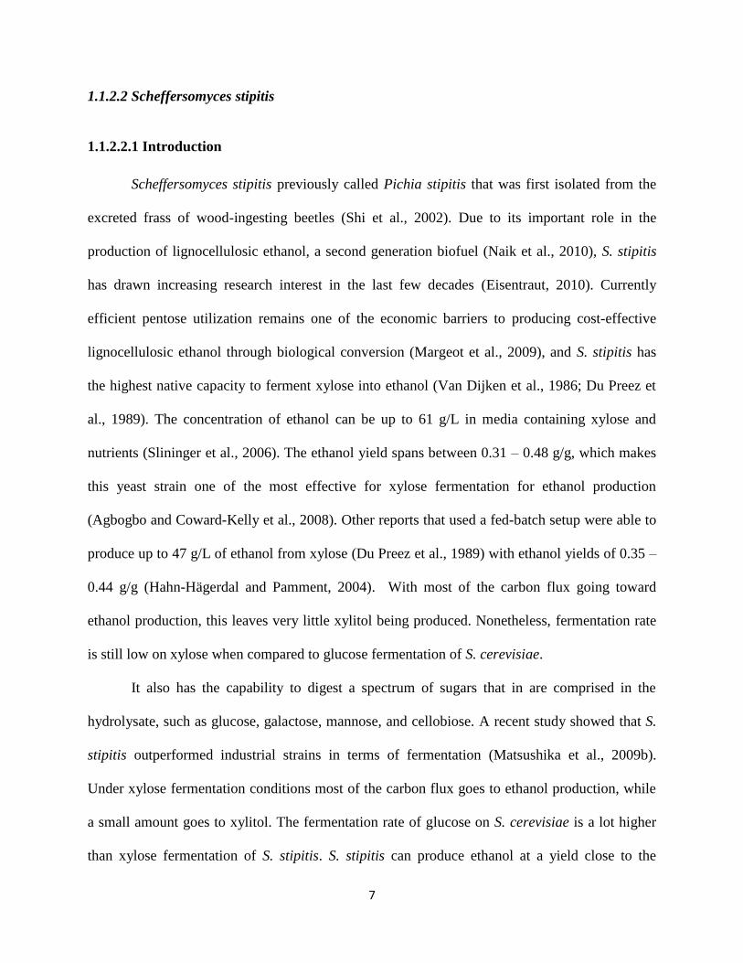
1.1.2.2.2 Xylose metabolism

Figure 1.2 shows the xylose metabolism for S. stipitis, where xylose is converted into

xylitol by a xylose reductase (XR), that has the ability to use both NADH and NADPH with an

activity ratio of 0.7 for NADH/NADPH (Jeffries et al., 1999). Xylitol is then oxidized to

xylulose by xylitol dehydrogenase (XDH), where NAD is used as the cofactor. NADP is given a

dashed line, since there have been reports that this cofactor has also been used for this reaction

(Matsushika et al., 2008; Yablochkova et al., 2004). Xylulose is phosphorylated to xylulose 5-

phosphate, which then enters the non-oxidative branch of PPP. The end products of the non-

oxidative branch of PPP is carbon compounds of fructose 6-phosphate and glyceraldehyde 3-

phosphate (Jeffries, 2006).

9

Figure 1.2: Xylose Metabolism of S. stipitis. Red letters without parenthesis represent enzymes.

Red letters in parenthesis represent genes that encode the enzymes

Diauxic behavior is shown for S. stipitis, when glucose and xylose are incorporated into

the same media (Grootjen et al., 1991; Slininger et al., 2011). Gene expression data showed that

Xyl1, Xyl2, and Xyl3 were upregulated for both oxygen-limited and aerobic conditions, when

xylose was used as the substrate, but these genes where downregulated when glucose was used

(Jeffries et al., 2007). When Xyl1 expression was increased (Takuma et al., 1991) this resulted in

enzymatic activity increasing two-fold, however this had no profit for ethanol production (Dahn,

et al., 1996).

1.1.2.2.3 Oxygenation characteristics

S. stipitis is a Crabtree-negative yeast, meaning that the presence or abesnce of oxygen

regulates the fermentation rate, as opposed to the Crabtree-positive yeast (S. cerevisiae), where

fermentation is regulated by the level of the sugar concentration present, such as glucose, making

it independent of oxygen uptake rate. Respiro-fermentative behavior is seen only under oxygen-

limited condition for S. stipitis (Klinner et al., 2005). Under oxygen-limitation, the enzymes

pyruvate decarboxylase and alcohol dehydrogenase show increased activity (Skoog and Hahn-

Hägerdal, 1990; Skoog et al., 1992) as well as their corresponding genes (Jeffries et al., 2007).

These are the enzymes that catalyze reactions for ethanol production, where pyruvate

decarboxylase (Pdc1 and Pdc5) and alcohol dehydrogenase (Adh1 and Adh2) are shown in

Figure 1.3. Alcohol dehydrogenase (Adh1) was ten times higher under oxygen-limited than

10

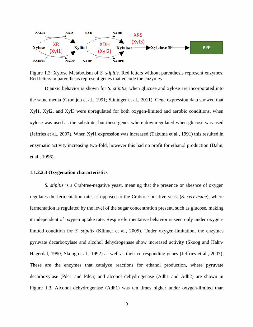
aerobic conditions. Also pyruvate decarboxylase was activated when oxygen levels switched

from aerobic to oxygen-limited condition (Cho and Jeffries, 1999).

Figure 1.3: Outline of glucose and xylose metabolism in yeasts. Enzyme designations are from

assigned loci in Saccharomyces cerevisiae or Pichia stipitis. Hxk1 Hexokinase P1; Hxk2

hexokinase PII; Glk glucokinase; Pgi phosphoglucose isomerase; Pfk phosphofructokinase 1;

Fbafructose-bisphosphate aldolase; Tdh (G3p) glyceraldehyde-3-phosphate dehydrogenase; Pgk

3-phosphoglycerate kinase; Gpm phosphoglycerate mutase; Eno enolase (2 phosphoglycerate

dehydratase); Pyk pyruvate kinase; Pdc pyruvate decarboxylase; Adh alcohol dehydrogenase;

Pdh pyruvate dehydrogenase; Dha aldehyde dehydrogenase; Acs acety l-coenzyme A synthetase;

6Pg 6-phosphogluconate dehydrogenase, decarboxylating; Rpe ribulose-phosphate

3-epimerase; Rki ribose-5-phosphate isomerase; Tkl transketolase; Tal transaldolase; Xor

xylose (aldose) reductase; Xid xylitol dehydrogenase; Xks xylulokinase (Jeffries and Shi, 1999)

One major disadvantage of S. stipitis is its inability to grow even though it can produce

ethanol under anaerobic conditions (Bruinenberg et al., 1994). It is still unclear why S. stipitis

cannot grow under anaerobically it needs only minimal oxygen present to achieve optimal

ethanol production conditions (Cho and Jeffries, 1999).

11

1.1.2.2.4 Electron Transport Chain (ETC)

S. stipitis has the standard respiration machinery along with alternative respiratory

components that allow the transfer of electron transfer to occur with or without coupling to ATP

production. This allows electrons either to enter through Complex I for mitochondrial NADH

oxidation or through the external or internal non-proton translocases of NADH or NADPH. A

clear depiction of this can be seen in Figure 1.4. At the terminal of the ETC is Complex IV,

which is part of the standard machinery or an alternative oxidase, which can be used under very

low oxygen conditions and only on xylose not glucose.

Figure 1.4: ETC of S. stipitis. Contains the proton-translocating NADH dehydrogenase

(Complex I); internal and external non-proton translocating NADH dehydrogenase (NADHIN,

NADHEX);internal and external non-proton translocating NADPH dehydrogenase (NADPHIN,

NADPHEX); succinate dehydrogenase (Complex II); ubiquinone complex (CoQ); SHAM-

sensitive alternative terminal oxidase, cytochrome bc1 (Complex III); cytochrome c (Cyt c); and

cytochrome c oxidase (Complex IV) (Joseph‐Horne et al., 2004)

1.2 System biology

System biology is a rapidly growing field of study that was primary developed in

academia, and is gaining popularity in commercial industries (Ideker et al., 2001). Biological

systems present a great challenge to researchers due to the great complexity. Conventionally,

scientists have adopted the reductionist point of view, which states that examining the simplest

parts of a system are critical in understanding the system as a whole. The system is broken down

12

to the most reduced state of complexity, and then worked upward in complexity. This separates

biological systems into specific parts, and then studies them under isolation (Aderem, 2005;

Gallagher et al., 1999). Then once all the parts are understood, then the pieces can put together

like a puzzle and the understanding of the system can be established. Scientists have devoted

their lives to study one particular gene or protein in order to gain knowledge. Although success

has been achieved using the reductionist approach, however when applied to biological system

there are great limitations, such that it is a grueling process that makes it pretty much impossible

to unravel the mechanisms involved. This is mainly due to gaining a higher level of

understanding the interactions between genes, proteins, and their effect on the metabolism. The

development of innovative technologies has brought about the production of complex biological

datasets. Genetic synthesis technologies and sequencing has emerged in biological research that

have reaped the sequencing the first genome and genome-scale metabolic models. System

biology provides a comprehensive functionality of biological systems through studying the

behavior and relationship of the biological elements simultaneously (Barabasi et al., 2004).

Mainly it utilizes a holistic approach from which quantitative data can be extracted. Rather than

examining an individual biological entity, it allows for studying the flow of information as a

whole on all biological levels, such as on proteins, genomics, regulation networks, and

metabolically (Spencer et al., 2008; Tang et al., 2005; Palsson, 2002). Figure 1.5 provides the

general concept of system biology versus the traditional reductionist approach. The reductionist

approach investigates the individual components of a system, such as the components of a

computer network or genes of a specific organ. System biologists integrate information together

globally, therefore instead of performing their research to the far left as the reductionist, their

research proceeds to the right, where the whole system can be studied together (Galitski, 2012).

13

Figure 1.5: Integrative approach of system biology (Galitski, 2012)

A recent paper (Sauer et al., 2007) stressed on the significance of using a system-level approach

for studying cellular metabolisms: “Rather than a reductionist viewpoint (that is, a deterministic

genetic view), the pluralism of cause and effects in biological networks is better addressed by

observing, through quantitative measures, multiple components simultaneously, and by rigorous

data integration with mathematical models. Such a system-wide perspective (so-called systems

biology) on component interactions is required so that network properties, such as a particular

functional state or robustness, can be quantitatively understood and rationally manipulated”.

My work used an integrative perspective by comparing, refining, and validating genome-

scale metabolic network models in order to gain a systems level understanding. Let us now look

at the literatue of the modeling techniques that were employed.

1.2.1 Modeling of metabolic networks

The primary goal of modeling metabolic networks is to deconstruct the complex

information of the microorganism into a computational framework with the objective of

predicting the cellular phenotype from the genotype (Bordbar et al., 2014). Compared to other

biological systems, metabolic networks are relatively well understood, which is attributed to

14

knowledge of the metabolites and the reactions that convert the biological constituents. The

structure of the metabolic reactions and their connectivity is established, thus we have a

fundamental understanding of the metabolic network. Metabolism is a key player for regulating

the homeostasis of organisms, because of the constant substrate being taken up and conversion

into building blocks for biomass and by-products. The size of metabolic networks is typically

classified under two camps: central carbon metabolism models (~80 reactions, 40 metabolites)

and genome-scale models (>1000 reactions, >500 metabolites) (Krömer et al., 2014).

Commonly, there are four primary approaches are taken to model metabolic networks (Stelling,

2004; Zomorrodi et al., 2012): 1. Interaction-based networks – neglect the stoichiometry of the

network and emphasize the network connectivity. The main assumption is that the system

remains stationary. Are used in large-scale systems (transcription of genes and proteomics) that

focus on how information is propagated. 2. Dynamic models – ordinary differential equations

with kinetic information are used to depict the dynamics of the system. 3. Stoichiometric models

– examine fundamental cellular biochemistry that is used to quantify the intracellular mass flow

at steady state, where the system is used to be stationary. 4. Stoichiometric models with kinetic

information – very similar to type 3 (Stoichiometric models) except now there exists at least one

kinetic equation that relates the concentration of a metabolite to the reaction rate.

Modeling that is done in biological systems usually invokes theory-based models, which

involves a particular input with a set equation for a specific solution. These types of models are

troublesome, because the kinetic parameters need to be determined through expensive

experiments (Famili et al., 2005; Segrè et al., 2003). The accurate determination of the

parameters can be often questioned, due to the variability and difficulty of their measurements.

Parameters need to be quantified usually have significant error or have not even been measured

15

under in vivo conditions (Rizzi et al., 1997; Teusink et al, 2000; Vaseghi et al., 1999; Wright and

Kelly, 1981). Due to these shortcomings, there has been no genome-scale theory-based model

constructed (Jamshidi and Palsson, 2008). Another common approach is cybernetic modeling,

which finds unknown or hidden parameters through various assumptions (Kompala et al, 1984;

Young et al, 2008).

Constraint-based models are known as structural metabolic network modeling, which

does not require kinetic parameters, but rather defined constraints. They are based on the micro-

evolutionary principle that biological systems have adapted to diverse environments over time

and as they multiply they are not identical to their parent cells. Palsson describes the phenomena

this way: “To survive in a given environment, organisms must satisfy myriad constraints, which

limit the range of available phenotypes. All expressed phenotypes resulting from the selection

process must satisfy the governing constraints. Therefore, clear identification and statement of

constraints to define ranges of allowable phenotypic states provides a fundamental approach to

understanding biological systems that is consistent with our understanding of the way in which

organisms operate and evolve (Palsson et al, 2006)”. Constraint-based models have been around

for more than 25 years, since 1986 (Fell and Small, 1986), peaking in the mid-1990’s (Savinell

and Palsson et al, 1992; Varma et al., 1993) they were used to compute the metabolic flux

distribution and cellular growth.

The different types and magnitudes of the constraints will limit the cellular function. A

recent paper summarizes the types of constraints in four categories: fundamental physico-

chemical constraints, topological constraints, environmental constraints, and regulatory

constraints.

16

(i) Physico-chemical constraints: Numerous constraints govern cellular metabolism

and are known as hard constraints. Hard constraints are the laws of conservation

of mass, energy, and thermodynamics (Covert et al, 2001; Edwards et al., 2002).

These constraints will not change with the environmental pressures.

(ii) Topological constraints: This deals with the crowding of molecules inside the cell.

For instance, the length of a bacterial genome is on the magnitude of 1000 times

the length of the cell. Thus this means that the DNA must be crammed tightly, but

fully accessible in order to be unraveled into cellular machinery.

(iii) Environmental constraints: These constraints are time and condition dependent.

Examples of these constraints are availability of nutrients, pH, temperature, and

osmolality

(iv) Regulatory constraints: These constraints are different from the three types

described above, because they are self-imposed constraints. They can change

based on the evolutionary conditions and can vary with time. These constraints

are used to eradicate suboptimal phenotype states and improve fitness. Recently,

there are regulatory constraints based on transcriptional levels of genes (Reed et

al., 2012).

17

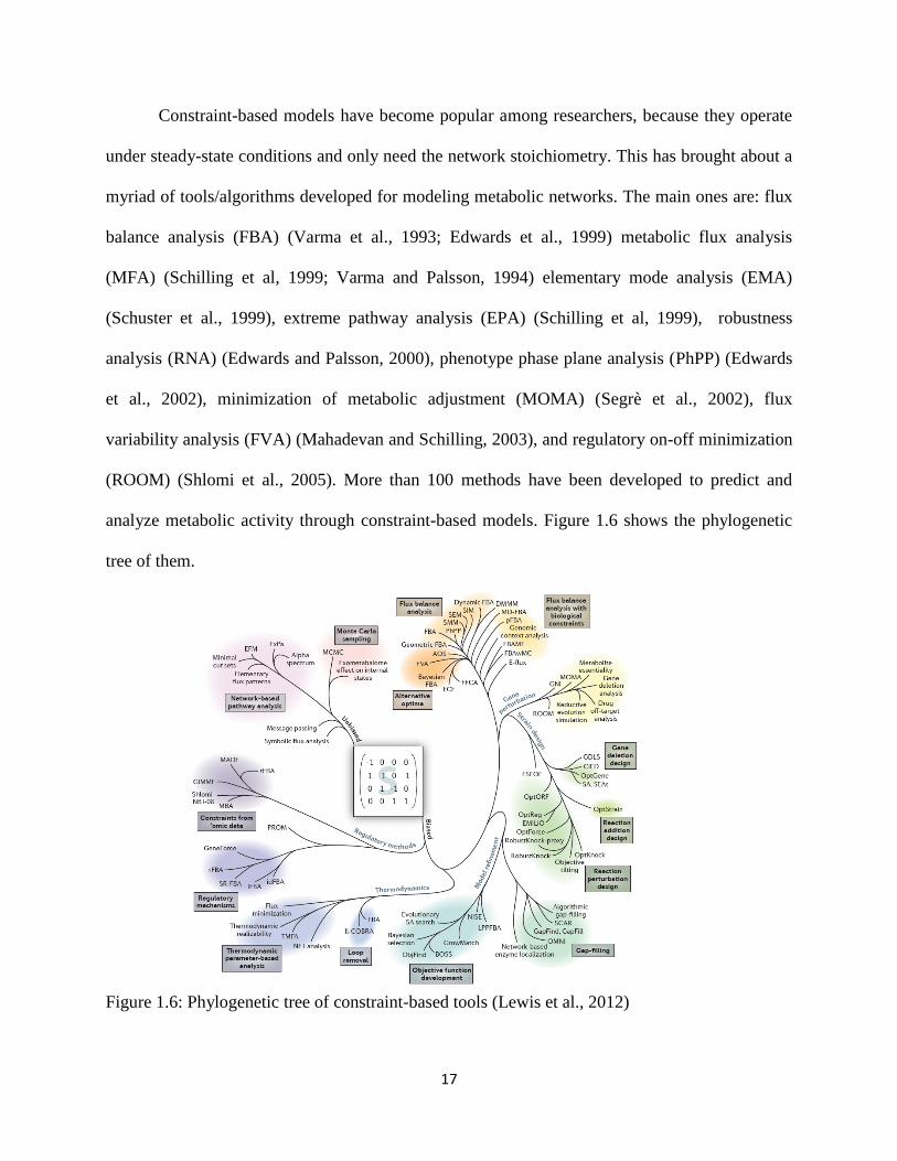
Constraint-based models have become popular among researchers, because they operate

under steady-state conditions and only need the network stoichiometry. This has brought about a

myriad of tools/algorithms developed for modeling metabolic networks. The main ones are: flux

balance analysis (FBA) (Varma et al., 1993; Edwards et al., 1999) metabolic flux analysis

(MFA) (Schilling et al, 1999; Varma and Palsson, 1994) elementary mode analysis (EMA)

(Schuster et al., 1999), extreme pathway analysis (EPA) (Schilling et al, 1999), robustness

analysis (RNA) (Edwards and Palsson, 2000), phenotype phase plane analysis (PhPP) (Edwards

et al., 2002), minimization of metabolic adjustment (MOMA) (Segrè et al., 2002), flux

variability analysis (FVA) (Mahadevan and Schilling, 2003), and regulatory on-off minimization

(ROOM) (Shlomi et al., 2005). More than 100 methods have been developed to predict and

analyze metabolic activity through constraint-based models. Figure 1.6 shows the phylogenetic

tree of them.

Figure 1.6: Phylogenetic tree of constraint-based tools (Lewis et al., 2012)

18

Modeling techniques discussed above compute static metabolic states. However, there

are disadvantages: the cell’s dynamic behavior cannot be determined, there are difficulties on

implementing cellular regulation, and most experiments are done in batch and fed-batch cultures,

where a dynamic model is required (Antoniewicz, 2013; Kauffman et al., 2003). Presently, the

dynamic behavior is modeled through three modeling techniques, which are kinetic modeling,

cybernetics, and dynamic FBA. For kinetic modeling and cybernetics require parameters that

need to be fitted through designed experiments (Raman and Chandra, 2009; Smallbone et al.,

2010). Dynamic FBA is an extension of FBA, however it does require empirical substrate

equations, such as using michaelis-menten kinetics (Hanly and Henson, 2011; Hjersted and

Henson, 2009). Dynamic modeling is not examined in this work, but is a future step that is

needed to improve model prediction.

1.2.2 Flux Balance Analysis

Flux balance analysis (FBA) is a powerful technique that was developed in 1993 (Varma

and Palsson, 1993). It was the first optimization-based tool for determining the metabolic flux

distribution (Varma and Palsson, 1994). The metabolic network is treated as a linear

programming problem, and an objective function, typically growth rate, is used to calculate an

optimal solution. Reversibility data for reactions are used for the lower and upper bounds in

order to constrain the reaction fluxes, which are the variables in the problem. The other

constraints are the extracellular uptake rates of the substrates, such as carbon and oxygen source.

This method is used calculate the flow of metabolites in a metabolic network, metabolite of

interest (Orth et al., 2010). There are currently more than 35 organisms that have metabolic

network models developed, and high-throughput technologies allow the construction of many

19

more each year, thus FBA is extremely important tool for gaining biological knowledge in these

models (Gianchandan et al, 2010; Orth et al, 2011; Schellenberger et al., 2011).

As previously discussed, FBA doesn’t require kinetic parameters, but it uses well defined

constraints based on fundamental laws of nature. However, there are limitations to this, such that

it does not calculate metabolite concentration (Lee et al., 2006). Also the focus is solely on the

metabolism, so it does not incorporate regulatory effects of genes or enzyme activity

(Ramakrishna et al, 2001). Because it is a steady-state approach, it only uses time-invariant

substrate and nutrient consumption rates, thus it is only uses prediction from continuous

experiments.

A simplified metabolic network model of 4 reactions and 3 metabolites is displayed in

Figure 1.7 to demonstrate how FBA is carried out. This can be thought of a network flow

problem in the field linear programming, where the metabolites are nodes and the reactions are

the edges. The next section will discuss how genome-scale metabolic network models are

construction, but briefly these are generated from an annotated genome and other biochemical

and physiological databases. The reconstruction process is extensive, such that it can take

months or years to complete (Thiele and Palsson, 2010; Henry, et al., 2010). A mass balance is

prescribed on each metabolite in the network and is written in the form of a stoichiometric matrix

(S). The rows and columns represent each unique reaction and metabolite, respectively. Each

column entry represents the stoichiometric coefficient of each metabolite. The sign determines

whether a metabolite is consumed or produced, a positive sign is production and a negative sign

is consumption. If the metabolite is not present in the reaction the entry receives a zero. The

stoichiometric matrix is mass balanced, meaning the total consumption and production each

metabolite is balanced at steady state. It is common for the reactions to exceed the number of

20

metabolites. This becomes an underdetermined problem, meaning that there is infinite number of

solutions. Here the key assumption of a steady state system is made which transforms this from a

dynamic problem into a static one. This assumption is justified the assumptions that (1)

intracellular metabolites reach thermodynamic equilibrium orders of magnitude faster than

enzyme level change or cells double, and (2) in constrast to metabolite flux, intracellular

metabolite concentrations change minimally in response to physiological changes in the cell

because they are largely determined by enzyme affinities rather than reaction rates. As a result,

metabolite levels are balanced kinetically and thermodynamically at each flux. The x term

represents the metabolite concentration, where this is shown in the derivative with respect to

time, and the v is the matrix of fluxes of individual reactions combined. FBA lessens the

computational load by assuming a steady state, where, such is turned into a time-invariant

problem, which is essentially like solving for the null space.

Using the assumption of a steady state is a generally acceptable practice in systems

biology, which eliminates the convoluted system dynamics of metabolism that takes into

consideration the kinetics and enzyme activities. As stated above the justification stems from the

fact that the metabolite levels are highly transient relative to the cellular growth and the

extracellular environmental changes. Studies showed that the metabolic transients only last a

couple of minutes, therefore the metabolic fluxes are in a quasi-steady state in comparison to the

growth and process transients (Varma and Palsson, 2004).

From there the reactions are constrained, that are primarly in the pickup and output

reactions, such as substrates, oxygen, and byproducts. Intracellular reactions can be constrained

if there is supporting experiment information, such as through 13

C labeled experiments of the

metabolic flux (Sauer, 2006; Wiechert, 2001). The variable vi represents an individual reaction,

21

where it is constrained between a lower bound αi and an upper bound βi. Implementation of

constraints generates a solution space of an n dimensional polytope, which is the allowable

solution space of flux distributions. Ingrafting constraints is why researchers have named this

approach, constraint-based metabolic models (Llaneras and Picó, 2010).

The final step is to determine an objective function in order to pinpoint a unique solution

in the feasible space of the polytope. In the early years of FBA, there were many objective

functions selected (Pramanik and Keasling, 1997; Varma and Palsson, 1994), however then the

maximization of the biomass objective function emerged as the main one, which it is the

stoichiometric yield for biomass. It is contains in equation format the building blocks that make

up the biomass component. It has been determined that flux through the biomass reaction rate is

directly proportional to the growth of the organism (Stephanopoulos et al., 1998). The micro-

evolution principle is applied, which states that surviving microorganisms have gained an

advantage over the competing microorganisms by growing in more of an effective way.

Therefore optimization guides cellular decision making.

Figure 1.7: FBA construction on a simplified metabolic network model (Patiño et al., 2012)

22

The biomass growth reaction is based on experimentally determined biomass components

(Feist et al., 2010; Schuetz et al., 2007). Other maximization objective functions are metabolite

synthesis (Montagud et al., 2010) and a plural objective scheme of biomass and metabolite

synthesis (Burgard et al., 2003; Pharkya et al, 2004). In constrast, the minimization objective

functions are: redox power, (Knorr et al., 2007), ATP formulation (Knorr et al., 2007; Vo et al.,

2004), and nutrient uptake (Segrè et al., 2002).

There are numerous of software tools that carry out FBA, such as the COBRA toolbox

(Becker et al., 2007) that is coded in Matlab. Others are Pathway tools (Paley et al., 2012),

BioMet toolbox (online usage) (Cvijovic et al., 2010) and OptGene (offline usage) (Patil et al.,

2005; Rocha et al., 2008)

1.2.3 Genome-scale metabolic models (GSMMs)

Genome-scale metabolic models (GSMMs) provide a relationship between the genotype

and phenotype; they provide a holistic view of the cellular metabolism. Once validated, GSMMs

provide a platform to effectively interrogate cellular metabolism, such as characterizing

metabolic resource allocation, predicting phenotype, and designing experiments to verify model

predictions, as well as designing mutant strains with desired properties (Liu et al., 2010;

Oberhardt et al., 2009). More importantly, GSMMs allow systematic assessment of how a

genetic or environmental perturbation would affect the organism as a whole (Becker et al.,

2007).

GSMMs were developed in the 1990’s due to the emergence of sequencing whole

genomes (Schilling et al., 1999). The first GSMMs were achieved in the organism of bacteria for

H. influenza (Schilling and Palsson, 2000) and E. coli (Edwards and Palsson, 2000). However,

there were metabolic models before this, starting with Fell and Small (1986), Mavrovouniotis

23

and Stephanopoulos (1992), and Savinell and Palsson (1992), however these models did not

contain all the reactions in the genome due to the lack of sequencing technology. The price of

sequencing entire genomes has been reduced in recent years, and this has opened the door for

metabolic reconstructions (Henry et al., 2010).

Developing a reliable GSMM is comprised in four steps: (1) network reconstruction, (2)

manual curation and building mathematical model, (3) model validation using experimental data,

and (4) refinement of the model by iterations between computational and experimental parts. An

annotated genome must be supplied to reconstruct a GSMM. Genes account for metabolic

functions and draft reconstructions are constructed, which tell us the relationship between genes,

reactions, and metabolites.

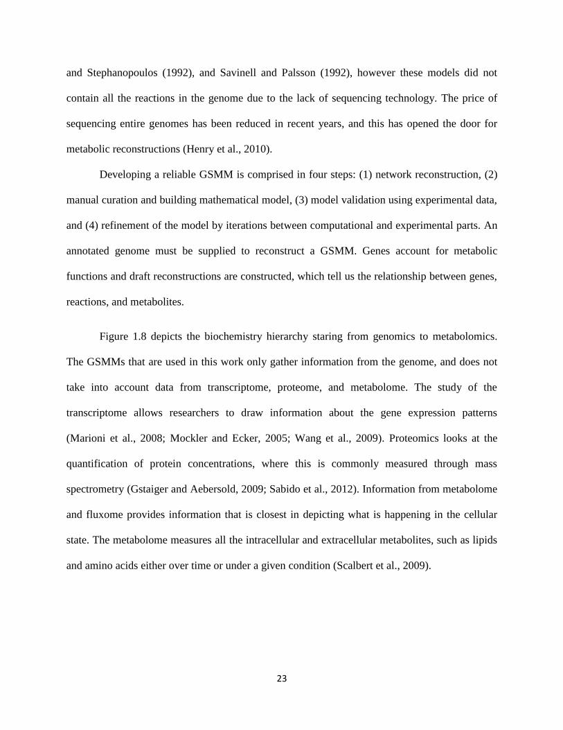
Figure 1.8 depicts the biochemistry hierarchy staring from genomics to metabolomics.

The GSMMs that are used in this work only gather information from the genome, and does not

take into account data from transcriptome, proteome, and metabolome. The study of the

transcriptome allows researchers to draw information about the gene expression patterns

(Marioni et al., 2008; Mockler and Ecker, 2005; Wang et al., 2009). Proteomics looks at the

quantification of protein concentrations, where this is commonly measured through mass

spectrometry (Gstaiger and Aebersold, 2009; Sabido et al., 2012). Information from metabolome

and fluxome provides information that is closest in depicting what is happening in the cellular

state. The metabolome measures all the intracellular and extracellular metabolites, such as lipids

and amino acids either over time or under a given condition (Scalbert et al., 2009).

24

Figure 1.8: Plurality of levels for reconstruction of GSMM (Nemutlu et al., 2012)

Fluxomics provides the rate of metabolic reactions at the scale of the network. Again mass

spectrometry provides a steadfast way to detect these metabolites. Fluxomics is done through

isotope labeling, where then metabolic flux analysis is applied to determine the rate of metabolite

conversion (Krömer et al., 2009; Sanford et al., 2002). There have recently been the

developments of “next-generation” models that include these omics measurements with other

advances, such as protein translocation in the cell membrane, protein structures in enzymes, and

enzyme production costs (King et al., 2015).

Metabolic databases provide a plethora of ways to map a gene to a reaction. BRENDA

(Schomburg et al., 2002), MetaCyc (Karp et al., 2002) and KEGG (Kanehisa and Goto, 2000)

are commonly used ones. It is important to have a vast amount of diverse sources in order to

avoid the presence of false negatives and false positives. A standard procedure for the

25

reconstruction process has been published (Feist et al., 2009: Thiele and Palsson, 2010).

Literature papers and textbooks also provide a valuable source of knowledge about reactions and

enzymes, such as EC numbers, reaction localization, reaction reversibility, and gene association.

It is important to have strain specific information.

Next, gap filling is needed to balance out the metabolites, where they can balance out

stoichiometries or cofactor usage. The stoichiometric matrix is then formulated, and constraints

are defined. The biomass reaction equation is found by knowing the relative amounts of lipids,

amino acids, carbohydrates, and nucleic acids. Computational analysis is then carried through

FBA and these simulation results are compared with validation experiments. There are various

validation experiments: comparing production rates, lethal reactions, and omics experiments,

such measuring fluxes. Gaining information on the exchange reactions are boundary parameters,

and this constrains the model to be operating in experimental regions. Our recent work provides

another validation approach that looks at how metabolic pathways response as the system is

perturbed. Here qualitative information is extracted and this can be compared with established

claims (Damiani et al., 2015).

Overall the reconstruction process can be thought as assembling a jigsaw puzzle, where

the pieces of the puzzle are supplied, but the problem lies in fitting everything together. This

results in this being an iterative process, where there are many repetitive steps for model

refinement. The pieces of the puzzle can be viewed as the genomics, physiological and

biochemical data and putting the pieces together using gap filling strategies of experimental data

and computational analysis. Figure 1.9 exhibits the workflow for constructing a high quality

GSMM.

26

Figure 1.9: Process for formulating high quality genome-scale models (Thiele and Palsson, 2010)

Once a GSMM has been validated and there are a plethora of applications: investigating

hypothesis-driven discovery, study of multi species interactions, contextualization of high-

throughput data, and guidance of metabolic engineering (Kim et al., 2012; Oberhardt et al., 2009;

Österlund et al., 2012).

Table 1.1. Success of GSMMs for production of biofuels. Ethanol: E. coli (Anesiadis et al.,

2008), S. cerevisiae (Bro et al., 2006; Mahadevan and Henson, 2007) and Z. mobilis (Lee et al.,

2010). Butanol: E. coli (Ranganathan et al., 2010; Lee et al., 2011), C. acetobutylicum (Borden

et al., 2010; Lütke-Eversloh and Bahl, 2011), and L. brevis (Berezina et al., 2010).

27

GSMNM has shown to be an avenue for success in recent years in term of metabolism

engineering, where Table 1.1 displays how GSMNM were used to improve production of a

biofuel of interest.

Most of our work will focus on assessing (Chapter 3), refining GsMNM (Chapter 4), and

providing metabolic engineering strategies (Chapter 5). Figure 1.10 demonstrates the iterative

process of GSMM, and how they can be used to overproduce a desired compound. Biologists

today are more focused on how they can use GSMM for hypothesis driven experiments. In order

to driven carbon fluxes for overproduction of a specific metabolite, there has to be a rewiring of

the metabolic network. In the last 15 years, there have been tools that have developed for this

purpose, such as Optknock (Burgard et al., 2003), OptGene (Rocha et al., 2008), and OptStrain

(Pharkya et al., 2004). These tools allow for bi-level optimization, which allows for optimization

of the desired product that is subject to optimization of the biomass formation. Optknock finds

genes to delete, while OptGene utilizes evolutionary principles to find mutations. OptStrain not

only finds gene deletions, but genes can be added to the network. OptForce (Ranganathan et al.,

2010) provides either amplification or reduction of reaction fluxes for overproduction of a

desired production.

Even through this work there is still a challenge involved for rational strain design, since

there can be multiple solutions, thus it does not imply that a unique solution exists. A tool known

as flux variability analysis (FVA) calculates the maximum and minimum allowable fluxes

through each reaction; this provides researchers with the robustness of each reaction

(Gudmundsson and Thiele, 2010). Another aspect to consider is the genes expression and fluxes

are not always linear to each other (Ranganathan et al., 2010). Looking at the regulatory

mechanisms will definitely extract this non-linear relationship (Daran-Lapujade et al., 2007).

28

Figure 1.10: Flow path of work of GsMNM for metabolic improvement of a desired compound.

(Iowa State University)

29

Chapter 2: System identification based framework

2.1 Introduction

In microbial metabolism, hundreds and even thousands of network reactions are

involved. Existing approaches, such as elementary mode analysis (EMA) and flux balance

analysis (FBA), can provide detailed flux distributions under different conditions and therefore

provide descriptions of different phenotypes (Lewis et al., 2012). However, due to the model

complexity, simply comparing different quantitative flux distributions is very difficult to

pinpoint the potential errors contained in the network model. In addition, it is challenging to

extract underlying mechanistic insight, such as the key reactions that govern a phenotype,

interdependency of the key reactions that govern a phenotype, and key metabolic differences

between two phenotypes from the numerical results. It is worth noting that these qualitative

interpretations are most desirable and valuable for biologists, as they are straightforward to

understand, and can be easily integrated into existing knowledge for different applications, such

as mutant design. To address these challenges, a system identification (SID) based framework is

proposed to extract biological knowledge embedded in a GSMM by performing designed in

silico experiments. The extracted knowledge is then compared with existing knowledge for

model validation and refinement.

2.2 Procedure

System identification (SID) is the science of building (or reverse engineering)

mathematical models of dynamic systems from observed input-output data. In the proposed

framework, we extended the concept of “model” to “knowledge” embedded in a system. Our aim

30

is to extract biological knowledge from a cellular metabolism (i.e., the system), where a GSMM

serves as the simulator of the system to provide input-output data. The flow diagram of the

proposed SID framework is shown in Figure 2.1, which involves the following three major steps.

1) In silico experiments are designed to perturb the GSMM;

2) Multivariate statistical tools are applied to extract knowledge such as how perturbation

propagates & affects different pathways/subsystems;

3) The extracted knowledge is then visualized and compared with existing knowledge for

model assessment.

Many multivariate statistical analysis tools (e.g., principal component analysis (PCA) (Wold et

al., 1987), partial least squares (PLS) (Wold, 1985), fisher discriminant analysis (FDA)

(Scholkopft and Mullert, 1999), support vector machines (SVM) (Hearst et al., 1998) etc.) can be

used to extract knowledge from the high dimensional data generated from the designed in silico

experiments. In this work, PCA is chosen because it serves the purpose of finding how a

perturbation propagates through a linear network and extracting the correlations among different

fluxes. The biological knowledge embedded in the network model is extracted through the PCA

loadings, which will be illustrated in more detail later. It is worth noting that because the

metabolic network is linear, if only one degree of perturbation is introduced within a series of in

silico experiments, one principal component (PC) is sufficient to capture 100% of the variation,

provided that all in silico experiments are in the same phenotype. Here, the same phenotype

means that the series of experiments does not result in saturation (i.e., flux reaching its

upper/lower limit) nor network structure changes (i.e., activation/deactivation of reactions).

Under this condition, the variations among different reactions can be completely captured by the

loading of a single PC. Therefore, by examining the loading, we can identify how the introduced

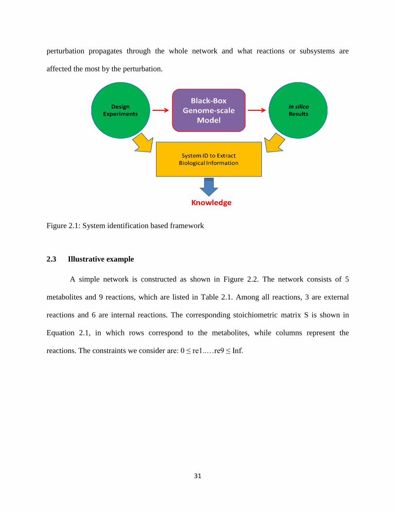
31

perturbation propagates through the whole network and what reactions or subsystems are

affected the most by the perturbation.

Figure 2.1: System identification based framework

2.3 Illustrative example

A simple network is constructed as shown in Figure 2.2. The network consists of 5

metabolites and 9 reactions, which are listed in Table 2.1. Among all reactions, 3 are external

reactions and 6 are internal reactions. The corresponding stoichiometric matrix S is shown in

Equation 2.1, in which rows correspond to the metabolites, while columns represent the

reactions. The constraints we consider are: 0 ≤ re1..…re9 ≤ Inf.

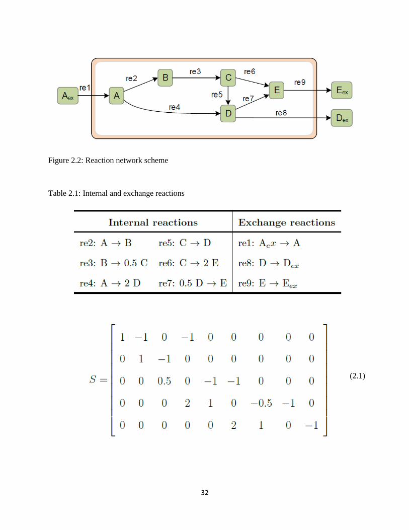
32

Figure 2.2: Reaction network scheme

Table 2.1: Internal and exchange reactions

(2.1)

33

Two case studies have been used here. The first one is to maximize production of metabolite D

as the objective function of FBA, the second one picks maximal production of metabolite E as

the objective function. For both cases, we investigate how the flux distribution would be acted if

we increase the pickup rate of substrate A. In particular, we would like to identify what reactions

are acted most significantly if pickup rate of A increases.

2.3.1 Case study 1: Objective function: maximal flux of re8 (production of D)

In this case study, we first conduct a series of 100 in silico experiments by varying the

flux of re1 (pick up rate of A) from 2 to 4 mmol/gDCW/hr with a step size of 0.02. This set of

experiments results in a 9 x 101 data matrix, with each column represents the 9 reaction fluxes

for a given substrate pick up rate. We then perform PCA on the data matrix, which confirms that

one principal component (PC) captures 100% of the variance contained in the data matrix. The

scaled loading of the PC is plotted in Figure 2.3. With increased substrate pickup rate (which is

scaled to be 1 as the basis), only re4 and re8 are affected with a scale of 1 and 4, which indicates

that flux of re4 increases with the same amount as that of re1while flux of re8 increase 4 times

the amount of increase in flux of re1. It is worth noting that a negative loading in this case would

indicate a decreased ux. Figure 2.4 visualizes the analysis result by highlighting the fluxes that

are affected by increasing flux of re1.

34

Figure 2.3: Scaled PCA loading for case study 1

Figure 2.4: Visualization of the analysis results for case study 1. The reactions that are affected

by increasing flux of re1 are highlighted in blue. The line thickness is proportional to its loading.

2.3.2 Case study 2: Objective function: maximal flux of re9 (production of E)

In this case study, similar steps as in case study 1 were carried out, with the only

difference being in the objective function of FBA. In this case study, the objective function is to

maximize the production of E. The PC loading and network visualization are plotted in Figure

2.5 and Figure 2.6.

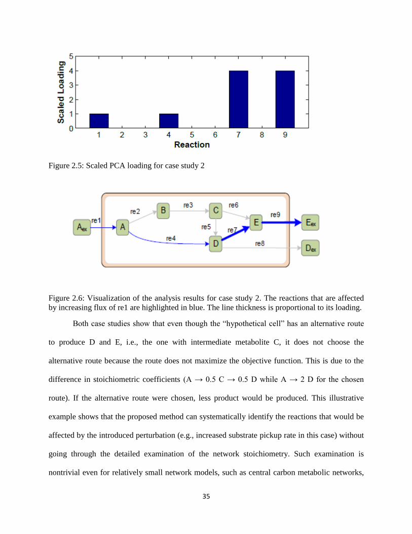
35

Figure 2.5: Scaled PCA loading for case study 2

Figure 2.6: Visualization of the analysis results for case study 2. The reactions that are affected

by increasing flux of re1 are highlighted in blue. The line thickness is proportional to its loading.

Both case studies show that even though the “hypothetical cell” has an alternative route

to produce D and E, i.e., the one with intermediate metabolite C, it does not choose the

alternative route because the route does not maximize the objective function. This is due to the

difference in stoichiometric coefficients (A → 0.5 C → 0.5 D while A → 2 D for the chosen

route). If the alternative route were chosen, less product would be produced. This illustrative

example shows that the proposed method can systematically identify the reactions that would be

affected by the introduced perturbation (e.g., increased substrate pickup rate in this case) without

going through the detailed examination of the network stoichiometry. Such examination is

nontrivial even for relatively small network models, such as central carbon metabolic networks,

36

and quickly becomes infeasible when the size of the network increases. But with the proposed

method, we can easily examine how a perturbation would affect the whole network and identify

the key reactions that are affected the most by the perturbation.

37

Chapter 3: Comprehensive Evaluation of Two GSMMs for S. stipitis

3.1 Introduction

The complete genome of S. stipitis has been sequenced (Jeffries et al., 2007), which

provides the foundation for genome-scale metabolic network reconstruction. Based on the

sequenced genome, several metabolic network models have been published recently (Caspeta et

al., 2012; Balagurunathan et al., 2012; Liu et al., 2012; Liang et al., 2013). Among them, two

genome-scale models: iSS884 (Caspeta et al., 2012) and iBB814 (Balagurunathan et al., 2012)

represent significant steps forward in gaining a systematic understanding of cellular metabolism

of S. stipitis. For metabolic network models, it is clear that the quality of the model determines

the outcome of the application. Therefore, it is critically important to determine how accurate a

metabolic network model is, particularly for a genome-scale model, in describing the

microorganism’s cellular metabolism. Currently model validation is done primarily through wet

lab experiments, i.e., comparing model predictions with experimental measurements. Due to the

cost and technical difficulties associated with getting intracellular measurements, most

experimental measurements are limited to cross membrane fluxes such as substrate uptake rates,

production secretion rates, and cell growth rates. However, due to the scale and complexity

involved in GSMMs, a good agreement between measured and computed cross-membrane fluxes

does not necessarily indicate that the model quality is high. Therefore, new methods are needed

to effectively evaluate the quality of GSMMs. In this work, we propose system identification

(SID) based framework to examine metabolic network models in a systematic way. First, the SID

framework is applied to extract qualitative biological knowledge embedded in GSMMs, which is

difficult, if not impossible, to be obtained through existing methods. Then the extracted

knowledge is compared with the existing knowledge for model quality assessment or validation.

38

3.2 Materials and Methods

The materials that were used were two genome-scale model, iSS884 and iBB814. The

genome-scale metabolic models were evaluated by flux balance analysis (FBA), in which the

COBRA toolbox (Schellenberger et al., 2011) was used. SID framework was used for model

validation. Manual examination of the two genome-scale models was carried out by comparison

of the reaction subsystems.

3.2.1 Two published genome-scale models: iSS884 and iBB814

iSS884 (Caspeta et al., 2012) was constructed semi-automatically by integrating

automatic reconstruction with S. cerevisiae as a reference framework and manual curation and

modification. iBB814 (Balagurunathan et al., 2012) was constructed manually by following a

published protocol (Thiele and Palsson, 2010) for generating a high-quality genome-scale

metabolic reconstruction. iSS884 includes 1332 reactions, 922 metabolites and 4 compartments;

iBB814 includes 1371 reactions, 644 metabolites and 3 compartments. More detailed comparison

can be found in Appendix A1. Both models have significant experimental validations and both

performed well in matching the model predictions with some experimental measurements.

3.2.2 In silico experiments

The genome-scale metabolic models were evaluated by flux balance analysis (FBA), in

which the COBRA toolbox (Schellenberger et al., 2011) was used. For all the simulations, the

objective function was biomass growth. The upper limits of xylose and oxygen uptakes were

varied based on the preselected conditions, while the other exchange compounds (NH4+

, H+,

SO42-

, Pi2-

, H2O, Fe2+

) were given the option to enter and exit the network freely, with upper and

lower bounds of -1000 to 1000 mmol/gDW·hr. The final metabolic products (CO2, ethanol,

acetic acid, etc.) were allowed to exit the system freely, where the reaction flux was constrained

39

to 0 – 1000 mmol/gDW·hr, which prevents product uptake. The growth associated maintenance

energy was set to 2.6 mmol/gDW·hr (Balagurunathan et al., 2012). This setup was applied to all

in silico simulations for both models.

3.2.3 Phenotype phase plane (PhPP) analysis

Phenotype phase plane (PhPP) analysis (Edwards et al., 2002; Bell and Palsson, 2005) is

an extension of FBA that allows the study of metabolic genotype-phenotype relation. Two

substrate parameters are varied independently, such as oxygen and carbon substrate, where the

optimal flux distributions are calculated for all points in the selected plane. There are a finite

number of optimal metabolic flux maps in the plane, which is known as a phenotype phase.

Phenotype phases are each fundamentally distinct based on how model optimally chooses to use

certain pathways. Each phenotype is generated by calculating shadow prices of the metabolites

throughout the plane. Shadow price is a linear programming term used to define the sensitivity of

a parameter on the objective function, and can be calculated from the dual solution in a linear

programming problem. In this case, the parameter is the metabolite, and the objective function is

the growth rate. Therefore in each phenotype, each metabolite will have a constant value, and are

different in other phenotypes. Phenotype phase plane (PhPP) analysis was performed on iSS884

and iBB814 in order to gain a global view on the growth and the production of ethanol and CO2,

with xylose and oxygen as the two independent variables. The phenotypes were specified by

color.

3.2.4 Conventional point-matching using experimental data

We also carried out experimental validations in a traditional way, which consists of both

quantitative and qualitative validations. For quantitative validation, the substrate (xylose,

glucose, and oxygen) uptake rates were set to be the same as the experimentally operated value,

40

then the model predictions of the production secretion rates (CO2, ethanol, cell growth) were

compared with the experimental reported values to assess the model accuracy. For qualitative

validation, the validation experiments for inhibition and mutants were implemented by removing

relevant reactions from the network models, and then the predictions of the modified models

were compared with reported experimental outcomes, where the results were evaluated by

checking if there was cell growth or product secretion.

3.2.5 System identification (SID) framework

As already discussed, SID framework was used to take heavily computation quantitative

results that come from prepared in silico experiments, and extracted embedded biological

knowledge through PCA. The results are then visualized through metabolic colored maps. Being

qualitative in nature, this allows for biologist to easily interpret this information and make

system guided decisions.

3.2.6 Manual Examination

The published models were written in different metabolites labeling schemes, so the first

step was to convert iSS884 metabolites to the naming formulation of iBB814. Different reactions

were categorized by subsystems and pathways, where the reactions of the two models were

compared by subsystems/pathways to assess their similarities and differences. The KEGG

database was used to obtain strain specific information on different reactions. Finally, the

components and stoichiometry of the biomass growth equation were compared.

3.3 Results and Discussion

As discussed earlier, the two published models represent significant steps forward

towards a better systems level understanding of S. stipitis’ metabolism. At the same time, despite

41

the fact that both models have significant experimental validations and both performed well in

matching the model predictions with some experimental measurements, they have limitations.

This is expected since they were the first genome-scale models on S. stipitis. For example,

neither model predicts the production of xylitol under any condition – aerobic, oxygen-limited or

anaerobic. It is well-known that xylitol is a key byproduct produced by S. stipitis under oxygen-

limited condition due the redox imbalance caused by xylose fermentation step (XR and XDH)

(Slininger et al., 1985; Slininger et al., 1991). Therefore, being able to predict xylitol production

under oxygen limitation is very important – especially if the model to help identify candidates

for balancing cellular redox potential, as well as for mutant development.

In this work, comprehensive evaluations of the two genome-scale models (iSS884 and

iBB814) were conducted with the aim to detect potential errors and to identify a model that

agrees better with existing biological knowledge to serve as the basis for further model

improvement. To achieve this goal, we first conducted various in silico experiments to examine

each model’s global behavior through phenotype phase plane (PhPP) analysis, and to compare

the model predictions with additional experimental results reported in literature. However, the

obtained results from this step led to conflicting conclusions. Next, we designed in silico

experiments and applied the proposed system identification framework to extract biological

knowledge from the in silico experimental data. We then examined whether the extracted

knowledge agrees with existing understandings. The system identification approach identified

several key abnormal behaviors in both models, and detailed analyses show that in general

iBB814 agrees with existing understanding better. Finally, to pinpoint the fundamental reasons

(i.e., which reactions in the network) for the abnormal behaviors, we conducted thorough manual

examination of the models. Guided by the results obtained from the system identification

42

approach, the major artifacts of both models were identified, which provides some explanations

for the abnormal behaviors of both models.

3.3.1 Model comparison using the existing methods

In this section, the following existing methods were carried out to compare the two

models: PhPP analysis and conventional point-matching using experimental data. Simulations

were conducted in MATLAB using COBRA toolbox (Schellenberger et al., 2011) to carry out

FBA in calculating the fluxes of different reactions, which in the literature is known as in silico

experiments.

3.3.1.1 Phenotype phase plane (PhPP) analysis

In this analysis, xylose and oxygen uptake rates were chosen as the independent

variables, with each of them varying from 0 – 10 mmol/gDW·hr. Figure 3.1 (a) and (b) show

how cell growth rate is affected by different substrate uptake rates, where the differently colored

regions represent different growth behaviors. Overall, cell growth profiles predicted by iSS884

and iBB814 are similar to each other, except that the growth rate predicted by iBB814 is

significantly lower than iSS884. The ethanol and CO2 production profiles predicted by the two

models are shown in Figure 3.1 (c) and (e) for iSS884, (d) and (f) for iBB814. The ethanol

profiles are similar between the models, except that iSS884 predicts a larger area of zero ethanol

production, which is shown as the green phenotype. The CO2 profiles are similar between the

two models as well. Overall, Figure 3.1 indicates that both models have their share of similarities

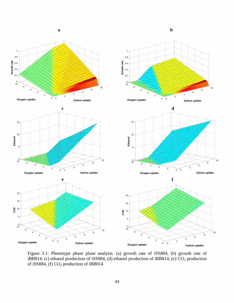
43

f

Figure 3.1: Phenotype phase plane analysis. (a) growth rate of iSS884, (b) growth rate of

iBB814, (c) ethanol production of iSS884, (d) ethanol production of iBB814, (e) CO2 production

of iSS884, (f) CO2 production of iBB814

a b

c d

e

02

46

810

0

2

4

6

8

100

0.2

0.4

0.6

0.8

1

Xylose uptake Oxygen uptake

Gro

wth

ra

te

02

46

810

0

2

4

6

8

100

0.2

0.4

0.6

0.8

1

Xylose uptake Oxygen uptake

Gro

wth

ra

te

2

46

8

10

02

46

8100

5

10

15

Xylose uptakeOxygen uptake

Eth

an

ol

24

68

10

02

46

8100

5

10

15

Xylose uptakeOxygen uptake

Eth

an

ol

02

46

810

0

2

4

6

8

100

5

10

15

20

Xylose uptake Oxygen uptake

CO

2

02

46

810

0

2

4

6

8

100

5

10

15

20

Xylose uptake Oxygen uptake

CO

2

44

and differences. It is difficult to conclude which model is better, as the differences are subtle and

no complete set of experimental data is available that covers the ranges of oxygen and xylose

uptake rates for model validation and comparison.

3.3.1.2 Conventional point-matching using experimental data

To further compare the models, we use several experimental data sets reported in the

literature to carry out model validation in a traditional way. To provide a fair comparison, model

validation consists of two quantitative and two qualitative case studies. One quantitative data set

was from (Caspeta et al., 2012), in which iSS884 model was published; the other was from an

independent source (Li, 2012). In addition, one qualitative data set was from (Balagurunathan et

al., 2012), in which iBB814 model was published, the other was from an independent source (Jin

et al., 2005).

For quantitative validation, Figure 3.2 shows the comparison results using the

experimental data reported in (Caspeta et al., 2012). The model inputs (i.e., xylose and oxygen)

were set to the experimental values, and model predictions (i.e., biomass, ethanol and CO2

fluxes) were compared with the experimental values at three different oxygen utilization rates

(OUR). From Figure 3.2, it appears that iSS884 performs better than iBB814, particularly for

the biomass growth.

Figure 3.3 shows the comparison results using the independent data set reported in (Li,

2012). This case study consists of four experimental conditions: two carbon sources (glucose and

xylose) combined with two oxygenation conditions (aerobic and oxygen-limited). Similar to the

previous case study, the model inputs (i.e., xylose or glucose, and oxygen) were set to the

experimental values, and model predictions (i.e., ethanol, CO2, and biomass) were compared

with experimental values.

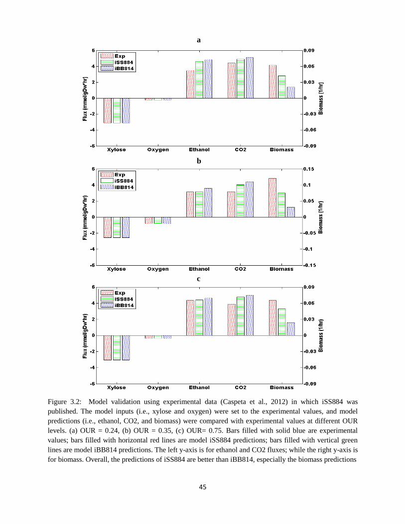
45

Figure 3.2: Model validation using experimental data (Caspeta et al., 2012) in which iSS884 was

published. The model inputs (i.e., xylose and oxygen) were set to the experimental values, and model

predictions (i.e., ethanol, CO2, and biomass) were compared with experimental values at different OUR

levels. (a) OUR = 0.24, (b) OUR = 0.35, (c) OUR= 0.75. Bars filled with solid blue are experimental

values; bars filled with horizontal red lines are model iSS884 predictions; bars filled with vertical green

lines are model iBB814 predictions. The left y-axis is for ethanol and CO2 fluxes; while the right y-axis is

for biomass. Overall, the predictions of iSS884 are better than iBB814, especially the biomass predictions

a

a

b

c

a

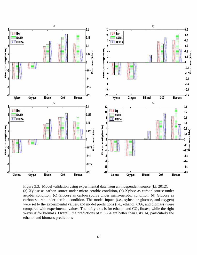
46

Figure 3.3: Model validation using experimental data from an independent source (Li, 2012).

(a) Xylose as carbon source under micro-aerobic condition, (b) Xylose as carbon source under

aerobic condition, (c) Glucose as carbon source under micro-aerobic condition, (d) Glucose as

carbon source under aerobic condition. The model inputs (i.e., xylose or glucose, and oxygen)

were set to the experimental values, and model predictions (i.e., ethanol, CO2, and biomass) were

compared with experimental values. The left y-axis is for ethanol and CO2 fluxes; while the right

y-axis is for biomass. Overall, the predictions of iSS884 are better than iBB814, particularly the

ethanol and biomass predictions

a b

c d

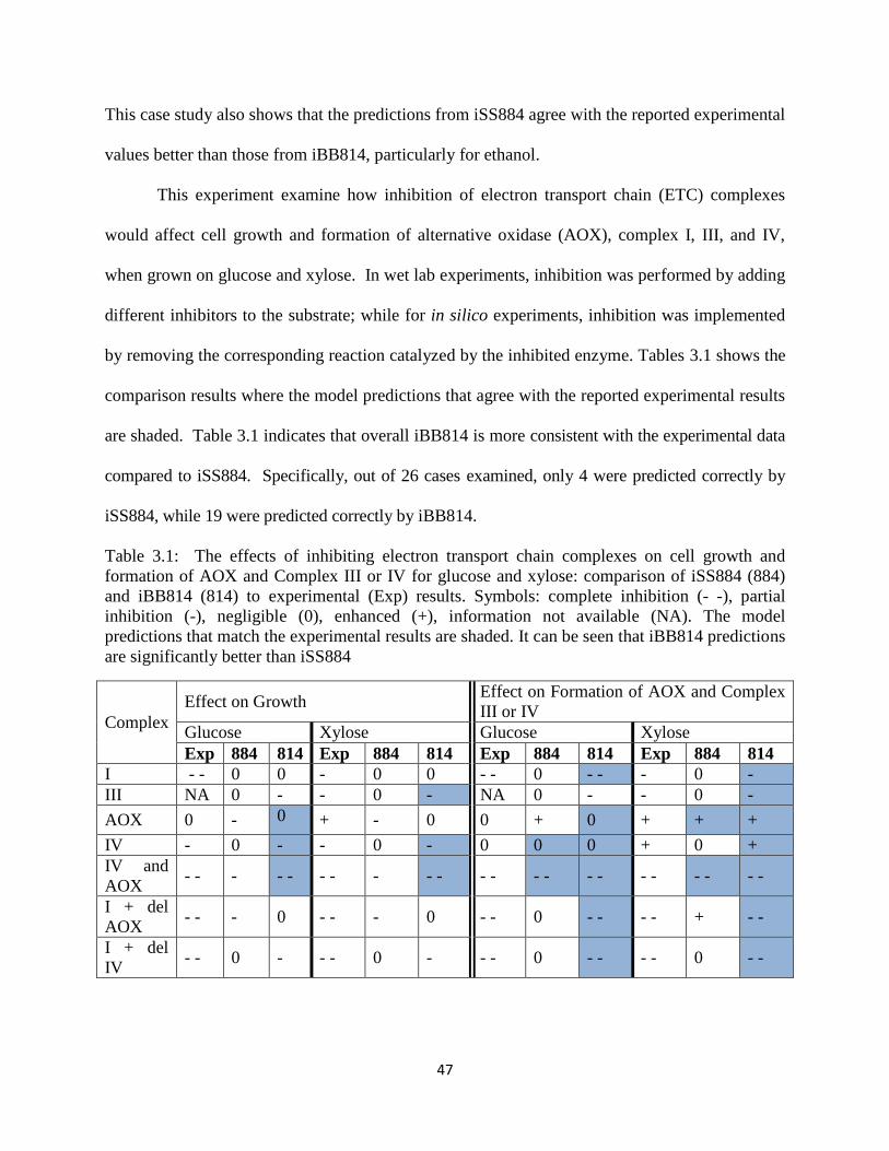
47

This case study also shows that the predictions from iSS884 agree with the reported experimental

values better than those from iBB814, particularly for ethanol.

This experiment examine how inhibition of electron transport chain (ETC) complexes

would affect cell growth and formation of alternative oxidase (AOX), complex I, III, and IV,

when grown on glucose and xylose. In wet lab experiments, inhibition was performed by adding

different inhibitors to the substrate; while for in silico experiments, inhibition was implemented

by removing the corresponding reaction catalyzed by the inhibited enzyme. Tables 3.1 shows the

comparison results where the model predictions that agree with the reported experimental results

are shaded. Table 3.1 indicates that overall iBB814 is more consistent with the experimental data

compared to iSS884. Specifically, out of 26 cases examined, only 4 were predicted correctly by

iSS884, while 19 were predicted correctly by iBB814.

Table 3.1: The effects of inhibiting electron transport chain complexes on cell growth and

formation of AOX and Complex III or IV for glucose and xylose: comparison of iSS884 (884)

and iBB814 (814) to experimental (Exp) results. Symbols: complete inhibition (- -), partial

inhibition (-), negligible (0), enhanced (+), information not available (NA). The model

predictions that match the experimental results are shaded. It can be seen that iBB814 predictions

are significantly better than iSS884

Complex

Effect on Growth Effect on Formation of AOX and Complex

III or IV

Glucose Xylose Glucose Xylose

Exp 884 814 Exp 884 814 Exp 884 814 Exp 884 814

I - - 0 0 - 0 0 - - 0 - - - 0 -

III NA 0 - - 0 - NA 0 - - 0 -

AOX 0 - 0 + - 0 0 + 0 + + +

IV - 0 - - 0 - 0 0 0 + 0 +

IV and

AOX - - - - - - - - - - - - - - - - - - - - - -

I + del

AOX - - - 0 - - - 0 - - 0 - - - - + - -

I + del

IV - - 0 - - - 0 - - - 0 - - - - 0 - -

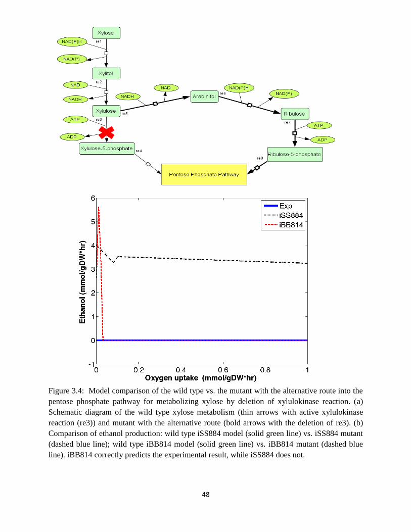
48

Figure 3.4: Model comparison of the wild type vs. the mutant with the alternative route into the

pentose phosphate pathway for metabolizing xylose by deletion of xylulokinase reaction. (a)

Schematic diagram of the wild type xylose metabolism (thin arrows with active xylulokinase

reaction (re3)) and mutant with the alternative route (bold arrows with the deletion of re3). (b)

Comparison of ethanol production: wild type iSS884 model (solid green line) vs. iSS884 mutant

(dashed blue line); wild type iBB814 model (solid green line) vs. iBB814 mutant (dashed blue

line). iBB814 correctly predicts the experimental result, while iSS884 does not.

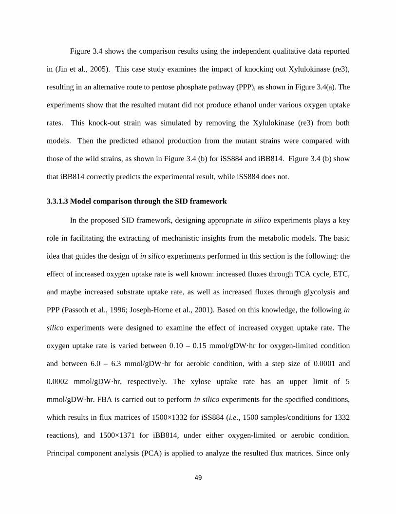
49

Figure 3.4 shows the comparison results using the independent qualitative data reported

in (Jin et al., 2005). This case study examines the impact of knocking out Xylulokinase (re3),

resulting in an alternative route to pentose phosphate pathway (PPP), as shown in Figure 3.4(a). The

experiments show that the resulted mutant did not produce ethanol under various oxygen uptake

rates. This knock-out strain was simulated by removing the Xylulokinase (re3) from both

models. Then the predicted ethanol production from the mutant strains were compared with

those of the wild strains, as shown in Figure 3.4 (b) for iSS884 and iBB814. Figure 3.4 (b) show

that iBB814 correctly predicts the experimental result, while iSS884 does not.

3.3.1.3 Model comparison through the SID framework

In the proposed SID framework, designing appropriate in silico experiments plays a key

role in facilitating the extracting of mechanistic insights from the metabolic models. The basic

idea that guides the design of in silico experiments performed in this section is the following: the

effect of increased oxygen uptake rate is well known: increased fluxes through TCA cycle, ETC,

and maybe increased substrate uptake rate, as well as increased fluxes through glycolysis and

PPP (Passoth et al., 1996; Joseph-Horne et al., 2001). Based on this knowledge, the following in

silico experiments were designed to examine the effect of increased oxygen uptake rate. The

oxygen uptake rate is varied between 0.10 – 0.15 mmol/gDW·hr for oxygen-limited condition

and between 6.0 – 6.3 mmol/gDW·hr for aerobic condition, with a step size of 0.0001 and

0.0002 mmol/gDW·hr, respectively. The xylose uptake rate has an upper limit of 5

mmol/gDW·hr. FBA is carried out to perform in silico experiments for the specified conditions,

which results in flux matrices of 1500×1332 for iSS884 (i.e., 1500 samples/conditions for 1332

reactions), and 1500×1371 for iBB814, under either oxygen-limited or aerobic condition.

Principal component analysis (PCA) is applied to analyze the resulted flux matrices. Since only

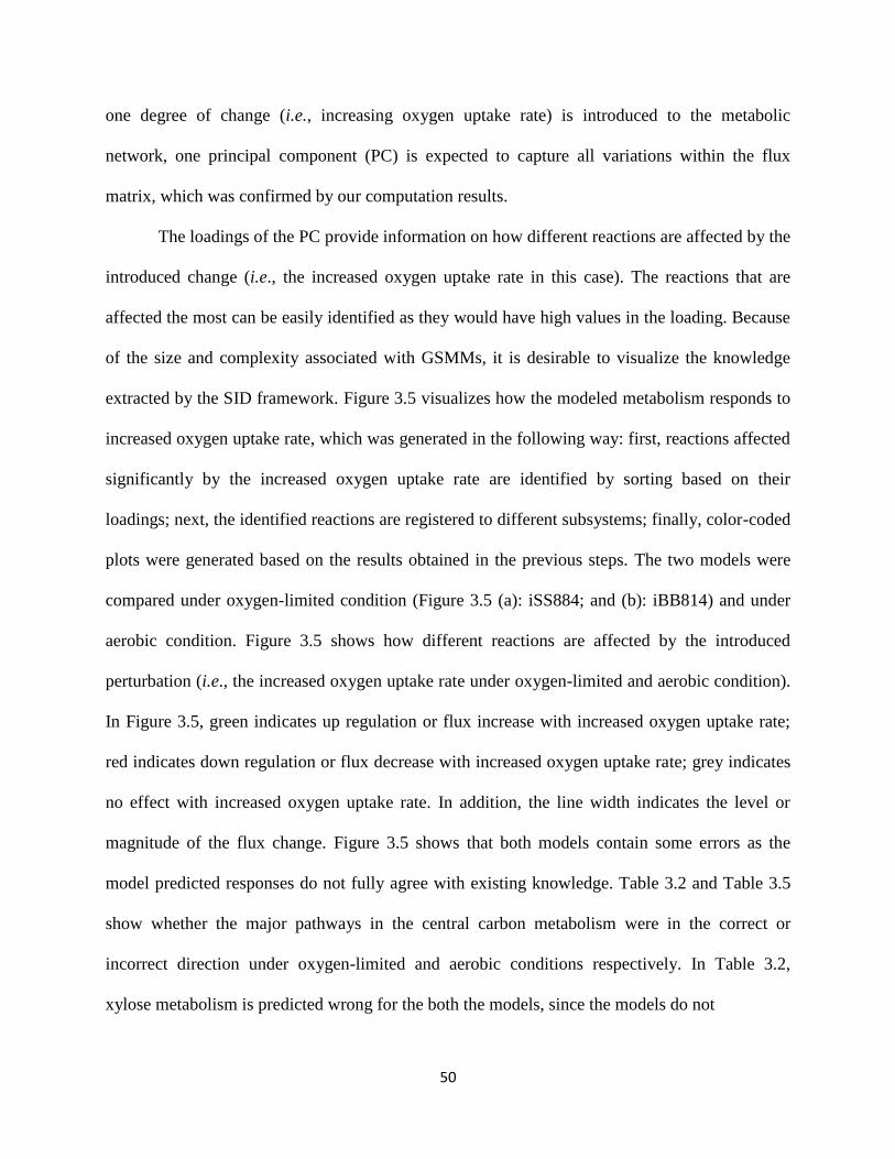
50

one degree of change (i.e., increasing oxygen uptake rate) is introduced to the metabolic

network, one principal component (PC) is expected to capture all variations within the flux

matrix, which was confirmed by our computation results.

The loadings of the PC provide information on how different reactions are affected by the

introduced change (i.e., the increased oxygen uptake rate in this case). The reactions that are

affected the most can be easily identified as they would have high values in the loading. Because

of the size and complexity associated with GSMMs, it is desirable to visualize the knowledge

extracted by the SID framework. Figure 3.5 visualizes how the modeled metabolism responds to

increased oxygen uptake rate, which was generated in the following way: first, reactions affected

significantly by the increased oxygen uptake rate are identified by sorting based on their

loadings; next, the identified reactions are registered to different subsystems; finally, color-coded

plots were generated based on the results obtained in the previous steps. The two models were

compared under oxygen-limited condition (Figure 3.5 (a): iSS884; and (b): iBB814) and under

aerobic condition. Figure 3.5 shows how different reactions are affected by the introduced

perturbation (i.e., the increased oxygen uptake rate under oxygen-limited and aerobic condition).

In Figure 3.5, green indicates up regulation or flux increase with increased oxygen uptake rate;

red indicates down regulation or flux decrease with increased oxygen uptake rate; grey indicates

no effect with increased oxygen uptake rate. In addition, the line width indicates the level or

magnitude of the flux change. Figure 3.5 shows that both models contain some errors as the

model predicted responses do not fully agree with existing knowledge. Table 3.2 and Table 3.5

show whether the major pathways in the central carbon metabolism were in the correct or

incorrect direction under oxygen-limited and aerobic conditions respectively. In Table 3.2,

xylose metabolism is predicted wrong for the both the models, since the models do not

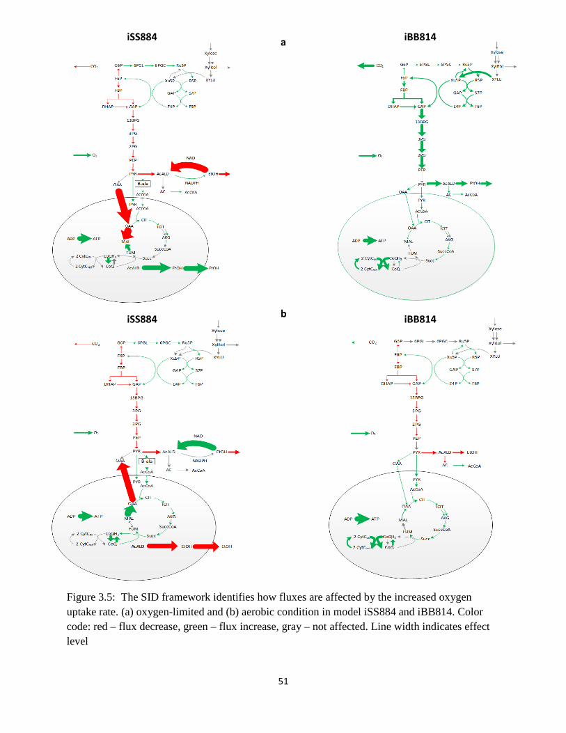
51

Figure 3.5: The SID framework identifies how fluxes are affected by the increased oxygen

uptake rate. (a) oxygen-limited and (b) aerobic condition in model iSS884 and iBB814. Color

code: red – flux decrease, green – flux increase, gray – not affected. Line width indicates effect

level

iSS884 iBB814 b

iSS884 iBB814 a

52

predict xylitol production. Both branches of the PPP are correct in iSS884, while iBB814 behave

in the opposite response. Glycolysis is the only pathway that was correct for both models. The

TCA cycle was expected to be branched for oxygen-limited condition, which was the case for

iSS884, and the ETC was in the correct direction for iBB814. The errors from the branches of

PPP in iBB814 could be contributed to the lack of xylitol production. Looking at the TCA cycle,

we see that the advent of acetyl-CoA into the mitochondria occurs by different routes, which

seems unusual since the pathways of the central carbon metabolism have been firmly established.

In iSS884, pyruvate does not enter TCA cycle directly under either oxygen-limited or aerobic

condition, while in iBB814 it does..

Table 3.2: SID results of iSS884 and iBB814 under oxygen-limited condition. The symbol

represents the correct direction from the model and represents the incorrect direction from

the model.

Pathways iSS884 iBB814

Xylose metabolism

Oxidative - PPP

Non-oxidative – PPP

Glycolysis

TCA cycle

ETC

In iSS884, pyruvate enters amino acid metabolism, as well as being used for ethanol production,

without being converted into acetyl-CoA. Further investigation was done using the SID

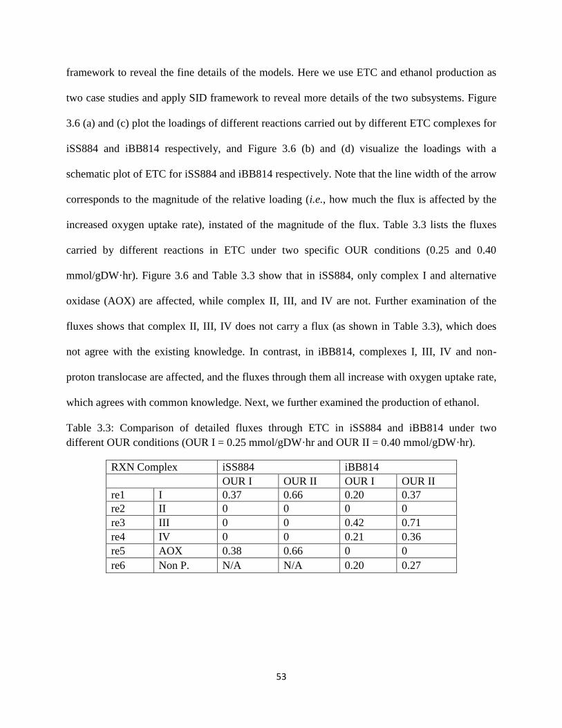
53

framework to reveal the fine details of the models. Here we use ETC and ethanol production as

two case studies and apply SID framework to reveal more details of the two subsystems. Figure

3.6 (a) and (c) plot the loadings of different reactions carried out by different ETC complexes for

iSS884 and iBB814 respectively, and Figure 3.6 (b) and (d) visualize the loadings with a

schematic plot of ETC for iSS884 and iBB814 respectively. Note that the line width of the arrow

corresponds to the magnitude of the relative loading (i.e., how much the flux is affected by the

increased oxygen uptake rate), instated of the magnitude of the flux. Table 3.3 lists the fluxes

carried by different reactions in ETC under two specific OUR conditions (0.25 and 0.40

mmol/gDW·hr). Figure 3.6 and Table 3.3 show that in iSS884, only complex I and alternative

oxidase (AOX) are affected, while complex II, III, and IV are not. Further examination of the

fluxes shows that complex II, III, IV does not carry a flux (as shown in Table 3.3), which does

not agree with the existing knowledge. In contrast, in iBB814, complexes I, III, IV and non-

proton translocase are affected, and the fluxes through them all increase with oxygen uptake rate,

which agrees with common knowledge. Next, we further examined the production of ethanol.

Table 3.3: Comparison of detailed fluxes through ETC in iSS884 and iBB814 under two

different OUR conditions (OUR I = 0.25 mmol/gDW·hr and OUR II = 0.40 mmol/gDW·hr).

RXN Complex iSS884 iBB814

OUR I OUR II OUR I OUR II

re1 I 0.37 0.66 0.20 0.37

re2 II 0 0 0 0

re3 III 0 0 0.42 0.71

re4 IV 0 0 0.21 0.36

re5 AOX 0.38 0.66 0 0

re6 Non P. N/A N/A 0.20 0.27

54

Figure 3.6: Comparison of electron transport chain (ETC) through the SID framework for iSS884

and iBB814 under oxygen-limited condition: (a) Relative loading plots for iSS884 and (c)

iBB814. (b) Schematic diagram of the machinery in the ETC for iSS884 and (d) iBB814, where

the line weight corresponds to the magnitude of the relative loading for the different machinery

shown in (a) and (c).

Table 3.4 shows the fluxes carried by different reactions in iSS884 and iBB814 under

OUR = 0.10. From Table 3.4, we see that in iSS884 the major production of ethanol occurs in

the mitochondria, while the cytosol reaction converts NADH to NADPH, with both fluxes

I II III IV AOX Non P.0

0.5

1

1.5

2

2.5

3

Reactions

Re

lati

ve

Lo

ad

ing

I II III IV AOX Non P.0

0.5

1

1.5

2

2.5

3

Reactions

Re

lati

ve

Lo

ad

ing

a b

c d

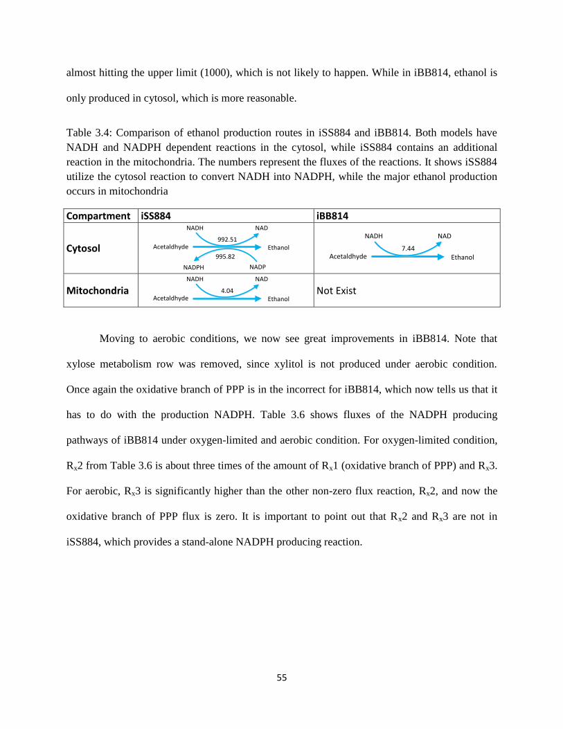
55

almost hitting the upper limit (1000), which is not likely to happen. While in iBB814, ethanol is

only produced in cytosol, which is more reasonable.

Table 3.4: Comparison of ethanol production routes in iSS884 and iBB814. Both models have

NADH and NADPH dependent reactions in the cytosol, while iSS884 contains an additional

reaction in the mitochondria. The numbers represent the fluxes of the reactions. It shows iSS884

utilize the cytosol reaction to convert NADH into NADPH, while the major ethanol production

occurs in mitochondria

Compartment iSS884 iBB814

Cytosol Acetaldhyde Ethanol

NADH NAD

NADPH NADP

995.82

992.51

Acetaldhyde Ethanol

NADH NAD

7.44

Mitochondria Acetaldhyde Ethanol

NADH NAD

4.04

Not Exist

Moving to aerobic conditions, we now see great improvements in iBB814. Note that

xylose metabolism row was removed, since xylitol is not produced under aerobic condition.

Once again the oxidative branch of PPP is in the incorrect for iBB814, which now tells us that it

has to do with the production NADPH. Table 3.6 shows fluxes of the NADPH producing

pathways of iBB814 under oxygen-limited and aerobic condition. For oxygen-limited condition,

Rx2 from Table 3.6 is about three times of the amount of Rx1 (oxidative branch of PPP) and Rx3.

For aerobic, Rx3 is significantly higher than the other non-zero flux reaction, Rx2, and now the

oxidative branch of PPP flux is zero. It is important to point out that Rx2 and Rx3 are not in

iSS884, which provides a stand-alone NADPH producing reaction.

56

Table 3.5: SID results of iSS884 and iBB814 aerobic condition. The symbol represents the

correct direction from the model and represents the incorrect direction from the model

Pathways iSS884 iBB814

Oxidative - PPP

Non-oxidative – PPP

Glycolysis

TCA cycle

ETC

Table 3.6: NADPH production pathways for iBB814. Oxygen-limited condition: OUR I = 0.20

mmol/gDW·hr and OUR II = 0.35 mmol/gDW·hr. Aerobic condition: OUR I = 6.0

mmol/gDW·hr and OUR II = 6.3 mmol/gDW·hr. 6pgc: 6-phosphogluconate, ru5p-D: ribulose 5-

phosphate, acald: acetaldehyde, ac: acetic acid, icit: isocitrate, akg: alpha-ketoglutarate

Rx Reaction Oxygen-limited Aerobic

OUR I OUR II OUR I OUR II

1 nadp[c]+ 6pgc[c] -> nadph[c] + co2[c] + ru5p-D[c]

0.026 0.023 0 0

2 h2o[c] + nadp[c] + acald[c] -> 2 h[c] + nadph[c] +

ac[c]

0.092 0.085 0.038 0.031

3 nadp[c] + icit[c] -> akg[c] + nadph[c] + co2[c] 0.030 0.034 0.59 0.62

57

3.3.1.4 Manual examination guided by the SID framework

In Section 3.3.1.3, several system level differences between the two models have been

revealed by the SID framework. To confirm these findings and to identify the root causes (e.g.,

specific reactions) that result in the different model behaviors, manual examination was carried

out to compare the reactions, metabolites, genes and compartments. Figure 3.7 (a) shows the

number of reactions in different subsystems that are unique to or overlap between iSS884 and

iBB814. Overall, the two models often share less than one-half to one-third of the reactions, with

the least overlap in the lipid subsystem. Specifically, one major difference in the lipid subsystem

is the formulation procedure of saturated fatty acid: iSS884 uses a stepwise procedure, which has

more intermediate steps, while iBB814 is simplified. The details on saturated fatty acid

biosynthesis can be found in Appendix A2. In summary, iBB814 provides more flexibility, since

a fatty acid of any even length between 2 and 26 can be formed. In contrast, iSS884 employs a

linear stepwise reaction which only produces the fatty acid with 12, 14, 16 and 18 carbons, while

the shorter chain fatty acids are only used as the intermediates because they are all ACP bonded.

The amount of amino reactions in both models is about the same and between the models

they more than half of the reactions. The amino acid subsystems are crucial to the metabolism,

since they represent a majority of the metabolites in the biomass reaction. Analysis was done on

the amino acid subsystems to see what routes the models took for amino acid production. Table

3.7 shows the results of the amino acids for the models, where 11 out of the 19 amino acid

reactions were the same. For the ones that were different, 3 dealt with different cofactors usage

(L-glutamate, L-histidine, and L-proline). In L-alanine the reaction was the same, but iSS884

occurred in the cytosol and iBB814 in the mitochondria. The other 4 amino acids (L-cysteine,

glycine, L-serine, and L-valine) were from different precursors.

58

Figure 3.7: Comparison of constituent reactions in iSS884 and iBB814: (a) subsystem

breakdown, (b) central carbon metabolism breakdown. AA – amino acids, Nuc – nucleotides,

Carbs – carbohydrates, CCM- central carbon metabolism, CV- cofactors and vitamins, TCA –

tricarboxylic acid cycle, Glyc – Glycolysis, PPP – pentose phosphate pathway, ETC – electron

transport chain, XM- xylose metabolism, PM – pyruvate metabolism. Legend: Bars filled with

horizontal red lines – number of reactions unique to iSS884; Bars filled with vertical green lines

are number of reactions unique to iBB814; Bars filled with solid blue are number of reactions

shared between iSS884 and iBB814

0

50

100

150

200

250

300

AA Lipids Nuc Carbs CCM CV

Nu

mb

er o

f R

eact

ion

s Unique to iSS884

Unique to iBB814

Shared

0

5

10

15

20

25

30

35

40

TCA Glyc PPP ETC XM PM

Nu

mb

er o

f R

eact

ion

s

Unique to iSS884

Unique to iBB814

Shared

59

Table 3.7: Amino acid production routes under oxygen-limited condition

Amino Acids iSS884 iBB814 Description

L-Alanine [c] [m] Same reaction

L-Arginine Same reaction

L-Asparagine same reaction

L-Aspartate Same reaction

L-Cysteine serine acetyl-serine Both use hydrogen sulfide

L-Glutamine Same reaction

L-Glutamate nadph nadh Same reaction different

redox

Glycine 2 rxns used Different reaction

L-Histidine nad 2 nad Same reaction - different

redox amounts

L-Isoleucine Same reaction

L-Leucine Same reaction

L-Lysine Same reaction

L-

Phenylalanine

Same reaction

L-Proline nadh nadph Same reaction - different

redox

L-Serine [m] gly [c] rxn fpser Different reaction

L-Threonine Same reaction

L-Tryptophan Same reaction

L-Tyrosine Same reaction

L-Valine[c] from ala-L from glu-L Different reaction

Despite the models have a lot of different amino acid reactions, when looking at the

reactions that are activated they are quite similar. It was surprising to see the central carbon

metabolism (CCM) show a lot of differences, because these pathways have been well studied.

Figure 3.7 (b) shows the number of reactions of different pathways in the CCM that is

unique or overlaps between iSS884 and iBB814. Again the two models share less than one-half

of the reactions in any of the pathways. For the TCA cycle, the main finding is that iSS884

contains more detailed reactions, i.e. more intermediates are included. These metabolites were

linked with the pyruvate metabolism, which is another subsystem that shows a lot of

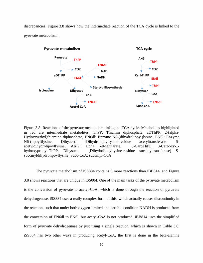
60

discrepancies. Figure 3.8 shows how the intermediate reaction of the TCA cycle is linked to the

pyruvate metabolism.

PyruvateThPP

aDThPP

CO2

Isoleucine

EN6l

Dihyacet

Acetyl-CoA

Steroid Biosynthesis

AKG

CarbThPP

Succ-CoA

Dihysucc

ThPP

CO2

EN6l

ThPP

EN6dl

EN6dl

CoA

EN6dl

CoA

NADH

NAD

Pyruvate metabolism TCA cycle

Figure 3.8: Reactions of the pyruvate metabolism linkage to TCA cycle. Metabolites highlighted

in red are intermediate metabolites. ThPP: Thiamin diphosphate, aDThPP: 2-(alpha-

Hydroxyethyl)thiamine diphosphate, EN6dl: Enzyme N6-(dihydrolipoyl)lysine, EN6l: Enzyme

N6-(lipoyl)lysine, Dihyacet: [Dihydrolipoyllysine-residue acetyltransferase] S-

acetyldihydrolipoyllysine, AKG: alpha ketoglutarate, 3-CarbThPP: 3-Carboxy-1-

hydroxypropyl-ThPP, Dihysucc: [Dihydrolipoyllysine-residue succinyltransferase] S-

succinyldihydrolipoyllysine, Succ-CoA: succinyl-CoA

The pyruvate metabolism of iSS884 contains 8 more reactions than iBB814, and Figure

3.8 shows reactions that are unique in iSS884. One of the main tasks of the pyruvate metabolism

is the conversion of pyruvate to acetyl-CoA, which is done through the reaction of pyruvate

dehydrogenase. iSS884 uses a really complex form of this, which actually causes discontinuity in

the reaction, such that under both oxygen-limited and aerobic condition NADH is produced from

the conversion of EN6dl to EN6l, but acetyl-CoA is not produced. iBB814 uses the simplified

form of pyruvate dehydrogenase by just using a single reaction, which is shown in Table 3.8.

iSS884 has two other ways in producing acetyl-CoA, the first is done in the beta-alanine

61

pathway, which begins at the precursor, L-aspartate, and three reactions follow for production of

acetyl-CoA. The acetyl-CoA that is produced from the beta-alanine pathway occurs in the

cytosol, where it is then converted into another metabolite which is then transported into the

mitochondria and later reconverted to acetyl-CoA. Based on fundamental biochemistry

knowledge and thermodynamics, this passage seems quite unrealistic. A final point to talk about

on the pyruvate metabolism of iSS884 is the absence of aldehyde dehydgronase, which is an

essential reaction for the production of NADPH, we have seen in the last section in Table 3.6

that it carries the highest flux for the production of NADPH for iBB814.

Moving to the TCA cycle, in the mitochondria, iBB8814 can utilize both NAD+ and

NADP+ for isocitrate dehydrogenase, while iSS884 only utilizes NAD+. In cytosol, iBB814 uses

NADP+ while iSS884 uses NAD+, where these reactions can be seen in Table 3.8. Under both

oxygen-limited and aerobic condition, iBB814 utilizes all isocitrate dehydrogenase reactions.

Other major metabolic differences between the two models are summarized in Table 3.8,

where the key metabolic artifacts are listed. It is somewhat surprising to see that iSS884 does not

include NADH-coupled xylose reductase activity, which should be considered greatly important

when considering the redox balance during xylose assimilation. iBB814 uses solely the NADH-

coupled xylose reductase reaction. By combining with the findings obtained from Section

3.3.1.3, we believe that the differences in the cofactor utilization in the central carbon

metabolism as cited above are some of the fundamental reasons for the different behaviors of the

two models, due to the role that redox balancing plays in xylose fermentation.

For ETC, the number of protons being transported from the mitochondrial to the cytosol

in Complex I, III, and IV are different between the two models. Generally speaking, more

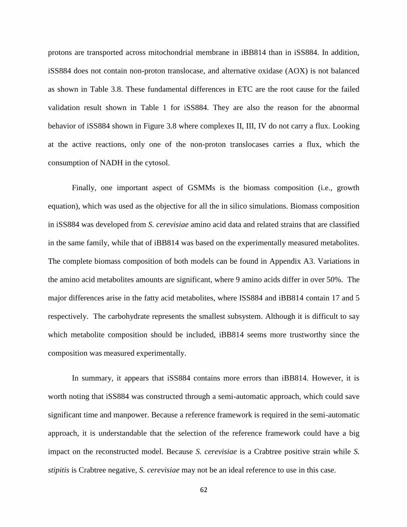
62

protons are transported across mitochondrial membrane in iBB814 than in iSS884. In addition,

iSS884 does not contain non-proton translocase, and alternative oxidase (AOX) is not balanced

as shown in Table 3.8. These fundamental differences in ETC are the root cause for the failed

validation result shown in Table 1 for iSS884. They are also the reason for the abnormal

behavior of iSS884 shown in Figure 3.8 where complexes II, III, IV do not carry a flux. Looking

at the active reactions, only one of the non-proton translocases carries a flux, which the

consumption of NADH in the cytosol.

Finally, one important aspect of GSMMs is the biomass composition (i.e., growth

equation), which was used as the objective for all the in silico simulations. Biomass composition

in iSS884 was developed from S. cerevisiae amino acid data and related strains that are classified

in the same family, while that of iBB814 was based on the experimentally measured metabolites.

The complete biomass composition of both models can be found in Appendix A3. Variations in

the amino acid metabolites amounts are significant, where 9 amino acids differ in over 50%. The

major differences arise in the fatty acid metabolites, where ISS884 and iBB814 contain 17 and 5

respectively. The carbohydrate represents the smallest subsystem. Although it is difficult to say

which metabolite composition should be included, iBB814 seems more trustworthy since the

composition was measured experimentally.

In summary, it appears that iSS884 contains more errors than iBB814. However, it is

worth noting that iSS884 was constructed through a semi-automatic approach, which could save

significant time and manpower. Because a reference framework is required in the semi-automatic

approach, it is understandable that the selection of the reference framework could have a big

impact on the reconstructed model. Because S. cerevisiae is a Crabtree positive strain while S.

stipitis is Crabtree negative, S. cerevisiae may not be an ideal reference to use in this case.

63

Table 3.8: Metabolic artifacts that differ between iSS884 and iBB814

Reaction iSS884 iBB814

Xylose reductase:

NADH Absent H[c] + NADH[c] + XYL-D[c]

NAD[c] + XYLT[c]

Pyruvate

Dehydrogense Complex Form Fig. 3.8

CoA[m] + NAD[m] + PYR[m]

ACCoA[m] + CO2[m] + NADH[m]

Isocitrate

Dehydrogenase

ICIT[m] + NAD[m] AKG[m] +

CO2[m] + NADH[m]

ICIT[m] + NAD[m] AKG[m] +

CO2[m] + NADH[m]

ICIT[m] + NADP[m] AKG[m] +

CO2[m] + NADPH[m]

ICIT[c] + NAD[c] AKG[c] + CO2[c]

+ NADH[c]

ICIT[c] + NADP[c] AKG[c] +

CO2[c] + NADPH[c]

Aldehyde

Dehydgronase NADP

dependent

Absent ACALD[c] + NADP[c] + H2O[c]

NADPH[c] + AC[c] + 2 H[c]

ETC

I 2 H[m] + NADH[m] + Q[m] H[c] +

NAD[m] + QH2[m]

4 H[m] + NADH[m] + Q[m] 4 H[c]

+ NAD[m] + QH2[m]

II FADH2[m] + Q[m] FAD[m] +

QH2[m]

FADH2[m] + Q[m] FAD[m] +

QH2[m]

III H[m] + QH2[m] + 2 FICYTC[m]

2 H[c] + Q[m] + 2 FOCYTC[m]

4 H[m] + QH2[m] + 2 FICYTC[m]

4 H[c] + Q[m] + 2 FOCYTC[m]

IV 8 H[m] + O2[m] + 4 FOCYTC[m]

4 H[c] + 4 FICYTC[m] + 2 H2O[m]

8 H[m] + O2[m] + 4 FOCYTC[m]

8 H[c] + 4 FICYTC[m] + 2 H2O [m]

AOX 2 H[m] + QH2[m] + 0.5 O2[m] Q[m]

+ H2O[m] QH2[m] + 0.5 O2[m] Q[m] + H2O[m]

Non-proton

translocases Absent Present

3.4 Conclusion

Currently standardized protocols have been published on how to reconstruct a genome-

scale model from a sequenced genome. However, how to assess the quality and accuracy of a

genome-scale metabolic network model remains challenging. Due to the scale and complexity

64

involved in genome-scale models, simply comparing measured and computed cross-membrane

fluxes is not sufficient to guarantee model accuracy and model predictive capability. In this

work, we developed a system identification based framework to analyze metabolic network

models. By performing system identification using designed in silico experiments, the proposed

approach enables the extraction of qualitative biological knowledge embedded in the network

model, which in turn can be used to assess model quality as well as to troubleshoot the hidden

errors. The developed framework is applied to assess two recently published genome-scale

models of S. stipitis: iSS884 and iBB814. The traditional model validations performed in this

work led to conflict conclusions: iSS884 performs better in the two quantitative validations while

iBB814 performs better in the two qualitative validations. When the SID framework was applied,

it was found that iBB814 agrees better with existing knowledge on S. stipitis and some

significant errors were identified for iSS884. Finally, through SID guided manual examination,

the root cause for the errors contained in both models was identified, which explained (at least

partially) the findings through the SID framework. The SID framework also provided insight on

where to make improvements to iBB8814. Both branches of the PPP need to be corrected under

oxygen-limited and aerobic condition. Also the TCA cycle under oxygen-limited condition needs

to be branched. Finally, the major change that needs to take place is xylitol production. In

summary, it was shown that the proposed SID framework is an effective tool for metabolic

network analysis, particular for complex genome-scale models.

65

Chapter 4: An improved GSMM for S. stipitis

4.1 Introduction

Recently, two genome-scale models of Scheffersomyces stipitis have been published,

iSS844 and iBB814, where these provide significant step forward in gaining systems

understanding of the cellular metabolism. The previous section displayed how iBB814 had more

favorable results than iSS884 in terms of tracking the metabolic flow using our system

identification method. However, iBB814 still has errors in fundamental metabolic flow and

validation experiments:

1. Absence of xylitol production (xylose metabolism)

2. Oxidative branch and non-oxidative of PPP incorrect direction (oxygen-limited)

3. Oxidative branch not activated and non-oxidative of PPP incorrect direction (aerobic)

4. Glycolysis (oxygen-limited)

5. Improvement in qualitative and quantitative validation experiments

Therefore, a modified model was formulated, iAD828, which is based on iBB814. Our

SID framework guided the construction of the modified model by uncovering the key reactions.

iAD828 shows improved results of the validation experiments compared with iSS884 and

iBB814, and now there is xylitol production present, which is in agreement with published

xylitol experimental data. Now, the phenotypes under oxygen-limited condition are more reliable

since xylitol is present. The oxygen uptake was perturbed under specific oxygen-limited

phenotypes and for an aerobic condition, and response of the metabolic flux through the crucial

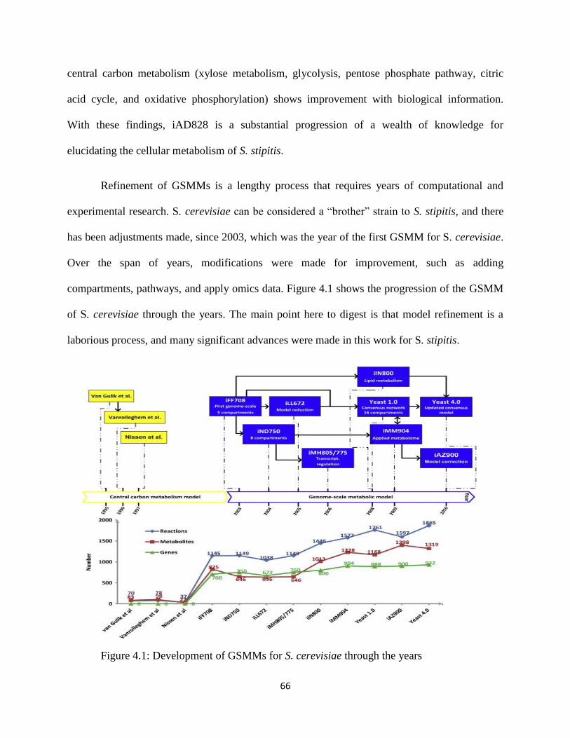
66

central carbon metabolism (xylose metabolism, glycolysis, pentose phosphate pathway, citric

acid cycle, and oxidative phosphorylation) shows improvement with biological information.

With these findings, iAD828 is a substantial progression of a wealth of knowledge for

elucidating the cellular metabolism of S. stipitis.

Refinement of GSMMs is a lengthy process that requires years of computational and

experimental research. S. cerevisiae can be considered a “brother” strain to S. stipitis, and there

has been adjustments made, since 2003, which was the year of the first GSMM for S. cerevisiae.

Over the span of years, modifications were made for improvement, such as adding

compartments, pathways, and apply omics data. Figure 4.1 shows the progression of the GSMM

of S. cerevisiae through the years. The main point here to digest is that model refinement is a

laborious process, and many significant advances were made in this work for S. stipitis.

Figure 4.1: Development of GSMMs for S. cerevisiae through the years

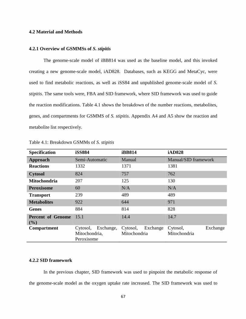
67

4.2 Material and Methods

4.2.1 Overview of GSMMSs of S. stipitis

The genome-scale model of iBB814 was used as the baseline model, and this invoked

creating a new genome-scale model, iAD828. Databases, such as KEGG and MetaCyc, were

used to find metabolic reactions, as well as iSS84 and unpublished genome-scale model of S.

stipitis. The same tools were, FBA and SID framework, where SID framework was used to guide

the reaction modifications. Table 4.1 shows the breakdown of the number reactions, metabolites,

genes, and compartments for GSMMS of S. stipitis. Appendix A4 and A5 show the reaction and

metabolite list respectively.

Table 4.1: Breakdown GSMMs of S. stipitis

Specification iSS884 iBB814 iAD828

Approach Semi-Automatic Manual Manual/SID framework

Reactions 1332 1371 1381

Cytosol 824 757 762

Mitochondria 207 125 130

Peroxisome 60 N/A N/A

Transport 239 489 489

Metabolites 922 644 971

Genes 884 814 828

Percent of Genome

(%)

15.1 14.4 14.7

Compartment Cytosol, Exchange,

Mitochondria,

Peroxisome

Cytosol, Exchange

Mitochondria

Cytosol, Exchange

Mitochondria

4.2.2 SID framework

In the previous chapter, SID framework was used to pinpoint the metabolic response of

the genome-scale model as the oxygen uptake rate increased. The SID framework was used to

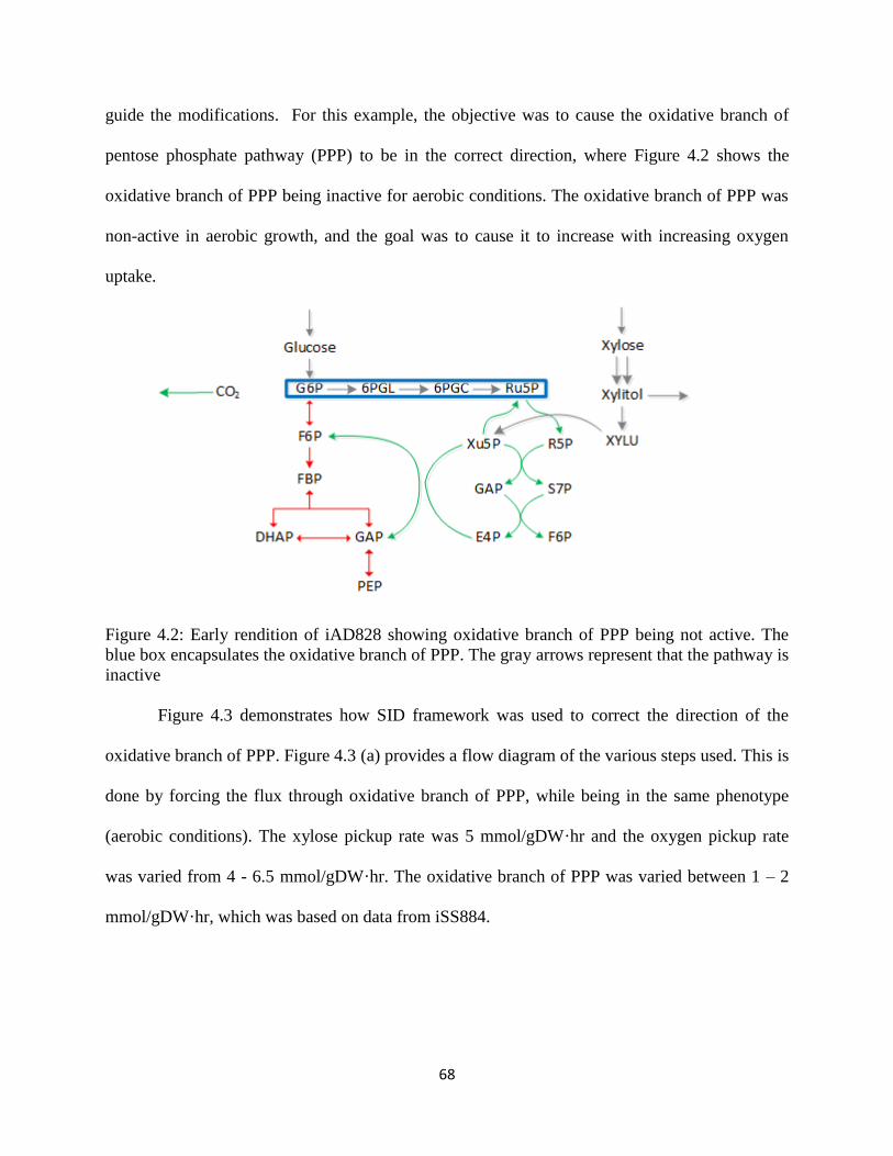
68

guide the modifications. For this example, the objective was to cause the oxidative branch of

pentose phosphate pathway (PPP) to be in the correct direction, where Figure 4.2 shows the

oxidative branch of PPP being inactive for aerobic conditions. The oxidative branch of PPP was

non-active in aerobic growth, and the goal was to cause it to increase with increasing oxygen

uptake.

Figure 4.2: Early rendition of iAD828 showing oxidative branch of PPP being not active. The

blue box encapsulates the oxidative branch of PPP. The gray arrows represent that the pathway is

inactive

Figure 4.3 demonstrates how SID framework was used to correct the direction of the

oxidative branch of PPP. Figure 4.3 (a) provides a flow diagram of the various steps used. This is

done by forcing the flux through oxidative branch of PPP, while being in the same phenotype

(aerobic conditions). The xylose pickup rate was 5 mmol/gDW·hr and the oxygen pickup rate

was varied from 4 - 6.5 mmol/gDW·hr. The oxidative branch of PPP was varied between 1 – 2

mmol/gDW·hr, which was based on data from iSS884.

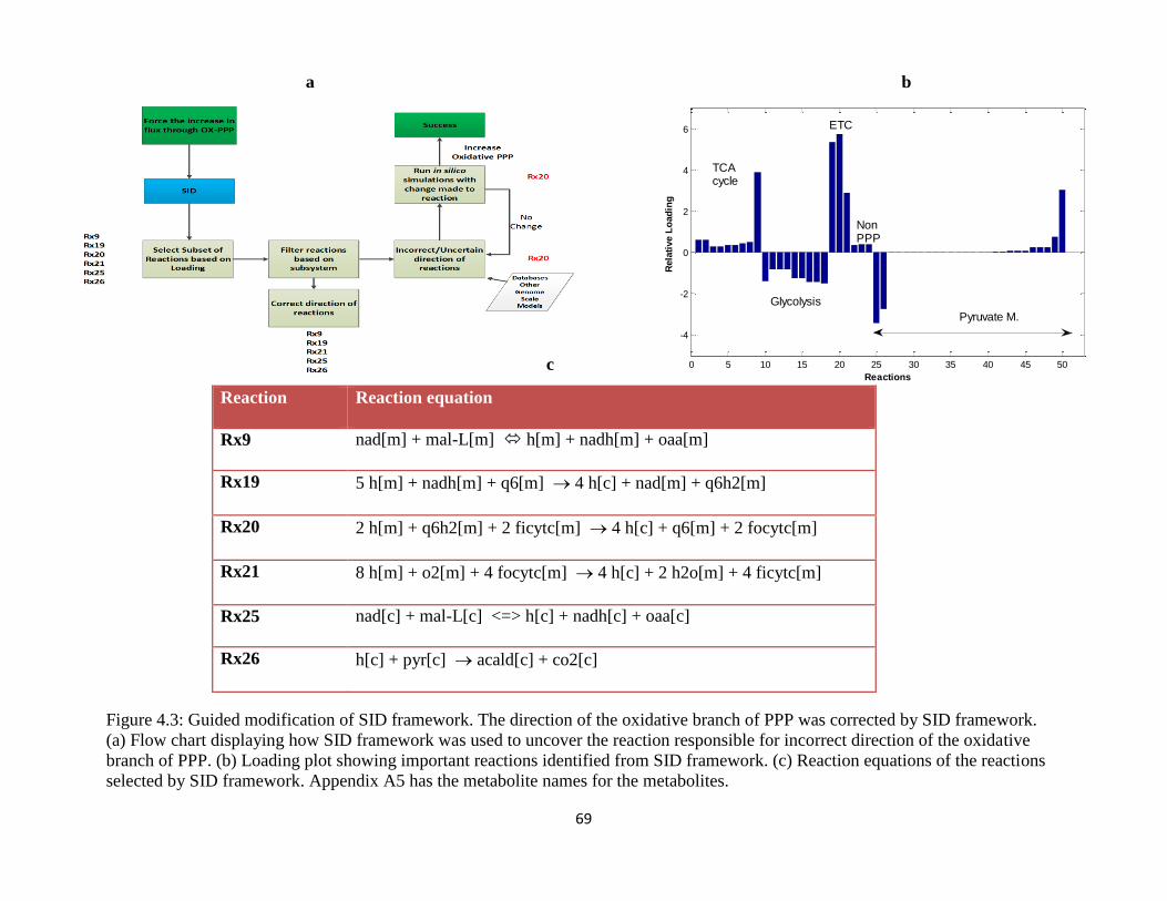
69

Figure 4.3: Guided modification of SID framework. The direction of the oxidative branch of PPP was corrected by SID framework.

(a) Flow chart displaying how SID framework was used to uncover the reaction responsible for incorrect direction of the oxidative

branch of PPP. (b) Loading plot showing important reactions identified from SID framework. (c) Reaction equations of the reactions

selected by SID framework. Appendix A5 has the metabolite names for the metabolites.

Reaction Reaction equation

Rx9 nad[m] + mal-L[m] h[m] + nadh[m] + oaa[m]

Rx19 5 h[m] + nadh[m] + q6[m] 4 h[c] + nad[m] + q6h2[m]

Rx20 2 h[m] + q6h2[m] + 2 ficytc[m] 4 h[c] + q6[m] + 2 focytc[m]

Rx21 8 h[m] + o2[m] + 4 focytc[m] 4 h[c] + 2 h2o[m] + 4 ficytc[m]

Rx25 nad[c] + mal-L[c] <=> h[c] + nadh[c] + oaa[c]

Rx26 h[c] + pyr[c] acald[c] + co2[c]

a b

c 0 5 10 15 20 25 30 35 40 45 50

-4

-2

0

2

4

6

Reactions

Rela

tive L

oad

ing

TCAcycle

NonPPP

ETC

Glycolysis

Pyruvate M.

70

Next, the reactions were filtered out based on whether they were moving in the correct or

incorrect direction. Figure 4.3 (b) displays the reaction loadings for the main subsystems, where

Figure 4.3 (c) shows the reactions that have the highest loading value. Reactions in the correct

direction involved the glycolysis pathway, electron transport chain, exchange, and pyruvate

metabolism. One reaction (Rx20) was selected for the incorrect direction, which is cytosolic

malate dehydrogenase, where the literature shows it is favored in the forward direction. When

the direction of this reaction is blocked, and simulations are run under aerobic conditions, this

results in the oxidative branch of PPP now being activated and in the correct direction. Reactions

can be added to the metabolic model by metabolic databases and genome-scale models of

analogous strains. For example, a main focus of iAD828 was the production of xylitol. It was

decided to use sensitivity analysis on the model to detect, which metabolite played a role in

xylitol production by changing the amount in the objective function. GMP was identified to be

an essential metabolite for xylitol production. Next, the specific reactions were selected from the

subsystems that contained GMP, such as the purine metabolism, and subsystems that were

impacted from the GMP containing subsystems, like PPP. Therefore reactions from metabolic

databases (KEGG), and other genome-scale models (iSS884, unpublished S. stipitis model, and

S. cerevisiae, etc) were selected and implemented into the model. If the modification of the

reaction causes no affect then the steps are looped back.

Tables 4.2-4.4 shows the reactions that were modified, deleted, and added, respectively in

iAD828. There were 13 reactions that were modified. RXm 1 -3 changes occurred in complex I,

III and IV of the electron transport change, where the protons were balanced. RXm 4 - 6

reversible reaction was blocked to ensure the TCA cycle was moving in the proper direction. As

mentioned early, malate dehydrogenase, RXm 7, when blocked resulted in the oxidative branch

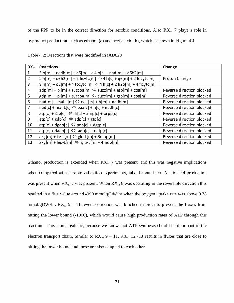
71

of the PPP to be in the correct direction for aerobic conditions. Also RXm 7 plays a role in

byproduct production, such as ethanol (a) and acetic acid (b), which is shown in Figure 4.4.

Table 4.2: Reactions that were modified in iAD828

Ethanol production is extended when RXm 7 was present, and this was negative implications

when compared with aerobic validation experiments, talked about later. Acetic acid production

was present when RXm 7 was present. When RXm 8 was operating in the reversible direction this

resulted in a flux value around -999 mmol/gDW·hr when the oxygen uptake rate was above 0.78

mmol/gDW·hr. RXm 9 – 11 reverse direction was blocked in order to prevent the fluxes from

hitting the lower bound (-1000), which would cause high production rates of ATP through this

reaction. This is not realistic, because we know that ATP synthesis should be dominant in the

electron transport chain. Similar to RXm 9 – 11, RXm 12 -13 results in fluxes that are close to

hitting the lower bound and these are also coupled to each other.

RXm Reactions Change

1 5 h[m] + nadh[m] + q6[m] -> 4 h[c] + nad[m] + q6h2[m]

Proton Change 2 2 h[m] + q6h2[m] + 2 ficytc[m] -> 4 h[c] + q6[m] + 2 focytc[m]

3 8 h[m] + o2[m] + 4 focytc[m] -> 4 h[c] + 2 h2o[m] + 4 ficytc[m]

4 adp[m] + pi[m] + succoa[m] succ[m] + atp[m] + coa[m] Reverse direction blocked

5 gdp[m] + pi[m] + succoa[m] succ[m] + gtp[m] + coa[m] Reverse direction blocked

6 nad[m] + mal-L[m] oaa[m] + h[m] + nadh[m] Reverse direction blocked

7 nad[c] + mal-L[c] oaa[c] + h[c] + nadh[c] Reverse direction blocked

8 atp[c] + r5p[c] h[c] + amp[c] + prpp[c] Reverse direction blocked

9 atp[c] + gdp[c] adp[c] + gtp[c] Reverse direction blocked

10 atp[c] + dgdp[c] adp[c] + dgtp[c] Reverse direction blocked

11 atp[c] + dadp[c] adp[c] + datp[c] Reverse direction blocked

12 akg[m] + ile-L[m] glu-L[m] + 3mop[m] Reverse direction blocked

13 akg[m] + leu-L[m] glu-L[m] + 4mop[m] Reverse direction blocked

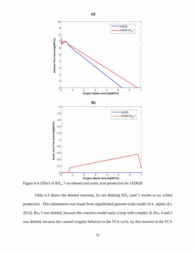
72

Figure 4.4: Effect of RXm 7 on ethanol and acetic acid production for iAD828

Table 4.3 shows the deleted reactions, by not deleting RXd 1and 2 results in no xylitol

production. This information was found from unpublished genome-scale model of S. stipitis (Li,

2012). Rxd 3 was deleted, because this reaction would cause a loop with complex II. Rxd 4 and 5

was deleted, because this caused irregular behavior in the TCA cycle, by this reaction in the TCA

(a)

(b)

0 1 2 3 4 5 6 70

1

2

3

4

5

6

7

8

9

10

Oxygen Uptake (mmol/gDW*hr)

Eth

an

ol

Flu

x (

mm

ol/

gD

W*h

r)

iAD828

iAD828 RXm

7

0 1 2 3 4 5 6 70

0.2

0.4

0.6

0.8

1

1.2

1.4

1.6

1.8

2

Oxygen Uptake (mmol/gDW*hr)

Aceti

c A

cid

Flu

x (

mm

ol/

gD

W*h

r)

iAD828

iAD828 RXm

7

73

cycle (mitochondria) by blocked. Deleting RXd 6 enhanced the strength of iAD828, because

validation experiments that were taken from iBB814 were changed from incorrect to correct,

these results will be presented later.

Table 4.3: Reactions deleted from iAD828

RXd Reactions Reason

1 abt-D[e] -> Impact on xylitol

2 abt-L[e] ->

3 fum[c] + fadh2[m] -> succ[c] + fad[m] Causes loop

4 fum[c] + h2o[c] -> mal-L[c] Branch TCA cycle

5 nadp[c] + icit[c] -> nadph[c] + co2[c] + akg[c] TCA cycle

6 glu5sa[m] + h2o[m] + nadp[m] -> glu-L[m] + 2 h[m] + nadph[m] Improved model prediction

7 h[c] + nadph[c] + akg[c] + nh4[c] -> nadp[c] + h2o[c] + glu-L[c] Improved model prediction

Table 4.4 displays the reactions that were added to the model, where the RXA 1 and 2

were shown to have an impact on xylitol, where RXA 1 was taken from iSS884 and RXA 2 was

identified in metabolic database for S. stipitis, both were taken from the purine metabolism. RXA

3 also had an effect on xylitol production, where this reaction was located in the mitochondria in

iBB814. One of the problems that were encountered was matching the model results to the

experimental validation results, under aerobic conditions, when both glucose and xylose was

used as the substrate. The validation experiment showed no ethanol production, where iAD828

was producing ethanol. This was due to having not enough NADH being oxidized in the cytosol.

An oxidation reaction that alleviates the amount of NADH in the cytosol was glutamate

dehydrogenase, which uses akg[c]. RXA 4, 8, and 11 were reactions that played as a source for

akg[c] production. RXA 4 operates in the reverse direction, RXA 8 is a mitochondria transport

reaction that proceeds in the forward direction, and RXA 11 is a mitochondria transport reaction

that operates in the reverse direction.

74

Table 4.4: Reactions added to iAD828

RXA Reactions Reason

1 prpp[c] + gua[c] <=> ppi[c] + gmp[c]

Impact on xylitol 2 h2o[c] + gsn[c] <=> nh4[c] + xtsn[c]

3 ser-L[c] + 0.01 cdpdag[c] <=> 0.01 ps[c] + cmp[c]

4 ala-L[c] + akg[c] <=> pyr[c] + glu-L[c] Impact on ethanol – minimal

5 glu-L[m] + h[m] -> co2[m] + 4abut[m]

Succinate bypass 6 akg[m] + 4abut[m] <=> glu-L[m] + succsal[m]

7 h2o[m] + nadp[m] + succsal[m] -> succ[m] + 2 h[m] + nadph[m]

8 akg[m] + mal-L[c] <=> akg[c] + mal-L[m]

Impact on ethanol and xylitol 9 h[c] + nadh[c] + glu-L[c] <=> 2 h2o[c] + nad[c] + 1pyr5c[c]

10 glu-L[m] + h[m] + nadh[m] <=> 2 h2o[m] + nad[m] + 1pyr5c[m]

11 akg[c] + 2oxoadp[m] <=> akg[m] + 2oxoadp[c] Impact on ethanol

12 h2o[c] + ptd1ino[c] <=> 12dgr[c] + mi1p-D[c]

These reactions cause an excess of akg[c] in the model that needs to be consumed, and the model

choses to use glutamate dehydrogenase. Therefore, there is now the validation experiments

match the model results under aerobic condition for both glucose and xylose. The succinate

bypass RXA 5 - 7 was implemented in the model, as an alternative route to produce succinate in

the mitochondria as imposed from the TCA cycle. Another part that added to having successful

matching of the model to the validation experiments were RXA 9 and 10, these reactions were

found in the S. cerevisiae model. RXA 12 played a role in ethanol and xylitol production.

4.2.3 In silico examination and traditional experimental validation

The genome-scale metabolic models were evaluated by flux balance analysis (FBA), in

which the COBRA toolbox (Schellenberger et al., 2011) was used. For all the simulations, the

objective function was biomass growth. The upper limits of xylose and oxygen uptakes were

varied based on the preselected conditions, while the other exchange compounds (NH4+

, H+,

SO42-

, Pi2-

, H2O, Fe2+

) were given the option to enter and exit the network freely, with upper and

75

lower bounds of -1000 to 1000 mmol/gDW·hr. The final metabolic products (CO2, ethanol,

acetic acid, etc.) were allowed to exit the system freely, where the reaction flux was constrained

to 0 – 1000 mmol/gDW·hr, which prevents product uptake. The growth associated maintenance

energy was set to 2.6 mmol/gDW·hr (Balagurunathan et al., 2012). This setup was applied to all

in silico simulations for both models.

4.3 Results and Discussion

3D plots that varied xylose and oxygen were made for iAD828 for growth, ethanol, and

CO2, which were compared with the published genome-scale metabolic network models of

iSS884 and iBB814. Note that xylitol was only done for iAD828, since iSS884 and iBB814 does

not produce xylitol. SID framework was used to compare iSS84 and iBB814 with the newly

developed model of iAD828, under oxygen-limited and aerobic conditions. The central carbon

metabolism was the focus since it encompasses the significant metabolic behavior and literature

was available. iAD828 had a major improvement compared to the previous models, since xylose

metabolism, glycolysis, oxidative and non-oxidative PPP, TCA cycle, and ETC are now

operating correctly. The same validation experiments that were used in comparing iSS884 and

iBB814 were used to show how iAD828 outperforms the former models. A recently published

paper was used to validate the production of xylitol for iAD828.

4.3.1 Phenotype phase plane analysis

In this analysis, xylose and oxygen uptake rates were chosen as the independent

variables, with each of them varying from 0 – 10 mmol/gDW·hr for the analysis of growth rate,

ethanol and CO2. Since xylitol is only produced under oxygen-limited condition, iAD828 results

were compared with the published models of iSS884 and iBB814.

76

02

46

810

0

2

4

6

8

100

0.2

0.4

0.6

0.8

1

Xylose uptake Oxygen uptake

Gro

wth

ra

te

iSS884

(a)

02

46

810

0

2

4

6

8

100

0.2

0.4

0.6

0.8

1

Xylose uptake Oxygen uptake

Gro

wth

ra

te

iBB814

iAD828

02

46

810

0

2

4

6

8

100

0.2

0.4

0.6

0.8

1

Xylose uptake Oxygen uptake

Gro

wth

ra

te

77

24

6

810

02

46

8100

5

10

15

Xylose uptakeOxygen uptake

Eth

an

ol

iSS884

(b)

24

6

810

02

46

8100

5

10

15

Xylose uptakeOxygen uptake

Eth

an

ol

iBB814

iAD828

02

46

810

02

46

8100

5

10

15

Xylose uptake Oxygen uptake

Eth

an

ol

78

02

46

810

0

2

4

6

8

100

5

10

15

20

Xylose uptake Oxygen uptake

CO

2

iSS884 (c)

02

46

810

0

2

4

6

8

100

5

10

15

20

Xylose uptake Oxygen uptake

CO

2

iBB814

02

46

810

0

2

4

6

8

100

5

10

15

20

Xylose uptake Oxygen uptake

CO

2

02

46

810

0

2

4

6

8

100

5

10

15

20

Xylose uptake Oxygen uptake

CO

2

iAD828

79

Figure 4.5: 3D product profiles: (a) Growth rate, (b) Ethanol, (c) CO2, (d) Xylitol

Figure 4.5 (a) show how cell growth rate is affected by different substrate uptake rates, where the

differently colored regions represent different growth behaviors. Overall, cell growth profiles

predicted by iSS884 and iBB814 are similar to each other, except that the growth rate predicted

by iBB814 is significantly lower than iSS884 and iAD828. Figure 4.5 (b) shows the ethanol

profiles for the models, where both iSS884 and iAD828 predicts a larger area of zero ethanol

production, which is shown as the green phenotype. Figure 4.5 (c) shows the CO2 production

profiles for the models, where iSS884 and iAD828 have great similarity. Figure 4.5 (d) shows

the xylitol production profile for iAD828, where the xylitol production rate only occurs under

oxygen-limited conditions.

4.3.2 Model comparison through the SID framework

SID framework was carried out on iSS884, iBB814, and iAD828, where 2D phenotype

phase plots were generated to compare the distribution of the phenotypes, which is shown in

01

2

34

5

00.10.20.30.40.50.60.70.80.91

0

0.1

0.2

0.3

0.4

0.5

Xylose uptake

Oxygen uptake

Xy

lito

l

iAD828

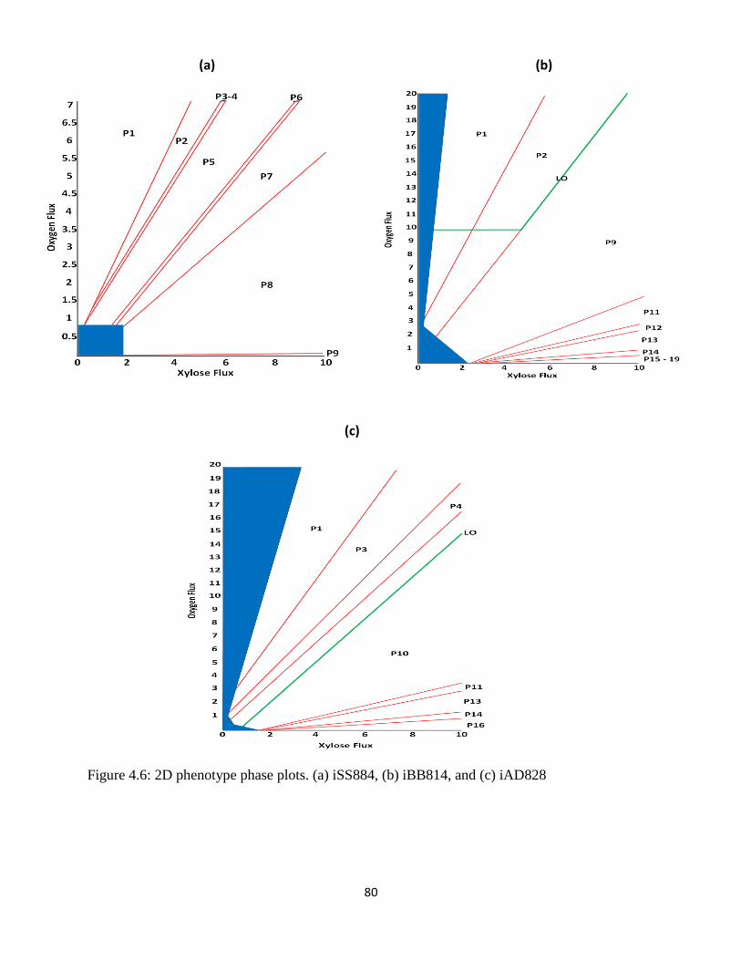
80

Figure 4.6: 2D phenotype phase plots. (a) iSS884, (b) iBB814, and (c) iAD828

(b) (a)

(c)

81

Figure 4.6 (a) – (c) respectively. The phenotypes are labeled as P and are ordered by the most

oxygen plentiful to least (aerobic to oxygen-limited). The blue regions represent infeasible

regions. iSS884 has the fewest phenotypes, where P1 and P8 encompass the majority of the

metabolic behavior. Certain phenotypes change only minimally, which is why they are

combined, for example, P3 and P4 in iSS884. Moving to iBB814, P9 is the most dominant

phenotype in terms of representing the phenotypic space, where P1 and P2 ahave large

phenotypic regions. As the oxygen pickup rate decreases from P2, there are a lot of phenotypes

that occupy very minimal metabolic behavior, which are omitted from the plot, such P3 – P8.

The infeasible region of iBB814 is larger and infeasible regions exist in the aerobic region.

iAD828 has similar amount of phenotypes compared to iBB814, where it has similar features as

iBB814 in terms of the infeasible region and lower oxygen region phenotypes. The LO for

iSS884 always hits the lower bound for the oxygen uptake (-1000 mmol/gDW·hr: maximum

uptake) and that is why it is not shown in the plot, thus iSS884 has a serious error in the

phenotypic makeup. The LO for iBB814, hits an oxygen pickup rate of 10 mmol/gDW·hr for a

xylose pickup range of 1.8 to 4.69 mmol/gDW·hr, then the oxygen pickup rate increases for

xylose pickup rates above 4.69 mmol/gDW·hr, which is designated by the green line and labeled

LO. The LO for iAD828 has the correct response, since it the LO should been a diagonal line.

LO is defined as the optimal relationship between the xylose and oxygen uptake rates.

The first condition that was investigated was under oxygen-limited condition, where the

results are shown in Figure 4.7. The oxygen pick up rate varied from 0.11 – 0.15 mmol/gDW·hr.

This correlated with the following phenotypes: P8 for iSS884, P17 for iBB814, and P17 for

iAD828. Both branches of the PPP, oxidative and non-oxidative for all the models are correctly

regulated. iSS884 and iAD828 have the glycolysis pathway downregulated, while iBB814 is

82

upregulated, where the literature is in accordance with iSS884 and iAD828 (Skoog and Hahn-

Hägerdal, 1990). The xylose metabolism is affected differently in iAD828, due to the production

of xylitol, which is shown to be a key byproduct under oxygen-limited condition. iSS884 has

irregular behavior in ethanol production, because it not only occurs in two compartments, but

there is also a reaction that proceeds in the wrong direction, which consumes ethanol. That is

shown in Figure 4.7 by the thick red line with NAD above it, signifying that it utilizes this type

of cofactor. The reaction that produces ethanol in the cytosol uses NADPH, but there is not much

change. The major variation of ethanol production occurs in the mitochondria, where this

reaction is upregulated. As noted in the previous chapter that both reactions in the cytosol are

close to hitting the upper bound, above 990 mmol/gDW·hr.

One place this unusual behavior is traced to is that malate dehydrogenase is operating in

reverse direction in the TCA cycle, and is very heavily downregulated, which is directly

connected to the high amount of oxaloacetate (oaa) that is being transported from the cytosol.

The irregular behavior of ethanol production and reactions connected to malate dehydrogenase in

the mitochondria show iSS884 inability to have a biologically sound redox balance. iAD828

follows iSS884 in that ethanol production is declining, while iBB814 has increasing ethanol

production. All models have a branched TCA cycle; however there are distinctions between the

models. iSS884 and iAD828 branch at the same point, however there is irregular behavior in

iSS884 and iBB814, where malate dehydrogenase is operating in the reverse direction. Lastly,

the electron transport chain of iBB814 and iAD828 share similar characteristics, though iBB814

has a low upregulation of complex I compared to iAD828. As previous described, iSS884 has

biologically irregular behavior in the electron transport chain.

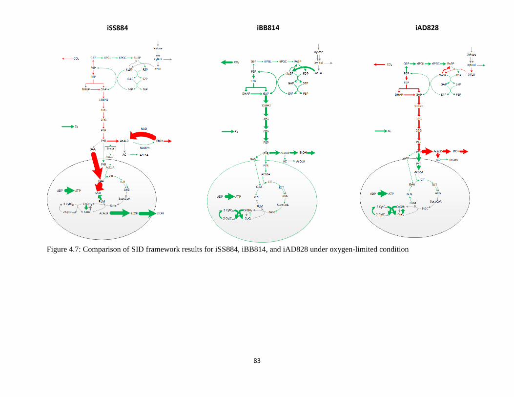
83

Figure 4.7: Comparison of SID framework results for iSS884, iBB814, and iAD828 under oxygen-limited condition

iAD828 iBB814 iSS884

84

The next phenotype that was examined, P16, dealt with a decrease in xylitol production

rate, where the oxygen uptake rate was varied 0.161 – 0.385 mmol/gDW·hr, where the results

are shown in Figure 4.8 This phenotype results in a major shift in the direction of regulation

glycolysis, and the regulation direction of the byproducts of ethanol and carbon dioxide. All the

remaining central carbon metabolism pathways stay in the same regulation direction as P17. The

upregulation oxidative branch of the pentose phosphate pathway for P16 has diminished in

comparison to P17.

The next phenotype P14 that was investigated was still under oxygen-limited condition,

but now the xylitol production is eliminated, which is shown in Figure 4.9. The oxygen uptake

rate was varied between 0.67 – 0.90 mmol/gDW·hr.

Figure 4.8: SID framework results of P16 for iAD828

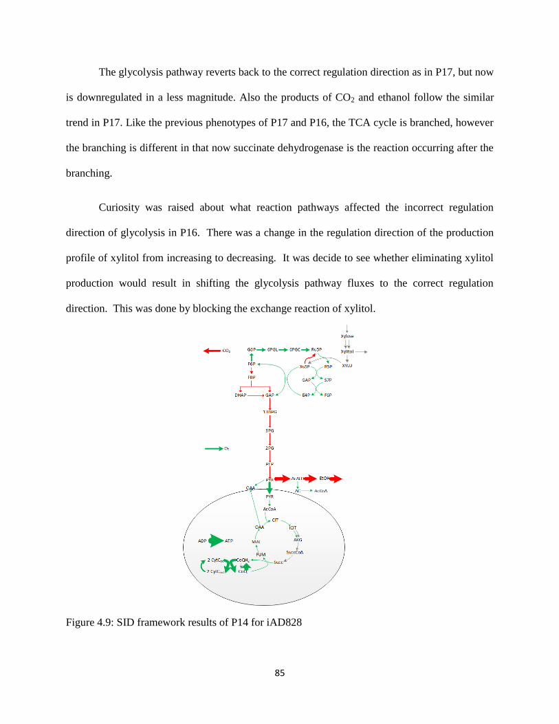
85

The glycolysis pathway reverts back to the correct regulation direction as in P17, but now

is downregulated in a less magnitude. Also the products of CO2 and ethanol follow the similar

trend in P17. Like the previous phenotypes of P17 and P16, the TCA cycle is branched, however

the branching is different in that now succinate dehydrogenase is the reaction occurring after the

branching.

Curiosity was raised about what reaction pathways affected the incorrect regulation

direction of glycolysis in P16. There was a change in the regulation direction of the production

profile of xylitol from increasing to decreasing. It was decide to see whether eliminating xylitol

production would result in shifting the glycolysis pathway fluxes to the correct regulation

direction. This was done by blocking the exchange reaction of xylitol.

Figure 4.9: SID framework results of P14 for iAD828

86

Removing xylitol production does not cause the glycolysis pathway to change to the correct

response. One interesting change that was found when blocking the xylitol production was that

now the oxidative branch of PPP was downregulated. This brought about possible explanation,

that in P16 the oxidative branch of the PPP was reduced in activation. This propagated in silico

experiments that forced the upregulation of the oxidative branch to be above the optimized

solution. This in turn caused the xylitol production to be decreased to zero. The region where

xylitol production was zero resulted in glycolysis now being in the correct regulation direction.

Looking at the loading values for the oxidative branch and non-oxidative branch of PPP, we find

that the loading value is always higher for the oxidative branch when the glycolysis pathway is in

the correct direction. A final study was conducted on P16 that lowers the upregulation of the

non-oxidative branch of PPP to be less than the oxidative branch of PPP. The results are

agreement with what was observed before, which brought about glycolysis in the correct

regulation direction. It is evident from this analysis that glycolysis, oxidative branch of PPP, and

non-oxidative branch of PPP are correlated.

The next phenotype P10 in iAD828 that was examined was in the aerobic regime, and

this was compared with iSS884 (P5) and iBB814 (P9), which is seen in Figure 4.10. First

looking at the oxidative branch of PPP, iSS884 and iAD828 have it in the correct regulation

direction, while iBB814 does not have the reactions affected. The next subsystems that were

investigated were glycolysis and the non-oxidative branch, and all models have correct

responses. Turning to the TCA cycle, we see that iAD828 is the only model where the TCA

cycle is fully activated; both iSS884 and iBB814 have fumarase reaction inactivated, thus

causing a branch. Also in iSS884, malate dehydrogenase is heavily upregulated compared to the

other TCA cycle reactions that are all on the same magnitude. As stated before, the electron

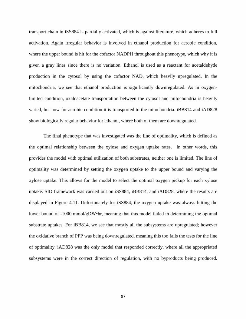
87

transport chain in iSS884 is partially activated, which is against literature, which adheres to full

activation. Again irregular behavior is involved in ethanol production for aerobic condition,

where the upper bound is hit for the cofactor NADPH throughout this phenotype, which why it is

given a gray lines since there is no variation. Ethanol is used as a reactant for acetaldehyde

production in the cytosol by using the cofactor NAD, which heavily upregulated. In the

mitochondria, we see that ethanol production is significantly downregulated. As in oxygen-

limited condition, oxaloacetate transportation between the cytosol and mitochondria is heavily

varied, but now for aerobic condition it is transported to the mitochondria. iBB814 and iAD828

show biologically regular behavior for ethanol, where both of them are downregulated.

The final phenotype that was investigated was the line of optimality, which is defined as

the optimal relationship between the xylose and oxygen uptake rates. In other words, this

provides the model with optimal utilization of both substrates, neither one is limited. The line of

optimality was determined by setting the oxygen uptake to the upper bound and varying the

xylose uptake. This allows for the model to select the optimal oxygen pickup for each xylose

uptake. SID framework was carried out on iSS884, iBB814, and iAD828, where the results are

displayed in Figure 4.11. Unfortunately for iSS884, the oxygen uptake was always hitting the

lower bound of -1000 mmol/gDW•hr, meaning that this model failed in determining the optimal

substrate uptakes. For iBB814, we see that mostly all the subsystems are upregulated; however

the oxidative branch of PPP was being downregulated, meaning this too fails the tests for the line

of optimality. iAD828 was the only model that responded correctly, where all the appropriated

subsystems were in the correct direction of regulation, with no byproducts being produced.

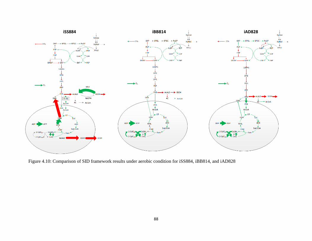
88

Figure 4.10: Comparison of SID framework results under aerobic condition for iSS884, iBB814, and iAD828

iSS884 iAD828 iBB814

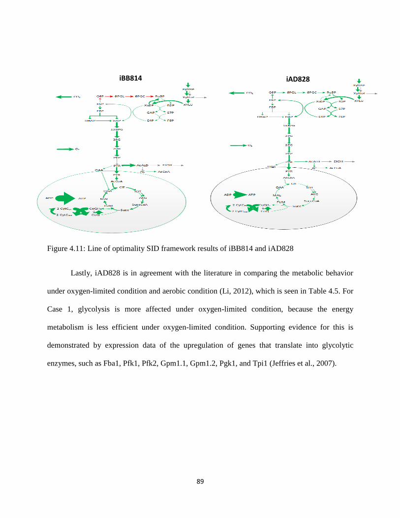
89

Figure 4.11: Line of optimality SID framework results of iBB814 and iAD828

Lastly, iAD828 is in agreement with the literature in comparing the metabolic behavior

under oxygen-limited condition and aerobic condition (Li, 2012), which is seen in Table 4.5. For

Case 1, glycolysis is more affected under oxygen-limited condition, because the energy

metabolism is less efficient under oxygen-limited condition. Supporting evidence for this is

demonstrated by expression data of the upregulation of genes that translate into glycolytic

enzymes, such as Fba1, Pfk1, Pfk2, Gpm1.1, Gpm1.2, Pgk1, and Tpi1 (Jeffries et al., 2007).

iAD828 iBB814

90

Table 4.5: Metabolic artifacts to further validate iAD828. Case 1 shows glycolytic genes: Gpm -

Phosphoglycerate mutase, Pfk - Phosphofructokinase, Pgk - Phosphoglycerate kinase, Fba -

Fructose-1,6-bisphosphate aldolase, Tpi - Triose Phosphate Isomerase.

Case 1

Genes Oxygen -L Aerobic

Gpm1.1,2 7.32 6.79

Pfk1,2 2.92 2.55

Pgk1 7.40 6.95

Fba1 2.92 2.55

Tpi1 2.92 2.54

Case 2

Reactions Oxygen-L Aerobic

Fatty acid synthase (n-C10:0) 2.94 x 10-3 0

Fatty acid synthase (n-C12:0) 2.85 x 10-3 0

Fatty acid synthase (n-C14:0) 2.31 x 10-3 0

Fatty-acyl-CoA synthase (n-

C16:0CoA) 2.03 x 10-3 0

Fatty acid synthase (n-C18:0) 8.10 x 10-4 0

Case 3

Reactions Oxygen-L Aerobic

Citrate -> α-Ketoglutarate 0.08 0.61

α-Ketoglutarate -> Succinate 0.00 0.26

Succinate -> Fumarate 0.00 0.37

Fumarate -> Oxaloacetate 0.03 0.47

This was simulated by collecting the fluxes under oxygen-limited and aerobic for the glycolytic

reactions that were impacted. As shown in Table 4.5, the flux values are higher under oxygen-

limited condition, which agrees with the literature. For Case 2, the literature shows that fatty acid

synthesis transcripts are higher under oxygen-limited condition. In silico simulations were run in

iAD828 that demonstrated this by only having fatty acid synthesis reactions active under

oxygen-limited condition (Jeffries, 2006). Moving to Case 3, the TCA cycle should be utilized

more under aerobic condition, due to being the most efficient pathway for ATP production.

iAD828 validates this result by having a higheer flux under aerobic condition (Li, 2012).

4.3.3 Validation experiments

To further confirm iAD828, the same validation experiments that were carried out in

Chapter 3 are shown here. Validation experiments that were taking from the independent data

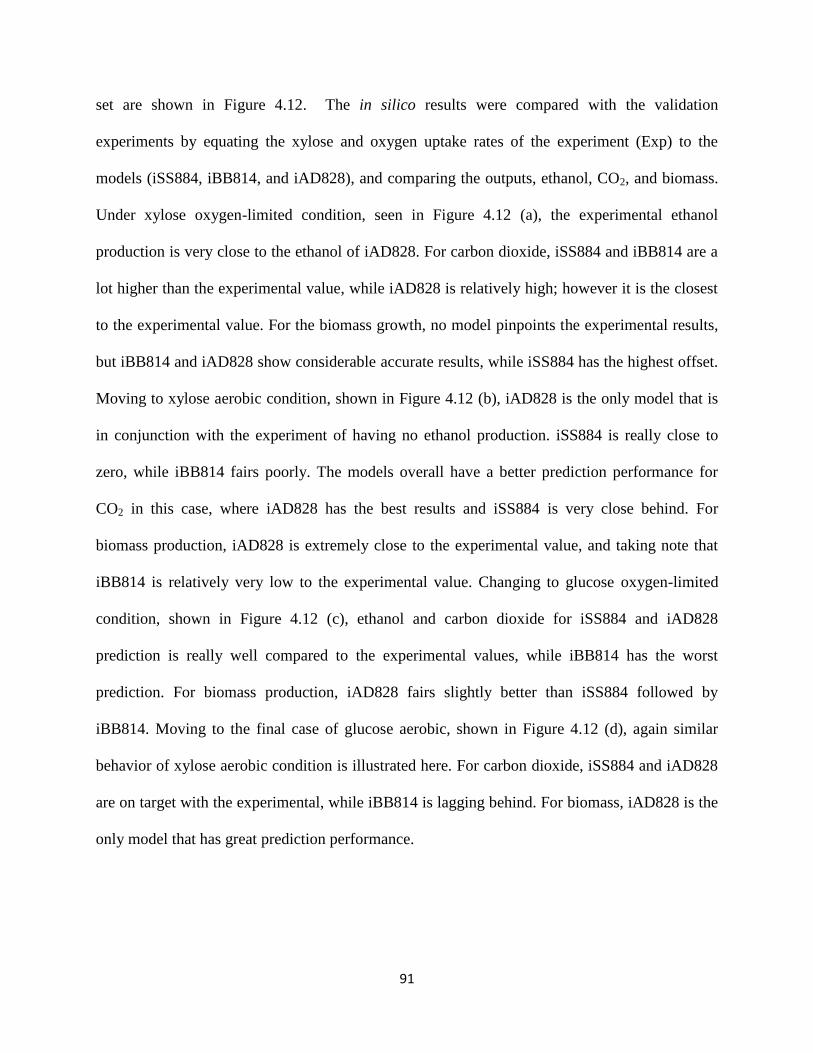
91

set are shown in Figure 4.12. The in silico results were compared with the validation

experiments by equating the xylose and oxygen uptake rates of the experiment (Exp) to the

models (iSS884, iBB814, and iAD828), and comparing the outputs, ethanol, CO2, and biomass.

Under xylose oxygen-limited condition, seen in Figure 4.12 (a), the experimental ethanol

production is very close to the ethanol of iAD828. For carbon dioxide, iSS884 and iBB814 are a

lot higher than the experimental value, while iAD828 is relatively high; however it is the closest

to the experimental value. For the biomass growth, no model pinpoints the experimental results,

but iBB814 and iAD828 show considerable accurate results, while iSS884 has the highest offset.

Moving to xylose aerobic condition, shown in Figure 4.12 (b), iAD828 is the only model that is

in conjunction with the experiment of having no ethanol production. iSS884 is really close to

zero, while iBB814 fairs poorly. The models overall have a better prediction performance for

CO2 in this case, where iAD828 has the best results and iSS884 is very close behind. For

biomass production, iAD828 is extremely close to the experimental value, and taking note that

iBB814 is relatively very low to the experimental value. Changing to glucose oxygen-limited

condition, shown in Figure 4.12 (c), ethanol and carbon dioxide for iSS884 and iAD828

prediction is really well compared to the experimental values, while iBB814 has the worst

prediction. For biomass production, iAD828 fairs slightly better than iSS884 followed by

iBB814. Moving to the final case of glucose aerobic, shown in Figure 4.12 (d), again similar

behavior of xylose aerobic condition is illustrated here. For carbon dioxide, iSS884 and iAD828

are on target with the experimental, while iBB814 is lagging behind. For biomass, iAD828 is the

only model that has great prediction performance.

92

The other quantitative experiment was from iSS884 paper, which is displayed in Figure

4.13, where the same comparison procedure is used. These validation experiments deal with

very low oxygen conditions at less than 1 mmol/gDW·hr, compared to the independent set where

the levels were much higher. Beginning with the lowest oxygen uptake rate, which is displayed

in Figure 4.13 (a), overall the models perform very similar for ethanol and CO2, but there is a

distinction of iBB814 from iSS884 and iAD828 in terms of growth rate, were iSS884 and

iAD828 are more accurate. The similar trend is observed in Figure 4.13 (b) and (c).

Switching to qualitative validation experiments, where deleting the original entry reaction

into the PPP and configuring an alternative route to PPP by genetically engineering the pathway

brought about zero ethanol production. The schematic diagram is shown in Figure 4.14 (a). The

results of the experimental and comparison of the GSMMS of iSS884, iBB814, and iAD828 are

shown in Figure 4.14 (b). iAD828 has complete agreement with the experimental results. The

ethanol production for iBB814 can be misleading; it is only nonzero at the initial point of a zero

oxygen uptake rate, and not under very low oxygen conditions. iSS884 has the worst

performance, where has nonzero production rates of ethanol. The similarities between iAD828

and iBB814 are due to iAD828 being derived from iBB814.

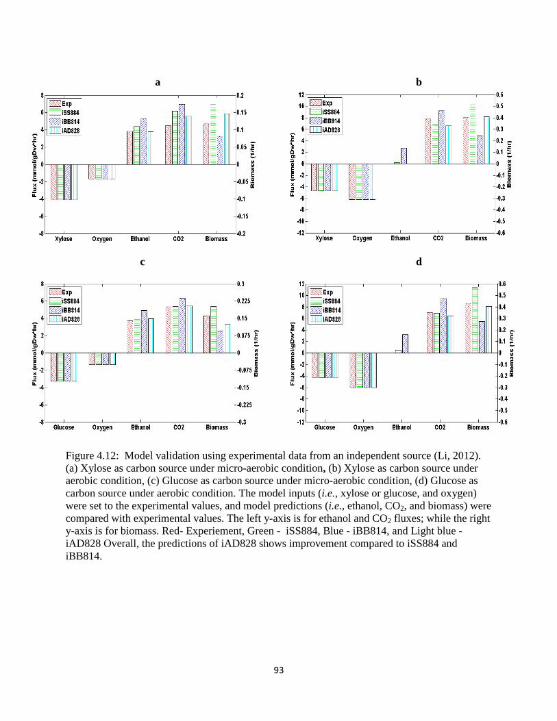
93

Figure 4.12: Model validation using experimental data from an independent source (Li, 2012).

(a) Xylose as carbon source under micro-aerobic condition, (b) Xylose as carbon source under

aerobic condition, (c) Glucose as carbon source under micro-aerobic condition, (d) Glucose as

carbon source under aerobic condition. The model inputs (i.e., xylose or glucose, and oxygen)

were set to the experimental values, and model predictions (i.e., ethanol, CO2, and biomass) were

compared with experimental values. The left y-axis is for ethanol and CO2 fluxes; while the right

y-axis is for biomass. Red- Experiement, Green - iSS884, Blue - iBB814, and Light blue -

iAD828 Overall, the predictions of iAD828 shows improvement compared to iSS884 and

iBB814.

a b

c d

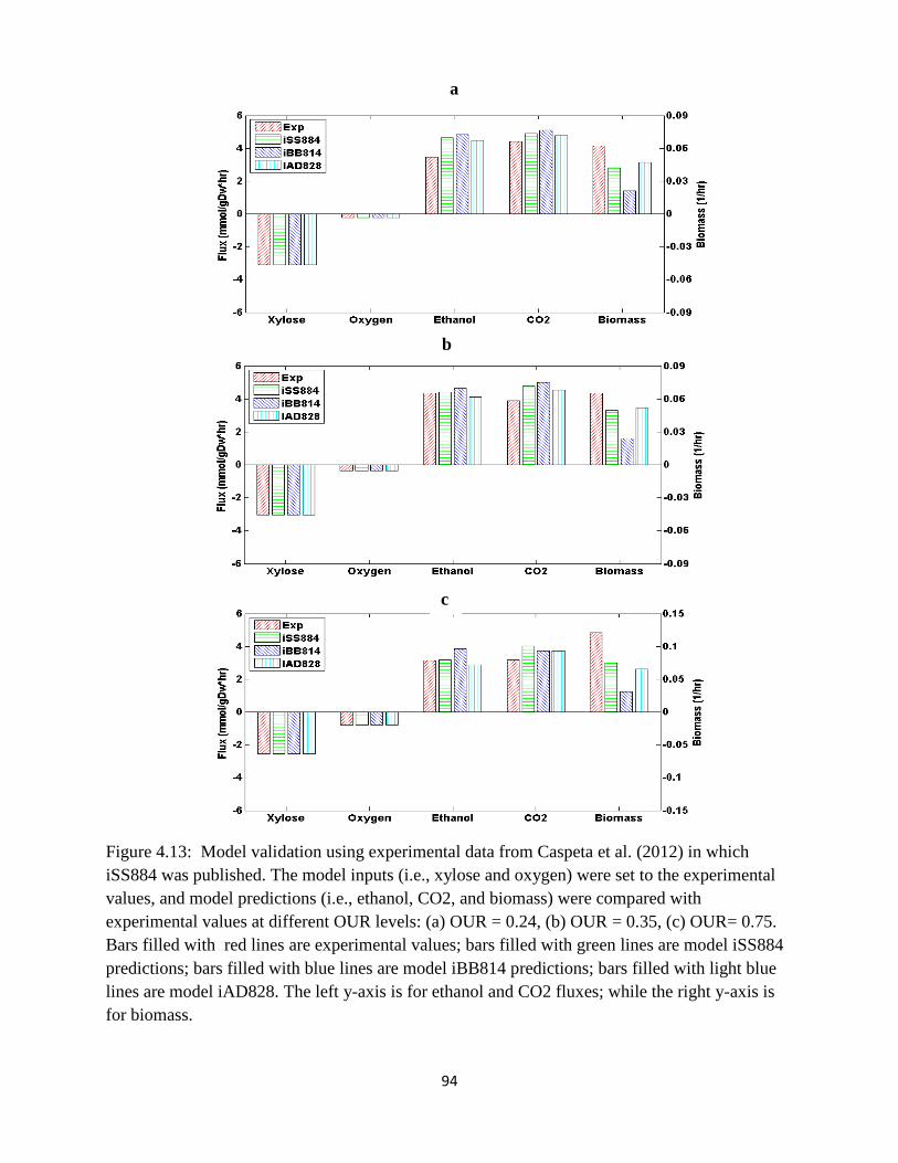
94

Figure 4.13: Model validation using experimental data from Caspeta et al. (2012) in which

iSS884 was published. The model inputs (i.e., xylose and oxygen) were set to the experimental

values, and model predictions (i.e., ethanol, CO2, and biomass) were compared with

experimental values at different OUR levels: (a) OUR = 0.24, (b) OUR = 0.35, (c) OUR= 0.75.

Bars filled with red lines are experimental values; bars filled with green lines are model iSS884

predictions; bars filled with blue lines are model iBB814 predictions; bars filled with light blue

lines are model iAD828. The left y-axis is for ethanol and CO2 fluxes; while the right y-axis is

for biomass.

a

b

c

95

Figure 4.14: Model comparison of the mutant strains of iSS884, iBB814, and iAD828. The

mutant with the alternative route into the pentose phosphate pathway for metabolizing xylose by

deletion of xylulokinase reaction. (a) Schematic diagram of the wild type xylose metabolism

(thin arrows with active xylulokinase reaction (re3)) and mutant with the alternative route (bold

arrows with the deletion of re3); (b) Comparison of ethanol production: EXP is the experimental

results (solid black line), iSS884 (red circle), iBB814 (blue square), and iAD828 (green triangle).

0 0.1 0.2 0.3 0.4 0.5 0.6 0.7 0.8 0.9 1-1

0

1

2

3

4

5

6

7

Oxygen uptake (mmol/gDW*hr)

Eth

an

ol (

mm

ol/g

DW

*hr)

EXP

iSS884

iBB814

iAD828

96

The other qualitative validation experiment was deleting electron transport chain

complexes and classifying the response in different categories of cell growth, the results are

shown in Table 4.6. The symbol - - is complete inhibition, for partial inhibition the symbol is -,

the symbol for negligible is 0, and the symbol for increase is +. Complete inhibition occurred

when the growth rate of the deleted complex(s) was zero. For partial inhibition, this percent

decrease of growth rate was based on the oxygen uptake rate, since at a lower oxygen uptake the

percent decrease diminishes. The paper that was used did not cite an oxygen uptake rate, so

different oxygen uptake rates were run to see if this would result in unusual behavior. The

oxygen uptake rate was set at 2 mmol/gDW·hr and for all the partial inhibition cases the percent

decrease in growth was over 15 %. For the last case, I + del IV, the percent decrease of growth

was 45% and 51 %, for glucose and xylose respectively, which was the highest percent decrease

for all the cases, so even though iAD828 did not reach complete inhibition it is still on the right

track. Overall, iAD828 results supersede the previous models.

Table 4.6: The effects of inhibiting electron transport chain complexes on cell growth for glucose

and xylose: comparison of iSS884 (884) and iBB814 (814) to experimental (Exp) results.

Symbols: complete inhibition (- -), partial inhibition (-), negligible (0), enhanced (+), information

not available (NA). The model predictions that match the experimental results are shaded.

Improvement is made for iAD828 compared to the other models.

Complex

Effect on Growth

Glucose Xylose

Exp iAD828 iSS884 iBB814 Exp iAD828 iSS884 iBB814

I - - - 0 0 - - 0 0

III NA - 0 - - - 0 -

AOX 0 0 - 0 + 0 - 0

IV - - 0 - - - 0 -

IV and

AOX - - - - - - - - - - - - - -

I + del

AOX - - - - - 0 - - - - - 0

I + del

IV - - - 0 - - - - - 0 -

97

The iAD828 was used to reproduce the experimental data for xylitol production. Since

oxygen uptake rate was not provided for in the experiments, thus ethanol yield was matched

between the experiment and model, whereby this was done by changing the oxygen uptake rate

and the xylose reductase (XR) redox ratio. The output that was calculated was xylitol production,

and this was compared with the experimental values, which are shown in Table 4.7. For all the

cases, iAD828 prediction performance of xylitol is very impressive. The results tell us that S.

stipitis adapts to the environment by adjusting the XR redox ratio. Xylose reductase reaction has

two pathways, one uses NADH and the other NADPH. There is not a determined ratio in the

literature between the reactions, however the enzyme activity has been recorded, where the XR

activity ratio was determined to be 2.20.

Table 4.7: Comparison of iAD828 xylitol results to experimental data. YE/S is the ethanol yield,

where xylose is the substrate (S). Xylose reductase (XR) redox ratio and oxygen uptake rate

(OUR) was varied. Minimized the error between ethanol yield of experiment and prediction from

iAD828, then examined the xylitol production of both experimental and prediction.

Other papers have suggested that the NADPH route is more active in terms of enzyme activity.

Nonetheless, it is not clear whether enzyme activity is directly proportional to flux value;

therefore it is not a fair assessment to rely on enzyme activity. The general trend was that the

XR redox ratio increased for increasing ethanol yields. Based on intuition, this trend is

reasonable, since the reaction (xylose dehydrogenase) following utilizes NAD, which if more of

98

the NADH reaction of xylose reductase is taken this means greater amounts of available NAD

for xylose dehydrogenase is present. As a result, abundant NADH is produced from xylose

dehydrogenase and this is provides NADH available for ethanol production. As more carbon

flux is pushed through the NADPH xylose reductase reaction then less NADH is available for

ethanol production, thus less ethanol is produced.

4.3.4 Redox analysis of iAD828

The elucidation of redox balance of S. sitpitis is an important analysis, since it has yet

been established what reactions govern the redox, and currently the understanding is poor. If

understanding of the redox balance is brought to maturity then this will bring about great

potential for successful recombinant strains. iAD828 shows improvement compared to the

previous published model, thus it was used to investigate the redox mechanism for S. sitpitis.

The key redox reactions were determined by examining the loadings from the SID

framework results, where Figure 4.15 displays the relative loading for main redox reaction for

P17. Loadings in the positive direction represent a positive correlation between oxygen uptake

rate, and for the negative direction there is a negative correlation. Table 4.8 shows the

description of the reactions in Figure 4.15, and the starting, ending, and difference of flux values.

There are 3 NADH cytosolic consumption reactions (Rx1, Rx4 and Rx9), where Rx9 is the

ethanol producing reaction. Excluding Rx9, Rx1 is the main NADH consumption reaction,

which is upregulated approximately 4.7X less than Rx9. The other NADH consumption reaction,

Rx4, is very insignificant. There are two NADH cytosolic production reactions that were

selected, Rx5 and Rx6, where we see that Rx5 is hardly affected and Rx6 is heavily affected

negatively. Rx6 is located in the glycolysis pathway, and that is reason why there is such a large

flux value. The last cytosolic reactions to discuss are NADPH producing reactions, Rx8 and

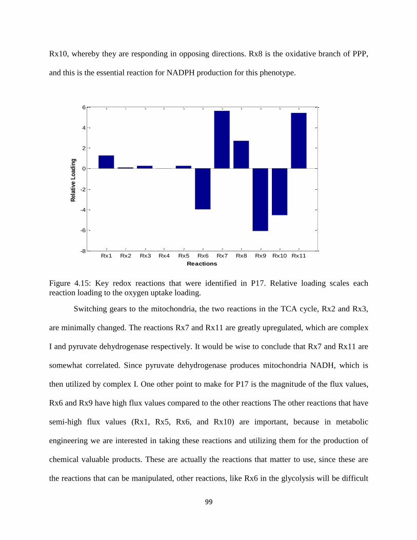
99

Rx10, whereby they are responding in opposing directions. Rx8 is the oxidative branch of PPP,

and this is the essential reaction for NADPH production for this phenotype.

Figure 4.15: Key redox reactions that were identified in P17. Relative loading scales each

reaction loading to the oxygen uptake loading.

Switching gears to the mitochondria, the two reactions in the TCA cycle, Rx2 and Rx3,

are minimally changed. The reactions Rx7 and Rx11 are greatly upregulated, which are complex

I and pyruvate dehydrogenase respectively. It would be wise to conclude that Rx7 and Rx11 are

somewhat correlated. Since pyruvate dehydrogenase produces mitochondria NADH, which is

then utilized by complex I. One other point to make for P17 is the magnitude of the flux values,

Rx6 and Rx9 have high flux values compared to the other reactions The other reactions that have

semi-high flux values (Rx1, Rx5, Rx6, and Rx10) are important, because in metabolic

engineering we are interested in taking these reactions and utilizing them for the production of

chemical valuable products. These are actually the reactions that matter to use, since these are

the reactions that can be manipulated, other reactions, like Rx6 in the glycolysis will be difficult

Rx1 Rx2 Rx3 Rx4 Rx5 Rx6 Rx7 Rx8 Rx9 Rx10 Rx11-8

-6

-4

-2

0

2

4

6

Reactions

Rel

ativ

e L

oad

ing

100

to perturb since this would mean that the glycolysis pathway would have to be affected, which

has many regulation schemes.

Table 4.8 Key redox reactions identified by SID framework for P17. Fluxs is the starting flux

value. Fluxe is the ending flux value. Flux ∆ is the difference between the Fluxs and Fluxe. The

units for the flux is mmol/gDW·hr. The Reaction # is the same reaction shown in Figure 4.15.

Reaction

#

Reaction Fluxs Fluxe Flux ∆

Rx1 h[c] + nadh[c] + akg[c] + nh4[c] <=> h2o[c] + nad[c] + glu-L[c] 0.39 0.40 0.01

Rx2 nad[m] + mal-L[m] <=> oaa[m] + h[m] + nadh[m] 0.033 0.035 0.002

Rx3 adp[m] + icit[m] -> akg[m] + nadph[m] + co2[m] 0.083 0.087 0.004

Rx4 h[c] + nadh[c] + dhap[c] -> nad[c] + glyc3p[c] 0.0023 0.0025 0.0002

Rx5 nad[c] + 3pg[c] -> h[c] + nadh[c] + 3php[c] 0.074 0.078 0.004

Rx6 nad[c] + pi[c] + g3p[c] <=> h[c] + nadh[c] + 13dpg[c] 7.4 7.3 -0.1

Rx7 5 h[m] + nadh[m] + q6[m] -> 4 h[c] + nad[m] + q6h2[m] 0.10 0.18 0.08

Rx8 nadp[c] + 6pgc[c] -> nadph[c] + co2[c] + ru5p-D[c] 0.02 0.06 0.04

Rx9 h[c] + acald[c] + nadh[c] <=> etoh[c] + nad[c] 6.80 6.70 -0.1

Rx10 nadp[c] + acald[c] + h2o[c] -> 2 h[c] + nadph[c] + ac[c] 0.22 0.15 -0.07

Rx11 coa[m] + pyr[m] + nad[m] -> accoa[m] + nadh[m] + co2[m] 0.048 0.13 0.082

For P16, surprisingly all the redox reactions are upregulated. Like P17, Rx6 and Rx9 are

heavily affected, but now they have reversed their direction. Rx4 had a very insignificant

response in P17, but in P16 it is highly upregulated. Rx1 remains quite similar as in P17. The

disturbance on the NADPH producing reactions are reduced, and so are complex I and pyruvate

dehydrogenase. It is important to point out that this phenotype is where ethanol production is

being increased. Could we use the behavior of this phenotype to discover ways to increase the

production of ethanol? It is difficult to give a clear answer to this question, but we do know what

is happening metabolically when ethanol production is increased. The results for P16 are shown

in Figure 4.16 for the loadings, and metabolic fluxes in Table 4.9.

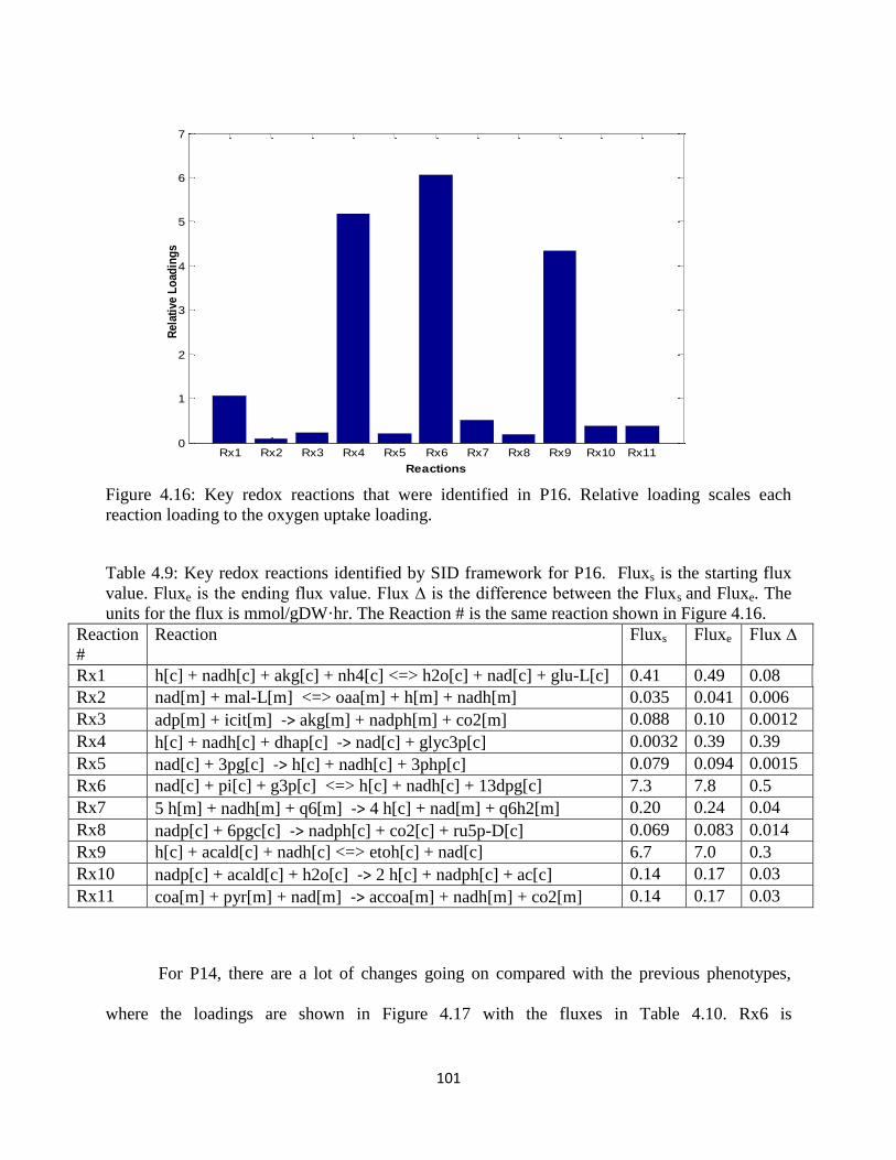
101

Figure 4.16: Key redox reactions that were identified in P16. Relative loading scales each

reaction loading to the oxygen uptake loading.

Table 4.9: Key redox reactions identified by SID framework for P16. Fluxs is the starting flux

value. Fluxe is the ending flux value. Flux ∆ is the difference between the Fluxs and Fluxe. The

units for the flux is mmol/gDW·hr. The Reaction # is the same reaction shown in Figure 4.16.

Reaction

#

Reaction Fluxs Fluxe Flux ∆

Rx1 h[c] + nadh[c] + akg[c] + nh4[c] <=> h2o[c] + nad[c] + glu-L[c] 0.41 0.49 0.08

Rx2 nad[m] + mal-L[m] <=> oaa[m] + h[m] + nadh[m] 0.035 0.041 0.006

Rx3 adp[m] + icit[m] -> akg[m] + nadph[m] + co2[m] 0.088 0.10 0.0012

Rx4 h[c] + nadh[c] + dhap[c] -> nad[c] + glyc3p[c] 0.0032 0.39 0.39

Rx5 nad[c] + 3pg[c] -> h[c] + nadh[c] + 3php[c] 0.079 0.094 0.0015

Rx6 nad[c] + pi[c] + g3p[c] <=> h[c] + nadh[c] + 13dpg[c] 7.3 7.8 0.5

Rx7 5 h[m] + nadh[m] + q6[m] -> 4 h[c] + nad[m] + q6h2[m] 0.20 0.24 0.04

Rx8 nadp[c] + 6pgc[c] -> nadph[c] + co2[c] + ru5p-D[c] 0.069 0.083 0.014

Rx9 h[c] + acald[c] + nadh[c] <=> etoh[c] + nad[c] 6.7 7.0 0.3

Rx10 nadp[c] + acald[c] + h2o[c] -> 2 h[c] + nadph[c] + ac[c] 0.14 0.17 0.03

Rx11 coa[m] + pyr[m] + nad[m] -> accoa[m] + nadh[m] + co2[m] 0.14 0.17 0.03

For P14, there are a lot of changes going on compared with the previous phenotypes,

where the loadings are shown in Figure 4.17 with the fluxes in Table 4.10. Rx6 is

Rx1 Rx2 Rx3 Rx4 Rx5 Rx6 Rx7 Rx8 Rx9 Rx10 Rx110

1

2

3

4

5

6

7

Reactions

Rela

tive L

oad

ing

s

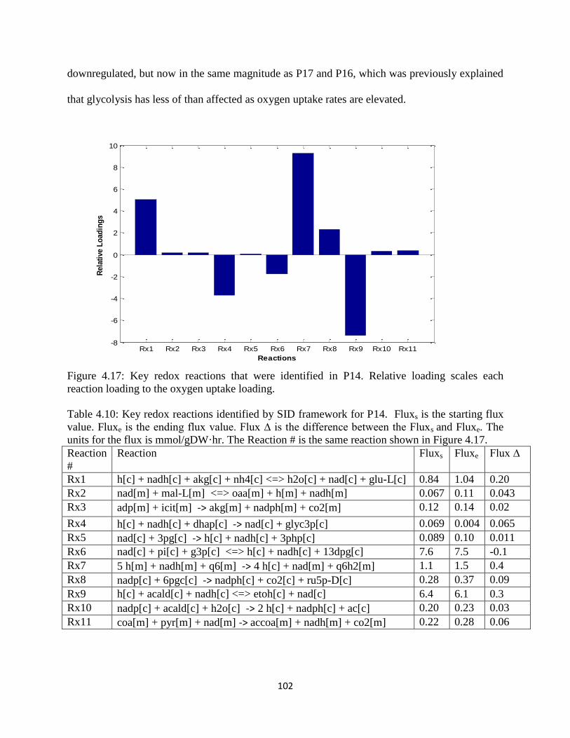
102

downregulated, but now in the same magnitude as P17 and P16, which was previously explained

that glycolysis has less of than affected as oxygen uptake rates are elevated.

Figure 4.17: Key redox reactions that were identified in P14. Relative loading scales each

reaction loading to the oxygen uptake loading.

Table 4.10: Key redox reactions identified by SID framework for P14. Fluxs is the starting flux

value. Fluxe is the ending flux value. Flux ∆ is the difference between the Fluxs and Fluxe. The

units for the flux is mmol/gDW·hr. The Reaction # is the same reaction shown in Figure 4.17.

Reaction

#

Reaction Fluxs Fluxe Flux ∆

Rx1 h[c] + nadh[c] + akg[c] + nh4[c] <=> h2o[c] + nad[c] + glu-L[c] 0.84 1.04 0.20

Rx2 nad[m] + mal-L[m] <=> oaa[m] + h[m] + nadh[m] 0.067 0.11 0.043

Rx3 adp[m] + icit[m] -> akg[m] + nadph[m] + co2[m] 0.12 0.14 0.02

Rx4 h[c] + nadh[c] + dhap[c] -> nad[c] + glyc3p[c] 0.069 0.004 0.065

Rx5 nad[c] + 3pg[c] -> h[c] + nadh[c] + 3php[c] 0.089 0.10 0.011

Rx6 nad[c] + pi[c] + g3p[c] <=> h[c] + nadh[c] + 13dpg[c] 7.6 7.5 -0.1

Rx7 5 h[m] + nadh[m] + q6[m] -> 4 h[c] + nad[m] + q6h2[m] 1.1 1.5 0.4

Rx8 nadp[c] + 6pgc[c] -> nadph[c] + co2[c] + ru5p-D[c] 0.28 0.37 0.09

Rx9 h[c] + acald[c] + nadh[c] <=> etoh[c] + nad[c] 6.4 6.1 0.3

Rx10 nadp[c] + acald[c] + h2o[c] -> 2 h[c] + nadph[c] + ac[c] 0.20 0.23 0.03

Rx11 coa[m] + pyr[m] + nad[m] -> accoa[m] + nadh[m] + co2[m] 0.22 0.28 0.06

Rx1 Rx2 Rx3 Rx4 Rx5 Rx6 Rx7 Rx8 Rx9 Rx10 Rx11-8

-6

-4

-2

0

2

4

6

8

10

Reactions

Rela

tive L

oad

ing

s

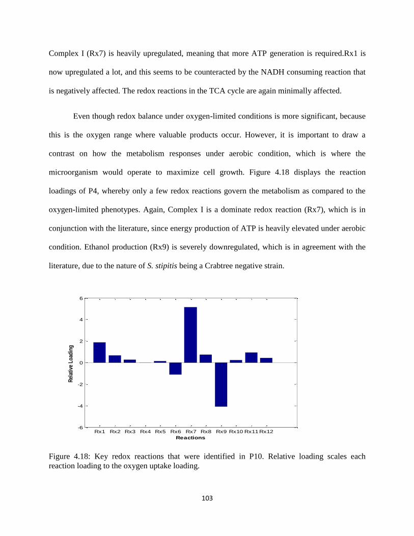
103

Complex I (Rx7) is heavily upregulated, meaning that more ATP generation is required.Rx1 is

now upregulated a lot, and this seems to be counteracted by the NADH consuming reaction that

is negatively affected. The redox reactions in the TCA cycle are again minimally affected.

Even though redox balance under oxygen-limited conditions is more significant, because

this is the oxygen range where valuable products occur. However, it is important to draw a

contrast on how the metabolism responses under aerobic condition, which is where the

microorganism would operate to maximize cell growth. Figure 4.18 displays the reaction

loadings of P4, whereby only a few redox reactions govern the metabolism as compared to the

oxygen-limited phenotypes. Again, Complex I is a dominate redox reaction (Rx7), which is in

conjunction with the literature, since energy production of ATP is heavily elevated under aerobic

condition. Ethanol production (Rx9) is severely downregulated, which is in agreement with the

literature, due to the nature of S. stipitis being a Crabtree negative strain.

Figure 4.18: Key redox reactions that were identified in P10. Relative loading scales each

reaction loading to the oxygen uptake loading.

Rx1 Rx2 Rx3 Rx4 Rx5 Rx6 Rx7 Rx8 Rx9 Rx10 Rx11Rx12-6

-4

-2

0

2

4

6

Reactions

Rel

ativ

e L

oad

ing

104

Rx1 continues to show up in all the phenotypes as the main NADH cytosolic consumption

reaction. The role of Rx5 on the metabolism was diminished greatly. The reaction loadings in the

TCA cycle increased, but it is still very small in comparison to Rx7 and Rx9. Table 4.11 shows

the flux values of the redox reactions. An extra reaction was added, which is in the TCA cycle,

this is the reaction that causes the TCA cycle to be unbranched.

Table 4.11: Key redox reactions identified by SID framework for P10. Fluxs is the starting flux

value. Fluxe is the ending flux value. Flux ∆ is the difference between the Fluxs and Fluxe. The

units for the flux is mmol/gDW·hr. The Reaction # is the same reaction shown in Figure 4.16.

Reaction

#

Reaction Fluxs Fluxe Flux ∆

Rx1 h[c] + nadh[c] + akg[c] + nh4[c] <=> h2o[c] + nad[c] + glu-

L[c]

1.4 2.3 0.9

Rx2 nad[m] + mal-L[m] <=> oaa[m] + h[m] + nadh[m] 0.18 0.54 0.36

Rx3 adp[m] + icit[m] -> akg[m] + nadph[m] + co2[m] 0.25 0.38 0.13

Rx4 h[c] + nadh[c] + dhap[c] -> nad[c] + glyc3p[c] 0.0047 0.0072 0.0025

Rx5 nad[c] + 3pg[c] -> h[c] + nadh[c] + 3php[c] 0.12 0.18 0.06

Rx6 nad[c] + pi[c] + g3p[c] <=> h[c] + nadh[c] + 13dpg[c] 7.4 6.8 -0.6

Rx7 5 h[m] + nadh[m] + q6[m] -> 4 h[c] + nad[m] + q6h2[m] 2.3 4.9 2.6

Rx8 nadp[c] + 6pgc[c] -> nadph[c] + co2[c] + ru5p-D[c] 0.47 0.82 0.35

Rx9 h[c] + acald[c] + nadh[c] <=> etoh[c] + nad[c] 5.4 3.4 -2.0

Rx10 nadp[c] + acald[c] + h2o[c] -> 2 h[c] + nadph[c] + ac[c] 0.23 0.35 0.12

Rx11 coa[m] + pyr[m] + nad[m] -> accoa[m] + nadh[m] + co2[m] 0.48 0.93 0.45

The finally phenotype that was examined was the line of optimality (LO), where Figure 4.19

convenes the redox reaction loadings, where the fluxes are accompanied in Table 4.12. The most

dominant redox reaction is Rx7, which tells us that the model favors this reaction pathway for

energy production. The next redox reaction that is responsible for governing the redox balance is

Rx6. It is not surprising that the electron transport chain and glycolysis pathway provides the

majority of variation of redox. Both of these are fundament pathways for carbon and energy

conversion. Other redox reactions that supply the redox variation is Rx1, Rx8, and Rx11.

105

Figure 4.19: Key redox reactions that were identified in LO. Relative loading scales each

reaction loading to the oxygen uptake loading.

Table 4.12: Key redox reactions identified by SID framework for LO. Fluxs is the starting flux

value. Fluxe is the ending flux value. Flux ∆ is the difference between the Fluxs and Fluxe. The

units for the flux is mmol/gDW·hr. The Reaction # is the same reaction shown in Figure 4.19.

Reaction

#

Reaction Fluxs Fluxe Flux ∆

Rx1 h[c] + nadh[c] + akg[c] + nh4[c] <=> h2o[c] + nad[c] + glu-

L[c]

0.33 2.0 1.67

Rx2 nad[m] + mal-L[m] <=> oaa[m] + h[m] + nadh[m] 0.40 2.7 2.3

Rx3 adp[m] + icit[m] -> akg[m] + nadph[m] + co2[m] 0.14 1.6 1.46

Rx4 h[c] + nadh[c] + dhap[c] -> nad[c] + glyc3p[c] 0.0026 0.0030 0.0004

Rx5 nad[c] + 3pg[c] -> h[c] + nadh[c] + 3php[c] 0.089 1.00 0.011

Rx6 nad[c] + pi[c] + g3p[c] <=> h[c] + nadh[c] + 13dpg[c] 1.1 10 8.9

Rx7 5 h[m] + nadh[m] + q6[m] -> 4 h[c] + nad[m] + q6h2[m] 3.1 25 21.9

Rx8 nadp[c] + 6pgc[c] -> nadph[c] + co2[c] + ru5p-D[c] 0.43 4.00 3.57

Rx9 h[c] + acald[c] + nadh[c] <=> etoh[c] + nad[c] 0 0 0

Rx10 nadp[c] + acald[c] + h2o[c] -> 2 h[c] + nadph[c] + ac[c] 0.13 1.4 1.27

Rx11 coa[m] + pyr[m] + nad[m] -> accoa[m] + nadh[m] + co2[m] 0.54 4.3 3.76

Rx1 Rx2 Rx3 Rx4 Rx5 Rx6 Rx7 Rx8 Rx9 Rx10 Rx11 Rx120

1

2

3

4

5

6

7

8

Reactions

Rel

ativ

e L

oad

ing

106

4.3.5 Limitations of iAD828

It is evident that iAD828 has made great strides in model performance, when examining

the SID framework and experimental validation results. Nonetheless, there are still limitations

that iAD828 imposes that if corrected would greatly strengthen the model prediction. Wet lab

experiments show that acetic acid is produced simultaneously with xylitol under oxygen-limited

conditions, where iAD828 lacks this capability (Kim, 2015). By using SID framework, the

phenotypes were analyzed and discovered that there were 20 phenotypes. The robustness under

low oxygen conditions is very poor; many phenotypes were generated with very small changes in

oxygen pickup rate. This error could be contributed to the lack of activation of alternative

oxidase, which is another route to reduce oxygen. Alternative oxidase has shown to be active

under very low oxygen levels (Shi et al., 2002), which could bring stability to the model. iAD828

chooses not activated alternative oxidase. Also under high oxygen conditions, there are

phenotypes appearing that have small differences in oxygen pickup rate.

4.4 Conclusion

A newly genome-scale metabolic model iAD828 of S. stipitis was developed through SID

framework, which supersedes the published models of iSS884 and iBB814. Validation done

through SID framework clearly demonstrates that key metabolic advances were accomplished in

iAD828: the xylose metabolism produced xylitol under oxygen-limited condition, both branches

of PPP are operating in the correct response for both oxygen-limited and aerobic condition, and

glycolysis is in the correct direction under oxygen-limited condition. Also the line of optimality

now exists for iAD828, which was incorrect for the previous models. The line of optimality can

provide great insight on what are the optimal metabolic conditions, and it has been shown to

quantitatively link the genotype with the phenotype through experiments (Edwards et al., 2002).

107

Other improvements were the correct metabolic behavior between the states of oxygen-limited

and aerobic condition, such as glycolysis fluxes higher under oxygen-limited condition, TCA

cycle fluxes higher under aerobic condition, and fatty acid biosynthesis higher under oxygen-

limited condition. The quantitative validation experiments favored iAD828 for two separate data

sets, and more importantly the qualitative validation experiment showed significant improvement

Also an additional experiment was compared with iAD828 in order to evaluated the in silico

predictions of xylitol production. These model improvements are essential to having a more

accurate depiction of the relationship between the genotype and phenotype. Here metabolic

information was extracted that expands our understanding of S. stipitis. This can provide

systematic assistance of the development of recombinant strains for the production of a

metabolite of interest.

108

Chapter 5: Cofactor engineering strategies for S. stipitis

5.1 Introduction

The regulation of catabolic and anabolic activity in microorganisms is essential for

determining the optimal phenotype for growth and producing biochemical valuable products

(Verho et al., 2003). The cofactors NAD(H) and NADP(H) play unique roles in the metabolism,

whereby NADH is primarily used in the catabolism, while NADPH prefers usage in the

anabolism. The respiratory cofactor NADH is principally utilized for ATP production through

transferring electrons to oxygen through electron transport chain. Cytosolic NADH is generated

from the sugar dissimilation subsystem of glycolysis, while the TCA cycle provides

mitochondria NADH. Concurrently, NADPH provides electrons for biosynthetic reactions, such

as amino acid synthesis. Production of cytosolic NADPH is accomplished in the oxidative

branch of PPP and pyruvate metabolism by the aldehyde dehydrogenase reaction. Despite the

different functions of NADH and NADPH, they are interconnected to each other, for example

glycolysis provides building blocks for anabolic reactions and central metabolites, while

pyruvate and acetyl-CoA are used as precursors for biosynthetic reactions (Heux et al., 2006;

Hou et al., 2009; Wandrey, 2004)

Under oxygen-limitations, NADH is in excess, and is re-oxidized for ethanol production.

Also the byproduct xylitol is produced, because of a cofactor imbalance of the first two reactions

(xylose reductase and xylitol dehydrogenase) of the xylose metabolism (Passoth et al., 1996).

Xylose reductase uses both NADH and NADPH, and xylitol dehydrogenase utilizes only NAD;

however some literature shows even NADP is used (Jeffries, 2006; Watanabe et al., 2007).

As demonstrated from the previous chapter, iAD828 provides significant performance

enhancement, therefore we want to use this model to guide metabolic engineering strategies for

109

overproduction of ethanol. The cofactor balance is an important element to solve, because there

is yet a concrete conclusion and it is a very significant issue for the S. cerevisiae recombinant

strain

5.2 Materials and methods

5.2.1 In silico experiments

The genome-scale metabolic model of iAD828 were evaluated by flux balance analysis

(FBA), in which the COBRA toolbox (Schellenberger et al., 2011) was used. The objective

function of growth was used for all in silico experiments, except for case study that switched the

objective function to ethanol production. For optimization of ethanol, growth was set at 80 % of

the optimal solution for growth (when the objective function is optimization of growth). The

upper limits of xylose and oxygen uptakes were varied based on the preselected conditions,

while the other exchange compounds (NH4+

, H+, SO4

2-, Pi

2-, H2O, Fe

2+) were given the option to

enter and exit the network freely, with upper and lower bounds of -1000 to 1000 mmol/gDW·hr.

The final metabolic products (CO2, ethanol, acetic acid, etc.) were allowed to exit the system

freely, where the reaction flux was constrained to 0 – 1000 mmol/gDW·hr, which prevents

product uptake. The growth associated maintenance energy was set to 2.6 mmol/gDW·hr

(Balagurunathan et al., 2012).

5.2.2 SID framework

As in the Chapter 4 and 5, SID framework was used to identify the essential reactions in

each phenotype. Different input variables were used to perturb the system, such as oxygen

pickup rate and xylose reductase redox ratio preference (NADPH/NADH). The results are then

visualized through metabolic colored maps.

110

5.3 Results and Discussion

Cofactor engineering of the xylose metabolism and the redox balance was investigated to

extract embedded metabolic information for the overproduction of ethanol. Xylose reductase

preference for NADPH and NADH was altered and SID framework was used to extract the

essential metabolic information. Conclusions from this data allowed for uncovering specific

strategies and they were imposed on iAD828 for overproduction of ethanol.

5.3.1 Background of cofactor engineering of xylose reductase

S. stipitis is only a handful of strains that have the native ability to digest xylose for

ethanol production; therefore genes from the xylose metabolism have been used to construct

recombinant strains, such as S. cerevisiae. The incorporation of the xylose metabolism into the

recombinant strain has shown to be inefficient due to have a cofactor imbalance for the first two

reactions in the xylose metabolism, xylose reductase (XR) and xylitol dehydrogenase (XDH)

(Jeppsson et al., 2002). Figure 5.1 displays the first three steps for the xylose metabolism in S.

stitipis, with the corresponding cofactor preference. Xylose reductase has shown to have a dual

preference for NADH and NADPH, while xylitol dehydrogenase has shown to predominantly

use NAD alone, however reports have shown NADP route is also feasible. In S. stitipis, the

xylose metabolism and the cofactor regeneration is poorly understood, thus gaining fundament

understanding will equip biologist with strategies to make improved recombinant strains.

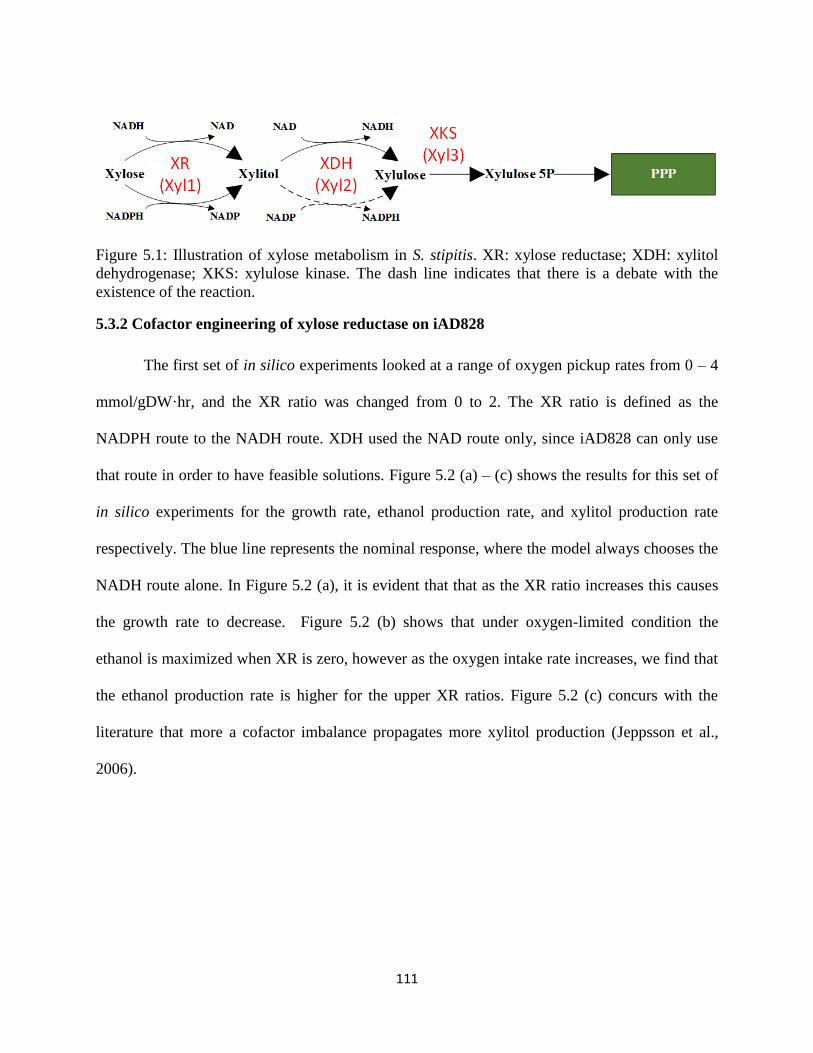
111

Figure 5.1: Illustration of xylose metabolism in S. stipitis. XR: xylose reductase; XDH: xylitol

dehydrogenase; XKS: xylulose kinase. The dash line indicates that there is a debate with the

existence of the reaction.

5.3.2 Cofactor engineering of xylose reductase on iAD828

The first set of in silico experiments looked at a range of oxygen pickup rates from 0 – 4

mmol/gDW·hr, and the XR ratio was changed from 0 to 2. The XR ratio is defined as the

NADPH route to the NADH route. XDH used the NAD route only, since iAD828 can only use

that route in order to have feasible solutions. Figure 5.2 (a) – (c) shows the results for this set of

in silico experiments for the growth rate, ethanol production rate, and xylitol production rate

respectively. The blue line represents the nominal response, where the model always chooses the

NADH route alone. In Figure 5.2 (a), it is evident that that as the XR ratio increases this causes

the growth rate to decrease. Figure 5.2 (b) shows that under oxygen-limited condition the

ethanol is maximized when XR is zero, however as the oxygen intake rate increases, we find that

the ethanol production rate is higher for the upper XR ratios. Figure 5.2 (c) concurs with the

literature that more a cofactor imbalance propagates more xylitol production (Jeppsson et al.,

2006).

112

Figure 5.2: Cofactor XR ratio influence on iAD828. (a) growth rate, (b) ethanol production rate,

and (c) xylitol production rate

0 0.5 1 1.5 2 2.5 3 3.5 40

0.05

0.1

0.15

0.2

0.25

0.3

0.35

(a)

Oxygen uptake rate (mmol/gDW/hr)

Gro

wth

ra

te (

hr-1

)

NADPH/NADH=0

NADPH/NADH=0.4

NADPH/NADH=0.8

NADPH/NADH=1.2

NADPH/NADH=1.6

NADPH/NADH=2

0 0.5 1 1.5 2 2.5 3 3.5 40

1

2

3

4

5

6

7

8

9

(b)

Oxygen uptake rate (mmol/gDW/hr)

Eth

an

ol (m

mo

l/g

DW

/hr)

NADPH/NADH=0

NADPH/NADH=0.4

NADPH/NADH=0.8

NADPH/NADH=1.2

NADPH/NADH=1.6

NADPH/NADH=2

0 1 2 3 40

0.5

1

1.5

2

2.5

3

3.5

(e)

Oxygen uptake rate (mmol/gDW/hr)

Xyl

itol (

mm

ol/g

DW

/hr)

NADPH/NADH=0

NADPH/NADH=0.4

NADPH/NADH=0.8

NADPH/NADH=1.2

NADPH/NADH=1.6

NADPH/NADH=2

a

b

c

113

Further investigation was conducted that examined if there was consistency between the

phenotypes in the regions of maximum ethanol production under oxygen-limited condition and

higher oxygen pickup levels. Except for the XR ratio at zero, all the rest of the XR ratios at the

maximum ethanol production rate belonged to the same phenotype. Since the highest ethanol

production rate occurs under oxygen-limited condition, in silico experiments were then

conducted under this condition. The oxygen pickup ranged from 0 to 1 mmol/gDW·hr and the

XR ratio was varied now from 0 to 0.4, since this is the ratio that belong to optimal ethanol

production. Figure 5.3 exhibits the ethanol production rate for this in silico experiment, where

there are two ethanol production regions, which represent two different phenotypes, P17 and

P16. P17 phenotypic space is represented by a solid black line, which means solutions along this

line belong to P17, likewise the same is true for P16 as it is represented as the dash black line.

Recalling back to Chapter 4 to the 2D phenotype phase plane plots in Figure 4.6, P17

only inhabits a very small region, while P16 is much wider. It would be very difficult to keep wet

lab experiments in P17, thus P16 is better option to run wet lab experiments. Further examination

was performed on P16, where fluxes where collected along the P16 line as XR ratio increased

and SID framework was then applied to extract the embedded metabolic information. Table 5.1

shows the results of the flux values of the starting and ending points, and the loadings. For this

analysis it is important to taken into consideration both the flux and loading, since just because

there is a high loading value does not mean that it has a great impact on the system.

114

Figure 5.3: Influence of cofactor preference of XR ratio under oxygen-limited condition. P17 is

represented by solid black line. P16 is represented by a dash black line.

Table 5.1: Reactions influenced by variation of XR ratio for P16. Fluxs is the starting flux value

and Fluxe is the ending flux value. The loading taken from SID framework, which is normalized

to the XR ratio

Reaction

#

Reaction Fluxs Fluxe Loading

Rx1 h[c] + nadh[c] + akg[c] + nh4[c] -> h2o[c] + nad[c] + glu-L[c] 0.49 0.33 -0.11

Rx2 h[c] + nadh[c] + dhap[c] -> nad[c] + glyc3p[c] 0.40 0.52 0.088

Rx3 h[c] + acald[c] + nadh[c] -> etoh[c] + nad[c] 7.0 5.3 -1.2

Rx4 nad[c] + pi[c] + g3p[c] -> h[c] + nadh[c] + 13dpg[c] 7.8 5.8 -1.4

Rx5 nad[c] + xylt[c] -> nadh[c] + xylu-D[c] + h[c] 5 3.8 -0.82

Rx6 5 h[m] + nadh[m] + q6[m] -> 4 h[c] + nad[m] + q6h2[m] 0.24 0.16 -0.054

Rx7 coa[m] + pyr[m] + nad[m] -> accoa[m] + nadh[m] + co2[m] 0.17 0.11 -0.04

Rx8 nadp[c] + 6pgc[c] -> nadph[c] + co2[c] + ru5p-D[c] 0.083 0.77 0.48

Rx9 nadp[c] + acald[c] + h2o[c] -> 2 h[c] + nadph[c] + ac[c] 0.17 0.12 -0.04

Rx10 nadp[m] + icit[m] -> akg[m] + nadph[m] + co2[m] 0.11 0.071 -0.024

Rx11 8 h[m] + o2[m] + 4 focytc[m] -> 4 h[c] + 2 h2o[m] + 4

ficytc[m]

0.32 0.34 0.017

Rx12 xu5p-D[c] -> ru5p-D[c] 1.6 0.78 - 0.60

Rx13 r5p[c] + xu5p-D[c] <=> g3p[c] + s7p[c] 1.7 1.5 -0.11

Rx14 h[c] + pyr[c] -> acald[c] + co2[c] 7.2 5.4 -1.3

Rx15 atp[c] + xylu-D[c] --> h[c] + adp[c] + xu5p-D[c] 5.0 3.8 -0.82

0 0.1 0.2 0.3 0.4 0.5 0.6 0.7 0.8 0.9 14

4.5

5

5.5

6

6.5

7

7.5

8

(b)

Oxygen uptake rate (mmol/gDW/hr)

Eth

an

ol (m

mo

l/g

DW

/hr)

NADPH/NADH=0

NADPH/NADH=0.1

NADPH/NADH=0.2

NADPH/NADH=0.3

NADPH/NADH=0.4

P17 P16

115

5.3.3 Potential metabolic engineering strategies

Oxidative branch of PPP is the leading producer of NADPH, and is heavily affected in

the opposite direction of ethanol production, thus more NADPH production from the oxidative

PPP results in decrease ethanol production. Some metabolic engineering strategies to consider

are having another NADPH producing reaction to be the principal reaction for NADPH

generation (Bro et al., 2006). This could be done by redirection of the flux away from the

oxidative branch of PPP to the pyruvate metabolism via aldehyde dehydrogenase, Rx9. The

indication of redirection of the flux away from the oxidative branch of PPP can also be supported

by Rx12 and Rx13, where upregulation of these reactions is would propagate away from a

decrease in ethanol production. A strategy that has been implored in S. cerevisiae is inserting

NADP+-dependent D-glyceraldehyde-3-phosphate dehydrogenase and blocking the oxidative

branch of PPP. The reaction that is being added is part of the glycolysis pathway, where there

exists a NAD+-dependent D-glyceraldehyde-3-phosphate dehydrogenase reaction, Rx4

(Matsushika et al., 2009a). Based on the results, Rx4 has a negative correlation to ethanol

decrease; therefore having more flux through this reaction would improve ethanol production.

Another thought is that the oxidative branch of PPP is considered an anabolic pathway, because

of the involvement of NADPH production that is used for generation of building blocks for

biomass formation, thus pushing fluxes toward catabolic pathways would be more profitable for

ethanol production. For NADH consumption reactions, which are Rx1 and Rx2, more benefit for

maximizing ethanol production would be to upregulate Rx1 and downregulate Rx2. Moving to

the electron transport chain, complex IV downregulation shows that it would increase ethanol

production, and the opposite is true for complex I that upregulation would increase ethanol

production. However, for complex I and complex IV the loading value is not significantly

116

affected. Rx15, known as xylulokinase (XKS), upregulating this would provide for ethanol

production rate incresase.

5.3.4 Switching the objective function to ethanol production rate

Another consideration is changing the objective function from biomass formation to

ethanol production. In order to prevent zero biomass growth, the biomass was held at 80 % of the

nominal value for this condition. The intent of this was to see if any clear occurrence of

upregulation or deregulation of reaction pathways existed. This could provide additional

information that could be used for metabolic engineering strategies. As the previous analysis, the

oxidative branch of PPP was again recognized as an important element for manipulation of

ethanol production. Also the glycolysis pathway and Rx1 again showed to by parts of the

metabolism deemed to be vital.

5.3.5 Metabolic engineering strategy 1

The first metabolic engineering strategy that was proposed was deletion of glucose 6-

phosphate dehydrogenase, which would completely inhibit the oxidative branch of PPP, inserting

of NADP+-dependent D-glyceraldehyde-3-phosphate dehydrogenase, and deletion of NAD+-

dependent D-glyceraldehyde-3-phosphate dehydrogenase. The justification of this strategy is

taken from the fact that upregulation of the oxidative branch of PPP seems to be detrimental for

ethanol production. The NADP+-dependent D-glyceraldehyde-3-phosphate dehydrogenase

provides for an alternative way to produce NADPH, and more flux would be redirected to the

pyruvate metabolism for ethanol production. Figure 5.4 (a) – (c) displays the results of iAD828

and iAD828-ME1 (metabolic engineering strategy 1) and how it influenced growth rate, ethanol,

and xylitol respectively.

117

Figure 5.4. Metabolic engineering strategy 1. (a) growth rate, (b) ethanol, (c) xylitol. The red

line is iAD828 and the blue line contains the metabolic engineering strategy 1 (iAD828-ME1)

0 0.1 0.2 0.3 0.4 0.5 0.6 0.7 0.8 0.9 10

0.02

0.04

0.06

0.08

0.1

0.12

0.14

Oxygen uptake (mmol/gDW*hr)

Gro

wth

ra

te (

mm

ol/g

DW

*hr)

iAD828

iAD828-ME1

0 0.1 0.2 0.3 0.4 0.5 0.6 0.7 0.8 0.9 1

6

6.2

6.4

6.6

6.8

7

7.2

7.4

7.6

7.8

Oxygen uptake (mmol/gDW*hr)

Eth

an

ol (m

mo

l/g

DW

*hr)

iAD828

iAD828-ME1

0 0.1 0.2 0.3 0.4 0.5 0.6 0.7 0.8 0.9 10

0.1

0.2

0.3

0.4

0.5

0.6

0.7

0.8

0.9

Oxygen uptake (mmol/gDW*hr)

Xy

lito

l (m

mo

l/g

DW

*hr)

iAD828

iAD828-ME1

b

a

c

118

Figure 5.4 (a) shows that the growth rate is higher for iAD828-ME1 than iAD828, which is due

having less carbon by converted into CO2 via the oxidative PPP. Figure 5.4 (b) shows that the

ethanol production is higher for iAD828-ME1 (excluding the first point of iAD828) for oxygen

pickup rates less than 0.35 mmol/gDW·hr. For the highest ethanol production rate points in both

models, iAD828-ME1 has a perecent increase of 7.8 % than iAD828. In the mid region of the

Figure 5.4 (b), iAD828 has higher ethanol production. Figure 5.4 (c) shows that iAD828-ME1

was able to eliminate xylitol production. Further analysis was done in the region of optimal

ethanol production through SID framework, for the oxygen pickup range of 0.03 – 0.14

mmol/gDW·hr. SID framework revealed that Rx1 was heavily downregulated. Other findings

were that the non-oxidative branch of PPP was downregulated. Also glycolysis was split into two

regions, the upper part was downregulation (until glyceraldehyde 3 phosphate production) and

the lower part was upregulated.

5.3.6 Metabolic engineering strategy 2

From this analysis, another strategy was proposed, iAD828-ME2, which kept the same

setup as metabolic engineering 1, except that Rx1 was deleted. The intuition behind this was that

Rx1 was a main consumer of NADH, which when deleted would provide more NADH for

ethanol production. Figure 5.5 (a) and (b) shows how the growth rate and ethanol production rate

was influenced respectively for this strategy compared with iAD828 and iAD828-ME1. The

growth rate is the lowest for iAD828-ME2, which is shown by the green line; therefore deletion

of Rx1 is directly correlated to growth rate. This is due to Rx1 being a glutamate production

reaction, and with deletion of Rx1 this causes the model to select another reaction for glutamate

production, which the precursor reaction requires ATP consumption. With the decrease in carbon

119

flux flowing to cellular growth this allows for carbon to be directed to ethanol production, which

results in iAD828-ME2 having the highest ethanol production rate.

0 0.1 0.2 0.3 0.4 0.5 0.6 0.7 0.8 0.9 1

6

6.2

6.4

6.6

6.8

7

7.2

7.4

7.6

7.8

Oxygen uptake (mmol/gDW*hr)

Eth

an

ol (m

mo

l/g

DW

*hr)

iAD828

iAD828-ME1

iAD828-ME2

0 0.1 0.2 0.3 0.4 0.5 0.6 0.7 0.8 0.9 10

0.02

0.04

0.06

0.08

0.1

0.12

0.14

Oxygen uptake (mmol/gDW*hr)

Gro

wth

ra

te (

mm

ol/g

DW

*hr)

iAD828

iAD828-ME1

iAD828-ME2

Figure 5.5. Metabolic engineering strategy 2. (a) Growth rate and (b) ethanol.The red line is

iAD828, the blue line contains the metabolic engineering strategy 1 (iAD828-ME1), and the

green line represents metabolic engineering strategy 2 (iAD828-ME2)

a

b

120

5.4 Conclusion

Due to the metabolic advancements of iAD828, cofactor engineering strategies was

applied in order to delegate carbon flux toward ethanol overproduction. Great exposure has been

toward the first two steps in the xylose metabolism: xylose reductase and xylitol dehydrogenase,

since these enzymes have been inserted into S. cerevisiae in order to make a recombinant strain

for ethanol overproduction, and have shown to be responsible for the cofactor imbalance. This

propagated in silico experiments that varied the xylose reductase ratio (NADPH/NADH).

iAD828 adheres to the literature, where ethanol production is highest and xylitol production is

the lowest when the xylose reductase ratio is the lowest. P16 is the phenotype responsible for

optimal ethanol production conditions and SID framework was used to analyze the phenotype.

The oxidative branch of PPP was shown to be highly involved in ethanol production, and it

would be more favorable if the carbon flux was redirect to the pyruvate metabolism. Based on

these results, metabolic engineering strategies were instilled and ethanol overproduction was

accomplished.

121

Chapter 6: A System Identification Based Approach for Phenotype Phase

Plane Analysis

6.1 Introduction

The arrival of genome sequencing has brought about the reconstruction of genome-scale

models, which provide a systems level understanding of a cellular metabolism through in silico

methods (Kim et al., 2012). The constraint-based methods have been used on metabolic networks

for more than 25 years (Lewis et al., 2012). Metabolic phenotypes of microorganisms are

elucidated from these methods that are based on the environmental conditions and the genotype

(Karr et al., 2012). One prevalent constraint-based method, phenotype phase plane (PhPP)

analysis, provides a global view of each phenotype in genome-scale models by breaking down

the metabolic behavior in distinct phases through shadow prices analysis. The shadow price is

defined as the effect of the metabolite concentration on the objective function. Two independent

variables, typically the carbon and oxygen source, are varied, and the shadow price is calculated

for each metabolite. Shadow price analysis has the capability to find if metabolites are limited or

in excess, and if metabolites are expelled from the network. The cellular growth is mapped on a

two-dimensional plane, which is calculated by varying the two independent variables. The

phases describe the metabolic phenotypes, and each phase denotes that the shadow prices of each

metabolite are constant (Edwards et al., 2012).

Metabolic phenotypes can be thought of different utilization profiles, in other words each

phenotype has a unique flux distribution (Varma et al., 1994). Figure 6.1 demonstrates this idea,

where PhPP analysis was performed on the genome-scale model of iAD828. The two

independent variables are are xylose and oxygen. Each phenotype is characterized by a different

color, for example in Figure 6.1, the yellow region and green region represent separate

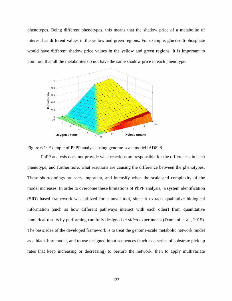
122

phenotypes. Being different phenotypes, this means that the shadow price of a metabolite of

interest has different values in the yellow and green regions. For example, glucose 6-phosphate

would have different shadow price values in the yellow and green regions. It is important to

point out that all the metabolites do not have the same shadow price in each phenotype.

Figure 6.1: Example of PhPP analysis using genome-scale model iAD828.

PhPP analysis does not provide what reactions are responsible for the differences in each

phenotype, and furthermore, what reactions are causing the difference between the phenotypes.

These shortcomings are very important, and intensify when the scale and complexity of the

model increases. In order to overcome these limitations of PhPP analysis, a system identification

(SID) based framework was utilized for a novel tool, since it extracts qualitative biological

information (such as how different pathways interact with each other) from quantitative

numerical results by performing carefully designed in silico experiments (Damiani et al., 2015).

The basic idea of the developed framework is to treat the genome-scale metabolic network model

as a black-box model, and to use designed input sequences (such as a series of substrate pick up

rates that keep increasing or decreasing) to perturb the network; then to apply multivariate

02

46

810

0

2

4

6

8

100

0.2

0.4

0.6

0.8

1

Xylose uptake Oxygen uptake

Gro

wth

ra

te

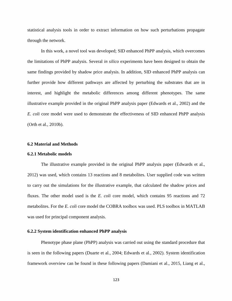
123

statistical analysis tools in order to extract information on how such perturbations propagate

through the network.

In this work, a novel tool was developed; SID enhanced PhPP analysis, which overcomes

the limitations of PhPP analysis. Several in silico experiments have been designed to obtain the

same findings provided by shadow price analysis. In addition, SID enhanced PhPP analysis can

further provide how different pathways are affected by perturbing the substrates that are in

interest, and highlight the metabolic differences among different phenotypes. The same

illustrative example provided in the original PhPP analysis paper (Edwards et al., 2002) and the

E. coli core model were used to demonstrate the effectiveness of SID enhanced PhPP analysis

(Orth et al., 2010b).

6.2 Material and Methods

6.2.1 Metabolic models

The illustrative example provided in the original PhPP analysis paper (Edwards et al.,

2012) was used, which contains 13 reactions and 8 metabolites. User supplied code was written

to carry out the simulations for the illustrative example, that calculated the shadow prices and

fluxes. The other model used is the E. coli core model, which contains 95 reactions and 72

metabolites. For the E. coli core model the COBRA toolbox was used. PLS toolbox in MATLAB

was used for principal component analysis.

6.2.2 System identification enhanced PhPP analysis

Phenotype phase plane (PhPP) analysis was carried out using the standard procedure that

is seen in the following papers (Duarte et al., 2004; Edwards et al., 2002). System identification

framework overview can be found in these following papers (Damiani et al., 2015, Liang et al.,

124

2013). The SID enhanced PhPP analysis visualized in the block diagram is shown in Figure 6.2.

The first block is selection of a particular metabolite to vary; in this case, an input to the system,

like carbon or oxygen. By perturbing the system with the input flux, the fluxes of all the

reactions are recorded, and then principal component analysis (PCA) is performed. The

justification of why PCA is used is that the flux matrix as a multivariable problem, where the

variables are the specific reactions and the system is sampled by varying the substrate uptake

rate. PCA reduces the dimensionality of the flux matrix to uncorrelated components, known as

principal components, which is the linear combination of the original variables. In all our cases

one principal component was used to describe all the variation. From PCA, two outputs are

given, known as scores and loadings. The scores represent a composite measurement for each

sample that is taken; therefore provide a global measurement of what is going on in the model

network. Thus the scores provide the number of phenotypes by examining the linear behavior of

each score value. When the flux profile changes this causes a different linear segment, which

designates a new phenotype. On the other hand, the loadings are weightings for each variable,

which tell us how important each reaction is. Whether a reaction is active or non-active, and if

being active, whether is it being upregulated or downregulated, and the corresponding weighting.

Comparing SID enhanced PhPP analysis to PhPP analysis, this now allows the different

phenotypes to be determined by the scores rather than the shadow prices. This is advantageous,

because the whole phenotype plane does not need to be calculated at every carbon and oxygen

point, but rather that the boundaries are calculated through the SID enhanced PhPP analysis.

Also the accuracy of where each phase exists, it not affected by the grid size, as the PhPP

analysis was.

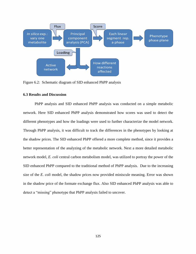
125

Figure 6.2: Schematic diagram of SID enhanced PhPP analysis

6.3 Results and Discussion

PhPP analysis and SID enhanced PhPP analysis was conducted on a simple metabolic

network. Here SID enhanced PhPP analysis demonstrated how scores was used to detect the

different phenotypes and how the loadings were used to further characterize the model network.

Through PhPP analysis, it was difficult to track the differences in the phenotypes by looking at

the shadow prices. The SID enhanced PhPP offered a more complete method, since it provides a

better representation of the analyzing of the metabolic network. Next a more detailed metabolic

network model, E. coli central carbon metabolism model, was utilized to portray the power of the

SID enhanced PhPP compared to the traditional method of PhPP analysis. Due to the increasing

size of the E. coli model, the shadow prices now provided miniscule meaning. Error was shown

in the shadow price of the formate exchange flux. Also SID enhanced PhPP analysis was able to

detect a “missing” phenotype that PhPP analysis failed to uncover.

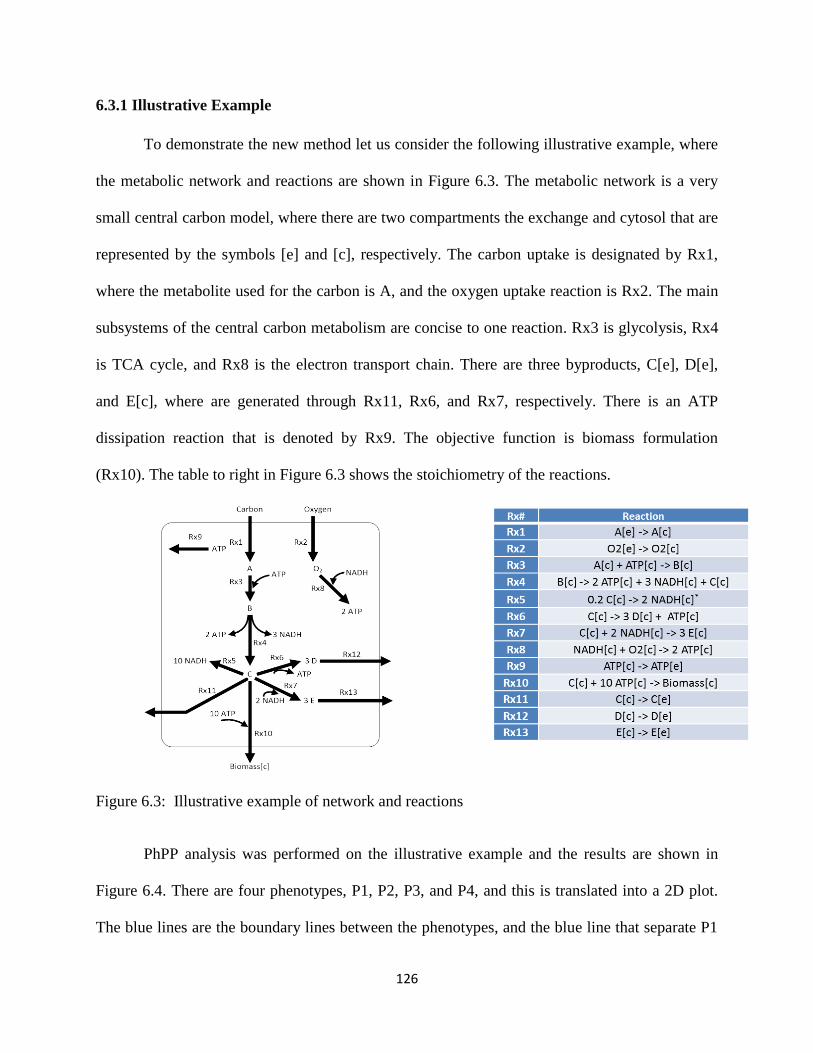
126

6.3.1 Illustrative Example

To demonstrate the new method let us consider the following illustrative example, where

the metabolic network and reactions are shown in Figure 6.3. The metabolic network is a very

small central carbon model, where there are two compartments the exchange and cytosol that are

represented by the symbols [e] and [c], respectively. The carbon uptake is designated by Rx1,

where the metabolite used for the carbon is A, and the oxygen uptake reaction is Rx2. The main

subsystems of the central carbon metabolism are concise to one reaction. Rx3 is glycolysis, Rx4

is TCA cycle, and Rx8 is the electron transport chain. There are three byproducts, C[e], D[e],

and E[c], where are generated through Rx11, Rx6, and Rx7, respectively. There is an ATP

dissipation reaction that is denoted by Rx9. The objective function is biomass formulation

(Rx10). The table to right in Figure 6.3 shows the stoichiometry of the reactions.

Figure 6.3: Illustrative example of network and reactions

PhPP analysis was performed on the illustrative example and the results are shown in

Figure 6.4. There are four phenotypes, P1, P2, P3, and P4, and this is translated into a 2D plot.

The blue lines are the boundary lines between the phenotypes, and the blue line that separate P1

127

and P2 is known as the line of optimality (LO), which is defined as the optimal ratio of oxygen

and carbon uptake. The green regions in the 3D plot represent the infeasible regions, which are

shown in the 2D plot by the light blue regions.

Figure 6.4: PhPP analysis of illustrative example

The SID enhanced PhPP analysis calculates the scores by varying one independent

variable at a time, where this can be done for each variable. The results of this analysis are

shown in Figure 6.5. The scores calculated when varying the carbon flux are shown by the plot at

the bottom left corner. While the plot to the right shows the scores plot for varying oxygen flux.

The linearity of each line segment represents a specific phenotype, and the direction of the linear

segment changes represents shifting into another phenotype. For example, the boundary line

between P2 and P3 shows that the scores plot of oxygen and carbon is determined at different

points on the boundary line, thus the two points are connected and the boundary line is found.

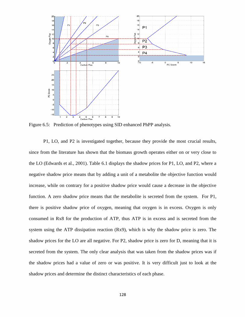
128

Figure 6.5: Prediction of phenotypes using SID enhanced PhPP analysis.

P1, LO, and P2 is investigated together, because they provide the most crucial results,

since from the literature has shown that the biomass growth operates either on or very close to

the LO (Edwards et al., 2001). Table 6.1 displays the shadow prices for P1, LO, and P2, where a

negative shadow price means that by adding a unit of a metabolite the objective function would

increase, while on contrary for a positive shadow price would cause a decrease in the objective

function. A zero shadow price means that the metabolite is secreted from the system. For P1,

there is positive shadow price of oxygen, meaning that oxygen is in excess. Oxygen is only

consumed in Rx8 for the production of ATP, thus ATP is in excess and is secreted from the

system using the ATP dissipation reaction (Rx9), which is why the shadow price is zero. The

shadow prices for the LO are all negative. For P2, shadow price is zero for D, meaning that it is

secreted from the system. The only clear analysis that was taken from the shadow prices was if

the shadow prices had a value of zero or was positive. It is very difficult just to look at the

shadow prices and determine the distinct characteristics of each phase.

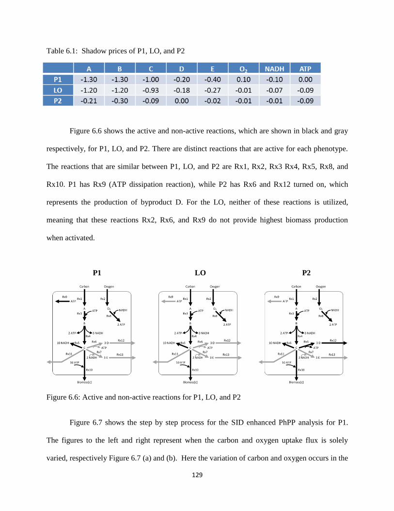
129

Table 6.1: Shadow prices of P1, LO, and P2

Figure 6.6 shows the active and non-active reactions, which are shown in black and gray

respectively, for P1, LO, and P2. There are distinct reactions that are active for each phenotype.

The reactions that are similar between P1, LO, and P2 are Rx1, Rx2, Rx3 Rx4, Rx5, Rx8, and

Rx10. P1 has Rx9 (ATP dissipation reaction), while P2 has Rx6 and Rx12 turned on, which

represents the production of byproduct D. For the LO, neither of these reactions is utilized,

meaning that these reactions Rx2, Rx6, and Rx9 do not provide highest biomass production

when activated.

Figure 6.6: Active and non-active reactions for P1, LO, and P2

Figure 6.7 shows the step by step process for the SID enhanced PhPP analysis for P1.

The figures to the left and right represent when the carbon and oxygen uptake flux is solely

varied, respectively Figure 6.7 (a) and (b). Here the variation of carbon and oxygen occurs in the

P1 LO P2

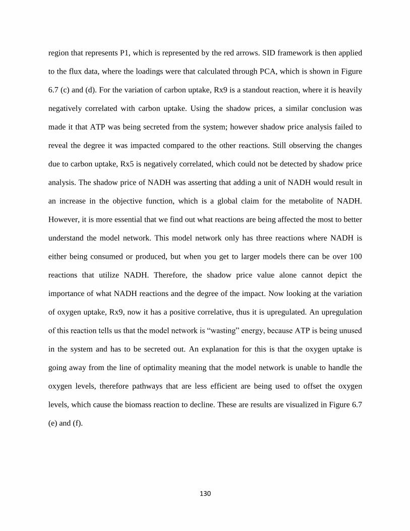
130

region that represents P1, which is represented by the red arrows. SID framework is then applied

to the flux data, where the loadings were that calculated through PCA, which is shown in Figure

6.7 (c) and (d). For the variation of carbon uptake, Rx9 is a standout reaction, where it is heavily

negatively correlated with carbon uptake. Using the shadow prices, a similar conclusion was

made it that ATP was being secreted from the system; however shadow price analysis failed to

reveal the degree it was impacted compared to the other reactions. Still observing the changes

due to carbon uptake, Rx5 is negatively correlated, which could not be detected by shadow price

analysis. The shadow price of NADH was asserting that adding a unit of NADH would result in

an increase in the objective function, which is a global claim for the metabolite of NADH.

However, it is more essential that we find out what reactions are being affected the most to better

understand the model network. This model network only has three reactions where NADH is

either being consumed or produced, but when you get to larger models there can be over 100

reactions that utilize NADH. Therefore, the shadow price value alone cannot depict the

importance of what NADH reactions and the degree of the impact. Now looking at the variation

of oxygen uptake, Rx9, now it has a positive correlative, thus it is upregulated. An upregulation

of this reaction tells us that the model network is “wasting” energy, because ATP is being unused

in the system and has to be secreted out. An explanation for this is that the oxygen uptake is

going away from the line of optimality meaning that the model network is unable to handle the

oxygen levels, therefore pathways that are less efficient are being used to offset the oxygen

levels, which cause the biomass reaction to decline. These are results are visualized in Figure 6.7

(e) and (f).

131

Figure 6.7: SID enhanced PhPP analysis for P1. (a) Variation of carbon in 2D phenotype plot,

(b) Variation of oxygen in 2D phenotype plot, (c) Loadings for variation of carbon, (d) Loadings

for variation of oxygen, (e) Visualization of P1 when varying carbon, (f) Visualization of P1

when varying oxygen

e

Rx1 Rx2 Rx3 Rx4 Rx5 Rx6 Rx7 Rx8 Rx9 Rx10Rx11Rx12Rx13-14

-12

-10

-8

-6

-4

-2

0

2

4

Reaction

Sc

ale

d L

oa

din

g

Rx1 Rx2 Rx3 Rx4 Rx5 Rx6 Rx7 Rx8 Rx9 Rx10Rx11Rx12Rx13-14

-12

-10

-8

-6

-4

-2

0

2

4

Reaction

Sc

ale

d L

oa

din

g

C O

a b

c d

f

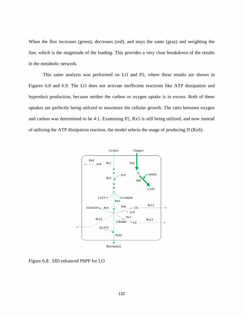
132

When the flux increases (green), decreases (red), and stays the same (gray) and weighting the

line, which is the magnitude of the loading. This provides a very clear breakdown of the results

in the metabolic network.

This same analysis was performed on LO and P2, where these results are shown in

Figures 6.8 and 6.9. The LO does not activate inefficient reactions like ATP dissipation and

byproduct production, because neither the carbon or oxygen uptake is in excess. Both of these

uptakes are perfectly being utilized to maximize the cellular growth. The ratio between oxygen

and carbon was determined to be 4:1. Examining P2, Rx5 is still being utilized, and now instead

of utilizing the ATP dissipation reaction, the model selects the usage of producing D (Rx6).

Figure 6.8: SID enhanced PhPP for LO

133

Figure 6.9: SID enhanced PhPP for P2

Figure 6.10 shows the comparison of P1, LO, and P2 as carbon is varied, and emphasizing the

differences between the phenotypes.

Figure 6.10: Comparison of P1, LO, and P2

C O

134

Figure 6.11: SID enhanced PhPP for P3

Figure 6.11 displays the visualization results for P3, when carbon and oxygen pickup rates were

being varied. Rx5 is turned off, and now the byproduct E is generated by Rx7. The byproduct D

is still being produced and this is negatively correlated with byproduct E, where the direction

depends on whether carbon or oxygen uptake is varied. Table 6.2 shows the shadow prices for P3

and P4. Again, shadow prices that are either zero or positive are easy to interpret, but the others

do not give much information. D and E are zero, meaning that they are expelled from the model

network and NADH is positive, which entails that it is in excess. This explains why Rx5 was

shut off, due to not needing anymore NADH.

Table 6.2: Shadow prices of P3 and P4

Phenotypes A B C D E O2 NADH ATP

P3 -0.05 -0.14 -0.09 0 0 -0.23 0.05 -0.09

P4 0.50 0.50 -1.00 -0.33 0 -0.50 -0.50 0

C O

135

Figure 6.12: SID enhanced PhPP for P4

Figure 6.12 displays the SID enhanced PhPP analysis results for the final phenotype P4.

This phenotype is characterized by carbon being in excess, which is why ATP dissipation

reaction is activated. Also when the carbon uptake rate is increased this causes the biomass

reaction to decrease. The byproduct D is not being produced, but the byproduct E is still in

production. The shadow prices of A and B are positive meaning that they are in excess that is

translated to an excess of carbon. E and ATP are zero, where this is agreement with SID

enhanced PhPP analysis.

In summary, with this simple model network, the newly developed approach of SID

enhanced PhPP analysis supersedes the commonly method of PhPP analysis. Shadow prices

alone cannot extract the fine details of the model network. Although shadow prices can exert

information about whether metabolites are being secreted or if a metabolite is in excess, but it

cannot depict the magnitude of how each reaction is being affected. Overall, SID enhanced PhPP

analysis extracts embedded metabolic information that is known from examining the shadow

prices.

C O

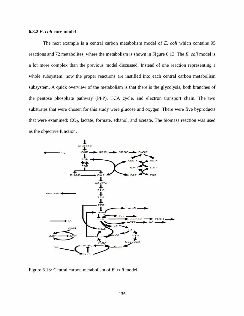
136

6.3.2 E. coli core model

The next example is a central carbon metabolism model of E. coli which contains 95

reactions and 72 metabolites, where the metabolism is shown in Figure 6.13. The E. coli model is

a lot more complex than the previous model discussed. Instead of one reaction representing a

whole subsystem, now the proper reactions are instilled into each central carbon metabolism

subsystem. A quick overview of the metabolism is that there is the glycolysis, both branches of

the pentose phosphate pathway (PPP), TCA cycle, and electron transport chain. The two

substrates that were chosen for this study were glucose and oxygen. There were five byproducts

that were examined: CO2, lactate, formate, ethanol, and acetate. The biomass reaction was used

as the objective function.

Figure 6.13: Central carbon metabolism of E. coli model

137

PhPP analysis was conducted on the E. coli model, where 4 phenotypes were uncovered, P1, P2,

P3, and P4, which is shown in Figure 6.14 (a). When SID enhanced PhPP analysis was carried

out, there was additional phenotypes that was discovered, naming them P3’ and P3”, which is

shown in Figure 6.14 (b). PhPP analysis condenses P3’ and P3’’ into one phenotype (P3), where

the green region in Figure 6.14 emphasizes the differences. The phenotypes P3’ and P3’’ were

detected from the PC scores, which are shown in Figure 6.15.

Figure 6.14: Comparison of phenotypes from PhPP analysis and SID enhanced PhPP analysis.

(a) Phenotypes generated through PhPP analysis and (b) Phenotypes generated through SID

enhanced PhPP analysis.

Figure 6.15 (a) displays the cuts that were made in both the glucose and oxygen uptake direction.

The red arrow represents as glucose uptake is varying, where Figure 6.15 (b) shows the PC score

plot showing the two separate phases, which is due to the break in the linear segment of P3’. The

same is true for the oxygen uptake, which is the blue arrow and Figure 6.15 (c) exhibits the two

different phases. The reason that PhPP analysis was unable to distinguish between P3’ and P3”,

was because the shadow prices are the same in the two phenotypes. It is evident from Figure 6.15

that the PC score is a more reliable measurement to identify the phenotypes.

a b

138

Figure 6.15 SID enhanced PhPP analysis P3’ and P3’’. (a) Cuts in glucose and oxygen direction

in P3’ and P3’’, (b) Disctinction of phenotypes when varying glucose, (c) Disctinction of

phenotypes when varying oxygen.

Figure 6.16 shows the results from SID enhanced PhPP analysis for P3’ and P3’’ when oxygen is

being varied, where the blue dots correspond to reactions that differ in terms of being active or

not active. There are a plethora of differences between the two phenotypes.

Figure 6.16: Comparison of SID enhanced PhPP results of P3’ and P3’’-1. Oxygen uptake is

being varied.

-20 -15 -10 -5 0 5 10 153.5

4

4.5

5

5.5

6

6.5

7

7.5

8

PC Score

Ox

yg

en

Flu

x

P3" P3'

a b c

P3’ P3’’

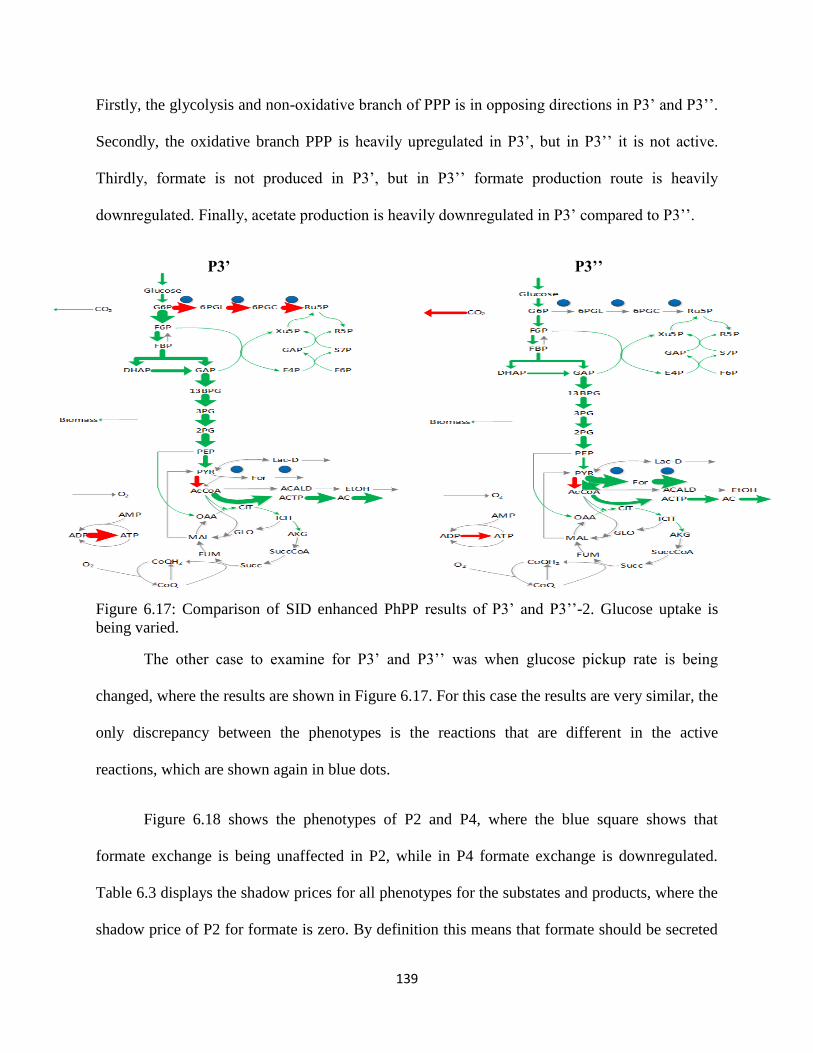
139

Firstly, the glycolysis and non-oxidative branch of PPP is in opposing directions in P3’ and P3’’.

Secondly, the oxidative branch PPP is heavily upregulated in P3’, but in P3’’ it is not active.

Thirdly, formate is not produced in P3’, but in P3’’ formate production route is heavily

downregulated. Finally, acetate production is heavily downregulated in P3’ compared to P3’’.

Figure 6.17: Comparison of SID enhanced PhPP results of P3’ and P3’’-2. Glucose uptake is

being varied.

The other case to examine for P3’ and P3’’ was when glucose pickup rate is being

changed, where the results are shown in Figure 6.17. For this case the results are very similar, the

only discrepancy between the phenotypes is the reactions that are different in the active

reactions, which are shown again in blue dots.

Figure 6.18 shows the phenotypes of P2 and P4, where the blue square shows that

formate exchange is being unaffected in P2, while in P4 formate exchange is downregulated.

Table 6.3 displays the shadow prices for all phenotypes for the substates and products, where the

shadow price of P2 for formate is zero. By definition this means that formate should be secreted

P3’ P3’’

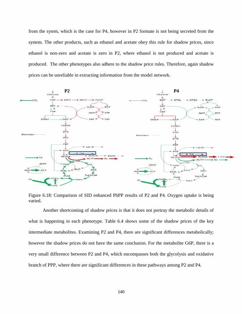
140

from the sytem, which is the case for P4, however in P2 formate is not being secreted from the

system. The other products, such as ethanol and acetate obey this rule for shadow prices, since

ethanol is non-zero and acetate is zero in P2, where ethanol is not produced and acetate is

produced. The other phenotypes also adhere to the shadow price rules. Therefore, again shadow

prices can be unreliable in extracting information from the model network.

Figure 6.18: Comparison of SID enhanced PhPP results of P2 and P4. Oxygen uptake is being

varied.

Another shortcoming of shadow prices is that it does not portray the metabolic details of

what is happening in each phenotype. Table 6.4 shows some of the shadow prices of the key

intermediate metabolites. Examining P2 and P4, there are significant differences metabolically;

however the shadow prices do not have the same conclusion. For the metabolite G6P, there is a

very small difference between P2 and P4, which encompasses both the glycolysis and oxidative

branch of PPP, where there are significant differences in these pathways among P2 and P4.

P2 P4

141

Table 6.3: Shadow prices of the substrates and products for all phenotypes for E. coli.

This is also seen in the E4P, which is a metabolite in the non-oxidative branch of PPP.

Investigating the behavior of the TCA cycle between P2 and P4, we see that the TCA cycle in P2

is fully activated and in P4 it is branched. The metabolite AKG in the TCA cycle shows that the

shadow prices between P2 and P4 are very analogous. Lastly, pyruvate (PYR) has a lot of

interconnections between subsystems, the again the shadow prices of PYR between P2 and P4

are very similar. Looking at the SID enhanced PhPP analysis results there are substantial

differences that are connected to pyruvate. Pyruvate dehydrogenase is the reaction that converts

pyruvate to acetyl-CoA, in P2 this reaction is downregulated, while in P4 this reaction is not

active. Pyruvate is alo involved in for the production of formate, in P4 formate exchange is

downregulated and in P2 formate exchange is non-active.

Table 6.4: Shadow prices of the intermediate metabolites for all phenotypes for E. coli.

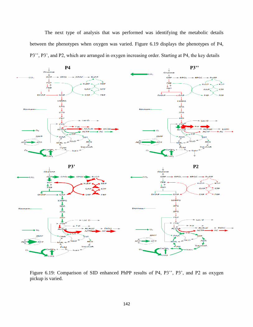
142

The next type of analysis that was performed was identifying the metabolic details

between the phenotypes when oxygen was varied. Figure 6.19 displays the phenotypes of P4,

P3’’, P3’, and P2, which are arranged in oxygen increasing order. Starting at P4, the key details

Figure 6.19: Comparison of SID enhanced PhPP results of P4, P3’’, P3’, and P2 as oxygen

pickup is varied.

P4 P3’’

P3’ P2

143

is that the oxidative branch of PPP is non-active. Glycolysis is downregulated and the non-

oxidative branch of PPP is upregulated. Being a lower oxygen phenotype this caused the TCA

cycle to be branched. There are 4 byproducts being generated: formate, ethanol, and CO2 are

downregulated, while acetate is upregulated. Moving to P3’’, glycolysis, both branches of the

PPP, and the TCA cycle are in the same direction. Ethanol production has now halted, formate is

heavily downregulated, and acetate has switched production direction. Pyruvate dehydrogenase

is now active. In P3’, major changes occur; now the oxidative branch of PPP is activated, which

causes the glycolysis pathway and non-oxidative branch of PPP to be shifted in a different

direction than the previous phenotypes. Formate production has ceased and acetate is now

heavily down regulated. The one similarity between the previous phenotypes is the TCA cycle is

branched. Pyruvate dehydrogenase is now downregulated. Finally in P2, glycolysis and the non-

oxidative branch of PPP is reverted back to the directions of P3’’and P4. The oxidative branch of

PPP is downregulated. The TCA cycle is fully activated denoted that is now in an aerobic phase.

Some similarities between P2 and the previous phenotype of P3’ is that pyruvate dehydrogenase

and acetate production are in the same direction.

6.4 Conclusion

PhPP analysis is a constraint-based tool to characterize different phenotype phases based

on genome-scale models, but its interpretation of different phases based on shadow price is not

straight forward. The SID enhanced PhPP analysis reduces required computation, improves

accuracy, as well as automate the analysis procedure. The key differences between different

phenotype phases can be easily identified through the system identification enhanced approach.

The illustrative example provided a simple model system of how system identification enhanced

PhPP analysis infers the metabolic differences between phases. The E. coli core model was a

144

larger model that shows that only looking at the shadow prices of the metabolites is makes it

very difficult to extract the key metabolic details. The system identification enhanced PhPP

analysis was able to uncover the essential metabolic information for each phase and come up

with correlation between the metabolic pathways.

145

Chapter 7: Conclusion and Outlook

7.1 Conclusion

With the constriction that fossil fuels play on the world wide economy and environment,

alternative fuels are generated to alleviate these growing worries. Renewable energy in the form

of lignocellulosic bioethanol offers a promising substitute, because the feedstock does not

compete with food quantity and there is an abundance supply. However, there are main problem

that needs to be resolved is improving the biological conversion of pentose sugars, most

importantly xylose into bioethanol.

S. stipitis is the most effective strain for native xylose fermentation. Instead of studying

the strain through the commonly used reductionist approach that examines individual elements

one at a time, a system biology approach was taken that investigates the metabolism holistically.

In order to achieve a clear perspective of the relationship between genotypic and phenotypic

behaviors, constraint-based modeling was used to try to dissect this relationship via the

utilization of genome-scale metabolic models. The computational that was employed to the

GSMMs was flux balance analysis.

Once validated, GSMMs provide a platform to effectively interrogate cellular

metabolism, such as characterizing metabolic resource allocation, predicting phenotype,

designing experiments to verify model predictions, as well as designing mutant strains with

desired properties. More importantly, GSMMs allow systematic assessment of how a genetic or

environmental perturbation would affect the organism as a whole.

Validation and evaluation of GSMMs is one of the most challenging tasks in systems

biology, due to the scale and complexity involved in genome-scale metabolisms. The

146

conventional GSMM validation relies on a “point-matching” approach by comparing model

predictions with experimental measurements (usually substrate pickup rates, product secretion

rates and cell growth rate) under different conditions. Due to the scale and complexity involved

in GSMMs, combinations of multiple errors in a model could produce good agreement between

predicted and measured fluxes over different points. In addition, it is very difficult to pinpoint the

potential root cause (e.g., specific reactions) if erroneous model predictions occur, and model

refinement requires significant effort from the modeler to manually examine hundreds or

thousands of reactions

A novel system identification based (SID-based) framework was developed in order to

enable a knowledge-matching approach for GSMM validation. In essence, a high-quality

GSMMs is a comprehensive and well-annotated knowledge base of the strain’s cellular

metabolism. In the SID-based framework, the knowledge embedded in a GSMM is extracted

through designed in silico experiments, and model validation is done by matching the extracted

knowledge with the existing knowledge. We have applied the SID-based framework to conduct a

comprehensive evaluation of the two published models, iSS884 and iBB814, and concluded that

although both models contain multiple errors, biological knowledge captured by iBB814 agree

better with existing knowledge on S. stiptis.

Regarding GSMM refinement, one major challenge is how to identify what reactions in

the model should be modified, what reactions should be added to the model and what reactions

should be deleted from the model, in order to obtain desired model behavior. Because the

interconnectivity in the metabolic networks, many times seemingly unrelated reactions located

far away from the “problematic” reactions, i.e., reactions that are not carried out in the way as

expected, play a key role in changing model behavior. As a result, most of the time GSMM

147

refinement is through trial-and-error, and relies heavily on the modeler’s knowledge and

capability to sort out clues from various simulation results; and model refine is usually labor

intensive and time consuming. In this work, we extend the SID-based framework to guide model

refinement, and report an improved GSMM on S. stipitis, iAD828. The improved model predicts

the production of an important byproduct, xylitol, under oxygen-limited conditions, which agrees

with experimental observations. Note that both iSS884 and iBB814 fails in predicting xylitol

production under such conditions. In addition, the analysis performed using the SID-based

framework confirms that iAD828 offer better agreement with existing knowledge on S. stipitis

than iSS884 and iBB814.

Due to the metabolic advancements of iAD828, cofactor engineering strategies was

applied in order to force carbon flux toward ethanol overproduction. The cofactor preference of

xylose reductase was varied and an optimal phenotype was determined. Analysis from this

guided metabolic engineering in silico strategies, which resulted in elevated production of

ethanol.

The SID framework was not only used for validation and refinement of GSMMs, but was

used to enhance phenotype phase plane analysis. SID enhanced PhPP analysis was a

methodology that was developed and applied to an illustrated example and E. coli core model in

order to show the power of uncovering the metabolic information that the traditional PhPP

analysis fails to do. The traditional PhPP analysis used shadow prices to determine the different

phenotypes, which showed to be problematic for the E. coli core model. SID enhanced PhPP

analysis was able to detect a “missing” phenotype that PhPP analysis failed to uncover. Also as

the size of the metabolic model increases, the shadow price from PhPP analysis now provided

148

miniscule meaning. Error was shown in the shadow price of the formate exchange flux. SID

enhanced PhPP analysis provides a powerful tool for understanding metabolic phenotypes.

7.2 Outlook

Even though advancements were made to iAD828, there are still limitations that hinder

the performance:

Acetic Acid production: Wet lab experiments show that acetic acid was produced

simultaneously with xylitol under oxygen-limited condition. There is a redox balance issue here,

but in order for this to happen there might need to be regulation schemes implemented.

Robustness: iAD828 did add improvement, but there were additional phenotypes added under

both oxygen-limited and aerobic condition. The number of phenotypes on both sides of the

spectrum for oxygen needs to be cut back.

Biomass/Objective function: The biomass formation equation from iBB814 was used as the

objective function. Additionally experiments could be done to make the biomass formation

equation more accurate. iSS884 showed a lot of fatty acids that were absent from iBB814

biomass equation. Also does the biomass formation equation change with oxygen level.

Metabolic engineering for ethanol overproduction is performed under oxygen-limited condition,

collect data under this condition for biomass for be very helpful. Another part of this is to try

different objective functions, such as the redox power, but also combine objective functions

together.

Metabolic engineering: There are numerous of tools that have developed for overproduction of

a desired metabolite. Use these to develop metabolic engineering strategies, these could allow

biologist with ways to increase xylose fermentation.

149

Anaerobic growth: S. stipitis fails to grow under anaerobic conditions, thus it would be very

advantageous to discover the reason(s) for this.

Dynamic modeling: The modeling used here employs the steady state assumption, using kinetic

modeling or optimal control approaches would be very beneficial to model dynamic processes

such as batch and fed batch, which is the majority of the operations scheme in industry.

150

Bibliography

Global Status Report - REN21. (2014). Retrieved October 19, 2015.

IEA. World energy outlook world energy outlook. Paris: International Energy Agency; 2007.

Iowa State Univeristy. Thrust 2: Microbial Metabolic Engineering. (2008). Retrieved October 1, 2015:

http://www.cbirc.iastate.edu/research/thrust2/

Aderem, A. (2005). Systems biology: its practice and challenges. Cell, 121(4), 511-513

Agbogbo, F. K., & Coward-Kelly, G. (2008). Cellulosic ethanol production using the naturally

occurring xylose-fermenting yeast, Pichia stipitis. Biotechnology letters, 30(9), 1515-1524.

Anesiadis, N., Cluett, W. R., & Mahadevan, R. (2008). Dynamic metabolic engineering for

increasing bioprocess productivity. Metabolic engineering, 10(5), 255-266.

Antoniewicz, M. R. (2013). Dynamic metabolic flux analysis—tools for probing transient states

of metabolic networks. Current opinion in biotechnology, 24(6), 973-978.

Balagurunathan, B., Jonnalagadda, S., Tan, L., & Srinivasan, R. (2012). Reconstruction and

analysis of a genome-scale metabolic model for Scheffersomyces stipitis. Microb Cell Fact,

11(1), 27.

Balan, V. (2014). Current Challenges in Commercially Producing Biofuels from Lignocellulosic

Biomass. ISRN Biotechnology, 1-31.

Balat, M., & Balat, H. (2009). Recent trends in global production and utilization of bio-ethanol

fuel. Applied Energy, 2273-2282.

Balkema, A., & Pols, A. (2015). Biofuels: Sustainable Innovation or Gold Rush? Identifying

Responsibilities for Biofuel Innovations. Responsible Innovation 2, 283-303.

Barabasi, A. L., & Oltvai, Z. N. (2004). Network biology: understanding the cell's functional

organization. Nature reviews genetics, 5(2), 101-113.

Becker, S. A., Feist, A. M., Mo, M. L., Hannum, G., Palsson, B. Ø., & Herrgard, M. J. (2007).

Quantitative prediction of cellular metabolism with constraint-based models: the COBRA

Toolbox. Nature protocols, 2(3), 727-738.

Bell, S. L., & Palsson, B. Ø. (2005). Phenotype phase plane analysis using interior point

methods. Computers & chemical engineering, 29(3), 481-486.

Berezina, O. V., Zakharova, N. V., Brandt, A., Yarotsky, S. V., Schwarz, W. H., & Zverlov, V.

(2010). Reconstructing the clostridial n-butanol metabolic pathway in Lactobacillus brevis.

Applied microbiology and biotechnology, 87(2), 635-646.

151

Berg C, World bioethanol production, the distillery and bioethanol network. Available from:

http://www.distill.com/worldethanolproduction.htm; 2001.

Bjerre, A., Olesen, A., Fernqvist, T., Plöger, A., & Schmidt, A. (1996). Pretreatment of wheat

straw using combined wet oxidation and alkaline hydrolysis resulting in convertible

cellulose and hemicellulose. Biotechnol. Bioeng. Biotechnology and Bioengineering, 568-

577.

Bordbar, A., Monk, J. M., King, Z. A., & Palsson, B. O. (2014). Constraint-based models predict

metabolic and associated cellular functions. Nature Reviews Genetics, 15(2), 107-120.

Bruinenberg, P. M., de Bot, P. H., van Dijken, J. P., & Scheffers, W. A. (1984). NADH-linked

aldose reductase: the key to anaerobic alcoholic fermentation of xylose by yeasts. Applied

microbiology and biotechnology, 19(4), 256-260.

Borden, J. R., Jones, S. W., Indurthi, D., Chen, Y., & Papoutsakis, E. T. (2010). A genomic-

library based discovery of a novel, possibly synthetic, acid-tolerance mechanism in

Clostridium acetobutylicum involving non-coding RNAs and ribosomal RNA processing.

Metabolic engineering, 12(3), 268-281.

Bro, C., Regenberg, B., Förster, J., & Nielsen, J. (2006). In silico aided metabolic engineering of

Saccharomyces cerevisiae for improved bioethanol production. Metabolic engineering, 8(2),

102-111.

Bruinenberg, P. M., Van Dijken, J. P., & Scheffers, W. A. (1983). An enzymic analysis of

NADPH production and consumption in Candida utilis. Journal of General Microbiology,

129(4), 965-971.

Burgard, A. P., Pharkya, P., & Maranas, C. D. (2003). Optknock: a bilevel programming

framework for identifying gene knockout strategies for microbial strain optimization.

Biotechnology and bioengineering, 84(6), 647-657.

Caspeta, L., Shoaie, S., Agren, R., Nookaew, I., & Nielsen, J. (2012). Genome-scale metabolic

reconstructions of Pichia stipitis and Pichia pastoris and in silico evaluation of their

potentials. BMC systems biology, 6(1), 24.

Cherubini, F. (2010). The biorefinery concept: Using biomass instead of oil for producing energy

and chemicals. Energy Conversion and Management, 51(7), 1412–1421.

Cho, J. Y., & Jeffries, T. W. (1998). Pichia stipitis genes for alcohol dehydrogenase with

fermentative and respiratory functions. Applied and environmental microbiology, 64(4),

1350-1358.

152

Cho, J. Y., & Jeffries, T. W. (1999). Transcriptional control of ADH genes in the xylose-

fermenting yeast Pichia stipitis. Applied and environmental microbiology, 65(6), 2363-2368.

Collins K (2007). The new world of biofuels: implications for agriculture and energy. Energy

Information Administration (United States Department of Energy) Energy Outlook,

Modeling, and Data Conference. 28 March.

Covert, M. W., Schilling, C. H., Famili, I., Edwards, J. S., Goryanin, I. I., Selkov, E., & Palsson,

B. O. (2001). Metabolic modeling of microbial strains in silico. Trends in biochemical

sciences, 26(3), 179-186.

Cvijovic, M., Olivares-Hernández, R., Agren, R., Dahr, N., Vongsangnak, W., Nookaew, I., &

Nielsen, J. (2010). BioMet Toolbox: genome-wide analysis of metabolism. Nucleic acids

research, 38(suppl 2), W144-W149

Dahn, K. M., Davis, B. P., Pittman, P. E., Kenealy, W. R., & Jeffries, T. W. (1996, January).

Increased xylose reductase activity in the xylose-fermenting yeast Pichia stipitis by

overexpression of XYL1. In Seventeenth Symposium on Biotechnology for Fuels and

Chemicals (pp. 267-276). Humana Press.

Damiani, A. L., He, Q. P., Jeffries, T. W., & Wang, J. (2015). Comprehensive evaluation of two

genome‐scale metabolic network models for Scheffersomyces stipitis. Biotechnology and

bioengineering, 112(6), 1250-1262.

Daran-Lapujade, P., Rossell, S., van Gulik, W. M., Luttik, M. A., de Groot, M. J., Slijper, M., &

Bakker, B. M. (2007). The fluxes through glycolytic enzymes in Saccharomyces cerevisiae

are predominantly regulated at posttranscriptional levels. Proceedings of the National

Academy of Sciences, 104(40), 15753-15758.

De Deken, R. H. (1966). The Crabtree effect and its relation to the petite mutation. Journal of

general microbiology, 44(2), 157-165

Du Preez, J. C., Van Driessel, B., & Prior, B. A. (1989). Effect of aerobiosis on fermentation and

key enzyme levels during growth of Pichia stipitis, Candida shehatae and Candida tenuis on

D-xylose. Archives of microbiology, 152(2), 143-147.

Du Preez, J. C., Van Driessel, B., & Prior, B. A. (1989). Ethanol tolerance of Pichia stipitis and

Candida shehatae strains in fed-batch cultures at controlled low dissolved oxygen levels.

Applied microbiology and biotechnology, 30(1), 53-58.

Duarte, N. C., Palsson, B. Ø., & Fu, P. (2004). Integrated analysis of metabolic phenotypes in

Saccharomyces cerevisiae. BMC genomics, 5(1), 63.

Edwards, J. S., & Palsson, B. O. (2000). Robustness analysis of the escherichiacoli metabolic

network. Biotechnology Progress, 16(6), 927-939.

153

Edwards, J. S., Ibarra, R. U., & Palsson, B. O. (2001). In silico predictions of Escherichia coli

metabolic capabilities are consistent with experimental data. Nature biotechnology, 19(2),

125-130.

Edwards, J. S., Covert, M., & Palsson, B. (2002a). Metabolic modelling of microbes: the flux‐

balance approach. Environmental microbiology, 4(3), 133-140.

Edwards, J. S., Ramakrishna, R., & Palsson, B. O. (2002b). Characterizing the metabolic

phenotype: a phenotype phase plane analysis. Biotechnology and bioengineering, 77(1), 27-

36.

Eisentraut, A. (2010). Sustainable Production of Second-Generation Biofuels. IEA Energy

Papers.

Eliasson, A., Christensson, C., Wahlbom, C. F., & Hahn-Hägerdal, B. (2000). Anaerobic xylose

fermentation by recombinant Saccharomyces cerevisiae carrying XYL1, XYL2, andXKS1

in mineral medium chemostat cultures. Applied and Environmental Microbiology, 66(8),

3381-3386

Evans, M. (1997). The economic impact of the demand for ethanol. Lombard, Ill.: Midwestern

Governors' Conference.

Famili, I., Mahadevan, R., & Palsson, B. O. (2005). k-Cone analysis: determining all candidate

values for kinetic parameters on a network scale. Biophysical journal, 88(3), 1616-1625

Feist, A. M., Herrgård, M. J., Thiele, I., Reed, J. L., & Palsson, B. Ø. (2009). Reconstruction of

biochemical networks in microorganisms. Nature Reviews Microbiology, 7(2), 129-143.

Feist, A. M., & Palsson, B. O. (2010). The biomass objective function. Current opinion in

microbiology, 13(3), 344-349.

Fell, D. A., & Small, J. R. (1986). Fat synthesis in adipose tissue. An examination of

stoichiometric constraints. Biochem. J, 238, 781-786.

Galitski, T. (2012, March 15). Reductionism Gives Way to Systems Biology | GEN Magazine

Articles | GEN. Retrieved September 29, 2015.

Gallagher, R., Appenzeller, T., & Normile, D. (1999). Beyond reductionism. Science, 284(5411),

79.

Gianchandani, E. P., Chavali, A. K., & Papin, J. A. (2010). The application of flux balance

analysis in systems biology. Wiley Interdisciplinary Reviews: Systems Biology and

Medicine, 2(3), 372-382.

154

Gírio, F., Fonseca, C., Carvalheiro, F., Duarte, L., Marques, S., & Bogel-Łukasik, R. (2010).

Hemicelluloses for fuel ethanol: A review. Bioresource Technology, 4775-4800.

Grootjen, D. R. J., Van der Lans, R. G. J. M., & Luyben, K. C. A. (1990). Effects of the aeration

rate on the fermentation of glucose and xylose by Pichia stipitis CBS 5773. Enzyme and

microbial technology, 12(1), 20-23.

Grootjen, D. R. J., van Der Lans, R. G. J. M., & Luyben, K. C. A. (1991). Conversion of

glucose/xylose mixtures by Pichia stipitis under oxygen-limited conditions. Enzyme and

microbial technology, 13(8), 648-654.

Gstaiger, M., & Aebersold, R. (2009). Applying mass spectrometry-based proteomics to

genetics, genomics and network biology. Nature Reviews Genetics, 10(9), 617-627

Gudmundsson, S., & Thiele, I. (2010). Computationally efficient flux variability analysis. BMC

bioinformatics, 11(1), 489.

Gupta, A., & Verma, J. P. (2015). Sustainable bio-ethanol production from agro-residues: A

review. Renewable and Sustainable Energy Reviews, 41, 550–567.

Ideker, T., Galitski, T., & Hood, L. (2001). A new approach to decoding life: systems biology.

Annual review of genomics and human genetics, 2(1), 343-372.

Hahn-Hägerdal, B., & Pamment, N. (2004). Special session A microbial pentose metabolism.

Applied biochemistry and biotechnology, 116(1), 1207-1209.

Hahn-Hägerdal, B., Karhumaa, K., Fonseca, C., Spencer-Martins, I., & Gorwa-Grauslund, M. F.

(2007). Towards industrial pentose-fermenting yeast strains. Applied microbiology and

biotechnology, 74(5), 937-953.

Hakeem, K. (2014). Biomass and bioenergy: Applications.

Hanly, T. J., & Henson, M. A. (2011). Dynamic flux balance modeling of microbial co‐cultures

for efficient batch fermentation of glucose and xylose mixtures. Biotechnology and

bioengineering, 108(2), 376-385.

Harhangi, H. R., Akhmanova, A. S., Emmens, R., van der Drift, C., de Laat, W. T., van Dijken,

J. P., & den Camp, H. J. O. (2003). Xylose metabolism in the anaerobic fungus Piromyces

sp. strain E2 follows the bacterial pathway. Archives of Microbiology, 180(2), 134-141.

Hearst, M. A., Dumais, S. T., Osman, E., Platt, J., & Scholkopf, B. (1998). Support vector

machines. Intelligent Systems and their Applications, IEEE, 13(4), 18-28.

Henry, C. S., DeJongh, M., Best, A. A., Frybarger, P. M., Linsay, B., & Stevens, R. L. (2010).

High-throughput generation, optimization and analysis of genome-scale metabolic models.

Nature biotechnology, 28(9), 977-982.

155

Heux, S., Cachon, R., & Dequin, S. (2006). Cofactor engineering in Saccharomyces cerevisiae:

expression of a H 2 O-forming NADH oxidase and impact on redox metabolism. Metabolic

engineering, 8(4), 303-314.

Hjersted, J. L., & Henson, M. A. (2009). Steady-state and dynamic flux balance analysis of

ethanol production by Saccharomyces cerevisiae. IET systems biology, 3(3), 167-179.

Hou, J., Lages, N. F., Oldiges, M., & Vemuri, G. N. (2009). Metabolic impact of redox cofactor

perturbations in Saccharomyces cerevisiae. Metabolic engineering, 11(4), 253-261.

Hufbauer, G., & Charnovitz, S. (2009). Global warming and the world trading system (pp. 6-8).

Washington, D.C.: Peterson Institute for International Economics.

Jamshidi, N., & Palsson, B. Ø. (2008). Formulating genome‐scale kinetic models in the post‐genome era. Molecular systems biology, 4(1), 171.

Jeffries, T. W., & Shi, N. Q. (1999). Genetic engineering for improved xylose fermentation by

yeasts. In Recent progress in bioconversion of lignocellulosics (pp. 117-161). Springer

Berlin Heidelberg.

Jeffries, T. W. (2006). Engineering yeasts for xylose metabolism. Current opinion in

biotechnology, 17(3), 320-326.

Jeffries, T. W., Grigoriev, I. V., Grimwood, J., Laplaza, J. M., Aerts, A., Salamov, A., &

Richardson, P. M. (2007). Genome sequence of the lignocellulose-bioconverting and

xylose-fermenting yeast Pichia stipitis. Nature biotechnology, 25(3), 319-326.

Jeffries, T. W., & Van Vleet, J. R. H. (2009). Pichia stipitis genomics, transcriptomics, and gene

clusters. FEMS yeast research, 9(6), 793-807.

Jeppsson, M., Johansson, B., Hahn-Hägerdal, B., & Gorwa-Grauslund, M. F. (2002). Reduced

oxidative pentose phosphate pathway flux in recombinant xylose-utilizing Saccharomyces

cerevisiae strains improves the ethanol yield from xylose. Applied and environmental

microbiology, 68(4), 1604-1609.

Joachimsthal, E., & Rogers, P. (2000). Characterization of a High-Productivity Recombinant

Strain of Zymomonas mobilis for Ethanol Production from Glucose/Xylose Mixtures.

Twenty-First Symposium on Biotechnology for Fuels and Chemicals, 343-356.

Johansson, B., & Hahn‐Hägerdal, B. (2002). The non‐oxidative pentose phosphate pathway

controls the fermentation rate of xylulose but not of xylose in Saccharomyces cerevisiae

TMB3001. FEMS yeast research, 2(3), 277-282

Joseph‐Horne, T., & Hollomon, D. W. (2000). Functional diversity within the mitochondrial

electron transport chain of plant pathogenic fungi. Pest Management Science, 56(1), 24-30.

156

Kanehisa, M., & Goto, S. (2000). KEGG: kyoto encyclopedia of genes and genomes. Nucleic

acids research, 28(1), 27-30.

Karhumaa, K., Hahn‐Hägerdal, B., & Gorwa‐Grauslund, M. F. (2005). Investigation of limiting

metabolic steps in the utilization of xylose by recombinant Saccharomyces cerevisiae using

metabolic engineering. Yeast, 22(5), 359-368

Karhumaa, K., Sanchez, R. G., Hahn-Hägerdal, B., & Gorwa-Grauslund, M. F. (2007).

Comparison of the xylose reductase-xylitol dehydrogenase and the xylose isomerase

pathways for xylose fermentation by recombinant Saccharomyces cerevisiae. Microbial

Cell Factories, 6(1), 5.

Karp, P. D., Riley, M., Paley, S. M., & Pellegrini-Toole, A. (2002). The metacyc database.

Nucleic acids research, 30(1), 59-61.

Karr, J. R., Sanghvi, J. C., Macklin, D. N., Gutschow, M. V., Jacobs, J. M., Bolival, B., &

Covert, M. W. (2012). A whole-cell computational model predicts phenotype from

genotype. Cell, 150(2), 389-401.

Katahira, S., Ito, M., Takema, H., Fujita, Y., Tanino, T., Tanaka, T., ... & Kondo, A. (2008).

Improvement of ethanol productivity during xylose and glucose co-fermentation by xylose-

assimilating S. cerevisiae via expression of glucose transporter Sut1. Enzyme and Microbial

Technology, 43(2), 115-119.

Kauffman, K. J., Prakash, P., & Edwards, J. S. (2003). Advances in flux balance analysis.

Current opinion in biotechnology, 14(5), 491-496.

Kim, Y., Ingram, L., & Shanmugam, K. (2007). Construction of an Escherichia coli K-12 Mutant

for Homoethanologenic Fermentation of Glucose or Xylose without Foreign Genes.

APPLIED AND ENVIRONMENTAL MICROBIOLOGY, 1766-1771.

Kim, T. Y., Sohn, S. B., Kim, Y. B., Kim, W. J., & Lee, S. Y. (2012). Recent advances in

reconstruction and applications of genome-scale metabolic models. Current opinion in

biotechnology, 23(4), 617-623.

Kim, M. H. (2015). New Experimental and Modeling Approaches to Study the Dynamics of

Xylose Fermenta-tion with Scheffersomyces stipitis (Doctoral dissertation, Auburn

University).

King, Z. A., Lloyd, C. J., Feist, A. M., & Palsson, B. O. (2015). Next-generation genome-scale

models for metabolic engineering. Current opinion in biotechnology, 35, 23-29.

Kitano, H. (2002). Systems Biology: A Brief Overview. Science, 1662-1664.

157

Klamt, S., & Stelling, J. (2003). Two approaches for metabolic pathway analysis?. Trends in

biotechnology, 21(2), 64-69.

Klapa, M. I., & Stephanopoulos, G. (2000). Metabolic flux analysis. In Bioreaction Engineering

(pp. 106-124). Springer Berlin Heidelberg.

Klinner, U., Fluthgraf, S., Freese, S., & Passoth, V. (2005). Aerobic induction of respiro-

fermentative growth by decreasing oxygen tensions in the respiratory yeast Pichia stipitis.

Applied microbiology and biotechnology, 67(2), 247-253.

Kompala, D. S., Ramkrishna, D., & Tsao, G. T. (1984). Cybernetic modeling of microbial

growth on multiple substrates. Biotechnology and bioengineering, 26(11), 1272-1281.

Knorr, A. L., Jain, R., & Srivastava, R. (2007). Bayesian-based selection of metabolic objective

functions. Bioinformatics, 23(3), 351-357.

Kötter, P., & Ciriacy, M. (1993). Xylose fermentation by Saccharomyces cerevisiae. Applied

microbiology and biotechnology, 38(6), 776-783.

Kreutz, C., & Timmer, J. (2009). Systems biology: experimental design. FEBS journal, 276(4),

923-942.

Krömer, J., Quek, L. E., & Nielsen, L. (2009). 13C-Fluxomics: a tool for measuring metabolic

phenotypes. Aust Biochem, 40(3), 17-20.

Krömer, J. O., Nielsen, L. K., & Blank, L. M. (Eds.). (2014). Metabolic Flux Analysis: Methods

and Protocols. Humana Press.

Kuyper, M., Hartog, M. M., Toirkens, M. J., Almering, M. J., Winkler, A. A., Dijken, J. P., &

Pronk, J. T. (2005). Metabolic engineering of a xylose‐isomerase‐expressing

Saccharomyces cerevisiae strain for rapid anaerobic xylose fermentation. FEMS yeast

research, 5(4‐5), 399-409.

Llaneras, F., & Picó, J. (2010). Which metabolic pathways generate and characterize the flux

space? A comparison among elementary modes, extreme pathways and minimal generators.

BioMed Research International, 2010.

Lee, J. M., Gianchandani, E. P., & Papin, J. A. (2006). Flux balance analysis in the era of

metabolomics. Briefings in bioinformatics, 7(2), 140-150.

Lee, K. Y., Park, J. M., Kim, T. Y., Yun, H., & Lee, S. Y. (2010). The genome-scale metabolic

network analysis of Zymomonas mobilis ZM4 explains physiological features and suggests

ethanol and succinic acid production strategies. Microbial cell factories, 9(1), 94.

158

Lee, J. Y., Yang, K. S., Jang, S. A., Sung, B. H., & Kim, S. C. (2011). Engineering butanol‐tolerance in escherichia coli with artificial transcription factor libraries. Biotechnology and

bioengineering, 108(4), 742-749.

Lewis, N. E., Nagarajan, H., & Palsson, B. O. (2012). Constraining the metabolic genotype–

phenotype relationship using a phylogeny of in silico methods. Nature Reviews

Microbiology, 10(4), 291-305.

Li, P. Y. (2012). In silico metabolic network reconstruction of Scheffersomyces stipitis (Doctoral

dissertation)

Liang, M., Damiani, A., He, Q. P., & Wang, J. (2013). Elucidating xylose metabolism of

Scheffersomyces stipitis for lignocellulosic ethanol production. ACS Sustainable Chemistry

& Engineering, 2(1), 38-48.

Licht, F.O., (2006). World Ethanol Market: The Outlook to 2015, Tunbridge Wells, Agra Europe

Special Report, UK.

Licht, F. O. (2013). Renewable fuels association. Ethanol industry outlook 2008–2013 reports.

Liu, L., Agren, R., Bordel, S., & Nielsen, J. (2010). Use of genome-scale metabolic models for

understanding microbial physiology. FEBS letters, 584(12), 2556-2564.

Liu, T., Zou, W., Liu, L., & Chen, J. (2012). A constraint-based model of Scheffersomyces

stipitis for improved ethanol production. Biotechnol Biofuels, 5(1), 72.

Lütke-Eversloh, T., & Bahl, H. (2011). Metabolic engineering of Clostridium acetobutylicum:

recent advances to improve butanol production. Current opinion in biotechnology, 22(5),

634-647.

Mahadevan, R., & Schilling, C. H. (2003). The effects of alternate optimal solutions in

constraint-based genome-scale metabolic models. Metabolic engineering, 5(4), 264-276.

Mahadevan, R., & Henson, M. A. (2007). Genome-scale analysis of Saccharomyces cerevisiae

metabolism and ethanol production in fed-batch culture. Biotechnology and bioengineering,

97(5), 1190-1204

Mansfield, Betty Kay et al. (2006). Breaking the Biological barriers to Cellulosic Ethanol: A

Joint Research Agenda. Tech. rep. Germantown, MD, USA: US DOE

Margeot, A., Hahn-Hagerdal, B., Edlund, M., Slade, R., & Monot, F. (2009). New improvements

for lignocellulosic ethanol. Current opinion in biotechnology, 20(3), 372-380.

Marioni, J. C., Mason, C. E., Mane, S. M., Stephens, M., & Gilad, Y. (2008). RNA-seq: an

assessment of technical reproducibility and comparison with gene expression arrays.

Genome research, 18(9), 1509-1517.

159

Marris, E. (2006). Sugar cane and ethanol: Drink the best and drive the rest. Nature

News@nature, 670-672.

Martı́n, C., Galbe, M., Wahlbom, C. F., Hahn-Hägerdal, B., & Jönsson, L. J. (2002). Ethanol

production from enzymatic hydrolysates of sugarcane bagasse using recombinant xylose-

utilising Saccharomyces cerevisiae. Enzyme and Microbial Technology, 31(3), 274-282.

Matsushika, A., Watanabe, S., Kodaki, T., Makino, K., Inoue, H., Murakami, K., & Sawayama,

S. (2008). Expression of protein engineered NADP+-dependent xylitol dehydrogenase

increases ethanol production from xylose in recombinant Saccharomyces cerevisiae.

Applied microbiology and biotechnology, 81(2), 243-255.

Matsushika, A., Inoue, H., Kodaki, T., & Sawayama, S. (2009a). Ethanol production from xylose

in engineered Saccharomyces cerevisiae strains: current state and perspectives. Applied

Microbiology and Biotechnology, 84(1), 37-53.

Matsushika, A., Inoue, H., Murakami, K., Takimura, O., & Sawayama, S. (2009b). Bioethanol

production performance of five recombinant strains of laboratory and industrial xylose-

fermenting Saccharomyces cerevisiae. Bioresource Technology, 100(8), 2392-2398.

Mavrovouniotis, M., & Stephanopoulos, G. (1992). Synthesis of biochemical production routes.

Computers & chemical engineering, 16(6), 605-619.

Mckendry, P. (2002). Energy production from biomass (part 2): Conversion technologies.

Bioresource Technology, 47-54.

Mockler, T. C., & Ecker, J. R. (2005). Applications of DNA tiling arrays for whole-genome

analysis. Genomics, 85(1), 1-15.

Montagud, A., Navarro, E., de Córdoba, P. F., Urchueguía, J. F., & Patil, K. R. (2010).

Reconstruction and analysis of genome-scale metabolic model of a photosynthetic

bacterium. BMC systems biology, 4(1), 156.

Mousdale, D. (2008). Biofuels: Biotechnology, chemistry, and sustainable development. Boca

Raton: CRC Press.

Naik, S., Goud, V., Rout, P., & Dalai, A. (2009). Production of first and second generation

biofuels: A comprehensive review. Renewable and Sustainable Energy Reviews, 578-597.

Nemutlu, E., Zhang, S., Juranic, N. O., Terzic, A., Macura, S., & Dzeja, P. (2012). 18 O-assisted

dynamic metabolomics for individualized diagnostics and treatment of human diseases.

Croatian medical journal, 53(6), 529-534.

Oberhardt, M. A., Palsson, B. Ø., & Papin, J. A. (2009). Applications of genome‐scale metabolic

reconstructions. Molecular systems biology, 5(1), 320

160

Ohgren, K., Bura, R., Saddler, J., & Zacchi, G. (2007). Effect of hemicellulose and lignin

removal on enzymatic hydrolysis of steam pretreated corn stover. Bioresource Technology,

2503-2510.

Orth, J. D., Thiele, I., & Palsson, B. Ø. (2010a). What is flux balance analysis?. Nature

biotechnology, 28(3), 245-248.

Orth J.D., Fleming, R., & Palsson, B. Ø. (2010b) Reconstruction and Use of Microbial

Metabolic Networks: the Core Escherichia coli Metabolic Model as an Educational Guide

by Orth, Fleming, and Palsson

Orth, J. D., Conrad, T. M., Na, J., Lerman, J. A., Nam, H., Feist, A. M., & Palsson, B. Ø. (2011).

A comprehensive genome‐scale reconstruction of Escherichia coli metabolism—2011.

Molecular systems biology, 7(1), 535.

Österlund, T., Nookaew, I., & Nielsen, J. (2012). Fifteen years of large scale metabolic modeling

of yeast: developments and impacts. Biotechnology advances, 30(5), 979-988.

Paley, S. M., Latendresse, M., & Karp, P. D. (2012). Regulatory network operations in the

pathway tools software. BMC bioinformatics, 13(1), 243

Palsson, B. (2000). The challenges of in silico biology. Nature biotechnology, 18(11), 1147-

1150.

Passoth, V., Zimmermann, M., & Klinner, U. (1996, January). Peculiarities of the regulation of

fermentation and respiration in the Crabtree-negative, xylose-fermenting yeast Pichia

stipitis. In Seventeenth Symposium on Biotechnology for Fuels and Chemicals (pp. 201-

212). Humana Press.

Patil, K. R., Rocha, I., Förster, J., & Nielsen, J. (2005). Evolutionary programming as a platform

for in silico metabolic engineering. BMC bioinformatics, 6(1), 308.

Patiño, C. E. H., Jaime-Muñoz, G., & Resendis-Antonio, O. (2012). Systems biology of cancer:

moving toward the integrative study of the metabolic alterations in cancer cells. Frontiers in

physiology, 3.

Pharkya, P., Burgard, A. P., & Maranas, C. D. (2004). OptStrain: a computational framework for

redesign of microbial production systems. Genome research, 14(11), 2367-2376.

Pramanik, J., & Keasling, J. D. (1997). Stoichiometric model of Escherichia coli metabolism:

incorporation of growth-rate dependent biomass composition and mechanistic energy

requirements. Biotechnology and bioengineering, 56(4), 398-421.

Price, N. D., Reed, J. L., & Palsson, B. Ø. (2004). Genome-scale models of microbial cells:

evaluating the consequences of constraints. Nature Reviews Microbiology, 2(11), 886-897.

161

Ramakrishna, R., Edwards, J. S., McCulloch, A., & Palsson, B. O. (2001). Flux-balance analysis

of mitochondrial energy metabolism: consequences of systemic stoichiometric constraints.

American Journal of Physiology-Regulatory, Integrative and Comparative Physiology,

280(3), R695-R704.

Raman, K., & Chandra, N. (2009). Flux balance analysis of biological systems: applications and

challenges. Briefings in bioinformatics, 10(4), 435-449.

Ranganathan, S., Suthers, P. F., & Maranas, C. D. (2010). OptForce: an optimization procedure

for identifying all genetic manipulations leading to targeted overproductions. PLoS Comput

Biol, 6(4), e1000744.

Reed, J. L. (2012). Shrinking the metabolic solution space using experimental datasets. PLoS

Comput Biol, 8(8), e1002662.

Rizzi, M., Baltes, M., Theobald, U., & Reuss, M. (1997). In vivo analysis of metabolic dynamics

in Saccharomyces cerevisiae: II. mathematical model. Biotechnology and bioengineering,

55(4), 592-608

Roca, C., Nielsen, J., & Olsson, L. (2003). Metabolic engineering of ammonium assimilation in

xylose-fermenting Saccharomyces cerevisiae improves ethanol production. Applied and

environmental microbiology, 69(8), 4732-4736.

Rocha, I., Maia, P., Rocha, M., & Ferreira, E. C. (2008). OptGene: a framework for in silico

metabolic engineering.

Sabido, E., Selevsek, N., & Aebersold, R. (2012). Mass spectrometry-based proteomics for

systems biology. Current opinion in biotechnology, 23(4), 591-597.

Sanford, K., Soucaille, P., Whited, G., & Chotani, G. (2002). Genomics to fluxomics and

physiomics—pathway engineering. Current opinion in microbiology, 5(3), 318-322.

Sauer, U. (2006). Metabolic networks in motion: 13C‐based flux analysis. Molecular systems

biology, 2(1), 62.

Sauer, U., Heinemann, M., & Zamboni, N. (2007). Getting closer to the whole picture.

Science(Washington), 316(5824), 550-551.

Savinell, J. M., & Palsson, B. O. (1992). Network analysis of intermediary metabolism using

linear optimization. I. Development of mathematical formalism. Journal of theoretical

biology, 154(4), 421-454.

Scalbert, A., Brennan, L., Fiehn, O., Hankemeier, T., Kristal, B. S., van Ommen, B., ... &

Wopereis, S. (2009). Mass-spectrometry-based metabolomics: limitations and

recommendations for future progress with particular focus on nutrition research.

Metabolomics, 5(4), 435-458.

162

Schellenberger, J., Que, R., Fleming, R. M., Thiele, I., Orth, J. D., Feist, A. M., ... & Palsson, B.

Ø. (2011). Quantitative prediction of cellular metabolism with constraint-based models: the

COBRA Toolbox v2. 0. Nature protocols, 6(9), 1290-1307.

Schilling, C. H., Schuster, S., Palsson, B. O., & Heinrich, R. (1999). Metabolic pathway analysis:

basic concepts and scientific applications in the post‐genomic era. Biotechnology progress,

15(3), 296-303

Schilling, C. H., & Palsson, B. Ø. (2000). Assessment of the metabolic capabilities of

Haemophilus influenzae Rd through a genome-scale pathway analysis. Journal of theoretical

biology, 203(3), 249-283

Scholkopft, B., & Mullert, K. R. (1999). Fisher discriminant analysis with kernels. Neural

networks for signal processing IX, 1, 1

Schomburg, I., Chang, A., & Schomburg, D. (2002). BRENDA, enzyme data and metabolic

information. Nucleic acids research, 30(1), 47-49.

Schuetz, R., Kuepfer, L., & Sauer, U. (2007). Systematic evaluation of objective functions for

predicting intracellular fluxes in Escherichia coli. Molecular systems biology, 3(1), 119.

Schuster, S., Dandekar, T., & Fell, D. A. (1999). Detection of elementary flux modes in

biochemical networks: a promising tool for pathway analysis and metabolic engineering.

Trends in biotechnology, 17(2), 53-60.

Sedlak, M., & Ho, N. (2004). Characterization of the effectiveness of hexose transporters for

transporting xylose during glucose and xylose co-fermentation by a

recombinantSaccharomyces yeast. Yeast, 671-684.

Segrè, D., Vitkup, D., & Church, G. M. (2002). Analysis of optimality in natural and perturbed

metabolic networks. Proceedings of the National Academy of Sciences, 99(23), 15112-

15117.

Segrè, D., Zucker, J., Katz, J., Lin, X., D'Haeseleer, P., Rindone, W. P., ... & Church, G. M.

(2003). From annotated genomes to metabolic flux models and kinetic parameter fitting.

OMICS A Journal of Integrative Biology, 7(3), 301-316.

Service, R. (2007). CELLULOSIC ETHANOL: Biofuel Researchers Prepare to Reap a New

Harvest. Science, 1488-1491.

Shi, N. Q., & Jeffries, T. W. (1998). Anaerobic growth and improved fermentation of Pichia

stipitis bearing a URA1 gene from Saccharomyces cerevisiae. Applied microbiology and

biotechnology, 50(3), 339-345

Shi, N. Q., Cruz, J., Sherman, F., & Jeffries, T. W. (2002). SHAM‐sensitive alternative

respiration in the xylose‐metabolizing yeast Pichia stipitis. Yeast, 19(14), 1203-1220.

163

Shlomi, T., Berkman, O., & Ruppin, E. (2005). Regulatory on/off minimization of metabolic flux

changes after genetic perturbations. Proceedings of the National Academy of Sciences of the

United States of America, 102(21), 7695-7700

Sindhu, R., Binod, P., & Pandey, A. (n.d.). Biological pretreatment of lignocellulosic biomass –

An overview. Bioresource Technology.

Skoog, K., & Hahn-Hägerdal, B. (1990). Effect of oxygenation on xylose fermentation by Pichia

stipitis. Applied and environmental microbiology, 56(11), 3389-3394.

Skoog, K., Hahn-Hägerdal, B., Degn, H., Jacobsen, J. P., & Jacobsen, H. S. (1992). Ethanol

reassimilation and ethanol tolerance in Pichia stipitis CBS 6054 as studied by 13C nuclear

magnetic resonance spectroscopy. Applied and environmental microbiology, 58(8), 2552-

2558.

Slininger, P. J., Bothast, R. J., Okos, M. R., & Ladisch, M. R. (1985). Comparative evaluation of

ethanol production by xylose-fermenting yeasts presented high xylose concentrations.

Biotechnology letters, 7(6), 431-436.

Slininger, P. J., Branstrator, L. E., Bothast, R. J., Okos, M. R., & Ladisch, M. R. (1991). Growth,

death, and oxygen uptake kinetics of Pichia stipitis on xylose. Biotechnology and

bioengineering, 37(10), 973-980.

Slininger, P. J., Dien, B. S., Gorsich, S. W., & Liu, Z. L. (2006). Nitrogen source and mineral

optimization enhance D-xylose conversion to ethanol by the yeast Pichia stipitis NRRL Y-

7124. Applied microbiology and biotechnology, 72(6), 1285-1296.

Slininger, P. J., Thompson, S. R., Weber, S., Liu, Z. L., & Moon, J. (2011). Repression of

xylose‐specific enzymes by ethanol in Scheffersomyces (Pichia) stipitis and utility of

repitching xylose‐grown populations to eliminate diauxic lag. Biotechnology and

bioengineering, 108(8), 1801-1815.

Smallbone, K., Simeonidis, E., Swainston, N., & Mendes, P. (2010). Towards a genome-scale

kinetic model of cellular metabolism. BMC Systems Biology, 4(1), 6.

Sobrino, F., & Monroy, C. (2010). Critical analysis of the European Union directive which

regulates the use of biofuels: An approach to the Spanish case. Renewable and Sustainable

Energy Reviews, 2675-2681.

Sonderegger, M., Jeppsson, M., Hahn-Hägerdal, B., & Sauer, U. (2004). Molecular basis for

anaerobic growth of Saccharomyces cerevisiae on xylose, investigated by global gene

expression and metabolic flux analysis. Applied and environmental microbiology, 70(4),

2307-2317.

164

Spencer, T. E., Sandra, O., & Wolf, E. (2008). Genes involved in conceptus–endometrial

interactions in ruminants: insights from reductionism and thoughts on holistic approaches.

Reproduction, 135(2), 165-179

Stelling, J. (2004). Mathematical models in microbial systems biology. Current opinion in

microbiology, 7(5), 513-518.

Stephanopoulos, G., Aristidou, A. A., & Nielsen, J. (1998). Metabolic engineering: principles

and methodologies. Academic press.

Takuma, S., Nakashima, N., Tantirungkij, M., Kinoshita, S., Okada, H., Sew, T., & Yoshida, T.

(1991). Isolation of xylose reductase gene ofPichia stipitis and its expression

inSaccharomyces cerevisiae. Applied biochemistry and biotechnology, 28(1), 327-340.

Tang, H., & Wang, Y. (2005). Metabonomics: a revolution in progress. Sheng wu hua xue yu

sheng wu wu li jin zhan, 33(5), 401-417.

Teusink, B., Passarge, J., Reijenga, C. A., Esgalhado, E., van der Weijden, C. C., Schepper, M.,

& Snoep, J. L. (2000). Can yeast glycolysis be understood in terms of in vitro kinetics of the

constituent enzymes? Testing biochemistry. European Journal of Biochemistry, 267(17),

5313-5329.

Thiele, I., & Palsson, B. Ø. (2010). A protocol for generating a high-quality genome-scale

metabolic reconstruction. Nature protocols, 5(1), 93-121.

Trinh, C. T., Wlaschin, A., & Srienc, F. (2009). Elementary mode analysis: a useful metabolic

pathway analysis tool for characterizing cellular metabolism. Applied microbiology and

biotechnology, 81(5), 813-826.

Van Dijken, J. P., & Scheffers, W. A. (1986). Redox balances in the metabolism of sugars by

yeasts. FEMS Microbiol Rev, 32(3-4), 199-224.

Van Maris, A. J., Winkler, A. A., Kuyper, M., De Laat, W. T., Van Dijken, J. P., & Pronk, J. T.

(2007). Development of efficient xylose fermentation in Saccharomyces cerevisiae: xylose

isomerase as a key component. In Biofuels (pp. 179-204). Springer Berlin Heidelberg.

Van Urk, H., Voll, W. L., Scheffers, W. A., & Van Dijken, J. P. (1990). Transient-state analysis

of metabolic fluxes in Crabtree-positive and Crabtree-negative yeasts. Applied and

environmental microbiology, 56(1), 281-287.

Varma, A., Boesch, B. W., & Palsson, B. O. (1993). Stoichiometric interpretation of Escherichia

coli glucose catabolism under various oxygenation rates. Applied and environmental

microbiology, 59(8), 2465-2473.

Varma, A., & Palsson, B. O. (1994). Metabolic Flux Balancing: Basic Concepts, Scientific and

Practical Use. Bio/technology, 12.

165

Vaseghi, S., Baumeister, A., Rizzi, M., & Reuss, M. (1999). In VivoDynamics of the Pentose

Phosphate Pathway inSaccharomyces cerevisiae. Metabolic engineering, 1(2), 128-140.

Verho, R., Londesborough, J., Penttilä, M., & Richard, P. (2003). Engineering redox cofactor

regeneration for improved pentose fermentation in Saccharomyces cerevisiae. Applied and

environmental microbiology, 69(10), 5892-5897.

Vo, T. D., Greenberg, H. J., & Palsson, B. O. (2004). Reconstruction and functional

characterization of the human mitochondrial metabolic network based on proteomic and

biochemical data. Journal of Biological Chemistry.

Walfridsson, M., Hallborn, J., Penttilä, M. E. R. J. A., Keränen, S. I. R. K. K. A., & Hahn-

Hägerdal, B. (1995). Xylose-metabolizing Saccharomyces cerevisiae strains overexpressing

the TKL1 and TAL1 genes encoding the pentose phosphate pathway enzymes transketolase

and transaldolase. Applied and environmental microbiology, 61(12), 4184-4190.

Wandrey, C. (2004). Biochemical reaction engineering for redox reactions. The Chemical

Record, 4(4), 254-265.

Wang, Z., Gerstein, M., & Snyder, M. (2009). RNA-Seq: a revolutionary tool for

transcriptomics. Nature Reviews Genetics, 10(1), 57-63.

Watanabe, S., Saleh, A. A., Pack, S. P., Annaluru, N., Kodaki, T., & Makino, K. (2007). Ethanol

production from xylose by recombinant Saccharomyces cerevisiae expressing protein

engineered NADP+-dependent xylitol dehydrogenase. Journal of biotechnology, 130(3),

316-319.

Wiechert, W. (2001). 13 C metabolic flux analysis. Metabolic engineering, 3(3), 195-206.

Wold, H. (1985). Partial least squares. Encyclopedia of statistical sciences.

Wold, S., Esbensen, K., & Geladi, P. (1987). Principal component analysis. Chemometrics and

intelligent laboratory systems, 2(1), 37-52.

Wright, B. E., & Kelly, P. J. (1981). Kinetic models of metabolism in intact cells, tissues, and

organisms. Current topics in cellular regulation, 19, 103.

Yablochkova, E. N., Bolotnikova, O. I., Mikhailova, N. P., Nemova, N. N., & Ginak, A. I.

(2004). The activity of key enzymes in xylose-assimilating yeasts at different rates of

oxygen transfer to the fermentation medium. Microbiology, 73(2), 129-133.

Young, J. D., Henne, K. L., Morgan, J. A., Konopka, A. E., & Ramkrishna, D. (2008).

Integrating cybernetic modeling with pathway analysis provides a dynamic, systems-level

description of metabolic control. Biotechnology and bioengineering, 100(3), 542-559.

166

Zhao, X., Kong, X., Hua, Y., Feng, B., & Zhao, Z. (2008). Medium optimization for lipid

production through co-fermentation of glucose and xylose by the oleaginous

yeastLipomyces starkeyi. European Journal of Lipid Science and Technology Eur. J. Lipid

Sci. Technol., 405-412.

Zomorrodi, A. R., Suthers, P. F., Ranganathan, S., & Maranas, C. D. (2012). Mathematical

optimization applications in metabolic networks. Metabolic engineering, 14(6), 672-686.

167

Appendices

A1 Overall comparison of iSS884 & iBB814

Table A1. Breadown of iSS884 and iBB814

Specification iSS884 iBB814

Approach Semi-Automatic Manual

Reactions 1332 1371

Cytosol 824 757

Mitochondria 207 125

Peroxisome 60 N/A

Transport 239 489

Metabolites 922 644

Genes 884 814

Percent of Genome (%) 15.1 14.4

Compartment Cytosol, Exchange,

Mitochondria, Peroxisome

Cytosol, Exchange

Mitochondria

168

A2 Fatty Acid Biosynthesis

Figure A2.1 Fatty acid biosynthesis for iSS884: (a) saturated fatty acids, (b) end product of a

saturated fatty acid

The saturated fatty acid biosynthesis for iSS884 is illustrated in Figure A2.1. For the synthesis

of saturated fatty acid, each time the length of the fatty acid chain increases by 2 as shown in

Figure A2.1 (a), where two examples are given, one is the production of butyryl-[ACP] (4

carbons) from acetyl-CoA (2 carbons), and the other is the production of ocetadecanoyl-[ACP]

and octadecanoic acid (both with 18 carbons) from hexadecanoyl-[ACP] (with 16 carbons). It is

worth noting that 8 synthesis reactions exist in iSS884 to produce ACP bounded fatty acids with

length 4 up to 18, and they exist both in cytosol and mitochondrial . However, there are only 4

hydrolysis reactions that remove the ACP group to produce fatty acids (as shown in the red

frame in Figure A2.1 (b)) for carbon length 12 up to 18. This means that the saturated fatty acid

2

(a) 2

4

16

18

(b)

169

with carbon chain length less than 12 are not available (as they are all ACP bounded) in the cell.

In iBB814, production of saturated, unsaturated, and odd chain length fatty acids happen. Below

we examine fatty acid synthesis in detail. Figure A2.2 (a) shows how decanoate (10 carbons) is

produced from octanoate (8 carbons). At the same time, a similar reaction exists, as shown in

Figure A2.2 (b), to produce decanoyl-CoA from octanoyl-CoA. Reactions similar to these two

exist in cytosol to synthesize fatty acids with length from 4 up to 26. Note that the reactions in

iBB814 are somewhat simplified, as they skip all the intermediate steps and the intermediate

metabolites that all involved in iSS884, and all of the synthesis reactions in iBB814 have the

hydrolysis step, therefore no ACP bounded fatty acids are produced in cytosol. Instead, ACP

bounded fatty acids are produced in the mitochondria only, as shown in Figure A2.2 (c), where

decanoyl-[ACP] is produced from octanoyl-[ACP]. The ACP bounded fatty acids are then

transported to the cytosol, where the ACP group is removed through hydrolysis, as shown in

Figure A2.2 (d).

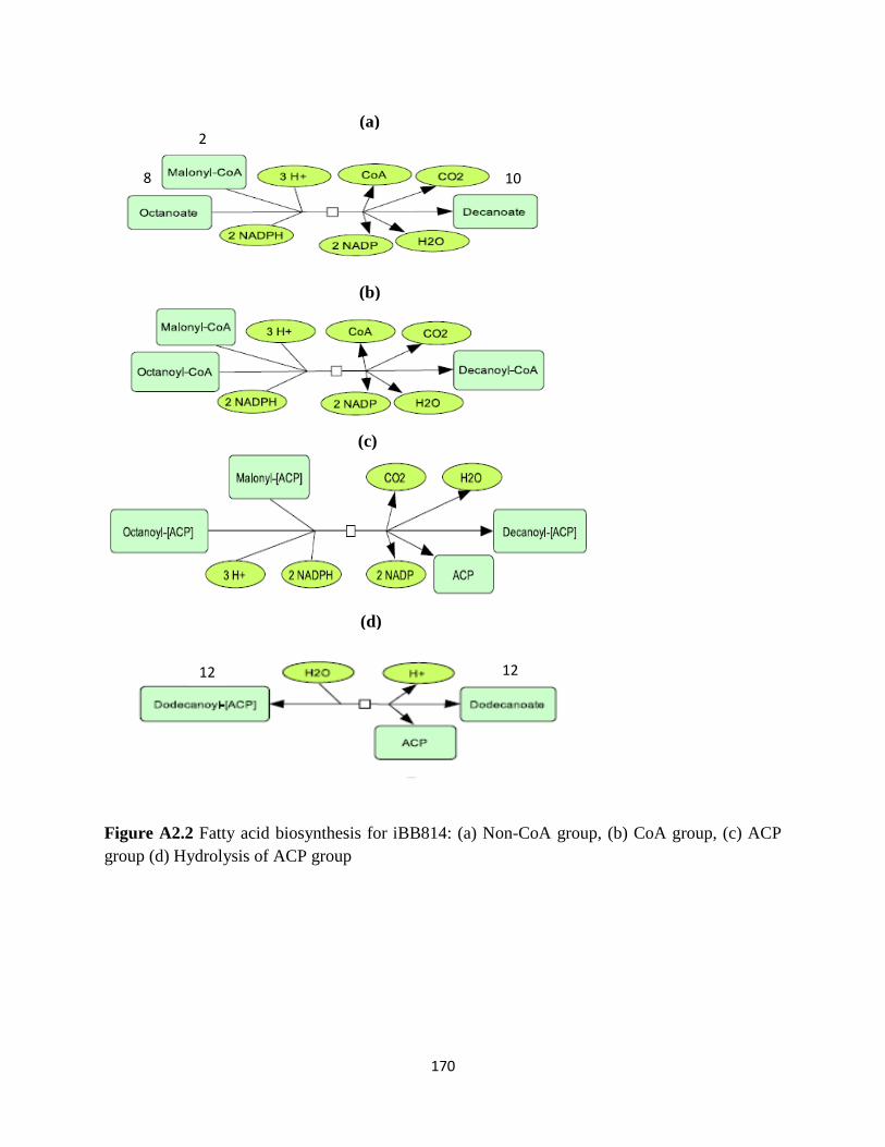
170

Figure A2.2 Fatty acid biosynthesis for iBB814: (a) Non-CoA group, (b) CoA group, (c) ACP

group (d) Hydrolysis of ACP group

8

2

10

12 12

(a)

(b)

(c)

(d)

171

A3 Biomass Composition

Amino acids

Amino Acid iSS884 iBB814 Amino Acid iSS884 iBB814

ala-L[c] 0.496 0.4735 lys-L[c] 0.200 0.2624

arg-L[c] 0.1783 0.1821 met-L[c] 0.1577 0.0559

asn-L[c] 0.0719 0.1511 L-orn[c] 0.0258 Not Present

asp-L[c] 0.100 0.1566 phe-L[c] 0.0315 0.1147

cys-L[c] 0.0415 0.0511 pro-L[c] 0.141 0.1592

gln-L[c] 0.447 0.1817 ser-L[c] 0.1359 0.2330

glu-L[c] 0.447 0.3190 thr-L[c] 0.128 0.1809

gly[c] 0.186 0.4724 trp-L[c] 0.0483 0.0248

his-L[c] 0.143 0.1005 tyr-L[c] 0.033 0.0741

ile-L[c] 0.138 0.1454 val-L[c] 0.166 0.2201

leu-L[c] 0.0799 0.251

Carbohydrates

Carbohydrates iSS884 iBB814

13BDglcn[c] 1.798 0.6107

chitin[c] Not Present 0.4528

glycogen[c] 0.178 0.2714

mannan[c] Not Present 0.7156

tre[c] 0.0102 0.076

Fatty Acids

Fatty Acids iSS884 iBB814 Fatty Acids iSS884 iBB814

clpn[c] 0.002 Not Present pe[c] 0.064 4.1 x 10-5

eig3p[c] 0.0007 Not Present ps[c] 0.001 Not Present

ergst[c] 0.0388 0.0560 ptd1ino[c] 0.003 1.5 x 10-5

fecost[c] 0.0007 Not Present 9ZHexdece[c] 0.0043 Not Present

hdca[c] 0.0119 Not Present 9ZOctadece[c] 0.0199 Not Present

lanost[c] 0.0002 Not Present 9Z12ZOctadecad[c] 0.0218 Not Present

ocdca[c] 0.0029 Not Present (9Z,12Z,15Z)-Ocdeat[c] 0.0179 Not Present

pa[c] 0.001 Not Present (9Z,12Z,15Z)-Ocdeat[c] 0.0179 Not Present

pc[c] 2.55 x 10-3

zymst[c] 0.002 Not Present

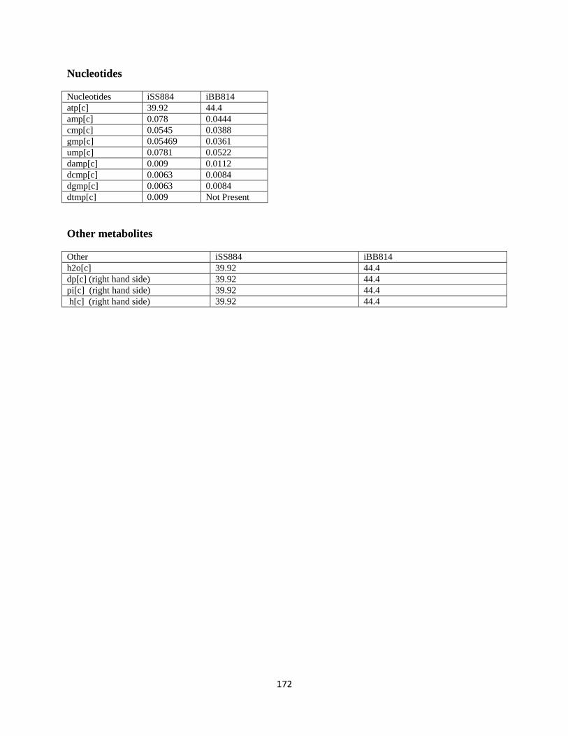
172

Nucleotides

Nucleotides iSS884 iBB814

atp[c] 39.92 44.4

amp[c] 0.078 0.0444

cmp[c] 0.0545 0.0388

gmp[c] 0.05469 0.0361

ump[c] 0.0781 0.0522

damp[c] 0.009 0.0112

dcmp[c] 0.0063 0.0084

dgmp[c] 0.0063 0.0084

dtmp[c] 0.009 Not Present

Other metabolites

Other iSS884 iBB814

h2o[c] 39.92 44.4

dp[c] (right hand side) 39.92 44.4

pi[c] (right hand side) 39.92 44.4

h[c] (right hand side) 39.92 44.4

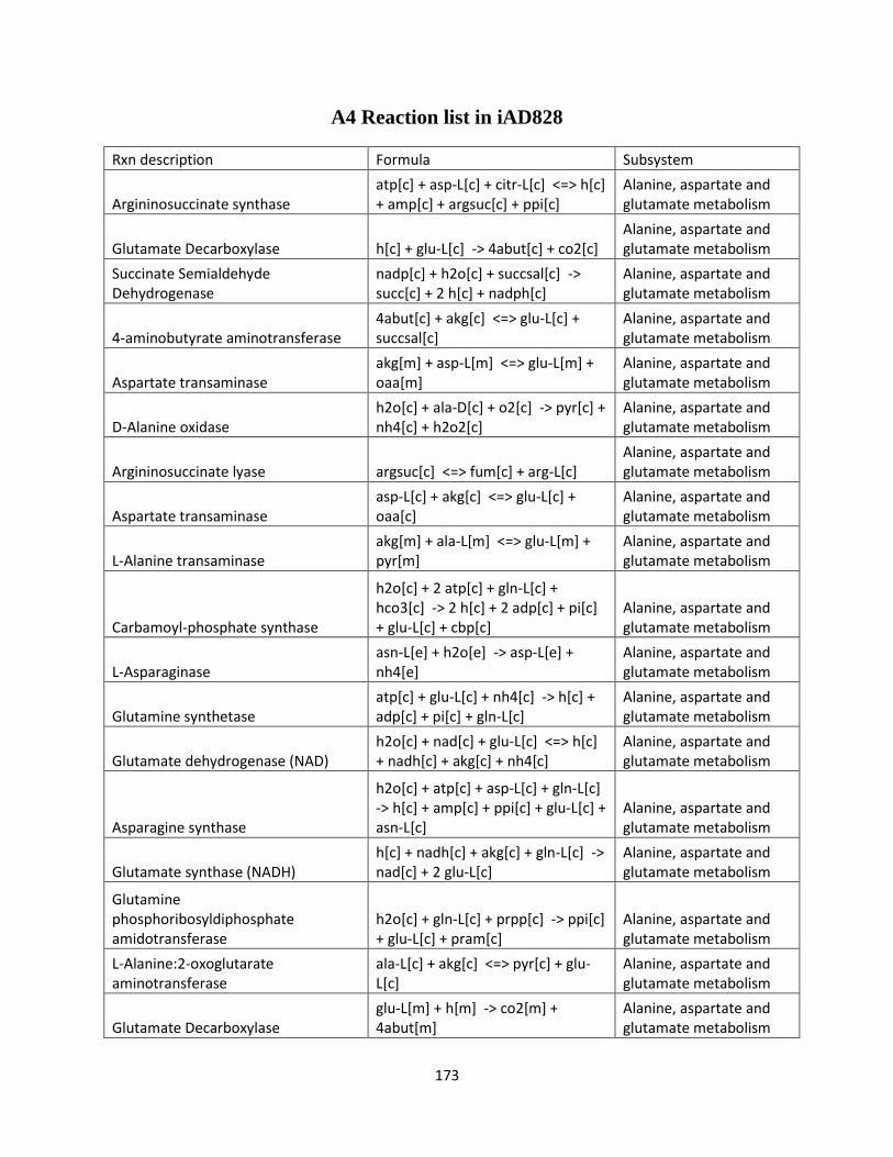
173

A4 Reaction list in iAD828

Rxn description Formula Subsystem

Argininosuccinate synthase atp[c] + asp-L[c] + citr-L[c] <=> h[c] + amp[c] + argsuc[c] + ppi[c]

Alanine, aspartate and glutamate metabolism

Glutamate Decarboxylase h[c] + glu-L[c] -> 4abut[c] + co2[c] Alanine, aspartate and glutamate metabolism

Succinate Semialdehyde Dehydrogenase

nadp[c] + h2o[c] + succsal[c] -> succ[c] + 2 h[c] + nadph[c]

Alanine, aspartate and glutamate metabolism

4-aminobutyrate aminotransferase 4abut[c] + akg[c] <=> glu-L[c] + succsal[c]

Alanine, aspartate and glutamate metabolism

Aspartate transaminase akg[m] + asp-L[m] <=> glu-L[m] + oaa[m]

Alanine, aspartate and glutamate metabolism

D-Alanine oxidase h2o[c] + ala-D[c] + o2[c] -> pyr[c] + nh4[c] + h2o2[c]

Alanine, aspartate and glutamate metabolism

Argininosuccinate lyase argsuc[c] <=> fum[c] + arg-L[c] Alanine, aspartate and glutamate metabolism

Aspartate transaminase asp-L[c] + akg[c] <=> glu-L[c] + oaa[c]

Alanine, aspartate and glutamate metabolism

L-Alanine transaminase akg[m] + ala-L[m] <=> glu-L[m] + pyr[m]

Alanine, aspartate and glutamate metabolism

Carbamoyl-phosphate synthase

h2o[c] + 2 atp[c] + gln-L[c] + hco3[c] -> 2 h[c] + 2 adp[c] + pi[c] + glu-L[c] + cbp[c]

Alanine, aspartate and glutamate metabolism

L-Asparaginase asn-L[e] + h2o[e] -> asp-L[e] + nh4[e]

Alanine, aspartate and glutamate metabolism

Glutamine synthetase atp[c] + glu-L[c] + nh4[c] -> h[c] + adp[c] + pi[c] + gln-L[c]

Alanine, aspartate and glutamate metabolism

Glutamate dehydrogenase (NAD) h2o[c] + nad[c] + glu-L[c] <=> h[c] + nadh[c] + akg[c] + nh4[c]

Alanine, aspartate and glutamate metabolism

Asparagine synthase

h2o[c] + atp[c] + asp-L[c] + gln-L[c] -> h[c] + amp[c] + ppi[c] + glu-L[c] + asn-L[c]

Alanine, aspartate and glutamate metabolism

Glutamate synthase (NADH) h[c] + nadh[c] + akg[c] + gln-L[c] -> nad[c] + 2 glu-L[c]

Alanine, aspartate and glutamate metabolism

Glutamine phosphoribosyldiphosphate amidotransferase

h2o[c] + gln-L[c] + prpp[c] -> ppi[c] + glu-L[c] + pram[c]

Alanine, aspartate and glutamate metabolism

L-Alanine:2-oxoglutarate aminotransferase

ala-L[c] + akg[c] <=> pyr[c] + glu-L[c]

Alanine, aspartate and glutamate metabolism

Glutamate Decarboxylase glu-L[m] + h[m] -> co2[m] + 4abut[m]

Alanine, aspartate and glutamate metabolism

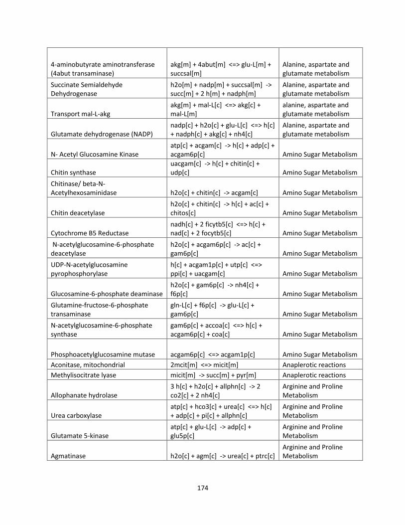
174

4-aminobutyrate aminotransferase (4abut transaminase)

akg[m] + 4abut[m] <=> glu-L[m] + succsal[m]

Alanine, aspartate and glutamate metabolism

Succinate Semialdehyde Dehydrogenase

h2o[m] + nadp[m] + succsal[m] -> succ[m] + 2 h[m] + nadph[m]

Alanine, aspartate and glutamate metabolism

Transport mal-L-akg akg[m] + mal-L[c] <=> akg[c] + mal-L[m]

alanine, aspartate and glutamate metabolism

Glutamate dehydrogenase (NADP) nadp[c] + h2o[c] + glu-L[c] <=> h[c] + nadph[c] + akg[c] + nh4[c]

Alanine, aspartate and glutamate metabolism

N- Acetyl Glucosamine Kinase atp[c] + acgam[c] -> h[c] + adp[c] + acgam6p[c] Amino Sugar Metabolism

Chitin synthase uacgam[c] -> h[c] + chitin[c] + udp[c] Amino Sugar Metabolism

Chitinase/ beta-N-Acetylhexosaminidase h2o[c] + chitin[c] -> acgam[c] Amino Sugar Metabolism

Chitin deacetylase h2o[c] + chitin[c] -> h[c] + ac[c] + chitos[c] Amino Sugar Metabolism

Cytochrome B5 Reductase nadh[c] + 2 ficytb5[c] <=> h[c] + nad[c] + 2 focytb5[c] Amino Sugar Metabolism

N-acetylglucosamine-6-phosphate deacetylase

h2o[c] + acgam6p[c] -> ac[c] + gam6p[c] Amino Sugar Metabolism

UDP-N-acetylglucosamine pyrophosphorylase

h[c] + acgam1p[c] + utp[c] <=> ppi[c] + uacgam[c] Amino Sugar Metabolism

Glucosamine-6-phosphate deaminase h2o[c] + gam6p[c] -> nh4[c] + f6p[c] Amino Sugar Metabolism

Glutamine-fructose-6-phosphate transaminase

gln-L[c] + f6p[c] -> glu-L[c] + gam6p[c] Amino Sugar Metabolism

N-acetylglucosamine-6-phosphate synthase

gam6p[c] + accoa[c] <=> h[c] + acgam6p[c] + coa[c] Amino Sugar Metabolism

Phosphoacetylglucosamine mutase acgam6p[c] <=> acgam1p[c] Amino Sugar Metabolism

Aconitase, mitochondrial 2mcit[m] <=> micit[m] Anaplerotic reactions

Methylisocitrate lyase micit[m] -> succ[m] + pyr[m] Anaplerotic reactions

Allophanate hydrolase 3 h[c] + h2o[c] + allphn[c] -> 2 co2[c] + 2 nh4[c]

Arginine and Proline Metabolism

Urea carboxylase atp[c] + hco3[c] + urea[c] <=> h[c] + adp[c] + pi[c] + allphn[c]

Arginine and Proline Metabolism

Glutamate 5-kinase atp[c] + glu-L[c] -> adp[c] + glu5p[c]

Arginine and Proline Metabolism

Agmatinase h2o[c] + agm[c] -> urea[c] + ptrc[c] Arginine and Proline Metabolism

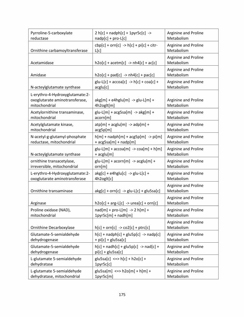
175

Pyrroline-5-carboxylate reductase

2 h[c] + nadph[c] + 1pyr5c[c] -> nadp[c] + pro-L[c]

Arginine and Proline Metabolism

Ornithine carbamoyltransferase cbp[c] + orn[c] -> h[c] + pi[c] + citr-L[c]

Arginine and Proline Metabolism

Acetamidase h2o[c] + acetm[c] -> nh4[c] + ac[c] Arginine and Proline Metabolism

Amidase h2o[c] + pad[c] -> nh4[c] + pac[c] Arginine and Proline Metabolism

N-acteylglutamate synthase glu-L[c] + accoa[c] -> h[c] + coa[c] + acglu[c]

Arginine and Proline Metabolism

L-erythro-4-Hydroxyglutamate:2-oxoglutarate aminotransferase, mitochondrial

akg[m] + e4hglu[m] -> glu-L[m] + 4h2oglt[m]

Arginine and Proline Metabolism

Acetylornithine transaminase, mitochondrial

glu-L[m] + acg5sa[m] -> akg[m] + acorn[m]

Arginine and Proline Metabolism

Acetylglutamate kinase, mitochondrial

atp[m] + acglu[m] -> adp[m] + acg5p[m]

Arginine and Proline Metabolism

N-acetyl-g-glutamyl-phosphate reductase, mitochondrial

h[m] + nadph[m] + acg5p[m] -> pi[m] + acg5sa[m] + nadp[m]

Arginine and Proline Metabolism

N-acteylglutamate synthase glu-L[m] + accoa[m] -> coa[m] + h[m] + acglu[m]

Arginine and Proline Metabolism

ornithine transacetylase, irreversible, mitochondrial

glu-L[m] + acorn[m] -> acglu[m] + orn[m]

Arginine and Proline Metabolism

L-erythro-4-Hydroxyglutamate:2-oxoglutarate aminotransferase

akg[c] + e4hglu[c] -> glu-L[c] + 4h2oglt[c]

Arginine and Proline Metabolism

Ornithine transaminase akg[c] + orn[c] -> glu-L[c] + glu5sa[c] Arginine and Proline Metabolism

Arginase h2o[c] + arg-L[c] -> urea[c] + orn[c] Arginine and Proline Metabolism

Proline oxidase (NAD), mitochondrial

nad[m] + pro-L[m] -> 2 h[m] + 1pyr5c[m] + nadh[m]

Arginine and Proline Metabolism

Ornithine Decarboxylase h[c] + orn[c] -> co2[c] + ptrc[c] Arginine and Proline Metabolism

Glutamate-5-semialdehyde dehydrogenase

h[c] + nadph[c] + glu5p[c] -> nadp[c] + pi[c] + glu5sa[c]

Arginine and Proline Metabolism

Glutamate-5-semialdehyde dehydrogenase

h[c] + nadh[c] + glu5p[c] -> nad[c] + pi[c] + glu5sa[c]

Arginine and Proline Metabolism

L-glutamate 5-semialdehyde dehydratase

glu5sa[c] <=> h[c] + h2o[c] + 1pyr5c[c]

Arginine and Proline Metabolism

L-glutamate 5-semialdehyde dehydratase, mitochondrial

glu5sa[m] <=> h2o[m] + h[m] + 1pyr5c[m]

Arginine and Proline Metabolism

176

1-Pyrroline-5-carboxylate dehydrogenase

h[c] + nadh[c] + glu-L[c] <=> 2 h2o[c] + nad[c] + 1pyr5c[c]

Arginine and Proline Metabolism

1-Pyrroline-5-carboxylate dehydrogenase

glu-L[m] + h[m] + nadh[m] <=> 2 h2o[m] + nad[m] + 1pyr5c[m]

Arginine and Proline Metabolism

Aldehyde dehydrogenase (3-aminopropanal, NAD)

h2o[c] + nad[c] + aproa[c] -> 2 h[c] + nadh[c] + ala-B[c] beta-Alanine metabolism

Aspartate 1 decarboxylase h[c] + asp-L[c] -> co2[c] + ala-B[c] beta-Alanine metabolism

Biomass Formation reaction

0.4735 ala-L[c] + 0.2201 val-L[c] + 44.4 h2o[c] + 0.1566 asp-L[c] + 0.0444 amp[c] + 0.319 glu-L[c] + 0.1821 arg-L[c] + 0.1817 gln-L[c] + 0.1511 asn-L[c] + 0.4528 chitin[c] + 0.1592 pro-L[c] + 0.0559 met-L[c] + 0.0511 cys-L[c] + 0.233 ser-L[c] + 0.4724 gly[c] + 0.1005 his-L[c] + 0.1809 thr-L[c] + 0.7156 mannan[c] + 0.000255 pc[c] + 4.1e-05 pe[c] + 0.0388 cmp[c] + 1.5e-05 ptd1ino[c] + 0.2624 lys-L[c] + 0.0361 gmp[c] + 0.0112 dtmp[c] + 0.0741 tyr-L[c] + 0.1147 phe-L[c] + 0.0248 trp-L[c] + 0.0522 ump[c] + 0.0084 dcmp[c] + 0.0112 damp[c] + 0.0084 dgmp[c] + 0.056 ergst[c] + 0.0022 zymst[c] + 0.2714 glycogen[c] + 0.6107 13BDglcn[c] + 0.076 tre[c] + 0.1454 ile-L[c] + 0.2451 leu-L[c] -> .00001 h[c] Biomass

Biotin synthase dtbt[c] + s[c] <=> 2 h[c] + btn[c] Biotin Metabolism

Adenosylmethionine-8-amino-7-oxononanoate transaminase

8aonn[c] + amet[c] <=> amob[c] + dann[c] Biotin Metabolism

Dethiobiotin synthase atp[c] + co2[c] + dann[c] <=> 3 h[c] + adp[c] + pi[c] + dtbt[c] Biotin Metabolism

(R,R)-butanediol dehydrogenase nad[c] + btd-RR[c] <=> h[c] + nadh[c] + actn-R[c] Butanoate Metabolism

Succinate-CoA ligase (ATP-forming)

adp[m] + pi[m] + succoa[m] <=> succ[m] + atp[m] + coa[m] Citrate cycle (TCA cycle)

Succinate-CoA ligase (GDP-forming)

pi[m] + succoa[m] + gdp[m] <=> succ[m] + coa[m] + gtp[m] Citrate cycle (TCA cycle)

Succinate Dehydrogenase (Flavoprotein) Mitochondrial

succ[m] + fad[m] <=> fadh2[m] + fum[m] Citrate cycle (TCA cycle)

177

Malate dehydrogenase, mitochondrial nad[m] + mal-L[m] <=> oaa[m] + h[m] + nadh[m] Citrate cycle (TCA cycle)

Isocitrate dehydrogenase (NAD+), mitochondrial

nad[m] + icit[m] -> akg[m] + nadh[m] + co2[m] Citrate cycle (TCA cycle)

isocitrate dehydrogenase (NADP+) Mitochondrial

nadp[m] + icit[m] -> akg[m] + nadph[m] + co2[m] Citrate cycle (TCA cycle)

2-Oxoglutarate Dehydrogenase (Mitochondrial)

coa[m] + akg[m] + nad[m] -> succoa[m] + nadh[m] + co2[m] Citrate cycle (TCA cycle)

Aconitate Hydratase cit[m] <=> icit[m] Citrate cycle (TCA cycle)

Citrate Synthetase oaa[m] + h2o[m] + accoa[m] -> coa[m] + h[m] + cit[m] Citrate cycle (TCA cycle)

Fumarase, mitochondrial h2o[m] + fum[m] -> mal-L[m] Citrate cycle (TCA cycle)

Isocitrate dehydrogenase nad[c] + icit[c] -> nadh[c] + co2[c] + akg[c] Citrate cycle (TCA cycle)

Homocysteine S-methyltransferase amet[c] + hcys-L[c] -> h[c] + ahcys[c] + met-L[c]

Cysteine and Methionine Metabolism

O-succinylhomoserine lyase (L-cysteine) cys-L[c] + suchms[c] -> succ[c] + h[c] + cyst-L[c]

Cysteine and Methionine Metabolism

O-succinylhomoserine lyase h2o[c] + suchms[c] <=> succ[c] + h[c] + nh4[c] + 2obut[c]

Cysteine and Methionine Metabolism

2,3-diketo-5-methylthio-1-phosphopentane degradation reaction

3 h2o[c] + dkmpp[c] -> 6 h[c] + pi[c] + 2kmb[c] + for[c]

Cysteine and Methionine Metabolism

3-Sulfo-L-alanine carboxy-lyase lcyst[c] -> co2[c] + taur[c] Cysteine and Methionine Metabolism

5-Methylthio-5-deoxy-D-ribulose 1-phosphate dehydratase 5mdru1p[c] -> h2o[c] + dkmpp[c]

Cysteine and Methionine Metabolism

Homoserine dehydrogenase (NAD) h[c] + nadh[c] + aspsa[c] -> nad[c] + hom-L[c]

Cysteine and methionine metabolism

Methionine adenosyltransferase h2o[c] + atp[c] + met-L[c] -> pi[c] + ppi[c] + amet[c]

Cysteine and Methionine Metabolism

5'-methylthioadenosine phosphorylase pi[c] + 5mta[c] -> 5mdr1p[c] + ade[c]

Cysteine and Methionine Metabolism

2-keto-4-methylthiobutyrate transamination

glu-L[c] + 2kmb[c] -> akg[c] + met-L[c]

Cysteine and Methionine Metabolism

Aspartate kinase atp[c] + asp-L[c] -> adp[c] + 4pasp[c]

Cysteine and methionine metabolism

Adenosylhomocysteinase h2o[c] + ahcys[c] -> hcys-L[c] + adn[c]

Cysteine and Methionine Metabolism

Methionine synthase hcys-L[c] + 5mthf[c] -> met-L[c] + thf[c]

Cysteine and Methionine Metabolism

178

5-methyltetrahydropteroyltriglutamate-homocysteine S-methyltransferase

hcys-L[c] + mhpglu[c] -> met-L[c] + hpglu[c]

Cysteine and Methionine Metabolism

Spermidine synthase ptrc[c] + ametam[c] -> h[c] + 5mta[c] + spmd[c]

Cysteine and methionine metabolism

Spermine synthase ametam[c] + spmd[c] -> h[c] + 5mta[c] + sprm[c]

Cysteine and methionine metabolism

Adenosylmethionine decarboxylase h[c] + amet[c] -> co2[c] + ametam[c]

Cysteine and methionine metabolism

Aspartate-semialdehyde dehydrogenase

h[c] + nadph[c] + 4pasp[c] -> nadp[c] + pi[c] + aspsa[c]

Cysteine and methionine metabolism

5-methylthioribose-1-phosphate isomerase 5mdr1p[c] <=> 5mdru1p[c]

Cysteine and Methionine Metabolism

Serine O-acetyltransferase, irreversible

accoa[c] + ser-L[c] -> coa[c] + acser[c]

Cysteine and Methionine Metabolism

Cysteine synthase acser[c] + h2s[c] -> h[c] + ac[c] + cys-L[c]

Cysteine and methionine metabolism

Homoserine O-trans-acetylase accoa[c] + hom-L[c] <=> coa[c] + achms[c]

Cysteine and methionine metabolism

O-acetylhomoserine (thiol)-lyase achms[c] + ch4s[c] -> h[c] + ac[c] + met-L[c]

Cysteine and methionine metabolism

Cystathionine b-lyase h2o[c] + cyst-L[c] -> pyr[c] + nh4[c] + hcys-L[c]

Cysteine and methionine metabolism

Cystathionine g-lyase h2o[c] + cyst-L[c] -> nh4[c] + cys-L[c] + 2obut[c]

Cysteine and methionine metabolism

Non-Specific Peptidase h2o[c] + alaasp[c] -> ala-L[c] + asp-L[c] Dipeptide metabolism

Non-Specific Peptidase h2o[c] + glyglu[c] -> glu-L[c] + gly[c] Dipeptide metabolism

Non-Specific Peptidase h2o[c] + glymet[c] -> met-L[c] + gly[c] Dipeptide metabolism

Non-Specific Peptidase h2o[c] + metala[c] -> ala-L[c] + met-L[c] Dipeptide metabolism

Non-Specific Peptidase h2o[c] + glyasp[c] -> asp-L[c] + gly[c] Dipeptide metabolism

Non-Specific Peptidase h2o[c] + glypro[c] -> pro-L[c] + gly[c] Dipeptide metabolism

Non-Specific Peptidase h2o[c] + gluala[c] -> ala-L[c] + glu-L[c] Dipeptide metabolism

Non-Specific Peptidase h2o[c] + alagln[c] -> ala-L[c] + gln-L[c] Dipeptide metabolism

179

Non-Specific Peptidase h2o[c] + alaglu[c] -> ala-L[c] + glu-L[c] Dipeptide metabolism

Non-Specific Peptidase h2o[c] + alagly[c] -> ala-L[c] + gly[c] Dipeptide metabolism

Non-Specific Peptidase h2o[c] + alahis[c] -> ala-L[c] + his-L[c] Dipeptide metabolism

Non-Specific Peptidase alaleu[c] -> ala-L[c] + h2o[c] Dipeptide metabolism

Non-Specific Peptidase h2o[c] + alathr[c] -> ala-L[c] + thr-L[c] Dipeptide metabolism

Non-Specific Peptidase h2o[c] + glyasn[c] -> asn-L[c] + gly[c] Dipeptide metabolism

Non-Specific Peptidase h2o[c] + glygln[c] -> gln-L[c] + gly[c] Dipeptide metabolism

1,3-beta-D-Glucan exchange 13BDglcn[e] <=> Exchange Reaction

2-methylbutyraldehyde exchange 2mbald[e] <=> Exchange Reaction

2-methyl-1-butanol exchange 2mbtoh[e] <=> Exchange Reaction

2-methylpropanal exchange 2mppal[e] <=> Exchange Reaction

2-oxobutanoate exchange 2obut[e] -> Exchange Reaction

2-Phosphoglycerate Exchange 2pg[e] <=> Exchange Reaction

2-Phosphoglycolate Exchange 2pglyc[e] <=> Exchange Reaction

2-phenylethanol exchange 2phetoh[e] <=> Exchange Reaction

3-Carboxy-3-hydroxy-4-methylpentanoate exchange 3c3hmp[e] <=> Exchange Reaction

3-Methylbutanal exchange 3mbald[e] <=> Exchange Reaction

3-Methyl-2-oxopentanoate exchange 3mop[e] <=> Exchange Reaction

3-Phosphoglycerate Exchange 3pg[e] <=> Exchange Reaction

4-Aminobutanoate exchange 4abut[e] <=> Exchange Reaction

4-Aminobenzoate exchange 4abz[e] <=> Exchange Reaction

hydroxyproline exchange 4hpro-LT[e] -> Exchange Reaction

5-Amino-4-oxopentanoate exchange 5aop[e] <=> Exchange Reaction

6-Phospho Gluconate Exchange 6pgc[e] <=> Exchange Reaction

8-Amino-7-oxononanoate exchange 8aonn[e] <=> Exchange Reaction

Acetate exchange ac[e] <=> Exchange Reaction

Acetoacetate exchange acac[e] -> Exchange Reaction

Acetaldehyde exchange acald[e] <=> Exchange Reaction

Acetamide exchange acetm[e] -> Exchange Reaction

Adenine exchange ade[e] <=> Exchange Reaction

Adenosine exchange adn[e] <=> Exchange Reaction

Agmatine exchange agm[e] -> Exchange Reaction

2-Oxoglutarate exchange akg[e] <=> Exchange Reaction

Ala-Asp Exchange alaasp[e] -> Exchange Reaction

D-Alanine exchange ala-D[e] -> Exchange Reaction

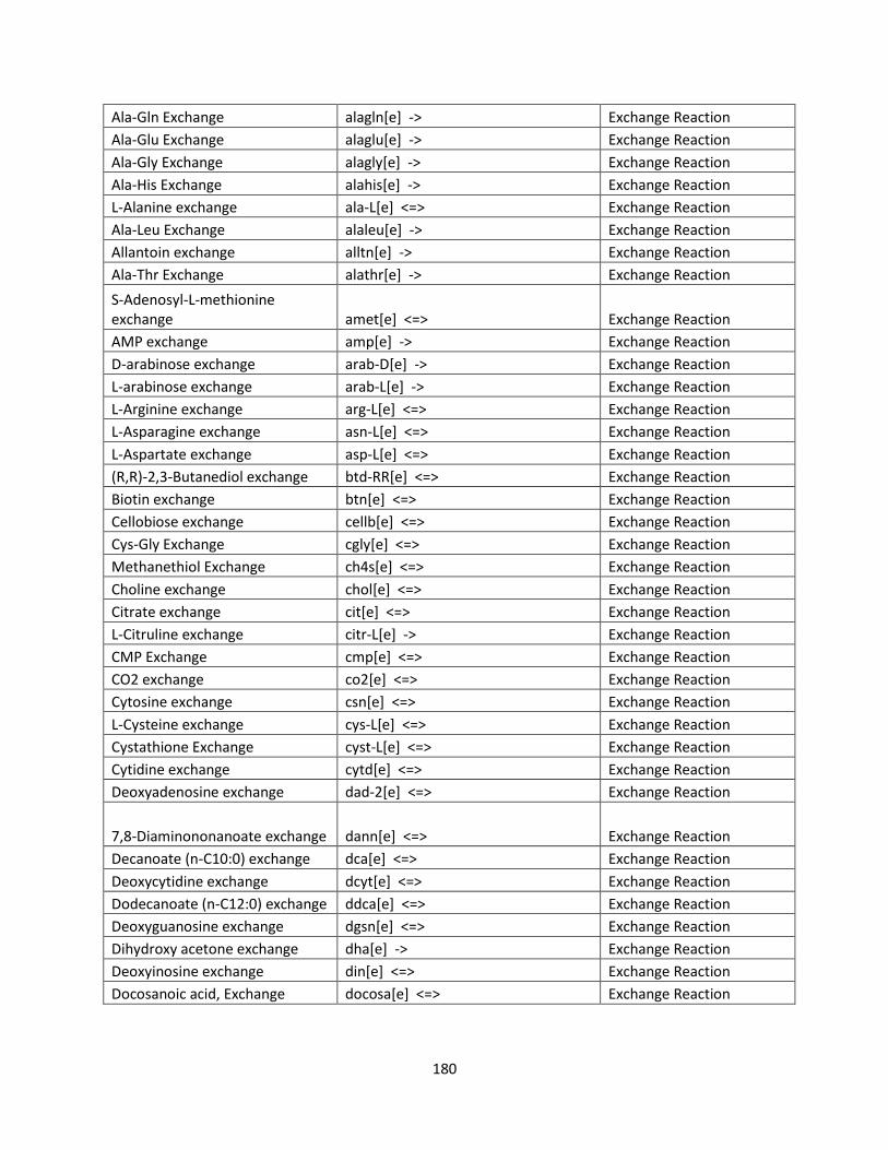
180

Ala-Gln Exchange alagln[e] -> Exchange Reaction

Ala-Glu Exchange alaglu[e] -> Exchange Reaction

Ala-Gly Exchange alagly[e] -> Exchange Reaction

Ala-His Exchange alahis[e] -> Exchange Reaction

L-Alanine exchange ala-L[e] <=> Exchange Reaction

Ala-Leu Exchange alaleu[e] -> Exchange Reaction

Allantoin exchange alltn[e] -> Exchange Reaction

Ala-Thr Exchange alathr[e] -> Exchange Reaction

S-Adenosyl-L-methionine exchange amet[e] <=> Exchange Reaction

AMP exchange amp[e] -> Exchange Reaction

D-arabinose exchange arab-D[e] -> Exchange Reaction

L-arabinose exchange arab-L[e] -> Exchange Reaction

L-Arginine exchange arg-L[e] <=> Exchange Reaction

L-Asparagine exchange asn-L[e] <=> Exchange Reaction

L-Aspartate exchange asp-L[e] <=> Exchange Reaction

(R,R)-2,3-Butanediol exchange btd-RR[e] <=> Exchange Reaction

Biotin exchange btn[e] <=> Exchange Reaction

Cellobiose exchange cellb[e] <=> Exchange Reaction

Cys-Gly Exchange cgly[e] <=> Exchange Reaction

Methanethiol Exchange ch4s[e] <=> Exchange Reaction

Choline exchange chol[e] <=> Exchange Reaction

Citrate exchange cit[e] <=> Exchange Reaction

L-Citruline exchange citr-L[e] -> Exchange Reaction

CMP Exchange cmp[e] <=> Exchange Reaction

CO2 exchange co2[e] <=> Exchange Reaction

Cytosine exchange csn[e] <=> Exchange Reaction

L-Cysteine exchange cys-L[e] <=> Exchange Reaction

Cystathione Exchange cyst-L[e] <=> Exchange Reaction

Cytidine exchange cytd[e] <=> Exchange Reaction

Deoxyadenosine exchange dad-2[e] <=> Exchange Reaction

7,8-Diaminononanoate exchange dann[e] <=> Exchange Reaction

Decanoate (n-C10:0) exchange dca[e] <=> Exchange Reaction

Deoxycytidine exchange dcyt[e] <=> Exchange Reaction

Dodecanoate (n-C12:0) exchange ddca[e] <=> Exchange Reaction

Deoxyguanosine exchange dgsn[e] <=> Exchange Reaction

Dihydroxy acetone exchange dha[e] -> Exchange Reaction

Deoxyinosine exchange din[e] <=> Exchange Reaction

Docosanoic acid, Exchange docosa[e] <=> Exchange Reaction

181

Thymidine 5 Phosphate Exchange dtmp[e] <=> Exchange Reaction

dTTP exchange dttp[e] <=> Exchange Reaction

Deoxyuridine exchange duri[e] <=> Exchange Reaction

Eicosapentaenoate, Exchange eicosapen[e] <=> Exchange Reaction

Episterol exchange epist[e] <=> Exchange Reaction

Ergosterol exchange ergst[e] <=> Exchange Reaction

Ethanolamine exchange etha[e] <=> Exchange Reaction

Ethanol exchange etoh[e] <=> Exchange Reaction

F6P exchange f6p[e] -> Exchange Reaction

Fe2+ exchange fe2[e] <=> Exchange Reaction

fecosterol exchange fecost[e] <=> Exchange Reaction

FMN exchange fmn[e] <=> Exchange Reaction

Formate exchange for[e] <=> Exchange Reaction

Formamide exchange frmd[e] -> Exchange Reaction

D-Fructose exchange fru[e] <=> Exchange Reaction

Fumarate exchange fum[e] <=> Exchange Reaction

G1P exchange g1p[e] -> Exchange Reaction

sn-Glycero-3-phosphocholine exchange g3pc[e] <=> Exchange Reaction

sn-Glycero-3-phospho-1-inositol exchange g3pi[e] <=> Exchange Reaction

G6P Exchange g6p[e] -> Exchange Reaction

D-Galactose exchange gal[e] <=> Exchange Reaction

D-Glucosamine 6-phosphate exchange gam6p[e] <=> Exchange Reaction

Glycolaldehyde exchange gcald[e] <=> Exchange Reaction

D-Glucose exchange glc-D[e] <=> Exchange Reaction

Gluconate exchange glcn-D[e] -> Exchange Reaction

L-Glutamine exchange gln-L[e] <=> Exchange Reaction

Glu-Ala Exchange gluala[e] <=> Exchange Reaction

L-Glutamate exchange glu-L[e] <=> Exchange Reaction

Glyoxylate exchange glx[e] <=> Exchange Reaction

Glycine exchange gly[e] <=> Exchange Reaction

Gly-Asn Exchange glyasn[e] -> Exchange Reaction

Gly-Asp Exchange glyasp[e] -> Exchange Reaction

Glycerol exchange glyc[e] <=> Exchange Reaction

Glycerol-3-Phosphate exchange glyc3p[e] <=> Exchange Reaction

Glycolate Exchange glyclt[e] <=> Exchange Reaction

Gly-Gln Exchange glygln[e] -> Exchange Reaction

Gly-Glu Exchange glyglu[e] -> Exchange Reaction

182

Gly-Met Exchange glymet[e] -> Exchange Reaction

Gly-Pro Exchange glypro[e] -> Exchange Reaction

GMP Exchange gmp[e] <=> Exchange Reaction

Guanosine exchange gsn[e] <=> Exchange Reaction

Oxidized glutathione exchange gthox[e] <=> Exchange Reaction

Reduced glutathione exchange gthrd[e] <=> Exchange Reaction

Guanine exchange gua[e] <=> Exchange Reaction

H+ exchange h[e] <=> Exchange Reaction

H2O exchange h2o[e] <=> Exchange Reaction

Hexadecanoate (n-C16:0) exchange hdca[e] <=> Exchange Reaction

hexadecenoate (n-C16:1) exchange hdcea[e] <=> Exchange Reaction

Heptadecenoate, Exchange hepdcea[e] <=> Exchange Reaction

hexanoate (n-C6:0) exchange hexa[e] <=> Exchange Reaction

hexacosanoate (n-C26:0) exchange hexc[e] <=> Exchange Reaction

L-Histidine exchange his-L[e] <=> Exchange Reaction

Homoserine exchange hom-L[e] -> Exchange Reaction

Isoamyl alcohol exchange iamoh[e] <=> Exchange Reaction

Isobutyl alcohol exchange ibutoh[e] <=> Exchange Reaction

L-Isoleucine exchange ile-L[e] <=> Exchange Reaction

Tryptophol Exchange ind3eth[e] -> Exchange Reaction

Myo-Inositol exchange inost[e] <=> Exchange Reaction

Inosine exchange ins[e] <=> Exchange Reaction

K+ exchange k[e] <=> Exchange Reaction

D-lactate exchange lac-D[e] <=> Exchange Reaction

L-Lactate exchange lac-L[e] <=> Exchange Reaction

Lanosterol exchange lanost[e] <=> Exchange Reaction

L-cysteate exchange lcyst[e] <=> Exchange Reaction

L-Leucine exchange leu-L[e] <=> Exchange Reaction

L-Lysine exchange lys-L[e] <=> Exchange Reaction

Alpha Methylglucoside exchange madg[e] -> Exchange Reaction

L-Malate exchange mal-L[e] <=> Exchange Reaction

Maltose exchange malt[e] <=> Exchange Reaction

Maltotriose Exchange maltr[e] -> Exchange Reaction

D-Mannose exchange man[e] <=> Exchange Reaction

Mannose 1 Phosphate Exchange man1p[e] <=> Exchange Reaction

Mannose 6 Phosphate Exchange man6p[e] <=> Exchange Reaction

D-Mannitol exchange mnl[e] -> Exchange Reaction

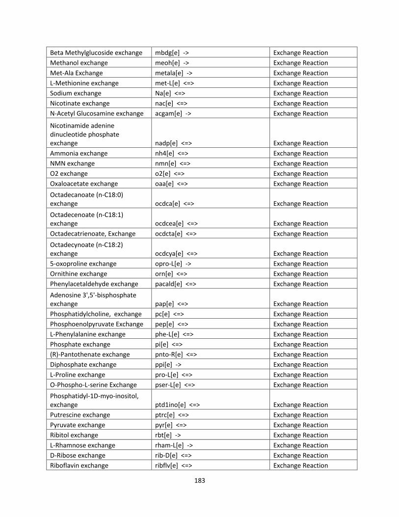
183

Beta Methylglucoside exchange mbdg[e] -> Exchange Reaction

Methanol exchange meoh[e] -> Exchange Reaction

Met-Ala Exchange metala[e] -> Exchange Reaction

L-Methionine exchange met-L[e] <=> Exchange Reaction

Sodium exchange Na[e] <=> Exchange Reaction

Nicotinate exchange nac[e] <=> Exchange Reaction

N-Acetyl Glucosamine exchange acgam[e] -> Exchange Reaction

Nicotinamide adenine dinucleotide phosphate exchange nadp[e] <=> Exchange Reaction

Ammonia exchange nh4[e] <=> Exchange Reaction

NMN exchange nmn[e] <=> Exchange Reaction

O2 exchange o2[e] <=> Exchange Reaction

Oxaloacetate exchange oaa[e] <=> Exchange Reaction

Octadecanoate (n-C18:0) exchange ocdca[e] <=> Exchange Reaction

Octadecenoate (n-C18:1) exchange ocdcea[e] <=> Exchange Reaction

Octadecatrienoate, Exchange ocdcta[e] <=> Exchange Reaction

Octadecynoate (n-C18:2) exchange ocdcya[e] <=> Exchange Reaction

5-oxoproline exchange opro-L[e] -> Exchange Reaction

Ornithine exchange orn[e] <=> Exchange Reaction

Phenylacetaldehyde exchange pacald[e] <=> Exchange Reaction

Adenosine 3',5'-bisphosphate exchange pap[e] <=> Exchange Reaction

Phosphatidylcholine, exchange pc[e] <=> Exchange Reaction

Phosphoenolpyruvate Exchange pep[e] <=> Exchange Reaction

L-Phenylalanine exchange phe-L[e] <=> Exchange Reaction

Phosphate exchange pi[e] <=> Exchange Reaction

(R)-Pantothenate exchange pnto-R[e] <=> Exchange Reaction

Diphosphate exchange ppi[e] -> Exchange Reaction

L-Proline exchange pro-L[e] <=> Exchange Reaction

O-Phospho-L-serine Exchange pser-L[e] <=> Exchange Reaction

Phosphatidyl-1D-myo-inositol, exchange ptd1ino[e] <=> Exchange Reaction

Putrescine exchange ptrc[e] <=> Exchange Reaction

Pyruvate exchange pyr[e] <=> Exchange Reaction

Ribitol exchange rbt[e] -> Exchange Reaction

L-Rhamnose exchange rham-L[e] -> Exchange Reaction

D-Ribose exchange rib-D[e] <=> Exchange Reaction

Riboflavin exchange ribflv[e] <=> Exchange Reaction

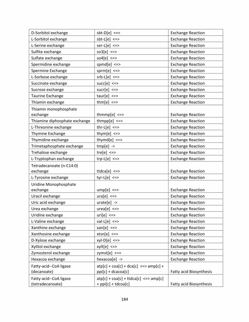
184

D-Sorbitol exchange sbt-D[e] <=> Exchange Reaction

L-Sorbitol exchange sbt-L[e] <=> Exchange Reaction

L-Serine exchange ser-L[e] <=> Exchange Reaction

Sulfite exchange so3[e] <=> Exchange Reaction

Sulfate exchange so4[e] <=> Exchange Reaction

Spermidine exchange spmd[e] <=> Exchange Reaction

Spermine Exchange sprm[e] <=> Exchange Reaction

L-Sorbose exchange srb-L[e] <=> Exchange Reaction

Succinate exchange succ[e] <=> Exchange Reaction

Sucrose exchange sucr[e] <=> Exchange Reaction

Taurine Exchange taur[e] <=> Exchange Reaction

Thiamin exchange thm[e] <=> Exchange Reaction

Thiamin monophosphate exchange thmmp[e] <=> Exchange Reaction

Thiamine diphosphate exchange thmpp[e] <=> Exchange Reaction

L-Threonine exchange thr-L[e] <=> Exchange Reaction

Thymine Exchange thym[e] <=> Exchange Reaction

Thymidine exchange thymd[e] <=> Exchange Reaction

Trimetaphosphate exchange tmp[e] -> Exchange Reaction

Trehalose exchange tre[e] <=> Exchange Reaction

L-Tryptophan exchange trp-L[e] <=> Exchange Reaction

Tetradecanoate (n-C14:0) exchange ttdca[e] <=> Exchange Reaction

L-Tyrosine exchange tyr-L[e] <=> Exchange Reaction

Uridine Monophosphate exchange ump[e] <=> Exchange Reaction

Uracil exchange ura[e] <=> Exchange Reaction

Uric acid exchange urate[e] -> Exchange Reaction

Urea exchange urea[e] <=> Exchange Reaction

Uridine exchange uri[e] <=> Exchange Reaction

L-Valine exchange val-L[e] <=> Exchange Reaction

Xanthine exchange xan[e] <=> Exchange Reaction

Xanthosine exchange xtsn[e] <=> Exchange Reaction

D-Xylose exchange xyl-D[e] <=> Exchange Reaction

Xylitol exchange xylt[e] <=> Exchange Reaction

Zymosterol exchange zymst[e] <=> Exchange Reaction

Hexacoa exchange hexacoa[e] -> Exchange Reaction

Fatty-acid--CoA ligase (decanoate)

atp[c] + coa[c] + dca[c] <=> amp[c] + ppi[c] + dcacoa[c] Fatty acid Biosynthesis

Fatty-acid--CoA ligase (tetradecanoate)

atp[c] + coa[c] + ttdca[c] <=> amp[c] + ppi[c] + tdcoa[c] Fatty acid Biosynthesis

185

Fatty-acid--CoA ligase (hexadecanoate)

atp[c] + coa[c] + hdca[c] <=> amp[c] + ppi[c] + pmtcoa[c] Fatty acid Biosynthesis

Fatty-acid--CoA ligase (hexadecenoate)

atp[c] + coa[c] + hdcea[c] <=> amp[c] + ppi[c] + hdceacoa[c] Fatty acid Biosynthesis

Fatty-acid--CoA ligase (eicosapentaenoate)

atp[c] + coa[c] + hepdca[c] <=> amp[c] + ppi[c] + hepdcacoa[c] Fatty acid Biosynthesis

Fatty-acid--CoA ligase (eicosapentaenoate)

atp[c] + coa[c] + hepdcea[c] <=> amp[c] + ppi[c] + hepdceacoa[c] Fatty acid Biosynthesis

Fatty-acid--CoA ligase (octadecanoate)

atp[c] + coa[c] + ocdca[c] <=> amp[c] + ppi[c] + stcoa[c] Fatty acid Biosynthesis

Fatty-acid--CoA ligase (octadecenoate)

atp[c] + coa[c] + ocdcea[c] <=> amp[c] + ppi[c] + ocdceacoa[c] Fatty acid Biosynthesis

Fatty-acid--CoA ligase (octadecynoate)

atp[c] + coa[c] + ocdcya[c] <=> amp[c] + ppi[c] + ocdcyacoa[c] Fatty acid Biosynthesis

Fatty-acid--CoA ligase (octadecatrieonoate)

atp[c] + coa[c] + ocdcta[c] <=> amp[c] + ppi[c] + ocdctacoa[c] Fatty acid Biosynthesis

Fatty-acid--CoA ligase (eicosapentaenoate)

atp[c] + coa[c] + eicosapen[c] <=> amp[c] + ppi[c] + eicosapencoa[c] Fatty acid Biosynthesis

Fatty-acid--CoA ligase (octanoate)

atp[c] + coa[c] + hexa[c] <=> amp[c] + ppi[c] + hexacoa[c] Fatty acid Biosynthesis

Fatty-acyl-ACP synthase (n-C10:0ACP), mitochondrial

3 h[m] + 2 nadph[m] + malACP[m] + octaACP[m] -> h2o[m] + 2 nadp[m] + co2[m] + ACP[m] + dcaACP[m] Fatty acid Biosynthesis

Fatty-acyl-ACP synthase (n-C12:0ACP), mitochondrial

3 h[m] + 2 nadph[m] + malACP[m] + dcaACP[m] -> h2o[m] + 2 nadp[m] + co2[m] + ACP[m] + ddcaACP[m] Fatty acid Biosynthesis

Fatty-acyl-ACP synthase (n-C14:0ACP), mitochondrial

3 h[m] + 2 nadph[m] + malACP[m] + ddcaACP[m] -> h2o[m] + 2 nadp[m] + co2[m] + ACP[m] + myrsACP[m] Fatty acid Biosynthesis

Fatty-acyl-ACP synthase (n-C16:0ACP), mitochondrial

3 h[m] + 2 nadph[m] + malACP[m] + myrsACP[m] -> h2o[m] + 2 nadp[m] + co2[m] + ACP[m] + palmACP[m] Fatty acid Biosynthesis

Fatty-acyl-ACP synthase (n-C16:1ACP), mitochondrial

4 h[m] + 3 nadph[m] + malACP[m] + myrsACP[m] + o2[m] -> 3 h2o[m] + 3 nadp[m] + co2[m] + ACP[m] + hdceaACP[m] Fatty acid Biosynthesis

Fatty acyl-ACP synthase (n-C17:0ACP), mitochondrial, lumped reaction

21 h[m] + 14 nadph[m] + 7 malACP[m] + ppACP[m] -> 7 h2o[m] + 14 nadp[m] + 7 co2[m] + 7 ACP[m] + hepdcaACP[m] Fatty acid Biosynthesis

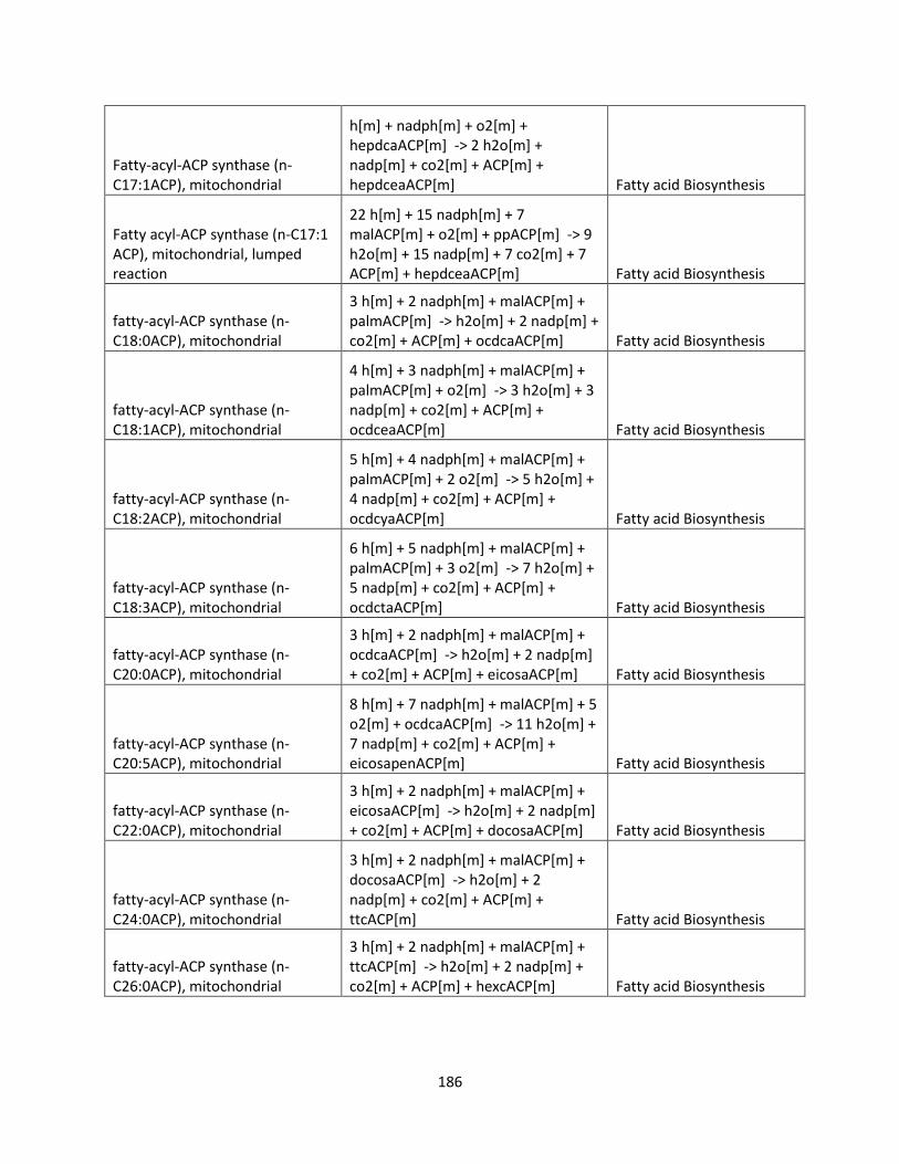
186

Fatty-acyl-ACP synthase (n-C17:1ACP), mitochondrial

h[m] + nadph[m] + o2[m] + hepdcaACP[m] -> 2 h2o[m] + nadp[m] + co2[m] + ACP[m] + hepdceaACP[m] Fatty acid Biosynthesis

Fatty acyl-ACP synthase (n-C17:1 ACP), mitochondrial, lumped reaction

22 h[m] + 15 nadph[m] + 7 malACP[m] + o2[m] + ppACP[m] -> 9 h2o[m] + 15 nadp[m] + 7 co2[m] + 7 ACP[m] + hepdceaACP[m] Fatty acid Biosynthesis

fatty-acyl-ACP synthase (n-C18:0ACP), mitochondrial

3 h[m] + 2 nadph[m] + malACP[m] + palmACP[m] -> h2o[m] + 2 nadp[m] + co2[m] + ACP[m] + ocdcaACP[m] Fatty acid Biosynthesis

fatty-acyl-ACP synthase (n-C18:1ACP), mitochondrial

4 h[m] + 3 nadph[m] + malACP[m] + palmACP[m] + o2[m] -> 3 h2o[m] + 3 nadp[m] + co2[m] + ACP[m] + ocdceaACP[m] Fatty acid Biosynthesis

fatty-acyl-ACP synthase (n-C18:2ACP), mitochondrial

5 h[m] + 4 nadph[m] + malACP[m] + palmACP[m] + 2 o2[m] -> 5 h2o[m] + 4 nadp[m] + co2[m] + ACP[m] + ocdcyaACP[m] Fatty acid Biosynthesis

fatty-acyl-ACP synthase (n-C18:3ACP), mitochondrial

6 h[m] + 5 nadph[m] + malACP[m] + palmACP[m] + 3 o2[m] -> 7 h2o[m] + 5 nadp[m] + co2[m] + ACP[m] + ocdctaACP[m] Fatty acid Biosynthesis

fatty-acyl-ACP synthase (n-C20:0ACP), mitochondrial

3 h[m] + 2 nadph[m] + malACP[m] + ocdcaACP[m] -> h2o[m] + 2 nadp[m] + co2[m] + ACP[m] + eicosaACP[m] Fatty acid Biosynthesis

fatty-acyl-ACP synthase (n-C20:5ACP), mitochondrial

8 h[m] + 7 nadph[m] + malACP[m] + 5 o2[m] + ocdcaACP[m] -> 11 h2o[m] + 7 nadp[m] + co2[m] + ACP[m] + eicosapenACP[m] Fatty acid Biosynthesis

fatty-acyl-ACP synthase (n-C22:0ACP), mitochondrial

3 h[m] + 2 nadph[m] + malACP[m] + eicosaACP[m] -> h2o[m] + 2 nadp[m] + co2[m] + ACP[m] + docosaACP[m] Fatty acid Biosynthesis

fatty-acyl-ACP synthase (n-C24:0ACP), mitochondrial

3 h[m] + 2 nadph[m] + malACP[m] + docosaACP[m] -> h2o[m] + 2 nadp[m] + co2[m] + ACP[m] + ttcACP[m] Fatty acid Biosynthesis

fatty-acyl-ACP synthase (n-C26:0ACP), mitochondrial

3 h[m] + 2 nadph[m] + malACP[m] + ttcACP[m] -> h2o[m] + 2 nadp[m] + co2[m] + ACP[m] + hexcACP[m] Fatty acid Biosynthesis

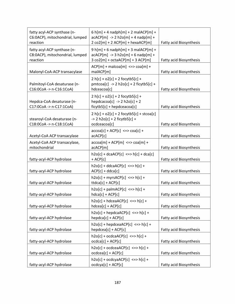
187

fatty acyl-ACP synthase (n-C6:0ACP), mitochondrial, lumped reaction

6 h[m] + 4 nadph[m] + 2 malACP[m] + acACP[m] -> 2 h2o[m] + 4 nadp[m] + 2 co2[m] + 2 ACP[m] + hexaACP[m] Fatty acid Biosynthesis

fatty acyl-ACP synthase (n-C8:0ACP), mitochondrial, lumped reaction

9 h[m] + 6 nadph[m] + 3 malACP[m] + acACP[m] -> 3 h2o[m] + 6 nadp[m] + 3 co2[m] + octaACP[m] + 3 ACP[m] Fatty acid Biosynthesis

Malonyl-CoA-ACP transacylase ACP[m] + malcoa[m] <=> coa[m] + malACP[m] Fatty acid Biosynthesis

Palmitoyl-CoA desaturase (n-C16:0CoA -> n-C16:1CoA)

2 h[c] + o2[c] + 2 focytb5[c] + pmtcoa[c] -> 2 h2o[c] + 2 ficytb5[c] + hdceacoa[c] Fatty acid Biosynthesis

Hepdca-CoA desaturase (n-C17:0CoA -> n-C17:1CoA)

2 h[c] + o2[c] + 2 focytb5[c] + hepdcacoa[c] -> 2 h2o[c] + 2 ficytb5[c] + hepdceacoa[c] Fatty acid Biosynthesis

stearoyl-CoA desaturase (n-C18:0CoA -> n-C18:1CoA)

2 h[c] + o2[c] + 2 focytb5[c] + stcoa[c] -> 2 h2o[c] + 2 ficytb5[c] + ocdceacoa[c] Fatty acid Biosynthesis

Acetyl-CoA ACP transacylase accoa[c] + ACP[c] <=> coa[c] + acACP[c] Fatty acid Biosynthesis

Acetyl-CoA ACP transacylase, mitochondrial

accoa[m] + ACP[m] <=> coa[m] + acACP[m] Fatty acid Biosynthesis

fatty-acyl-ACP hydrolase h2o[c] + dcaACP[c] <=> h[c] + dca[c] + ACP[c] Fatty acid Biosynthesis

fatty-acyl-ACP hydrolase h2o[c] + ddcaACP[c] <=> h[c] + ACP[c] + ddca[c] Fatty acid Biosynthesis

fatty-acyl-ACP hydrolase h2o[c] + myrsACP[c] <=> h[c] + ttdca[c] + ACP[c] Fatty acid Biosynthesis

fatty-acyl-ACP hydrolase h2o[c] + palmACP[c] <=> h[c] + hdca[c] + ACP[c] Fatty acid Biosynthesis

fatty-acyl-ACP hydrolase h2o[c] + hdceaACP[c] <=> h[c] + hdcea[c] + ACP[c] Fatty acid Biosynthesis

fatty-acyl-ACP hydrolase h2o[c] + hepdcaACP[c] <=> h[c] + hepdca[c] + ACP[c] Fatty acid Biosynthesis

fatty-acyl-ACP hydrolase h2o[c] + hepdceaACP[c] <=> h[c] + hepdcea[c] + ACP[c] Fatty acid Biosynthesis

fatty-acyl-ACP hydrolase h2o[c] + ocdcaACP[c] <=> h[c] + ocdca[c] + ACP[c] Fatty acid Biosynthesis

fatty-acyl-ACP hydrolase h2o[c] + ocdceaACP[c] <=> h[c] + ocdcea[c] + ACP[c] Fatty acid Biosynthesis

fatty-acyl-ACP hydrolase h2o[c] + ocdcyaACP[c] <=> h[c] + ocdcya[c] + ACP[c] Fatty acid Biosynthesis

188

fatty-acyl-ACP hydrolase h2o[c] + ocdctaACP[c] <=> h[c] + ocdcta[c] + ACP[c] Fatty acid Biosynthesis

fatty-acyl-ACP hydrolase h2o[c] + eicosaACP[c] <=> h[c] + ACP[c] + eicosa[c] Fatty acid Biosynthesis

fatty-acyl-ACP hydrolase h2o[c] + eicosapenACP[c] <=> h[c] + eicosapen[c] + ACP[c] Fatty acid Biosynthesis

fatty-acyl-ACP hydrolase h2o[c] + docosaACP[c] <=> h[c] + ACP[c] + docosa[c] Fatty acid Biosynthesis

fatty-acyl-ACP hydrolase h2o[c] + ttcACP[c] <=> h[c] + ACP[c] + ttc[c] Fatty acid Biosynthesis

fatty-acyl-ACP hydrolase h2o[c] + hexcACP[c] <=> h[c] + ACP[c] + hexc[c] Fatty acid Biosynthesis

fatty-acyl-ACP hydrolase h2o[c] + hexaACP[c] <=> h[c] + hexa[c] + ACP[c] Fatty acid Biosynthesis

fatty-acyl-ACP hydrolase h2o[c] + octaACP[c] <=> h[c] + ACP[c] + octa[c] Fatty acid Biosynthesis

fatty acid synthase (n-C10:0)

3 h[c] + 2 nadph[c] + octa[c] + malcoa[c] -> 2 nadp[c] + h2o[c] + co2[c] + coa[c] + dca[c] Fatty acid Biosynthesis

fatty acyl-CoA synthase (n-C10:0CoA)

3 h[c] + 2 nadph[c] + malcoa[c] + octacoa[c] -> 2 nadp[c] + h2o[c] + co2[c] + coa[c] + dcacoa[c] Fatty acid Biosynthesis

fatty acid synthase (n-C12:0)

3 h[c] + 2 nadph[c] + dca[c] + malcoa[c] -> 2 nadp[c] + h2o[c] + co2[c] + coa[c] + ddca[c] Fatty acid Biosynthesis

fatty-acyl-CoA synthase (n-C12:0CoA)

3 h[c] + 2 nadph[c] + dcacoa[c] + malcoa[c] -> 2 nadp[c] + h2o[c] + co2[c] + coa[c] + ddcacoa[c] Fatty acid Biosynthesis

fatty acid synthase (n-C14:0)

3 h[c] + 2 nadph[c] + ddca[c] + malcoa[c] -> 2 nadp[c] + h2o[c] + co2[c] + coa[c] + ttdca[c] Fatty acid Biosynthesis

fatty-acyl-CoA synthase (n-C14:0CoA)

3 h[c] + 2 nadph[c] + malcoa[c] + ddcacoa[c] -> 2 nadp[c] + h2o[c] + co2[c] + coa[c] + tdcoa[c] Fatty acid Biosynthesis

fatty acid synthase (n-C16:0)

3 h[c] + 2 nadph[c] + ttdca[c] + malcoa[c] -> 2 nadp[c] + h2o[c] + co2[c] + coa[c] + hdca[c] Fatty acid Biosynthesis

fatty-acyl-CoA synthase (n-C16:0CoA)

3 h[c] + 2 nadph[c] + tdcoa[c] + malcoa[c] -> 2 nadp[c] + h2o[c] + co2[c] + coa[c] + pmtcoa[c] Fatty acid Biosynthesis

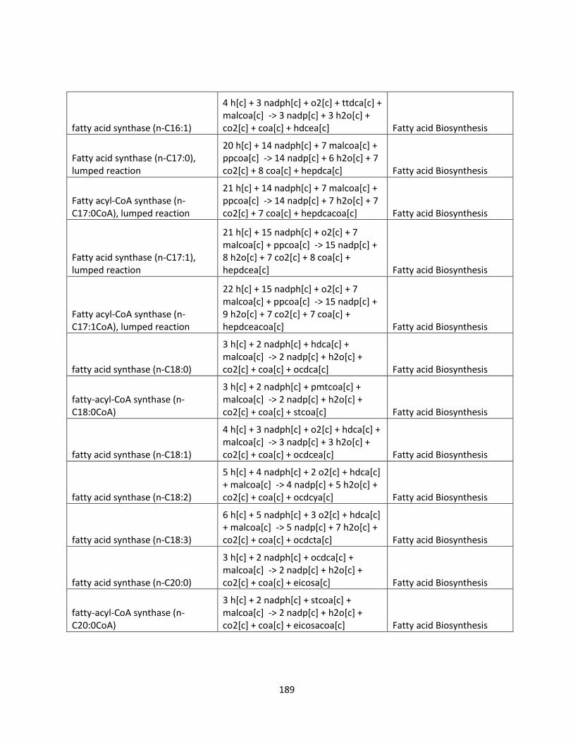
189

fatty acid synthase (n-C16:1)

4 h[c] + 3 nadph[c] + o2[c] + ttdca[c] + malcoa[c] -> 3 nadp[c] + 3 h2o[c] + co2[c] + coa[c] + hdcea[c] Fatty acid Biosynthesis

Fatty acid synthase (n-C17:0), lumped reaction

20 h[c] + 14 nadph[c] + 7 malcoa[c] + ppcoa[c] -> 14 nadp[c] + 6 h2o[c] + 7 co2[c] + 8 coa[c] + hepdca[c] Fatty acid Biosynthesis

Fatty acyl-CoA synthase (n-C17:0CoA), lumped reaction

21 h[c] + 14 nadph[c] + 7 malcoa[c] + ppcoa[c] -> 14 nadp[c] + 7 h2o[c] + 7 co2[c] + 7 coa[c] + hepdcacoa[c] Fatty acid Biosynthesis

Fatty acid synthase (n-C17:1), lumped reaction

21 h[c] + 15 nadph[c] + o2[c] + 7 malcoa[c] + ppcoa[c] -> 15 nadp[c] + 8 h2o[c] + 7 co2[c] + 8 coa[c] + hepdcea[c] Fatty acid Biosynthesis

Fatty acyl-CoA synthase (n-C17:1CoA), lumped reaction

22 h[c] + 15 nadph[c] + o2[c] + 7 malcoa[c] + ppcoa[c] -> 15 nadp[c] + 9 h2o[c] + 7 co2[c] + 7 coa[c] + hepdceacoa[c] Fatty acid Biosynthesis

fatty acid synthase (n-C18:0)

3 h[c] + 2 nadph[c] + hdca[c] + malcoa[c] -> 2 nadp[c] + h2o[c] + co2[c] + coa[c] + ocdca[c] Fatty acid Biosynthesis

fatty-acyl-CoA synthase (n-C18:0CoA)

3 h[c] + 2 nadph[c] + pmtcoa[c] + malcoa[c] -> 2 nadp[c] + h2o[c] + co2[c] + coa[c] + stcoa[c] Fatty acid Biosynthesis

fatty acid synthase (n-C18:1)

4 h[c] + 3 nadph[c] + o2[c] + hdca[c] + malcoa[c] -> 3 nadp[c] + 3 h2o[c] + co2[c] + coa[c] + ocdcea[c] Fatty acid Biosynthesis

fatty acid synthase (n-C18:2)

5 h[c] + 4 nadph[c] + 2 o2[c] + hdca[c] + malcoa[c] -> 4 nadp[c] + 5 h2o[c] + co2[c] + coa[c] + ocdcya[c] Fatty acid Biosynthesis

fatty acid synthase (n-C18:3)

6 h[c] + 5 nadph[c] + 3 o2[c] + hdca[c] + malcoa[c] -> 5 nadp[c] + 7 h2o[c] + co2[c] + coa[c] + ocdcta[c] Fatty acid Biosynthesis

fatty acid synthase (n-C20:0)

3 h[c] + 2 nadph[c] + ocdca[c] + malcoa[c] -> 2 nadp[c] + h2o[c] + co2[c] + coa[c] + eicosa[c] Fatty acid Biosynthesis

fatty-acyl-CoA synthase (n-C20:0CoA)

3 h[c] + 2 nadph[c] + stcoa[c] + malcoa[c] -> 2 nadp[c] + h2o[c] + co2[c] + coa[c] + eicosacoa[c] Fatty acid Biosynthesis

190

fatty acid synthase (n-C20:5)

8 h[c] + 7 nadph[c] + 5 o2[c] + ocdca[c] + malcoa[c] -> 7 nadp[c] + 11 h2o[c] + co2[c] + coa[c] + eicosapen[c] Fatty acid Biosynthesis

fatty acid synthase (n-C22:0)

3 h[c] + 2 nadph[c] + eicosa[c] + malcoa[c] -> 2 nadp[c] + h2o[c] + co2[c] + coa[c] + docosa[c] Fatty acid Biosynthesis

fatty-acyl-CoA synthase (n-C22:0CoA)

3 h[c] + 2 nadph[c] + malcoa[c] + eicosacoa[c] -> 2 nadp[c] + h2o[c] + co2[c] + coa[c] + docosacoa[c] Fatty acid Biosynthesis

fatty acid synthase (n-C24:0)

3 h[c] + 2 nadph[c] + docosa[c] + malcoa[c] -> 2 nadp[c] + h2o[c] + co2[c] + coa[c] + ttc[c] Fatty acid Biosynthesis

fatty-acyl-CoA synthase (n-C24:0CoA)

3 h[c] + 2 nadph[c] + malcoa[c] + docosacoa[c] -> 2 nadp[c] + h2o[c] + co2[c] + coa[c] + ttccoa[c] Fatty acid Biosynthesis

fatty acid synthase (n-C26:0)

3 h[c] + 2 nadph[c] + ttc[c] + malcoa[c] -> 2 nadp[c] + h2o[c] + co2[c] + coa[c] + hexc[c] Fatty acid Biosynthesis

fatty-acyl-CoA synthase (n-C26:0CoA)

3 h[c] + 2 nadph[c] + malcoa[c] + ttccoa[c] -> 2 nadp[c] + h2o[c] + co2[c] + coa[c] + hexccoa[c] Fatty acid Biosynthesis

Fatty acid synthase (n-C6:0), lumped reaction

5 h[c] + 4 nadph[c] + accoa[c] + 2 malcoa[c] -> 4 nadp[c] + h2o[c] + 2 co2[c] + 3 coa[c] + hexa[c] Fatty acid Biosynthesis

Fatty acyl-CoA synthase (n-C6:0CoA), lumped reaction

6 h[c] + 4 nadph[c] + accoa[c] + 2 malcoa[c] -> 4 nadp[c] + 2 h2o[c] + 2 co2[c] + 2 coa[c] + hexacoa[c] Fatty acid Biosynthesis

fatty acid synthase (n-C8:0), lumped reaction

8 h[c] + 6 nadph[c] + accoa[c] + 3 malcoa[c] -> 6 nadp[c] + 2 h2o[c] + 3 co2[c] + 4 coa[c] + octa[c] Fatty acid Biosynthesis

fatty acyl-CoA synthase (n-C8:0CoA), lumped reaction

9 h[c] + 6 nadph[c] + accoa[c] + 3 malcoa[c] -> 6 nadp[c] + 3 h2o[c] + 3 co2[c] + 3 coa[c] + octacoa[c] Fatty acid Biosynthesis

Propanoyl-CoA ACP transacylase ACP[c] + ppcoa[c] <=> coa[c] + ppACP[c] Fatty acid Biosynthesis

Propanoyl-CoA ACP transacylase, mitochondrial

ACP[m] + ppcoa[m] <=> coa[m] + ppACP[m] Fatty acid Biosynthesis

Linoeyl-CoA desaturase (n-C18:2CoA -> n-C18:2CoA)

h[c] + nadph[c] + o2[c] + ocdcyacoa[c] -> nadp[c] + 2 h2o[c] + ocdctacoa[c] Fatty acid Biosynthesis

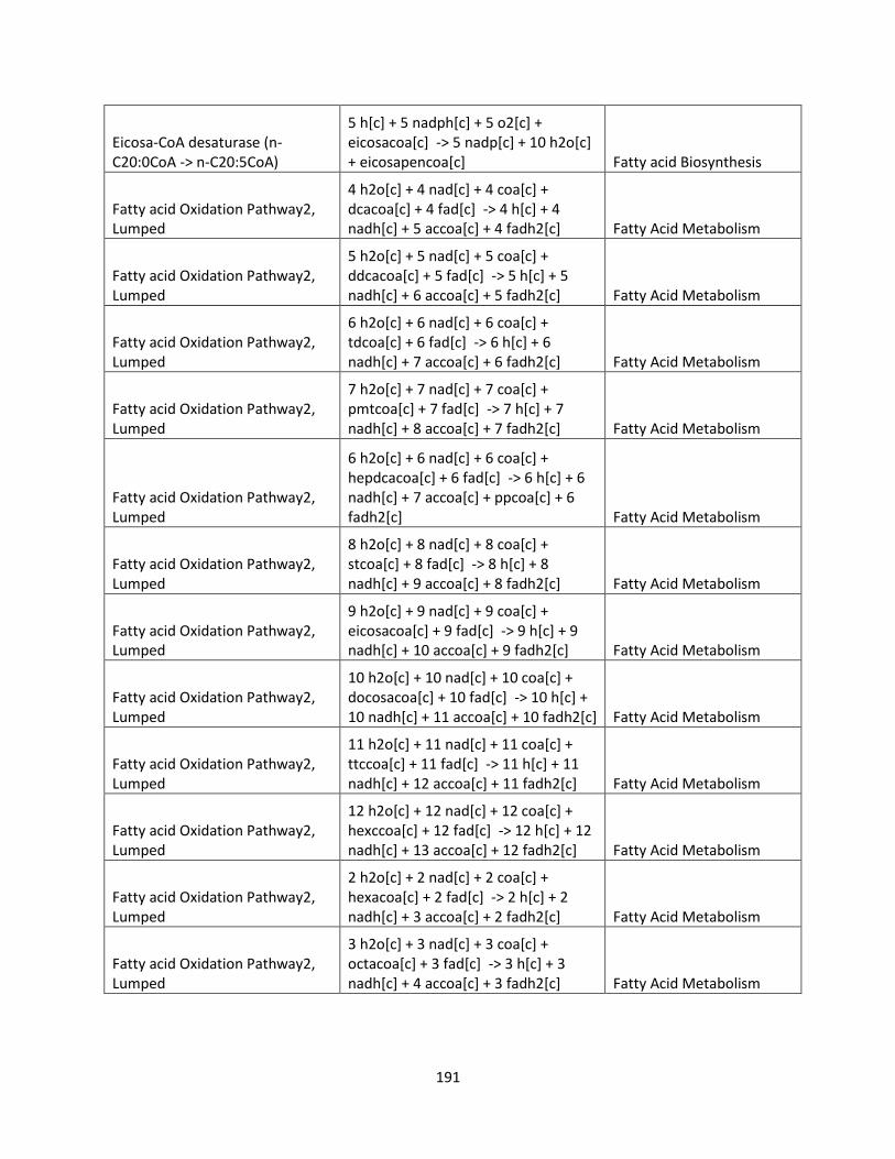
191

Eicosa-CoA desaturase (n-C20:0CoA -> n-C20:5CoA)

5 h[c] + 5 nadph[c] + 5 o2[c] + eicosacoa[c] -> 5 nadp[c] + 10 h2o[c] + eicosapencoa[c] Fatty acid Biosynthesis

Fatty acid Oxidation Pathway2, Lumped

4 h2o[c] + 4 nad[c] + 4 coa[c] + dcacoa[c] + 4 fad[c] -> 4 h[c] + 4 nadh[c] + 5 accoa[c] + 4 fadh2[c] Fatty Acid Metabolism

Fatty acid Oxidation Pathway2, Lumped

5 h2o[c] + 5 nad[c] + 5 coa[c] + ddcacoa[c] + 5 fad[c] -> 5 h[c] + 5 nadh[c] + 6 accoa[c] + 5 fadh2[c] Fatty Acid Metabolism

Fatty acid Oxidation Pathway2, Lumped

6 h2o[c] + 6 nad[c] + 6 coa[c] + tdcoa[c] + 6 fad[c] -> 6 h[c] + 6 nadh[c] + 7 accoa[c] + 6 fadh2[c] Fatty Acid Metabolism

Fatty acid Oxidation Pathway2, Lumped

7 h2o[c] + 7 nad[c] + 7 coa[c] + pmtcoa[c] + 7 fad[c] -> 7 h[c] + 7 nadh[c] + 8 accoa[c] + 7 fadh2[c] Fatty Acid Metabolism

Fatty acid Oxidation Pathway2, Lumped

6 h2o[c] + 6 nad[c] + 6 coa[c] + hepdcacoa[c] + 6 fad[c] -> 6 h[c] + 6 nadh[c] + 7 accoa[c] + ppcoa[c] + 6 fadh2[c] Fatty Acid Metabolism

Fatty acid Oxidation Pathway2, Lumped

8 h2o[c] + 8 nad[c] + 8 coa[c] + stcoa[c] + 8 fad[c] -> 8 h[c] + 8 nadh[c] + 9 accoa[c] + 8 fadh2[c] Fatty Acid Metabolism

Fatty acid Oxidation Pathway2, Lumped

9 h2o[c] + 9 nad[c] + 9 coa[c] + eicosacoa[c] + 9 fad[c] -> 9 h[c] + 9 nadh[c] + 10 accoa[c] + 9 fadh2[c] Fatty Acid Metabolism

Fatty acid Oxidation Pathway2, Lumped

10 h2o[c] + 10 nad[c] + 10 coa[c] + docosacoa[c] + 10 fad[c] -> 10 h[c] + 10 nadh[c] + 11 accoa[c] + 10 fadh2[c] Fatty Acid Metabolism

Fatty acid Oxidation Pathway2, Lumped

11 h2o[c] + 11 nad[c] + 11 coa[c] + ttccoa[c] + 11 fad[c] -> 11 h[c] + 11 nadh[c] + 12 accoa[c] + 11 fadh2[c] Fatty Acid Metabolism

Fatty acid Oxidation Pathway2, Lumped

12 h2o[c] + 12 nad[c] + 12 coa[c] + hexccoa[c] + 12 fad[c] -> 12 h[c] + 12 nadh[c] + 13 accoa[c] + 12 fadh2[c] Fatty Acid Metabolism

Fatty acid Oxidation Pathway2, Lumped

2 h2o[c] + 2 nad[c] + 2 coa[c] + hexacoa[c] + 2 fad[c] -> 2 h[c] + 2 nadh[c] + 3 accoa[c] + 2 fadh2[c] Fatty Acid Metabolism

Fatty acid Oxidation Pathway2, Lumped

3 h2o[c] + 3 nad[c] + 3 coa[c] + octacoa[c] + 3 fad[c] -> 3 h[c] + 3 nadh[c] + 4 accoa[c] + 3 fadh2[c] Fatty Acid Metabolism

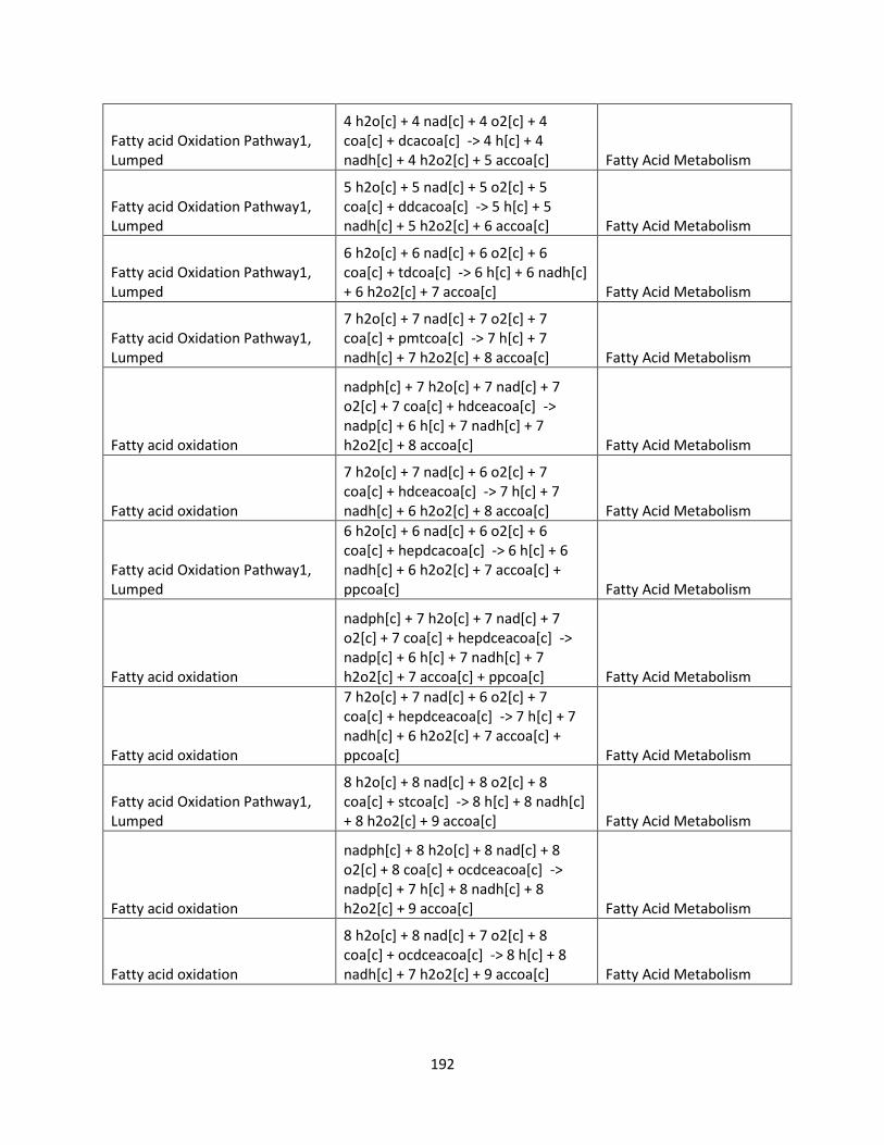
192

Fatty acid Oxidation Pathway1, Lumped

4 h2o[c] + 4 nad[c] + 4 o2[c] + 4 coa[c] + dcacoa[c] -> 4 h[c] + 4 nadh[c] + 4 h2o2[c] + 5 accoa[c] Fatty Acid Metabolism

Fatty acid Oxidation Pathway1, Lumped

5 h2o[c] + 5 nad[c] + 5 o2[c] + 5 coa[c] + ddcacoa[c] -> 5 h[c] + 5 nadh[c] + 5 h2o2[c] + 6 accoa[c] Fatty Acid Metabolism

Fatty acid Oxidation Pathway1, Lumped

6 h2o[c] + 6 nad[c] + 6 o2[c] + 6 coa[c] + tdcoa[c] -> 6 h[c] + 6 nadh[c] + 6 h2o2[c] + 7 accoa[c] Fatty Acid Metabolism

Fatty acid Oxidation Pathway1, Lumped

7 h2o[c] + 7 nad[c] + 7 o2[c] + 7 coa[c] + pmtcoa[c] -> 7 h[c] + 7 nadh[c] + 7 h2o2[c] + 8 accoa[c] Fatty Acid Metabolism

Fatty acid oxidation

nadph[c] + 7 h2o[c] + 7 nad[c] + 7 o2[c] + 7 coa[c] + hdceacoa[c] -> nadp[c] + 6 h[c] + 7 nadh[c] + 7 h2o2[c] + 8 accoa[c] Fatty Acid Metabolism

Fatty acid oxidation

7 h2o[c] + 7 nad[c] + 6 o2[c] + 7 coa[c] + hdceacoa[c] -> 7 h[c] + 7 nadh[c] + 6 h2o2[c] + 8 accoa[c] Fatty Acid Metabolism

Fatty acid Oxidation Pathway1, Lumped

6 h2o[c] + 6 nad[c] + 6 o2[c] + 6 coa[c] + hepdcacoa[c] -> 6 h[c] + 6 nadh[c] + 6 h2o2[c] + 7 accoa[c] + ppcoa[c] Fatty Acid Metabolism

Fatty acid oxidation

nadph[c] + 7 h2o[c] + 7 nad[c] + 7 o2[c] + 7 coa[c] + hepdceacoa[c] -> nadp[c] + 6 h[c] + 7 nadh[c] + 7 h2o2[c] + 7 accoa[c] + ppcoa[c] Fatty Acid Metabolism

Fatty acid oxidation

7 h2o[c] + 7 nad[c] + 6 o2[c] + 7 coa[c] + hepdceacoa[c] -> 7 h[c] + 7 nadh[c] + 6 h2o2[c] + 7 accoa[c] + ppcoa[c] Fatty Acid Metabolism

Fatty acid Oxidation Pathway1, Lumped

8 h2o[c] + 8 nad[c] + 8 o2[c] + 8 coa[c] + stcoa[c] -> 8 h[c] + 8 nadh[c] + 8 h2o2[c] + 9 accoa[c] Fatty Acid Metabolism

Fatty acid oxidation

nadph[c] + 8 h2o[c] + 8 nad[c] + 8 o2[c] + 8 coa[c] + ocdceacoa[c] -> nadp[c] + 7 h[c] + 8 nadh[c] + 8 h2o2[c] + 9 accoa[c] Fatty Acid Metabolism

Fatty acid oxidation

8 h2o[c] + 8 nad[c] + 7 o2[c] + 8 coa[c] + ocdceacoa[c] -> 8 h[c] + 8 nadh[c] + 7 h2o2[c] + 9 accoa[c] Fatty Acid Metabolism

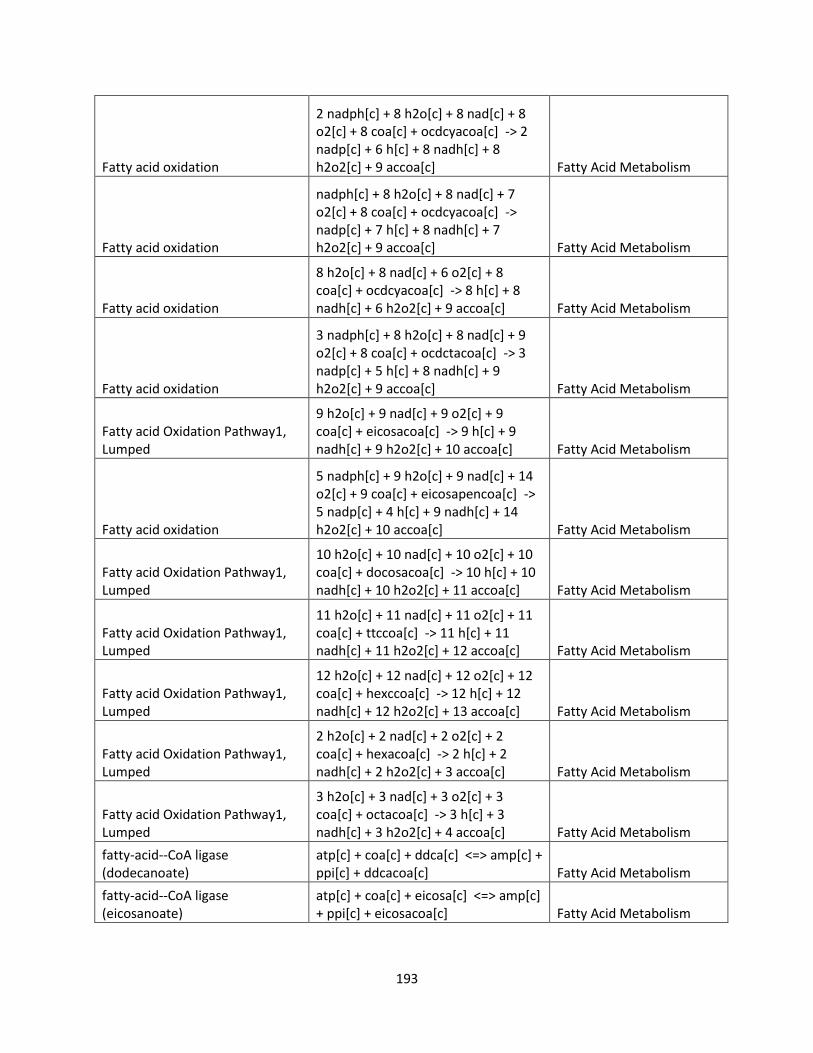
193

Fatty acid oxidation

2 nadph[c] + 8 h2o[c] + 8 nad[c] + 8 o2[c] + 8 coa[c] + ocdcyacoa[c] -> 2 nadp[c] + 6 h[c] + 8 nadh[c] + 8 h2o2[c] + 9 accoa[c] Fatty Acid Metabolism

Fatty acid oxidation

nadph[c] + 8 h2o[c] + 8 nad[c] + 7 o2[c] + 8 coa[c] + ocdcyacoa[c] -> nadp[c] + 7 h[c] + 8 nadh[c] + 7 h2o2[c] + 9 accoa[c] Fatty Acid Metabolism

Fatty acid oxidation

8 h2o[c] + 8 nad[c] + 6 o2[c] + 8 coa[c] + ocdcyacoa[c] -> 8 h[c] + 8 nadh[c] + 6 h2o2[c] + 9 accoa[c] Fatty Acid Metabolism

Fatty acid oxidation

3 nadph[c] + 8 h2o[c] + 8 nad[c] + 9 o2[c] + 8 coa[c] + ocdctacoa[c] -> 3 nadp[c] + 5 h[c] + 8 nadh[c] + 9 h2o2[c] + 9 accoa[c] Fatty Acid Metabolism

Fatty acid Oxidation Pathway1, Lumped

9 h2o[c] + 9 nad[c] + 9 o2[c] + 9 coa[c] + eicosacoa[c] -> 9 h[c] + 9 nadh[c] + 9 h2o2[c] + 10 accoa[c] Fatty Acid Metabolism

Fatty acid oxidation

5 nadph[c] + 9 h2o[c] + 9 nad[c] + 14 o2[c] + 9 coa[c] + eicosapencoa[c] -> 5 nadp[c] + 4 h[c] + 9 nadh[c] + 14 h2o2[c] + 10 accoa[c] Fatty Acid Metabolism

Fatty acid Oxidation Pathway1, Lumped

10 h2o[c] + 10 nad[c] + 10 o2[c] + 10 coa[c] + docosacoa[c] -> 10 h[c] + 10 nadh[c] + 10 h2o2[c] + 11 accoa[c] Fatty Acid Metabolism

Fatty acid Oxidation Pathway1, Lumped

11 h2o[c] + 11 nad[c] + 11 o2[c] + 11 coa[c] + ttccoa[c] -> 11 h[c] + 11 nadh[c] + 11 h2o2[c] + 12 accoa[c] Fatty Acid Metabolism

Fatty acid Oxidation Pathway1, Lumped

12 h2o[c] + 12 nad[c] + 12 o2[c] + 12 coa[c] + hexccoa[c] -> 12 h[c] + 12 nadh[c] + 12 h2o2[c] + 13 accoa[c] Fatty Acid Metabolism

Fatty acid Oxidation Pathway1, Lumped

2 h2o[c] + 2 nad[c] + 2 o2[c] + 2 coa[c] + hexacoa[c] -> 2 h[c] + 2 nadh[c] + 2 h2o2[c] + 3 accoa[c] Fatty Acid Metabolism

Fatty acid Oxidation Pathway1, Lumped

3 h2o[c] + 3 nad[c] + 3 o2[c] + 3 coa[c] + octacoa[c] -> 3 h[c] + 3 nadh[c] + 3 h2o2[c] + 4 accoa[c] Fatty Acid Metabolism

fatty-acid--CoA ligase (dodecanoate)

atp[c] + coa[c] + ddca[c] <=> amp[c] + ppi[c] + ddcacoa[c] Fatty Acid Metabolism

fatty-acid--CoA ligase (eicosanoate)

atp[c] + coa[c] + eicosa[c] <=> amp[c] + ppi[c] + eicosacoa[c] Fatty Acid Metabolism

194

fatty-acid--CoA ligase (docosanoate)

atp[c] + coa[c] + docosa[c] <=> amp[c] + ppi[c] + docosacoa[c] Fatty Acid Metabolism

fatty-acid--CoA ligase (ttc) atp[c] + coa[c] + ttc[c] <=> amp[c] + ppi[c] + ttccoa[c] Fatty Acid Metabolism

fatty-acid--CoA ligase (hexc) atp[c] + coa[c] + hexc[c] <=> amp[c] + ppi[c] + hexccoa[c] Fatty Acid Metabolism

fatty-acid--CoA ligase (octanoate) atp[c] + coa[c] + octa[c] <=> amp[c] + ppi[c] + octacoa[c] Fatty Acid Metabolism

Oleoyl-CoA desaturase (n-C18:1CoA -> n-C18:2CoA)

h[c] + nadph[c] + o2[c] + ocdceacoa[c] -> nadp[c] + 2 h2o[c] + ocdcyacoa[c] Fatty Acid Metabolism

GTP cyclohydrolase I h2o[c] + gtp[c] -> h[c] + for[c] + ahdt[c] Folate Metabolism

5-formethyltetrahydrofolate cyclo-ligase

atp[c] + 5fthf[c] -> adp[c] + pi[c] + methf[c] Folate Metabolism

dihydrofolate reductase (irreversible)

h[c] + nadph[c] + dhf[c] -> nadp[c] + thf[c] Folate Metabolism

4-aminobenzoate synthase 4adcho[c] -> h[c] + pyr[c] + 4abz[c] Folate Metabolism

alkaline phosphatase (Dihydroneopterin)

3 h2o[c] + ahdt[c] -> 2 h[c] + 3 pi[c] + dhnpt[c] Folate Metabolism

Tetrahydrofolate:L-glutamate gamma-ligase (ADP-forming)

atp[c] + glu-L[c] + thf[c] <=> h[c] + adp[c] + pi[c] + thfglu[c] Folate Metabolism

dihydroneopterin aldolase dhnpt[c] -> h[c] + 2ahhmp[c] + gcald[c] Folate Metabolism

dihydropteroate synthase 4abz[c] + 2ahhmp[c] -> h2o[c] + dhpt[c] Folate Metabolism

dihydropteroate synthase 4abz[c] + 2ahhmd[c] -> ppi[c] + dhpt[c] Folate Metabolism

2-amino-4-hydroxy-6-hydroxymethyldihydropteridine diphosphokinase, mitochondrial

atp[c] + 2ahhmp[c] -> h[c] + amp[c] + 2ahhmd[c] Folate Metabolism

5,10-methylenetetrahydrofolate reductase

2 h[c] + nadph[c] + mlthf[c] -> nadp[c] + 5mthf[c] Folate Metabolism

methylenetetrahydrofolate dehydrogenase (NAD)

nad[c] + mlthf[c] -> nadh[c] + methf[c] Folate Metabolism

4-amino-4-deoxychorismate synthase

gln-L[c] + chor[c] -> glu-L[c] + 4adcho[c] Folate Metabolism

formate-tetrahydrofolate ligase, mitochondrial

atp[m] + for[m] + thf[m] -> adp[m] + pi[m] + 10fthf[m] Folate Metabolism

methenyltetrahydrifikate cyclohydrolase, mitochondrial

h2o[m] + methf[m] <=> h[m] + 10fthf[m] Folate Metabolism

195

methylenetetrahydrofolate dehydrogenase (NADP), mitochondrial

nadp[m] + mlthf[m] <=> nadph[m] + methf[m] Folate Metabolism

Methylenetetrahydrofolate dehydrogenase (NADP)

nadp[c] + mlthf[c] <=> nadph[c] + methf[c] Folate Metabolism

tetrahydrofolate aminomethyltransferase, mitochondrial

h2o[m] + methf[m] -> h[m] + 5fthf[m] Folate Metabolism

formate-tetrahydrofolate ligase atp[c] + for[c] + thf[c] -> adp[c] + pi[c] + 10fthf[c] Folate Metabolism

methenyltetrahydrofolate cyclohydrolase h2o[c] + methf[c] <=> h[c] + 10fthf[c] Folate Metabolism

aspartate oxidase fad[m] + asp-L[c] -> fadh2[m] + h[c] + iasp[c] Folate Metabolism

dihydrofolate synthase atp[c] + glu-L[c] + dhpt[c] -> h[c] + adp[c] + pi[c] + dhf[c] Folate Metabolism

5-formethyltetrahydrofolate cyclo-ligase, mitochondrial

atp[m] + 5fthf[m] -> adp[m] + pi[m] + methf[m] Folate Metabolism

L-Fuculose Phosphate Aldolase fuc1p[c] <=> dhap[c] + lald-S[c] Fructose and Mannose Metabolism

hexokinase (D-mannose:ATP) atp[c] + man[c] -> h[c] + adp[c] + man6p[c]

Fructose and mannose metabolism

hexokinase (D-fructose:ATP) atp[c] + fru[c] -> h[c] + adp[c] + f6p[c] Fructose and mannose metabolism

hexokinase (beta D-fructose:ATP) atp[c] + fru[c] -> h[c] + adp[c] + bf6p[c]

Fructose and mannose metabolism

D-sorbitol dehydrogenase (D-fructose producing)

nad[c] + sbt-D[c] -> h[c] + nadh[c] + fru[c]

Fructose and Mannose Metabolism

L-sorbitol dehydrogenase (L-sorbose-producing)

nad[c] + sbt-L[c] -> h[c] + nadh[c] + srb-L[c]

Fructose and Mannose Metabolism

Fructose-2,6-bisphosphatase h2o[c] + bf26p[c] -> pi[c] + bf6p[c] Fructose and mannose metabolism

Fructose-2,6-bisphosphatase 1 h2o[c] + bf26p[c] -> pi[c] + f6p[c] Fructose and mannose metabolism

6-Phosphofructo-2-Kinase atp[c] + bf6p[c] <=> h[c] + adp[c] + bf26p[c]

Fructose and Mannose Metabolism

Mannose-6-phosphate isomerase man6p[c] <=> f6p[c] Fructose and Mannose Metabolism

Mannose-1-phosphate guanylyltransferase

h[c] + gtp[c] + man1p[c] -> ppi[c] + gdpmann[c]

Fructose and Mannose Metabolism

Phosphomannomutase man1p[c] <=> man6p[c] Fructose and Mannose Metabolism

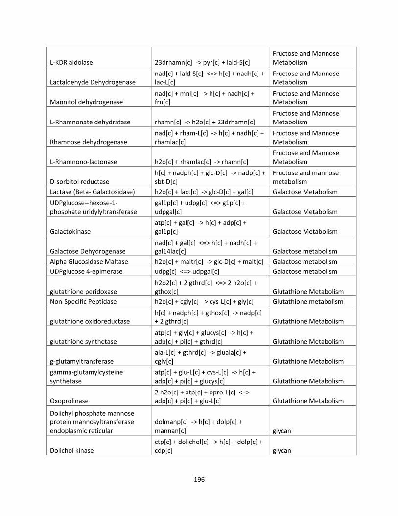
196

L-KDR aldolase 23drhamn[c] -> pyr[c] + lald-S[c] Fructose and Mannose Metabolism

Lactaldehyde Dehydrogenase nad[c] + lald-S[c] <=> h[c] + nadh[c] + lac-L[c]

Fructose and Mannose Metabolism

Mannitol dehydrogenase nad[c] + mnl[c] -> h[c] + nadh[c] + fru[c]

Fructose and Mannose Metabolism

L-Rhamnonate dehydratase rhamn[c] -> h2o[c] + 23drhamn[c] Fructose and Mannose Metabolism

Rhamnose dehydrogenase nad[c] + rham-L[c] -> h[c] + nadh[c] + rhamlac[c]

Fructose and Mannose Metabolism

L-Rhamnono-lactonase h2o[c] + rhamlac[c] -> rhamn[c] Fructose and Mannose Metabolism

D-sorbitol reductase h[c] + nadph[c] + glc-D[c] -> nadp[c] + sbt-D[c]

Fructose and mannose metabolism

Lactase (Beta- Galactosidase) h2o[c] + lact[c] -> glc-D[c] + gal[c] Galactose Metabolism

UDPglucose--hexose-1-phosphate uridylyltransferase

gal1p[c] + udpg[c] <=> g1p[c] + udpgal[c] Galactose Metabolism

Galactokinase atp[c] + gal[c] -> h[c] + adp[c] + gal1p[c] Galactose Metabolism

Galactose Dehydrogenase nad[c] + gal[c] <=> h[c] + nadh[c] + gal14lac[c] Galactose metabolism

Alpha Glucosidase Maltase h2o[c] + maltr[c] -> glc-D[c] + malt[c] Galactose metabolism

UDPglucose 4-epimerase udpg[c] <=> udpgal[c] Galactose metabolism

glutathione peridoxase h2o2[c] + 2 gthrd[c] <=> 2 h2o[c] + gthox[c] Glutathione Metabolism

Non-Specific Peptidase h2o[c] + cgly[c] -> cys-L[c] + gly[c] Glutathione metabolism

glutathione oxidoreductase h[c] + nadph[c] + gthox[c] -> nadp[c] + 2 gthrd[c] Glutathione Metabolism

glutathione synthetase atp[c] + gly[c] + glucys[c] -> h[c] + adp[c] + pi[c] + gthrd[c] Glutathione Metabolism

g-glutamyltransferase ala-L[c] + gthrd[c] -> gluala[c] + cgly[c] Glutathione Metabolism

gamma-glutamylcysteine synthetase

atp[c] + glu-L[c] + cys-L[c] -> h[c] + adp[c] + pi[c] + glucys[c] Glutathione Metabolism

Oxoprolinase 2 h2o[c] + atp[c] + opro-L[c] <=> adp[c] + pi[c] + glu-L[c] Glutathione Metabolism

Dolichyl phosphate mannose protein mannosyltransferase endoplasmic reticular

dolmanp[c] -> h[c] + dolp[c] + mannan[c] glycan

Dolichol kinase ctp[c] + dolichol[c] -> h[c] + dolp[c] + cdp[c] glycan

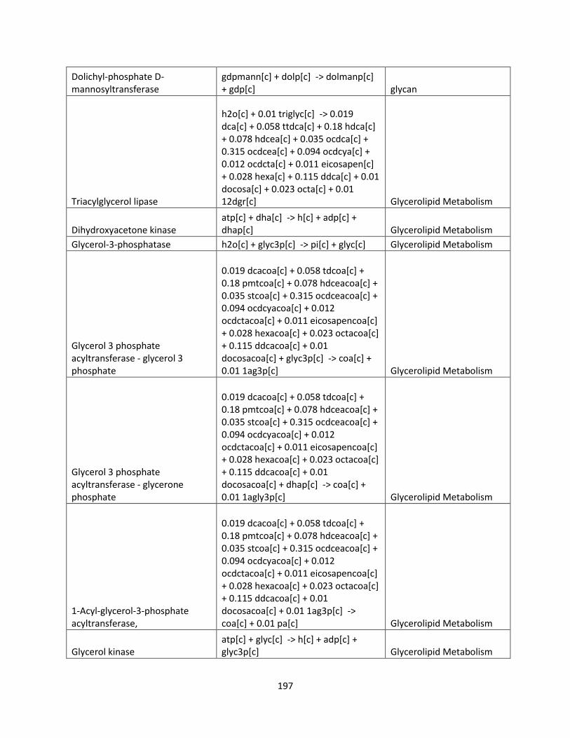
197

Dolichyl-phosphate D-mannosyltransferase

gdpmann[c] + dolp[c] -> dolmanp[c] + gdp[c] glycan

Triacylglycerol lipase

h2o[c] + 0.01 triglyc[c] -> 0.019 dca[c] + 0.058 ttdca[c] + 0.18 hdca[c] + 0.078 hdcea[c] + 0.035 ocdca[c] + 0.315 ocdcea[c] + 0.094 ocdcya[c] + 0.012 ocdcta[c] + 0.011 eicosapen[c] + 0.028 hexa[c] + 0.115 ddca[c] + 0.01 docosa[c] + 0.023 octa[c] + 0.01 12dgr[c] Glycerolipid Metabolism

Dihydroxyacetone kinase atp[c] + dha[c] -> h[c] + adp[c] + dhap[c] Glycerolipid Metabolism

Glycerol-3-phosphatase h2o[c] + glyc3p[c] -> pi[c] + glyc[c] Glycerolipid Metabolism

Glycerol 3 phosphate acyltransferase - glycerol 3 phosphate

0.019 dcacoa[c] + 0.058 tdcoa[c] + 0.18 pmtcoa[c] + 0.078 hdceacoa[c] + 0.035 stcoa[c] + 0.315 ocdceacoa[c] + 0.094 ocdcyacoa[c] + 0.012 ocdctacoa[c] + 0.011 eicosapencoa[c] + 0.028 hexacoa[c] + 0.023 octacoa[c] + 0.115 ddcacoa[c] + 0.01 docosacoa[c] + glyc3p[c] -> coa[c] + 0.01 1ag3p[c] Glycerolipid Metabolism

Glycerol 3 phosphate acyltransferase - glycerone phosphate

0.019 dcacoa[c] + 0.058 tdcoa[c] + 0.18 pmtcoa[c] + 0.078 hdceacoa[c] + 0.035 stcoa[c] + 0.315 ocdceacoa[c] + 0.094 ocdcyacoa[c] + 0.012 ocdctacoa[c] + 0.011 eicosapencoa[c] + 0.028 hexacoa[c] + 0.023 octacoa[c] + 0.115 ddcacoa[c] + 0.01 docosacoa[c] + dhap[c] -> coa[c] + 0.01 1agly3p[c] Glycerolipid Metabolism

1-Acyl-glycerol-3-phosphate acyltransferase,

0.019 dcacoa[c] + 0.058 tdcoa[c] + 0.18 pmtcoa[c] + 0.078 hdceacoa[c] + 0.035 stcoa[c] + 0.315 ocdceacoa[c] + 0.094 ocdcyacoa[c] + 0.012 ocdctacoa[c] + 0.011 eicosapencoa[c] + 0.028 hexacoa[c] + 0.023 octacoa[c] + 0.115 ddcacoa[c] + 0.01 docosacoa[c] + 0.01 1ag3p[c] -> coa[c] + 0.01 pa[c] Glycerolipid Metabolism

Glycerol kinase atp[c] + glyc[c] -> h[c] + adp[c] + glyc3p[c] Glycerolipid Metabolism

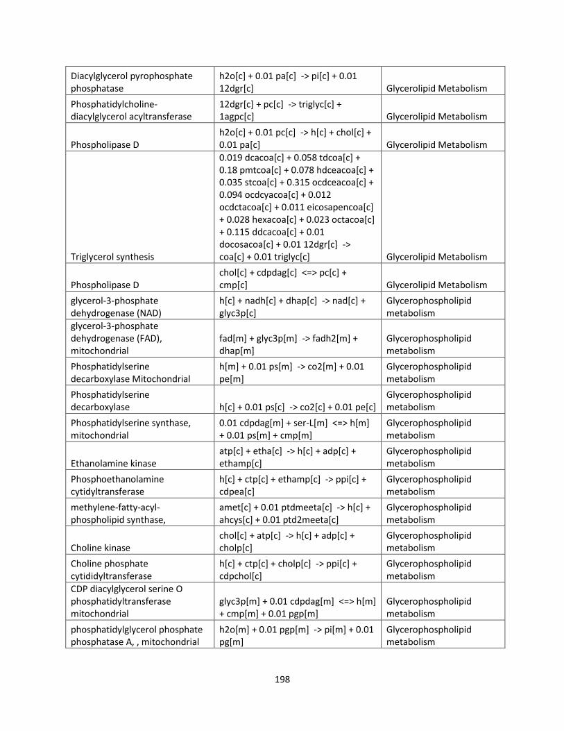
198

Diacylglycerol pyrophosphate phosphatase

h2o[c] + 0.01 pa[c] -> pi[c] + 0.01 12dgr[c] Glycerolipid Metabolism

Phosphatidylcholine-diacylglycerol acyltransferase

12dgr[c] + pc[c] -> triglyc[c] + 1agpc[c] Glycerolipid Metabolism

Phospholipase D h2o[c] + 0.01 pc[c] -> h[c] + chol[c] + 0.01 pa[c] Glycerolipid Metabolism

Triglycerol synthesis

0.019 dcacoa[c] + 0.058 tdcoa[c] + 0.18 pmtcoa[c] + 0.078 hdceacoa[c] + 0.035 stcoa[c] + 0.315 ocdceacoa[c] + 0.094 ocdcyacoa[c] + 0.012 ocdctacoa[c] + 0.011 eicosapencoa[c] + 0.028 hexacoa[c] + 0.023 octacoa[c] + 0.115 ddcacoa[c] + 0.01 docosacoa[c] + 0.01 12dgr[c] -> coa[c] + 0.01 triglyc[c] Glycerolipid Metabolism

Phospholipase D chol[c] + cdpdag[c] <=> pc[c] + cmp[c] Glycerolipid Metabolism

glycerol-3-phosphate dehydrogenase (NAD)

h[c] + nadh[c] + dhap[c] -> nad[c] + glyc3p[c]

Glycerophospholipid metabolism

glycerol-3-phosphate dehydrogenase (FAD), mitochondrial

fad[m] + glyc3p[m] -> fadh2[m] + dhap[m]

Glycerophospholipid metabolism

Phosphatidylserine decarboxylase Mitochondrial

h[m] + 0.01 ps[m] -> co2[m] + 0.01 pe[m]

Glycerophospholipid metabolism

Phosphatidylserine decarboxylase h[c] + 0.01 ps[c] -> co2[c] + 0.01 pe[c]

Glycerophospholipid metabolism

Phosphatidylserine synthase, mitochondrial

0.01 cdpdag[m] + ser-L[m] <=> h[m] + 0.01 ps[m] + cmp[m]

Glycerophospholipid metabolism

Ethanolamine kinase atp[c] + etha[c] -> h[c] + adp[c] + ethamp[c]

Glycerophospholipid metabolism

Phosphoethanolamine cytidyltransferase

h[c] + ctp[c] + ethamp[c] -> ppi[c] + cdpea[c]

Glycerophospholipid metabolism

methylene-fatty-acyl-phospholipid synthase,

amet[c] + 0.01 ptdmeeta[c] -> h[c] + ahcys[c] + 0.01 ptd2meeta[c]

Glycerophospholipid metabolism

Choline kinase chol[c] + atp[c] -> h[c] + adp[c] + cholp[c]

Glycerophospholipid metabolism

Choline phosphate cytididyltransferase

h[c] + ctp[c] + cholp[c] -> ppi[c] + cdpchol[c]

Glycerophospholipid metabolism

CDP diacylglycerol serine O phosphatidyltransferase mitochondrial

glyc3p[m] + 0.01 cdpdag[m] <=> h[m] + cmp[m] + 0.01 pgp[m]

Glycerophospholipid metabolism

phosphatidylglycerol phosphate phosphatase A, , mitochondrial

h2o[m] + 0.01 pgp[m] -> pi[m] + 0.01 pg[m]

Glycerophospholipid metabolism

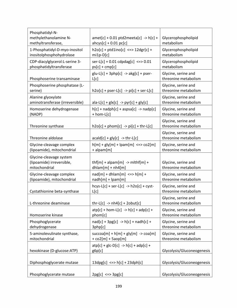
199

Phosphatidyl-N-methylethanolamine N-methyltransferase,

amet[c] + 0.01 ptd2meeta[c] -> h[c] + ahcys[c] + 0.01 pc[c]

Glycerophospholipid metabolism

1-Phosphatidyl-D-myo-inositol inositolphosphohydrolase

h2o[c] + ptd1ino[c] <=> 12dgr[c] + mi1p-D[c]

Glycerophospholipid metabolism

CDP-diacylglycerol:L-serine 3-phosphatidyltransferase

ser-L[c] + 0.01 cdpdag[c] <=> 0.01 ps[c] + cmp[c]

Glycerophospholipid metabolism

Phosphoserine transaminase glu-L[c] + 3php[c] -> akg[c] + pser-L[c]

Glycine, serine and threonine metabolism

Phosphoserine phosphatase (L-serine) h2o[c] + pser-L[c] -> pi[c] + ser-L[c]

Glycine, serine and threonine metabolism

Alanine glyoxylate aminotransferase (irreversible) ala-L[c] + glx[c] -> pyr[c] + gly[c]

Glycine, serine and threonine metabolism

Homoserine dehydrogenase (NADP)

h[c] + nadph[c] + aspsa[c] -> nadp[c] + hom-L[c]

Glycine, serine and threonine metabolism

Threonine synthase h2o[c] + phom[c] -> pi[c] + thr-L[c] Glycine, serine and threonine metabolism

Threonine aldolase acald[c] + gly[c] -> thr-L[c] Glycine, serine and threonine metabolism

Glycine-cleavage complex (lipoamide), mitochondrial

h[m] + gly[m] + lpam[m] <=> co2[m] + alpam[m]

Glycine, serine and threonine metabolism

Glycine-cleavage system (lipoamide) irreversible, mitochondrial

thf[m] + alpam[m] -> mlthf[m] + dhlam[m] + nh4[m]

Glycine, serine and threonine metabolism

Glycine-cleavage complex (lipoamide), mitochondrial

nad[m] + dhlam[m] <=> h[m] + nadh[m] + lpam[m]

Glycine, serine and threonine metabolism

Cystathionine beta-synthase hcys-L[c] + ser-L[c] -> h2o[c] + cyst-L[c]

Glycine, serine and threonine metabolism

L-threonine deaminase thr-L[c] -> nh4[c] + 2obut[c] Glycine, serine and threonine metabolism

Homoserine kinase atp[c] + hom-L[c] -> h[c] + adp[c] + phom[c]

Glycine, serine and threonine metabolism

Phosphoglycerate dehydrogenase

nad[c] + 3pg[c] -> h[c] + nadh[c] + 3php[c]

Glycine, serine and threonine metabolism

5-aminolevulinate synthase, mitochondrial

succoa[m] + h[m] + gly[m] -> coa[m] + co2[m] + 5aop[m]

Glycine, serine and threonine metabolism

hexokinase (D-glucose:ATP) atp[c] + glc-D[c] -> h[c] + adp[c] + g6p[c] Glycolysis/Gluconeogenesis

Diphosphoglycerate mutase 13dpg[c] <=> h[c] + 23dph[c] Glycolysis/Gluconeogenesis

Phosphoglycerate mutase 2pg[c] <=> 3pg[c] Glycolysis/Gluconeogenesis

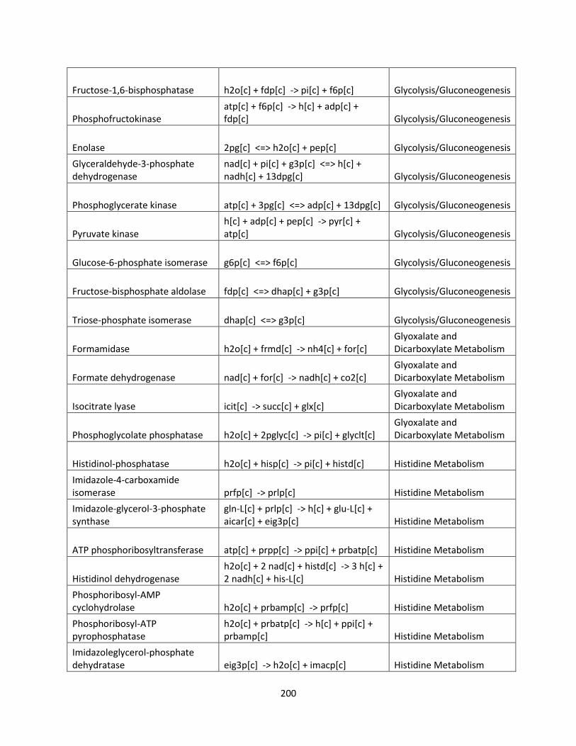
200

Fructose-1,6-bisphosphatase h2o[c] + fdp[c] -> pi[c] + f6p[c] Glycolysis/Gluconeogenesis

Phosphofructokinase atp[c] + f6p[c] -> h[c] + adp[c] + fdp[c] Glycolysis/Gluconeogenesis

Enolase 2pg[c] <=> h2o[c] + pep[c] Glycolysis/Gluconeogenesis

Glyceraldehyde-3-phosphate dehydrogenase

nad[c] + pi[c] + g3p[c] <=> h[c] + nadh[c] + 13dpg[c] Glycolysis/Gluconeogenesis

Phosphoglycerate kinase atp[c] + 3pg[c] <=> adp[c] + 13dpg[c] Glycolysis/Gluconeogenesis

Pyruvate kinase h[c] + adp[c] + pep[c] -> pyr[c] + atp[c] Glycolysis/Gluconeogenesis

Glucose-6-phosphate isomerase g6p[c] <=> f6p[c] Glycolysis/Gluconeogenesis

Fructose-bisphosphate aldolase fdp[c] <=> dhap[c] + g3p[c] Glycolysis/Gluconeogenesis

Triose-phosphate isomerase dhap[c] <=> g3p[c] Glycolysis/Gluconeogenesis

Formamidase h2o[c] + frmd[c] -> nh4[c] + for[c] Glyoxalate and Dicarboxylate Metabolism

Formate dehydrogenase nad[c] + for[c] -> nadh[c] + co2[c] Glyoxalate and Dicarboxylate Metabolism

Isocitrate lyase icit[c] -> succ[c] + glx[c] Glyoxalate and Dicarboxylate Metabolism

Phosphoglycolate phosphatase h2o[c] + 2pglyc[c] -> pi[c] + glyclt[c] Glyoxalate and Dicarboxylate Metabolism

Histidinol-phosphatase h2o[c] + hisp[c] -> pi[c] + histd[c] Histidine Metabolism

Imidazole-4-carboxamide isomerase prfp[c] -> prlp[c] Histidine Metabolism

Imidazole-glycerol-3-phosphate synthase

gln-L[c] + prlp[c] -> h[c] + glu-L[c] + aicar[c] + eig3p[c] Histidine Metabolism

ATP phosphoribosyltransferase atp[c] + prpp[c] -> ppi[c] + prbatp[c] Histidine Metabolism

Histidinol dehydrogenase h2o[c] + 2 nad[c] + histd[c] -> 3 h[c] + 2 nadh[c] + his-L[c] Histidine Metabolism

Phosphoribosyl-AMP cyclohydrolase h2o[c] + prbamp[c] -> prfp[c] Histidine Metabolism

Phosphoribosyl-ATP pyrophosphatase

h2o[c] + prbatp[c] -> h[c] + ppi[c] + prbamp[c] Histidine Metabolism

Imidazoleglycerol-phosphate dehydratase eig3p[c] -> h2o[c] + imacp[c] Histidine Metabolism

201

Histidinol-phosphate transaminase glu-L[c] + imacp[c] -> akg[c] + hisp[c] Histidine metabolism

Phosphatidylinositol synthase 0.01 cdpdag[c] + inost[c] -> h[c] + cmp[c] + 0.01 ptd1ino[c]

Inositol Phosphate Metabolism

Myo-Inositol-1-phosphate synthase g6p[c] -> mi1p-D[c]

Inositol Phosphate Metabolism

1-phosphatidylinositol 3-kinase atp[c] + 0.01 ptd1ino[c] -> h[c] + adp[c] + 0.01 ptd3ino[c]

Inositol Phosphate Metabolism

1-phosphatidylinositol-4,5-bisphosphate phosphodiesterase

h2o[c] + 0.01 ptd145bp[c] -> h[c] + 0.01 12dgr[c] + mi145tp-D[c]

Inositol Phosphate Metabolism

Phosphatidylinositol 4-kinase atp[c] + 0.01 ptd1ino[c] -> h[c] + adp[c] + 0.01 ptd4ino[c]

Inositol Phosphate Metabolism

Inositol-1,4,5-trisphosphate 5-phosphatase

h2o[c] + mi145tp-D[c] -> pi[c] + mi14bp-D[c]

Inositol Phosphate Metabolism

Phosphatidylinositol-3-phosphate 4-kinase

atp[c] + 0.01 ptd3ino[c] -> h[c] + adp[c] + 0.01 ptd134bp[c]

Inositol Phosphate Metabolism

Inositol 2-dehydrogenase nad[c] + inost[c] -> h[c] + nadh[c] + 2ins[c]

Inositol Phosphate Metabolism

Phosphatidylinositol-4-phosphate 5-kinase

atp[c] + 0.01 ptd4ino[c] -> h[c] + adp[c] + 0.01 ptd145bp[c]

Inositol Phosphate Metabolism

Homoisocitrate dehydrogenase, mitochondrial

nad[m] + hicit[m] <=> h[m] + nadh[m] + oxag[m] Lysine Biosynthesis

Dihydrodipicolinate synthase pyr[c] + aspsa[c] -> h[c] + 2 h2o[c] + 23dhdp[c] Lysine Biosynthesis

2-aminoadipate transaminase glu-L[c] + 2oxoadp[c] <=> akg[c] + L2aadp[c] Lysine Biosynthesis

L-aminoadipate-semialdehyde dehydrogenase (NADPH)

h[c] + nadph[c] + atp[c] + L2aadp[c] -> nadp[c] + amp[c] + ppi[c] + L2aadp6sa[c] Lysine Biosynthesis

L-aminoadipate-semialdehyde dehydrogenase (NADH)

h[c] + nadh[c] + atp[c] + L2aadp[c] -> nad[c] + amp[c] + ppi[c] + L2aadp6sa[c] Lysine Biosynthesis

Saccharopine dehydrogenase (NADP, L-glutamate forming)

h[c] + nadph[c] + glu-L[c] + L2aadp6sa[c] <=> nadp[c] + h2o[c] + saccrp-L[c] Lysine Biosynthesis

2-oxoadipate dehydrogenase coa[m] + nad[m] + oxag[m] <=> h[m] + nadh[m] + co2[m] + glucoa[m] Lysine Biosynthesis

Saccharopine dehydrogenase (NAD, L-lysine forming)

h2o[c] + nad[c] + saccrp-L[c] <=> h[c] + nadh[c] + akg[c] + lys-L[c] Lysine Biosynthesis

Homoacontinate hydratase, mitochondrial h2o[m] + b124tc[m] <=> hicit[m] Lysine Biosynthesis

non-enzymatic reaction, mitochondrial

h[m] + oxag[m] <=> co2[m] + 2oxoadp[m] Lysine Biosynthesis

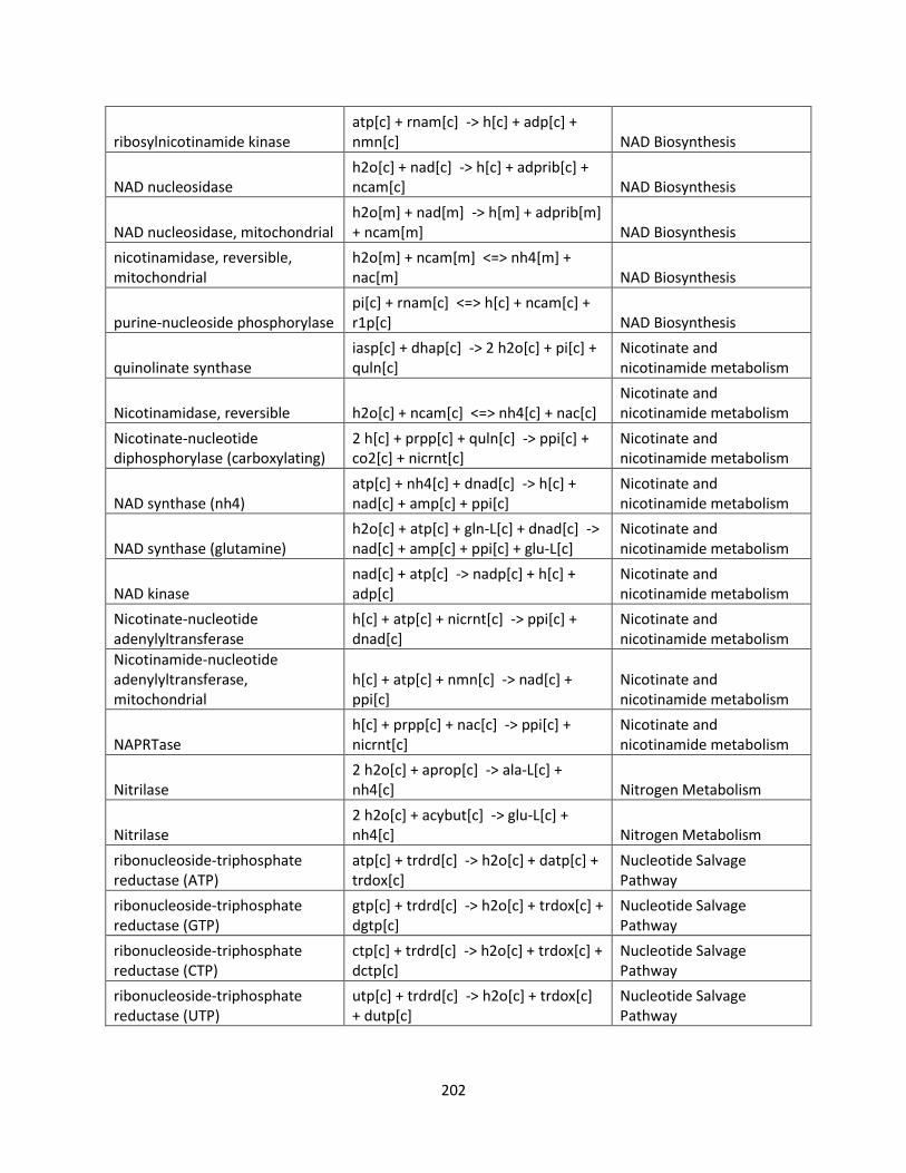
202

ribosylnicotinamide kinase atp[c] + rnam[c] -> h[c] + adp[c] + nmn[c] NAD Biosynthesis

NAD nucleosidase h2o[c] + nad[c] -> h[c] + adprib[c] + ncam[c] NAD Biosynthesis

NAD nucleosidase, mitochondrial h2o[m] + nad[m] -> h[m] + adprib[m] + ncam[m] NAD Biosynthesis

nicotinamidase, reversible, mitochondrial

h2o[m] + ncam[m] <=> nh4[m] + nac[m] NAD Biosynthesis

purine-nucleoside phosphorylase pi[c] + rnam[c] <=> h[c] + ncam[c] + r1p[c] NAD Biosynthesis

quinolinate synthase iasp[c] + dhap[c] -> 2 h2o[c] + pi[c] + quln[c]

Nicotinate and nicotinamide metabolism

Nicotinamidase, reversible h2o[c] + ncam[c] <=> nh4[c] + nac[c] Nicotinate and nicotinamide metabolism

Nicotinate-nucleotide diphosphorylase (carboxylating)

2 h[c] + prpp[c] + quln[c] -> ppi[c] + co2[c] + nicrnt[c]

Nicotinate and nicotinamide metabolism

NAD synthase (nh4) atp[c] + nh4[c] + dnad[c] -> h[c] + nad[c] + amp[c] + ppi[c]

Nicotinate and nicotinamide metabolism

NAD synthase (glutamine) h2o[c] + atp[c] + gln-L[c] + dnad[c] -> nad[c] + amp[c] + ppi[c] + glu-L[c]

Nicotinate and nicotinamide metabolism

NAD kinase nad[c] + atp[c] -> nadp[c] + h[c] + adp[c]

Nicotinate and nicotinamide metabolism

Nicotinate-nucleotide adenylyltransferase

h[c] + atp[c] + nicrnt[c] -> ppi[c] + dnad[c]

Nicotinate and nicotinamide metabolism

Nicotinamide-nucleotide adenylyltransferase, mitochondrial

h[c] + atp[c] + nmn[c] -> nad[c] + ppi[c]

Nicotinate and nicotinamide metabolism

NAPRTase h[c] + prpp[c] + nac[c] -> ppi[c] + nicrnt[c]

Nicotinate and nicotinamide metabolism

Nitrilase 2 h2o[c] + aprop[c] -> ala-L[c] + nh4[c] Nitrogen Metabolism

Nitrilase 2 h2o[c] + acybut[c] -> glu-L[c] + nh4[c] Nitrogen Metabolism

ribonucleoside-triphosphate reductase (ATP)

atp[c] + trdrd[c] -> h2o[c] + datp[c] + trdox[c]

Nucleotide Salvage Pathway

ribonucleoside-triphosphate reductase (GTP)

gtp[c] + trdrd[c] -> h2o[c] + trdox[c] + dgtp[c]

Nucleotide Salvage Pathway

ribonucleoside-triphosphate reductase (CTP)

ctp[c] + trdrd[c] -> h2o[c] + trdox[c] + dctp[c]

Nucleotide Salvage Pathway

ribonucleoside-triphosphate reductase (UTP)

utp[c] + trdrd[c] -> h2o[c] + trdox[c] + dutp[c]

Nucleotide Salvage Pathway

203

Adenine Deaminase h[c] + h2o[c] + ade[c] -> nh4[c] + hxan[c]

Nucleotide Salvage Pathway

Phosphopentomutase 2dr1p[c] <=> 2dr5p[c] Nucleotide Salvage Pathway

CMP nucleosidase h2o[c] + cmp[c] -> csn[c] + r5p[c] Nucleotide Salvage Pathway

Deoxyribose-phosphate aldolase 2dr5p[c] <=> acald[c] + g3p[c] Nucleotide Salvage Pathway

guanosine kinase atp[c] + gsn[c] -> h[c] + adp[c] + gmp[c]

Nucleotide Salvage Pathway

insosine kinase atp[c] + ins[c] -> h[c] + adp[c] + imp[c]

Nucleotide Salvage Pathway

thymidine kinase (ATP:thymidine)

atp[c] + thymd[c] -> h[c] + adp[c] + dtmp[c]

Nucleotide Salvage Pathway

Thymidine phosphorylase pi[c] + thymd[c] <=> 2dr1p[c] + thym[c]

Nucleotide Salvage Pathway

Glycine hydroxymethyltransferase, reversible, mitochondrial

thf[m] + ser-L[m] <=> h2o[m] + mlthf[m] + gly[m] One carbon pool by folate

Glycine hydroxymethyltransferase, reversible

thf[c] + ser-L[c] <=> h2o[c] + gly[c] + mlthf[c] One carbon pool by folate

Adenosinetriphosphatase h2o[c] + atp[c] -> h[c] + adp[c] + pi[c] Oxidative phosphorylation

Succinate Dehydrogenase (Ubiquinone) Mitochondrial

succ[m] + q6[m] <=> fum[m] + q6h2[m] Oxidative Phosphorylation

NADPH dehydrogenase h[c] + nadph[c] + q6[m] -> nadp[c] + q6h2[m] Oxidative Phosphorylation

Ubiquinol-6 cytochrome c reductase

2 h[m] + q6h2[m] + 2 ficytc[m] -> 4 h[c] + q6[m] + 2 focytc[m] Oxidative Phosphorylation

NADPH Quinone reductase h[m] + nadph[m] + q6[m] -> nadp[m] + q6h2[m] Oxidative Phosphorylation

NADH dehydrogenase, with proton transport

5 h[m] + nadh[m] + q6[m] -> 4 h[c] + nad[m] + q6h2[m] Oxidative Phosphorylation

NADPH-ferrihemoprotein reductase

nadph[c] + 2 ficytc[c] -> nadp[c] + h[c] + 2 focytc[c] Oxidative Phosphorylation

Inorganic diphosphatase, mitochondrial h2o[m] + ppi[m] -> 2 pi[m] + h[m] Oxidative Phosphorylation

NADH dehydrogenase, cytoplasmic

h[c] + nadh[c] + q6[m] -> nad[c] + q6h2[m] Oxidative Phosphorylation

Na+/K+-exchanging ATPase h[c] + h2o[c] + atp[c] + k[e] -> adp[c] + pi[c] + h[e] + k[c] Oxidative Phosphorylation

204

Na+/K+-exchanging ATPase h[c] + h2o[c] + atp[c] + Na[e] -> adp[c] + pi[c] + h[e] + Na[c] Oxidative Phosphorylation

Na+/K+-exchanging ATPase h2o[c] + atp[c] + k[e] + Na[c] -> adp[c] + pi[c] + Na[e] + k[c] Oxidative Phosphorylation

Succinate Dehydrogenase (Ubiquinone) Mitochondrial

fadh2[m] + q6[m] -> fad[m] + q6h2[m] Oxidative phosphorylation

NADH dehydrogenase, mitochondrial

h[m] + nadh[m] + q6[m] -> nad[m] + q6h2[m] Oxidative Phosphorylation

Cytochrome c peroxidase, mitochondrial

h2o2[c] + 2 focytc[c] -> 2 h2o[c] + 2 ficytc[c] Oxidative Phosphorylation

Alternative oxidase 0.5 o2[m] + q6h2[m] -> h2o[m] + q6[m] Oxidative Phosphorylation

ATP synthase, mitochondrial adp[m] + pi[m] + 4 h[c] -> atp[m] + h2o[m] + 4 h[m] Oxidative Phosphorylation

cytochrome c oxidase, mitochondrial

8 h[m] + o2[m] + 4 focytc[m] -> 4 h[c] + 2 h2o[m] + 4 ficytc[m] Oxidative Phosphorylation

Inorganic diphosphatase h2o[c] + ppi[c] -> h[c] + 2 pi[c] Oxidative Phosphorylation

ATPase, cytosolic h[c] + h2o[c] + atp[c] -> adp[c] + pi[c] + h[e] Oxidative Phosphorylation

adenylate kinase (Inorganic triphosphate) amp[c] + pppi[c] <=> adp[c] + ppi[c] Oxidative Phosphorylation

Trimetaphosphate hydrolase h2o[c] + tmp[c] <=> h[c] + pppi[c] Oxidative Phosphorylation

GUANPRIBOSYLTRAN-RXN prpp[c] + gua[c] <=> ppi[c] + gmp[c] Oxidative Phosphorylation

purine nucleosidase h2o[c] + gsn[c] <=> rib-D[c] + gua[c] Oxidative Phosphorylation

polyamine oxidase h2o[c] + o2[c] + N1aspmd[c] -> h2o2[c] + aproa[c] + aprut[c]

Pantothenate and CoA Biosynthesis

poylamine oxidase h2o[c] + o2[c] + N1sprm[c] -> h2o2[c] + aproa[c] + N1aspmd[c]

Pantothenate and CoA Biosynthesis

poylamine oxidase h2o[c] + o2[c] + sprm[c] -> h2o2[c] + aproa[c] + spmd[c]

Pantothenate and CoA Biosynthesis

3-methyl-2-oxobutanoate hydroxymethyltransferase

3mob[c] + h2o[c] + mlthf[c] -> thf[c] + 2dhp[c]

Pantotheonate and CoA metabolism

Dephospho-CoA kinase atp[c] + dpcoa[c] -> h[c] + adp[c] + coa[c]

Pantotheonate and CoA metabolism

Pantetheine-phosphate adenylyltransferase

h[c] + atp[c] + pan4p[c] -> ppi[c] + dpcoa[c]

Pantotheonate and CoA metabolism

Phosphopantothenate-cysteine ligase

cys-L[c] + ctp[c] + 4ppan[c] -> h[c] + ppi[c] + cmp[c] + 4ppcys[c]

Pantotheonate and CoA metabolism

2-dehydropantoate 2-reductase, mitochondrial

h[m] + nadph[m] + 2dhp[m] -> nadp[m] + pant-R[m]

Pantotheonate and CoA metabolism

Pantothenate kinase atp[c] + pnto-R[c] -> h[c] + adp[c] + 4ppan[c]

Pantotheonate and CoA metabolism

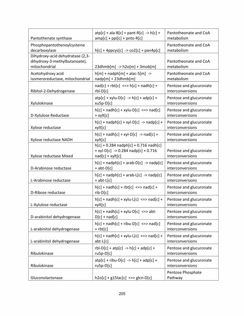
205

Pantothenate synthase atp[c] + ala-B[c] + pant-R[c] -> h[c] + amp[c] + ppi[c] + pnto-R[c]

Pantotheonate and CoA metabolism

Phosphopantothenoylcysteine decarboxylase h[c] + 4ppcys[c] -> co2[c] + pan4p[c]

Pantotheonate and CoA metabolism

Dihydroxy-acid dehydratase (2,3-dihydroxy-3-methylbutanoate), mitochondrial 23dhmb[m] -> h2o[m] + 3mob[m]

Pantotheonate and CoA metabolism

Acetohydroxy acid isomeroreductase, mitochondrial

h[m] + nadph[m] + alac-S[m] -> nadp[m] + 23dhmb[m]

Pantotheonate and CoA metabolism

Ribitol-2-Dehydrogenase nad[c] + rbt[c] <=> h[c] + nadh[c] + rbl-D[c]

Pentose and glucuronate interconversions

Xylulokinase atp[c] + xylu-D[c] -> h[c] + adp[c] + xu5p-D[c]

Pentose and glucuronate interconversions

D-Xylulose Reductase h[c] + nadh[c] + xylu-D[c] <=> nad[c] + xylt[c]

Pentose and glucuronate interconversions

Xylose reductase h[c] + nadph[c] + xyl-D[c] -> nadp[c] + xylt[c]

Pentose and glucuronate interconversions

Xylose reductase NADH h[c] + nadh[c] + xyl-D[c] -> nad[c] + xylt[c]

Pentose and glucuronate interconversions

Xylose reductase Mixed

h[c] + 0.284 nadph[c] + 0.716 nadh[c] + xyl-D[c] -> 0.284 nadp[c] + 0.716 nad[c] + xylt[c]

Pentose and glucuronate interconversions

D-Arabinose reductase h[c] + nadph[c] + arab-D[c] -> nadp[c] + abt-D[c]

Pentose and glucuronate interconversions

L-Arabinose reductase h[c] + nadph[c] + arab-L[c] -> nadp[c] + abt-L[c]

Pentose and glucuronate interconversions

D-Ribose reductase h[c] + nadh[c] + rbt[c] <=> nad[c] + rib-D[c]

Pentose and glucuronate interconversions

L-Xylulose reductase h[c] + nadh[c] + xylu-L[c] <=> nad[c] + xylt[c]

Pentose and glucuronate interconversions

D-arabinitol dehydrogenase h[c] + nadh[c] + xylu-D[c] <=> abt-D[c] + nad[c]

Pentose and glucuronate interconversions

L-arabinitol dehydrogenase h[c] + nadh[c] + ribu-D[c] <=> nad[c] + rbt[c]

Pentose and glucuronate interconversions

L-arabinitol dehydrogenase h[c] + nadh[c] + xylu-L[c] <=> nad[c] + abt-L[c]

Pentose and glucuronate interconversions

Ribulokinase rbl-D[c] + atp[c] -> h[c] + adp[c] + ru5p-D[c]

Pentose and glucuronate interconversions

Ribulokinase atp[c] + ribu-D[c] -> h[c] + adp[c] + ru5p-D[c]

Pentose and glucuronate interconversions

Gluconolactonase h2o[c] + g15lac[c] <=> glcn-D[c] Pentose Phosphate Pathway

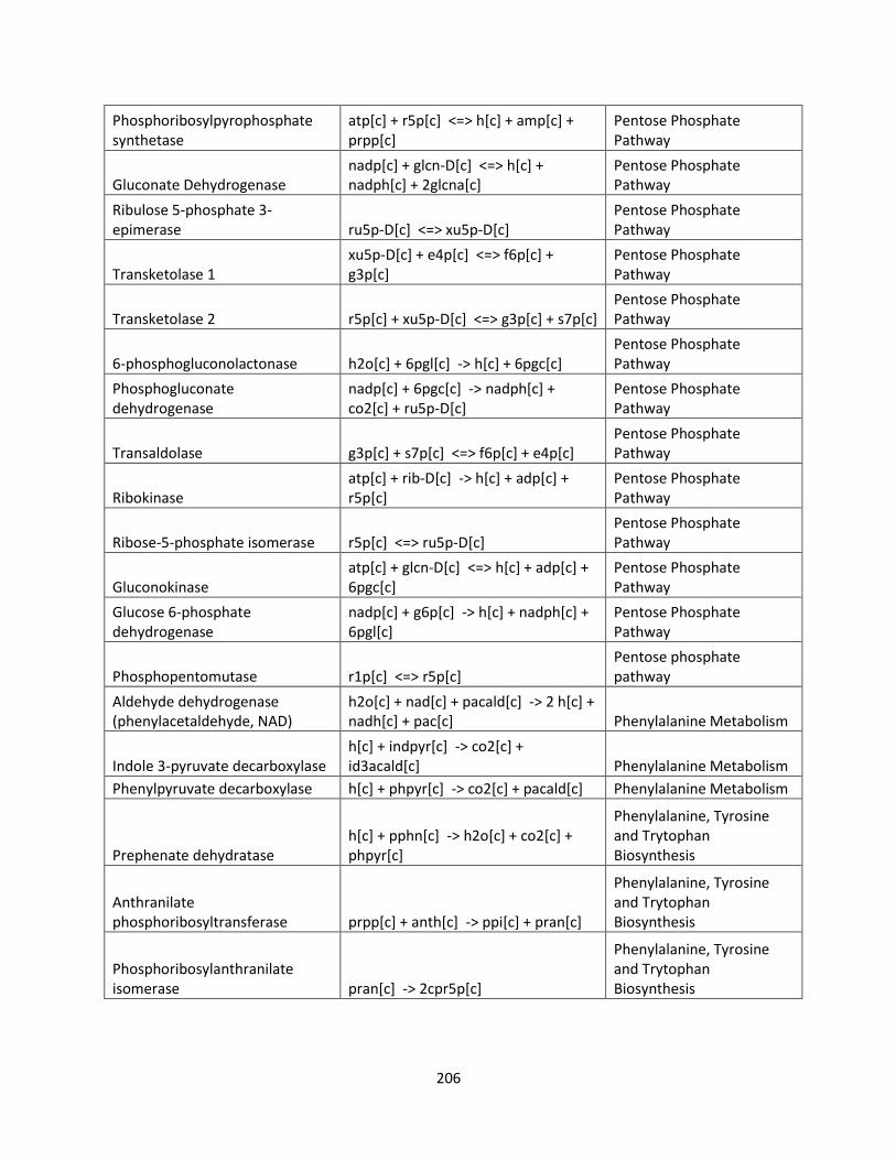
206

Phosphoribosylpyrophosphate synthetase

atp[c] + r5p[c] <=> h[c] + amp[c] + prpp[c]

Pentose Phosphate Pathway

Gluconate Dehydrogenase nadp[c] + glcn-D[c] <=> h[c] + nadph[c] + 2glcna[c]

Pentose Phosphate Pathway

Ribulose 5-phosphate 3-epimerase ru5p-D[c] <=> xu5p-D[c]

Pentose Phosphate Pathway

Transketolase 1 xu5p-D[c] + e4p[c] <=> f6p[c] + g3p[c]

Pentose Phosphate Pathway

Transketolase 2 r5p[c] + xu5p-D[c] <=> g3p[c] + s7p[c] Pentose Phosphate Pathway

6-phosphogluconolactonase h2o[c] + 6pgl[c] -> h[c] + 6pgc[c] Pentose Phosphate Pathway

Phosphogluconate dehydrogenase

nadp[c] + 6pgc[c] -> nadph[c] + co2[c] + ru5p-D[c]

Pentose Phosphate Pathway

Transaldolase g3p[c] + s7p[c] <=> f6p[c] + e4p[c] Pentose Phosphate Pathway

Ribokinase atp[c] + rib-D[c] -> h[c] + adp[c] + r5p[c]

Pentose Phosphate Pathway

Ribose-5-phosphate isomerase r5p[c] <=> ru5p-D[c] Pentose Phosphate Pathway

Gluconokinase atp[c] + glcn-D[c] <=> h[c] + adp[c] + 6pgc[c]

Pentose Phosphate Pathway

Glucose 6-phosphate dehydrogenase

nadp[c] + g6p[c] -> h[c] + nadph[c] + 6pgl[c]

Pentose Phosphate Pathway

Phosphopentomutase r1p[c] <=> r5p[c] Pentose phosphate pathway

Aldehyde dehydrogenase (phenylacetaldehyde, NAD)

h2o[c] + nad[c] + pacald[c] -> 2 h[c] + nadh[c] + pac[c] Phenylalanine Metabolism

Indole 3-pyruvate decarboxylase h[c] + indpyr[c] -> co2[c] + id3acald[c] Phenylalanine Metabolism

Phenylpyruvate decarboxylase h[c] + phpyr[c] -> co2[c] + pacald[c] Phenylalanine Metabolism

Prephenate dehydratase h[c] + pphn[c] -> h2o[c] + co2[c] + phpyr[c]

Phenylalanine, Tyrosine and Trytophan Biosynthesis

Anthranilate phosphoribosyltransferase prpp[c] + anth[c] -> ppi[c] + pran[c]

Phenylalanine, Tyrosine and Trytophan Biosynthesis

Phosphoribosylanthranilate isomerase pran[c] -> 2cpr5p[c]

Phenylalanine, Tyrosine and Trytophan Biosynthesis

207

Tyrosine transaminase, mitochondrial

akg[m] + tyr-L[m] <=> glu-L[m] + 34hpp[m]

Phenylalanine, Tyrosine and Trytophan Biosynthesis

Prephenate dehydrogenase (NADP)

nadp[c] + pphn[c] -> nadph[c] + co2[c] + 34hpp[c]

Phenylalanine, Tyrosine and Trytophan Biosynthesis

3-dehydroquinate dehydratase 3dhq[c] -> h2o[c] + 3dhsk[c]

Phenylalanine, Tyrosine and Trytophan Biosynthesis

Tyrosine transaminase akg[c] + tyr-L[c] <=> glu-L[c] + 34hpp[c]

Phenylalanine, Tyrosine and Trytophan Biosynthesis

Phenylalanine transaminase akg[c] + phe-L[c] <=> glu-L[c] + phpyr[c]

Phenylalanine, Tyrosine and Trytophan Biosynthesis

tryptophan transaminase akg[c] + trp-L[c] <=> glu-L[c] + indpyr[c]

Phenylalanine, Tyrosine and Trytophan Biosynthesis

Tyrosine transaminase glu-L[c] + 34hpp[c] -> akg[c] + tyr-L[c]

Phenylalanine, Tyrosine and Trytophan Biosynthesis

Tryptophan synthase (indoleglycerol phosphate)

ser-L[c] + 3ig3p[c] -> h2o[c] + g3p[c] + trp-L[c]

Phenylalanine, Tyrosine and Trytophan Biosynthesis

Chorismate mutase chor[c] -> pphn[c]

Phenylalanine, Tyrosine and Trytophan Biosynthesis

Anthranilate synthase gln-L[c] + chor[c] -> h[c] + pyr[c] + glu-L[c] + anth[c]

Phenylalanine, Tyrosine and Trytophan Biosynthesis

3-deoxy-D-arabino-heptulosonate 7-phosphate synthetase

h2o[c] + pep[c] + e4p[c] -> pi[c] + 2dda7p[c]

Phenylalanine, Tyrosine and Trytophan Biosynthesis

3-dehydroquinate synthase 2dda7p[c] -> pi[c] + 3dhq[c]

Phenylalanine, Tyrosine and Trytophan Biosynthesis

3-phosphoshikimate 1-carboxyvinyltransferase pep[c] + skm5p[c] -> pi[c] + 3psme[c]

Phenylalanine, Tyrosine and Trytophan Biosynthesis

shikimate dehydrogenase h[c] + nadph[c] + 3dhsk[c] -> nadp[c] + skm[c]

Phenylalanine, Tyrosine and Trytophan Biosynthesis

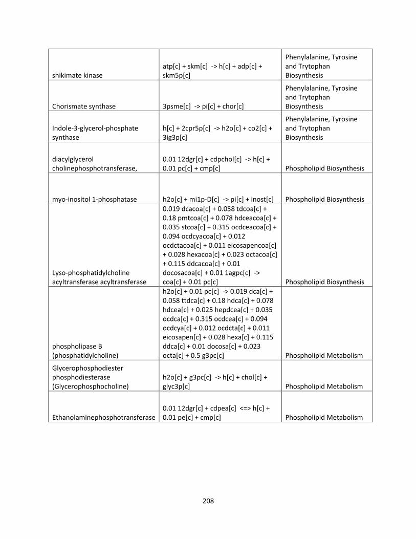
208

shikimate kinase atp[c] + skm[c] -> h[c] + adp[c] + skm5p[c]

Phenylalanine, Tyrosine and Trytophan Biosynthesis

Chorismate synthase 3psme[c] -> pi[c] + chor[c]

Phenylalanine, Tyrosine and Trytophan Biosynthesis

Indole-3-glycerol-phosphate synthase

h[c] + 2cpr5p[c] -> h2o[c] + co2[c] + 3ig3p[c]

Phenylalanine, Tyrosine and Trytophan Biosynthesis

diacylglycerol cholinephosphotransferase,

0.01 12dgr[c] + cdpchol[c] -> h[c] + 0.01 pc[c] + cmp[c] Phospholipid Biosynthesis

myo-inositol 1-phosphatase h2o[c] + mi1p-D[c] -> pi[c] + inost[c] Phospholipid Biosynthesis

Lyso-phosphatidylcholine acyltransferase acyltransferase

0.019 dcacoa[c] + 0.058 tdcoa[c] + 0.18 pmtcoa[c] + 0.078 hdceacoa[c] + 0.035 stcoa[c] + 0.315 ocdceacoa[c] + 0.094 ocdcyacoa[c] + 0.012 ocdctacoa[c] + 0.011 eicosapencoa[c] + 0.028 hexacoa[c] + 0.023 octacoa[c] + 0.115 ddcacoa[c] + 0.01 docosacoa[c] + 0.01 1agpc[c] -> coa[c] + 0.01 pc[c] Phospholipid Biosynthesis

phospholipase B (phosphatidylcholine)

h2o[c] + 0.01 pc[c] -> 0.019 dca[c] + 0.058 ttdca[c] + 0.18 hdca[c] + 0.078 hdcea[c] + 0.025 hepdcea[c] + 0.035 ocdca[c] + 0.315 ocdcea[c] + 0.094 ocdcya[c] + 0.012 ocdcta[c] + 0.011 eicosapen[c] + 0.028 hexa[c] + 0.115 ddca[c] + 0.01 docosa[c] + 0.023 octa[c] + 0.5 g3pc[c] Phospholipid Metabolism

Glycerophosphodiester phosphodiesterase (Glycerophosphocholine)

h2o[c] + g3pc[c] -> h[c] + chol[c] + glyc3p[c] Phospholipid Metabolism

Ethanolaminephosphotransferase 0.01 12dgr[c] + cdpea[c] <=> h[c] + 0.01 pe[c] + cmp[c] Phospholipid Metabolism

209

phospholipase B (phosphatidylinositol)

h2o[e] + 0.005 ptd1ino[e] -> 0.019 dca[e] + 0.115 ddca[e] + 0.01 docosa[e] + 0.011 eicosapen[e] + 0.5 g3pi[e] + 0.18 hdca[e] + 0.078 hdcea[e] + 0.025 hepdcea[e] + 0.028 hexa[e] + 0.035 ocdca[e] + 0.315 ocdcea[e] + 0.012 ocdcta[e] + 0.094 ocdcya[e] + 0.058 ttdca[e] + 0.023 octa[e]

Phospholipid Metabolism

phospholipase B (phosphatidylcholine)

h2o[e] + 0.005 pc[e] -> 0.019 dca[e] + 0.115 ddca[e] + 0.01 docosa[e] + 0.011 eicosapen[e] + 0.5 g3pc[e] + 0.18 hdca[e] + 0.078 hdcea[e] + 0.025 hepdcea[e] + 0.028 hexa[e] + 0.035 ocdca[e] + 0.315 ocdcea[e] + 0.012 ocdcta[e] + 0.094 ocdcya[e] + 0.058 ttdca[e] + 0.023 octa[e]

Phospholipid Metabolism

Cardiolipin synthase, mitochondrial

0.01 cdpdag[m] + 0.01 pg[m] -> h[m] + cmp[m] + 0.01 clpn[m]

Phospholipid Metabolism

Phosphatidylethanolamine N methyltransferase

amet[c] + 0.01 pe[c] -> h[c] + ahcys[c] + 0.01 ptdmeeta[c]

Phospholipid Metabolism

CDP Diacylglycerol synthetase h[c] + ctp[c] + 0.01 pa[c] <=> ppi[c] + 0.01 cdpdag[c]

Phospholipid Metabolism

CDP Diacylglycerol synthetase, Mitochondrial

h[m] + ctp[m] + 0.01 pa[m] <=> 0.01 cdpdag[m] + ppi[m]

Phospholipid Metabolism

uroporphyrinogen methyltransferase 2 amet[c] + uppg3[c] -> h[c] + 2 ahcys[c] + dscl[c]

Porphyrin and chlorophyll metabolism

Ferrochelatase, mitochondrial fe2[m] + ppp9[m] -> 2 h[m] + pheme[m]

Porphyrin and chlorophyll metabolism

uroporphyrinogen decarboxylase (uroporphyrinogen III)

4 h[c] + uppg3[c] -> 4 co2[c] + cpppg3[c]

Porphyrin and chlorophyll metabolism

hydroxymethylbilane synthase h2o[c] + 4 ppbng[c] -> 4 nh4[c] + hmbil[c]

Porphyrin and chlorophyll metabolism

Heme O synthase, mitochondrial h2o[m] + pheme[m] + frdp[m] -> ppi[m] + hemeO[m]

Porphyrin and chlorophyll metabolism

porphobilinogen synthase 2 5aop[c] -> h[c] + 2 h2o[c] + ppbng[c]

Porphyrin and chlorophyll metabolism

protoporphyrinogen oxidase, mitochondrial 3 o2[m] + 2 pppg9[m] -> 6 h2o[m] + 2 ppp9[m]

Porphyrin and chlorophyll metabolism

210

uroporphyrinogen-III synthase hmbil[c] -> h2o[c] + uppg3[c] Porphyrin and chlorophyll metabolism

sirohydrochlorin dehydrogenase nadp[c] + dscl[c] -> h[c] + nadph[c] + scl[c]

Porphyrin and chlorophyll metabolism

sirohydrochlorin ferrochetalase scl[c] + fe2[c] -> 3 h[c] + sheme[c]

Porphyrin and chlorophyll metabolism

coproporphyrinogen oxidase (O2 required) 2 h[c] + o2[c] + cpppg3[c] -> 2 h2o[c] + 2 co2[c] + pppg9[c]

Porphyrin and chlorophyll metabolism

Heme O monooxygenase, mitochondrial

nadh[m] + o2[m] + hemeO[m] -> h2o[m] + nad[m] + hemeA[m]

Porphyrin and chlorophyll metabolism

2-methylcitrate synthase oaa[m] + h2o[m] + ppcoa[m] -> coa[m] + 2mcit[m] + h[m]

Propanoate metabolism

3-Hydroxypropionyl-CoA hydro-lyase h2o[c] + ppcoa[c] <=> hppcoa[c]

Propanoate Metabolism

Acyl-CoA Dehydrogenase ppcoa[c] + fad[c] <=> fadh2[c] + ppecoa[c]

Propanoate Metabolism

Beta-alanine:2-oxoglutarate aminotransferase

akg[c] + ala-B[c] <=> glu-L[c] + msa[c]

Propanoate Metabolism

Methylmalonate-semialdehyde dehydrogenase, Mitochondrial

coa[m] + nad[m] + 2mop[m] -> nadh[m] + co2[m] + ppcoa[m]

Propanoate Metabolism

Adenine phosphoribosyltransferase prpp[c] + ade[c] -> amp[c] + ppi[c] Purine Metabolism

Ribonucleoside-diphosphate reductase (ADP)

adp[c] + trdrd[c] -> h2o[c] + trdox[c] + dadp[c] Purine Metabolism

Ribonucleoside-diphosphate reductase (GDP)

gdp[c] + trdrd[c] -> h2o[c] + trdox[c] + dgdp[c] Purine Metabolism

5'-nucleotidase (XMP) h2o[c] + xmp[c] -> pi[c] + xtsn[c] Purine Metabolism

5'-nucleotidase (UMP) h2o[c] + ump[c] -> pi[c] + uri[c] Purine Metabolism

5'-nucleotidase (dCMP) h2o[c] + dcmp[c] -> pi[c] + dcyt[c] Purine Metabolism

5'-nucleotidase (dTMP) h2o[c] + dtmp[c] -> pi[c] + thymd[c] Purine Metabolism

5'-nucleotidase (dAMP) h2o[c] + damp[c] -> pi[c] + dad-2[c] Purine Metabolism

5'-nucleotidase (AMP) h2o[c] + amp[c] -> pi[c] + adn[c] Purine Metabolism

5'-nucleotidase (dGMP) h2o[c] + dgmp[c] -> pi[c] + dgsn[c] Purine Metabolism

211

5'-nucleotidase (GMP) h2o[c] + gmp[c] -> pi[c] + gsn[c] Purine Metabolism

Phosphoribosylglycinamide formyltransferase

10fthf[c] + gar[c] -> h[c] + thf[c] + fgam[c] Purine Metabolism

Allantoinase h2o[c] + alltn[c] -> alltt[c] Purine Metabolism

Guanine deaminase h[c] + h2o[c] + gua[c] -> nh4[c] + xan[c] Purine Metabolism

Uricase 2 h2o[c] + o2[c] + urate[c] -> co2[c] + h2o2[c] + alltn[c] Purine Metabolism

Adenosine monophosphate deaminase h[c] + h2o[c] + amp[c] -> nh4[c] + imp[c] Purine Metabolism

Bis(5'-adenosyl)-tetraphosphatase h2o[c] + ap4a[c] -> atp[c] + amp[c] Purine Metabolism

Bis(5'-Guanosyl)-tetraphosphatase h2o[c] + gp4g[c] -> gtp[c] + gmp[c] Purine Metabolism

Bis(5'-Uridyl)-tetraphosphatase h2o[c] + up4u[c] -> utp[c] + ump[c] Purine Metabolism

Bis(5'-Xanthosyl)-tetraphosphatase h2o[c] + xp4x[c] -> xmp[c] + xtp[c] Purine Metabolism

Ureidoglycolate hydrolase h2o[c] + urdglyc[c] -> co2[c] + 2 nh4[c] + glx[c] Purine Metabolism

ATP adenylyltransferase h[c] + adp[c] + gtp[c] -> pi[c] + ap4g[c] Purine Metabolism

ATP adenylyltransferase h[c] + gtp[c] + gdp[c] -> pi[c] + gp4g[c] Purine Metabolism

Phosphoribosyl aminoimidazole succinocarboxamide synthase

atp[c] + asp-L[c] + 5aizc[c] <=> h[c] + adp[c] + pi[c] + 25aics[c] Purine Metabolism

Allantoate aminohydrolase h2o[c] + alltt[c] <=> urea[c] + urdglyc[c] Purine Metabolism

Adenosine kinase atp[c] + adn[c] -> h[c] + adp[c] + amp[c] Purine Metabolism

Adenosine deaminase h[c] + h2o[c] + adn[c] -> nh4[c] + ins[c] Purine Metabolism

Ap4A hydrolase h2o[c] + ap4a[c] -> 2 h[c] + 2 adp[c] Purine Metabolism

adenylate kinase, mitochondrial atp[m] + amp[m] <=> 2 adp[m] Purine Metabolism

adenylate kinase atp[c] + amp[c] <=> 2 adp[c] Purine Metabolism

IMP dehydrogenase h2o[c] + nad[c] + imp[c] -> h[c] + nadh[c] + xmp[c] Purine Metabolism

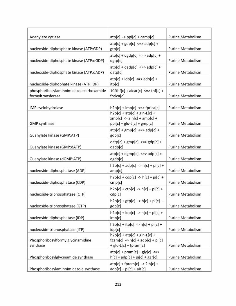
212

Adenylate cyclase atp[c] -> ppi[c] + camp[c] Purine Metabolism

nucleoside-diphosphate kinase (ATP:GDP) atp[c] + gdp[c] <=> adp[c] + gtp[c] Purine Metabolism

nucleoside-diphosphate kinase (ATP:dGDP) atp[c] + dgdp[c] <=> adp[c] + dgtp[c] Purine Metabolism

nucleoside-diphosphate kinase (ATP:dADP) atp[c] + dadp[c] <=> adp[c] + datp[c] Purine Metabolism

nucleoside-diphophate kinase (ATP:IDP) atp[c] + idp[c] <=> adp[c] + itp[c] Purine Metabolism

phosphoribosylaminoimidazolecarboxamide formyltransferase

10fthf[c] + aicar[c] <=> thf[c] + fprica[c] Purine Metabolism

IMP cyclohydrolase h2o[c] + imp[c] <=> fprica[c] Purine Metabolism

GMP synthase

h2o[c] + atp[c] + gln-L[c] + xmp[c] -> 2 h[c] + amp[c] + ppi[c] + glu-L[c] + gmp[c] Purine Metabolism

Guanylate kinase (GMP:ATP) atp[c] + gmp[c] <=> adp[c] + gdp[c] Purine Metabolism

Guanylate kinase (GMP:dATP) datp[c] + gmp[c] <=> gdp[c] + dadp[c] Purine Metabolism

Guanylate kinase (dGMP:ATP) atp[c] + dgmp[c] <=> adp[c] + dgdp[c] Purine Metabolism

nucleoside-diphosphatase (ADP) h2o[c] + adp[c] -> h[c] + pi[c] + amp[c] Purine Metabolism

nucleoside-diphosphatase (CDP) h2o[c] + cdp[c] -> h[c] + pi[c] + cmp[c] Purine Metabolism

nucleoside-triphosphatase (CTP) h2o[c] + ctp[c] -> h[c] + pi[c] + cdp[c] Purine Metabolism

nucleoside-triphosphatase (GTP) h2o[c] + gtp[c] -> h[c] + pi[c] + gdp[c] Purine Metabolism

nucleoside-diphosphatase (IDP) h2o[c] + idp[c] -> h[c] + pi[c] + imp[c] Purine Metabolism

nucleoside-triphosphatase (ITP) h2o[c] + itp[c] -> h[c] + pi[c] + idp[c] Purine Metabolism

Phosphoribosylformylglycinamidine synthase

h2o[c] + atp[c] + gln-L[c] + fgam[c] -> h[c] + adp[c] + pi[c] + glu-L[c] + fpram[c] Purine Metabolism

Phosphoribosylglycinamide synthase atp[c] + pram[c] + gly[c] <=> h[c] + adp[c] + pi[c] + gar[c] Purine Metabolism

Phosphoribosylaminoimidazole synthase atp[c] + fpram[c] -> 2 h[c] + adp[c] + pi[c] + air[c] Purine Metabolism

213

3',5'-cyclic-nucleotide phosphodiesterase h2o[c] + camp[c] -> h[c] + amp[c] Purine Metabolism

Phosphoribosylaminoimidazole carboxylase co2[c] + air[c] <=> h[c] + 5aizc[c] Purine Metabolism

nucleoside-diphosphatase (GDP) h2o[c] + gdp[c] -> h[c] + pi[c] + gmp[c] Purine Metabolism

nucleoside-diphosphatase (UDP) h2o[c] + udp[c] -> h[c] + pi[c] + ump[c] Purine Metabolism

Pyruvate kinase GDP h[c] + gdp[c] + pep[c] -> pyr[c] + gtp[c] Purine Metabolism

Adenylsuccinate lyase dcamp[c] <=> fum[c] + amp[c] Purine Metabolism

Adenylosuccinate lyase 25aics[c] <=> fum[c] + aicar[c] Purine Metabolism

Adenylosuccinate synthase asp-L[c] + gtp[c] + imp[c] -> 2 h[c] + pi[c] + gdp[c] + dcamp[c] Purine Metabolism

deoxyuridine kinase (ATP:Deoxyuridine)

atp[c] + duri[c] -> h[c] + adp[c] + dump[c] Purine Metabolism

purine nucleoside phosphorylase Xanthosine pi[c] + xtsn[c] <=> r1p[c] + xan[c] Purine Metabolism

xanthine dehydrogenase h2o[c] + nad[c] + hxan[c] -> h[c] + nadh[c] + xan[c] Purine Metabolism

xanthine dehydrogenase h2o[c] + nad[c] + xan[c] -> h[c] + nadh[c] + urate[c] Purine Metabolism

Adenylyl-sulfate kinase atp[c] + aps[c] -> h[c] + paps[c] + adp[c] Purine Metabolism

Deoxyadenosine deaminase h[c] + h2o[c] + dad-2[c] -> nh4[c] + din[c] Purine Metabolism

deoxyadenylate kinase atp[c] + damp[c] <=> adp[c] + dadp[c] Purine Metabolism

purine nucleoside phosphorylase Adenosine pi[c] + adn[c] <=> ade[c] + r1p[c] Purine Metabolism

purine-nucleoside phosphorylase (Deoxyadenosine) pi[c] + dad-2[c] <=> ade[c] + 2dr1p[c] Purine Metabolism

purine nucleoside phosphorylase Guanosine pi[c] + gsn[c] <=> r1p[c] + gua[c] Purine Metabolism

purine-nucleoside phosphorylase (Deoxyguanosine) pi[c] + dgsn[c] <=> 2dr1p[c] + gua[c] Purine Metabolism

purine nucleoside phosphorylase Inosine pi[c] + ins[c] <=> r1p[c] + hxan[c] Purine Metabolism

purine-nucleoside phosphorylase (Deoxyinosine) pi[c] + din[c] <=> hxan[c] + 2dr1p[c] Purine Metabolism

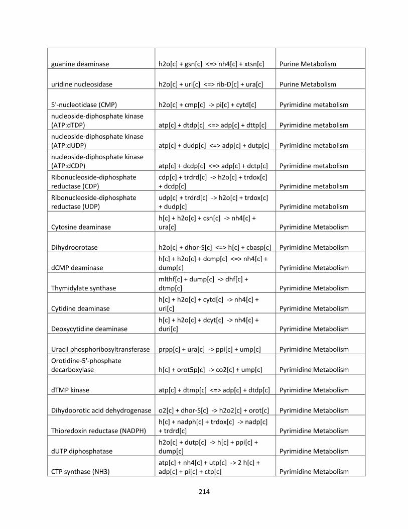
214

guanine deaminase h2o[c] + gsn[c] <=> nh4[c] + xtsn[c] Purine Metabolism

uridine nucleosidase h2o[c] + uri[c] <=> rib-D[c] + ura[c] Purine Metabolism

5'-nucleotidase (CMP) h2o[c] + cmp[c] -> pi[c] + cytd[c] Pyrimidine metabolism

nucleoside-diphosphate kinase (ATP:dTDP) atp[c] + dtdp[c] <=> adp[c] + dttp[c] Pyrimidine metabolism

nucleoside-diphosphate kinase (ATP:dUDP) atp[c] + dudp[c] <=> adp[c] + dutp[c] Pyrimidine metabolism

nucleoside-diphosphate kinase (ATP:dCDP) atp[c] + dcdp[c] <=> adp[c] + dctp[c] Pyrimidine metabolism

Ribonucleoside-diphosphate reductase (CDP)

cdp[c] + trdrd[c] -> h2o[c] + trdox[c] + dcdp[c] Pyrimidine metabolism

Ribonucleoside-diphosphate reductase (UDP)

udp[c] + trdrd[c] -> h2o[c] + trdox[c] + dudp[c] Pyrimidine metabolism

Cytosine deaminase h[c] + h2o[c] + csn[c] -> nh4[c] + ura[c] Pyrimidine Metabolism

Dihydroorotase h2o[c] + dhor-S[c] <=> h[c] + cbasp[c] Pyrimidine Metabolism

dCMP deaminase h[c] + h2o[c] + dcmp[c] <=> nh4[c] + dump[c] Pyrimidine Metabolism

Thymidylate synthase mlthf[c] + dump[c] -> dhf[c] + dtmp[c] Pyrimidine Metabolism

Cytidine deaminase h[c] + h2o[c] + cytd[c] -> nh4[c] + uri[c] Pyrimidine Metabolism

Deoxycytidine deaminase h[c] + h2o[c] + dcyt[c] -> nh4[c] + duri[c] Pyrimidine Metabolism

Uracil phosphoribosyltransferase prpp[c] + ura[c] -> ppi[c] + ump[c] Pyrimidine Metabolism

Orotidine-5'-phosphate decarboxylase h[c] + orot5p[c] -> co2[c] + ump[c] Pyrimidine Metabolism

dTMP kinase atp[c] + dtmp[c] <=> adp[c] + dtdp[c] Pyrimidine Metabolism

Dihydoorotic acid dehydrogenase o2[c] + dhor-S[c] -> h2o2[c] + orot[c] Pyrimidine Metabolism

Thioredoxin reductase (NADPH) h[c] + nadph[c] + trdox[c] -> nadp[c] + trdrd[c] Pyrimidine Metabolism

dUTP diphosphatase h2o[c] + dutp[c] -> h[c] + ppi[c] + dump[c] Pyrimidine Metabolism

CTP synthase (NH3) atp[c] + nh4[c] + utp[c] -> 2 h[c] + adp[c] + pi[c] + ctp[c] Pyrimidine Metabolism

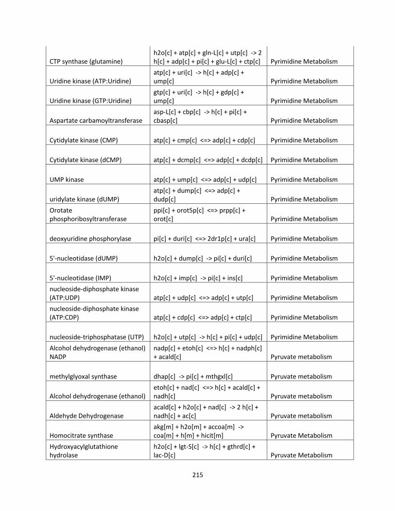
215

CTP synthase (glutamine) h2o[c] + atp[c] + gln-L[c] + utp[c] -> 2 h[c] + adp[c] + pi[c] + glu-L[c] + ctp[c] Pyrimidine Metabolism

Uridine kinase (ATP:Uridine) atp[c] + uri[c] -> h[c] + adp[c] + ump[c] Pyrimidine Metabolism

Uridine kinase (GTP:Uridine) gtp[c] + uri[c] -> h[c] + gdp[c] + ump[c] Pyrimidine Metabolism

Aspartate carbamoyltransferase asp-L[c] + cbp[c] -> h[c] + pi[c] + cbasp[c] Pyrimidine Metabolism

Cytidylate kinase (CMP) atp[c] + cmp[c] <=> adp[c] + cdp[c] Pyrimidine Metabolism

Cytidylate kinase (dCMP) atp[c] + dcmp[c] <=> adp[c] + dcdp[c] Pyrimidine Metabolism

UMP kinase atp[c] + ump[c] <=> adp[c] + udp[c] Pyrimidine Metabolism

uridylate kinase (dUMP) atp[c] + dump[c] <=> adp[c] + dudp[c] Pyrimidine Metabolism

Orotate phosphoribosyltransferase

ppi[c] + orot5p[c] <=> prpp[c] + orot[c] Pyrimidine Metabolism

deoxyuridine phosphorylase pi[c] + duri[c] <=> 2dr1p[c] + ura[c] Pyrimidine Metabolism

5'-nucleotidase (dUMP) h2o[c] + dump[c] -> pi[c] + duri[c] Pyrimidine Metabolism

5'-nucleotidase (IMP) h2o[c] + imp[c] -> pi[c] + ins[c] Pyrimidine Metabolism

nucleoside-diphosphate kinase (ATP:UDP) atp[c] + udp[c] <=> adp[c] + utp[c] Pyrimidine Metabolism

nucleoside-diphosphate kinase (ATP:CDP) atp[c] + cdp[c] <=> adp[c] + ctp[c] Pyrimidine Metabolism

nucleoside-triphosphatase (UTP) h2o[c] + utp[c] -> h[c] + pi[c] + udp[c] Pyrimidine Metabolism

Alcohol dehydrogenase (ethanol) NADP

nadp[c] + etoh[c] <=> h[c] + nadph[c] + acald[c] Pyruvate metabolism

methylglyoxal synthase dhap[c] -> pi[c] + mthgxl[c] Pyruvate metabolism

Alcohol dehydrogenase (ethanol) etoh[c] + nad[c] <=> h[c] + acald[c] + nadh[c] Pyruvate metabolism

Aldehyde Dehydrogenase acald[c] + h2o[c] + nad[c] -> 2 h[c] + nadh[c] + ac[c] Pyruvate metabolism

Homocitrate synthase akg[m] + h2o[m] + accoa[m] -> coa[m] + h[m] + hicit[m] Pyruvate Metabolism

Hydroxyacylglutathione hydrolase

h2o[c] + lgt-S[c] -> h[c] + gthrd[c] + lac-D[c] Pyruvate Metabolism

216

Acetyl-CoA C-acetyltransferase 2 accoa[c] -> coa[c] + aacoa[c] Pyruvate Metabolism

malic enzyme (NAD), mitochondrial

nad[m] + mal-L[m] -> pyr[m] + nadh[m] + co2[m] Pyruvate metabolism

Aldehyde Dehydrogenase Mitochondrial

h2o[m] + nad[m] + acald[m] -> 2 h[m] + nadh[m] + ac[m] Pyruvate metabolism

Acetolactate synthase, mitochondrial 2 pyr[m] + h[m] -> co2[m] + alac-S[m] Pyruvate metabolism

L-Lactate dehydrogenase, mitochondrial

2 ficytc[m] + lac-L[m] -> pyr[m] + 2 focytc[m] Pyruvate Metabolism

Malate synthase h2o[c] + accoa[c] + glx[c] -> h[c] + coa[c] + mal-L[c] Pyruvate Metabolism

Aldehyde Dehydrogenase NADP dependent

nadp[c] + acald[c] + h2o[c] -> 2 h[c] + nadph[c] + ac[c] Pyruvate metabolism

Lactoylglutathione lyase gthrd[c] + mthgxl[c] -> lgt-S[c] Pyruvate Metabolism

Pyruvate decarboxylase h[c] + pyr[c] -> acald[c] + co2[c] Pyruvate Metabolism

2-isopropylmalate synthase h2o[m] + accoa[m] + 3mob[m] -> coa[m] + h[m] + 3c3hmp[m] Pyruvate Metabolism

Acetyl-CoA hydrolase h2o[c] + accoa[c] -> h[c] + ac[c] + coa[c] Pyruvate Metabolism

Acetyl-coA Synthetase Mitochondrial

atp[m] + coa[m] + ac[m] -> accoa[m] + ppi[m] + amp[m] Pyruvate metabolism

Acetyl-coA Synthetase atp[c] + ac[c] + coa[c] -> amp[c] + ppi[c] + accoa[c] Pyruvate metabolism

Pyruvate dehydrogenase, mitochondrial

coa[m] + pyr[m] + nad[m] -> accoa[m] + nadh[m] + co2[m] Pyruvate metabolism

Acetyl-CoA carboxylase atp[c] + hco3[c] + accoa[c] <=> h[c] + adp[c] + pi[c] + malcoa[c] Pyruvate Metabolism

Acetyl-Coa carboxylase, mitochondrial

atp[m] + accoa[m] + hco3[m] <=> adp[m] + pi[m] + h[m] + malcoa[m] Pyruvate Metabolism

D-lactate dehydrogenase, mitochondrial

2 ficytc[m] + lac-D[m] -> pyr[m] + 2 focytc[m] Pyruvate Metabolism

Malate dehydrogenase nad[c] + mal-L[c] <=> h[c] + nadh[c] + oaa[c] Pyruvate Metabolism

Pyruvate carboxylase pyr[c] + atp[c] + hco3[c] -> h[c] + adp[c] + pi[c] + oaa[c] Pyruvate metabolism

Phosphoenolpyruvate carboxykinase

atp[c] + oaa[c] -> adp[c] + co2[c] + pep[c] Pyruvate metabolism

217

2-hexaprenyl-3-methyl-5-hydroxy-6-methoxy-1,4-benzoquinone methyltransferase, mitochondrial

2hpmhmbq[m] + amet[m] -> h[m] + q6[m] + ahcys[m] Quinone Synthesis

S-adenosyl-L-methionine:3-hexaprenyl-4,5-dihydroxylate O-methyltransferase, mitochondrial

amet[m] + 3dh5hpb[m] -> h[m] + ahcys[m] + 3hph5mb[m] Quinone Synthesis

2-Hexaprenyl-6-methoxyphenol monooxygenase, mitochondrial

o2[m] + 2hp6mp[m] -> h2o[m] + 2hp6mbq[m] Quinone Synthesis

2-hexaprenyl-3-methyl-6-methoxy-1,4-benzoquinone monooxygenase, mitochondrial

0.5 o2[m] + 2hpmmbq[m] -> 2hpmhmbq[m] Quinone Synthesis

2-hexaprenyl-6-methoxy-1,4-benzoquinone methyltransferase, mitochondrial

amet[m] + 2hp6mbq[m] -> h[m] + ahcys[m] + 2hpmmbq[m] Quinone Synthesis

Trans-pentaprenyltranstransferase, mitochondrial

ipdp[m] + pendp[m] -> ppi[m] + hexdp[m] Quinone Synthesis

Hydroxybenzoate octaprenyltransferase, mitochondrial

hexdp[m] + 4hbz[m] -> ppi[m] + 3ophb_5[m] Quinone Synthesis

3-Hexaprenyl-4-hydroxy-5-methoxybenzoate decarboxylase, mitochondrial

3hph5mb[m] -> co2[m] + 2hp6mp[m] Quinone Synthesis

3-Hexaprenyl-4,5-dihydroxybenzoate hydroxylase, mitochondrial

0.5 o2[m] + 3ophb_5[m] -> 3dh5hpb[m] Quinone Synthesis

GTP cyclohydrolase II 3 h2o[c] + gtp[c] -> 2 h[c] + ppi[c] + for[c] + 25dhpp[c]

Riboflavin Metabolism

FMN adenylyltransferase h[c] + atp[c] + fmn[c] -> ppi[c] + fad[c]

Riboflavin Metabolism

Riboflavin synthase alpha chain 4r5au[c] + db4p[c] -> 2 h2o[c] + pi[c] + dmlz[c]

Riboflavin Metabolism

Acid phosphatase, extracellular h2o[e] + fmn[e] -> pi[e] + ribflv[e]

Riboflavin Metabolism

Riboflavin kinase atp[c] + ribflv[c] -> h[c] + adp[c] + fmn[c]

Riboflavin Metabolism

Riboflavin synthase beta chain 2 dmlz[c] -> 4r5au[c] + ribflv[c]

Riboflavin Metabolism

218

5-amino-6-(5-phosphoribosylamino)uracil reductase h[c] + nadph[c] + 5apru[c] -> nadp[c] + 5aprbu[c]

Riboflavin Metabolism

Diaminohydroxyphosphoribosylaminopyrimidine deaminase

h[c] + h2o[c] + 25dhpp[c] -> nh4[c] + 5apru[c]

Riboflavin Metabolism

3,4-Dihydroxy-2-butanone-4-phosphate ru5p-D[c] -> h[c] + for[c] + db4p[c]

Riboflavin Metabolism

Pyrimidine phosphatase h2o[c] + 5aprbu[c] -> pi[c] + 4r5au[c]

Riboflavin Metabolism

sphingoid base-phosphate phosphatase (sphinganine 1-phosphatase), endoplasmic reticulum

h2o[c] + sph1p[c] -> pi[c] + sphgn[c]

Sphingolipid Metabolism

sphingoid base-phosphate phosphatase (phytosphingosine 1-phosphate), endoplasmic reticulum

h2o[c] + psph1p[c] -> pi[c] + psphings[c]

Sphingolipid Metabolism

beta-galactosidase (Glucosyl ceramide) udpgal[c] + gcylcer[c] -> udp[c] + lactcer[c]

Sphingolipid Metabolism

Ceramide-1 synthase (24C) ttccoa[c] + sphgn[c] -> h[c] + coa[c] + cer1_24[c]

Sphingolipid Metabolism

Ceramide-1 synthase (26C) hexccoa[c] + sphgn[c] -> h[c] + coa[c] + cer1_26[c]

Sphingolipid Metabolism

Ceramide-2 synthase (24C) ttccoa[c] + psphings[c] -> h[c] + coa[c] + cer2_24[c]

Sphingolipid Metabolism

Ceramide-2 synthase (26C) hexccoa[c] + psphings[c] -> h[c] + coa[c] + cer2_26[c]

Sphingolipid Metabolism

inositol phosphorylceramide, ceramide-1 (24C) phospholipase C

h2o[c] + 0.01 ipc124[c] -> h[c] + mi1p-D[c] + cer1_24[c]

Sphingolipid Metabolism

inositol phosphorylceramide, ceramide-1 (26C) phospholipase C

h2o[c] + 0.01 ipc126[c] -> h[c] + mi1p-D[c] + cer1_26[c]

Sphingolipid Metabolism

inositol phosphorylceramide, ceramide-2 (24C) phospholipase C

h2o[c] + 0.01 ipc224[c] -> h[c] + mi1p-D[c] + cer2_24[c]

Sphingolipid Metabolism

inositol phosphorylceramide, ceramide-2 (26C) phospholipase C

h2o[c] + 0.01 ipc226[c] -> h[c] + mi1p-D[c] + cer2_26[c]

Sphingolipid Metabolism

Mannose-(inositol-P)2-ceramide, ceramide-1 (24C) phospholipase C

h2o[c] + 0.01 mip2c124[c] -> h[c] + cer1_24[c] + man2mi1p-D[c]

Sphingolipid Metabolism

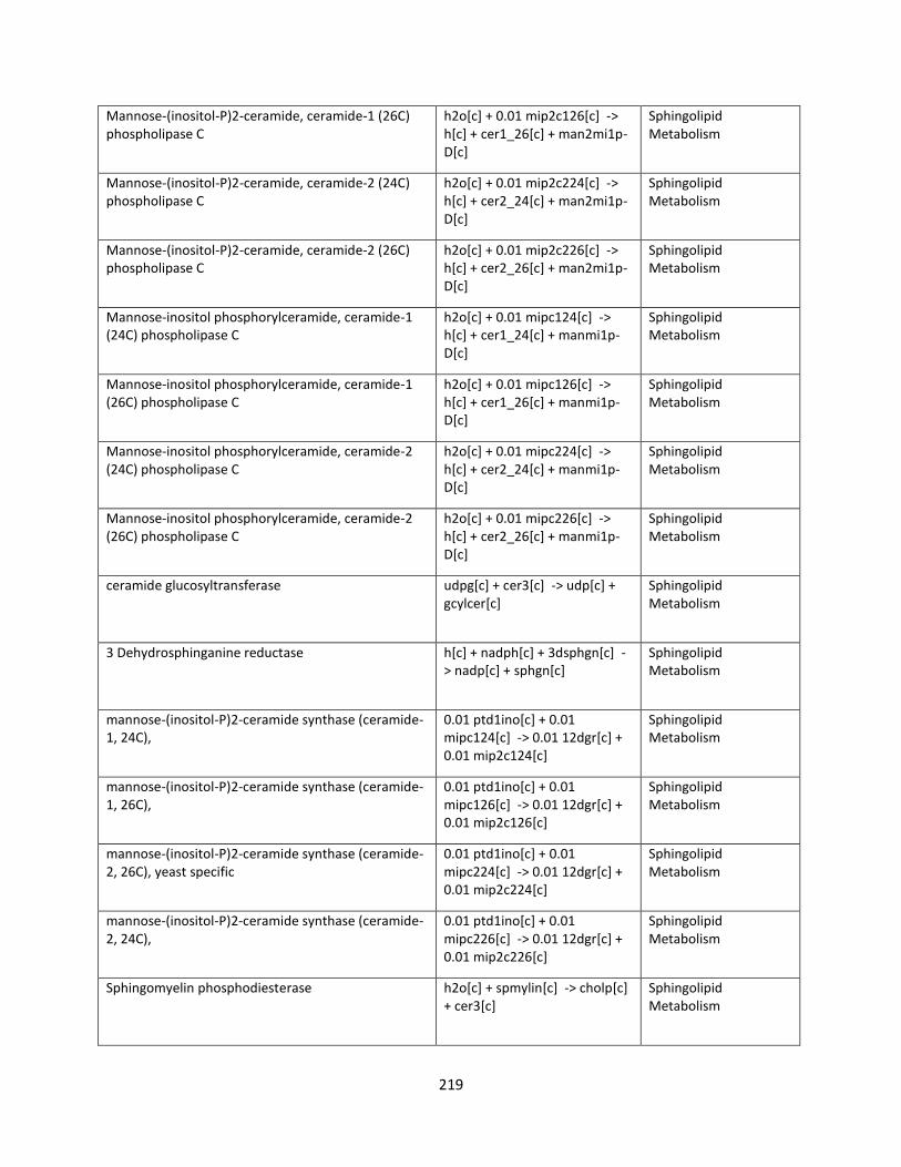
219

Mannose-(inositol-P)2-ceramide, ceramide-1 (26C) phospholipase C

h2o[c] + 0.01 mip2c126[c] -> h[c] + cer1_26[c] + man2mi1p-D[c]

Sphingolipid Metabolism

Mannose-(inositol-P)2-ceramide, ceramide-2 (24C) phospholipase C

h2o[c] + 0.01 mip2c224[c] -> h[c] + cer2_24[c] + man2mi1p-D[c]

Sphingolipid Metabolism

Mannose-(inositol-P)2-ceramide, ceramide-2 (26C) phospholipase C

h2o[c] + 0.01 mip2c226[c] -> h[c] + cer2_26[c] + man2mi1p-D[c]

Sphingolipid Metabolism

Mannose-inositol phosphorylceramide, ceramide-1 (24C) phospholipase C

h2o[c] + 0.01 mipc124[c] -> h[c] + cer1_24[c] + manmi1p-D[c]

Sphingolipid Metabolism

Mannose-inositol phosphorylceramide, ceramide-1 (26C) phospholipase C

h2o[c] + 0.01 mipc126[c] -> h[c] + cer1_26[c] + manmi1p-D[c]

Sphingolipid Metabolism

Mannose-inositol phosphorylceramide, ceramide-2 (24C) phospholipase C

h2o[c] + 0.01 mipc224[c] -> h[c] + cer2_24[c] + manmi1p-D[c]

Sphingolipid Metabolism

Mannose-inositol phosphorylceramide, ceramide-2 (26C) phospholipase C

h2o[c] + 0.01 mipc226[c] -> h[c] + cer2_26[c] + manmi1p-D[c]

Sphingolipid Metabolism

ceramide glucosyltransferase udpg[c] + cer3[c] -> udp[c] + gcylcer[c]

Sphingolipid Metabolism

3 Dehydrosphinganine reductase h[c] + nadph[c] + 3dsphgn[c] -> nadp[c] + sphgn[c]

Sphingolipid Metabolism

mannose-(inositol-P)2-ceramide synthase (ceramide-1, 24C),

0.01 ptd1ino[c] + 0.01 mipc124[c] -> 0.01 12dgr[c] + 0.01 mip2c124[c]

Sphingolipid Metabolism

mannose-(inositol-P)2-ceramide synthase (ceramide-1, 26C),

0.01 ptd1ino[c] + 0.01 mipc126[c] -> 0.01 12dgr[c] + 0.01 mip2c126[c]

Sphingolipid Metabolism

mannose-(inositol-P)2-ceramide synthase (ceramide-2, 26C), yeast specific

0.01 ptd1ino[c] + 0.01 mipc224[c] -> 0.01 12dgr[c] + 0.01 mip2c224[c]

Sphingolipid Metabolism

mannose-(inositol-P)2-ceramide synthase (ceramide-2, 24C),

0.01 ptd1ino[c] + 0.01 mipc226[c] -> 0.01 12dgr[c] + 0.01 mip2c226[c]

Sphingolipid Metabolism

Sphingomyelin phosphodiesterase h2o[c] + spmylin[c] -> cholp[c] + cer3[c]

Sphingolipid Metabolism

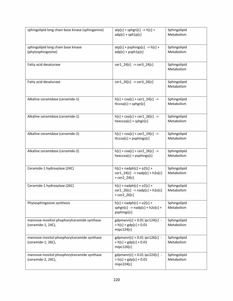
220

sphingolipid long chain base kinase (sphinganine) atp[c] + sphgn[c] -> h[c] + adp[c] + sph1p[c]

Sphingolipid Metabolism

sphingolipid long chain base kinase (phytosphingosine)

atp[c] + psphings[c] -> h[c] + adp[c] + psph1p[c]

Sphingolipid Metabolism

Fatty acid desaturase cer1_24[c] -> cer3_24[c] Sphingolipid Metabolism

Fatty acid desaturase cer1_26[c] -> cer3_26[c] Sphingolipid Metabolism

Alkaline ceramidase (ceramide-1) h[c] + coa[c] + cer1_24[c] -> ttccoa[c] + sphgn[c]

Sphingolipid Metabolism

Alkaline ceramidase (ceramide-1) h[c] + coa[c] + cer1_26[c] -> hexccoa[c] + sphgn[c]

Sphingolipid Metabolism

Alkaline ceramidase (ceramide-2) h[c] + coa[c] + cer2_24[c] -> ttccoa[c] + psphings[c]

Sphingolipid Metabolism

Alkaline ceramidase (ceramide-2) h[c] + coa[c] + cer2_26[c] -> hexccoa[c] + psphings[c]

Sphingolipid Metabolism

Ceramide-1 hydroxylase (24C) h[c] + nadph[c] + o2[c] + cer1_24[c] -> nadp[c] + h2o[c] + cer2_24[c]

Sphingolipid Metabolism

Ceramide-1 hydroxylase (26C) h[c] + nadph[c] + o2[c] + cer1_26[c] -> nadp[c] + h2o[c] + cer2_26[c]

Sphingolipid Metabolism

Phytosphingosine synthesis h[c] + nadph[c] + o2[c] + sphgn[c] -> nadp[c] + h2o[c] + psphings[c]

Sphingolipid Metabolism

mannose-inositiol phophorylceramide synthase (ceramide-1, 24C),

gdpmann[c] + 0.01 ipc124[c] -> h[c] + gdp[c] + 0.01 mipc124[c]

Sphingolipid Metabolism

mannose-inositol phosphorylceramide synthase (ceramide-1, 26C),

gdpmann[c] + 0.01 ipc126[c] -> h[c] + gdp[c] + 0.01 mipc126[c]

Sphingolipid Metabolism

mannose-inositol phosphorylceramide synthase (ceramide-2, 24C),

gdpmann[c] + 0.01 ipc224[c] -> h[c] + gdp[c] + 0.01 mipc224[c]

Sphingolipid Metabolism

221

mannose-inositol phosphorylceramide synthase (ceramide-2, 26C),

gdpmann[c] + 0.01 ipc226[c] -> h[c] + gdp[c] + 0.01 mipc226[c]

Sphingolipid Metabolism

Serine C palmitoyltransferase h[c] + ser-L[c] + pmtcoa[c] -> co2[c] + coa[c] + 3dsphgn[c]

Sphingolipid Metabolism

phytosphingosine phosphate lyase psph1p[c] -> ethamp[c] + 2hhxdal[c]

Sphingolipid Metabolism

sphinganine phosphate lyase sph1p[c] -> ethamp[c] + hxdcal[c]

Sphingolipid Metabolism

Inositol phosphorylceramide synthase (ceramide-1, 24C),

0.01 ptd1ino[c] + cer1_24[c] -> 0.01 12dgr[c] + 0.01 ipc124[c]

Sphingolipid Metabolism

Inositol phosphorylceramide synthase (ceramide-1, 26C),

0.01 ptd1ino[c] + cer1_26[c] -> 0.01 12dgr[c] + 0.01 ipc126[c]

Sphingolipid Metabolism

Inositol phosphorylceramide synthase (ceramide-2, 24C),

0.01 ptd1ino[c] + cer2_24[c] -> 0.01 12dgr[c] + 0.01 ipc224[c]

Sphingolipid Metabolism

Inositol phosphoryceramide synthase (ceramide-2, 26C),

0.01 ptd1ino[c] + cer2_26[c] -> 0.01 12dgr[c] + 0.01 ipc226[c]

Sphingolipid Metabolism

Ceramide synthase - model reaction cer3_24[c] + cer3_26[c] <=> cer3[c]

Sphingolipid Metabolism

Alpha-glucosidase h2o[c] + malt[c] -> 2 glc-D[c] Starch and sucrose metabolism

Phosphoglucomutase g1p[c] <=> g6p[c] Starch and sucrose metabolism

UTP-glucose-1-phosphate uridylyltransferase h[c] + utp[c] + g1p[c] <=> ppi[c] + udpg[c]

Starch and sucrose metabolism

C-5 sterol desaturase h[c] + nadph[c] + o2[c] + epist[c] -> nadp[c] + 2 h2o[c] + ergtrol[c]

Sterol Biosynthesis

C-s24 sterol reductase h[c] + nadph[c] + ergtetrol[c] -> nadp[c] + ergst[c]

Sterol Biosynthesis

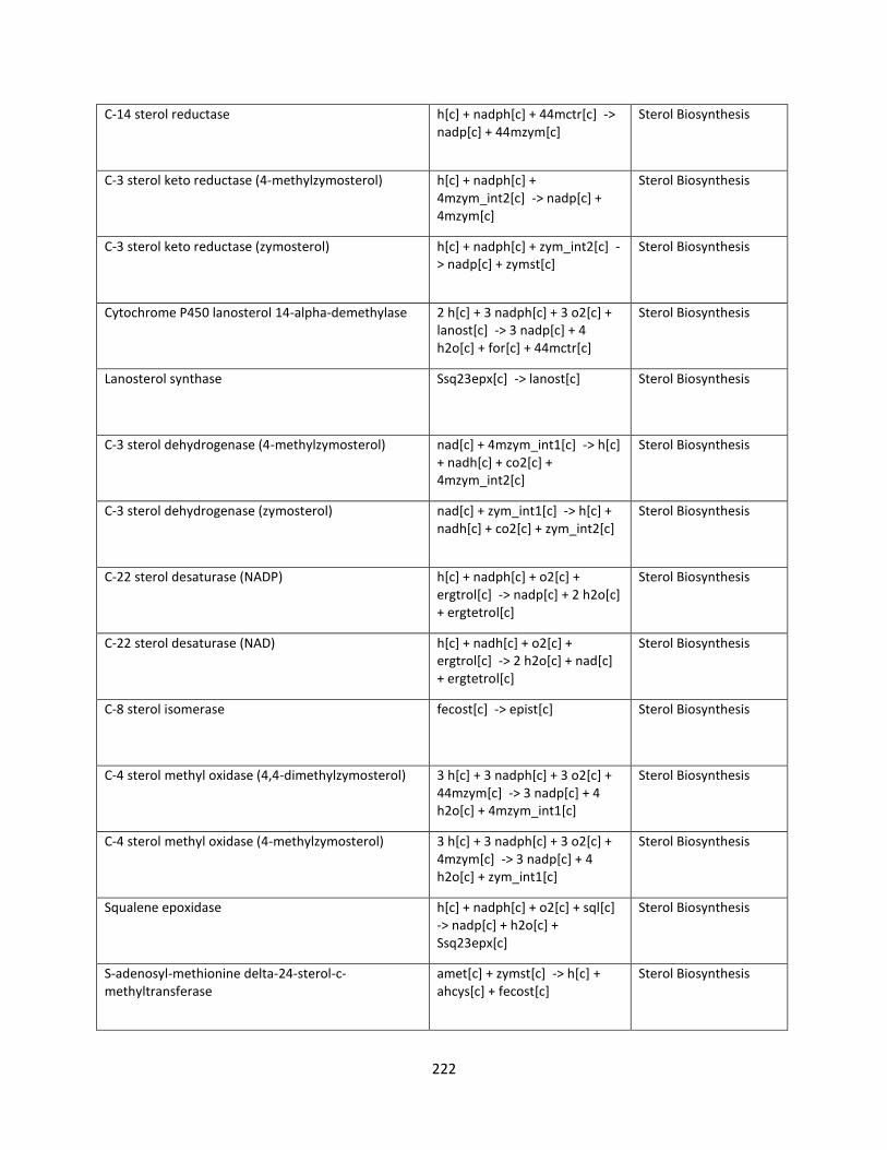
222

C-14 sterol reductase h[c] + nadph[c] + 44mctr[c] -> nadp[c] + 44mzym[c]

Sterol Biosynthesis

C-3 sterol keto reductase (4-methylzymosterol) h[c] + nadph[c] + 4mzym_int2[c] -> nadp[c] + 4mzym[c]

Sterol Biosynthesis

C-3 sterol keto reductase (zymosterol) h[c] + nadph[c] + zym_int2[c] -> nadp[c] + zymst[c]

Sterol Biosynthesis

Cytochrome P450 lanosterol 14-alpha-demethylase 2 h[c] + 3 nadph[c] + 3 o2[c] + lanost[c] -> 3 nadp[c] + 4 h2o[c] + for[c] + 44mctr[c]

Sterol Biosynthesis

Lanosterol synthase Ssq23epx[c] -> lanost[c] Sterol Biosynthesis

C-3 sterol dehydrogenase (4-methylzymosterol) nad[c] + 4mzym_int1[c] -> h[c] + nadh[c] + co2[c] + 4mzym_int2[c]

Sterol Biosynthesis

C-3 sterol dehydrogenase (zymosterol) nad[c] + zym_int1[c] -> h[c] + nadh[c] + co2[c] + zym_int2[c]

Sterol Biosynthesis

C-22 sterol desaturase (NADP) h[c] + nadph[c] + o2[c] + ergtrol[c] -> nadp[c] + 2 h2o[c] + ergtetrol[c]

Sterol Biosynthesis

C-22 sterol desaturase (NAD) h[c] + nadh[c] + o2[c] + ergtrol[c] -> 2 h2o[c] + nad[c] + ergtetrol[c]

Sterol Biosynthesis

C-8 sterol isomerase fecost[c] -> epist[c] Sterol Biosynthesis

C-4 sterol methyl oxidase (4,4-dimethylzymosterol) 3 h[c] + 3 nadph[c] + 3 o2[c] + 44mzym[c] -> 3 nadp[c] + 4 h2o[c] + 4mzym_int1[c]

Sterol Biosynthesis

C-4 sterol methyl oxidase (4-methylzymosterol) 3 h[c] + 3 nadph[c] + 3 o2[c] + 4mzym[c] -> 3 nadp[c] + 4 h2o[c] + zym_int1[c]

Sterol Biosynthesis

Squalene epoxidase h[c] + nadph[c] + o2[c] + sql[c] -> nadp[c] + h2o[c] + Ssq23epx[c]

Sterol Biosynthesis

S-adenosyl-methionine delta-24-sterol-c-methyltransferase

amet[c] + zymst[c] -> h[c] + ahcys[c] + fecost[c]

Sterol Biosynthesis

223

Squalene synthase h[c] + nadph[c] + 2 frdp[c] -> nadp[c] + 2 ppi[c] + sql[c]

Sterol Biosynthesis

Beta-glucosidase (cellobiose) h2o[e] + cellb[e] -> 2 glc-D[e] Sucrose and Starch Metabolism

Beta-glucosidase (MADG) h2o[e] + madg[e] -> glc-D[e] + meoh[e]

Sucrose and Starch Metabolism

Beta-glucosidase(MBDG) h2o[e] + mbdg[e] -> glc-D[e] + meoh[e]

Sucrose and Starch Metabolism

Glucan 1,4-alpha-glucosidase h2o[c] + glycogen[c] -> glc-D[c] Sucrose and Starch Metabolism

Endo-1,3-beta-glucan glucohydrase h2o[c] + 13BDglcn[c] -> glc-D[c]

Sucrose and Starch Metabolism

Exo-1,3-beta-glucan glucohydrase, extracellular h2o[e] + 13BDglcn[e] -> glc-D[e]

Sucrose and Starch Metabolism

Alpha-glucoside glucohydrolase h2o[c] + sucr[c] -> fru[c] + glc-D[c]

Sucrose and Starch Metabolism

1,3-beta-glucan synthase udpg[c] -> h[c] + udp[c] + 13BDglcn[c]

Sucrose and Starch Metabolism

Alpha,alpha-trehalose-phosphate synthase (UDP-forming)

udpg[c] + g6p[c] -> h[c] + udp[c] + tre6p[c]

Sucrose and Starch Metabolism

Alpha,alpha-trehalase h2o[c] + tre[c] -> 2 glc-D[c] Sucrose and Starch Metabolism

Glycogen phosphorylase pi[c] + glycogen[c] -> g1p[c] Sucrose and Starch Metabolism

Trehalose-phosphatase h2o[c] + tre6p[c] -> pi[c] + tre[c]

Sucrose and Starch Metabolism

Glycogen synthase (UDPGlc) udpg[c] -> h[c] + udp[c] + glycogen[c]

Sucrose and Starch Metabolism

224

Glycogen (starch) synthase h2o[c] + udpg[c] -> h[c] + udp[c] + 14glun[c]

Sucrose and Starch Metabolism

1,4-alpha-glucan branching enzyme 14glun[c] -> h2o[c] + glycogen[c]

Sucrose and Starch Metabolism

3',5'-bisphosphate nucleotidase pap[c] + h2o[c] -> pi[c] + amp[c]

Sulphur Metabolism

Phosphoadenylyl-sulfate reductase (thioredoxin) paps[c] + trdrd[c] -> 2 h[c] + pap[c] + trdox[c] + so3[c]

Sulphur Metabolism

Sulfate adenylyltransferase h[c] + so4[c] + atp[c] -> ppi[c] + aps[c]

Sulphur Metabolism

Sulfite reductase (NADPH) 3 nadp[c] + 3 h2o[c] + h2s[c] <=> 5 h[c] + 3 nadph[c] + so3[c]

Sulphur Metabolism

Hydroxymethylglutaryl CoA synthase h[c] + coa[c] + hmgcoa[c] <=> h2o[c] + accoa[c] + aacoa[c]

Synthesis and degradation of ketone bodies

Taurine dioxygenase akg[c] + o2[c] + taur[c] -> succ[c] + co2[c] + so3[c] + amacald[c]

Taurine and hypotaurine metabolism

Aldehyde dehydrogenase (aminoacetaldehyde, NAD) h2o[c] + nad[c] + amacald[c] -> h[c] + nadh[c] + gly[c]

Taurine and hypotaurine metabolism

Geranylgeranyltranstransferase ggdp[c] + ipdp[c] -> ppi[c] + pendp[c]

Terpenoid Backbone Synthesis

Mevalonate kinase (atp) atp[c] + mev-R[c] -> h[c] + adp[c] + 5pmev[c]

Terpenoid Backbone Synthesis

Mevalonate kinase (ctp) ctp[c] + mev-R[c] -> h[c] + cdp[c] + 5pmev[c]

Terpenoid Backbone Synthesis

Mevalonate kinase (gtp) gtp[c] + mev-R[c] -> h[c] + gdp[c] + 5pmev[c]

Terpenoid Backbone Synthesis

Mevalonate kinase (utp) utp[c] + mev-R[c] -> h[c] + udp[c] + 5pmev[c]

Terpenoid Backbone Synthesis

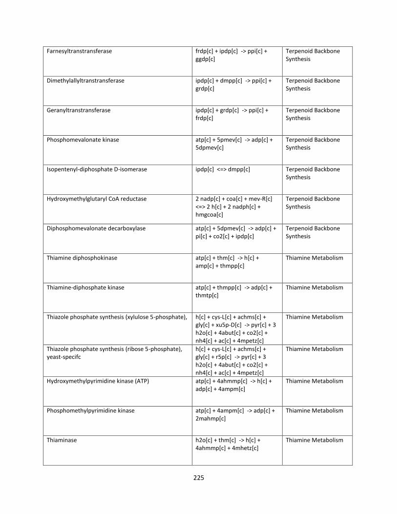
225

Farnesyltranstransferase frdp[c] + ipdp[c] -> ppi[c] + ggdp[c]

Terpenoid Backbone Synthesis

Dimethylallyltranstransferase ipdp[c] + dmpp[c] -> ppi[c] + grdp[c]

Terpenoid Backbone Synthesis

Geranyltranstransferase ipdp[c] + grdp[c] -> ppi[c] + frdp[c]

Terpenoid Backbone Synthesis

Phosphomevalonate kinase atp[c] + 5pmev[c] -> adp[c] + 5dpmev[c]

Terpenoid Backbone Synthesis

Isopentenyl-diphosphate D-isomerase ipdp[c] <=> dmpp[c] Terpenoid Backbone Synthesis

Hydroxymethylglutaryl CoA reductase 2 nadp[c] + coa[c] + mev-R[c] <=> 2 h[c] + 2 nadph[c] + hmgcoa[c]

Terpenoid Backbone Synthesis

Diphosphomevalonate decarboxylase atp[c] + 5dpmev[c] -> adp[c] + pi[c] + co2[c] + ipdp[c]

Terpenoid Backbone Synthesis

Thiamine diphosphokinase atp[c] + thm[c] -> h[c] + amp[c] + thmpp[c]

Thiamine Metabolism

Thiamine-diphosphate kinase atp[c] + thmpp[c] -> adp[c] + thmtp[c]

Thiamine Metabolism

Thiazole phosphate synthesis (xylulose 5-phosphate), h[c] + cys-L[c] + achms[c] + gly[c] + xu5p-D[c] -> pyr[c] + 3 h2o[c] + 4abut[c] + co2[c] + nh4[c] + ac[c] + 4mpetz[c]

Thiamine Metabolism

Thiazole phosphate synthesis (ribose 5-phosphate), yeast-specifc

h[c] + cys-L[c] + achms[c] + gly[c] + r5p[c] -> pyr[c] + 3 h2o[c] + 4abut[c] + co2[c] + nh4[c] + ac[c] + 4mpetz[c]

Thiamine Metabolism

Hydroxymethylpyrimidine kinase (ATP) atp[c] + 4ahmmp[c] -> h[c] + adp[c] + 4ampm[c]

Thiamine Metabolism

Phosphomethylpyrimidine kinase atp[c] + 4ampm[c] -> adp[c] + 2mahmp[c]

Thiamine Metabolism

Thiaminase h2o[c] + thm[c] -> h[c] + 4ahmmp[c] + 4mhetz[c]

Thiamine Metabolism

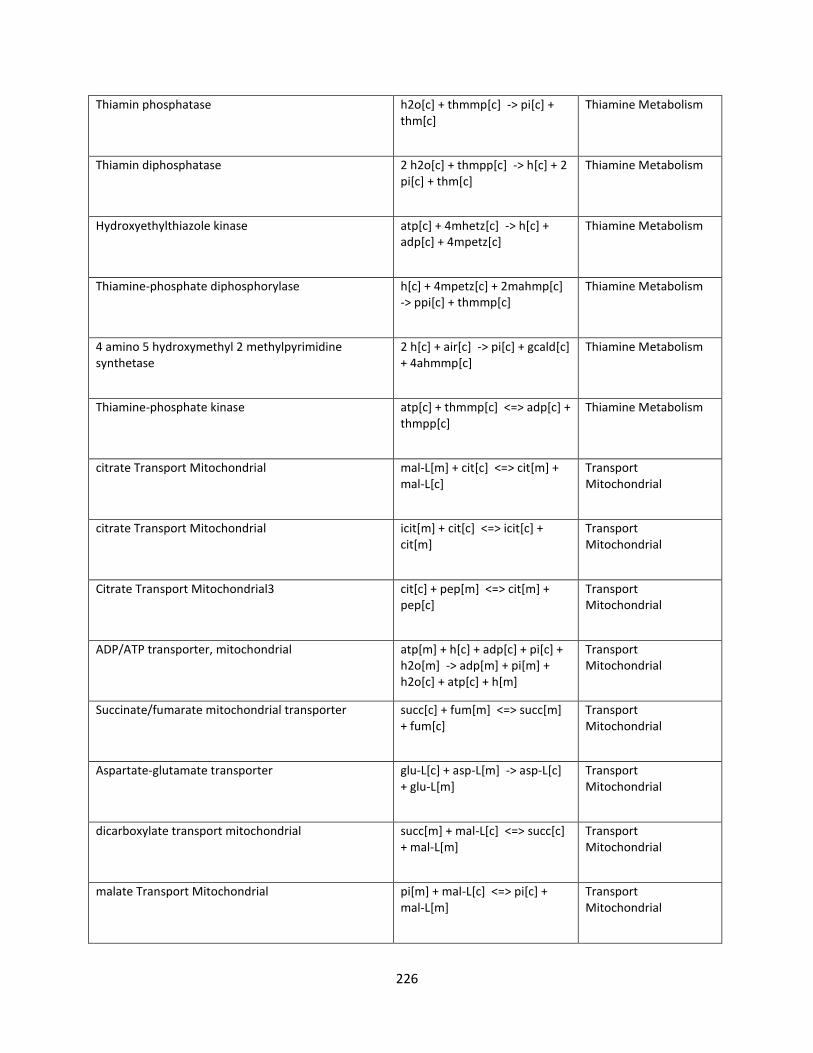
226

Thiamin phosphatase h2o[c] + thmmp[c] -> pi[c] + thm[c]

Thiamine Metabolism

Thiamin diphosphatase 2 h2o[c] + thmpp[c] -> h[c] + 2 pi[c] + thm[c]

Thiamine Metabolism

Hydroxyethylthiazole kinase atp[c] + 4mhetz[c] -> h[c] + adp[c] + 4mpetz[c]

Thiamine Metabolism

Thiamine-phosphate diphosphorylase h[c] + 4mpetz[c] + 2mahmp[c] -> ppi[c] + thmmp[c]

Thiamine Metabolism

4 amino 5 hydroxymethyl 2 methylpyrimidine synthetase

2 h[c] + air[c] -> pi[c] + gcald[c] + 4ahmmp[c]

Thiamine Metabolism

Thiamine-phosphate kinase atp[c] + thmmp[c] <=> adp[c] + thmpp[c]

Thiamine Metabolism

citrate Transport Mitochondrial mal-L[m] + cit[c] <=> cit[m] + mal-L[c]

Transport Mitochondrial

citrate Transport Mitochondrial icit[m] + cit[c] <=> icit[c] + cit[m]

Transport Mitochondrial

Citrate Transport Mitochondrial3 cit[c] + pep[m] <=> cit[m] + pep[c]

Transport Mitochondrial

ADP/ATP transporter, mitochondrial atp[m] + h[c] + adp[c] + pi[c] + h2o[m] -> adp[m] + pi[m] + h2o[c] + atp[c] + h[m]

Transport Mitochondrial

Succinate/fumarate mitochondrial transporter succ[c] + fum[m] <=> succ[m] + fum[c]

Transport Mitochondrial

Aspartate-glutamate transporter glu-L[c] + asp-L[m] -> asp-L[c] + glu-L[m]

Transport Mitochondrial

dicarboxylate transport mitochondrial succ[m] + mal-L[c] <=> succ[c] + mal-L[m]

Transport Mitochondrial

malate Transport Mitochondrial pi[m] + mal-L[c] <=> pi[c] + mal-L[m]

Transport Mitochondrial

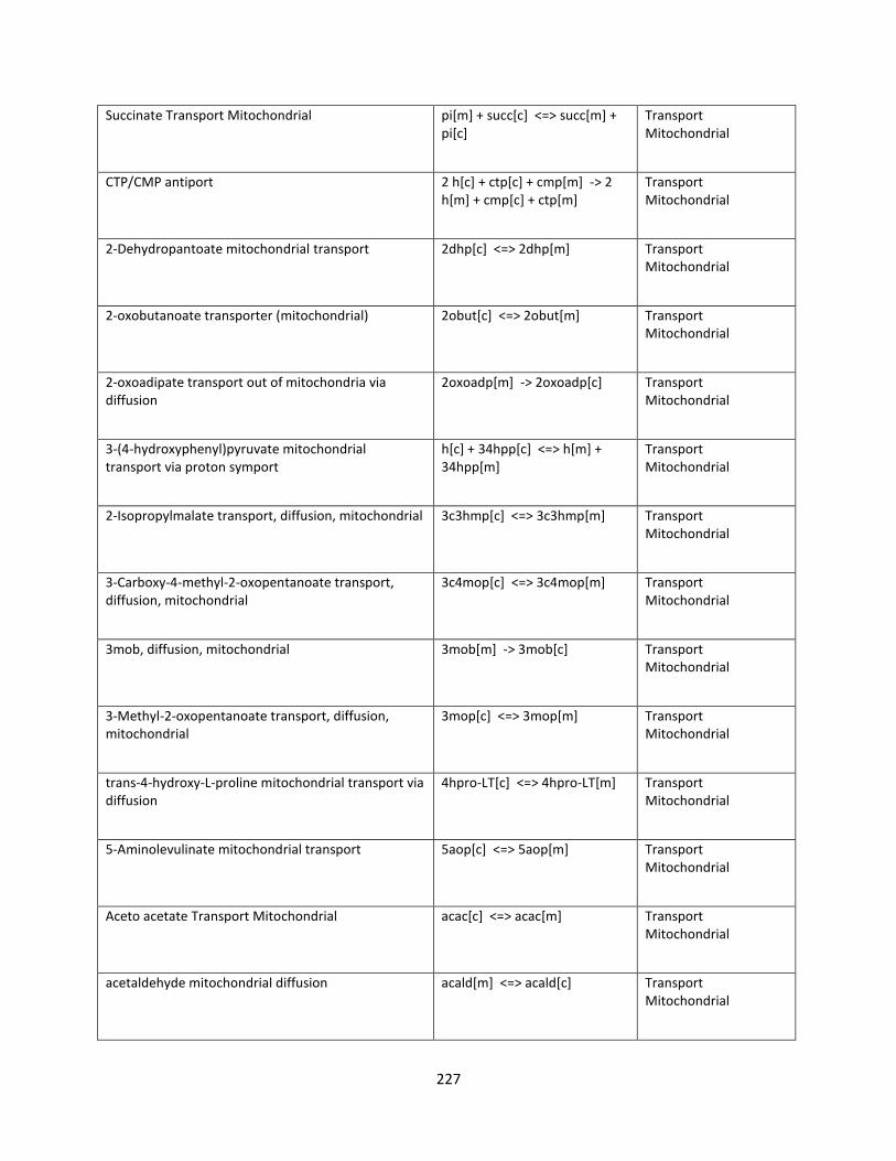
227

Succinate Transport Mitochondrial pi[m] + succ[c] <=> succ[m] + pi[c]

Transport Mitochondrial

CTP/CMP antiport 2 h[c] + ctp[c] + cmp[m] -> 2 h[m] + cmp[c] + ctp[m]

Transport Mitochondrial

2-Dehydropantoate mitochondrial transport 2dhp[c] <=> 2dhp[m] Transport Mitochondrial

2-oxobutanoate transporter (mitochondrial) 2obut[c] <=> 2obut[m] Transport Mitochondrial

2-oxoadipate transport out of mitochondria via diffusion

2oxoadp[m] -> 2oxoadp[c] Transport Mitochondrial

3-(4-hydroxyphenyl)pyruvate mitochondrial transport via proton symport

h[c] + 34hpp[c] <=> h[m] + 34hpp[m]

Transport Mitochondrial

2-Isopropylmalate transport, diffusion, mitochondrial 3c3hmp[c] <=> 3c3hmp[m] Transport Mitochondrial

3-Carboxy-4-methyl-2-oxopentanoate transport, diffusion, mitochondrial

3c4mop[c] <=> 3c4mop[m] Transport Mitochondrial

3mob, diffusion, mitochondrial 3mob[m] -> 3mob[c] Transport Mitochondrial

3-Methyl-2-oxopentanoate transport, diffusion, mitochondrial

3mop[c] <=> 3mop[m] Transport Mitochondrial

trans-4-hydroxy-L-proline mitochondrial transport via diffusion

4hpro-LT[c] <=> 4hpro-LT[m] Transport Mitochondrial

5-Aminolevulinate mitochondrial transport 5aop[c] <=> 5aop[m] Transport Mitochondrial

Aceto acetate Transport Mitochondrial acac[c] <=> acac[m] Transport Mitochondrial

acetaldehyde mitochondrial diffusion acald[m] <=> acald[c] Transport Mitochondrial

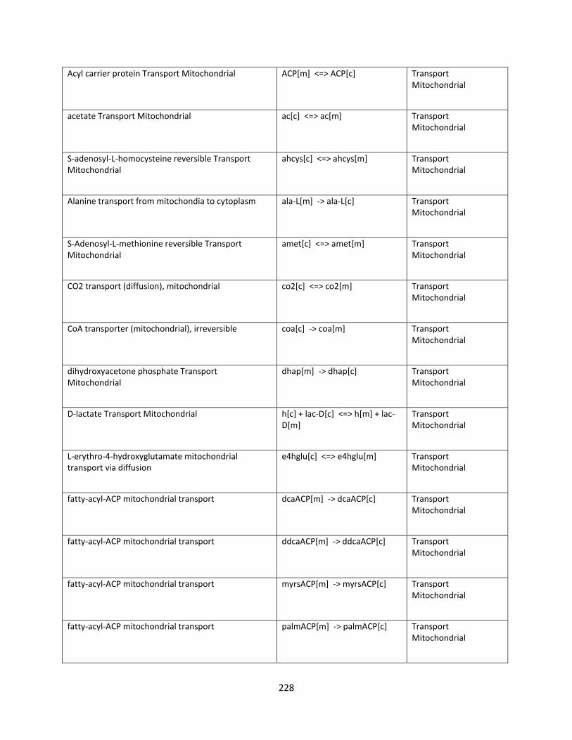
228

Acyl carrier protein Transport Mitochondrial ACP[m] <=> ACP[c] Transport Mitochondrial

acetate Transport Mitochondrial ac[c] <=> ac[m] Transport Mitochondrial

S-adenosyl-L-homocysteine reversible Transport Mitochondrial

ahcys[c] <=> ahcys[m] Transport Mitochondrial

Alanine transport from mitochondia to cytoplasm ala-L[m] -> ala-L[c] Transport Mitochondrial

S-Adenosyl-L-methionine reversible Transport Mitochondrial

amet[c] <=> amet[m] Transport Mitochondrial

CO2 transport (diffusion), mitochondrial co2[c] <=> co2[m] Transport Mitochondrial

CoA transporter (mitochondrial), irreversible coa[c] -> coa[m] Transport Mitochondrial

dihydroxyacetone phosphate Transport Mitochondrial

dhap[m] -> dhap[c] Transport Mitochondrial

D-lactate Transport Mitochondrial h[c] + lac-D[c] <=> h[m] + lac-D[m]

Transport Mitochondrial

L-erythro-4-hydroxyglutamate mitochondrial transport via diffusion

e4hglu[c] <=> e4hglu[m] Transport Mitochondrial

fatty-acyl-ACP mitochondrial transport dcaACP[m] -> dcaACP[c] Transport Mitochondrial

fatty-acyl-ACP mitochondrial transport ddcaACP[m] -> ddcaACP[c] Transport Mitochondrial

fatty-acyl-ACP mitochondrial transport myrsACP[m] -> myrsACP[c] Transport Mitochondrial

fatty-acyl-ACP mitochondrial transport palmACP[m] -> palmACP[c] Transport Mitochondrial

229

fatty-acyl-ACP mitochondrial transport hdceaACP[m] -> hdceaACP[c] Transport Mitochondrial

fatty-acyl-ACP mitochondrial transport hepdcaACP[m] -> hepdcaACP[c]

Transport Mitochondrial

fatty-acyl-ACP mitochondrial transport hepdceaACP[m] -> hepdceaACP[c]

Transport Mitochondrial

fatty-acyl-ACP mitochondrial transport ocdcaACP[m] -> ocdcaACP[c] Transport Mitochondrial

fatty-acyl-ACP mitochondrial transport ocdceaACP[m] -> ocdceaACP[c]

Transport Mitochondrial

fatty-acyl-ACP mitochondrial transport ocdcyaACP[m] -> ocdcyaACP[c]

Transport Mitochondrial

fatty-acyl-ACP mitochondrial transport ocdctaACP[m] -> ocdctaACP[c] Transport Mitochondrial

fatty-acyl-ACP mitochondrial transport eicosaACP[m] -> eicosaACP[c] Transport Mitochondrial

fatty-acyl-ACP mitochondrial transport eicosapenACP[m] -> eicosapenACP[c]

Transport Mitochondrial

fatty-acyl-ACP mitochondrial transport docosaACP[m] -> docosaACP[c]

Transport Mitochondrial

fatty-acyl-ACP mitochondrial transport ttcACP[m] -> ttcACP[c] Transport Mitochondrial

fatty-acyl-ACP mitochondrial transport hexcACP[m] -> hexcACP[c] Transport Mitochondrial

fatty-acyl-ACP mitochondrial transport hexaACP[m] -> hexaACP[c] Transport Mitochondrial

fatty-acyl-ACP mitochondrial transport octaACP[m] -> octaACP[c] Transport Mitochondrial

230

iron (II) uptake (mitochondrial) fe2[c] -> fe2[m] Transport Mitochondrial

iron (II) transport fe2[m] -> fe2[c] Transport Mitochondrial

formate mitochondrial transport for[m] -> for[c] Transport Mitochondrial

farnesyl diphosphate transport (mitochondrial) frdp[c] <=> frdp[m] Transport Mitochondrial

glycerol-3-phosphate shuttle glyc3p[c] -> glyc3p[m] Transport Mitochondrial

glycine mitochondrial transport via proton symport h[c] + gly[c] <=> h[m] + gly[m] Transport Mitochondrial

H2O Transport Mitochondrial h2o[c] <=> h2o[m] Transport Mitochondrial

Hydroxyisobutyrate Transport Mitochondrial hibut[m] <=> hibut[c] Transport Mitochondrial

Isobutyryl coA transport Mitochondrial ibcoa[m] <=> ibcoa[c] Transport Mitochondrial

Isoleucine transport from mitochondria to cytosol ile-L[m] -> ile-L[c] Transport Mitochondrial

Isopentenyl diphosphate Transport Mitochondrial ipdp[c] <=> ipdp[m] Transport Mitochondrial

Isovaleryl coA transport Mitochondrial ivcoa[m] <=> ivcoa[c] Transport Mitochondrial

L-lactate Transport Mitochondrial h[c] + lac-L[c] <=> h[m] + lac-L[m]

Transport Mitochondrial

NH3 mitochondrial transport nh4[c] <=> nh4[m] Transport Mitochondrial

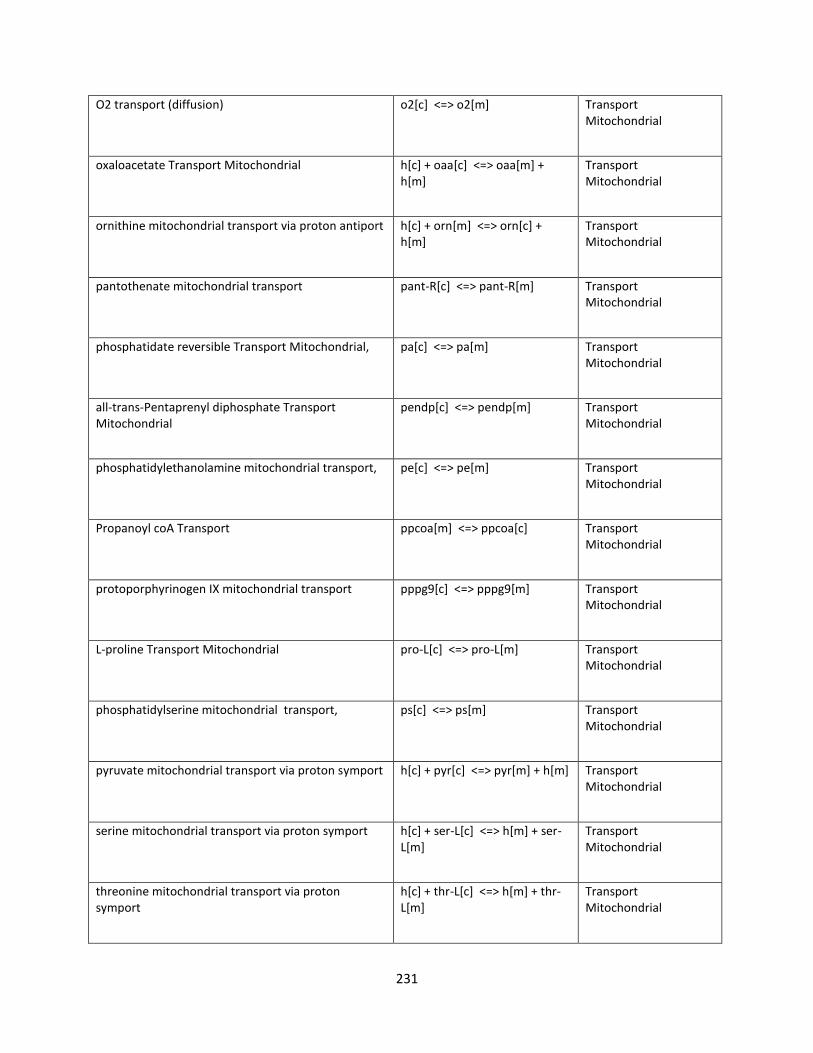
231

O2 transport (diffusion) o2[c] <=> o2[m] Transport Mitochondrial

oxaloacetate Transport Mitochondrial h[c] + oaa[c] <=> oaa[m] + h[m]

Transport Mitochondrial

ornithine mitochondrial transport via proton antiport h[c] + orn[m] <=> orn[c] + h[m]

Transport Mitochondrial

pantothenate mitochondrial transport pant-R[c] <=> pant-R[m] Transport Mitochondrial

phosphatidate reversible Transport Mitochondrial, pa[c] <=> pa[m] Transport Mitochondrial

all-trans-Pentaprenyl diphosphate Transport Mitochondrial

pendp[c] <=> pendp[m] Transport Mitochondrial

phosphatidylethanolamine mitochondrial transport, pe[c] <=> pe[m] Transport Mitochondrial

Propanoyl coA Transport ppcoa[m] <=> ppcoa[c] Transport Mitochondrial

protoporphyrinogen IX mitochondrial transport pppg9[c] <=> pppg9[m] Transport Mitochondrial

L-proline Transport Mitochondrial pro-L[c] <=> pro-L[m] Transport Mitochondrial

phosphatidylserine mitochondrial transport, ps[c] <=> ps[m] Transport Mitochondrial

pyruvate mitochondrial transport via proton symport h[c] + pyr[c] <=> pyr[m] + h[m] Transport Mitochondrial

serine mitochondrial transport via proton symport h[c] + ser-L[c] <=> h[m] + ser-L[m]

Transport Mitochondrial

threonine mitochondrial transport via proton symport

h[c] + thr-L[c] <=> h[m] + thr-L[m]

Transport Mitochondrial

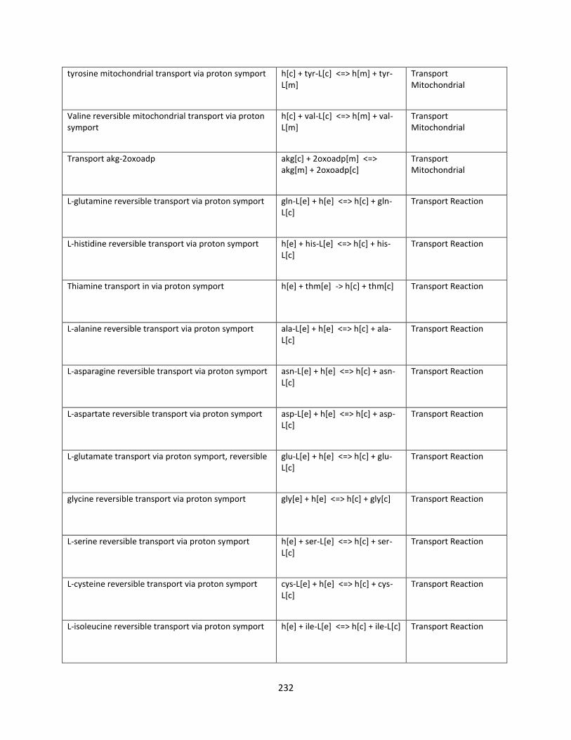
232

tyrosine mitochondrial transport via proton symport h[c] + tyr-L[c] <=> h[m] + tyr-L[m]

Transport Mitochondrial

Valine reversible mitochondrial transport via proton symport

h[c] + val-L[c] <=> h[m] + val-L[m]

Transport Mitochondrial

Transport akg-2oxoadp akg[c] + 2oxoadp[m] <=> akg[m] + 2oxoadp[c]

Transport Mitochondrial

L-glutamine reversible transport via proton symport gln-L[e] + h[e] <=> h[c] + gln-L[c]

Transport Reaction

L-histidine reversible transport via proton symport h[e] + his-L[e] <=> h[c] + his-L[c]

Transport Reaction

Thiamine transport in via proton symport h[e] + thm[e] -> h[c] + thm[c] Transport Reaction

L-alanine reversible transport via proton symport ala-L[e] + h[e] <=> h[c] + ala-L[c]

Transport Reaction

L-asparagine reversible transport via proton symport asn-L[e] + h[e] <=> h[c] + asn-L[c]

Transport Reaction

L-aspartate reversible transport via proton symport asp-L[e] + h[e] <=> h[c] + asp-L[c]

Transport Reaction

L-glutamate transport via proton symport, reversible glu-L[e] + h[e] <=> h[c] + glu-L[c]

Transport Reaction

glycine reversible transport via proton symport gly[e] + h[e] <=> h[c] + gly[c] Transport Reaction

L-serine reversible transport via proton symport h[e] + ser-L[e] <=> h[c] + ser-L[c]

Transport Reaction

L-cysteine reversible transport via proton symport cys-L[e] + h[e] <=> h[c] + cys-L[c]

Transport Reaction

L-isoleucine reversible transport via proton symport h[e] + ile-L[e] <=> h[c] + ile-L[c] Transport Reaction

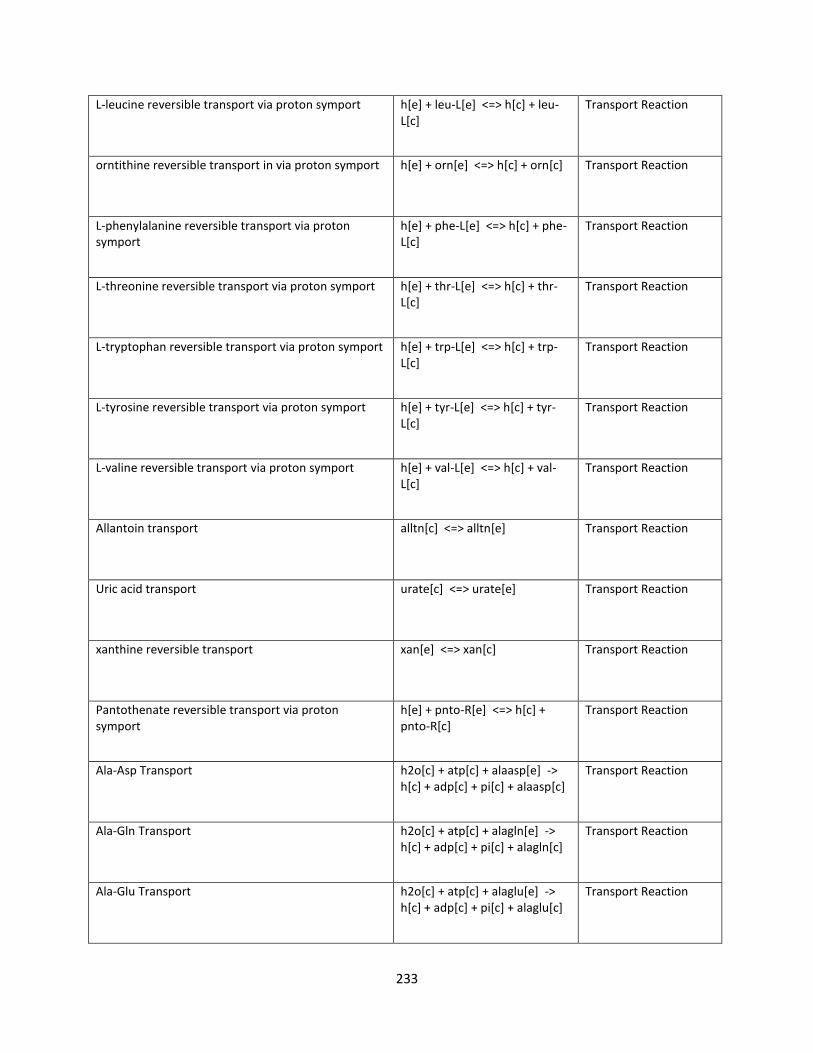
233

L-leucine reversible transport via proton symport h[e] + leu-L[e] <=> h[c] + leu-L[c]

Transport Reaction

orntithine reversible transport in via proton symport h[e] + orn[e] <=> h[c] + orn[c] Transport Reaction

L-phenylalanine reversible transport via proton symport

h[e] + phe-L[e] <=> h[c] + phe-L[c]

Transport Reaction

L-threonine reversible transport via proton symport h[e] + thr-L[e] <=> h[c] + thr-L[c]

Transport Reaction

L-tryptophan reversible transport via proton symport h[e] + trp-L[e] <=> h[c] + trp-L[c]

Transport Reaction

L-tyrosine reversible transport via proton symport h[e] + tyr-L[e] <=> h[c] + tyr-L[c]

Transport Reaction

L-valine reversible transport via proton symport h[e] + val-L[e] <=> h[c] + val-L[c]

Transport Reaction

Allantoin transport alltn[c] <=> alltn[e] Transport Reaction

Uric acid transport urate[c] <=> urate[e] Transport Reaction

xanthine reversible transport xan[e] <=> xan[c] Transport Reaction

Pantothenate reversible transport via proton symport

h[e] + pnto-R[e] <=> h[c] + pnto-R[c]

Transport Reaction

Ala-Asp Transport h2o[c] + atp[c] + alaasp[e] -> h[c] + adp[c] + pi[c] + alaasp[c]

Transport Reaction

Ala-Gln Transport h2o[c] + atp[c] + alagln[e] -> h[c] + adp[c] + pi[c] + alagln[c]

Transport Reaction

Ala-Glu Transport h2o[c] + atp[c] + alaglu[e] -> h[c] + adp[c] + pi[c] + alaglu[c]

Transport Reaction

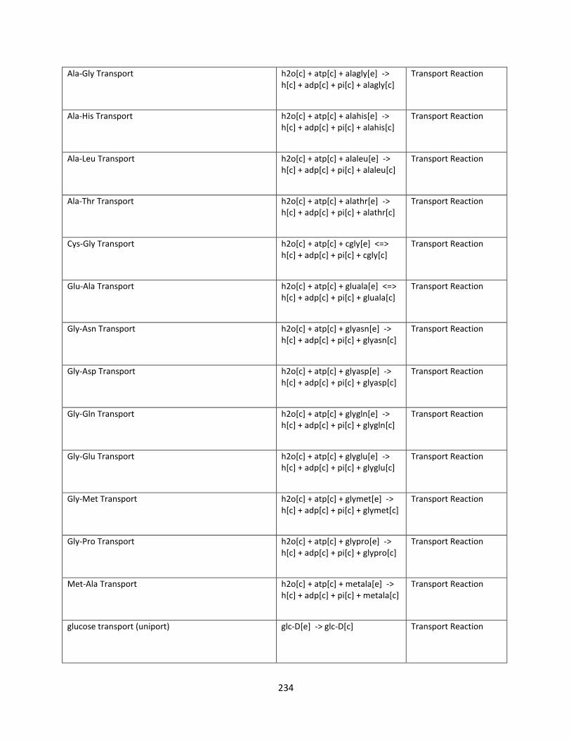
234

Ala-Gly Transport h2o[c] + atp[c] + alagly[e] -> h[c] + adp[c] + pi[c] + alagly[c]

Transport Reaction

Ala-His Transport h2o[c] + atp[c] + alahis[e] -> h[c] + adp[c] + pi[c] + alahis[c]

Transport Reaction

Ala-Leu Transport h2o[c] + atp[c] + alaleu[e] -> h[c] + adp[c] + pi[c] + alaleu[c]

Transport Reaction

Ala-Thr Transport h2o[c] + atp[c] + alathr[e] -> h[c] + adp[c] + pi[c] + alathr[c]

Transport Reaction

Cys-Gly Transport h2o[c] + atp[c] + cgly[e] <=> h[c] + adp[c] + pi[c] + cgly[c]

Transport Reaction

Glu-Ala Transport h2o[c] + atp[c] + gluala[e] <=> h[c] + adp[c] + pi[c] + gluala[c]

Transport Reaction

Gly-Asn Transport h2o[c] + atp[c] + glyasn[e] -> h[c] + adp[c] + pi[c] + glyasn[c]

Transport Reaction

Gly-Asp Transport h2o[c] + atp[c] + glyasp[e] -> h[c] + adp[c] + pi[c] + glyasp[c]

Transport Reaction

Gly-Gln Transport h2o[c] + atp[c] + glygln[e] -> h[c] + adp[c] + pi[c] + glygln[c]

Transport Reaction

Gly-Glu Transport h2o[c] + atp[c] + glyglu[e] -> h[c] + adp[c] + pi[c] + glyglu[c]

Transport Reaction

Gly-Met Transport h2o[c] + atp[c] + glymet[e] -> h[c] + adp[c] + pi[c] + glymet[c]

Transport Reaction

Gly-Pro Transport h2o[c] + atp[c] + glypro[e] -> h[c] + adp[c] + pi[c] + glypro[c]

Transport Reaction

Met-Ala Transport h2o[c] + atp[c] + metala[e] -> h[c] + adp[c] + pi[c] + metala[c]

Transport Reaction

glucose transport (uniport) glc-D[e] -> glc-D[c] Transport Reaction

235

Lactose transport in via proton symport h[e] + lact[e] -> h[c] + lact[c] Transport Reaction

4-aminobutyrate reversible transport in via proton symport

4abut[e] + h[e] <=> h[c] + 4abut[c]

Transport Reaction

D-xylose reversible transport h[e] + xyl-D[e] <=> h[c] + xyl-D[c]

Transport Reaction

maltose transport in via proton symport h[e] + malt[e] -> h[c] + malt[c] Transport Reaction

D-fructose transport in via proton symport fru[e] + h[e] -> h[c] + fru[c] Transport Reaction

adenine transport in via proton symport ade[e] + h[e] -> h[c] + ade[c] Transport Reaction

L-proline reversible transport via proton symport h[e] + pro-L[e] <=> h[c] + pro-L[c]

Transport Reaction

urea reversible transport via proton symport (2 H+) 2 h[e] + urea[e] <=> 2 h[c] + urea[c]

Transport Reaction

D-galactose transport in via proton symport gal[e] + h[e] -> h[c] + gal[c] Transport Reaction

cytidine transport in via proton symport cytd[e] + h[e] -> h[c] + cytd[c] Transport Reaction

guanine reversible transport via proton symport gua[e] + h[e] -> h[c] + gua[c] Transport Reaction

Nicotinic acid transport nac[e] <=> nac[c] Transport Reaction

phosphate reversible transport via symport h[e] + pi[e] <=> h[c] + pi[c] Transport Reaction

glycerol transport via symport glyc[e] + h[e] -> h[c] + glyc[c] Transport Reaction

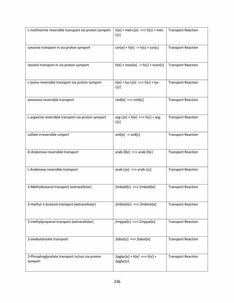
236

L-methionine reversible transport via proton symport h[e] + met-L[e] <=> h[c] + met-L[c]

Transport Reaction

cytosine transport in via proton symport csn[e] + h[e] -> h[c] + csn[c] Transport Reaction

inositol transport in via proton symport h[e] + inost[e] -> h[c] + inost[c] Transport Reaction

L-lysine reversible transport via proton symport h[e] + lys-L[e] <=> h[c] + lys-L[c]

Transport Reaction

ammonia reversible transport nh4[e] <=> nh4[c] Transport Reaction

L-arganine reversible transport via proton symport arg-L[e] + h[e] <=> h[c] + arg-L[c]

Transport Reaction

sulfate irreversible uniport so4[e] -> so4[c] Transport Reaction

D-Arabinose reversible transport arab-D[e] <=> arab-D[c] Transport Reaction

L-Arabinose reversible transport arab-L[e] <=> arab-L[c] Transport Reaction

2-Methylbutanal transport (extracellular) 2mbald[c] <=> 2mbald[e] Transport Reaction

2-methyl-1-butanol transport (extracellular) 2mbtoh[c] <=> 2mbtoh[e] Transport Reaction

2-methylpropanal transport (extracellular) 2mppal[c] <=> 2mppal[e] Transport Reaction

2-oxobutanoate transport 2obut[c] <=> 2obut[e] Transport Reaction

2-Phosphoglycolate transport in/out via proton symport

2pglyc[e] + h[e] <=> h[c] + 2pglyc[c]

Transport Reaction

237

D-Glycerate 2-phosphate transport in/out via proton symport

2pg[e] + h[e] -> h[c] + 2pg[c] Transport Reaction

2-phenylethanol reversible transport 2phetoh[e] <=> 2phetoh[c] Transport Reaction

2-Isopropylmalate transport, diffusion 3c3hmp[c] <=> 3c3hmp[e] Transport Reaction

3-methylbutanal transport (extracellular) 3mbald[c] <=> 3mbald[e] Transport Reaction

3mop reversible trasport 3mop[e] <=> 3mop[c] Transport Reaction

3-Phospho-D-glycerate transport in/out via proton symport

3pg[e] + h[e] -> h[c] + 3pg[c] Transport Reaction

4-Aminobenzoate mitochondrial transport via diffusion

4abz[c] <=> 4abz[e] Transport Reaction

hydroxyproline transport 4hpro-LT[c] <=> 4hpro-LT[e] Transport Reaction

5-Aminolevulinate transport in via proton symport 5aop[e] + h[e] -> h[c] + 5aop[c] Transport Reaction

6-Phospho-D-gluconate transport in/out via proton symport

6pgc[e] + h[e] <=> h[c] + 6pgc[c]

Transport Reaction

8-Amino-7-oxononanoate reversible transport via proton symport

8aonn[e] + h[e] <=> h[c] + 8aonn[c]

Transport Reaction

Acetoacetate transport acac[c] <=> acac[e] Transport Reaction

acetaldehyde reversible transport acald[e] <=> acald[c] Transport Reaction

Acetamide transport acetm[c] <=> acetm[e] Transport Reaction

238

N-Acetyl Glucosamine reversible transport acgam[e] <=> acgam[c] Transport Reaction

acetate transporter ac[e] <=> ac[c] Transport Reaction

adenosine transport in via proton symport adn[e] + h[e] -> h[c] + adn[c] Transport Reaction

Agmatine transport agm[c] <=> agm[e] Transport Reaction

2-oxoglutarate reversible transport via symport akg[e] + h[e] <=> h[c] + akg[c] Transport Reaction

D-Alanine reversible transport ala-D[e] <=> ala-D[c] Transport Reaction

S-adenosyl-L-methionine transport in via proton symport

amet[e] + h[e] -> h[c] + amet[c]

Transport Reaction

AMP transport in/out via proton symport amp[e] + h[e] <=> h[c] + amp[c]

Transport Reaction

D-Arabinitol reversible transport abt-D[e] <=> abt-D[c] Transport Reaction

L-Arabinitol reversible transport abt-L[e] <=> abt-L[c] Transport Reaction

(R,R)-butanediol transport btd-RR[c] <=> btd-RR[e] Transport Reaction

Biotin uptake btn[e] + h[e] -> h[c] + btn[c] Transport Reaction

Methanethiol Transport ch4s[e] <=> ch4s[c] Transport Reaction

choline transport via proton symport chol[e] + h[e] <=> h[c] + chol[c]

Transport Reaction

239

L-Citruline transport citr-L[c] <=> citr-L[e] Transport Reaction

citrate reversible transport via symport cit[e] + h[e] <=> h[c] + cit[c] Transport Reaction

CMP transport in/out via proton symport cmp[e] + h[e] <=> h[c] + cmp[c]

Transport Reaction

CO2 transporter via diffusion co2[e] <=> co2[c] Transport Reaction

Cystathione Transport cyst-L[e] <=> cyst-L[c] Transport Reaction

deoxyadenosine transport in via proton symport dad-2[e] + h[e] -> h[c] + dad-2[c]

Transport Reaction

7,8-Diaminononanoate reversible transport via proton symport

dann[e] + h[e] <=> h[c] + dann[c]

Transport Reaction

Decanoate (n-C10:0), Transport dca[e] <=> dca[c] Transport Reaction

deoxycytidine transport in via proton symport dcyt[e] + h[e] -> h[c] + dcyt[c] Transport Reaction

Dodecanoate (n-C12:0), Transport ddca[e] <=> ddca[c] Transport Reaction

deoxyguanosine transport in via proton symport dgsn[e] + h[e] -> h[c] + dgsn[c] Transport Reaction

Dihydroxy acetone transport dha[c] <=> dha[e] Transport Reaction

deoxyinosine transport in via proton symport din[e] + h[e] -> h[c] + din[c] Transport Reaction

D-lactate transport via proton symport h[e] + lac-D[e] <=> h[c] + lac-D[c]

Transport Reaction

240

Docosanoic acid, Transport docosa[e] <=> docosa[c] Transport Reaction

Thymidine 5 Phosphate Transport dtmp[c] <=> dtmp[e] Transport Reaction

dTTP reversible uniport dttp[e] <=> dttp[c] Transport Reaction

deoxyuridine transport in via proton symport duri[e] + h[e] -> h[c] + duri[c] Transport Reaction

Eicosapentaenoate, Transport eicosapen[e] <=> eicosapen[c] Transport Reaction

episterol reversible transport epist[e] <=> epist[c] Transport Reaction

ergosterol reversible transport ergst[e] <=> ergst[c] Transport Reaction

ethanolamine transport via diffusion (extracellular) etha[e] <=> etha[c] Transport Reaction

ethanol reversible transport etoh[e] <=> etoh[c] Transport Reaction

Lactose Exchange lact[e] <=> Transport Reaction

Fructose-6-phosphate transport via phosphate antiport

2 pi[c] + f6p[e] -> f6p[c] + 2 pi[e]

Transport Reaction

iron (II) transport fe2[e] -> fe2[c] Transport Reaction

fecosterol reversible transport fecost[e] <=> fecost[c] Transport Reaction

formate transport via diffusion for[e] <=> for[c] Transport Reaction

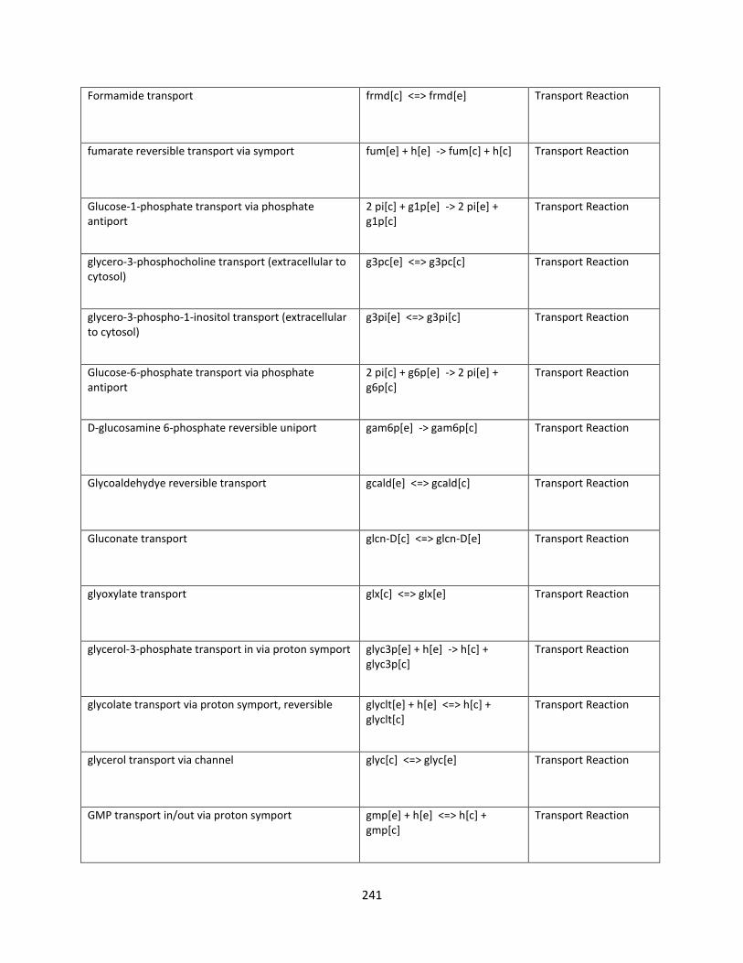
241

Formamide transport frmd[c] <=> frmd[e] Transport Reaction

fumarate reversible transport via symport fum[e] + h[e] -> fum[c] + h[c] Transport Reaction

Glucose-1-phosphate transport via phosphate antiport

2 pi[c] + g1p[e] -> 2 pi[e] + g1p[c]

Transport Reaction

glycero-3-phosphocholine transport (extracellular to cytosol)

g3pc[e] <=> g3pc[c] Transport Reaction

glycero-3-phospho-1-inositol transport (extracellular to cytosol)

g3pi[e] <=> g3pi[c] Transport Reaction

Glucose-6-phosphate transport via phosphate antiport

2 pi[c] + g6p[e] -> 2 pi[e] + g6p[c]

Transport Reaction

D-glucosamine 6-phosphate reversible uniport gam6p[e] -> gam6p[c] Transport Reaction

Glycoaldehydye reversible transport gcald[e] <=> gcald[c] Transport Reaction

Gluconate transport glcn-D[c] <=> glcn-D[e] Transport Reaction

glyoxylate transport glx[c] <=> glx[e] Transport Reaction

glycerol-3-phosphate transport in via proton symport glyc3p[e] + h[e] -> h[c] + glyc3p[c]

Transport Reaction

glycolate transport via proton symport, reversible glyclt[e] + h[e] <=> h[c] + glyclt[c]

Transport Reaction

glycerol transport via channel glyc[c] <=> glyc[e] Transport Reaction

GMP transport in/out via proton symport gmp[e] + h[e] <=> h[c] + gmp[c]

Transport Reaction

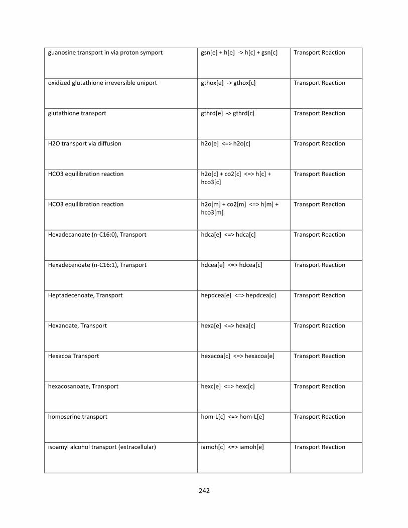
242

guanosine transport in via proton symport gsn[e] + h[e] -> h[c] + gsn[c] Transport Reaction

oxidized glutathione irreversible uniport gthox[e] -> gthox[c] Transport Reaction

glutathione transport gthrd[e] -> gthrd[c] Transport Reaction

H2O transport via diffusion h2o[e] <=> h2o[c] Transport Reaction

HCO3 equilibration reaction h2o[c] + co2[c] <=> h[c] + hco3[c]

Transport Reaction

HCO3 equilibration reaction h2o[m] + co2[m] <=> h[m] + hco3[m]

Transport Reaction

Hexadecanoate (n-C16:0), Transport hdca[e] <=> hdca[c] Transport Reaction

Hexadecenoate (n-C16:1), Transport hdcea[e] <=> hdcea[c] Transport Reaction

Heptadecenoate, Transport hepdcea[e] <=> hepdcea[c] Transport Reaction

Hexanoate, Transport hexa[e] <=> hexa[c] Transport Reaction

Hexacoa Transport hexacoa[c] <=> hexacoa[e] Transport Reaction

hexacosanoate, Transport hexc[e] <=> hexc[c] Transport Reaction

homoserine transport hom-L[c] <=> hom-L[e] Transport Reaction

isoamyl alcohol transport (extracellular) iamoh[c] <=> iamoh[e] Transport Reaction

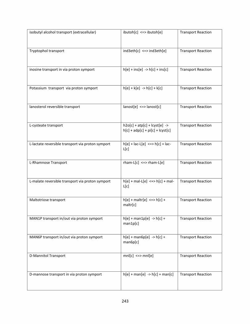
243

isobutyl alcohol transport (extracellular) ibutoh[c] <=> ibutoh[e] Transport Reaction

Tryptophol transport ind3eth[c] <=> ind3eth[e] Transport Reaction

inosine transport in via proton symport h[e] + ins[e] -> h[c] + ins[c] Transport Reaction

Potassium transport via proton symport h[e] + k[e] -> h[c] + k[c] Transport Reaction

lanosterol reversible transport lanost[e] <=> lanost[c] Transport Reaction

L-cysteate transport h2o[c] + atp[c] + lcyst[e] -> h[c] + adp[c] + pi[c] + lcyst[c]

Transport Reaction

L-lactate reversible transport via proton symport h[e] + lac-L[e] <=> h[c] + lac-L[c]

Transport Reaction

L-Rhamnose Transport rham-L[c] <=> rham-L[e] Transport Reaction

L-malate reversible transport via proton symport h[e] + mal-L[e] <=> h[c] + mal-L[c]

Transport Reaction

Maltotriose transport h[e] + maltr[e] <=> h[c] + maltr[c]

Transport Reaction

MAN1P transport in/out via proton symport h[e] + man1p[e] -> h[c] + man1p[c]

Transport Reaction

MAN6P transport in/out via proton symport h[e] + man6p[e] -> h[c] + man6p[c]

Transport Reaction

D-Mannitol Transport mnl[c] <=> mnl[e] Transport Reaction

D-mannose transport in via proton symport h[e] + man[e] -> h[c] + man[c] Transport Reaction

244

NADP transporter nadp[c] <=> nadp[e] Transport Reaction

nmntp h[e] + nmn[e] -> h[c] + nmn[c] Transport Reaction

o2 transport (diffusion) o2[e] <=> o2[c] Transport Reaction

Oxaloacetate transport oaa[c] <=> oaa[e] Transport Reaction

Octadecanoate (n-C18:0), Transport ocdca[e] <=> ocdca[c] Transport Reaction

Octadecenoate (n-C18:1), Transport ocdcea[e] <=> ocdcea[c] Transport Reaction

Octadecatrienoate, Transport ocdcta[e] <=> ocdcta[c] Transport Reaction

Octadecadienoate (n-C18:2), Transport ocdcya[e] <=> ocdcya[c] Transport Reaction

Octanoate (n-C8:0), Transport octa[e] <=> octa[c] Transport Reaction

5-oxoproline transport opro-L[c] <=> opro-L[e] Transport Reaction

Phenylacetaldehyde transport (extracellular) pacald[c] <=> pacald[e] Transport Reaction

PAP reversible uniport pap[e] <=> pap[c] Transport Reaction

Phosphoenolpyruvate transport in via proton symport

h[e] + pep[e] -> h[c] + pep[c] Transport Reaction

diphosphate transport in via ABC system h2o[c] + atp[c] + ppi[e] -> h[c] + adp[c] + pi[c] + ppi[c]

Transport Reaction

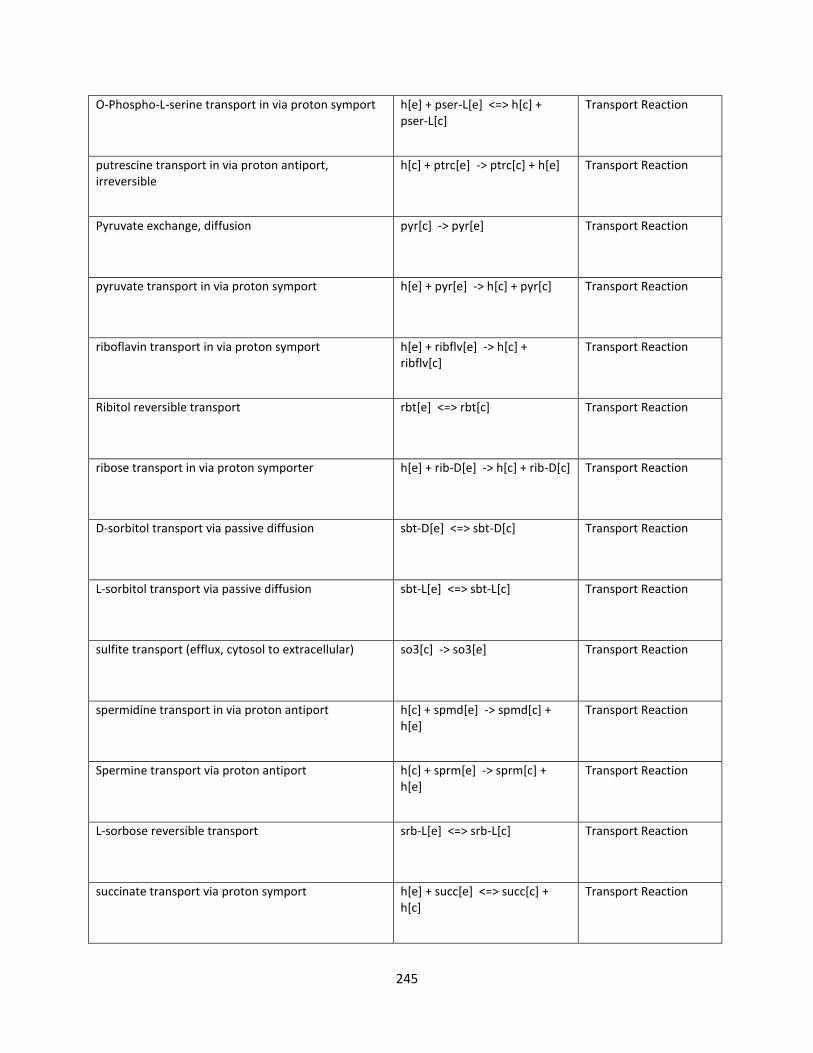
245

O-Phospho-L-serine transport in via proton symport h[e] + pser-L[e] <=> h[c] + pser-L[c]

Transport Reaction

putrescine transport in via proton antiport, irreversible

h[c] + ptrc[e] -> ptrc[c] + h[e] Transport Reaction

Pyruvate exchange, diffusion pyr[c] -> pyr[e] Transport Reaction

pyruvate transport in via proton symport h[e] + pyr[e] -> h[c] + pyr[c] Transport Reaction

riboflavin transport in via proton symport h[e] + ribflv[e] -> h[c] + ribflv[c]

Transport Reaction

Ribitol reversible transport rbt[e] <=> rbt[c] Transport Reaction

ribose transport in via proton symporter h[e] + rib-D[e] -> h[c] + rib-D[c] Transport Reaction

D-sorbitol transport via passive diffusion sbt-D[e] <=> sbt-D[c] Transport Reaction

L-sorbitol transport via passive diffusion sbt-L[e] <=> sbt-L[c] Transport Reaction

sulfite transport (efflux, cytosol to extracellular) so3[c] -> so3[e] Transport Reaction

spermidine transport in via proton antiport h[c] + spmd[e] -> spmd[c] + h[e]

Transport Reaction

Spermine transport via proton antiport h[c] + sprm[e] -> sprm[c] + h[e]

Transport Reaction

L-sorbose reversible transport srb-L[e] <=> srb-L[c] Transport Reaction

succinate transport via proton symport h[e] + succ[e] <=> succ[c] + h[c]

Transport Reaction

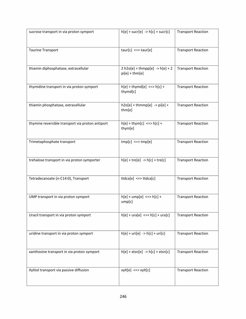
246

sucrose transport in via proton symport h[e] + sucr[e] -> h[c] + sucr[c] Transport Reaction

Taurine Transport taur[c] <=> taur[e] Transport Reaction

thiamin diphosphatase, extracellular 2 h2o[e] + thmpp[e] -> h[e] + 2 pi[e] + thm[e]

Transport Reaction

thymidine transport in via proton symport h[e] + thymd[e] <=> h[c] + thymd[c]

Transport Reaction

thiamin phosphatase, extracellular h2o[e] + thmmp[e] -> pi[e] + thm[e]

Transport Reaction

thymine reversible transport via proton antiport h[e] + thym[c] <=> h[c] + thym[e]

Transport Reaction

Trimetaphosphate transport tmp[c] <=> tmp[e] Transport Reaction

trehalose transport in via proton symporter h[e] + tre[e] -> h[c] + tre[c] Transport Reaction

Tetradecanoate (n-C14:0), Transport ttdca[e] <=> ttdca[c] Transport Reaction

UMP transport in via proton symport h[e] + ump[e] <=> h[c] + ump[c]

Transport Reaction

Uracil transport in via proton symport h[e] + ura[e] <=> h[c] + ura[c] Transport Reaction

uridine transport in via proton symport h[e] + uri[e] -> h[c] + uri[c] Transport Reaction

xanthosine transport in via proton symport h[e] + xtsn[e] -> h[c] + xtsn[c] Transport Reaction

Xylitol transport via passive diffusion xylt[e] <=> xylt[c] Transport Reaction

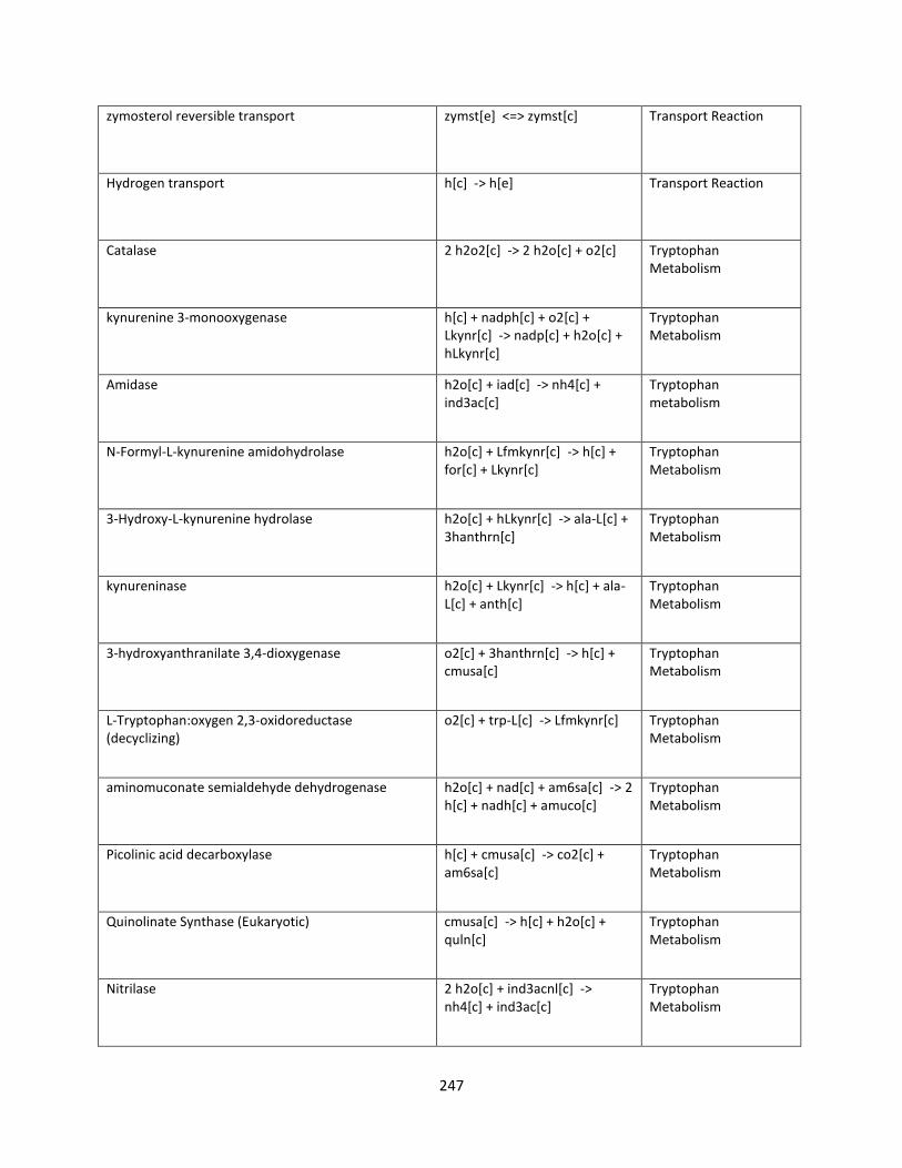
247

zymosterol reversible transport zymst[e] <=> zymst[c] Transport Reaction

Hydrogen transport h[c] -> h[e] Transport Reaction

Catalase 2 h2o2[c] -> 2 h2o[c] + o2[c] Tryptophan Metabolism

kynurenine 3-monooxygenase h[c] + nadph[c] + o2[c] + Lkynr[c] -> nadp[c] + h2o[c] + hLkynr[c]

Tryptophan Metabolism

Amidase h2o[c] + iad[c] -> nh4[c] + ind3ac[c]

Tryptophan metabolism

N-Formyl-L-kynurenine amidohydrolase h2o[c] + Lfmkynr[c] -> h[c] + for[c] + Lkynr[c]

Tryptophan Metabolism

3-Hydroxy-L-kynurenine hydrolase h2o[c] + hLkynr[c] -> ala-L[c] + 3hanthrn[c]

Tryptophan Metabolism

kynureninase h2o[c] + Lkynr[c] -> h[c] + ala-L[c] + anth[c]

Tryptophan Metabolism

3-hydroxyanthranilate 3,4-dioxygenase o2[c] + 3hanthrn[c] -> h[c] + cmusa[c]

Tryptophan Metabolism

L-Tryptophan:oxygen 2,3-oxidoreductase (decyclizing)

o2[c] + trp-L[c] -> Lfmkynr[c] Tryptophan Metabolism

aminomuconate semialdehyde dehydrogenase h2o[c] + nad[c] + am6sa[c] -> 2 h[c] + nadh[c] + amuco[c]

Tryptophan Metabolism

Picolinic acid decarboxylase h[c] + cmusa[c] -> co2[c] + am6sa[c]

Tryptophan Metabolism

Quinolinate Synthase (Eukaryotic) cmusa[c] -> h[c] + h2o[c] + quln[c]

Tryptophan Metabolism

Nitrilase 2 h2o[c] + ind3acnl[c] -> nh4[c] + ind3ac[c]

Tryptophan Metabolism

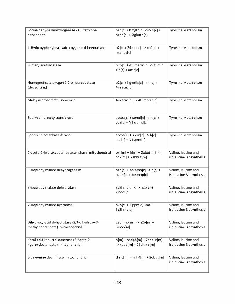
248

Formaldehyde dehydrogenase - Glutathione dependent

nad[c] + hmgth[c] <=> h[c] + nadh[c] + Sfglutth[c]

Tyrosine Metabolism

4-Hydroxyphenylpyruvate:oxygen oxidoreductase o2[c] + 34hpp[c] -> co2[c] + hgentis[c]

Tyrosine Metabolism

Fumarylacetoacetase h2o[c] + 4fumacac[c] -> fum[c] + h[c] + acac[c]

Tyrosine Metabolism

Homogentisate:oxygen 1,2-oxidoreductase (decyclizing)

o2[c] + hgentis[c] -> h[c] + 4mlacac[c]

Tyrosine Metabolism

Maleylacetoacetate isomerase 4mlacac[c] -> 4fumacac[c] Tyrosine Metabolism

Spermidine acetyltransferase accoa[c] + spmd[c] -> h[c] + coa[c] + N1aspmd[c]

Tyrosine Metabolism

Spermine acetyltransferase accoa[c] + sprm[c] -> h[c] + coa[c] + N1sprm[c]

Tyrosine Metabolism

2-aceto-2-hydroxybutanoate synthase, mitochondrial pyr[m] + h[m] + 2obut[m] -> co2[m] + 2ahbut[m]

Valine, leucine and isoleucine Biosynthesis

3-isopropylmalate dehydrogenase nad[c] + 3c2hmp[c] -> h[c] + nadh[c] + 3c4mop[c]

Valine, leucine and isoleucine Biosynthesis

3-isopropylmalate dehydratase 3c2hmp[c] <=> h2o[c] + 2ippm[c]

Valine, leucine and isoleucine Biosynthesis

2-isopropylmalate hydratase h2o[c] + 2ippm[c] <=> 3c3hmp[c]

Valine, leucine and isoleucine Biosynthesis

Dihydroxy-acid dehydratase (2,3-dihydroxy-3-methylpentanoate), mitochondrial

23dhmp[m] -> h2o[m] + 3mop[m]

Valine, leucine and isoleucine Biosynthesis

Ketol-acid reductoisomerase (2-Aceto-2-hydroxybutanoate), mitochondrial

h[m] + nadph[m] + 2ahbut[m] -> nadp[m] + 23dhmp[m]

Valine, leucine and isoleucine Biosynthesis

L-threonine deaminase, mitochondrial thr-L[m] -> nh4[m] + 2obut[m] Valine, leucine and isoleucine Biosynthesis

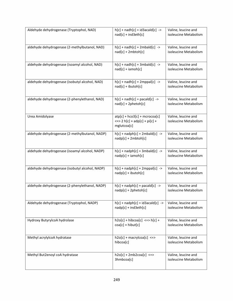
249

Aldehyde dehydrogenase (Tryptophol, NAD) h[c] + nadh[c] + id3acald[c] -> nad[c] + ind3eth[c]

Valine, leucine and isoleucine Metabolism

aldehyde dehydrogenase (2-methylbutanol, NAD) h[c] + nadh[c] + 2mbald[c] -> nad[c] + 2mbtoh[c]

Valine, leucine and isoleucine Metabolism

aldehyde dehydrogenase (isoamyl alcohol, NAD) h[c] + nadh[c] + 3mbald[c] -> nad[c] + iamoh[c]

Valine, leucine and isoleucine Metabolism

aldehyde dehydrogenase (isobutyl alcohol, NAD) h[c] + nadh[c] + 2mppal[c] -> nad[c] + ibutoh[c]

Valine, leucine and isoleucine Metabolism

aldehyde dehydrogenase (2-phenylethanol, NAD) h[c] + nadh[c] + pacald[c] -> nad[c] + 2phetoh[c]

Valine, leucine and isoleucine Metabolism

Urea Amidolyase atp[c] + hco3[c] + mcrocoa[c] <=> 2 h[c] + adp[c] + pi[c] + mglutcoa[c]

Valine, leucine and isoleucine Metabolism

aldehyde dehydrogenase (2-methylbutanol, NADP) h[c] + nadph[c] + 2mbald[c] -> nadp[c] + 2mbtoh[c]

Valine, leucine and isoleucine Metabolism

aldehyde dehydrogenase (isoamyl alcohol, NADP) h[c] + nadph[c] + 3mbald[c] -> nadp[c] + iamoh[c]

Valine, leucine and isoleucine Metabolism

aldehyde dehydrogenase (isobutyl alcohol, NADP) h[c] + nadph[c] + 2mppal[c] -> nadp[c] + ibutoh[c]

Valine, leucine and isoleucine Metabolism

aldehyde dehydrogenase (2-phenylethanol, NADP) h[c] + nadph[c] + pacald[c] -> nadp[c] + 2phetoh[c]

Valine, leucine and isoleucine Metabolism

Aldehyde dehydrogenase (Tryptophol, NADP) h[c] + nadph[c] + id3acald[c] -> nadp[c] + ind3eth[c]

Valine, leucine and isoleucine Metabolism

Hydroxy ButyrylcoA hydrolase h2o[c] + hibcoa[c] <=> h[c] + coa[c] + hibut[c]

Valine, leucine and isoleucine Metabolism

Methyl acrylylcoA hydratase h2o[c] + macrylcoa[c] <=> hibcoa[c]

Valine, leucine and isoleucine Metabolism

Methyl But2enoyl coA hydratase h2o[c] + 2mb2coa[c] <=> 3hmbcoa[c]

Valine, leucine and isoleucine Metabolism

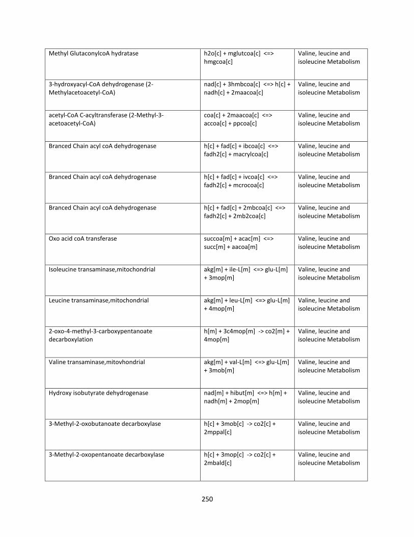
250

Methyl GlutaconylcoA hydratase h2o[c] + mglutcoa[c] <=> hmgcoa[c]

Valine, leucine and isoleucine Metabolism

3-hydroxyacyl-CoA dehydrogenase (2-Methylacetoacetyl-CoA)

nad[c] + 3hmbcoa[c] <=> h[c] + nadh[c] + 2maacoa[c]

Valine, leucine and isoleucine Metabolism

acetyl-CoA C-acyltransferase (2-Methyl-3-acetoacetyl-CoA)

coa[c] + 2maacoa[c] <=> accoa[c] + ppcoa[c]

Valine, leucine and isoleucine Metabolism

Branced Chain acyl coA dehydrogenase h[c] + fad[c] + ibcoa[c] <=> fadh2[c] + macrylcoa[c]

Valine, leucine and isoleucine Metabolism

Branced Chain acyl coA dehydrogenase h[c] + fad[c] + ivcoa[c] <=> fadh2[c] + mcrocoa[c]

Valine, leucine and isoleucine Metabolism

Branced Chain acyl coA dehydrogenase h[c] + fad[c] + 2mbcoa[c] <=> fadh2[c] + 2mb2coa[c]

Valine, leucine and isoleucine Metabolism

Oxo acid coA transferase succoa[m] + acac[m] <=> succ[m] + aacoa[m]

Valine, leucine and isoleucine Metabolism

Isoleucine transaminase,mitochondrial akg[m] + ile-L[m] <=> glu-L[m] + 3mop[m]

Valine, leucine and isoleucine Metabolism

Leucine transaminase,mitochondrial akg[m] + leu-L[m] <=> glu-L[m] + 4mop[m]

Valine, leucine and isoleucine Metabolism

2-oxo-4-methyl-3-carboxypentanoate decarboxylation

h[m] + 3c4mop[m] -> co2[m] + 4mop[m]

Valine, leucine and isoleucine Metabolism

Valine transaminase,mitovhondrial akg[m] + val-L[m] <=> glu-L[m] + 3mob[m]

Valine, leucine and isoleucine Metabolism

Hydroxy isobutyrate dehydrogenase nad[m] + hibut[m] <=> h[m] + nadh[m] + 2mop[m]

Valine, leucine and isoleucine Metabolism

3-Methyl-2-oxobutanoate decarboxylase h[c] + 3mob[c] -> co2[c] + 2mppal[c]

Valine, leucine and isoleucine Metabolism

3-Methyl-2-oxopentanoate decarboxylase h[c] + 3mop[c] -> co2[c] + 2mbald[c]

Valine, leucine and isoleucine Metabolism

251

4-Methyl-2-oxopentanoate decarboxylase h[c] + 4mop[c] -> co2[c] + 3mbald[c]

Valine, leucine and isoleucine Metabolism

2-oxoisovalerate dehydrogenase nad[c] + coa[c] + 3mop[c] <=> nadh[c] + co2[c] + 2mbcoa[c]

Valine, leucine and isoleucine Metabolism

Keto-Isocaproate dehydrogenase coa[m] + nad[m] + 4mop[m] <=> h[m] + nadh[m] + ivcoa[m]

Valine, leucine and isoleucine Metabolism

2-Oxovalerate dehydrogenase coa[m] + nad[m] + 3mob[m] <=> h[m] + nadh[m] + ibcoa[m]

Valine, leucine and isoleucine Metabolism

Isoleucine transaminase akg[c] + ile-L[c] <=> glu-L[c] + 3mop[c]

Valine, leucine and isoleucine Metabolism

Leucine transaminase akg[c] + leu-L[c] <=> glu-L[c] + 4mop[c]

Valine, leucine and isoleucine Metabolism

2-Oxo-4-methyl-3-carboxypentanoate decarboxylation

h[c] + 3c4mop[c] -> co2[c] + 4mop[c]

Valine, leucine and isoleucine Metabolism

Valine transaminase val-L[c] + akg[c] <=> 3mob[c] + glu-L[c]

Valine, leucine and isoleucine Metabolism

Pyridoxamine kinase atp[c] + pydam[c] -> h[c] + adp[c] + pyam5p[c]

Vitamin B6 Metabolism

Pyridoxal kinase atp[c] + pydx[c] -> h[c] + adp[c] + pydx5p[c]

Vitamin B6 Metabolism

Pyridoxine kinase atp[c] + pydxn[c] -> h[c] + adp[c] + pdx5p[c]

Vitamin B6 Metabolism

Pyridoxine 5'-phosphate oxidase o2[c] + pdx5p[c] <=> h2o2[c] + pydx5p[c]

Vitamin B6 Metabolism

Pyridoxamine 5'-phosphate oxidase h2o[c] + o2[c] + pyam5p[c] -> nh4[c] + h2o2[c] + pydx5p[c]

Vitamin B6 Metabolism

Pyridoxine oxidase o2[c] + pydxn[c] -> h2o2[c] + pydx[c]

Vitamin B6 Metabolism

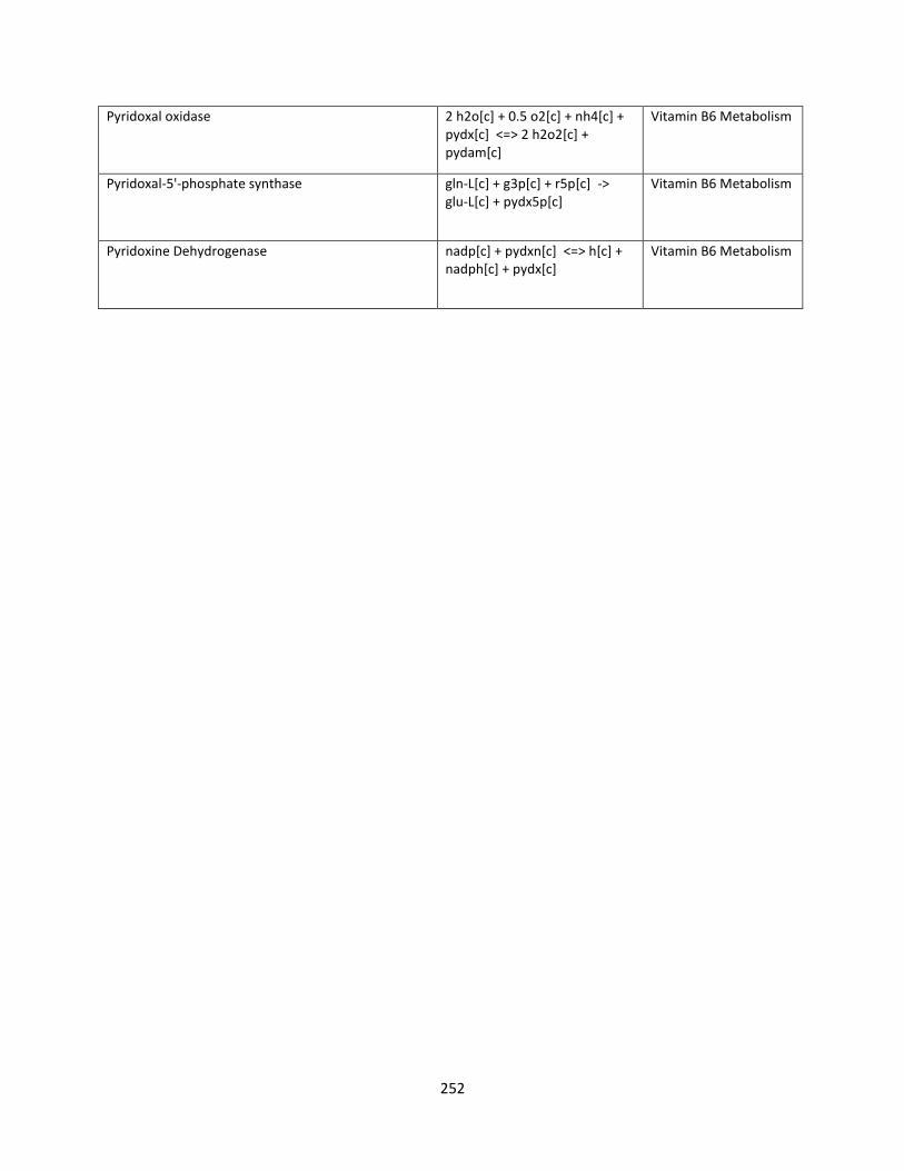
252

Pyridoxal oxidase 2 h2o[c] + 0.5 o2[c] + nh4[c] + pydx[c] <=> 2 h2o2[c] + pydam[c]

Vitamin B6 Metabolism

Pyridoxal-5'-phosphate synthase gln-L[c] + g3p[c] + r5p[c] -> glu-L[c] + pydx5p[c]

Vitamin B6 Metabolism

Pyridoxine Dehydrogenase nadp[c] + pydxn[c] <=> h[c] + nadph[c] + pydx[c]

Vitamin B6 Metabolism

253

A5 Metabolite list in iAD828

Abbreviations Full name

10ft 10-Formyltetrahydrofolate

12dgr 1,2-Diacylglycerol

13BDglcn 1,3-beta-D-Glucan

13dpg 3-Phospho-D-glyceroyl phosphate

14glun (1,4-alpha-D-Glucosyl)n

1ag3p 1-Acyl-sn-glycerol 3-phosphate

1agly3p 1-Acyl-glycerone 3-phosphate

1agpc acyl-glycerophosphocholine

1pyr5c 1-Pyrroline-5-carboxylate

23dhdp 2,3-Dihydrodipicolinate

23dhmb (R)-2,3-Dihydroxy-3-methylbutanoate

23dph 2,3-Bisphospho-D-glycerate

23drhamn 2-Dehydro-3-deoxy-L-rhamnonate

25aics (S)-2-[5-Amino-1-(5-phospho-D-ribosyl)imidazole-4-carboxamido]succinate

25dhpp 2,5-Diamino-6-hydroxy-4-(5-phosphoribosylamino)-pyrimidine

2ahbut (S)-2-Aceto-2-hydroxybutanoate

2ahhmd 2-Amino-4-hydroxy-6-hydroxymethyl-7,8-dihydropteridine diphosphate

2ahhmp 2-Amino-4-hydroxy-6-hydroxymethyl-7,8-dihydropteridine

2cpr5p 1-(2-Carboxyphenylamino)-1-deoxy-D-ribulose 5-phosphate

2dda7p 2-Dehydro-3-deoxy-D-arabino-heptonate 7-phosphate

2dhp 2-Dehydropantoate

2dr1p 2-Deoxy-D-ribose 1-phosphate

2dr5p 2-Deoxy-D-ribose 5-phosphate

2glcna 2-Dehydro-D-gluconate

2hhxdal 2-Hydroxy-hexadecanal

2hp6mbq 2-Hexaprenyl-6-methoxy-1,4-benzoquinone

2hp6mp 2-Hexaprenyl-6-methoxyphenol

2hpmhmbq 2-Hexaprenyl-3-methyl-5-hydroxy-6-methoxy-1,4-benzoquinone

2hpmmbq 2-Hexaprenyl-3-methyl-6-methoxy-1,4-benzoquinone

2ins 2-Inosose

2ippm 2-Isopropylmaleate

2kmb 2-keto-4-methylthiobutyrate

254

2maacoa 2-Methyl-3-acetoacetyl-CoA

2mahmp 2-Methyl-4-amino-5-hydroxymethylpyrimidine diphosphate

2mb2coa trans-2-Methylbut-2-enoyl-CoA

2mbald 2-Methylbutanal

2mbcoa 2-Methylbutanoyl-CoA

2mbtoh 2-Methyl Butanol

2mcit 2-Methylcitrate

2mop 2-Methyl-3-oxopropanoate

2mppal 2-Methyl 1- Propanal

2obut 2-Oxobutanoate

2oxoadp 2-Oxoadipate

2pg D-Glycerate 2-phosphate

2pglyc 2-Phosphoglycolate

2phetoh 2-Phenylethanol

34hpp 3-(4-Hydroxyphenyl)pyruvate

3c2hmp 3-Carboxy-2-hydroxy-4-methylpentanoate

3c3hmp 3-Carboxy-3-hydroxy-4-methylpentanoate

3c4mop 3-Carboxy-4-methyl-2-oxopentanoate

3dh5hpb 3-Hexaprenyl-4,5-dihydroxybenzoate

3dhq 3-Dehydroquinate

3dhsk 3-Dehydroshikimate

3dsphgn 3-Dehydrosphinganine

3hanthrn 3-Hydroxyanthranilate

3hmbcoa (S)-3-Hydroxy-2-methylbutyryl-CoA

3hph5mb 3-Hexaprenyl-4-hydroxy-5-methoxybenzoate

3ig3p C-(3-Indolyl)-glycerol 3-phosphate

3mbald 3-Methylbutanal

3mob 3-Methyl-2-oxobutanoate

3mop (S)-3-Methyl-2-oxopentanoate

3ophb_5 3-Hexaprenyl-4-hydroxybenzoate

3pg 3-Phospho-D-glycerate

3php 3-Phosphohydroxypyruvate

3psme 5-O-(1-Carboxyvinyl)-3-phosphoshikimate

44mctr 4,4-dimethylcholesta-8,14,24-trienol

44mzym 4,4-dimethyllanosterol

4abut 4-Aminobutanoate

4abz 4-Aminobenzoate

4adcho 4-amino-4-deoxychorismate

255

4ahmmp 4-Amino-5-hydroxymethyl-2-methylpyrimidine

4ampm 4-Amino-2-methyl-5-phosphomethylpyrimidine

4fumacac 4-Fumarylacetoacetate

4h2oglt 4-Hydroxy-2-oxoglutarate

4hbz 4-Hydroxybenzoate

4hpro-LT trans-4-Hydroxy-L-proline

4mhetz 4-Methyl-5-(2-hydroxyethyl)-thiazole

4mlacac 4-Maleylacetoacetate

4mop 4-Methyl-2-oxopentanoate

4mpetz 4-Methyl-5-(2-phosphoethyl)-thiazole

4mzym 4-methylzymosterol

4mzym_int1 4alpha-Methylzymosterol-4-carboxylate

4mzym_int2 3-Keto-4-methylzymosterol

4pasp 4-Phospho-L-aspartate

4ppan D-4-Phosphopantothenate

4ppcys N-((R)-4-Phosphopantothenoyl)-L-cysteine

4r5au 4-(1-D-Ribitylamino)-5-aminouracil

5aizc 5-amino-1-(5-phospho-D-ribosyl)imidazole-4-carboxylate

5aop 5-Amino-4-oxopentanoate

5aprbu 5-Amino-6-(5-phosphoribitylamino)uracil

5apru 5-Amino-6-(5-phosphoribosylamino)uracil

5dpmev (R)-5-Diphosphomevalonate

5fthf 5-Formyltetrahydrofolate

5mdr1p 5-Methylthio-5-deoxy-D-ribose 1-phosphate

5mdru1p 5-Methylthio-5-deoxy-D-ribulose 1-phosphate

5mta 5-Methylthioadenosine

5mthf 5-Methyltetrahydrofolate

5pmev (R)-5-Phosphomevalonate

6pgc 6-Phospho-D-gluconate

6pgc 6-Phospho-D-gluconate

6pgl 6-phospho-D-glucono-1,5-lactone

8aonn 8-Amino-7-oxononanoate

aacoa Acetoacetyl-CoA

abt-D D- Arabitol

abt-L L-Arabitol

ac Acetate

acac Acetoacetate

acACP Acetyl-ACP

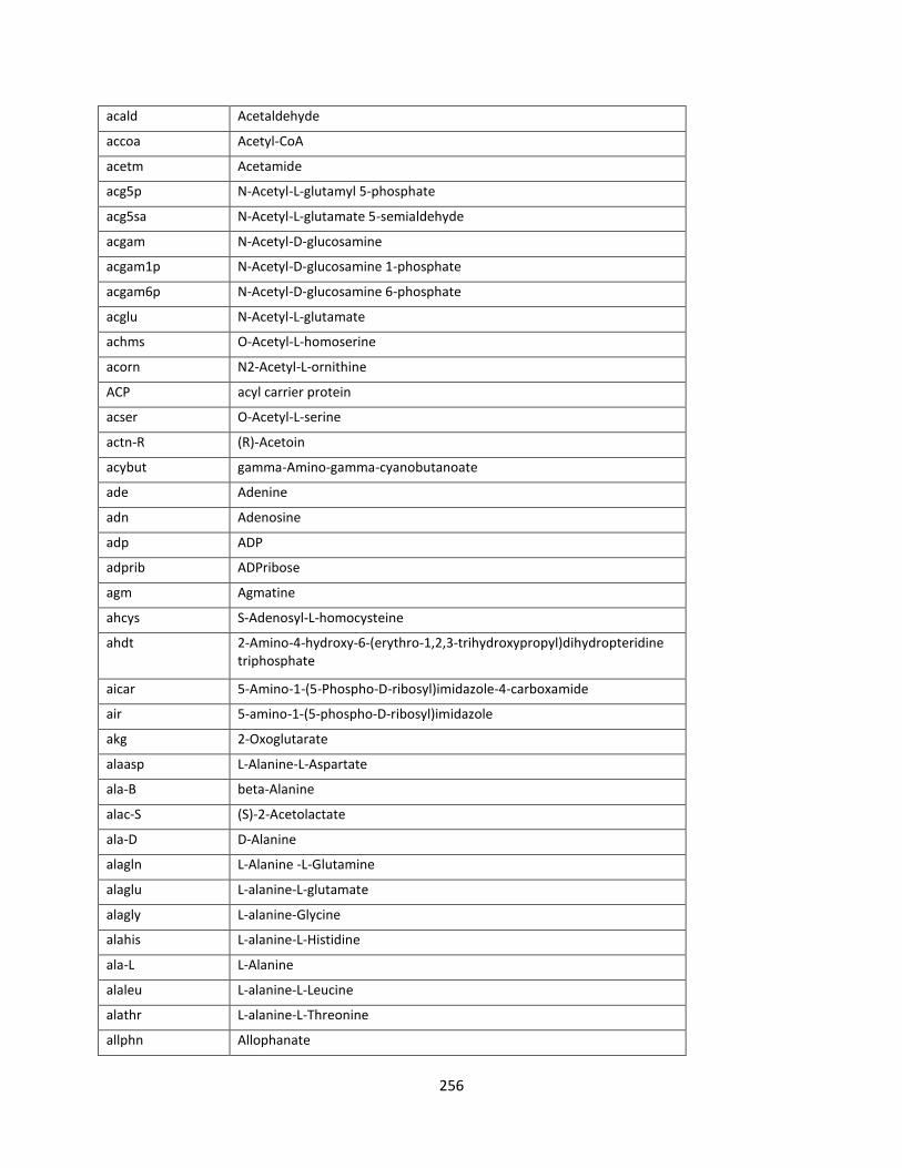
256

acald Acetaldehyde

accoa Acetyl-CoA

acetm Acetamide

acg5p N-Acetyl-L-glutamyl 5-phosphate

acg5sa N-Acetyl-L-glutamate 5-semialdehyde

acgam N-Acetyl-D-glucosamine

acgam1p N-Acetyl-D-glucosamine 1-phosphate

acgam6p N-Acetyl-D-glucosamine 6-phosphate

acglu N-Acetyl-L-glutamate

achms O-Acetyl-L-homoserine

acorn N2-Acetyl-L-ornithine

ACP acyl carrier protein

acser O-Acetyl-L-serine

actn-R (R)-Acetoin

acybut gamma-Amino-gamma-cyanobutanoate

ade Adenine

adn Adenosine

adp ADP

adprib ADPribose

agm Agmatine

ahcys S-Adenosyl-L-homocysteine

ahdt 2-Amino-4-hydroxy-6-(erythro-1,2,3-trihydroxypropyl)dihydropteridine triphosphate

aicar 5-Amino-1-(5-Phospho-D-ribosyl)imidazole-4-carboxamide

air 5-amino-1-(5-phospho-D-ribosyl)imidazole

akg 2-Oxoglutarate

alaasp L-Alanine-L-Aspartate

ala-B beta-Alanine

alac-S (S)-2-Acetolactate

ala-D D-Alanine

alagln L-Alanine -L-Glutamine

alaglu L-alanine-L-glutamate

alagly L-alanine-Glycine

alahis L-alanine-L-Histidine

ala-L L-Alanine

alaleu L-alanine-L-Leucine

alathr L-alanine-L-Threonine

allphn Allophanate

257

alltn Allantoin

alltt Allantoate

alpam S-aminomethyldihydrolipoamide

am6sa 2-Aminomuconate 6-semialdehyde

amacald Aminoacetaldehyde

amet S-Adenosyl-L-methionine

ametam S-Adenosylmethioninamine

amob S-Adenosyl-4-methylthio-2-oxobutanoate

amp AMP

amuco 2-Aminomuconate

anth Anthranilate

ap4g P1-(5-adenosyl),P4-(5-guanosyl) tetraphosphate

aproa 3-Aminopropanal

aprop alpha-Aminopropiononitrile

aprut N-Acetylputrescine

aps Adenosine 5-phosphosulfate

arab-D D-Arabinose

arab-L L-Arabinose

arg-L L-Arginine

argsuc N(omega)-(L-Arginino)succinate

asn-L L-Asparagine

asp-L L-Aspartate

aspsa L-Aspartate 4-semialdehyde

atp ATP

b124tc But-1-ene-1,2,4-tricarboxylate

bf26p beta-D-Fructose 2,6-phosphate

bf6p beta-D-Fructose 6-bisphosphate

btd-RR (R,R)-2,3-Butanediol

btn Biotin

camp cAMP

cbasp N-Carbamoyl-L-aspartate

cbp Carbamoyl phosphate

cdp CDP

cdpchol CDPcholine

cdpdag CDPdiacylglycerol

cdpea CDPethanolamine

cellb Cellobiose

cer1_24 Ceramide-1 (Sphinganine:n-C24:0)

258

cer1_26 Ceramide-1 (Sphinganine:n-C26:0)

cer2_24 Ceramide-2 (Phytosphingosine:n-C24:0)

cer2_26 Ceramide-2 (Phytosphingosine:n-C26:0)

cer3 N-Acylsphingosine

cer3_24 Ceramide-3 (Phytosphingosine:n-C24:0OH)

cer3_26 Ceramide-3 (Phytosphingosine:n-C26:0OH)

cgly Cys-Gly

ch4s Methanethiol

chitin Chitin (monomer)

chitos Chitosan

chol Choline

chor chorismate

cit Citrate

citr-L L-Citrulline

citr-L L-Citrulline

clpn Cardiolipin

cmp CMP

cmusa 2-Amino-3-carboxymuconate semialdehyde

co2 Carbon dioxide

coa Coenzyme A

cpppg3 Coproporphyrinogen III

csn Cytosine

ctp CTP

cys-L L-Cysteine

cyst-L L-Cystathionine

cytd Cytidine

dad-2 Deoxyadenosine

dadp dADP

damp dAMP

dann 7,8-Diaminononanoate

datp dATP

db4p 3,4-dihydroxy-2-butanone 4-phosphate

dca Decanoate (n-C10:0)

dcaACP Decanoyl-ACP (n-C10:0ACP)

dcacoa Decanoyl-CoA (n-C10:0CoA)

dcamp N6-(1,2-Dicarboxyethyl)-AMP

dcdp dCDP

dcmp dCMP

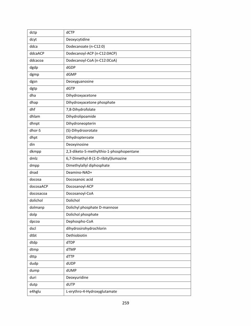
259

dctp dCTP

dcyt Deoxycytidine

ddca Dodecanoate (n-C12:0)

ddcaACP Dodecanoyl-ACP (n-C12:0ACP)

ddcacoa Dodecanoyl-CoA (n-C12:0CoA)

dgdp dGDP

dgmp dGMP

dgsn Deoxyguanosine

dgtp dGTP

dha Dihydroxyacetone

dhap Dihydroxyacetone phosphate

dhf 7,8-Dihydrofolate

dhlam Dihydrolipoamide

dhnpt Dihydroneopterin

dhor-S (S)-Dihydroorotate

dhpt Dihydropteroate

din Deoxyinosine

dkmpp 2,3-diketo-5-methylthio-1-phosphopentane

dmlz 6,7-Dimethyl-8-(1-D-ribityl)lumazine

dmpp Dimethylallyl diphosphate

dnad Deamino-NAD+

docosa Docosanoic acid

docosaACP Docosanoyl-ACP

docosacoa Docosanoyl-CoA

dolichol Dolichol

dolmanp Dolichyl phosphate D-mannose

dolp Dolichol phosphate

dpcoa Dephospho-CoA

dscl dihydrosirohydrochlorin

dtbt Dethiobiotin

dtdp dTDP

dtmp dTMP

dttp dTTP

dudp dUDP

dump dUMP

duri Deoxyuridine

dutp dUTP

e4hglu L-erythro-4-Hydroxyglutamate

260

e4p D-Erythrose 4-phosphate

eicosa Eicosanoic acid

eicosaACP Eicosanoyl - ACP

eicosacoa Eicosanoyl-CoA

eicosapen Eicosapentaenoic acid

eicosapenACP Eicosapentanoyl - ACP

eicosapencoa Icosapentaenoyl-CoA

eig3p D-erythro-1-(Imidazol-4-yl)glycerol 3-phosphate

epist episterol

ergst Ergosterol

ergtetrol Ergosta-5,7,22,24,(28)-tetraen-3beta-ol

ergtrol ergosta-5,7,24(28)-trienol

etha Ethanolamine

ethamp Ethanolamine phosphate

etoh Ethanol

f6p D-Fructose 6-phosphate

fad Flavin adenine dinucleotide oxidized

fadh2 Flavin adenine dinucleotide reduced

fdp D-Fructose 1,6-bisphosphate

fe2 Fe2+

fecost fecosterol

fgam N2-Formyl-N1-(5-phospho-D-ribosyl)glycinamide

ficytb5 Ferricytochrome b5

ficytc Ferricytochrome c

fmn FMN

focytb5 Ferrocytochrome b5

focytc Ferrocytochrome c

for Formate

fpram 2-(Formamido)-N1-(5-phospho-D-ribosyl)acetamidine

fprica 5-Formamido-1-(5-phospho-D-ribosyl)imidazole-4-carboxamide

frdp Farnesyl diphosphate

frmd Formamide

fru D-Fructose

fuc1p L-Fuculose 1-phosphate

fum Fumarate

g15lac D-Glucono-1,5-lactone

g1p D-Glucose 1-phosphate

261

g3p Glyceraldehyde 3-phosphate

g3pc sn-Glycero-3-phosphocholine

g3pi sn-Glycero-3-phospho-1-inositol

g6p D-Glucose 6-phosphate

gal D-Galactose

gal14lac D-Galactono-1,4-lactone

gal1p alpha-D-Galactose 1-phosphate

gam6p D-Glucosamine 6-phosphate

gar N1-(5-Phospho-D-ribosyl)glycinamide

gcald Glycolaldehyde

gcylcer Glucosylceramide

gdp GDP

gdpmann GDP-D-mannose

ggdp Geranylgeranyl diphosphate

glc-D D-Glucose

glcn-D D-Gluconic acid

gln-L L-Glutamine

glu5p L-Glutamate 5-phosphate

glu5sa L-Glutamate 5-semialdehyde

gluala 5-L-Glutamyl-L-alanine

glucoa Glutaryl-CoA

glucys gamma-L-Glutamyl-L-cysteine

glu-L L-Glutamate

glx Glyoxylate

gly Glycine

glyasn Glycyl Asparagine

glyasp Glycyl Aspartate

glyc Glycerol

glyc3p Glycerol 3-phosphate

glyclt Glycolate

glycogen glycogen

glygln Glycyl Glutamine

glyglu Glycyl Glutamate

glymet Glycyl Methionine

glypro Glycyl Proline

gmp GMP

gp4g P1,P4-Bis(5-guanosyl) tetraphosphate

grdp Geranyl diphosphate

262

gsn Guanosine

gthox Oxidized glutathione

gthrd Reduced glutathione

gtp GTP

gua Guanine

h H+

h2o H2O

h2o2 Hydrogen peroxide

h2s Hydrogen sulfide

hco3 Bicarbonate

hcys-L L-Homocysteine

hdca Hexadecanoate (n-C16:0)

hdcea Hexadecenoate (n-C16:1)

hdceaACP Hexadecenoyl ACP

hdceacoa Hexadecenoyl coA

hemeA Heme A

hemeO Heme O

hepdca Heptadecanoate

hepdcaACP Heptadecanoyl-ACP

hepdcacoa Heptadecanoyl-CoA

hepdcea Heptadecenoate

hepdceaACP Heptadecenoyl-ACP

hepdceacoa Heptadecenoyl-CoA

hexa Hexanoate

hexaACP Hexanoyl-ACP

hexacoa Hexanoyl-CoA

hexc hexacosanoate (n-C26:0)

hexcACP Hexacosanoyl-ACP

hexccoa Hexacosanoyl-CoA (n-C26:0CoA)

hexdp all-trans-Hexaprenyl diphosphate

hgentis Homogentisate

hibcoa (S)-3-Hydroxyisobutyryl-CoA

hibut (S)-3-Hydroxyisobutyrate

hicit Homoisocitrate

his-L L-Histidine

hisp L-Histidinol phosphate

histd L-Histidinol

hLkynr 3-Hydroxy-L-kynurenine

263

hmbil Hydroxymethylbilane

hmgcoa Hydroxymethylglutaryl-CoA

hmgth hydroxymethylglutathione

hom-L L-Homoserine

hpglu Tetrahydropteroyltri-L-glutamate

hppcoa 3-Hydroxypropionyl-CoA

hxan Hypoxanthine

hxdcal Hexadecanal

iad Indole-3-acetamide

iamoh 3-Methylbutanol

iamoh 3-Methylbutanol

iasp Iminoaspartate

ibcoa Isobutyryl-CoA

ibutoh Isobutyl alcohol

icit Isocitrate

id3acald Indole-3-acetaldehyde

idp IDP

ile-L L-Isoleucine

imacp 3-(Imidazol-4-yl)-2-oxopropyl phosphate

imp IMP

ind3ac Indole-3-acetate

ind3acnl Indole-3-acetonitrile

ind3eth Indole-3-ethanol

indpyr Indolepyruvate

inost myo-Inositol

ins Inosine

ipc124 Inositol phosphorylceramide, ceramide-1 (24C) (IPC24C)

ipc126 Inositol phosphorylceramide, ceramide-1 (26C)

ipc224 Inositol-phosphorylceramide-ceramide-2-24C

ipc226 Inositol phosphorylceramide, ceramide-2 (26C)

ipdp Isopentenyl diphosphate

itp ITP

ivcoa Isovaleryl-CoA

k potassium

L2aadp L-2-Aminoadipate

L2aadp6sa L-2-Aminoadipate 6-semialdehyde

lac-D D-Lactate

lac-L L-Lactate

264

lact Lactose

lact Lactose

lactcer Lactosylceramide

lald-S (S)-Lactaldehyde

lanost Lanosterol

lcyst L-Cysteate

leu-L L-Leucine

Lfmkynr L-Formylkynurenine

lgt-S (R)-S-Lactoylglutathione

Lkynr L-Kynurenine

lpam Lipoamide

lys-L L-Lysine

macrylcoa Methacrylyl-CoA

madg alpha-Methyl-D-glucoside

malACP Malonyl-[acyl-carrier protein]

malcoa Malonyl-CoA

mal-L L-Malate

malt Maltose

maltr Maltotriose

man D-Mannose

man1p D-Mannose 1-phosphate

man1p D-Mannose 1-phosphate

man2mi1p-D D-Mannose Inositol Phosphate 2

man6p D-Mannose 6-phosphate

manmi1p-D D-Mannose Inositol Phosphate

mannan Mannan

mbdg beta-Methylglucoside

mcrocoa 3-Methylcrotonyl-CoA

meoh Methanol

metala Methionine-Alanine

methf 5,10-Methenyltetrahydrofolate

methf 5,10-Methenyltetrahydrofolate

met-L L-Methionine

met-L L-Methionine

mev-R (R)-Mevalonate

mglutcoa 3-Methylglutaconyl-CoA

mhpglu 5-Methyltetrahydropteroyltri-L-glutamate

mi145tp-D D-myo-Inositol 1,4,5-trisphosphate

265

mi14bp-D D-myo-Inositol 1,4-bisphosphate

mi1p-D 1D-myo-Inositol 1-phosphate

micit methylisocitrate

mip2c124 mannose-(inositol-P)2-ceramide, ceramide-1 (24C)

mip2c126 mannose-(inositol-P)2-ceramide, ceramide-1 (26C)

mip2c224 mannose-(inositol-P)2-ceramide, ceramide-2 (24C)

mip2c226 mannose-(inositol-P)2-ceramide, ceramide-2 (26C)

mipc124 mannose-inositol phosphorylceramide, ceramide-1 (24C)

mipc126 mannose-inositol phosphorylceramide, ceramide-1 (26C)

mipc224 mannose-inositol phosphorylceramide, ceramide-2 (24C)

mipc226 mannose-inositol phosphorylceramide, ceramide-2 (26C)

mlthf 5,10-Methylenetetrahydrofolate

mnl D-Mannitol

msa Malonate semialdehyde

mthgxl Methylglyoxal

myrsACP Myristoyl-ACP (n-C14:0ACP)

N1aspmd N1-Acetylspermidine

N1sprm N1-Acetylspermine

Na Sodium

nac Nicotinate

nad Nicotinamide adenine dinucleotide

nadh Nicotinamide adenine dinucleotide - reduced

nadp Nicotinamide adenine dinucleotide phosphate

nadph Nicotinamide adenine dinucleotide phosphate - reduced

ncam Nicotinamide

nh4 Ammonium

nicrnt Nicotinate D-ribonucleotide

nmn NMN

o2 O2

oaa Oxaloacetate

ocdca octadecanoate (n-C18:0)

ocdcaACP Octadecanoyl-ACP (n-C18:0ACP)

ocdcea octadecenoate (n-C18:1)

ocdceaACP octadecenoyl-ACP

ocdceacoa octadecenoyl-coA

ocdcta Octadecatrienoate

ocdctaACP Octadecatrienoyl-ACP

ocdctacoa Octadecatrienoyl-CoA

266

ocdcya octadecadienoate (n-C18:2)

ocdcyaACP Octadecynoyl-ACP (n-C18:2ACP)

ocdcyacoa Octadecynoyl-CoA-n-C182CoA

octa octanoate (n-C8:0)

octaACP Octanoyl-ACP

octacoa Octanoyl-CoA

opro-L 5-Oxoproline

orn Ornithine

orot Orotate

orot5p Orotidine 5-phosphate

oxag Oxaloglutarate

pa Phosphatidate

pac Phenylacetic acid

pacald Phenylacetaldehyde

pad 2-Phenylacetamide

palmACP Palmitoyl-ACP (n-C16:0ACP)

pan4p Pantetheine 4-phosphate

pant-R (R)-Pantoate

pap Adenosine 3,5-bisphosphate

paps 3-Phosphoadenylyl sulfate

pc Phosphatidylcholine

pdx5p Pyridoxine 5-phosphate

pe phosphatidylethanolamine

pendp all-trans-Pentaprenyl diphosphate

pep Phosphoenolpyruvate

pg Phosphatidylglycerol

pgp Phosphatidylglycerophosphate

phe-L L-Phenylalanine

pheme Protoheme

phom O-Phospho-L-homoserine

phpyr Phenylpyruvate

pi Phosphate

pmtcoa Palmitoyl-CoA (n-C16:0CoA)

pnto-R (R)-Pantothenate

ppACP Propanoyl-ACP

ppbng Porphobilinogen

ppcoa Propanoyl-CoA

ppecoa Propenoyl-CoA

267

pphn Prephenate

ppi Diphosphate

ppp9 Protoporphyrin

pppg9 Protoporphyrinogen IX

pppi Inorganic triphosphate

pram 5-Phospho-beta-D-ribosylamine

pran N-(5-Phospho-D-ribosyl)anthranilate

prbamp 1-(5-Phosphoribosyl)-AMP

prbatp 1-(5-Phosphoribosyl)-ATP

prfp 1-(5-Phosphoribosyl)-5-[(5-phosphoribosylamino)methylideneamino]imidazole-4-carboxamide

prlp 5-[(5-phospho-1-deoxyribulos-1-ylamino)methylideneamino]-1-(5-phosphoribosyl)imidazole-4-carboxamide

pro-L L-Proline

prpp 5-Phospho-alpha-D-ribose 1-diphosphate

ps phosphatidylserine

pser-L O-Phospho-L-serine

psph1p Phytosphingosine 1-phosphate

psphings Phytosphingosine

ptd134bp phosphatidyl-1D-myo-inositol 3,4-bisphosphate

ptd145bp 1-Phosphatidyl-D-myo-inositol 4,5-bisphosphate

ptd1ino phosphatidyl-1D-myo-inositol

ptd2meeta Phosphatidyl-N-dimethylethanolamine

ptd3ino 1-Phosphatidyl-1D-myo-inositol 3-phosphate

ptd4ino 1-Phosphatidyl-1D-myo-inositol 4-phosphate

ptdmeeta Phosphatidyl-N-methylethanolamine

ptrc Putrescine

pyam5p Pyridoxamine 5-phosphate

pydam Pyridoxamine

pydx Pyridoxal

pydx5p Pyridoxal 5-phosphate

pydxn Pyridoxine

pyr Pyruvate

q6 Ubiquinone-6

q6h2 Ubiquinol-6

quln Quinolinate

r1p alpha-D-Ribose 1-phosphate

268

r5p alpha-D-Ribose 5-phosphate

rbl-D D-Ribulose

rbt Ribitol

rham-L L-Rhamnose

rhamlac L-Rhamnono-1,4-lactone

rhamn L-Rhamnonate

rib-D D-Ribose

ribflv Riboflavin

ribu-D D-Ribulose

rnam N-Ribosylnicotinamide

ru5p-D D-Ribulose 5-phosphate

s Sulfur

s7p Sedoheptulose 7-phosphate

saccrp-L L-Saccharopine

sbt-D D-Sorbitol

sbt-L L-Sorbitol

scl sirohydrochlorin

ser-L L-Serine

Sfglutth S-Formylglutathione

sheme Siroheme

skm Shikimate

skm5p Shikimate 5-phosphate

so3 Sulfite

so4 Sulfate

sph1p Sphinganine 1-phosphate

sphgn Sphinganine

spmd Spermidine

spmylin Sphingomyelin

sprm Spermine

sql Squalene

srb-L L-Sorbose

Ssq23epx (S)-Squalene-2,3-epoxide

stcoa Stearoyl-CoA (n-C18:0CoA)

succ Succinate

succoa Succinyl-CoA

succsal succsal[m]

suchms O-Succinyl-L-homoserine

sucr Sucrose

269

taur Taurine

tdcoa Tetradecanoyl-CoA (n-C14:0CoA)

thf 5,6,7,8-Tetrahydrofolate

thfglu Tetrahydrofolyl-[Glu](2)

thm Thiamin

thmpp Thiamine diphosphate

thmtp Thiamin triphosphate

thr-L L-Threonine

thym Thymine

thymd Thymidine

tmp Trimetaphosphate

trdox Oxidized thioredoxin

trdrd Reduced thioredoxin

tre Trehalose

tre6p alpha,alpha-Trehalose 6-phosphate

triglyc triglyceride

trp-L L-Tryptophan

ttc tetracosanoate (n-C24:0)

ttcACP tetracosanoyl-ACP

ttccoa tetracosanoyl-CoA (n-C24:0CoA)

ttdca tetradecanoate (n-C14:0)

tyr-L L-Tyrosine

uacgam UDP-N-acetyl-D-glucosamine

udp UDP

udpg UDPglucose

udpgal UDPgalactose

ump UMP

up4u P1,P4-Bis(5-uridyl) tetraphosphate

uppg3 Uroporphyrinogen III

ura Uracil

urate Uric acid

urdglyc Ureidoglycolate

urea Urea

uri Uridine

utp UTP

val-L L-Valine

xan Xanthine

xmp Xanthosine 5-phosphate

270

xp4x P1,P4-Bis(5-xanthosyl) tetraphosphate

xtp XTP

xtsn Xanthosine

xu5p-D D-Xylulose 5-phosphate

xyl-D D-Xylose

xylt Xylitol

xylu-D D-Xylulose

xylu-L L-Xylulose

zym_int1 zymosterol intermediate 1

zym_int2 zymosterol intermediate 2

zymst zymosterol