Control Chart to Monitor Quantitative Assay Consistency Based on Autocorrelated Measures A. Baclin,...
20
Control Chart to Monitor Quantitative Assay Consistency Based on Autocorrelated Measures A. Baclin, M-P. Malice, G. de Lannoy, M. Key Prato GlaxoSmithKline Vaccines, R&D Biostatistics NCSC 2014 October 8 - 10, Bruges, Belgium
-
Upload
antonia-cain -
Category
Documents
-
view
215 -
download
0
Transcript of Control Chart to Monitor Quantitative Assay Consistency Based on Autocorrelated Measures A. Baclin,...

Control Chart to Monitor Quantitative Assay Consistency
Based on Autocorrelated Measures
A. Baclin, M-P. Malice, G. de Lannoy, M. Key PratoGlaxoSmithKline Vaccines, R&D Biostatistics
NCSC 2014October 8 - 10, Bruges, Belgium

Outline
• Introduction and objectives• EWMA methodology• IID assumptions vs. real-life correlations• Within-day correlations • Between-day correlations• Practical recommendations

Introduction• Quantitative laboratory assays (i.e. ELISA) use a control
material to (in)validate assay results
• The control is a (pool of) sample(s) or a standard with enough quantity to be tested over a long time period with a large number of assays runs
• Multiple control measurements per day over the time period of interest (i.e. from different operators or labs)
• Practitioners want to detect shifts in assay results via monitoring of the control over time Different objective than control limits to (in)validate results!

Objectives1. Detect deviations from a supposed target (i.e. the mean or
the theoretical value)
2. Prime concern of practitioners is false alert reduction
3. Tool as stable and standard as possible (# assays > 300)
Control charts are recommended for SPC (Shewhart, CUSUM, EWMA, ...)
– EWMA among the most powerful to detect small shifts (~ 1SD)– Currently not widely used for immunoassays (Wishart rules ++)– The available literature in immunoassay context mainly assumes
normally and i.i.d data

EWMA Control Chart
• EWMAt = Yt + (1 ) EWMAt1
– EWMA = Weighted average of Yt, Yt1, …, Y1 and M0 (target)
– Yt is the average of the nt measurements Xt at time t
– constant weighting meta-parameter
• Control limits [ M0 k SDEWMA(t) , M0 + k SDEWMA(t) ]
• Typically, in {0.2 - 0.3} and k in {2.5 – 3} ARL ~ 300 when process under control (mean (Xt) = M0) ARL ~ 20 when 1 SD shift (mean (Xt) = M0 + 1*SD0)

EWMA Control Chart When i.i.d. for t large (t>10) and nt = n (constant)
– For general case formula (t small, nt ) see Montgomery (1996)– Available in popular statistical software– Need to provide estimates of M0 and SD0 (=SD) to construct the bounds of EWMA
Correlations: Assumptions
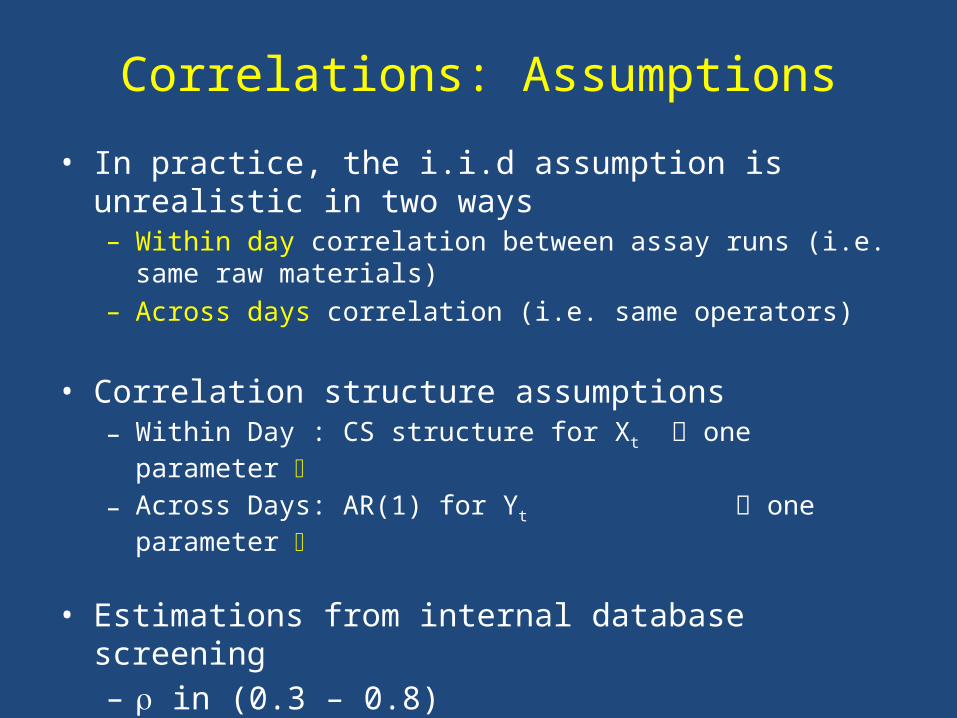
• In practice, the i.i.d assumption is unrealistic in two ways– Within day correlation between assay runs (i.e. same raw materials)– Across days correlation (i.e. same operators)
• Correlation structure assumptions– Within Day : CS structure for Xt one parameter
– Across Days: AR(1) for Yt one parameter
• Estimations from internal database screening– in (0.3 – 0.8)– in (0 – 0.25)

Within-day Correlations : Bounds
EWMA control limits of the average Yt under CS (within-day):
with constant n observations per day and t large
• Need an estimate of (= within-day autocorrelation)• In practice, hardly estimable for each assay (> 300 assays!)
Can standard parameter settings be used?

Within-day Correlations : False AlarmsSimulations assuming no shift in mean
Bounds with = 0 (reality CS = 0, 0.1, 0.2, 0.5)
Bounds with = 0.5 or = 1 (reality CS = 0.5)
Ignoring the correlation structure (=0) strongly increases false alert rates
increases
Assuming maximal correlation ( = 1) decreases false alert rates.. (but Power??)

Within-day Correlations : Power
Reality: Xt ~ CS ( = 0.5)
EWMA bounds with = 0.5 (correct bounds) or = 1
Assuming = 1 :
• « No additional info obtained by repeating test same day »
• Decreases power, but by an acceptable amount as t increases
Simulations assuming shift in mean of 1 SD

Auto-Correlation Across Days
• Control limits of EWMA of the average Yt if Yt ~AR(1) with For full description of f, see Nien Fan Zhang, 1998, Technometrics, vol 40,1 formula (8)
• Note that limits based on are wider than that of ordinary EWMA

Auto-Correlation Across Days: False alerts
Simulations assuming no shift in mean
Bounds with =0.10 or 0.25Reality = 0.10 or 0.25
Bounds with =0Reality = 0.10 or 0.25
Ignoring the correlation structure ( = 0) increases false alert rates compared to true correlation

Auto-Correlation Across Days: PowerSimulations assuming shift in mean = 1SD
Quantifies the time it takes to detect 1SD shift
If correct bounds are used power at 20 days is ~ 60%
(larger bounds)
If bounds = 0 are used, power at 20 days is ~ 80%
Reality Yt is AR(1) with = 0.25 Bounds with =0 and = 0.25

Auto-Correlations Within and Across Days• Reality : within-days = 0.5 and across-days in (0.1, 0.25)• EWMA bounds with =0, = 1
False alarm probability Power at 1SD and 1.3SD
CV=30% :1 SD shift : median 1000 to 13501.3 SD shift : median 1000 to 1500

Back to the example
Estimated = 0.8, =0.2 with n>20, power to detect a shift of 1.3SD > 80%
No autocorrelation structure Bounds with = 1, =0

Summary
• Within-day correlation unknown Use of = 1 in EWMA bounds if in reality <1
– Decreases false alarm rate (compared to ignoring the structure)– Maintains reasonable power if > 0.5
• Across-day correlation unknown Use of = 0 in EWMA bounds if in reality > 0
– Increases the false alarm rate – Small increase of power compared to correct bounds

Take-home message (1/2)
• Correlations exist in data collected for SPC, they should not be ignored
• Theoretical work exists for EWMA charts in the presence of autocorrelations– Important to simulate and present different scenarios to practitioners – Need to understand properties of tool for structure of data at hand

Take-home message (2/2)
• Construct EWMA assuming =0, = 1 for early stage– Limits the false alarm – Need at least 20 days of data to detect shift of 1SD – 1.3SD with
reasonable chance
• When data accumulates (N100), estimate – If non-negligible, use correct bounds or average by week to decrease
correlation across days

Discussion
Thank you for your attention
Any question ?
Acknowledgements
Pierre Cambron (GVCL), Pascal Gérard (GVCL), Hélène Fourmanoir (stat), Jean-Louis Marchal (stat)

References• Montgomery D., Introduction to Statistical Quality Control, Wiley 4th edition 2001• Psarakis S. and Papaleonida G. E. A., SPC Procedures for Monitoring Autocorrelated
Processes, Quality Technology & Quantitative Management Vol. 4, No. 4, pp. 501-540, 2007 • Neubauer A., The EWMA control chart: properties and comparison with other quality-control
procedures by computer simulation, Clinical Chemistry 43:4 594–601 1997 • Shiau J.J.H. and Hsu Y.C., Robustness of the EWMA Control Chart to Non-normality for
Autocorrelated Processes, Quality Technology & Quantitative Management Vol. 2, No. 2, pp. 125-146, 2005
• Han D. and Tsung F., Run Length Properties of the CUSUM and EWMA Schemes for a Stationary Linear Process, Statistica Sinica 19, 473-490 (2009)
• De Vargas, Dias Lopes, Souza, Comparative Study of the Performance of the CUSUM and EWMA Control Charts, Computers & Industrial Engineering 46, 707-724, 2004
• Harris T. and Ross W., Statistical Process Control Procedures for Correlated Observations, The Canadian Journal of Chemical Engineering, 69, 48-57, 1991
• Barger T., Zhou L., Hale M., Moxness M., Swanson S., Chirmule N. Comparing Exponentially Weighted Moving Average and Run Rules in Process Control of Semiquantitative Immunogenicity Immunoassays. The AAPS Journal, 12, 1, 2010