Control 4

PID Control Techniques

Tuning PID Controllers

Finding the values for KP, KI and KD to make

the system behave as desired can be

difficult

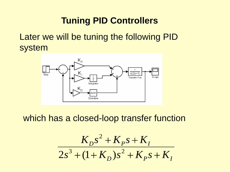
Tuning PID Controllers

Later we will be tuning the following PID

system

IPD

IPD

KsKsKs

KsKsK23

2

)1(2

which has a closed-loop transfer function

Tuning PID Controllers

Changes in the values of the controller

gains move not only the system poles but

also the system zeros.

IPD

IPD

KsKsKs

KsKsK23

2

)1(2

The consequence of this is that adjustment

of a controller gain makes multiple changes

to the system performance some of which

can be undesirable.

Ziegler-Nichols open-loop PID tuning

A step input is applied to the open-loop

system and the response is plotted.

The settings for KP, KI and KD are shown

below

KP KI KD

Proportional only

P/RL

P+I (0.9P)/(RL) 1/(3.33L)

PID (1.2P)/(RL) 1/(2L) 0.5L

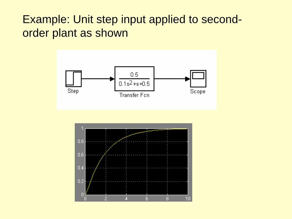
Example: Unit step input applied to second-

order plant as shown

To evaluate the lag, L we’ll run the

sequence over 1 sec

Returning to the 10 sec plot

4.02

8.0RSlope

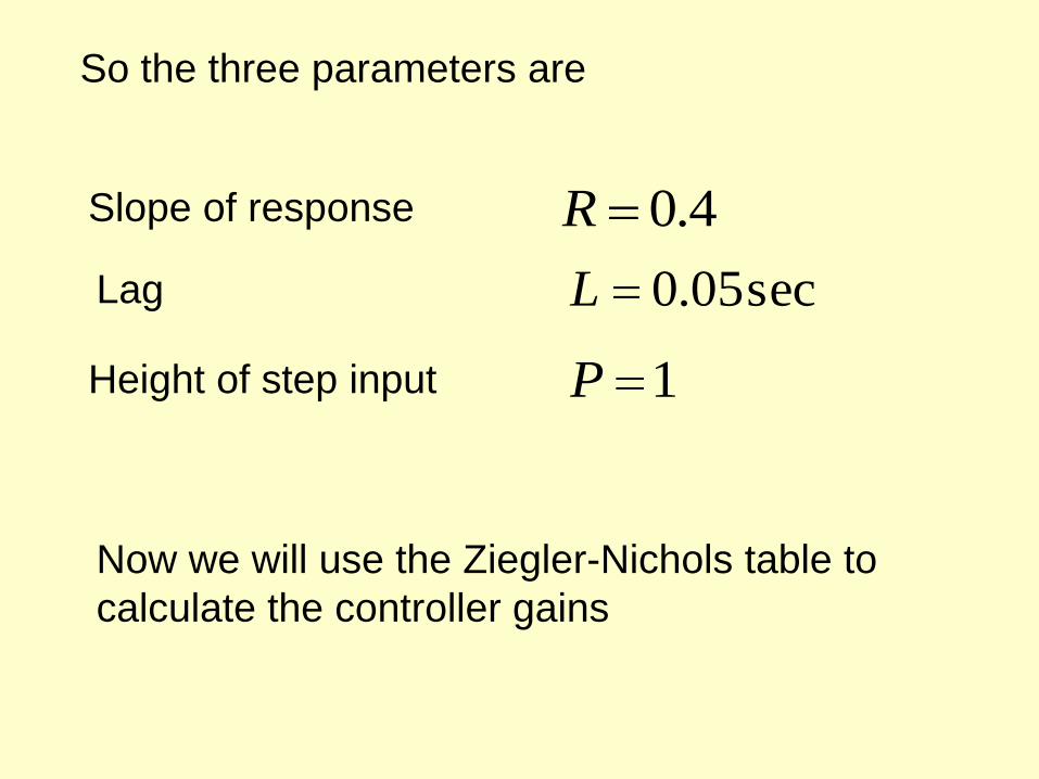
Slope of response 4.0R

sec05.0L

1P

Lag

Height of step input

So the three parameters are

Now we will use the Ziegler-Nichols table to

calculate the controller gains

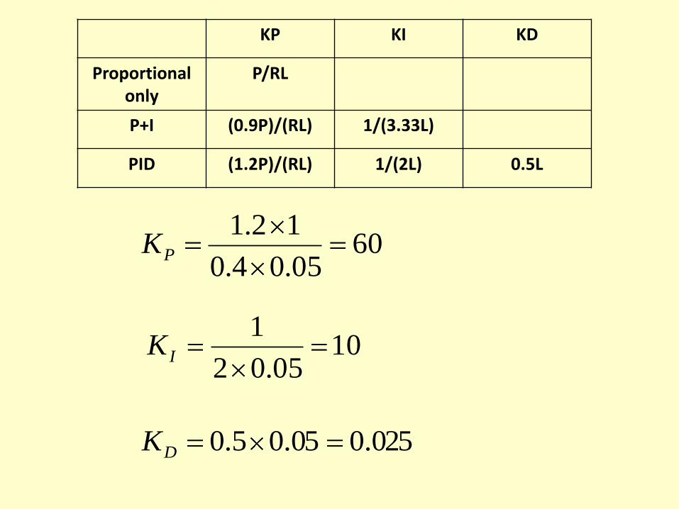
KP KI KD

Proportional only

P/RL

P+I (0.9P)/(RL) 1/(3.33L)

PID (1.2P)/(RL) 1/(2L) 0.5L

6005.04.0

12.1PK

1005.02

1IK

025.005.05.0DK

Putting the plot into a PID control loop

and setting the gains

We get a peak time of 0.2 sec, a 40 %

overshoot, a settling time of 0.8 sec and

zero steady-state error

Increasing the derivative gain KD from 0.025

to 1, halves the overshoot

The Ziegler-Nichols rules can provide a

starting point for further tuning.

The rules do not allow for exact specification of

performance parameters but it is not necessary to

have a system model.

Controller design by pole-placement

Pole placement controller design consists

of calculating the gains to produce a

characteristic equation equivalent to the

desired pole location.

We will start with an example based on a

second-order response

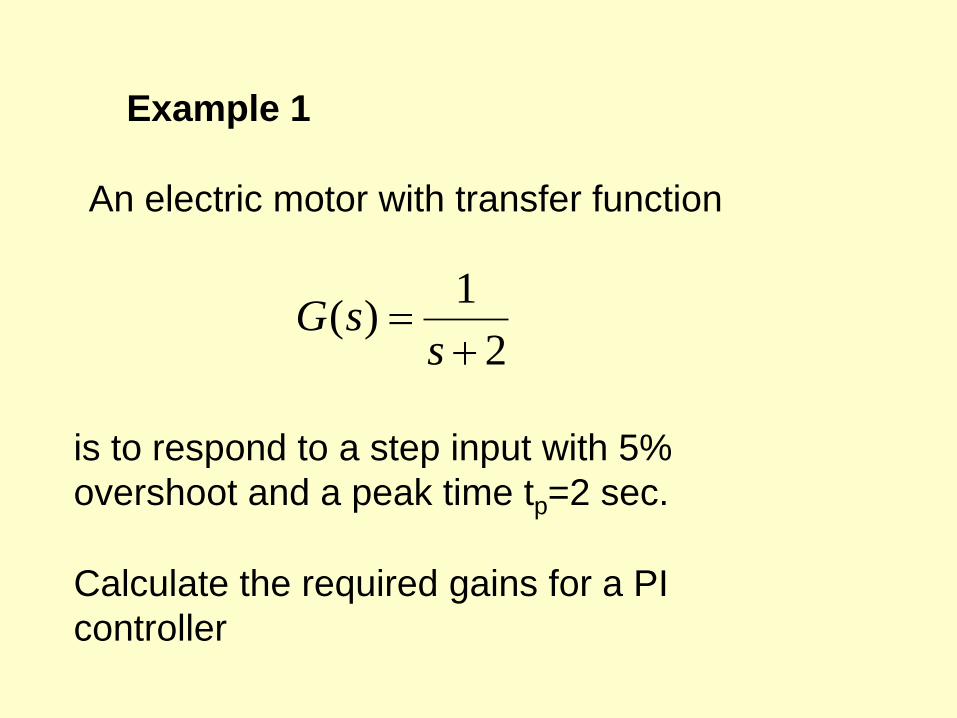
Example 1

An electric motor with transfer function

is to respond to a step input with 5%

overshoot and a peak time tp=2 sec.

2

1)(

ssG

Calculate the required gains for a PI

controller

The required value for ζ

corresponding to a 5%

overshoot is 0.69

The given value of peak time

tp=2 sec

allows us to calculate ωn.

21n

pt

21n

pt

21p

n

t

269.012n

sec/17.2 radn

Inserting these values for ζ and ωn into the

standard second order characteristic equation

02 22

nnss

gives

07.499.22 ss

This is the desired closed-loop characteristic

equation.

The block diagram for the PI controller is shown

below.

The PI section

reduces tos

KK I

P

s

KsK IP

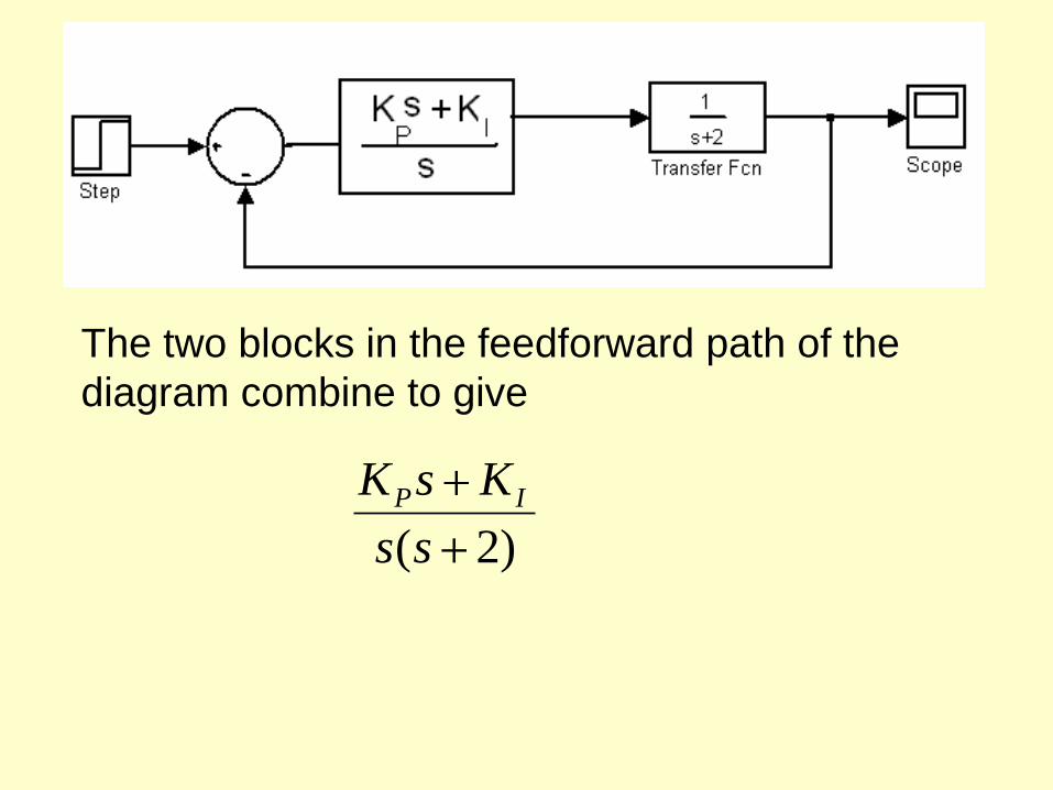
The two blocks in the feedforward path of the

diagram combine to give

)2(ss

KsK IP

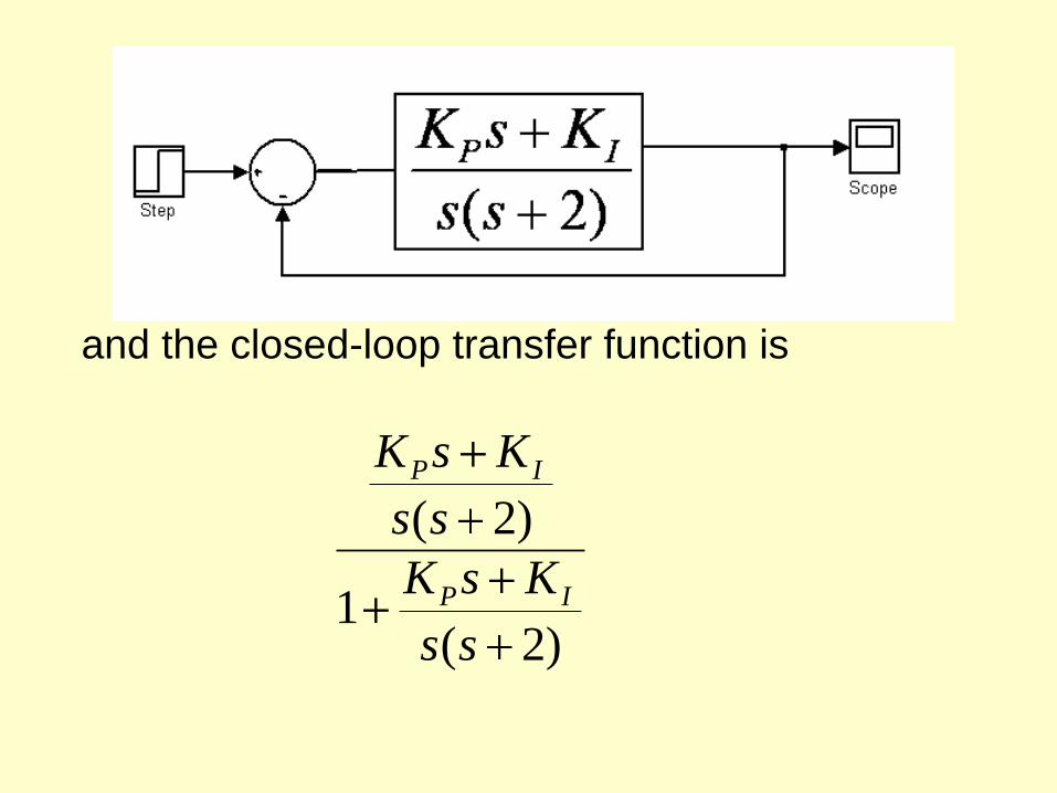
and the closed-loop transfer function is

)2(1

)2(

ss

KsK

ss

KsK

IP

IP

)2(1

)2(

ss

KsK

ss

KsK

IP

IP

IP

IP

KsKss

KsK

)2(

IP

IP

KsKs

KsK

)2(2

IP

IP

KsKs

KsK

)2(2

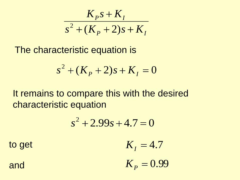
The characteristic equation is

0)2(2

IP KsKs

It remains to compare this with the desired

characteristic equation

07.499.22 ss

to get 7.4IK

and 99.0PK

Entering these values into the block diagram

The peak time ≈ 2 sec and the overshoot =5%

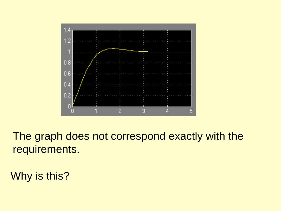
The graph does not correspond exactly with the

requirements.

Why is this?

The required characteristic equation, based on ζ

and ωn is

07.499.22 ss

The corresponding transfer function is

7.499.2

7.42 ss

This goes to 1 in steady state when the output

reaches set point

Putting this transfer function into Simulink

The peak time = 2 sec and the overshoot =5%

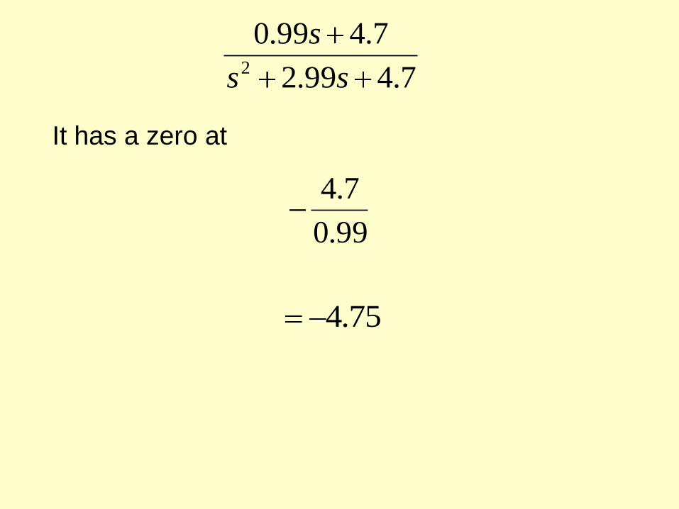
The cltf of the PI controller is

IP

IP

KsKs

KsK

)2(2

7.499.2

7.499.02 ss

s

7.499.2

7.499.02 ss

s

It has a zero at

99.0

7.4

75.4

Putting this transfer function into Simulink

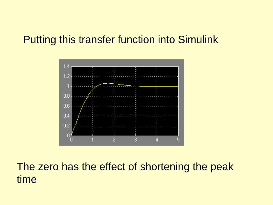
Putting this transfer function into Simulink

The zero has the effect of shortening the peak

time

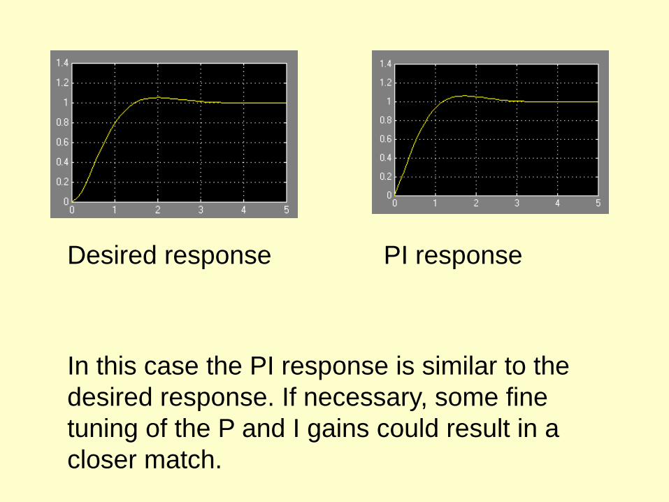
Desired response PI response

In this case the PI response is similar to the

desired response. If necessary, some fine

tuning of the P and I gains could result in a

closer match.

Principles of Controller Design

Controller design in mathematical terms

means the placement of system poles and

zeros

Real poles lead to an

overdamped step

response

Principles of Controller Design

Complex conjugate

poles lead to an

underdamped step

response

Principles of Controller Design

Closed-loop zeros

may cause

overshoot, even if

the system is

overdamped

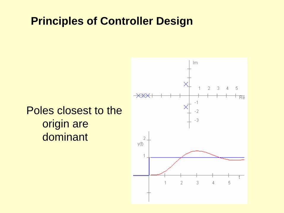
Principles of Controller Design

Poles closest to the

origin are

dominant

Example 2

Design a PID controller for a plant with transfer

function

)12(

1)(

sssG

The peak time is to be 2 sec and the overshoot

5%

The system block diagram is shown below

We can try the open-loop Ziegler Nichols method

but the system is open-loop unstable, so it

doesn’t work.

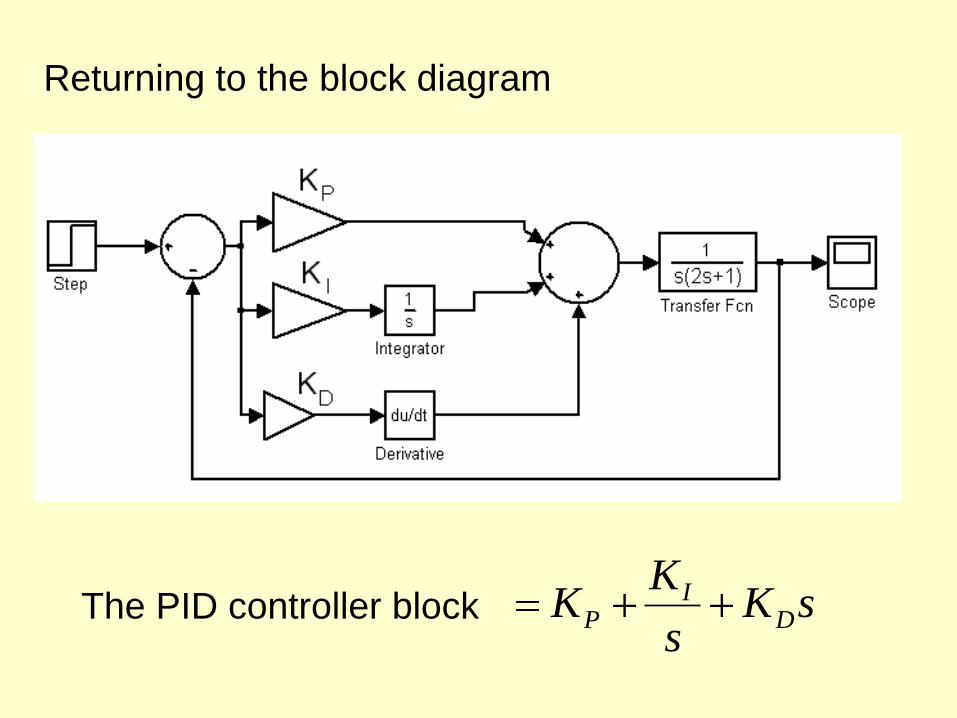
Returning to the block diagram

The PID controller block sKs

KK D

IP

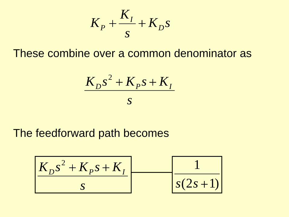
These combine over a common denominator as

sKs

KK D

IP

s

KsKsK IPD

2

The feedforward path becomes

s

KsKsK IPD

2

)12(

1

ss

s

KsKsK IPD

2

)12(

1

ss

and these combine in series to form

)12(2

2

ss

KsKsK IPD

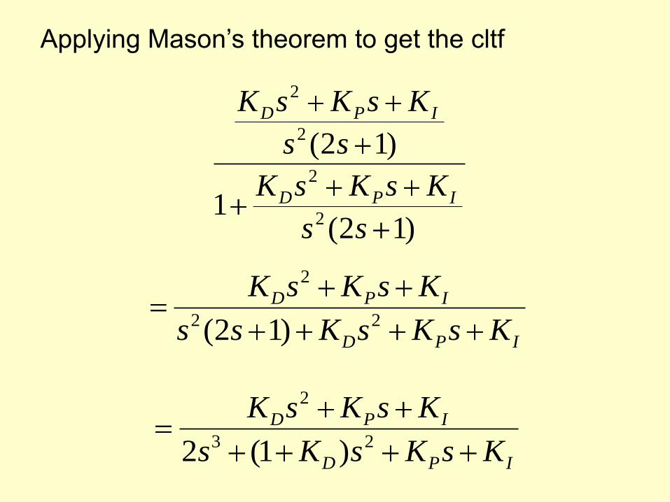
Applying Mason’s theorem to get the cltf

)12(1

)12(

2

2

2

2

ss

KsKsK

ss

KsKsK

IPD

IPD

IPD

IPD

KsKsKss

KsKsK22

2

)12(

IPD

IPD

KsKsKs

KsKsK23

2

)1(2

IPD

IPD

KsKsKs

KsKsK23

2

)1(2

The system characteristic equation is

0)1(2 23

IPD KsKsKs

There are also two system zeros located at the

roots of the numerator equation

02

IPD KsKsK

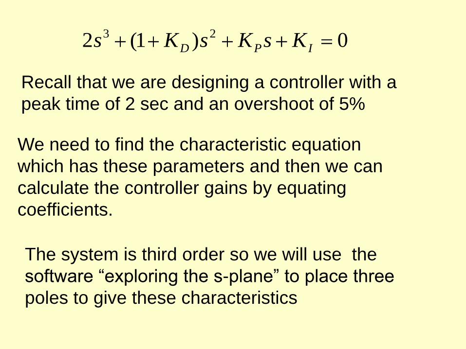
We need to find the characteristic equation

which has these parameters and then we can

calculate the controller gains by equating

coefficients.

Recall that we are designing a controller with a

peak time of 2 sec and an overshoot of 5%

0)1(2 23

IPD KsKsKs

The system is third order so we will use the

software “exploring the s-plane” to place three

poles to give these characteristics

The poles are located at

,8.1

3.23.1 jand

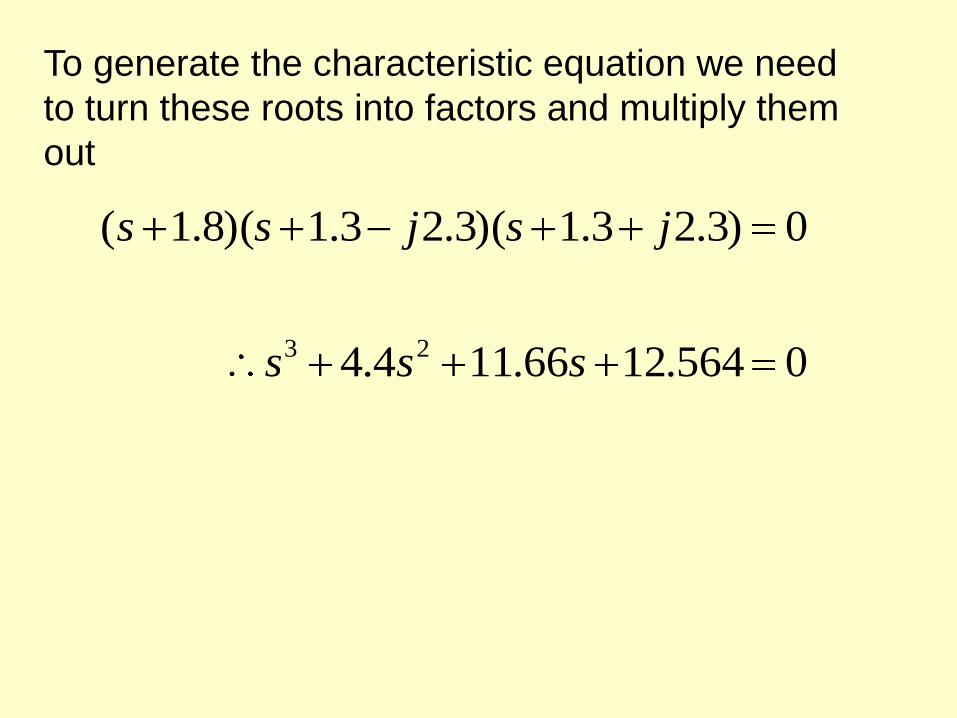
To generate the characteristic equation we need

to turn these roots into factors and multiply them

out

0)3.23.1)(3.23.1)(8.1( jsjss

0564.1266.114.4 23 sss

0564.1266.114.4 23 sss

Now we compare this equation with the

controller characteristic equation

0)1(2 23

IPD KsKsKs

The coefficients of s3 need to be equal so we’ll

multiply the top equation by 2

0128.2532.238.82 23 sss

128.25IK

32.23PK

8.7DK

0)1(2 23

IPD KsKsKs

0128.2532.238.82 23 sss

Putting these gain values into the PID controller

The overshoot is ~ 40% and the peak time ~1 sec

02

IPD KsKsK

The zeros in the numerator of the cltf are increasing

the overshoot so further tuning is required.

We will finish by attempting instead to tune the

system using the Ziegler-Nichols closed-loop

method described in the Control 3 lecture.

1. SET KP. Starting with KP=0, KI=0 and KD=0,

increase KP until the output starts overshooting

and oscillating significantly.

2. Reduce KP to 75% of the value established in

step 1.

3. SET KD. Increase KD until the overshoot is

reduced to an acceptable level

4. SET KI. Increase KI until the final error is

equal to zero.

Recall the rules for the modified Ziegler-Nichols

closed-loop method

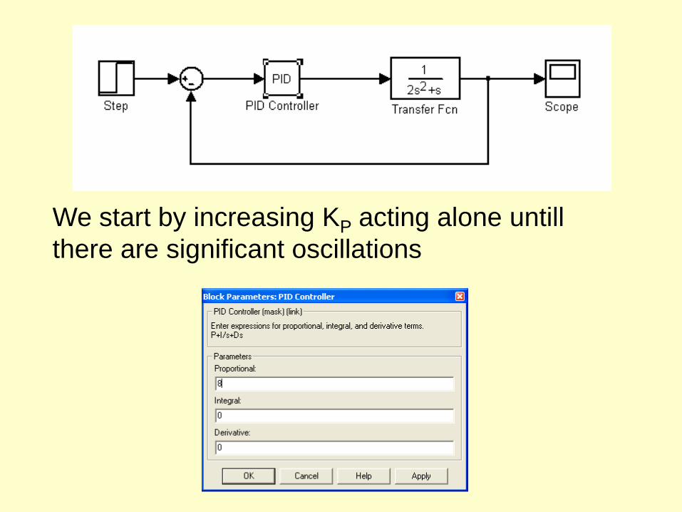
We start by increasing KP acting alone untill

there are significant oscillations

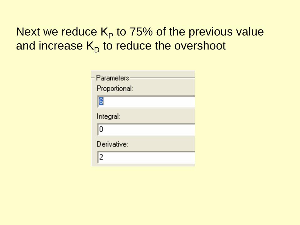
Next we reduce KP to 75% of the previous value

and increase KD to reduce the overshoot

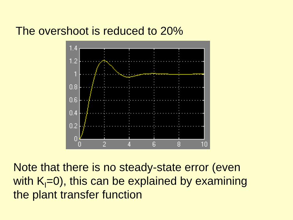
The overshoot is reduced to 20%

Note that there is no steady-state error (even

with KI=0), this can be explained by examining

the plant transfer function

12

12 ss

The cltf

which1 in steady state for a unit step input

12

11

)12(

1

ssss

Viewing this mathematically, the plant transfer

function

already contains an integrator.

Controller tuning strategies

1. Modified Ziegler-Nichols closed-loop

2. Ziegler-Nichols open-loop

3. pole placement

4. trial and error

Whatever method is employed, some further fine

tuning is required . Sometimes the desired

response cannot be achieved for the given plant

and controller.