
Contributions to high-dimensional data analysis : some ...€¦ · high-dimensional data analysis:...
140
Copyright is owned by the Author of the thesis. Permission is given for a copy to be downloaded by an individual for the purpose of research and private study only. The thesis may not be reproduced elsewhere without the permission of the Author.
Transcript of Contributions to high-dimensional data analysis : some ...€¦ · high-dimensional data analysis:...

Copyright is owned by the Author of the thesis. Permission is given for a copy to be downloaded by an individual for the purpose of research and private study only. The thesis may not be reproduced elsewhere without the permission of the Author.

Contributions tohigh-dimensional data analysis:
some applications of theregularized covariance matrices
A thesis submitted in partial fulfilment of the requirements for the
degree of
Doctor of Philosophy
in
Statistics
at Massey University, Albany
New Zealand.
Insha ULLAH
March 2015

i
Abstract
High-dimensional data sets, particularly those where the number of variables ex-
ceeds the number of observations, are now common in many subject areas includ-
ing genetics, ecology, and statistical pattern recognition to name but a few. The
sample covariance matrix becomes rank deficient and is not invertible when the
number of variables are more than the number of observations. This poses a se-
rious problem for many classical multivariate techniques that rely on an inverse
of a covariance matrix. Recently, regularized alternatives to the sample covari-
ance have been proposed, which are not only guaranteed to be positive definite
but also provide reliable estimates. In this Thesis, we bring together some of the
important recent regularized estimators of the covariance matrix and explore their
performance in high-dimensional scenarios via numerical simulations. We make
use of these regularized estimators and attempt to improve the performance of the
three classical multivariate techniques in high-dimensional settings.
In a multivariate random effects models, estimating the between-group covariance
is a well known problem. Its classical estimator involves the difference of two
mean square matrices and often results in negative elements on the main diago-
nal. We use a lasso-regularized estimate of the between-group mean square and
propose a new approach to estimate the between-group covariance based on the
EM-algorithm. Using simulation, the procedure is shown to be quite effective and
the estimate obtained is always positive definite.

ii
Multivariate analysis of variance (MANOVA) face serious challenges due to the un-
desirable properties of the sample covariance in high-dimensional problems. First,
it suffer from low power and does not maintain accurate type-I error when the
dimension is large as compared to the sample size. Second, MANOVA relies on
the inverse of a covariance matrix and fails to work when the number of variables
exceeds the number of observation. We use an approach based on the lasso reg-
ularization and present a comparative study of the existing approaches including
our proposal. The lasso approach is shown to be an improvement in some cases,
in terms of power of the test, over the existing high-dimensional methods.
Another problem that is addressed in the Thesis is how to detect unusual future
observations when the dimension is large. The Hotelling T 2 control chart has
traditionally been used for this purpose. The charting statistic in the control chart
rely on the inverse of a covariance matrix and is not reliable in high-dimensional
problems. To get a reliable estimate of the covariance matrix we use a distribution
free shrinkage estimator. We make use of the available baseline set of data and
propose a procedure to estimate the control limits for monitoring the individual
future observations. The procedure do not assume multivariate normality and
seems robust to the violation of multivariate normality. The simulation study
shows that the new method performs better than the traditional Hotelling T 2
control charts.

Acknowledgements
My Ph.D project was supported by Higher Education Commission (HEC) of Pak-
istan. I gratefully acknowledge the financial support of the HEC.
I am grateful to my supervisor, Dr. Beatrix Jones for being my supervisor. She
gave me the opportunity to learn from her and work together with her. Indeed,
it is because of her, I managed to accomplish the task. Thanks Beatrix for your
constant support, patience, suggestions and constructive criticisms. You made it
a fruitful journey for me. I would like to thank my co-supervisor Prof. James
Curran for his valuable feedbacks.
I have greatly benefited from the group of statistician working at the Institute of
Natural and Mathematical Sciences, Massey University. I would like to thank all
members of the group.
I also acknowledge the support of my family and friends. Thanks to Hoor and
Hamood for being patient with me.
iii

Contents
Abstract i
Acknowledgements iii
List of Figures vi
List of Tables xiii
1 Introduction 1
1.1 Introduction . . . . . . . . . . . . . . . . . . . . . . . . . . . . . . . 1
2 Regularized estimation of high-dimensional covariance matrices 5
2.1 Introduction . . . . . . . . . . . . . . . . . . . . . . . . . . . . . . . 5
2.2 Moore-Penrose generalized inverse . . . . . . . . . . . . . . . . . . . 6
2.3 Shrinkage Estimate . . . . . . . . . . . . . . . . . . . . . . . . . . . 7
2.3.1 Computation of the shrinkage intensity ρ . . . . . . . . . . . 8
2.4 Penalized Normal Likelihood . . . . . . . . . . . . . . . . . . . . . . 10
2.4.1 Ridge Regularization . . . . . . . . . . . . . . . . . . . . . . 11
2.4.1.1 Selection of the ridge parameter ρ . . . . . . . . . . 11
2.4.2 Lasso Regularization . . . . . . . . . . . . . . . . . . . . . . 12
2.4.3 Adaptive lasso and SCAD penalty functions . . . . . . . . . 14
2.4.4 Choosing the optimal value of the penalty parameter ρ . . . 16
2.5 Numerical simulations . . . . . . . . . . . . . . . . . . . . . . . . . 18
2.6 Summary and conclusion . . . . . . . . . . . . . . . . . . . . . . . . 22
2.7 Contributions of the Chapter . . . . . . . . . . . . . . . . . . . . . 23
3 Hierarchical covariance estimation 28
3.1 Introduction . . . . . . . . . . . . . . . . . . . . . . . . . . . . . . . 28
3.2 Hierarchical covariance estimation via EM algorithm . . . . . . . . 31
3.3 Applications . . . . . . . . . . . . . . . . . . . . . . . . . . . . . . . 33
3.3.1 Numerical experiments . . . . . . . . . . . . . . . . . . . . . 34
3.3.2 Real data example . . . . . . . . . . . . . . . . . . . . . . . 45
3.4 Conclusion . . . . . . . . . . . . . . . . . . . . . . . . . . . . . . . . 48
3.5 Contributions of the Chapter . . . . . . . . . . . . . . . . . . . . . 49
iv

Contents v
4 Regularized MANOVA for high-dimensional data 50
4.1 Introduction . . . . . . . . . . . . . . . . . . . . . . . . . . . . . . . 50
4.2 Previous works . . . . . . . . . . . . . . . . . . . . . . . . . . . . . 53
4.3 LASSO Regularization . . . . . . . . . . . . . . . . . . . . . . . . . 56
4.3.1 Selection of ρ . . . . . . . . . . . . . . . . . . . . . . . . . . 56
4.4 Simulation study . . . . . . . . . . . . . . . . . . . . . . . . . . . . 57
4.4.1 Simulation results . . . . . . . . . . . . . . . . . . . . . . . . 59
4.5 Practical application . . . . . . . . . . . . . . . . . . . . . . . . . . 66
4.6 Conclusion and discussion . . . . . . . . . . . . . . . . . . . . . . . 69
4.7 Contributions of the Chapter . . . . . . . . . . . . . . . . . . . . . 70
5 Monitoring future observations in the high-dimensional setting 72
5.1 Introduction . . . . . . . . . . . . . . . . . . . . . . . . . . . . . . . 72
5.2 Shrinkage estimate of a covariance matrix . . . . . . . . . . . . . . 75
5.3 Proposed procedure . . . . . . . . . . . . . . . . . . . . . . . . . . . 80
5.4 Simulation study . . . . . . . . . . . . . . . . . . . . . . . . . . . . 82
5.5 The in-control run length performance . . . . . . . . . . . . . . . . 86
5.6 Practical applications . . . . . . . . . . . . . . . . . . . . . . . . . . 87
5.6.1 Example 1: Gene expression data . . . . . . . . . . . . . . . 87
5.6.2 Example 2: Chemical process data . . . . . . . . . . . . . . 92
5.7 Summary and Conclusion . . . . . . . . . . . . . . . . . . . . . . . 96
5.8 Contributions of the Chapter . . . . . . . . . . . . . . . . . . . . . 97
6 General Conclusions 100
6.1 Regularized estimation of the high-dimensional covariance matrices 101
6.2 Hierarchical covariance estimation . . . . . . . . . . . . . . . . . . . 101
6.3 Regularized MANOVA for high-dimensional data . . . . . . . . . . 102
6.4 Monitoring individual future observations in the high-dimensionalsetup . . . . . . . . . . . . . . . . . . . . . . . . . . . . . . . . . . . 103
6.5 Commonalities and future work . . . . . . . . . . . . . . . . . . . . 104
A Supplementary Figure for Chapter 4 106
B Supplementary Figure for Chapter 5 109
C DRC forms 118
References 119

List of Figures
2.1 A schematic diagram showing the regularized estimates against themaximum likelihood estimates for the elements of the inverse co-variance matrix (a) the ridge, (b) the lasso, (c) the adaptive lasso,(d) the SCAD regularized estimates. . . . . . . . . . . . . . . . . . 16
2.2 Off-diagonal elements of simulated correlation matrices for p = 20using the algorithm of Schafer & Strimmer (2005a). The proportionof non-zero off-diagonal elements in step 2 of the algorithm is (a)20%, (b) 30%, and (c) 40%. For a fixed value of p as we increase theproportion of the non-zero elements in the off-diagonal positions, thesize of the off-diagonal elements in the correlation matrix decreases. 21
2.3 Ordered eigenvalues of a true and estimated covariance matrices.A true covariance matrix is generated using the random methodwith proportion of non-zero off-diagonal elements equals to 50%and p = 40. The covariance matrix is estimated 1000 times, using1000 samples for each n ∈ 20, 40, 1000 from a multivariate normaldistribution and the average eigenvalues of the estimated covariancematrices are presented. The diagonal elements of the estimatedcovariance matrices are not penalized in any of the regularizationprocedures. . . . . . . . . . . . . . . . . . . . . . . . . . . . . . . . 24
2.4 An exchangeable covariance structure is used with b = 0.6. Thebox-plots show the distributions of the three loss functions for thefive competing procedures. The three loss functions are calculatedfor each of 1000 samples of size n = 20 from a multivariate normaldistribution with p ∈ 10, 20, 40, 80. Since the shrinkage, lasso,adaptive lasso, and SCAD regularization allow to penalize the di-agonal, the diagonal elements in (a) are left unpenalized while in(b) they are penalized for all the four methods. As ridge regular-ization does not allow to penalize the diagonal elements; therefore,the distributions in (b) are the replicates of the results in (a) forridge regularization. . . . . . . . . . . . . . . . . . . . . . . . . . . . 25
vi

List of Figures vii
2.5 A random covariance structure is used with the proportion of non-zero edges equals to 50%, 30%, 20%, and 10%, respectively, for pequals to 10, 20, 40, and 80. The box-plots show the distributions ofthe three loss functions for the five competing procedures. The threeloss functions are calculated for each of 1000 samples of size n = 20from a multivariate normal distribution with p ∈ 10, 20, 40, 80.Since the shrinkage, lasso, adaptive lasso, and SCAD regularizationallow to penalize the diagonal, the diagonal elements in (a) are leftunpenalized while in (b) they are penalized for all the four meth-ods. As ridge regularization does not allow to penalize the diagonalelements; therefore, the distributions in (b) are the replicates of theresults in (a) for ridge regularization. . . . . . . . . . . . . . . . . 26
2.6 An AR(1) covariance structure is used with b = 0.6. The box-plotsshow the distributions of the three loss functions for the five com-peting procedures. The three loss functions are calculated for eachof 1000 samples of size n = 20 from a multivariate normal distribu-tion with p ∈ 10, 20, 40, 80. Since the shrinkage, lasso, adaptivelasso, and SCAD regularization allow to penalize the diagonal, thediagonal elements in (a) are left unpenalized while in (b) they arepenalized for all the four methods.As ridge regularization does notallow to penalize the diagonal elements; therefore, the distributionsin (b) are the replicates of the results in (a) for ridge regularization. 27
3.1 Simulated data on first two principle components for the three cases(a) easiest, (c) moderate, and (e) hard. . . . . . . . . . . . . . . . 35
3.2 Typical cross-validation scores obtained over the first five iterationsof the proposed EM algorithm. We use 100% non-zero off-diagonalelements in U−1 and C−1. The elements of U are of a moderatesize. In (a) p = 5, m = 10, r = 5 and in (b) p = 15, m = 10, r = 5. 37
3.3 Estimates of different elements of the between-group covariance ma-trix in an easy case. Each box-plot is made up of 1000 estimatesof the same element using 1000 different data sets. The gray boxesrepresent the estimate of five diagonal elements and the horizontalline in each panel represents the true value. . . . . . . . . . . . . . . 39
3.4 Estimates of different elements of the between-group covariance ma-trix in a moderate case. Each box-plot is made up of 1000 estimatesof the same element using 1000 different data sets. The gray boxesrepresent the estimate of the five diagonal elements and the hori-zontal line in each panel represents the true value. . . . . . . . . . . 40
3.5 Estimates of different elements of the between-group covariance ma-trix in a hard case. Each box-plot is made up of 1000 estimates ofthe same element using 1000 different data sets. The gray boxesrepresent the estimate of five diagonal elements and the horizontalline in each panel represents the true value. . . . . . . . . . . . . . . 41

List of Figures viii
3.6 The distributions of the estimated eigenvalues of a between-groupcovariance matrix with 1000 different data sets. We use C as in(3.17) and U in (3.15) is scaled to the easy case: (a) m = 10 andr = 5, (b) m = 10 and r = 20, (c) m = 30 and r = 5, and (d)m = 30 and r = 20. See the mean squared errors of the estimatedeigenvalues in Table 3.1. . . . . . . . . . . . . . . . . . . . . . . . . 43
3.7 The distributions of the estimated eigenvalues of a between-groupcovariance matrix with 1000 different data sets. We use C as in(3.17) and U in (3.15) is scaled to the moderate case: (a) m = 10and r = 5, (b) m = 10 and r = 20, (c) m = 30 and r = 5, and (d)m = 30 and r = 20. See the mean squared errors of the estimatedeigenvalues in Table 3.2. . . . . . . . . . . . . . . . . . . . . . . . . 44
3.8 The distributions of the estimated eigenvalues of a between-groupcovariance matrix with 1000 different data sets. We use C as in(3.17) and U in (3.15) is scaled to the hard case: (a) m = 10 andr = 5, (b) m = 10 and r = 20, (c) m = 30 and r = 5, and (d)m = 30 and r = 20. See the mean squared errors of the estimatedeigenvalues in Table 3.3. . . . . . . . . . . . . . . . . . . . . . . . . 45
3.9 First two principle components of glass chemical composition data. 48
4.1 Distribution of the sum of absolute errors (∑p
i=1
∣∣∣λi − λi∣∣∣ /∑p
i=1 λi)
in the estimated eigenvalues under (a) exchangeable and (b) AR(1)covariance structures both with b = 0.6. For each value of p ∈10, 20, 40, 80, 1000 samples of size 20 are simulated from a mul-tivariate normal distribution. Eigenvalues of the true covariancematrix are estimated using shrinkage, ridge, and lasso regulariza-tion and the sum of absolute errors are calculated for each of the1000 samples. Note that, the estimation error increases as we in-crease p and the lasso regularization maintains the highest accuracy.. . . . . . . . . . . . . . . . . . . . . . . . . . . . . . . . . . . . . . 61
4.2 Power comparison of MANOVA test based on 5 competing proce-dures under AR(1) covariance structure with b = 0.4. For eachvalue of p ∈ [2, 30], the point on a power curve is the average of1000 experiments. The significance level is 0.05. . . . . . . . . . . . 62
4.3 Power comparison of MANOVA test based on 5 competing proce-dures under AR(1) covariance structure with b = 0.8. For eachvalue of p ∈ [2, 30], the point on a power curve is the average of1000 experiments. The significance level is 0.05. . . . . . . . . . . . 63
4.4 Power comparison of MANOVA test based on 5 competing proce-dures under exchangeable covariance structure with b = 0.4. Foreach value of p ∈ [2, 30], the point on a power curve is the averageof 1000 experiments. The significance level is 0.05. . . . . . . . . . 64
4.5 Power comparison of MANOVA test based on 5 competing proce-dures under exchangeable covariance structure with b = 0.7. Foreach value of p ∈ [2, 30], the point on a power curve is the averageof 1000 experiments. The significance level is 0.05. . . . . . . . . . 65

List of Figures ix
4.6 Time comparison of 3 competing regularization procedures undertwo different covariance structures: exchangeable and AR(1). Eachpoint in the graph is averaged over 10 replicates. The covariancestructure does not make big difference in computational time forridge and shrinkage therefore only shown for exchangeable. Thecomputational time for principal components and and generalizedinverse is not shown but lie below the shrinkage estimate. . . . . . . 66
4.7 Serial correlation coefficients of soil compaction at shallower depthswith soil compaction at all the deeper depths after adjusting forgroup means. Each sequence of joined points of the same colorrepresents the correlation of the measurements at a certain depthwith the measurements at deeper levels (with the depth value givenon the x axis). Note that for each of the 18 depths (variables) wehave 21 observations. . . . . . . . . . . . . . . . . . . . . . . . . . . 68
4.8 Projection of the data (variables are standardized to have zeromeans and unite standard deviations) onto the first two principalcomponents of the data after adjusting for group means. . . . . . . 69
5.1 Ordered eigenvalues of a shrinkage estimate, Σρ, in comparison withthe eigenvalues of a true covariance, Σ, and the sample covariancematrix, S. Σ is of AR(1) structure with b = 0.5, and S and Σρ arecalculated from a sample of size n = 25 drawn from a multivariate(p = 20) normal distribution with µ = 0 and covariance matrix Σ. . 78
5.2 A hypothetical diagram illustrating the shrinkage effect for bivari-ate data (Warton, 2008). The lines are the 99% probability con-tours based on the true covariance (the solid lines) and shrunkencovariance (the dashed lines). The shrinkage estimate reduces theeccentricity of the ellipse (the ellipse represented by solid black lineis squashed along the major axis and make the ellipse representedby dashed line). The diagram also illustrates how the shift in differ-ent orientation can effect the power of a method to detect it. Thered ellipse shows the shifted true distribution. It is shifted alongthe (a) first eigenvector (b) along second eigenvector. A larger shiftis required along the first eigenvector to be detected as comparedto the shift along second eigenvector. Note that “detected” meansthose red points that are outside the black ellipses. . . . . . . . . . 79
5.3 Power (solid lines) and false alarm rate (dashed lines) for AR(1)covariance structure. The black lines are based on the true parame-ters and therefore are the best possible results one can achieve. Thegreen lines are the results for the Hotelling T 2 control chart (usessample covariance matrix) and the blue lines are the results fromnew method. . . . . . . . . . . . . . . . . . . . . . . . . . . . . . . 84

List of Figures x
5.4 Power (solid lines) and false alarm rate (dashed lines) for exchange-able covariance structure. The black lines are based on the true pa-rameters and therefore are the best possible results one can achieve.The green lines are the results for the Hotelling T 2 control chart(uses sample covariance matrix) and the blue lines are the resultsfrom new method. . . . . . . . . . . . . . . . . . . . . . . . . . . . 85
5.5 First two principle components of the gene expression data. All out-of-control points in Figure 5.6 (including 12 out-of control pointsfrom baseline set of data) are encircled. . . . . . . . . . . . . . . . . 91
5.6 Multivariate control chart using study 1 data as a baseline set ofdata (black) and study 2 as a future set of data (red). The solidline at T 2 = 853.504 represent the UCL at 5% level of significance. . 92
5.7 Principal components trajectory plot for the chemical process datawith 99% confidence ellipse. Only the first 20 baseline observationsare used to compute the principal components. The 10 future ob-servation are plotted with star symbols and are numbered from 21to 30 in order to show the natural sequence of the points. . . . . . 93
5.8 Control chart produced by the proposed method for monitoring thechemical process data shown in Figure 5.7. The first 20 obser-vations are used to estimate the control limits. The solid line atT 2 = 11.1887 indicates the control limit of the chart at 1% level ofsignificance. . . . . . . . . . . . . . . . . . . . . . . . . . . . . . . 94
5.9 Principal components trajectory plot for the chemical process datawith 99% confidence ellipse. Note that the first 10 baseline observa-tions are dropped from the analysis and the principal componentsare computed from the middle 10 observations. The last 10 obser-vations are plotted with star symbols and are numbered from 21 to30 in order to show the natural sequence of the points. . . . . . . . 95
5.10 Control chart produced by the proposed method for monitoring thechemical process data shown in Figure 5.9. Only the middle 10 ob-servations are used to estimate the empirical reference distribution.The solid line at T 2 = 13.1733 indicates the control limit of thechart at at 1% level of significance. . . . . . . . . . . . . . . . . . . 96
A.1 Power comparison of MANOVA test based on 5 competing proce-dures under AR(1) covariance structure with b = 0.4. For eachvalue of p ∈ [2, 30], the power is estimated using 1000 samples andthe significance level is kept as 0.05. . . . . . . . . . . . . . . . . . . 107
A.2 Power comparison of MANOVA test based on 5 competing proce-dures under exchangeable covariance structure with b = 0.4. Foreach value of p ∈ [2, 30], the power is estimated using 1000 samplesand the significance level is kept as 0.05. . . . . . . . . . . . . . . . 108

List of Figures xi
B.1 Power (solid lines) and false alarm rate (dashed lines) for AR(1)covariance structure with b = 0.3. The black lines are based on thetrue parameters and therefore are the best possible results one canachieve. The green lines are the results for standard method (usingsample mean and sample covariance matrix) and the blue lines arethe results from new method. . . . . . . . . . . . . . . . . . . . . . 110
B.2 Power (solid lines) and false alarm rate (dashed lines) for AR(1)covariance structure with b = 0.4. The black lines are based on thetrue parameters and therefore are the best possible results one canachieve. The green lines are the results for standard method (usingsample mean and sample covariance matrix) and the blue lines arethe results from new method. . . . . . . . . . . . . . . . . . . . . . 111
B.3 Power (solid lines) and false alarm rate (dashed lines) for AR(1)covariance structure with b = 0.6. The black lines are based on thetrue parameters and therefore are the best possible results one canachieve. The green lines are the results for standard method (usingsample mean and sample covariance matrix) and the blue lines arethe results from new method. . . . . . . . . . . . . . . . . . . . . . 112
B.4 Power (solid lines) and false alarm rate (dashed lines) for AR(1)covariance structure with b = 0.7. The black lines are based on thetrue parameters and therefore are the best possible results one canachieve. The green lines are the results for standard method (usingsample mean and sample covariance matrix) and the blue lines arethe results from new method. . . . . . . . . . . . . . . . . . . . . . 113
B.5 Power (solid lines) and false alarm rate (dashed lines) for exchange-able covariance structure with b = 0.3. The black lines are based onthe true parameters and therefore are the best possible results onecan achieve. The green lines are the results for standard method(using sample mean and sample covariance matrix) and the bluelines are the results from new method. . . . . . . . . . . . . . . . . 114
B.6 Power (solid lines) and false alarm rate (dashed lines) for exchange-able covariance structure with b = 0.4. The black lines are based onthe true parameters and therefore are the best possible results onecan achieve. The green lines are the results for standard method(using sample mean and sample covariance matrix) and the bluelines are the results from new method. . . . . . . . . . . . . . . . . 115
B.7 Power (solid lines) and false alarm rate (dashed lines) for exchange-able covariance structure with b = 0.6. The black lines are based onthe true parameters and therefore are the best possible results onecan achieve. The green lines are the results for standard method(using sample mean and sample covariance matrix) and the bluelines are the results from new method. . . . . . . . . . . . . . . . . 116

List of Figures xii
B.8 Power (solid lines) and false alarm rate (dashed lines) for exchange-able covariance structure with b = 0.7. The black lines are based onthe true parameters and therefore are the best possible results onecan achieve. The green lines are the results for standard method(using sample mean and sample covariance matrix) and the bluelines are the results from new method. . . . . . . . . . . . . . . . . 117

List of Tables
3.1 Mean squared errors of the estimated eigenvalues presented in Fig-ure 3.6. . . . . . . . . . . . . . . . . . . . . . . . . . . . . . . . . . . 46
3.2 Mean squared errors of the estimated eigenvalues presented in Fig-ure 3.7. . . . . . . . . . . . . . . . . . . . . . . . . . . . . . . . . . . 46
3.3 Mean squared errors of the estimated eigenvalues presented in Fig-ure 3.8. . . . . . . . . . . . . . . . . . . . . . . . . . . . . . . . . . . 47
4.1 Values of the shift parameter, δ, used in the simulation study toobtain a moderate power. . . . . . . . . . . . . . . . . . . . . . . . 62
4.2 Table of p-values for five competing procedures. Significant effectsat α = 0.05 are shown in bold. . . . . . . . . . . . . . . . . . . . . 68
5.1 In-control median run length (MRL) under both the AR(1) struc-ture of covariance and the exchangeable structure of covariance withb = .6 (the lower and upper quartiles are shown inside the parenthe-ses). The desired MRL is the median of the geometric distributionwith parameter α. The size of the baseline set of data is 50. . . . . 88
5.2 In-control median run length (MRL) under both the AR(1) struc-ture of covariance and the exchangeable structure of covariance withb = .6 (the lower and upper quartiles are shown inside the parenthe-ses). The desired MRL is the median of the geometric distributionwith parameter α. The size of the baseline set of data is 100. . . . . 89
5.3 Chemical process data. There are total 30 observations. The first20 observations constitute the baseline set of data and the last 10observations are the new observations used for testing and monitoring. 99
A.1 Values of the shift parameter, δ, used in the simulation experimentswhose results are presented in Figure A.1 and Figure A.2. . . . . . . 106
xiii

Chapter 1
Introduction
1.1 Introduction
High-dimensional data, particularly those where the number of observed variable,
p, is greater than the sample size, n, is becoming increasingly prevalent in many
subject areas. For example, because of the high-throughput technology, a greater
number of features can be observed in a microarray data set whereas the sample
size cannot be increased. In this kind of high-dimensional data set, the sample
covariance is either not invertible (if n < p) because of its rank deficiency; or,
the inverse of a covariance matrix is unstable (n is comparable to p) and is not
reliable.
The situation is challenging to any multivariate statistical procedure, especially
those that rely on the inverse of the covariance matrix, and has attracted the atten-
tion of many researchers in the recent years. Regularized procedures for estimating
the covariance matrix have been proposed. These include ridge regularization; the
shrinkage method that shrinks the sample covariance towards a target; and the
lasso regularization among others. These regularized estimates are not only guar-
anteed to be positive definite (even when n < p) but have also been proven to be
more reliable than the sample covariance when n is comparable to p. However,
it has been only recently that the regularized covariance matrix is used as an in-
gredient in other statistical techniques. In this Thesis, we bring together some of
the important high-dimensional covariance estimation methodologies and extend
their utility to three different multivariate statistical techniques. The contents of
each chapter are outlined here.
1

Chapter 1. Introduction 2
1. In Chapter 2, we cover some of the important procedures to estimate the
high-dimensional covariance matrices (or the inverse covariance matrices).
These procedures include Moore-Penrose generalized inverse, shrinkage esti-
mation of the covariance matrices, and the procedures based on the penalized
likelihood approach (ridge, lasso, adaptive lasso, and SCAD regularization).
The performance of different regularization procedures, to estimate the true
covariance matrix, is assessed via simulation studies. To quantify the ac-
curacy of each estimator, we use three different loss functions. Some other
factors that can potentially affect the behavior of different regularization
procedures are taken into account. The lasso estimator, although computa-
tionally expensive and assume multivariate normality, maintains the highest
accuracy in most of the cases. The shrinkage estimator, on the other hand,
is computationally inexpensive and does not make distributional assumption
about the underlying set of data.
2. In Chapter 3, we address the problem associated with a multivariate random
effect model that is used when a same set of characteristics is measured in
several different groups. To fit the model, one need to estimate the within-
group covariance and the between-group covariance. The estimation of the
between-group covariance involves the difference of two mean square ma-
trices: the between-group mean square and the within-group mean square.
For a sufficiently large sample size, both mean squares are individually non-
negative definite, however, their difference is not and often results negative
elements on the diagonal. The probability of negative elements on the main
diagonal increases as we increase p. This makes the analysis impracticable
and the model cannot be fitted unless we have a very large sample size. In
this part of the Thesis, we propose a strategy that overcome the problem.
The difference of the two mean square matrices to obtain the between-group
covariance is avoided, rather an EM-algorithm is used. The positive defi-
niteness of the covariance matrices is ensured by using the lasso-regularized
estimates. The performance of the method is illustrated by a number of
simulated examples and a real glass chemical composition data set.
3. Chapter 4, is allocated to Multivariate Analysis of Variance (MANOVA).
The traditionally available MANOVA tests such as Wilks lambda and Pillai-
Bartlett trace start to suffer from low power and do not preserve accurate
Type-I error rates, as the number of variables approaches the sample size.

Chapter 1. Introduction 3
Moreover, as the number of variables exceeds the number of available ob-
servations, these statistics are not available for use. Using regularized es-
timates of covariance matrices not only allow the use of MANOVA test in
high-dimensional situations but has also been shown to exhibit high power.
In this part of the Thesis, we bring together the previously used approaches
for high-dimensional MANOVA and present an approach based on the lasso
regularization. The comparative performance of the different approaches has
been explored via an extensive simulation study. The MANOVA test based
on the lasso regularization performs better in terms of power of the test in
some cases. The methods are also applied to real data set of soil compaction
profiles at various elevation ranges.
4. In Chapter 5, we present an overview of Hotelling T 2 control charts and high-
light their inapplicability in high-dimensional settings. These charts have
been used to monitor a stochastic process for out-of-control signals. The
Phase-I analysis involves the clean up process of historical data, calculat-
ing baseline parameters and establishing control limits for Phase-II analysis.
Once the control limits are established, the next Phase is to monitor the pro-
cess for special cause. For each individual observation (i.e. the sub-group
size is 1), Hotelling T 2 statistic is calculated and an out-of-control signal
is issued if it goes beyond the control limits. A problem arises when the
number of variables, p, approaches the number of baseline observations n:
the Hotelling T 2 control chart becomes unreliable and even impractical when
n < p. In this part of Thesis, we devise a procedure to improve the process
monitoring in the high-dimensional setting. We use a shrinkage estimate of
the covariance matrix as an estimate of the baseline parameter. A leave-
one-out re-sampling procedure is used to obtain independent T 2 values. The
upper control limit for monitoring the future observations is then calculated
from kernel smoothed empirical distribution of the independent T 2 values.
The performance of the proposed approach is tested, and compared to the
Hotelling T 2 and the hypothetically “best possible” results, via an exten-
sive simulation study. The procedure outperforms the standard Hotelling
T 2 method and gives comparable results to the one based on true parame-
ters. The procedure is also applied to a real gene expression data set and a
chemical process data that has been analyzed in literature to demonstrate
the principal component approach for process monitoring.

Chapter 1. Introduction 4
5. Finally, we conclude in Chapter 6 by providing a discussion about the main
findings of this Thesis, and highlight areas of future work.

Chapter 2
Regularized estimation of
high-dimensional covariance
matrices
2.1 Introduction
The covariance matrix is the key input for most of the classical multivariate sta-
tistical techniques. Some of these techniques are Principal Component Analysis,
Multivariate Analysis of Variance, Linear Discriminant Analysis, and Gaussian
Graphical Models. Consider an n× p matrix Y of observations. The n rows of Y
have a p-dimensional normal distribution with mean vector µ and positive definite
covariance matrix Σ = (σij)1≤i,j≤p i.e. Y ∼ Np(µ,Σ) . Without loss of generality
we assume that the observations are centered, so that, µ = 0. The log-likelihood
function for estimating the covariance matrix is given by
l(Σ; Y) = Const− n
2log det (Σ)− 1
2
n∑
i=1
YtΣ−1Y, (2.1)
where det (A) is the determinant of a matrix A and At denotes the transpose
of a matrix A. The global maximizer of l(Σ; Y) is the sample estimate of the
covariance matrix given by Σ = (σij)1≤i,j≤p = 1nYtY. The maximum likelihood
estimate Σ or its related unbiased estimate S = nn−1Σ = (sij)1≤i,j≤p is a widely-
employed estimator of the covariance matrix.
5

Chapter 2. Regularized estimation of high-dimensional covariance matrices 6
High-dimensional data sets, where the sample size, n, is smaller relative to the
dimension, p, are now common in many fields. Examples of high-dimensional data
include gene expression arrays, high resolution images, and high-frequency finan-
cial data. The classical multivariate statistical techniques are designed to deal
with the applications where n is large relative to p, and face significant challenges
when n is comparable to p. One obvious reason is because these techniques rely on
accurately estimated covariance matrices or on the inverse of it. The two undesir-
able properties of the sample covariance matrix in high-dimensional applications
are well-known. First, for a fixed p, as we decrease n, the spread of the eigenvalues
of the sample covariance matrix increases; therefore, Σ becomes unstable (Ledoit
& Wolf, 2004). Consequently, the traditional multivariate techniques can be mis-
leading. Second, the sample covariance matrix is singular, if n < p. As a result,
those multivariate techniques that rely on the inversion of a sample covariance are
not applicable at all. The behavior of sample covariance matrix relative to the
true and some regularized alternatives is demonstrated in Figure 2.3 for a fixed
p = 40 and n ∈ 20, 40, 1000. For more discussion about this Figure, the readers
are referred to Section 2.5.
To overcome these issues, different methods of regularizing the sample covariance
matrix have been proposed in the literature. Some of these methods are restricted
to the cases where sample covariance matrices are invertible (n ≥ p). For example,
an estimator that is inspired by the empirical Bayes approach is introduced by
Haff (1980). Dey & Srinivasan (1985) derive an estimator based on the Stein’s
entropy loss function. These regularization techniques break down when n < p.
Recently, new regularization procedure have been proposed with the emergence
of high-dimensional data sets. These regularization procedures not only overcome
the singularity issue of the sample covariance in n < p setting but are also more
stable. Pourahmadi (2013) reviews these recent regularization based estimation
methods of the covariance matrix including banding, tapering, and thresholding
estimation of the covariance matrix. Some of these regularization procedures are
presented in the following sections.
2.2 Moore-Penrose generalized inverse
When the number of variables, p, is more than the number of observations, n,
then some of the eigenvalues of the sample covariance matrix are zero and it is

Chapter 2. Regularized estimation of high-dimensional covariance matrices 7
not invertible. In this situations, Moore-Penrose generalized inverse is often used
(Penrose, 1955). It is an approximation to the true inverse covariance matrix and
is based on the singular value decomposition. The singular value decomposition
of the sample covariance, Σ, is given by
Σ = UDVt (2.2)
where the columns of U and V are, respectively, the orthonormal eigenvectors of
ΣΣt
and ΣtΣ, and D is diagonal with the square root of the eigenvalues from
ΣΣt
(or ΣtΣ) on the main diagonal. Note that the diagonal elements of D are
in descending order and the columns of U and V are ordered according to their
respective eigenvalues as well. The Moore-Penrose generalized inverse is obtained
by restricting D to non-zero eigenvalues. That is, it reduces the dimension of D
from p to the rank of Σ. Those columns in U and V that correspond to zero
eigenvalues are also eliminated. The generalized inverse is then calculated using
Σ−1
= VD−1Ut (2.3)
It can be shown that Σ−1
is the shortest length least-squares solution of ΣΣ−1
= I
and whenever rank(Σ) ≥ p, the Moore-Penrose generalized inverse reduces to the
standard matrix inverse (Golub & Kahan, 1965). In this Thesis we use the built-
in R function ginv() in “MASS” package to calculate Moore-Penrose generalized
inverse (Venables & Ripley, 2002).
2.3 Shrinkage Estimate
The idea of shrinkage estimation dates back to 1960s when Stein demonstrated that
the performance of an estimator may be improved via shrinking it towards a struc-
tured target (Stein, 1956; James & Stein, 1961). Ledoit & Wolf (2004) consider
the idea of shrinkage estimation and propose a shrinkage estimator of a covariance
matrix that is the convex linear combination of a sample covariance and a tar-
get matrix. They provided a procedure for finding the optimal shrinkage intensity,
which asymptotically minimizes the expected quadratic loss function, E‖Σρ−Σ‖2,where ‖A‖2 is the squared matrix norm of A. The expected quadratic loss func-
tion measures the mean-squared error summed over elements; an estimator with
minimal mean-squared error is desired. The Ledoit-Wolf estimator is shown to be

Chapter 2. Regularized estimation of high-dimensional covariance matrices 8
well-conditioned in high dimensional problems. It is important to note that the
estimator does not make any distributional assumptions about the underlying dis-
tribution of the data and its performance advantages are, therefore, not restricted
to Gaussian assumptions.
Consider the maximum likelihood estimate of a high-dimensional covariance ma-
trix Σ and let T = (tij)1≤i,j≤p be a target estimate towards which we want to
shrink our estimate. The target estimator, T, is required to be positive definite
and its specification needs some assumptions about the structure of the true co-
variance matrix, Σ. For example, Ledoit & Wolf (2004) uses a diagonal matrix as
a structured target estimate (presuming that all the variances are equal and all the
covariances are zero) which is also positive definite. A Steinian-class of shrinkage
estimators is obtained by the convex linear combination of Σ and T, given by
Σρ = ρT + (1− ρ)Σ (2.4)
where ρ ∈ [0, 1] is the shrinkage intensity. Note that, for ρ = 0 we get Σρ = Σ
while for ρ = 1, we have Σρ = T. The regularized estimate, Σρ, obtained in this
way is more accurate and statistically efficient than the estimators Σ and T in the
problems with n comparable to p (see Ledoit & Wolf, 2004).
2.3.1 Computation of the shrinkage intensity ρ
The value of ρ is critical to choose because it in turn determines the properties
of the shrinkage estimate, Σρ. Schafer & Strimmer (2005b) take the formulation
of Ledoit & Wolf (2003) and derive analytic expressions to compute the optimal
shrinkage intensity for six commonly used targets. To be more specific, they follow
Ledoit & Wolf (2003) and minimize the risk function
R(ρ) = E‖Σρ −Σ‖2 (2.5)
to compute the value of ρ. Minimizing (2.4) with respect to ρ, the following
expression has been obtained for the optimal value of ρ
ρ∗ =
∑pi=1
∑pj=1 V ar(σij)− Cov(tij, σij)−Bias(σij)E(tij − σij)∑p
i=1
∑pj=1E [(tij − σij)2]
. (2.6)

Chapter 2. Regularized estimation of high-dimensional covariance matrices 9
It is possible from the above expression to obtain a value of ρ∗ that is either
greater than 1 (over shrinkage) or even negative. This is avoided by using ρ =
max(0,min(1, ρ∗)). If Σ is replaced by the unbiased estimate, S, in (2.3) then the
expression for ρ in (2.5) reduces to
ρ∗ =
∑pi=1
∑pj=1 V ar(sij)− Cov(tij, sij)∑pi=1
∑pj=1E [(tij − sij)2]
. (2.7)
It is worth noting at this point, that the shrinkage intensity varies as we change the
target estimator. Schafer & Strimmer (2005b) provide a detailed discussion about
the six commonly used targets. A natural choice for T is I, the identity matrix
(used by (Ledoit & Wolf, 2003) and (Ledoit & Wolf, 2004) ) or its scalar multiple.
This choice not only assumes sparsity which is more intuitive in high-dimensional
applications but also remarkably simple because it require no parameters or one
parameter to be estimated. Using the identity matrix as a target estimate reduces
the expression in (2.6) to
ρ∗ =
∑pi=1 V ar(sij, i 6= j) +
∑pi=1 V ar(sii)∑p
i=1(s2ij, i 6= j)
. (2.8)
This target shrinks both the off-diagonal elements (covariances) and the diagonal
elements (variances) of the sample covariance matrix, therefore alters the complete
eigenstructure of the sample covariance matrix. Another, more complex choice,
which has been the focus of Schafer & Strimmer (2005b) is Sd, where Sd is a diago-
nal matrix with diagonal elements of S on the main diagonal and zero elsewhere (it
is complex because it requires p parameters to be estimated). This target shrinks
only the off-diagonal elements, therefore, shrink only the eigenvalues and leave the
eigenvectors unchanged. The expression in (2.6) for T = Sd simplifies to
ρ∗ =
∑pi=1 V ar(sij, i 6= j)∑p
i=1(s2ij, i 6= j)
. (2.9)
An advantage of using I (or its scalar multiple) and Sd as target estimates is that
they are positive definite. Since (2.3) becomes a convex linear combination of
positive definite target matrix, T, and positive semidefinite matrix S, therefore
the obtained shrinkage estimate Σρ is guaranteed to be positive definite.
In this Thesis, we use the function cov.shrink() with the default options, avail-
able in contributed R package “corpcor” (Schaefer et al., 2010), to calculate the

Chapter 2. Regularized estimation of high-dimensional covariance matrices 10
shrinkage estimate of the covariance matrix. The cov.shrink() function shrinks the
sample correlation matrix, R = (rij)1≤i,j≤p, towards the identity target estimate,
I. Replacing Σ by R and T by I in (2.3), the expression for shrinkage intensity
in (2.6) simplifies to
ρ∗ =
∑pi=1 V ar(rij, i 6= j)∑p
i=1(r2ij, i 6= j)
. (2.10)
The shrunken covariance is then obtained using the equation
Σρ = S1/2d RρS
1/2d , (2.11)
where Rρ is the regularized version of R. This formulation is more appropriate
when variables are measured on different scales. Note that, the cov.shrink() func-
tion also allows the diagonal elements to shrink (this is the default option) with
separate shrinkage intensity calculated by
ρ∗ =
∑pi=1 V ar(sii)∑p
i=1(s2ii −median(s))2
, (2.12)
where median(s) is the median of sample variances.
2.4 Penalized Normal Likelihood
A likelihood-based approach, using penalized multivariate normal likelihood, pro-
vides another class of regularized estimators of the covariance matrices. The fol-
lowing log-likelihood function, based on a random sample, Y, of size n from a
multivariate normal distribution, Y ∼ Np(0,Σ), has been optimized subject to
the positive-definiteness constraint of Ω = Σ−1 = (ωij)1≤i,j≤p
l(Ω) = Const− n
2log det (Σ)− 1
2
n∑
i=1
YtΩY −p∑
j=1
p∑
k=1
p(ωjk), (2.13)
where p(a) > 0 is a penalty function. Some well-known penalty functions include
the ridge penalty, lasso penalty, adaptive lasso penalty, and SCAD penalty. These
penalty functions are discussed in the following subsections.

Chapter 2. Regularized estimation of high-dimensional covariance matrices 11
2.4.1 Ridge Regularization
Ridge regularization which uses the L2 penalty, has been adopted by Warton
(2008). The solution to equation (2.13) with penalty function pκ(ωjk) = κ(ωjk)2
is
Σκ = Σ + κI, (2.14)
where Σκ is the ridge regularized estimator of covariance matrix and κ > 0 is a
ridge parameter. For κ = 0, we simply get the maximum likelihood estimator.
Alternatively consider the sample estimate of the correlation matrix, R that can
be obtained as
R = Σ−1/2d ΣΣ
−1/2d (2.15)
where Σd is the diagonal matrix with corresponding diagonal elements of Σ on
the diagonal. The regularized version Rρ of R can be obtained using the following
convex linear combination of R and I
Rρ = ρR + (1− ρ)I (2.16)
and the corresponding regularized estimate Σρ is as
Σρ = Σ1/2
d (ρR + (1− ρ)I)Σ1/2
d , (2.17)
where ρ = 1/(1 + κ) ∈ (0, 1] is the ridge parameter. For any choice of ρ ∈ (0, 1]
the regularized estimator Σρ of the covariance matrix is guaranteed to be positive
definite. An additional interesting property of Rρ is that it can be derived as the
penalized likelihood estimate of R for multivariate normal data, with a penalty
term proportional to the trace of R−1 (see Warton (2008) for detailed proof).
2.4.1.1 Selection of the ridge parameter ρ
Warton (2008) use the normal likelihood in (2.1) as an objective function and the
cross-validation procedure to obtain the optimum value of ridge parameter ρ. The
n rows of Y are partitioned into K disjoint sub-samples i.e. Yt = [Yt1,Y
t2, ...,Y
tK ],
where Ytk has nk rows for k = 1, 2, ..., K. The size of nk is roughly the same for
all K sub-samples i.e. nk ≈ n/k. For example, if n = 25 and we use 6-fold cross-
validation then there are total 6 sub-samples. The size of the 5 sub-samples is 4

Chapter 2. Regularized estimation of high-dimensional covariance matrices 12
and the fourth sub-sample will have 5 observations (the rest). The kth sub-sample
is retained as a holdout set and the rest of the data, Y\k, is used as a training
data. The sample size affects the penalty parameter; it is generally kept roughly
the same across different sub-samples and we want the size of the training data
set not too different from the original sample size, n. Let us write the index of
the observations in kth-fold as Tk, the estimated covariance matrix of Y\k as Σ\kρ
and the estimated mean vector of Y\k as µ\k, then the cross-validation score is
calculated using
CV (ρ) =K∑
k=1
[nk log det(Σ
\kρ ) +
∑
i∈Tk(yi − µ\k)t(Σ
\kρ )−1(yi − µ\k)
]. (2.18)
The optimal value of ρ is one which gives the highest score i.e. ρ = arg maxρ
CV (ρ).
A built-in R function, ridgeParamEst(), to choose the optimal value of ρ is available
in contributed R package “mvabund” (Y. Wang et al., 2012). In this thesis, we
use ridgeParamEst() to obtain the optimal value of ρ.
2.4.2 Lasso Regularization
In a multivariate normal distribution, the inverse of a covariance matrix determines
the conditional independence structure among variables. A zero off-diagonal ele-
ment in the inverse covariance matrix means that the corresponding variables are
conditionally independent given the rest. Identifying zero off-diagonal elements in
the inverse covariance matrix are therefore termed as model selection for Gaus-
sian graphical models (Cox & Wermuth, 1996). Denote the inverse covariance
matrix by Ω, then the natural estimator of Ω is Σ−1
or S−1. These estimators
are unlikely to produce an estimated inverse covariance matrix, Ω, with exactly
zero off-diagonal entries. However, in high-dimensional problems, we believe that
there are frequently superfluous parameter estimates (they are zero in population)
which make the model unnecessarily more complex and unstable. The prediction
accuracy and model interpretability can be substantially increased by setting some
of the parameter estimates to zero, which is called covariance selection introduced
by Dempster (1972). Moreover, in high-dimensional problems, fitting a sparser
model provides more power to accurately estimate the important parameters.
A well-known problem due to high-dimensionality is the collinearity among pre-
dictors in multiple regression. To remedy this issue, Tibshirani (1996) proposed

Chapter 2. Regularized estimation of high-dimensional covariance matrices 13
the lasso in the regression setting, a popular model selection and shrinkage esti-
mation method, which has the ability to shrink some coefficients towards zero and
sets the others as exactly zero. It is, therefore, simultaneously selecting important
variables and estimating their effects. This idea was extended by Yuan & Lin
(2007) to the likelihood-based estimation of the inverse covariance matrix Ω. The
log-likelihood function in (2.13) with penalty function, pρ(ωjk) = ρ |a|, where ρ is
a penalty parameter and |a| denotes the absolute value of a, has been optimized.
Friedman et al. (2008) have proposed the fastest algorithm, known as graphical
lasso algorithm, to solve the lasso problem. Here are the details of the algorithm:
Partition the estimate W = S + ρI of Σ and S as
W =
(W11 w12
wt12 w22
), S =
(S11 s12
st12 s22
)(2.19)
then the lasso problem is given by
minβ
1
2‖W1/2
11 β − b‖2 + ρ‖β‖1, (2.20)
where ‖A‖1 is L1 norm and b = W−1/211 s12/2. The algorithm works as follows:
1. Start with W without changing the diagonal in the following steps.
2. For each j = 1, 2, ..., p, 1, 2, ..., p, ..., permute the rows and columns of W
and S in such a way so that the target column is always the last and solve
the problem in (2.20), which gives a p− 1 vector solution β.
3. Fill in the corresponding row and column of W using w = 2W11β.
4. Continue until convergence.
The algorithm gives the regularized estimate of the covariance matrix Σρ = W
at the convergence. The regularized estimate of the inverse covariance matrix
Ωρ = W−1 is also recovered after convergence utilizing the relation WΩ = I
partitioned as (W11 w12
wt12 w22
)(Ω11 ω12
ωt12 ω22
)=
(I 0
0t 1
)(2.21)
from this the expression
ω22 =1
w22 − wt12β(2.22)

Chapter 2. Regularized estimation of high-dimensional covariance matrices 14
and
ω12 = −βω22 (2.23)
is derived. The lasso problem in step (2) of the above algorithm is solved by the
coordinate descent algorithm (Friedman et al., 2007). For j = 1, 2, ..., p, 1, 2, ..., p,
..., and with V = W11 the following update is cycled through the predictors until
convergence:
βj ← S(s12j − 2∑
k 6=jVkjβk, ρ)/(2Vjj) (2.24)
where S(x, t) = sign(x)(|x| − t)+ is the soft-threshold operator with (a)+ =
max(0, a). The algorithm stops when the average absolute change in W is less
than t.ave∣∣S\diag
∣∣, where S\diag are the elements of the sample covariance matrix
S, excluding the diagonal elements, and t is a small positive constant. For exam-
ple, the glasso() function in the contributed R package “glasso” uses t = 0.0001
(Friedman et al., 2013).
2.4.3 Adaptive lasso and SCAD penalty functions
Clearly the lasso penalty discourages superfluous parameters estimates from ap-
pearing in the model. However, it has been criticized for its linear increase in
penalty, which produces stringly biased estimates for large parameters (Fan & Li,
2001). This problem is alleviated by Fan et al. (2009), who use the extended ver-
sions of lasso penalty known as the adaptive lasso (Zou, 2006) and the Smoothly
Clipped Absolute Deviation (SCAD) penalty Fan & Li (2001). The adaptive lasso
penalty is given by:
pρ(ωij) =ρ
|ωij|γ|ωij| (2.25)
for some initial estimator Ω = (ωij)1≤i,j≤p and some γ > 0. For adaptive lasso the
initial estimator Ω is required to be a consistent estimator of Ω. The choice of a
consistent initial estimator is an issue for the adaptive lasso penalty. As mentioned
earlier, the sample variance-covariance matrix for high-dimensional problems is not
invertible in p > n settings and therefore cannot be used as an initial estimator.
Following Fan et al. (2009) we use a lasso estimate as an initial estimator and keep
γ = 0.5.

Chapter 2. Regularized estimation of high-dimensional covariance matrices 15
The first-order derivative of SCAD penalty is:
p′ρ(ωij) =
ρ when |ωij| ≤ ρ
(aρ−|ωij |)+(a−1) when |ωij| > ρ
(2.26)
and the resulting solution is given by:
ωij =
sign(ωij)(|ωij| − ρ)+ when |ωij| ≤ 2ρ
(a−1)ωij−sign(ωij)aρ(a−2) when 2ρ < |ωij| ≤ aρ
ωij when |ωij| > aρ
(2.27)
for some a > 2 and (x)+ = max(0, x). Fan & Li (2001) recommend to use
a = 3.7 and it is later used by Fan et al. (2009). Unlike the lasso penalty, these
penalty functions leave large coefficients not excessively penalized. Ultimately,
they not only produce sparse solutions but also produce the parameter estimates
as efficient as if the true model were known, i.e. they enjoy the so called oracle
properties (Fan & Li, 2001). Figure 2.1 shows the regularized estimates against the
maximum likelihood estimates for the elements of the inverse covariance matrix.
Note that, the ridge penalty does not produce zero estimates and also excessively
penalizes the large coefficients. The lasso penalty forces small coefficients to be
exactly zero, however, it still produce bias by excessively penalizing the large
coefficients. Adaptive lasso and SCAD penalty resolve both these issues i.e. they
produce sparse solutions and also eliminate the bias issue for large coefficients.
Since our objective is to estimate the covariance matrix rather than model selection
(identifying zero elements in the inverse covariance matrix), the estimator based
on the lasso penalty perform better than the estimator based on the adaptive lasso
and the SCAD penalties (see simulations in Section 2.5). Fitch et al. (2014) have
also noticed that the lasso regularization and even the adaptive lasso do not do a
great job of model selection compared to model selection procedures.
In our analysis, we use the glasso() function to calculate lasso regularized covari-
ance matrix. It is is available in the contributed R package “glasso” (Friedman et
al., 2013). The glasso() function allows us to use weighted L1 penalty like adap-
tive lasso and SCAD penalty. Note that, the lasso regularization (like shrinkage
regularization) also allows to change the complete eigenstructure (eigenvalues and
eigenvectors) by penalizing both diagonal and off-diagonal elements. This is the
default option in the glasso() function.

Chapter 2. Regularized estimation of high-dimensional covariance matrices 16
−10 −5 0 5 10
−10
−5
05
10
(a)
sample estimate
regu
lariz
ed e
stim
ate
−10 −5 0 5 10
−10
−5
05
10
(b)
sample estimate
regu
lariz
ed e
stim
ate
−10 −5 0 5 10
−10
−5
05
10
(c)
sample estimate
regu
lariz
ed e
stim
ate
−10 −5 0 5 10
−10
−5
05
10
(d)
sample estimate
regu
lariz
ed e
stim
ate
Figure 2.1: A schematic diagram showing the regularized estimates against themaximum likelihood estimates for the elements of the inverse covariance matrix(a) the ridge, (b) the lasso, (c) the adaptive lasso, (d) the SCAD regularized
estimates.
2.4.4 Choosing the optimal value of the penalty parameter
ρ
Like in ridge and shrinkage regularizations, the choice of ρ is critical for lasso reg-
ularization, as it controls the properties of the estimator. This is also essential for
adaptive lasso and SCAD penalties to hold the aforementioned properties (Fan &
Li, 2001; Fan et al., 2004; H. Wang et al., 2007). Larger values of ρ will produce
sparser solutions. Smaller values of ρ, on the other hand, will encourage more
non-zero off-diagonal elements to appear in the inverse covariance matrix. Tradi-
tionally, two automatic data-driven methods have been used to select the optimal

Chapter 2. Regularized estimation of high-dimensional covariance matrices 17
value of tuning parameter:
1. Bayesian information criterion (BIC) proposed by H. Wang et al. (2007) and
was further investigated by Gao et al. (2009) for Gaussian graphical models.
2. Cross-validation used by Friedman et al. (2008) and Fan et al. (2009).
BIC is computationally less expensive and its empirical performance is shown
to be advantageous over cross-validation in Gaussian graphical models (Gao et
al., 2009), where the objective is to identify zero off-diagonal elements in the
inverse covariance matrix. In our experience, BIC generally chooses larger values
of the regularization parameter than cross-validation and therefore forces more
of the off-diagonal elements to be equal to zero. Since the lasso penalty heavily
penalizes the large coefficients, it aggravates the problem if BIC is used to choose
the penalty parameter. Cross-validation typically performs well with lasso penalty
as compared to BIC, when the objective is to estimate covariances.
We follow Fan et al. (2009) and use K-fold cross-validation to select the optimal
value of ρ via a grid search over a grid of values produced by ev/10, where v ∈[−100, 10]. To reduce the computational effort we stop the search at a value
of ρ if the cross-validation score is decreasing over the next three consecutive
values of ρ in the grid. We partition the n rows of Y into K disjoint sub-samples
Yt = [Yt1,Y
t2, ...,Y
tK ], where Yt
k has nk rows for k = 1, 2, ..., K. The size of nk is
roughly the same for all K sub-samples i.e assume that n is a multiple of K then
nk = n/K. The kth sub-sample is retained as a holdout set and the rest of the
data, Y\k, is used as a training data. Denote the covariance matrix of Y\k by Σ\kρ
then the cross-validation score is calculated using
CV (ρ) =K∑
k=1
nk
(log det
(Σ\kρ
)+ tr(Sk(Σ
\kρ )−1)
), (2.28)
where Sk is the sample covariance calculated from the kth sub-sample and tr(A)
is the trace of a matrix A. The optimal value of ρ is one which gives the highest
score i.e. ρ = arg maxρ
CV (ρ).

Chapter 2. Regularized estimation of high-dimensional covariance matrices 18
2.5 Numerical simulations
To evaluate the performance of the shrinkage, ridge, lasso, adaptive lasso, and
SCAD regularizations, in how well they estimate the true covariance matrix, a
large simulation study is conducted. We draw n observations from a p-variate
normal distribution with mean vector, µ = 0, and covariance matrix, Σ. Three
different covariance structures are used: the exchangeable structure given by
σij =
1 when i = j
b when i 6= jfor 1 ≤ i, j ≤ p, (2.29)
the AR(1) structure given by
σij = b|i−j| for 1 ≤ i, j ≤ p, (2.30)
and the method of Schafer & Strimmer (2005a), which guarantees the generated
matrix to be positive definite. We refer to the covariance matrices generated in
this way as being from the random method. The algorithm to generate random
covariances proceeds as follows:
1. Start with a null p× p matrix.
2. Choose randomly a suitable proportion of the off-diagonal positions, and
fill them symmetrically with a value drawn from the uniform distribution
between -1 and 1.
3. Set the rest of the off-diagonal elements as zero. To generate high-dimensional
sparse inverse covariance matrices a smaller proportion of the off-diagonal
positions would be required to fill in with non-zero elements in step 2.
4. Sum up the absolute values for each column plus a small constant and fill
them in their respective diagonal positions. This is our inverse covariance
matrix Ω.
5. The inverse of Ω is the covariance matrix Σ.
Figure 2.2 presents the off-diagonal elements of some typical correlation matrices
generated using the random method. The Figure shows that for a fixed value

Chapter 2. Regularized estimation of high-dimensional covariance matrices 19
of p as we increase the proportion of the non-zero elements in the off-diagonal
positions, the size of the off-diagonal elements in the correlation matrix decreases.
The inverse covariance matrix of AR(1) structure is sparse while the inverse covari-
ance for exchangeable structure does not have zeros on the off-diagonal positions.
These choices of covariance structures allow us to test the methods at two ex-
tremes. The random method stands in the middle and allows us to control for the
amount of sparsity.
Figure 2.3 gives the general picture of how these regularization procedures over-
come the problem of over-dispersion of the eigenvalues of a sample covariance.
It compares the eigenvalues of the three regularized estimates of the covariance
matrix (shrinkage, ridge, and lasso) to the sample estimate and true covariance
matrix, for p = 40 and n ∈ 20, 40, 1000. The estimated eigenvalues of a true
covariance matrix, generated using the random method with the proportion of the
non-zero off-diagonal elements equals to 50%, are averaged over 1000 simulations.
In general, for a very large sample size, the eigenvalues for the sample estimate
of the covariance matrix and for the three regularized estimates are all close to
the true eigenvalues values. The sample covariance over estimates the large eigen-
values and under estimates the small eigenvalues when p is large relative to n
(see Ledoit & Wolf (2004) for theoretical demonstration). The regularization of
a sample covariance matrix deflates the large eigenvalues and inflates the small
eigenvalues; therefore, overcome the defect of the sample covariance. The lasso
and the shrinkage estimate recover the true eigenvalues more accurately on the av-
erage, however, the ridge regularization does not do a great job in the simulation
experiments conducted here.
We draw 1000 sample of size n = 20 from a multivariate normal distribution with
different choices of p ∈ [10, 20, 40, 80] and consider all the three covariance struc-
tures mentioned above. For both AR(1) and exchangeable covariance structures,
we show the results for b = 0.6. The random covariance matrix is different for each
of the 1000 samples and the proportion of non-zero positions is kept as 40%, 30%,
20%, and 10%, respectively, for p = 10, p = 20, p = 40, and p = 80. Three differ-
ent loss functions are used to make the assessments. The first two loss functions,
known as the entropy loss function and the quadratic loss function, are given by
loss1 = tr(Σ−1Σ
)− log det
(Σ−1Σ
)− p, (2.31)

Chapter 2. Regularized estimation of high-dimensional covariance matrices 20
where tr(A) is the trace of A and det(A) denotes the determinant of a matrix A,
and
loss2 = tr(Σ−1Σ− I
)2, (2.32)
respectively. These two loss functions are common to asses the performance of
the covariance estimators (see for example, (James & Stein, 1961) and (Ledoit et
al., 2012)). The third loss function, which measures how well the five competing
procedures recover the eigenvalues of the true covariance matrix, is given by
loss3 =
p∑
i=1
∣∣∣λi − λi∣∣∣ , (2.33)
where λ is the true eigenvalue, λ is the respective estimated eigenvalue and |a|denotes the absolute value of a. The value of each of the above three loss functions
is 0 when Σ−1Σ = I and is positive otherwise. An estimator, Σ, with minimum
average loss is considered the best.
The distributions of the three loss functions for the exchangeable, random, and
AR(1) covariance structures are shown in Figures 2.4, 2.5, and 2.6, respectively.
Since, the shrinkage, lasso, adaptive lasso, and SCAD regularization allow to pe-
nalize the diagonal elements, we arrange the results with diagonal elements un-
penalized in column (a) of the figures while the results for the diagonal elements
penalized are presented in column (b) of the figures. The ridge regularization does
not allow to penalize the diagonal elements; therefore, the distributions in (b) are
the replicates of the results in (a) for ridge regularization.
In general, the estimation error increases as we increase the number of variables.
The lasso regularization maintains the highest accuracy in most of the cases, when
the diagonal elements are not penalized (see column (a) of the figures). Its perfor-
mance becomes weak when the diagonal elements are penalized that is more clear
under the quadratic loss function. The diagonal elements (variances) in the covari-
ance matrices are larger as compared to their respective off-diagonal elements and
the lasso penalty increase linearly for large coefficients. The poor performance of
the lasso penalty, when the diagonal elements are penalized, is due to its increased
bias for large coefficients. The adaptive lasso and SCAD penalty do not heavily
penalize the large elements, so the difference in their performance when the diago-
nal elements are not penalized to when the diagonal elements are penalized is not
huge.

Chapter 2. Regularized estimation of high-dimensional covariance matrices 21
0 100 200 300 400
−1.
0−
0.5
0.0
0.5
1.0
(a)
Index
off−
diag
onal
ele
men
ts o
f the
cor
rela
tion
mat
rix
0 100 200 300 400
−1.
0−
0.5
0.0
0.5
1.0
(b)
Index
off−
diag
onal
ele
men
ts o
f the
cor
rela
tion
mat
rix
0 100 200 300 400
−1.
0−
0.5
0.0
0.5
1.0
(c)
Index
off−
diag
onal
ele
men
ts o
f the
cor
rela
tion
mat
rix
Figure 2.2: Off-diagonal elements of simulated correlation matrices for p = 20using the algorithm of Schafer & Strimmer (2005a). The proportion of non-zero off-diagonal elements in step 2 of the algorithm is (a) 20%, (b) 30%, and(c) 40%. For a fixed value of p as we increase the proportion of the non-zeroelements in the off-diagonal positions, the size of the off-diagonal elements in
the correlation matrix decreases.

Chapter 2. Regularized estimation of high-dimensional covariance matrices 22
Comparing the performance of shrinkage and ridge regularization, there is a lit-
tle difference for exchangeable structure if the diagonal elements are unpenalized
for shrinkage regularization. Penalizing the diagonal slightly improves the perfor-
mance of shrinkage estimate over the ridge estimate with respect to the entropy
loss function while the improvement is substantial with respect to the quadratic
loss function (even better than lasso and its weighted versions). For random struc-
ture, however, ridge regularization performs well for small p and its performance
becomes worse, under loss1 and loss3, for large p compare to the other coun-
terparts. In our simulation study, the reason for the poor performance of ridge
regularization is that it tends to underestimate the shrinkage intensity as compared
to the shrinkage estimation.
2.6 Summary and conclusion
The Moore-Penrose generalized inverse is commonly used in applications where
the sample covariance matrix is not invertible. It is obtained by restricting the
dimensionality to the number of non-zero singular values and reduces to the stan-
dard matrix inverse whenever rank(Σ) ≥ p, which is known to be ill-conditioned
when p is close to n. Shrinkage regularization is an improvement over Moore-
Penrose generalized inverse in terms of mean square error (Schafer & Strimmer,
2005). It shrinks the sample covariance matrix towards a target estimate and
therefore converts the unstable but unbiased sample covariance into a biased but
more stable estimate. The target matrix determines the properties of the shrink-
age estimate and its specification requires some structural information about the
true covariance matrix. If the specified target matrix is positive definite then the
shrinkage estimate is guaranteed to be positive definite. The ridge regularization
can be viewed as a special case of the shrinkage estimate because the target ma-
trix is always identity matrix (it shrinks the sample correlation matrix towards an
identity target matrix). It only shrinks the eigenvalues and leave the eigenvectors
as unchanged. The shrinkage regularization, on the other hand, allows other tar-
get estimators and therefore together with shrinking the eigenvalues also allows to
alter the eigenvectors. Another difference in the shrinkage and ridge regularization
is that in ridge regularization the ridge parameter is chosen via cross-validation
while shrinkage regularization minimizes the quadratic loss function to calculate
shrinkage intensity.

Chapter 2. Regularized estimation of high-dimensional covariance matrices 23
A zero off-diagonal element in a true inverse covariance matrix can never be esti-
mated as exactly equal to zero by the sample estimator (the inverse of the sample
covariance) no matter how large the sample size. The shrinkage and ridge esti-
mator do not hold this property either. The distinguishing property of the lasso
(and its weighted versions: adaptive lasso and SCAD) regularization is that it sets
some of the elements of the inverse covariance matrix as exactly zero. However,
the lasso regularization has been criticized for its excessive penalty for large coef-
ficients. This bias in the large coefficients becomes more clear when we penalize
the diagonal elements as we saw in our simulation experiments. Adaptive lasso
and SCAD penalty overcome this problem and they can produce sparse solutions
without heavily penalizing the large coefficients. In our simulation, we found that
lasso (if we do not penalize the diagonal elements) perform the best in most cases
as long as the objective is to estimate the covariance matrix or its inverse (rather
than model selection). Therefore, we do not consider adaptive lasso and SCAD
penalty in the rest of the Thesis.
2.7 Contributions of the Chapter
A number of high-dimensional covariance estimation methodologies have been de-
veloped in recent decades. While each of these procedures has undergone some
assessment in the literature, we bring together the most promising recent pro-
cedures (and the conventional Moore-Penrose generalized inverse), for a compre-
hensive comparison via simulation. Three different loss functions based on the
eigen structure of the covariance matrix are used, and three different sparsity sce-
narios are considered. Our conclusions in this chapter guide us in our choice of
regularization techniques in the rest of the thesis.
Note: The next three chapters: Chapter 3, Chapter 4, and Chapter 5 are for-
matted as papers. Some of the material presented in this chapter are repeated as
needed.

Chapter 2. Regularized estimation of high-dimensional covariance matrices 24
0 10 20 30 40
0.0
0.1
0.2
0.3
0.4
0.5
0.6
Index
eige
nval
ue
TrueMLEShrinkageRidgeLASSO
n=1000
0 10 20 30 40
0.0
0.1
0.2
0.3
0.4
0.5
0.6
Index
eige
nval
ue
TrueMLEShrinkageRidgeLASSO
n=40
0 10 20 30 40
0.0
0.1
0.2
0.3
0.4
0.5
0.6
Index
eige
nval
ue
TrueMLEShrinkageRidgeLASSO
n=20
Figure 2.3: Ordered eigenvalues of a true and estimated covariance matrices.A true covariance matrix is generated using the random method with proportionof non-zero off-diagonal elements equals to 50% and p = 40. The covariance ma-trix is estimated 1000 times, using 1000 samples for each n ∈ 20, 40, 1000 froma multivariate normal distribution and the average eigenvalues of the estimatedcovariance matrices are presented. The diagonal elements of the estimated co-
variance matrices are not penalized in any of the regularization procedures.

Chapter 2. Regularized estimation of high-dimensional covariance matrices 25
0.0
0.2
0.4
0.6
0.8
1.0
(a)
p
loss
1p
10 20 40 80
ShrinkageRidgeLASSOaLASSOSCAD
0.0
0.2
0.4
0.6
0.8
1.0
(b)
p
loss
1p
10 20 40 80
ShrinkageRidgeLASSOaLASSOSCAD
0.0
0.2
0.4
0.6
0.8
1.0
p
loss
2p
10 20 40 80
ShrinkageRidgeLASSOaLASSOSCAD
0.0
0.2
0.4
0.6
0.8
1.0
p
loss
2p
10 20 40 80
ShrinkageRidgeLASSOaLASSOSCAD
0.0
0.2
0.4
0.6
0.8
1.0
p
loss
3p
10 20 40 80
ShrinkageRidgeLASSOaLASSOSCAD
0.0
0.2
0.4
0.6
0.8
1.0
p
loss
3p
10 20 40 80
ShrinkageRidgeLASSOaLASSOSCAD
Figure 2.4: An exchangeable covariance structure is used with b = 0.6. Thebox-plots show the distributions of the three loss functions for the five competingprocedures. The three loss functions are calculated for each of 1000 samples ofsize n = 20 from a multivariate normal distribution with p ∈ 10, 20, 40, 80.Since the shrinkage, lasso, adaptive lasso, and SCAD regularization allow topenalize the diagonal, the diagonal elements in (a) are left unpenalized whilein (b) they are penalized for all the four methods. As ridge regularization doesnot allow to penalize the diagonal elements; therefore, the distributions in (b)
are the replicates of the results in (a) for ridge regularization.

Chapter 2. Regularized estimation of high-dimensional covariance matrices 26
01
23
45
(a)
p
loss
1p
10 20 40 80
ShrinkageRidgeLASSOaLASSOSCAD
01
23
45
(b)
p
loss
1p
10 20 40 80
ShrinkageRidgeLASSOaLASSOSCAD
0.0
0.5
1.0
1.5
2.0
2.5
3.0
p
loss
2p
10 20 40 80
ShrinkageRidgeLASSOaLASSOSCAD
0.0
0.5
1.0
1.5
2.0
2.5
3.0
p
loss
2p
10 20 40 80
ShrinkageRidgeLASSOaLASSOSCAD
0.0
0.2
0.4
0.6
0.8
1.0
p
loss
3p
10 20 40 80
ShrinkageRidgeLASSOaLASSOSCAD
0.0
0.2
0.4
0.6
0.8
1.0
p
loss
3p
10 20 40 80
ShrinkageRidgeLASSOaLASSOSCAD
Figure 2.5: A random covariance structure is used with the proportion of non-zero edges equals to 50%, 30%, 20%, and 10%, respectively, for p equals to 10,20, 40, and 80. The box-plots show the distributions of the three loss functionsfor the five competing procedures. The three loss functions are calculated foreach of 1000 samples of size n = 20 from a multivariate normal distributionwith p ∈ 10, 20, 40, 80. Since the shrinkage, lasso, adaptive lasso, and SCADregularization allow to penalize the diagonal, the diagonal elements in (a) are leftunpenalized while in (b) they are penalized for all the four methods. As ridgeregularization does not allow to penalize the diagonal elements; therefore, thedistributions in (b) are the replicates of the results in (a) for ridge regularization.

Chapter 2. Regularized estimation of high-dimensional covariance matrices 27
0.0
0.2
0.4
0.6
0.8
1.0
(a)
p
loss
1p
10 20 40 80
ShrinkageRidgeLASSOaLASSOSCAD
0.0
0.2
0.4
0.6
0.8
1.0
(b)
p
loss
1p
10 20 40 80
ShrinkageRidgeLASSOaLASSOSCAD
0.0
0.5
1.0
1.5
p
loss
2p
10 20 40 80
ShrinkageRidgeLASSOaLASSOSCAD
0.0
0.5
1.0
1.5
p
loss
2p
10 20 40 80
ShrinkageRidgeLASSOaLASSOSCAD
0.0
0.2
0.4
0.6
0.8
1.0
p
loss
3p
10 20 40 80
ShrinkageRidgeLASSOaLASSOSCAD
0.0
0.2
0.4
0.6
0.8
1.0
p
loss
3p
10 20 40 80
ShrinkageRidgeLASSOaLASSOSCAD
Figure 2.6: An AR(1) covariance structure is used with b = 0.6. The box-plots show the distributions of the three loss functions for the five competingprocedures. The three loss functions are calculated for each of 1000 samples ofsize n = 20 from a multivariate normal distribution with p ∈ 10, 20, 40, 80.Since the shrinkage, lasso, adaptive lasso, and SCAD regularization allow topenalize the diagonal, the diagonal elements in (a) are left unpenalized while in(b) they are penalized for all the four methods.As ridge regularization does notallow to penalize the diagonal elements; therefore, the distributions in (b) are
the replicates of the results in (a) for ridge regularization.

Chapter 3
Hierarchical covariance
estimation
3.1 Introduction
In many applied problems we come across multivariate data sets that come from
multiple groups. One special case is when there are few observations in each group
but many groups. An example of this kind can be found in Aitken & Lucy (2004)
where multivariate replicate measurements are taken on the elemental composition
of glass from different windows. A data set of similar nature has been collected by
Bennett (2002): who made twenty replicate measurements of five elements on each
of six different Heineken beer bottles. In both of these cases, since the within-group
variation is because of measurement error our emphasis is on the between-group
variation while controlling for the within-group variation. A multivariate random-
effect model has been used by Aitken & Lucy (2004) to summarize the data.
We measure p variables from m different groups and there are r measurements from
each group. Denote the n = mr observations by Xij = (Xij1,Xij2, · · · ,Xijp)t,
i = 1, 2, · · · ,m, j = 1, 2, · · · , r. Let θi be the mean vector of the ith group and
U be the within-group covariance matrix. Then, given θi and U, the distribution
of Xij is assumed to be normal with Xij ∼ Np(θi,U). Similarly, assume that µ
is the between-group mean vector and C is the between-group covariance matrix.
Then θi is assumed to be normally distributed with θi ∼ Np(µ,C).
28

Chapter 3. Hierarchical covariance estimation 29
Denote the within-group sum-of-squares and cross-products matrix by Sw, then
Sw is given by
Sw =m∑
i=1
r∑
j=1
(Xij − Xi)(Xij − Xi)t, (3.1)
where Xi is the mean of the ith group, and the within-group covariance matrix is
calculated by
U =Sw
n−m. (3.2)
Similarly, denote the between-group sum-of-squares and cross-products matrix by
Sb, then Sb is obtained by
Sb =m∑
i=1
(Xi − X)(Xi − X)t, (3.3)
where X is the overall mean, and the between-group covariance matrix, C, is
estimated using
C =Sb
m− 1− Swr(n−m)
. (3.4)
To analyze the data, one needs reliable estimates of both within-group and between-
group covariance components. The problem of estimating the large covariance
matrices has long been known in the literature of multivariate statistics. The es-
timates of covariance matrices become ill-conditioned (when n is slightly greater
than p) or even singular (when n is less than p). The problem is exacerbated
when we estimate the between-group covariance matrix. The standard estima-
tion procedure in (3.4) involves the difference of two mean square matrices: the
between-group mean square and the within-group mean square (we refer to this
method of estimation as a standard method). For a sufficiently large sample size,
both mean squares are individually guaranteed to be nonnegative definite, how-
ever, their difference is not and often results negative elements on the diagonal.
This is pointed out by Hill & Thompson (1978), who shows that the probability
of the negative variances increases with increasing the number of variables and
also that how it affects the estimates of genetic covariance matrices. Others have
addressed the same problem (see for example, Amemiya (1985), Shaw (1991),
Phillips & Arnold (1999)).
To constrain the estimated covariance matrices to the parametric space, regular-
ized alternatives have been proposed over time to deal with the problem for a single
population, see for example Bickel & Levina (2007) and the references therein for

Chapter 3. Hierarchical covariance estimation 30
detailed discussion. Dempster (1972) adopted parsimonious approach to estimate
the covariance matrix. He called his approach covariance selection models, where
the objective is to identify zero elements in the off-diagonal of the inverse covari-
ance matrix. The resulting estimate is interpretable as well as regularized. Zero
elements correspond to the pairs of variables that are conditionally independent
given the others. We find this interpretability appealing and pursue an estimate
of this type.
Tibshirani (1996) proposed the lasso in the regression setting, a popular model
selection and shrinkage estimation method, which has the ability to force some
parameters to be exactly zero. This idea was extended by Yuan & Lin (2007)
to the likelihood-based estimation of the inverse covariance matrix Ω = Σ−1 =
(ωij)1≤i,j≤p. The following log-likelihood function based on a random sample of
size n from a multivariate normal distribution X ∼ Np(0,Σ) has been optimized:
l(Ω) = Const− n
2log |Σ| − n
2tr(ΣΩ
)− ρ
∑
i 6=j|ωij| , (3.5)
where Σ = 1n
∑ni=1(Xi−X)(Xi−X)t and ρ is the penalty parameter which shrinks
some coefficients towards zero and sets the others as exactly zero. Larger value
of ρ produces sparse solutions. Smaller value of ρ, on the other hand, encourages
more non-zero off-diagonal elements to appear in the inverse covariance matrix.
Traditionally, cross-validation, an automatic data-driven method, has been used
to select the optimal value of the tuning parameter ρ (Friedman et al., 2008).
In this Chapter, our objective is to summarize a high-dimensional data set in
which the same set of variables is measured in many different groups. The method
of penalized likelihood is extended to the hierarchical covariance estimation via
the EM algorithm in order to get reliable estimates for both the within-group
and the between-group covariance structure. Our primary reason for using EM
algorithm is to avoid the difference of two covariance components while calculating
the between-group covariance. We use a positive definite estimate of the between-
group covariance matrix as an initial estimate and update in such a way that the
matrices remain positive definite. The second reason for using EM algorithm is
that it allows us to use regularized estimate of the between-group covariance as
we will see in the next section.

Chapter 3. Hierarchical covariance estimation 31
3.2 Hierarchical covariance estimation via EM
algorithm
Since, Xij ∼ Np(θi,U) and θi ∼ Np(µ,C), the joint density can be written as:
f(Xi1,Xi2, ...,Xir,θi) =∏
j
f(Xij|θi)f(θi). (3.6)
Using (3.6), the conditional distribution of θi given Xi1,Xi2, ...,Xir can be derived
as follows:
f(θi|Xi1,Xi2, ...,Xir) ∝ exp
− 1
2
∑
j
(Xij − θi)tU−1(Xij − θi)+
(θi − µ)tC−1(θi − µ)
. (3.7)
Expending the exponents and completing the quadratic form for θi gives
f(θi|Xi1,Xi2, ...,Xir) ∝ exp
(−1
2(θi − θi)t
(C−1 + rU−1
)−1(θi − θi)
)
∼ Np(θi,C−1 + rU−1) (3.8)
where
θi =(C−1 + rU−1
)−1 (C−1µ+ rU−1Xi
). (3.9)
An EM algorithm iterates between the Expectation-step and the Maximization-
step. It is designed to compute the maximum likelihood estimate in the presence
of incomplete data. In the Expectation-step, the missing data is estimated using
the conditional distribution of the missing data given the observed data. In the
Maximization-step, new estimates of the parameters are computed using the com-
plete data from the Expectation-step. The process is repeated until a convergence
is obtained that is when the change in the parameter estimates is smaller than
a given specified threshold. For a detailed description of the EM algorithm see
Dempster et al. (1977).
The EM algorithm has been used for the estimation of covariance components. An
example of using EM algorithm to estimate the variance components in a univari-
ate random effect model is discussed in Dempster et al. (1977). An iterative REML

Chapter 3. Hierarchical covariance estimation 32
estimation procedure (Harville, 1977) is described by Calvin & Dykstra (1991) for
balanced multivariate variance components models. Calvin (1993) extend the ap-
proach to estimate the covariance components in a general unbalaced multivariate
mixed model, using an EM algorithm. He utilizes the algorithm of Calvin & Dyk-
stra (1991) in the Maximization-step of the algorithm. In the Expectation-step,
he consider the missing obsevations, the data that is needed to make the problem
balanced and the conditional distribution of the missing data given the observed
data is used to estimate the covariance components for the completed data set.
We present am EM algorithm that works in high-dimensional setting. Unlike
Calvin (1993), who uses REML estimation procedure, we use lasso-regularized
estimator to restrict the covariance components to the parametric space. Let k
denotes the kth iteration for k = 0, 1, 2, . . . ,∞, with k = 0 denotes the initialized
values before the first iteration. The maximum likelihood estimate of the overall
mean vector, µ, is given by
µ = X =1
mr
m∑
i=1
r∑
j=1
Xij, (3.10)
and the mean vector for the ith group, θi, is initialized as
θ(0)
i = Xi =1
r
r∑
j=1
Xij. (3.11)
The estimate of the within-group covariance matrix, U, at the kth iteration is
obtained by
U(k) =1
n−mm∑
i=1
r∑
j=1
(Xij − θ(k)
i )(Xij − θ(k)
i )t. (3.12)
The estimate of the between-group mean square is used as an estimate for the
between-group covariance at the kth iteration, given by
C(k) =1
m− 1
m∑
i=1
(θ(k)
i − µ)(θ(k)
i − µ)t. (3.13)
The estimated mean square, C, obtained using (3.13) is likely to be rank deficient,
or nearly so, if m and p are comparable. To avoid this we use a regularized estimate

Chapter 3. Hierarchical covariance estimation 33
obtained by maximizing the penalized likelihood function
l(C−1) = Const− m
2log |C| − m
2tr(CC−1
)− ρ
∑
i 6=j
∣∣c−1ij∣∣ , (3.14)
where c−1ij is the ijth element of C−1 and C as in (3.13). We use graphical lasso
algorithm proposed by Friedman et al. (2008) to solve the problem presented in
(3.14) and use cross-validation to choose ρ as described in Section 2.4.4. This
provides a positive definite estimate of the between-group mean square. Note
that, the optimum value of ρ is allowed to change over different iterations. The
algorithm terminates at a local optima (see Figure 3.2).
In the E-step, given X and the estimates of µ, U, and C, we find the conditional
expectation of the distribution of θi, as given in (3.9). At the M-step, we assume
that θi is known, which allows us to update the value of U using (3.12) and
estimate C by maximizing l(C−1) given in (3.14). Here is the detailed description
of the algorithm.
1. Initialize θi as Xi and estimate µ using (3.10).
2. Obtain the estimate of U using (3.12).
3. Obtain the estimate of C from (3.14), using cross validation to select the
value of ρ (see Figure 3.2).
4. Update the estimate of θ as θ(k)
using (3.9).
5. Repeat step 2-4 until convergence.
The algorithm terminates when |l(C(k+1))− l(C(k))|/|l(C(k+1))| < τ , where l(C(k))
is the penalized log-likelihood value at the kth iteration as in (3.14) and τ = 10−5.
3.3 Applications
In this section, we assess the performance of the method and report the results of
our simulation study and a real data analysis.

Chapter 3. Hierarchical covariance estimation 34
3.3.1 Numerical experiments
In our simulation experiments, we first generate U and C using the random method
of Schafer & Strimmer (2005a), which guarantees the generated matrix to be
positive definite. The method proceeds as follows:
1. Start with a null p× p matrix.
2. Choose randomly a suitable proportion of the off-diagonal positions (at least
one position in each column), and fill them symmetrically with correlation
values drawn from the uniform distribution between -1 and 1.
3. Set the rest of the off-diagonal elements as zero. To generate high-dimensional
sparse inverse covariance matrices a smaller proportion of the off-diagonal
positions would be required to fill in with non-zero elements in step 2.
4. Sum up the absolute values for each column plus a small constant and fill
them in their respective diagonal positions. This is our inverse covariance
matrix, Ω.
5. The inverse of Ω is the true covariance matrix, Σ.
The m p-dimensional group means, θi, are drawn from a multivariate normal
distribution i.e. θi ∼ Np(µ,C). The r observations, Xij, for each group are
then generated from a multivariate normal distribution i.e. Xij ∼ Np(θi,U).
We consider three types of situations while taking into account the nature of the
within-group and the between-group covariance matrices. At first, we examine
the performance of the model in the situation when the between-group variation
is dominant and the within-group covariance is relatively on smaller scale. This
is the easiest case in the sense that the EM algorithm converges quickly and
the estimated covariances are relatively closer to the true covariances. This is
obtained by scaling down U in (3.15) and (3.17) by a factor of 1/30. In the second
example, we allow the within-group covariance to spread out from a relatively
smaller to a moderate size (we use U as it is in (3.15) and (3.17)). In the third
case, we make the within-group variation dominant, which is comparatively hard
case and the algorithm needs few more iterations to converge. This is achieved by
rescaling U in (3.15) and (3.17) by 10. Note that, we keep C fixed as in (3.16) and
(3.18), and rescale U to produce data of the three cases. The three cases: easiest,

Chapter 3. Hierarchical covariance estimation 35
moderate, and hard, are illustrated in Figure 3.1, where we plot the data on the
first two principal components with 30 groups represented by numbers 1-30 and
with different colors. The number observations in each group are 20.
−4 −2 0 2 4 6
−4
−2
02
4
(a)
PC1
PC
2
11 111111 111111 1111
1 1
2222 222222222 22
2 2222
3 3333333
33
33 33333333
4444444444 44444444 44
555
55
55555555555
5555
6666 66666666 66666666
777
777777
77777777 77
7
888 888888888
8 8888888
9999 99999999999
99999
10101010
10101010101010
101010101010101010
11111111111111111111111111111111
11111111
121212121212
1212121212
121212121212121212
131313131313131313
13131313131313131313
13
1414141414141414141414141414141414141414
1515151515151515151515151515151515151515
1616161616161616161616161616161616161616
171717171717171717
1717171717171717171717
181818181818181818
181818181818181818
1818
1919191919191919191919
1919191919
19191919
202020202020202020202020
20202020202020202121212121212121212121212121212121212121
2222222222222222222222222222222222
222222
2323232323232323232323232323232323232323 24
24242424242424242424242424242424242424
2525
252525
25252525252525
2525252525
252525
26262626262626262626262626 26262626262626
2727272727272727272727
272727272727272727
2828282828282828282828282828282828282828
292929292929292929292929292929292929 2929
30303030303030303030
30303030303030303030
−5 0 5
−4
−2
02
46
(b)
PC1
PC
2
1
1
1
1
11
11
1
11
1
1
1
1
1
1
1
1
1
2
2
2 22 2
22
2
2
2
2
2
22
22
2
2
2
33
3
3 3
3
333
33
3
3
3
3
3
33
33
4
4
4
4
4
44
4
4
44
4 4
444
4
4
4 4
5
5
5
5
55 55
5
5
5
5
5
5
5
55
5
5
5
6
66
6
666
66 6
66
6
66
6
66
6
6
7
77
7
777
77
77
7
77
7
777
77
8
8
88
8
88
8
88
888
88
8
8
888
99
9
9
9
9
9
9
9
9
9
9
9
99
9
9
9
9
9
10 101010
1010
10
101010
101010
10
10
10
1010
10
10
11
1111
11
111111
11
1111
11
11
1111
11
11
11
1111
1112
12
12
12
12
12
12
12
12
12
12
12
1212
1212
12
1212
12
13
1313
1313
13
1313
13
1313
13
13
13
1313
13
13
1313
14
14
14
141414
14
14
14
14
14
14
14
1414
14
14 14
1414
1515
15
15
15
1515
15
15
15
15
1515
1515
15
1515
1515
1616
1616
16
16
1616
16
1616
16
16
1616
16
16
16
16
16
17
17
1717
17
1717
1717
17
17
17
1717
17
171717
1717
18
1818
18
18
1818
1818
18
18
18
18
18
1818
1818
1818
19
19
1919
19
19
1919
1919
19
19
1919
19 19
1919
19
19
20
20
20
20
20
202020
2020
2020
20
20
20
2020
20
20
20
21
21212121 21
21
2121
21
2121
21 21
21
2121
21 21
21
22
22
22
2222
22
22
22
22
22
22
22
22
22
22
22
22
22
22
2223
23
23
23
23
23
23
23
2323
2323
23
23
23
23
2323
2323
24
2424
2424
2424
242424
24
24
24
24
24
24
24
24
24
24
25
25
25
2525 25
25
252525
2525
25
25
25
25
25
25
2525
26
2626
26
26
26
26
2626
26
26
262626
26
26
26
26
262627272727
27
2727
27
27
27
2727
2727
27
2727
27
27
27
28282828
28
2828
282828
28
28
28
28
28
28
28
2828
28
29
29
29
29
29
2929
29
29
2929
29
2929
29
29
29 2929
29
30
3030
30
30
30
30
30
30
30
30
3030
3030
30
30
3030 30
−15 −10 −5 0 5 10 15
−10
−5
05
10
(c)
PC1
PC
2
11
1
1
1
1
1
1
1
1
11
1
1
1
11
11 1
2 2
2
2
2
2
2
2 2
2
2
2
22
2 22
2
2
2
3
3
3
3
33
3
3
3
3
3 3
3
3
3
3
3 3
3
3
4
4
44
4
4
4
4
4
4
4
4
4
4
44
4
4
4
4
5
5
5
5
5
5
55
5
5
5
5
5
5
5
5
55
5
5
6
6
6
6
6
6
6
66
6
6
6
66
6
6
66 6
6
7
7
7
7
7
7
7
7
77
7
7
7
7
7
7
7
7
7
7
8
8
8
88
88
88
8
88
8
8
8
8
8
8
8
8
9
9
9
9
9
9
9
9
9
99
9
9
9
9
9
9
9
9
9
10
10
1010
10
1010
10
10 10
10
10
10
10
10
10
10
10
10
1011 11
11
11
11
11
1111
11 11
11
11
11 11
11 11
11
11
11
11
12
12 12
12
12
12
12
12
12
12
1212
12
12
12
12
1212
12
12
13
13
13 13
13
13
13
13
13
1313
13
13
13
13
13
13
13
13
13
14
1414
14
14
14
14
14
14
14
14
14
14
14
14
14
14
14
14
14
15
15 1515
15
15
15
151515
1515
15
15
15
15
15
15
15
15
16
16
16
1616
16
16
1616
16
1616
16
16
16
16
16
16
16
16
17
17
17
17
17
17171717 17
17
17
17 17
17
17
17
17
17
17
18
18
18
1818
18
18
18
18
18
18
18
1818
18
18
18
18
18
18
19
19
19
19
19
19
19
19
19
19
19
19
19
19
19
19
19
1919
19
2020
20
20
20
2020
20
20
20
20
2020
20
20
20
20
20 20
2021
2121
2121
21
21
2121
2121
21
21
21
21
21
21
21
21
21
22
22
22
22
22
2222
22
22
22
2222
22
22
22
22
22
22
22
22
23
23
23 23
23 2323
23
2323
23
23
23
23
23
23
23
23
23
23
24
24
2424
24
2424
2424
242424
24
24
24
24
24
2424
24
25
2525
25
25
25
25
25
25
2525
25
25
2525
25
2525
25
25
26
26
26
26
26
26
26
26
26
2626
26
26
26
26
26 26
26
26
26
27
27
27
27
27
27
2727
27 27
2727
2727
27
27
272727
27
28
28
28
28 28
28
28
28
28 28
28
28
28
28
28
28
28
2828
28
29
29
29
29
29
29
29 29
29
29
29
29
2929
2929
29
29
29
29
3030
30
30 30
30
30
30
303030
30
30
30
30
30
30
30
30
30
Figure 3.1: Simulated data on first two principle components for the threecases (a) easiest, (c) moderate, and (e) hard.

Chapter 3. Hierarchical covariance estimation 36
Two other factors that have the potential to affect the behavior of the model are
the number of groups, m, and the number of observations in each group, r. We did
the experiments for different combinations of m and r and report the results for
m ∈ 10, 30 and r ∈ 5, 20. For each combination of m and r, we generate 1000
data sets and estimate the between-group covariance using the proposed method,
therefore, obtain 1000 estimates for each of the 15 different elements (5 diagonal
and 10 off-diagonal) of C.
Figure 3.2 shows the typical cross-validation score obtained over the first five
iterations of the proposed EM algorithm. The cross-validation scores becomes
stable as the algorithm converges to a stationary value.

Chapter 3. Hierarchical covariance estimation 37
0.0 0.5 1.0 1.5 2.0 2.5
−10
0−
80−
60−
40−
20
cros
s−va
lidat
ion
scor
e
First iterationSecond iterationThird iterationFourth iterationFifth iteration
ρ
(a)
0.0 0.5 1.0 1.5 2.0 2.5
−10
0−
500
cros
s−va
lidat
ion
scor
e
First iterationSecond iterationThird iterationFourth iterationFifth iteration
ρ
(b)
Figure 3.2: Typical cross-validation scores obtained over the first five itera-tions of the proposed EM algorithm. We use 100% non-zero off-diagonal ele-ments in U−1 and C−1. The elements of U are of a moderate size. In (a) p = 5,
m = 10, r = 5 and in (b) p = 15, m = 10, r = 5.

Chapter 3. Hierarchical covariance estimation 38
We judge the performance of the method in the following two ways:
1. First, we see how well the method estimates the elements of a between-group
covariance matrix. Since the results are consistent across different choices of
U and C, generated using the above method, we give the results for a single
draw of U and C with the dimension p = 5 and 100% non-zero elements in
the U−1 and C−1, given by
U =
0.74 - - - -
0.41 0.90 - - -
-0.49 -0.24 1.12 - -
-0.09 -0.38 -0.05 0.71 -
-0.46 -0.50 0.35 0.31 0.85
(3.15)
and
C = 5×
0.80 - - - -
-0.09 1.09 - - -
0.04 -0.28 0.67 - -
-0.34 0.20 0.13 0.78 -
0.26 0.14 -0.33 -0.31 0.73
. (3.16)
Figures 3.3, 3.4, and 3.5 present the results for how well the proposed method
estimate the elements of C in the three cases. The elements of C, as given
in (3.16), are estimated using 1000 different data sets for each combination
of m and r. In all the three cases, as we increase m, the variability of
the estimates decreases and the accuracy increases. Increasing the value of
r (from 5 to 20) does not make a noticeable difference in the variability
of the estimates, however, it does increase the accuracy of the estimated
elements of the covariance matrix. As expected, the estimates becomes more
inaccurate and less precise for the hard case as compared to the easy and
moderate cases. The algorithm sometime does not reach the convergence if
the diagonal elements are not penalized. This happens more frequently in
the hard case. To avoid the convergence problem we penalize the diagonal
elements in our simulations. The reason for underestimation of the diagonal
elements in Figure 3.5 is that the lasso penalty heavily penalize the larger
elements (that are usually the diagonal element in our simulation setup).
This suggest to replace the lasso penalty by the adaptive lasso or SCAD
penalty in the hard case, especially when m is very small.

Chapter 3. Hierarchical covariance estimation 39
24
68
r=
m=−−− −−−5 20 5 20
10 20
−4
−1
13
r=
m=−−− −−−5 20 5 20
10 20
−2
02
r=
m=−−− −−−5 20 5 20
10 20
−5
−2
02
r=
m=−−− −−−5 20 5 20
10 20
−2
02
4
r=
m=−−− −−−5 20 5 20
10 20
−4
−1
13
r=
m=−−− −−−5 20 5 20
10 20
26
10
r=
m=−−− −−−5 20 5 20
10 20
−5
−2
02
r=
m=−−− −−−5 20 5 20
10 20
−2
02
4
r=
m=−−− −−−5 20 5 20
10 20
−3
02
4
r=
m=−−− −−−5 20 5 20
10 20
−2
02
r=
m=−−− −−−5 20 5 20
10 20
−5
−2
02
r=
m=−−− −−−5 20 5 20
10 20
13
57
r=
m=−−− −−−5 20 5 20
10 20
−2
02
r=
m=−−− −−−5 20 5 20
10 20
−4
−2
0
r=
m=−−− −−−5 20 5 20
10 20
−5
−2
02
r=
m=−−− −−−5 20 5 20
10 20
−2
02
4
r=
m=−−− −−−5 20 5 20
10 20
−2
02
r=
m=−−− −−−5 20 5 20
10 20
24
68
r=
m=−−− −−−5 20 5 20
10 20
−5
−3
−1
1
r=
m=−−− −−−5 20 5 20
10 20
−2
02
4
r=
m=−−− −−−5 20 5 20
10 20
−3
02
4
r=
m=−−− −−−5 20 5 20
10 20
−4
−2
0
r=
m=−−− −−−5 20 5 20
10 20
−5
−3
−1
1
r=
m=−−− −−−5 20 5 20
10 20
24
68
r=
m=−−− −−−5 20 5 20
10 20
Figure 3.3: Estimates of different elements of the between-group covariancematrix in an easy case. Each box-plot is made up of 1000 estimates of the sameelement using 1000 different data sets. The gray boxes represent the estimateof five diagonal elements and the horizontal line in each panel represents the
true value.

Chapter 3. Hierarchical covariance estimation 40
24
68
r=
m=−−− −−−5 20 5 20
10 20
−4
−1
13
r=
m=−−− −−−5 20 5 20
10 20
−2
02
r=
m=−−− −−−5 20 5 20
10 20
−5
−2
02
r=
m=−−− −−−5 20 5 20
10 20
−2
02
4
r=
m=−−− −−−5 20 5 20
10 20
−4
−1
13
r=
m=−−− −−−5 20 5 20
10 20
26
10
r=
m=−−− −−−5 20 5 20
10 20
−5
−2
02
r=
m=−−− −−−5 20 5 20
10 20
−2
02
4
r=
m=−−− −−−5 20 5 20
10 20
−3
02
4
r=
m=−−− −−−5 20 5 20
10 20
−2
02
r=
m=−−− −−−5 20 5 20
10 20
−5
−2
02
r=
m=−−− −−−5 20 5 20
10 20
24
6
r=
m=−−− −−−5 20 5 20
10 20
−2
02
r=
m=−−− −−−5 20 5 20
10 20
−5
−3
−1
1
r=
m=−−− −−−5 20 5 20
10 20
−5
−2
02
r=
m=−−− −−−5 20 5 20
10 20
−2
02
4
r=
m=−−− −−−5 20 5 20
10 20
−2
02
r=
m=−−− −−−5 20 5 20
10 20
24
68
r=
m=−−− −−−5 20 5 20
10 20
−5
−3
−1
1
r=
m=−−− −−−5 20 5 20
10 20
−2
02
4
r=
m=−−− −−−5 20 5 20
10 20
−3
02
4
r=
m=−−− −−−5 20 5 20
10 20
−5
−3
−1
1
r=
m=−−− −−−5 20 5 20
10 20
−5
−3
−1
1
r=
m=−−− −−−5 20 5 20
10 20
24
68
r=
m=−−− −−−5 20 5 20
10 20
Figure 3.4: Estimates of different elements of the between-group covariancematrix in a moderate case. Each box-plot is made up of 1000 estimates ofthe same element using 1000 different data sets. The gray boxes represent theestimate of the five diagonal elements and the horizontal line in each panel
represents the true value.

Chapter 3. Hierarchical covariance estimation 41
04
8
r=
m=−−− −−−5 20 5 20
10 20
−4
02
r=
m=−−− −−−5 20 5 20
10 20
−3
−1
13
r=
m=−−− −−−5 20 5 20
10 20
−4
02
r=
m=−−− −−−5 20 5 20
10 20
−2
02
4
r=
m=−−− −−−5 20 5 20
10 20
−4
02
r=
m=−−− −−−5 20 5 20
10 20
04
812
r=
m=−−− −−−5 20 5 20
10 20
−4
02
r=
m=−−− −−−5 20 5 20
10 20
−2
24
r=
m=−−− −−−5 20 5 20
10 20
−2
24
r=
m=−−− −−−5 20 5 20
10 20
−3
−1
13
r=
m=−−− −−−5 20 5 20
10 20
−4
02
r=
m=−−− −−−5 20 5 20
10 20
02
46
8
r=
m=−−− −−−5 20 5 20
10 20
−2
02
r=
m=−−− −−−5 20 5 20
10 20
−5
−2
02
r=
m=−−− −−−5 20 5 20
10 20
−4
02
r=
m=−−− −−−5 20 5 20
10 20
−2
24
r=
m=−−− −−−5 20 5 20
10 20
−2
02
r=
m=−−− −−−5 20 5 20
10 20
02
46
8
r=
m=−−− −−−5 20 5 20
10 20
−4
02
r=
m=−−− −−−5 20 5 20
10 20
−2
02
4
r=
m=−−− −−−5 20 5 20
10 20
−2
24
r=
m=−−− −−−5 20 5 20
10 20
−5
−2
02
r=
m=−−− −−−5 20 5 20
10 20
−4
02
r=
m=−−− −−−5 20 5 20
10 20
04
8
r=
m=−−− −−−5 20 5 20
10 20
Figure 3.5: Estimates of different elements of the between-group covariancematrix in a hard case. Each box-plot is made up of 1000 estimates of the sameelement using 1000 different data sets. The gray boxes represent the estimateof five diagonal elements and the horizontal line in each panel represents the
true value.
2. Here we compare the new method with the standard method in how well
they estimate the true eigenvalues. We use another single draw of U and C
with the dimension p = 10 and 50% non-zero elements in the U−1 and C−1,

Chapter 3. Hierarchical covariance estimation 42
given by
U =
0.61 - - - - - - - - -
-0.21 0.43 - - - - - - - -
0.04 -0.03 0.45 - - - - - - -
-0.02 0.06 -0.14 0.67 - - - - - -
-0.00 -0.12 0.02 -0.03 0.58 - - - - -
-0.02 0.11 -0.10 0.23 -0.02 0.43 - - - -
-0.04 -0.02 -0.09 0.07 0.10 0.04 0.36 - - -
-0.01 -0.02 0.12 -0.09 0.12 0.00 0.06 0.37 - -
-0.24 0.21 -0.05 0.04 -0.08 0.05 0.09 -0.00 0.53 -
0.28 -0.07 0.06 0.03 -0.01 0.08 -0.03 -0.02 -0.11 0.79
(3.17)
and
C = 5
1.60 - - - - - - - - -
-0.50 1.26 - - - - - - - -
0.56 0.19 1.26 - - - - - - -
0.99 -0.75 0.31 1.27 - - - - - -
-1.18 0.22 -0.84 -0.72 1.68 - - - - -
0.56 0.19 1.25 0.30 -0.84 4.06 - - - -
0.10 0.65 0.78 -0.15 -0.38 0.78 2.20 - - -
-0.56 -0.19 -1.25 -0.30 0.84 -4.05 -0.78 5.58 - -
-0.78 0.29 -0.77 -0.79 0.78 -0.77 -0.31 0.77 1.81 -
0.14 -0.89 -0.55 0.39 0.14 -0.55 -1.59 0.55 0.07 2.12
.
(3.18)
The results for how well the proposed method perform in comparison with
the standard procedure are shown in Figures 3.6, 3.7, and 3.8. We estimate
the eigenvalues of C, as given in (3.18), using 1000 different data sets for each
combination of m and r. In each panel of the three figures, the box-plots
for the smallest eigenvalues go below the zero line for the standard method.
It happens for more eigenvalues as we go from easy to hard case and for
less eigenvalues as we increase either the value of r or m (especially m).
This makes it clear that the estimated between-group covariance obtained
using the standard procedure often appears with negative eigenvalues. The
new method not only provide positive definite estimate of the between-group
covariance (non of the box-plots for the smallest eigenvalues goes below the

Chapter 3. Hierarchical covariance estimation 43
zero line), but also gives improved estimates of the true eigenvalues that is
the estimated eigenvalues are closer to true eigenvalues on the average (see
Tables 3.1, 3.2, and 3.3).0
2040
6080
100
120
(a)
order
eige
nval
ues
1 2 3 4 5 6 7 8 9 10
new methodstandard methodtrue eigenvalues
020
4060
8010
012
0
(b)
order
eige
nval
ues
1 2 3 4 5 6 7 8 9 10
new methodstandard methodtrue eigenvalues
020
4060
8010
012
0
(c)
order
eige
nval
ues
1 2 3 4 5 6 7 8 9 10
new methodstandard methodtrue eigenvalues
020
4060
8010
012
0
(d)
order
eige
nval
ues
1 2 3 4 5 6 7 8 9 10
new methodstandard methodtrue eigenvalues
Figure 3.6: The distributions of the estimated eigenvalues of a between-groupcovariance matrix with 1000 different data sets. We use C as in (3.17) and U in(3.15) is scaled to the easy case: (a) m = 10 and r = 5, (b) m = 10 and r = 20,(c) m = 30 and r = 5, and (d) m = 30 and r = 20. See the mean squared errors
of the estimated eigenvalues in Table 3.1.

Chapter 3. Hierarchical covariance estimation 44
020
4060
8010
012
0
(a)
order
eige
nval
ues
1 2 3 4 5 6 7 8 9 10
new methodstandard methodtrue eigenvalues
020
4060
8010
012
0
(b)
order
eige
nval
ues
1 2 3 4 5 6 7 8 9 10
new methodstandard methodtrue eigenvalues
020
4060
8010
012
0
(c)
order
eige
nval
ues
1 2 3 4 5 6 7 8 9 10
new methodstandard methodtrue eigenvalues
020
4060
8010
012
0
(d)
order
eige
nval
ues
1 2 3 4 5 6 7 8 9 10
new methodstandard methodtrue eigenvalues
Figure 3.7: The distributions of the estimated eigenvalues of a between-groupcovariance matrix with 1000 different data sets. We use C as in (3.17) and Uin (3.15) is scaled to the moderate case: (a) m = 10 and r = 5, (b) m = 10and r = 20, (c) m = 30 and r = 5, and (d) m = 30 and r = 20. See the mean
squared errors of the estimated eigenvalues in Table 3.2.

Chapter 3. Hierarchical covariance estimation 45
020
4060
8010
012
0
(a)
order
eige
nval
ues
1 2 3 4 5 6 7 8 9 10
new methodstandard methodtrue eigenvalues
020
4060
8010
012
0
(b)
order
eige
nval
ues
1 2 3 4 5 6 7 8 9 10
new methodstandard methodtrue eigenvalues
020
4060
8010
012
0
(c)
order
eige
nval
ues
1 2 3 4 5 6 7 8 9 10
new methodstandard methodtrue eigenvalues
020
4060
8010
012
0
(d)
order
eige
nval
ues
1 2 3 4 5 6 7 8 9 10
new methodstandard methodtrue eigenvalues
Figure 3.8: The distributions of the estimated eigenvalues of a between-groupcovariance matrix with 1000 different data sets. We use C as in (3.17) and U in(3.15) is scaled to the hard case: (a) m = 10 and r = 5, (b) m = 10 and r = 20,(c) m = 30 and r = 5, and (d) m = 30 and r = 20. See the mean squared errors
of the estimated eigenvalues in Table 3.3.
3.3.2 Real data example
To further evaluate the proposed method, we use glass chemical composition data
collected by Bennett (2002) and is also available in R packages “Hotelling” and
“dafs”. The data are the measurements of elemental concentration of the five dif-
ferent elements namely Manganese, Barium, Strontium, Zirconium, and Titanium.
Twenty replicate measurements are taken from six different Heineken beer bottles.
Thus, there are 5 variables measured in 6 different groups with 20 replicates in

Chapter 3. Hierarchical covariance estimation 46
Table 3.1: Mean squared errors of the estimated eigenvalues presented inFigure 3.6.
m r methodorder of the eigenvalues
1 2 3 4 5 6 7 8 9 10
105
standard 334.2 34.6 7.4 2.8 5.6 6.8 6.7 3.5 2.3 1.2proposed 275.6 26.4 5.4 2.3 0.9 0.3 0.2 0.7 1.2 1.5
20standard 259.0 38.2 8.9 2.5 5.5 7.0 6.8 3.6 2.3 1.2proposed 211.3 28.2 6.6 1.9 0.9 0.4 0.2 0.7 1.2 1.5
305
standard 74.3 12.3 3.5 1.7 1.3 1.4 1.4 0.6 0.4 0.3proposed 66.3 10.1 2.7 2.7 0.9 0.8 0.8 1.4 1.6 1.6
20standard 71.2 13.5 3.0 1.5 1.2 1.4 1.4 0.5 0.4 0.3proposed 64.2 11.0 2.3 2.7 1.0 0.9 0.9 1.4 1.7 1.6
Table 3.2: Mean squared errors of the estimated eigenvalues presented inFigure 3.7.
m r methodorder of the eigenvalues
1 2 3 4 5 6 7 8 9 10
105
standard 284.3 38.6 8.1 3.0 5.7 7.0 6.9 3.9 2.6 1.4proposed 229.5 29.2 5.9 2.5 0.9 0.4 0.2 0.8 1.3 1.5
20standard 253.2 41.0 7.8 2.8 5.4 6.7 6.7 3.7 2.4 1.2proposed 204.3 31.5 5.8 2.3 0.8 0.4 0.2 0.8 1.2 1.6
305
standard 78.4 14.6 3.9 1.8 1.3 1.4 1.5 0.6 0.4 0.3proposed 67.2 12.0 3.0 3.4 1.2 1.1 1.1 1.7 1.9 1.8
20standard 75.0 13.5 3.5 1.5 1.3 1.4 1.5 0.6 0.4 0.3proposed 65.5 11.2 2.7 2.6 0.9 0.8 0.9 1.4 1.5 1.5
each group. The data is plotted on the first two principal components in Figure 3.9
where different groups are represented by numbers 1-6.
The between-group covariance obtained by the method followed by Aitken & Lucy
(2004) is
26.13 - - - -
89.09 354.03 - - -
66.54 216.19 171.24 - -
59.71 183.26 152.67 144.95 -
19.12 30.20 51.05 62.73 47.65

Chapter 3. Hierarchical covariance estimation 47
Table 3.3: Mean squared errors of the estimated eigenvalues presented inFigure 3.8.
m r methodorder of the eigenvalues
1 2 3 4 5 6 7 8 9 10
105
standard 293.2 51.9 11.1 3.8 6.2 8.5 9.4 6.4 5.7 6.5proposed 247.5 45.3 10.2 4.9 1.0 0.5 0.4 1.3 1.7 1.9
20standard 280.2 42.2 9.0 3.2 5.9 7.5 7.5 4.3 3.0 1.8proposed 230.1 33.0 6.9 2.7 0.9 0.4 0.2 0.9 1.3 1.6
305
standard 89.6 15.5 3.9 2.2 1.4 1.7 2.0 1.1 1.2 1.5proposed 74.8 14.9 5.6 8.3 3.6 3.7 3.5 5.2 5.0 4.3
20standard 71.6 15.3 3.6 1.7 1.3 1.5 1.6 0.7 0.6 0.5proposed 63.1 12.8 3.0 3.8 1.3 1.4 1.4 2.2 2.3 2.2
which is not non-negative definite (two of the eigenvalues are negative) and the
one obtained by the new method is
26.58 - - - -
90.05 358.61 - - -
67.26 220.23 175.00 - -
60.02 186.20 154.56 148.18 -
21.09 37.47 57.49 66.50 60.41
which is positive definite. Because m is small, we use leave-one-out cross-validation
to choose penalty parameter ρ.
Note that, the log-likelihood for some folds in the cross-validation does not exist
for a very small value of ρ in the grid where the optimal value is expected. This is
because the graphical lasso algorithm does not produce a positive definite between-
group covariance matrix when ρ is very small. We use the smallest value of ρ that
produce positive definite between-group covariance.

Chapter 3. Hierarchical covariance estimation 48
−50 0 50
−40
−30
−20
−10
010
20
PC1
PC
2
1
11
1
1
11
1
1
1
11
1 1
1
1
1
1
1
1
2 2
2
2
2
2
2
2
2
22
2
2
2222
2
2
23
3
3
3
3
3
3
3
3
3 3
3
3
3
3
3
3
3
3
3
44
4
4
4
4
4
4
4
4
4
4
4
4
4
4
4
4
4
4
5
5
5
5
5
5
5
5
5
5
5
5
5
5
5
5
5
5
5
5
6
6
6
6
6
6
6
6
6
66
6
6
6
6
6
6
6
6
6
Figure 3.9: First two principle components of glass chemical composition data.
3.4 Conclusion
The standard method of estimation for the between-group covariance often results
in negative variances. The main advantage of the proposed estimation procedure
is that, in our examples, the estimated between-group covariance matrix obtained
by using this method is positive definite. This is demonstrated by both the sim-
ulation experiments and the real world data example. Both the simulation study

Chapter 3. Hierarchical covariance estimation 49
and analysis of the real world glass chemical composition data show that the devel-
oped method performs well even in the difficult situation where the within-group
variation is substantial relative to the between-group variation. The estimates are
more precise and less biased when there are more groups. Increasing the number
of observations within groups also improve the accuracy of the estimates. It is
also shown via simulation that the proposed method improve over the standard
method in terms of accuracy in the estimated eigenvalues of the covariance matrix.
The algorithm needs less iterations to converge in easy case where the between-
group covariance is dominant and is a good replacement in the situations where
the traditional analysis of variance technique fails to work. In the hard case, where
the within-group covariance is dominant, the algorithm some time fails to converge
if we do not penalize the diagonal elements of the covariance matrix. Penalizing
the diagonal elements using lasso penalty increase bias in the diagonal elements.
The bias can be avoided if we replace lasso by adaptive lasso or SCAD penalty.
We leave it to future work.
It should be noted that the results presented in this Chapter are based on a limited
simulations and may not be true in general. However, our simulations suggest this
is a promising technique worthy of further investigation.
3.5 Contributions of the Chapter
In this Chapter, we use the EM algorithm to optimize a lasso-penalized likelihood
to create a procedure for estimation of the between-group covariance. To our
knowledge, EM has not been used with a penalized likelihood before. We com-
pare this estimator to one based on differencing the observed between and within
group covariances. Simulation study demonstrates that the new procedure is an
improvement in the sense that the estimated between-group covariance is positive
definite.

Chapter 4
Regularized MANOVA for
high-dimensional data
4.1 Introduction
The hypothesis of group effects on multiple response variables is simultaneously
tested using MANOVA, the multivariate analogue of ANOVA. The classical MANO-
VA tests are large-sample approximations and perform well as long as we have a
large number of observations, n, compared to the number of variables, p. As in
other multivariate techniques, high-dimensionality poses serious problems for the
classical MANOVA tests. First, it suffers from low power and does not maintain
an accurate Type-I error rate, as p approaches n. Second, the classical test statis-
tics involve the inversion of the sample covariance matrix, which is not possible if
p exceeds n.
A common approach to improve the estimates of a high-dimensional covariance
matrix is regularization. We present a procedure based on the lasso regularization
of a covariance matrix. We compare the power of lasso-regularized MANOVA
to four other competing procedures, including two ridge-type penalties that have
not been assessed head-to-head before. Our consideration of lasso regularization
is motivated by the fact that the estimated eigenvalues obtained from lasso reg-
ularization of a covariance are generally more accurate than those produced by
the ridge regularization procedures previously used with MANOVA (see Figure
4.1). The lasso estimator of the inverse covariance matrix has also performed well
50

Chapter 4. Regularized MANOVA for high-dimensional data 51
in other contexts, such as model selection to produce a sparse inverse covariance
(Hastie et al., 2009).
Denote an n× p matrix of observations by Y, then the general linear multivariate
model is given as
Yn×p = Xn×mBm×p + εn×p (4.1)
where X is an n×m design matrix, B is an m× p matrix of unknown parameters
and ε is an n× p matrix of errors. The n row vectors, εi, of ε are assumed to be
independent observations drawn from a p dimensional multivariate normal distri-
bution with mean vector zero and covariance matrix Σp×p i.e. εi ∼ Np(01×p,Σp×p).
Denote the inverse of a covariance matrix by Ω = Σ−1 = (ωij)1≤i,j≤p then the log-
likelihood for the multivariate normal distribution is well known to be
l(B,Σ; Y) = Const− n
2log |Σ| − 1
2
n∑
i=1
(Y −XB)tΩ(Y −XB) (4.2)
The maximum likelihood estimates of Bm×p and Σp×p are
B = (XtX)−1XtY (4.3)
and
Σ = n−1E (4.4)
respectively, where
E = (Y −XB)t(Y −XB)
= εtε (4.5)
is the p × p estimated matrix of the error sums of squares and cross-products
(Seber, 2009). Consider the problem of testing the general linear hypothesis
H0 : LB = 0 versus H1 : LB 6= 0, (4.6)
where L is a k ×m matrix of rank(L) = k ≤ m specifying k linear combinations
of the parameters. For instance, if the data comes from two groups and we want
to test for the group effect, then the standard linear hypothesis would be
H0 : B1 = B2 = 0 (4.7)

Chapter 4. Regularized MANOVA for high-dimensional data 52
and in matrix notation it can also be written as
H0 : LB =
(0 1 0
0 0 1
)
B0
B1
B2
=
(B1
B2
)=
(0
0
). (4.8)
Let H be the p × p matrix of the sums of squares and cross-products due the
hypothesis defined by
H = (LBm×p)t[L(XtX)−1Lt
]−1LBm×p. (4.9)
Under the assumption of normality, E is distributed according to a central Wishart
distribution Wp(Σp×p, q), where q = n−k and H is distributed according to a non-
central Wishart distribution Wp(Σp×p, k,DDt), where D is a p × k matrix such
that
DtD = (LB)t[L(XtX)−1Lt
]−1LB, (4.10)
and E and H are independent. The likelihood ratio criterion Λ (also known as
Wilks’ Lambda) to test the hypothesis in equation (4.7) is given by
Λ =|E|
|H + E| =s∏
i=1
1
1 + λi, (4.11)
where s = min(p,m) and λ1 (.) ≥ ... ≥ λs (.) are the ordered non-zero eigenvalues
of a p × p matrix HE−1 and |A| denotes the determinant of a matrix A. Wilks’
Lambda can be converted into an F -statistic using Rao’s approximation; that is,
the statistic
F =ν2ν1
(Λ−1/b − 1), (4.12)
where ν1 = p(m − 1), ν2 = b[(n− 1)− p+m
2
]− p(m−1)−2
2, and b =
√p2(m−1)2−4p2+(m−1)2−5 ,
converges in distribution to the F -distribution with v1 and v2 degrees of freedom
(Anderson, 2003). Three other well-known classical statistics are Bartlett-Nanda-
Pillai’s Trace, the Lawley-Hotelling Trace and Roy’s Maximum Root Criterion.
All these classical tests use large-sample approximations. We concentrate on two
problems associated with the traditionally available MANOVA tests. First, these
tests start to suffer from low power and do not maintain accurate Type-I error
rates as the sample size n approaches the number of variables p. Second, the
sample estimates of covariance matrices become singular when p > n. Since these

Chapter 4. Regularized MANOVA for high-dimensional data 53
tests rely on the inverse of a covariance matrix, they cannot be calculated when p
exceeds n.
4.2 Previous works
Procedures have been proposed to regularize covariance matrices and a few of them
have been adopted in the context of MANOVA. One way to account for singularity
is to use a generalized inverse. In this situation, we do not have a closed form for
the null distribution of the modified statistic; permutation methods are proposed
as suitable alternatives to approximate the p-values. The performance of this
test, however, is reported to be poor, see for example, Warton (2008). Another
approach is to perform the classical test on the first q principal components, which
account for most of the variation in the data (see Kong et al. (2006) and Tomfohr
et al. (2005) for details). This approach performs well only if the group effect is
along the first q eigenvectors.
Some more recent proposals are based on the idea of shrinking the elements of the
covariance matrix towards some target estimator. These approaches include the
Ledoit-Wolf shrinkage estimator (Ledoit & Wolf, 2003) and the ridge regularization
as used by Warton (2008). Both approaches are very similar in that they both
shrink the covariance or correlation matrix towards a pre-specified target estimator
to get a corresponding regularized version. Let S = nn−1Σ = (sij)1≤i,j≤p be the
unbiased estimate of the covariance matrix and T = (tij)1≤i,j≤p be the target
estimate towards which we want to shrink S. The Ledoit-Wolf shrinkage estimator
is given by
Σρ = ρS + (1− ρ)T, (4.13)
where ρ ∈ [0, 1] is the shrinkage intensity. Note that, for ρ = 1, we get Σρ = S
while for ρ = 0, we have Σρ = T. Ledoit & Wolf (2003) derive an analytical
expression to calculate the value of ρ by minimizing the quadratic loss function
R(ρ) = E‖Σρ −Σ‖2, (4.14)
where ‖A‖2 is the squared matrix norm of A. Schafer & Strimmer (2005b) extend
the work of Ledoit & Wolf (2003) and propose a method to calculate the value of
ρ that only relies on the observed data. To be specific, they follow Ledoit & Wolf

Chapter 4. Regularized MANOVA for high-dimensional data 54
(2003) and minimize the risk function in (4.14) with respect to ρ. The expression
obtained for the optimal value of ρ is
ρ∗ =
∑pi=1
∑pj=1 V ar(sij)− Cov(tij, sij)∑pi=1
∑pj=1E [(tij − sij)2]
. (4.15)
It is possible from the above expression to obtain a value of ρ∗ that is either greater
than 1 or even negative. This is avoided by using ρ = max(0,min(1, ρ∗)). Note
that, the shrinkage intensity varies as we change the target estimator. Schafer &
Strimmer (2005b) provide detailed discussion about the various potential targets.
A natural choice for T is I, the identity matrix (used by (Ledoit & Wolf, 2003)
and (Ledoit & Wolf, 2004) ). This choice not only assumes sparsity, which is more
intuitive in high-dimensional applications but also remarkably simple because it
requires no parameter to be estimated. Another advantage of using I as target
estimate is that it is positive definite. Since (4.13) becomes a convex linear com-
bination of positive definite target matrix, T, and positive semidefinite matrix S,
therefore the obtained shrinkage estimate, Σρ, is guaranteed to be positive defi-
nite. Replace S by the correlation matrix, R = (rij)1≤i,j≤p, and T by I in (4.13),
the expression for shrinkage intensity in (4.15) solves down to
ρ∗ =
∑pi=1 V ar(rij, i 6= j)∑p
i=1(r2ij, i 6= j)
. (4.16)
The shrunken covariance is then obtained using the equation
Σρ = S1/2d RρS
1/2d , (4.17)
where Rρ is the regularized version of R. This formulation is more appropriate
when variables are measured on different scales.
This shrinkage estimator has been studied by Tsai & Chen (2009) in the context
of MANOVA and later adopted by Shen et al. (2011) to overcome the problem of
singularity of the sample covariance and improve the power of the MANOVA test.
The penalized normal likelihood with L2 penalty is given by
l(Ω) = Const+n
2log |Ω|− 1
2
n∑
i=1
(Y−XB)tΩ(Y−XB)−κp∑
j=1
p∑
k=1
(ωjk)2 (4.18)

Chapter 4. Regularized MANOVA for high-dimensional data 55
where κ > 0 is the penalty parameter (Huang et al., 2006). Maximizing (4.18)
with respect to Ω reduces to a ridge-regularized covariance matrix given by
Σρ =1
ρ(ρΣ + (1− ρ)I), (4.19)
where I is a p × p identity matrix and ρ = 11+κ∈ [0, 1] is the regularization
parameter. Alternatively consider the sample estimate of the correlation matrix
R that can be obtained as
R = Σ−1/2d ΣΣ
−1/2d (4.20)
where Σd is a diagonal matrix with diagonal elements corresponding directly to
the diagonal elements of Σ and zero elsewhere. The regularized version Rρ of R
can be obtained as
Rρ = ρR + (1− ρ)I (4.21)
and the corresponding regularized estimate Σρ is obtained by
Σρ =1
ρΣ
1/2
d (ρR + (1− ρ)I)Σ1/2
d . (4.22)
Warton (2008) has used (4.22) to estimate the covariance matrix. He used the
normal likelihood in equation (4.2) as an objective function and cross-validation
to obtain the optimum value of the ridge parameter, ρ.
In this part of the Thesis, we propose to use the lasso-regularized covariance ma-
trix to replace Σ. This approach to regularization was first introduced in Yuan
& Lin (2007) for the purpose of model selection in Gaussian Graphical models.
It forces some of the off-diagonal elements in the inverse covariance matrix to be
exactly zero. Zero elements correspond to pairs of variables that are conditionally
independent given the others (Dempster, 1972); the resulting estimate may there-
fore be interpretable. Although the goal of Yuan & Lin (2007) is to calculate a
sparse estimate of the inverse covariance matrix, their method can also be used
to regularize covariance matrices. We look at its performance both when the true
inverse covariance is sparse and when it is dense to examine if the degree of spar-
sity has any effect on the quality of the estimate. The method is compared with
the aforementioned four competing methods.

Chapter 4. Regularized MANOVA for high-dimensional data 56
4.3 LASSO Regularization
Tibshirani (1996) proposed the lasso in a regression setting, and it has subse-
quently become a popular tool for model selection and estimation. It is based
on penalizing the absolute size of the coefficients and will shrink some coefficients
towards zero but set others as exactly zero; therefore, it simultaneously selects
important variables and estimates their effects. This idea was extended by Yuan
& Lin (2007) to estimation of the inverse covariance matrix, Ω. The following
log-likelihood function based on a random sample from a multivariate normal dis-
tribution, Y ∼ Np(XB,Σ), is optimized subject to positive-definiteness constraint
for Ω:
l(Ω) = Const+n
2log |Ω|− 1
2
n∑
i=1
(Y−XB)tΩ(Y−XB)− ρp∑
j=1
p∑
k=1
|ωjk| , (4.23)
where ρ is a shrinkage parameter that controls the sparsity of Σ−1
. An efficient
solution to the problem in (4.23) is the graphical lasso algorithm proposed by
Friedman et al. (2008).
4.3.1 Selection of ρ
The performance of regularized estimator depends on the choice of regularization
parameter. We follow Fan et al. (2009) and use K-fold cross-validation to select
the optimal value of ρ via a grid search over a grid of values produced by ev/10,
where v ∈ [−100, 10]. To reduce the computational effort, we stop the search at
a value of ρ if the cross-validation score decreases over the next three consecutive
values of ρ in the grid. We partition the n rows of ε into K disjoint sub-samples
εt =[εt1, ε
t2, ..., ε
tK
], where εtk has nk rows for k = 1, 2, ..., K. The size of nk is
roughly the same for all K sub-samples i.e assume that n is a multiple of K then
nk = n/K. The kth sub-sample is retained as a holdout set and the rest of the
data, ε\k, is used as training data. Denote the covariance matrix of ε\k by Σ\kρ
then the cross-validation score is calculated using
CV (ρ) =K∑
k=1
nk
(log det
(Σ\kρ
)+ tr(Sk(Σ
\kρ )−1)
), (4.24)

Chapter 4. Regularized MANOVA for high-dimensional data 57
where Sk is the sample covariance calculated from the kth sub-sample and tr(A)
is the trace of a matrix A. The optimal value of ρ is one which gives the highest
score i.e. ρ = arg maxρ
CV (ρ).
4.4 Simulation study
In this section, we demonstrate the performance of the lasso regularized MANOVA
test in comparison to four competing procedures. We follow Warton (2008) and
consider a number of different factors that can affect the performance of the tests.
In each simulation, we draw a sample of size n observations from a p-variate normal
distribution with a mean vector B = 0 and a covariance matrix, Σ. We make a
shift of size δ for half of the sample therefore making two groups each of size n/2.
The null hypothesis of no group effect H0 : LB = 0 is tested using −2 log Λ as a
test statistic. The estimate of Σ, on which Λ is based, is computed using each of
the following five competing regularization procedures:
Generalized Inverse: The test statistic is calculated using the Moore-Penrose
generalized inverse as a plug-in estimator of the inverse covariance ma-
trix. We use the built-in R function ginv() in “MASS” package to calculate
Moore-Penrose generalized inverse (Venables & Ripley, 2002). Note that,
the Moore-Penrose generalized inverse reduces to standard matrix inverse
for a full rank sample covariance matrix.
Principal Component: We run the classical likelihood ratio test on the first q
principal components of the standardized data. The value of q is chosen
using eigenvalue-greater-than-one rule.
Shrinkage Estimator: The shrinkage estimator has been used to calculate the
regularized estimate of inverse covariance matrix. We use the function
cov.shrink() with default options, available in contributed R package “corp-
cor” (Schaefer et al., 2010), to calculate shrinkage estimate of the covariance
matrix. The cov.shrink() function shrink the sample correlation matrix, R,
towards the identity target estimate, I. Note that, the cov.shrink() function
also allows to shrink the diagonal elements (this is the default option) with

Chapter 4. Regularized MANOVA for high-dimensional data 58
separate shrinkage intensity calculated by
ρ∗ =
∑pi=1 V ar(sii)∑p
i=1(s2ii −median(s))2
, (4.25)
where median(s) is the median of sample variances.
Ridge Estimator: We use the ridge-regularized estimate of the inverse covari-
ance matrix proposed by Warton (2008). A built-in R function, ridgeParamEst(),
to choose the optimal value of ρ is available in contributed R package “mv-
abund” (Y. Wang et al., 2012). We use ridgeParamEst() to obtain the
optimal value of ρ.
LASSO Regularization: We use lasso regularization to estimate the inverse co-
variance matrix as described in Section 2.2. We use the glasso() function
to calculate lasso regularized covariance matrix. It is available in the con-
tributed R package “glasso” (Friedman et al., 2013). Note that, we do not
penalize the diagonal elements of the covariance matrix.
The classical procedure is viable for the principal component method; in other
cases the reference distribution of the test statistic was approximated using 999
permutations of group labels. This is a Monte Carlo approximation to the exact
test; so preserve an accurate Type-I error rates (Edgington & Onghena, 2007).
Since the penalty parameters in shrinkage, ridge, and lasso regularization are con-
trolled by the data in hand, they are allowed to change from one permutation to
another.
We set n = 20 and p ∈ [2, 30] in order to show the characteristics of all procedures
for a range of p to n ratio. We did the experiments for two different covariance
structures: the exchangeable structure given by
σij =
1 when i = j
b when i 6= jfor 1 ≤ i, j ≤ p. (4.26)
and an AR(1) structure with
σij = b|i−j| for 1 ≤ i, j ≤ p (4.27)

Chapter 4. Regularized MANOVA for high-dimensional data 59
An obvious reason for this selection is that for the AR(1) stricture, the inverse
covariance matrix is sparse, while for the exchangeable structure it is dense, there-
fore comparing the procedure in two totally contrasting scenarios. For the AR(1),
we do the experiments for b ∈ 0.4, 0.8, while for the exchangeable structure we
do the experiments for b ∈ 0.4, 0.7. In the exchangeable covariance structure
most of the error variation lies along one dimension. This becomes more extreme
in high dimensions and with larger value of b. In the AR(1) structure the amount
of error variation declines gradually from dominant to small eigenvectors if the
dimension is low and the value of b is relatively small. We chose a suitable value
of the shift parameter, δ, in order to examine cases where we expected moderate
power. Since, most of the error variance lies along the dominant eigenvectors, a
comparatively larger shift is required along those eigenvectors to identify the shift.
The values of δ used in the simulation study are arranged in Table 4.1.
The orientation of the shift across different eigenvectors also affects the results. In
our experiments, we placed the shift along all eigenvectors, the first, the second,
and the pth eigenvectors in separate trials. In all of our experiments, we used the
significance level α = 0.05.
4.4.1 Simulation results
The simulation results are presented in Figures 4.2-4.5. Some simulation results
for a slightly different value of δ (we increase the values of δ in Table 4.1 by 20%)
are given in Appendix A. Note that, the point for each value of p on a power
curve is the average of the results from 1000 simulated datasets. The power pat-
tern does not seem to be heavily dependent on covariance structures. Overall, the
power decreased as we increased p for all five competing procedures except when
the shift is produced in all dimensions. This is because a shift cumulates across
all p dimensions and a large value of p makes it more pronounced. The principal
component method performed well when the shift is along first few eigenvectors.
The lasso, ridge, and shrinkage approaches all perform well, with none universally
superior across scenarios. Lasso regularization is always the best (by a narrow
margin) when the shift is along all eigenvectors, consistent with its accurate re-
capture of all the eigenvalues in Figure 4.1. The power of the method based on
the generalized inverse decreases sharply for 2 ≤ p ≤ 17. In this range the general-
ized inverse reduces to the maximum likelihood estimate of the inverse covariance

Chapter 4. Regularized MANOVA for high-dimensional data 60
matrix, which is well known to be unstable as p approaches to n. Many scenarios
show the generalized inverse power curve bouncing back at p = 18. This was
also observed by Schafer & Strimmer (2005a) who attribute it to a “dimensional-
ity resonance effect” (see Schafer & Strimmer (2005a) and references therein for
details).
Figure 4.6 presents the computational time comparison. Clearly, lasso is compu-
tationally very expensive and its computational time increases dramatically with
increasing number of variables for a fixed sample size. The computational time of
ridge regularization is moderate and far less than lasso regularization. Principal
components, generalized inverse and shrinkage are the least computationally ex-
pensive procedures. The computational time is also dependent on the structure
of the covariance matrix for lasso regularization. The lasso is designed for sparse
situations, and on average it takes longer to fit for the exchangeable structure than
AR(1), with the difference increasing with the number of variables. The effect of
changing the covariance structure on computational time is not noticeable for ridge
and shrinkage regularization and therefore we show only the time for exchange-
able structure. The computational times for principal components and generalized
inverse are not shown on the graph but lie below the shrinkage estimate.

Chapter 4. Regularized MANOVA for high-dimensional data 61
0.0
0.2
0.4
0.6
0.8
1.0
(a)
p
∑λ i^
−λ i
∑λ i
10 20 40 80
ShrinkageRidgeLASSO
0.0
0.2
0.4
0.6
0.8
1.0
(b)
p
∑λ i^
−λ i
∑λ i
10 20 40 80
ShrinkageRidgeLASSO
Figure 4.1: Distribution of the sum of absolute errors(∑p
i=1
∣∣∣λi − λi∣∣∣ /∑p
i=1 λi) in the estimated eigenvalues under (a) exchangeable
and (b) AR(1) covariance structures both with b = 0.6. For each value ofp ∈ 10, 20, 40, 80, 1000 samples of size 20 are simulated from a multivariatenormal distribution. Eigenvalues of the true covariance matrix are estimatedusing shrinkage, ridge, and lasso regularization and the sum of absolute errorsare calculated for each of the 1000 samples. Note that, the estimation errorincreases as we increase p and the lasso regularization maintains the highest
accuracy.

Chapter 4. Regularized MANOVA for high-dimensional data 62
Table 4.1: Values of the shift parameter, δ, used in the simulation study toobtain a moderate power.
Orientation
of δ
Covariance structure
AR(1) Exchangeable
b = 0.4 b = 0.8 b = 0.4 b = 0.7
along 1st eigenvector 3.40 4.00 4.20 4.00
along 2nd eigenvector 1.90 4.00 1.90 2.00
along pth eigenvector 1.30 1.00 1.30 1.00
along all eigenvectors 0.43 0.35 0.42 0.30
5 10 15 20 25 30
0.0
0.2
0.4
0.6
0.8
1.0
p
pow
er
PCShrinkageLASSORidgeG.inverse
Shift along 1st eigenvector
5 10 15 20 25 30
0.0
0.2
0.4
0.6
0.8
1.0
p
pow
er
PCShrinkageLASSORidgeG.inverse
Shift along 2nd eigenvector
5 10 15 20 25 30
0.0
0.2
0.4
0.6
0.8
1.0
p
pow
er
PCShrinkageLASSORidgeG.inverse
Shift along pth eigenvector
5 10 15 20 25 30
0.0
0.2
0.4
0.6
0.8
1.0
p
pow
er
PCShrinkageLASSORidgeG.inverse
Shift along all eigenvectors
Figure 4.2: Power comparison of MANOVA test based on 5 competing pro-cedures under AR(1) covariance structure with b = 0.4. For each value ofp ∈ [2, 30], the point on a power curve is the average of 1000 experiments. The
significance level is 0.05.

Chapter 4. Regularized MANOVA for high-dimensional data 63
5 10 15 20 25 30
0.0
0.2
0.4
0.6
0.8
1.0
p
pow
er
PCShrinkageLASSORidgeG.inverse
Shift along 1st eigenvector
5 10 15 20 25 30
0.0
0.2
0.4
0.6
0.8
1.0
p
pow
er
PCShrinkageLASSORidgeG.inverse
Shift along 2nd eigenvector
5 10 15 20 25 30
0.0
0.2
0.4
0.6
0.8
1.0
p
pow
er
PCShrinkageLASSORidgeG.inverse
Shift along pth eigenvector
5 10 15 20 25 30
0.0
0.2
0.4
0.6
0.8
1.0
p
pow
er
PCShrinkageLASSORidgeG.inverse
Shift along all eigenvectors
Figure 4.3: Power comparison of MANOVA test based on 5 competing pro-cedures under AR(1) covariance structure with b = 0.8. For each value ofp ∈ [2, 30], the point on a power curve is the average of 1000 experiments. The
significance level is 0.05.

Chapter 4. Regularized MANOVA for high-dimensional data 64
5 10 15 20 25 30
0.0
0.2
0.4
0.6
0.8
1.0
p
pow
er
PCShrinkageLASSORidgeG.inverse
Shift along 1st eigenvector
5 10 15 20 25 30
0.0
0.2
0.4
0.6
0.8
1.0
p
pow
er
PCShrinkageLASSORidgeG.inverse
Shift along 2nd eigenvector
5 10 15 20 25 30
0.0
0.2
0.4
0.6
0.8
1.0
p
pow
er
PCShrinkageLASSORidgeG.inverse
Shift along pth eigenvector
5 10 15 20 25 30
0.0
0.2
0.4
0.6
0.8
1.0
p
pow
er
PCShrinkageLASSORidgeG.inverse
Shift along all eigenvectors
Figure 4.4: Power comparison of MANOVA test based on 5 competing proce-dures under exchangeable covariance structure with b = 0.4. For each value ofp ∈ [2, 30], the point on a power curve is the average of 1000 experiments. The
significance level is 0.05.

Chapter 4. Regularized MANOVA for high-dimensional data 65
5 10 15 20 25 30
0.0
0.2
0.4
0.6
0.8
1.0
p
pow
er
PCShrinkageLASSORidgeG.inverse
Shift along 1st eigenvector
5 10 15 20 25 30
0.0
0.2
0.4
0.6
0.8
1.0
p
pow
er
PCShrinkageLASSORidgeG.inverse
Shift along 2nd eigenvector
5 10 15 20 25 30
0.0
0.2
0.4
0.6
0.8
1.0
p
pow
er
PCShrinkageLASSORidgeG.inverse
Shift along pth eigenvector
5 10 15 20 25 30
0.0
0.2
0.4
0.6
0.8
1.0
p
pow
er
PCShrinkageLASSORidgeG.inverse
Shift along all eigenvectors
Figure 4.5: Power comparison of MANOVA test based on 5 competing proce-dures under exchangeable covariance structure with b = 0.7. For each value ofp ∈ [2, 30], the point on a power curve is the average of 1000 experiments. The
significance level is 0.05.

Chapter 4. Regularized MANOVA for high-dimensional data 66
10 20 30 40
050
010
0015
0020
00
p
time
in s
econ
ds
LASSO exchangeableLASSO AR(1)RidgeShrinkage
Figure 4.6: Time comparison of 3 competing regularization procedures undertwo different covariance structures: exchangeable and AR(1). Each point in thegraph is averaged over 10 replicates. The covariance structure does not make bigdifference in computational time for ridge and shrinkage therefore only shownfor exchangeable. The computational time for principal components and and
generalized inverse is not shown but lie below the shrinkage estimate.
4.5 Practical application
In this section, we considered soil compaction profiles from three different positions
(high, medium and low) along sunny ridge slopes. The data is from 7 different
ridges in the eastern Qilian Mountans (China), a rangeland habitat. The measure-
ments are of soil compaction at 18 different depths, ranging from 2.5 cm to 45 cm
with an interval of 2.5 cm, so there are 18 variables, each variable corresponding to
a particular depth, and 21 observations per variable. These 21 observations were
divided into three groups of seven, corresponding to the position relative to the
ridge top (high, medium and low). Initial investigations indicated the blocking

Chapter 4. Regularized MANOVA for high-dimensional data 67
structure (the seven ridges) was unimportant and we have ignored it. The attrac-
tive property of this data set, for our purposes, is that the number of variables are
comparable to the number of observations.
After centering each group, the measurements at adjacent depths are highly corre-
lated, but with the correlation falling away with more intervening distance (Figure
4.7), suggesting our AR(1), b = 0.8 simulations (Figure 4.3) are the best reference
for selecting a regularization method. The plot of the data projected onto the first
two principal components of the within group correlation matrix (Figure 4.8) does
not even hint at a separation between the elevation groups, so we will concentrate
on the lower left panel, where the shift was in the direction of the pth component.
This suggests lasso will produce the best results, followed fairly closely by ridge
and shrinkage, with principal components the worst procedure.
Our results are largely consistent with these predictions, (although ridge and
shrinkage reverse their rankings). The p-values for each of the five techniques
are provided in the top row of Table 4.2. Using all 21 observations with 7 obser-
vation in each group, the effect turns out to be non-significant at a 5% level of
significance for principal components, ridge, and generalized inverse with p-values
0.156, 0.058, and 0.096 respectively, while it is significant for shrinkage and lasso
regularization with p-value 0.023 for both of them.
To check the stability of the results, we repeated the analysis with the data from
six ridges rather than seven, deleted each ridge in turn to get 7 new data sets with
18 observations each (3 groups of 6). The p-values for all 7 replicates are arranged
in Table 4.2 with significant effects at α = 0.05 shown in bold. The shrinkage
approach and lasso regularization gave similar results in most cases, with ridge not
far behind (but typically just missing the significance threshold). The performance
of the generalized inverse became superior by reducing the sample size from 21
(where the covariance estimate is just the standard MLE) to 18. This is in close
agreement with the power bump seen in our simulation for the generalized inverse
procedure just after p exceeds the degrees of freedom for estimating the covariance.
As predicted principal components is the least able to detect differences.

Chapter 4. Regularized MANOVA for high-dimensional data 68
Table 4.2: Table of p-values for five competing procedures.Significant effects at α = 0.05 are shown in bold.
deleted
observation
regularization procedure
G.inverse PC ridge shrinkage lasso
none 0.096 0.156 0.058 0.023 0.023
1st 0.001 0.013 0.009 0.002 0.011
2nd 0.042 0.142 0.190 0.063 0.128
3rd 0.101 0.232 0.112 0.061 0.060
4th 0.018 0.171 0.108 0.039 0.037
5th 0.000 0.126 0.054 0.015 0.030
6th 0.008 0.618 0.093 0.079 0.074
7th 0.005 0.390 0.080 0.057 0.046
−0.
20.
00.
20.
40.
60.
81.
0
depth (in cm)
corr
elat
ion
2.5 5 7.5 12.5 17.5 22.5 27.5 32.5 37.5 42.5
Figure 4.7: Serial correlation coefficients of soil compaction at shallowerdepths with soil compaction at all the deeper depths after adjusting for groupmeans. Each sequence of joined points of the same color represents the correla-tion of the measurements at a certain depth with the measurements at deeperlevels (with the depth value given on the x axis). Note that for each of the 18
depths (variables) we have 21 observations.

Chapter 4. Regularized MANOVA for high-dimensional data 69
−6 −4 −2 0 2 4 6
−3
−2
−1
01
23
PC1 (66.47 %)
PC
2 (1
5.16
%)
low1
low2
low3
low4
low5low6
low7
medium1
medium2medium3medium4
medium5
medium6
medium7
high1
high2
high3 high4
high5
high6
high7
Figure 4.8: Projection of the data (variables are standardized to have zeromeans and unite standard deviations) onto the first two principal components
of the data after adjusting for group means.
4.6 Conclusion and discussion
In this Chapter, we have used normal likelihood with a lasso penalty to estimate
the inverse covariance matrix in the context of high-dimensional MANOVA. This
was originally motivated by the relatively good performance of the lasso estima-
tor in other areas like Gaussian graphical models. The method was tested by
extensive simulations with two different covariance structures: exchangeable and
AR(1). The approach based on lasso regularization is also compared with some
other competing procedures including shrinkage approach of Schafer & Strimmer
(2005b) and ridge regularization approach used by Warton (2008). All three of

Chapter 4. Regularized MANOVA for high-dimensional data 70
these regularization procedure perform well, and perform better than the more con-
ventional generalized inverse and principal component approach when the shift is
not along the first few eigenvectors. Lasso regularization is always the best when
the shift is along all the eigenvectors but the difference is not dramatic. The
difference, however, increases as we increase the number of variables. We know
that the lasso does well at recovering all p eigenvalues. The fact that the lasso is
always the best method when the shift is in all directions suggests that accurate
estimation of all eigenvalues is important in this case. The connection between
accurately estimating the eigenstructure and increased power is a topic for further
investigation.
In terms of computational time, however, there are big differences. The lasso
approach is much more expensive than its other counterparts, because lasso reg-
ularization is an iterative procedure even before considering the computationally
cumbersome tasks of cross-validation to choose a penalty parameter, and compu-
tation of the permutation based reference distribution. While not computationally
prohibitive its computational time increases dramatically with the number of vari-
ables for a fixed sample size. Generally, the adaptive lasso (Zou, 2006) has been
preferred over lasso for recovery of eigenvalues but it further increases computa-
tional time. Ridge regularization is comparatively less expensive than lasso but its
implementation also involves cross-validation. The principal component approach,
generalized inverse and shrinkage approach are all very fast. For principal compo-
nents and the generalized inverse, this comes at the cost of poor performance in
many cases, particularly when p is close to or exceeds n. However, shrinkage was
typically at or near the top in power, and would be our recommendation whenever
both power and computational time must be considered.
4.7 Contributions of the Chapter
Recently the shrinkage estimator and ridge regularization of the covariance matri-
ces have been used to allow the use of MANOVA test in high-dimensional situa-
tions. While lasso regularization is a natural alternative, a lasso based MANOVA
procedure has not yet been described. We provide the outline of such a procedure.
The comparative performance of different approaches (lasso, ridge, shrinkage, and
the more traditional generalized inverse and principal component approaches) is
then explored via an extensive simulation study. The methods are also applied to

Chapter 4. Regularized MANOVA for high-dimensional data 71
real data set of soil compaction profiles at various elevation ranges. Note that this
also provides a head-to-head comparison of the ridge and shrinkage approaches,
which has not previously existed. The MANOVA test based on the lasso regu-
larization performs better in terms of power of the test in some cases. We also
see that the shrinkage intensity chosen by the closed form shrinkage approach is
typically competitive with the cross validation based ridge procedure.

Chapter 5
Monitoring future observations in
the high-dimensional setting
5.1 Introduction
Multivariate control charts are often used to detect unusual behavior in a pro-
cess from which several quality characteristics are simultaneously measured in
discrete sampling stages. The Hotelling T 2 statistic, which measures the distance
of each sub-group mean from the process mean, is used as a charting statistic. The
procedure is divided into two phases: Phase-I and Phase-II. In Phase-I analysis,
historical data is tested retrospectively to establish the behavior of the process
when it is in-control. The parameters are estimated using the in-control historical
data and control limits are calculated. In Phase-II analysis, the continuation of the
process is monitored for out-of-control signals using the control limits determined
in Phase-I. For each future sub-group, the Hotelling T 2 statistic is calculated and
plotted on the control chart. An out-of-control warning is issued when there is a
departure from the limits established in Phase-I analysis (see Bersimis et al. (2007)
and the references in there for details about multivariate control charts).
In those applications where the data generating process is too slow or it is impossi-
ble to make natural sub-groups, individual observations are monitored. A number
of papers have been published on multivariate control charts for individual obser-
vations (for example, see Tracy et al. (1992), Lowry & Montgomery (1995) and
Chou et al. (1999)). The methods described in these papers do not allow the
72

Chapter 5. Control charts in high-dimensional setting 73
monitoring process to start until the sample size, n, is more than the number of
variables, p. Moreover, these methods are unreliable in high-dimensional problems
unless we use a large sample size (see Champ et al. (2005) and Lowry & Mont-
gomery (1995) for sample size recommendations). Here, we provide a more reliable
and practical method for monitoring individual high-dimensional observations.
Consider an n×p matrix X of n individual baseline observations and assume that
the p variables in X follow a multivariate normal distribution with a mean vector
µt = (µ1, µ2, ..., µp) and a p× p covariance matrix Σ, i.e. X ∼ Np(µ,Σ). Denote
the ith row of X by Xi; then the squared Mahalanobis distance of a point, Xi,
from the process mean in a multidimensional space, is generally used as a charting
statistic for multivariate control charts. If µ and Σ are known, then the statistic
χ2p = (Xi − µ)tΣ−1(Xi − µ) (5.1)
follows a chi-square distribution with p degrees of freedom and the corresponding
control chart is usually called a chi-square control chart. In multivariate control
charts, it is common to set the lower control limit to zero because the value of
charting statistic in (5.1) is always positive and a shift in the mean vector always
results in an increase in the value of the statistic. The upper control limit of the
chi-square control chart is the (1 − α)th percentile of the chi-square distribution
with p degrees of freedom, that is
UCL = χ2(α; p). (5.2)
Generally, the parameters µ and Σ are unknown and are estimated from the
retrospective data in Phase-I analysis. It is assumed that the process is in Phase-I
stage, and X and S are, respectively, the estimated baseline mean and unbiased
sample covariance matrix. Then, the Hotelling T 2 statistic
T 2i = c1(Xi − X)tS−1(Xi − X) (5.3)
where c1 = n/(n− 1)2, follows a beta distribution with p/2 and (n− p− 1)/2 as
shape parameters. The upper control limit for Phase-I analysis is
UCL = beta(α; p/2, n− p− 1/2), (5.4)
where beta(α; a, b) is the (1− α)th percentile of beta distribution with parameter

Chapter 5. Control charts in high-dimensional setting 74
a and b (see Chou et al. (1999) for the proof of (5.4)). Denote a future observation
by Xf . Since Xf is independent of X and S (because X and S are estimated from
baseline set of data), the statistic
T 2 = c2(Xf − X)tS−1(Xf − X), (5.5)
where c2 = n(n− p)/p(n− 1)(n + 1), follows an F -distribution with p and n− pdegrees of freedom. The upper control limit for future observations is therefore
the (1− α)th percentile of F distribution with p and n− p degrees of freedom i.e.
UCL = F (α; p, n− p) (5.6)
(see Tracy et al. (1992) for the detailed proof of (5.6)). Generally, an out-of-control
signal is issued if the calculated statistic in the above three cases goes beyond the
corresponding upper control limits. The control charts based on the statistics in
(5.3) for the Phase-I analysis and in (5.5) for the Phase-II analysis are termed as
Hotelling T 2 control charts.
Estimation of the true parameters (µ and Σ) from the baseline data causes the T 2
for Xi and Xf to follow different distributions, even though Xi and Xf follow the
same multivariate normal distribution. The reason for this difference is that the
T 2 statistics calculated for Xi are not independent of the estimated mean vector
and sample covariance matrix, whereas the T 2 for Xf are independent (Tracy et
al., 1992). Note that this difference exists only under a limited sample size, n.
Asymptotically, as n approaches infinity, the distribution of T 2 for both baseline
and future observations converges to a chi-square distribution with p degrees of
freedom.
The Hotelling T 2 control charts are reasonably effective as long as the number of
process variable, p, is small. Difficulties arise in finding an upper control limit when
the number of process variables, p, is comparable to n. Firstly, as p approaches n,
the estimate S (of Σ) becomes unstable. As a result, the power to detect out-of-
control signals progressively decreases. Secondly, the estimated covariance matrix
S is rank-deficient if p exceeds n. Consequently, S−1 cannot be calculated and the
Hotelling T 2 procedure fails to work. Data sets where p is large relative to n arise
in many fields. We will consider a case where many gene expression measurements
are taken on a limited number of patients.

Chapter 5. Control charts in high-dimensional setting 75
In this Chapter, we propose a novel scheme for detecting one-off unusual changes
in the process mean vector in a high-dimensional setting. We estimate the variance
covariance matrix using a distribution free shrinkage estimator (lasso regulariza-
tion is avoided because it assumes multivariate normality). We use a leave-one-out
re-sampling procedure, with n baseline samples, to create n independent T 2 statis-
tics. The empirical distribution of the T 2 statistics for future observations and the
UCL for Phase-II analysis is estimated using a kernel smoothing technique.
5.2 Shrinkage estimate of a covariance matrix
The sample estimate of a covariance matrix is known to be unstable when p and
n are comparable (Johnstone, 2001). Procedures have been proposed to regular-
ize the sample covariance matrix. These procedures include the Steinian-class of
shrinkage estimators that shrinks an estimator towards a pre-specified target to
get a corresponding regularized version. Ledoit & Wolf (2004) take the idea of
James & Stein (1961) and propose a shrinkage estimator of a covariance matrix
that is the convex linear combination of the sample covariance and a target ma-
trix. Consider the unbiased sample covariance, S, of a high-dimensional data and
let T = (tij)1≤i,j≤p be a target estimate towards which we want to shrink our
sample covariance. The target estimator, T, is required to be positive definite and
its specification needs some assumptions about the structure of the true covari-
ance matrix, Σ. For example, Ledoit & Wolf (2004) uses a diagonal matrix as a
structured target estimate (presuming that all variances are of the same size and
all covariances are zero which make sense in high-dimensional scenarios) which is
also positive definite. A Steinian-class of shrinkage estimators is obtained by the
convex linear combination of S and T, given by
Σρ = ρT + (1− ρ)S (5.7)
where ρ ∈ [0, 1] is the shrinkage intensity. Note that, for ρ = 0 we get Σρ = Σ
while for ρ = 1, we have Σρ = T. The regularized estimate, Σρ, obtained in this
way is more accurate and statistically efficient than the estimators Σ and T in
problems with n comparable to p (see Ledoit & Wolf (2004)).
Ledoit & Wolf (2004) provided a procedure for finding the optimal shrinkage
intensity which asymptotically minimizes the expected quadratic loss function,

Chapter 5. Control charts in high-dimensional setting 76
E‖Σρ − Σ‖2, where ‖A‖2 is the squared matrix norm of A. The expected
quadratic loss function measure the mean-squared error and an estimator with
minimal mean-squared error is desired. Schafer & Strimmer (2005b) applies the
Ledoit & Wolf (2003) formulation to different target estimators and derive closed-
form analytical expressions for computing the value of ρ. To be more specific, they
minimize the risk function
R(ρ) = E‖Σρ −Σ‖2 (5.8)
to compute the value of ρ. Minimizing (5.8) with respect to ρ, the following
expression has been obtained for the optimal value of ρ
ρ∗ =
∑pi=1
∑pj=1 V ar(sij)− Cov(tij, sij)∑pi=1
∑pj=1E [(tij − sij)2]
. (5.9)
It is possible from the above expression to obtain a value of ρ∗ that is either
greater than 1 (over shrinkage) or even negative. This is avoided by using ρ =
max(0,min(1, ρ∗)). It is worth noting at this point, that the shrinkage intensity
varies as we change the target estimator. Schafer & Strimmer (2005b) provide
a detailed discussion about the six commonly used targets. A natural choice for
T is I, the identity matrix used by Ledoit & Wolf (2003) or its scalar multiple.
This choice not only assume sparsity which is more intuitive in high-dimensional
applications but also remarkably simple because it require no or one parameter to
be estimated. Using identity matrix as a target estimate reduces the expression
in (5.9) to
ρ∗ =
∑pi=1 V ar(sij, i 6= j) +
∑pi=1 V ar(sii)∑p
i=1(s2ij, i 6= j)
. (5.10)
Since (5.7) becomes a convex linear combination of positive definite target matrix,
T, and positive semidefinite matrix S, therefore the obtained shrinkage estimate
Σρ is guaranteed to be positive definite.
In this Thesis, we use the function cov.shrink() with the default options, available
in contributed R package “corpcor” (Schaefer et al., 2010), to calculate shrinkage
estimate of the covariance matrix. The cov.shrink() function shrink the sample
correlation matrix, R = (rij)1≤i,j≤p, towards the identity target estimate, I. Re-
placing S by R and T by I in (5.7), the expression for shrinkage intensity in (5.9)
solves down to
ρ∗ =
∑pi=1 V ar(rij, i 6= j)∑p
i=1(r2ij, i 6= j)
. (5.11)

Chapter 5. Control charts in high-dimensional setting 77
The shrunken covariance is then obtained using the equation
Σρ = S1/2d RρS
1/2d , (5.12)
where Rρ is the regularized version of R. This formulation is more appropriate
when variables are measured on different scales. Note that, the cov.shrink() func-
tion also allows us to shrink the diagonal elements (this is the default option) with
separate shrinkage intensity calculated by
ρ∗ =
∑pi=1 V ar(sii)∑p
i=1(s2ii −median(s))2
, (5.13)
where median(s) is the median of sample variances.
Figure 5.1 shows the ordered eigenvalues of a true covariance matrix (AR(1) with
b = 0.5) in comparison with the sample covariance and shrinkage estimate, calcu-
lated for a sample of size 25 with dimension p = 20, drawn from a multivariate
normal distribution (this is concordant with the results from Schafer & Strim-
mer (2005b)). The eigenvalues for the sample covariance and shrinkage estimate
are averaged over 1000 realizations. The figure illustrates that the sample covari-
ance is likely to overestimate the larger eigenvalues and underestimate the smaller
eigenvalues when p is large relative to the sample size. The shrinkage estimate de-
flates the large eigenvalues downwards and inflates the small eigenvalues upward,
thereby overcoming the problem posed by dimensionality. Warton (2008) gives
a schematic like that of Figure 5.2 to demonstrate the implications of using the
shrinkage estimate of the covariance matrix. Geometrically, the shrinkage esti-
mate reduces the eccentricity of the 100(1−α)% confidence ellipse. This increases
the power if the shift is along the dominant eigenvector as illustrated by Figure
5.2(a). The power, however, will decrease if the shift is along the non-dominant
eigenvector as shown in Figure 5.2(b). The diagram also shows that a larger shift
is required along the dominant eigenvector to obtain a particular level of power as
compared to if the shift is along non-dominant eigenvector.
It is important to note that the shrinkage estimator does not make any distribu-
tional assumptions about the underlying distribution of the data and its perfor-
mance advantages are, therefore, not restricted to Gaussian assumptions. This is
also the main reason why we avoided other regularization procedures (ridge and
lasso) discussed in Chapter 2 because they use normal likelihood to select the
tuning parameter, ρ.

Chapter 5. Control charts in high-dimensional setting 78
5 10 15 20
01
23
4
Order
eige
nval
ueTruesample covarianceShrinkage
Figure 5.1: Ordered eigenvalues of a shrinkage estimate, Σρ, in comparisonwith the eigenvalues of a true covariance, Σ, and the sample covariance matrix,S. Σ is of AR(1) structure with b = 0.5, and S and Σρ are calculated from asample of size n = 25 drawn from a multivariate (p = 20) normal distribution
with µ = 0 and covariance matrix Σ.

Chapter 5. Control charts in high-dimensional setting 79
(a)
TrueShrinkageShifted
(b)
TrueShrinkageShifted
Figure 5.2: A hypothetical diagram illustrating the shrinkage effect for bi-variate data (Warton, 2008). The lines are the 99% probability contours basedon the true covariance (the solid lines) and shrunken covariance (the dashedlines). The shrinkage estimate reduces the eccentricity of the ellipse (the ellipserepresented by solid black line is squashed along the major axis and make theellipse represented by dashed line). The diagram also illustrates how the shiftin different orientation can effect the power of a method to detect it. The redellipse shows the shifted true distribution. It is shifted along the (a) first eigen-vector (b) along second eigenvector. A larger shift is required along the firsteigenvector to be detected as compared to the shift along second eigenvector.Note that “detected” means those red points that are outside the black ellipses.

Chapter 5. Control charts in high-dimensional setting 80
5.3 Proposed procedure
Assume that we have a set of in-control baseline data, and also that p is large
relative to n. The true parameters (µ and Σ) are unknown and are required to be
estimated from the baseline data. Since the sample covariance, S, is either rank
deficient (if p > n) or unstable (if p is comparable to n), it can be replaced by
the shrinkage estimate described in the previous section (it makes the calculation
of T 2 possible even when p > n). The distribution of T 2 when calculated using a
shrinkage estimate of the covariance matrix is, however, unknown. The classical
reference distributions (Beta distribution for Phase-I analysis and F distribution
for Phase-II analysis) discussed in section 1, are no longer applicable because of the
replacement of the sample covariance by its regularized counterpart. An obvious
alternative is to use an empirical distribution of the T 2 values as an estimate of the
reference distribution, and (1−α)th quantile as an estimate of the UCL for Phase-I
observations. However, this is possible for Phase-I analysis but cannot be extended
to Phase-II analysis because we do not have future observations. An alternative
procedure is therefore required to obtain the UCL for Phase-II monitoring, as
outlined below.
The T 2 for baseline observations, Xi, and future observations, Xf , follow different
distributions. The reason for this difference is that the T 2 statistics calculated for
the baseline observations are not independent of the estimated mean vector and
sample covariance matrix while T 2 for future observations are independent (Tracy
et al., 1992). This difference between the T 2 for baseline observations and T 2 for
future observations can be exploited to generate T 2 values from the n available
baseline observations, similar in properties to the T 2 values for future observations.
This can be done by leaving one observation out at a time and using the rest of
the n − 1 baseline observations to estimate the mean vector and the covariance
matrix. The T 2 statistic is calculated for the holdout observation using the mean
vector and regularized estimate of covariance matrix calculated from the n − 1
observations. The process is repeated, keeping each observation as a holdout in
turn, and using the rest as a baseline data. The T 2 values obtained in this way are
now independent of the estimated mean vector and sample covariance matrix and
have the same properties as those of the T 2 values for future observations given
that the process is in-control. Once we have n independent T 2 values, we use the
empirical distribution of these T 2 values as an estimate of the reference distribution

Chapter 5. Control charts in high-dimensional setting 81
for Phase-II analysis. The (1 − α)th quantile of this empirical distribution is the
estimate of UCL for Phase-II monitoring.
Note that the empirical distribution obtained in this way is of a discrete nature.
This can sometimes inflate or deflate the type-I error. A continuous distribution
is desirable, especially if one is interested in the tail probabilities. This can be
achieved using kernel density estimation (Polansky & Baker, 2000). We estimate
the kernel distribution function using a built-in R function kcde() provided in
contributed R package “ks” with default options (Duong, 2014).
Assuming that we have n p-dimensional observations and Xf denotes a future
observation, then the step-by-step procedure is as follows:
1. Choose an observation in turn from the baseline data and call it Xf , the
future observation.
2. Calculate the mean vector and shrinkage estimate of a covariance matrix
based on the remaining n− 1 baseline observations excluding Xf .
3. Calculate the T 2 statistic for Xf using the parameter estimates calculated
in step 2.
4. Repeat steps 1-3 for each baseline observation to get n independent T 2 values,
one for each observation.
5. Apply the kernel smoothing method to the T 2 values obtained in step 4 and
estimate the distribution function.
6. The UCL of the control chart, for monitoring future observations, is the
(1− α)th quantile of the kernel smoothed distribution function.
Note that we expect α% T 2 values for future observations to be above the UCL,
because the UCL is determined using an empirical distribution function. An ex-
amination of the algorithm reveals that we can, in fact, use it for Phase-I analysis
as well, and we do this in a simulation study in the next section. We note that the
procedure does not anywhere explicitly rely on normality of the data, although
our assessments at this stage focus on multivariate normal data. Our reference
distribution is based on an empirically generated distribution, it is valid even if the
data are not normal. The shrinkage approach is also distribution free. It seems a
promising non-parametric alternative and might work well for non-normal data.

Chapter 5. Control charts in high-dimensional setting 82
5.4 Simulation study
In this section, we present a simulation study conducted to quantify the perfor-
mance of the proposed method. We considered a number of different factors that
could potentially affect the performance of the method: dimension, sample size,
covariance structure, significance level α, and the orientation and size of the shift
parameter δ for out-of-control observations.
In each simulation, we drew n baseline observations from a p-variate normal dis-
tribution with mean vector µ and covariance matrix Σ. We used n = 30 and
p ∈ [2, 60] for baseline observations in order to show the characteristics of the
proposed method for a range of p in relation to n. For the n baseline observations,
we set µ as 0 and considered two different covariance structures: the exchangeable
structure given by
σij =
1 when i = j
b when i 6= jfor 1 ≤ i, j ≤ p (5.14)
and the AR(1) structure given as
σij = b|i−j| for 1 ≤ i, j ≤ p. (5.15)
For both AR(1) and exchangeable structures, we did the experiments with b ∈0.3, 0.4, 0.6, 0.7. We show the results for b ∈ .3, .7 because of the similar
pattern of results across different values of b (the results for b ∈ .4, .6 are given in
the AppendixB of the Thesis). The UCL obtained from the empirical distribution
was in the far right tail and was sensitive to the largest T 2 values. To assess
how the tail behavior affects the false alarm rate, we did the experiments with
α ∈ .01, .05. Other important aspects to consider were the size and orientation
of shift parameter, δ. We did the experiment while making shift along the first,
second, and last eigenvectors, and a shift along all eigenvectors. We varied the
values of δ across different scenarios to examine cases of intermediate power that
discriminate between the proposed and the classical methods. For the AR(1)
structure, intermediate power was achieved with δ values 1, 7, 7, and 5 along all,
1st, 2nd, and pth eigenvector, respectively. For the exchangeable structure this was
achieved with delta values 1, 14, 4, and 4 along all, 1st, 2nd, and pth eigenvector,
respectively. Since most of the noise (error variation) lay along the dominant

Chapter 5. Control charts in high-dimensional setting 83
eigenvectors, a relatively larger shift was required to obtain the moderate power.
On the other hand, a smaller shift was required to obtain a moderate power if it
was along non-dominant eigenvectors.
Note that, for the AR(1) structure, the required δ value when looking at a shift
along the second eigenvector was the same as that for shifting along the first
eigenvector; for the exchangeable structure, the second eigenvector used the same
δ as the pth eigenvector. This grouping of examples (shift along second eigenvector
similar to first eigenvector for AR(1), similar to pth eigenvector for exchangeable)
persisted in the other features of the power curves, so the second eigenvector
simulations have been diverted to the supplementary material in Appendix B.
We used the proposed method and estimate the UCL using the baseline set of
data to monitor future observations. For comparison, we present the correspond-
ing results with T 2 values calculated using the true parameters as in (5.1). These
are the best possible results one could hope to achieve. In practice, however, these
parameters are unknown and are estimated from the baseline data. We also pro-
vide the results for the Hotelling T 2 method wherever possible (for p < n) using
(5.5) with parameters estimated from baseline data. Note that the UCL for these
two classical procedures are obtained from their respective known distributions
discussed in section 1 (see (5.4) and (5.6)). A set of 5000 in-control future ob-
servations were generated to estimate α, the false alarm rate. A shift of size δ
was created along different orientations using the same set of 5000 observations
to make the data out-of-control. The false alarm rate and power were calculated,
respectively, as the percentage of 5000 T 2 values for in-control observations that
exceeded the UCL and the percentage of 5000 T 2 values for out-of-control obser-
vations that exceeded the UCL. This was repeated 5000 times, each time with a
new set of baseline observations, to obtain 5000 values of false alarm rate and 5000
values of power. The averages over 5000 values of false alarm rate and power were
examined and the typical results in different setups are presented in Figures 5.3
and 5.4.
The results were consistent across the two covariance structures. The power de-
creased as we increased p relative to n except if the shift was along all eigenvectors.
This is not surprising because the shift cumulates across p dimensions and will be
easily detected for larger value of p. On the other hand, a shift along a single
dimension is masked by dimensionality and is harder to detect. The power of

Chapter 5. Control charts in high-dimensional setting 84
0 10 20 30 40 50 60
0.0
0.2
0.4
0.6
0.8
1.0
p
Fals
e al
arm
rat
e
Pow
erShift along all eigenvectors
(α = 0.01, b = 0.3)
0 10 20 30 40 50 60
0.0
0.2
0.4
0.6
0.8
1.0
p
Fals
e al
arm
rat
e
Pow
er
Shift along 1st eigenvector
(α = 0.01, b = 0.3)
0 10 20 30 40 50 60
0.0
0.2
0.4
0.6
0.8
1.0
p
Fals
e al
arm
rat
e
Pow
er
Shift along pth eigenvector
(α = 0.01, b = 0.3)
0 10 20 30 40 50 60
0.0
0.2
0.4
0.6
0.8
1.0
p
Fals
e al
arm
rat
e
Pow
er
Shift along all eigenvectors
(α = 0.05, b = 0.3)
0 10 20 30 40 50 60
0.0
0.2
0.4
0.6
0.8
1.0
p
Fals
e al
arm
rat
e
Pow
er
Shift along 1st eigenvector
(α = 0.05, b = 0.3)
0 10 20 30 40 50 60
0.0
0.2
0.4
0.6
0.8
1.0
pFa
lse
alar
m r
ate
P
ower
Shift along pth eigenvector
(α = 0.05, b = 0.3)
0 10 20 30 40 50 60
0.0
0.2
0.4
0.6
0.8
1.0
p
Fals
e al
arm
rat
e
Pow
er
Shift along all eigenvectors
(α = 0.01, b = 0.7)
0 10 20 30 40 50 60
0.0
0.2
0.4
0.6
0.8
1.0
p
Fals
e al
arm
rat
e
Pow
er
Shift along 1st eigenvector
(α = 0.01, b = 0.7)
0 10 20 30 40 50 60
0.0
0.2
0.4
0.6
0.8
1.0
p
Fals
e al
arm
rat
e
Pow
er
Shift along pth eigenvector
(α = 0.01, b = 0.7)
0 10 20 30 40 50 60
0.0
0.2
0.4
0.6
0.8
1.0
p
Fals
e al
arm
rat
e
Pow
er
Shift along all eigenvectors
(α = 0.05, b = 0.7)
0 10 20 30 40 50 60
0.0
0.2
0.4
0.6
0.8
1.0
p
Fals
e al
arm
rat
e
Pow
er
Shift along 1st eigenvector
(α = 0.05, b = 0.7)
0 10 20 30 40 50 60
0.0
0.2
0.4
0.6
0.8
1.0
p
Fals
e al
arm
rat
e
Pow
er
Shift along pth eigenvector
(α = 0.05, b = 0.7)
Figure 5.3: Power (solid lines) and false alarm rate (dashed lines) for AR(1)covariance structure. The black lines are based on the true parameters andtherefore are the best possible results one can achieve. The green lines are theresults for the Hotelling T 2 control chart (uses sample covariance matrix) and
the blue lines are the results from new method.

Chapter 5. Control charts in high-dimensional setting 85
0 10 20 30 40 50 60
0.0
0.2
0.4
0.6
0.8
1.0
p
Fals
e al
arm
rat
e
Pow
erShift along all eigenvectors
(α = 0.01, b = 0.3)
0 10 20 30 40 50 60
0.0
0.2
0.4
0.6
0.8
1.0
p
Fals
e al
arm
rat
e
Pow
er
Shift along 1st eigenvector
(α = 0.01, b = 0.3)
0 10 20 30 40 50 60
0.0
0.2
0.4
0.6
0.8
1.0
p
Fals
e al
arm
rat
e
Pow
er
Shift along pth eigenvector
(α = 0.01, b = 0.3)
0 10 20 30 40 50 60
0.0
0.2
0.4
0.6
0.8
1.0
p
Fals
e al
arm
rat
e
Pow
er
Shift along all eigenvectors
(α = 0.05, b = 0.3)
0 10 20 30 40 50 60
0.0
0.2
0.4
0.6
0.8
1.0
p
Fals
e al
arm
rat
e
Pow
er
Shift along 1st eigenvector
(α = 0.05, b = 0.3)
0 10 20 30 40 50 60
0.0
0.2
0.4
0.6
0.8
1.0
pFa
lse
alar
m r
ate
P
ower
Shift along pth eigenvector
(α = 0.05, b = 0.3)
0 10 20 30 40 50 60
0.0
0.2
0.4
0.6
0.8
1.0
p
Fals
e al
arm
rat
e
Pow
er
Shift along all eigenvectors
(α = 0.01, b = 0.7)
0 10 20 30 40 50 60
0.0
0.2
0.4
0.6
0.8
1.0
p
Fals
e al
arm
rat
e
Pow
er
Shift along 1st eigenvector
(α = 0.01, b = 0.7)
0 10 20 30 40 50 60
0.0
0.2
0.4
0.6
0.8
1.0
p
Fals
e al
arm
rat
e
Pow
er
Shift along pth eigenvector
(α = 0.01, b = 0.7)
0 10 20 30 40 50 60
0.0
0.2
0.4
0.6
0.8
1.0
p
Fals
e al
arm
rat
e
Pow
er
Shift along all eigenvectors
(α = 0.05, b = 0.7)
0 10 20 30 40 50 60
0.0
0.2
0.4
0.6
0.8
1.0
p
Fals
e al
arm
rat
e
Pow
er
Shift along 1st eigenvector
(α = 0.05, b = 0.7)
0 10 20 30 40 50 60
0.0
0.2
0.4
0.6
0.8
1.0
p
Fals
e al
arm
rat
e
Pow
er
Shift along pth eigenvector
(α = 0.05, b = 0.7)
Figure 5.4: Power (solid lines) and false alarm rate (dashed lines) for exchange-able covariance structure. The black lines are based on the true parameters andtherefore are the best possible results one can achieve. The green lines are theresults for the Hotelling T 2 control chart (uses sample covariance matrix) and
the blue lines are the results from new method.

Chapter 5. Control charts in high-dimensional setting 86
the standard method deteriorated faster with increasing p compared to the new
method and was not applicable for p > n.
The proposed method performed well throughout simulation study and was com-
parable to the results based on the true parameters. In fact, the power was higher
than the results based on the true parameters if the shift is along first eigenvector.
This was expected because of the shrinkage effect that is explained in Figure 5.2.
The false alarm rate (Type I error) was slightly lower than the nominal value on
the average for larger value of α because the extreme values in the far tail of the
empirical distribution are less likely to occur and UCL is sensitive to these extreme
values. This problem, however, was not very serious for moderate values of α (see
results for α = 0.01 and α = 0.05).
5.5 The in-control run length performance
An average run length (ARL) is a measure to describe the performance of the
control charts. In the context where the individual observations are monitored,
the run length is the number of in-control observations that must be collected
before an out-of-control signal appears (Montgomery & Woodall, 1999).
The ARL loses much of its attractiveness as a summary because it follows a geomet-
ric distribution which is positively skewed (Montgomery, 2007). Instead a median
run length (MRL) is used to quantify the performance of control charts. We con-
ducted simulation experiments to calculate the MRL of the proposed procedure.
A random sample of size n ∈ 50, 100 were simulated from a multivariate nor-
mal distribution, Np(0,Σ), where Σ is either an AR(1) structure or exchangeable
structure with b = 0.6. This was used to estimate the control limits for monitoring
the future observations using the proposed method. Another in-control sample of
size 100,000 was simulated to calculate MRL. This process was repeated 5,000
times, each time the control limit was estimated using a new set of baseline data.
The median MRL over 5000 replications with their respective lower and upper
quartiles are presented in Table 5.1 for n = 50 and in Table 5.2 for n = 100. The
experiments are conducted for different choices of p and α (the nominal false alarm
rate), p ∈ 50, 100, 150 and α ∈ 0.01, 0.02, ..., 0.10.

Chapter 5. Control charts in high-dimensional setting 87
The covariance structure does not have a noticeable effect on the MRL perfor-
mance. The MRL values are closer to the desired MRL values (with lower in-
terquartile range) for the higher values of alpha. For lower values of α the in-
control MRL is higher than the desired MRL and the degree of departure from
the desired MRL increases as we decrease the value of α. The higher median
MRL is better in the sense that it checks less on false alarms than the nominal
one, but there is a lot of variability, with more much frequent false positives for
a substantial number of cases (see the lower quartile). The MRL values becomes
closer to the desired MRL if we increase the sample size from 50 to 100. The
variability reflects the varying quality of the covariance estimates based on the
baseline observations.
5.6 Practical applications
In this section, we illustrate our method using two different real data sets. The first
data set is a high-dimensional gene expression application (271 variables). The
second data set, although not high-dimensional (4 variables), has been analyzed
in previous literature.
5.6.1 Example 1: Gene expression data
We tested the method on a gene expression data set constructed from two studies
(Pawitan et al. (2005), Miller et al. (2005)). Both studies took population samples
of breast cancers from women treated in Sweden, but in different time periods,
1987-1989 and 1995-1996 respectively. Measurements of low quality or without
associated survival data were eliminated, leaving 232 cases for the earlier data
collection period and 159 for the later one.
The data are measurements of gene expression in breast cancer tumors using H133
A affymetrics chips. The composition of the samples is similar in terms of the tu-
mour molecular subtypes and estrogen receptor status (Chisquared tests of associ-
ation p=0.593 and 0.394 respectively). There are some differences in the descrip-
tions of the protocols used to collect the tissues; the earlier samples (232 patients)
are described as “frozen” while the later ones (159 samples) are “frozen immedi-
ately on dry ice or in liquid nitrogen and stored in -70C freezers.” We treated

Chapter 5. Control charts in high-dimensional setting 88
Table5.1:
In-c
ontr
olm
edia
nru
nle
ngt
h(M
RL
)under
bot
hth
eA
R(1
)st
ruct
ure
ofco
vari
ance
and
the
exch
angea
ble
stru
cture
of
cova
rian
cew
ithb
=.6
(the
low
eran
dupp
erquar
tile
sar
esh
own
insi
de
the
par
enth
eses
).T
he
des
ired
MR
Lis
the
med
ian
ofth
egeo
met
ric
dis
trib
uti
onw
ith
par
amet
erα
.T
he
size
ofth
ebas
elin
ese
tof
dat
ais
50.
αD
esir
edM
RL
AR
(1)
Exch
ange
able
p=
50p
=10
0p
=15
0p
=50
p=
100
p=
150
0.01
68.0
078
.082
.083
.075
.074
.081
.0(3
9.0,
192.
6)(4
1.0,
204.
0)(4
2.5,
200.
0)(3
8.0,
178.
5)(3
8.0,
173.
0)(3
9.0,
197.
5)0.
0234
.00
45.5
46.0
48.0
43.0
43.0
40.0
(26.
0,90
.0)
(26.
0,92
.0)
(27.
0,90
.0)
(24.
0,87
.0)
(25.
0,84
.0)
(23.
0,80
.0)
0.03
22.0
028
.029
.029
.028
.027
.026
.0(1
7.0,
50.0
)(1
8.0,
49.1
)(1
8.0,
49.0
)(1
7.0,
51.0
)17
.0,
47.0
)(1
7.0,
44.0
)0.
0416
.00
21.0
22.0
22.0
21.0
20.0
19.0
(14.
0,35
.0)
(14.
0,35
.0)
(15.
0,36
.0)
(13.
0,35
.0)
(13.
0,32
.0)
(12.
0,30
.0)
0.05
13.0
017
.017
.017
.016
.016
.015
.0(1
1.0,
26.0
)(1
2.0,
27.0
)(1
2.0,
27.0
)(1
1.0,
26.0
)(1
0.0,
24.0
)(1
0.0,
22.0
)0.
0611
.00
13.0
14.0
14.0
13.0
13.0
12.0
(9.0
,20
.0)
(9.0
,21
.0)
(10.
0,21
.0)
(9.0
,20
.0)
(9.0
,19
.0)
(8.0
,17
.0)
0.07
9.00
11.0
12.0
12.0
11.0
11.0
10.0
(8.0
,16
.0)
(8.0
,17
.0)
(8.0
,17.
0)(8
.0,
17.0
)(7
.0,
16.0
)(7
.0,
14.0
)0.
088.
0010
.010
.010
.010
.09.
09.
0(7
.0,
14.0
)(7
.0,
14.0
)(7
.0,
14.0
)(7
.0,
14.0
)(6
.0,
13.0
)(6
.0,
12.0
)0.
097.
008.
09.
09.
08.
08.
07.
0(6
.0,
12.0
)(6
.0,
12.0
)(6
.0,
12.0
)(6
.0,
12.0
)(6
.0,
11.0
)(5
.0,
10.0
)0.
106.
007.
08.
08.
07.
07.
06.
0(5
.0,
10.0
)(6
.0,
11.0
)(6
.0,
11.0
)(5
.0,
11.0
)(5
.0,
10.0
)(5
.0,
9.0)

Chapter 5. Control charts in high-dimensional setting 89
Table5.2:
In-c
ontr
olm
edia
nru
nle
ngt
h(M
RL
)under
bot
hth
eA
R(1
)st
ruct
ure
ofco
vari
ance
and
the
exch
angea
ble
stru
cture
of
cova
rian
cew
ithb
=.6
(the
low
eran
dupp
erquar
tile
sar
esh
own
insi
de
the
par
enth
eses
).T
he
des
ired
MR
Lis
the
med
ian
ofth
ege
omet
ric
dis
trib
uti
onw
ith
par
amet
erα
.T
he
size
ofth
ebas
elin
ese
tof
dat
ais
100.
αD
esir
edM
RL
AR
(1)
Exch
ange
able
p=
50p
=10
0p
=15
0p
=50
p=
100
p=
150
0.01
68.0
084
.081
.080
.084
.083
.086
.0(4
8.0,
168.
0)(4
8.0,
156.
0)(4
7.0,
157.
0)(4
7.0,
162.
0)(4
9.0,
163.
0)(5
0.0,
160.
0)0.
0234
.00
40.0
41.0
41.0
40.0
42.0
41.0
(26.
0,66
.6)
(28.
0,64
.0)
(27.
0,65
.0)
(26.
0,63
.0)
(27.
0,69
.0)
(28.
0,66
.0)
0.03
22.0
027
.027
.026
.026
.027
.027
.0(1
9.0,
42.0
)(1
9.0,
40.0
)(1
8.0,
40.0
)(1
9.0,
38.0
)18
.0,
42.0
)(1
9.0,
39.0
)0.
0416
.00
19.0
19.0
20.0
19.0
20.0
20.0
(14.
0,28
.0)
(14.
0,27
.0)
(14.
0,28
.0)
(14.
0,27
.0)
(14.
0,29
.0)
(15.
0,28
.0)
0.05
13.0
015
.015
.015
.015
.016
.015
.0(1
1.0,
22.0
)(1
1.0,
21.0
)(1
1.0,
21.0
)(1
1.0,
21.0
)(1
2.0,
22.0
)(1
2.0,
21.0
)0.
0611
.00
13.0
12.0
13.0
12.0
13.0
13.0
(9.0
,17
.0)
(10.
0,17
.0)
(10.
0,17
.0)
(9.0
,16
.0)
(10.
0,18
.0)
(10.
0,17
.0)
0.07
9.00
11.0
11.0
11.0
10.0
11.0
11.0
(8.0
,14
.0)
(8.0
,14
.0)
(8.0
,14.
0)(8
.0,
14.0
)(8
.0,
15.0
)(8
.0,
14.0
)0.
088.
009.
09.
09.
09.
09.
09.
0(7
.0,
12.0
)(7
.0,
12.0
)(7
.0,
12.0
)(7
.0,
11.0
)(7
.0,
12.0
)(7
.0,
12.0
)0.
097.
008.
08.
08.
08.
08.
08.
0(6
.0,
10.0
)(6
.0,
10.0
)(6
.0,
10.0
)(6
.0,
10.0
)(6
.0,
11.0
)(6
.0,
10.0
)0.
106.
007.
07.
07.
07.
07.
07.
0(6
.0,
9.0)
(6.0
,9.
0)(5
.0,
9.0)
(5.9
,9.
0)(6
.0,
9.1)
(6.0
,9.
0)

Chapter 5. Control charts in high-dimensional setting 90
the differences between the groups as examples of differences that might arise if a
specified protocol was deviated from or a different protocol was mistakenly used.
We did not use all the gene expression measurements, but rather a subset of
scientific interest, 271 genes associated with the ERBB2 pathway. These were
measured on 391 patients in total. A plot of the data on the first two principle
components of the 271 variables is shown in Figure 5.5. The data from the different
studies are represented by numbers 1 (1987-1989) and 2 (1995-1996) in the plot.
The PCA plot shows a clear separation between the two studies.
We analyzed the data using our method while considering the data from study
1 as the baseline data and the one from study 2 as hypothetical out-of-control
observations, as might result from a change in laboratory conditions or a mistake
in protocol. The multivariate control chart in Figure 5.6 shows both the base-
line data (black) and future data (red) with 842.4466 as the UCL at 5% level
of significance. There are 12 points out of total 232 points, in the baseline data
above the UCL. Unlike the classical procedure, where the UCL is obtained from
a known distribution, the UCL here is obtained from the empirical distribution,
and 12 points are constrained to be above the UCL at α = 0.05. These 12 points
(encircled 1’s in Figure 5.5) should be investigated to ascertain reasons for their
departure from the normal state. However, none of the 12 points were found to
be largely influential and we retained them in the sample.
As shown in Figure 5.6, 72% of study 2 observations were identified as out-of-
control. These out-of-control observations are encircled in the PCA plot in Figure
5.5. We identify some points that are different in ways not obvious by looking
at first 2 PC’s in Figure 5.5. Note that the classical control charts methods
could not be applied here because there are more genes (variables) than patients
(observations) in each group, so the sample covariance matrix is not invertible.
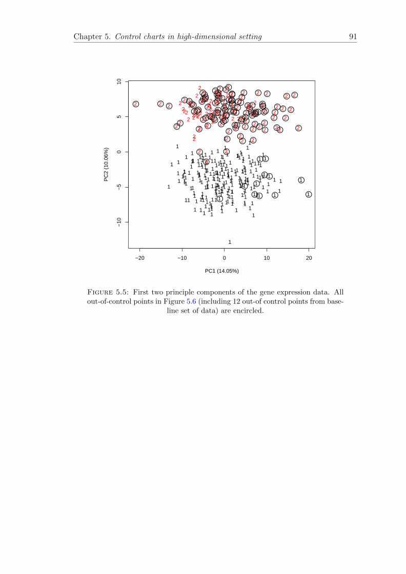
Chapter 5. Control charts in high-dimensional setting 91
−20 −10 0 10 20
−10
−5
05
10
PC1 (14.05%)
PC
2 (1
0.06
%)
1
1
1
11
1
1
1
1
1
11 1
1
1
1
11
1 1
1
11 1
1
11
1 1
11
11
1
1
1
1
1
1
1 1
1
11
1
1
1
11
1
1
1
1
1
1
11
1
1
1 1
11
1
1 1
1
1
1
1
1
1 11
1
1 11
1
1
1
1
1
1
1
1
1
11
1
1
1
1
1
1
1
1
1
1
1
1
1
1 1
1
1
1
1
1
11
1
11
1
1
1
11
1
11
11
1
11
11
1
11
11
11
11
1 1
1
1
1
1
11
1
1
1
11
1
1
1
11
11
11
1
1 1
1
1
11
1
1
1
1
1
1 11
1
1
11
1
1
1
1
1
1
1
1
11
1 1
1
1
1 1
1
1
1
11
1
1
1
1
1
1
11
11
11
1
1
1
1
1
1
1
1
1
1
1
1
1
1
1
1
1
11
1
2
2
2
2 2 2
2
22
2
2
2
2
2
2
2
22
2
2
2
22
22
2
22
22
2
22
22
2
2
2
2
22
2 2
22
22
2
22
22
2
22
22
2
22
2
2
2
2
222
2
2
2
2
22 2
2
2
2
22
2 2
22
22
2
2
2
2
22
2
2
2 22
2
2
22
22
2
2
2
22
22
22 2
2
22
2
2 22
2
2
222
2
2
2
2
2
22
2
2
2 2
2
2
2
2
2
2
2 2
2
222
2
2
2
2
22
2
2 2
22
2
Figure 5.5: First two principle components of the gene expression data. Allout-of-control points in Figure 5.6 (including 12 out-of control points from base-
line set of data) are encircled.

Chapter 5. Control charts in high-dimensional setting 92
050
010
0015
0020
0025
0030
00
1 100 200 300 400
Index
T2
Figure 5.6: Multivariate control chart using study 1 data as a baseline setof data (black) and study 2 as a future set of data (red). The solid line at
T 2 = 853.504 represent the UCL at 5% level of significance.
5.6.2 Example 2: Chemical process data
Here we apply the method to chemical process data with four variables and 30
observations. The data set is given in Table 5.3 and was originally used by Mont-
gomery (2007) to demonstrate the method of principal component analysis for
multivariate process monitoring. Following Montgomery (2007), the first 20 ob-
servations were used as Phase-I data and the last ten observations were used for
testing and monitoring (Phase-II). The scatter plot of the first two principal com-
ponent scores computed using the Phase-I observations is shown in Figure 5.7.
The Phase-II observations are projected onto the PCA plot of Phase-I observa-
tions. The Phase-II observations are represented by a different plotting symbols
together with the numbers from 21 to 30, to show the sequence of points. The
observations outside the 99% confidence ellipse are considered the out-of-control
signals and indicates that there has been a shift in the process mean. We analyze

Chapter 5. Control charts in high-dimensional setting 93
the data using our method and present the control chart in Figure 5.8. It is clear
that our method shows more sensitivity and detects the shift one point in time
earlier than the principal component trajectory plot.
To further assess our method in comparison with the principal components ap-
proach under a smaller sample size, we drop the first 10 observations of the baseline
data and re-analyze the data using the middle 10 observations as a baseline set
of data. The resultant PCA plot shown in Figure 5.9 while the control chart pro-
duced by our method is in Figure 5.10. The PCA performance is poor – because it
fails to identify most of the out-of-control observations as only three observations
(24rd, 26th, and 29th) are outside the 99% confidence ellipse. On the other hand,
our method seems to be robust to the change in the sample size. It has detected
23rd the out-of-control signals even with the smaller Phase-I sample size (n = 10).
−4 −2 0 2 4 6
−6
−4
−2
02
4
PC1 (57.95%)
PC
2 (2
5.30
%)
2122
23
24
25
26
27
28 29
30
**
*
*
**
*
* *
*
Figure 5.7: Principal components trajectory plot for the chemical process datawith 99% confidence ellipse. Only the first 20 baseline observations are used tocompute the principal components. The 10 future observation are plotted withstar symbols and are numbered from 21 to 30 in order to show the natural
sequence of the points.

Chapter 5. Control charts in high-dimensional setting 94
0 5 10 15 20 25 30
020
4060
Index
T2
Figure 5.8: Control chart produced by the proposed method for monitoringthe chemical process data shown in Figure 5.7. The first 20 observations areused to estimate the control limits. The solid line at T 2 = 11.1887 indicates the
control limit of the chart at 1% level of significance.

Chapter 5. Control charts in high-dimensional setting 95
−4 −2 0 2 4 6
−6
−4
−2
02
4
PC1 (66.14%)
PC
2 (2
2.13
%)
21
22
23
24
25
26
27
28
29
30*
*
*
*
*
*
**
*
*
Figure 5.9: Principal components trajectory plot for the chemical processdata with 99% confidence ellipse. Note that the first 10 baseline observations aredropped from the analysis and the principal components are computed from themiddle 10 observations. The last 10 observations are plotted with star symbolsand are numbered from 21 to 30 in order to show the natural sequence of the
points.

Chapter 5. Control charts in high-dimensional setting 96
5 10 15 20
010
2030
4050
60
Index
T2
Figure 5.10: Control chart produced by the proposed method for monitoringthe chemical process data shown in Figure 5.9. Only the middle 10 observationsare used to estimate the empirical reference distribution. The solid line at T 2 =13.1733 indicates the control limit of the chart at at 1% level of significance.
5.7 Summary and Conclusion
In this Chapter, we propose a method to detect unusual observations or changes
in a high-dimensional stochastic process. In high-dimensional problems, the T 2
statistic is impossible to calculate if p > n and even when p < n the standard
theory (Hotelling T 2 control charts) leads to a procedure with low power. We
chose the shrinkage estimation of the covariance matrix to not only make the cal-
culation of T 2 possible, but also reliable. Other regularization techniques for the
covariance matrix (e.g. ridge or lasso regularization) could be used, but they are
computationally expensive, typically relying on cross validation and use normal
likelihood to select the value of the penalty parameter. One reason for choosing
the shrinkage estimate is that it is based on a fully automated and computationally
inexpensive data driven method. Other reason for choosing shrinkage estimator is

Chapter 5. Control charts in high-dimensional setting 97
that it does not make any distributional assumptions about the underlying distri-
bution of the data and its performance advantages are potentially not restricted
to Gaussian assumptions. This was combined with a leave-one-out re-sampling
procedure to obtain n independent T 2 values. To estimate the distribution of T 2
for future observations, we used kernel smoothing. The UCL for monitoring future
observations was the (1− α)th quantile of the kernel smoothed distribution.
The performance of the procedure was evaluated using extensive Monte Carlo
simulation. The method was compared with the standard procedure wherever
possible and also with a hypothetically best case, based on the true parameters. We
showed numerically that the new procedure competes well and had considerable
power to detect signals under various simulations. The ability of the procedure to
accurately characterize the shift in mean vector is also shown by applying it to a
gene expression data, where we use data from two studies with different protocols
to demonstrate detecting a protocol change or error. One natural competitor of
the proposed method is the principal component approach. We use the chemical
process data (previously used to demonstrate the principal component approach)
to show the advantages of the proposed method.
The method may perform well in multivariate non-normal data, as it does not
assume the data to be normally distributed. Further simulation, however, would
be required to investigate the performance of the method in this more general
setting. We leave assessment of this to future work.
The control charts generally use much lower false alarm rates. Our procedure
works well for larger significance values (e.g., 5%). Therefore, this approach will
be useful in situations where there is a high priority of quickly detecting any shift
in the process, or where the follow-up to a detected outlier is easy and inexpensive,
so that a higher false alarm rate can be tolerated. Note also that the proposed
procedure relies on kernel estimation, it is sensitive to the quality and size of the
training sample.
5.8 Contributions of the Chapter
The Hotelling T 2 control chart becomes unreliable and even impractical when
n < p. In this Chapter, we propose a procedure to improve process monitoring in
the high-dimensional setting. We use a shrinkage estimate of the covariance matrix

Chapter 5. Control charts in high-dimensional setting 98
as an estimate of the baseline parameter. A leave-one-out re-sampling procedure
is used to obtain independent T 2 values. The upper control limit for monitoring
the future observations is then calculated from kernel smoothed empirical distri-
bution of the independent T 2 values. The performance of the proposed approach
is tested, and compared to the Hotelling T 2 and the hypothetically “best possi-
ble” results, via an extensive simulation study. The procedure outperforms the
standard Hotelling T 2 method and gives comparable results to the one based on
true parameters. The procedure is also applied to a real gene expression data set
and a chemical process data that has been analyzed in literature to demonstrate
the principal component approach for process monitoring.

Chapter 5. Control charts in high-dimensional setting 99
Table 5.3: Chemical process data. There are total 30 observations. The first20 observations constitute the baseline set of data and the last 10 observations
are the new observations used for testing and monitoring.
Observation x1 x2 x3 x41 10.00 20.70 13.60 15.502 10.50 19.90 18.10 14.803 9.70 20.00 16.10 16.504 9.80 20.20 19.10 17.105 11.70 21.50 19.80 18.306 11.00 20.90 10.30 13.807 8.70 18.80 16.90 16.808 9.50 19.30 15.30 12.209 10.10 19.40 16.20 15.8010 9.50 19.60 13.60 14.5011 10.50 20.30 17.00 16.5012 9.20 19.00 11.50 16.3013 11.30 21.60 14.00 18.7014 10.00 19.80 14.00 15.9015 8.50 19.20 17.40 15.8016 9.70 20.10 10.00 16.6017 8.30 18.40 12.50 14.2018 11.90 21.80 14.10 16.2019 10.30 20.50 15.60 15.1020 8.90 19.00 8.50 14.7021 9.90 20.00 15.40 15.9022 8.70 19.00 9.90 16.8023 11.50 21.80 19.30 12.1024 15.90 24.60 14.70 15.3025 12.60 23.90 17.10 14.2026 14.90 25.00 16.30 16.6027 9.90 23.70 11.90 18.1028 12.80 26.30 13.50 13.7029 13.10 26.10 10.90 16.8030 9.80 25.80 14.80 15.00

Chapter 6
General Conclusions
In recent years, there has been intense activity in improving estimation of the
covariance matrix when n < p, or they are of comparable size. Despite this,
the regularized estimators can be rarely seen in practice. One reason is because
the covariance is merely an ingredient of the common multivariate procedures.
Replacing the sample covariance by its regularized alternatives does not guarantee
that the procedure still works. There is a need to adapt procedures to allow the
use of regularized estimators, and assess these new techniques. When regularized
estimators have found their way into multivariate techniques, their assessment
is frequently restricted to the applications that were the original motivation for
its development. For example, lasso-type regularization has been used primarily
when a sparse covariance is expected, while the shrinkage estimate is common
in portfolio optimization problems. There is a need for a more comprehensive
comparison, to broadly characterize the situations where each method performs
well.
The main objective of this Thesis was to explore some of the important regulariza-
tion techniques for estimation of high-dimensional covariance matrices and their
properties in different high-dimensional multivariate methods. We have investi-
gated the behavior of the regularized alternatives to the sample covariance in three
different multivariate techniques. These are summarized in Sections 6.2, 6.3, and
6.4 with common themes and future directions highlighted in Section 6.5.
100

Chapter 6. General Conclusions 101
6.1 Regularized estimation of the high-dimensional
covariance matrices
The behavior of the sample covariance in high-dimensional problems is well-known
to be poor. In recent years various regularization techniques have been developed
to improve over the sample covariance in a high-dimensional setting. Chapter 2
reviews some of the important recent regularization techniques. These techniques
include the shrinkage estimation of the sample covariance matrix, the ridge regular-
ization, the lasso regularization, and weighted versions of the lasso regularization.
To assess how well different regularized estimators perform to estimate the true co-
variance matrix, a simulation study was conducted. The lasso estimator, although
computationally intensive and assuming multivariate normality, has the compet-
itive accuracy. The shrinkage estimator, on the other hand, is computationally
inexpensive and does not make distributional assumption about the underlying
set of data. The ridge estimator differs from the shrinkage estimator in that it
chooses the shrinkage parameter using cross-validation. In our simulations, we
found no advantage of the cross-validation over the computationally fast closed
form expression used to estimate the shrinkage intensity for the shrinkage esti-
mator. Our simulations show that the covariance matrix can be more accurately
estimated using lasso penalty (if diagonal elements are not penalized) rather than
using adaptive lasso and SCAD penalties that are shown to be superior to the
lasso penalty in model selection.
6.2 Hierarchical covariance estimation
Multivariate random effect models need proper estimates of the within-group and
the between-group covariance matrices. The computation of a between-group co-
variance involves the difference of two mean-square matrices and often results nega-
tive elements on the diagonal. The probability of negative elements increases as we
increase the number of variables. This makes it difficult, in the high-dimensional
setting, to obtain a proper between-group covariance matrix. In Chapter 3, a hi-
erarchical model is proposed based on the EM-algorithm. The Lasso-regularized
estimates of the covariance matrices are embedded in the algorithm to ensure es-
timates of covariance matrices are positive definite. Our simulation study showed

Chapter 6. General Conclusions 102
that the proposed model performs well and returns a positive definite estimate of
the between-group covariance. We applied the method to a glass chemical compo-
sition data. In this data set, we are interested in the between-group covariance and
the standard estimate is not positive definite. We show that using the proposed
method one can obtain a proper between-group covariance. In our simulation
experiments, the algorithm needed few iterations to converge (especially in cases
where the between-group variation is dominant) and is a good replacement in the
situations where the traditional analysis of variance technique fails to work.
6.3 Regularized MANOVA for high-dimensional
data
MANOVA is used to test hypothesis of group effects on multiple response variables
simultaneously. High-dimensionality poses a serious problem to MANOVA tests.
We have shown that the estimation error in terms of eigenvalues of covariance
matrices is the least, on average, for the lasso-regularized covariance matrix in
comparison with ridge and shrinkage estimates. In Chapter 4 of the Thesis, we
propose an approach based on the lasso regularization. We investigate the behav-
ior of the novel approach via extensive simulations taking into account a number
of different factors. The new approach is also compared with other existing ap-
proaches.
In our simulation experiments, the three recent high-dimensional regularization
procedures of the sample covariance: the shrinkage, the ridge, and the lasso regu-
larization perform well, and in many cases perform better than the more conven-
tional generalized inverse and principal component approach. None of the shrink-
age, the ridge, and lasso is universally superior across scenarios considered in our
simulation study. Lasso regularization is always the best when the shift is along
all the eigenvectors but the difference is not dramatic. The difference, however,
increases as we increase the number of variables. The better performance of lasso
regularization seems to be because of its better recovery of the true eigenvalues.
Lasso regularization, however, is computationally expensive than the other com-
peting procedures we have considered in this study. This is because lasso regular-
ization by itself is an iterative procedure. The two computationally cumbersome

Chapter 6. General Conclusions 103
jobs, cross-validation to choose penalty parameter and permutation test, add sub-
stantially to its computational time. While not computationally prohibitive its
computational time is increasing dramatically with the number of variables for a
fixed sample size. Ridge regularization is comparatively less expensive than lasso
but its implementation also involves cross-validation. Principal component ap-
proach, generalize inverse and shrinkage approach are computationally simple and
very fast. However, the performance of principal component approach have been
very poor both in our simulation experiments and the real data. The performance
of generalized inverse has been very poor in the zone where p is large but close to
n. Taking both things — power and computational time— into consideration the
shrinkage approach has an excellent balance.
6.4 Monitoring individual future observations in
the high-dimensional setup
The Hotelling T 2 control chart is used to detect unusual changes in the mean
vector of a stochastic process while monitoring individual future observations. In
high-dimensional problems the T 2 statistic is impossible to calculate if n < p and
even for n > p, the UCL of the Hotelling T 2 control chart for monitoring future
observations is unknown. In Chapter 5, a new method is proposed for monitoring
future observations in high-dimensional setting. The method is superior to the
standard Hotelling T 2 control chart in practice.
We evaluate the performance of the novel procedure using extensive Monte Carlo
simulation. The method is also compared with the standard procedure wherever
possible and also with a hypothetical “best case” that is based on the true pa-
rameters. We show numerically that the new procedure competes well and gains
considerable power to detect signals under various simulations. The ability of
the procedure to accurately characterize the shift in mean vector is also shown
by applying it to a gene expression data, where we use data from two studies
with different protocols to demonstrate detecting a protocol change or error. One
natural competitor of the proposed method is the principal component approach.
We use the chemical process data (previously used to demonstrate the principal
component approach) to show the out-performance of the proposed method.

Chapter 6. General Conclusions 104
It is important to note that we do not make any particular assumption about
the distribution of the data. The method may perform well in multivariate non-
normal data. Further simulation, however, would be required to investigate the
performance of the method in multivariate non-normal data. Although the new
method is proposed to monitor future observations, it can be used for Phase-I
analysis as well.
6.5 Commonalities and future work
Lasso regularization is being used for identifying zero elements in the inverse co-
variance matrix (model selection in the context of Gaussian graphical models). It
can be used to obtain a regularized estimate of a covariance matrix. The shrinkage
and ridge regularization are being used to estimate high-dimensional covariance
matrices but always produce dense estimate of the inverse covariance matrix. In
Chapter 2 and Chapter 4, the lasso regularization was expected to have a bigger
advantage on the AR(1) structure (because its inverse is sparse) as compared to
the exchangeable structure but it is not true in our simulation. The performance
of the regularized covariance matrix obtained using lasso regularization is better
even if the inverse covariance matrix is not sparse. The computational time of
lasso regularization is, however, less for the covariance structure whose inverse is
sparse.
Chapter 4 and 5 both involve creating reference distributions. In Chapter 5,
we drop one observation from the baseline set of data at a time and estimate
the parameters from the rest. The Hotelling T 2 statistic is calculated for the
observation that was dropped. This gives us only n different T 2 values. The
empirical distribution of the T 2 values is more of a discrete nature (we avoid this
using kernel density estimate) and is not suitable for estimating the p-value. This
is totally different from the permutation test we have used in Chapter 5 because
there are many possible permutations even for a small sample size that produce
many values of the test statistic. The empirical distribution in this case is smoother
and is suitable to estimate p-value.
The first problem that needs to be further investigated is related to the two dimen-
sionality reduction techniques we have considered in Chapter 4, namely, Moore-
Penrose generalized inverse and principal component approach. The generalized

Chapter 6. General Conclusions 105
inverse exhibit rather surprisingly good behavior outside the critical zone (when
n is just less than p) relative to other methods we have considered in Chapter 4.
On the other hand, the performance of the approach based on principal compo-
nents has been poor. Both these methods reduces the dimension of the data. The
generalized inverse reduces the dimension from p to the rank(Σ). It reduces to
standard matrix inverse when rank(Σ) ≥ p. The performance of the standard
inverse covariance matrix is already known to be poor in high-dimensional prob-
lems. The principle component approach reduces the dimension of the data to
first q principal components (q is the number of principal components chosen us-
ing the eigenvalue-greater-than-one rule). The two methods becomes similar and
are expected to provide similar results when the rank(Σ) = q. The performance
of generalized inverse might improve in the critical zone if we use it with fewer
dimensions than the rank(Σ) and do not allow it to reduce to the standard matrix
inverse. A different criteria to choose an intermediate number of dimensions would
be required rather than the rank(Σ) or eigenvalue-greater-than-one rule.
Another problem that needs to be investigated is related to the method we pre-
sented in Chapter 5 for monitoring future observations. To obtain the UCL, a
kernel density approach is used that is good to estimate central quantiles. Another
possibility is to estimate the quantiles using extreme value distribution (Beirlant
et al., 2006). This approach is preferred to estimate the extreme quantiles and
may perform better than the kernel density approach. It needs to be explored.
Finally, real data is frequently non-normal. The Hotelling T 2 control chart method
for detecting unusual future observations assume that the observations follow a
multivariate normal distribution. In the procedure presented in Chapter 5, our
reference distribution is based on an empirically generated distribution, it is valid
even if the data are not normal. The shrinkage approach is also distribution free. It
seems a promising non-parametric alternative and might work well for non-normal
data. Further investigation would be required to study the procedure for different
flavors of non-normality.

Appendix A
Supplementary Figure for
Chapter 4
Table A.1: Values of the shift parameter, δ, used in the simulationexperiments whose results are presented in Figure A.1 and Figure A.2.
Orientation
of δ
Covariance structure
AR(1) Exchangeable
along 1st eigenvector 4.080 5.040
along 2nd eigenvector 2.280 2.280
along pth eigenvector 1.560 1.560
along all eigenvectors 0.516 0.504
106

Appendix A. Supplementary Figure for Chapter 4 107
5 10 15 20 25 30
0.0
0.2
0.4
0.6
0.8
1.0
p
pow
er
PCShrinkageLASSORidgeG.inverse
Shift along 1st eigenvector
5 10 15 20 25 30
0.0
0.2
0.4
0.6
0.8
1.0
p
pow
er
PCShrinkageLASSORidgeG.inverse
Shift along 2nd eigenvector
5 10 15 20 25 30
0.0
0.2
0.4
0.6
0.8
1.0
p
pow
er
PCShrinkageLASSORidgeG.inverse
Shift along pth eigenvector
5 10 15 20 25 30
0.0
0.2
0.4
0.6
0.8
1.0
p
pow
er
PCShrinkageLASSORidgeG.inverse
Shift along all eigenvectors
Figure A.1: Power comparison of MANOVA test based on 5 competing pro-cedures under AR(1) covariance structure with b = 0.4. For each value ofp ∈ [2, 30], the power is estimated using 1000 samples and the significance level
is kept as 0.05.

Appendix A. Supplementary Figure for Chapter 4 108
5 10 15 20 25 30
0.0
0.2
0.4
0.6
0.8
1.0
p
pow
er
PCShrinkageLASSORidgeG.inverse
Shift along 1st eigenvector
5 10 15 20 25 30
0.0
0.2
0.4
0.6
0.8
1.0
p
pow
er
PCShrinkageLASSORidgeG.inverse
Shift along 2nd eigenvector
5 10 15 20 25 30
0.0
0.2
0.4
0.6
0.8
1.0
p
pow
er
PCShrinkageLASSORidgeG.inverse
Shift along pth eigenvector
5 10 15 20 25 30
0.0
0.2
0.4
0.6
0.8
1.0
p
pow
er
PCShrinkageLASSORidgeG.inverse
Shift along all eigenvectors
Figure A.2: Power comparison of MANOVA test based on 5 competing pro-cedures under exchangeable covariance structure with b = 0.4. For each valueof p ∈ [2, 30], the power is estimated using 1000 samples and the significance
level is kept as 0.05.

Appendix B
Supplementary Figure for
Chapter 5
109

Appendix B. Supplementary Figures for Chapter 5 110
0 10 20 30 40 50 60
0.0
0.2
0.4
0.6
0.8
1.0
p
Fals
e al
arm
rat
e
Pow
erShift along all eigenvectors
α = 0.1
0 10 20 30 40 50 60
0.0
0.2
0.4
0.6
0.8
1.0
p
Fals
e al
arm
rat
e
Pow
er
Shift along all eigenvectors
α = 0.05
0 10 20 30 40 50 60
0.0
0.2
0.4
0.6
0.8
1.0
p
Fals
e al
arm
rat
e
Pow
er
Shift along all eigenvectors
α = 0.01
0 10 20 30 40 50 60
0.0
0.2
0.4
0.6
0.8
1.0
p
Fals
e al
arm
rat
e
Pow
er
Shift along 1st eigenvector
α = 0.1
0 10 20 30 40 50 60
0.0
0.2
0.4
0.6
0.8
1.0
p
Fals
e al
arm
rat
e
Pow
er
Shift along 1st eigenvector
α = 0.05
0 10 20 30 40 50 60
0.0
0.2
0.4
0.6
0.8
1.0
pFa
lse
alar
m r
ate
P
ower
Shift along 1st eigenvector
α = 0.01
0 10 20 30 40 50 60
0.0
0.2
0.4
0.6
0.8
1.0
p
Fals
e al
arm
rat
e
Pow
er
Shift along 2nd eigenvector
α = 0.1
0 10 20 30 40 50 60
0.0
0.2
0.4
0.6
0.8
1.0
p
Fals
e al
arm
rat
e
Pow
er
Shift along 2nd eigenvector
α = 0.05
0 10 20 30 40 50 60
0.0
0.2
0.4
0.6
0.8
1.0
p
Fals
e al
arm
rat
e
Pow
er
Shift along 2nd eigenvector
α = 0.01
0 10 20 30 40 50 60
0.0
0.2
0.4
0.6
0.8
1.0
p
Fals
e al
arm
rat
e
Pow
er
Shift along pth eigenvector
α = 0.1
0 10 20 30 40 50 60
0.0
0.2
0.4
0.6
0.8
1.0
p
Fals
e al
arm
rat
e
Pow
er
Shift along pth eigenvector
α = 0.05
0 10 20 30 40 50 60
0.0
0.2
0.4
0.6
0.8
1.0
p
Fals
e al
arm
rat
e
Pow
er
Shift along pth eigenvector
α = 0.01
Figure B.1: Power (solid lines) and false alarm rate (dashed lines) for AR(1)covariance structure with b = 0.3. The black lines are based on the true param-eters and therefore are the best possible results one can achieve. The green linesare the results for standard method (using sample mean and sample covariance
matrix) and the blue lines are the results from new method.

Appendix B. Supplementary Figures for Chapter 5 111
0 10 20 30 40 50 60
0.0
0.2
0.4
0.6
0.8
1.0
p
Fals
e al
arm
rat
e
Pow
erShift along all eigenvectors
α = 0.1
0 10 20 30 40 50 60
0.0
0.2
0.4
0.6
0.8
1.0
p
Fals
e al
arm
rat
e
Pow
er
Shift along all eigenvectors
α = 0.05
0 10 20 30 40 50 60
0.0
0.2
0.4
0.6
0.8
1.0
p
Fals
e al
arm
rat
e
Pow
er
Shift along all eigenvectors
α = 0.01
0 10 20 30 40 50 60
0.0
0.2
0.4
0.6
0.8
1.0
p
Fals
e al
arm
rat
e
Pow
er
Shift along 1st eigenvector
α = 0.1
0 10 20 30 40 50 60
0.0
0.2
0.4
0.6
0.8
1.0
p
Fals
e al
arm
rat
e
Pow
er
Shift along 1st eigenvector
α = 0.05
0 10 20 30 40 50 60
0.0
0.2
0.4
0.6
0.8
1.0
pFa
lse
alar
m r
ate
P
ower
Shift along 1st eigenvector
α = 0.01
0 10 20 30 40 50 60
0.0
0.2
0.4
0.6
0.8
1.0
p
Fals
e al
arm
rat
e
Pow
er
Shift along 2nd eigenvector
α = 0.1
0 10 20 30 40 50 60
0.0
0.2
0.4
0.6
0.8
1.0
p
Fals
e al
arm
rat
e
Pow
er
Shift along 2nd eigenvector
α = 0.05
0 10 20 30 40 50 60
0.0
0.2
0.4
0.6
0.8
1.0
p
Fals
e al
arm
rat
e
Pow
er
Shift along 2nd eigenvector
α = 0.01
0 10 20 30 40 50 60
0.0
0.2
0.4
0.6
0.8
1.0
p
Fals
e al
arm
rat
e
Pow
er
Shift along pth eigenvector
α = 0.1
0 10 20 30 40 50 60
0.0
0.2
0.4
0.6
0.8
1.0
p
Fals
e al
arm
rat
e
Pow
er
Shift along pth eigenvector
α = 0.05
0 10 20 30 40 50 60
0.0
0.2
0.4
0.6
0.8
1.0
p
Fals
e al
arm
rat
e
Pow
er
Shift along pth eigenvector
α = 0.01
Figure B.2: Power (solid lines) and false alarm rate (dashed lines) for AR(1)covariance structure with b = 0.4. The black lines are based on the true param-eters and therefore are the best possible results one can achieve. The green linesare the results for standard method (using sample mean and sample covariance
matrix) and the blue lines are the results from new method.

Appendix B. Supplementary Figures for Chapter 5 112
0 10 20 30 40 50 60
0.0
0.2
0.4
0.6
0.8
1.0
p
Fals
e al
arm
rat
e
Pow
erShift along all eigenvectors
α = 0.1
0 10 20 30 40 50 60
0.0
0.2
0.4
0.6
0.8
1.0
p
Fals
e al
arm
rat
e
Pow
er
Shift along all eigenvectors
α = 0.05
0 10 20 30 40 50 60
0.0
0.2
0.4
0.6
0.8
1.0
p
Fals
e al
arm
rat
e
Pow
er
Shift along all eigenvectors
α = 0.01
0 10 20 30 40 50 60
0.0
0.2
0.4
0.6
0.8
1.0
p
Fals
e al
arm
rat
e
Pow
er
Shift along 1st eigenvector
α = 0.1
0 10 20 30 40 50 60
0.0
0.2
0.4
0.6
0.8
1.0
p
Fals
e al
arm
rat
e
Pow
er
Shift along 1st eigenvector
α = 0.05
0 10 20 30 40 50 60
0.0
0.2
0.4
0.6
0.8
1.0
pFa
lse
alar
m r
ate
P
ower
Shift along 1st eigenvector
α = 0.01
0 10 20 30 40 50 60
0.0
0.2
0.4
0.6
0.8
1.0
p
Fals
e al
arm
rat
e
Pow
er
Shift along 2nd eigenvector
α = 0.1
0 10 20 30 40 50 60
0.0
0.2
0.4
0.6
0.8
1.0
p
Fals
e al
arm
rat
e
Pow
er
Shift along 2nd eigenvector
α = 0.05
0 10 20 30 40 50 60
0.0
0.2
0.4
0.6
0.8
1.0
p
Fals
e al
arm
rat
e
Pow
er
Shift along 2nd eigenvector
α = 0.01
0 10 20 30 40 50 60
0.0
0.2
0.4
0.6
0.8
1.0
p
Fals
e al
arm
rat
e
Pow
er
Shift along pth eigenvector
α = 0.1
0 10 20 30 40 50 60
0.0
0.2
0.4
0.6
0.8
1.0
p
Fals
e al
arm
rat
e
Pow
er
Shift along pth eigenvector
α = 0.05
0 10 20 30 40 50 60
0.0
0.2
0.4
0.6
0.8
1.0
p
Fals
e al
arm
rat
e
Pow
er
Shift along pth eigenvector
α = 0.01
Figure B.3: Power (solid lines) and false alarm rate (dashed lines) for AR(1)covariance structure with b = 0.6. The black lines are based on the true param-eters and therefore are the best possible results one can achieve. The green linesare the results for standard method (using sample mean and sample covariance
matrix) and the blue lines are the results from new method.

Appendix B. Supplementary Figures for Chapter 5 113
0 10 20 30 40 50 60
0.0
0.2
0.4
0.6
0.8
1.0
p
Fals
e al
arm
rat
e
Pow
erShift along all eigenvectors
α = 0.1
0 10 20 30 40 50 60
0.0
0.2
0.4
0.6
0.8
1.0
p
Fals
e al
arm
rat
e
Pow
er
Shift along all eigenvectors
α = 0.05
0 10 20 30 40 50 60
0.0
0.2
0.4
0.6
0.8
1.0
p
Fals
e al
arm
rat
e
Pow
er
Shift along all eigenvectors
α = 0.01
0 10 20 30 40 50 60
0.0
0.2
0.4
0.6
0.8
1.0
p
Fals
e al
arm
rat
e
Pow
er
Shift along 1st eigenvector
α = 0.1
0 10 20 30 40 50 60
0.0
0.2
0.4
0.6
0.8
1.0
p
Fals
e al
arm
rat
e
Pow
er
Shift along 1st eigenvector
α = 0.05
0 10 20 30 40 50 60
0.0
0.2
0.4
0.6
0.8
1.0
pFa
lse
alar
m r
ate
P
ower
Shift along 1st eigenvector
α = 0.01
0 10 20 30 40 50 60
0.0
0.2
0.4
0.6
0.8
1.0
p
Fals
e al
arm
rat
e
Pow
er
Shift along 2nd eigenvector
α = 0.1
0 10 20 30 40 50 60
0.0
0.2
0.4
0.6
0.8
1.0
p
Fals
e al
arm
rat
e
Pow
er
Shift along 2nd eigenvector
α = 0.05
0 10 20 30 40 50 60
0.0
0.2
0.4
0.6
0.8
1.0
p
Fals
e al
arm
rat
e
Pow
er
Shift along 2nd eigenvector
α = 0.01
0 10 20 30 40 50 60
0.0
0.2
0.4
0.6
0.8
1.0
p
Fals
e al
arm
rat
e
Pow
er
Shift along pth eigenvector
α = 0.1
0 10 20 30 40 50 60
0.0
0.2
0.4
0.6
0.8
1.0
p
Fals
e al
arm
rat
e
Pow
er
Shift along pth eigenvector
α = 0.05
0 10 20 30 40 50 60
0.0
0.2
0.4
0.6
0.8
1.0
p
Fals
e al
arm
rat
e
Pow
er
Shift along pth eigenvector
α = 0.01
Figure B.4: Power (solid lines) and false alarm rate (dashed lines) for AR(1)covariance structure with b = 0.7. The black lines are based on the true param-eters and therefore are the best possible results one can achieve. The green linesare the results for standard method (using sample mean and sample covariance
matrix) and the blue lines are the results from new method.

Appendix B. Supplementary Figures for Chapter 5 114
0 10 20 30 40 50 60
0.0
0.2
0.4
0.6
0.8
1.0
p
Fals
e al
arm
rat
e
Pow
erShift along all eigenvectors
α = 0.1
0 10 20 30 40 50 60
0.0
0.2
0.4
0.6
0.8
1.0
p
Fals
e al
arm
rat
e
Pow
er
Shift along all eigenvectors
α = 0.05
0 10 20 30 40 50 60
0.0
0.2
0.4
0.6
0.8
1.0
p
Fals
e al
arm
rat
e
Pow
er
Shift along all eigenvectors
α = 0.01
0 10 20 30 40 50 60
0.0
0.2
0.4
0.6
0.8
1.0
p
Fals
e al
arm
rat
e
Pow
er
Shift along 1st eigenvector
α = 0.1
0 10 20 30 40 50 60
0.0
0.2
0.4
0.6
0.8
1.0
p
Fals
e al
arm
rat
e
Pow
er
Shift along 1st eigenvector
α = 0.05
0 10 20 30 40 50 60
0.0
0.2
0.4
0.6
0.8
1.0
pFa
lse
alar
m r
ate
P
ower
Shift along 1st eigenvector
α = 0.01
0 10 20 30 40 50 60
0.0
0.2
0.4
0.6
0.8
1.0
p
Fals
e al
arm
rat
e
Pow
er
Shift along 2nd eigenvector
α = 0.1
0 10 20 30 40 50 60
0.0
0.2
0.4
0.6
0.8
1.0
p
Fals
e al
arm
rat
e
Pow
er
Shift along 2nd eigenvector
α = 0.05
0 10 20 30 40 50 60
0.0
0.2
0.4
0.6
0.8
1.0
p
Fals
e al
arm
rat
e
Pow
er
Shift along 2nd eigenvector
α = 0.01
0 10 20 30 40 50 60
0.0
0.2
0.4
0.6
0.8
1.0
p
Fals
e al
arm
rat
e
Pow
er
Shift along pth eigenvector
α = 0.1
0 10 20 30 40 50 60
0.0
0.2
0.4
0.6
0.8
1.0
p
Fals
e al
arm
rat
e
Pow
er
Shift along pth eigenvector
α = 0.05
0 10 20 30 40 50 60
0.0
0.2
0.4
0.6
0.8
1.0
p
Fals
e al
arm
rat
e
Pow
er
Shift along pth eigenvector
α = 0.01
Figure B.5: Power (solid lines) and false alarm rate (dashed lines) for ex-changeable covariance structure with b = 0.3. The black lines are based on thetrue parameters and therefore are the best possible results one can achieve. Thegreen lines are the results for standard method (using sample mean and sample
covariance matrix) and the blue lines are the results from new method.

Appendix B. Supplementary Figures for Chapter 5 115
0 10 20 30 40 50 60
0.0
0.2
0.4
0.6
0.8
1.0
p
Fals
e al
arm
rat
e
Pow
erShift along all eigenvectors
α = 0.1
0 10 20 30 40 50 60
0.0
0.2
0.4
0.6
0.8
1.0
p
Fals
e al
arm
rat
e
Pow
er
Shift along all eigenvectors
α = 0.05
0 10 20 30 40 50 60
0.0
0.2
0.4
0.6
0.8
1.0
p
Fals
e al
arm
rat
e
Pow
er
Shift along all eigenvectors
α = 0.01
0 10 20 30 40 50 60
0.0
0.2
0.4
0.6
0.8
1.0
p
Fals
e al
arm
rat
e
Pow
er
Shift along 1st eigenvector
α = 0.1
0 10 20 30 40 50 60
0.0
0.2
0.4
0.6
0.8
1.0
p
Fals
e al
arm
rat
e
Pow
er
Shift along 1st eigenvector
α = 0.05
0 10 20 30 40 50 60
0.0
0.2
0.4
0.6
0.8
1.0
pFa
lse
alar
m r
ate
P
ower
Shift along 1st eigenvector
α = 0.01
0 10 20 30 40 50 60
0.0
0.2
0.4
0.6
0.8
1.0
p
Fals
e al
arm
rat
e
Pow
er
Shift along 2nd eigenvector
α = 0.1
0 10 20 30 40 50 60
0.0
0.2
0.4
0.6
0.8
1.0
p
Fals
e al
arm
rat
e
Pow
er
Shift along 2nd eigenvector
α = 0.05
0 10 20 30 40 50 60
0.0
0.2
0.4
0.6
0.8
1.0
p
Fals
e al
arm
rat
e
Pow
er
Shift along 2nd eigenvector
α = 0.01
0 10 20 30 40 50 60
0.0
0.2
0.4
0.6
0.8
1.0
p
Fals
e al
arm
rat
e
Pow
er
Shift along pth eigenvector
α = 0.1
0 10 20 30 40 50 60
0.0
0.2
0.4
0.6
0.8
1.0
p
Fals
e al
arm
rat
e
Pow
er
Shift along pth eigenvector
α = 0.05
0 10 20 30 40 50 60
0.0
0.2
0.4
0.6
0.8
1.0
p
Fals
e al
arm
rat
e
Pow
er
Shift along pth eigenvector
α = 0.01
Figure B.6: Power (solid lines) and false alarm rate (dashed lines) for ex-changeable covariance structure with b = 0.4. The black lines are based on thetrue parameters and therefore are the best possible results one can achieve. Thegreen lines are the results for standard method (using sample mean and sample
covariance matrix) and the blue lines are the results from new method.

Appendix B. Supplementary Figures for Chapter 5 116
0 10 20 30 40 50 60
0.0
0.2
0.4
0.6
0.8
1.0
p
Fals
e al
arm
rat
e
Pow
erShift along all eigenvectors
α = 0.1
0 10 20 30 40 50 60
0.0
0.2
0.4
0.6
0.8
1.0
p
Fals
e al
arm
rat
e
Pow
er
Shift along all eigenvectors
α = 0.05
0 10 20 30 40 50 60
0.0
0.2
0.4
0.6
0.8
1.0
p
Fals
e al
arm
rat
e
Pow
er
Shift along all eigenvectors
α = 0.01
0 10 20 30 40 50 60
0.0
0.2
0.4
0.6
0.8
1.0
p
Fals
e al
arm
rat
e
Pow
er
Shift along 1st eigenvector
α = 0.1
0 10 20 30 40 50 60
0.0
0.2
0.4
0.6
0.8
1.0
p
Fals
e al
arm
rat
e
Pow
er
Shift along 1st eigenvector
α = 0.05
0 10 20 30 40 50 60
0.0
0.2
0.4
0.6
0.8
1.0
pFa
lse
alar
m r
ate
P
ower
Shift along 1st eigenvector
α = 0.01
0 10 20 30 40 50 60
0.0
0.2
0.4
0.6
0.8
1.0
p
Fals
e al
arm
rat
e
Pow
er
Shift along 2nd eigenvector
α = 0.1
0 10 20 30 40 50 60
0.0
0.2
0.4
0.6
0.8
1.0
p
Fals
e al
arm
rat
e
Pow
er
Shift along 2nd eigenvector
α = 0.05
0 10 20 30 40 50 60
0.0
0.2
0.4
0.6
0.8
1.0
p
Fals
e al
arm
rat
e
Pow
er
Shift along 2nd eigenvector
α = 0.01
0 10 20 30 40 50 60
0.0
0.2
0.4
0.6
0.8
1.0
p
Fals
e al
arm
rat
e
Pow
er
Shift along pth eigenvector
α = 0.1
0 10 20 30 40 50 60
0.0
0.2
0.4
0.6
0.8
1.0
p
Fals
e al
arm
rat
e
Pow
er
Shift along pth eigenvector
α = 0.05
0 10 20 30 40 50 60
0.0
0.2
0.4
0.6
0.8
1.0
p
Fals
e al
arm
rat
e
Pow
er
Shift along pth eigenvector
α = 0.01
Figure B.7: Power (solid lines) and false alarm rate (dashed lines) for ex-changeable covariance structure with b = 0.6. The black lines are based on thetrue parameters and therefore are the best possible results one can achieve. Thegreen lines are the results for standard method (using sample mean and sample
covariance matrix) and the blue lines are the results from new method.

Appendix B. Supplementary Figures for Chapter 5 117
0 10 20 30 40 50 60
0.0
0.2
0.4
0.6
0.8
1.0
p
Fals
e al
arm
rat
e
Pow
erShift along all eigenvectors
α = 0.1
0 10 20 30 40 50 60
0.0
0.2
0.4
0.6
0.8
1.0
p
Fals
e al
arm
rat
e
Pow
er
Shift along all eigenvectors
α = 0.05
0 10 20 30 40 50 60
0.0
0.2
0.4
0.6
0.8
1.0
p
Fals
e al
arm
rat
e
Pow
er
Shift along all eigenvectors
α = 0.01
0 10 20 30 40 50 60
0.0
0.2
0.4
0.6
0.8
1.0
p
Fals
e al
arm
rat
e
Pow
er
Shift along 1st eigenvector
α = 0.1
0 10 20 30 40 50 60
0.0
0.2
0.4
0.6
0.8
1.0
p
Fals
e al
arm
rat
e
Pow
er
Shift along 1st eigenvector
α = 0.05
0 10 20 30 40 50 60
0.0
0.2
0.4
0.6
0.8
1.0
pFa
lse
alar
m r
ate
P
ower
Shift along 1st eigenvector
α = 0.01
0 10 20 30 40 50 60
0.0
0.2
0.4
0.6
0.8
1.0
p
Fals
e al
arm
rat
e
Pow
er
Shift along 2nd eigenvector
α = 0.1
0 10 20 30 40 50 60
0.0
0.2
0.4
0.6
0.8
1.0
p
Fals
e al
arm
rat
e
Pow
er
Shift along 2nd eigenvector
α = 0.05
0 10 20 30 40 50 60
0.0
0.2
0.4
0.6
0.8
1.0
p
Fals
e al
arm
rat
e
Pow
er
Shift along 2nd eigenvector
α = 0.01
0 10 20 30 40 50 60
0.0
0.2
0.4
0.6
0.8
1.0
p
Fals
e al
arm
rat
e
Pow
er
Shift along pth eigenvector
α = 0.1
0 10 20 30 40 50 60
0.0
0.2
0.4
0.6
0.8
1.0
p
Fals
e al
arm
rat
e
Pow
er
Shift along pth eigenvector
α = 0.05
0 10 20 30 40 50 60
0.0
0.2
0.4
0.6
0.8
1.0
p
Fals
e al
arm
rat
e
Pow
er
Shift along pth eigenvector
α = 0.01
Figure B.8: Power (solid lines) and false alarm rate (dashed lines) for ex-changeable covariance structure with b = 0.7. The black lines are based on thetrue parameters and therefore are the best possible results one can achieve. Thegreen lines are the results for standard method (using sample mean and sample
covariance matrix) and the blue lines are the results from new method.

Appendix C
DRC forms
The signed statement of contribution to doctoral thesis containing publications is
attached immediately followed this page.
118

References
Aitken, C. G., & Lucy, D. (2004). Evaluation of trace evidence in the form of
multivariate data. Journal of the Royal Statistical Society: Series C (Applied
Statistics), 53 (1), 109–122.
Amemiya, Y. (1985). What should be done when an estimated between-group
covariance matrix is not nonnegative definite? The American Statistician,
39 (2), 112–117.
Anderson, T. W. (2003). An introduction to multivariate statistical analysis. Wiley
New York.
Beirlant, J., Goegebeur, Y., Segers, J., & Teugels, J. (2006). Statistics of extremes:
theory and applications. John Wiley & Sons.
Bennett, R. L. (2002). Aspects of the analysis and interpretation of glass trace
evidence. Unpublished master’s thesis, New Zealand.
Bersimis, S., Psarakis, S., & Panaretos, J. (2007). Multivariate statistical process
control charts: an overview. Quality and Reliability Engineering International ,
23 (5), 517–543.
Bickel, J., & Levina, E. (2007). Covariance regularization by thresholding (Tech.
Rep.).
Calvin, J. A. (1993). Reml estimation in unbalanced multivariate variance com-
ponents models using an em algorithm. Biometrics , 691–701.
Calvin, J. A., & Dykstra, R. L. (1991). Maximum likelihood estimation of a
set of covariance matrices under lowner order restrictions with applications to
balanced multivariate variance components models. The Annals of Statistics ,
850–869.
119

Bibliography 120
Champ, C. W., Jones-Farmer, L. A., & Rigdon, S. E. (2005). Properties of the
T 2 control chart when parameters are estimated. Technometrics , 47 (4).
Chou, Y., Mason, R. L., & Young, J. C. (1999). Power comparisons for a
Hotelling’s T 2 statistic. Communications in Statistics - Simulation and Com-
putation, 28 (4), 1031-1050.
Cox, D. R., & Wermuth, N. (1996). Multivariate dependencies: Models, analysis
and interpretation (Vol. 67). CRC Press.
Dempster, A. P. (1972). Covariance selection. Biometrics , 28 (1), pp. 157-175.
Dempster, A. P., Laird, N. M., & Rubin, D. B. (1977). Maximum likelihood from
incomplete data via the em algorithm. Journal of the Royal Statistical Society.
Series B (Methodological), 1–38.
Dey, D. K., & Srinivasan, C. (1985). Estimation of a covariance matrix under
stein’s loss. The Annals of Statistics , 1581–1591.
Duong, T. (2014). ks: Kernel smoothing [Computer software manual]. Available
from http://CRAN.R-project.org/package=ks (R package version 1.9.2)
Edgington, E., & Onghena, P. (2007). Randomization tests. CRC Press.
Fan, J., Feng, Y., & Wu, Y. (2009). Network exploration via the adaptive lasso
and scad penalties. The Annals of Applied Statistics , 3 (2), 521.
Fan, J., & Li, R. (2001). Variable selection via nonconcave penalized likelihood and
its oracle properties. Journal of the American Statistical Association, 96 (456),
1348–1360.
Fan, J., Peng, H., et al. (2004). Nonconcave penalized likelihood with a diverging
number of parameters. The Annals of Statistics , 32 (3), 928–961.
Fitch, A. M., Jones, M. B., & Massam, H. (2014). The performance of covariance
selection methods that consider decomposable models only. Bayesian Analysis ,
9 (3), 659–684.
Friedman, J., Hastie, T., Hofling, H., Tibshirani, R., et al. (2007). Pathwise
coordinate optimization. The Annals of Applied Statistics , 1 (2), 302–332.
Friedman, J., Hastie, T., & Tibshirani, R. (2008). Sparse inverse covariance
estimation with the graphical lasso. Biostatistics , 9 (3), 432–441.

Bibliography 121
Friedman, J., Hastie, T., & Tibshirani, R. (2013). glasso: Graphical lasso- estima-
tion of gaussian graphical models [Computer software manual]. Available from
http://www-stat.stanford.edu/~tibs/glasso (R package version 1.7)
Gao, X., Pu, D. Q., Wu, Y., & Xu, H. (2009). Tuning parameter selection for
penalized likelihood estimation of inverse covariance matrix. ArXiv e-prints .
Golub, G., & Kahan, W. (1965). Calculating the singular values and pseudo-
inverse of a matrix. Journal of the Society for Industrial & Applied Mathematics,
Series B: Numerical Analysis , 2 (2), 205–224.
Haff, L. (1980). Empirical Bayes estimation of the multivariate normal covariance
matrix. The Annals of Statistics , 586–597.
Harville, D. A. (1977). Maximum likelihood approaches to variance component
estimation and to related problems. Journal of the American Statistical Asso-
ciation, 72 (358), 320–338.
Hastie, T., Tibshirani, R., Friedman, J., Hastie, T., Friedman, J., & Tibshirani,
R. (2009). The elements of statistical learning (Vol. 2) (No. 1). Springer.
Hill, W. G., & Thompson, R. (1978). Probabilities of non-positive definite
between-group or genetic covariance matrices. Biometrics , 34 (3), pp. 429-439.
Available from http://www.jstor.org/stable/2530605
Huang, J. Z., Liu, N., Pourahmadi, M., & Liu, L. (2006). Covariance matrix
selection and estimation via penalised normal likelihood. Biometrika, 93 (1),
85-98. Available from http://biomet.oxfordjournals.org/content/93/1/
85.abstract
James, W., & Stein, C. (1961). Estimation with quadratic loss. Proceedings
of the Fourth Berkeley Symposium on Mathematical Statistics and Probability ,
1 (1961), 361–379.
Johnstone, I. M. (2001). On the distribution of the largest eigenvalue in principal
components analysis. Annals of statistics , 295–327.
Kong, S. W., Pu, W. T., & Park, P. J. (2006). A multivariate approach for inte-
grating genome-wide expression data and biological knowledge. Bioinformatics ,
22 (19), 2373-2380.

Bibliography 122
Ledoit, O., & Wolf, M. (2003). Improved estimation of the covariance matrix of
stock returns with an application to portfolio selection. Journal of Empirical
Finance, 10 (5), 603–621.
Ledoit, O., & Wolf, M. (2004). A well-conditioned estimator for large-dimensional
covariance matrices. Journal of Multivariate Analysis , 88 (2), 365 - 411.
Ledoit, O., Wolf, M., et al. (2012). Nonlinear shrinkage estimation of large-
dimensional covariance matrices. The Annals of Statistics , 40 (2), 1024–1060.
Lowry, C. A., & Montgomery, D. C. (1995). A review of multivariate control
charts. IIE transactions , 27 (6), 800–810.
Miller, L. D., Smeds, J., George, J., Vega, V. B., Vergara, L., Ploner, A., et al.
(2005). An expression signature for p53 status in human breast cancer predicts
mutation status, transcriptional effects, and patient survival. Proceedings of
the National Academy of Sciences of the United States of America, 102 (38),
13550–13555.
Montgomery, D. C. (2007). Introduction to statistical quality control (Sixth ed.).
John Wiley & Sons.
Montgomery, D. C., & Woodall, W. (1999). Research issues and and ideas in
statistical process control. Journal of Quality Technology , 31 (4), 376–387.
Pawitan, Y., Bjohle, J., Amler, L., Borg, A.-L., Egyhazi, S., Hall, P., et al. (2005).
Gene expression profiling spares early breast cancer patients from adjuvant ther-
apy: derived and validated in two population-based cohorts. Breast Cancer
Research, 7 (6), R953.
Penrose, R. (1955). A generalized inverse for matrices. Mathematical Proceedings
of the Cambridge Philosophical Society , 51 (03), 406–413.
Phillips, P. C., & Arnold, S. J. (1999). Hierarchical comparison of genetic variance-
covariance matrices. i. using the Flury hierarchy. Evolution, 53 (5), 1506–1515.
Polansky, A. M., & Baker, E. R. (2000). Multistage plugin bandwidth selection
for kernel distribution function estimates. Journal of Statistical Computation
and Simulation, 65 (1-4), 63–80.
Pourahmadi, M. (2013). High-dimensional covariance estimation: with high-
dimensional data. John Wiley & Sons.

Bibliography 123
Schaefer, J., Opgen-Rhein, R., , & Strimmer., K. (2010). corpcor: Efficient
estimation of covariance and (partial) correlation [Computer software manual].
Available from http://CRAN.R-project.org/package=corpcor (R package
version 1.5.7)
Schafer, J., & Strimmer, K. (2005a). An empirical Bayes approach to infer-
ring large-scale gene association networks. Bioinformatics , 21 (6), 754-764.
Available from http://bioinformatics.oxfordjournals.org/content/21/
6/754.abstract
Schafer, J., & Strimmer, K. (2005b). A Shrinkage Approach to Large-Scale Covari-
ance Matrix Estimation and Implications for Functional Genomics. Statistical
Applications in Genetics and Molecular Biology, The Berkeley Electronic Press ,
4 (1). Available from http://www.bepress.com/sagmb/vol4/iss1/art32/
Schafer, J., & Strimmer, K. (2005). A shrinkage approach to large-scale covari-
ance matrix estimation and implications for functional genomics. Statistical
Applications in Genetics and Molecular Biology , 4 (1).
Seber, G. A. (2009). Multivariate observations (Vol. 252). John Wiley & Sons.
Shaw, R. G. (1991). The comparison of quantitative genetic parameters between
populations. Evolution, 143–151.
Shen, Y., Lin, Z., & Zhu, J. (2011). Shrinkage-based regularization tests for high-
dimensional data with application to gene set analysis. Computational Statistics
& Data Analysis , 55 (7), 2221–2233.
Stein, C. (1956). Inadmissibility of the usual estimator for the mean of a multi-
variate normal distribution. Proceedings of the Third Berkeley Symposium on
Mathematical Statistics and Probability , 1 (399), 197–206.
Tibshirani, R. (1996). Regression shrinkage and selection via the lasso. Journal
of the Royal Statistical Society. Series B (Methodological), 267–288.
Tomfohr, J., Lu, J., & Kepler, T. (2005). Pathway level analysis of gene expression
using singular value decomposition. BMC Bioinformatics , 6 (1), 1-11.
Tracy, N. D., Young, J. C., & Mason, R. L. (1992). Multivariate control charts
for individual observations. Journal of Quality Technology , 24 (2), 88-95.

Bibliography 124
Tsai, C.-A., & Chen, J. J. (2009). Multivariate analysis of variance test for
gene set analysis. Bioinformatics , 25 (7), 897-903. Available from http://
bioinformatics.oxfordjournals.org/content/25/7/897.abstract
Venables, W. N., & Ripley, B. D. (2002). Modern applied statistics with S (Fourth
ed.). New York: Springer. Available from http://www.stats.ox.ac.uk/pub/
MASS4 (ISBN 0-387-95457-0)
Wang, H., Li, R., & Tsai, C.-L. (2007). Tuning parameter selectors for the
smoothly clipped absolute deviation method. Biometrika, 94 (3), 553–568.
Wang, Y., Naumann, U., Wright, S. T., & Warton, D. I. (2012). mvabund–an R
package for model-based analysis of multivariate abundance data. Methods in
Ecology and Evolution, 3 (3), 471–474.
Warton, D. I. (2008). Penalized normal likelihood and ridge regularization of corre-
lation and covariance matrices. Journal of the American Statistical Association,
103 (481), 340-349.
Yuan, M., & Lin, Y. (2007). Model selection and estimation in the gaussian
graphical model. Biometrika, 94 (1), 19-35.
Zou, H. (2006). The adaptive lasso and its oracle properties. Journal of the
American Statistical Association, 101 (476), 1418–1429.