TACC Retrospective: Contributions, Non-Contributions, and What We Really Learned

CONTRIBUTIONS ON NETWORKING TECHNIQUES FOR WIRELESS RELAYCHANNELS
Smrati GuptaSupervisor: Dr. M. A. Vázquez-Castro
PhD Programme in Telecommunications and Systems EngineeringDepartment of Telecommunications and Systems Engineering
Universitat Autonoma de Barcelona
May 2014

Abstract
In the recent years, relaying has emerged as a powerful technique to improve the coverage and throughput ofwireless networks. Consequently, the growing demands of the wireless relay networks based services has ledto the development of novel and efficient networking techniques. These techniques can be used at differentlayers of the protocol stack and can be optimized to meet different objectives like throughput maximization,improving coverage etc. within existent networking framework. This thesis presents a series of contributionstowards the networking techniques using a variety of tools in order to maximize the throughput of the networkand satisfy the user demands. To make effective and concrete contributions, we have selected challengingproblems in various aspects of advanced wireless networking techniques and presented neat solutions tothese problems. In particular, we make use of the different tools like network coding, cognitive transmissiontechniques and game theory in order to design networking solutions for modern wireless relay networks. Themain contributions of this thesis towards networking techniques at different layers of the protocol stack areas follows.
Firstly, at the physical layer, we maximize the throughput of the network using the tool of physical layernetwork coding (PNC) based on compute and forward (CF) in relay networks. It is known that the maximumachievable rates in CF-based transmission are limited due to the channel approximations at the relay. Wepropose the integer forcing precoder (IFP), which bypasses this maximum rate achievability limitation. Withthe help of IFP, we demonstrate a possible implementation of the promising scheme of CF thereby paving theway for an advanced precoder design to maximize network throughput.
Secondly, at the link-network layer, we maximize throughput with the use of two different tools: (a)network coding along with Quality of Experience (QoE) driven cross-layer optimization and (b) cognitivetransmission techniques. For (a), we use network coding at link layer in coherence with cross-layer opti-mization and prove the existence of crucial trade-offs between throughput and achievable QoE. Moreover, itis proposed to use the realistic factors such as positioning of the end users in the relay network to optimizethe service obtained in presence of such trade-offs. For (b), we use the cognitive transmission techniquesto analyze the improvement in throughput of a particular wireless network, namely Dual Satellite systems(DSS). Moreover, an exhaustive taxonomic analysis of the different cognitive techniques in DSS is presented.With the help of this work, the possible designs for ’intelligent’ networking techniques are proposed, whichform a platform for maximizing the throughput performance of future wireless relay networks.
Thirdly, at the transport-application layer, we maximize not only the throughput but a joint utility com-prised of throughput, QoE and cost of service, with the use of game theoretical tools. We consider a videoapplication relayed over a wireless network and competing users trying to maximize their utilities. We modeland predict the equilibriums achieved using repeated game formulations taking into account the realistic fac-tors such as tolerance of the users and pareto optimality. With the help of this work, the potential of use ofrepeated game theoretical tools in wireless networks is proved which also promises to improve the existingsystem performance categorically.
Overall, this thesis presents effective and practical propositions along with holistic analysis towards dif-ferent aspects of development of modern networking techniques for wireless relay networks.
ii

Acknowledgement
It was an absolute pleasure to be a graduate student of Dr. M. A. Vázquez-Castro. Apart from her guidanceand support, she has been an inspiration at both personal and professional level. Thank you for letting mewander in the pool of research and steering me through at times when I lost track. Thank you for those brain-storming sessions, for your immense patience and for teaching me the power of identifying the essential keypoints within dense information. It has been a fortunate experience to work under your supervision and it istruely difficult to condense my gratitude in words.
I would like to thank Dr. E. V. Belmega, with whom I was given the opportunity to work on gametheoretical tools. Every discussion with her, technical or otherwise, was enriching and encouraging.
I would never have been able to find my way through the field of research if it wasn’t for the motivationfrom my professors at LNMIIT and Dr. S. Kota. Thank you for motivating me to pursue a PhD.
I was fortunate to be a part of the Wireless and Satellite Communications group and have exceptionallywonderful colleagues as Lei, Ricard, Alejandra and Paresh creating perfect office environment. I have spentan immense part of past years in company of my office mates who became great friends. Thank you Alejandrafor the ever so refreshing evening coffee breaks and keeping me company in those late nights in the officechasing the deadlines.
A special thanks to Paresh for all the help, encouragement, laughs and ’count on me’ friendship. Thanksfor giving a good humor even with the erratic office hours, taking breaks to coffee machine, and white boarddiscussions. Thanks for being my ultimate punching bag.
I am also grateful to all the colleagues at Department of Telecommunications and Systems Engineering inUAB. Also, I would like to thank the staff at the department to get through the long procedures of bureaucracyand technicalities.
I would like to thank Kalpana Srivastava (didi) for being a great support as a family away from family.Thank you for sharing and taking care of me in all the joyous and not so joyous times, for those deliciousmeals, wonderful weekends and giving the humorous one-liners when I needed the most.
I am blessed to have a brother like Manu Gupta whose unconditional love, care and affection kept megoing through highs and lows. I can’t thank you enough for all those motivational words and songs to cheerme up, for the much needed getaway weekends and believing in me all the time. It would not have beenpossible without you.
I thank my parents, Mr. S. K. Gupta and Mrs. Rani Gupta, for being the pillars of strength, inspirationand motivation. Thank you for everything and specially for giving me the gift of time. I am truely blessed inbeing your daughter. Thanks dad for giving me a perspective on bigger picture and thanks Mom, for all yourprayers and Skype availability.
A special thanks to Late Mrs. Krishna Kota and her excellent book on ’Sri Lalita Sahasranama’ whichgave me the spiritual support when I needed it most.
Its not possible to really acknowledge everyone in this space, but I would like to thank all my professors,colleagues, friends and family members, who knowingly or unknowingly, have helped me through this study.It has been an experience to cherish through a lifetime.
iii

Contents
Abstract ii
Acknowledgement iii
1 Introduction 11.1 Motivation and Objectives . . . . . . . . . . . . . . . . . . . . . . . . . . . . . . . . . . . 11.2 Outline of the dissertation . . . . . . . . . . . . . . . . . . . . . . . . . . . . . . . . . . . . 21.3 Research Contributions . . . . . . . . . . . . . . . . . . . . . . . . . . . . . . . . . . . . . 3
2 Preliminaries 52.1 Modeling . . . . . . . . . . . . . . . . . . . . . . . . . . . . . . . . . . . . . . . . . . . . 5
2.1.1 Channel Model . . . . . . . . . . . . . . . . . . . . . . . . . . . . . . . . . . . . . 52.1.2 Layered Architecture Model . . . . . . . . . . . . . . . . . . . . . . . . . . . . . . 6
2.2 Tools and Techniques . . . . . . . . . . . . . . . . . . . . . . . . . . . . . . . . . . . . . . 72.2.1 Network Coding . . . . . . . . . . . . . . . . . . . . . . . . . . . . . . . . . . . . 72.2.2 Physical Layer Network Coding with Compute and Forward . . . . . . . . . . . . . 82.2.3 Game Theoretical Tools . . . . . . . . . . . . . . . . . . . . . . . . . . . . . . . . 9
2.3 Performance Metrics . . . . . . . . . . . . . . . . . . . . . . . . . . . . . . . . . . . . . . 112.3.1 Offered Throughput . . . . . . . . . . . . . . . . . . . . . . . . . . . . . . . . . . 112.3.2 Offered Quality of Experience . . . . . . . . . . . . . . . . . . . . . . . . . . . . . 11
2.4 Overall Methodology to networking solutions . . . . . . . . . . . . . . . . . . . . . . . . . 12
3 Networking at Physical Layer 133.1 Introduction . . . . . . . . . . . . . . . . . . . . . . . . . . . . . . . . . . . . . . . . . . . 13
3.1.1 Objective and technique in overall framework . . . . . . . . . . . . . . . . . . . . . 133.1.2 Outline of Chapter . . . . . . . . . . . . . . . . . . . . . . . . . . . . . . . . . . . 14
3.2 System Model . . . . . . . . . . . . . . . . . . . . . . . . . . . . . . . . . . . . . . . . . . 143.2.1 Phase I: Source to Relay Multiple Access Channel . . . . . . . . . . . . . . . . . . 143.2.2 Phase II: relay-to-destination point-to-point channel . . . . . . . . . . . . . . . . . 15
3.3 Phase I: Proposed Precoding-based Source to Relay Transmission . . . . . . . . . . . . . . 163.3.1 Problem Formulation . . . . . . . . . . . . . . . . . . . . . . . . . . . . . . . . . . 163.3.2 Proposed Integer Forcing Precoder . . . . . . . . . . . . . . . . . . . . . . . . . . . 173.3.3 Decoding at the relay . . . . . . . . . . . . . . . . . . . . . . . . . . . . . . . . . . 19
3.4 Phase II: Proposed point-to-point based relay to destination transmission . . . . . . . . . . . 193.4.1 Problem Formulation . . . . . . . . . . . . . . . . . . . . . . . . . . . . . . . . . . 203.4.2 Decoding linear combination at the destination . . . . . . . . . . . . . . . . . . . . 203.4.3 Decoding original signals at the destination . . . . . . . . . . . . . . . . . . . . . . 20
iv

3.5 Performance Analysis . . . . . . . . . . . . . . . . . . . . . . . . . . . . . . . . . . . . . . 213.5.1 Probability of error from source to relay node . . . . . . . . . . . . . . . . . . . . . 213.5.2 Probability of error from relay-to-destination node . . . . . . . . . . . . . . . . . . 233.5.3 Overall end-to-end probability of error . . . . . . . . . . . . . . . . . . . . . . . . . 24
3.6 Numerical Results . . . . . . . . . . . . . . . . . . . . . . . . . . . . . . . . . . . . . . . . 253.6.1 Probability of error . . . . . . . . . . . . . . . . . . . . . . . . . . . . . . . . . . . 253.6.2 Outage Probability . . . . . . . . . . . . . . . . . . . . . . . . . . . . . . . . . . . 263.6.3 Achievable Rates . . . . . . . . . . . . . . . . . . . . . . . . . . . . . . . . . . . . 27
3.7 Concluding Remarks . . . . . . . . . . . . . . . . . . . . . . . . . . . . . . . . . . . . . . 283.7.1 Contributions towards state-of-the-art . . . . . . . . . . . . . . . . . . . . . . . . . 283.7.2 Related Publications . . . . . . . . . . . . . . . . . . . . . . . . . . . . . . . . . . 293.7.3 Possible Future lines of work . . . . . . . . . . . . . . . . . . . . . . . . . . . . . . 29
4 Networking at PHY-MAC layer 304.1 Introduction . . . . . . . . . . . . . . . . . . . . . . . . . . . . . . . . . . . . . . . . . . . 30
4.1.1 Objective and technique in overall framework . . . . . . . . . . . . . . . . . . . . 304.1.2 Outline of the Chapter . . . . . . . . . . . . . . . . . . . . . . . . . . . . . . . . . 33
4.2 Maximizing throughput using QoE-driven Cross-layer optimization for video transmission . 334.2.1 Cross-layer design preliminaries . . . . . . . . . . . . . . . . . . . . . . . . . . . . 334.2.2 System Topologies . . . . . . . . . . . . . . . . . . . . . . . . . . . . . . . . . . . 344.2.3 Proposed Joint Network Coded Cross-layer Optimized Model . . . . . . . . . . . . 364.2.4 Throughput-QoE Tradeoff . . . . . . . . . . . . . . . . . . . . . . . . . . . . . . . 394.2.5 Location Adaptive Joint Network Coded Optimized Model . . . . . . . . . . . . . . 404.2.6 Performance Metrics . . . . . . . . . . . . . . . . . . . . . . . . . . . . . . . . . . 414.2.7 Performance Analysis . . . . . . . . . . . . . . . . . . . . . . . . . . . . . . . . . 43
4.3 Maximizing throughput using cognition . . . . . . . . . . . . . . . . . . . . . . . . . . . . 484.3.1 Concept of Cognition . . . . . . . . . . . . . . . . . . . . . . . . . . . . . . . . . . 494.3.2 Dual Satellite Systems . . . . . . . . . . . . . . . . . . . . . . . . . . . . . . . . . 494.3.3 Cognition in DSS . . . . . . . . . . . . . . . . . . . . . . . . . . . . . . . . . . . . 514.3.4 Taxonomic Analysis of Cognitive DSS . . . . . . . . . . . . . . . . . . . . . . . . 53
4.4 Concluding remarks . . . . . . . . . . . . . . . . . . . . . . . . . . . . . . . . . . . . . . . 564.4.1 Contributions over state-of-the-art . . . . . . . . . . . . . . . . . . . . . . . . . . . 564.4.2 Publications . . . . . . . . . . . . . . . . . . . . . . . . . . . . . . . . . . . . . . . 574.4.3 Future lines of work . . . . . . . . . . . . . . . . . . . . . . . . . . . . . . . . . . 57
5 Networking at Transport -Application layer 595.1 Introduction . . . . . . . . . . . . . . . . . . . . . . . . . . . . . . . . . . . . . . . . . . . 59
5.1.1 Objective and technique in overall framework . . . . . . . . . . . . . . . . . . . . . 595.1.2 Outline of the chapter . . . . . . . . . . . . . . . . . . . . . . . . . . . . . . . . . . 61
5.2 System Model and QoE-driven Rate Adaptation . . . . . . . . . . . . . . . . . . . . . . . . 615.2.1 System Model . . . . . . . . . . . . . . . . . . . . . . . . . . . . . . . . . . . . . 615.2.2 QoE-driven Rate Adaptation and Performance Metrics . . . . . . . . . . . . . . . . 62
5.3 Game Theoretical Framework for QoE-driven Adaptive Video Transmission . . . . . . . . . 655.3.1 One-shot Non-cooperative Game . . . . . . . . . . . . . . . . . . . . . . . . . . . . 655.3.2 Finite Horizon Repeated Game . . . . . . . . . . . . . . . . . . . . . . . . . . . . . 665.3.3 Infinite Horizon Repeated Game . . . . . . . . . . . . . . . . . . . . . . . . . . . . 68
5.4 Selection of sustainable agreement profiles . . . . . . . . . . . . . . . . . . . . . . . . . . . 715.4.1 Tolerance Index . . . . . . . . . . . . . . . . . . . . . . . . . . . . . . . . . . . . . 715.4.2 Pareto Optimality . . . . . . . . . . . . . . . . . . . . . . . . . . . . . . . . . . . . 72
v

5.5 Numerical Results . . . . . . . . . . . . . . . . . . . . . . . . . . . . . . . . . . . . . . . . 725.5.1 Discount factor variation . . . . . . . . . . . . . . . . . . . . . . . . . . . . . . . . 725.5.2 Tolerance Analysis and Pareto optimality . . . . . . . . . . . . . . . . . . . . . . . 745.5.3 Influence of weights of QoS , QoE and Cost . . . . . . . . . . . . . . . . . . . . . 765.5.4 QoS and QoE analysis . . . . . . . . . . . . . . . . . . . . . . . . . . . . . . . . . 78
5.6 Concluding remarks . . . . . . . . . . . . . . . . . . . . . . . . . . . . . . . . . . . . . . . 785.6.1 Contributions over state-of-the-art . . . . . . . . . . . . . . . . . . . . . . . . . . . 785.6.2 Publications . . . . . . . . . . . . . . . . . . . . . . . . . . . . . . . . . . . . . . . 795.6.3 Future lines of work . . . . . . . . . . . . . . . . . . . . . . . . . . . . . . . . . . 80
6 Overall Conclusions and Future work 816.1 Conclusions . . . . . . . . . . . . . . . . . . . . . . . . . . . . . . . . . . . . . . . . . . . 816.2 Future Work . . . . . . . . . . . . . . . . . . . . . . . . . . . . . . . . . . . . . . . . . . . 83
A Proof of Proposition 16 84
Bibliography 87
vi
List of Figures
2.1 Two Way Wireless Relay Channel . . . . . . . . . . . . . . . . . . . . . . . . . . . . . . . 62.2 Internet Protocol Suite or TCP/IP Protocol Stack . . . . . . . . . . . . . . . . . . . . . . . 72.3 Relaying schemes in two way wireless relay channel . . . . . . . . . . . . . . . . . . . . . 92.4 Unified Methodology devised to obtain the networking contributions in the thesis . . . . . . 12
3.1 System Model . . . . . . . . . . . . . . . . . . . . . . . . . . . . . . . . . . . . . . . . . . 143.2 Comparison of probability of error at the relay for proposed scheme with varying SNR for
L = 2. The total signal power is adjusted for fair comparison with other schemes. . . . . . . 263.3 CF with IFP compared to TDM performance at the destination . . . . . . . . . . . . . . . . 263.4 Outage probability curve. The horizontal axis shows the power available at the transmitter.
The power available at the transmitter is assumed to be always greater than or equal to thesignal power hence γa > 1 . With the increasing channel variance σh, the outage decreases. . 27
3.5 Comparison of achievable rates for various schemes for L = 2. The average value is takenover 10000 different random channel realizations. The rates are measured in bits per channeluse (bpcu). . . . . . . . . . . . . . . . . . . . . . . . . . . . . . . . . . . . . . . . . . . . . 28
4.1 System topologies . . . . . . . . . . . . . . . . . . . . . . . . . . . . . . . . . . . . . . . . 354.2 Model NC and CL in bent-pipe topology . . . . . . . . . . . . . . . . . . . . . . . . . . . . 364.3 Model NC+CL . . . . . . . . . . . . . . . . . . . . . . . . . . . . . . . . . . . . . . . . . 374.4 Model NC and CL with X-topology.The dotted line shows the overhearing links. . . . . . . 374.5 Model NC+CL. The source rate is adaptive and the relay network-codes the packets. . . . . 384.6 Flowchart to implement switching mechanism. The coordinates (x,y) represent the location
of destination nodes. . . . . . . . . . . . . . . . . . . . . . . . . . . . . . . . . . . . . . . 414.7 Model NC+CL provides a fine balance in terms of throughput and flow continuity giving high
joint utility . . . . . . . . . . . . . . . . . . . . . . . . . . . . . . . . . . . . . . . . . . . 444.8 The higher the drop, the better QoE for trade-off aware adaptation with smaller throughput
compromise. . . . . . . . . . . . . . . . . . . . . . . . . . . . . . . . . . . . . . . . . . . . 454.9 Comparison of throughput and flow continuity for varying channel capacity drops and varying
probability of drop . . . . . . . . . . . . . . . . . . . . . . . . . . . . . . . . . . . . . . . 454.10 Performance Comparison in terms of QoS (Network Throughput) and QoE (Flow continuity).
Note that in case there is no loss in overhearing, the switching mechanisms are not utilized . 464.11 QoS and QoE variation in Model NC+CL with NC-based switching for different geographical
placements of destination nodes . . . . . . . . . . . . . . . . . . . . . . . . . . . . . . . . 474.12 QoS and QoE variation in NC+CL with CL-based switching for different geographical place-
ment of destination nodes . . . . . . . . . . . . . . . . . . . . . . . . . . . . . . . . . . . . 474.13 Location-optimal Model Map: the optimal switching to be applied at different geographical
placement of destination node. . . . . . . . . . . . . . . . . . . . . . . . . . . . . . . . . . 484.14 Some typical DSS scenarios . . . . . . . . . . . . . . . . . . . . . . . . . . . . . . . . . . 49
vii

4.15 Proposed Block Diagram for Cognitive Cycle . . . . . . . . . . . . . . . . . . . . . . . . . 514.16 Translation of different steps of Cognitive Cycle into Engineering Design Steps . . . . . . . 52
5.1 Network Topology. The nodes A and B exchange information via R. The arrows indicate thelinks with positive channel capacity. . . . . . . . . . . . . . . . . . . . . . . . . . . . . . . 62
5.2 Rate adaptation curve. The red line indicates the rate rk(n). The blue line indicates thechannel capacity. Angle α remains constant for all time n, whereas period p depends onchannel capacity. . . . . . . . . . . . . . . . . . . . . . . . . . . . . . . . . . . . . . . . . 63
5.3 Sustainable agreement region and corresponding discount factor region. . . . . . . . . . . . 735.4 Variation of sustainable agreement region for varying tolerance index. As the tolerance index
increases, the non-symmetric points become achievable. With the least tolerance, the playersagree to the same adaptation rates where both of them get same quality video. . . . . . . . . 74
5.5 Comparison of the achievable payoffs with varying tolerance index. As the tolerance indexincreases, more payoffs are sustainable. The number of Pareto optimal payoffs reduce as thetolerance index decreases. . . . . . . . . . . . . . . . . . . . . . . . . . . . . . . . . . . . 75
5.6 The region of all agreement points (α∗1 ,α∗2 ) with weights assigned as w1 =w2 = 0.4 and w3 =
0.2. The sustainable agreement region is reduced with a higher weightage to the cost. Dueto the high cost for faster adaptation to transmit the video, the users agree to slow adaptationpoints. . . . . . . . . . . . . . . . . . . . . . . . . . . . . . . . . . . . . . . . . . . . . . . 76
5.7 Comparison of the region of sustainable agreement points for different weights to QoS andQoE. The weight to the cost is fixed. The higher the weightage to QoS, the more is theachievable region and faster rate adaptation are sustainable. . . . . . . . . . . . . . . . . . . 77
5.8 Variation of QoS of the video at the pareto optimal outcomes of the game for different initialrates. Higher the discount factor, higher is the QoS. . . . . . . . . . . . . . . . . . . . . . . 77
5.9 Variation of Quality of Experience at different initial rates. Higher the discount factor andhigher the initial rate, lower is the QoE. . . . . . . . . . . . . . . . . . . . . . . . . . . . . 79
viii

Chapter 1
Introduction
1.1 Motivation and ObjectivesWireless networks have become an integral component of modern age communication systems. In the pastdecade, the demands of the wireless networks based services have tremendously increased, particularly withthe advent of mobile and handheld devices. These demands are in terms of both higher amount of bandwidthfor advanced and ubiquitious services and higher number of users required to be supported within the avail-able resources and infrastructure. It ushers the need to maximize the network efficiency such that it is ableto support the growing demand within the limited resources. This is achieved by development of efficientprotocols which are able to transmit the traffic efficiently over the wireless networks and satisfy the targetperformance. The wireless network is composed of different nodes who want to transmit and/or receive dataand these protocols are designed such that the data is transmitted across the network from the sending to thereceiving node in an efficient manner. Such protocols form the basic components of wireless networking.The world of wireless research is constantly trying to find novel and efficient ways to improve the currentnetworking techniques for next generation wireless demands.
Wireless relay networks form a natural choice of the network to be considered for the design of advancednetworking techniques. This is because the wireless networks, in particular, have a powerful charactersticof a wide coverage of geographically distributed users. However, the physical and environmental channelconditions affect the wireless signal strength over large distances. This leads to the need of relaying of thesignals across widely distributed areas using intermediate relay node(s) to allow onward transmission of thesignals from source to destination. Hence, wireless relay networks are highly beneficial for wider coveragebesides other benefits.
The development of efficient networking techniques further involves consideration of the network proto-col stack which forms the backbone of the networking model. The well-known networking protocol stackshows the modularization of the networking protocols. The enhancement of networking techniques are as-sociated with optimization of the technologies at all the levels of the stack namely at Physical (PHY) layer,Medium Access Control (MAC) or data link layer, Network (or IP) layer, Transport layer and Applicationlayer (APP). In addition, the existent framework of wireless networking allows a number of cross-layer opti-mization techniques to enhance the overall network performance by taking advantages at different layers. Itis imperative to assess the inter-play between these cross-layer techonologies in existent frameworks and theadvanced networking techniques ’purely’ in a particular layer. This interplay is yet to be explored for manynovel techniques. Besides, the optimization of the networking techniques based on different ’perceptive andrandom’ factors like geographical distribution, user perception and behavior etc. have been found to play a
1

CHAPTER 1. INTRODUCTION 2
key role in the optimal data transmission over wireless networks. A concrete study of effect of such factorson the novel advanced networking techniques is yet to be analyzed.
Inspired by the need for the enhancement of throughput in wireless relay networks, this thesis makesa series of contributions towards the different aspects of networking techniques in wireless relay networksat various layers of the protocol stack. In this thesis, our goal is to study the wireless relay networks andpropose contributions towards networking techniques in order to maximize the throughput using novel andintelligent algorithms. This goal is primarily achieved with the use of different advanced tools like physicallayer network coding, packet level network coding, cognitive transmission tools and game theoretical tools.This thesis contributes towards improvement of the networking techniques which promises to form the basisof next generation wireless networks with an aim to optimize the overall network performance and satisfy theuser demands.
1.2 Outline of the dissertationThis thesis largely focuses the design and assessment of advanced networking techniques for the improvementof the overall performance of the wireless relay networks. We cover several aspects of the wireless networkingspanning across different layers of the protocol stack and using different analytical tools to quantize theperformance improvement. To present these aspects with clarity, based on the layer of the protocol stack atwhich the technique has been applied, this thesis has been organized into the following chapters:
1. Chapter 1: This chapter introduces the overall motivation, objective and methodology of the researchwork carried out. It also summarizes the research contributions made during the course of preparationof this thesis.
2. Chapter 2: In this chapter, we cover the basic preliminaries from state-of-the-art required for the under-standing of the contributions made in the rest of the work. The preliminaries address the models, toolsand performance metrics which together comprise the methodology followed. This chapter presentsthe model of the wireless relay channel which is largely the channel model considered in the thesis.It also presents the protocol stack model based on which we classify the different contributions madetowards networking techniques in rest of the chapters. The preliminaries of the tools including bothperformance enhancement tools (eg. network coding) and assessment tools (e.g. game theory) alongwith the performance metrics which are used to quantize the contributions are also presented in thischapter.
3. Chapter 3: This chapter introduces the contribution towards the networking techniques on the physicallayer of the protocol stack. With the objective of improving the overall throughput of the relay wirelessnetworks, we investigate the novel techniques of physical layer network coding with compute andforward and assess its limitations. Primarily, we focus on the lattice based implementation of CFwhich draws the limitation from the non-integral channel gains. We in turn propose solution(s) tothis limitation using precoding and assess the performance using this technique. Both analytical andexperimental propositions are made for end to end analysis of the relay networks at the physical layer.Finally, we justify the overall scheme implementation with both encoders and decoders designs.
4. Chapter 4: In this chapter, we consider the layer above the physical layer in the protocol stack byfocussing on the MAC and network layer and designing networking schemes implemented at theselayers. The objective is to improve the overall performance measured in terms of throughput of thewireless relay network. At this layer, we address the maximization of throughput in coherence withtwo other frameworks. Firstly, we use the tool of network coding along with cross-layer optimizationframework to obtain improvement in the overall throughput. A particular focus is made on the video

CHAPTER 1. INTRODUCTION 3
applications and the associated quality of experience obtained, along with the primary objective of im-proved thoughput. The related trade-offs in such scenarios are proposed in different topologies of relaynetworks. In addition, a novel optimization of trade-offs using the geographical location of the nodesproposed and analyzed. Secondly, we use the tool of cognition in wireless relay networks, particularlysatellite framework, to maximize the overall throughput. To this end, this chapter presents a thoroughtaxonomical analysis of the different cognitive techniques in the literature. A special focus is made onthe satellite networks and a concrete mapping is provided between the cognitive communication stepsand the corresponding engineering design steps to accomplish such techniques in future generationnetworks.
5. Chapter 5: This chapter is focussed upon the investigation of networking techniques in the upperlayers of the protocol stack. In this part of thesis, we model and optimize the affect of interplay oftransport/application layer networking in wireless relay channel and the end-user assessment of theapplication performance. The objective of this work is to maximize the performance in terms of notonly the throughput but also the performance measures which assess user satisfaction. We study a par-ticular video exchange application in which two users exchange their video streams using Quality ofExperience (QoE) driven rate adaptation at the transport/application layer. In such an interaction, bothusers tend to maximize the QoE of their received video while minimizing their individual cost incurredto transmit the video. Such an interaction is modeled via game theoretical tools as a non-cooperativegame. The outcome of this game is studied when played once, and when played repeatedly via charac-terization of the Nash equilibrium region and the sub-game perfect equilibrium region respectively. Itis shown that adaptive video exchange between selfish autonomous nodes for a limited time will not besustained. However, if the video is exchanged over a longer period of time, the nodes have an incentiveto cooperate and exchange video stream with QoE-driven rate adaptation based on the trust they buildamong themselves. Furthermore, the outcomes of the game that are most likely to be obtained at theend users are identified based on the pareto efficiency of the outcome of the repeated games and thetolerance level of the users.
6. Chapter 6: The final chapter of this dissertation summarizes the overall conclusions drawn from thedifferent aspects studied in this work. We present the general implications of the contributions madevia this thesis and also identify the future lines of work which can be pursued.
1.3 Research ContributionsThe main goal of the this thesis was to find novel ways to improve the throughput of wireless relay networksby exploiting layered structure of the protocol stack with application of diverse tools. Consequently, the workin this thesis has resulted in different scientific publications and project reports. The contributions are listedas follows:
Journals
1. S. Gupta, M. A. Vázquez-Castro, "Physical Layer Network Coding Based on Integer ForcingPrecoded Compute and Forward." Future Internet 5, no. 3: 439-459, 2013.
2. S. Gupta, E.V. Belmega, M. A. Vázquez-Castro, "A game-theoretical analysis of QoE-drivenadaptive video transmission". Submitted to Springer Journal on Multimedia Systems, Nov. 2013.
Book Chapter
1. S. Gupta, M. A. Vázquez-Castro, R. Alegre-Godoy, “Dual Satellite Systems”, Chapter in thebook Cooperative and Cognitive Satellite Systems, Elseviar 2014.

CHAPTER 1. INTRODUCTION 4
Conference Proceedings
1. S. Gupta, M. A. Vazquez-Castro, "Physical-layer network coding based on integer-forcing pre-coded compute and forward," Wireless and Mobile Computing, Networking and Communications(WiMob), 2012 IEEE 8th International Conference on , vol., no., pp.600-605, 8-10 Oct. 2012
2. S. Gupta, M. A Pimentel-Niño, M. A. Vázquez-Castro, "Joint network coded-cross layer opti-mized video streaming over relay satellite channel", In 3rd International Conference on WirelessCommunications and Mobile Computing (MIC-WCMC), Valencia, June 2013.
3. S. Gupta, M. A. Vázquez-Castro, "Location-adaptive network-coded video transmission for im-proved Quality-of-Experience" In 31st AIAA International Communications Satellite SystemsConference (ICSSC), Florence, (2013).
4. S. Gupta, E.V. Belmega, M. A. Vázquez-Castro, "Game-theoretical Analysis of the tradeoff be-tween QoE and QoS over satellite channels". Submitted to ASMS/SPSC 2014.
Moreover, this thesis has also been result of knowledge gained from participation in the following researchprojects:
Projects
1. Collaboration in the project “GEO-PICTURES”, funded by the 7th Framework Programme of theEuropean Commission.
2. Participation in European Union COST Action IC1104 on Random Network Coding and Designsover GF(q).
3. Participation in SATellite Network of EXperts project (SATNEX-III).
The association of specific contribution towards each chapter will be pointed out at the end of each chapterin the thesis.

Chapter 2
Preliminaries
In this chapter, we introduce the preliminaries forming state-of-the-art in wireless relay networks. Usingthese preliminaries we will develop a methodology that we follow to achieve the objectives.
Our study covers a wide range of networking issues thereby addressing the overall throughput and/oruser experience using wireless relay networks. We devise a simple methodology which we will follow fordifferent contributions that we address in this thesis. Broadly speaking, the methodology we adopt comprisesof three selection steps: Selection of Model, Selection of Tools and Selection of Performance metrics. Thefirst step comprises of developing a clear and concrete model of the wireless relay network addressed in theassessment, the second step involves selection of an appropriate tool to be implemented to assess/optimizethe performance and the third step involves selection of the exact performance metrics used to quantize theprojected improvement. Before explaining the methodology in detail, we will first explain the preliminarycomponents, which are derived from state-of-the-art, used to build up the methodology.
2.1 ModelingWe will now present some of the fundamental models which have been used in this thesis.
2.1.1 Channel ModelThe wireless networks have the fundamental advantage over wired network due to the ease in the ability toconnect with a number of user without much physical resources but using the shared media of air. This alsoleads to a higher coverage of the wireless network in difficult terrains. Furthermore, the coverage can beenhanced (along with the throughput) using relay based strategies in wireless networks. Nodes in a relaynetwork perform one or more of the three roles: Sources transmit information packets into the network, des-tinations are interested in recovering a set of information packets and relays help move information betweensource and destinations.
Wireless relay network holds several advantages. Information can travel long distances, even if the senderand receiver are far apart. It also speeds up data transmission by choosing the best path to travel betweennodes to the receiver. If one node is too busy, the information is simply routed to a different one. Without relaynetworks, sending an information from one node to another would require the two nodes be connected directlytogether before it could work. However, the wireless relay networks face the challenge of interference whena number of users share the bandwidth and use the same node as relay. This interference limits the usefulinformation transmitted across channel due to inability to decode the information affected by interference.This affects the overall throughput of the network.
5

CHAPTER 2. PRELIMINARIES 6
Figure 2.1: Two Way Wireless Relay Channel
Inspired by the advantages of relay networks, we focus on a particular relay channel in this thesis namely,the two way relay channel. This example first appeared in the paper by Wu. et. al. in 2004 [1]. As shownin figure. 2.1, two nodes A and B want to exchange the information. However, since they cannot hear eachother, they communicate with the help of a relay node R. All the links between the nodes are entitled tochannel fading at the physical layer, transpired as channel erasures at the higher layers. The users share thesame frequency band and each node operates in half duplex mode (i.e., it can either send or receive during asingle time slot but not both). If both users transmit simultaneously, the relay node will hear a superpositionof the two signals scaled by channel gains and corrupted by noise. Therefore, this effect can be modeled bya multiple-access channel with inputs from A and B to R. Next, whatever the relay sends can be heard byboth the nodes A and B and therefore, this channel can be modeled as a broadcast channel with input fromrelay sent to A and B. Both the multiple-access channels and broadcast channels have been well studied inthe literature. See the book [2] for details.
2.1.2 Layered Architecture ModelWe will now describe the network layered architecture design which forms the basis of our signal models inthe thesis.
Today’s wireless networks use the layered architecture (commonly addressed as network protocol stack)to decouple the different functionalities involved in the networking process like wireless signaling schemes,flow control, scheduling etc. Each layer in the protocol stack hides the complexity of the layer below andprovides a service to the layer above. The advantages of layered architecture are provision of a networkdesign that is scalable, evolvable and implementable [3]. A widely accepted protocol stack is given byInternet Protocol Suite and is commonly called TCP/IP which is shown in figure. 2.2. A brief description ofthe component layers of this architecture is as follows (for details, refer [4]):
• Physical Layer: The physical layer is concerned with transmitting raw bits over the physical linksof a communication channel. It provides the electrical, mechanical and procedural interface to thetransmission medium.
• Medium Access Layer: The link layer converts the stream of bits into packets/frames. The data linklayer is traditionally responsible for issues of error control mechanism, physical addressing, framesynchronization etc.

CHAPTER 2. PRELIMINARIES 7
Figure 2.2: Internet Protocol Suite or TCP/IP Protocol Stack
• Network Layer: The network layer is responsible for packet forwarding through the routers using theInternet Protocol (IP) which defines the IP addresses. This layer defines the addressing and routingstructures.
• Transport Layer: The transport layer accepts data from the application layer and splits it into smallerunits, if needed. It is an end-to-end layer all the way from source to destination and can providecongestion control mechanisms depending on the protocol being used. The Transport Control Protocol(TCP) and User datagram Protocol(UDP) are the main transport layer protocols used.
• Application Layer: The application layer contains all the higher-level protocols, like File transfer Pro-tocol (FTP), electronic-mail (SMTP) etc. The application layer deals with process to process commu-nication.
The networking techniques can be enriched and optimized at every layer of the protocol stack to obtain thedesired gains in the transmission. Therefore, in this thesis, we will look into each of these layers separatelyand contribute towards enhancement of networking paradigms.
2.2 Tools and TechniquesThe next step after developing an appropriate model and thereby formulating the problem, is to use theappropriate tools and techniques to realize the performance improvements. We now illustrate the main toolsand techniques used in the thesis.
2.2.1 Network CodingNetwork coding is a novel technique which promises to change the paradigm of future networking. It wasfirst proposed in 2001 in the seminal paper of Ahlswede [5] in which it was shown that network codingallows communication networks to achieve multicast capacity based on Shannon’s theory [6]. Thereafter,it has been widely studied by the research community. A number of surveys [7, 8, 9] and books [10, 11]outline the prime developments in the field and its application. The concept of network coding was initiallyintroduced for the wireline network, but later it was extended to wireless networks [12] primarily because they

CHAPTER 2. PRELIMINARIES 8
serve a natural platform to avail the advantages of network coding. Network coding employs the concept ofintelligent mixing of signals from multiple sources at the intermediate nodes such that they can be decoded atthe destination. Let us explain the idea underlying the network coding using the famous Alice-Bob example.
Consider the example in figure 2.3 where Alice (A) and Bob (B) want to exchange their packets (a fixedlength stream of bits) via the relay node R. By the traditional routing approach (figure 2.3a), A sends thepacket to R which forwards it to B and B sends the packet to R which forwards it to A. Overall 4 transmissionsare required for the exchange. Now consider the network coding approach (figure 2.3b). Both A and B sendtheir packets to R. The node R instead of forwarding each packet to the respective destination, XORs thetwo packets and broadcasts the XOR-ed version of the packets to both A and B. When A and B received theXOR-ed packet, they XOR the received packet again with their own packet which was sent, in order to obtainthe packet of each other. This process takes 3 transmissions, thereby increasing the overall throughput.
As can be seen, the concept of Network Coding entails intelligent mixing of signals at the intermediatenode. The mixing of the signals can be done in a variety of ways, however, it was proved in [13] that linearencoding and decoding is sufficient to achieve the capacity of a network for multicasting. Network Codinghas been practically implemented with testbeds at the MAC layer using the architecture COPE proposed in[14]. This architecture was one of the first and widely accepted attempt to implement network coding at theMAC layer.
The advantages provided by network coding range from increasing the throughput, increasing the robust-ness to packet losses and link failures, reducing complexity as compared to routing in complex networks,providing for more secure communication [15]. The advantage of network coding can be visible at differentlevels depending on the network considered.
2.2.2 Physical Layer Network Coding with Compute and ForwardThe concept of mixing signals at MAC layer led to the birth of Network Coding. Soon enough, the idea wasextended to the physical layer with the work in 2006 from Zhang et. al. [16] and a myriad of research workwas done in physical layer network coding (PNC). The basic idea of physical layer network coding is to ex-ploit the network coding operation that occurs naturally when electromagnetic waves (EM) are superimposedon one another. The PNC is shown in figure. 2.3c.
The idea of PNC stems from two key observations: firstly, the relay node, in NC framework, only requiresa combination (like XOR) of the bits and secondly, the EM waves naturally added up on the wireless channel.In PNC framework, the two nodes A and B transmit the packets simultaneously to the node R. The nodeobserves a superposition of the two waves, and it decodes an XORed packet from the observed signal. Thispacket is then broadcasted to both the nodes, thereby taking 2 time slots in overall transmission. The keyissue in case of PNC is how the relay R can deduce the XORed packet from the superimposed EM waves.This issue is solved by the use of PNC mapping schemes which accurately map the observed superpositionto the XOR (or other possible combination) as proposed in [17].
However, the PNC mappings for the superimposed EM waves which have been faded by the physicalwireless channel are more complicated. This is because physical layer signal faces the random fading basedon the channel conditions and added noise at the receiver, which should be constructively dealt with in orderto extract a linear combination like XOR of the bit level original signals. To deal with this issue, in [18],Nazer and Gastpar proposed a novel strategy of generalized relaying, called compute and forward (CF),which enables the relays in any Gaussian wireless network to decode linear equations of the transmittedsymbols with integer coefficients, using the noisy linear combinations provided by the channel. The linearequations are transmitted to the destination, and upon receiving sufficient linear equations, the destinationcan decode the desired symbols. The key point in this strategy is the use of nested lattice codes for encodingthe original messages. Nested lattice codes satisfy the property that a linear combination of codewords givesanother codeword. Further, information theoretical tools are used in [18] to obtain the achievable rate regions.

CHAPTER 2. PRELIMINARIES 9
(a) Traditional Routing (b) Network Coding (c) Physical Layer Network Coding
Figure 2.3: Relaying schemes in two way wireless relay channel
An algebraic approach to implement CF has been introduced in [19]. In this work, the authors have relatedthe approach introduced by Nazer and Gastpar to the fundamental theorem of finitely generated modulesover the principal ideal domain (PID). Consequently, the isomorphism between the message space and thephysical signal space is identified using module theory. Furthermore, the authors identify the lattices andlattice partitions, which can be utilized to implement CF in finite dimensions. The authors show that theunion bound estimate for the probability of decoding a linear equation at the relay node is limited by the gapbetween the channel gain and the integer approximation.
In [20], Niesen and Whiting have analyzed the asymptotic behavior of CF and pointed to a fundamentallimitation. They have shown that the degrees of freedom (DoF) achievable by the lattice-based implementa-tion of CF is at most two, when the channel gains are irrational. This is due to the gap between the naturalchannel gains and the integer coefficient of the linear combination in coherence to the observation in [19].Further, it is proved that this limitation is not inherent to the fundamental concept of CF, but is due to thelattice-based implementation of CF. In addition, it has also been shown in [20] that the maximum DoF canbe achieved by CF when channel state information (CSI) is available at the transmitter.
Another recent work in [21] studies the practical aspects of CF. Specifically, the decoding techniques arestudied, and it is shown that the additional noise created due to the non-integer channel coefficients makesthe effective noise non-Gaussian and increases the complexity of Maximum likelihood decoding in CF.
The study of CF has attracted the attention of the research community, and a wide body of work isavailable in the literature. Interested readers can refer to an extensive survey of the recent developments inCF in [22]. Different implementations of CF have also been proposed. The selection of integer coefficientsof linear combination at the relay has been studied in [23], where the authors provide a scheme to choosesub-optimal integer coefficients without using CSI at the relay. Further, in [24, 25], precoding-postcodingtechniques have been studied in order to minimize the effects of the non-integer channel penalty in somescenarios, particularly, using the spatial orientation of signals.
2.2.3 Game Theoretical ToolsThe previous two techniques described are primarily used for enhancement of network performance in thisthesis. We will now describe the preliminaries of the analytical tool of game theory which we will usein the thesis to assess the realistic performance of the systems taking into account not only the technicalaspects of networking but also the competitive and perceptive aspects of the nodes involved in the network.Game theory is a description of strategic interaction, such that the behavior of entities can be mathematicallycaptured particularly in situations in which individual’s success in making choices depends on choices ofothers.

CHAPTER 2. PRELIMINARIES 10
Strategy Defect CooperateDefect (5,5) (15,0)
Cooperate (0,15) (1,1)
Table 2.1: Prisonner’s Dilemma
Game theory is an extensive tool and there are several books and other literature which has been developedsince the first work in the field by John Von Neumann and Oskar Morganstern in 1944 called “Theory ofGames and Economic behavior”. Interested readers can refer [26, 27] for an overview of Game theory andalso its implementation in wireless networks. We will now describe some basic definitions and exampleswhich are useful for game theoretical analysis.
Definition 1. A non-cooperative static game is defined using three elements given by:
• Player set P: The player is an individual or a group of individuals making a decision in a game whichhave conflicting interests and they play the game to maximize their interests. The set of n players asP = 1,2,3....n.
• Action set A : The action set defines a set of moves or actions a player will follow in a given game.An action set must be complete, defining an action in every contingency, including those that may notbe attainable. For each player i ∈P , the set of possible actions that player i can take is given byAi = {1,2 . . .n}, and we let A = {A1×A2 . . .An} denote the space of all action profiles.
• Payoff/Utility U : Utility is described as the utility function which attains a particular value whenoperated with a certain action. Hence it describes which action will the player prefer when she is facedwith a decision making situation. For each player i∈P , ui : A →U denote player i’s utility function.
Together, these three components describe a game as a tuple given by G = {P,A ,U }. We now define animportant equilibrium concept in game theory called Nash Equilibrium.
Definition 2. Nash equilibrium is a set of actions, one for each player, such that no player has incentiveto unilaterally changing its action. So Nash equilibrium is a stable operating point because no user hasincentive to change. More formally, a Nash Equilibrium is an action profile ai ∈Ai such that for all a,i ∈Ai,ui(ai,a−i)≥ ui(a
,i,a−i).
We explain the concept of Nash Equilibrium using the famous Prisonner’s Dilemma example.
Example 3. Prisonner’s dilemmaIn this game, two suspects are arrested by the police. The police have insufficient evidence for a convic-
tion, and having separated both prisoners, visit each of them to offer the same deal. If one testifies (defectsfrom the other) for the prosecution against the other and the other remains silent (cooperates with the other),the betrayer goes free and the silent accomplice receives the full 15 - year sentence. If both remain silent,both prisoners are sentenced to 1 year in jail for a minor charge. If each betrays the other, each receives a five- year sentence. Each prisoner must choose to betray the other or to remain silent. Each one is assured thatthe other would not know about the betrayal before the end of the investigation. How should the prisonersact? Now we denote this situation using a payoff matrix table (2.1) usually used in game theory. The rowsrepresent the action for player 1 and columns represent the action for player 2. The first entry denotes the rowplayer choice and second entry denotes the column player choice. The less the number of years of prison themore is the payoff number.
Clearly, here the best equilibrium for both the players should be (cooperate, cooperate). However, accord-ing to Nash equilibrium both players would choose to play defect and equilibrium occurs at (defect, defect)

CHAPTER 2. PRELIMINARIES 11
because in case if any of the player changes its strategy believing other will not change, it will receive a worsepayoff so the player would rather prefer to defect than cooperate. Hence it clearly indicates that there shouldbe some modifications in this result which at least help us to arrive at an optimum equilibrium with at leastsome probability.
We will now describe another optimality criteria which is used to characterize the outcomes of the gamesand determine their efficiency.
Definition 4. Pareto Optimality: An action set A∗ = (a1,a2..an) is said to be pareto dominant if there isanother action set A such that
• no player gets a worse payoff with A∗ than A. i.e., ui(A∗)≥ ui(A) for all i
• at least one player gets a better payoff with A∗ than with A, i.e., ui(A∗)≥ ui(A)
The action profile A∗ is pareto optimal if there is no other action profile which pareto dominates it.
It can be observed that in case of Prisonner’s dilemma, although Nash Equilibrium is (defect,defect),the pareto optimal profile is (cooperate,cooperate). In general, there are number of scenarios, in which thenash equilibrium is obtained out of competition among the players, but it is not pareto optimal and there is apossibility that one or more players can obtain higher payoff without reducing other player’s payoff.
Game theoretical tools have already been used to study various aspects of transmission over wirelessnetworks [28, 27]. To be more precise, the game theoretical framework has been applied at physical layerto design power allocation games [29, 30], and at application layer to design rate allocation games [31,32]. Further, different heterogeneous games such as network topology selection games [33], pricing gamesbetween service providers and users for network congestion control [34] have been widely studied. Moreover,recent works also study games which are played repeatedly among the same players, at both physical [35]and application layer [36]. In such cases, the previous outcomes of the games, form an additional informationusing which the players decide their actions.
2.3 Performance MetricsWe now describe the main performance metrics that we will consider in this thesis. However, for in-depth as-sessment and analysis, we have considered other metrics as well, which will be described within the particularsections in the thesis.
2.3.1 Offered ThroughputThe primary basis of comparison in our contributions is the offered throughput. Throughput is basically thesuccessful message delivery over a communication channel. It is usually measured in bits per second (bps) orpackets per second (pps). The throughput could be also be defined as system throughput (which adds up thesuccessful data rates of all the terminals). We use this performance metric in order to quantize the increase inthe communication with use of a proposed scheme.
2.3.2 Offered Quality of ExperienceThe throughput forms an absolute metric which can be used for any type of application. Besides throughput,another performance metric that we will use is more precisely connected with the application used. Themetric is called Quality of Experience (QoE). The quality of experience is a subjective measure of a user’sexperiences with a service ( like web browsing, phone call or video conference). It measures the user’s

CHAPTER 2. PRELIMINARIES 12
Figure 2.4: Unified Methodology devised to obtain the networking contributions in the thesis
perception of the service and his/her satisfaction with it. QoE is an important metric form the end user’sperspective whereas throughput is an important metric from the service provider’s perspective. This is be-cause, a network might have a high overall throughput, but application wise, the required packets might notbe available at individual user leading to degraded service experience. The mathematical quantization of QoEdepends on the application under study. In this thesis, we will be considering video applications due to theirincreasing demands. In such case, we will define QoE as the probability that the video application will runwithout freezing. When a video is viewed by the user, a higher QoE will relate to continuous video playingwithout any freezing whereas a lower QoE signifies that the user is experiencing non-continuous video whichdegrades its experience.
2.4 Overall Methodology to networking solutionsOur overall methodology adopted in this dissertation is described in figure. 2.4. We have classified ourcontributions on the basis of the layer of the protocol stack at which they are implemented. Our approachbegins with firstly development of an appropriate model to assess the networking limitations in the existingsystem. This constitutes building of a concrete wireless relay network based on the layer of the protocolstack that we are dealing with. The next step is to identify the appropriate tools and techniques which can beimplemented in order to enhance the system performance. Lastly, we will assess the overall benefits attainedusing these tools and techniques will be measured using the chosen performance metrics like throughput ,QoE etc.

Chapter 3
Networking at Physical Layer
3.1 IntroductionThe physical layer of the communications protocol stack plays a key role in determining the overall systemperformance. The networking techniques to optimize the performance at this layer are applied at the level ofelectromagnetic waves and are hence quite complicated but highly effective in obtaining overall performancevariations. It is therefore imperative that we begin our study towards the contributions to different networkingtechniques with the physical layer.
3.1.1 Objective and technique in overall frameworkObjective: Maximizing throughput using Physical layer Network Coding
Our objective is to develop framework to maximize the throughput of the wireless relay network. Such anetwork is limited by the interference of co-transmitting nodes with the help of interference-embracing tech-nique namely physical layer network coding. The basic motivation to pursue this technique is that it providesan elaborate insight into the potential of physical layer to improve the throughput of the current wirelessnetworks. It embraces the natural structure of the wireless networks and increases the overall throughput,thereby promising to be an exceptionally productive area for future generation wireless networks.
Technique: Physical layer network coding
We use physical layer network coding with the help of Compute and forward framework introduced in [18].This scheme enables the relays in any Gaussian wireless network to decode linear equations of the transmittedsymbols with integer coefficients, using the noisy linear combinations provided by the channel. The linearequations are transmitted to the destination, and upon receiving sufficient linear equations, the destinationcan decode the desired symbols. The key point in this strategy is the use of nested lattice codes for encodingthe original messages. Nested lattice codes satisfy the property that a linear combination of codewords givesanother codeword.
Problem Statement
As discussed in Chapter 2, the recently developed Compute and Forward (CF) strategy to implement PNCis highly promising, particularly due to its generalized approach which is valid for any gaussian network.Motivated by the benefits of CF in order to maximize the throughput, in this chapter, we aim to contributetowards the networking techniques using CF by removing the decoding limitations of the previous proposals,
13

CHAPTER 3. NETWORKING AT PHYSICAL LAYER 14
Figure 3.1: System Model
focusing on the physical layer. Particularly, the existing limitation in performance of CF is two fold. Firstly,the approximation of the channel by an integer contributing to additional self-noise apart from receiver noiseat the physical layer. Secondly, the absence of full-rank matrix from the integral approximation of channel atthe decoder. For the second problem, it has been shown that with some compromise on the rate of computa-tion, the decoder can obtain linear combination of the signals with full rank integral approximation with highprobability [18].
To tackle the first problem, in this chapter, we propose a precoder, which removes the self-noise com-pletely and, therefore, improves the performance of CF. Further, in most of the existent works, the perfor-mance of CF is studied at the relay node, assuming the transmission from relay-to-destination to be perfectpoint-to-point transmission. We consider a noisy transmission from relay-to-destination and analyze the end-to-end performance of CF.
3.1.2 Outline of ChapterThis chapter is organized as follows: Section II describes the system model and the relevant assumptions.In Section III, we present the source to relay transmission. To this end, we propose the design of an integerforcing precoder. We also present the corresponding decoding process at the relay. Section IV describesthe relay-to-destination transmission modeled as a point-to-point transmission. The theoretical performanceanalysis of our proposed scheme is presented in Section V. The numerical results are presented in Section VI.The conclusions are presented in Section VII.
3.2 System ModelWe will consider an end-to-end system model for Compute and Forward as shown in figure 3.1. There are Lsources and a single destination node D. The L sources communicate with the destination via a single relaynode R. For proposed precoding based CF, transmission occurs in two phases: phase I during which thesources transmit simultaneously to R followed by phase II during which R transmits to D.
3.2.1 Phase I: Source to Relay Multiple Access ChannelLet sl ∈ Λ be the message vector to be transmitted by l−th source (l = 1, . . .L) where Λ⊂L and L = {λ =Gv | G ∈ Rn×n,v ∈ Zn} is an n−dimensional lattice with generator G having components over time. The

CHAPTER 3. NETWORKING AT PHYSICAL LAYER 15
message vector satisfies the average power constraint
1n
E[‖ sl ‖2] = 1 (3.1)
Each transmitter precodes the message signal with precoder wl ∈ R to obtain the precoded signal xl ∈ Rn as
xl = wlsl (3.2)
The average power of the precoder satisfies the constraint E[| wl |2]≤ γw where γw > 0. The precoded signalsatisfies the power constraint of
1n
E[‖ xl ‖2]≤ γw (3.3)
If γw = 1, the original signal power is preserved after precoding.The channel output yR ∈ Rn observed at the relay is given by
yR =L
∑l=1
hlxl + zR (3.4)
where hl ∈ R is the channel coefficient between transmitter l and the relay node, zR is i.i.d Gaussian noisevector given by zR =
[zR1 zR2 . . . zRn
]T , zRi ∼N (0,σ21 ). The channel coefficient vector is given by
h =[
h1 . . . hL]
and the channel is assumed to be quasi-static. The aim of the relay is to compute alinear combination of source signals given by
vR =L
∑l=1
alsl (3.5)
where al ∈ Z are integer coefficients chosen on the basis of hl . The linear coefficient vector is given bya =
[a1 . . . aL
]. The relay is free to choose these linear coefficients. Since the linear combination vR is
computed over Z while the channel output is obtained over R, the linear coefficients al are chosen in a wayto efficiently exploit this channel output for this computation. Here, vR ∈ Λ′ where
Λ′ = {λ ′ | λ ′ = a1λ1 +a2λ2 + . . .+aLλL,ai ∈ Z,λi ∈ Λ} (3.6)
Hence, Λ′ is also n−dimensional lattice. The estimate of vR obtained at the relay using the decoder DR :Rn→ Λ′ is given by
vR = DR(yR) (3.7)
It is assumed that each transmitter has the CSI of its own channel only, i.e., the channel between the trans-mitter itself and the relay.
3.2.2 Phase II: relay-to-destination point-to-point channelIn phase II, the relay transmits the linear combination estimated in (3.7) to the destination D. The channeloutput observed at the destination yD ∈ Rn is given by
yD = hRDvR + zD (3.8)
where hRD ∈ R is the channel coefficient between the relay node and the destination. We assume that hRD isuniformly distributed Gaussian variable with mean µhRD and variance σ2
hRDsuch that hRD∼N (µhRD ,σ
2hRD
).

CHAPTER 3. NETWORKING AT PHYSICAL LAYER 16
The additive i.i.d Gaussian noise vector is given by zD =[
zD1 zD2 . . . zDn]T , zDi ∼N (0,σ2
2 ). Con-sequently, the estimate of vR obtained at the destination using the decoder DD1 : Rn→ Λ′ is given by
vD = DD1(yD) (3.9)
The destination obtains a linear combination of the original source signals at the end of two-phase transmis-sion. In order to decode the original source signals, the destination node collects L such linear combinations.After L repeated transmissions of their respective message from the L sources, the destination obtains L linearcombinations of L source messages. Using these linear combinations, the destination decodes the originalsource messages using the decoder
s = DD2(v) (3.10)
where v =[
v1D . . . vL
D]
is the matrix containing L linear combinations obtained at the destination. vlD
denotes the lth linear combination obtained at the destination. The original message matrix estimated at thedestination is given by s =
[s1 . . . sL
]. Note that in this work, we focussed on real-valued system model
for simplicity, however, we assert that the work can be extended to complex-valued system.
3.3 Phase I: Proposed Precoding-based Source to Relay TransmissionIn this section, we focus upon the transmission phase I from the L sources to the relay node. Each of theL sources transmits a lattice point from the same lattice towards the relay nodes. The received signal atthe relay is a noisy linear combination of the lattice points with linear coefficients given by the channelgains. As explained in Chapter 2, the concept of CF relies on the lattice property that an integral linearcombination of lattice points is another lattice point. However, the received signal at the relay does notnecessarily have integral coefficients as the natural channel gains are not necessarily integers. Therefore, theclosest lattice point to the received signal may or may not be an integral linear combination of the originallattice points depending on the additive noise and the ’self-noise’ contributed by the non-integral nature ofthe channel. Since additive noise is inherent to the system, the self-noise due to the non-integral nature ofthe channel should be minimized. In this section, the problem of obtaining an integer linear combination oforiginal signals from the received signal is formulated and subsequently, an integer forcing precoder designis proposed.
3.3.1 Problem FormulationThe aim of a precoding based implementation of CF is to obtain the linear combination of original signals atthe relay without incurring the errors due to approximation of channel by integers. To this end, the precoder isused to shift the channel coefficients to the closest possible integer using the CSI at the transmitter. Therefore,consider a channel decomposition as
hl = hzl +hz
l (3.11)
where hzl ∈ Z is an integer approximation of hl and consequently hz
l ∈ R. Using (3.2) and (3.11) , we canrewrite (3.4) as,
yR =L
∑l=1
hlwlsl + zR +L
∑l=1
hzl sl−
L
∑l=1
hzl sl
which can be simplified as,

CHAPTER 3. NETWORKING AT PHYSICAL LAYER 17
yR =L
∑l=1
hzl sl︸ ︷︷ ︸
ve f f
+L
∑l=1
(hlwl−hzl )sl + zR︸ ︷︷ ︸
ze f f
(3.12)
The relay aims to decode ve f f from yR. The effective noise, ze f f , is comprised of the receiver noise (zR) andthe additional “self-noise” arising due to difference between the real channel and its integral approximation.Using the rate of computation derived in [18], we can write the rate of computation of linear combination oforiginal signals as
R(h,w) = log+(
P1+P∑
Ll=1(hlwl−hz
l )2
)where P is the signal to noise ratio which is P = 1/σ2
1 in this case and w = [ w1 w2 . . . wL ]. Therefore,
R(h,w) = log+(
1σ2
1 +∑Ll=1(hlwl−hz
l )2
)
where log+(x) = max(0, log(x)). Using the power constraints, the rate can be rewritten as
R(h,w) = log+(
1σ2
1+ ‖ hW−hz ‖2
)where hz =
[hz
1 . . . hzL]
and W = diag(w). It is assumed that hzl 6= 0, to ensure linear combination has
non-zero coefficient of each of the L messages, therefore, ‖ hz ‖≥ 1. Hence, we obtain,
R(h,w)≤ log+(
‖ hz ‖2
σ21+ ‖ hW−hz ‖2
)(3.13)
Hence, the precoder wl should be designed such that it is able to minimize ze f f in (3.12) and maximizethe achievable rate in (3.13). The design of such a precoder is proposed in next subsection.
3.3.2 Proposed Integer Forcing PrecoderWe aim to precode the signals such that a linear combination of original signals can be obtained at the relayat maximum rate. It is well known that Zero Forcing (ZF) precoding is a standard suboptimal approach forprecoding which is known to provide a promising trade-off between complexity and performance [37]. Thetraditional zero-forcing precoder is designed to eliminate the effect of the channel fading while satisfyingconstraints of power optimally as per certain performance measure.
The precoder required in implementing CF, has the similar design requirements as ZF precoding but withan important difference. In CF, the precoder is required to eliminate only the non-integral part of the channelwhile retaining the integral part in the precoded signal. In this subsection, we show the design of a naiveprecoder to implement CF.
A sub-optimal integer forcing precoder (IFP) that maximizes the rate of computation while eliminatingthe non-integral part of channel is given by the solution to the following optimization problem
maxhz∈ZL,hz 6=0
R(h,w) (3.14)
subject to E[| wl |2]≤ γw (3.15)

CHAPTER 3. NETWORKING AT PHYSICAL LAYER 18
In order to solve this problem, we relaxed condition (3.15) making it an unconstrained optimization problem.A direct differentiation of R(h,w) with respect to W gives
Wopt = diag(h−1hzopt)
where hzopt is the solution to
maxhz∈ZL,hz 6=0
log+(‖ hz ‖2
σ21
)(3.16)
subject to E[| hzl h−1l |]
2 < γw for l = 1 . . .L (3.17)
Hence, the integer part of the channel hz should be chosen such that, within the constraint of maximumprecoding power γw , the computational rate is maximized. A possible solution is given by (rounding offusing Babai estimate [38])
hzopt = [γwh] (3.18)
where [.] represents for the closest integer. Without loss of generality, one of the solutions can be taken ashz
opt = [h]. The resultant precoder, which also imposes the constraint hz 6= 0, is given by
wl =
hz
lhl, | hl |> 0.5
1hl, | hl |≤ 0.5
for l = 1 . . .L (3.19)
This solution maximizes the rate (3.13) because hzl is the closest integer to the channel hl . Note that here each
transmitter precodes the signal by imposing hzl 6= 0, thereby making the probability of the condition hz = 0
to occur strictly zero. Since we have assumed that the lth transmitter is aware of only hl channel coefficient,therefore, simply imposing hz
l 6= 0 ensures that hz 6= 0.In the next theorem, it is shown that the proposed IFP eliminates the additional self-noise in CF.
Theorem 5. The IFP can completely eliminate the additional self-noise in CF scheme with an upper boundedpower penalty for channel with reasonable gains.
Proof. Firstly, to prove the elimination of self-noise by the use of IFP, the received signal in (3.4) is rewritten,using (3.19), as
yR =L
∑l=1
hlwlsl + zR =L
∑l=1
hzl sl + zR
Assuming vR = ∑Ll=1 hz
l sl , the received signal is given by
yR = vR + zR (3.20)
The effective noise is clearly only Gaussian noise and the self-noise is completely eliminated. However, theuse of IFP requires an extra power penalty at the transmitter.
Next, to prove that this additional power required is within finite range for any channel, the proposedprecoder in (3.19) can be written as
wl =1
1+ r
where r = hzl/hz
l . Since hzl ∈ Z and hz
l ∈ (−0.5,0.5) for | hl |> 0.5, therefore, the range of r is given byr ∈ (−0.5,0.5). Putting r in expression of wl above, we get the range of wl as wl ∈ ( 2
3 ,2). Consequently, therange of w2
l is given by w2l ∈
( 49 ,4). In the limiting condition, the upper bound of average precoder power

CHAPTER 3. NETWORKING AT PHYSICAL LAYER 19
E[| wl |2] = γw (using the power limitation from (3)), can be given as
49< γw < 4 (3.21)
Hence, the precoded signal power using proposed IFP is bounded for channel realization with reasonablygood gains. This concludes our proof.
Remark 6. From theorem 5, it can be seen that the use of IFP to implement CF effectively reduces the channelto a reliable AWGN channel. Therefore, the achievable rate using the above IFP is given by
RIFP(h)≤ log+(‖ hz ‖2
σ21
)(3.22)
From (3.2) and (3.21), it is clear that when γw = 1, the power consumed by the precoded signal is equal tothe power consumed by the original signal under limiting conditions. However, when γw < 1 (or equivalently,hz
l < hl), the precoded signal consumes lesser power than the original signal. On the other hand, when γw > 1,the precoded signal consumes additional power . If this additional power is not available at the transmitter,the precoding may fail. We study this case in detail under outage formulation Section 3.6.2.
With a finite power penalty, the proposed IFP can convert the signal obtained at the relay into a reliablelinear combination of source messages. The decoder at the relay employs the Maximum Likelihood (ML)decoding to obtain a linear combination of source messages as explained in the next subsection.
3.3.3 Decoding at the relayWe aim to apply ML decoding on the received signal at the relay. According to Theorem 5, the receivedsignal is given by yR = vR + zR where vR = ∑
Ll=1 hz
l sl and zR ∼ N (0,σ21 In). The linear combination of
signals vR ∈ Λ′ such that
Λ′ = {λ ′ | λ ′ = hz
1λ1 +hz2λ2 + . . .+hz
LλL,hzi ∈ Z,λi ∈ Λ} (3.23)
By the properties of lattices [39], a linear combination of lattice points gives another lattice point, therefore,Λ′ ⊆L . The ML decoder DR(.) in (3.7) gives the estimate of vR as
vR = DR(yR) = arg mint∈Λ′‖ yR− t ‖2
A low complexity sphere decoder [38] can be used to perform ML decoding. Note that the decoder architec-ture reflects a point-to-point AWGN channel with input vR and additive channel noise. This shows that thecomplexity of the decoder architecture is equivalent to the decoder complexity of point-to-point channel.
3.4 Phase II: Proposed point-to-point based relay to destination trans-mission
In this section, we describe the phase II of the transmission of proposed precoding based CF scheme betweenthe relay node and the destination node.

CHAPTER 3. NETWORKING AT PHYSICAL LAYER 20
3.4.1 Problem FormulationThe computation of original signals at the destination is a two-fold problem : firstly, the destination nodedecodes the linear combination obtained from the relay node and secondly, after obtaining sufficient linearcombinations, the destination node decodes the original source signals. Therefore, we formulate the twoproblems at the decoder and propose the respective solutions using two decoders, namely DD1 and DD2respectively, in subsequent subsections.
The first aim of the destination is to obtain the linear combination estimated at the relay from the noisysignal obtained from the channel. We recall that the received signal at the destination is given by (3.8)
yD = hRDvR + zD
The destination node aims to obtain the linear combination vR. To this end, the received signal is equalizedusing an equalizer α , and a suitable decoder is used to obtain the linear combination. Therefore, the firstdecoder in (3.9) is given as
vD = DD1(α,yD)
Therefore, the primary problem at the destination is to obtain a decoder suitable for the above decoding.The next aim of the destination is to obtain the original source signals from L linear combina-
tions obtained. Therefore, the matrix of the linear combinations after L transmissions given by v =[v1
D . . . vLD]T is supplied to the second decoder at the destination which obtains the estimate of orig-
inal source signal matrix given by s =[
s1 . . . sL]T such that
s = DD2(v)
The second problem at the decoder is to obtain the design of a decoder to obtain the original source signals.
3.4.2 Decoding linear combination at the destinationIn order to obtain the decoder at the destination to obtain the linear combination of original signals from thenoisy channel output, we propose to use a zero forcing equalizer. Therefore, for this decoding we set α suchthat α = 1
hRDwhich leads to the equalized signal being
αyD = vR +zD
hRD(3.24)
Consequently, an ML decoder is used to obtain vR. A low complexity ML decoder, namely sphere decoder,can be used to perform the decoding operation. The ML decoder is designed identical to the sphere decoderused at the relay as the lattice to which the target decoded signal vR belongs is the same at both the relay andthe destination node. Therefore,
vD = DD1(α,yD) = arg mint∈Λ′ ‖ αyD− t ‖2
where Λ′ is given by (3.23). Note that the decoding is without error as long as zDhRD
in (3.24) is within theVoronoi Region of the lattice Λ′. We explore the probability of error in detection of linear combination insection 3.5.
3.4.3 Decoding original signals at the destinationIn order to detect the original source signals, the destination node requires to collect L independent linearcombinations. After L transmissions, the destination obtains L linear combinations of L messages from

CHAPTER 3. NETWORKING AT PHYSICAL LAYER 21
L users. Using these linear combinations, the destination decodes the original source messages using thedecoder given in (3.10). In order to design the decoder, we rewrite the L linear combinations as (for eachelement of the linear combination) v1
D...
vLD
︸ ︷︷ ︸
v
=
a11 . . . a1
L... . . .
...aL
1 . . . aLL
︸ ︷︷ ︸
A
s1...
sL
︸ ︷︷ ︸
s
Here, vlD denotes the l-th linear combination element estimated at the destination. Also, al
k denotes the linearcoefficient of the kth source signal in the lth linear combination. The matrix A contains the integer linearcoefficients of the linear combinations. If A is full rank, s is obtained by inverting A such that
s = DD2(v) = A−1v
where s is the estimate of the original source signals. It is assumed that, since the channel conditions arehighly variant (typically in wireless networks like vehicular networks), the channel fades independently ineach transmission. Consequently, the matrix formed by the rounded channel coefficients is full rank withhigh probability. As proposed in our scheme, the transmitter chooses the integer coefficients closest to thechannel coefficients, therefore, A is full rank with high probability.
3.5 Performance AnalysisIn this section, we analyze the proposed precoding based CF implementation under the light of probability oferror. Note that we will make use of the geometrical properties of lattices in obtaining closed form expressionsof probability of error [40][41].
The end-to-end probability of error of the precoded CF is culminated by two error probabilities: (i) theprobability of error from source to relay node (ii) the probability of error from relay-to-destination node. Inthis subsection we obtain two probabilities separately and then formulate the end-to-end probability of errorexpression.
3.5.1 Probability of error from source to relay nodeAccording to Theorem 5, the received signal at the relay is the linear combination of original signals withadditive Gaussian noise. Therefore, an error occurs if the noise vector is outside the fundamental VoronoiRegion [40] of the lattice Λ′ in (3.23), denoted by V (Λ′). The probability of error in decoding a linearequation in n−dimensional lattice at the relay is given by
P1(h,n) = Pr(‖ zR ‖/∈ V (Λ′)) (3.25)
The vector zR has Gaussian distribution in each dimension with zero mean and variance σ21 . It is well known
that the above probability expression depends on the shape of the Voronoi Region. The bounds of suchprobability of error can be found in [42].
For simplicity, we now consider a subset of an integer lattice namely, L =Zn to draw the original signalssl . This is because the Voronoi Region for the integer lattice is a hypercube and hence it can be used to obtainan exact probability of error expression. The following theorem gives this probability.

CHAPTER 3. NETWORKING AT PHYSICAL LAYER 22
Theorem 7. The probability of error in decoding a linear equation of signals drawn from L = Zn using IFPis given by
P1(h,n) = 1−(
erf(
c2√
2σ1
))n
where c = gcd(hz1,h
z2, . . . ,h
zL)
Proof. We firstly use induction to prove the that the Voronoi Region of Λ′ = {λ ′ | λ ′ = ∑Ll=1 hz
l λl ,hzi ∈Z,λi ∈
Λ} is a hypercube of side c. Let L = 2 and n = 1. The Bezout’s lemma [43] states that for any two (non-zero)integers p and q, there exist two integers u and v such that
pu+qv = d
where d is the common divisor of p and q. In addition, if d > 0 is the greatest common divisor of (p,q), itis the smallest positive integer satisfying this equation for any (u,v) integer pair. Therefore, using Bezout’slemma, any point in Λ′ can be written as
λ′ = b1λ1 +b2λ2 = dZ
where d = gcd(b1,b2). Similarly, this result can be extended to L = L+ 1 by induction. Since this result isindependent of the integers λi, therefore, it can be extended to n−dimensional lattices. Using this result, wecan write
Λ′ = cZn
where c = gcd(hz1,h
z2, . . . ,h
zL). Hence the Voronoi Region of Λ′ is a hypercube of side c.
To prove the second part of the theorem, we rewrite (3.25) as,
P1(h,n) = 1−Pr(‖ z ‖∈ V (Λ′))
= 1−
1√2πσ2
c/2∫−c/2
e− u2
2σ21 du
n
P1(h,n) = 1−(
erf(
c2√
2σ1
))n
(3.26)
where erf(x) = 2√π
∫ x0 e−t2
dt. This concludes our proof.
Remark 8. For the special case of n = 1, (3.26) reduces to
P1(h,1) = erfc(
c2√
2σ1
)(3.27)
where erfc(x) = 1− erf(x).
Note that in the proposed scheme, the effective behavior of the channel is reduced to a point-to-pointAWGN channel with no channel fading. This makes its characterization possible. In the previous formula-tions of CF, the effective noise is Gaussian noise along with the self-noise, which results in non-Gaussiandistribution of total effective noise [21]. Hence, the characterization in existent formulations has been doneby providing limits of error probability and not the accurate value. But with IFP, CF can be implementedwithout the limitation of any self-noise adding to the effective noise. However, the penalty that is paid is

CHAPTER 3. NETWORKING AT PHYSICAL LAYER 23
the extra power required at the transmitter. We analyze the effect of this penalty on performance in terms ofoutage probability in the next section.
3.5.2 Probability of error from relay-to-destination nodeThe signal received at the destination , given by (3.8), is normalized to the channel coefficient resulting in
yD
hRD= vR +
zD
hRD(3.28)
The following theorem gives the probability of error at the destination node.
Theorem 9. The probability of error in decoding the linear combination of signals sent from the relay to thedestination for L = Zn is given by
P2(d,n) = 1−(
2π
(arctan
(1
2d
)))n
where d = σ2σhRD
such that hRD∼N (0,σ2hRD
) and the variance of added noise is σ22 .
Proof. Using (3.28), the probability of error at the destination is given by
P2(d,n) = Pr(∥∥∥∥ zD
hRD
∥∥∥∥ /∈ V (Λ′)
)where Λ′ is defined in (3.23) . The distribution of zD/hRD is the quotient of two normal distributions withzero mean. Such a distribution is given by the Cauchy’s distribution [44] with zero mean. Let us define ratiod as d = σ2
σhRD. The probability density function of Cauchy’s distribution takes the form of
φ(x) =d
π(x2 +d2)
An error occurs in the decoding if the noise falls outside the Voronoi Region. Therefore, we integrate thedistribution of effective noise from (-1/2,1/2) to obtain the probability of error-free transmission and conse-quently, subtract it from 1 to find the probability of error. Hence, the resulting expression is given by
P2(d,n) = 1−(∫ 1/2
−1/2φ(x)dx
)n
The above integration can be written as
P2(d,n) = 1−(∫ 1/2
−1/2
dπ(x2 +d2)
dx)n
Using∫ 1
x2+a2 dx = 1a arctan x
a +C, we get
P2(d,n) = 1−(
dπ
(1d
arctan(
12d
)− 1
darctan
(− 1
2d
)))n

CHAPTER 3. NETWORKING AT PHYSICAL LAYER 24
Since arctan(−x) =−arctan(x), therefore,
P2(d,n) = 1−(
2π
(arctan
(1
2d
)))n
(3.29)
where d = σ2σhRD
.
For the special case of n = 1, the above reduces to
P2(d,1) = 1− 2π
(arctan
(1
2d
))We now give the overall probability of error.
3.5.3 Overall end-to-end probability of errorWe now aim to evaluate the overall probability of error for CF. An error occurs in CF transmission, if the linearcombination of source signals are not correctly obtained at the relay and/or the linear combination transmittedfrom the relay is not correctly obtained at the destination. Hence both the phases of transmissions are requiredto be free from error. Further, the entire scheme requires L transmissions because L linear combinations arerequired at the destination to obtain the original signals. Hence, the CF transmission is successful if and onlyif L independent linear combinations are obtained at the destination without any error. Since we assumed thatthe channel is highly variant in time, hence it is implicit that the L linear combinations will be independent.Therefore, the overall probability of error for CF scheme is given by (for n =1 dimension)
Pe = 1−L
∏l=1
(1−Pl1)(1−Pl
2)
where the superscript indicates the l−th transmission. Therefore, inserting the expressions for P1 and P2 from(3.26) and (3.29) respectively, we obtain,
Pe = 1−(
2π
(arctan
(1
2d
)))L L
∏l=1
(1− erfc
(cl
2√
2σ1
))(3.30)
As in previous cases, the superscript indicates the value of the variable in the lth transmission. The aboveexpression takes into account the necessity of all the linear combinations to be simultaneously error-free forerror-free transmission. A simplified upper bound to the above expression can be given by (assuming fixedgcd of 1 for all channel realizations)
Pue = 1−
(2π
(arctan
(1
2d
)))L(1− er f c
(1
2√
2σ1
))L
(3.31)
In the next section , we will present the numerical results to demonstrate the performance of the proposedscheme.

CHAPTER 3. NETWORKING AT PHYSICAL LAYER 25
3.6 Numerical ResultsIn this section, we demonstrate the performance of the proposed scheme with the help of numerical simu-lations. We focus on mainly three performance metrics: (i) Probability of error (ii) Achievable Rates (iii)Outage probability.
3.6.1 Probability of errorIn order to analyze the probability of error performance for the proposed IFP, we perform the simulationsunder two parts. In the first part, we study the stand-alone performance of the IFP precoder by observingthe probability of error behavior at the relay node. Further, in second part, we analyze the effect of theimplementation of CF with IFP on the overall end-to-end system from source to destination.
3.6.1.1 Probability of error at the relay
Two sources are considered transmitting the signals (s1 and s2) drawn from one-dimensional integer lattice, i.en= 1 and L =Z. There is one relay which decodes the linear combination of these signals. The performancein terms of probability of error in decoding the linear combination of original signals at the relay is simulated.The additive noise at the relay node has a Gaussian distribution.
In order to compare with the existent schemes, the baseline lattice network coding (LNC) scheme, whichis used to practically implement CF in [19] is considered. To make a fair comparison, we have adjusted thepower of the transmitters in the schemes with and without precoding such that the total power available attransmitters in both schemes is equal. We consider precisely the same channel as considered in [21], for sakeof comparison, given by h = [ −1.274 0.602 ] however, the results are not sensitive to choice of channelgain vector.
We observe in Figure 3.2, that the probability of error by the proposed IFP based scheme has a gain of upto 2 dB over the existent baseline LNC.
For comparison, we also plot the probability of error which can be achieved when the channel gain vectoris integral. In this case, the additional noise is the only source of error at the relay. Therefore, this indicatesa lower bound of the probability of error for CF. Note that, with our proposed precoding, the only sourceof error at the relay is the additional noise. However, as shown in Figure 3.2, there is a gap between theproposed scheme and the lower bound. This gap is due to the penalty of extra power required for precoding.More precisely, the proposed scheme requires more power at the transmitter to achieve the same probabilityof error as the CF with integral channel.
3.6.1.2 Probability of error at the destination
In order to analyze the overall performance of using IFP with CF system, we consider the extension of abovemodel to the destination node. The aim of the destination is to obtain L original source signals. Hence,we consider L transmissions to study the performance of error at the destination. After L transmissionsfrom source to relay, the L transmissions from relay-to-destination are orthogonalized in time. The channelfrom relay-to-destination is random real valued channel. Figure 3.3 shows the probability of error of CFimplemented with IFP. To make a comparison with the state-of-the-art , we plot the error performance of thesystem when Time Division Multiplexing (TDM) is used to transmit the signals from source to destinationvia relay. In case of TDM, one source transmits at one time instant to the relay. The relay decodes the signalsand sends it to the destination. In the next time instant, the relay sends the decoded signal to the destinationand the destination decodes the original signal from the first source. After L+1 time slots, all the L signalsare received at the destination. Figure 3.3 shows that CF with IFP shows a gain of approximately 5dB atan error of 1% over TDM. This gain is basically due to multiple copies of the same signals received at the

CHAPTER 3. NETWORKING AT PHYSICAL LAYER 26
5 10 15 20 25 30 35 40
10−14
10−12
10−10
10−8
10−6
10−4
10−2
100
SNR in dB
Pro
ba
bili
ty o
f E
rro
r
Proposed IFP
CF with Integer Channel
LNC
Figure 3.2: Comparison of probability of error at the relay for proposed scheme with varying SNR for L = 2.The total signal power is adjusted for fair comparison with other schemes.
0 10 20 30 40 5010
−3
10−2
10−1
100
SNR in dB
Pro
bab
ilit
y o
f err
or
CF with IFP
TDM
theoretical CF
Figure 3.3: CF with IFP compared to TDM performance at the destination
relay in case of CF with IFP, which is not the case in TDM. Hence, in case the channel is in a deep fade, itresults in an error in TDM whereas, such deep fading situations are overcome due to existence of multiplecopies of same signals in CF. Note that we have again considered fixed channel gains here which reduces thetheoretical integration of equalized noise in (3.28) to point to point error probability expression.
3.6.2 Outage ProbabilityIn this subsection, we formulate the probability of an outage event to occur in the system. When the totalpower available at the transmitter is limited, the integer forcing precoding may fail depending on the totalpower requirement of the precoder. We define the outage probability Pout as the probability when the integerforcing precoding requires more power than the power available at the transmitter. Let the total power avail-able at the transmitter be given by γa. This power γa is the maximum power which the transmitter can use toprecode. The power required by the precoded signal is given by γw. Therefore, if the precoder is such that it

CHAPTER 3. NETWORKING AT PHYSICAL LAYER 27
1 1.5 2 2.5 3 3.5 4 4.5 50
0.05
0.1
0.15
0.2
0.25
0.3
0.35
0.4
0.45
0.5
γa
Ou
tag
e p
rob
ab
ilit
y
σh
2=3
σh
2=2
σh
2=1
Figure 3.4: Outage probability curve. The horizontal axis shows the power available at the transmitter. Thepower available at the transmitter is assumed to be always greater than or equal to the signal power henceγa > 1 . With the increasing channel variance σh, the outage decreases.
needs more power to precode than the available power γa, we have a case of outage as,
Pout = Pr(γw > γa)
The distribution of above probability depends on the distribution of the channel fading coefficients becauseIFP is designed as wl = hz
l/hl . The outage probability for a Gaussian channel with varying available powerhas been shown in Figure 3.4. The outage probability decreases with increasing available power. When γa > 4the outage probability goes to zero because γw < 4 as shown in Theorem 1.
Figure 3.4 indicates that as the channel variance increases, the outage probability decreases. This is dueto the fact that with increasing channel gain hl , the power required by precoder decreases. Hence, the higheris the instantaneous channel gain, the better is the outage performance of IFP.
3.6.3 Achievable RatesIn this subsection, we compare the theoretical rates achieved by IFP in (3.22) with existent schemes. Weconsider the rates achieved by three other schemes: (i) the decode and forward scheme which requires todecode the original signals at the relay, (ii) compute and forward scheme without precoding and (iii) thecompute and forward obtained by considering integral channels which serves as upper bound for achievablerates in CF. For fair comparison, we have adjusted the total power available at the transmitters in all theschemes to be equal to γx = max(γw). The channel gains h = [h1 h2] are approximated by integers a = [a1a2]. The log is taken to the base 2. The rates are measured in bits per channel use (bpcu). For decode andforward, the relay decodes one of the signals treating the other signal as noise. Hence,
RDF = log+(
γx | h1 |2
σ2 + γx | h2 |2
)For compute and forward without precoding, the relay computes the linear combination of original signals,and the non-integer part of the channel contributes to additional self-noise. The achievable rate is given by
RCF = log+(
γx ‖ a ‖2
σ2 + γx(‖ h−a ‖2)
)

CHAPTER 3. NETWORKING AT PHYSICAL LAYER 28
0 5 10 15 200
1
2
3
4
5
6
7
8
9
SNR in dB
Rate
of
Co
mp
uta
tio
n a
t re
lay
Compute and Forward
Decode and Forward
Compute and Forward with Precoding
Upper bound (Integer Channel Coefficients)
Figure 3.5: Comparison of achievable rates for various schemes for L = 2. The average value is taken over10000 different random channel realizations. The rates are measured in bits per channel use (bpcu).
The upper bound of CF is computed considering the channels as integers (h = a) in which no additionalself-noise is present. The rate achieved is given by
RuCF = log+
(γx ‖ a ‖2
σ2
)We compare these rates with the rates for our proposed scheme. Figure 3.5 shows the achievable rates of
different schemes for varying SNR. Clearly, the proposed implementation approaches the upper bound at highSNR’s. The CF scheme without precoding suffers from increased self-noise as the signal power increases.
3.7 Concluding Remarks
3.7.1 Contributions towards state-of-the-artIn this chapter, we have proposed a novel scheme to implement the fundamental concept of CF. We haveproposed an integer forcing precoder to precode the signals such that the signal obtained at the relay isnaturally a linear combination of original signals. The IFP effectively reduces the channel into an additivewhite noise channel. The proposed scheme can remove the self-noise which arises in CF due to approximationof channel by an integer but it incurs the penalty of extra power usage at the transmitter. We have shown thatthis extra power used is in a finite range for most channels. Our scheme is a novel development in the directionto use precoding with CF and is a promising direction because we illustrate that our scheme outperforms theexistent implementation for a variety of channels.
Our scheme is inspired by the motivation to remove the gap between the channel coefficients and integercoefficients in CF. This problem has been tackled using other ways in the literature like integer forcingreceivers [45], interference alignment using antennas [46] , MIMO techniques [47] etc.
Implementation of CF using precoders in the presence of CSI at transmitters has been limited in literature.For example, precoding has been applied using eigen direction alignment in two way relay channel frame-work with MIMO in [25]. Precoding from the relay to the receivers has been studied in [24]. An informationtheoretic insight of precoding using multiple antennas in CF was also provided in [47] which basically in-spired our work. Our work departs from the state-of-the-art by providing a very basic analysis of applying

CHAPTER 3. NETWORKING AT PHYSICAL LAYER 29
integer forcing precoding to CF framework proposed by Nazer and Gastper from a practical perspective withsingle antenna. The consequent analysis of our scheme is novel in nature due to use of simple mathematicaltools like Bezouts theorem to obtain the performance expressions.
The main contributions of this chapter can be summarized as follows [48, 49]:
1. We propose a novel precoding technique to implement physical layer network coding using CF. Ourprecoder design is based on integer forcing and allows bypassing the self-noise limitation of existingformulations, thus providing higher achievable rates than existent relaying schemes.
2. We developed a decoder for relays of CF and characterized it using the generalization of Bezout’stheorem. We also made an analytical derivation of the end-to-end probability of error for cubic lattices.
3. We analyze the two phases of transmission in the CF scheme, thereby characterizing the end-to-endbehavior of the CF based on different performance metrics and not only one-phase behavior, as inavailable studies. Compared to conventional designs, we obtain a gain of approximately 5 dB in termsof probability of error as compared to conventional time division multiplexing (TDM) transmission.
We also add that our published work has been followed by some more recent research with precoding inCF using CSIT (Channel State Information at Transmitter) in [50, 51], which reaffirms the potential in ourproposed framework.
3.7.2 Related PublicationsThis chapter has resulted in the following two publications:
Journal
S. Gupta, M. A. Vázquez-Castro, "Physical Layer Network Coding Based on Integer Forcing PrecodedCompute and Forward." Future Internet 5, no. 3: 439-459, 2013.
Conference Proceedings
S. Gupta, M. A. Vazquez-Castro, "Physical-layer network coding based on integer-forcing precoded com-pute and forward," Wireless and Mobile Computing, Networking and Communications (WiMob), 2012IEEE 8th International Conference on , vol., no., pp.600-605, 8-10 Oct. 2012
3.7.3 Possible Future lines of workCF is a natural transmission framework for upcoming wireless relay networks. Achieving practically thetheoretical limits of performance in such networks is a challenge and CF is a promising approach to improvethis performance. Being in its initial phase, there are number of future lines of work possible in this area.
The precoder introduced in this work can be optimized according to specific scenarios and such designsare required to be explored further. Recently, [51] has attempted to identify the region of achievable ratesusing precoding from information theory perspective. A coding-theoretic assessment is still required to bedeveloped.
Another important study is the estimation of the effect of imperfect CSI availability at the transmitter,which can reduce the efficiency of the scheme using precoder. An attempt in this direction has been made in[52] from the perspective of post-processing of the information.
In general, this scheme also reinforces the importance of the study of networking techniques at the phys-ical layer and the immense potential in exploiting such techniques. Implementation of PNC using CF is stilla highly unexploited work and sophisticated techniques of its practical implementation is crucial.

Chapter 4
Networking at PHY-MAC layer
4.1 IntroductionAfter the physical layer wireless signals are transferred to higher layer of the protocol stack, namely the linkand network layer, different error correction mechanisms, quantization into bits and then into packets, headeradditions etc. are applied. This leads to formation of packets which are further passed to higher layers. Inaddition to improvement in networking techniques at the physical layer presented in previous chapter, thenetworking techniques at the link and network layers can also be improved in different ways. In this chapter,we focus on the contributions towards the improvement in networking techniques beyond pure physical layer,aiming at the data link layer and the Network layer.
4.1.1 Objective and technique in overall frameworkOur focus is to improve the throughput of the wireless networks using novel techniques at the link layer andnetwork layer. To this end, different tools are used in order to design novel networking techniques. How-ever, the implementation of these tools is required to be coherent with the existing optimization frameworks.Therefore, our overall objective is to propose coherent implementation of novel techniques in coherence withother frameworks and assess the issues and trade-offs which arise as a result.
We present two distinct contribution studies towards networking techniques in wireless relay scenarios atlink and network layer. The first contribution aims to maximize the throughput in by using network codingalong with the cross-layer optimization in the networks whereas, the second contribution aims to maximizethe throughput in satellite networks by using cognitive transmission techniques.
Objective1 “Maximize throughput with Network coding and Cross-layer Optimization”
The recent increase in demand of high quality video applications over wireless channels has led to widespreadresearch in optimal usage of resources to support the user requirements. Particularly, the wireless links aretime varying and hence it is beneficial to adapt the rate of transmission across these links by cross-layeroptimization techniques (CL). For video applications, it is required to optimize the transmission rate basedon providing maximal data rate, for a high definition video, and also maximize the flow continuity of thevideo, thereby providing minimal freezing of the video during playback. The Quality of Experience (QoE)driven Cross-layer optimization [53], for point-to-point data transmission across wireless networks is onesuch example of optimizing the video perceived by the user.
Technique Network Coding
30

CHAPTER 4. NETWORKING AT PHY-MAC LAYER 31
The natural advantage of wireless networks covering a huge geographical region leads to a high ubiquity intheir services, which is particularly advantageous for video transmission. As discussed previously, wirelessrelay networks form fairly essential part of the modern communication systems and are perfect platform toimplement advanced relaying techniques like Network Coding. A number of recent advances in the fieldof network coding (NC) have established it as an efficient routing mechanism which can achieve multicastcapacity [5]. The use of NC with CL techniques is imperative to the new generation technologies and hasbeen studied in [54, 55].
The network coding opportunities are highly maximized with maximal overhearing of unintended packetsat different nodes [14]. Otherwise termed as interference, an intelligent treatment of these overheard packets,can lead to an efficient resource utilization [56]. This overhearing is dependent upon the geographical locationof the different user terminals [57]. Therefore, the geographical location of users should be considered inorder to implement network coding in wireless network services [58].
Problem Statement
Inspired by these works, we aim to study a joint implementation of QoE-driven cross layer optimization andnetwork coding in two different topologies: bent pipe topology and X-topology. While we study the existentimplications of the joint implementation, we also aim to take into account the geographical distributionof users in such a way, that the joint scheme improves the overall QoE of the end-user while optimizingthe resource utilization. The aim is to design a solution which not only admits a flexibility of supportingheterogeneous user demands in terms of video quality, but also allows a uniform maximization of videoquality in terms of both clarity and continuity.
Contributions: The main contributions of this work are as follows [59, 60]:
1. We propose a joint implementation of network coding and cross layer optimization over wireless relaychannels. In particular, we present a video streaming solution over relay channels which implementsnetwork coding for maximization of throughput and QoE-driven cross layer optimization to provideseamless video quality experience to the end-user. We study such an implementation under the light oftwo different topologies: bent-pipe topology[59] and X-topology [60].
2. We identify that the reason for the successful combination of the component schemes is the existingtrade-off between QoE and throughput. We analyze the behavior of this trade-off and the parametersaffecting the performance in the light of different target requirements.
3. We further optimize the scheme by utilizing the geographical location of the users. To this end, wepropose a location-adaptive algorithm to adapt the transmission rates in the joint network coding andQoE-maximization implementation such that based on the geographical distribution of the end-users,the joint implementation can be optimized.
4. Furthermore, in order to optimally utilize the geographical location information of the users, we pro-pose the development of the switching maps as a novel tool for characterizing the performance.
Objective2 “Maximize throughput with Cognition in satellite networks”
Terrestrial wireless networks have been well studied in literature and a number of networking techniqueshave been proposed for efficient and robust communications via terrestrial networks. However, the globalinfrastructure of communications systems faces an important challenge of increasing demands for ubiquitousand high quality services with limited resources at disposal. Satellite networks play a vital role in achievementof such ubiquity and efficiency in providing high quality services. Therefore, in this part of the chapter we willfocus on satellite networks as a case study for wireless networks. The satellite networks have the advantages

CHAPTER 4. NETWORKING AT PHY-MAC LAYER 32
such as higher coverage, limited maintenance after one-time installation etc. However, the satellite networkshave disadvantages such as higher delays, installation costs, channel sensitivity to different frequencies etc.This leads to need of developing optimal techniques of maximizing the throughput of satellite networks.
In order to provide the satellite services, there is a need to explore not only more complex and efficientsystems but also ensure their coherent existence with already operative networks without any disruptionsin services. In recent years, the concept of cognition has been proposed for introducing additional levelsof intelligence inspired by human cognition. Cognition aims to improve the overall system performance interms of both quality and efficiency. In this part of the chapter, we set out to introduce the multi-satellitesystems and the relevance of cognition in such systems, with emphasis on the practical dual satellite systemcase.
Technique Cognitive transmission techniques in multi-satellite systems
The growing traffic of satellites around the globe [61] has lead to voluntary or involuntary creation of multi-satellite systems in which more than one-satellite operates over a geographical region. Therefore, it is manda-tory to study the coexistence and implications of such systems.
• Voluntary Systems: The voluntarily formed multi-satellite systems are basically those multi-satellitenetworks which are designed such that more than one satellite operates over a geographical area toprovide services to the users at the ground terminal in a coordinated manner [62]. Coordinated trans-mission is needed in such multi-satellite networks.
• Involuntary Systems: The involuntarily formed multi-satellite systems are those which come into ex-istence due to increasing space traffic and limited spatial and temporal domains. For example, theoverlapping coverage of multiple satellites leads to a ground user obtaining the signals from more thanone satellite. Such systems are designed such that the incumbent satellite system services are not de-graded and the different satellites can coexist. Cognitive transmission is needed in such multi-satellitenetworks.
It should be noted that in order to design the voluntary systems, coordinated transmission techniques areused. These techniques are primarily optimized in a centralized fashion. In case of involuntary systems, thetechniques required should be more dynamic and adaptive thus predisposed for cognition-based optimization.We focus on involuntary systems and how cognition can help to significantly improve quality and efficiencyin these systems. We will now address the basic principles of cognition and its applicability on involuntarymulti-satellite scenarios.
The optimal allocation of resources is desired among the coexisting networks in involuntary systems,for both efficiency and optimal service. In such cases, the traditional allocation schemes are rendered sub-optimal. The task force report by Federal Communication Commission in [63] shows that a significantamount of radio spectrum remains underutilized almost 90% of the time based on the current static spectrumallocation policy which is based on grouping the services with similar technical characteristics. Anotheraspect which was pointed out in the report is that there is a very limited allocation to the Mobile Satellite Ser-vices (MSS) and the future wireless networks demand a high allocation to these services specially in L-band.Apart from the limited spectrum availability, it is important to ensure that the coexisting satellite networksdo not interfere with each other and hence the quality of service provided is not degraded. Furthermore,in the land mobile scenarios (LMS), the ground unit should be provided ubiquity in service along with thequality and consequently the resources provided due to multiple satellites should be exploited. Therefore, anintelligent and dynamic resource allocation and management is required for next generation multi-satellitenetworks. Cognitive transmission techniques serve as an adequate solution to these problems. Such tech-niques have been well-studied in literature for different terrestrial and hybrid network and can be categorizedunder three headings to maximize the throughput as:

CHAPTER 4. NETWORKING AT PHY-MAC LAYER 33
1. Improvement in Spectrum Utilization - See e.g. [64, 65, 66].
2. Improvement in Interference Management - See e.g. [67, 68, 69, 70].
3. Improvement in Channel Availability - See e.g.[71, 69, 72].
Contributions:
1. We present a critical review of the different cognitive communication techniques in satellite scenarios.In particular, we focus on the dual satellite scenarios for the study [73].
2. We develop a taxonomic analysis of the existing cognitive techniques on the basis of the different cog-nitive processes in the cognitive cycle. We also propose a concrete mapping between the differentprocesses of the cognitive cycle and the corresponding processes of the engineering design. Our clas-sification of various cognitive techniques is based on the aim with which the cognition is applied to thedual satellite system.
3. Based on our analysis, we conclude that a technological assessment of cognition is required in placefor optimal combination of different aims of cognition.
4.1.2 Outline of the ChapterThis chapter is organized as follows: in section 4.2, we focus upon the study of network coding with crosslayer optimization for video transmission over relay networks. We present different topologies and models forthe proposed technique. In addition, a number of experimental results are presented to analyze the differentparadigms of the scheme. In section 4.3, an in-depth taxonomical analysis of various methods of cognition insatellite systems, particularly dual satellite systems, is shown. In section 4.4, the conclusions are presented.
4.2 Maximizing throughput using QoE-driven Cross-layer optimiza-tion for video transmission
In this section, we present our first contribution study which is towards maximizing the throughput in wirelessrelay networks using the technique of network coding along with cross-layer optimization.
4.2.1 Cross-layer design preliminariesCross layer design We now describe the cross application/transport layer design to transmit the videocontent. It is assumed that the video content is transmitted using UDP (User Datagram Protocol) over RTP(Real-Time Transport Protocol). The source node is equipped with a codec responsible of compression ofvideo content. With the availability of open source codecs such as VP8, the codec can be reconfigured todeliver a target bit-rate. Therefore, at the source node, the output rate can be adjusted as desired. Thisoutput rate from any node say x where x ∈ {A,B} at time t is denoted by rx(t) and it is measured in packetsper second. The packets are further passed down to the network layer maintaining coherence with standardprotocol stack. The rate of transmission of video payload is adapted to the network conditions by optimizationof the QoE at the end-user as shown in [9]. With the use of Real Time Control Protocol (RTCP) signaling,the source node collects the feedback information about the Round trip time (RTT) from the destination. TheRTCP feedback signaling provides the source node with information to re-configure the codec rate to suit thetarget needs.

CHAPTER 4. NETWORKING AT PHY-MAC LAYER 34
Buffer and delay model Let the node x transmit the packets at time t at rate rx(t). x also maintains atransmission buffer of size Bc packets. Let Rxy(t) be the channel capacity between the nodes x and y at timeTherefore, if Rxy(t) < rx(t) then, if buffer is empty, only Rxy(t) packets are transmitted to the destination.Out of the rest of rx(t)−Rxy(t) packets, Bx(t) ≤ Bc packets are stored in the free space of buffer and aretransmitted with a delay while the rest of the packets, if any, are lost. The packets stored in the buffer areretrieved in FIFO (First In First Out) manner and transmitted in the next transmission slot. We assume thatthe size of the buffer Bc is less than the channel throughput capacity at all times. This assumption impliesthat if some packets are stored in the buffer at any time instant, these packets will be transmitted through thechannel in the next transmission. Therefore, the maximum delay that any packet can face is one transmissioncycle. Note that the buffer structure at both the nodes A and B is identical.
QoE-driven rate adaptation Algorithm The source updates the rate of transmission using the followingrate control update as shown in [9]. The source node x ∈ {A,B} changes the rate as,
rx(t +1) = rx(t)+∆rx (4.1)
where∆rx = δ [U
′1(rx(t))−α(k)τ(k)] (4.2)
Here δ is the step size, U1(r(t)) = mlog(r(t))+ h is a utility function to characterize the video quality interms of rate as shown in [9] with m,h are numbers suitably selected. The delay is given by τ(k) as observedby the receiver at k where k = (t +1)−τ f d and τ f d is feedback delay. The factor of α(k) is the penalty valuewhich controls the adaptation to react faster to increasing delay constraints and packet loss. It is updated as
α(k) =
α(k−1) if α(k−1) = αinit AND τ(k)≤ τ
λα(k−1) if ∆p(k) = ∆p AND τ(k)> τ
1α(k−1) if α(k−1)> αinit AND τ(k)≤ τ
(4.3)
Here τ is the threshold delay. If the delay value is above this threshold value, it causes an observable freezingof the video. Also, 4p is the threshold packet loss. If none of the conditions are met, the value of α(k)remains α(k−1). Here, the values of αinit and λ > 1 are design parameters that are fitted as per the systemconsiderations.
4.2.2 System Topologies4.2.2.1 Bent-pipe Topology
The first topology that we focus upon is based on the scenarios of wireless video transmission system wheretwo users want to exchange their videos via a relay node. Such scenarios model situations like video con-ferencing between two parties across geographically separated area. The node A (or B) transmits the videopackets to the relay and the relay sends these packets to node B (or A) as shown in figure 4.1a. The wire-less channel between any two nodes has variable capacity to transmit packets across the nodes dependingon various factors like environmental conditions (rain, cloud etc), congestion due to other users, etc. Wemodel channel links between the the nodes to have a certain throughput capacity which varies with time. Thethroughput capacity is the maximum packets that can be transmitted between any node x and node y at timet and is denoted by Rxy(t). It is measured in packets per second (pps). As shown in figure 4.1a, RAB = 0 forall t. Throughout this paper, at any time instant t, all links are assumed to have equal throughput capacitiesRc(t), that is, Rxy(t) = Rc(t)∀xy ∈ {AR,BR,RA,RB}.

CHAPTER 4. NETWORKING AT PHY-MAC LAYER 35
(a) Block diagram of relay topology (b) Network Topology Model: X-Topology.
Figure 4.1: System topologies
4.2.2.2 X-topology
The second topology that we focus upon is based on the scenarios where wireless relay channels are usedfor video transmission to different users, which are geographically separated from the source. Consider thesystem model topology as shown in 4.1b which is commonly known as the X-topology. The sources S1 andS2 send their video streams to the destinations D1 and D2 respectively via the relay R. The wireless channelbetween all the nodes varies with time due to various factors like rain, clouds etc, and distance, power,interference etc.. The maximum capacity of wireless link between any two nodes x and y at any time t isgiven by Rxy(t) and measured in packets per second (pps). It is assumed that the link capacity of all the linksbetween nodes and the relay node is equal to Rc(t) , therefore Rxy(t) = Rc(t)∀xy ∈ {S1R,S2R,RD1,RD2} .This is a reasonable assumption because channel conditions variation over a large part of atmosphere largelyremains the same.
Further, we model the maximum capacity of wireless links between the (terrestrial) nodes using [57] incoherence with IEEE 802.11. The maximum rate supported by the link is determined by the transmit power,distance, thermal noise, bandwidth, interference, etc. The maximum rate between any two nodes x and y isdefined as
Rxy ≤w2
log(
1+ρ ‖ x− y ‖−α
η + I
)(4.4)
where ρ is the transmitting power of the node x , η is noise power spectral density, w is the system bandwidthunder consideration, α is the attenuation factor,‖ x− y ‖ is distance between two nodes x and y, and I is theamount of external interference power. We assume continuous rate region in order to illustrate the possiblerates supported irrespective of the standard being used. In coherence with IEEE 802.11, we note that any ratesupported by the standard in the rate region can be used. Assuming equal transmission power, bandwidth,noise power spectral density and attenuation factor, the maximum capacity between any two nodes is a func-tion of the distance between the nodes. We assume that due to the geographical proximity, the packets fromS1 can be overheard by D2 and the packets from S2 can be overheard by D1. We also assume a symmetricalmodel such that RS1D2 = RS2D1 = RO, and their value is determined by eq. (4.4). It should be noted thatRS1D1 = RS2D2 = 0 at all times.

CHAPTER 4. NETWORKING AT PHY-MAC LAYER 36
(a) Model NC (b) Model CL
Figure 4.2: Model NC and CL in bent-pipe topology
4.2.3 Proposed Joint Network Coded Cross-layer Optimized Model4.2.3.1 Bent-pipe Topology
Model NC We consider Model NC as the network coding model as shown in figure 4.2a. Here the keycharacteristic is the implementation of practical network coding at the relay node. The nodes A and B sendtheir packets to node R in alternate time slots at a fixed rate, which remains constant at all times. Therefore,rA = rB = rc. The node R decodes packets received from A and B in alternate time slots. Since the packetsare received in alternate time slots, they are free from interference and only additional noise is removed whiledecoding at the relay. R maintains a queue of the incoming packets from each node A and B . The node Rperforms a bit by bit XOR of two packets, one from A and B each and sends the combination to both A and Busing the multicast over UDP. When the node A and B receive a packet from R,they use the XOR operationwith their own packet to obtain the packet of the other node. Note that in this model, the role of R is to mixthe packets from A and B. The rate at which it mixes and transmits the packets is the same rate at which itreceives the packets. Note that all successfully received packets at R can be sent to A/B as the links haveidentical throughput capacity.
Model CL We consider Model CL as shown in figure 4.2b. The key characteristic in this model is the crosslayer optimization (CL) based on QoE of end-user video. The nodes A and B transmit the RTP packets overUDP to node R in alternate time slots. R collects the packets from A and B and sends the packet from Ato B and from B to A in next two time slots. Each of these links A to B and B to A uses end to end QoE-driven adaptive video transmission as in [9]. The relay simply forwards the packets it receives from one nodetowards the other node. After the destination node obtains a packet, it sends back the RTCP to relay, whichsends this RTCP to the source.
Model NC+CL The system model has been shown in figure 4.3. A and B transmit their packets towardsR. The relay R, obtains the packets from nodes A and B and performs XOR. The new packet, which is XORof A and B is multicasted to A and B by R. The received packet is then XORed at A and B with their ownrespective packets to obtain the packet of the other node. The destination node observes the delay and packetloss statistics, based on which, it updates the codec rate at which it transmits for the next transmission. Thisis because, we assume identical channel links between R-A and R-B and the rate is updated identically atboth nodes using (4.1)-(4.3).
In this model, clearly, less number of time slots are used for transmission, thereby increasing the through-put. Additionally, the rate is being adapted to optimize QoE to improve the end-user video quality. Note thatthe rate adaptation is transparent to network layer mixing of packets which allows both NC and CL to beimplemented coherently.

CHAPTER 4. NETWORKING AT PHY-MAC LAYER 37
Figure 4.3: Model NC+CL
(a) Model NC. The source rate is fixed and the relaynetwork-codes the packets.
(b) Model CL. The source rate is adaptive and the relayperforms TDM.
Figure 4.4: Model NC and CL with X-topology.The dotted line shows the overhearing links.
4.2.3.2 X-topology
Model NC The network-coding model, or Model NC, implements only network coding at the packet levelat the relay node with no cross-layer optimization. As shown in figure 4.4a, the sources S1 and S2 send theirRTP packets to the relay R in alternate time slots at a fixed rate r = rS1(t) = rS2(t) at all times. The relaynode obtains the packets from both the sources and performs a bit-by-bit XOR of the packets from the twosources. The relay then multicasts the new XOR-ed packet to both the destinations D1 and D2. If the rate r isless than the link capacity RS1D2 = RS2D1 = RO, then the nodes D1 and D2 overhear the packets from S2 andS1 respectively. When the destination nodes receive the XOR-ed packets, they decode the intended packet bydoing an XOR between the received packet and overheard packet. Note that the destination nodes can decodethe packets only if r < RO because in the absence of overhearing the destinations cannot eliminate the packetof the other source from the received packets. Also note that all the packets that are successfully received atthe relay R are successfully transmitted to the destination also due to the same channel capacity Rc. Clearly,it takes three time slots to transmit r packets from source to destination in this case, thereby increasing theoverall throughput of the network as compared to traditional Time division multiplexing (TDM).
Model CL The cross-layer optimization model, or Model CL, is a model implementing the QoE drivencross transport/application layer optimization along with time division multiplexing (TDM). The cross-layeroptimization is designed such that the source rate is adapted to the channel conditions to improve the Qualityof Experience of the video as perceived by the end-user. With an improved QoE, the end-user views acontinuous video without any freezing of video frames during the playback. As shown in fig.4.4b, the sourcenodes S1 and S2 transmit their RTP packets over UDP to node R at the rate rS1(t) = rS2(t) = r(t). The node

CHAPTER 4. NETWORKING AT PHY-MAC LAYER 38
Figure 4.5: Model NC+CL. The source rate is adaptive and the relay network-codes the packets.
R collects the packets from nodes S1 and S2 and transmits the packets of node S1 to D1 and those of nodeS2 to D2 in alternate time slots by TDM. When the destination receives the packet, it sends back RTCP tothe respective source using the same channel through the relay. When the source observes the RTCP, andidentifies the network statistics like, packet delay, packet losses etc, it updates its rate in order to optimizethe QoE as perceived by the user. In order to update this rate, we use the QoE–driven optimization [53] asexplained in section 4.2.1. This algorithm is based on adapting the source rate to the channel conditions inorder to improve the Quality of Experience such that, the rate adaptation is transparent to what happens belowthe transport layer. The relay in this case simply forwards the packets it obtains.
Note that in model CL, it takes 4 slots for r(t) packets to reach the destination node; hence the overallthroughput is lower as compared to Model NC for the same rate. There is also no dependency of packetdecoding at the destination and overhearing capacity, RO as opposed to Model NC and the user-end QoE isalways optimized.
Model NC+CL In this model, we jointly implement the key characteristics of Model NC and Model CL toobtain the Model NC+CL such that it not only optimizes the QoE of the end-user, but also simultaneouslyoptimizes the resource utilization. As shown in figure 4.5, in this model, the sources S1 and S2 transmittheir packets to R at the rate r(t). These packets are overheard by the unintended destinations as long asr(t)< RO. The relay obtains the packets and performs a bit-by-bit XOR of the packets from both the sourcesand multicasts the XORed packets to both the destinations. The destination nodes obtain the packets andthen decode them using the overheard packets as in Model NC. Upon decoding the packets, the destinationnodes send back the RTCP to the source nodes. The source nodes update their rates using Eqs.(4.1)-(4.3) andfurther send the packets. As in previous cases, we assume identical channel links to and from the relay to allnodes; therefore, all packets successfully received at the relay are transmitted successfully to the destination.
Note that schemes in Model NC and Model CL can be implemented coherently because the rate adaptationat the transport layer is transparent to the lower layers, and network coding at network layer is transparent tothe upper layers of the protocol stack. In Model NC+CL, only three time slots are required to transmit r(t)packets per time slot, as in Model NC. Also note that in Model NC+CL, the rate is adapted as per the channelconditions to optimize the QoE of the end-users as in Model CL. However, the maximum rate at which thepackets can be transmitted cannot exceed RO in order to allow overhearing and continue the use of reducedtime slots.

CHAPTER 4. NETWORKING AT PHY-MAC LAYER 39
4.2.4 Throughput-QoE TradeoffThe channel conditions in our model are subjected to different environmental conditions, malicious userattacks etc. Such conditions can also cause a sudden drop in channel throughput capacity. In this section, wecharacterize a trade-off existent between QoE and throughput in case of such sudden channel drop conditions.We present this analysis primarily for bent-pipe topology but as it will be clear that it can be extended to anyother topology.
4.2.4.1 Trade-off in sudden drop conditions
While NC provides a higher overall throughput in the scheme, QoE-driven adaptation ensures both, a higherthroughput per link, and a better flow continuity by minimizing the delay and freezing of video at the user-end. The QoE-driven adaptation is done using the feedback from the channel, without the absolute knowledgeof total channel throughput capacity. In realistic conditions, the channel throughput capacity may suddenlydrop due to random unavailability, unexpected congestion etc which is common for wireless links. In goodchannel conditions, if the rate provided by the source is increased steeply to achieve higher throughput, theperformance of the system is good. However, if suddenly the channel throughput capacity drops, there is aconsiderable packet loss and a considerable delay faced by the packets leading to loss in flow continuity. Onthe other hand, when the channel condition is good, if the source rate is increased more cautiously, analyzingthe probability of channel to degrade, then in case of sudden channel drop conditions, the packet loss anddelay will be lesser and QoE can be better controlled. The former scheme leads to a high throughput butrisky QoE performance, whereas the latter compromises in throughput, but provides a better QoE in terms ofsudden channel capacity drop. Therefore, we see a trade-off existent in the scheme between throughput andQoE. In the next subsection, we modify the Model NC+CL adaptation scheme to make the proposed schememore robust against such channel variations.
4.2.4.2 Modified Trade-off aware optimization
We propose a modified ’trade-off aware’ adaptation in Model NC+CL to maintain robustness in the proposedNC+CL model against the channel capacity variations of wireless links. We assume that the source is unawareof the time and magnitude of drop in channel throughput capacity. We assume that the source can onlyestimate a probability of drop to occur. This probability is given by pd . We propose a basic ’trade-off aware’rate adaptation in which the equation (4.1) is updated as follows:
rx(t +1) = rx(t)+∆r′x (4.5)
where∆r′x = (1− pd)(∆rx)+ pd∆r′′x
such that
∆r′′x = δ [U′1(rx(t))
n−α(k)τ(k)w]
n,w > 1 and ∆rx is as in eq. (4.2). The motivation behind this rate increment is as follows: in case of suddenchannel misfunction, if it is expected that channel quality will drop, the source sets the probability of this dropto pd . The rate increment is then partially influenced by the traditional algorithm in [9] only with a weight of(1-pd). However, with a weight of pd , the rate increment is influenced by a more conservative increase givenby 4r′′R which can be set to slower increase and fast decrease using appropriate values of n and w. This is apreliminary method with which we illustrate the trade-off in the section 4.2.7.

CHAPTER 4. NETWORKING AT PHY-MAC LAYER 40
4.2.5 Location Adaptive Joint Network Coded Optimized ModelWe note in section 4.2.3.2 that the Model NC+CL has the advantages of both Model NC and Model CL.However, it also bears the disadvantage of Model NC: the destination (say D1) cannot decode the packetsof the desired source (S1) from the received network coded packets if the unintended source rate (rS2(t))exceeds the overhearing capacity (RO). This is because, in such cases, the destination is unable to eliminatethe unintended source packets (S2 ) from the XOR of packets of S1 and S2. In other words, when the sourcerate exceeds the overhearing capacity in Model NC+CL, the destination node is not able to decode the packets.Consequently, the source observes packet losses from the network statistics (RTCP signaling), and decreasesits transmission rate. This decrease is not due to degradation in channel capacity, but due to inability todecode the packets at the destination as a result of network coding. Hence, the network capacity is not wellutilized.
In this section, we propose to eliminate the restriction of overhearing capacity rate on maximum sourcerate in model NC+CL pointed above, by using the information about the location of the destination node.We assume that both the sources and the relay node are aware of the location of the destination nodes. Thisinformation can be conveyed using a dedicated control channel flag before the transmission starts [58]. Usingthe information of the location of the destination nodes, the overhearing capacity RO can be computed witheq. (4.4). Now the key idea is to implement the model as long as the source rate is less than RO. Whenthe source rate exceeds the overhearing capacity as a result of QoE-driven adaptation, the Model NC+CLswitches to either Model NC or Model CL. Therefore, we define two types of switching mechanisms:
1. NC-based Switching - The mechanism for NC-based switching is as follows: the transmission is ac-cording to Model NC+CL whenever the source rate is within the overhearing capacity. However, whenthe overhearing is not available due to high source rate, the Model NC+CL is switched to Model NC.Therefore, the rate adaptation of the source node is given by
r(t +1) =
{r(t)+4r if r(t)+4r < RO
r(t) otherwise(4.6)
where ∆r is given by eq. (4.2). When NC-based switching is used in Model NC+CL, the relay performsNC at all times, however, the source nodes adapt the rate using eq. (4.6) with eqs. (4.1)-(4.3). Thisswitching mechanism requires decision-making eq. (4.6) at the end of the source nodes.
2. CL-based Switching - The mechanism for CL-based switching is as follows: the transmission is ac-cording to the Model NC+CL as long as source rate is within the overhearing capacity. However,when overhearing is not available due to high source rate, the Model NC+CL is switched to Model CL.Therefore, the relay transmits the packet using the following decision making scheme:
Relay routing scheme=
{NC if r(t)< RO
TDM otherwise(4.7)
When CL-based switching is used in Model NC+CL, the source nodes adapt the rate according to eqs.(4.1)-(4.3) at all times whereas the relay either implements NC or TDM as per eq.(4.7). This switchingmechanism requires decision-making eq. (4.7) at the end of the relay node.
In order to switch from NC+CL model to another model, we propose the flowchart of algorithm shown infigure 4.6. It is will be shown from the simulations for bent-pipe topology in next section, that the ModelNC gives an advantage of overall throughput whereas Model CL gives an advantage of overall QoE. Further,the location of the user determines its overhearing capacity, and the decision making point for the switchingin eq.(4.6) or eq.(4.7). Therefore, based on the user location and its preference to throughput (QoS) or

CHAPTER 4. NETWORKING AT PHY-MAC LAYER 41
Figure 4.6: Flowchart to implement switching mechanism. The coordinates (x,y) represent the location ofdestination nodes.
QoE , the NC-based or CL-based switching is used. Firstly, the user-location is used to determine the RO.Consequently, the user preference is utilized to determine the switching mechanism. If the users preferto have a high throughput at all times, then the Model NC+CL is implemented with NC-based switching.Therefore, as soon as the rate r(t) exceeds RO, the rate adaptation at source is done using eq.(4.6) while therelay continues to perform NC until the the CL-optimization algorithm causes the sources to lower the rate.However, if the users prefer to have a high QoE at all times, then the Model NC+CL is implemented with CL-based switching. Therefore, as soon as the rate r(t) exceeds RO, the relay stops network coding, and beginsto transmit the packets using TDM. The sources continue to adapt to the channel conditions. Consequently,when the sources reduce the rate below RO as a result of adaptation, the relay begins network coding again.Note that following our assumption of symmetry, both the users will have the same demand thereby allowingthe system to follow one of the switching mechanism, and there is no conflict of interest.
4.2.6 Performance MetricsIn this section, we present the performance metrics used to assess the three models. We firstly present theanalytical expression of buffer and delay in order to describe the performance metrics.
4.2.6.1 Preliminaries
Buffer Occupancy
The buffer occupancy is the number of packets in the buffer of the source node, at time t and is given by
B(t) = min(Bc,max(0,(r(t)+B(t−1)−Rc(t)))) (4.8)
with B(0) = 0. The expression is derived based on the buffer modeling as described in section 4.2.1. Thenumber of packets stored in buffer are the total previous packets and new packets without those transmittedthrough the channel. If all packets are transmitted, the max constraint ensures that buffer is empty. However,the buffer occupancy cannot exceed the buffer capacity, which is ensured by the min constraint.

CHAPTER 4. NETWORKING AT PHY-MAC LAYER 42
Delay
The delay as observed at the destination is given by the time difference between the actual arrival of thepacket at the destination and the expected time of arrival of the packet at the destination. However, by ourassumption, the packets face a maximum delay of one transmission cycle (the time slots between the nexttransmission arriving at the destination) when the buffer is non-empty. Assuming a transmission cyclecomprises of di seconds, the delay can be defined as
τ(t) =
{di B(t− (di +1))> 00 B(t− (di +1)) = 0
(4.9)
The values of di depend upon the model being used. For example, in the bent-pipe topology with Model NCand NC+CL, di = 3 because each session comprises of three time slots, whereas, for Model CL, di = 4.
4.2.6.2 QoS Metrics
We evaluate the Quality of Service in terms of two metrics namely throughput and packet loss.
Throughput The network throughput, or throughput, is defined as
ρ =Packets obtained at A + Packets obtained at B
Total time
It is measured in packets per second (pps). The average throughput per node is given by ρ/2.
Proposition 10. The throughput can be analytically expressed as
QoS = ρ =1T
(2×
T
∑t=1
min(Rc(t),r(t)+B(t−1))
)(4.10)
where B(0) = 0.
Proof. The packets obtained at the destination are either the previous buffer content and/or the new packetsinserted. However the total packets transmitted cannot exceed the channel throughput capacity. Therefore,the instantaneous throughput at both nodes is given by 2× (min(Rc(t),r(t)+B(t−1))). Averaged over Ttime slots, we get the expression in eq.(4.10).
We also define network utility (η) as the ratio of the total throughput achieved to the total offered through-put by the network. It is measured in percentage.
Packet Loss The packet loss is defined as
∆p =Total packets lost
Total packets desired to be transmitted
It is measured in percentage of packets which are desired to be transmitted.
Proposition 11. The packet loss can be analytically expressed as
∆p =∑
Tt=1 max(0, [r(t)+B(t−1)−Rc(t)−Bc)])
∑Tt=1 r(t)
(4.11)

CHAPTER 4. NETWORKING AT PHY-MAC LAYER 43
Proof. The expression can be derived by computing the difference between the total packets to be trans-ferred (packets inserted and the previous buffer occupancy) and the packets possible to be transmittedand stored (channel throughput capacity and the buffer capacity). However, if the difference is nega-tive, it implies there is no packet loss and therefore, the instantaneous packet loss expression is given bymax(0, [r(t)+B(t−1)−Rc(t)−Bc)]). Averaging over the total time and dividing by the total transmittedpackets, we get the expression eq.(4.11).
4.2.6.3 QoE Metrics
Flow Continuity The flow continuity is defined as the probability that the delay faced by a packet is lessthan a tolerable threshold.Therefore, let the packet delay is τ and the tolerable threshold is τ then the flowcontinuity is defined as
t f = Pr(τ < τ)
A high value of t f yields better performance.
Proposition 12. An analytical expression of flow continuity is given by
t f = 1− di
T
T
∑t=1
(sgn(min(Bc,max(0,v(t))))) (4.12)
where v(t) = (r(t−1)+B(t−2)−Rc(t−1)) and sgn is the signum function, defined as
sgn(x) =
{0 x = 0x|x| otherwise
Proof. The flow continuity is given by t f = Pr(τ < τ). The instantaneous delay is given by eq.(4.9). There-fore, the dependency of delay is directly on the buffer occupancy assuming τ < di. Hence, we can rewrite theflow continuity as
QoE = t f = 1− di
T
T
∑t=1
(sgn(B(t−1)))
where B(t) is as defined in eq.(4.8). Therefore, inserting it above we get eq.(5.4).
4.2.6.4 Joint Utility
We define a joint utility metric to assess the performance of the models in terms of trade-offs between QoEand QoS. Inspired from [7], the joint utility metric is defined as the weighted average of the network utilitypercentage and flow continuity percentage of the network,
u(ρ, t f ,µ) =λ1ρ +λ2t f
λ1 +λ2=
µρ + t f
µ +1(4.13)
where µ = λ1/λ2. If the weight factor is set to µ < 1 , it indicates the joint utility metric gives more weightageto flow continuity, whereas if µ > 1, it indicates that joint utility metric gives more weightage to throughput.A weight factor of µ = 1 shows that both throughput and flow continuity are equally important.
4.2.7 Performance AnalysisIn this section, we present numerical results to prove the gains in performance of the proposed scheme indifferent scenarios.
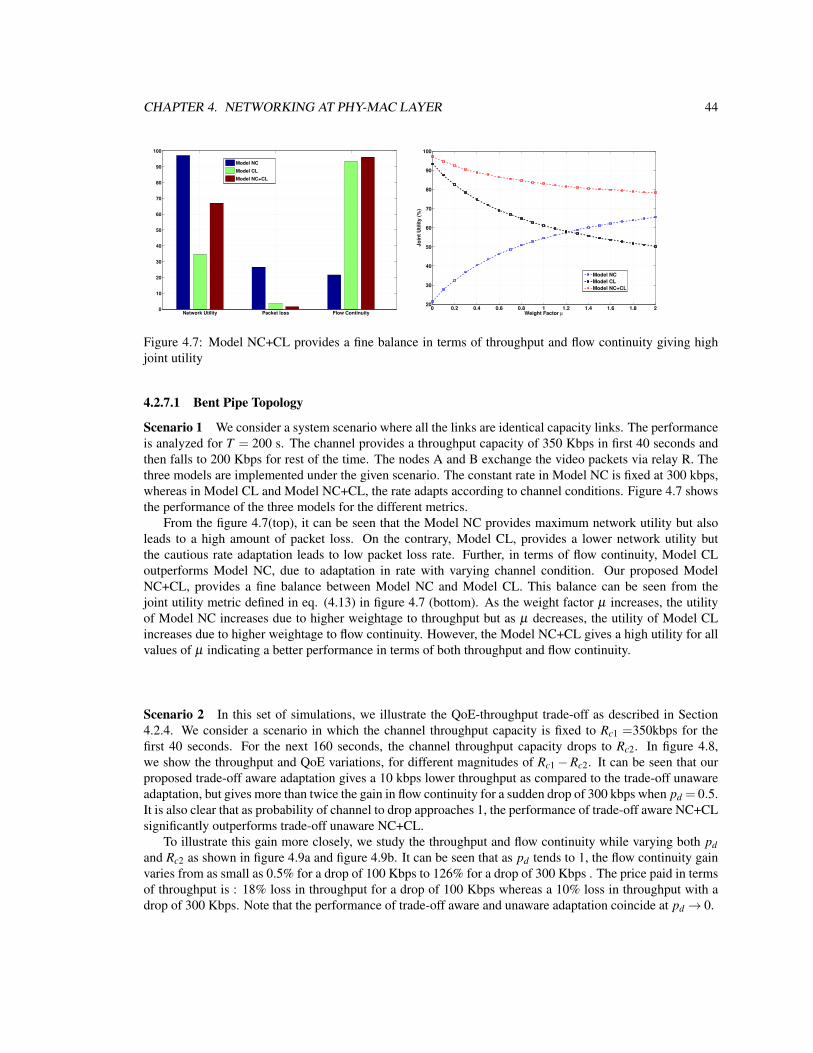
CHAPTER 4. NETWORKING AT PHY-MAC LAYER 44
Network Utility Packet loss Flow Continuity0
10
20
30
40
50
60
70
80
90
100
Model NC
Model CL
Model NC+CL
0 0.2 0.4 0.6 0.8 1 1.2 1.4 1.6 1.8 220
30
40
50
60
70
80
90
100
Weight Factor µ
Jo
int
Uti
lity
(%
)
Model NC
Model CL
Model NC+CL
Figure 4.7: Model NC+CL provides a fine balance in terms of throughput and flow continuity giving highjoint utility
4.2.7.1 Bent Pipe Topology
Scenario 1 We consider a system scenario where all the links are identical capacity links. The performanceis analyzed for T = 200 s. The channel provides a throughput capacity of 350 Kbps in first 40 seconds andthen falls to 200 Kbps for rest of the time. The nodes A and B exchange the video packets via relay R. Thethree models are implemented under the given scenario. The constant rate in Model NC is fixed at 300 kbps,whereas in Model CL and Model NC+CL, the rate adapts according to channel conditions. Figure 4.7 showsthe performance of the three models for the different metrics.
From the figure 4.7(top), it can be seen that the Model NC provides maximum network utility but alsoleads to a high amount of packet loss. On the contrary, Model CL, provides a lower network utility butthe cautious rate adaptation leads to low packet loss rate. Further, in terms of flow continuity, Model CLoutperforms Model NC, due to adaptation in rate with varying channel condition. Our proposed ModelNC+CL, provides a fine balance between Model NC and Model CL. This balance can be seen from thejoint utility metric defined in eq. (4.13) in figure 4.7 (bottom). As the weight factor µ increases, the utilityof Model NC increases due to higher weightage to throughput but as µ decreases, the utility of Model CLincreases due to higher weightage to flow continuity. However, the Model NC+CL gives a high utility for allvalues of µ indicating a better performance in terms of both throughput and flow continuity.
Scenario 2 In this set of simulations, we illustrate the QoE-throughput trade-off as described in Section4.2.4. We consider a scenario in which the channel throughput capacity is fixed to Rc1 =350kbps for thefirst 40 seconds. For the next 160 seconds, the channel throughput capacity drops to Rc2. In figure 4.8,we show the throughput and QoE variations, for different magnitudes of Rc1−Rc2. It can be seen that ourproposed trade-off aware adaptation gives a 10 kbps lower throughput as compared to the trade-off unawareadaptation, but gives more than twice the gain in flow continuity for a sudden drop of 300 kbps when pd = 0.5.It is also clear that as probability of channel to drop approaches 1, the performance of trade-off aware NC+CLsignificantly outperforms trade-off unaware NC+CL.
To illustrate this gain more closely, we study the throughput and flow continuity while varying both pdand Rc2 as shown in figure 4.9a and figure 4.9b. It can be seen that as pd tends to 1, the flow continuity gainvaries from as small as 0.5% for a drop of 100 Kbps to 126% for a drop of 300 Kbps . The price paid in termsof throughput is : 18% loss in throughput for a drop of 100 Kbps whereas a 10% loss in throughput with adrop of 300 Kbps. Note that the performance of trade-off aware and unaware adaptation coincide at pd → 0.

CHAPTER 4. NETWORKING AT PHY-MAC LAYER 45
80 100 120 140 160 180 200 220 240 260 280 30080
100
120
140
160
180
Drop in Channel Capacity (Kbps)
Thro
ughput (in K
bps)
80 100 120 140 160 180 200 220 240 260 280 3000.2
0.4
0.6
0.8
1
Drop in Channel Capacity (Kbps)
Flo
w C
ontinuity
Trade−off aware NC+CL, pd = 0.1
Trade−off aware NC+CL, pd = 0.5
Trade−off aware NC+CL, pd = 0.9
Trade−off unaware NC+CL
Figure 4.8: The higher the drop, the better QoE for trade-off aware adaptation with smaller throughputcompromise.
00.1
0.20.3
0.40.5
0.60.7
0.80.9
1
50
100
150
200
80
90
100
110
120
130
140
150
160
170
Estimated probability of channel dropChannel capacity value after drop
thro
ug
hp
ut
(Kb
ps)
90
100
110
120
130
140
150
160
Traditional QoE based Adaptation
Trade−off Aware Adaptation
(a) The smaller the drop from Rc1 = 350kbps, the better is thethroughput
00.1
0.20.3
0.40.5
0.60.7
0.80.9
1 50
100
150
200
0.4
0.5
0.6
0.7
0.8
0.9
1
dropped channel capacity value (kbps)estimated probability of channel drop
flo
w c
on
tin
uit
y
0.4
0.5
0.6
0.7
0.8
0.9
Standard QoE based Adaptation
Trade−off aware adaptation
(b) Trade-off aware adaptation gives better flow continuity
Figure 4.9: Comparison of throughput and flow continuity for varying channel capacity drops and varyingprobability of drop

CHAPTER 4. NETWORKING AT PHY-MAC LAYER 46
Network Throughput Utility Flow Continuity0
10
20
30
40
50
60
70
80
90
100
Perc
en
tag
e (
%)
NC
CL
NC+CL
NCCL with NC
NCCL with CL
(a) Destinations located such that there is no loss of over-hearing
Network Throughput Utility Flow Continuity0
10
20
30
40
50
60
70
80
90
100
Perc
en
tag
e (
%)
NC
CL
NC+CL
NCCL with NC
NCCL with CL
(b) Destination nodes located such that there is an interme-diate loss of overhearing.
Figure 4.10: Performance Comparison in terms of QoS (Network Throughput) and QoE (Flow continuity).Note that in case there is no loss in overhearing, the switching mechanisms are not utilized .
4.2.7.2 X-topology
In this section, we will present the numerical simulations to illustrate the performance of different models inX-topology.
Performance Comparison of Models On the basis of the performance metrics described in section 4.2.6,we now compare the models NC, CL and NC+CL along with the different switching in X-topology. Weconsider synthetic channel traces for a span of 1000 time slots. The channel capacity is initially 350 Kbps forfirst 250 seconds, then drops to 200 kbps for 250 seconds, again rises to 350 Kbps for next 250 seconds anddrops for 200 Kbps for last 250 seconds. The initial rate is set to 150 Kbps.
In figure4.10a, we show the network throughput utility and flow continuity performance of differentmodels in case the destination nodes are at a fixed geographical location, such that the overhearing capacityof the links RO is high and the source rate never exceeds it. It can be seen that the network utility of ModelNC exceeds that of Model CL, and flow continuity of Model CL exceeds that of Model NC. However, ModelNC+CL provides a fair trade-off between the two. Also it can be seen, that the Model NC+CL has the sameperformance with or without switching because there is no loss of overhearing and there is no switchingrequired.
In figure4.10b, we compare the performances of the models when the destination nodes are placed suchthat the overhearing capacity between the source and the destination RO , is fixed at 220 kbps. Hence,the Model NC+CL switches to Model NC or Model CL. It can be seen in figure4.10b, that NC+CL withNC-based switching, outperforms NC+CL with CL-based switching in case of network throughput utility,whereas CL-based switching in NC+CL marginally outperforms the NC-based switching in terms of flowcontinuity. However, switching between models outperform Model NC+CL without switching in all cases.
Location based variation of QoS and QoE in NC+CL Models with switching In this set of simulations,we focus upon the performance of NC+CL model and illustrate the variation in performance for differentlocations of the destination nodes. As we consider symmetric model, we plot the geographical distribution ofone pair (S1-D2 or S2-D1). We place the source node at the origin and place the unintended destination nodeat different integral coordinates on a space where both x-coordinate and y-coordinate vary from -500 km to500 km.

CHAPTER 4. NETWORKING AT PHY-MAC LAYER 47
−5
0
5
x 105
−5
0
5
x 105
38
40
42
44
46
48
X−coordinate (in metres)Y−coordinate (in metres)
Qo
S (
in %
)
39
40
41
42
43
44
45
46
47
(a) QoS Performance of NC+CL with NC-based switch-ing
−5
0
5
x 105
−5
0
5
x 105
99
99.2
99.4
99.6
99.8
100
X−coordinate (in meters)Y−coordinate (in meters)
Qo
E (
in %
)
99
99.1
99.2
99.3
99.4
99.5
99.6
99.7
99.8
99.9
100
(b) QoE performance of NC+CL with NC based switch-ing
Figure 4.11: QoS and QoE variation in Model NC+CL with NC-based switching for different geographicalplacements of destination nodes
−5
0
5
x 105
−5
0
5
x 105
36
38
40
42
44
46
48
X−coordinate (in meters)Y−coordinate (in meters)
Qo
S (
in %
)
38
39
40
41
42
43
44
45
46
47
(a) QoS performance variation
−5
0
5
x 105
−5
0
5
x 105
99.26
99.27
99.28
99.29
99.3
99.31
99.32
99.33
X−coordinate (in meters)Y−coordinate (in Meters)
Qo
E (
in %
)
99.27
99.275
99.28
99.285
99.29
99.295
99.3
99.305
99.31
99.315
99.32
(b) QoE performance variation.
Figure 4.12: QoS and QoE variation in NC+CL with CL-based switching for different geographical place-ment of destination nodes
In figure4.11, we show the variation of QoS and QoE at different geographical locations with NC-basedswitching with NC+CL model. It can be seen that the QoE decreases towards the origin where the overhearingcapacity is higher (close to the source). This is due to the fact that with higher overhearing, there are morechances of network coding, which optimizes QoS. As expected, the QoS close to the origin is highest and itreduces as the node moves away from the source.
In figure4.12, we show the variation of QoS and QoE at different geographical locations with CL-basedswitching in NC+CL Model. As opposed to NC-based switching, the overall QoE is higher in this case,although the gradient decreases away from center. This is because, whenever overhearing is lost, CL opti-mization ensures a high QoE. The QoS profile remains the same, with a lower magnitude due to no use ofNC after loss of overhearing.
In order to compare the performance of the two switching mechanisms in NC+CL model, we plot theoptimal switching with NC+CL model in terms of QoS and QoE, for different locations of the node. As shownin figure4.13, the dominant switching in most locations for optimal QoS is NC-based switching, whereas thedominant switching mechanism for optimal QoE is CL-based switching.

CHAPTER 4. NETWORKING AT PHY-MAC LAYER 48
−5 −4 −3 −2 −1 0 1 2 3 4 5
x 105
−5
−4
−3
−2
−1
0
1
2
3
4
5x 10
5
X coordinate
Y c
oo
rdin
ate
NC+CL with CL
NC+CL with NC
(a) QoS optimal model for different regions
−5 −4 −3 −2 −1 0 1 2 3 4 5
x 105
−5
−4
−3
−2
−1
0
1
2
3
4
5x 10
5
X coordinate
Y c
oo
rdin
ate
NC+CL with NC
NC+CL with CL
(b) QoE-optimal model for different regions
Figure 4.13: Location-optimal Model Map: the optimal switching to be applied at different geographicalplacement of destination node.
However, there are some exceptional places towards the boundary of the space, where NC-based switch-ing is dominant strategy for both high QoE and QoS. This is due to the following reason: as the distanceof the destination node from the origin increases, the overhearing capacity decreases. Towards the boundaryof space, the overhearing capacity reduces to be less than the channel capacity after the drop has occurred.Therefore, in case the source rate reaches the overhearing capacity (which is very low), in NC-based switch-ing, the transmission occurs at low rate. However, no delay is seen by the receiver. In case of Model CL,the rate is adapted gradually, which results in delay and packet losses when the source rate exceeds the net-work capacity. Therefore, in such geographical regions, with low overhearing capacity, NC-based switchingoutperforms CL-based switching in terms of QoE. Another exception is, for a circular ring of width 100 km,there is a region where CL based switching is optimal for both QoS and QoE. The reason is as follows: theaverage QoS is directly proportional to the number of packets obtained at the receiver and inversely propor-tional to the time taken to deliver those packets. With NC model, a reduced number of time slots is requiredfor transmission, which leads to gain in QoS as opposed to CL model at comparable rates. However, whenthe rates in model CL are much higher as compared to model NC, the gain in QoS due to reduced numberof time-slots does not outperform the gain in CL due to higher rate. In this region, the source rate exceedsthe overhearing capacity at a value such that the amount of gain using CL is more than the reduced time slotutilized using NC.
Hence, this demonstrates that in order to supply an optimal QoS and/or QoE to the user, the serviceprovider should consider the location of the users, and choose the optimal model for the same.
4.3 Maximizing throughput using cognitionWe will now present another contribution towards the networking techniques for satellite networks with theaim of maximization of throughput. The aim of this study is to analyze the networking techniques using theconcept of cognitive radio in satellite scenarios. The use of cognition is well-known to optimize resourceutilization and enhance the performance and it is a promising technique for future wireless networking.

CHAPTER 4. NETWORKING AT PHY-MAC LAYER 49
(a) Monobeam and Multibeam Coexisting DSS (b) NGEO and GEO coexisting DSS (c) Overlapping coverage DSS
Figure 4.14: Some typical DSS scenarios
4.3.1 Concept of CognitionThe concept of cognition was proposed in the seminal paper of Mitola in 1999 [74]. It was further applied towireless communications by Haykin in 2005 in [75] where he applied cognition to radio spectrum utilizationand coined the term cognitive radio. Haykin defines cognitive radio as follows [75]:
Cognitive radio is an intelligent wireless communication system that is aware of its surrounding en-vironment (i.e., outside world), and uses the methodology of understanding-by-building to learn from theenvironment and adapt its internal states to statistical variations in the incoming RF stimuli by making corre-sponding changes in certain operating parameters (e.g., transmit-power, carrier-frequency, and modulationstrategy) in real-time, with two primary objectives in mind:
• highly reliable communications whenever and wherever needed,
• efficient utilization of the radio spectrum.
Cognitive radio (CR) therefore provides intelligent transmission protocols in which the communication isassociated with observation of the available resources dynamically and efficiently, processing the observationand acting based on this processing in order to provide seamless services with limited resources. Cognitioncan therefore be naturally applied in satellite networks to adapt to changing conditions and demands.
4.3.2 Dual Satellite Systems4.3.2.1 Scenarios
Dual Satellite System (DSS) is the satellite network which has two satellites operating simultaneously over acoverage area in a same spectrum band. In such systems, the two satellites share spatial and spectral degreesof freedom. The DSS models a number of satellite scenarios as follows:
• Mono-beam and Multi-beam co-existent DSS - The traditional monobeam satellites can coexist withthe multibeam satellites thereby forming a DSS. An example of such systems has been shown in figure4.14a. The users in coverage area of these two satellites may or may not be served by both the satellites.
• NGEO and GEO co-existent DSS - The GEO satellites can coexist with LEO/MEO satellites (alsocalled the Non-GEO Satellites (NGEO)) forming a DSS. An example of such systems has been shownin figure 4.14b. Since GEO satellites cover a fixed geographical area all the time, whereas NGEOsatellites may cover the same area over some period of time, the two satellites are required to coexist.Such coexisting systems need to combat not only the interference due to the signals from co-locatedsatellites, but also the inline interference due to loss of line of sight of GEO owing to NGEO.

CHAPTER 4. NETWORKING AT PHY-MAC LAYER 50
• Overlapping coverage DSS - Two similar satellites having overlapping coverage areas form a DSS.Due to increasing space traffic and high demands, a number of satellites are being deployed for differ-ent specific purposes and/or are deployed in close proximities. This leads to the overlapping area ofcoverage. An example of such scenarios has been shown in figure 4.14c.
• Replacement phase DSS - During the replacement phase of an old satellite with a new satellite, thereare long phases of coexistence before the old satellite is completely eliminated from the orbit. Suchreplacement phases form a system when the two satellites coexist thereby forming a DSS.
It is clear that the DSS can model a number of satellite scenarios and therefore, the utility of study of theDSS is imperative. There are a number of existing satellite systems which can be analyzed as DSS. Forexample, the Other Three Billion network proposed O3b satellites in the MEO due to the advantages of MEOsatellites like reduced free space attenuation, small propagation delay and reduced in-orbit injection cost [76].However, these satellites use parts of Ka band which is also being used by GEO satellites thereby forminga DSS as studied in [77]. Similar example of LEO and GEO coexistent network is IRIDIUM constellationwhich consists of a network of 66 LEO satellites coexisting with GEO satellites in different coverage areas[78]. An example of replacement phase DSS is the replacement of existent Iridium network with the IridiumNEXT constellation (to be launched in 2015) which aims to replace the older network completely by 2020[79]. Therefore, both Iridium and Iridium Next with form a DSS for approximately 5 years. Other examplesof such DSS are NGEO satellite networks like Orbcomm and Globestar coexisting with the GEO satellites.
4.3.2.2 Challenges
The DSS described above possess some inherent challenges/limitations which are required to be addressedfor an optimal utilization.
1. Limited Spectrum: The DSS consists of two satellites sharing the spectral degree of freedom. With thehigh amount of space traffic, the problem of spectrum scarcity is well known [65]. Therefore, the DSSneeds an efficient and optimal technique for utilizing the available spectrum. For example, by ITU RRNo. 5.523A, certain parts of Ka band have been assigned to GEO satellites. However, some of theupcoming satellite networks of NGEO satellites utilize those parts of spectrum for their transmission.This leads to spectrum sharing which is an important challenge which is needed to be addressed inDSS.
2. High interference: In the coexistence of two satellite networks sharing both spatial and spectral domain,there is an important problem of interference between two networks which is required to be addressed.The interference in DSS can be classified in two categories. Firstly, the interference arising fromthe wireless signals of the two coexisting networks. This interference is constantly present and isrequired to be tackled by interference mitigation techniques like interference alignment, beamforming,precoding etc. Secondly, the interference which arises in DSS due to the orbital position of the satellitesleading to inline-interference. This type of interference is observed in DSS formed by GEO and NGEOsatellites when NGEO satellite falls in line of sight of the GEO satellite and its ground terminal.
3. Low Channel Availability: The DSS faces an important challenge of the availability of wireless chan-nels because two systems sharing a limited spectrum coexist. This problem is specifically importantin Land mobile satellite (LMS) scenarios, although it also exists in Fixed Satellite Scenarios (FSS).In LMS scenarios, the channel conditions between the satellites and the ground terminal varies con-tinuously, hence the joint effects of shadowing of channel and uncoordinated sharing of the availablechannel with the other satellite network leads to low channel availability. The low channel availabilityin such scenarios has been well studied in [80, 81].

CHAPTER 4. NETWORKING AT PHY-MAC LAYER 51
Figure 4.15: Proposed Block Diagram for Cognitive Cycle
4.3.3 Cognition in DSS4.3.3.1 Proposed Cognitive Cycle
The concept of cognition is applied to the communication systems using a precise cognitive cycle [82]. Thecognitive cycle proposed here is shown in figure 4.15. The cognitive radio node in the network observes orsenses the external environment stimulus. The sensed data is processed and based on the processed data, themost efficient action is taken in order to achieve the aim. This process leads to enhancement of performancein order to achieve the predefined aim. This cognitive cycle shows the basic steps of cognitive radio, namely,observe-process-act.
Furthermore, in cognitive scenario, users are classified as primary users (PU) and secondary users (SU).The PU are the incumbent users which are given a priority in the cognitive transmission and it is ensured thattheir services are not disrupted due to the presence of other systems. The SU are the users which use thecognitive techniques and adapt themselves to coexist with PU without lowering the quality of services of PU.For example, in hybrid satellite terrestrial networks, the terrestrial network is (typically) considered as PUand the satellite network utilizes the resources to provide the services to its users without compromising theservices of terrestrial networks.
In the seminal paper of [74] on cognitive radio based communications, Mitola describes the implementa-tion of communication based on cognition to be driven by the repeated stimulus from external environment.Such stimuli leads to series of ’intelligent’ techniques employed for efficient and adaptive communications.The continuous stimuli observation and cognitive actions lead to a cognitive cycle. Inspired by Mitola’s Cog-nitive cycle based communications, we propose a cognitive cycle to assess the concept of communicationapplied to the DSS. The cognitive cycle has been shown in figure 4.15.
The CR in satellite communication systems could be employed at either ground terminal or the satelliteterminal depending on both, the requirements and the feasibility [83]. The cognitive radio (CR) is comprisedof the basic cycle of observe-process-act. Each of the steps of the figure 4.15 are explained below.
• Independent of the terminal used for cognition, the cognition is employed with a predeterminedaim/target, just as any intelligent or brain-empowered action is performed with an aim or a set mo-tive. The aim for cognition further drives the CR.
• The primary requirement of cognition is the observation of external stimuli. The external stimuliobservation implies monitoring the available information of the radio environment.

CHAPTER 4. NETWORKING AT PHY-MAC LAYER 52
Figure 4.16: Translation of different steps of Cognitive Cycle into Engineering Design Steps
• Using the stimulus (raw data) which is sensed from the environment, the CR stores the sensed data indatabases. Such data is processed and quantified using appropriate metrics. Such information is againstored in the database, analyzed and classified into different categories.
• Based on this classification, it is determined what cognitive action should be taken in order to realizethe initial aim of the cognition and when such an action should be taken. Cognition also implies thatthe processed information is constantly monitored to determine the expected trend of the stimulus andimplement the suitable action.
• Furthermore, this cognitive cycle of observe-process-act is performed repeatedly during the transmis-sion to realize the aim of cognition. The overall improvement from this cognitive cycle results is mea-sured on the basis of different performance metrics like spectral efficiency, power efficiency, diversityetc.
4.3.3.2 Cognitive Cycle from Engineering Design Perspective
The challenges in DSS are required to be addressed in order to tap the potential of DSS in increasing boththe quality of service and efficiency of resource utilization. Cognitive radio promises to be an efficientsolution. This is because precisely each step of the cognitive cycle can be mapped into an engineering designrequirement and can be tackled using accurate methods. The different phases of cognitive cycle proposedin figure 4.15 can be mapped to different phases of engineering design problem as shown in figure 4.16.The basic aim of cognition can be translated as the system design objective from perspective of engineeringdesign. Furthermore, the radio-electric sensor outputs serve as cognitive stimulus which can be sensed andprocessed using signal processing and optimization techniques. The cognition-driven action can be furtherseen as the engineering/transmission techniques used for the communication leading to fulfillment of designobjective. Such a precise mapping indicates that the realization of the abstract principles of cognitive cycleinto practical implementation can be translated with concrete and well defined steps. It also reaffirms theapplicability of cognition in satellite networks like DSS because in such systems, precise and robust protocolsare required due to cost benefits and complexity involved.
There are a number of cognitive DSS studied in literature. Based on the proposed cognitive cycle, eachof the these cognitive DSS can be categorized to be associated with different aim of cognition. The differentsteps followed to achieve this aim can be associated with different phases of the proposed cognitive cycle(Table 4.1). We now develop a taxonomy of the different existing cognitive DSS and identify the phases ofcognitive cycle proposed with different steps taken in each of these cognitive DSS categories.
The existent cognitive DSS can be divided into three categories:
1. Spectrum Management based Cognitive DSS
2. Interference Management based cognitive DSS

CHAPTER 4. NETWORKING AT PHY-MAC LAYER 53
!"#$%&$'%()"*%)$
'%()"*+,$$-*#./.-$
0,)-,$12324$-3%52(,$2)1$65%7,--")($
'%()"*+,815"+,)$27*%)$
9,5&%5#2)7,$#,35"7$3%$:,$"#65%+,1$
!"#$%&'%(')%#*$+,(-%+'%(
./(0)%#*$+,(+1234&15"(6/(752&$34&15"(+1234&15"(
./ 08'*%,9:;&""%2(<5=%23">((
6/ :5,)+*%(75?%$(0)%#*$&2(@%"'3*8((
A/ !,)2%,%"*(&2>5$3*;,'(5B(&"&28'3'(
./ <+21)2%C3">(6/ 0#;%=+23">(A/(D$&"',3''35"(3"(0)%#*$+,(;52%'(
./ 0)%#*$&2(%E#3%"#8(
6/ 75?%$(%E#3%"#8(
F)1,34%(3"*%$B%$%"#%(,&"&>%,%"*(
!"*%$B%$%"#%(( ./ 08'*%,9:;&""%2(<5=%23">(
6/ :5,)+*%(!"*%$B%$%"#%(D%,)%$&*+$%(
A/ :2&''3B8(3"*%$B%$%"#%(2%G%2'(
./ !"*%$B%$%"#%(&23>",%"*(
6/ 7$%#5=3">(A/ H%&,B5$,3">(I/ -&*%(')23J">(
./ 0)%#*$&2(%E#3%"#8(
6/ 75?%$(%E#3%"#8(
!"#$%&'%('8'*%,(&G&32&K323*8(
:;&""%2(LG&32&K323*8(
./ 08'*%,9:;&""%2(<5=%23">(
6/ :5,)+*%(0;&=5?3">(*;$%';52=(
A/ !,)2%,%"*(&2>5$3*;,'(*5(#2&''3B8(';&=5?3">(
./ <!<F(D%#;"3M+%'(
6/ N%*?5$O(:5=3">(
@3G%$'3*8(P0)&1&2Q(D%,)5$&2Q(L">+2&$R(
0;-3,#$<,-"()$%:=,7*+,$
>21"%8,/,735"7$-,)-%5$%.36.3$
0"()2/$65%7,--")($2)1$%6*#"?2*%)$
@)("),,5")(A352)-#"--"%)$3,7B)"C.,$
D./E//#,)3$%&$1,-"()$%:=,7*+,$
Table 4.1: Taxonomy of Different cognitive techniques based on the aim of cognition. The columns withineach row indicate the phases of cognitive cycle related to each aim of cognition. The top row shows the stepsof cognitive cycle and the bottom row indicates the engineering design equivalent of each step.
3. System Availability based cognitive DSS
In the next subsections, we explain each of these categories in detail.
4.3.4 Taxonomic Analysis of Cognitive DSSWe have seen that there are a number of scenarios where DSS arise and they can be modeled in differentways. In addition, in order to ensure an efficient coexistence of two satellite systems in a DSS, cognitivetechniques have been shown to be very useful as described in section 4.3.3. In this section, we explore ataxonomy of the cognitive techniques applied to DSS.
4.3.4.1 Spectrum Management based Cognitive DSS
The cognitive DSS which employ cognitive techniques to deal with the problem of scarce spectrum fall in thiscategory. The under utilization of spectrum in satellite systems has been well pointed out in [63]. The twosatellite systems in DSS share a spectrum which leads to necessity of intelligent techniques to manage thelimited available spectrum. The use of such cognitive techniques [83] entails all the steps of cognitive cycleand the engineering design equivalent as explained further. All the DSS models explained in section 4.3.2.1and section ?? can be used to implement these techniques. In general, the multibeam/monobeam coexistenceDSS considers monobeam satellite as PU. In NGEO/GEO coexistence DSS, GEO satellite is considered asPU.
Cognitive Stimulus In order to implement the cognitive techniques with an aim of spectrum management,the external stimulus sensed by the satellite system is the availability of free spectrum. This is the primary stepof sensing the spectrum using an appropriate spectrum sensing technique. There are a number of spectrum

CHAPTER 4. NETWORKING AT PHY-MAC LAYER 54
sensing techniques which are provided in the literature, not specific to DSS, but are applicable in all multi-satellite scenarios [64, 65, 66]. The three mainly used signal processing techniques for sensing are MatchedFilter Detection, Energy Detection and Cyclostationary feature detection [84]. However, these techniquesare limited by received signal strength which cannot be guaranteed in variable environment. In such cases,cooperative sensing is more efficient.
Storage and Processing After sensing the spectrum utilization (both spatially and temporally), the sensedspectrum is quantized using the metrics like power spectral density (PSD). Based on the PSD, differentalgorithms are applied to identify if the PSD observed indicates presence of PU with certain probability ofdetection. In addition, the spectral usage in space-time-frequency domain identified via the spectrum sensingtechniques can be classified into three different categories [83]: (a) Black Space - spectral portion occupied byhigh power satellites or local interferes some of the time, (b) Grey Space - spectral portion which are partiallyoccupied by low power interferers and (c) White Space - spectral portion free of RF interferers except forambient noise consisting of natural and artificial forms of noise. In the different DSS scenarios, the SUtransmits in preferably white space using the opportunistic transmission. To transmit in grey or black spaces,an appropriate interference management technique is required, which will be discussed in next subsection.It should be noted that the opportunistic transmission in spectral holes also includes the transmission in 3Dspace spectral holes. This implies that the spectral holes can be identified depending on transmission angleand polarization, and such parts of spectrum can also be opportunistically utilized for cognitive transmission.
Cognitive technique The cognitive-driven action or the transmission techniques for spectrum managementcan be studied under two categories:
1. Opportunistic Transmission: A very basic and very effective cognitive technique applied to DSS isthe opportunistic transmission by secondary user in the spectrum holes of the primary user. Morespecifically, the CR terminal at the SU utilizes the radio spectrum on a non-interfering basis in a spatio-temporal manner by giving a higher priority to incumbent spectral users.
An implementation of opportunistic transmission technique has been studied in [85] using the con-cept of cognitive beamhopping in overlapping coverage coexistent DSS. The primary satellite networkis allowed to transmit at a predetermined spectrum bandwidth. However, there is dynamic spectrumsensing applied at the SU and the idle bands are assigned to the SU. In a traditional beamhopping sys-tem, each active beam uses full frequency instead of fractional frequency reuse as in the conventionalmultibeam systems. This property is exploited in the cognitive beamhopping DSS. Since only a certainfraction of total available beams are active in a particular time slot, the unused frequencies can be usedby secondary satellite network of DSS. Basically, the primary satellite system is a beamhopping systemwith larger beams. The secondary satellite system can also be considered to be a beamhopping systemwith smaller beams and lower peak power.
2. Cooperative Transmission: Conventional techniques of spectrum management are cognitive in nature,namely multiplexing and scheduling. In case of cognitive DSS (e.g.. in case of NGEO/GEO coexis-tence), the spectrum can be shared between PU and SU to an extent that is within tolerable limits of PU.The resources can be shared in frequency (Frequency Division Multiplexing) or time (Time DivisionMultiplexing). Furthermore, in case of monobeam/multibeam coexistence DSS, in the uplink, spec-trum assignment based on the demands of the users which adds another level of cognitivity to spectrummanagement. Such a case has been very well presented in [86] and can be applied straight-forward tothe DSS.
The output of these spectrum management cognitive techniques is a reduction in spectrum scarcity which canbe measured using the metrics such as spectral efficiency or power efficiency.

CHAPTER 4. NETWORKING AT PHY-MAC LAYER 55
4.3.4.2 Interference Management based Cognitive DSS
The cognitive DSS which employs the cognitive techniques with the aim of interference management arecategorized under this subsection. The spectral coexistence of two satellite systems in DSS can be modeledas Cognitive Radio (CR) network with interference channels between primary and secondary systems. Anumber of interference management techniques are employed in cognitive DSS in order to reduce/eliminatethe interference of SU towards the PU while maintaining the QoS of the SU. It should be pointed out here thata cognitive system should be also able to embrace interference. Such techniques can be also studied in-linewith our proposed cognitive cycle as follows:
Cognitive Stimulus The external stimulus used to assess the implementation of cognitive techniques tocombat interference is the radio-electric sensing of interference at the primary user node. This is preciselydone by assessing the radio-electric signals obtained at the PU. These signals are observed over stipulateddomains of time/space/frequency before proceeding to the next step.
Storage and Processing data The observed signals are further stored and processed to assess the amountof interference in at the PU. This processing involves quantization of observed signals to identify interference.The FCC task force report [63] defines the metric of interference temperature to model the interference facedby the PU from the SU. Hence in cognitive DSS, the interference management techniques aim to ensure thatthe interference temperature at the PU does not exceed a predetermined threshold.
Cognitive technique The interference management techniques considered in cognitive DSS can be stud-ied under two sub-categories: Interference management via flexible/beamforming system: The interferencemanagement depending on the domain used has been extensively explored in [87] using beamforming tech-niques. These techniques are valid for all the scenarios discussed above in downlink transmission. In [88]and [77], these techniques are studied for DSS. Note that in these techniques, we assume that the interferencemanagement is used at both primary SAT1 and Secondary SAT2.
1. Interference Alignment: The basic principle of IA is based on aligning the interference on a signalsubspace with respect to the non-intended receiver, so that it can be easily filtered out by sacrificingsome signal dimensions. The fundamental assumptions which render IA feasible are that there aremultiple available domains (space, frequency,time or code) and that the transmitter is aware of the CSItowards the non-intended receiver. Interference Alignment (IA) in satellite system was initially studiedin [89] for downlink scenarios. It was also proved in this work that subspace interference alignmentis feasible in downlink satellite scenarios using only certain geometrical arrangement constraints. IAwas later studied in uplink transmission because in downlink, in general, the coverage of the satellitesis geographically large and it is complex to align the signal from satellite in certain dimensions forthe terrestrial receivers. DSS had later been discussed in [88] for uplink transmission in which IA isapplied to multibeam satellite terminals to mitigate interference towards monobeam satellite. Further,depending on the degree of cognition, different IA techniques are possible:
(a) Static IA: The simplest case of IA employed at the ST2’s is based on the initial concept of IAintroduced in [90] according to which a non-zero reference vector v is chosen along which theinterference should be aligned. The selection of alignment direction can be predetermined withsignaling from intended gateway. The interference aligned across v can be removed using zero-forcing filter. This basic IA approach leads to a unit multiplexing gain and is not optimal.
(b) Coordinated IA: Adding more amount of cognition to IA leads to coordinated IA, where theprimary and secondary systems coordinate to exchange CSI information and the alignment vectordynamically depending on best conditions.

CHAPTER 4. NETWORKING AT PHY-MAC LAYER 56
(c) Uncoordinated IA: In this approach cognition is on side of PU and the primary and secondarysystems do not coordinate. The ST2s choose the v to maximize their throughput and subsequently,SAT1 senses the v and applies the appropriate filter.
Further, in [91] IA techniques with frequency packing have been suggested which involves reducingspacing between adjacent signals in the frequency domain, while employing advanced techniques forsuppressing or exploiting the additionally reduced interference.
2. Interference mitigation by power control: The DSS also faces another type of interference namelyinline interference, which is particularly significant in NGEO-GEO coexistence scenarios. CognitiveDSS employ inline interference mitigation by power control techniques. The GEO satellite systemis considered the primary system and the NGEO satellite system is considered as the secondary user.Such scenarios have been shown in figure 4.14b. The interference mitigation is tackled by formulatingoptimization problems for uplink and downlink separately [77]. In uplink transmission, the optimiza-tion problem for power allocation requires the NGEO earth station (ST2) to control its transmit powersuch that the interference at the GEO satellite terminal (I/N)sat1 is below the threshold level whilesimultaneously ensuring its own QoS. In downlink transmission, the optimization problem for powerallocation requires the NGEO satellite (SAT2) to transmit at power levels such that the NGEO termi-nals (ST2) on ground obtain the desired (C/N)st2 ratio whereas the GEO terminals on the ground (ST1)have the (I/N)st1 below the threshold level. Furthermore, the on-board power constraint of the NGEOsatellite should be satisfied.
4.3.4.3 System Availability based Cognitive DSS
Assessing how to improve the availability is a problem that has to be often tackled whenever two systemssharing a limited spectrum coexist, as is the DSS case. Developing efficient techniques becomes even ofmore importance when the scenario is mobile, i.e. LMS-DSS, which means that besides of sharing thespectrum users have limited and time varying visibility of the satellites, i.e. limited and varying spectrumholes from which to send or gather the data. Although there exist no specific works assessing the LMS-DSS scenario, it is well known that Network Coding (NC) and Multiple Input Multiple Output (MIMO)techniques can help to improve the availability in mobile scenarios. These techniques are based on the ideaof embracing interference rather than mitigating it as pointed out in section 4.3.4.2. We have explored indetail the implication of LMS-DSS with these techniques in [73] which interested readers may refer to.
4.4 Concluding remarks
4.4.1 Contributions over state-of-the-artIn this chapter, we have taken a very elaborate view of the different networking techniques applied beyondpurely physical layer at the PHY/MAC layer. At this layer, we considered the target wireless scenarios to beeither general relay scenario or satellite scenarios to focus on accurate wireless model for our study. Thesenetworking techniques have been studied to be applied in coherence with two aspects of communications.
• The first part of our studies has shown application of network coding at link layer along with QoE-driven cross application/transport layer optimization. This work develops a novel scheme to implementQoE-driven cross-transport/application layer optimization using network coding at the network layerfor video transmission in a wireless relay network. This work also presents novel trade-offs whichare a crucial consideration for design of such schemes. Another important contribution of this workis the use of novel geographical distribution based tools to optimize the joint implementation of suchschemes whose potential has not been exploited in literature so far.

CHAPTER 4. NETWORKING AT PHY-MAC LAYER 57
There are research work aiming at joint implementation of different types of cross layer optimizationschemes with network coding [55, 54]. Our work departs from the state-of-the-art due to the use of thecross transport/Application layer optimization which is transparent to the network coding at lower lay-ers. Furthermore, we have shown the implication of the use of QoE-driven cross-layer adaptation andthe effective end-user perception with network coding, which is a novel contribution. We illustrate thatthe joint implementation of CL and NC in X-topology and in bent-pipe topology, using Model NC+CLleads to the existence of a QoE-throughput trade-off. This trade-off is crucial for choosing the optimalparameters to achieve desired performance. Furthermore, we also used the location of the terrestrialusers to optimize the throughput by adapting the transmission rate to the user-location constraint. Theextra information conveyed due to user location further consolidates the overall performance in termsof QoE and throughput. Via numerical simulations, we illustrate that for each location of the user, anoptimal switching with NC+CL model for QoS or QoE can be identified, which should be adopted bythe service provider for maximizing its user benefits. This work provides a primary insight into thejoint practical implementation of QoE driven CL and NC and demonstrates that the interplay betweenlocation based information and the novel concepts of NC+CL should be exploited to maximize thetransmission quality in future scenarios.
• The second part of our studies entails a very extensive and critical review of the various cognitive tech-niques involved in satellite channels primarily over mac/physical layer. We focus on particular satellitenetworks in this case, namely dual satellite systems, which allows for a large arena to apply cognitionin the system. This part of the chapter has provided an introductory overview of dual satellite systems,their modeling and justified the relevance to apply cognitive communication techniques to such sys-tems. In particular, the existing trends of the research in this area have been critically reviewed andclassified based on different system design objectives. To the best of our knowledge, this is amongthe first surveys on the topic of Dual Satellite systems. An important contribution of this chapter is toprovide a concrete mapping between the phases of cognitive communication cycle and the correspond-ing phases of engineering design applied in dual satellite system thereby bridging the gap between theabstract and the practical design of cognitive techniques.
4.4.2 PublicationsThe contributions presented in this chapter have resulted in following three publications:
Book Chapter
• S. Gupta, M. A. Vázquez-Castro, R. Alegre-Godoy, “Dual Satellite Systems”, Chapter in the bookCooperative and Cognitive Satellite Systems, Elseviar 2014.
Conference Proceedings
• S. Gupta, M. A Pimentel-Niño, M. A. Vázquez-Castro, "Joint network coded-cross layer opti-mized video streaming over relay satellite channel", In 3rd International Conference on WirelessCommunications and Mobile Computing (MIC-WCMC), Valencia, June 2013.• S. Gupta, M. A. Vázquez-Castro, "Location-adaptive network-coded video transmission for im-
proved Quality-of-Experience" In 31st AIAA International Communications Satellite SystemsConference (ICSSC), Florence, (2013).
4.4.3 Future lines of workThis chapter provides a comprehensive insight into the two aspects focussed upon. A number of open chal-lenges still remain to be solved which form the possible lines of future research.

CHAPTER 4. NETWORKING AT PHY-MAC LAYER 58
• The trade-off study emerging from the joint implementation of NC and QoE driven cross transport andapplication layer rate adaptation, can be further generalized for various topologies thereby building aconcrete structure to characterize such system performances.
• The location-aware transmission in the joint implementation is a theoretical study however, a numberof practical aspects of the same remain to be seen like antenna structures for overhearing, realisticoverhearing conditions, etc.. Such a study coupled with the model presented forms an interestingfuture line of research.
• The cognitive DSS techniques have a number of technological aspects of actual implementation whichhave not yet been dealt with in the literature. These aspects will ultimately provide actual gains ofcognition based designs and hence after this conceptual/academic research in cognitive DSS, it is timefor looking into technological/implementation issues.
• In addition, using the technological assessment of cognition based design implementation, a futuredirection of work is the optimal combination of the three aims of cognition presented in this chapter.
• Another important open direction to be explored is the security issues involved in inter-system trans-mission and selection of a cognitive strategy which satisfies the security demands.
Overall this chapter is a comprehensive study of the future generation wireless networks, like satellite net-works, imbibing the aspects from different independent techniques to function in coherence and provideeffective performance improvements over state-of-the-art.

Chapter 5
Networking at Transport -Applicationlayer
5.1 IntroductionHaving explored the networking techniques at the lower layers, we now focus on the transport and applicationlayer. These layers are the ones which are perceived by the end-user more closely and it is important tomaximize the effective service provided by these layers to the users while ensuring an optimal resourceutilization as well. Therefore, in this chapter we study a particular application, aim to maximize not only thethroughput but also the end-user experience in using this application.
5.1.1 Objective and technique in overall frameworkObjective: “Maximizing the joint utility using game theoretical tools”
Recently there has been a remarkable development in video transmission over hypertext transfer protocol(HTTP) [92] which uses transport control protocol (TCP) and its variants [93]. However, video transmis-sion over TCP is the best-effort transmission which does not account for specific characteristic requirementsof multimedia applications, particularly video applications, like disruptions in user-perceived video quality,overall user satisfaction etc. In order to address different specific characteristics, several cross-layer opti-mization techniques have been proposed to optimize video transmission over wireless media [22]. Thesetechniques are based on the optimization of different aspects of the video transmission like optimization ofthe Quality of Service (QoS) [94], optimization of Quality of Experience (QoE) [95, 96, 59], optimization ofa general application oriented user satisfaction [97] etc.
An important demand of the users of the video applications is to be provided a desired quality of ex-perience of the perceived video. The QoE-driven cross-layer optimization accounts for video transmissionsuch that the perceived video quality at the end-user is optimized in terms of minimizing both distortions invideo quality and disruptions in video playback. This is because the QoE at the end user is composed oftemporal structure and spatial structure of the video. The temporal structure involves the continuity in thevideo observed at the end-user without freezing or disruptions, implying timely playback of the video. Thespatial structure involves the avoidance of formation of artifacts due to packet losses at the end user [98].An inherent benefit of focussing on QoE-driven cross layer adaptation is that it generalizes the TCP basedtransmission and hence can be adopted by the existing systems. However, the wireless nodes involved in thevideo transmission are largely distributed and are autonomous devices. Therefore, the practical dynamics of
59

CHAPTER 5. NETWORKING AT TRANSPORT -APPLICATION LAYER 60
the interaction between them is governed by their independent behaviors which maximize their individualvideo quality. This independent behavior in the interactions affects the quality of the video observed at theend user.
Our objective is to assess the affect of such interactions. In particular, in a video exchange scenariobetween two selfish autonomous users, the ability of a user to obtain a desired quality video depends on theoptimization performed by the other user. However, in order to perform such an optimization, the other userincurs some cost. This leads to a natural competition between the users which optimize the quality of videothey transmit selfishly such that they incur minimum cost but are still able to obtain a desired quality videofrom other user. This chapter addresses such competitive video exchange between two users.
Technique: Game Theory
A relevant framework to model this type of interactions is provided by game theory. A game theoreticalframework also helps to analyze the prospective benefits of possible cooperation among the nodes. The basicsof game theory have been explained in Chapter 2. We will develop an extension of the basic framework todevelop the game theoretical tool in this chapter.
Contributions
The main contributions of this work can be stated as follows[99, 100]:
• We propose a novel video exchange game between two nodes where each node seeks to optimize aQoE-dependent metric to adapt the video transmission rate to varying channel conditions while mini-mizing the cost. Particularly, we identify a natural game in which the players use the QoE-driven rateadaptation algorithm as their strategy. There is no external/artificial price mechanism used to controlthe outcome of the game.
• We analyze the possible outcomes of the game when it is played once and when it is played repeatedlyand thereby establish the clear conditions required for cooperation to be sustained for long durationusing the tools in [101]. It is shown that when the game is played once or a finite number of times, theplayers have no incentive to cooperate and rate adaptive video transmission is not sustained. However,a non-trivial solution is obtained only when the game is played repeatedly and the players are unsureof the final stage of the game. We illustrate that in such an interaction, a heterogeneous quality videoexchange between two users can be sustained, depending on the length of the interaction.
• Game Theoretical perspective: An important contribution of this work is that we not only identify theregion of sustainable action profiles achievable by the users in an infinite horizon repeated game, butalso identify which of these profiles are likely to be achieved by the users over a long duration of time.We use a two-fold characterization to identify such profiles: firstly, we model the tolerance of the usersusing a tolerance index which measures the ability of the users to agree to asymmetric action profiles.Secondly, we show the efficiency of these achievable profiles under the light of pareto optimality. Usingthis two fold characterization of tolerance and pareto efficiency of all the sustainable action profiles,we identify the action profiles (and consequently the video QoS and QoE) likely to be obtained by theheterogeneous users.
• Video Transmission Perspective: Our approach allows us the flexibility to tailor the solution to varyingneeds of the users by providing different weightage to Quality of service and Quality of experience ofthe video in the payoff formulation. In addition, we establish a framework which allows the achiev-ability of different video QoS and QoE controlled by flexible system parameters in order to controloutcome of the game played by selfish users.
CHAPTER 5. NETWORKING AT TRANSPORT -APPLICATION LAYER 61
• Satellite Case Study: We consider a special case of exchange of video applications over satellite chan-nels and with the help of repeated games’ framework, we identify the best performing QoE-driven rateadaptation strategies for adaptive video transmission in different satellite networks. Using this casestudy, it has been shown that the speed at which the users adapt the transmission rate to the channelconditions is influenced by the two fold effect of expected length of interaction between the users andthe expected channel conditions. Consequently, the best strategies are chosen by the users based onavailable parameters which affects the QoS and QoE of the video achieved [100].
5.1.2 Outline of the chapterThe rest of the chapter is organized as follows: in section 5.2, we describe the system model and the QoE-driven rate adaptation performance metrics which are used in the chapter. We present the game theoreticalframework for video transmission in section 5.3. Based on game theoretical insights, possible solution selec-tion is discussed in 5.4. The numerical results are presented in section 5.5 followed by conclusions in section5.6.
5.2 System Model and QoE-driven Rate Adaptation
5.2.1 System ModelIn this section, we describe the system model and the QoE-driven rate adaptation scheme used. We alsodefine the performance metrics which will be considered in the analysis further.
5.2.1.1 Network Topology and Channel Model
Our focus is on wireless video transmission systems in which two terrestrial users want to exchange theirvideos via a relay as explained in Chapter 4 with bent-pipe topology. Such scenarios model situations likevideo streaming between two parties across geographically separated areas. The node A (or B) transmits thevideo packets to the relay and the relay forwards these packets to node B (or A) as shown in figure 1. Thewireless channel between any two nodes has variable capacity to transmit packets across the nodes dependingon various factors like environmental conditions (rain, cloud, etc.), congestion due to other users, etc. Wemodel channel links between the nodes to have a certain throughput capacity which varies with time. Thethroughput capacity is the maximum number of packets that can be transmitted between any node k and nodel at time t and is denoted by Rkl(t). It is measured in packets per second (pps). As shown in figure 1, RAB = 0for all t. Throughout this chapter, for simplicity, at any time instant t, all links are assumed to have equalthroughput capacities Rc(t), that is, Rkl(t) = Rc(t), ∀kl ∈ {AR,BR,RA,RB}. Each time instant is describedby t = n∆, where n ∈ Z+ and ∆ is the time interval size , i.e., a precision parameter. We will therefore, referto instantaneous quantities using the integer value n. We assume in this work, that the channel conditionsremain constant over a large period of time, therefore,
Rc(n) =
{R1, n≤ N1
R2, N1 < n≤ N2N1,N2 ∈ Z+ (5.1)
for large values of N1,N2.
5.2.1.2 Cross-layer Design Model
We now describe the cross application/transport layer design to transmit the video content. The video contentis transmitted using UDP (User Datagram Protocol) over RTP (Real-Time Transport Protocol). The source

CHAPTER 5. NETWORKING AT TRANSPORT -APPLICATION LAYER 62
Figure 5.1: Network Topology. The nodes A and B exchange information via R. The arrows indicate thelinks with positive channel capacity.
node is equipped with a codec responsible for compression of the video content. The output rate of thecodec can be reconfigured to deliver a target bit-rate. Therefore, at the source node, the output rate can beadjusted as desired. This output rate from any node k ∈ {A,B} at time t = n∆ is denoted by rk(n) and itis measured in packets per second. The packets are further passed down to the network layer maintainingcoherence with standard protocol stack. The rate of transmission of video payload is adapted to the networkconditions by optimization of the QoE perceived at the end-user. With the use of Real Time Control Protocol(RTCP) signaling, the source node collects the feedback information about the Round Trip Time (RTT) fromthe destination. The RTCP feedback signaling provides the source node with information to re-configure thecodec rate to suit the target needs.
5.2.1.3 Buffer and Delay Model
We will now illustrate how the transmission buffer, delay and packet losses are modeled in this chapter. Eachof the source nodes (A and B) maintains a transmission buffer of size Bc packets. The number of packetsstored in transmission buffer at time t = n∆ is given by B(n). The buffer is maintained using a First In FirstOut (FIFO) queue. Let the source node k transmit the packets at time t = n∆ at the rate rk(n). The sourcenode is unaware of the channel link capacity Rc(n). Assuming that the buffer is initially empty, there are twocases. If rk(n)< Rc(n), all the packets are transmitted through the channel with rate rk(n). If rk(n)> Rc(n),then packets are transmitted with a rate of Rc(n) through the channel link. From the remaining rk(n)−Rc(n)packets per time slot, B(n) ≤ Bc packets are stored in the empty space in the transmission buffer, while theremaining packets are lost. In the next time slot, the packets stored in the buffer are transmitted through thechannel. These packets face a delay in reaching the destination. The same process as above is applied to restof the new packets to be transmitted, but now the effective channel capacity is Rc(n)−B(n−1).
Using the above system model, we will now describe the Quality of Experience-driven rate adaptationmodel which is used in the rest of the chapter. Furthermore, we describe the pertinent performance metricswhich take into account the applicability of the system model.
5.2.2 QoE-driven Rate Adaptation and Performance MetricsThe cross layer rate adaptation model shows the framework to optimize the output codec rate of a source nodewith feedback from the network in the form of RTCP signals. The rate adaptation can be based on optimizingvarious aspects like packet losses, throughput, etc. We will focus on the adaptation based on optimizingQuality of Experience of the video obtained by the end-user. QoE of the end user can be quantified usingdifferent metrics in spatial domain like SSIM (structural symmetry) and temporal domain like flow continuity

CHAPTER 5. NETWORKING AT TRANSPORT -APPLICATION LAYER 63
N1 N2
R2
R1
Rate
n (transmission slot)
Transmitter rateChannel capacity
p
β
α
p
∆
Figure 5.2: Rate adaptation curve. The red line indicates the rate rk(n). The blue line indicates the channelcapacity. Angle α remains constant for all time n, whereas period p depends on channel capacity.
. In this work, we focus on using flow continuity of the end-user video as a measure of the QoE in the timedomain. This is done in order to ensure that the end-user is able to view the video without any freezing. Therate is adapted to the channel conditions as follows. The source begins the transmission at a certain initialrate. The rate is increased linearly with time, as long as the source observes no delay. However, as soon as thesource observes a delay, it reduces the rate to its initial value. The process is again repeated. This adaptationis shown in figure 5.2. Mathematically, any source k begins the transmission at rate rk(1) = β < Rc(1), whereβ ∈ R+ . With each RTCP received, the rate is updated by
rk(n,αk) = β +δ rk(αk) (5.2)
where the increment in rate isδ rk(αk) = αk(n mod p)∆
such that ∆ is the time interval size, αk ∈ (0, tan(π/2)) is the slope of the rate adaptation curve and p is thetime period of the waveform in figure 5.2 given by
p =
⌈
R1−β
αk∆
⌉+1 n≤ N1
⌈R2−β
αk∆
⌉+1 N1 < n≤ N2
Note that this rate adaptation is done at the source node k, and it is adapted according to the delay statisticsobserved at node l 6= k. Henceforth, we denote any node other than k as −k. We now describe the differentperformance metrics using this model which will be used consequently to analyze the performance of thescheme.
5.2.2.1 Quality of Service metric
The network utility is defined as the ratio of the network capacity utilized to transmit packets to a node andthe total network capacity provided by the network. The number of packets obtained at node k depends on therate of transmission at the other node r−k(n,α−k). However, the packets obtained at the node k cannot exceed

CHAPTER 5. NETWORKING AT TRANSPORT -APPLICATION LAYER 64
f QOSk (α−k) =
12
{1
N1
N1
∑n=0
µ(R1,r−k(n,α−k))+1
N2−N1
N2
∑n=N1+1
µ(R2,r−k(n,α−k))
}(5.3)
f QOEk (α−k) = 1−
{∑
N1n=0 ϕ((r−k(n,α−k),R1)+∑
N2n=N1+1 ϕ(r−k(n,α−k),R2)
N2
}(5.4)
the instantaneous channel capacity. Therefore, the instantaneous network utility at time t = n∆ is given by
µ(Rc,r−k,n,α−k) =min(Rc(n),r−k(n,α−k))
Rc(n)
where Rc(n) is given by eq. (5.1) and r−k(n,α−k) is given by eq. (5.2). We define the averaged networkutility from n = 0 to n = N2 in providing the video to node k as the Quality of Service at node k and it isgiven by eq. (5.3). It can be seen that the QoS of node k depends on the rate adapted by the other node andconsequently on α−k.
5.2.2.2 Quality of Experience metric
The flow continuity is defined as the probability of the delay in the network to exceed the threshold delay.The delay in the network leads to video packets arriving at the end user in more than expected time, leadingto a visible freezing of the displayed video and degrading the quality of experience. In this chapter, flowcontinuity is chosen as the QoE metric which is a simplified choice for the analysis. Assuming the thresholddelay to be 0 (allowing no freezing of video), we notice in the buffer and delay model described in section5.2.1.3 that the delay is observed at the node k when the rate r−k exceeds the channel capacity. Let us definea delay counter function ϕ(.) which determines if there is an instantaneous delay in the network or not. Ittakes the instantaneous rate and the channel capacity as the input and generates 0 if there is no delay or 1 ifthere is a delay in the network. It is defined as
ϕ(r(n,α),R) = max(0,sgn(r(n,α)−R))
where
sgn(r(n,α)−R) =
−1, if r(n,α)< R0, if r(n,α) = R1, if r(n,α)> R
Therefore, we can write the total number of events when the delay occurs as
N1
∑n=0
ϕ((r−k(n,α−k),R1)+N2
∑n=N1+1
ϕ(r−k(n,α−k),R2)
We define the Quality of Experience metric as the average flow continuity of the network and it is given byeq. (5.4). We note that the flow continuity at k is a function of the rate adaptation gradient at the other nodeα−k.

CHAPTER 5. NETWORKING AT TRANSPORT -APPLICATION LAYER 65
5.2.2.3 Cost
In order to transmit packets, the sender node k incurs a cost of transmission due to the power usage, hardwarerequirements etc. This cost is dependent on not only the magnitude of resources used for transmission butalso on the gradient of increment in the rate. This is because the higher the gradient in rate increment, themore is the difference between two consecutive instantaneous rates. This asserts a higher energy demandon the resources to make a sharper change in the rate leading to higher cost. In order to model this cost oftransmission, for simplicity, we use a logarithmic function of the rate adaptation slope or α given by
f COSTk (αk) = log2(1+ arctan(αk)) (5.5)
Note here that the cost of transmission incurred at the node k is determined by the rate adaptation gradientused by the node k.
With these metrics, in the next section, we will define the utility function given by
w1 f QOSk (α−k)+w2 f QOE
k (α−k)−w3 f COSTk (αk)
where wi ∈ Z and it will be optimized further in the game-theoretical analysis.In the next section, we will illustrate the video exchange between the nodes A and B using the QoE-driven
rate adaptation described above when the nodes A and B are selfish entities. Note that the rate adaptation isapplied at the transport/application layer at the source nodes and the adaptation is done on the basis of thevideo quality at the destination nodes. Also note that the since the channel capacity RAR = RRB, therefore,all packets transmitted from A to R are transmitted from R to B and vice versa. Therefore, we can assumethe video exchange rates between A and B to be transparent to the relay because the relay does not alter therates. This is a realistic assumption in several scenarios such as networks with relay satellites having noon-board processing as bent pipe network. With slight abuse of notation, in rest of the study, we refer to thetransmission between A and B implying the transmission between A and B via relay R.
5.3 Game Theoretical Framework for QoE-driven Adaptive VideoTransmission
5.3.1 One-shot Non-cooperative GameIt can be seen from section 5.2.2 that the quality of the video obtained by a user, say A, depends on the rateof transmission of user B and vice versa. Additionally, in order to transmit the video packets to user A, userB incurs a cost and vice versa. Therefore, for two selfish users A and B, there is a conflict of interest as bothusers want to incur minimum cost (affecting the video quality of other user) and also obtain good qualityof video themselves (affected by the rate of transmission by other user). Therefore, there is an interactionarising naturally among the two nodes which is modeled using game theory.
5.3.1.1 One-shot Game Formulation
We define a one-shot non-cooperative game by the following tuple:
GO ={P,{Ak}k∈P ,{uk}k∈P} (5.6)
where P refers to the set of players which selfishly maximize their own payoffs given by uk by choosingtheir actions from the action set Ak for every k ∈P . With the QoE-driven rate adaptation model to exchangevideo, we define the following component sets of the game tuple GO :

CHAPTER 5. NETWORKING AT TRANSPORT -APPLICATION LAYER 66
Players Set P: The set of players is given by P = {A,B} which are the two nodes A and B that exchangethe video packets.
Action Set Ak: The set of actions that can be taken by the player k, where k ∈ {A,B}, is given byAk =
[0,λ π
2
]and λ ∈ (0,1). The action chosen by k-th player from Ak is denoted by αk. Hence the player
can choose the gradient of rate adaptation as its action in order to maximize its own benefits. The factor λ
ensures that the gradient is always α < π
2 to prevent infinite increase in rate.Utility uk: The utility, or payoff function of the k-th user is defined as follows
uk(αk,α−k) = w1 f QOSk (α−k)+w2 f QOE
k (α−k)−w3 f COSTk (αk) (5.7)
The utility of the k−th player is a function of the action αk taken by the node k and the action α−k takenby the other node. The components of utility function are as follows: the utility is a joint measure of thequality of video experienced by the node k and the cost incurred in the transmission of video to the othernode. The video quality at node k is affected by the throughput and the flow-continuity given by f QOS
k (α−k)
and f QOEk (α−k) , using (3) and (4) respectively, which are both determined by the action of the other node
α−k. Since the node k wants to maximize its quality of video perceived, the utility is directly proportional toboth throughput and flow continuity. However, the node k incurs a cost f COST
k (αk), given by (5), to transmitvideo to the other node, which is inversely proportional to its utility. Finally the weight wi ∈ (0,1) assignsthe appropriate dimensions to different factors such that ∑
3i=1 wi = 1.
A natural solution concept of this game is the Nash Equilibrium as described in the next subsection.
5.3.1.2 Nash Equilibrium for one-shot game
The Nash Equilibrium (NE) of a non-cooperative game G is defined as a set of actions of the players(α∗k ,α
∗−k), from which no player has an incentive to deviate unilaterally. Hence, the selfish rational play-
ers are expected to play the action at NE irrespective of the other players action. In the next proposition, wedescribe the NE for the QoE-driven adaptive video exchange game.
Proposition 13. The unique Nash Equilibrium of one-shot QoE-driven adaptive video exchange gameGO ={P,{Ak}k∈P ,{uk}k∈P} is given by (α∗1 ,α
∗2 ) = (0,0).
Proof. Consider the utility function defined in eq. (5.7). Node k can maximize its utility by minimizing thecost given by eq. (5.5). The cost is a logarithmic function which is an increasing function of αk, and therefore,is minimized at αk = 0. The node k has no control over the action taken by the other user, therefore, the partof its utility affected by the other user’s action, i.e., its QoS and QoE, cannot be controlled. In the one-shotgame, when the players cannot build trust with each other, they selfishly choose the action to maximize theirutility. Hence, the NE for video exchange is given by (0,0).
The NE in the one-shot game shows that the two selfish users will not exchange any video if there is onlya single stage exchange (lasting for N2∆ slots) of videos. No selfish end user would be willing to incur a costto send the video when there is no guarantee of receiving any video in return.
5.3.2 Finite Horizon Repeated GameIn this section, we consider that the players interact repeatedly under the same conditions, i.e., the same gameis played repeatedly. The repeated game can lead to a change in the outcome because the players can observethe previous interactions and decide their present action based on the past actions taken by the other player.We will firstly formulate the game tuple for the repeated game, in coherence with game tuple defined insection 5.3.1. We will consider two cases: (i) finite-horizon repeated game: the players know in advance howmany times they will interact (ii) infinite horizon repeated game: the players are unaware of how many times

CHAPTER 5. NETWORKING AT TRANSPORT -APPLICATION LAYER 67
they will interact. These two cases model the situations where the channel is repeatedly changing from onestate to other and the users want to make a video exchange over such a channel repeatedly while adapting tothe channel conditions. However, in the first case the users are aware of duration of video exchange whereasin the second case, it is not known apriori how long the video exchange would take place. We will study thesubgame-perfect equilibrium of these two cases.
5.3.2.1 Repeated Game formulation
A repeated game, in which the game GO defined in eq. (5.6) is played repeatedly, is defined using thefollowing tuple:
GR = {P,{Sk}k∈P ,{vk}k∈P ,T}
We now describe the components of this game.The set P refers to the set of players, given by the set of nodes {A,B}.The set Sk is the strategy set of user k. The strategy set is different from the action set in eq. (5.6) because
it describes the actions taken by the player k based on the history of the play and on the actions at each instant.More precisely, let the actions taken by the players in the τ−th stage be a(τ) = (a(τ)1 ,a(τ)2 ). Then the historyof the game at the end of stage t ≥ 1 is given by h(t+1) = (a(1)a(2) . . .a(t)). The set of all possible histories upto t is given by H (t) = {Ak×A−k}t where Ak is the action set in eq. (5.6) given by [0,λ π
2 ]. The strategy
of a player k is sk = (s(1)k ,s(2)k ...,s(T )k ) ∈Sk and maps each possible history to an action, as s(t)k : H (t)→Ak
such that s(t)k (h(t)) = a(t)k .The long term utility for the repeated game is a discounted utility function vk such that for a strategy
profile s = (s1,s2), is the weighted sum of the stage utilities obtained by user k following the strategy s, suchthat the user discounts the future payoffs by a discount factor δ . It is given by
vk(s) =(1−δ )
(1−δ T )
T
∑t=1
δt−1uk(a(t)) (5.8)
where a(t) is the action profile at stage t induced by strategy s (i.e. s(t)k (h(t)) = a(t)k ∀ k), discount factorδ ∈ (0,1) and uk is the one-stage payoff function defined in eq. (5.7).
The parameter T > 1, refers to the number of times the interaction takes place.Before we discuss the outcome of the repeated game GR , we briefly describe the concept of sub-game
perfect equilibrium for repeated games [101]. In coherence with the NE of one-shot game, the NE of repeatedgame is a strategy profile from which no player gains by unilaterally deviating. However, there are somestrategy profiles, which are not expected to occur due to rational behavior of the players. Hence the NEregion can be narrowed down to define a subgame perfect Equilibrium region, as a subset of NE. A subgameis a game from stage t onwards having a history h(t), and is denoted by GR(h(t)). The final history for thissubgame is given by h(T+1) = (h(t),a(t), . . .a(T )). The strategies and payoffs used for the sub-game are thefunctions of possible histories that are consistent with h(t). Any strategy profile s of the whole game induces astrategy s | h(t) on any subgame GR(h(t)) such that for all k, sk | h(t) denotes the restriction on sk to the historiesconsistent with h(t). A subgame perfect equilibrium (SPE) is defined as a strategy profile s∗ = (s1,s2) suchthat for all h(t) ∈H (t), the strategy s∗ | h(t) is a NE for any subgame GR(h(t)).
In the next subsection, we will investigate the SPE for the repeated video exchange game.

CHAPTER 5. NETWORKING AT TRANSPORT -APPLICATION LAYER 68
5.3.2.2 Subgame perfect equilibrium for finite horizon game
In this section, we consider the repeated game GR, where T is finite. In other words, we study the case whenthe nodes A and B exchange the video (lasting for N2∆ time slots) with each other T times and both the nodesare aware of the value of T . The SPE of this game is given by the following proposition.
Proposition 14. The unique sub-game perfect equilibrium of the video exchange game between two nodes,defined by GR = {P,{Sk}k∈P ,{vk}k∈P ,T}, where T < ∞ and is known to both nodes is given by
s(t),∗k = 0, ∀k ∈P, ∀t ∈ {1,2 . . .T}
Proof. This proof follows by the backward induction principle [26]. We consider the last stage of the game.When the game is played at the T -th stage, the players are aware that they interact for the last time. Theyhave no incentive to transmit the video for the other player while incurring a cost themselves, when there isno guarantee that the other player will transmit the video or not. Hence, their optimal strategy is s(T ),∗k = 0.Now, when the players play the game at time T − 1, given that in stage T they will not transmit, there isno incentive to transmit for any history h(T−1). Therefore, s(T−1),∗
k = 0. Following the backward inductionprinciple, the players have no incentive to transmit at any stage in the repeated game, therefore, the SPNE isgiven by s(t),∗k = 0∀ t ∈ {1, . . . ,T}. The discounted pay-off is then vk(s∗) = 0. Note that this result is based onthe principle that a rational player will never choose an action that is strictly dominated [26]. At each stageof the game, the strategy (0,0) is strictly dominating.
In case of finite horizon game, the nodes are aware of the number of times the video exchange will occurand hence, the nodes act selfishly at each stage of the game in order to maximize their payoffs. There is noincentive in building long-term trust in this game for any player, because it is known that the game will beplayed only T times.
5.3.3 Infinite Horizon Repeated GameWe will now study the SPE for infinite horizon repeated game. The reason why cooperation (i.e., any strategyapart from (0,0)) is not sustainable in finite horizon games is that the players know precisely when theinteraction ends. However, in infinite horizon repeated games, the players in the game GR do not knowprecisely when the game will end, or equivalently, T → +∞. We will now describe some of the achievableSPE for such games. Note that the overall achievable SPE region for the infinite horizon repeated games isan open problem and not known in general [26]. We will describe some of the possible SPE for such games.
Proposition 15. A sub-game perfect equilibrium of the video exchange game between two nodes in an infinitehorizon repeated game described byGR = {P,{Sk}k∈P ,{vk}k∈P ,+∞}, is given by
s(t),∗k = 0, ∀k ∈P, ∀t ∈ {1,2 . . .∞} (5.9)
Proof. In order to prove the above, we cannot use backward induction as for Proposition 2, because theplayers are not aware of the last stage of the game. We use the one-step deviation principle to prove this SPE[26]. The one-step deviation principle states that a strategy profile s∗ = (s∗1,s
∗2) is an SPE if for every user
k, there exists no strategy sk 6= s∗k such that at any stage τ and history h(τ), the strategy sk | h(τ) is a betterresponse than s∗k | h(τ) in a subgame GR(h(τ)). This principle is based on the fact that if there is a strategywhich offers the incentive to a player to deviate at a single stage in the game then the initial strategy is not aSPE. However, if the player has no incentive for any deviation from its current strategy at any stage, such astrategy is an SPE.

CHAPTER 5. NETWORKING AT TRANSPORT -APPLICATION LAYER 69
To use the one-step deviation principle, firstly, we prove that the stage payoffs in eq. (5.7) are uniformlybounded. Consider the expression in eq. (5.7): uk(αk,α−k) = w1 f QOS
k (α−k)+w2 f QOEk (α−k)−w3 f COST
k (αk).The first term can be easily written as (using (3))
β
2
(1
R1+
1R2
)≤ f QOS
k (α−k)≤ 1
This is due to the fact that β ≤min(R,rk(n)) because β < R1,R2 by assumption. Similarly, the second termcan be written as (using (4))
0≤ f QOEk (α−k)≤ 1
This follows the fact that 0≤max(0,sgn(x))≤ 1. The third term can be written as (using eq. (5.5))
0 < f COSTk (αk)< log
(1+
π
2
)This is due to the limit on αk ∈
[0, tan
(π
2
)). Using the above limits, we can write loose bounds of stage
payoffs as
w1β
2
(1
R1+
1R2
)−w3 log
(1+
π
2
)< uk(αk,α−k)≤ w1 +w2
Since wi ∈ [0,1], hence, the stage payoffs are uniformly bounded.Secondly, we will evaluate if any deviation from the profile in eq. (5.9) offers a profit to one of the
players. Lets assume that the player k deviates from the strategy s∗k at stage τ and history h(τ) with thestrategy s(τ)k (h(τ)) = αk ∈ (0,λ π
2 ] and from then on conforms again to the strategy s∗k such that s(t)k = s(t),∗kfor all t > τ . This implies that the node k transmits video with the rate adaptation gradient αk > 0, at anintermediate game played at the τ − th stage and then conforms to αk = 0 for the rest of the game. Thenode k therefore incurs some extra cost of transmission at the τ-th stage given by eq. (5.5) which leads touk(αk,0)< uk(0,0). Therefore, the pay-off vk(sk | h(τ),s∗−k | h(τ))< vk(s∗k | h(τ),s∗−k | h(τ)). Hence the node khas no incentive in sending any video packets at any stage of the game, thereby making eq. (5.9) an SPE.
An SPE given by eq. (5.9) is independent of the choice of the discount factor δ ∈ (0,1). However, thereare other possible SPE for the infinite time horizon repeated game GR. We will further show that dependingupon the discount factor and other system parameters, an SPE that allows non-trivial video exchange issustainable in long term. The intuition for existence of other SPE is similar to the infinite time horizonprisoner’s dilemma [28]. At any stage of the game, the pay-off in eq. (5.7) has two components: (i) thecomponent controlled by the opposite player’s action which increases the utility, but the player k has nocontrol over it (ii) the component influenced by the player’s own action which decreases the utility. Theplayer has no control over the first component, but in long term, it can build trust with the other player toinfluence the other player’s decision and thereby both players can obtain a long term sustainable utility whichis higher than utility achieved by the (0,0). We will now identify such SPE.
Consider the action profile (α∗1 ,α∗2 ) such that
u1(α∗1 ,α
∗2 )> u1(0,0)
u2(α∗1 ,α
∗2 )> u2(0,0) (5.10)
We focus on such an action profile to evaluate the long term sustainability of the action profile whose utilityis better than the one-shot NE for both players. In a finite horizon game, the NE action profile is the SPE dueto no incentive of building up trust among the players. However, in case of infinite horizon games, an actionprofile with higher utility may be sustained, even if it has a higher single stage cost for the player, α∗1 ,α
∗2 > 0.

CHAPTER 5. NETWORKING AT TRANSPORT -APPLICATION LAYER 70
The players may be willing to take the risk of paying higher cost due to the trust that the other player willtake the action which will lead to a higher payoff.
In the next proposition, we describe such SPE of the game GR which is conditional to the value of thediscount factor δ .
Proposition 16. In an infinite-horizon repeated game GR = {P,{Sk}k∈P ,{vk}k∈P ,+∞}, and with anagreement profile (α∗1 ,α
∗2 ) satisfying eq. (5.10), if the discount factor is bounded by
1 > δ > δminasym(α
∗1 ,α
∗2 ) (5.11)
where δ minasym(α
∗1 ,α
∗2 ) is given by
δminasym(α
∗1 ,α
∗2 ) = max
k∈P
w3[ f COSTk (α∗k )− f COST
k (0)]
w1[ fQOSk (0)− f QOS
k (α∗−k)]+w2[ fQOEk (0)− f QOE
k (α∗−k)](5.12)
then the following strategy is an SPE: “A node k transmits with gradient α∗k at the first stage and continuesto adapt the rate with this gradient as long as the other player adapts its rate at least by α∗−k. If any playerhas ever defected, then the players transmit at α = 0 for the rest of the interaction.”
Proof. See Appendix.
Remark 17. It should be noted that the 0 < δ minasym(α
∗1 ,α
∗2 )< 1 for all values of (α∗1 ,α
∗2 ) satisfying eq. (5.10).
This can be shown as follows: δ minasym(α
∗1 ,α
∗2 ) can be written as (as shown in Appendix)
maxk∈P
{[uk(0,α∗−k)−uk(α
∗k ,α
∗−k)]
[uk(0,α∗−k)−uk(0,0)]
}By condition eq. (5.10), uk(α
∗k ,α
∗−k) > uk(0,0). Hence, −uk(α
∗k ,α
∗−k) < −uk(0,0). Adding uk(0,α∗−k) on
both sides we get, uk(0,α∗−k)− uk(α∗k ,α
∗−k) < uk(0,α∗−k)− uk(0,0). Therefore,
[uk(0,α∗−k)−uk(α∗k ,α∗−k)]
[uk(0,α∗−k)−uk(0,0)]<
1. It can also be seen trivially that the numerator and denominator are both positive, becauseuk(0,α∗−k) > uk(α
∗k ,α−k∗) and uk(0,α∗−k) > uk(0,0). Therefore, 0 <
[uk(0,α∗−k)−uk(α∗k ,α∗−k)]
[uk(0,α∗−k)−uk(0,0)]. Consequently,
0 < δ minasym(α
∗1 ,α
∗2 ) < 1. Hence, eq. (5.11) does not imply any additional condition on system parameters. If
an agreement point satisfies eq. (5.10), it is a sufficient condition to say that there is an admissible discountfactor range within (δ min
asym(α∗1 ,α
∗2 ),1) for which the agreement point is sustainable. Intuitively, it can be
noted that if any agreement point provides a higher utility than the one shot NE, such agreement point canbe sustained. The probability of its sustenance is depending on the probability for the game to stop which isidentified by δ having a lower bound of δ min
asym(α∗1 ,α
∗2 ). This probability is always less than 1, by no additional
condition, thereby conforming that the agreement point is always sustained with certain probability.
From the above proposition 4 , we have identified the discount factors range which can lead to long termsustainable SPE other than (0,0). The discount factor can be seen as the perception of the players of theprobability for the game not to end at every stage of the game. If the players perceive the probability of thegame not to stop above certain limits, there can be a non-trivial SPE. In other words, if the probability of thegame not to stop is large enough, the players would rather prefer to develop trust and obtain better payoffsthan minimize their one-shot costs. We also note here, that only those asymmetric points which satisfyeq.(5.10) are sustainable thereby ensuring that the players agree upon the points which offer them incentiveover one-shot NE. It is also worth noting, that all points which are achievable definitely satisfy eq.(5.10),and further the value of discount factor range in proposition 4 determines the achievability. Therefore, thediscount factor range in proposition 4 does not imply any supplementary condition on the system parameters,

CHAPTER 5. NETWORKING AT TRANSPORT -APPLICATION LAYER 71
and for every achievable point through condition eq.(5.10), there is some discount factor range for which thispoint can be achieved.
5.4 Selection of sustainable agreement profilesWe have shown above that when the video exchange is done repeatedly, the players can transmit the video atan agreement profile defined in eq.(5.10). These agreement profiles are chosen based on the condition, that ifboth the players are able to obtain better payoffs with (α∗1 ,α
∗2 ) than the payoff obtained at the NE (0,0), they
may agree to such a profile (α∗1 ,α∗2 ). A natural question that arises is that out of all these agreement profiles,
which profile will be selected by the players. In general, this is an open problem and there is no unifiedtheory to obtain the answer [26]. In this section, we present a qualitative solution to this problem: we use thesystem parameters specific to the video exchange scenario to assess the players’ decision in order to selectan agreement profile. Therefore, we illustrate which of the achievable agreement profiles are more likely tooccur over a period of time. We will consider two factors influencing the choice of agreement profiles: thetolerance of the players and the pareto optimality of the agreement points.
5.4.1 Tolerance IndexIt has been shown in section 5.3.3 that depending on the discount factor, the region of the sustainable agree-ment profiles is determined. However, these profiles are not always symmetric. In other words, some ofthese agreement profiles provide a higher payoff to the first user, some profiles provide a higher payoff to thesecond user and some profiles provide equal payoffs to both users. However, it is assumed here that everyplayer k agrees to the action profile (α∗k ,α
∗−k) without considering the payoff obtained by the other player,
u−k(α∗k ,α
∗−k), as long as its own payoff uk(α
∗k ,α
∗−k) is higher than the payoff it obtains at the NE. This means
that the players are selfish but not malicious. However, in realistic scenarios, if the two selfish players havesimilar negotiation stand point, they will not agree to a profile (α∗k ,α
∗−k), such that one player gets a higher
payoff than the other. This is due to the following reasoning: no selfish player k will agree to an agreementaction profile when it is aware that the other player could offer it a better payoff by reducing its own payoffu−k to be equal to or closer to uk. Therefore, it is imperative that the agreement point should be chosen onthe basis of the demands of the players. There is also an implicit advantage in such a behavior for the serviceprovider who wants a fair treatment for all the users but also does not want to provide more rate than neces-sary “for user to be happy”. In order to model such demands, we propose the concept of tolerance index asfollows:
Corollary 18. If the players in the infinite horizon repeated game are aware of the utility obtained by theother players at the agreement point, an action profile (α∗1 ,α
∗2 ) can be an agreement point for the strategy in
Proposition 6, if it satisfies, in addition to eq.(5.10), the following condition
| u∗k−u∗−k |< ξ min(u∗k ,u∗−k) (5.13)
where u∗k = uk(α∗k ,α
∗−k) , u∗−k = u−k(α
∗k ,α
∗−k) and ξ > 0 is the tolerance index .
The agreement points, in eq.(5.10), do not imply a condition that the utilities of both players need to beequal. In other words, a player agrees to any action profile which provides them a higher payoff than the point(0,0), no matter what the other player obtains with such an agreement. The players have infinite toleranceto whatever payoff the other player obtains, as long as they obtain a higher payoff than (0,0). However, theintroduction of tolerance index ξ adds to this condition as follows: In addition to eq.(5.10), the conditioneq.(5.13) implies that the player obtaining a lower payoff will agree to any profile (α∗1 ,α
∗2 ) only if it gets
a payoff higher than NE (implied from eq.(5.10)) and the other player obtains a payoff which is not more

CHAPTER 5. NETWORKING AT TRANSPORT -APPLICATION LAYER 72
than ξ times higher than its own payoff. Intuitively, the tolerance index ξ models how much the playerscan tolerate the difference in the payoff of its own and the other user at an agreement point. In other words,when the players exchange the video, a player can tolerate, or agree to, a poorer quality video than the otherplayer, only to certain point while knowing the other player is obtaining a higher quality. If the quality ofvideo of a player is worse than allowed by the tolerance index condition, the player would not agree to suchan agreement point, even though it offers a better quality than a much worse video quality obtained at theNE. This shows that the nodes will rather exchange video at symmetrical (0, 0) than an unfair asymmetricalpoint, subjected to their tolerance level.
5.4.2 Pareto OptimalityIt has been shown that depending on the discount factor and the tolerance index, different agreement profilesin the sustainable agreement region can be achieved by the players. However, these agreement profiles mayprovide different payoffs to both the players, that means, some agreement profiles may give equal payoffs toboth players, while some agreement profiles do not, depending on player tolerance. In order to determinewhich profiles the players are likely to agree upon, we use the concept of pareto optimality [26]. Paretooptimal profiles are those agreement profiles from which no user can improve its own payoff without makingthe other user’s payoff worse. Any change from the pareto optimal profiles leads to worsening of payoffs ofat least one of the players. It is intuitive that the players will tend to agree upon the profiles which are paretooptimal. This can be proved as follows: assume that the players choose an agreement profile which is notpareto optimal. Since this profile is not pareto optimal, this means by definition, either or both players canimprove their payoffs without worsening the payoff of the other player. Hence, the players are likely to choosesuch a point. On the other hand, if the players agree upon a pareto optimal point, no player can improve itsown payoff without worsening the payoff of the other user. Therefore, the players will tend to agree upon theagreement profiles which are pareto optimal such that both users can obtain the maximum possible payoffat a given discount factor and tolerance index, and there is no scope for unilateral improvement in payoff.Intuitively, the pareto optimal points are the points on the outer boundary of the whole achievable region.
Therefore, using the joint effect of tolerance index and pareto efficiency, the most likely agreement pro-files to be chosen by the players can be determined. We will show in the next section, that such profiles arethe pareto optimal points located at the boundary of the region of achievable action profiles region by bothusers based on their tolerance index.
5.5 Numerical ResultsWe will now present the simulation results to identify the region of all the agreement points (α∗1 ,α
∗2 ) which
are sustainable in the long term under sufficient conditions on the discount factor (which ensures that theinfinite horizon repeated game lasts long enough for these points to be achieved). The channel parameterswe have considered in these simulations are as follows: the channel has a capacity of Rc1 = 350 kbps forN1 = 1000 time slots and Rc2 = 200 kbps for N2 = 3000 time slots. The parameters of the rate adaptation are: β = 100 kbps, ∆ = 1. The weights of the utility function are fixed at w1 = 0.45, w2 = 0.45 and w3 = 0.1.
5.5.1 Discount factor variationIn figure (5.3a), we plot the region of all the sustainable agreement points for infinite tolerance ξ . The point(0,0) is both NE and SPE. All the other achievable points are in blue region, and are achievable on thebasis of the value of discount factor δ . Note that the achievability is shown on the basis of eq.(5.10) : ifuk(α
∗1 ,α
∗2 )> uk(0,0), it is achievable depending on the value of the discount factor. Also note that the points
on the axes, namely, (α,0) and (0,α) for α > 0 are not achievable for any value of discount factor. This is

CHAPTER 5. NETWORKING AT TRANSPORT -APPLICATION LAYER 73
0 0.2 0.4 0.6 0.8 1 1.2 1.4 1.60
0.2
0.4
0.6
0.8
1
1.2
1.4
1.6Sustainable agreement region
action of user 1: α1 (in radians)
actio
n o
f u
se
r 2
: α
2 (
in r
ad
ian
s)
Sustainableagreements
Non−Sustainableagreements
(a) Sustainable agreement region for the infinite horizon repeatedgame with infinite tolerance index and weights as w1 = w2 =0.45 and w3 = 0.1.Video transmission with gradients in non-sustainable agreements region is not possible due to worse payoffthan NE.
Minimal discount factor
action of user 1: α1 (in radians)
actio
n o
f u
se
r 2
: α
2 (
in r
ad
ian
s)
0 0.5 1 1.50
0.5
1
1.5
0.1
0.2
0.3
0.4
0.5
0.6
0.7
0.8
0.9
Non−Sustainableagreements
(b) Corresponding discount factors for sustainable agreements.As the probability of game to stop decreases, the faster rate adap-tation to varying channel conditions is achievable.
Figure 5.3: Sustainable agreement region and corresponding discount factor region.
because no user has an incentive to sustain such points because uk(α,0)< uk(0,0) and u−k(0,α)< u−k(0,0)hence a unilateral deviation is always preferred. Also note, the curve has spikes periodically due to thenon uniform variation of utility function which can be explained as follows: the utility function uk(αk,α−k)
varies uniformly with αk because duk(αk,α−k)dαk
is monotonously decreasing for increasing αk. This implies thatincreasing the user’s own gradient simply incurs more cost to the user and hence decreases its own payoff.However, the utility function does not vary monotonously with α−k. This is because, the utility of a useruk is affected by the action of the other user α−k in two ways. Firstly, as α−k increases, the flow continuitydecreases and thereby quality of experience decreases, due to more instances of rate exceeding the channelcapacity. Secondly, as α−k increases, the quality of service increases for smaller values of α−k, when thereare not many instances of rate exceeding the channel capacity. However, when such instances increase athigh values of α−k, the quality of service decreases with increasing α−k. Therefore, due to the culminationof these two effects, the agreement point region does not show monotonous behavior. In fact, the derivativeof utility function with action profile of other user is a complex trigonometric function which is periodic innature leading to the shape of the curve being similar to periodic function.
We will now illustrate the range of discount factor for sustainable agreement points. In figure 5.3b, weshow the discount factor variation at different achievable points. The points in achievable region shown infigure 5.3a, are achievable subjected to the discount factor value shown in figure 5.3b. The white region isthe same non-sustainable region shown in figure 5.3a. The variation of minimal discount factor is shown byvarious colors. The higher is the minimal discount factor value, the higher the probability of the game not tostop. It can be seen that the higher is the probability of the game to stop, the closer the agreement points areto the one-shot NE of (0,0). When there is a low probability of the game to stop, the players would prefer tobuild trust and transmit at an agreement point further away from the NE, to obtain a higher payoff. It can beseen in figure 5.3b, that as we go radially away from origin (0,0), the minimal discount factor increases, i.e.the probability of game to end decreases. Therefore, if there is a lower probability of the game to stop, theplayers adapt to the channel capacity faster, or with a higher gradient in order to achieve a high utility andconsequently high quality videos.

CHAPTER 5. NETWORKING AT TRANSPORT -APPLICATION LAYER 74
Action of user 1 : α1 (in radians)
Ac
tio
n o
f u
se
r 2
: α
2 (
in r
ad
ian
s)
Effect of Varying Tolerance index on Sustainable agreement region
0 0.5 1 1.50
0.5
1
1.5
2%
4%
6%
8%
10%
12%
Figure 5.4: Variation of sustainable agreement region for varying tolerance index. As the tolerance indexincreases, the non-symmetric points become achievable. With the least tolerance, the players agree to thesame adaptation rates where both of them get same quality video.
5.5.2 Tolerance Analysis and Pareto optimalityIn the above figures, we assumed the tolerance index ξ to be infinite thereby implying that the players aretolerant to the higher payoffs obtained by the other player at the agreement points. Furthermore, in figure5.4 we show the variation of the sustainable agreement points region with varying ξ . It can be seen thatwhen the tolerance index is as low as 1%, the sustainable action profiles are symmetric. However, as thetolerance index increases, the asymmetric action profiles become sustainable and the sustainable agreementregion increases. This shows that when the nodes are less tolerant, they do not agree to transmit the videoas long as they do not achieve the video quality at least as good as the other player and definitely better thanNE. However, as the nodes become more tolerant, they agree to transmit at the action profiles which givesthem a video quality not as good as the other player’s video, thereby making the asymmetric action profilessustainable. This behavior might be also preferred by the service provider of the network as it provides moreefficient use of resources throughout the network while ensuring the satisfaction of the users.
We investigate the efficiency of any agreement point chosen by the users for a given tolerance index.In figure 5.5, we plot the payoffs achieved at the sustainable agreement points. Clearly all the payoffs arehigher than the payoff at the one shot NE. For a tolerance index of 0%, all sustainable agreement payoffs aresymmetric, whereas, as the tolerance index increases, the asymmetric payoffs are sustainable. This illustratesthat at higher tolerance, the players can agree upon different action profiles, leading to different video QoS andQoE, and at lower tolerance, the users agree upon only the symmetric action profiles, leading to symmetricvideo QoS and QoE ( which is as good as the other player). It can also be seen that when ξ = 0%, there isonly one sustainable payoff that is pareto optimal which is shown as red-squared point. As the tolerance indexincreases, there are more sustainable payoffs that are pareto optimal. In other words, at lower tolerance, thereis a unique payoff, for which the quality of video of the users is such that they cannot improve their qualityfurther, without worsening the quality of the other user. However, if the players are more tolerant, there aremany agreement profiles, which are pareto efficient and at which no user can improve its video quality furtherwithout worsening the other user’s quality. The pareto efficient payoffs provide the optimal video quality toboth the users subjected to their tolerance index.
Another interesting observation from figure 5.5 is that when the players have a higher tolerance index,the asymmetric payoffs which are pareto optimal are on both sides of the first bisector. If the players havedifferent leverages over each other, the player that has higher leverage (or is more powerful) can influencethe payoff in its favor, which is identified by the points either above or below the first bisector. If the user 1has a higher leverage/power, for a tolerance index of ξ > 0%, it would prefer to have a higher utility, and an

CHAPTER 5. NETWORKING AT TRANSPORT -APPLICATION LAYER 75
Figure 5.5: Comparison of the achievable payoffs with varying tolerance index. As the tolerance indexincreases, more payoffs are sustainable. The number of Pareto optimal payoffs reduce as the tolerance indexdecreases.

CHAPTER 5. NETWORKING AT TRANSPORT -APPLICATION LAYER 76
0 0.2 0.4 0.6 0.8 1 1.2 1.4 1.60
0.2
0.4
0.6
0.8
1
1.2
1.4
1.6
action taken by player 1 α1
acti
on
taken
by p
layer
2 α
2
Sustainable agreement regions
Non−Sustainable Agreements
SustainableAgreements
Figure 5.6: The region of all agreement points (α∗1 ,α∗2 ) with weights assigned as w1 =w2 = 0.4 and w3 = 0.2.
The sustainable agreement region is reduced with a higher weightage to the cost. Due to the high cost forfaster adaptation to transmit the video, the users agree to slow adaptation points.
agreement point below the first bisector is chosen, whereas, if user 2 has the higher leverage, an agreementpoint having payoffs above the first bisector is chosen.
5.5.3 Influence of weights of QoS , QoE and CostNow, we illustrate the dependence of the region of the sustainable agreement points on the different systemparameters. We will now show that depending on the different weights wi assigned to different factors af-fecting the utility in eq.(5.7), namely, QoS, QoE and Cost, the number of agreement points tremendouslyvaries. In figure 5.6, the weight assigned to cost is increased to w3 = 0.2 as compared to figure 5.3a, wherew3 = 0.1. The other weights are evenly distributed as w1 = w2 = 0.4. The region of sustainable agreementshas reduced in figure 5.6 as compared to figure 5.3a. This is because as the impact of cost increases, theutility uk decreases as a function of αk with a higher gradient. This reduces the number of points satisfyingeq.(5.10) and there are fewer agreement points giving utility higher than uk(0,0). In general, the sustainableagreement region reduces with increasing weightage to the cost. This also shows that the players will adaptto channel capacity much slowly at the agreement point, when the cost is high.
Furthermore, in figure 5.7a, we fix the weightage of cost w3 = 0.1, and consider a higher weightage ofQoS over QoE. Therefore, we fix w1 = 0.6 and w2 = 0.3. The region of sustainable agreements increasesas compared to the one in figure 5.3a. In figure 5.7b, we assign a higher weightage to QoE over QoS suchthat w1 = 0.3 and w2 = 0.6. We observe that the region for sustainable agreement points has reduced. Thisbehavior can be explained as follows: as the weightage of QoS increases, the utility uk increases with increas-ing α−k rapidly, due to higher gradient w1. Hence, for any given point (α1,α2), there is a higher probabilityfor the point to satisfy eq.(5.10). On the other hand, for QoE, a higher α−k leads to a lower f QoE as thereare more instances when rate exceeds the capacity (figure 2). Therefore, if a higher weightage is given toQoE, there are more points having lower utilities than uk(0,0) thereby violating condition eq.(5.10). When ahigher weightage is given to QoS, the players can agree to a faster rate adaptation which in turn provides abigger sustainable agreements region in figure 5.7a. When a higher weightage is given to QoE, the faster rateadaptation points are not preferred by the players because, it leads to a higher number of instances when therate exceeds channel capacity (figure 2), which in turn reduces QoE. Hence, the slower rate adaptation pointsare sustainable in this case. Therefore, we have an increased sustainability region in figure 5.7a as comparedto figure 5.3a, and a reduced sustainability region in figure 5.7b as compared to figure 5.3a.

CHAPTER 5. NETWORKING AT TRANSPORT -APPLICATION LAYER 77
0 0.2 0.4 0.6 0.8 1 1.2 1.4 1.60
0.2
0.4
0.6
0.8
1
1.2
1.4
1.6
action taken by player 1 α1
acti
on
taken
by p
layer
2 α
2
Sustainable agreement regions
SustainableAgreements
Non−Sustainable Agreements
(a) Sustainable agreement points for weights w1 = 0.6,w2 = 0.3 and w3 = 0.1. The maximum weightage is givento the QoS.
0 0.2 0.4 0.6 0.8 1 1.2 1.4 1.60
0.2
0.4
0.6
0.8
1
1.2
1.4
1.6
Sustainable agreement regions
action taken by player 1 α1
acti
on
taken
by p
layer
2 α
2
SustainableAgreements
Non−SustainableAgreements
(b) Sustainable agreement points for weights w1 = 0.3,w2 = 0.6 and w3 = 0.1. The maximum weightage is givento the QoE.
Figure 5.7: Comparison of the region of sustainable agreement points for different weights to QoS and QoE.The weight to the cost is fixed. The higher the weightage to QoS, the more is the achievable region and fasterrate adaptation are sustainable.
1
5
10
15
20
0.1
0.3
0.50.58
0.585
0.59
0.595
0.6
0.605
0.61
Tolerance Index (%)Discount factor
Qu
ality
of
Serv
ice
0.588
0.59
0.592
0.594
0.596
0.598
0.6
0.602
0.604
0.606
0.608
(a) Initial rate β = 50 kbps
1
5
10
15
20
0.1
0.3
0.50.77
0.78
0.79
0.8
0.81
0.82
Tolerance index (%)Discount Factor
Qu
ality
of
Serv
ice
0.775
0.78
0.785
0.79
0.795
0.8
0.805
(b) Initial rate β = 150 Kbps
Figure 5.8: Variation of QoS of the video at the pareto optimal outcomes of the game for different initialrates. Higher the discount factor, higher is the QoS.

CHAPTER 5. NETWORKING AT TRANSPORT -APPLICATION LAYER 78
5.5.4 QoS and QoE analysisWe will now identify how our proposed game theoretical model can be used for the design of video streamingsystem based on user experience. In particular, we will identify a trade-off existent between achieving adesired QoE for the user and the speed of adaptation of transmission rate to the channel conditions.
In figure 5.8, the QoS (as defined in (3)) provided to the users for different initial rates β , at the paretooptimal outcomes of the game, is shown. Particularly, we plot the minimum QoS that is obtained among allthe pareto optimal outcomes of the game, for different discount factors and tolerance index values. It can beseen from figure 5.8 that as the discount factor increases, the QoS increases. This is because, as the discountfactor increases, the players are likely to agree to transmit at a higher gradient as there is lower probabilityof game to stop and higher trust among the players. This leads to a higher QoS due to faster adaptation tothe channel conditions. Furthermore, as the tolerance index increases, the QoS also increases for a highertolerance allows more non-symmetric gradients to be achieved thereby giving more flexibility to choose fromhigher gradients at pareto optimal outcomes. It can also be seen here that for a higher initial rate in figure5.8b, higher magnitude of QoS is achieved as compared to lower initial rate in 5.8a. This is because for anyadaptation gradient α , a higher percentage of the network capacity is utilized when the initial rate β is higher.
Furthermore, in figure 5.9, we show the variation of minimum QoE (as defined in (4)) obtained at theend user, among all the pareto optimal outcomes of the game, for different discount factors and toleranceindex values. It can be seen that the QoE decreases for higher values of discount factor as opposed to QoSvariation. This is because at higher values of discount factor, higher rate adaptation gradients are achievable.Consequently, there is a higher probability of the rate to exceed the channel capacity, thereby leading to packetlosses and delay in the network, which eventually affects the QoE. Another interesting point is that a higherinitial rate gives lower QoE. The reason for this behavior is that a higher initial rate is closer to the channelcapacity, which leads to more instances of the rate exceeding the channel capacity as opposed to lower initialrate. Furthermore, a higher discount factor leads to higher gradients achieved by the players at the paretooptimal points, thereby leading to more instances of rate exceeding the channel capacity. These instances aremore at higher initial rate as compared to lower initial rate, hence the decay in QoE with increasing discountfactor is more at β = 150 than at β = 50.
It can be concluded from the above analysis that a trade off exists between speed of adaptation to thechannel conditions and QoE. The faster adaptation to the channel conditions is desired for a higher QoS ,but it leads to lower QoE. Furthermore, it has also been found that the choice of the initial rate should berelatively lower than the available channel capacity for an improved performance.
5.6 Concluding remarks
5.6.1 Contributions over state-of-the-artIn this chapter, we have considered a QoE-driven adaptive video exchange between two terrestrial nodes viaa relay having symmetric channel conditions. We have considered an adaptive video transmission such thatthe rate adaptation provides not only a high quality of service but also maximizes the flow continuity of theperceived video, thereby minimizing freezing of the video during playback. A significant contribution madevia this work is that the potential of the repeated game theoretical tools in a framework to optimize QoE basedrate adaptation is concretely proved.
To the best of our knowledge, this is the first research to bring together the repeated game framework pro-posed in [101] with the QoE-driven rate adaptation. There are number of analysis using similar frameworksat the lower layers, however, we depart from existing work by providing a realistic and effective analysis ofend-user perception driven game. In addition, our analysis models and characterizes a novel and practicalmetric of tolerance index to enhance the accuracy of the expected transmission outcome.

CHAPTER 5. NETWORKING AT TRANSPORT -APPLICATION LAYER 79
1
5
10
15
20 0.1
0.3
0.5
0.85
0.9
0.95
1
Discount factorTolerance index (%)
Qu
ali
ty o
f E
xp
eri
en
ce
0.86
0.88
0.9
0.92
0.94
0.96
0.98
Initial rate = 150 kbps
Initial rate = 50 kbps
Figure 5.9: Variation of Quality of Experience at different initial rates. Higher the discount factor and higherthe initial rate, lower is the QoE.
The game theoretical analysis of adaptive video protocols, like TCP, has been considered in the literatureunder different scenarios [102, 103].
However, there are some important limitations in the game theoretic analysis of the video transmission inexistent works. First, in order to assess the dynamics of practical deployment of such schemes, it is requiredto examine the repeated interactions between the nodes, when independent rate adaptation mechanism isemployed at each node, because such interactions tend to last a long period of time. The existent works donot account for such repeated interactions in QoE driven adaptation scenarios. Second, the existent worksdo not address the game theoretical assessment in which QoE of the video observed at the end user is alsoconsidered in the payoff function in QoE-driven rate adaptation scenarios. Third, the existent work does notaccount for the video QoS and QoE which are expected to be obtained at the end user in light of qualitativefactors namely the rationality and tolerance of the users, and preference of users to the different aspects ofthe video quality.
In this chapter, we tackle these limitations in the following ways. First, we depart from the TCP studyand we consider a general framework of QoE-driven rate adaptation to optimize the video quality at the enduser. We further analyze not only the one-shot interaction of the users, but a repeated interaction of the users,thereby providing a more realistic video exchange with varying channel conditions. Second, we devise a jointutility function to model the preferences of the users which leads to optimization of not only the cost incurredto the user to transmit the video but also the quality of service and quality of experience of the received video.Third, we characterize the sustainable video QoS and QoE region which is achievable in repeated gamesthrough the analysis of sub-game perfect equilibrium and moreover we also identify which of these videoQoS and QoE are likely to be obtained by the rational players via pareto efficiency analysis. In addition, wealso model the heterogeneous users which have different tolerance level to the benefits of the other user andillustrate such affects on resulting video application quality.
5.6.2 PublicationsThe research work presented in this chapter has been presented in the following publication:
Journal
• S. Gupta, E.V. Belmega, M. A. Vázquez-Castro, "A game-theoretical analysis of QoE-driven adaptivevideo transmission". Submitted to Springer Journal on Multimedia Systems, Nov. 2013.
Conference

CHAPTER 5. NETWORKING AT TRANSPORT -APPLICATION LAYER 80
• S. Gupta, E.V. Belmega, M. A. Vázquez-Castro, "Game-theoretical Analysis of the tradeoff betweenQoE and QoS over satellite channels". Submitted to ASMS/SPSC 2014.
5.6.3 Future lines of workIn this work, we have considered the analysis on the basis of a particular QoE-driven rate adaptation scheme.There is a wide palette of practical rate adaptation protocols for media transmission such as TCP and itsvariants [93, 104]which are widely used nowadays for video transmission over HTTP [92]. By modificationsin our rate adaptation model, these protocols can also be analyzed under the same game-theoretical frameworkand this can be explored as a future work. Another consideration for the future work is the asymmetric channelconditions as it brings us closer to practical scenario analysis. In addition, an open line of research work isthe possibility of negotiation between the nodes and buffer period before adopting a change in strategy.
This contribution provides insights into a practical modeling of the user perception and predicting theattainable performance closely to realistic scenario. The focus on the higher layers emphasizes the networkingconcepts which lead to design of systems to meet the end-user demands. Extension of this work further inthe directions pointed out is promising.

Chapter 6
Overall Conclusions and Future work
In this thesis, we had set out with a goal to contribute towards novel and advanced networking techniquesfor wireless relay channels and it is safe to say that we have successfully achieved this goal. We havemade an extensive and in-depth study of new and promising techniques which will form potential candidatestechniques towards the design of wireless networking in the future. Our methodology and contributionsserve to develop the advanced wireless networking further, study and assess their benefits and improve theirpotential.
To make effective and concrete contributions, we have selected challenging problems in various aspects ofadvanced wireless networking techniques and presented neat and complete solutions to these problems. Ourvision of the thesis has been to develop a work which not only gives hollistic view of networking techniques atdifferent layers of the TCP/IP protocol stack but also models and characterizes them in light of more realisticfactors like coherence with state of the art, random selfish behaviors, geographical factors etc. This vision hashelped us to present a very deep and thorough analysis of different trade-offs and competitions which springup in implementation of wireless networking and are otherwise do not seem crucial during the design phase.
Moreover, this thesis is backed by a good set of publications with 2 journal publications (1 submitted), 4conference proceedings (1 submitted) and 1 book chapter besides contributions towards 3 different collabo-rative projects.
To conclude this thesis we will now summarize the main aspects of the contributions and future work ofthis thesis.
6.1 ConclusionsLets summarize our contributions and consequent conclusions organized using the same classification thatwe have used in this thesis, i.e., based on the layer of protocol stack involved:
• Physical Layer: The first contribution we have made and presented in Chapter 3, is focussed uponphysical layer. The novel tool of physical layer network coding applied using compute and forward isused with an aim to maximize the overall throughput. However, since this scheme is limited by non-integral channel coefficients, we introduce a novel integer forcing precoder to counter this limitation.Our results show that the IFP can reasonably improve the performance of CF at the rate of some extracomplexity and power requirements. However, the overall benefits overshadow these additional inputs.This study reaffirms that physical layer based performance improvements are although most complexbut are highly effective in overall sense. The proposed scheme outperforms the existent postcodingbased implementation of CF. The proposed precoding techniques to maximize the CF performance canserve as a basis for realistic implementation of CF.
81

CHAPTER 6. OVERALL CONCLUSIONS AND FUTURE WORK 82
• Link and Network layer: After exploring the physical layer, we shifted our focus to MAC and networklayer in Chapter 4. It was primarily motivated by the natural benefits of the tool of network codingexplored at physical layer. We again formed our basis by the application of network coding to twoway relay channel model based topologies (bent-pipe and X) with an aim to maximize the throughput.Moreover, we considered this application in coherence with a QoE driven cross layer optimizationframework applied at transport and application layer. We proved by this study that there exists a crucialtrade-off between throughput and QoE which in turn need to be considered for application of crosslayer rate adaptation techniques, in general, along with network coding. The trade-off in fact models amore general competition between the network service provider’s benefits and user demands. Anotherissue which is found to be very crucial in this implementation is the location of the end users. Wedesigned a novel analytical tool called model maps, which can highly optimize the overall performancetaking into account the geographical distribution of the end users. Further, generalizing the use of extrainformation like geography and designing intelligent tools and algorithms, we performed an extensivestudy towards the cognitive techniques in wireless networks. The wireless network we consideredfocussed on Dual Satellite system. This taxonomic analysis is one of the first surveys in the fieldand we are able to conclude that cognition or intelligent brain-empowered communication would beirrefutably required to manage the growing wireless network demands in future. This work provides anovel design scheme to implement network coding and cross-layer optimization, using novel basis ofoptimization, namely, implicit trade-offs and geographical distribution.
• Transport and Application Layer: A number of aspects which we studied in Chapter 4 inspiredto extend the study at higher layers focussing on end user behavior and corresponding networkingtechniques. To this end, in chapter 5, we focussed upon a two way exchange of information betweentwo selfish nodes where the QoE-driven cross layer optimization techniques are applied. Here we aimedto maximize the throughput however, in a realistic setting, the maximization was modeled to be mostefficient with minimum cost and maximum throughput and QoE. Therefore, a joint utility function wasformulated. The natural tool to model and assess such a setting is game theoretical tool. Therefore,in order to model a transmission between the nodes which are selfish, autonomous entities, we haveformulated a non-cooperative two player game between the two nodes exchanging the video streams.We have proved that if the interaction between the nodes occurs for a finite period of time and thenodes are aware of this time period, no selfish user will exchange the video at a rate higher than a fixedtrivial rate. However, if the period of interaction is uncertain and not known to the nodes, exchangingthe videos using QoE driven rate adaptation is beneficial for both users. It is also concluded that as theprobability of the interaction to continue increases, the nodes adapt to the channel conditions faster.We have analyzed the variation in the behavior of the speed of adaptation of both users when the users’preference varies in terms of expected quality of service, quality of experience and cost. Moreover,an important conclusion drawn from our work is that using the qualitative factors like the rationalityof the users and the tolerance of the users towards the benefits of the other users in a video exchangescenario, it would be possible to identify the video QoE and QoS which are more likely to be sustainedin long term out of all possible sustainable video QoE and QoS. The quantization of user tolerancealso provides benefits from the perspective of the service provider which prefers to satisfy the users’demands in best possible way while ensuring the most efficient utilization of the system resources.Overall, in this work, we have proved that there is an immense potential in the use of repeated gametheoretical tools to communication framework and it should be explored further to optimize the networkservices.

CHAPTER 6. OVERALL CONCLUSIONS AND FUTURE WORK 83
6.2 Future WorkAs a final note, it is worth mentioning the key future works directly related to the work presented in thisdocument:
• Chapter 3 (Physical Layer): From chapter 3 we consider:
– Extension of implementation of IFP with the suitable constellations for CF implementation.
– Development of more efficient IFP besides based on partial Zero-forcing Precoding technique.
• Chapter 4 (Link and Network Layer): From Chapter 4, we have following lines of work:
– The trade-off study of Model NC+CL applied to asymmetric two way relay channels.
– The implementation of location aware Model NC+CL for general wireless networks and complexmodel maps derivation.
– The study and developments of practical methods to allow cognition in satellite systems.
• Chapter 5 (Transport and Application Layer):
– The game theoretical analysis of QoE driven rate adaptive video exchange with variable gradientduring a cycle.
– The allowance of network coding at the relay node in the current study.
Overall, our study provides insights towards development of novel methods over current networking tech-niques. Our results show what possibilities arise by considering various micro issues towards building uprobust and efficient next generation wireless networks.

Appendix A
Proof of Proposition 16
We will once again use the one-step deviation principle to prove the SPE. Consider the players following theagreement profile (α∗1 ,α
∗2 ) satisfying (5.10). Let us consider two cases: (i) Case I: there has been no deviation
from (α∗1 ,α∗2 ) (ii) Case II: there has been a deviation from (α∗1 ,α
∗2 ) and now both players are using the threat
point (0,0).Case I: Let no player deviate from the agreement till the stage τ . Let, at stage τ + 1, theplayer k deviate from the strategy and transmits at s(τ+1)
k = αk 6= α∗k . There are two sub-cases:(1) First we consider the case when αk < α∗k . In this case, from stageτ + 2 onwards, the node A con-forms to the initial strategy again. Since there has been a deviation, conforming to the strategy impliess(t)k = 0 for all t ≥ τ + 2. We calculate the discounted payoffs in two cases: firstly, in case there is nodeviation, the discounted payoff is given by
vk(s∗) =(1−δ )
(1−δ T )
T
∑t=1
δt−1uk(α
∗k ,α
∗−k) = uk(α
∗k ,α
∗−k) (A.1)
Secondly, in case there is a deviation by player k at stage τ +1, the discounted pay-off is given by
vk(s) =(1−δ )
(1−δ T )
(τ
∑t=1
δt−1uk(α
∗k ,α
∗−k)+δ
τ uk(αk,α∗−k)+
T
∑t=τ+2
δt−1uk(0,0)
)
where αk < α∗k . We simplify the above expression as
vk(s) =(1−δ )
(1−δ T )
(uk(α
∗k ,α
∗−k)
[1−δ τ
1−δ
]+
δτ uk(αk,α
∗−k)+uk(0,0)
[T
∑t=1
δt−1−
τ+1
∑t=1
δt−1
])
vk(s) =(1−δ )
(1−δ T )
(uk(α
∗k ,α
∗−k)
[1−δ τ
1−δ
]+
δτ uk(αk,α
∗−k)+
(uk(0,0)
[1−δ T
1−δ− 1−δ τ+1
1−δ
]))
84

APPENDIX A. PROOF OF PROPOSITION 16 85
Applying the limit T → ∞, δ T → 0. Further, taking the fractional term into the brackets, we get
vk(s) =(uk(α
∗k ,α
∗−k)(1−δ
τ)+(1−δ )δ τ uk(αk,α∗−k)+uk(0,0)δ τ+1) (A.2)
The discounted pay-off of the strategy with one step deviation should be lesser than the strategy with nodeviation, for the later to be SPE. Therefore, we identify the δ such that
vk(s∗)> v−k(s)
Inserting the values from (A.1) and (A.2), we get
uk(α∗k ,α
∗−k)>
(uk(α
∗k ,α
∗−k)−uk(α
∗k ,α
∗−k)δ
τ+
δτ uk(αk,α
∗−k)−δ
τ+1uk(αk,α∗−k)+δ
τ+1uk(0,0))
By (5.10), uk(α∗k ,α
∗−k)> 0 because uk(0,0)> 0 for sustainable points1, we get
0 > δτ(−uk(α
∗k ,α
∗−k)+uk(αk,α
∗−k)−δuk(αk,α
∗−k)+δuk(0,0))
Since δ > 0, therefore,
(uk(α∗k ,α
∗−k)−uk(αk,α
∗−k)+δuk(αk,α
∗−k)−δuk(0,0))> 0
Consequently,[uk(α
∗k ,α
∗−k)−uk(αk,α
∗−k)]+δ [uk(αk,α
∗−k)−uk(0,0)]> 0
Collecting the terms and rewriting, we get
δ >[uk(αk,α
∗−k)−uk(α
∗k ,α
∗−k)]
[uk(αk,α∗−k)−uk(0,0)]
Therefore, the player k has no incentive to deviate to any αk < α∗k with the above discount factor conditionin order to decrease its cost. Under the following sufficient condition on the discount factor
1 > δ > maxk∈P,αk<α∗k ,αk∈Ak
[uk(αk,α∗−k)−uk(α
∗k ,α
∗−k)]
[uk(αk,α∗−k)−uk(0,0)]
(A.3)
we can see that the discounted payoff vk(s) is less than vk(s∗). Additionally, it can be seenfrom (5.10), that [uk(αk,α
∗−k) − uk(α
∗k ,α
∗−k)] < [uk(αk,α
∗−k) − uk(0,0)]. Therefore, [uk(αk,α
∗−k) −
uk(α∗k ,α
∗−k)]/[uk(αk,α
∗−k)− uk(0,0)] < 1. So the condition (A.3) does not imply any supplementary
condition on system parameters. To further simplify the expression, we find the value of αk which maxi-mizes the expression in (A.3). Using (5.7) and (5.5), we know that duk(αk,α−k)
dαk< 0. In other words, the utility
of player k monotonically decreases with increasing αk for a fixed α−k. We will prove that the condition in(A.3) is strictly decreasing with increasing αk, and reaches a maximum at αk = 0. Taking the derivative ofright hand side in (A.3), we get
ddαk
{[uk(αk,α
∗−k)−uk(α
∗k ,α
∗−k)]
[uk(αk,α∗−k)−uk(0,0)]
}=
(duk(αk,α
∗−k)
dαk
)×
[uk(αk,α∗−k)−uk(0,0)]− [uk(αk,α
∗−k)−uk(α
∗k ,α
∗−k)]
[uk(αk,α∗−k)−uk(0,0)]2

APPENDIX A. PROOF OF PROPOSITION 16 86
Withduk(αk,α
∗−k)
dαk< 0, and the condition (5.10), the above expression is strictly negative. Hence, the lower
limit of δ in (A.3) is strictly decreasing with increasing αk. Therefore, it maximizes at minimum value of αkwhich is 0. Thus,
maxk∈P,α<α∗,α∈Ak
{[uk(αk,α
∗−k)−uk(α
∗k ,α
∗−k)]
[uk(αk,α∗−k)−uk(0,0)]
}=
maxk∈P
{[uk(0,α∗−k)−uk(α
∗k ,α
∗−k)]
[uk(0,α∗−k)−uk(0,0)]
}Inserting the values of uk from (5.7) we get,
δ >−[w3 f COST
k (0)−w3 f COSTk (α∗k )]
[w1 f QOSk (α∗−k)+w2 f QOE
k (α∗−k)−w1 f QOSk (0)−w2 f QOE
k (0)]
We have the limits of δ as1 > δ > δ
minasym(α
∗k ,α
∗−k)
where δ minasym(α
∗k ,α
∗−k) is given by
maxk∈P
w3[ f COSTk (α∗)− f COST
k (0)]
w1[ fQOSk (0)− f QOS
k (α∗−k)]+w2[ fQOEk (0)− f QOE
k (α∗−k)]
Now we consider the the second sub-case.(2) Let us assume that αk > α∗k . This is a trivial case because transmitting at one stage at αk is not a
deviation from the strategy as the player still transmits at least α∗k . However, for completeness, we providethe analysis. Now, the player k conforms to the agreement point until the stage τ . At τ + 1, it deviatesfrom agreement point and transmits at an αk greater than α∗k . From τ +2, it again conforms to the strategy.Conforming to the strategy implies sending at α∗k . In this case, the discounted payoff without deviation ,given by uk(α
∗k ,α
∗−k), is strictly greater than the discounted payoff with deviation. This is because, at stage
τ +1, the payoff uk(αk,α∗−k)< u1(α
∗k ,α
∗−k) for any αk > α∗k . Further, from stage τ +2 onwards the payoff
at each stage after deviation is equal to the payoff at each stage without deviation, i.e, uk(α∗1 ,α
∗2 ). Therefore,
overall, the discounted payoff without deviation is strictly greater than discounted payoff with deviation. Wenow consider case II.
Case II: We now consider the case when there has been a deviation from the agreement point (α∗k ,α∗−k)
and now both players are using the threat point (0,0). We would now examine if it is possible for any playerto deviate from this strategy and play αk > 0. We note that uk(αk,0)< uk(0,0). Hence, if any player deviatesat any intermediate stage from (0,0) and then conforms to the strategy by playing (0,0), the stage payoffat the deviation will be lesser than the stage payoff if there was no deviation. Therefore, the overall payoffwithout deviation would be higher than the payoff with deviation. Therefore, the player has no incentive todeviate from (0,0).This completes the proof.

Bibliography
[1] Y. Wu, “Information exchange in wireless networks with network coding and physical-layer broad-cast,” 2004.
[2] T. M. Cover and J. A. Thomas, Elements of Information Theory. New York, NY, USA: Wiley-Interscience, 1991.
[3] M. Chiang, S. Low, A. Calderbank, and J. Doyle, “Layering as optimization decomposition: A math-ematical theory of network architectures,” Proceedings of the IEEE, vol. 95, no. 1, pp. 255–312, Jan2007.
[4] A. Tanenbaum, Computer Networks, 4th ed. Prentice Hall Professional Technical Reference, 2002.
[5] R. Ahlswede, N. Cai, S.-Y. Li, and R. Yeung, “Network information flow,” Information Theory, IEEETransactions on, vol. 46, no. 4, pp. 1204–1216, 2000.
[6] C. E. Shannon, “A mathematical theory of communication,” The Bell System Technical Journal,vol. 27, pp. 379–423, 623–656, 1948.
[7] R. Bassoli, H. Marques, J. Rodriguez, K. Shum, and R. Tafazolli, “Network coding theory: A survey,”Communications Surveys Tutorials, IEEE, vol. 15, no. 4, pp. 1950–1978, Fourth 2013.
[8] T. Matsuda, T. Noguchi, and T. Takine, “Survey of network coding and its applications.” IEICE Trans-actions, vol. 94-B, no. 3, pp. 698–717, 2011.
[9] S. Deb, M. Effros, T. Ho, D. R. Karger, R. Koetter, D. S. Lun, M. Medard, and N. Ratnakar, “Networkcoding for wireless applications: A brief tutorial,” in In IWWAN, 2005.
[10] C. Fragouli and E. Soljanin, “Network coding fundamentals,” Foundations and Trends R© inNetworking, vol. 2, no. 1, pp. 1–133, 2007. [Online]. Available: http://dx.doi.org/10.1561/1300000003
[11] T. Ho and D. Lun, Network Coding: An Introduction. New York, NY, USA: Cambridge UniversityPress, 2008.
[12] M. Medard and A. Sprintson, Eds., Network Coding: Fundamentals and Applications. AcademicPress, 2011.
[13] S.-Y. Li, R. Yeung, and N. Cai, “Linear network coding,” Information Theory, IEEE Transactions on,vol. 49, no. 2, pp. 371–381, Feb 2003.
[14] S. Katti, H. Rahul, W. Hu, D. Katabi, M. Medard, and J. Crowcroft, “Xors in the air: Practical wirelessnetwork coding,” Networking, IEEE/ACM Transactions on, vol. 16, no. 3, pp. 497–510, 2008.
87

BIBLIOGRAPHY 88
[15] C. Fragouli, J.-Y. Le Boudec, and J. Widmer, “Network coding: An instant primer,”SIGCOMM Comput. Commun. Rev., vol. 36, no. 1, pp. 63–68, Jan. 2006. [Online]. Available:http://doi.acm.org/10.1145/1111322.1111337
[16] S. Zhang, S. C. Liew, and P. P. Lam, “Hot topic: Physical-layer network coding,” inProceedings of the 12th Annual International Conference on Mobile Computing and Networking,ser. MobiCom ’06. New York, NY, USA: ACM, 2006, pp. 358–365. [Online]. Available:http://doi.acm.org/10.1145/1161089.1161129
[17] T. Koike-Akino, P. Popovski, and V. Tarokh, “Optimized constellations for two-way wireless relayingwith physical network coding,” Selected Areas in Communications, IEEE Journal on, vol. 27, no. 5,pp. 773–787, June 2009.
[18] B. Nazer and M. Gastpar, “Compute-and-forward: Harnessing interference through structured codes,”Information Theory, IEEE Transactions on, vol. 57, no. 10, pp. 6463 –6486, oct. 2011.
[19] C. Feng, D. Silva, and F. Kschischang, “An algebraic approach to physical-layer network coding,”Information Theory, IEEE Transactions on, vol. 59, no. 11, pp. 7576–7596, Nov 2013.
[20] U. Niesen and P. Whiting, “The degrees of freedom of compute-and-forward,” Information Theory,IEEE Transactions on, vol. 58, no. 8, pp. 5214 –5232, aug. 2012.
[21] J. C. Belfiore, “Lattice codes for the compute-and-forward protocol: The flatness factor,” in Informa-tion Theory Workshop (ITW), 2011 IEEE, Oct 2011, pp. 1–4.
[22] B. Nazer and M. Gastpar, “Reliable physical layer network coding,” Proceedings of the IEEE, vol. 99,no. 3, pp. 438–460, March 2011.
[23] C. Feng, D. Silva, and F. Kschischang, “Blind compute-and-forward,” in Information Theory Proceed-ings (ISIT), 2012 IEEE International Symposium on, July 2012, pp. 403–407.
[24] S.-N. Hong and G. Caire, “Reverse compute and forward: A low-complexity architecture for down-link distributed antenna systems,” in Information Theory Proceedings (ISIT), 2012 IEEE InternationalSymposium on, July 2012, pp. 1147–1151.
[25] T. Yang, X. Yuan, L. Ping, I. Collings, and J. Yuan, “A new physical-layer network coding schemewith eigen-direction alignment precoding for mimo two-way relaying,” Communications, IEEE Trans-actions on, vol. 61, no. 3, pp. 973–986, March 2013.
[26] D. Fudenberg and J. Tirole, Game Theory. Cambridge, MA: MIT Press, 1991.
[27] A. B. MacKenzie and L. A. DaSilva, Game theory for wireless engineers. Morgan & ClaypoolPublishers, 2006, vol. 1, no. 1.
[28] S. Lasaulce and H. Tembine, Game Theory and Learning for Wireless Networks: Fundamentals andApplications, 1st ed. Academic Press, 2011.
[29] Y. E. Sagduyu and A. Ephremides, “Power control and rate adaptation as stochastic games for randomaccess,” in Decision and Control, 2003. Proceedings. 42nd IEEE Conference on, vol. 4. IEEE, 2003,pp. 4202–4207.
[30] E.-V. Belmega, S. Lasaulce, and M. Debbah, “Power allocation games for mimo multiple access chan-nels with coordination,” Wireless Communications, IEEE Transactions on, vol. 8, no. 6, pp. 3182–3192, 2009.

BIBLIOGRAPHY 89
[31] J. Ye and M. Hamdi, “Priority-based rate adaptation using game theory in vehicular networks,” inGlobal Telecommunications Conference (GLOBECOM 2011), 2011 IEEE, 2011, pp. 1–6.
[32] P. Chaporkar, A. Proutiere, and B. Radunoviac, “Rate adaptation games in wireless lans: Nash equi-librium and price of anarchy,” in INFOCOM, 2010 Proceedings IEEE, 2010, pp. 1–9.
[33] H. Ren and M.-H. Meng, “Game-theoretic modeling of joint topology control and power schedulingfor wireless heterogeneous sensor networks,” Automation Science and Engineering, IEEE Transactionson, vol. 6, no. 4, pp. 610–625, 2009.
[34] M. A. Vazquez-Castro, Z. Han, A. Hjorungnes, and N. Marina, “Rate allocation for satellite systemswith correlated channels based on a stackelberg game,” in Game Theory for Networks, 2009. GameNets’09. International Conference on, 2009, pp. 638–645.
[35] M. L. Treust and S. Lasaulce, “A repeated game formulation of energy-efficient decentralized powercontrol,” Trans. Wireless. Comm., vol. 9, no. 9, pp. 2860–2869, Sep. 2010. [Online]. Available:http://dx.doi.org/10.1109/TWC.2010.072610.091472
[36] C. Pandana, Z. Han, and K. Liu, “Cooperation enforcement and learning for optimizing packet for-warding in autonomous wireless networks,” Wireless Communications, IEEE Transactions on, vol. 7,no. 8, pp. 3150–3163, 2008.
[37] A. Wiesel, Y. Eldar, and S. Shamai, “Zero-forcing precoding and generalized inverses,” Signal Pro-cessing, IEEE Transactions on, vol. 56, no. 9, pp. 4409–4418, Sept 2008.
[38] B. Hassibi and H. Vikalo, “On the sphere-decoding algorithm i. expected complexity,” Signal Process-ing, IEEE Transactions on, vol. 53, no. 8, pp. 2806–2818, Aug 2005.
[39] R. Zamir, “Lattices are everywhere,” in Information Theory and Applications Workshop, 2009, Feb2009, pp. 392–421.
[40] J. Forney, G.D., “Coset codes. i. introduction and geometrical classification,” Information Theory,IEEE Transactions on, vol. 34, no. 5, pp. 1123–1151, Sep 1988.
[41] F. Monteiro and I. Wassell, “Dual-lattice-aided mimo detection for slow fading channels,” in SignalProcessing and Information Technology (ISSPIT), 2011 IEEE International Symposium on, Dec 2011,pp. 502–507.
[42] V. Tarokh, A. Vardy, and K. Zeger, “Universal bound on the performance of lattice codes,” InformationTheory, IEEE Transactions on, vol. 45, no. 2, pp. 670–681, Mar 1999.
[43] M. Shub and S. Smale, “Complexity of bezout’s theorem i: Geometric aspects,” Journal ofthe American Mathematical Society, vol. 6, no. 2, pp. pp. 459–501, 1993. [Online]. Available:http://www.jstor.org/stable/2152805
[44] A. Papoulis, Probability, Random Variables, and Stochastic Processes. Mc-Graw Hill, 1984.
[45] J. Zhan, B. Nazer, U. Erez, and M. Gastpar, “Integer-forcing linear receivers,” in Information TheoryProceedings (ISIT), 2010 IEEE International Symposium on, June 2010, pp. 1022–1026.
[46] V. Ntranos, V. Cadambe, B. Nazer, and G. Caire, “Integer-forcing interference alignment,” in Informa-tion Theory Proceedings (ISIT), 2013 IEEE International Symposium on, July 2013, pp. 574–578.
[47] J. Zhan, B. Nazer, M. Gastpar, and U. Erez, “Mimo compute-and-forward,” in Information Theory,2009. ISIT 2009. IEEE International Symposium on, June 2009, pp. 2848–2852.

BIBLIOGRAPHY 90
[48] S. Gupta and M. A. Vázquez-Castro, “Physical-layer network coding based on integer-forcing pre-coded compute and forward,” in Wireless and Mobile Computing, Networking and Communications(WiMob), 2012 IEEE 8th International Conference on, Oct 2012, pp. 600–605.
[49] S. Gupta and M. A. Váquez-Castro, “Physical layer network coding based on integer forcing precodedcompute and forward,” Future Internet, vol. 5, no. 3, pp. 439–459, 2013. [Online]. Available:http://www.mdpi.com/1999-5903/5/3/439
[50] A. Sakzad, E. Viterbo, J. J. Boutros, and Y. Hong, “Phase precoded compute-and-forward with partialfeedback,” CoRR, vol. abs/1401.7074, 2014.
[51] J. Zhu and M. Gastpar, “Asymmetric compute-and-forward with csit,” arXiv/1401.3189, 2014.
[52] K. Pappi, G. Karagiannidis, and R. Schober, “How sensitive is compute-and-forward to channel esti-mation errors?” in Information Theory Proceedings (ISIT), 2013 IEEE International Symposium on,July 2013, pp. 3110–3114.
[53] M. A. Pimentel-Niño, M. A. Vázquez-Castro, and H. Skinnemoen, “Optimized ASMIRA AdvancedQoE Video Streaming for Mobile Satellite Communications Systems,” in 30th AIAA InternationalCommunications Satellite Systems Conference, 2012.
[54] A. Khreishah, C.-C. Wang, and N. Shroff, “Cross-layer optimization for wireless multihop networkswith pairwise intersession network coding,” Selected Areas in Communications, IEEE Journal on,vol. 27, no. 5, pp. 606–621, 2009.
[55] H. Seferoglu and A. Markopoulou, “Distributed rate control for video streaming over wireless net-works with intersession network coding,” in Packet Video Workshop, 2009. PV 2009. 17th Interna-tional, 2009, pp. 1–10.
[56] E. Magli, M. Wang, P. Frossard, and A. Markopoulou, “Network coding meets multimedia: A review,”Multimedia, IEEE Transactions on, vol. 15, no. 5, pp. 1195–1212, 2013.
[57] Y. Kim and G. De Veciana, “Is rate adaptation beneficial for inter-session network coding?” in MilitaryCommunications Conference, 2008. MILCOM 2008. IEEE, Nov., pp. 1–7.
[58] M. Proebster, M. Kaschub, and S. Valentin, “Context-aware resource allocation to improve the qualityof service of heterogeneous traffic,” in Communications (ICC), 2011 IEEE International Conferenceon, 2011, pp. 1–6.
[59] S. Gupta, M. A. Pimentel-Niño, and M. A. Vázquez-Castro, “Joint network coded-cross layer opti-mized video streaming over relay satellite channel,” in 3rd International Conference on Wireless Com-munications and Mobile Computing (MIC-WCMC 2013): 14-16 June 2013, Valencia, Spain, 2013.
[60] S. Gupta and M. A. Vázquez-Castro, “Location-adaptive network-coded video transmission for im-proved quality of experience,” 31st AIAA International Communications Satellite Systems Conference(ICSSC), Florence,, 2013.
[61] H. Cukurtepe and I. Akgun, “Towards space traffic management system,” Acta Astronautica, vol. 65,no. 5, pp. 870 – 878, 2009. [Online]. Available: http://www.sciencedirect.com/science/article/pii/S0094576509001532
[62] D. Christopoulos, S. Chatzinotas, and B. E. Ottersten, “User scheduling for coordinated dual satellitesystems with linear precoding,” CoRR, vol. abs/1211.5888, 2012.

BIBLIOGRAPHY 91
[63] K. Larson and E. Al, “Spectrum Policy Task Force: Report of the Interference ProtectionWorking Group,” FCC, Tech. Rep., 2002. [Online]. Available: http://transition.fcc.gov/sptf/files/IPWGFinalReport.pdf
[64] T. Yucek and H. Arslan, “A survey of spectrum sensing algorithms for cognitive radio applications,”Communications Surveys Tutorials, IEEE, vol. 11, no. 1, pp. 116–130, 2009.
[65] I. F. Akyildiz, W.-Y. Lee, M. C. Vuran, and S. Mohanty, “Next generation/dynamic spectrumaccess/cognitive radio wireless networks: a survey,” Comput. Netw., vol. 50, no. 13, pp. 2127–2159,Sep. 2006. [Online]. Available: http://dx.doi.org/10.1016/j.comnet.2006.05.001
[66] P. Ren, Y. Wang, Q. Du, and J. Xu, “A survey on dynamic spectrum access protocols for distributedcognitive wireless networks,” EURASIP Journal on Wireless Communications and Networking, vol.2012, no. 1, pp. 1–21, 2012. [Online]. Available: http://dx.doi.org/10.1186/1687-1499-2012-60
[67] X. Hong, C.-X. Wang, and J. Thompson, “Interference modeling of cognitive radio networks,” inVehicular Technology Conference, 2008. VTC Spring 2008. IEEE, 2008, pp. 1851–1855.
[68] A. Rabbachin, T. Quek, H. Shin, and M. Win, “Cognitive network interference,” Selected Areas inCommunications, IEEE Journal on, vol. 29, no. 2, pp. 480–493, 2011.
[69] K. Ruttik, K. Koufos, and R. Jantti, “Computation of aggregate interference from multiple secondarytransmitters,” Communications Letters, IEEE, vol. 15, no. 4, pp. 437–439, 2011.
[70] A. Rabbachin, T. Quek, H. Shin, and M. Win, “Cognitive network interference- modeling and appli-cations,” in Communications (ICC), 2011 IEEE International Conference on, 2011, pp. 1–6.
[71] N. Devroye, P. Mitran, and V. Tarokh, “Achievable rates in cognitive radio channels,” InformationTheory, IEEE Transactions on, vol. 52, no. 5, pp. 1813–1827, 2006.
[72] M. A. Vázquez-Castro, D. Belay-Zeleke, and A. Curieses-Guerrero, “Availability of systems basedonsatellites with spatial diversity and haps,” in IEE Electronic Letters, Vol. 38 No 6, pp. 286-288,March 2002.
[73] S. Gupta, M. A. Vázquez-Castro, and R. Alegre-Godoy, Cooperative and Cognitive Satellite Systems.Elsevier North-Holland, Inc., 2014, ch. Cognitive Dual Satellite Systems.
[74] J. Mitola and J. Maguire, G.Q., “Cognitive radio: making software radios more personal,” PersonalCommunications, IEEE, vol. 6, no. 4, pp. 13–18, 1999.
[75] S. Haykin, “Cognitive radio: brain-empowered wireless communications,” Selected Areas in Commu-nications, IEEE Journal on, vol. 23, no. 2, pp. 201–220, 2005.
[76] F. Vatalaro, G. Corazza, C. Caini, and C. Ferrarelli, “Analysis of leo, meo, and geo global mobilesatellite systems in the presence of interference and fading,” Selected Areas in Communications, IEEEJournal on, vol. 13, no. 2, pp. 291–300, 1995.
[77] K. Sharma, S. Chatzinotas, and B. Ottersten, “Inline interference mitigation techniques for spectralcoexistence of geo and ngeo satellites,” to be submitted to Int. J. Satellite Commun. and Networking,under preparation, 2013.
[78] S. Pratt, R. Raines, C. Fossa, and M. A. Temple, “An operational and performance overview of theiridium low earth orbit satellite system,” Communications Surveys Tutorials, IEEE, vol. 2, no. 2, pp.2–10, 1999.

BIBLIOGRAPHY 92
[79] P. Noschese, S. Porfili, and S. Di Girolamo, “Ads-b via iridium next satellites,” in Digital Communica-tions - Enhanced Surveillance of Aircraft and Vehicles (TIWDC/ESAV), 2011 Tyrrhenian InternationalWorkshop on, 2011, pp. 213–218.
[80] M. A. Vázquez-Castro, F. Perez-Fontan, and S. R. Saunders, “Shadowing correlation assessmentand modeling for satellite diversity in urban environments,” International Journal of SatelliteCommunications, vol. 20, no. 2, pp. 151–166, 2002. [Online]. Available: http://dx.doi.org/10.1002/sat.718
[81] M. Rieche, D. Arndt, A. Ihlow, and G. Del Galdo, “Image-based state modeling of a land mobile dualsatellite system,” in IEEE International Symposium on Broadband Multimedia Systems and Broad-casting, 2013.
[82] B. Wang and K. Liu, “Advances in cognitive radio networks: A survey,” Selected Topics in SignalProcessing, IEEE Journal of, vol. 5, no. 1, pp. 5–23, 2011.
[83] S. Kandeepan, L. De Nardis, M. Di Benedetto, A. Guidotti, and G. Corazza, “Cognitive satellite terres-trial radios,” in Global Telecommunications Conference (GLOBECOM 2010), 2010 IEEE, 2010, pp.1–6.
[84] S. Sharma, S. Chatzinotas, and B. Ottersten, “Satellite cognitive communications: Interference model-ing and techniques selection,” in Advanced Satellite Multimedia Systems Conference (ASMS) and 12thSignal Processing for Space Communications Workshop (SPSC), 2012 6th, 2012, pp. 111–118.
[85] S. K. Sharma, S. Chatzinotas, and B. Ottersten, “Cognitive beamhopping for spectral coexistence ofmultibeam satellites,” in Future Network and Mobile Summit (FutureNetworkSummit), 2013. IEEE,2013, pp. 1–10.
[86] J. E. Barcelo-Llado, M. A. Vázquez-Castro, L. Jiang, and A. Hjorungnes, “Distributed power andcarrier allocation in multibeam satellite uplink with individual sinr constraints,” in Global Telecommu-nications Conference, 2009. GLOBECOM 2009. IEEE, 2009, pp. 1–6.
[87] L. Jiang and M. A. Vázquez-Castro, “Interference management versus interference cancellation: Sat-com case,” in PSATS, 2011, pp. 260–273.
[88] S. K. Sharma, S. Chatzinotas, and B. Ottersten, “Interference alignment for spectral coexistenceof heterogeneous networks,” EURASIP Journal on Wireless Communications and Networking, vol.2013, no. 1, p. 46, 2013. [Online]. Available: http://jwcn.eurasipjournals.com/content/2013/1/46
[89] P. Jain and M. A. Vázquez-Castro, “Subspace interference alignment for multibeam satellite commu-nications systems,” in Advanced satellite multimedia systems conference (asma) and the 11th signalprocessing for space communications workshop (spsc), 2010 5th, 2010, pp. 234–239.
[90] V. Cadambe and S. Jafar, “Interference alignment and degrees of freedom of the k -user interferencechannel,” Information Theory, IEEE Transactions on, vol. 54, no. 8, pp. 3425–3441, 2008.
[91] S. K. Sharma, S. Chatzinotas, and B. Ottersten, “Frequency packing for interference alignment-basedcognitive dual satellite systems,” in Vehicular Technology Conference, VTC 2013-Fall,Las Vegas, USA,September 2013.
[92] S. Kaoprakhon and V. Visoottiviseth, “Classification of audio and video traffic over http protocol,”in Communications and Information Technology, 2009. ISCIT 2009. 9th International Symposium on,2009, pp. 1534–1539.

BIBLIOGRAPHY 93
[93] G. Kassem, I. Ahmad, F. Hameed, and A. Zakariyya, “Tcp variants: An overview,” in ComputationalIntelligence, Modelling and Simulation (CIMSiM), 2010 Second International Conference on, 2010,pp. 536–540.
[94] M. Proebster, M. Kaschub, and S. Valentin, “Context-aware resource allocation to improve the qualityof service of heterogeneous traffic,” in Communications (ICC), 2011 IEEE International Conferenceon, 2011, pp. 1–6.
[95] M. A. Pimentel-Nino, M. A. Vázquez-Castro, and H. Skinnemoen, “Optimized ASMIRA AdvancedQoE Video Streaming for Mobile Satellite Communications Systems,” in 30th AIAA InternationalCommunications Satellite Systems Conference, 2012.
[96] A. ParandehGheibi, M. Medard, S. Shakkottai, and A. Ozdaglar, “Avoiding interruptions - qoe trade-offs in block-coded streaming media applications,” in Information Theory Proceedings (ISIT), 2010IEEE International Symposium on, 2010, pp. 1778–1782.
[97] S. Khan, Y. Peng, E. Steinbach, M. Sgroi, and W. Kellerer, “Application-driven cross-layer optimiza-tion for video streaming over wireless networks,” Communications Magazine, IEEE, vol. 44, no. 1, pp.122–130, 2006.
[98] R. Mok, E. Chan, and R. Chang, “Measuring the quality of experience of http video streaming,” inIntegrated Network Management (IM), 2011 IFIP/IEEE International Symposium on, 2011, pp. 485–492.
[99] S. Gupta, E. V. Belmega, and M. A. Vázquez-Castro, “A game theoretical analysis of qoe-drivenadaptive video transmission,” Submitted to Springer Journal on Multimedia Systems., Nov 2013.
[100] ——, “Game-theoretical analysis of the tradeoff between qoe and qos over satellite channels,” inSubmitted to ASMS/SPSC, 2014.
[101] E. Belmega, L. Sankar, and H. Poor, “Repeated games for privacy-aware distributed state estimationin interconnected networks,” in Network Games, Control and Optimization (NetGCooP), 2012 6thInternational Conference on. IEEE, 2012, pp. 64–68.
[102] T. A. Trinh and S. Molnár, “A game-theoretic analysis of tcp vegas,” in Quality of Service in theEmerging Networking Panorama. Springer, 2004, pp. 338–347.
[103] Z. Liu, X. Zhang, D. Wang, Y. Zhao, and H. Guan, “A game-theoretic analysis of tcp vegas and fasttcp,” IET, 2008.
[104] M. Handley, S. Floyd, J. Padhye, and J. Widmer, “Tcp friendly rate control (tfrc): Protocol specifica-tion,” RFC 3448 Proposed Standard, 2003.