Contribution for the Study of Inductive Fault Current ...
174
Pedro Miguel Lucas Arsénio M. Sc. in Electrical and Computer Engineering Contribution for the Study of Inductive Fault Current Limiters in Electrical Distribution Grids Dissertation to obtain the degree of Doctor of Philosophy in Electrical and Computer Engineering Supervisor: João Miguel Murta Pina Assistant Professor Universidade Nova de Lisboa, Portugal Co-supervisor: Anabela Monteiro Gonçalves Pronto Assistant Professor Universidade Nova de Lisboa, Portugal Co-supervisor: Alfredo Álvarez García Full Professor Universidad de Extremadura, Spain Evaluation board: President: Doctor Paulo da Costa Luís da Fonseca Pinto Opponents: Doctor István Vajda Doctor Guilherme Gonçalves Sotelo Members: Doctor José María Ceballos Martínez Doctor João Francisco Alves Martins Doctor João Miguel Murta Pina September 2017
Transcript of Contribution for the Study of Inductive Fault Current ...

Pedro Miguel Lucas Arsénio
M. Sc. in Electrical and Computer Engineering
Contribution for the Study of Inductive
Fault Current Limiters in Electrical
Distribution Grids
Dissertation to obtain the degree of Doctor of Philosophy in
Electrical and Computer Engineering
Supervisor: João Miguel Murta Pina
Assistant Professor
Universidade Nova de Lisboa, Portugal
Co-supervisor: Anabela Monteiro Gonçalves Pronto
Assistant Professor
Universidade Nova de Lisboa, Portugal
Co-supervisor: Alfredo Álvarez García
Full Professor
Universidad de Extremadura, Spain
Evaluation board:
President: Doctor Paulo da Costa Luís da Fonseca Pinto
Opponents: Doctor István Vajda
Doctor Guilherme Gonçalves Sotelo
Members: Doctor José María Ceballos Martínez
Doctor João Francisco Alves Martins
Doctor João Miguel Murta Pina
September 2017


iii
Contribution for the Study of Inductive Fault Current Limiters in Electrical Distribution Grids
Copyright © Pedro Miguel Lucas Arsénio, Faculdade de Ciências e Tecnologia, Universidade Nova de
Lisboa.
A Faculdade de Ciências e Tecnologia e a Universidade Nova de Lisboa têm o direito, perpétuo e sem
limites geográficos, de arquivar e publicar esta dissertação através de exemplares impressos
reproduzidos em papel ou de forma digital, ou por qualquer outro meio conhecido ou que venha a ser
inventado, e de a divulgar através de repositórios científicos e de admitir a sua cópia e distribuição com
objetivos educacionais ou de investigação, não comerciais, desde que seja dado crédito ao autor e editor.

iv

v
To my family and friends…

vi

Acknowledgements
vii
Acknowledgments
Doing a PhD was indeed a great and interesting task. During this period of my life, I was able to improve
my skills, knowledge, network, among others. It was a challenging journey and it was not only my
professional experience that was grown, my personal experience was enriched due to many life lessons
that I learned.
I would like to thank my supervisor, João Murta Pina and my co-supervisors, Anabela Pronto and
Alfredo Álvarez for their support, guidance, knowledge, and suggestions which helped me to reach this
stage. Their supervision was essential.
I express my gratitude to the Portuguese Fundação para a Ciência e a Tecnologia for enabling me to
pursue my PhD degree with a concession of an individual scholarship (reference
SFRH/BD/85122/2012).
To UNL-FCT and UNINOVA-CTS for giving me all the necessary conditions to conduct my studies
and work. I am grateful to the secretariat staff of the Electrical Engineering Department, namely Cristina,
Elsa, and Helena for supporting all my academic needs.
I would like to express my gratitude to my colleagues and lab mates Fábio Januário, Nuno Amaro, Nuno
Vilhena and Rui Lopes. They were present in almost all my working days and helped me surpassing
stressing moments. By means of his high technical skills, I thank again Nuno Vilhena due to the
development of a Rogowski coil, cryostats and several small things (which are not so small) that helped
me a lot in this work.
I am thankful to all Professors of the University who taught me. With no exception, all of them gave me
many important lessons. Those from the section of energy and electrical machines, namely Pedro
Pereira, João Martins, Mário Ventim Neves and Stanimir Valtchev (besides my supervisors), I am very
thankful for their deep support in each need.
I thank all efforts made by Pilar Suárez, José Ceballos, Belén Pérez and Antonio Guerra from “Benito
Mahedero” research group, to support my needs during my lab experiments at Badajoz.
To Isabel Catarino, from LIBPhys-UNL, for her practical and theoretical support with temperature
measurements. Her deep knowledge helped me surpassing some difficult parts of the work.
To Pablo Vigarinho for his help with the encapsulation of etched superconducting tapes into resin for
microscopy and spectroscopy analyses.
To my grandparents, parents and brother, for their unconditional love and support during all my life.
They give me many valuable life lessons.

Acknowledgements
viii
To my soulmate, Bruna, no words can describe my feelings about you. You certainly know I am so
thankful to you. You always be there.
For those I have not mentioned, I apologise but I am not certainly forgetting about you in my thoughts
and I am thankful to all of you for being part of my life.
Thank you all, folks!

Abstract
ix
Abstract
Inductive type fault current limiters with superconducting tapes are emerging devices that provide
technology for the advent of modern electrical grids, helping to mitigate operational problems that such
grids can experience as well as preventing the often-costly upgrade of power equipment, namely
protections. The development of such limiters leads to several design challenges regarding the
constitutive parts of those devices, namely the magnetic core, primary winding and superconducting
secondary.
Fault current limiters are required to operate at overcurrents during a certain amount of time. The
operation at such currents can lead to harmful effects due to mechanical, electromagnetic and thermal
stresses, especially in the superconducting tape. Since the operation principle of fault current limiters
envisaged in this thesis is based on the superconducting-normal transition of superconducting materials,
the study of its transient behaviour is an important research subject.
In this work, an electromagnetic methodology based on the characteristics of the constitutive parts of
the limiters, previously developed and compared to finite element modelling simulations with very
similar results, is simulated and validated with experimental results. Furthermore, the current in the
superconducting tape is modelled from experimental results with the purpose of predicting the
temperature of the material during normal and fault operation conditions, by employing a
thermal-electrical analogy. These results are also compared to experimental measurements. A fast
simulation tool, with computation times in the order of minutes, is also developed in Simulink, from
Matlab environment.
With the developed simulation tool, it is possible to quickly predict the transient
electromagnetic-thermal behaviour of an inductive type fault current limiter operating in electrical grids,
namely the line current and primary linked flux, as well as current and temperature in the
superconducting tape.
Keywords: Electromagnetic-Thermal Coupling, Inductive Fault Current Limiters, Modelling,
Superconducting Tapes, Transient Simulations.

Abstract
x

Resumo
xi
Resumo
Os limitadores de corrente de defeito do tipo indutivo com fitas supercondutoras são dispositivos
emergentes que fornecem tecnologia para o advento das redes elétricas modernas, ajudando a mitigar
problemas operacionais que tais redes podem experienciar, assim como prevenir uma atualização,
geralmente dispendiosa, do equipamento da rede, nomeadamente ao nível das proteções. Do
desenvolvimento de tais limitadores, decorrem diversos desafios de desenho respeitantes às partes
constitutivas desses dispositivos, nomeadamente o núcleo magnético, enrolamento primário
convencional e o secundário supercondutor.
É requisito que os limitadores de corrente de defeito operem em regime de sobrecorrente. Tal regime de
operação pode conduzir a efeitos potencialmente destrutivos devido a esforços mecânicos,
eletromagnéticos e térmicos, em especial na fita supercondutora. Uma vez que o princípio de operação
dos limitadores de corrente de defeito abordados nesta dissertação é baseado na transição entre as fases
supercondutora-normal dos materiais supercondutores, o estudo do comportamento transitório é um
importante assunto de investigação.
Neste trabalho, uma metodologia assente nos princípios eletromagnéticos e baseada nas caraterísticas
das partes constitutivas dos limitadores, previamente desenvolvida e comparada a simulações por
elementos finitos com resultados bastante semelhantes, é simulada e validada com recurso a resultados
experimentais. Adicionalmente, a corrente na fita supercondutora é modelizada a partir de resultados
experimentais com o propósito de determinar a temperatura do material durante operação normal e em
falha, utilizando uma analogia térmica-elétrica. Estes resultados também são comparados com medições
experimentais. Uma ferramenta de simulação rápida, com tempos de computação na ordem dos minutos,
fora, também, desenvolvida em Simulink, do ambiente de computação Matlab.
Com recurso à ferramenta de simulação desenvolvida, é possível determinar, de uma forma rápida, o
comportamento transitório eletromagnético-térmico de um limitador de corrente de falha indutivo em
redes elétricas, designadamente a corrente de linha e fluxo ligado com o primário, assim como a corrente
e temperatura na fita supercondutora.
Palavras-chave: Acoplamento Eletromagnético-térmico, Fitas Supercondutoras, Limitadores de
Corrente de Falha Supercondutores, Modelização, Simulações em Regime Transitório.

Resumo
xii

List of Contents
xiii
List of Contents
1 Introduction ................................................................................................................................... 1
1.1 Background and Motivation .................................................................................................................. 2
1.2 Research Problem .................................................................................................................................. 3
1.3 Objectives .............................................................................................................................................. 4
1.4 Outline of the Thesis.............................................................................................................................. 4
1.5 Original Contributions ........................................................................................................................... 5
1.6 Publications ........................................................................................................................................... 7
2 Literature Review .......................................................................................................................... 9
2.1 Faults and Protection of Electrical Grids ............................................................................................... 9
2.1.1 Types of Faults .................................................................................................................................. 9
2.1.2 Fault Current Protection .................................................................................................................. 10
2.2 Superconducting Materials for Applications on Current Limitation ................................................... 15
2.2.1 Bulks ............................................................................................................................................... 16
2.2.2 Tapes ............................................................................................................................................... 17
2.3 Thermal Properties of Superconducting Tapes .................................................................................... 17
2.3.1 Heat Transfer Mechanisms .............................................................................................................. 18
2.3.2 Absorption of Heat by Solids and Liquids ...................................................................................... 18
2.3.2.1 Thermal Conductivity ............................................................................................................. 18
2.3.2.2 Heat Capacity ......................................................................................................................... 19
2.3.2.3 Convective Heat Transfer Coefficient .................................................................................... 19
2.4 Joining of Superconducting Tapes ....................................................................................................... 19
2.5 Simulation of Inductive FCLs ............................................................................................................. 21
2.5.1 Lumped-Parameters Circuit Modelling ........................................................................................... 24
2.5.1.1 Steinmetz Equivalent Circuit Model ...................................................................................... 24
2.5.1.2 Time-variable Resistances and Inductances ........................................................................... 25
2.5.2 Finite Element Method .................................................................................................................... 25
2.5.3 Electromagnetic-Thermal Coupling ................................................................................................ 25
2.5.4 Characteristic Hysteresis Loops Methodology ................................................................................ 27
2.6 Development Status of Inductive FCLs ............................................................................................... 29
2.6.1 Hydro-Quebec 100 kVA FCL ......................................................................................................... 30
2.6.2 ABB 1.2 MVA FCL ........................................................................................................................ 33
2.6.3 CRIEPI FCL Project ....................................................................................................................... 34
2.6.4 Nagoya University SFCLT Project ................................................................................................. 37
2.6.5 Bruker 40 MVA FCL ...................................................................................................................... 39
2.6.6 IEL 6 kV/0.6 kA .............................................................................................................................. 40
2.7 Summary ............................................................................................................................................. 41

List of Contents
xiv
3 Design and Modelling of the Inductive FCL ............................................................................. 43
3.1 Constitutive Parts of the Limiter.......................................................................................................... 43
3.1.1 Magnetic Core ................................................................................................................................. 44
3.1.2 Primary ............................................................................................................................................ 45
3.1.3 Secondary ........................................................................................................................................ 46
3.2 Modelling in Transient States .............................................................................................................. 50
3.2.1 Electromagnetic-Thermal Behaviour of the Superconducting Tape ............................................... 50
3.2.1.1 Critical Current Density and n-value ...................................................................................... 51
3.2.1.2 Resistivity ............................................................................................................................... 53
3.2.1.3 Thermal Conductivity ............................................................................................................. 56
3.2.1.4 Volumetric Heat Capacity ...................................................................................................... 56
3.2.1.5 Convective Heat Transfer ....................................................................................................... 57
3.2.2 Electromagnetic-Thermal Behaviour of the Limiter ....................................................................... 59
3.2.2.1 Maximum Hysteresis Loop .................................................................................................... 59
3.2.2.2 Current in the Superconducting Ring During Short-circuit Faults ......................................... 64
3.3 Summary ............................................................................................................................................. 68
4 Simulation of the Inductive FCL ............................................................................................... 71
4.1 Methodology........................................................................................................................................ 71
4.1.1 Determination of Limited Current ................................................................................................... 72
4.1.1.1 Architecture of the Simulink Model ....................................................................................... 73
4.1.1.2 Logic Block ............................................................................................................................ 73
4.1.1.3 Limiting Current Determination Block .................................................................................. 74
4.1.1.4 Current Control Block ............................................................................................................ 75
4.1.2 Determination of Temperature ........................................................................................................ 75
4.1.3 Solution Routine .............................................................................................................................. 78
4.2 Simulation Results ............................................................................................................................... 79
4.2.1 Line Current .................................................................................................................................... 79
4.2.2 Primary Linked Flux ....................................................................................................................... 80
4.2.3 Hysteresis Loop ............................................................................................................................... 81
4.2.4 Superconducting Current ................................................................................................................. 82
4.2.5 Temperature in Superconductor ...................................................................................................... 83
4.3 Summary ............................................................................................................................................. 86
5 Experimental Validation of Models ........................................................................................... 87
5.1 Experimental Details ........................................................................................................................... 87
5.1.1 Experimental Apparatus .................................................................................................................. 88
5.1.2 Rogowski Coil ................................................................................................................................. 92
5.1.3 DT-670 Silicon Diode ..................................................................................................................... 93
5.2 Comparison Between Simulations and Experimental Results ............................................................. 96

List of Contents
xv
5.2.1 Line Current .................................................................................................................................... 96
5.2.2 Primary Linked Flux ....................................................................................................................... 96
5.2.3 Hysteresis Loop ............................................................................................................................... 97
5.2.4 Superconducting Current ................................................................................................................. 98
5.2.5 Temperature in Superconductor ...................................................................................................... 99
5.3 Summary ........................................................................................................................................... 100
6 Conclusions ................................................................................................................................ 103
6.1 Summary and Discussion .................................................................................................................. 103
6.2 Future Work....................................................................................................................................... 106
References .......................................................................................................................................... 109
Appendix A ........................................................................................................................................ 121
Dimensions of Celeron Holder ....................................................................................................................... 121
Dimensions of Cryostat .................................................................................................................................. 122
Appendix B ......................................................................................................................................... 123
Resin Encapsulation Procedure and Metallographic Preparation ................................................................... 123
Appendix C ........................................................................................................................................ 125
Dimensions of Holder for Ring Type Joining ................................................................................................. 125
Appendix D ........................................................................................................................................ 129
Simulated and Experimental Line Current ..................................................................................................... 129
Simulated and Experimental Primary Linked Flux......................................................................................... 131
Simulated and Experimental Hysteresis Loop ................................................................................................ 133
Simulated and Experimental Superconducting Current .................................................................................. 135
Simulated and Experimental Temperature in Superconductor ....................................................................... 137

List of Contents
xvi

List of Figures
xvii
List of Figures
Figure 2.1 – Power system faults. ......................................................................................................... 10
Figure 2.2 – Possible locations of FCLs in the electrical power grids. ................................................. 12
Figure 2.3 – Line current behaviour subjected to different regimes of operation with and without an
FCL........................................................................................................................................................ 13
Figure 2.4 –Types of symmetrical short-circuit faults in 3-phase systems. .......................................... 14
Figure 2.5 –Types of asymmetrical short-circuit faults in 3-phase systems.......................................... 14
Figure 2.6 – Electrical resistance of mercury as a function of temperature, measured by Onnes. ........ 15
Figure 2.7 – Superconducting bulks for experimental tests. (a) Magnetic levitation block. (b). Magnetic
shielding cylinder. ................................................................................................................................. 16
Figure 2.8 – Configuration of SuperPower SCS4050 HTS coated conductor. ..................................... 17
Figure 2.9 –Types of joints. (a) Lap joint. (b) Bridge joint. .................................................................. 20
Figure 2.10 – Examples of joining holders. (a) Linear type. (b) Ring type. ......................................... 21
Figure 2.11 – Single-phase equivalent circuit with a resistive type FCL. The HTS is shunted with another
conductor in order to prevent irreversible damage during quench. ....................................................... 22
Figure 2.12 – Conceptual diagram of an inductive type FCL with a closed magnetic core. ................. 22
Figure 2.13 – Single-phase equivalent circuit with an inductive type FCL. ......................................... 23
Figure 2.14 – Magnetic flux density map of the limiter simulated in Cedrat Flux2D. (a) Normal
operation. (b) Fault operation. ............................................................................................................... 23
Figure 2.15 – Steinmetz equivalent circuit referred to primary. ........................................................... 24
Figure 2.16 – Thermal-electrical equivalent circuit of a layer. ............................................................. 26
Figure 2.17 – Maximum hysteresis loop of an inductive type FCL. ..................................................... 28
Figure 2.18 – Simulation grid with an inductive type FCL. .................................................................. 28
Figure 2.19 – Diagram of the single-phase AC current limiter of U. S. Patent 4,700,257. ................... 30
Figure 2.20 – Drawing of patented inductive FCLs. (a) Cross section of the FCL claimed in the U. S.
Patent 5,140,290. (b) Perspective view of the FCL claimed in the European Patent 0 620 630 A1. .... 30
Figure 2.21 – Sketch of a Hydro-Québec Inductive FCL prototype. The inner and outer limbs of the core
are detachable so that open-core and closed-core geometries can be carried out. ................................ 31

List of Figures
xviii
Figure 2.22 – Hydro-Québec FCL prototypes current waveforms during a fault occurrence.
(a) Open-core geometry, 0.36 kVA. (b) Closed-core geometry, 8.8 kVA. ........................................... 32
Figure 2.23 – Hydro-Québec FCL 100 kVA prototype model illustrated by its FEM mesh (one eighth
of the full device). ................................................................................................................................. 32
Figure 2.24 – Hydro-Québec FCL 100 kVA prototype current and voltage waveform during a fault
occurrence. ............................................................................................................................................ 33
Figure 2.25 – Three-phase 1.2 MVA FCL prototyped by ABB. (a) Produced Bi-2212 bulk rings.
(b) Place of installation.......................................................................................................................... 34
Figure 2.26 – Three-phase short-circuit results. (a) Line current. (b) Voltage drop across the limiter. 34
Figure 2.27 – CRIEPI limiter. (a) Schematic diagram. (b) Photography. ............................................. 35
Figure 2.28 – Short-circuit results. (a) 100 ms limitation time. (b) 1000 ms limitation time. .............. 35
Figure 2.29 – Photography of a short-circuit test of the CIREPI limiter. .............................................. 36
Figure 2.30 – Short-circuit results of the full-scale CRIEPI limiter. ..................................................... 37
Figure 2.31 – Step-4 SFCLT Project prototype current waveform during a fault occurrence. ............. 38
Figure 2.32 – Construction on the Step-5 SFCLT. (a) Dimensions of the device, in mm. (b) Developed
device. ................................................................................................................................................... 38
Figure 2.33 – Step-5 SFCLT Project prototype current waveform during a fault occurrence. ............. 39
Figure 2.34 – Single-phase iSFCL. (a) Sketch. The magnetic core can be opened or closed. (b) Device
with open core geometry during the mock-up test. ............................................................................... 40
Figure 2.35 – Coreless single-phase FCL from IEL. (a) Developed device. (b) Detailed sketch of the
device. ................................................................................................................................................... 40
Figure 3.1 – Sketch of the inductive type limiter. ................................................................................. 43
Figure 3.2 – Constitutive parts of the limiter. (a) Primary with configurable number of turns and an
auxiliary winding for measurement of the linked flux. (b) Cryostats. (c) Superconducting secondary
supported by a Celeron holder. .............................................................................................................. 44
Figure 3.3 – Dimensions (in millimetres) of the magnetic core of the limiter. ..................................... 45
Figure 3.4 – Etched samples. (a) Front. (b) Back. The use of Kapton tape with adhesive (detached from
the samples after etching procedure) provides protection of surfaces that should not be etched. ......... 47
Figure 3.5 – Scanning electron microscopy of a Superpower SCS4050 tape subjected to copper etchant
during 20 minutes. ................................................................................................................................. 48

List of Figures
xix
Figure 3.6 – Energy disruptive x-ray spectroscopy comparison between a copper-etched sample and a
virgin sample of SuperPower SCS4050 tape. Lα and Kα are x-ray levels of transition energies. ........ 48
Figure 3.7 – Stainless-steel holder for soldering of superconducting rings. a) Interior detail with two
tapes wound. b) Assembled device prepared for soldering. .................................................................. 49
Figure 3.8 – Celeron holder supporting superconducting rings. ........................................................... 49
Figure 3.9 – Illustration of a tape with voltage taps for four points method measurement. .................. 51
Figure 3.10 – Experimental four points method. ................................................................................... 52
Figure 3.11 – U-I characteristic of a 4 mm wide SuperPower SCS 4050 sample. Voltage points are
spaced 12.6 cm from each other. According to the 1 µV/cm criterion, 12.6 µV is the critical voltage
drop........................................................................................................................................................ 52
Figure 3.12 – Resistivity of superconducting layer as a function of temperature. ................................ 54
Figure 3.13 – Resistivity of layers as a function of temperature. .......................................................... 55
Figure 3.14 – Thermal conductivity of layers as a function of temperature.......................................... 56
Figure 3.15 – Volumetric heat capacity of layers as a function of temperature. ................................... 57
Figure 3.16 – Heat transfer coefficient as a function of temperature difference between the surface of
superconducting tape and liquid nitrogen. A-B: Convective boiling. B-C: Nucleation boiling.
C-D: Transition boiling. D-E: Film boiling. .......................................................................................... 58
Figure 3.17 – Diagram of the experimental assembly for the determination of the characteristic of the
primary in the absence of the superconducting element. In order to take into account the leakage
reactance, the auxiliary winding is wound around the primary, therefore in the same limb. ................ 59
Figure 3.18 – Characteristic of the primary in the absence of the superconducting element. ............... 61
Figure 3.19 – Measurement of the maximum amplitude of the current in the superconducting ring
(a) Equivalent circuit. (b) Experimental apparatus. ............................................................................... 62
Figure 3.20 – Measured magnetomotive force in the primary and induced current in the secondary as a
function of time in the absence of magnetic core. Current in the secondary saturates nearly on the same
values for different amplitudes of magnetomotive forces. .................................................................... 63
Figure 3.21 – Maximum hysteresis loop of the fault current limiter. .................................................... 63
Figure 3.22 – Maximum current amplitude in the superconducting ring as a function of the maximum
primary magnetomotive force amplitude in the first period of a short-circuit. Each point corresponds to
an experiment with different short-circuit levels. .................................................................................. 64

List of Figures
xx
Figure 3.23 – Current in the superconducting coated conductor as a function of the magnetomotive force
developed in the primary. ...................................................................................................................... 66
Figure 3.24 – Peak current in the superconducting ring as a function of short-circuit time for five
different cases of prospective line currents. .......................................................................................... 67
Figure 3.25 – Comparison between the empirical model of the current amplitude in the superconducting
ring as a function of the primary magnetomotive force amplitude and experimental results, occurring in
the first cycle of the short-circuit. ......................................................................................................... 68
Figure 4.1 – Simulink simulation circuit. .............................................................................................. 72
Figure 4.2 – Simulink FCL model architecture. .................................................................................... 73
Figure 4.3 – Simulink logic block. ........................................................................................................ 74
Figure 4.4 – Simulink limiting current determination block. ................................................................ 74
Figure 4.5 – Simulink current control block. ........................................................................................ 75
Figure 4.6 – Equivalent circuit for determination of the current in each layer. .................................... 76
Figure 4.7 – Thermal-electrical analogy for thermal behaviour prediction .......................................... 77
Figure 4.8 – Simultaneous electromagnetic and thermal computation flow diagram of the reverse
engineering methodology. Thick arrows represent the main process cycle. Thin arrows correspond to
input and output of the allocated variables. ........................................................................................... 78
Figure 4.9 – Simulation grid with the FCL in series with the line. ....................................................... 79
Figure 4.10 – Line current for different prospective line current scenarios. ......................................... 80
Figure 4.11 – Primary linked flux for different prospective line current scenarios. ............................. 81
Figure 4.12 – Hysteresis loop for different prospective line current scenarios. .................................... 82
Figure 4.13 – Superconducting current for different prospective line current scenarios. ..................... 82
Figure 4.14 – Comparison between temperatures in each layer of the superconductor concerning
simulation scenario 5. ............................................................................................................................ 83
Figure 4.15 – Temperature in superconductor for different prospective line current scenarios. ........... 84
Figure 4.16 – Temperature in superconductor for different prospective line current scenarios. ........... 84
Figure 4.17 – Convection dependence of the temperature in superconductor concerning scenario 5. . 85
Figure 4.18 – Convection dependence of the temperature in superconductor concerning simulation
scenario 5. .............................................................................................................................................. 85
Figure 5.1 – Developed prototype for validation of models. ................................................................ 87

List of Figures
xxi
Figure 5.2 – Test grid with the FCL in series with the line. .................................................................. 88
Figure 5.3 – Schematic diagram of the test bench. The auxiliary winding, represented in the same limb
of the superconducting ring for diagram simplification, is wound around the primary to consider the
leakage reactance. .................................................................................................................................. 89
Figure 5.4 – Laboratory apparatus during experiments. ........................................................................ 90
Figure 5.5 – Experimental details of the temperature and current sensors. The cryostat, Celeron holder
and a part of the iron core are also shown. (a) Diagram. (b) Real apparatus. ....................................... 90
Figure 5.6 – Differential amplifier for signal conditioning of voltage measurements. ......................... 91
Figure 5.7 – Developed GUI for data logging from the data acquisition board National Instruments-6008
and digital multimeter Keithley-2001. .................................................................................................. 92
Figure 5.8 – Rogoswski coil with superconducting tape inserted. ........................................................ 93
Figure 5.9 – Silicon diode connection to digital multimeter in two-wire configuration. ...................... 94
Figure 5.10 – Precision 10 µA current source. ...................................................................................... 95
Figure 5.11 – Temperature response curve of the DT-670 silicon diode in the range 75 – 95 K. ........ 95
Figure 5.12 – Comparison between simulation and experimental results of the line current................ 96
Figure 5.13 – Comparison between simulation and experimental results of the primary linked flux. .. 97
Figure 5.14 – Comparison between simulation and experimental results of the hysteresis loop. ......... 98
Figure 5.15 – Comparison between simulation and experimental results of the superconducting current.
............................................................................................................................................................... 99
Figure 5.16 – Comparison between simulation and experimental results of the temperature in the tape.
............................................................................................................................................................. 100
Figure A.1 – Dimensions, in mm, of the Celeron holder. ................................................................... 121
Figure A.2 – Dimensions, in mm, of the cryostat. .............................................................................. 122
Figure C.1 – Dimensions, in mm, of the base piece of the stainless-steel holder (not to scale).......... 125
Figure C.2 – Dimensions, in mm, of the top piece of the stainless-steel holder (not to scale)............ 126
Figure C.3 – Dimensions, in mm, of the pressure piece of the stainless-steel holder (not to scale). .. 127
Figure D.1 – Comparison between simulation and experimental results of the line current for a
prospective short-circuit current of 40.2 A.......................................................................................... 129
Figure D.2 – Comparison between simulation and experimental results of the line current for a
prospective short-circuit current of 60.5 A.......................................................................................... 129

List of Figures
xxii
Figure D.3 – Comparison between simulation and experimental results of the line current for a
prospective short-circuit current of 67.0 A.......................................................................................... 130
Figure D.4 – Comparison between simulation and experimental results of the line current for a
prospective short-circuit current of 69.2 A.......................................................................................... 130
Figure D.5 – Comparison between simulation and experimental results of the primary linked flux for a
prospective short-circuit current of 40.2 A.......................................................................................... 131
Figure D.6 – Comparison between simulation and experimental results of the primary linked flux for a
prospective short-circuit current of 60.5 A.......................................................................................... 131
Figure D.7 – Comparison between simulation and experimental results of the primary linked flux for a
prospective short-circuit current of 67.0 A.......................................................................................... 132
Figure D.8 – Comparison between simulation and experimental results of the primary linked flux for a
prospective short-circuit current of 69.2 A.......................................................................................... 132
Figure D.9 – Comparison between simulation and experimental results of the hysteresis loop for a
prospective short-circuit current of 40.2 A.......................................................................................... 133
Figure D.10 – Comparison between simulation and experimental results of the hysteresis loop for a
prospective short-circuit current of 60.5 A.......................................................................................... 133
Figure D.11 – Comparison between simulation and experimental results of the hysteresis loop for a
prospective short-circuit current of 67.0 A.......................................................................................... 134
Figure D.12 – Comparison between simulation and experimental results of the hysteresis loop for a
prospective short-circuit current of 69.2 A.......................................................................................... 134
Figure D.13 – Comparison between simulation and experimental results of the superconducting current
for a prospective short-circuit current of 40.2 A. ................................................................................ 135
Figure D.14 – Comparison between simulation and experimental results of the superconducting current
for a prospective short-circuit current of 60.5 A. ................................................................................ 135
Figure D.15 – Comparison between simulation and experimental results of the superconducting current
for a prospective short-circuit current of 67.0 A. ................................................................................ 136
Figure D.16 – Comparison between simulation and experimental results of the superconducting current
for a prospective short-circuit current of 69.2 A. ................................................................................ 136
Figure D.17 – Comparison between simulation and experimental results of the temperature in
superconductor for a prospective short-circuit current of 40.2 A. ....................................................... 137
Figure D.18 – Comparison between simulation and experimental results of the temperature in
superconductor for a prospective short-circuit current of 60.5 A. ....................................................... 137

List of Figures
xxiii
Figure D.19 – Comparison between simulation and experimental results of the temperature in
superconductor for a prospective short-circuit current of 67.0 A. ....................................................... 138
Figure D.20 – Comparison between simulation and experimental results of the temperature in
superconductor for a prospective short-circuit current of 69.2 A. ....................................................... 138

List of Figures
xxiv

List of Tables
xxv
List of Tables
Table 2.1 – Comparison of traditional current limiting approaches with FCLs. ................................... 13
Table 2.2 – Analogous elements of thermal and electrical properties. .................................................. 26
Table 2.3 – Hydro-Québec inductive FCL prototype characteristics. ................................................... 31
Table 2.4 – CRIEPI limiter characteristics. ........................................................................................... 36
Table 2.5 – Summary of inductive type FCL activities. ........................................................................ 41
Table 3.1 – Properties of the primary. ................................................................................................... 45
Table 3.2 – Properties of the secondary. ............................................................................................... 46
Table 3.3 – Critical parameters of the sample subjected to the four points method in accordance with
IEC 61788-3. ......................................................................................................................................... 53
Table 3.4 – Parameters for calculation of critical current density and 𝑛-value. .................................... 55
Table 3.5 – Parameters for calculation of the convective heat transfer coefficient. .............................. 58
Table 3.6 – Parameters for defining the iron core characteristic. .......................................................... 60
Table 3.7 – Fitting constants for the temperature dependency of current in the coated conductor. ...... 66
Table 3.8 – Fitting constants. ................................................................................................................ 68
Table 4.1 – Simulated scenarios concerning different conditions in the grid. ...................................... 79
Table 4.2 – Limiting capacity in the first peak after fault. .................................................................... 80
Table 4.3 – Summary of simulation results of the limiter subjected to a different prospective line current
scenarios. ............................................................................................................................................... 86
Table 5.1 – Electrical parameters of the test grid. ................................................................................. 88
Table 5.2 – Electrical parameters of the signal conditioning. ............................................................... 91
Table 5.3 – Configuration parameters for Keithley-2001 data acquisition over IEEE-488 bus. ........... 94
Table 5.4 – Parameters for precision 10 µA current source. ................................................................. 95
Table 5.5 – Summary of experimental and simulation results of the limiter subjected to a prospective
line current of 30.1 A. ......................................................................................................................... 101

List of Tables
xxvi

List of Symbols
xxvii
List of Symbols
Symbol Meaning
𝐴 Surface area (m2) or cross section area (m2) or value of magnetomotive force (A·t)
𝐴𝐶𝑜𝑛𝑣 Surface area subjected to convection (m2)
𝐴𝑓 Constant of the auxiliary sinusoidal function (A)
𝐴𝑘 Surface area of heat exchange of layer 𝑘 (m2)
𝑎 Geometrical parameter in four points method (m)
𝑎0 Fitting parameter in the methodology based on the maximum hysteresis loop (H)
𝐵 Flux density (T) or value of magnetomotive force (A·t)
𝐵𝑓 Constant of the auxiliary sinusoidal function (A-1)
𝑏 Geometrical parameter in four points method (m)
𝑏0 Fitting parameter in the methodology based on the maximum hysteresis loop (H)
𝐶 Heat capacity (J·K-1) or value of magnetomotive force (A·t) or capacitance (F)
𝐶𝐴𝑔(𝑖) Volumetric heat capacity of inner layer of silver (J·m-3·K-1) or capacitance
representing the volumetric heat capacity of inner layer of silver (F)
𝐶𝐴𝑔(𝑜) Volumetric heat capacity of outer layer of silver (J·m-3·K-1) or capacitance
representing the volumetric heat capacity of outer layer of silver (F)
𝐶𝐶𝑢(𝑖) Volumetric heat capacity of inner layer of copper (J·m-3·K-1) or capacitance
representing the volumetric heat capacity of inner layer of copper (F)
𝐶𝐶𝑢(𝑜) Volumetric heat capacity of outer layer of copper (J·m-3·K-1) or capacitance
representing the volumetric heat capacity of outer layer of copper (F)
𝐶𝐻𝑎𝑠𝑡 Volumetric heat capacity of Hastelloy (J·m-3·K-1) or capacitance representing the
volumetric heat capacity of Hastelloy (F)
𝐶𝑌𝐵𝐶𝑂 Volumetric heat capacity of YBCO (J·m-3·K-1) or capacitance representing the
volumetric heat capacity of YBCO (F)
𝐶𝑘 Capacitance representing the volumetric heat capacity of layer 𝑘 (F)
𝑐 Geometrical parameter in four points method (m) or specific heat capacity (J·kg-1·K-1)
𝑐0 Fitting parameter in the methodology based on the maximum hysteresis loop
List of Symbols
xxviii
𝑐𝑘 Specific heat of layer 𝑘 (J·kg-1·K-1)
𝐷 Value of magnetomotive force (A·t)
𝑑 Geometrical parameter in four points method (m)
𝑑0 Fitting parameter in the methodology based on the maximum hysteresis loop ((A·t)-1)
𝑑𝑘 Mass density of layer 𝑘 (kg·m-3)
𝐸 Electrical field (V∙m-1) or scaling factor of current
𝐸𝐶 Critical electrical field (V∙m-1)
𝐸% Error between simulation and experimental results (%)
𝑒 Geometrical parameter in four points method (m)
𝐹 Scaling factor of current
𝑓 Frequency (Hz) or auxiliary sinusoidal function (A)
𝐺 Scaling factor of current
𝐻 Magnetic field (A·m-1) or scaling factor of current
ℎ0 Parameter for calculation of the convective heat transfer coefficient
ℎ1 Parameter for calculation of the convective heat transfer coefficient
ℎ2 Parameter for calculation of the convective heat transfer coefficient
ℎ3 Parameter for calculation of the convective heat transfer coefficient
ℎ4 Parameter for calculation of the convective heat transfer coefficient
ℎ5 Parameter for calculation of the convective heat transfer coefficient
ℎ𝐶𝑜𝑛𝑣 Convective heat transfer coefficient (W·m-2·K-1)
ℎ𝐶𝑜𝑛𝑣(𝑖) Convective heat transfer coefficient of inner surface (W·m-2·K-1)
ℎ𝐶𝑜𝑛𝑣(𝑜) Convective heat transfer coefficient of outer surface (W·m-2·K-1)
𝐼 Current amplitude (A)
𝐼0 Current fitting parameter (A)
𝐼1 Amplitude of the current in primary (A)
𝐼2,𝑝 Maximum amplitude of the superconducting current (A)
𝐼𝐶 Critical current (A)

List of Symbols
xxix
𝐼𝑆𝐶 Short-circuit current of a grid (A)
𝐼𝑙% Limiting capacity (%)
𝐼𝑝1 Current fitting parameter (A)
𝐼𝑝2 Current fitting parameter (A)
𝐼𝐻𝑇𝑆∗ Maximum induced current in the superconducting element for which line current is
not limited (A)
𝑖1 Current in primary (A)
𝑖2 Induced current in superconducting ring (A)
𝑖2,𝐹 Current in secondary during fault operation (A)
𝑖2,𝑁 Current in secondary during normal operation (A)
𝑖𝐴𝑔(𝑖) Current in inner layer of silver (A)
𝑖𝐴𝑔(𝑜) Current in outer layer of silver (A)
𝑖𝐶𝑢(𝑖) Current in inner layer of copper (A)
𝑖𝐶𝑢(𝑜) Current in outer layer of copper (A)
𝑖𝐻𝑎𝑠𝑡 Current in Hastelloy (A)
𝑖𝐿 Line current (A)
𝑖𝑌𝐵𝐶𝑂 Current in YBCO (A)
𝑖𝑙 Limited current (A)
𝑖𝑝 Prospective current (A)
𝑖𝑘 Current of layer 𝑘 (A)
𝐽 Current density (A∙m-2)
𝐽𝐶 Critical current density (A∙m-2)
𝑘 Thermal conductivity (W∙m-1∙K-1)
𝑘𝐴𝑔 Thermal conductivity of silver (W·m-1·K-1)
𝑘𝐶𝑢 Thermal conductivity of copper (W·m-1·K-1)
𝑘𝐻𝑎𝑠𝑡 Thermal conductivity of Hastelloy (W·m-1·K-1)
𝑘𝑌𝐵𝐶𝑂 Thermal conductivity of YBCO (W·m-1·K-1)

List of Symbols
xxx
𝑘𝑘 Thermal conductivity of layer 𝑘 (W·m-1·K-1)
𝐿 Inductance (H)
𝐿1 Inductance of primary (H)
𝐿2 Inductance of secondary (H)
𝐿𝑀 Mutual inductance (H)
𝑙 Mean magnetic path length (m)
𝑙𝑘 Length of layer 𝑘 (m)
𝑚 Mass of a material (kg)
𝑁 Transform ratio
𝑁1 Number of turns of primary
𝑁2 Number of turns of secondary
𝑁𝐴𝑢𝑥 Number of turns of auxiliary coil
𝑛 𝑛-index
𝑃𝐴𝑔(𝑖) Current representing heat generated in inner layer of silver (A)
𝑃𝐴𝑔(𝑜) Current representing heat generated in outer layer of silver (A)
𝑃𝐶𝑢(𝑖) Current representing heat generated in inner layer of copper (A)
𝑃𝐶𝑢(𝑜) Current representing heat generated in outer layer of copper (A)
𝑃𝐻𝑎𝑠𝑡 Current representing heat generated in Hastelloy (A)
𝑃𝑌𝐵𝐶𝑂 Current representing heat generated in YBCO (A)
𝑃𝑘 Current representing heat generated in layer 𝑘 (A)
𝑄 Amount of heat (J)
𝐶𝑜𝑛𝑑 Rate of conduction heat flow (J·s-1)
𝐶𝑜𝑛𝑣 Rate of convection heat flow (J·s-1)
𝑅 Resistance (Ω)
𝑅1 Resistance 1 of signal conditioning (Ω) or resistance of primary (Ω)
𝑅2 Resistance 2 of signal conditioning (Ω) or resistance of secondary (Ω)
𝑅3 Resistance 3 of signal conditioning (Ω)

List of Symbols
xxxi
𝑅4 Resistance 4 of signal conditioning (Ω)
𝑅𝐶𝑜𝑛𝑣(𝑖) Electrical resistance representing the convective heat exchange with liquid nitrogen
in inner surface (Ω)
𝑅𝐶𝑜𝑛𝑣(𝑜) Electrical resistance representing the convective heat exchange with liquid nitrogen
in outer surface (Ω)
𝑅𝑒,𝐴𝑔(𝑖) Electrical resistance of inner layer of silver (Ω)
𝑅𝑒,𝐴𝑔(𝑜) Electrical resistance of outer layer of silver (Ω)
𝑅𝑒,𝐶𝑢(𝑖) Electrical resistance of inner layer of copper (Ω)
𝑅𝑒,𝐶𝑢(𝑜) Electrical resistance of outer layer of copper (Ω)
𝑅𝑒,𝐻𝑎𝑠𝑡 Electrical resistance of Hastelloy (Ω)
𝑅𝑒,𝑌𝐵𝐶𝑂 Electrical resistance of YBCO (Ω)
𝑅𝑡,𝐴𝑔(𝑖) Thermal resistance of inner layer of silver (Ω)
𝑅𝑡,𝐴𝑔(𝑜) Thermal resistance of outer layer of silver (Ω)
𝑅𝑡,𝐶𝑢(𝑖) Thermal resistance of inner layer of copper (Ω)
𝑅𝑡,𝐶𝑢(𝑜) Thermal resistance of outer layer of copper (Ω)
𝑅𝑡,𝐻𝑎𝑠𝑡 Thermal resistance of Hastelloy (Ω)
𝑅𝑡,𝑌𝐵𝐶𝑂 Thermal resistance of YBCO (Ω)
𝑅𝑡,𝑘 Thermal resistance of layer 𝑘 simulating conduction (Ω)
𝑆 Cross section area of magnetic core (m2)
𝑇 Temperature (K)
𝑇0 Temperature of liquid nitrogen (77.3 K)
𝑇𝐴𝑔(𝑖) Temperature of inner layer of silver (K)
𝑇𝐴𝑔(𝑜) Temperature of outer layer of silver (K)
𝑇𝐶𝑢(𝑖) Temperature of inner layer of copper (K)
𝑇𝐶𝑢(𝑜) Temperature of outer layer of copper (K)
𝑇𝐷 Measured temperature from silicon diode (K)
𝑇𝐻𝑎𝑠𝑡 Temperature of Hastelloy (K)

List of Symbols
xxxii
𝑇𝐿𝑁2 Temperature of liquid nitrogen (K)
𝑇𝑌𝐵𝐶𝑂 Temperature of YBCO (K)
𝑇𝑘 Temperature of layer 𝑘 (K)
𝑡 Time (s)
𝑡𝑆𝐶 Instantaneous time after short-circuit (s)
𝑡𝑘 Sample 𝑘 of discrete time (s)
𝑈 Voltage drop (V)
𝑈𝐶 Critical voltage drop (V)
𝑢1 Voltage drop at the primary (V)
𝑢𝐴𝑢𝑥 Voltage drop of auxiliary coil (V)
𝑢𝐹𝐶𝐿 Voltage drop at the terminals of the fault current limiter (V)
𝑢𝐺𝑟𝑖𝑑 Grid voltage (V)
𝑣0 Output voltage (V)
𝑣1 Terminal 1 of input voltage (V)
𝑣2 Terminal 2 of input voltage (V)
𝑣𝐷 Voltage drop at terminals of silicon diode (V)
𝑥𝐸𝑥𝑝 Experimental quantity (A or Wb or K)
𝑥𝑆𝑖𝑚 Simulated quantity (A or Wb or K)
𝛾 Fitting parameter
𝛿 Fitting parameter
𝜅 Fitting parameter
𝜆𝑎 Ascending branch of linked flux (Wb)
𝜆𝑑 Descending branch of linked flux (Wb)
𝜌 Resistivity (Ω∙m)
𝜌0 Additional resistivity (Ω∙m)
𝜌𝐴𝑔(𝑖) Electrical resistivity of inner layer of silver (Ω∙m)
𝜌𝐴𝑔(𝑜) Electrical resistivity of outer layer of silver (Ω∙m)

List of Symbols
xxxiii
𝜌𝐶𝑢(𝑖) Electrical resistivity of inner layer of copper (Ω∙m)
𝜌𝐶𝑢(𝑜) Electrical resistivity of outer layer of copper (Ω∙m)
𝜌𝐻𝑎𝑠𝑡 Electrical resistivity of Hastelloy (Ω∙m)
𝜌𝑌𝐵𝐶𝑂 Electrical resistivity of YBCO (Ω∙m)
𝜌𝑌𝐵𝐶𝑂,𝑁 Electrical resistivity of YBCO in normal state (Ω∙m)
𝜌𝑌𝐵𝐶𝑂,𝑆 Electrical resistivity of YBCO in superconducting state (Ω∙m)
𝜌𝑘 Electrical resistivity of layer 𝑘 (Ω·m)
𝜏1 Time constant parameter (s)
𝜏2 Time constant parameter (s)
𝜓0 Linked flux with the primary in a magnetic core without secondary (Wb)
𝜓𝐹𝐶𝐿 Primary linked flux of a fault current limiter (Wb)
∇𝑇 Thermal gradient (K·m-1)
∆𝑇 Temperature variation (K)
∆𝑡 Time step (s)

List of Symbols
xxxiv

List of Acronyms
xxxv
List of Acronyms
Acronym Meaning
(RE)BCO Alloy of rare-earth element with barium-copper-oxide
1G First generation superconducting material
2G Second generation superconducting material
ABB Asea Brown Boveri Company
AC Alternating current
APER Aperture
Bi-2212 Bismuth-strontium-calcium-copper-oxide, Bi2Sr2CaCu2O8+x
Bi-2223 Bismuth-strontium-calcium-copper-oxide, (Bi,Pb)2Sr2Ca2Cu3O10-x
BLCO Barium-lanthanum-copper-oxide
BSCCO Bismuth-strontium-calcium-copper-oxide
CLiP Current limiting protector
CNC Computer numeric machine
CRIEPI Central Research Institute of the Electric Power Industry
DC Direct current
DIG Digits
EMTP Electromagnetic Transient Program
FCL Fault current limiter
FEM Finite element modelling
GTO Gate turn-off thyristor
GUI Graphical user interface
HBCCO Mercury-barium-calcium-copper-oxide
HTS High-temperature superconductivity or high-temperature superconducting
IBAD Ion beam assisted deposition
IEEE Institute of Electrical and Electronics Engineers
IEL Instytut Elektrotechniki

List of Acronyms
xxxvi
IGBT Insulated-gate bipolar transistor
iSFCL Inductive superconducting fault current limiter from Bruker
LTS Low-temperature superconductivity or low-temperature superconductor
MagLev Magnetic levitation
MOCVD Metal organic chemical vapour deposition
MRI Magnetic resonance imaging
NPLC Number of power line cycles
RTD Resistance temperature detector
rms Root-mean-square
S/N Superconducting/normal transition
SEM Scanning electron microscopy
SFCL Superconducting fault current limiter
SFCLT Superconducting fault current limiter-transformer
SMES Superconducting magnetic energy storage
TBCCO Thallium-barium-calcium-copper-oxide
TSMG Top-seeded melt growth
YBCO Yttrium-barium-copper-oxide

Introduction
1
1 Introduction
The increased penetration of distributed power generation in electrical distribution and transmission
power grids generally leads to higher fault current levels. To cope with such fault current levels, besides
the topological measures based on splitting into sub-grids or busbars, there are several devices such as
high voltage fuses, pyrotechnic breakers, air-core reactors and power electronic circuit breakers.
However, these conventional measures and devices present some drawbacks as the case of the
permanent increase of the impedance not only at fault operation regime but also at nominal operation
regime. For these reasons, fault current limiters (FCLs) based on superconducting materials have been
developed, in which superior performance can be achieved in comparison with conventional current
limiting devices. Features such as negligible impedance at nominal conditions, fast and effective current
limitation, and fast and automatic recovery after a fault can be accomplished by superconducting
FCLs [1].
Superconducting materials, especially those based on ceramic oxides, are currently under intense
research and development (R&D) and their recent developments show potential viability for practical
applications in power systems due to excellent electrical and magnetic properties of such developed
materials. On the one hand, the replacement of conventional conductors by superconductors in electrical
equipment, such as cables, transformers and machines, provides lower losses in the electrical systems
and, on the other hand, emerging devices are appearing without any counterpart in the conventional
electrical devices, such as FCLs, which can help to mitigate several faulty operation problems in
electrical grids [2].
Inductive FCLs, such as transformer type, are considered as emerging devices that provide technology
for electrical grids, helping to mitigate several operational problems that such grids can experience as
well as preventing the upgrade of the equipment.
This work addresses the topic of FCLs which is an evolving topic in the field of electrical grids. Before
real application of FCLs in distribution electrical grids, several problems need to be investigated
whereby this document presents a contribution to the study of these type of FCLs, addressing the design,
modelling and experimental assessment of an inductive type FCL prototype.
1

Introduction
2
1.1 Background and Motivation
The emergence of distributed generation triggered the connection of new power plants to transmission
and distribution networks which consequently leads to an increased risk of steady-state overload and
potential of short-circuit occurrences. Strengthening the grid with new parallel routes contributes to
mitigating steady-state overload but not for short-circuit faults whereby additional measures should be
taken into account [1], [3], [4].
Electrical power protections are designed to maintain power networks highly reliable and fault-safe,
contributing to cost savings and operational optimisation of such networks. It is very common the
oversizing of such equipment to cope with faults, especially those based on short-circuit occurrences,
whose values may highly exceed the nominal ones by a factor of 100 or higher [5]. However, oversizing
electrical power protections tends to be expensive.
Besides protective relays and circuit breakers, classical measures to ease fault occurrences in the power
system relies on the use of artificial rising resistances and/or inductances, such as air-coil reactors, or
high stray impedance of transformers and generators. Topological measures, such as splitting the grid
by reducing the number of sources that could feed a fault, constitutes other option but with significant
investment costs and loss of interconnectivity. Fuses and pyrotechnic breakers are also considered
measures, however, replacement is needed after a fault suppression and current flow is interrupted in
the affected path [6].
It is required a more effective way to limit the consequences of fault occurrences and maintain the power
system optimised during normal regime operation. Such desired characteristics can be found in FCLs.
Ideally, an FCL is a device that does not affect the power system during normal conditions but during a
fault imposes very quickly a high resistance and/or inductance that limits surge currents. This device
can be installed in almost all locations of the power system.
Due to their electric and magnetic properties, HTS materials may be used in the development of current
limiters. Generally, the principle of operation of these devices is based on the superconducting/normal
(S/N) transition of HTS materials as well as the magnetic core saturation effect [7]–[9], although wide
developed topologies where there is no transition also exist.
The key requirements of an FCL are:
Insignificant resistance and inductance under normal unfaulted operation regime hence
negligible influence on a power system.
Detection and response to all short-circuit fault occurrences in a short period of time.
Very high limiting resistance and/or inductance under fault operation regime so current
limitation is achieved and fault suppressed.

Introduction
3
Automatic and quick recovery after a fault clearance.
Reliable successive limitation of faults without damage.
Negligible harmonics introduction in the power system during normal operation.
No adverse impact on power system protective devices.
Among all different topologies of FCLs, the resistive and inductive types are the most mature. The
resistive limiter is the one that has been most developed [10]–[12]. This topology uses an HTS material
in series with the line circuit and uses the transition S/N to limit short-circuit currents. Its design is
potentially the most compact, however, the need for current leads results in losses even during normal
operation. On the other hand, inductive FCLs require an iron core which makes them relatively heavy
but they exempt current leads. Besides, they require less amounts of superconductor and are robust
against hot-spot formation [13]. The inductive type limiter is considered in this work.
1.2 Research Problem
The discovery of high-temperature superconducting (HTS) materials, in 1986, allowed the emergence
of several power applications impacting, for example, power quality, limitation of faulty operation
occurrences and weight and volume of equipment.
The FCL of inductive type is foreseen as an enabling technology for electrical grids, including dispersed,
embedded or distributed generation. FCLs present themselves as attractive devices to protect such grids
due to their inherent ability to limit short-circuit levels.
The interest in inductive type FCLs has increased due to the development of HTS tapes allowing to
overcome design limitations found in FCLs based on HTS bulk materials, such as reduced size and
mechanical robustness. HTS tapes are currently under intense R&D in order to develop them with
excellent electrical and mechanical properties such as large currents facing high magnetic fields,
continuous long length fabrication, tensile strain and stress properties as well as joining and contact
techniques.
The development of this work aims answering the following research question:
How can the properties of the constitutive parts of an inductive type FCL be taken into account to model,
simulate and design such limiter?
The research question can be addressed considering the following hypothesis:
If a modelling methodology based on the constitutive parts of the inductive FCL provides effective
simulation results when compared to real experimental results, then it can be used to predict the
behaviour of the FCL in electrical grids.

Introduction
4
1.3 Objectives
This work pursues the following objectives:
Study and modelling of the properties of superconducting tapes concerning the inherent
electromagnetic-thermal phenomena when operating as current limiter.
Development of a fast simulation tool for transient prediction of the behaviour of the FCL
operating in electrical grids subjected to short-circuit fault occurrences.
Prototyping of a laboratory-scale FCL and experimental tests in a test electrical grid.
Development of a graphical user interface (GUI) for data collection of experimental data, such
as line current, primary linked flux, superconducting current and temperature in superconductor
surface.
Comparison between simulation and experimental results in order to validate simulation
methodologies.
1.4 Outline of the Thesis
This thesis is structured into six main chapters, one chapter of references and four appendixes, in which
its technical vocabulary is, as far as possible, in accordance with the international electrotechnical
terminology, published in the International Standard IEC 600501.
A brief description of the topics covered in each main chapter is as follows:
1 – Introduction: Gives a general overview of the features of inductive type FCLs, addresses the
background and motivation as well as the objectives to conduct the research.
2 – Literature Review: In this chapter, the types of faults and mechanisms to deal with them are
summarised, with special focus on inductive type FCLs. Commercial superconducting
materials, namely bulks and tapes, are presented and their properties addressed. Joining of
superconducting tapes is also discussed. The most common simulation methodologies to predict
the behaviour of inductive FCLs in electrical grids are presented and the development status of
this type of limiters, in terms of prototypes, are assessed.
3 – Design and Modelling of the Inductive FCL: The necessary baseline to conduct this work is
discussed in this chapter. The design of the constitutive parts of the developed prototype are
presented. Modelling of electromagnetic-thermal dependent properties of the superconducting
element, such as critical current density, 𝑛-value, resistivity, thermal conductivity, volumetric
1 Available online at http://www.electropedia.org/.

Introduction
5
heat capacity and convective heat coefficient is carried out. The electromagnetic-thermal
behaviour of the limiter (composed of all constitutive parts) is also modelled.
4 – Simulation of the Inductive FCL: The implemented simulation methodology, in Simulink,
from Matlab, is described in this chapter. The results provided by this methodology, namely,
the line current, primary linked flux, hysteresis loop, superconducting current and temperature
in the surface of superconductor are presented for different prospective line current scenarios.
5 – Experimental Validation of Models: Simulation models are validated with experimental data
in this chapter. The experimental details of the test setup (prototype, power equipment and
measuring units) are presented and a comparison between simulation and experimental results
is made.
6 – Conclusions: A general summary of the performed activities and corresponding conclusions,
as well as the future work, are presented in this chapter.
1.5 Original Contributions
The original contributions of this work are related to design, modelling, simulation, prototyping and
experimental testing. The main contributions are:
Design:
o Design of a cryostat and a holder for superconducting rings. This design, focusing an
easy assembly for experimental tests, allows to house the secondary (which is supported
by the holder, made by Celeron) in an open bath of liquid nitrogen provided by the
cryostat. The cryostat, made by extruded polystyrene, is inserted around a limb of the
magnetic core of the limiter.
o Design of a holder for soldering and development of superconducting rings. With this
holder, made by stainless-steel, both terminals of superconducting tape segments are
soldered with a specific curvature, in order to build short-circuited rings that wound the
magnetic core of the limiter.
Modelling:
o Development of an electromagnetic model, based on empirical knowledge, describing
the dynamical behaviour of the induced currents in the superconducting secondary
(short-circuited ring wound around the magnetic core) of the limiter as a function of the
primary magnetomotive force and time after the beginning of short-circuit fault.

Introduction
6
Simulation:
o Development of a fast simulation tool for transient prediction of the
electromagnetic-thermal behaviour of the limiter operating in electrical grids subjected
to fault occurrences. The developed tool, implemented in Simscape Power Systems
from Simulink/Matlab, extends a previously developed one that only considered the
electromagnetic behaviour of the limiter, by adding a block that predicts the current and
temperature in the superconducting secondary of the limiter. With this tool, the fault
current limiter is inserted in electrical grids and subjected to fault occurrences where
line current, primary linked flux as well as current and temperature in superconducting
secondary are predicted. With the developed tool, simulations considering long-term
short-circuit faults (e.g., 2 seconds) take less than 5 minutes of computation time.
Prototyping:
o Prototyping of a laboratory-scale fault current limiter. The limiter is composed of a
closed two-legged magnetic core, a primary winding made by copper wire and a
short-circuited superconducting secondary, made by commercial superconducting tape,
housed in a cryostat. Conceptually, the prototype is equivalent to a power transformer
with a short-circuited secondary. This prototype is introduced in a test electrical grid
subjected to short-circuit faults.
Experimental testing:
o Development of a user interface for data logging from a data acquisition board
(NI-6008) over USB interface and a digital multimeter (Keithley-2001) over IEEE-488
interface. This interface allows to start and stop data logging, of both measuring devices,
at the same timestamps.
o Prototyping of a Rogowski coil for measuring the induced current in superconducting
secondary. This coil is adapted to the reduced dimensions of the superconducting tape
and cryostat. It is open ended and flexible, allowing it to be wound around the
superconducting tape.
o Validation of a reverse engineering methodology based on the maximum hysteresis
loop of the inductive limiter. Previously validated by finite element modelling (FEM)
simulations, this methodology is validated in this work by comparing simulation results
with experimental measurements performed in the developed prototype.

Introduction
7
1.6 Publications
The publications performed during the development of this work, [9], [14]–[20], are listed following:
N. Vilhena, P. Arsenio, J. Murta-Pina, A. Pronto, and A. Alvarez, ‘A Methodology for Modeling
and Simulation of Saturated Cores Fault Current Limiters’, IEEE Transactions on Applied
Superconductivity, vol. 25, no. 3, pp. 1–4, Jun. 2015. DOI: 10.1109/TASC.2014.2374179.
N. Vilhena, P. Arsénio, J. Murta-Pina, A. G. Pronto, and A. Álvarez, ‘Development of a
Simulink Model of a Saturated Cores Superconducting Fault Current Limiter’, vol. 450, L. M.
Camarinha-Matos, T. A. Baldissera, G. Di Orio, and F. Marques, Eds. Cham: Springer
International Publishing, 2015, pp. 415–422. DOI: 10.1007/978-3-319-16766-4_44.
J. Murta-Pina, P. Pereira, J. M. Ceballos, A. Alvarez, N. Amaro, A. Pronto, J. Silva, and P.
Arsenio, ‘Validation and Application of Sand Pile Modeling of Multiseeded HTS Bulk
Superconductors’, IEEE Transactions on Applied Superconductivity, vol. 25, no. 3, pp. 1–5,
Jun. 2015. DOI: 10.1109/TASC.2014.2366073.
R. Ferreira, J. M. Pina, N. Vilhena, P. Arsénio, A. G. Pronto, and J. Martins, ‘Analysis of the
Effects of Asymmetric Faults in Three-Phase Superconducting Inductive Fault Current
Limiters’, Journal of Physics: Conference Series, vol. 507, no. 3, p. 32036, May 2014. DOI:
10.1088/1742-6596/507/3/032036.
P. Arsénio, N. Vilhena, J. Murta-Pina, A. Pronto, and A. Álvarez, ‘Design Aspects and Test of
an Inductive Fault Current Limiter’, Electrical, Control and Communication Engineering, vol.
5, no. 1, pp. 40–45, Jan. 2014. DOI: 10.2478/ecce-2014-0006.
P. Arsénio, N. Vilhena, J. M. Pina, A. Pronto, and A. Álvarez, ‘Design Aspects and Test of a
Magnetic Shielding Inductive Fault Current Limiter’, in 14th International Symposium ‘Topical
Problems in the Field of Electrical and Power Engineering’ and ‘Doctoral School of Energy
and Geotechnology II’, 2014.
P. Arsenio, T. Silva, N. Vilhena, J. M. Pina, and A. Pronto, ‘Analysis of Characteristic
Hysteresis Loops of Magnetic Shielding Inductive Fault Current Limiters’, IEEE Transactions
on Applied Superconductivity, vol. 23, no. 3, pp. 5601004–5601004, Jun. 2013. DOI:
10.1109/TASC.2012.2235896.
J. M. Pina, P. Pereira, A. Pronto, P. Arsénio, and T. Silva, ‘Modelling and Simulation of
Inductive Fault Current Limiters’, Physics Procedia, vol. 36, pp. 1248–1253, Jan. 2012. DOI:
10.1016/j.phpro.2012.06.284.

Introduction
8

Literature Review
9
2 Literature Review
This section introduces a comprehensive analysis of the classic and emerging fault current limiting
technologies for electrical grid protection. The several types of faults and measures to mitigate those
events are discussed. Following, superconducting materials for applications on current limitation, i.e.
bulks and tapes, are presented. The thermal properties of superconducting tapes are presented and
joining techniques of those tapes are characterised. Also in this chapter, simulation methodologies of
inductive type FCL are discussed. Lastly, the development status of such FCLs are presented.
2.1 Faults and Protection of Electrical Grids
An electrical grid is an extremely complex system composed of several equipment and lines separating
producers and consumers. As any complex system, it is subjected to fault occurrences leading to possible
abnormal regimes of operation. Due to such occurrences, fault limiting technologies are employed in
order to provide higher robustness against faults thus avoiding or mitigating damaging consequences.
2.1.1 Types of Faults
Due to several reasons, electrical failures can occur in the power system equipment which leads to an
abnormal regime of operation causing short-circuit currents or interruption of current flow. In a 3-phase
electrical grid, faults can occur between phases, between phases and earth, or both. According to [21],
a single phase-to-ground fault is the most common fault in power systems, making up about 70% to
80% of fault occurrences. In another reference, single phase-to-ground is pointed to be more than
90% [22].
Fault occurrences in power systems are practically inevitable. The main causes of faults are due to failure
of joints on cables, failure of circuit breakers or weather factors, such as lightning strikes, accumulation
of snow or ice, heavy rain, strong winds, floods and fires, falling trees or animals [23]. The current
generated under these faults can exceed 100 times the rated current of the grid [24].
Power system faults are the result of abnormalities, which involves failure in the power system
equipment with respect to the parameters of the system, such as voltage, current, power or frequency.
Faults can be shunt, series or combination of faults. Figure 2.1 illustrates the possible faults of a power
system. A shunt fault is characterised by the flowing of current between the earth and one or more phases
or between phases at the frequency of the power system. A series fault consists of unequal impedance
2

Literature Review
10
among phases, commonly caused by the interruption of, at least, one phase. A combination fault is the
occurrence of a shunt and a series fault simultaneously [8], [23].
Power System
Faults
Combination
Shunt SeriesShunt Series
EarthPhase-Phase
3-Phase
2-Phase
3-Phase
2-Phase
1-Phase
High Resistance
3-Phase
2-Phase
1-Phase
Figure 2.1 – Power system faults. Adapted from IEC Electropedia 448-13-02.
2.1.2 Fault Current Protection
Short-circuit currents can be eased by recurring to the well-known topological measures based on
splitting the grid into sub-grids, splitting of busbars or even building new substations. These measures
solve almost all fault issues and ensure future growth, however, can be costly and time-consuming for
utilities. Other possibilities to protect power systems against fault currents are based on devices, such as
current limiting fuses, pyrotechnic breakers, air-core reactors and also power electronic based devices.
Fuses began to be used many decades ago and are able to limit the current and isolate the faulted section.
However, this kind of devices have non-negligible thermal losses in normal operation and after a fault
lead to an interruption in the respective network branch and need to be replaced.
Another possibility is the use of pyrotechnic breakers, commercially known as Is-Limiters or current
limiting protectors (CLiP). A pyrotechnic breaker contains a fuse in parallel to a busbar, which contains
a pyrotechnic cartridge. For this reason, the normal losses are lower than using a simple fuse. In the case
of failure, the pyrotechnic cartridge is fired by an electronic system destroying the busbar of the

Literature Review
11
pyrotechnic breaker and thus cutting off the network branch since the fuse is also destroyed due to
overcurrent flow. Therefore, this device also needs to be replaced by a new one after a fault occurrence.
The air-core reactor constitutes another alternative. This device is self-activating and limits the current
due to the voltage drop across its terminals. The impedance of the air-core reactor is linearly variable as
a function of current but presents considerable impedance in normal operation.
Power electronic circuit breakers are also used for current limiting purposes. Thyristor controlled series
compensators, as well as self-commutated solid state devices, like gate turn-off thyristors (GTO) and
insulated-gate bipolar transistors (IGBT), are examples of power electronic based devices [6], [25].
Comparing FCLs to the traditional devices, besides the capability to limit higher currents, the normal
losses during normal regime are lower and fast activation and recovery time can be achieved with FCLs.
Disadvantages are related to the need for medium to large-sized devices and associated costs of
development and maintenance. As depicted in Figure 2.2, there are several locations in the electrical
grid where FCLs can be introduced. The main benefits of integrating FCL in the grid are [26]:
Generator connection (1): An FCL in the generator connection reduces the short-circuits arising
from the generator, lowering the short-circuit levels in the connected network.
Power station auxiliaries (2): Generally, short-circuit levels of power station auxiliaries are high,
which can be reduced by FCLs.
Network coupling (3): Security of supply and reduction of disturbances between networks can
be ensured by FCLs.
Busbar coupling (4 and 5): By employing an FCL between busbar, higher interconnection is
achieved without necessarily increasing the short-circuit levels. The same benefits as network
coupling are expected.
Shunting current limiting reactors (6): In normal operation, the FCL shunting current limiting
reactor, provides a lower resistive path, improving losses.
Transformer feeder (7 and 8): An FCL can be introduced to protect the transformer and
subsequent devices or only subsequent devices. This can be performed in order to avoid
upgrading of devices.
Busbar connection (9): When feeding critical loads, the FCL can be introduced to protect such
load against short-circuits and avoid changes in the network.
Combination with other superconducting devices (10): When operating other superconducting
devices in which current limitation is not the main purpose, such as superconducting cables or
superconducting magnetic energy storage (SMES), an FCL can be used in order to avoid quench
of these devices during short-circuits.

Literature Review
12
Coupling local generation sources (11): When introducing new distributed generation units in
the grid, their contribution to short-circuit levels can be reduced by using FCLs.
Closing ring circuits (12): Using an FCL in ring circuits, lower losses and protection against
short-circuit currents are guaranteed.
Figure 2.2 – Possible locations of FCLs in the electrical power grids. Adapted from [26].
The behaviour of the line current as a function of the different regimes of operation with and without an
FCL is illustrated in Figure 2.3. A summary and comparison of the traditional current limiting
approaches and FCLs in terms of losses during normal operation regime, recovery time after a fault, size
and cost is shown in Table 2.1.
FCL
FCL
FCL
FCL
FCL
FCLFCL
FCL
FCL
FCL
FCL
FCL
Transmission Network
Distribution
Network
Distibution
NetworkDistribution
Network
HTS cable
(1)
(2)
(3)
(4)(5)
(6) (8)(9)
(10)
(11)
(12)
FCL (7)

Literature Review
13
Figure 2.3 – Line current behaviour subjected to different regimes of operation with and without an FCL.
Table 2.1 – Comparison of traditional current limiting approaches with FCLs.
Technology Normal
Losses
Recovery
Time Size Cost
Fuse Low No recovery Small Low but needs
replacement
Pyrotechnic breaker Low No recovery Small High and needs
replacement
Air-core reactor High Moderately
fast Large Moderate
Power electronic breaker Low to
moderate Fast Small Moderate
Circuit breaker Low After
reclosing Small Moderate
Superconducting FCL of
inductive type Very low Fast
Medium to
large High
Superconducting FCL of
resistive type Very low
Moderately
fast Medium High
Cu
rren
t
Time
With SFCL Without SFCL
Normal operation Fault Recovery
𝑖𝑝
𝑖𝑙
𝑖𝑛
𝑡𝑓 𝑡𝑟

Literature Review
14
Considering fault current protection of electrical distribution grids, several criteria must be taken into
account such as:
Admissible short-circuit current.
Recovery time after a fault.
Time response to successive faults.
Withstand time of the limiter during a long-term fault.
Normal-regime voltage drop across FCL terminals.
In a 3-phase electrical circuit, faults can be symmetrical or asymmetrical, as depicted in Figure 2.4 and
Figure 2.5, respectively. In symmetrical faults, which are 3-phase ground faults and 3-phase short-circuit
faults, all the phases are affected. Asymmetrical faults include 2-phase ground faults, 2-phase
short-circuit fault and single-phase ground fault.
Generation Load
3-phase ground fault
Generation Load
3-phase fault
Figure 2.4 –Types of symmetrical short-circuit faults in 3-phase systems.
Generation Load
2-phase ground fault
Generation Load
2-phase fault
Generation Load
Single-phase ground fault
Figure 2.5 –Types of asymmetrical short-circuit faults in 3-phase systems.

Literature Review
15
The occurrence of short-circuit currents create thermal effects on conductors and equipment as well as
mechanical effects, particularly excessive electromagnetic forces and mechanical stresses in line
conductors, busbars and transformer windings, for instance [23].
2.2 Superconducting Materials for Applications on Current Limitation
The phenomenon of superconductivity was discovered in 1911 by Heike Kamerlingh Onnes when
researching the electrical properties of mercury. Onnes had found that when mercury was cooled until
4.2 K, loses abruptly its electrical resistance to less than 10-6 Ω, as depicted in Figure 2.6. This state of
matter was called by the discoverer as “(…) the state of superconductivity” [27]. Since then, several
metals, alloys and compounds with superconducting properties have been discovered.
Superconducting materials have a set of particular electromagnetic properties. Under a certain critical
temperature, their resistivity is negligible and the magnetic flux density is expelled from the material.
This perfect diamagnetism is called Meissner effect, i.e. the exclusion of magnetic field from the core
of the superconducting material.
<10-6 Ω
4.20
Hg
4.30 4.40 4.504.104.000.0000
0.0005
0.0010
0.0015
0.0020
Temperature (K)
Resi
sta
nce (
)
Figure 2.6 – Electrical resistance of mercury as a function of temperature, measured by Onnes. Adapted from the original
measurement of H. K. Onnes.
In the early years after the discovery of the superconducting phenomenon, the range of temperatures of
the discovered superconducting materials was confined to values around the temperature of the liquid
helium [28]. However, the scenario changed dramatically since the discovery of the high-temperature
superconductivity in barium-lanthanum-copper-oxide (BLCO) by the year of 1986 [29]. Other materials
with such characteristics have been developed, mostly based on copper-oxide materials, such as bismuth
(BSCCO), yttrium (YBCO), thallium (TBCCO) or mercury (HBCCO) based compounds.

Literature Review
16
The development of superconductors operating at high temperatures constitutes an intense field of
investigation [30]. For power applications, only HTS materials can be employed since only these are
economically viable due to reduced cooling costs [31], [32].
Superconducting materials for applications in current limiters are commercially available under the form
of bulks and tapes. Bulks, mostly made of YBCO, are obtained by a process known as top-seeded melt
growth (TSMG) which consists in a method to fabricate single or multiple grain superconductors. The
seeds, which act as nucleation centres, are placed on the top surface of YBCO compacted pellets and
subjected to heat-treatment processes followed by melt texture growth heating cycles in order to meet
the bulks. Unfortunately, the TSMG process is confined to small scale and simple material geometries
[33]–[35].
In the case of tapes, most adequate for FCLs due to long length tape availability and mechanical
robustness, the most common compounds are BSCCO, i.e. first generation (1G) tape, and YBCO, i.e.
second generation (2G) tape. The latter are also known as coated conductors and are best suited for
working on higher magnetic fields than 1G tapes. Therefore, coated conductors are best suited for
inductive FCLs [36].
2.2.1 Bulks
Bulk materials have a wide set of applications, such as motors, generators, magnetic levitation
(MagLev), and magnetic resonance imaging (MRI), due to the high magnetic fields that can be trapped.
Examples of commercial bulks are shown in Figure 2.7. Despite the wide range of applications, bulks
are susceptible to cracking due to irregular thermal expansion of their body and, therefore, long-term
operation is compromised [37].
(a) (b)
Figure 2.7 – Superconducting bulks for experimental tests. (a) Magnetic levitation block. (b). Magnetic shielding cylinder.

Literature Review
17
2.2.2 Tapes
When compared to 1G tapes, 2G tapes take advantage of their improved properties, such as mechanical
robustness, operation at higher magnetic field and critical current. For fault current limiting purposes,
2G conductors are also expected to recover after a high current flow more easily than
1G conductors [38]. These 2G coated conductors, as illustrated in Figure 2.8, are manufactured by a
continuous process using thin film deposition techniques in order to apply the superconducting material
on buffered metal substrates. The manufacturing steps include electroplating, sputtering,
electro-polishing, ion beam assisted deposition (IBAD) and metal organic chemical vapour deposition
(MOCVD).
The IBAD process consists of a sputtering of a stack of buffer layers that develops a texture for the
superconductor material deposition. The MOCVD is the deposition of the superconductor, based on
(RE)BCO materials. Further details concerning the manufacturing process can be found in [36], [39],
[40].
Figure 2.8 – Configuration of SuperPower SCS4050 HTS coated conductor. From [41].
2.3 Thermal Properties of Superconducting Tapes
Thermodynamics is a very important subject in superconducting power applications since the effects of
thermal energy play a significant role in the performance of these devices. Thermal stability is a very
important factor for reliable operation of HTS materials. For this reason, generally, superconducting
tapes have a set of layers with the purpose of mechanical and thermal reinforcement. In this section, the
most important thermal properties of superconducting tapes for the design and modelling of the
inductive limiter are presented.

Literature Review
18
2.3.1 Heat Transfer Mechanisms
Heat transfer can be achieved by three types of thermal exchange: conduction, convection and radiation
[32]. With these mechanisms, changes in temperature may or not occur. Generally, temperature changes
due to the transfer of energy. However, in the case of latent heat, energy is transferred without any
change in temperature due to a phase transition. In conduction, the heat is exchanged without any
transport of matter between two materials in contact. There is a temperature gradient and the heat flux
is oriented according to this gradient. By means of convection, the heat is exchanged among a surface
that separates a solid body from a fluid, or a mixture of two fluids. For the specific case of this work,
the heat flow is between the surface of the superconducting tape and liquid nitrogen (LN2). Four type of
thermal exchange can occur in this case: convective boiling, nucleation boiling, transition boiling and
film boiling [42]. Lastly, through electromagnetic radiation, a heated body can emit energy via
electromagnetic waves.
2.3.2 Absorption of Heat by Solids and Liquids
Two of the most important thermal properties are thermal conductivity and heat capacity. The former is
a quantity representing how efficiently a solid conductor transports heat, and the latter is a parameter
representing the available internal energy of the material. Also important, since the superconductor is
immersed in a cryostat, the convective heat transfer coefficient is a parameter representing how
efficiently the generated heat in the superconducting tape is absorbed by liquid nitrogen.
2.3.2.1 Thermal Conductivity
The thermal conductivity is the ability of a medium with a temperature field to transmit heat through a
surface element. It can also be interpreted as the efficiency of a solid conducting heat. The thermal
conductivity, generally represented by 𝑘, can be explained according to the Fourier’s law of conduction
given by (2.1),
𝐶𝑜𝑛𝑑 = 𝑘 ∙ 𝐴 ∙ ∇𝑇 (2.1)
where 𝐶𝑜𝑛𝑑 is the rate of conduction heat flow and ∇𝑇 is the thermal gradient imposed across a
sectional area 𝐴.
In the particular case of superconducting coated conductors, the thermal conductivity is strongly
temperature dependent and distinct behaviours can be exhibited from the different layers of the
conductor [43], [44].

Literature Review
19
2.3.2.2 Heat Capacity
The heat capacity, 𝐶, corresponds to the quantity of heat needed to increase the temperature of a medium
by one degree. It corresponds to the ratio between the amount of heat 𝑄 that the material absorbs or
loses and the corresponding temperature variation ∆𝑇. This relationship is expressed in (2.2),
𝑄 = 𝐶 ∙ ∆𝑇 (2.2)
The heat capacity per unit mass is known as specific heat capacity, given by (2.3),
𝑐 =𝐶
𝑚
(2.3)
where 𝑚 is the mass of the material.
2.3.2.3 Convective Heat Transfer Coefficient
In the case of thermal exchange between a solid and a fluid surrounding it, the rate of heat flow is given
by (2.4),
𝐶𝑜𝑛𝑣 = ℎ𝐶𝑜𝑛𝑣 ∙ 𝐴𝐶𝑜𝑛𝑣 ∙ ∆𝑇 (2.4)
where ℎ𝐶𝑜𝑛𝑣 is the convective heat transfer coefficient, 𝐴𝐶𝑜𝑛𝑣 is the surface area of the solid in contact
to the fluid and ∆𝑇 is the temperature difference between the surface and the liquid. The convective heat
transfer coefficient is an important factor for thermal stability of the superconducting element.
2.4 Joining of Superconducting Tapes
Although the continuous length of commercial superconducting tapes has reached hundreds of meters,
the average current density and its homogeneity tends to decrease as the length increases. Therefore, it
is useful to join tapes in order to maintain high current densities as well as homogeneity in long lengths
[40], [41], [45], [46]. Joining superconducting tapes constitutes a critical issue concerning the
development of HTS applications. Power devices employing tapes, such as SMES systems or FCLs, are
likely to require joined segments of conductors, i.e. windings and short-circuited rings. This constitutes
a challenge with respect to closed-loop and joining techniques [47].
The need for long length coated conductors has been motivating manufacturers to scale up their
manufacturing processes in order to accomplish such need. Although the recent advances, joining coated
conductors is still essentially to e.g. repair a quenched section of conductor, short-circuiting a winding
or building a current lead [48].
Resistance-free lap and bridge joint alignments can be performed by joining the superconducting layers
which is done through removing overlayers followed by micro-joining and oxygenation annealing
processes. The micro-joining process is carried out by applying heat and pressure under vacuum inside

Literature Review
20
a joining chamber followed by an oxygenation-annealing process which helps recovering the
superconducting properties degraded during the previous procedure [49].
There are two main types of joints. In the first type, brazing and soldering, a low melt temperature filler
metal is used to establish a path between two surfaces. In the second type, welding, the surfaces are
joined by melting and/or pressing together without any filler metal. The latter technique enables lower
contact resistance, which can constitute an important advantage, however, tends to be more difficult to
manufacture [46], [50]. Perfect joints are fundamental for superconducting applications. In contrast to
brazing or soldering techniques, a diffusion joint allows performing superconducting joints, which does
not use any filler metal. Joining superconducting tapes by diffusion is expected to reduce the resistance
across the joint.
For each process of joining techniques, lap and bridge joint designs can be performed. For the case of
the lap joint, such design is performed by lapping two tapes, such as Figure 2.9 (a) suggests. On the
other hand, for the bridge joint design, it is used a third tape as a bridge on top of two tape parts, as
presented in Figure 2.9 (b). The arrangement of test specimens into joining holder can be:
Linear type: The Coated Conductor is short-circuited in order to perform a segment, so current
leads are available.
Ring type: The Coated Conductor is short-circuited in order to perform a ring, so no current
leads are available.
(a) (b)
Figure 2.9 –Types of joints. (a) Lap joint. (b) Bridge joint.
The furnace should have adequate size to accommodate the joining holders. The test specimens should
be processed under uniaxial pressure provided by screws or springs on the holders in order to facilitate
soldering, as depicted in Figure 2.10. To reduce contact resistance, overlayers can be removed, e.g. by
chemical etching, prior to the application of the joining technique.
In the case of diffusion techniques at high temperatures, an oxygenation-annealing recovery process
under high-pressure oxygen atmosphere is required. In this process, the oxygen partial pressure and
Copper
Substrate
Copper
Copper
Substrate
Copper
Copper
Substrate
Copper
Copper
Substrate
Copper
Substrate
CopperSilver
SilverHTS
Silver
Silver
HTSSilver
Silver
HTS
HTS
HTS
Silver
Silver
Silver

Literature Review
21
temperature are fundamental parameters for ensuring thermodynamic stability of the superconducting
tape [51], [52].
(a) (b)
Figure 2.10 – Examples of joining holders. (a) Linear type. (b) Ring type. From [53].
Another alternative for making closed-loop windings can be performed by cutting the coated conductor
along the length of its middle width and leaving both ends uncut in order to ensure the loop. This
technique was originally proposed in [54] and used a diamond wheel to slit the coated conductor. One
centimetre sections of both ends of the coated conductor sample have not been cut in order to form the
closed-loop. The “wind-and-flip” method, allowing manufacturing a superconducting winding without
the need for joints, was suggested. This method was claimed in the patent [55]. Application possibilities
with this kind of closed-loop windings have been examined, such as transformers and FCLs in [56],
[57]. As a drawback, this method is not suited for large-scale devices due to problems of upscaling the
technique.
2.5 Simulation of Inductive FCLs
Fault current limiters have been tested with success and are foreseen as an enabling technology for
electrical power applications, such as microgrids or networks with distributed generation [58], [59]. The
two main types of FCLs, i.e. resistive and inductive, have a distinct set of features and principle of
operation, as explained following.
Resistive type limiters are inserted in series with the line under protection. In a normal regime operation,
the line current is lower than the critical current of the superconducting element so there is no current
limitation. However, for fault situations when the line current increases for higher values than the critical
current, the superconducting element quenches rapidly thus leading to current limitation due to a high
resistive state of the superconducting element. Generally, the current starts to be limited before the first
peak of the short-circuit is reached. The recovery of the device following a fault clearance tends to be
slower when compared to inductive type FCLs [60]. It is common the placement of a shunt conductor
with the superconducting element, as illustrated in Figure 2.11, in order to prevent damage of the
superconductor in case of quench.

Literature Review
22
Figure 2.11 – Single-phase equivalent circuit with a resistive type FCL. The HTS is shunted with another conductor in order
to prevent irreversible damage during quench.
Inductive type FCLs are conceptually equivalent to a transformer with short-circuited secondary2, as
illustrated in Figure 2.12 [61]. The magnetic core can be open or closed and is wound by a primary coil
connected in series to the line under protection, as illustrated in Figure 2.13. The short-circuited
secondary is built from a superconducting material.
Figure 2.12 – Conceptual diagram of an inductive type FCL with a closed magnetic core.
2 Saturated core FCL can also be considered as inductive type. In the saturated core limiter, the current is also
limited by the insertion of an inductance in the line but the principle of operation is different. There is a primary
winding inserted in series with the line under protection and a secondary DC biasing coil built from a
superconducting material that permanently magnetises an iron core. For a more deeply understanding of its
principle of operation and modelling strategies, see [9], [14]. Despite its importance and related aspects, this type
of limiter is not considered for the purposes of this work.
Source
HTS
Line
Lo
ad
Normal Conductor
HT
S
Load
Source
ɸ1
SFCL
Line
ɸ2

Literature Review
23
Figure 2.13 – Single-phase equivalent circuit with an inductive type FCL.
During normal operation regime, the developed magnetomotive force in the primary is cancelled through
the opposite magnetomotive force developed by the short-circuited secondary, ensuring negligible
voltage drop at the terminals of the primary, since no magnetic flux flows in the magnetic core, as shown
in Figure 2.14 (a). When a fault occurs, the line current increases abruptly which induces high currents
in the secondary, thus quenching the HTS material. Therefore, the inductance of the primary increases
due to the penetration of magnetic flux in the core, as shown in Figure 2.14 (b). For these reasons, the
limiter is passively triggered. When the fault is suppressed, the limiter recovers its original state in few
seconds [1], [62].
(a) (b)
Figure 2.14 – Magnetic flux density map of the limiter simulated in Cedrat Flux2D. (a) Normal operation. (b) Fault operation.
Ideally, inductive type FCLs ensure negligible voltage drop at their terminals during normal operation
regime and effective current limitation in fault operation regimes. The fast and autonomous time
response to fault events and their capability to recover after fault clearances make FCLs attractive
Source
HTS
Line
Load

Literature Review
24
devices to protect electrical power grids [63]–[65]. Generally, the primary of an inductive FCL is made
of classic materials, such as copper or aluminium, and the secondary is built from a superconducting
material. For these reasons, only the secondary needs to be cooled in a cryostat.
Simulations based on numerical methods are important tools for predicting the dynamical behaviour of
power devices employing superconducting elements. Computational simulations of FCLs are necessary
to understand their behaviour in electrical grids. Different methodologies have been proposed over time,
such as lumped-parameters equivalents circuits, time-dependent resistances and inductances, FEM,
electromagnetic-thermal coupling and reverse engineering methodologies. Following, these
methodologies are presented and discussed.
2.5.1 Lumped-Parameters Circuit Modelling
Predicting the behaviour of FCLs in electrical grids can be performed by lumped-parameters equivalents
circuits. The prediction of these equivalent circuits, generally simplified representations, is carried out
by solving the equations of such circuits.
2.5.1.1 Steinmetz Equivalent Circuit Model
In this model, the estimation of the impedance of the FCL is based on the analytical calculations for the
Steinmetz equivalent circuit of a conventional transformer but with the secondary short-circuited. The
elements of the equivalent circuit, as presented in Figure 2.153, are computed from the dimensions and
properties of the magnetic core and windings [31], [66]–[68].
Figure 2.15 – Steinmetz equivalent circuit referred to primary.
The equations describing the Steinmetz equivalent circuit are given by (2.5),
𝑢1 = 𝑅1 ∙ 𝑖1 + 𝐿1 ∙
d𝑖1d𝑡+ 𝐿𝑀 ∙
d𝑖2d𝑡
0 = 𝑅2 ∙ 𝑖2 + 𝐿2 ∙d𝑖2d𝑡+ 𝐿𝑀 ∙
d𝑖1d𝑡
(2.5)
3 𝑁 is the transform ratio between the number of turns of primary, 𝑁1, and secondary, 𝑁2, i.e. 𝑁 = 𝑁1/𝑁2.
𝑅1 𝐿1 𝑁2 ∙ 𝐿2 𝑖2/𝑁
𝐿𝑀 𝑁2 ∙ 𝑅2
𝑖1

Literature Review
25
where 𝑢1, 𝑖1 and 𝑖2 are the voltage drop at the primary, current in the primary and current in the
secondary, respectively. 𝑅1 and 𝑅2 are the resistances of primary and secondary, respectively. 𝐿1, 𝐿2
and 𝐿𝑀 are the inductances of primary, secondary and mutual inductance, respectively.
2.5.1.2 Time-variable Resistances and Inductances
The limiter can be represented as a time-variable resistance and/or inductance. Generally, these models
are simple, not considering some dynamical characteristics of the device, such as non-linearity of the
core or hysteresis. Examples can be found in [69]–[71]. In reference [72], the resistance and inductance
of the FCL operating in the simulation grid is determined by using measured values of the current
through the limiter in a hardware-in-the-loop configuration. Although resistance and/or inductance of
FCLs varies with time, it is due to electromagnetic and thermal dependencies, e.g. current, flux density
and temperature, not on time [20].
2.5.2 Finite Element Method
The simulation of FCLs is often performed by computationally-intensive FEM software. Besides other
options, these tools generally offer the possibility to study electromagnetic transient problems as well
as thermal analyses. Several computational environments are available. The most common simulation
packages for superconducting devices are: Ansys [73]–[75], Cedrat Flux2D [76]–[78], Comsol
Multiphysics [79]–[81] and Femlab [82]–[84]. For accurate simulation results, both electromagnetic and
thermal phenomena must be taken into account. However, when simulating transient electromagnetic
and thermal interdependency, limitations have been found on commercial FEM software [85], [86].
Generally, coupled simulations are needed [87]–[89]. Besides that, simulations can be very
time-consuming, even for small scale devices in simple grids. Thus, simulation of real size devices, in
realistic complex grids, tends to be compromised.
2.5.3 Electromagnetic-Thermal Coupling
The inclusion of heat exchange in simulation models make simulation methodologies more complex but
also more accurate, since electromagnetic and thermal equations are coupled to each other.
In the reference [90], a full electromagnetic-thermal model is developed and an equivalent circuit is
implemented in an electromagnetic transient program (EMTP). The full model is based on an integral
formulation of the coupled electromagnetic-thermal problem at the interior of the constitutive parts of
the device. The results of the complete electromagnetic-thermal model and equivalent circuit are
compared and good convergence was achieved. Other examples can be found in [91]–[93].
The strong and nonlinear coupling between thermal and electrical phenomena in FCLs employing
superconducting tapes is handled with relative ease by means of a thermal-electrical analogy, published
in [88]. This method allows solving the heat exchange equations inside the layers of the superconducting

Literature Review
26
tape by converting the thermal properties into electrical equivalents. Further details regarding the
formulation of the analogy can be found in [94], [95]. The thermal-electrical analogous elements are
listed in Table 2.2.
Table 2.2 – Analogous elements of thermal and electrical properties.
Thermal property Electrical property
Temperature (K) Voltage (V)
Power (W) Current (A)
Conductivity (W·m-1·K-1) Resistance (Ω)
Volumetric heat capacity (J·m-3·K-1) Capacitance (F)
A one-dimensional transient heat conduction problem in a layered composite medium can be
represented, for each layer, as a T-section composed of an RC electrical circuit with a current source.
Once the layers are arranged in parallel, the analogy consists of T-sections, as depicted in Figure 2.16,
connected in parallel. In the boundary surfaces, there is heat exchange by convection, whereby
resistances simulating the convection, given by (2.6), should be inserted in parallel to the circuit,
𝑅𝐶𝑜𝑛𝑣 =1
ℎ𝐶𝑜𝑛𝑣 ∙ 𝐴𝐶𝑜𝑛𝑣
(2.6)
Figure 2.16 – Thermal-electrical equivalent circuit of a layer.
𝑅𝑡 ,𝑘/2 𝑅𝑡 ,𝑘/2
𝐶𝑘 𝑃𝑘
𝑇𝑘

Literature Review
27
Relevant variables in the figure are:
𝑅𝑡,𝑘: thermal resistance of layer 𝑘.
𝑃𝑘: current source representing heat of layer 𝑘.
𝐶𝑘: capacitance representing the volumetric heat capacity of layer 𝑘.
𝑇𝑘: temperature of layer 𝑘.
Temperatures are determined by the voltage drop between each corresponding point and the ground.
Previous variables are governed by (2.7) to (2.9),
𝑅𝑡,𝑘 =𝑙𝑘
𝑘𝑘 ∙ 𝐴𝑘
(2.7)
𝑃𝑘 =𝜌𝑘 ∙ 𝑙𝑘𝐴𝑘
∙ 𝑖𝑘2
(2.8)
𝐶𝑘 = 𝑑𝑘 ∙ 𝑐𝑘 ∙ 𝑙𝑘 ∙ 𝐴𝑘 (2.9)
where previous parameters correspond to:
𝑙𝑘, 𝑘𝑘, 𝐴𝑘: length, thermal conductivity and surface area of heat exchange by conduction of
layer 𝑘.
𝜌𝑘, 𝑖𝑘: electrical resistivity and current of layer 𝑘.
𝑑𝑘, 𝑐𝑘: mass density and specific heat capacity of layer 𝑘.
Index 𝑘 can represent inner copper, outer copper, inner silver, outer silver, Hastelloy or YBCO layers.
2.5.4 Characteristic Hysteresis Loops Methodology
A modelling methodology for the determination of the dynamical behaviour of inductive type limiters
is presented in [96]. This methodology envisages predicting the performance of inductive limiters,
aiming a reduction in computing time when compared to FEM simulations, while maintaining the
reliability of the predicted dynamical performance of the FCL in complex grids.
According to the methodology, the iron core determines the behaviour of the limiter. The characteristic
of the core, defined as the relation between the current in the primary, 𝑖𝐿, and its linked flux, 𝜓0, without
secondary (built from HTS material), is modelled analytically. The maximum induced current in the
HTS due to the primary, without iron core, may be measured in real experiments by a Rogowski coil
[97]. Thus, based on the parameters from the constitutive parts of the limiter, namely the maximum
induced current of the HTS secondary and the characteristic of the device, a maximum hysteresis loop
can be built, as illustrated in Figure 2.17. Current limitation is achieved in the vertical branches of the
loop. In saturation this is nearly horizontal, and current is only limited by grid impedance.

Literature Review
28
Figure 2.17 – Maximum hysteresis loop of an inductive type FCL.
The dynamical behaviour of the FCL can be predicted by determining and solving the equations of a
known electrical grid, as presented in Figure 2.18. It is considered a grid with a voltage source, a line
composed of a resistance and an inductance, and a load, which is short-circuited by a switch to
intentionally introduce faults. To computationally solve the problem, the improved Euler method was
used.
Figure 2.18 – Simulation grid with an inductive type FCL.
When a fault occurs, the time response of the circuit is given by (2.10),
𝑢𝐺𝑟𝑖𝑑 = 𝑅 ∙ 𝑖𝐿 + 𝐿 ∙d𝑖𝐿d𝑡+d𝜓𝐹𝐶𝐿d𝑡
(2.10)
where 𝑢𝐺𝑟𝑖𝑑, 𝑖𝐿 and 𝜓𝐹𝐶𝐿 are the grid voltage, line current and primary linked flux, respectively. The
grid is composed of a resistance 𝑅 and inductance 𝐿.
Lin
ked
flu
x
Line current
Ψ0 λa λd
𝐼𝑆𝐶-𝐼𝑆𝐶 𝐼𝐻𝑇𝑆∗ /𝑁1 𝐼𝐻𝑇𝑆
∗ /𝑁1
𝜓0 𝜆𝑎 𝜆𝑑
HTS
Load𝑢𝐺𝑟𝑖𝑑
𝑅 𝐿
𝑖𝐿

Literature Review
29
The previous equation is equivalent to (2.11),
𝑢𝐺𝑟𝑖𝑑 = 𝑅 ∙ 𝑖𝐿 + 𝐿 ∙d𝑖𝐿d𝑡+d𝜓𝐹𝐶𝐿d𝑖𝐿
∙d𝑖𝐿d𝑡
(2.11)
By rearranging, the previous equation is equivalent to (2.12),
d𝑖𝐿d𝑡=
d𝑖𝐿d𝜓𝐹𝐶𝐿
∙ (𝑢𝐺𝑟𝑖𝑑 𝑅 ∙ 𝑖𝐿 𝐿 ∙d𝑖𝐿d𝑡) (2.12)
In order to computationally solve this problem, the improved Euler method is applied to discretise the
equation (2.12) [98]. By applying computational solving, the simulation of this problem is fast [9].
This methodology was compared to FEM simulations and results are in great accordance [99]. Partial
validation with experimental results has been made in [100]. Later, this methodology was improved by
allowing to simulate complex grids with no need for the knowledge of all elements of the grid [101].
2.6 Development Status of Inductive FCLs
The development of inductive type limiters with HTS materials started with the use of bulks. However,
poor mechanical properties such as brittleness and limited sizes due to manufacturing limits led to a
decreased interest in this type of limiters since the development was restricted to small scale devices.
The interest in large scale limiters of inductive type increased recently due to the technical and economic
viability of manufacturing large HTS tape lengths. Following, in this chapter, the development of
inductive limiters is presented and discussed.
For electrical power transmission and distribution systems, the design of inductive limiters must be
considered due to several reasons [102]. The high current densities available in superconducting
materials set off the development of smaller and lighter power devices when compared to conventional
equivalents. The lower resistivity of superconductors reduces the losses in most power devices so that
they can achieve higher power efficiency than conventional systems4. Superconductors can undergo an
abrupt phase change from superconducting state to normal state, which is an advantage for several
applications, such as current limiters, in which a fast change (less than one half period of line current)
in resistance and/or inductance is desired in case of fault occurrences [103].
One of the first patents of an inductive FCL, if not the first one, was the U.S. Patent 4,700,257 published
in 1987. This invention describes the basis of the inductive limiter in which the secondary winding is
made of a low-temperature superconductor (LTS) material and therefore need to be kept in a cryogenic
enclosure maintained at a temperature of 4 K. The secondary is composed of an “active” winding for
compensation of the magnetomotive force of the primary, and a set of auxiliary windings designed to
increase the resistance and the thermal capacity of the overall secondary in a case of a transition from
4 Please note that cooling costs must be considered.

Literature Review
30
the superconducting state to the normal state [104]. In Figure 2.19, the diagram of the limiter is
described.
Figure 2.19 – Diagram of the single-phase AC current limiter of U. S. Patent 4,700,257. From [104].
Later, with the advent of the discovery of high-temperature superconductivity, inductive limiters
employing HTS materials have been claimed, such as the U. S. Patent 5,140,290 published in 1992 [105]
and the European Patent 0 620 630 A1 published in 1994 [106]. Figure 2.20 shows the drawings of the
claimed devices of the aforementioned patents. More recently, several projects were developed.
Following, the most important projects on inductive FCLs are presented and discussed.
(a) (b)
Figure 2.20 – Drawing of patented inductive FCLs. (a) Cross section of the FCL claimed in the U. S. Patent 5,140,290.
(b) Perspective view of the FCL claimed in the European Patent 0 620 630 A1. From [105] and [106], respectively.
2.6.1 Hydro-Quebec 100 kVA FCL
A joint collaboration started in 1992 between Hydro-Québec and Siemens was established in order to
develop an inductive FCL [107]. One of the main objectives was to test the availability of the FCL on
the regional meshed networks of Québec, in Canada, at voltage levels up to 330 kV, avoiding to split
substation busbars. The final device required Bi-2212 bulk HTS material and was developed for 100
kVA [25].

Literature Review
31
During the development, small scale prototypes with different geometries concerning the magnetic core
were considered. The constitutive parts of a developed limiter are depicted in Figure 2.21 in which it is
possible to observe the limiter on its closed-core geometry. For the case of the open-core geometry, the
outer core portion is detached [69], [107]–[109].
Figure 2.21 – Sketch of a Hydro-Québec Inductive FCL prototype. The inner and outer limbs of the core are detachable so that
open-core and closed-core geometries can be carried out. From [69].
Short-circuit tests have been performed both at 77 K and 67-68 K in which the total device was
immersed in the cooling bath. The general characteristics of the limiter on each configuration are
presented in Table 2.3. Detailed information regarding the characteristics of the limiter can be found
in [69].
Table 2.3 – Hydro-Québec inductive FCL prototype characteristics.
Constitutive parts Open-core FCL Closed-core FCL
Primary turns 269 111
Diameter of the primary 6.2 cm 15 cm
Cross section of the core 11.3 cm2 50 cm2
Length of the core 22 cm 75 cm
Magnetic permeability constant ~19 ~600
Test parameters Open-core FCL Closed-core FCL
Nominal voltage 45 Vrms 120 Vrms
Nominal current 8 Arms 73 Arms
Nominal power 0.36 kVA 8.8 kVA

Literature Review
32
During the fault tests, the current was limited to about 5-8 times the nominal current and limitation
always started in the first cycle after the fault [69]. In Figure 2.22, the current waveform in a fault
occurrence of both open-core and closed-core geometries are presented.
(a) (b)
Figure 2.22 – Hydro-Québec FCL prototypes current waveforms during a fault occurrence. (a) Open-core geometry, 0.36 kVA.
(b) Closed-core geometry, 8.8 kVA. From [69].
Later, a 100 kVA prototype was developed. The device required Bi-2212 with 15 cm diameter and a
current density of about 100 A/cm2. The 101 turn primary winding was made of copper and the iron
core was made of 6 mm magnetic steel sheets. The total device was immersed in liquid nitrogen. Figure
2.23 shows the FEM mesh of one eighth of the full device [107].
Figure 2.23 – Hydro-Québec FCL 100 kVA prototype model illustrated by its FEM mesh (one eighth of the full device). From
[107].
The 100 kVA prototype was subjected to short-circuit tests. During tests, the current was limited to
about 8 times the nominal current. In Figure 2.24 the current and voltage waveform during a fault is
shown.

Literature Review
33
Figure 2.24 – Hydro-Québec FCL 100 kVA prototype current and voltage waveform during a fault occurrence. From [107].
2.6.2 ABB 1.2 MVA FCL
A 1.2 MVA, 3-phase limiter with phase to phase nominal voltage of 10.5 kV and nominal current of
approximately 100 A peak was prototyped by Asea Brown Boveri (ABB), depicted in Figure 2.25. A
magnetic core with 1400 mm high and diameter of 340 mm built from 4 mm thick steel sheets was
developed for each phase. A 280 turns primary with 1400 mm high and diameter of 480 mm was
employed. For the secondary, superconducting rings of Bi-2212 with a diameter of 380 mm, height of
80 mm and walls of 1.8 mm thick were used. The critical current density of the HTS material was
1500 A/cm2. The total weight of this device is about 1300 kg [110].
More than 100 tests, with prospective currents of 60 kA, were performed. For such prospective current,
the limited current was about 700 A in the first half-wave and below 250 A after 50 ms. In Figure 2.26,
the evolution of the line current and the voltage drop over the limiter for a short-circuit test is shown
[59].
Started in November 1996, this device was installed and tested during one year in the 10.5 kV auxiliary
line of the NOK hydropower plant Kraftwerk am Löntsch in Switzerland. Unfortunately, no fault has
occurred during the endurance test. Despite this, the test has shown that there was no degradation of the
HTS material and proved the feasibility of a liquid nitrogen cooling system.
The inexistence of faults during the test does not allowed to gather pertinent information about the
performance of the device during fault operation in a real grid.

Literature Review
34
(a) (b)
Figure 2.25 – Three-phase 1.2 MVA FCL prototyped by ABB. (a) Produced Bi-2212 bulk rings. (b) Place of installation. From
[59].
(a) (b)
Figure 2.26 – Three-phase short-circuit results. (a) Line current. (b) Voltage drop across the limiter. From [59].
2.6.3 CRIEPI FCL Project
The Central Research Institute of the Electric Power Industry (CRIEPI) started to develop a single-phase
limiter using an HTS cylinder built from Bi-2223 bulk as well as Bi-2212 thick film. The schematic
diagram of the limiter and its photography is depicted in Figure 2.27.
The iron core is 98 mm in width, 174 mm in length and 38 mm in diameter. Wound to the core, there
are a primary winding, an HTS cylinder and a control ring. The primary of the device is composed of
two copper layers of 113 turns. The cylinder, as aforementioned, is built from Bi-2223 bulk or Bi-2212
thick film. A control ring, made of copper with 45 mm in diameter, 1.5 mm in thickness and 5 mm in
length, is introduced with the intention to absorb some of the energy deposited during a fault [111].

Literature Review
35
(a) (b)
Figure 2.27 – CRIEPI limiter. (a) Schematic diagram. (b) Photography. From [111].
After tests, presented in Figure 2.28, it was chosen to adopt the Bi-2212 thick film rather than the
Bi-2223 bulk since it is easier to make larger scale devices and the test results showed better current
limitation and better recovery after a fault. The thick film consists of Bi-2212 deposited on a magnesium
oxide substrate [111].
(a) (b)
Figure 2.28 – Short-circuit results. (a) 100 ms limitation time. (b) 1000 ms limitation time. From [111].
Afterwards, an FCL rated for 6.6 kVrms and 400 Arms was developed. This prototype considered the same
superconducting material as used in the small scale model and limits the current to about 6 times the
operating current [112].
Following the previous development, another prototype was built. This prototype, presented in Figure
2.29, is rated for 66 kVrms and 1000 Arms. The HTS cylinder was fabricated considering a Bi-2223 thick

Literature Review
36
film with a Bi-2212 buffer layer deposited in magnesium oxide substrate. The specifications of the
prototype are presented in Table 2.4. More detailed information can be found in [113].
Figure 2.29 – Photography of a short-circuit test of the CIREPI limiter. From [113].
Table 2.4 – CRIEPI limiter characteristics.
Constitutive parts
Primary turns 36
Diameter of the core cross section 50 mm
Height of the core 900 mm
Outer diameter of HTS cylinder 450 mm
Inner diameter of HTS cylinder 430 mm
Length of HTS cylinder 120 mm
Thickness of HTS material 0.5 mm
Test parameters
Nominal voltage 3.5 kVrms
A test was conducted with a supply voltage of 3.5 kVrms. For a prospective current of 11.3 kA, the current
was limited to 7.97 kA, as depicted in Figure 2.30.

Literature Review
37
Figure 2.30 – Short-circuit results of the full-scale CRIEPI limiter. Adapted from [113].
2.6.4 Nagoya University SFCLT Project
An FCL with both functions of transformer and limiter was developed in Japan between 2004 and 2008
[114]. The project was based on five main phases, in which three prototypes with rated power of
6.25 kVA, 100 kVA and 2 MVA were developed. The device works as a transformer in normal operation
and works as fault current limiter during fault condition. In normal operation, the leakage impedance of
the transformer is lower when compared to conventional transformers and a limiting impedance is
activated in fault operation.
In Step-1 of the project, an electromagnetic transient analysis was performed in order to optimise the
operating parameters of the FCL in a simplified model system. In Step-2, a scaled-down model rated for
6.25 kVA, 275 V/105 V, with NbTi coils at liquid helium temperature was designed and prototyped in
which its fundamental functions were tested. In Step-3, a prototype with the same rated power and
voltage as Step-2 was built with BSCCO bulk coils and tested at liquid nitrogen temperature. In Step-4,
YBCO coils were employed to fabricate and test another prototype, this one rated for 100 kVA,
6.6 kV/210 V. Lastly, in Step-5 a 2 MVA, 22 kV/6.6 kV, 3-phase FCL employing YBCO, YBCO/Cu
and Bi2223 tapes was developed. In the last step, a feasibility assessment of the project was also done
[115].
The Step-4 device was tested and showed a limited current of 516 A at first peak and 330 A at fifth peak
for a prospective current of 980 A. After the fault clearance, the device exhibited self-recovery
performance, as depicted in Figure 2.31 [115].

Literature Review
38
Figure 2.31 – Step-4 SFCLT Project prototype current waveform during a fault occurrence. From [115].
The 2 MVA class FCL, developed at the Step-5 of the project and depicted in Figure 2.32, is composed
of three different types of windings wrapped around a two-legged closed-core per phase. The whole
device is immersed in liquid nitrogen. Low-voltage windings are composed of YBCO as well as
YBCO/Cu tapes and high-voltage windings are composed of Bi-2223 tape. It is mentioned 5.3% of
leakage impedance during normal operation at 50 Hz [116].
(a) (b)
Figure 2.32 – Construction on the Step-5 SFCLT. (a) Dimensions of the device, in mm. (b) Developed device. From [115].
For a prospective current of 786 A, the current was limited to 267 A at the first peak and 145 A at the
fifth peak, respectively, during a fault test. In Figure 2.33 the current waveform during the fault
occurrence is shown. The decrease of the limited current during the fault time means a temporal rise of
the limiting impedance of the device [116].

Literature Review
39
Figure 2.33 – Step-5 SFCLT Project prototype current waveform during a fault occurrence. From [116].
2.6.5 Bruker 40 MVA FCL
Bruker in partnership with Schneider Electric planned to introduce in 2013 an inductive FCL in a
substation of the Stadtwerke Augsburg power plant in Germany that supplies the manufacturing plant
of a company that produces combined heat and power systems. Started in 2010, the project was planned
to last 3 years.
The three-phase so-called iSFCL was intended to be installed on a 10.6 kV branch that is fed from a
40 MVA, 10 kV/110 kV transformer and is able to limit a prospective current of 25 kA to 5 kA in the
first peak and 2 kA the remainders. The response time of the limiter is about 1 ms and withstands faults
up to 500 ms. Before the development of the full-scale device, a single-phase scaled-down prototype
rated to 15 MVA and current of 817 Arms, depicted in Figure 2.34, was tested in the Braunschweig
University. Results showed that the developed stacks of HTS modules were effective in more than 100
quench tests with duration up to 500 ms. Furthermore, it was achieved good agreement between FEM
simulations and measurement results. In their last press release, in 2012, Bruker and Schneider
announced that the validation test was successful.
However, significant technical difficulties with manufacturing of HTS modules for the three-phase
limiter led to the termination of the project at the end of 2012. The objectives were not fully achieved
but considering the performed mock-up tests in the scaled-down prototype the concept of the iSFCL
was demonstrated [117].

Literature Review
40
(a) (b)
Figure 2.34 – Single-phase iSFCL. (a) Sketch. The magnetic core can be opened or closed. (b) Device with open core geometry
during the mock-up test. Adapted from [117].
2.6.6 IEL 6 kV/0.6 kA
In 2012, the Instytut Elektrotechniki (IEL) from Poland presented the first polish FCL for distribution
grids, depicted in Figure 2.35, [118]–[120]. The device, designed for 6 kV/ 0.6 kA nominal operation,
presents reduced size and weight (180 kg) due to its coreless construction. The primary is built from
copper and the secondary is built from 2G SuperPower tape, with reference SF12050. Numerical
simulations have been performed with Flux2D from Cedrat Company. Subjected to high power tests,
the device limited a first-peak prospective current of 15.67 kA to 4.94 kA [118].
(a) (b)
Figure 2.35 – Coreless single-phase FCL from IEL. (a) Developed device. (b) Detailed sketch of the device. Adapted from
[118].
Cooler
Primary
HTS Modules
Magnetic core
Cryostat

Literature Review
41
2.7 Summary
In this chapter, a literature review regarding fault current protection of electrical grids has been carried
out. Such current protection can be performed by topological measures based on splitting the grid into
sub-grids, splitting of busbars or building new substations. Despite ensuring fault protection, those
measures are costly and time-consuming. Fault currents can also be mitigated by using protective
devices, such as fuses, pyrotechnic breakers, air-core reactors and power electronic based devices.
The most important heat exchange mechanisms (conduction and convection) in superconducting
materials used in the development of applications on current limitation have been presented and
discussed.
In the case of superconducting tapes, the most common techniques used to build joints have been
addressed. These techniques are applied in the development of short-circuited rings of superconducting
tapes, used in inductive type FCLs.
Simulation methodologies of inductive type FCLs, such as lumped-parameters equivalent circuits (e.g.,
Steinmetz equivalent circuit and time-variable resistances and impedances), finite element methods,
electromagnetic-thermal coupling and reverse engineering modelling (e.g., characteristic hysteresis loop
methodology) have been presented and discussed.
Lastly, the development status of inductive type FCLs have been addressed, as summarised in Table
2.5. Some projects presented in Table 2.5 considered the development of several scale prototypes
whereby only the data of the higher power rate prototype of each project is presented.
Table 2.5 – Summary of inductive type FCL activities.
Institution Country Power Rating HTS Material References
Hydro-Québec Canada 100 kVA Bi-2212 bulk [25], [69], [107]–[109]
ABB Switzerland 1.2 MVA Bi-2212 bulk [59], [110]
CRIEPI Japan 66 kV, 1 kA Bi-2212 tape
Bi-2223 bulk [111]–[113]
Nagoya University Japan 2 MVA YBCO tape
Bi-2223 tape [114]–[116]
Bruker Germany 40 MVA YBCO tape [117]
IEL Poland 6 kV, 0.6 kA YBCO tape [118]–[120]

Literature Review
42

Design and Modelling of the Inductive FCL
43
3 Design and Modelling of the Inductive FCL
Modelling and simulation of electromagnetic and thermal coupled problems in transient regimes of
superconducting devices constitute a complex task since there is no available commercial software to
directly couple this kind of problems [85], [86]. Electromagnetic and thermal behaviour of
superconducting devices are commonly solved individually due to critical parameters dependencies.
Since superconducting materials present highly nonlinear properties, design and modelling are of
particular importance for an accurate project. In this chapter, the design and modelling of
electromagnetic and thermal properties of the inductive type limiter are addressed.
3.1 Constitutive Parts of the Limiter
The limiter, schematically illustrated in Figure 3.1, is composed of a magnetic core, a primary winding
and a secondary superconducting ring made of 2G tape. The latter is supported by a Celeron holder and
housed in a cryostat with liquid nitrogen whose dimensions are presented in Appendix A. The volume
of liquid nitrogen that the cryostat can store is about 0.25 L. The primary winding, made of copper and
supported by an acrylic holder, is connected in series with the line under protection.
Figure 3.1 – Sketch of the inductive type limiter.
Magnetic core
Superconducting
secondary
Secondary
holder
CryostatPrimary
3

Design and Modelling of the Inductive FCL
44
In the primary, there is also an auxiliary winding that is used to measure the linked flux. The constitutive
parts that were built, i.e. primary, secondary and cryostats, are depicted in Figure 3.2.
Figure 3.2 – Constitutive parts of the limiter. (a) Primary with configurable number of turns and an auxiliary winding for
measurement of the linked flux. (b) Cryostats. (c) Superconducting secondary supported by a Celeron holder.
3.1.1 Magnetic Core
To design an inductive limiter, there are three basic configurations regarding the magnetic path:
open-core, closed-core and air-core reactor (without core). The closed-core configuration is chosen for
this work. Despite requiring a higher amount of material, the closed-core configuration has reduced
magnetic disturbances in the surroundings since the magnetic flux stays confined in the core. Besides
that, during a fault, current limitation in a closed-core configuration is generally higher when compared
to the other configurations [121], [122]. A two-limbed magnetic core of a power transformer built by
0.5 mm-thick sheets of non-oriented grain electrical steel, from Oficel Electrotecnia Lda. Company, was
acquired for the development of the limiter prototype. The dimensions of the core are presented in Figure
3.3. The stacking factor is 0.97.
(b)
(a)
(c)

Design and Modelling of the Inductive FCL
45
Figure 3.3 – Dimensions (in millimetres) of the magnetic core of the limiter.
3.1.2 Primary
The device should work under different conditions depending on the regime of operation. Under fault
operation, the resistance and inductance should be high and, under normal regime, should be negligible.
The inductance of the limiter, at normal operation, is basically determined by the leakage inductance of
the windings. Usually, in normal conditions, the voltage drop across an FCL should be less than 5% of
the rated circuit voltage in order to do not disturb the static stability of the power grid [123], [124].
Due to the ease of manufacturing and relatively low price, copper is chosen for the primary. Considering
the reference [125], the maximum recommended current density of copper, at normal operation in a
power transformer, is 3 A·mm-2. The cross section of the copper wire used is 1.5 mm2, allowing currents
up to 4.5 A in normal operation. The properties of the primary are summarised in Table 3.1.
Table 3.1 – Properties of the primary.
Parameter Value
Material Copper
Number of turns 60
Conductor cross section 1.5 mm2
Holder inner radius 32.5 mm
Holder outer radius 36.5 mm
Holder height 40 mm
180 60
120
60

Design and Modelling of the Inductive FCL
46
3.1.3 Secondary
The secondary of the limiter is built from one single turn of Superpower SCS4050 tape, from
SuperPower Company. This tape is composed of several layers, i.e. copper, silver, substrate (Hastelloy),
YBCO and a buffer stack, as depicted in Figure 2.8. The copper layers of the tape have the special
purpose of providing high thermal conductivity. On the other hand, the Hastelloy layer provides
mechanical strength. The most important properties of the tape, concerning the development of this
work, are presented in Table 3.2. Since the minimum critical current of the tape is 100 A, the
magnetomotive force in the primary during normal operation should verify the condition expressed in
(3.1) in order to avoid possible quenching,
𝑁1 ∙ 𝐼1 ≤ 100 A ∙ t (3.1)
where 𝑁1 and 𝐼1 are the number of turns and current amplitude of the primary, respectively.
Table 3.2 – Properties of the secondary.
Parameter Value
Tape reference Superpower SCS 4050
Number of turns 1
Tape cross section 0.4 mm2
Minimum engineering critical current density
(at 77.3 K) 250 A·mm-2
Minimum 𝑛-value at 77.3 K 30
Holder inner radius 37 mm
Holder outer radius 40 mm
Holder height 15 mm
To implement the ring, a joining technique is required. This task constitutes a critical issue concerning
the requirement of low contact resistance among the terminations of the tape to be joined. According to
Superpower, soldering is an appropriate possibility [126]. Previous works have confirmed this, showing
that joint resistances of soldered tapes are small enough for practical applications in FCLs [127]–[129].
Typical joint resistances in SCS4050 tapes with a 100 mm-length thin intermediate solder are in the
order of 100-150 nΩ [39].
From [130], [131] it is suggested that, to reduce contact resistance, overlayers should be removed prior
to the application of the joining technique. The overlayer removal can be achieved by etching

Design and Modelling of the Inductive FCL
47
procedures. The chemical etching procedure used to remove overlayers, e.g. copper or silver, is critically
important since other layers should not be affected. To remove overlayers and maintain the HTS layer
integrity it is suggested the use of suitable equipment that allows controlling the dipping depth and time
of the tapes in the chemical products. Kapton tape with adhesive may be attached to the intended surface
to be protected against etching. The etching procedure should consider the following steps:
a) Cleaning the tape by wiping with a clean cloth.
b) Wetting with Methanol.
c) Air drying.
d) Etching with an appropriate etchant for the surrounding layer, during a determined time
according to the etchant and layer properties.
a. Rinsing thoroughly with distilled water.
b. Rinsing with Methanol.
e) Fan drying.
As a preliminary study, several samples of Superpower SCS4050 tape were dipped inside etchant5 for
predetermined times between 10 and 45 minutes. The result after this procedure can be observed in
Figure 3.4. After this procedure, the samples were encapsulated into resin in order to be analysed. Details
concerning the performed encapsulation can be found in Appendix B.
Figure 3.4 – Etched samples. (a) Front. (b) Back. The use of Kapton tape with adhesive (detached from the samples after
etching procedure) provides protection of surfaces that should not be etched.
5 Copper etchant with reference 667528 from Sigma Aldrich.
(a) (b)

Design and Modelling of the Inductive FCL
48
A microscopy of an etched sample is shown in Figure 3.5. The presence of copper can be investigated
by means of an element concentration image by energy disruptive x-ray spectroscopy. The spectroscopy
pattern of a virgin sample is compared to a sample with copper removed, as depicted in Figure 3.6. It
was found that the copper layer is completely removed after 20 minutes of etching.
Figure 3.5 – Scanning electron microscopy of a Superpower SCS4050 tape subjected to copper etchant during 20 minutes.
Figure 3.6 – Energy disruptive x-ray spectroscopy comparison between a copper-etched sample and a virgin sample of
SuperPower SCS4050 tape. Lα and Kα are x-ray levels of transition energies.
0
20
40
60
80
100
120
140
160
180
0 1 2 3 4 5 6 7 8 9 10
Inte
nsi
ty (
kcp
s/eV
)
Energy (keV)
Non-Etched Copper Etched
Cu (Lα)
Ag (Lα) Cu (Kα)

Design and Modelling of the Inductive FCL
49
Following the etching procedure, the soldering technique should be carried out. According to
SuperPower [126], soldering should be performed at lower temperatures as possible in order to prevent
degradation of the properties of the tape and avoid reduction of oxygen within the superconductor [132].
According to previous works [129], [133], [134], a bridge type joint is considered the best-suited joint
for a single-turn coil. Soldering instructions from SuperPower were taken into account [126].
One segment of tape with the length of the perimeter of the ring was soldered in a face-to-face
configuration to an auxiliary segment with the length of the joint. A Sn96.5-Ag3.5 solder paste was used
and a stainless-steel holder for joining assembly was built to ease the manufacturing of joints, as depicted
in Figure 3.7. This holder, made of stainless steel, was built in a computer numeric control (CNC)
machine. The complete design of this holder is presented in Appendix C. The tape is wound around the
cylinder and a pressure block is used to apply mechanical pressure allowing establishing the bridge joint.
The soldering is performed by placing the holder with tapes wound inside a furnace at 220 ºC during
15 minutes. Besides soldering, brazing and welding techniques can also be employed using this device.
Bolts are used to apply appropriate mechanical pressure over the joint region. After performing the
superconducting rings, a Celeron holder is used to support them, as depicted in Figure 3.8 [19].
(a) (b)
Figure 3.7 – Stainless-steel holder for soldering of superconducting rings. a) Interior detail with two tapes wound. b) Assembled
device prepared for soldering.
Figure 3.8 – Celeron holder supporting superconducting rings. From [19].

Design and Modelling of the Inductive FCL
50
3.2 Modelling in Transient States
In this section, the properties of the HTS tape that are strongly dependent on temperature, such as
electrical resistivity, heat capacity, thermal conductivity, critical current density and 𝑛-value, are
addressed [87], [135]. These properties are modelled with the purpose of simulating the thermal
behaviour of this tape.
The temperature dependency of critical current density and n-value defining the 𝐸 𝐽 power law of the
HTS tape is considered. This power law is used to characterise the resistivity of the HTS layer. The
remaining layers composing the tape, i.e. copper, silver and Hastelloy, as well as the HTS layer in
resistive state are modelled by temperature-dependent functions. The relationship between temperature
and thermal conductivity, heat capacity and convective heat transfer coefficient, is also considered.
Critical current inhomogeneity and geometrical imperfections of the superconducting tape are not
included in the models.
On the other hand, the behaviour of the limiter, with the HTS tape included, is modelled by a maximum
hysteresis loop giving estimations of the limited line current and primary linked flux. The current in the
HTS tape, during normal and fault operations, is also predicted. These models are based on experimental
measurements.
3.2.1 Electromagnetic-Thermal Behaviour of the Superconducting Tape
During fault occurrences, FCLs are required to operate at overcurrents during a certain amount of time
(some hundreds of milliseconds) while circuit-breakers trip. The occurrence of such overcurrents can
lead to harmful effects due to thermal stresses originated in the HTS tape. Thus, the study of its thermal
stability is an important research subject [85]. The thermal stability is generally studied by applying
overcurrents or heat to the HTS material, while temperature and related properties, such as electrical
resistivity, current or losses, are measured [136]. To quantify temperature, thermocouples and voltage
probes have been often used, see e.g. [44], [136], [137]. Resistance temperature detectors (RTDs) have
also been applied, see e.g. [86], [135], [138]. However, these studies have been mostly focused on
resistive type FCLs. Fewer developments have focused on inductive type limiters, see e.g. [139]–[141],
as addressed in this work.
Superconducting materials can present a highly non-linear behaviour within their operating range
concerning electrical resistivity, heat capacity, thermal conductivity, critical current density, and
𝑛-value. Modelling the electromagnetic and thermal behaviour of these materials is a very important
task for design purposes. Considering the case of FCLs, predicting electromagnetic and thermal
processes in the course of transient sates plays an important role in the design of the device.

Design and Modelling of the Inductive FCL
51
3.2.1.1 Critical Current Density and n-value
The critical current of a superconductor can be modelled by a power law dependence that relates the
electrical field 𝐸 to the current density 𝐽, or equivalently the voltage drop 𝑈 to the current 𝐼, as expressed
in (3.2) and (3.3), respectively,
|𝐸| = 𝐸𝐶 ∙ (|𝐽|
𝐽𝐶)
𝑛
(3.2)
|𝑈| = 𝑈𝐶 ∙ (|𝐼|
𝐼𝐶)
𝑛
(3.3)
where the 𝑛-value is the exponent of the power law that models the transition. The critical values of
electric field, current density, voltage and current are expressed by 𝐸𝐶, 𝐽𝐶, 𝑈𝐶 and 𝐼𝐶 respectively. The
critical electric field is often defined as 1 µV/cm [142].
The power law can be experimentally obtained according to IEC 61788-3 [142]. This technique consists
on a four points method, as illustrated in Figure 3.9. The measurement procedure includes the application
of a known DC current, by means of a DC current source, and the measurement of the voltage drop
between two points.
Figure 3.9 – Illustration of a tape with voltage taps for four points method measurement.
With respect to Figure 3.9 and according to IEC 61788-3, the measurement procedure must follow the
constraints expressed in (3.4),
𝑎 ≥ 5 ∙ 𝑒𝑏, 𝑐, 𝑑 ≥ 𝑒
(3.4)
This power law has not yet been standardised for 2G conductors, only for 1G conductors [142].
However, experimental results carried out with 2G conductors show good agreement to the power law
dependence. For example, in the reference [143], the power law was applied to 2G tape.
V
a
b
f
edc

Design and Modelling of the Inductive FCL
52
In order to measure the critical current and 𝑛-value, experimental measurements on a sample of the
acquired tape were carried out, as depicted in Figure 3.10. The collected data points are presented in
Figure 3.11. According to the power-law, both the experimental critical current density and 𝑛-value are
higher than the minimum values presented by the manufacturer, in Table 3.2. These experimental values
are presented in Table 3.3.
Figure 3.10 – Experimental four points method.
Figure 3.11 – U-I characteristic of a 4 mm wide SuperPower SCS 4050 sample. Voltage points are spaced 12.6 cm from each
other. According to the 1 µV/cm criterion, 12.6 µV is the critical voltage drop.
0
2
4
6
8
10
12
14
16
18
20
0 20 40 60 80 100 120
Volt
age
(µV
)
Current (A)
Experimental points Fitted curve Critical voltage

Design and Modelling of the Inductive FCL
53
Table 3.3 – Critical parameters of the sample subjected to the four points method in accordance with IEC 61788-3.
Parameter (at 77.3 K, self-field) Value
Critical current 102.3 A
Engineering critical current density 255.8 A·mm-2
𝑛-value 31.71
3.2.1.2 Resistivity
The electrical resistivity of the superconducting layer is extremely nonlinear below its critical
temperature [142]. On the other hand, according to [144], it was found to be linear above the critical
temperature, as illustrated in Figure 3.12. Thus, the modelled value for the electrical resistivity of the
superconducting layer, 𝜌𝑌𝐵𝐶𝑂, corresponds to the minimum value between superconducting state
resistivity, 𝜌𝑌𝐵𝐶𝑂,𝑆 and normal state resistivity, 𝜌𝑌𝐵𝐶𝑂,𝑁. The former assumes the 𝐸-𝐽 power-law [142]
and the latter is obtained by a linear fitting from the values shown in [144]. Calculations are performed
according to (3.5),
𝜌𝑌𝐵𝐶𝑂 = 𝑚𝑖𝑛𝜌𝑌𝐵𝐶𝑂,𝑆, 𝜌𝑌𝐵𝐶𝑂,𝑁
𝜌𝑌𝐵𝐶𝑂,𝑆(𝐽, 𝑇) =
𝐸𝑐𝐽∙ (
𝐽
𝐽𝑐(𝑇))𝑛(𝑇)
+ 𝜌0
𝜌𝑌𝐵𝐶𝑂,𝑁(𝑇) = 3.2×10⁻⁸ ∙ 𝑇 + 2.9×10⁻⁶
(3.5)
where 𝐸𝐶 is the 1 µV/cm electric field criterion of the 𝐸-𝐽 power law [142], 𝐽 is the current density, 𝐽𝑐
is the critical current density, 𝑛 is the 𝑛-value and 𝑇 is the temperature. Due to numerical stability during
computation solving, there is the presence of an additional finite resistivity 𝜌0, in superconducting state.
According to [76], this additional resistivity may be interpreted as the thermally activated resistance at
77.3 K and its maximum value is expressed in (3.6),
𝜌0 < 10−2 ∙
𝐸𝐶𝐽𝐶
(3.6)

Design and Modelling of the Inductive FCL
54
Figure 3.12 – Resistivity of superconducting layer as a function of temperature.
The temperature dependency of the critical current density and the 𝑛-value are modelled by (3.7) and
(3.8), respectively [135], [145],
𝐽𝐶(𝑇) = 𝐽𝐶(𝑇0) ∙
(
1 (
𝑇𝑇𝐶)𝛿
1 (𝑇0𝑇𝐶)𝛿
)
𝛾
(3.7)
𝑛(𝑇) = 𝑛(𝑇0) ∙ (𝑇0𝑇)𝜅
(3.8)
where 𝑇𝑐 is the critical temperature of the superconductor, 𝑇0 is the liquid nitrogen temperature, and 𝛿,
𝛾 and 𝜅 are fitting parameters [145]. It is considered that the decay of critical current and n-value as a
function of temperature behave similarly to the results presented in [135]. Therefore, considering the
measured critical values, at 77.3 K, of the tape used in this work (engineering critical current density of
255.8 A·mm-2 and 𝑛-value of 31.71), the fitting parameters of (3.7) and (3.8) that present a decay of
critical current and n-value as a function of temperature similar to [135] are expressed in Table 3.4.
0
5000
10000
15000
20000
25000
75 80 85 90 95 100
Ele
ctri
cal re
sist
ivit
y (
nΩ·m
)
Temperature (K)

Design and Modelling of the Inductive FCL
55
Table 3.4 – Parameters for calculation of critical current density and 𝑛-value.
Parameter Value
𝑇0 77.3 K
𝑇𝐶 93.0 K
𝛿 1.249
𝛾 4.963
𝜅 22.96
The electrical resistivities of the other layers of the HTS tape as a function of temperature are modelled
in (3.9), (3.10) and (3.11) for copper, silver and Hastelloy, respectively 𝜌𝐶𝑢, 𝜌𝐴𝑔, and 𝜌𝐻𝑎𝑠𝑡 [146]–[148],
𝜌𝐶𝑢(𝑇) = 6.85×10⁻¹¹ ∙ 𝑇 3.30×10⁻⁹ (3.9)
𝜌𝐴𝑔(𝑇) = 6.11×10⁻¹¹ ∙ 𝑇 1.97×10⁻⁹ (3.10)
𝜌𝐻𝑎𝑠𝑡(𝑇) = 1.17×10⁻¹⁰ ∙ 𝑇 + 1.25×10⁻⁶ (3.11)
In (3.9) to (3.11) SI units are used, so resistivity comes in Ω·m. These temperature dependences are
graphically illustrated in Figure 3.13.
Figure 3.13 – Resistivity of layers as a function of temperature.
1
10
100
1000
10000
75 80 85 90 95
Ele
ctri
cal R
esis
tivit
y (
n ∙m)
Temperature (K)
Copper Silver Hastelloy

Design and Modelling of the Inductive FCL
56
3.2.1.3 Thermal Conductivity
The thermal conductivity of YBCO layer, 𝑘𝑌𝐵𝐶𝑂, is an extremely low value [149]. It is considered
constant, as expressed in (3.12). Considering the remaining layers, the modelled thermal conductivities
as a function of temperature are expressed in (3.13), (3.14) and (3.15) for copper, silver and Hastelloy,
respectively 𝑘𝐶𝑢, 𝑘𝐴𝑔, and 𝑘𝐻𝑎𝑠𝑡 [146], [148], [150]. In (3.12) to (3.15) all values are given in W·m-1·K-1,
𝑘𝑌𝐵𝐶𝑂 = 5 (3.12)
𝑘𝐶𝑢(𝑇) = 416.3 5.904×10⁻² ∙ 𝑇 +
7.087×10⁷
𝑇3 (3.13)
𝑘𝐴𝑔(𝑇) = 431.4 1.817×10⁻² ∙ 𝑇 +
1.708×10⁷
𝑇3 (3.14)
𝑘𝐻𝑎𝑠𝑡(𝑇) = 0.0238 ∙ 𝑇 + 5.896 (3.15)
These temperature dependences are graphically illustrated in Figure 3.14.
Figure 3.14 – Thermal conductivity of layers as a function of temperature.
3.2.1.4 Volumetric Heat Capacity
The modelled volumetric heat capacities as a function of temperature are given by (3.16), (3.17), (3.18)
and (3.19) for YBCO, copper, silver and Hastelloy layers, respectively 𝐶𝑌𝐵𝐶𝑂, 𝐶𝐶𝑢, 𝐶𝐴𝑔, and 𝐶𝐻𝑎𝑠𝑡 [148],
[151], [152]. In (3.16) to (3.19) all values are given in J·m-3·K-1,
𝐶𝑌𝐵𝐶𝑂(𝑇) = 4.051×10⁶ 1.729×10⁸ ∙ 𝑇−0.9747 (3.16)
𝐶𝐶𝑢(𝑇) = 9.463×10⁷ ∙ 𝑇−0.8292 + 4.279×10⁶ (3.17)
1
10
100
1000
75 80 85 90 95
Thermal Conductivity (W∙m
-1∙K
-1)
Temperature (K)
Copper Silver YBCO Hastelloy

Design and Modelling of the Inductive FCL
57
𝐶𝐴𝑔(𝑇) = 1.983×10⁸ ∙ 𝑇−1.23 + 2.643×10⁶ (3.18)
𝐶𝐻𝑎𝑠𝑡(𝑇) = 4.140×10⁶ +
5.920×10⁵ 4.140×10⁶
1 + (𝑇
120.42)2.39 (3.19)
These temperature dependences are graphically illustrated in Figure 3.15.
Figure 3.15 – Volumetric heat capacity of layers as a function of temperature.
3.2.1.5 Convective Heat Transfer
The heat flow between the surface of the coated conductor and liquid nitrogen is essentially governed
by convection. The heat dissipation is very dependent on stationary and transient regimes. Four types of
thermal exchange can occur, namely, convective boiling, nucleation boiling, transition boiling, and film
boiling [42]. The convective heat transfer coefficient as a function of the temperature difference was
described in [42], [153] and incorporated in the simulation models used in this work, as depicted in
Figure 3.16. The equation (3.20) describes the temperature dependency of the coefficient,
ℎ𝐶𝑜𝑛𝑣(∆𝑇) =
2000 , if ∆𝑇 ≤ 2 K
ℎ0 + ℎ1 ∙ ∆𝑇 + ℎ2 ∙ ∆𝑇2 + ℎ3 ∙ ∆𝑇
3 + ℎ4 ∙ ∆𝑇4 + ℎ5 ∙ ∆𝑇
5
∆𝑇 , if 2 K < ∆𝑇 < 25 K
300 , if ∆𝑇 ≥ 25 K
(3.20)
where ℎ0, ℎ1, ℎ2, ℎ3, ℎ4 and ℎ5 are fitting parameters whose values are presented in Table 3.5.
1.5
1.6
1.7
1.8
1.9
2.0
2.1
2.2
75 80 85 90 95
Volu
metr
ic H
eat
Ca
pa
city
(MJ∙m
-3∙K
-1)
Temperature (K)
Copper Silver YBCO Hastelloy

Design and Modelling of the Inductive FCL
58
Table 3.5 – Parameters for calculation of the convective heat transfer coefficient.
Parameter Value
ℎ0 -1.893×10⁴
ℎ1 1.468×10⁴
ℎ2 -2397
ℎ3 420.7
ℎ4 -25
ℎ5 0.4471
Figure 3.16 – Heat transfer coefficient as a function of temperature difference between the surface of superconducting tape and
liquid nitrogen. A-B: Convective boiling. B-C: Nucleation boiling. C-D: Transition boiling. D-E: Film boiling. Adapted from
[42].
In Figure 3.16, the region from A to B is governed by free convection, which occurs when the surface
temperature of the tape is close to the boiling temperature of the liquid nitrogen. The region from B to
C is characterised as nucleation boiling, in which there is an increase of convective heat transfer to liquid
nitrogen causing the occurrence of vapour bubbles with origin on the tape surface. Between C and D,
the transition boiling is characterised by a considerable degradation of heat exchange due to the
emergence of large vapour near the tape surface area instead of liquid nitrogen. Lastly, the region from
D to E, known as film boiling, is characterised as a critical stage of boiling in which the generated vapour
dominates the heat transfer. The properties of the superconducting tape studied in this section are
included in the model of the limiter, presented following.
0
2000
4000
6000
8000
10000
12000
0 5 10 15 20 25 30Con
vec
tive
hea
t tr
an
sfer
coef
fici
ent
(W·m
-2·K
-1)
Temperature difference (K)
A B
C
D E

Design and Modelling of the Inductive FCL
59
3.2.2 Electromagnetic-Thermal Behaviour of the Limiter
The electromagnetic-thermal behaviour of the limiter, particularly in the over-critical current regime, is
modelled by means of two distinct methodologies, based on the characteristics of the constitutive parts
of the limiter. The first model, originally proposed in [96], is based on the maximum hysteresis loop of
the limiter, in order to determine the line current and primary linked flux. This methodology was already
implemented in Simulink [101] in order to allow simulating distinct and complex grids. The second
model is based on the relationship between the primary magnetomotive force, the short-circuit time, and
the current in the superconducting ring, in order to determine the latter.
3.2.2.1 Maximum Hysteresis Loop
The first step of this methodology is the determination of the characteristic of the primary in the absence
of the superconducting element. This is carried out by integrating the voltage induced in an auxiliary
coil wound around the core, which is function of an excitation current from the primary winding, as
depicted in Figure 3.17 [154]. The result of the integration provides an image of the primary linked flux,
enabling to relate it to the line current.
Figure 3.17 – Diagram of the experimental assembly for the determination of the characteristic of the primary in the absence
of the superconducting element. In order to take into account the leakage reactance, the auxiliary winding is wound around the
primary, therefore in the same limb.
A sinusoidal voltage of 50 Hz is injected in the primary by a voltage source and the voltage drop at the
terminals of the auxiliary coil is integrated by a simple passive first-order integrator circuit with a time
constant6 of 1 s. In order to take into account the leakage reactance, the auxiliary winding is wound
around the primary. The integrated voltage can be related to the primary linked flux by the
relationship7 (3.21),
6 Values of resistance, 𝑅𝐼𝑛𝑡, and capacitance, 𝐶𝐼𝑛𝑡, are 1 MΩ and 1 µF, respectively. 7 The time constant is required to be much higher than 1/(2 ∙ 𝜋 ∙ 𝑓) , where 𝑓 is the sine wave frequency.
Integrator
Source
Magnetic core
𝑁1 𝑁𝐴𝑢𝑥
𝑅1
𝑅𝐼𝑛𝑡
𝐶𝐼𝑛𝑡
CH 1
CH 2

Design and Modelling of the Inductive FCL
60
𝜓0(𝑡) =𝑁1
𝑁𝐴𝑢𝑥∙∫ 𝑢𝐴𝑢𝑥 ∙ 𝑑𝑡 (3.21)
where 𝑡 is the time and 𝑁1 is the number of turns of the primary. 𝑁𝐴𝑢𝑥 and 𝑢𝐴𝑢𝑥 are the number of turns
and voltage drop of the auxiliary coil, respectively. Thus, the primary linked flux is simply calculated
from the multiplication between the constant relation 𝑁1/𝑁𝐴𝑢𝑥 and the voltage at the terminals of the
integrator.
The 𝜓0(𝑖𝐿) characteristic can be converted in the standard relationship between magnetic field, 𝐻, and
flux density, 𝐵. Assuming uniformity of 𝐻 and 𝐵 in the core, the excitation current, 𝑖𝐿, is proportional
to the line integral of the magnetic field, given by the Ampère’s law (3.22),
𝐻 =𝑁1 ∙ 𝑖𝐿𝑙
(3.22)
where 𝑙 is the mean magnetic path length.
On the other hand, the primary linked flux is proportional to the surface integration of the flux density
in the core section, given by (3.23),
𝐵 =𝜓0𝑁1 ∙ 𝑆
(3.23)
where 𝑆 is the cross section of the magnetic core.
For simulation purposes, the primary linked flux is modelled according to (3.24),
𝜓0(𝑖𝐿) = 𝑎0 ∙ 𝑁1 ∙ 𝑖𝐿 +𝑏0 ∙ 𝑁1 ∙ 𝑖𝐿
𝑐0 + 𝑑0 ∙ 𝑁1 ∙ |𝑖𝐿| (3.24)
where parameters 𝑎0, 𝑏0, 𝑐0 and 𝑑0 are determined by fitting from measurements, with cftool toolbox
from Matlab [96]. Their values are presented in Table 3.6. A comparison between measured and
modelled results is shown in Figure 3.18.
Table 3.6 – Parameters for defining the iron core characteristic.
Parameter Value
𝑎0 9.014×10⁻¹² H
𝑏0 0.912 H
𝑐0 1166
𝑑0 1.824 A-1
𝑁1 60 turns

Design and Modelling of the Inductive FCL
61
Figure 3.18 – Characteristic of the primary in the absence of the superconducting element.
The dynamical determination of the electromagnetic behaviour of the FCL is based on a maximum
hysteresis loop that limits the excursion in the plan of line current and primary linked flux of the device.
This maximum loop was previously illustrated in Figure 2.17. The excursion of the operating point of
the limiter in the plan of line current and primary linked flux will be either determined by grid
impedance, when inside the loop, either limited by ascending or descending branches of the latter. The
detailed description of the methodology can be found in [99].
The ascending, 𝜆𝑎, and descending, 𝜆𝑑, branches of the loop are determined by (3.25),
𝜆𝑎(𝑖𝐿) = 𝜓0(𝑖𝐿 𝑓(𝑖𝐿))
𝜆𝑑(𝑖𝐿) = 𝜓0(𝑖𝐿 + 𝑓(𝑖𝐿)) (3.25)
where the auxiliary function 𝑓 is defined by (3.26),
𝑓(𝑖𝐿) =𝐼𝐻𝑇𝑆∗ /𝑁1
cos (𝜋2 ∙𝐼𝐻𝑇𝑆∗ /𝑁1𝐼𝑆𝐶
)∙ cos (
𝜋
2∙𝑖𝐿𝐼𝑆𝐶)
(3.26)
where 𝐼𝑆𝐶 is the short-circuit current of the grid and 𝐼𝐻𝑇𝑆∗ is the maximum induced current in the
superconducting element for which line current is not limited. The former depends on the grid and is
generally calculated by circuit analysis. The determination of the latter is based on experimental
measurements of the maximum induced current in the tape as a function of a primary winding in the
absence of magnetic core.
To evaluate the maximum induced current in the superconducting ring for which line current is not
limited, 𝐼𝐻𝑇𝑆∗ , this is inserted inside the primary, without the iron core, and the former is supplied with
sinusoidal current of different amplitudes [100]. The induced current in the superconductor is measured
-0.4
-0.3
-0.2
-0.1
0.0
0.1
0.2
0.3
0.4
-40 -30 -20 -10 0 10 20 30 40
Lin
ked
flu
x (
Wb
)
Current (A)
Experimental points Model

Design and Modelling of the Inductive FCL
62
using a Rogowski coil. The absence of a magnetic core is regarded to avoid saturation. In Figure 3.19,
the electrical diagram and experimental apparatus are presented.
(a) (b)
Figure 3.19 – Measurement of the maximum amplitude of the current in the superconducting ring (a) Equivalent circuit.
(b) Experimental apparatus.
It is observed that current in the secondary saturates nearly on the same values for different amplitudes
of magnetomotive force. Several tests at different amplitudes of primary magnetomotive force have
been performed. Despite the growing primary magnetomotive force, up to 4240 A·t, the
superconducting current does not increase more than 182 A·t. This latter value corresponds to the
maximum secondary current that opposes the primary magnetomotive force, resulting in negligible
voltage drop at the terminals of the primary. Since the superconducting ring is composed of only one
turn, the maximum induced current in the superconducting element for which current limitation is not
performed, 𝐼𝐻𝑇𝑆∗ , is 182 A. These results are presented in Figure 3.20.
Source
𝑁1 = 112 𝑁2 = 1
1 Ω
Rogowski
coil
Primary
Secondary

Design and Modelling of the Inductive FCL
63
Figure 3.20 – Measured magnetomotive force in the primary and induced current in the secondary as a function of time in the
absence of magnetic core. Current in the secondary saturates nearly on the same values for different amplitudes of
magnetomotive forces.
Applying the value of the maximum induced current, 𝐼𝐻𝑇𝑆∗ , to (3.25), the maximum hysteresis loop of
the device is represented in Figure 3.21. It is expected that operation regimes are inside or, in extreme
cases, in the boundaries of the loop.
Figure 3.21 – Maximum hysteresis loop of the fault current limiter.
-600
-400
-200
0
200
400
600
-6
-4
-2
0
2
4
6
0 5 10 15
Sec
on
dary
magn
etom
oti
ve
forc
e
(A·t
)
Pri
ma
ry m
ag
net
om
oti
ve
forc
e
(kA
·t)
Time (s)
Primary Secondary
Primary
Secondary
-0.4
-0.3
-0.2
-0.1
0.0
0.1
0.2
0.3
0.4
-40 -30 -20 -10 0 10 20 30 40
Lin
ked
flu
x (
Wb
)
Current (A)
ψ_0 λ_a λ_d𝜓0 𝜆𝑎 𝜆𝑑

Design and Modelling of the Inductive FCL
64
3.2.2.2 Current in the Superconducting Ring During Short-circuit Faults
The modelled dynamical behaviour of the induced currents in the implemented superconducting ring,
when operating as a part of the fault current limiter, is based on the empirical knowledge of its induced
current excursion as a function of short-circuit time and primary magnetomotive force. The
magnetomotive force is calculated from a Hall probe whilst the current in the superconducting ring is
measured with a Rogowski coil. Further details regarding this experimental procedure are presented in
Chapter 5.
On the one hand, the relationship between the superconducting current amplitude and the primary
magnetomotive force amplitude, during short-circuit condition, is not linear. This behaviour, obtained
experimentally, is presented in Figure 3.22. These results show the maximum current amplitude in the
superconducting ring as a function of the maximum primary magnetomotive force amplitude in the first
period of a short-circuit. Each point corresponds to an experiment with different short-circuit levels. The
peak current in the superconducting tape easily reaches 3-4 times the critical current defined at the
nominal temperature, which is in accordance to [87]. On the other hand, during the short-circuit, the
amplitude of the induced current in superconductor decreases as the time of short-circuit increases to
values close to its critical current.
Figure 3.22 – Maximum current amplitude in the superconducting ring as a function of the maximum primary magnetomotive
force amplitude in the first period of a short-circuit. Each point corresponds to an experiment with different short-circuit levels.
In order to model the dynamical behaviour of the current in the superconducting ring, during fault
operation, 𝑖2,𝐹, the relationship between the current and the primary magnetomotive force are divided
into seven segments, as illustrated in Figure 3.23. These behaviours are analytically modelled by (3.27),
-450
-350
-250
-150
-50
50
150
250
350
450
-2400 -2000 -1600 -1200 -800 -400 0 400 800 1200 1600 2000 2400
Su
per
co
nd
uct
ing
cu
rren
t
am
pli
tud
e (A
)
Primary magnetomotive force amplitude (A·t)

Design and Modelling of the Inductive FCL
65
𝑖2,𝐹(𝑁1 ∙ 𝑖𝐿 , 𝑡𝑆𝐶) =
𝐼2,𝑝(𝑡𝑠𝑐) ∙ [(
𝐻 𝐺
𝐶 𝐷) ∙ 𝑁1 ∙ 𝑖𝐿 + (𝐻 + 𝐷 ∙ (
𝐻 𝐺
𝐶 𝐷))] , if 𝑁1 ∙ 𝑖𝐿 ≤ 𝐶
𝐼2,𝑝(𝑡𝑠𝑐) ∙ [(𝐺 𝐹
𝐵 𝐶) ∙ 𝑁1 ∙ 𝑖𝐿 + (𝐺 + 𝐶 ∙ (
𝐺 𝐹
𝐵 𝐶))] , if 𝐶 < 𝑁1 ∙ 𝑖𝐿 ≤ 𝐵
𝐼2,𝑝(𝑡𝑠𝑐) ∙ [(𝐹 𝐸
𝐴 𝐵) ∙ 𝑁1 ∙ 𝑖𝐿 + (𝐹 + 𝐵 ∙ (
𝐹 𝐸
𝐴 𝐵))] , if 𝐵 < 𝑁1 ∙ 𝑖𝐿 ≤ 𝐴
𝐼2,𝑝(𝑡𝑠𝑐) ∙ ( 𝐸
𝐴) ∙ 𝑁1 ∙ 𝑖𝐿 , if 𝐴 < 𝑁1 ∙ 𝑖𝐿 ≤ 𝐴
𝐼2,𝑝(𝑡𝑠𝑐) ∙ [(𝐹 𝐸
𝐴 𝐵) ∙ 𝑁1 ∙ 𝑖𝐿 (𝐸 + 𝐴 ∙ (
𝐹 𝐸
𝐴 𝐵))] , if 𝐴 < 𝑁1 ∙ 𝑖𝐿 ≤ 𝐵
𝐼2,𝑝(𝑡𝑠𝑐) ∙ [(𝐺 𝐹
𝐵 𝐶) ∙ 𝑁1 ∙ 𝑖𝐿 (𝐹 + 𝐵 ∙ (
𝐺 𝐹
𝐵 𝐶))] , if 𝐵 < 𝑁1 ∙ 𝑖𝐿 ≤ 𝐶
𝐼2,𝑝(𝑡𝑠𝑐) ∙ [(𝐻 𝐺
𝐶 𝐷) ∙ 𝑁1 ∙ 𝑖𝐿 (𝐺 + 𝐶 ∙ (
𝐻 𝐺
𝐶 𝐷))] , if 𝑁1 ∙ 𝑖𝐿 > 𝐶
(3.27)
where the constants 𝐴, 𝐵, 𝐶 and 𝐷 are magnetomotive force amplitudes obtained by fitting from
measurements. The parameters 𝐸, 𝐹, 𝐺 and 𝐻, also obtained by fitting from measurements, are
multiplication constants of the maximum amplitude of the superconducting current, 𝐼2,𝑝, as a function
of the short-circuit time, 𝑡𝑆𝐶. This fitting is carried out with cftool toolbox from Matlab. Their values
are presented in Table 3.7. Please note that when the primary magnetomotive force grows positively
(negatively), the superconducting current grows negatively (positively).
In normal operation, since the magnetomotive force amplitude is less or equal to the critical current, the
current in the superconducting secondary, 𝑖2,𝑁, is inversely proportional to the magnetomotive force,
given by (3.28),
𝑖2,𝑁(𝑁1 ∙ 𝑖𝐿) = 𝑁1 ∙ 𝑖𝐿 (3.28)

Design and Modelling of the Inductive FCL
66
Figure 3.23 – Current in the superconducting coated conductor as a function of the magnetomotive force developed in the
primary.
Table 3.7 – Fitting constants for the temperature dependency of current in the coated conductor.
Parameter Value
𝐴 293 A·t
𝐵 585 A·t
𝐶 1597 A·t
𝐷 2304 A·t
𝐸 0.628
𝐹 0.844
𝐺 1.026
𝐻 1.051
The parameter 𝐼2,𝑝, is a correction coefficient for the amplitude of the current as a function of
short-circuit time. This parameter is modelled as (3.29),
𝐼2,𝑝(𝑡𝑆𝐶) = 𝐼𝑜 + 𝐼𝑝1 ∙ 𝑒−𝑡𝑆𝐶/𝜏1 + 𝐼𝑝2 ∙ 𝑒
−𝑡𝑆𝐶/𝜏2 (3.29)
where 𝐼𝑜 , 𝐼𝑝1, 𝐼𝑝2, 𝜏1 and 𝜏2 are fitting parameters obtained from measurements. The variable 𝑡𝑆𝐶 is the
short-circuit time. This function is obtained by the best fitting to experimental data using cftool toolbox.
As fitting options, the nonlinear least squares method and Levenberg-Marquardt algorithm are used.
Su
per
con
du
ctin
g c
urr
ent
(A)
Primary magnetomotive force (A·t)
𝐴 𝐵 𝐶 𝐴 𝐵 𝐶
𝐸 𝐼2,𝑝 𝑡𝑆𝐶
𝐷 𝐷
𝐹 𝐼2,𝑝 𝑡𝑆𝐶
𝐺 𝐼2,𝑝 𝑡𝑆𝐶
𝐻 𝐼2,𝑝 𝑡𝑆𝐶
𝐸 𝐼2,𝑝 𝑡𝑆𝐶
𝐹 𝐼2,𝑝 𝑡𝑆𝐶 𝐺 𝐼2,𝑝 𝑡𝑆𝐶 𝐻 𝐼2,𝑝 𝑡𝑆𝐶

Design and Modelling of the Inductive FCL
67
Since experimental measurements of the induced currents in this specific HTS tape are necessary, a
lookup table with those experimental data can also be employed instead of a fitted function. The choice
for a fitted function results in a simpler implementation of the simulation tool.
The induced current in the superconducting ring as a function of the short-circuit time during operation
of the FCL in test grid was experimentally measured for five different scenarios, with prospective line
currents of 47.5 A, 54.0 A, 60.5 A, 67.0 A and 73.5 A, as depicted in Figure 3.24. The constitutive parts
of the FCL used for this measurement, namely magnetic core, primary and secondary have been
presented in section 3.1. To measure the induced currents, a Rogowski coil has been used. Details
concerning this current sensor are presented in section 5.1.
From the experimental results, the amplitude of the induced currents in secondary is higher as the
prospective line current grows. However, the induced currents decay to similar values as the short-circuit
time grows among the different tested scenarios. The constants that fit the model (3.29) are presented in
Table 3.8. These values were achieved from the case in which the maximum short-circuit current was
applied. The results of the model are also presented in Figure 3.24.
Figure 3.24 – Peak current in the superconducting ring as a function of short-circuit time for five different cases of prospective
line currents.
0
50
100
150
200
250
300
350
400
0.0 0.2 0.4 0.6 0.8 1.0 1.2 1.4
Su
per
con
du
ctin
g c
urr
ent
pea
k (
A)
Time (s)
47.5 A 54.0 A 60.5 A 67.0 A 73.5 A Model

Design and Modelling of the Inductive FCL
68
Table 3.8 – Fitting constants.
Parameter Value
𝐼𝑜 97.7 A
𝐼𝑝1 70.4 A
𝜏1 0.42770 s
𝐼𝑝2 227.0 A
𝜏2 0.08776 s
This methodology is compared to experimental results in Figure 3.25. In the linear region, a good
approximation is observed. As the primary magnetomotive force increases, the superconducting current
tends to saturate, and results are not so accurate. Nevertheless, a good approximation to the maximum
amplitudes during short-circuits are achieved.
Figure 3.25 – Comparison between the empirical model of the current amplitude in the superconducting ring as a function of
the primary magnetomotive force amplitude and experimental results, occurring in the first cycle of the short-circuit.
3.3 Summary
In this chapter, the constitutive parts of the inductive type FCL, i.e. magnetic core, primary, and HTS
secondary, have been presented and their properties addressed.
-450
-350
-250
-150
-50
50
150
250
350
450
-2400 -2000 -1600 -1200 -800 -400 0 400 800 1200 1600 2000 2400
Su
per
co
nd
uct
ing
cu
rren
t
am
pli
tud
e (A
)
Primary magnetomotive force amplitude (A·t)
Experimental Model

Design and Modelling of the Inductive FCL
69
The HTS secondary is built by commercial SuperPower SCS4050 2G HTS tape in the form of a
short-circuited ring. To build such ring and reduce contact resistance, copper etchant has been applied
on the surfaces of the 2G tape segments to be joined. Copper has been successfully removed from the
tape after 20 minutes inside etchant, as observed in scanning electron microscopies and x-ray
spectroscopies. In the soldering procedure of 2G tape segments, a bridge-type joint has been
implemented. In this procedure, low melting point solder paste (220 ºC) was applied between the
surfaces to be joined and a stainless-steel holder was built to ease the manufacturing of such joints.
With the purpose of simulating the thermal behaviour of this superconducting tape (composed of copper,
silver, Hastelloy and YBCO layers), models of the critical current density and n-value of YBCO layer
as well as models describing the electrical resistivity, thermal conductivity, heat capacity and convective
heat transfer, as a function of temperature, of copper, silver, Hastelloy and YBCO layers have been
presented and discussed.
Lastly, to predict the behaviour of the designed limiter operating in electrical grids, a methodology based
on the maximum hysteresis loop of the device has been used to determine the line current and primary
linked flux, whereas the induced current in the short-circuited HTS secondary is determined from a
model based on the empirical knowledge of its induced current excursion as a function of short-circuit
time duration and primary magnetomotive force.

Design and Modelling of the Inductive FCL
70

Simulation of the Inductive FCL
71
4 Simulation of the Inductive FCL
In order to simulate the dynamical behaviour of the limiter, both electromagnetic and thermal
phenomena during transient states are considered. The reverse engineering methodology based on the
electromagnetic behaviour of the constitutive parts of the FCL, developed in a previous work [96], was
implemented and the influence of thermal phenomena was added in order to better predict the
performance of the device. To implement this methodology, Simulink software from Matlab, widely
used for simulations of electrical systems [155]–[157], is employed. The analysis was performed using
some specific constitutive parts. Nevertheless, the presented methods can be adapted to any
configuration of constitutive parts, only depending on modelling of those parts.
4.1 Methodology
Using Simscape Power Systems toolbox from Simulink, a current limiting block was developed and
inserted in an electrical circuit for simulation purposes, as depicted in Figure 4.1. This simulation block,
implemented in a previous work [158], predicts the electromagnetic behaviour of the limiter, namely
the line current and primary linked flux. The methodology implemented in the simulation block was
previously validated with FEM simulations [96], [101]. In this work, the methodology is intended to be
validated. Furthermore, the simulation tool is extended by including a block that predicts the current and
the temperature in each layer of the superconducting tape.
The electromagnetic and thermal characteristics of the constitutive parts of the limiter are simulated at
each time step according to the models presented in the previous chapter, allowing to study the transient
behaviour of the device. All simulations were carried out using the ode23S solver from Simulink, in
continuous mode.
4
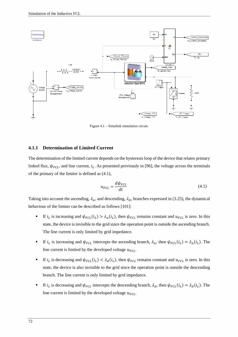
Simulation of the Inductive FCL
72
Figure 4.1 – Simulink simulation circuit.
4.1.1 Determination of Limited Current
The determination of the limited current depends on the hysteresis loop of the device that relates primary
linked flux, 𝜓𝐹𝐶𝐿, and line current, 𝑖𝐿. As presented previously in [96], the voltage across the terminals
of the primary of the limiter is defined as (4.1),
𝑢𝐹𝐶𝐿 =𝑑𝜓𝐹𝐶𝐿𝑑𝑡
(4.1)
Taking into account the ascending, 𝜆𝑎, and descending, 𝜆𝑑, branches expressed in (3.25), the dynamical
behaviour of the limiter can be described as follows [101]:
If 𝑖𝐿 is increasing and 𝜓𝐹𝐶𝐿(𝑖𝐿) > 𝜆𝑎(𝑖𝐿), then 𝜓𝐹𝐶𝐿 remains constant and 𝑢𝐹𝐶𝐿 is zero. In this
state, the device is invisible to the grid since the operation point is outside the ascending branch.
The line current is only limited by grid impedance.
If 𝑖𝐿 is increasing and 𝜓𝐹𝐶𝐿 intercepts the ascending branch, 𝜆𝑎, then 𝜓𝐹𝐶𝐿(𝑖𝐿) = 𝜆𝑎(𝑖𝐿). The
line current is limited by the developed voltage 𝑢𝐹𝐶𝐿.
If 𝑖𝐿 is decreasing and 𝜓𝐹𝐶𝐿(𝑖𝐿) < 𝜆𝑑(𝑖𝐿), then 𝜓𝐹𝐶𝐿 remains constant and 𝑢𝐹𝐶𝐿 is zero. In this
state, the device is also invisible to the grid since the operation point is outside the descending
branch. The line current is only limited by grid impedance.
If 𝑖𝐿 is decreasing and 𝜓𝐹𝐶𝐿 intercepts the descending branch, 𝜆𝑑, then 𝜓𝐹𝐶𝐿(𝑖𝐿) = 𝜆𝑑(𝑖𝐿). The
line current is limited by the developed voltage 𝑢𝐹𝐶𝐿.

Simulation of the Inductive FCL
73
4.1.1.1 Architecture of the Simulink Model
The architecture of the model, presented in Figure 4.2, is composed of three main blocks, whose
functions are:
Logic block: determines the operating point of the device according to the instant values of
primary linked flux and line current. This block provides an input to the current control block
specifying the operating point.
Limiting current determination block: selects the branch of the maximum hysteresis loop (𝜆𝑎 or
𝜆𝑑) to be related to 𝜓𝐹𝐶𝐿. In the case when |𝑖𝐿| > 𝐼𝑆𝐶, 𝜓0 is chosen instead of the maximum
branches. An input to the current control block is provided indicating the value of limited
current.
Current control block: depending on the input from the logic block, current can be limited by
the device or by grid impedance, according to the aforementioned algorithm. A controlled
current source is employed to limit, or not, the line current.
Figure 4.2 – Simulink FCL model architecture.
In this architecture, the line current is measured directly from the test grid by the native Current
Measurement block from Simulink while the primary linked flux is integrated from the voltage drop at
the terminals of the primary of the limiter, measured from the Voltage Measurement block from
Simulink. Current and linked flux are inputs for the logic and limiting current determination blocks.
4.1.1.2 Logic Block
The logic block, depicted in Figure 4.3, receives the primary linked flux and line current in order to
determine the operation point of the device according to the previously presented algorithm. Depending
on the operation point, a flag is used to specify such operating regime.

Simulation of the Inductive FCL
74
Figure 4.3 – Simulink logic block.
4.1.1.3 Limiting Current Determination Block
The limiting current determination block, whose architecture is presented in Figure 4.4, is based on the
same principle as nonlinear inductances [159]. The line current to be imposed in the grid is determined
from the linked flux by three lookup tables, corresponding to ascending, 𝜆𝑎, and descending, 𝜆𝑑,
branches as well as the iron core characteristic, 𝜓0. The chosen lookup table for current limitation is
dependent on current evolution (if is increasing or decreasing) and exceedance (or not) beyond 𝐼𝑆𝐶.
Figure 4.4 – Simulink limiting current determination block.

Simulation of the Inductive FCL
75
4.1.1.4 Current Control Block
The current control block, whose constituent elements are presented in Figure 4.5, is controllable by a
flag from the logic block that indicates the operating regime of the limiter. In the case of normal
operation, the terminals of the limiter are short-circuited making it transparent to the grid under this
regime. In fault condition, the current is imposed by a controlled current source that depends on the
determined limited current from the limiting current determination block.
Figure 4.5 – Simulink current control block.
4.1.2 Determination of Temperature
The determination of the temperature in each layer requires the knowledge of the induced current in the
superconducting tape. The induced current is modelled as a current source and is in series with six
resistors connected in parallel, as shown in Figure 4.6. These resistors represent the constituent layers
of the tape, i.e. copper (inner and outer), silver (inner and outer), Hastelloy and YBCO. Thus, the current
flowing in each layer is determined. This is implemented in Simulink. The contact resistance is omitted
from the model. Relevant variables in the figure are:
𝑖2: induced current in the superconducting ring.
𝑖𝐶𝑢(𝑖), 𝑖𝐶𝑢(𝑜), 𝑖𝐴𝑔(𝑖), 𝑖𝐴𝑔(𝑜), 𝑖𝐻𝑎𝑠𝑡, 𝑖𝑌𝐵𝐶𝑂: current in inner layer of copper, outer layer of copper,
inner layer of silver, outer layer of silver, Hastelloy and YBCO, respectively.

Simulation of the Inductive FCL
76
𝑅𝑒,𝐶𝑢(𝑖), 𝑅𝑒,𝐶𝑢(𝑜), 𝑅𝑒,𝐴𝑔(𝑖), 𝑅𝑒,𝐴𝑔(𝑜), 𝑅𝑒,𝐻𝑎𝑠𝑡, 𝑅𝑒,𝑌𝐵𝐶𝑂: electrical resistance of inner layer of
copper, outer layer of copper, inner layer of silver, outer layer of silver, Hastelloy and YBCO,
respectively.
Figure 4.6 – Equivalent circuit for determination of the current in each layer.
Knowing the current in each layer, a thermal-electrical analogy, formerly applied to resistive and air-coil
FCLs was adopted [88], [160]. The analogy, depicted in Figure 4.7, was implemented in Simulink.
Relevant variables in the figure are:
𝑅𝐶𝑜𝑛𝑣(𝑖), 𝑅𝐶𝑜𝑛𝑣(𝑜): resistances representing the convective heat exchange with liquid nitrogen
in inner and outer surfaces, respectively.
𝑅𝑡,𝐶𝑢(𝑖), 𝑅𝑡,𝐶𝑢(𝑜), 𝑅𝑡,𝐴𝑔(𝑖), 𝑅𝑡,𝐴𝑔(𝑜), 𝑅𝑡,𝐻𝑎𝑠𝑡, 𝑅𝑡,𝑌𝐵𝐶𝑂: resistances representing heat conduction
of inner layer of copper, outer layer of copper, inner layer of silver, outer layer of silver,
Hastelloy and YBCO, respectively.
𝑃𝐶𝑢(𝑖), 𝑃𝐶𝑢(𝑜), 𝑃𝐴𝑔(𝑖), 𝑃𝐴𝑔(𝑜), 𝑃𝐻𝑎𝑠𝑡, 𝑃𝑌𝐵𝐶𝑂: current source representing generated heat in inner
layer of copper, outer layer of copper, inner layer of silver, outer layer of silver, Hastelloy and
YBCO, respectively.
𝐶𝐶𝑢(𝑖), 𝐶𝐶𝑢(𝑜), 𝐶𝐴𝑔(𝑖), 𝐶𝐴𝑔(𝑜), 𝐶𝐻𝑎𝑠𝑡, 𝐶𝑌𝐵𝐶𝑂: capacitance representing the volumetric heat
capacity of inner layer of copper, outer layer of copper, inner layer of silver, outer layer of silver,
Hastelloy and YBCO, respectively.
𝑇𝐶𝑢(𝑖), 𝑇𝐶𝑢(𝑜), 𝑇𝐴𝑔(𝑖), 𝑇𝐴𝑔(𝑜), 𝑇𝐻𝑎𝑠𝑡, 𝑇𝑌𝐵𝐶𝑂: temperatures of inner layer of copper, outer layer of
copper, inner layer of silver, outer layer of silver, Hastelloy and YBCO, respectively.
Previous variables are governed by (2.6) to (2.9). Temperatures are determined by the voltage drop
between each point and the equivalent potential of the liquid nitrogen temperature, 𝑇𝐿𝑁2, corresponding
to 77.3.
AAAA AA
𝑅𝑒
,𝑌𝐵𝐶𝑂
𝑅𝑒
,𝐻𝑎𝑠𝑡
𝑅𝑒
,𝐶𝑢
(𝑜)
𝑅𝑒
,𝐶𝑢
(𝑖)
𝑅𝑒
,𝐴𝑔
(𝑜)
𝑅𝑒
,𝐴𝑔
(𝑖)
𝑖 𝐶𝑢
(𝑜)
𝑖 𝐶𝑢
(𝑖)
𝑖 𝐴𝑔
(𝑜)
𝑖 𝐴𝑔
(𝑖)
𝑖 𝑌𝐵𝐶𝑂
𝑖 𝐻𝑎𝑠𝑡
𝑖 2

Simulation of the Inductive FCL
77
Figure 4.7 – Thermal-electrical analogy for thermal behaviour prediction [88].
𝑅𝐶𝑜𝑛𝑣 (𝑖)
𝑅𝐶𝑜𝑛𝑣 (𝑜)
𝑃𝐶𝑢(𝑖)
𝑃𝐶𝑢(𝑜)
𝑃𝐴𝑔(𝑖)
𝑃𝐴𝑔(𝑜)
𝑃𝐻𝑎𝑠𝑡
𝑃𝑌𝐵𝐶𝑂
𝑇𝐶𝑢(𝑖)
𝑇𝐶𝑢(𝑜)
𝑇𝐴𝑔(𝑖)
𝑇𝐴𝑔(𝑜)
𝑇𝐻𝑎𝑠𝑡
𝑇𝑌𝐵𝐶𝑂
𝐶𝐶𝑢(𝑖)
𝐶𝐶𝑢(𝑜)
𝐶𝐴𝑔(𝑖)
𝐶𝐴𝑔(𝑜)
𝐶𝐻𝑎𝑠𝑡
𝐶𝑌𝐵𝐶𝑂
𝑅𝑡 ,𝐴𝑔(𝑖)
2
𝑅𝑡 ,𝐴𝑔(𝑖)
2
𝑅𝑡 ,𝐶𝑢(𝑖)
2
𝑅𝑡 ,𝐶𝑢(𝑖)
2
𝑅𝑡 ,𝐶𝑢(𝑜)
2
𝑅𝑡 ,𝐶𝑢(𝑜)
2
𝑅𝑡 ,𝐴𝑔(𝑜)
2
𝑅𝑡 ,𝐴𝑔(𝑜)
2
𝑅𝑡,𝐻𝑎𝑠𝑡2
𝑅𝑡,𝐻𝑎𝑠𝑡2
𝑅𝑡,𝑌𝐵𝐶𝑂2
𝑅𝑡,𝑌𝐵𝐶𝑂2
77.3 V

Simulation of the Inductive FCL
78
4.1.3 Solution Routine
The flow diagram of the reverse engineering methodology is illustrated in Figure 4.8. In each time step,
the dynamical electromagnetic state of the FCL is determined according to the maximum hysteresis loop
methodology and the thermal condition of the superconducting element is calculated by means of the
thermal-electrical analogy that provides the determination of the current in each layer of the
superconducting secondary.
In the first part of the routine, the limited current is calculated from the primary linked flux. After, the
current in the superconductor is determined based on the induced current from the primary
magnetomotive force. Knowing the current in the superconducting element, the temperature is computed
from the thermal-electrical analogy.
Figure 4.8 – Simultaneous electromagnetic and thermal computation flow diagram of the reverse engineering methodology.
Thick arrows represent the main process cycle. Thin arrows correspond to input and output of the allocated variables.
Compute next
time stepInitial conditions
definitionStart
?
Limitation by grid
impedanceYesNo
Determination of
current in the
secondary
Limitation by
maximum hysteresis
Thermal-electrical
analogy
Final time
step?End NoYes
tktk
tk
tk
tk-1 tk-1
Update parameters
tk
tk-1
𝑡𝑘 = 𝑡𝑘 1 + Δ𝑡
𝑡𝑘 𝑡𝑘
𝑡𝑘
𝑡𝑘
𝑡𝑘 1 𝑡𝑘 1
𝑡𝑘 1
𝑡𝑘 1
𝜓𝐹𝐶𝐿
𝑖1(𝜆𝑎 , 𝜆𝑑) 𝑖1(𝜓𝐹𝐶𝐿)
𝑖1
𝑖2 , 𝑖𝐶𝑢(𝑖), 𝑖𝐶𝑢(𝑜), 𝑖𝐴𝑔(𝑖)𝑖𝐴𝑔(𝑜), 𝑖𝐻𝑎𝑠𝑡 , 𝑖𝑌𝐵𝐶𝑂
𝑇𝐶𝑢(𝑖),𝑇𝐶𝑢(𝑜),𝑇𝐴𝑔(𝑖)𝑇𝐴𝑔(𝑜),𝑇𝐻𝑎𝑠𝑡 ,𝑇𝑌𝐵𝐶𝑂
𝑅𝑒 ,𝐶𝑢(𝑖),𝑅𝑒 ,𝐶𝑢(𝑜),𝑅𝑒 ,𝐴𝑔(𝑖)
𝑅𝑒 ,𝐴𝑔(𝑜),𝑅𝑒 ,𝐻𝑎𝑠𝑡 ,𝑅𝑒 ,𝑌𝐵𝐶𝑂
𝐶𝐶𝑢(𝑖),𝐶𝐶𝑢(𝑜),𝐶𝐴𝑔(𝑖),𝐶𝐴𝑔(𝑜),𝐶𝐻𝑎𝑠𝑡 ,𝐶𝑌𝐵𝐶𝑂𝑘𝐶𝑢(𝑖),𝑘𝐶𝑢(𝑜),𝑘𝐴𝑔(𝑖),𝑘𝐴𝑔(𝑜),𝑘𝐻𝑎𝑠𝑡 , 𝑘𝑌𝐵𝐶𝑂𝜌𝐶𝑢(𝑖),𝜌𝐶𝑢(𝑜),𝜌𝐴𝑔(𝑖),𝜌𝐴𝑔(𝑜),𝜌𝐻𝑎𝑠𝑡 ,𝜌𝑌𝐵𝐶𝑂
𝑅𝑡 ,𝐶𝑢(𝑖),𝑅𝑡 ,𝐶𝑢(𝑜),𝑅𝑡 ,𝐴𝑔(𝑖)𝑅𝑡 ,𝐴𝑔(𝑜),𝑅𝑡 ,𝐻𝑎𝑠𝑡 ,𝑅𝑡 ,𝑌𝐵𝐶𝑂
ℎ𝐶𝑜𝑛𝑣 (𝑖),ℎ𝐶𝑜𝑛𝑣 (𝑜)
𝑡𝑘
tk-1 tk-1
𝑡𝑘
𝑡𝑘 1 𝑡𝑘 1
𝜆𝑎 < 𝜓𝐹𝐶𝐿 < 𝜆𝑑

Simulation of the Inductive FCL
79
4.2 Simulation Results
The device is simulated in different scenarios concerning different conditions in the test grid, depicted
in Figure 4.9, namely the prospective short-circuit current controlled from the voltage source of the grid
operating at 50 Hz. The values for the considered scenarios are presented in Table 4.1. A total time
operation of 5 seconds is simulated. The load is short-circuited after 1 second of operation and cleared
2 seconds after this triggering.
Figure 4.9 – Simulation grid with the FCL in series with the line.
Table 4.1 – Simulated scenarios concerning different conditions in the grid.
Scenario Voltage source Line impedance Load resistance
1 73 Vrms
1.4 Ω 5.3 mH 300 Ω
2 83 Vrms
3 93 Vrms
4 103 Vrms
5 113 Vrms
4.2.1 Line Current
In the first peak after fault, as the short-circuit level of the grid increases the current limiting capacity,
defined as (4.2), decreases. This means that line current is not so effectively limited by the FCL in the
presence of high prospective line currents,
𝐼𝑙% =𝑖𝑝 𝑖𝑙
𝑖𝑝×100% (4.2)
where 𝑖𝑝 and 𝑖𝑙 are the prospective and limited current, respectively.
N1 = 60
HTS
𝑅𝐿𝑖𝑛𝑒 𝐿𝐿𝑖𝑛𝑒
𝑅𝐿𝑜𝑎𝑑 𝑢𝐺𝑟𝑖𝑑

Simulation of the Inductive FCL
80
From simulated scenarios, the best case of limiting capacity is 45.1% and the worst is 29.9%. The results
for all scenarios are presented in Table 4.2. After the first peak, these differences are minor but still
relevant, as observed in Figure 4.10.
Table 4.2 – Limiting capacity in the first peak after fault.
Scenario Prospective current Limited current (1st peak) Current limiting
capacity
1 47.5 A 26.1 A 45.1%
2 54.0 A 31.9 A 40.9%
3 60.5 A 38.6 A 36.2%
4 67.0 A 45.1 A 32.7%
5 73.5 A 51.5 A 29.9%
Figure 4.10 – Line current for different prospective line current scenarios.
4.2.2 Primary Linked Flux
The results of the primary linked flux are depicted in Figure 4.11. Comparing all scenarios, the amplitude
of the linked flux increases with the short-circuit level. However, differences are smaller between
scenarios with higher short-circuit levels, meaning that the limiter is becoming highly saturated for those

Simulation of the Inductive FCL
81
cases. A strong saturation means lower limiting capacity. In the first peak after the fault, the maximum
is 339 mWb for the case of scenario 1 and 423 mWb for scenario 5. In normal operation, the linked flux
presents an offset, but very small flux variation occurs meaning that the voltage drop over the primary
is negligible, as desired.
Figure 4.11 – Primary linked flux for different prospective line current scenarios.
4.2.3 Hysteresis Loop
As previously depicted, as the short-circuit current increase the primary linked flux also increase but
saturation effect is observed, in Figure 4.12. During normal operation, the linked flux does not vary in
time, remaining on a stable path, meaning that there is no voltage drop at the terminals of the limiter. In
fault condition, a large hysteresis loop emerges. The results of all scenarios are bounded by the
maximum loop.

Simulation of the Inductive FCL
82
Figure 4.12 – Hysteresis loop for different prospective line current scenarios.
4.2.4 Superconducting Current
The superconducting current for each scenario is presented in Figure 4.13. When the fault is triggered,
high peak currents between 3-4 times the critical current of the superconductor are observed. Major
differences among scenarios are observed in the first peak during fault regime. After the first peak, the
decay of amplitude for each scenario is very similar in all cases.
Figure 4.13 – Superconducting current for different prospective line current scenarios.

Simulation of the Inductive FCL
83
4.2.5 Temperature in Superconductor
For determination of the temperature in the superconductor, the presence of the holder is taken into
consideration. As for the primary, this holder provides mechanical support and ease of assembly in the
core. In return, reduced convection in the inner layer of the superconducting tape is expected. By
applying the thermal-electrical analogy, previously illustrated in Figure 4.7, it is considered that the
convection in inner layer is negligible, 𝑅𝐶𝑜𝑛𝑣(𝑖) → ∞, whilst convection in outer layer is modelled
by (3.20).
Because of high current peak values in the superconductor, the temperature in the inner layer of copper
presents a peak in the subsequent instants after the fault, reaching 88.8 K in the worst scenario. After
this transient regime, the temperature decreases to a stable path during fault operation. The temperature
in each layer of the superconducting ring is very similar to each other. A comparison, concerning
scenario 5, is made in Figure 4.14.
Figure 4.14 – Comparison between temperatures in each layer of the superconductor concerning simulation scenario 5.
Since minor differences in the temperature of each layer are observed, in order to compare all scenarios,
the temperature in the inner layer of copper is considered for presenting results. Furthermore, in the
validation presented in the next chapter, the temperature is measured on the surface of the inner layer of
the copper.
Simulation results, presented in Figure 4.15, show that the temperature reaches a peak in the early
moments after the short-circuit but decreases to a stable path afterwards, as presented in Figure 4.16. In
the first three cycles after the fault, a maximum temperature of 88.8 K is reached for the most severe
scenario and 86.6 K for the less severe scenario. After this transient, the temperate stabilises around

Simulation of the Inductive FCL
84
80.4 K and 79.9 K for the most severe and less severe scenarios, respectively. After the fault clearance,
the temperature returns to its original temperature.
Figure 4.15 – Temperature in superconductor for different prospective line current scenarios.
Figure 4.16 – Temperature in superconductor for different prospective line current scenarios.
Previous results considered the absence of convection in the inner surface of the superconducting ring
due to the presence of a holder. In the ideal case, if the holder is removed, convection is expected to
behave similarly either in outer and inner surfaces. In this case, convection in inner layer, 𝑅𝐶𝑜𝑛𝑣(𝑖), is
equivalent to convection in outer layer, 𝑅𝐶𝑜𝑛𝑣(𝑜). This is modelled by (3.20). A comparison, concerning
scenario 5, is presented in Figure 4.17. It can be seen that, as expected, the existence of convection in

Simulation of the Inductive FCL
85
the inner layer improves the thermal behaviour by reducing temperature during normal and short-circuit
operation. Besides a lower temperature peak, the stable path of temperature during steady-state of fault
is also lower, as depicted in Figure 4.18.
Figure 4.17 – Convection dependence of the temperature in superconductor concerning scenario 5.
Figure 4.18 – Convection dependence of the temperature in superconductor concerning simulation scenario 5.

Simulation of the Inductive FCL
86
4.3 Summary
In this chapter, the simulation methodology and solution routine, implemented in Simulink, from
Matlab, used to predict the dynamical electromagnetic-thermal behaviour of the limiter in electrical
grids have been presented.
The methodology for the prediction of the electromagnetic behaviour of the limiter considered a reverse
engineering methodology based on the maximum hysteresis loop of the device, presented in the previous
chapter. On the other hand, a thermal-electrical analogy, also presented in the previous chapter, has been
used for the determination of the temperature in each layer of the superconducting tape composing the
limiter.
The developed simulation tool, fully compatible with Simscape Power Systems toolbox, from Simulink,
provides simulation results in few minutes. Five scenarios, with different prospective line currents, have
been simulated. A total simulation time of 5 seconds, with a long-term fault of 2 seconds, has been
considered. Simulated line current, primary linked flux, current in HTS tape and temperature in each
layer of the tape have been presented. Computation time of each scenario took less than 5 minutes. In
the less severe simulation scenario (prospective current of 47.5 A), line current was limited to 26.1 A in
the first peak after fault, meaning a limiting capacity of 45.1%. Concerning the most severe scenario
(prospective current of 73.5 A), the current in the first peak after fault was limited to 51.5 A, meaning
29.9% of current limiting capacity. Simulation results of the limiter operating at fault condition, for the
five different scenarios, are summarised in Table 4.3.
Table 4.3 – Summary of simulation results of the limiter subjected to a different prospective line current scenarios.
Scenario Prospective
current
Limited
current
(1st peak)
Current
limiting
capacity
Linked flux
(1st peak)
Superconducting
current
(1st peak)
Peak
temperature
1 47.5 A 26.1 A 45.1% 0.339 Wb 383.5 A 86.6 K
2 54.0 A 31.9 A 40.9% 0.364 Wb 390.5 A 87.3 K
3 60.5 A 38.6 A 36.2% 0.385 Wb 392.5 A 87.6 K
4 67.0 A 45.1 A 32.7% 0.404 Wb 398.0 A 88.2 K
5 73.5 A 51.5 A 29.9% 0.423 Wb 403.3 A 88.8 K

Experimental Validation of Models
87
5 Experimental Validation of Models
In order to validate the models, a prototype was subjected to short-circuit tests. Different short-circuit
levels were considered. During the tests, several values were measured and registered, namely the grid
voltage, the line current, the primary linked flux, as well as the current in the superconductor and its
temperature.
5.1 Experimental Details
The developed prototype is shown in Figure 5.1. The prototype was installed in a test grid, as depicted
in Figure 5.2. The grid is composed of a controllable voltage source, a line impedance8 and a load
resistance. The primary is connected in series with the grid under protection and the superconducting
secondary is cooled in an open bath of liquid nitrogen. Faults were applied in the grid by short-circuiting
the load through a circuit-breaker. The electrical parameters of the grid are presented in Table 5.1.
Figure 5.1 – Developed prototype for validation of models.
8 In addition to the test resistance of 1.4 Ω, the resistance of the connection lines (0.2 Ω) were also considered.
Magnetic
corePrimary
Secondary
(inside cryostat)
5

Experimental Validation of Models
88
Figure 5.2 – Test grid with the FCL in series with the line.
Table 5.1 – Electrical parameters of the test grid.
Parameters Value
Voltage source 49 – 113 Vrms
Frequency 50 Hz
Line inductance 5.3 mH
Line resistance 1.6 Ω
Load resistance 300 Ω
5.1.1 Experimental Apparatus
The experimental test bench is schematically depicted in Figure 5.3. The following elements have been
used:
Auto-transformer: Allows to apply up to 400 V in the primary of the galvanic isolation
transformer.
Isolation transformer: A 2 kVA transformer, providing galvanic separation between the power
grid and test grid.
Line: An air-core copper coil with a resistance of 1.4 Ω and inductance of 5.3 mH. An additional
resistance, introduced by the connection cables, is measured and taken into account for
simulation purposes.
Load: A 300 Ω resistor.
Breaker: Inserted in parallel to the load, in order to intentionally introduce faults by
short-circuiting the load.
N1 = 60
1.6 Ω
HTS
5.3 mH
300 Ω 𝑢𝐺𝑟𝑖𝑑

Experimental Validation of Models
89
Fault Current Limiter: The prototype under study with the aforementioned constitutive parts
(magnetic core, primary, superconducting secondary and cryostat).
Auxiliary winding with integrator: Sensing device to measure the primary linked flux. The
auxiliary winding is wound around the core and its voltage drop is integrated.
Silicon diode: Temperature sensor, with reference DT-670 from Lakeshore. The diode is biased
with a 10 µA DC current source.
Rogowski coil with integrator and amplifier: Sensor to measure the current in the secondary.
The coil is wound around the superconductor and the voltage is integrated and amplified.
Hall probe: Hall effect current probe, with reference A622 from Tektronix, to measure the line
current.
Data acquisition board: Universal serial bus (USB) data logger (National Instruments-6008) to
read the voltage of a hall probe sensing the line current (Tektronix A622), the voltage image of
the primary linked flux, and the voltage proportional to the current in the superconducting ring.
Digital multimeter: Data logger (Keithley-2001) over the standard 488 of the Institute of
Electrical and Electronics Engineers (IEEE), generally known as IEEE-488, used to read the
voltage of the silicon diode proportional to the surface temperature of the superconducting ring.
Computer: Running a Matlab routine for data logging from USB and IEEE-488 interfaces. The
sampling rate of the National Instruments-6008 acquisition board, via USB, is 2500 samples per
second and 24 samples per second for the case of the Keithley-2001, via IEEE-488.
Figure 5.3 – Schematic diagram of the test bench. The auxiliary winding, represented in the same limb of the superconducting
ring for diagram simplification, is wound around the primary to consider the leakage reactance.
The real apparatus is shown in Figure 5.4 and Figure 5.5.
Integrator
Line
Auto-Transformer
0 – 400 VrmsIsolation transformer
380 Vrms / 133 Vrms FCL
Grid
vo
ltage
Load
10 µA
V
V V
VV
V
Hall probe
Rogowski coil with
integrator
Silicon diode
HTS ring
Auxiliary winding
Primary winding

Experimental Validation of Models
90
Figure 5.4 – Laboratory apparatus during experiments.
(a) (b) Figure 5.5 – Experimental details of the temperature and current sensors. The cryostat, Celeron holder and a part of the iron
core are also shown. (a) Diagram. (b) Real apparatus.
Since the analogue inputs of the National Instruments-6008 are limited to ±10 V, signal conditioning is
required in order to measure higher voltages. Thus, a differential amplifier, as depicted in Figure 5.6,
was used. A single supply quad operational amplifier MC3403 was employed. Supply voltage for the
operational amplifier is provided from an adjustable power supply with reference PS23023 from Kiotto
Company. The supply was defined as ±10 V. The output of the differential amplifier is given by (5.2),
NI-6008
Limiter
Auto-transformer
Isolation transformer
Keithley-2001
Hall probe
Line coil (behind the limiter)
Load
Power supply

Experimental Validation of Models
91
𝑣𝑜 = 𝑣1 ∙ (𝑅2𝑅1) + 𝑣2 ∙ (
𝑅4𝑅3 + 𝑅4
) ∙ (𝑅1 + 𝑅2𝑅1
) (5.1)
where 𝑣0 is the output voltage, 𝑣1 and 𝑣2 are the input terminals, and 𝑅1, 𝑅2, 𝑅3 and 𝑅4 are resistances
for signal conditioning. When 𝑅1 = 𝑅3 and 𝑅2 = 𝑅4 the output can be simplified to (5.2),
𝑣𝑜 =𝑅2𝑅1∙ (𝑣2 𝑣1) (5.2)
Figure 5.6 – Differential amplifier for signal conditioning of voltage measurements.
Considering (5.2), the gain of the differential amplifier, defined as the relation 𝑅2/𝑅1, for each
conditioned measured quantity is presented in Table 5.2. After data acquisition, an inverse gain is
applied by software.
Table 5.2 – Electrical parameters of the signal conditioning.
Analog input Measured voltage 𝑅1 𝑅2 𝑅3 𝑅4 Gain
1 Line impedance 10 kΩ 1 kΩ 10 kΩ 1 kΩ 0.1
3 Linked flux sensor coil9 22 kΩ 22 kΩ 22 kΩ 22 kΩ 1
The gain of the channel of the line current, measured with the Tektronix A622 current probe, is
100 mV/A, directly adapted from the measuring device. In the case of the Rogowski coil, the gain is
16 mV/A with no need for additional signal conditioning. Concerning data logging from digital
multimeter Keithley-2001, there is no need for electronic signal conditioning since its voltage operating
range is adequate for the voltage output range of the silicon diode.
9 The signal conditioning gain is 1 but due to the turn number relation between the primary winding (60 turns) and
sensor winding (70 turns), the final gain is the relation 60/70, corresponding to 0.857.
+
-𝑣1
𝑣2 𝑣𝑜
𝑅1
𝑅2
𝑅3 𝑅4
MC 3403

Experimental Validation of Models
92
Due to the need of using two distinct data loggers operating at the same time with different interfaces,
data acquisition is managed by means of a GUI in Matlab. This GUI, presented in Figure 5.7, allows
logging measurements from data acquisition board and digital multimeter in parallel real time. Up to
eight analogue input channels of the National Instruments-6008 in reference single ended mode and one
differential input of the Keithley-2001 can be logged. Several definitions of data acquisition are
available, such as sampling rate, voltage range, channel names, gains and resolution. After data
recording, results can be observed directly in the GUI and a spreadsheet is generated with a defined
filename.
Figure 5.7 – Developed GUI for data logging from the data acquisition board National Instruments-6008 and digital multimeter
Keithley-2001.
5.1.2 Rogowski Coil
A Rogowski coil, shown in Figure 5.8, specially adapted for the reduced dimensions of the coated
conductor and a corresponding signal integrator were developed and calibrated. This coil is open-ended
and flexible, allowing it to be wound around the superconducting tape. The measured values were
acquired by the National Instruments data acquisition board. Line current and linked flux were also
measured with this acquisition board.
An integrator and active amplifier with a gain of 16 mV/A was used for reading the output voltages of
the Rogowski coil that are images of the current in the superconducting ring. It is taken into account that
the output voltages are with 90º of phase shift with respect to current.

Experimental Validation of Models
93
Figure 5.8 – Rogoswski coil with superconducting tape inserted.
5.1.3 DT-670 Silicon Diode
Measuring temperature in the superconducting tape can be performed by silicon diodes that are sensible
to temperature. This solution has been used in several works, see e.g. [161]–[163]. In this work, a silicon
diode sensor with reference DT-670 from Lakeshore [164] was used for temperature measurement on
the surface of the coated conductor according to its standard calibration curve [165]. The surface of the
temperature sensor was greased with Apiezon N and enclosed by Teflon tape between the Celeron holder
and the superconducting tape, applied as shown in Figure 5.5. Voltage signals proportional to
temperature were acquired with the Keithley-2001 and logged with the developed GUI from the
IEEE-488 interface. The configurations of the Keithley-2001 are very important for sample rating. The
most important configuration parameters for data acquisition over IEEE-488 bus are:
Aperture (APER): It is the integration time of the analogue/digital converter, i.e. the period of
time that the input signal is measured (166.67×10⁻⁶ to 200×10-3 seconds). The integration time
has influence in the resolution, reading noise as well as the sampling rate.
Number of Power Line Cycles (NPLC): This parameter is also related to the integration time,
corresponding to the number of power line cycles (0.01 to 10) that the input signal is measured.
Despite leading to increased noise and lower resolution, a lower NPLC provides faster readings
than a higher NPLC. Since APER and NPLC represent both the integration time, when setting
NPLC, the aperture value is updated accordingly to the value of NPLC. If NPLC is not set, the
defined value of APER is considered for the integration time.
Digits (DIG): Measurement resolution (4 to 9 digits). Few digits for speed, many digits for
high-resolution.
Filter: Used to stabilise noisy measurements. Analog and digital filters are available. The
analogue filter is a simple RC circuit. On the other side, two types of digital filters are available:
averaging and advanced. The former is based on an average of readings inside a specified range

Experimental Validation of Models
94
while the latter performs a dynamic average of reading considering readings inside and outside
the specified range.
Range: Measurement range (-1.1×10³ to 1.1×10³ V). Affects resolution and accuracy.
These values, considering a trade-off between precision and speed, are presented in Table 5.3.
Table 5.3 – Configuration parameters for Keithley-2001 data acquisition over IEEE-488 bus.
Parameter Value
APER 166.67×10⁻⁶ seconds
NPLC10 0.01 cycles
DIG 5 digits
Filter Disabled
Range 1.04 – 0.98 V
The diode is connected to digital multimeter in a two-wire configuration for voltage measurement, as
illustrated in Figure 5.9.
Figure 5.9 – Silicon diode connection to digital multimeter in two-wire configuration. Adapted from [166].
The silicon diode requires a stable 10 µA DC current source. This current source was built as shown in
Figure 5.10, in which the load is the diode. Supply voltage of ±10 V to the OP 27 operational amplifier
is provided from an adjustable power supply with reference PS23023 from Kiotto Company. Reference
voltage, 𝑈𝑅𝑒𝑓, is provided from a power source ALR3003 from ELC Company. The parameters of
reference voltage and resistance of current adjusting are presented in Table 5.4.
10 If NPLC is not set, the defined value of APER is considered for the integration time of the analogue/digital
converter. Otherwise, if NPLC is set, the APER parameter is not considered.
Keithley Model 2001
Sil
ico
n d
iod
e
Cu
rren
t so
urc
e
(10
µA
)

Experimental Validation of Models
95
Figure 5.10 – Precision 10 µA current source.
Table 5.4 – Parameters for precision 10 µA current source.
Parameter Value
𝑈𝑅𝑒𝑓 4.99 V
𝑅1 499 kΩ
From the standard curve of the diode [165], presented in Figure 5.11, the temperature measured, 𝑇𝐷, in
the range 75 – 95 K can be approximated by (5.3),
𝑇𝐷 =1.165 𝑣𝐷0.001773
(5.3)
where 𝑣𝐷 is the voltage drop at the terminals of the diode.
Figure 5.11 – Temperature response curve of the DT-670 silicon diode in the range 75 – 95 K.Adapted from [165]
+
-OP 27
Load
𝑅1 𝑈𝑅𝑒𝑓 𝑈𝑅𝑒𝑓
𝑅1
0.98
0.99
1.00
1.01
1.02
1.03
1.04
75 80 85 90 95
Volt
age
(V)
Temperature (K)

Experimental Validation of Models
96
5.2 Comparison Between Simulations and Experimental Results
A total time operation of 5 seconds was considered. Using a quad-core 2.83 GHz processor, 8 GB RAM
computer, the simulation of this problem took less than 5 minutes. In order to quantify divergences
between simulated and experimental results, the percentage error, 𝐸%, defined in (5.4), is used,
𝐸% = |𝑥𝐸𝑥𝑝 𝑥𝑆𝑖𝑚
𝑥𝐸𝑥𝑝| ×100% (5.4)
where 𝑥𝐸𝑥𝑝 and 𝑥𝑆𝑖𝑚 are experimental and simulated quantities, respectively.
5.2.1 Line Current
The results of the line current are presented and compared in Figure 5.12. The maximum prospective
line current of 30.1 A was limited to 18.4 A in the first peak during fault operation in the simulated case
and 18.9 A in the experimental case. During this first cycle, the error is 2.6% in the positive peak and
1.0% in the negative peak. After the first cycle in fault operation, the line current amplitude sets around
11.9 A, for both simulation and experimental cases, with a very reduced error.
Figure 5.12 – Comparison between simulation and experimental results of the line current.
5.2.2 Primary Linked Flux
The primary linked flux as a function of time is depicted in Figure 5.13. Similarly to results of line
current, the major difference occurs during the first peak after the fault, in which the maximum
amplitudes are 292 mWb and 242 mWb for the simulated and experimental cases, respectively,

Experimental Validation of Models
97
corresponding to an error of 20.7%. The error is reduced to 12.3% (simulated value of 200 mWb and
experimental value of 228 mWb) and 5.5% (simulated value of 230 mWb and experimental value of
218 mW) in second and third peaks, respectively. In the following cycles during fault condition, the
maximum experimental flux amplitude sets around 210 mWb for both simulation and experimental
cases. A small phase shift between measurements and simulations is observed.
Figure 5.13 – Comparison between simulation and experimental results of the primary linked flux.
5.2.3 Hysteresis Loop
The excursion of the hysteresis loop from a transition between the fault operation and normal operation
is depicted in Figure 5.14. The shape of the experimental loop is in agreement with simulations. The
wider path cycles observed in the experimental results correspond to the initial cycles after the fault
triggering. After the initial cycles, minor differences are observed. This behaviour suggests that the
parameter 𝐼𝐻𝑇𝑆∗ of the methodology based on the maximum hysteresis loop can be dynamic.

Experimental Validation of Models
98
Figure 5.14 – Comparison between simulation and experimental results of the hysteresis loop.
5.2.4 Superconducting Current
The current in the superconductor is shown in Figure 5.15. The measured peak current, during fault
condition, reached three times the critical current but decreased to nearly its critical value during this
regime. This is an important remark for thermal stability. Comparing experimental results to
simulations, despite some differences in the first two periods after fault, results are in great accordance.
The major difference between simulation and experimental results occurs in the first peak after fault,
corresponding to an error of 15.7% (simulated value of 357.5 A and experimental value of 308.9 A). In
the next peaks, the error is reduced to 3.7%, 11.3% and 1.8% for second, third and fourth peaks,
respectively. In the following cycles, results are in great accordance. For prospective line currents higher
than 40 A, the experimental results of the superconducting current show a non-sinusoidal behaviour.
This means that the simple model for the determination of the induced current as a function of primary
magnetomotive force correctly determines the amplitude of the current but non-sinusoidal phenomenon,
arising from high current values, is not properly represented. Nevertheless, in the case of smaller
amplitudes, the non-sinusoidal behaviour is not so evident whereby the shape of the simulated results is
closer to the experimental results, as presented in Appendix D. Since these simulation results are used
as input for the determination of the temperature in the superconducting tape, it is important to
understand their relevance. This task is performed following.

Experimental Validation of Models
99
Figure 5.15 – Comparison between simulation and experimental results of the superconducting current.
5.2.5 Temperature in Superconductor
The temperature in the superconductor is represented in Figure 5.16. Experimental results show a peak
of about 85.5 K in the early moments after the short-circuit but decrease, in about 0.5 seconds, to a stable
path around 80 K. This means that safe operation is achieved from the thermal stability point of view.
When the fault is cleared, the recovery of the initial temperature takes about 0.6 – 0.8 seconds.
At normal regime operation, a small difference in temperature between simulation and experimental
results are observed. Whilst the experimental results give 77.4 K, the simulation results estimate 77.7 K.
This means an error of 0.4%. In fault condition, the simulated peak temperature is 86.0 K, representing
an error of 0.6% with respect to experimental measurements. During fault operation, good agreement
between experiments and simulations are observed. However, due to discrete measurements, the true
peak may not have been computationally acquired, but a point near instead. This constraint is explained
from the reduced sampling rate of the digital multimeter over IEEE-488 bus interface due to high
precision measurement needs. A small shift is also observed which is due to the thermal inertia of the
sensor.
Despite not having relevance unless a fault occurs at that moment, the most significant difference
between simulation and experimental results occurs in the following moments after the fault clearance.
Besides the thermal inertia of the sensor, this can be explained by a hysteretic behaviour of the
convection. From the literature, it is suggested that the heat transfer coefficient, when cooling from high
temperatures, the boiling regions may be hysteretically extended down [86], [167]. The presence of
Teflon tape around the superconducting tape also contributes for a slower heat removal.

Experimental Validation of Models
100
Figure 5.16 – Comparison between simulation and experimental results of the temperature in the tape.
5.3 Summary
In this chapter, the experimental details of the implemented prototype and sensors for data acquisition
have been presented. The prototype has been inserted in a test electrical grid and subjected to several
short-circuit faults with prospective currents from 30.1 A to 69.2 A. Line current, primary linked flux,
current in superconducting secondary as well as temperature in the surface of the superconducting
secondary have been measured. A commercial Hall probe and silicon diode have been used to measure
line current and temperature on the surface of the superconductor, respectively. On the other hand, an
auxiliary winding for measuring the primary linked flux and a Rogowski coil for the measurement of
the current in superconductor have been prototyped. The temperature on the surface of the
superconductor was acquired with a high precision digital multimeter whilst the other quantities were
acquired by a data acquisition board. All these quantities have been compared to simulations. Good
agreement was achieved. Results of the peak values of the limiter operating at fault condition, for a
prospective line current of 30.1 A, in simulation and experimental cases, are summarised in Table 5.5.
More results can be found in Appendix D.

Experimental Validation of Models
101
Table 5.5 – Summary of experimental and simulation results of the limiter subjected to a prospective line current of 30.1 A.
Scenario
Limited
current
amplitude
Linked flux
amplitude
Superconducting
current
amplitude
Temperature
Value Error Value Error Value Error Value Error
Steady state
(normal)
Simulation 0.3 A
0.0%
<0.005 Wb
0.0%
18.0 A
4.3%
77.7 K
0.4%
Experimental 0.3 A <0.005 Wb 18.8 A 77.4 K
1st peak
(fault)
Simulation 18.4 A
2.6%
0.292 Wb
20.7%
357.5 A
15.7%
86.0 K
0.6%
Experimental 18.9 A 0.242 Wb 308.9 A 85.5 K
2nd peak
(fault)
Simulation 10.2 A
1.0%
0.200 Wb
12.3%
305.2 A
3.7%
-
-
Experimental 10.3 A 0.228 Wb 316.9 A -
3rd peak
(fault)
Simulation 12.5 A
5.0%
0.230 Wb
5.5%
297.7 A
11.3%
-
-
Experimental 11.9 A 0.218 Wb 267.5 A -
4th peak
(fault)
Simulation 11.7 A
5.4%
0.222 Wb
7.1%
279.8 A
1.8%
-
-
Experimental 11.1 A 0.239 Wb 274.9 A -
5th peak
(fault)
Simulation 12.0 A
5.3%
0.224 Wb
5.7%
266.9 A
0.1%
-
-
Experimental 11.4 A 0.212 Wb 267.1 A -
6th peak
(fault)
Simulation 11.9 A
2.6%
0.224 Wb
6.3%
254.3 A
4.4%
-
-
Experimental 11.6 A 0.239 Wb 266.1 A -

Experimental Validation of Models
102

Conclusions
103
6 Conclusions
In this work, a contribution for the development of inductive type superconducting fault current limiters
has been made by providing experimental details and models that might be included in the design of
such type of limiters operating in electrical power grids. The influence of the constitutive parts
composing the limiter has been studied in order to design, model and simulate such type of limiter.
The research question of this work, presented in Chapter 1, aims to identify how the properties of the
constitutive parts of the inductive type FCL can be considered to model, simulate and design such
limiter. In this work, an electromagnetic-thermal analysis of the constitutive parts composing the FCL
has been carried out, namely: primary winding, superconducting secondary, magnetic core and cryostat
with liquid nitrogen. The behaviour of the magnetic linkage between primary and superconducting
secondary during normal and fault operation has been studied. Thermal dependent properties of the
superconductor have been taken into account, namely: critical current density, 𝑛-value, resistivity,
thermal conductivity, heat capacity and convection. A laboratory-scale prototype has been built and
experimental data have been acquired in order to validate previous models based on electromagnetic
and thermal phenomena. A simulation tool, providing fast simulations of the electromagnetic-thermal
behaviour of the inductive limiter operating in a grid, has been proposed.
Regarding the hypothesis, also presented in Chapter 1, a relationship between the independent variable
(simulation methodology) and dependent variable (simulation results compared to real experimental
results) can be reached. The developed simulation tool, implemented in Simulink, provide simulation
results of the limiter operating in electrical grids with reasonable agreement to experimental results.
Furthermore, with the use of this tool, fast simulations, in the order of few minutes (less than 5 minutes),
can be performed. This is particularly important, since simulations of FCLs in electrical grids generally
require time-consuming computation, as e.g. FEM simulations [72], [79].
6.1 Summary and Discussion
The performed activities of this work are presented and discussed following:
Design of an inductive type FCL composed of a two-legged closed magnetic core wound by a
primary winding, made by copper wire, and a short-circuited superconducting secondary, made
6

Conclusions
104
by SuperPower SCS4050 tape. The latter is supported by a Celeron holder and housed inside a
cryostat with liquid nitrogen. Related tasks:
o Design of an acrylic holder to support the primary winding and ease the assembly in the
limiter. Copper with a cross section of 1.5 mm2 was chosen due to ease of winding
manufacturing and low price. An auxiliary winding, separated from the primary, was
also wound around the acrylic holder. This auxiliary winding, also made by copper, is
used to measure the linked flux with the primary.
o Design of a cryostat wounding a leg of the magnetic core. This cryostat, made by
extruded polystyrene, was designed focusing an easy assembly for experimental
measurements. It can store about 0.25 L of liquid nitrogen.
o Development of a holder to perform joints of superconducting tapes in the form of rings.
This holder, adapted to support heating and cooling cycles, was made from
stainless-steel in a CNC machine. With this holder, both terminals of superconducting
tape are soldered with Sn96.5-Ag3.5 paste, performing rings with 40 mm radius. Prior
to soldering, copper overlayers of the tape (on the joint regions) have been removed by
chemical etching. This procedure requires to deep the tape inside etchant for at least
20 minutes in order to completely remove copper layers, as observed by scanning
electron microscopies and energy disruptive x-ray spectroscopies.
o Design of a Celeron holder to support superconducting rings. Presenting low thermal
expansion, Celeron is a suitable material to be housed inside the cryostat. Besides, it
also allowed to use a Rogowski coil wounding the superconducting ring.
Development of a fast simulation tool, in Simulink/Matlab, for the prediction of the
electromagnetic-thermal behaviour of the designed limiter operating in a grid. Several
short-circuits with different prospective line currents have been simulated. In the less severe
scenario presented (prospective current of 47.5 A), the current limiting capacity was 45.1%
whilst in the most severe scenario (prospective current of 73.5 A), the current limiting capacity
was 29.9%. Temperatures in superconducting tapes range from 86.6 K (less severe scenario) to
88.8 K (most severe scenario). Related tasks:
o Experimental characterisation of critical current density and n-index of the commercial
SuperPower SCS4050 superconducting tape. Four points method technique, according
to IEC 61788-3, has been performed. At 77.3 K, self-field, the sample subjected to
measurement presented an engineering current density of 255.8 A·mm-2 and n-value of
31.71.
o Modelling (based on literature) of the temperature dependence of critical current density
and n-index of YBCO as well as the temperature dependence of electrical resistivity,

Conclusions
105
heat capacity and thermal conductivity of each layer composing the superconducting
tape, i.e., copper, silver, Hastelloy and YBCO. The convective heat transfer between
the surface of the superconducting tape and liquid nitrogen has also been modelled.
These properties are applied in a thermal-electrical analogy used to predict the thermal
behaviour of each layer of the superconducting tape.
o Development of an electromagnetic model describing the dynamical behaviour of the
induced currents in superconducting secondary of the limiter. This model is based on
the empirical knowledge of the induced currents in superconducting ring as a function
of the primary magnetomotive force and time after the beginning of short circuit fault.
The determined values are used as input in the thermal-electrical analogy. The model
correctly determines the current in superconductor for low amplitudes of prospective
currents (up to about 40 A). However, for higher prospective line currents, the measured
induced currents in superconducting ring present a non-sinusoidal behaviour that is not
predicted in simulations. This leads to further investigations regarding such
non-sinusoidal behaviour.
o Experimental characterisation of the device according to the maximum hysteresis loop
methodology, namely measurement of the relation between primary linked flux and
current in the absence of the superconducting secondary as well as measurement of the
maximum induced current in superconductor for which current limitation is not
performed. The value of this maximum induced current, measured with a Rogowski
coil, was 182 A.
Experimental assessment of a developed prototype (based on the performed design) and
validation of simulation methodologies. In order to gather experimental results, the prototype is
inserted in a test electrical grid subjected to fault occurrences, allowing to measure line current,
primary linked flux, current in superconductor and temperature on the surface of
superconductor. The prototype has been subjected to short-circuit faults with prospective line
currents from 30.1 A to 69.2 A (in the main body of the text, results concerning a prospective
line current of 30.1 A are presented and discussed whilst other scenarios are presented in
Appendix D). The results provided by the maximum hysteresis loop methodology, namely
primary line current and linked flux, have been compared to experimental results. These results
are in good accordance meaning that the methodology is suitable for the prediction of the
electromagnetic behaviour of the limiter. On the other hand, the thermal-electrical methodology
correctly determines the amplitude of the current in superconducting ring. However, for
prospective line currents higher than 40 A, non-sinusoidal behaviour of the induced currents in
superconductor is experimentally observed. The modelling of this behaviour must be
investigated in future works since the simulation model correctly predicts the amplitude values

Conclusions
106
but not the non-sinusoidal behaviour. Concerning the temperature prediction, the
thermal-electrical methodology present simulation results in good accordance to experimental
measurements (for instance, in the case of a prospective line current of 30.1 A, simulation results
of peak temperature gave 86.0 K whilst measured results gave 85.5 K, meaning a relative error
of 0.4%). The greatest differences are observed during fault clearance, whereby this should be
investigated in future works in order to fully validate the methodology. These measurements
have been performed by using several equipment. Related tasks:
o Measurement of line current with a commercial Tektronix A622 Hall probe sensor.
Measurement of linked flux with a prototyped auxiliary coil (wounding the magnetic
core). Measurement of superconducting current with a prototyped Rogowski coil
(wounding the superconducting ring) specially built to be inserted inside the cryostat.
Measurement of temperature in the surface of superconducting tape with a commercial
Lakeshore DT-670 silicon diode.
o Development of a graphical user interface for laboratory measurements with data
acquisition board NI-6008 (over USB interface) and digital multimeter Keithley-2001
(over IEEE-488 interface) operating simultaneously. With this graphical interface, it is
possible to start and stop data logging, from both USB and IEEE-488 interfaces, at the
same timestamp. The properties and acquired results of these data loggers can be
managed, saved and observed directly from the graphical interface. Line current, linked
flux and superconducting current have been measured with NI-6008 whilst temperature
in the surface of superconducting tape has been measured with Keithley-2001.
6.2 Future Work
The following aspects are recommended to be considered for future work:
The parameter 𝐼𝐻𝑇𝑆∗ of the electromagnetic methodology based on the maximum hysteresis loop
of the limiter should be considered dynamic in order to simulate the hysteresis loop more
realistically, especially in the initial transient after a fault.
The amplitude decay of the current in the superconducting ring as a function of short-circuit
time must be devoted to further investigations. A theoretical model based on the dimensions
and properties of the superconducting tape should be able to determine peak amplitude and
decay as a function of time, when a short-circuit is occurring in the inductive limiter. This will
avoid the need for experimental assessment for characterisation of secondary superconducting
rings, during the design stage of a limiter.
The equivalent circuit model to determine the current in each layer of the tape does not take into
account the contact resistance of the soldered joint of the superconducting ring. Further studies

Conclusions
107
must be devoted in order to assess the influence of the contact resistance of the joint region in
quench phenomenona.
The fast method to determine the induced currents in the superconducting ring should be further
investigated in order to better predict the non-sinusoidal behaviour of these currents observed
experimentally.
Study of the temperature decay in the superconducting ring after a fault clearance. The hysteretic
behaviour of convective heat transfer coefficient should be clarified. The influence of auxiliary
materials, such as Teflon, in the cooling process, should also be studied.
Study of prototypes at higher power ratings and validation of simulation methodologies at such
power ratings.

Conclusions
108

References
109
References
[1] M. Noe and M. Steurer, ‘High-Temperature Superconductor Fault Current Limiters: Concepts,
Applications, and Development Status’, Superconductor Science and Technology, vol. 20, no. 3,
pp. R15–R29, Mar. 2007.
[2] W. Yuan, ‘Second-Generation High-Temperature Superconducting Coils and Their Applications
for Energy Storage’, Springer London, London, 2010.
[3] V. Akhmatov, ‘Analysis of Dynamic Behaviour of Electric Power Systems With Large Amount
of Wind Power’, PhD Thesis, Technical University of Denmark, 2003.
[4] R. Dommerque, S. Krämer, A. Hobl, R. Böhm, M. Bludau, J. Bock, D. Klaus, H. Piereder, A.
Wilson, T. Krüger, G. Pfeiffer, K. Pfeiffer, and S. Elschner, ‘First Commercial Medium Voltage
Superconducting Fault-Current Limiters: Production, Test and Installation’, Superconductor
Science and Technology, vol. 23, no. 3, p. 34020, Mar. 2010.
[5] S. Stavrev, ‘Modelling of High Temperature Superconductors for AC Power Applications’, PhD
Thesis, École Polytechnique Fédérale de Lausanne, 2002.
[6] K. Bauml and U. Kaltenborn, ‘Inductive Shielded Superconducting Fault Current Limiter - A
New Cost Effective Solution For Industrial Network Applications’, Petroleum and Chemical
Industry Conference Europe Conference Proceedings (PCIC EUROPE), 2011.
[7] V. Sokolovsky, V. Meerovich, G. Grader, and G. Shter, ‘Experimental Investigation of Current-
Limiting Device Model Based on High-Tc Superconductors’, Physica C: Superconductivity, vol.
209, pp. 277–280, Apr. 1993.
[8] I. Vajda, A. Gyore, A. Szalay, V. Sokolovsky, and W. Gawalek, ‘Improved Design and System
Approach of a Three Phase Inductive HTS Fault Current Limiter for a 12 kVA Synchronous
Generator’, IEEE Transactions on Applied Superconductivity, vol. 13, no. 2, pp. 2000–2003, Jun.
2003.
[9] N. Vilhena, P. Arsenio, J. Murta-Pina, A. Pronto, and A. Alvarez, ‘A Methodology for Modeling
and Simulation of Saturated Cores Fault Current Limiters’, IEEE Transactions on Applied
Superconductivity, vol. 25, no. 3, pp. 1–4, Jun. 2015.
[10] J. Bock, F. Breuer, H. Walter, S. Elschner, M. Kleimaier, R. Kreutz, and M. Noe, ‘CURL 10:
Development and Field-Test of a 10 kV/10 MVA Resistive Current Limiter Based on Bulk MCP-
BSCCO 2212’, IEEE Transactions on Applied Superconductivity, vol. 15, no. 2, pp. 1955–1960,
Jun. 2005.
[11] M. Noe, A. Hobl, P. Tixador, L. Martini, and B. Dutoit, ‘Conceptual Design of a 24 kV, 1 kA
Resistive Superconducting Fault Current Limiter’, IEEE Transactions on Applied
Superconductivity, vol. 22, no. 3, pp. 5600304–5600304, Jun. 2012.
[12] A. Hobl, W. Goldacker, B. Dutoit, L. Martini, A. Petermann, and P. Tixador, ‘Design and
Production of the ECCOFLOW Resistive Fault Current Limiter’, IEEE Transactions on Applied
Superconductivity, vol. 23, no. 3, pp. 5601804–5601804, Jun. 2013.
[13] H. Heydari, A. A. Abrishami, and M. Mordadi Bidgoli, ‘Comprehensive Analysis for Magnetic
R

References
110
Shield Superconducting Fault Current Limiters’, IEEE Transactions on Applied
Superconductivity, vol. 23, no. 5, pp. 5604610–5604610, Oct. 2013.
[14] N. Vilhena, P. Arsénio, J. Murta-Pina, A. G. Pronto, and A. Álvarez, ‘Development of a Simulink
Model of a Saturated Cores Superconducting Fault Current Limiter’, vol. 450, L. M. Camarinha-
Matos, T. A. Baldissera, G. Di Orio, and F. Marques, Eds. Cham: Springer International
Publishing, 2015, pp. 415–422.
[15] J. Murta-Pina, P. Pereira, J. M. Ceballos, A. Alvarez, N. Amaro, A. Pronto, J. Silva, and P.
Arsenio, ‘Validation and Application of Sand Pile Modeling of Multiseeded HTS Bulk
Superconductors’, IEEE Transactions on Applied Superconductivity, vol. 25, no. 3, pp. 1–5, Jun.
2015.
[16] R. Ferreira, J. M. Pina, N. Vilhena, P. Arsénio, A. G. Pronto, and J. Martins, ‘Analysis of the
effects of asymmetric faults in three-phase superconducting inductive fault current limiters’,
Journal of Physics: Conference Series, vol. 507, no. 3, p. 32036, May 2014.
[17] P. Arsénio, N. Vilhena, J. Murta-Pina, A. Pronto, and A. Álvarez, ‘Design Aspects and Test of
an Inductive Fault Current Limiter’, Electrical, Control and Communication Engineering, vol.
5, no. 1, pp. 40–45, Jan. 2014.
[18] P. Arsénio, N. Vilhena, J. M. Pina, A. Pronto, and A. Álvarez, ‘Design Aspects and Test of a
Magnetic Shielding Inductive Fault Current Limiter’, in 14th International Symposium ‘Topical
Problems in the Field of Electrical and Power Engineering’ and ‘Doctoral School of Energy and
Geotechnology II’, 2014.
[19] P. Arsenio, T. Silva, N. Vilhena, J. M. Pina, and A. Pronto, ‘Analysis of Characteristic Hysteresis
Loops of Magnetic Shielding Inductive Fault Current Limiters’, IEEE Transactions on Applied
Superconductivity, vol. 23, no. 3, pp. 5601004–5601004, Jun. 2013.
[20] J. M. Pina, P. Pereira, A. Pronto, P. Arsénio, and T. Silva, ‘Modelling and Simulation of
Inductive Fault Current Limiters’, Physics Procedia, vol. 36, pp. 1248–1253, Jan. 2012.
[21] O. Hyun, ‘Quench and Recovery Characteristics of a SFCL Applied Into Neutral Line of a Three-
Phase Power System’, IEEE Transactions on Applied Superconductivity, vol. 19, no. 3, pp.
1835–1838, Jun. 2009.
[22] H. Kado and T. Ishigohka, ‘Basic Test of a 3-Phase Superconducting Fault Current Limiting
Reactor’, in 11th International Conference on Magnet Technology (MT-11), vol. 1, Dordrecht:
Springer Netherlands, 1990, pp. 437–442.
[23] N. Tleis, Power Systems Modelling and Fault Analysis. Newnes, 2008.
[24] W. Paul, M. Chen, M. Lakner, J. Rhyner, D. Braun, and W. Lanz, ‘Fault Current Limiter Based
on High Temperature Superconductors – Different Concepts, Test Results, Simulations,
Applications’, Physica C: Superconductivity, vol. 354, pp. 27–33, May 2001.
[25] W. G. A. 1. CIGRE, ‘Fault Current Limiters in Electrical Medium and High Voltage Systems’,
2003.
[26] M. Noe and B. R. Oswald, ‘Technical and Economical Benefits of Superconducting Fault
Current Limiters in Power Systems’, IEEE Transactions on Applied Superconductivity, vol. 9,
no. 2, pp. 1347–1350, Jun. 1999.
[27] H. K. Onnes, ‘Investigations Into the Properties of Substances at Low Temperatures, Which
Have Led, Amongst Other Things, to the Preparation of Liquid Helium’, Nobel Lecture, 1913.
[28] D. A. Cardwell and D. S. Ginley, Eds., Handbook of Superconducting Materials, vol. I. Institute
of Physics Publishing, 2003.
[29] J. G. Bednorz and K. A. Muller, ‘Possible High Tc Superconductivity in the Ba-La-Cu-0
System’, Z. Phys. B - Condensed Matter, vol. 64, pp. 189–193, 1986.

References
111
[30] Y. Shiohara, M. Yoshizumi, Y. Takagi, and T. Izumi, ‘Future Prospects of High Tc
Superconductors-Coated Conductors and Their Applications’, Physica C: Superconductivity,
vol. 484, pp. 1–5, Jan. 2013.
[31] J. Kozak, T. Janowski, S. Kozak, H. Malinowski, G. Wojtasiewicz, B. Kondratowicz-Kucewicz,
and P. Surdacki, ‘The Influence of Superconducting Fault Current Limiter Structure on the V-I
Characteristic’, IEEE Transactions on Applied Superconductivity, vol. 14, no. 2, pp. 811–814,
Jun. 2004.
[32] Y. Wang, Fundamental Elements of Applied Superconductivity in Electrical Engineering. John
Wiley & Sons, Inc., 2013.
[33] Y. A. Jee, C.-J. Kim, T.-H. Sung, and G.-W. Hong, ‘Top-Seeded Melt Growth of Y-Ba-Cu-O
Superconductor With Multiseeding’, Superconductor Science and Technology, vol. 13, no. 2, pp.
195–201, Feb. 2000.
[34] C.-J. Kim, Y. A. Jee, and G.-W. Hong, ‘Variables Affecting the Fabrication of Single Grain
YBa2Cu3O7-y Superconductors by the Top-Seeded Melt Growth Process’, Superconductor
Science and Technology, vol. 13, no. 6, pp. 709–715, Jun. 2000.
[35] J. M. Pina, P. Pereira, D. Valadas, J. M. Ceballos, and A. Alvarez, ‘Sand Pile Modeling of
Multiseeded HTS Bulk Superconductors: Current Densities Identification by Genetic
Algorithms’, IEEE Transactions on Applied Superconductivity, vol. 23, no. 3, pp. 8000804–
8000804, Jun. 2013.
[36] Honghai Song, P. Brownsey, Yifei Zhang, J. Waterman, T. Fukushima, and D. Hazelton, ‘2G
HTS Coil Technology Development at SuperPower’, IEEE Transactions on Applied
Superconductivity, vol. 23, no. 3, pp. 4600806–4600806, Jun. 2013.
[37] P. Seidel, Ed., Applied Superconductivity. Weinheim, Germany: Wiley-VCH Verlag GmbH &
Co. KGaA, 2015.
[38] H. Okubo, C. Kurupakorn, S. Ito, H. Kojima, N. Hayakawa, F. Endo, and M. Noe, ‘High-Tc
Superconducting Fault Current Limiting Transformer (HTc-SFCLT) With 2G Coated
Conductors’, IEEE Transactions on Applied Superconductivity, vol. 17, no. 2, pp. 1768–1771,
Jun. 2007.
[39] D. W. Hazelton, V. Selvamanickam, J. M. Duval, D. C. Larbalestier, W. D. Markiewicz, H. W.
Weijers, and R. L. Holtz, ‘Recent Developments in 2G HTS Coil Technology’, IEEE
Transactions on Applied Superconductivity, vol. 19, no. 3, pp. 2218–2222, 2009.
[40] Yifei Zhang, T. F. Lehner, T. Fukushima, H. Sakamoto, and D. W. Hazelton, ‘Progress in
Production and Performance of Second Generation (2G) HTS Wire for Practical Applications’,
IEEE Transactions on Applied Superconductivity, vol. 24, no. 5, pp. 1–5, Oct. 2014.
[41] SuperPower Inc., ‘SuperPower 2G HTS Wire Specifications’, 2014.
[42] B. Kaufmann, S. Dreier, C. Haberstroh, and S. Grossmann, ‘Integration of LN2 Multiphase Heat
Transfer Into Thermal Networks for High Current Components’, IEEE Transactions on Applied
Superconductivity, vol. 23, no. 3, pp. 5000104–5000104, Jun. 2013.
[43] T. Naito, H. Fujishiro, Y. Yamamura, K. Saito, H. Okamoto, H. Hayashi, N. Fujiwara, Y. Gosho,
and Y. Shiohara, ‘Thermal Conductivity of YBCO Coated Conductors Reinforced by Metal
Tape’, IEEE Transactions on Applied Superconductivity, vol. 21, no. 3, pp. 3037–3040, Jun.
2011.
[44] T. Naito, H. Fujishiro, H. Okamoto, H. Hayashi, N. Fujiwara, Y. Gosho, and Y. Shiohara,
‘Thermal Conductivity of YBCO Coated Conductors Fabricated by IBAD–PLD Method’,
Superconductor Science and Technology, vol. 23, no. 10, p. 105013, Oct. 2010.
[45] U. Floegel-Delor, T. Riedel, D. Wippich, B. Goebel, R. Rothfeld, P. Schirrmeister, F. N. Werfel,
A. Usoskin, and A. Rutt, ‘Long-Length Coated Conductor Copper Plating Fabrication’, IEEE

References
112
Transactions on Applied Superconductivity, vol. 23, no. 3, pp. 6602204–6602204, Jun. 2013.
[46] Y. Zhou, Ed., Microjoining and Nanojoining, 1st ed. Woodhead Publishing, 2008.
[47] V. Selvamanickam, Y. Chen, X. Xiong, Y. Y. Xie, J. L. Reeves, X. Zhang, Y. Qiao, K. P.
Lenseth, R. M. Schmidt, A. Rar, D. W. Hazelton, and K. Tekletsadik, ‘Recent Progress in
Second-Generation HTS Conductor Scale-Up at SuperPower’, IEEE Transactions on Applied
Superconductivity, vol. 17, no. 2, pp. 3231–3234, Jun. 2007.
[48] W. Liu, X. Zhang, Y. Liu, J. Zhou, and Y. Zhou, ‘Lap Joint Characteristics of the YBCO Coated
Conductors Under Axial Tension’, IEEE Transactions on Applied Superconductivity, vol. 24,
no. 6, p. 6600805, 2014.
[49] Y. Park, M. Lee, H. Ann, Y. H. Choi, and H. Lee, ‘A Superconducting Joint for GdBa2Cu3O7−δ-
Coated Conductors’, NPG Asia Materials, vol. 6, no. 5, May 2014.
[50] J. W. Ekin, Experimental Techniques for Low-Temperature Measurements, 1st ed. Oxford
University Press, 2006.
[51] Y. Park, H. Shin, Y. Kim, Y. K. Oh, and H. Lee, ‘Effects of Melting Diffusion and Annealing in
Oxygen on Superconducting Characteristics of GdBCO Coated Conductors: Preliminary
Results’, IEEE Transactions on Applied Superconductivity, vol. 23, no. 3, pp. 6600804–
6600804, Jun. 2013.
[52] H. S. Kim, J. B. Song, N. Y. Kwon, K. L. Kim, and H. G. Lee, ‘The Influence of Heat-Treatment
and Oxygenation Annealing on the Superconducting Properties of YBCO Coated Conductors’,
Superconductor Science and Technology, vol. 22, no. 12, p. 125016, Dec. 2009.
[53] F. Sass, ‘Mancais Magnéticos Supercondutores Utilizando Fitas de Segunda Geração’, MSc
Thesis, Universidade Federal do Rio de Janeiro, 2011.
[54] H. G. Lee, J. G. Kim, S. W. Lee, W. S. Kim, S. W. Lee, K. D. Choi, G. W. Hong, and T. K. Ko,
‘Design and Fabrication of Permanent Mode Magnet by Using Coated Conductor’, Physica C:
Superconductivity and its Applications, vol. 445–448, pp. 1099–1102, 2006.
[55] G.-W. Hong and H.-G. Lee, ‘U.S. Patent 2008/0207458 A1’, 2008.
[56] J. Kosa, I. Vajda, and A. Gyore, ‘Application Possibilities With Continuous YBCO Loops Made
of HTS Wire’, Journal of Physics: Conference Series, vol. 234, no. 3, p. 32030, Jun. 2010.
[57] J. Kosa, I. Vajda, A. Gyore, and Z. Kohari, ‘Fault Current Limiter With Novel Arrangement of
Perfect YBCO Loops Made of HTS Wire’, in Proceedings of EPE-PEMC 2010 - 14th
International Power Electronics and Motion Control Conference, 2010, pp. 69–73.
[58] H. Jiayi, J. Chuanwen, and X. Rong, ‘A Review on Distributed Energy Resources and
MicroGrid’, Renewable and Sustainable Energy Reviews, vol. 12, no. 9, pp. 2472–2483, Dec.
2008.
[59] W. Paul, M. Lakner, J. Rhyner, P. Unternährer, T. Baumann, M. Chen, L. Widenhorn, and A.
Guérig, ‘Test of 1.2 MVA High- Superconducting Fault Current Limiter’, Superconductor
Science and Technology, vol. 10, no. 12, pp. 914–918, Dec. 1997.
[60] Z. Hong, J. Sheng, L. Yao, J. Gu, and Z. Jin, ‘The Structure, Performance and Recovery Time
of a 10 kV Resistive Type Superconducting Fault Current Limiter’, IEEE Transactions on
Applied Superconductivity, vol. 23, no. 3, pp. 5601304–5601304, Jun. 2013.
[61] V. Meerovich, V. Sokolovsky, and I. Vajda, ‘Calculation Principles for a Superconducting
Inductive Current-Limiting Transformer’, Superconductor Science and Technology, vol. 20, no.
10, pp. 1046–1053, Oct. 2007.
[62] A. Usoskin, F. Mumford, R. Dietrich, A. Handaze, B. Prause, A. Rutt, and K. Schlenga,
‘Inductive Fault Current Limiters: Kinetics of Quenching and Recovery’, IEEE Transactions on

References
113
Applied Superconductivity, vol. 19, no. 3, pp. 1859–1862, Jun. 2009.
[63] S. Kozak, T. Janowski, G. Wojtasiewicz, J. Kozak, B. Kondratowicz-Kucewicz, and M. Majka,
‘The 15 kV Class Inductive SFCL’, IEEE Transactions on Applied Superconductivity, vol. 20,
no. 3, pp. 1203–1206, Jun. 2010.
[64] J. Kozak, M. Majka, S. Kozak, and T. Janowski, ‘Design and Tests of Coreless Inductive
Superconducting Fault Current Limiter’, IEEE Transactions on Applied Superconductivity, vol.
22, no. 3, pp. 5601804–5601804, Jun. 2012.
[65] G. Wojtasiewicz, T. Janowski, S. Kozak, J. Kozak, M. Majka, and B. Kondratowicz-Kucewicz,
‘Experimental Investigation of a Model of a Transformer-Type Superconducting Fault Current
Limiter With a Superconducting Coil Made of a 2G HTS Tape’, IEEE Transactions on Applied
Superconductivity, vol. 24, no. 3, pp. 1–5, Jun. 2014.
[66] W. Paul, T. Baumann, J. Rhyner, and F. Platter, ‘Tests of 100 kW High-Tc Superconducting
Fault Current Limiter’, IEEE Transactions on Applied Superconductivity, vol. 5, no. 2, pp. 1059–
1062, 1995.
[67] M. Majoros, L. Jansak, S. Sello, and S. Zannella, ‘Transient Analysis of HTS Inductive Fault
Current Limiter’, IEEE Transactions on Applied Superconductivity, vol. 7, no. 2, pp. 989–992,
Jun. 1997.
[68] V. Meerovich and V. Sokolovsky, ‘Thermal Regimes of HTS Cylinders Operating in Devices
for Fault Current Limitation’, Superconductor Science and Technology, vol. 20, no. 5, pp. 457–
462, May 2007.
[69] D. W. A. Willen and J. R. Cave, ‘Short Circuit Test Performance of Inductive High Tc
Superconducting Fault Current Limiters’, IEEE Transactions on Applied Superconductivity, vol.
5, no. 2, pp. 1047–1050, Jun. 1995.
[70] X. H. Zong, J. X. Wang, J. Sun, and Y. N. Wang, ‘Study on Inductive High-Tc Superconducting
Fault Current Limiters’, Physica C: Superconductivity, vol. 386, pp. 522–526, Apr. 2003.
[71] H. Yamaguchi and T. Kataoka, ‘Current Limiting Characteristics of Transformer Type
Superconducting Fault Current Limiter With Shunt Impedance’, IEEE Transactions on Applied
Superconductivity, vol. 17, no. 2, pp. 1919–1922, Jun. 2007.
[72] L. Graber, T. Chiocchio, J. Kvitkovic, S. Pamidi, M. Steurer, and A. Usoskin, ‘Finite Element
Model of a Superconducting Fault Current Limiter Calibrated by Hardware-in-the-Loop
Measurements’, IEEE Transactions on Applied Superconductivity, vol. 24, no. 3, pp. 1–5, Jun.
2014.
[73] D. Cvoric, S. W. H. de Haan, J. A. Ferreira, Z. Yuan, M. van Riet, and J. Bozelie, ‘New Three-
Phase Inductive FCL With Common Core and Trifilar Windings’, IEEE Transactions on Power
Delivery, vol. 25, no. 4, pp. 2246–2254, Oct. 2010.
[74] D. Sarkar, A. Upadhyaya, A. B. Choudhury, and D. Roy, ‘Investigation of the Performance of
SISFCL With the Variation of Hysteretic Characteristics’, in 2015 Annual IEEE India
Conference (INDICON), 2015, pp. 1–5.
[75] Qingquan Qiu, Shaotao Dai, Zikai Wang, Tao Ma, Lei Hu, Zhiqin Zhu, and Guomin Zhang,
‘Winding Design and Electromagnetic Analysis for a 1250-kVA HTS Transformer’, IEEE
Transactions on Applied Superconductivity, vol. 25, no. 1, pp. 1–7, Feb. 2015.
[76] S. Stavrev, F. Grilli, B. Dutoit, N. Nibbio, E. Vinot, I. Klutsch, G. Meunier, P. Tixador, Yifeng
Yang, and E. Martinez, ‘Comparison of Numerical Methods for Modeling of Superconductors’,
IEEE Transactions on Magnetics, vol. 38, no. 2, pp. 849–852, Mar. 2002.
[77] S. Kozak and T. Janowski, ‘Physical and Numerical Models of Superconducting Fault Current
Limiters’, IEEE Transactions on Applied Superconductivity, vol. 13, no. 2, pp. 2068–2071, Jun.
2003.

References
114
[78] Y. Cointe, P. Tixador, and C. Villard, ‘FCL: A Solution to Fault Current Problems in DC
Networks’, Journal of Physics: Conference Series, vol. 97, p. 12062, Feb. 2008.
[79] F. Roy, B. Dutoit, F. Grilli, and F. Sirois, ‘Magneto-Thermal Modeling of Second-Generation
HTS for Resistive Fault Current Limiter Design Purposes’, IEEE Transactions on Applied
Superconductivity, vol. 18, no. 1, pp. 29–35, 2008.
[80] M. Zhang and T. A. Coombs, ‘3D Modeling of High-Tc Superconductors by Finite Element
Software’, Superconductor Science and Technology, vol. 25, no. 1, p. 15009, Jan. 2012.
[81] A. Henning, M. Lindmayer, and M. Kurrat, ‘Simulation Setup for Modeling the Thermal,
Electric, and Magnetic Behavior of High Temperature Superconductors’, Physics Procedia, vol.
36, pp. 1195–1205, 2012.
[82] L. Rostila, J. Lehtonen, M. Masti, and R. Mikkonen, ‘Fault Current Model for YBCO Cables’,
Superconductor Science and Technology, vol. 19, no. 8, pp. 756–761, Aug. 2006.
[83] L. Martini, I. Arcos, M. Bocchi, R. Brambilla, R. Dalessandro, A. Frigerio, and V. Rossi,
‘Resistive Fault Current Limiter Prototypes: Mechanical and Electrical Analyses’, Journal of
Physics: Conference Series, vol. 43, pp. 925–928, Jun. 2006.
[84] J. Rymaszewski, M. Lebioda, and E. Korzeniewska, ‘Propagation of Normal Zone in
Superconducting Tapes Due to Heating in Near-Electrode Area’, Materials Science and
Engineering: B, vol. 176, no. 4, pp. 334–339, Mar. 2011.
[85] M. Farhadi and H. Heydari, ‘Rational Approach for Self-Limiting Current Injection
Transformers Confirmed by Coupled Electromagnetic–Thermal FEM Simulation’,
Superconductor Science and Technology, vol. 24, no. 7, p. 75021, Jul. 2011.
[86] T. Rettelbach and G. J. Schmitz, ‘3D Simulation of Temperature, Electric Field and Current
Density Evolution in Superconducting Components’, Superconductor Science and Technology,
vol. 16, no. 5, pp. 645–653, May 2003.
[87] J. Duron, F. Grilli, L. Antognazza, M. Decroux, B. Dutoit, and Ø. Fischer, ‘Finite-Element
Modelling of YBCO Fault Current Limiter With Temperature Dependent Parameters’,
Superconductor Science and Technology, vol. 20, no. 4, pp. 338–344, Apr. 2007.
[88] W. T. B. de Sousa, A. Polasek, R. Dias, C. F. T. Matt, and R. de Andrade, ‘Thermal–Electrical
Analogy for Simulations of Superconducting Fault Current Limiters’, Cryogenics, vol. 62, pp.
97–109, Jul. 2014.
[89] P. J. C. Branco, M. E. Almeida, and J. A. Dente, ‘Proposal for an RMS Thermoelectric Model
for a Resistive-Type Superconducting Fault Current Limiter (SFCL)’, Electric Power Systems
Research, vol. 80, no. 10, pp. 1229–1239, Oct. 2010.
[90] A. Morandi, M. Fabbri, and P. L. Ribani, ‘Coupled Electromagnetic-Thermal Model and
Equivalent Circuit of a Magnetic Shield Type SFCL’, IEEE Transactions on Applied
Superconductivity, vol. 23, no. 3, pp. 5602705–5602705, Jun. 2013.
[91] J. Langston, M. Steurer, S. Woodruff, T. Baldwin, and J. Tang, ‘A Generic Real-Time Computer
Simulation Model for Superconducting Fault Current Limiters and Its Application in System
Protection Studies’, IEEE Transactions on Applied Superconductivity, vol. 15, no. 2, pp. 2090–
2093, Jun. 2005.
[92] Y. Shirai, K. Furushiba, Y. Shouno, M. Shiotsu, and T. Nitta, ‘Improvement of Power System
Stability by Use of Superconducting Fault Current Limiter With ZnO Device and Resistor in
Parallel’, IEEE Transactions on Applied Superconductivity, vol. 18, no. 2, pp. 680–683, Jun.
2008.
[93] M. Dione, F. Sirois, F. Grilli, and J. Mahseredjian, ‘New EMTP-RV Equivalent Circuit Model
of Core-Shielding Superconducting Fault Current Limiter Taking Into Account the Flux
Diffusion Phenomenon’, IEEE Transactions on Applied Superconductivity, vol. 19, no. 3, pp.

References
115
1913–1917, Jun. 2009.
[94] D. I. Lawson and J. H. McGuire, ‘The Solution of Transient Heat‐Flow Problems by Analogous
Electrical Networks’, Proceedings of the Institution of Mechanical Engineers 1847-1982, vol.
167, no. 1953, pp. 275–290, Jan. 1953.
[95] A. F. Robertson and D. Gross, ‘An Electrical-Analog Method for Transient Heat-Flow Analysis’,
Journal of Research of the National Bureau of Standards, vol. 61, no. 2, pp. 105–115, 1958.
[96] J. M. Pina, P. Suárez, M. V. Neves, A. Álvarez, and A. L. Rodrigues, ‘Reverse Engineering of
Inductive Fault Current Limiters’, Journal of Physics: Conference Series, vol. 234, no. 3, p.
32047, Jun. 2010.
[97] D. A. Ward and J. L. T. Exon, ‘Using Rogowski Coils for Transient Current Measurements’,
Engineering Science and Education Journal, vol. 2, no. 1, pp. 105–113, 1993.
[98] J. Bird, Higher Engineering Mathematics, 6th ed. Newnes, 2010.
[99] J. Pina, ‘Desenho e Modelização de Sistemas de Energia Empregando Materiais
Supercondutores de Alta Temperatura’, PhD Thesis, Nova University of Lisbon, 2010.
[100] P. Arsenio, T. Silva, N. Vilhena, J. M. Pina, and A. Pronto, ‘Analysis of Characteristic Hysteresis
Loops of Magnetic Shielding Inductive Fault Current Limiters’, IEEE Transactions on Applied
Superconductivity, vol. 23, no. 3, pp. 5601004–5601004, Jun. 2013.
[101] F. Ferreira, J. Murta-Pina, and J. Martins, ‘Development of a Computational Tool for Simulating
Inductive Superconducting Fault Current Limiters’, in 2015 9th International Conference on
Compatibility and Power Electronics (CPE), 2015, pp. 476–481.
[102] J. Kozak, M. Majka, S. Kozak, and T. Janowski, ‘Comparison of Inductive and Resistive SFCL’,
IEEE Transactions on Applied Superconductivity, vol. 23, no. 3, pp. 5600604–5600604, Jun.
2013.
[103] S. Eckroad, ‘Superconducting Power Equipment: Technology Watch 2012’, Electric Power
Research Institute, 2012.
[104] M. Bekhaled, ‘U.S. Patent No. 4,700,257’, 1987.
[105] H. Dersch, ‘U.S. Patent No. 5,140,290’, 1992.
[106] S. Yoshida, S. Motoyama, and T. Ohashi, ‘European Patent 0 620 630 A1’, 1994.
[107] J. Cave, D. Willen, R. Nadi, and Y. Brissette, ‘Development of Inductive Fault Current Limiters
up to 100 kVA Class Using Bulk HTS Materials’, IEEE Transactions on Applied
Superconductivity, vol. 9, no. 2, pp. 1335–1338, Jun. 1999.
[108] L. S. Fleishman, Y. A. Bashkirov, V. A. Aresteanu, Y. Brissette, and J. R. Cave, ‘Design
Considerations for an Inductive High Tc Superconducting Fault Current Limiter’, IEEE
Transactions on Applied Superconductivity, vol. 3, no. 1, pp. 570–573, Mar. 1993.
[109] J. R. Cave, D. W. A. Willen, Y. Brissette, C. Richer, and V. A. Aresteanu, ‘Test Results for
Laboratory Scale Inductive High-Tc Superconducting Fault Current Limiters’, IEEE
Transactions on Magnetics, vol. 30, no. 4, pp. 1895–1898, Jul. 1994.
[110] W. Paul and M. Chen, ‘Superconducting Control for Surge Currents’, IEEE Spectrum, no. May,
1998.
[111] M. Ichikawa and M. Okazaki, ‘A Magnetic Shielding Type Superconducting Fault Current
Limiter Using a Bi2212 Thick Film Cylinder’, IEEE Transactions on Applied Superconductivity,
vol. 5, no. 2, pp. 1067–1070, Jun. 1995.
[112] H. Kado and M. Ickikawa, ‘Performance of a High-Tc Superconducting Fault Current Limiter-
Design of a 6.6 kV Magnetic Shielding Type Superconducting Fault Current Limiter’, IEEE

References
116
Transactions on Applied Superconductivity, vol. 7, no. 2, pp. 993–996, Jun. 1997.
[113] H. Kado, M. Ichikawa, M. Shibuya, M. Kojima, M. Kawahara, and T. Matsumura, ‘Inductive
Type Fault Current Limiter Using Bi-2223 Thick Film on MgO Cylinder With Bi-2212 Buffer
Layer’, IEEE Transactions on Applied Superconductivity, vol. 15, no. 2, pp. 2051–2054, Jun.
2005.
[114] H. Okubo, ‘Feasibility Study on Introduction Effects of Superconducting Fault Current Limiting
Transformer (SFCLT) into Electric Power System’, 2004.
[115] M. Kotari, H. Kojima, N. Hayakawa, F. Endo, and H. Okubo, ‘Development of 2 MVA Class
Superconducting Fault Current Limiting Transformer (SFCLT) with YBCO Coated Conductors’,
Journal of Physics: Conference Series, vol. 234, no. 3, p. 32070, Jun. 2010.
[116] H. Kojima, M. Kotari, T. Kito, N. Hayakawa, M. Hanai, and H. Okubo, ‘Current Limiting and
Recovery Characteristics of 2 MVA Class Superconducting Fault Current Limiting Transformer
(SFCLT)’, IEEE/CSC & ESAS European Superconductivity News Forum, vol. 1404, no. 15, pp.
1401–1404, 2011.
[117] K. Bauml, T. Janetschek, S. Noll-Baumann, and S. Schmidt, ‘iSFCL Final Report’, 2013.
[118] J. Kozak, M. Majka, T. Janowski, and S. Kozak, ‘Design and Development of the First Polish
Superconducting Fault Current Limiter for MV Distribution Systems’, Physics Procedia, vol.
36, pp. 845–848, 2012.
[119] J. Kozak and M. Majka, ‘Medium Voltage Superconducting Fault Current Limiter’, in 8th
International Conference Electromagnetic Devices and Processes in Environment Protection
joint with 11th Seminar Applications of Superconductors, 2014, pp. 45–46.
[120] M. Majka, J. Kozak, S. Kozak, and G. Wojtasiewicz, ‘Numerical Analysis of Medium Voltage
Class Inductive Superconducting Fault Current Limiter’, in 8th International Conference
Electromagnetic Devices and Processes in Environment Protection joint with 11th Seminar
Applications of Superconductors, 2014, pp. 59–60.
[121] Chanjoo Lee, Seungje Lee, Ok-Bae Hyun, and Tae Kuk Ko, ‘Design and Characteristic Analysis
of a Rod Type High-Tc Superconducting Fault Current Limiter Through Electromagnetic
Analysis’, IEEE Transactions on Applied Superconductivity, vol. 11, no. 1, pp. 2102–2105, Mar.
2001.
[122] T. Janowski, S. Kozak, H. Malinowski, G. Wojtasiewicz, B. Kondratowicz-Kucewicz, and J.
Kozak, ‘Properties Comparison of Superconducting Fault Current Limiters With Closed and
Open Core’, IEEE Transactions on Applied Superconductivity, vol. 13, no. 2, pp. 2072–2075,
Jun. 2003.
[123] V. Sokolovsky, V. Meerovich, I. Vajda, and V. Beilin, ‘Superconducting FCL: Design and
Application’, IEEE Transactions on Applied Superconductivity, vol. 14, no. 3, pp. 1990–2000,
Sep. 2004.
[124] V. Sokolovsky, V. Meerovich, A. Györe, and I. Vajda, ‘Transient Stability of a Power System
With Superconducting Fault Current Limiters’, Periodica Polytechnica Electrical Engineering,
vol. 51, no. 1–2, p. 3, 2007.
[125] I. Dasgupta, Design of Transformers. Tata McGraw-Hill, 2002.
[126] SuperPower Inc., ‘Soldering Instructions’, 2014.
[127] C. A. Baldan, U. R. Oliveira, C. Y. Shigue, and E. R. Filho, ‘Evaluation of Electrical Properties
of Lap Joints for BSCCO and YBCO Tapes’, IEEE Transactions on Applied Superconductivity,
vol. 19, no. 3, pp. 2831–2834, Jun. 2009.
[128] H. G. Lee, ‘Analysis of a Joint Method Between Superconducting YBCO Coated Conductors’,
IEEE Transactions on Applied Superconductivity, vol. 17, no. 2, pp. 3266–3269, Jun. 2007.

References
117
[129] K. Konstantopoulou, M. Sarazin, X. Granados, J. Y. Pastor, and X. Obradors, ‘Effect of the Axial
Stress and the Magnetic Field on the Critical Current and the Electric Resistance of the Joints
Between HTS Coated Conductors’, Superconductor Science and Technology, vol. 28, no. 6, p.
64001, Jun. 2015.
[130] K. S. Chang, H. Kim, D. K. Park, T. K. Ko, M. C. Ahn, D. Ha, J. Song, S. J. Lee, H. M. Kim,
and H. Lee, ‘Joint Characteristics of YBCO Coated Conductor by Removing a Metallic
Stabilizer’, IEEE Transactions on Applied Superconductivity, vol. 18, no. 2, pp. 1220–1223, Jun.
2008.
[131] H. S. Kim, N. Y. Kwon, K. S. Chang, T. K. Ko, H. M. Kim, W. Kim, and C. Park, ‘Joint
Characteristics of the YBCO Coated Conductor (CC) by Chemical Etching’, IEEE Transactions
on Applied Superconductivity, vol. 19, no. 3, pp. 2835–2838, Jun. 2009.
[132] N. Bagrets, C. Barth, and K.-P. Weiss, ‘Low Temperature Thermal and Thermo-Mechanical
Properties of Soft Solders for Superconducting Applications’, IEEE Transactions on Applied
Superconductivity, vol. 24, no. 3, pp. 1–3, Jun. 2014.
[133] W. D. Markiewicz and C. A. Swenson, ‘Winding Strain Analysis for YBCO Coated Conductors’,
Superconductor Science and Technology, vol. 23, no. 4, p. 45017, Apr. 2010.
[134] R. P. Walsh, D. McRae, W. D. Markiewicz, J. Lu, and V. J. Toplosky, ‘The 77-K Stress and
Strain Dependence of the Critical Current of YBCO Coated Conductors and Lap Joints’, IEEE
Transactions on Applied Superconductivity, vol. 22, no. 1, pp. 8400406–8400406, Feb. 2012.
[135] W. S. Lee, S. Nam, J. Kim, J. Lee, and T. K. Ko, ‘A Numerical and Experimental Analysis of
the Temperature Dependence of the n-Index for 2G HTS Tape Surrounding the 77 K
Temperature Range’, IEEE Transactions on Applied Superconductivity, vol. 25, no. 3, pp. 1–4,
Jun. 2015.
[136] E. Martínez, L. A. Angurel, J. Pelegrín, Y. Y. Xie, and V. Selvamanickam, ‘Thermal stability
analysis of YBCO-coated conductors subject to over-currents’, Superconductor Science and
Technology, vol. 23, no. 2, p. 25011, Feb. 2010.
[137] D. Czerwinski, L. Jaroszynski, T. Janowski, M. Majka, and J. Kozak, ‘Analysis of Alternating
Overcurrent Response of 2G HTS Tape for SFCL’, IEEE Transactions on Applied
Superconductivity, vol. 24, no. 3, pp. 1–4, Jun. 2014.
[138] Jiho Lee, Tae Kuk Ko, J. Lee, and T. K. Ko, ‘Estimation of the Engineering Critical Current
Criteria for HTS Wire Carrying an Alternating Current’, IEEE Transactions on Applied
Superconductivity, vol. 24, no. 3, pp. 1–5, Jun. 2014.
[139] M. Fabbri, A. Morandi, F. Negrini, and P. L. Ribani, ‘Temperature Dependent Equivalent Circuit
of a Magnetic-Shield Type SFCL’, IEEE Transactions on Applied Superconductivity, vol. 15,
no. 2, pp. 2078–2081, Jun. 2005.
[140] S. Kozak, T. Janowski, and G. Wojtasiewicz, ‘2D and 3D Numerical Models of Inductive SFCL’,
IEEE Transactions on Applied Superconductivity, vol. 17, no. 2, pp. 1791–1794, Jun. 2007.
[141] I. Vajda and S. Semperger, ‘Simulation of Electrical, Magnetic and Thermal Properties of
Inductive Fault Current Limiters Made of YBCO Ceramic Superconductors’, Journal of the
European Ceramic Society, vol. 25, no. 12, pp. 2925–2929, Jan. 2005.
[142] IEC, ‘International Standard IEC 61788-3’, 2006.
[143] P. Krüger, ‘Optimisation of Hysteretic Losses in High-Temperature Superconducting Wires’,
PhD Thesis, Karlsruher Institut für Technologie, 2014.
[144] A. Kujur and D. Behera, ‘DC Electrical Resistivity and Magnetic Studies in Yttrium Barium
Copper Oxide/Barium Titanate Composite Thin Films’, Thin Solid Films, vol. 520, no. 6, pp.
2195–2199, Jan. 2012.

References
118
[145] Cedrat, ‘Flux 10 User’s Guide’, vol. 2, 2007.
[146] J. P. Moore, D. L. McElroy, and R. S. Graves, ‘Thermal Conductivity and Electrical Resistivity
of High-Purity Copper from 78 to 400 K’, Canadian Journal of Physics, vol. 45, no. 12, pp.
3849–3865, Dec. 1967.
[147] R. A. Matula, ‘Electrical Resistivity of Copper, Gold, Palladium, and Silver’, Journal of Physical
and Chemical Reference Data, vol. 8, no. 4, p. 1147, 1979.
[148] J. Lu, E. S. Choi, and H. D. Zhou, ‘Physical Properties of Hastelloy® C-276TM at Cryogenic
Temperatures’, Journal of Applied Physics, vol. 103, no. 6, p. 64908, 2008.
[149] O. Mäder, ‘Simulationen und Experimente zum Stabilitätsverhalten von HTSL-Bandleitern’,
PhD Thesis, Karlruhe Institute of Technology, 2012.
[150] C. Y. Ho, R. W. Powell, and P. E. Liley, Journal of Physical and Chemical Reference Data,
Volume 3. 1974.
[151] J. E. Jensen, W. A. Tuttle, R. B. Stewart, H. Brechna, and A. G. Prodell, Eds., ‘Specific Heat of
Some Solids’, in Brookhaven National Laboratory Selected Cryogenic Data Notebook, Volume
1, 1980.
[152] D. R. Smith and F. R. Fickett, ‘Low-Temperature Properties of Silver’, Journal of Research of
the National Institute of Standards and Technology, vol. 100, no. 2, p. 119, Mar. 1995.
[153] W. T. B. de Sousa, ‘Transient Simulations of Superconducting Fault Current Limiters’, PhD
Thesis, Universidade Federal do Rio de Janeiro, 2015.
[154] A. Pronto, ‘Análise de Perdas em Sistemas de Energia que Empregam Materiais Supercondutores
de Alta Temperatura’, PhD Thesis, Nova University of Lisbon, 2010.
[155] R. A. Weller, A. M. Campbell, T. A. Coombs, D. A. Cardwell, R. J. Storey, and J. Hancox,
‘Computer Modelling of Superconducting Film Type Fault Current Limiters’, IEEE
Transactions on Applied Superconductivity, vol. 9, no. 2, pp. 1377–1380, Jun. 1999.
[156] Guoqiang Zhang, Zanji Wang, and Ming Qiu, ‘The Improved Magnetic Shield Type High Tc
Superconducting Fault Current Limiter and The Transient Characteristic Simulation’, IEEE
Transactions on Applied Superconductivity, vol. 13, no. 2, pp. 2112–2115, Jun. 2003.
[157] S. Casoria, P. Brunelle, and G. Sybille, ‘Hysteresis Modeling in the Matlab/Power System
Blockset’, Mathematics and Computers in Simulation, vol. 63, no. 3, pp. 237–248, 2003.
[158] F. Ferreira, ‘Desenvolvimento de um Modelo Computacional para Simulação de Limitadores de
Corrente Supercondutores Indutivos’, MSc Thesis, Nova University of Lisbon, 2014.
[159] H.-Q. R. Institute and T. M. Inc., SimPowerSystems User’s Guide. The MathWorks, Inc., 2010.
[160] W. T. B. de Sousa, O. Nackel, and M. Noe, ‘Transient Simulations of an Air-Coil SFCL’, IEEE
Transactions on Applied Superconductivity, vol. 24, no. 4, pp. 1–7, Aug. 2014.
[161] K. H. Jensen, C. Treholt, E. Veje, M. Daumling, C. N. Rasmussen, D. W. A. Willén, and O.
Tonnesen, ‘Overcurrent Experiments on HTS Tape and Cable Conductor’, IEEE Transactions
on Applied Superconductivity, vol. 11, no. 1, pp. 1781–1784, 2001.
[162] F. Roy, ‘Modeling and Characterization of Coated Conductors Applied to the Design of
Superconducting Fault Current Limiters’, PhD Thesis, École Polytechnique Fédérale de
Lausanne, 2010.
[163] C. Barth, ‘High Temperature Superconductor Cable Concepts for Fusion Magnets’, PhD Thesis,
Karlsruher Instituts für Technologie, 2013.
[164] S. S. Courts, ‘A New Cryogenic Diode Thermometer’, in AIP Conference Proceedings, 2002,
vol. 613, pp. 1620–1627.

References
119
[165] LakeShore, ‘Standard Curve DT-670 (Form Number F003-01-00_A)’, 2014.
[166] Keithley, Keithley Model 2001 Multimeter Operator’s Manual. 2009.
[167] W. T. B. de Sousa, A. Polasek, C. F. T. Matt, and R. de Andrade, ‘Recovery of Superconducting
State in an R-SCFCL MCP-BSCCO-2212 Assembly’, IEEE Transactions on Applied
Superconductivity, vol. 23, no. 1, pp. 5601407–5601407, Feb. 2013.

References
120

Appendix A
121
Appendix A
Dimensions of Celeron Holder
Figure A.1 – Dimensions, in mm, of the Celeron holder.
A
Celeron holder

Appendix A
122
Dimensions of Cryostat
Figure A.2 – Dimensions, in mm, of the cryostat.
Cryostat

Appendix B
123
Appendix B
Resin Encapsulation Procedure and Metallographic Preparation
Procedure:
1. Pre-heating cycle at 100 psi (Room temperature – 140 ºC).
2. Heating cycle at 4200 psi (140 – 150 ºC).
3. Cooling cycle at 4200 psi (150 ºC – Room temperature).
Metallographic preparation:
1. Polish at 600 rpm with water polisher (SiC P4000) to clean/eliminate remains of resin.
2. Fine polish at 700 rpm with diamond paste (Diamix 0.25 µm) and solution of distilled water
(~90%) with Teepol (~10%) during 100 seconds.
Mounting press: Buehler SimpliMet.
Resin: Buehler TransOptic.
Polisher: Presi Minitech 333.
B

Appendix B
124

Appendix C
125
Appendix C
Dimensions of Holder for Ring Type Joining
Figure C.1 – Dimensions, in mm, of the base piece of the stainless-steel holder (not to scale).
C

Appendix C
126
Figure C.2 – Dimensions, in mm, of the top piece of the stainless-steel holder (not to scale).

Appendix C
127
Figure C.3 – Dimensions, in mm, of the pressure piece of the stainless-steel holder (not to scale).

Appendix C
128

Appendix D
129
Appendix D
Simulated and Experimental Line Current
Figure D.1 – Comparison between simulation and experimental results of the line current for a prospective short-circuit current
of 40.2 A.
Figure D.2 – Comparison between simulation and experimental results of the line current for a prospective short-circuit current
of 60.5 A.
D

Appendix D
130
Figure D.3 – Comparison between simulation and experimental results of the line current for a prospective short-circuit current
of 67.0 A.
Figure D.4 – Comparison between simulation and experimental results of the line current for a prospective short-circuit current
of 69.2 A.

Appendix D
131
Simulated and Experimental Primary Linked Flux
Figure D.5 – Comparison between simulation and experimental results of the primary linked flux for a prospective short-circuit
current of 40.2 A.
Figure D.6 – Comparison between simulation and experimental results of the primary linked flux for a prospective short-circuit
current of 60.5 A.

Appendix D
132
Figure D.7 – Comparison between simulation and experimental results of the primary linked flux for a prospective short-circuit
current of 67.0 A.
Figure D.8 – Comparison between simulation and experimental results of the primary linked flux for a prospective short-circuit
current of 69.2 A.

Appendix D
133
Simulated and Experimental Hysteresis Loop
Figure D.9 – Comparison between simulation and experimental results of the hysteresis loop for a prospective short-circuit
current of 40.2 A.
Figure D.10 – Comparison between simulation and experimental results of the hysteresis loop for a prospective short-circuit
current of 60.5 A.
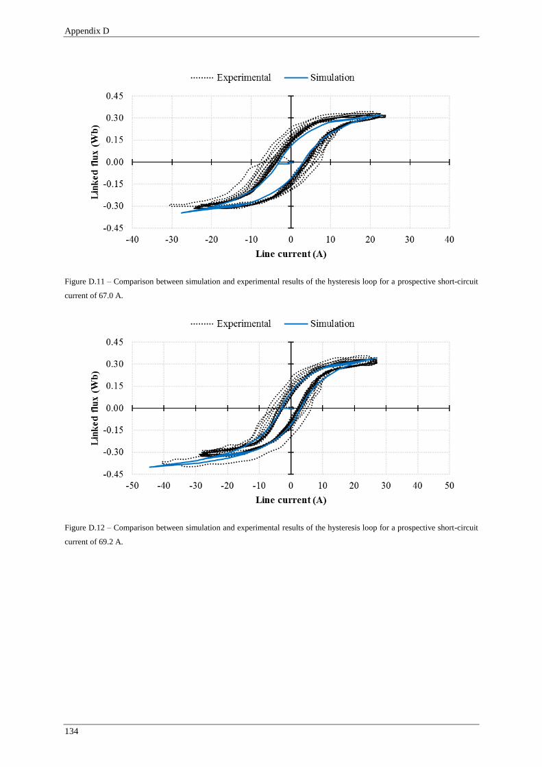
Appendix D
134
Figure D.11 – Comparison between simulation and experimental results of the hysteresis loop for a prospective short-circuit
current of 67.0 A.
Figure D.12 – Comparison between simulation and experimental results of the hysteresis loop for a prospective short-circuit
current of 69.2 A.

Appendix D
135
Simulated and Experimental Superconducting Current
Figure D.13 – Comparison between simulation and experimental results of the superconducting current for a prospective
short-circuit current of 40.2 A.
Figure D.14 – Comparison between simulation and experimental results of the superconducting current for a prospective
short-circuit current of 60.5 A.

Appendix D
136
Figure D.15 – Comparison between simulation and experimental results of the superconducting current for a prospective
short-circuit current of 67.0 A.
Figure D.16 – Comparison between simulation and experimental results of the superconducting current for a prospective
short-circuit current of 69.2 A.

Appendix D
137
Simulated and Experimental Temperature in Superconductor
Figure D.17 – Comparison between simulation and experimental results of the temperature in superconductor for a prospective
short-circuit current of 40.2 A.
Figure D.18 – Comparison between simulation and experimental results of the temperature in superconductor for a prospective
short-circuit current of 60.5 A.

Appendix D
138
Figure D.19 – Comparison between simulation and experimental results of the temperature in superconductor for a prospective
short-circuit current of 67.0 A.
Figure D.20 – Comparison between simulation and experimental results of the temperature in superconductor for a prospective
short-circuit current of 69.2 A.