CONTRADICTORY TRENDS IN GLOBAL INCOME INEQUALITY:

A TALE OF TWO BIASES

by Steve Dowrick*School of Economics, Australian National University

and

Muhammad Akmal

Australian Bureau of Agriculture and Resource Economics

Did global income inequality rise or fall over the last decades of the twentieth century? The answerdepends on how cross-country income comparisons are made. Exchange rate comparisons suggest thatinequality rose whilst the purchasing power comparisons of the Penn World Table suggest it fell. We showthat both measures of real incomes lead to biased international income comparisons. Exchange rate com-parisons ignore the relative price of non-tradables, whilst the fixed price method underlying the PennWorld Table is subject to substitution bias. The contradictory trends are due to growing dissimilaritybetween national price structures increasing the degree of bias in each method. When we correct theincome data to eliminate bias we find no compelling evidence of a significant change in world inequality.

1. Introduction

An apparent increase in inequality in international income distribution overthe 1980s was highlighted by Korzeniewicz and Moran (1997) and by the UnitedNations Development Program in the Human Development Report (UNDP,1999). Whilst the former is reluctant to draw strong conclusions about underlyingcauses, the UNDP report argues for international policies to mitigate risinginequality caused by economic globalization. Both studies rely on foreign exchangerates (FX) to convert incomes to a common currency.

For some purposes, such as assessing a nation’s capacity to repay foreign debt orits bargaining power in international trade negotiations, the FX income comparisonmay well be appropriate. For the purpose of measuring inequality in living standards,however, we need to take account of the real purchasing power of national curren-cies which typically differs from the purchasing power implied by the exchange rate.

A number of studies1 have shown world inequality to be falling when incomecomparisons are made using the purchasing power parities of the Penn World

201

Review of Income and WealthSeries 51, Number 2, June 2005

Note: The authors thank the editor, Stephan Klasen, and two anonymous referees for their commentsand suggestions. We are grateful for additional comments from participants at the WIDER 2003 Confer-ence and from participants in seminars at Griffith University and the Australian National University.

*Correspondence to: Steve Dowrick, School of Economics, Copland Building (26), AustralianNational University, ACT 0200, Australia (Steve.Dowrick@anu.edu.au).

1An exception is Milanovic (2002) who reports rising inequality between 1988 and 1993. AlthoughMilanovic adjusts for purchasing power parities, his income definition is different from all the otherstudies, which are based on concepts of national or domestic income. He uses household incomederived from survey data. Bourguignon and Morrisson (2002) find that the direction of change in inter-country inequality between 1980 and 1992 depends in part on the choice of inequality measure. TheirTable 2 shows a small rise in the Theil index whilst both the mean logarithmic deviation and the stan-dard deviation of log income decline. They use a different measure of purchasing power parity, relyingon the estimates of Maddison (1995).

Table (PWT5.6)2: Firebaugh (1999) reports that both the Theil and Gini indexesof inter-country inequality decline between 1965 and 1989, confirming the find-ings of Schulz (1998) who also reports a decrease in the variance of log income.These results are confirmed by Melchior et al. (2000), by Sala-i-Martin (2002b),and by our own calculations using PWT data, which are illustrated in Figure 1.We follow previous studies in using population-weighted measures of inequality,conceiving inequality as a function of income gaps between people or households.(If we focus on the national economy as the unit of observation, we find that PWTincomes have been diverging.)

It is well established that international currency markets tend to undervaluethe domestic purchasing power of currencies of low productivity/low incomecountries. This is the common experience of international travelers who find thattheir money will go much further in India or Indonesia than it will in WesternEurope. The phenomenon has been analyzed by Balassa (1964), Samuelson (1964)and Bhagwati (1984). Real wages are low in countries with low labor productiv-ity, so non-traded labor-intensive services are cheap relative to capital-intensivetraded goods. Market exchange rates are more likely to equate prices across coun-tries in the traded sector than in the non-traded sector of the economy. Conse-quently, markets tend to undervalue the domestic purchasing power of thecurrencies of poor countries. An important implication of this “traded sector bias”

202

0.50

0.55

0.60

0.65

0.70

0.75

1980

1982

1984

1986

1988

1990

1992

1994

1996

Gin

i Co

effi

cien

tFore ign Exchangeincom e com parisons

Penn World Table income comparisons

Figure 1. Inter-country Income Inequality 1980 to 1987

Source: World Bank (2001), Global Development Network database: Macro Time Series.Notes:1. “Foreign Exchange Income” is GDP at market prices (current US$) divided by population.

Dollar figures for GDP are converted from domestic currencies using single year officialexchange rates.

2. “Penn World Table Income” is Real GDP Per Capita in constant dollars (international prices,base year 1985) derived from Penn World Table 5.6. Missing data are calculated by GDN from1985 GDP per capita and GDP per capita growth rates using Global Development Financeand World Development Indicators.

3. Gini coefficients are calculated on per capita GDP for 115 countries using population weights.

2See Summers and Heston (1991).

is that foreign exchange (FX) income comparisons, because they understate thereal incomes of poorer economies, will overstate the degree of internationalinequality.

Alternatives to FX income comparisons rely on the estimation of purchasingpower parities. A massive research effort, based on detailed price surveys in manycountries under the auspices of the International Comparison Program (ICP), hasresulted in the publication of the Penn World Table (PWT) which provides readyaccess to measures of real GDP per capita at constant international prices for overone hundred countries. These data are commonly referred to as PPP (purchasingpower parity) measures of real income.

Many users of the PWT data are unaware, however, that attempts to measure purchasing power are problematic. The PWT are based on the Geary-Khamis (GK) method of construction of “average international prices” for abenchmark year. The GDP of each country in each year is valued at these fixedprices. However, constant price valuations introduce systematic bias by ignoringconsumers’ ability to substitute towards goods and services that are locally cheap.The progenitors of the Penn World Table describe the problem of substitution biasthus:

The issue arises out of a familiar problem in price and quantity index numberconstruction. . . . Valuation at other than own prices tends to inflate the aggre-gate value of the bundle of goods because no allowance is made for the sub-stitutions in quantities toward the goods that are relatively cheap. . . . Thepractical importance of this issue . . . may loom large in comparisons betweencountries that have widely divergent price and quantity structures. (Kravis et al., 1982, p. 7)

Use of the PWT estimates of international incomes, whilst avoiding thetraded sector bias in the FX income data, introduces substitution bias in its place.We suspect that this issue may be very significant when it comes to assessing thelevel of and trends in world inequality, because we know that the price and quan-tity structures in the world’s poorest economies are very different from those typical of the richer industrialized economies, and we expect that price differen-tials vary over time.

Take, for example, the local currency prices for domestic services and for pas-senger cars, comparing an archetypal labor-intensive service with an archetypaltraded good, in a sample of countries from the 1980 ICP survey. These prices arelisted in the first two rows of Table 1. Local prices are for the real quantity thatcould be purchased for one Geary-Khamis international dollar.

The last row of Table 1 shows the price of domestic services as a ratio of theprice of cars. We find that this price ratio varies by a factor of fifty betweenGermany and India. In Figure 2 we show a plot of this price ratio against per

capita GDP for all of the 60 countries in the 1980 ICP survey, confirming thatthere is a very strong tendency for non-traded services to be much cheaper in lowincome countries than in rich countries.

Given this massive variation in relative prices, the problem of substitutionbias is likely to be substantial. In Section 2 we develop a simple model that cap-tures the biases in both the FX and GK measures of inequality. We find that whilst

203

the Balassa–Samuelson effect causes FX comparisons to exaggerate inequality, theopposite bias is engendered by the GK method of measuring purchasing powerparities. This suggests an explanation for the contradictory observations of trendsin income inequality. If true inequality stays approximately constant, but mea-surement bias increases due to prices becoming less similar over time, then the FXmethod will show rising inequality whilst the GK method will indicate fallinginequality.

204

TABLE 1

Relative Prices of Traded Goods and Non-Traded Services for Five Countries, 1980

Canada Germany Brazil Korea Indonesia India

Per capita GDP at $11,573 $10,390 $3,758 $2,393 $1,101 $605Geary–Khamisinternational prices

Local currency pricesDomestic services 1.44 3.23 7.68 116.2 70.4 0.45Passenger cars 1.00 1.97 22.13 612.3 669.4 14.56

Price ratioServices/cars 1.44 1.63 0.35 0.19 0.11 0.03

Source: World Bank (1993), Tables 4 and 5.Note: Local currency prices are defined as the number of units of a country’s currency required

to purchase the same amounts of goods and services as one U.S. dollar would purchase in the U.S.

0.0

0.2

0.4

0.6

0.8

1.0

1.2

1.4

1.6

1.8

$0 $2,000 $4,000 $6,000 $8,000 $10,000 $12,000

Real GDP per capita

Pri

ce o

f ser

vice

s / c

ars

Figure 2. Price of Domestic Services Relative to Cars, 1980

Source: World Bank (1993).Notes:1. Real GDP per capita is measured in Geary–Khamis international dollars.2. The price ratio is between the categories Domestic Services and Passenger Cars.

We test this hypothesis in Sections 3 and 4. First, we investigate whether ornot national price structures have diverged over the past few decades—a necessarycondition for our hypothesis to hold. Second, we use the multilateral true indexmethodology of Dowrick and Quiggin (1997) to yield true PPP income compar-isons that are free of both substitution bias and traded sector bias to test the conjecture that true inequality has been approximately constant.

2. A Model of Sectoral and Substitution Bias in InternationalIncome Comparisons

In order to better understand the sources of both FX and substitution bias,we construct a simple model of two trading economies. Each produces a non-traded labor-intensive service, S. Country 1 has comparative advantage in pro-ducing an intermediate good, A, which we might think of as an unprocessedagricultural or mineral product. Both countries manufacture a final tradable good,M, using labor and the intermediate good. The production technologies exhibitconstant returns to scale and are identical across countries, except that country-specific private knowledge determines labor productivity in manufacturing. Wedefine country 2 as the high-productivity country.

To keep the model simple we assume Cobb–Douglas production functions inmanufacturing, we treat labor as the only factor of production, we disregard trans-port costs for trading the intermediate and manufactured goods and we assumecompetitive pricing behavior in product and labor markets, including free trade.We assume that all goods and services must be produced, traded and consumedwithin the one time period. The production side of the economy in country i canbe summarized as follows:

(1)

where Zi = (Si, Ai, Mi) represent the domestic output of non-traded services, thetraded intermediate product and the traded manufactured product respectively incountry i; Li

z represents the amount of labor employed in each sector; Aim is the

amount of intermediate input used in manufacturing; and li is the productivity oflabor in country i’s manufacturing sector.

Comparative advantage dictates that country 1 will export the intermediategood and import manufactures. We assume that the productivity differential andrelative population size are such that it is feasible for country 1 to produce all ofthe intermediate good demanded in both countries.

Given constant returns to scale and competitive pricing, we can solve for the domestic price of the manufactured good in country i, Pi

m, in terms of the input prices for labor and the intermediate good, wi and Pi

a (see Appendix fordetails):

(2)

We normalize prices and productivity by setting the wage and productivitylevel in country 1 to unity. We can then use l (>1) without a superscript to repre-

P w P wheremi i i

ai= ( ) ( ) = -( ) ≥- - -m l m a aa a a a1 11 1;

S L A L M L Aisi

ai i

mi

mi= = = ( ) ◊ ( ) < <-

; ;1 1 10 1l aa a

205

sent manufacturing labor productivity in country 2. This allows us to derive theprice vector for country 1 as:

(3)

The exchange rate is E units of currency 2 per unit of currency 1. The priceof the imported intermediate good in country 2 is E. This determines the price ofthe manufactured good, using (2) as:

(4)

Free trade in the manufactured good equalizes prices across countries, requir-ing P2

m = E.P1m = mE. These conditions fully determine the wage in country 2. Setting

the right hand side of (4) equal to mE yields:

(5)

That is to say, productivity-adjusted factor-prices are equalized across thetraded sectors.

By assumption, there are no differences across countries in the productivityof labor in the production of non-traded services. The price of services is simplythe wage. It follows that services are relatively expensive in the high-productivity,high-wage country where the price vector, in units of country 1’s currency, is:

(6)

We analyze demand and welfare by assuming common Cobb–Douglas preferences for the representative consumer-producer who is supplying a unit oflabor inelastically:

(7)

where s and m refer to per capita consumption of services and manufacturedgoods.

The budget share of services is b in each country. Given that per capita incomein each country equals the wage, the per capita consumption bundles are:

(8)

Per capita consumption of services is identical in the two countries, despitethe fact that services are more expensive in country 2, because the income effectof higher manufacturing productivity offsets the price effect. This exact offsettingis an artifact of the Cobb–Douglas production and utility functions, but it is notcrucial to our results. There is higher per capita consumption of manufactures inthe higher productivity country. Thus we can refer to the higher productivitycountry as the high income or richer country.

Evaluating the common utility function (7) at q1 and q2 gives the welfareranking U 2 > U 1. In general the utility ratio, U 2/U 1, is greater than unity but otherwise indeterminate because the utility function is ordinal rather than cardinal. Cardinality is achieved by the money-metric Allen welfare index:

q q1 1 1 2 2 21 1∫ [ ] =

-ÈÎÍ

˘˚̇

∫ [ ] =-( )È

Î͢˚̇

s m s m, , ; , ,bb

mb

l bm

U s m s mi i i i i,( ) = ( ) ( ) < <-b b b10 1

P2 1∫ ( )E l m, ,

w E2 = l

Pw

Em2

21= Ê

ˈ¯

-ml

aa

P1 1 1 1 1 1∫ ( ) = ( )P P Ps a m, , , , m

206

(9)

which compares the minimum expenditures required to achieve utilities U 2 and U 1

at some reference price vector, pr. In our case, where the assumed preference func-tion is homothetic, the Allen index is independent of the reference price vector.The true per capita income ratio between country 2 and country 1 is the uniquevalue:

(10)

These findings are summarized in the following proposition which is a restate-ment of the Balassa–Samuelson results:

Proposition 1: With free trade in intermediate and manufactured goods andcompetitive pricing, the country with higher productivity in manufacturingwill exhibit the following features:

(i) per capita utility is higher;(ii) non-traded labor-intensive services are more expensive relative to traded

goods.

Foreign Exchange Rate Comparisons of Incomes

In this model, per capita National Income and Gross Domestic Product areidentical and, measured in local currencies, are simply equal to the wage. So theGDP or income ratio that is obtained from exchange rate comparison is simplythe ratio of the wage levels expressed in a common currency. Noting that the wagein country 1 is normalized to unity and substituting in equation (5) for wages incountry 2, we derive the FX income ratio:

(11)

Proposition 2: Non-traded sector bias in FX comparisons

(i) Market exchange rates overstate true international income differentials.(ii) The magnitude of the bias is an increasing function of: (a) the underly-

ing productivity differential between the countries; and (b) the domesticexpenditure share of the non-traded sector.

Proof: From (10) and (11), given 0 < b < 1 and l > 1,

(12)

The first part of this proposition simply restates the more general result foundin Samuelson (1974). The overstatement of true income differentials is due to“traded sector bias.” The market exchange rate equates purchasing power of cur-rencies over the traded good but overstates the purchasing power of the currencyover non-traded services in the rich country where non-traded labor-intensive ser-

FX2 1

2 1 1:

:A= >lb

FX2 12

1: = =

w

Ewl

AU

U2 1

2

11 1: ∫

( )( ) = >-qq

l b

Ae U

e Ur

r

r

2 12

1: ,

,∫

( )[ ]( )[ ]q pq p

207

vices are relatively expensive. It follows that the use of market exchange rates tocompare incomes exaggerates the degree of international inequality. Our parame-terization of the model leads to the unsurprising conclusion that the extent of thisbias is increasing in both the productivity differential, l (which causes the realwage differential) and the size of the non-traded sector, b (where the real wage differential affects the relative price).

Geary–Khamis Comparisons of Incomes

We turn now to the measurement of the international income ratio by theGeary–Khamis (GK) method which is used to construct the Penn World Table.This method values each country’s GDP bundle at “international prices.” Theinternational price of manufactures, relative to services, is constructed as a quan-tity-weighted average of the relative prices of all the countries in the GK system.For the purposes of our model we have considered only two countries, but we canallow for other countries with a range of productivity levels in the GK system.

We represent the GK final consumption price vector as:

(13)

Referring back to equation (6), we see that the relative price of manufactures,m/g, corresponds to the relative price that would be found in a country where themanufacturing productivity parameter is g. If the GK system is dominated bycountries more productive than country 2, g will be greater than l. If the rest ofthe world is less productive than country 1, g will be less than unity.

The Geary–Khamis measure of real GDP per capita for country i is the per

capita consumption bundle evaluated at international prices: (qi)¢PGK. Evaluatingthe consumption bundles given in (8) at prices [g, m], the GK income ratio betweencountries 1 and 2 is:

(14)

Whether this under- or over-states the true income ratio depends on the valueof g. We summarize the relationship in our third proposition.

Proposition 3: Substitution bias in Geary–Khamis comparisons

(i) A bilateral international comparison of per capita income which valuesexpenditure at constant prices will understate the true income differen-tial if the constant price vector corresponds to that of the high produc-tivity country, or the prices of an even richer country.

(ii) A constant price comparison will overstate the true income differentialif the constant price vector corresponds to that of the low productivitycountry, or the prices of an even poorer country.

(iii) The bias is greater, the less similar is the reference price vector withrespect to the comparison country prices.

(iv) Where (i) or (ii) holds, the magnitude of the bias is an increasing function of the underlying productivity differential between the two comparison countries.

GKGKGK

2 12

1

11

: gg

g

g

g( ) ∫

( )( )

=+ -( )+ -( )

b b lb b

P GK GK GKg P P gS M( ) ∫ [ ] = [ ], , m

208

Proof : See Appendix for details. The ratio of the constant price (GK) income ratioto the true income ratio is R(g):

(15)

R(g) measures the proportional bias in the GK index, with R = 1 represent-ing no bias. Evaluating (15) gives R(1) > 1 and R(l) < 1 (for l > 1 and 0 < b < 1,as assumed). Differentiating (15), Rg < 0. Hence (i) and (ii).

R is less than 1 for all g > l. As g rises above l (i.e. as the reference pricevector becomes less similar to prices in countries 1 and 2) R falls. R is greater than1 for all g < 1. As g falls below unity (i.e. as the reference price vector becomes lesssimilar to prices in countries 1 and 2), R rises. Hence (iii).

R is decreasing/increasing in the productivity differential, l, as l < g or l > g. Hence (iv).

Proposition 3 clarifies the nature of substitution bias in fixed price compar-isons. It is well known that the use of country 1’s prices is likely to exaggeratecountry 2’s welfare—since goods that are in high demand in 2, because of theirrelative cheapness, will be overvalued at 1’s prices. In other words, the Laspeyresquantity index is usually larger then the Paasche index—and must be so if theunderlying preferences are common and homothetic. It follows that valuingdemand at country 1’s prices will tend to overstate true inequality, if 1 is poorerthan 2, and vice versa. This implication of substitution bias in the measure-ment of inequality is sometimes referred to as the Gerschenkron Effect, after Gerschenkron (1951).

Nuxoll (1994) has shown that the Gerschenkron effect will apply when theincome ratio between country 1 and country 2 is measured at the prices of somethird country, if relative prices and quantities are inversely correlated across allthree countries. Proposition 3 formalizes Nuxoll’s result in the context of anexplicit model where prices, quantities and the true income ratio are endogenouslydetermined by tastes and technology.

It follows from Proposition 3 that the direction and magnitude of bias in GKbilateral income ratios depends on whether the GK price vector corresponds mostclosely to the relative price structures of high income (high productivity) coun-tries—in which case most bilateral ratios will be underestimated—or whether theGK price vector corresponds most closely to the relative price structures of lowincome (low productivity) countries—in which case most bilateral ratios will beoverestimated. The former situation is most likely to apply given that the GKmethod weights each country’s price vector by its share in total GDP, implying thatmore weight is given, ceteris paribus, to the price vectors of the richer countries.

The predicted magnitude of both fixed-price substitution bias and FX bias isillustrated in Figure 3 for the case where non-traded services comprise half of totalexpenditure, i.e. b = 0.5. The horizontal axis measures l, the productivity differ-ential between the manufacturing sectors of the two countries, which is illustratedfor values between one and ten. The uppermost line shows the extent of positivebias in the foreign exchange comparison: FX2:1/A2:1. If the productivity differen-tial is large, for example if l = 10, FX comparisons overstates the true income ratio

R gg

A

g

g( ) ∫

( )=

+ -( )+ -( )[ ] -

GK 2 1

2 1 1

11

:

:

b b lb b l b

209

more than threefold. The lower line shows bias in GK income comparisons,GK2:1/A2:1, using constant prices that correspond to those of a high productivitycountry with a productivity parameter, g, of 30. In this case the GK method under-states the true income ratio. This bias can be substantial; for example, it reachesa ratio of 0.4 when l = 10.

The biases illustrated here refer to the measurement of the income ratiobetween a pair of countries. We expect to find similar bias in measures of multi-lateral inequality because most measures are constructed from bilateral ratios.

3. Can We Explain Increasing FX Inequality andDecreasing PWT Inequality?

We have demonstrated that there are potentially serious biases in the two mostcommonly used methods of comparing international incomes. Moreover, it islikely that the biases may work in opposite directions, with the Foreign Exchange(FX) income measure overstating the true level of inequality whilst theGeary–Khamis (GK) measure understates inequality. This occurs when the GKmethod is evaluating GDP at a set of “international” prices that correspond to theprice structure of a high productivity economy.

Nuxoll (1994) analyzes bilateral income ratios and reports on page 1431 that the international prices underlying the 1980 ICP measures of real GDP corre-spond to those of “some moderately prosperous” country such as Hungary or

210

0.0

0.5

1.0

1.5

2.0

2.5

3.0

3.5

1 2 3 4 5 6 7 8 9 10

Productivity Differential in Manufacturing (l)

FX Income Ratio / True Ratio

GK(30) Income Ratio / True Ratio

Figure 3. Predicted Exchange Rate Bias and Substitution Bias

Note: Predicted biases are calculated according to equations (12) and (15) with the parametersset as b = 0.5 and g = 30.

Yugoslavia, with per capita GDP of around $5,000. We apply a similar analysis toa multilateral measure, the variance of log income. We use the 1980 ICP data toconstruct measures of the variance of constant price log GDP per capita acrossthe 60 countries, using first the prices of the U.S. and then the prices of each ofthe other 59 countries. The results are shown in Figure 4, with the variance on thevertical axis and the log of GK GDP per capita for the reference country on the horizontal axis. As predicted by our Proposition 3, the higher is the income ofthe reference country, the lower is the measured variance of log income acrosscountries. The measured variances range from 0.85 to nearly 1.6. The empiricalrelationship is very strong with the linear regression line explaining more than 80percent of the variation in measured inequality.

In Figure 4 we have also illustrated the variance of 1980 log incomes fromPWT5.6 for the same countries, represented by the solid horizontal line at 1.02.This coincides with the regression line at a log income of 9.1, corresponding toincome of exp(9.1) ª $9,000. It appears that the GK constant international pricevector underlying this version of the Penn World Table is most closely representedby the price structure of a relatively rich country such as Hong Kong, Japan orthe U.K. with 1980 per capita income around $9,000. This is not surprising, sincethe rich OECD economies, with average income levels above $13,000, accountedfor more than half of world GDP, exerting a dominant influence on the con-struction of the GK international price vector. More than two thirds of the coun-tries have income levels lower than $9,000, suggesting that most of the GK incomeratios are likely to be biased downwards, understating the true level of inequal-ity—as demonstrated by Dowrick and Quiggin (1997) and by Hill (2000).

We have shown that the degrees of bias in both FX and GK income measuresare likely to increase as the true level of inequality increases. This suggests one

211

y = 2.53 - 0.17x R2 = 0.81

0.8

0.9

1.0

1.1

1.2

1.3

1.4

1.5

1.6

1.7

5.0 6.0 7.0 8.0 9.0 10.0

Log income of reference country

vari

ance

at

refe

ren

ce c

ou

ntr

y p

rice

s

Variance ofPWT Incomes

Figure 4. Variance of 1980 Log Real GDP Per Capita At Reference Country Prices

Source: World Bank (1993) Tables 4 and 5 for 1980 ICP data.Notes:1. “Income” is real GDP at Geary-Khamis international prices.2. The “variance at reference country prices” is the variance of log GDP per capita measured

for each country at the prices of the reference country.

possible explanation for the conflicting messages coming from the analysis of FXand GK income inequality. If true inequality is rising over time, both the upwardFX bias and the downward GK bias will increase. It follows that the rate ofincrease in inequality will be exaggerated by FX measures and understated by theGK measure.

On its own, this hypothesis is not enough to explain why FX inequality hasbeen trending up and GK inequality trending down. In the simple model ofSection 2, where there are only two consumption goods, both the FX and GKmeasures move in the same direction when true inequality changes. In reality,however, there is a multiplicity of goods and relative prices which are influencedto varying degrees by trade restrictions, by international differences in productiv-ity and factor endowments, by monopoly pricing, by government regulation, etc.For instance, Falvey and Gemmell (1996) report that international differences inthe price of services are explained by differences in factor endowments as well asdifferences in total factor productivity and Dowrick and Quiggin (1997) find thatthe degree of substitution bias in fixed-price income comparisons is increasing inthe dissimilarity between countries’ price vectors. It follows that the degree of biasin both FX and GK measures is likely to increase not only when underlying pro-ductivity differentials increase but also when national price structures diverge forother reasons. Thus we propose an explanation for the riddle of GK inequalityfalling whilst FX inequality rises:

Conjecture:

(i) True inequality changed little between 1980 and 1993; but(ii) national price structures became less similar;

causing the FX measure of world inequality to rise and the GK measure ofinequality to fall.

Firebaugh (1999) discounts this possibility, citing the finding of Dowrick andQuiggin (1997) that price structures had become more similar over the 1980s.Those findings were, however, only for the OECD countries where price conver-gence had been promoted by European economic integration. There is no pre-sumption of price convergence across the rest of the world or between OECDcountries and the rest.

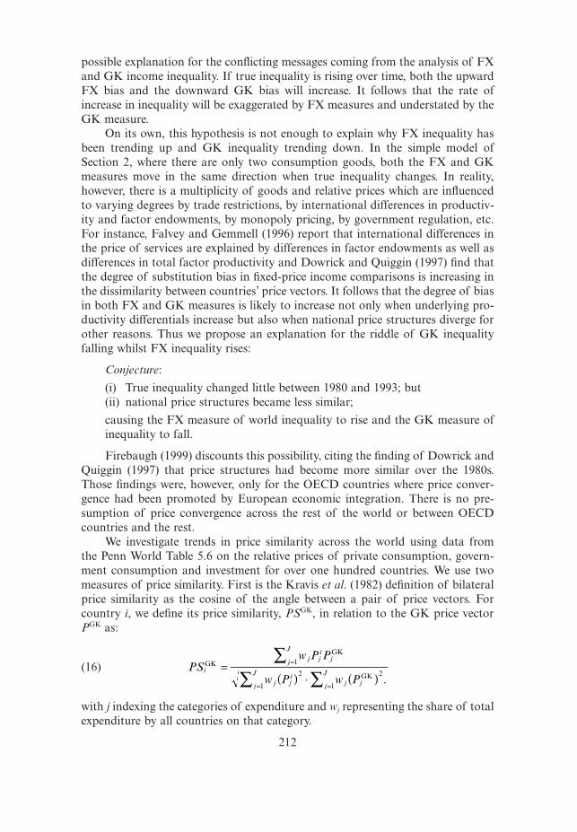
We investigate trends in price similarity across the world using data from the Penn World Table 5.6 on the relative prices of private consumption, govern-ment consumption and investment for over one hundred countries. We use twomeasures of price similarity. First is the Kravis et al. (1982) definition of bilateralprice similarity as the cosine of the angle between a pair of price vectors. Forcountry i, we define its price similarity, PSGK, in relation to the GK price vectorPGK as:

(16)

with j indexing the categories of expenditure and wj representing the share of totalexpenditure by all countries on that category.

PSw P P

w P w Pi

j ji

jj

J

j ji

j

J

j jj

J

GK

GK

GK=

( ) ◊ ( )=

= =

ÂÂ Â

1

2

1

2

1.

212

Second, we use the Diewert (2002) bilateral index of relative price dissimilar-ity (the unweighted asymptotically linear index), D(x, g), which is defined as:

where x represent the price vector of country x and g represents the GK pricevector, and i = 1 . . . n indexes the commodities which make up the GDP bundle.Note that m is defined as the geometric mean of x relative to g, and the dissimi-larity index is the sum of the normalized price ratios and their reciprocals, adjustedto make the index equal zero when the prices in country x are an exact multipleof the GK prices.

Figure 5 displays the time trends between 1980 and 1991 for the cross-countrymeans of the Diewert and KHS indices. The time trends are almost mirror imagesof each other because the former index measures dissimilarity rather than simi-larity. It is evident that between 1980 and 1991 price structures became markedlyless similar/more dissimilar,3 confirming the second part of our conjecture.

Dn

g

x

x

g

x

g

i

i

i

ii

n

i

i

n

i

n

x g,( ) = + -ÊË

ˆ¯

= ÊË

ˆ¯

=

=

Â

’

12

1

1

1

mm

m

213

Price Similarity and Dissimilarity Indices, 1980 to 1991

0.938

0.940

0.942

0.944

0.946

0.948

0.950

0.952

0.954

0.956

1980 1981 1982 1983 1984 1985 1986 1987 1988 1989 1990 1991

0.19

0.20

0.21

0.22

0.23

0.24

0.25

0.26

0.27

0.28

KHS Similarity Index (left scale)

Diewert Relative Dissimilarity (right scale)

Figure 5. Price Similarity and Dissimilarity Indexes Across 131 Countries, 1980 to 1991

Source: Prices of private consumption, government consumption and investment are from PennWorld Table 5.6.

Note: The index number formulae are equations (16) and (17). There are 131 country observa-tions 1980 to 1989, 102 for 1990 and 100 for 1991.

3The sample of countries is held constant at 131 for 1980 to 1989, dropping to 112 and 100 in1990 and 1991 respectively due to missing price data in PWT5.6. The results are very similar if werestrict our sample to the 98 countries for which data are available for all twelve years.

(17)

To investigate the other part of our conjecture we need measures of interna-tional incomes that are free of both substitution bias and traded sector bias.Dowrick and Quiggin (1997) develop a method that achieves this, based on theeconomic index number approach of Afriat (1984). This method involves search-ing for multilateral index numbers satisfying the condition that the bilateral ratioslie within the Paasche and Laspeyres bounds, making use of the algorithmdescribed by Varian (1983). If such an index exists, the underlying price and quan-tity observations are consistent with optimizing choice by a representative con-sumer with homothetic preferences and the index numbers can be interpreted asan Allen welfare index. We apply this method to the 1980 and 1993 ICP bench-mark studies.4

We find that for a majority of countries (52 of the 60 countries in the 1980benchmark study, and 49 of the 53 countries in the 1993 study) the ICP observa-tions on prices and quantities do satisfy the Afriat test for common homotheticpreferences. For this set of observations the Allen money-metric utility compar-isons, E(u(qi), pr) / E(u(qj), pr), are independent of the choice of pr. We then followDowrick and Quiggin (1997) in constructing the Ideal Afriat Index, which givesutility-consistent income ratios5 which are free of substitution bias, reflecting truepurchasing power. We refer to this measure as Afriat income or, following Afriat(1984) and Dowrick and Quiggin (1997), as “true” income.

We note the finding of Ackland et al. (2004) that the EKS index is close tobeing a true Afriat index when applied to the 1993 ICP data. We confirm thisfinding for the 1980 ICP data where the variance of log income measured by theEKS index is 1.18, only slightly higher than the variance of log income measuredby the Ideal Afriat Index. Indeed, a linear regression of the former index on thelatter yields the result: ln EKS = 1.009 ln Afriat, R2 = 0.9989. These results suggestthat the subsequent data analysis would be altered very little if we were to substi-tute the EKS index for the Afriat index. We prefer to use the Afriat index becauseit is consistent with generalized homothetic preferences, as in our theoreticalmodel, and because we are able to test whether the data are consistent with suchpreferences.

Estimating Afriat GDP for Non-Benchmark Countries

We are able to calculate true GDP per capita for all of the countries includedin the 1980 and 1993 International Comparison (ICP) surveys, using the minimumof the Laspeyres valuations for those countries outside the homothetic sets as recommended by Dowrick and Quiggin (1997). However, in order to get genuinelyrepresentative estimates of world inequality, it is necessary to increase populationcoverage, requiring the extension of PPP estimates to non-benchmark countries.

214

4The 1993 ICP data have been made available by the World Bank (2000) on a regional basis. Weunderstand that the Bank has not published the global estimates. We merged the regional data sets,using common countries to scale the price and quantity data, to create our own global estimates.We have also used ICP data published by World Bank (1993) and time-series data published on theInternet (World Bank, 2001).

5The Afriat method yields multiple sets of utility ratios with defined upper and lower bounds. Forthe purposes of this paper, we use the mid-points of the multilateral bounds, yielding the Ideal AfriatIndex.

This is especially important because China is not covered in either of the ICPsurveys and India is only in the 1980 benchmark.

In order to predict true incomes for non-benchmark countries, we use a pro-cedure developed by Kravis et al. (1982)6 who use ICP benchmark data to estimatea regression model with GK income as the dependent variable and FX income asan explanatory variable.

Our model suggests that FX overstates true income for poorer countries. Sub-stituting equation (11) into (10), and normalizing true income in country 1 tounity, implies that true income per capita in country i, Ai, is:

(18)

We use this log-linear relationship as the basis of a regression model, aug-menting it with a variable, OPEN, capturing the exposure of the country to foreigntrade. Deviations between FX and A are driven by price differences between thetraded and non-traded sectors of the economy—so where the traded sector con-stitutes a larger proportion of GDP, we expect the A/FX ratio to be closer to unity.We regress log A on log FX and OPEN for each of the two benchmark years sep-arately, testing for functional form by including the square of log FX and the inter-action of OPEN with log FX. Then, data for the two years is combined to obtainpooled estimates.

The regression results are reported in Table 2. Following tests for het-eroscedasticity, the 1980 equation and the pooled model were estimated usingweighted least squares whereas the 1993 equation was estimated by OLS.

The logarithm of FX income is highly significant in all equations. Asexpected, the coefficient is less than unity—varying between 0.6 and 0.8 accord-ing to the sample—implying that the true income distribution is less dispersed thanthe distribution of FX income.

The square of log FX adds significant explanatory power to the regressiononly in the 1980 sample. The openness variable is statistically significant in the1993 regression, along with the interaction term, implying that there is less of agap between FX income and true income in economies that are more exposed toworld trade. The explanatory power, as defined by 2, is close to 97 percent forthe 1993 sample and the standard error of the regression is around 16 percent,which is very similar to the standard errors for the Kravis et al. (1982) regressionreported in the final column of Table 2 and the regressions underlying the con-struction of PWT version 5.6 as reported in the December 1994 update to Appen-dix B of Summers and Heston (1991). The 1993 data are displayed in Figure 6along with the predicted value of the regression. We see that a linear relationshipbetween log A and log FX, as predicted by equation (18), fits the data reasonablywell, with only minor additional explanatory power coming from the additionalvariables.

R

A A FXi i i i= ( ) fi = -( ) < <-FX

11 0 1

b b bln ln ;

215

6Our approach to estimating real incomes in non-benchmark countries is similar to that reportedin Appendix B for Summers and Heston (1991), except that they use various additional price surveys.An alternative approach used by Bergstrand (1991) uses the relative productivity levels in traded andnon-traded sectors as an additional explanatory variable, but such data are not available for the non-benchmark countries.

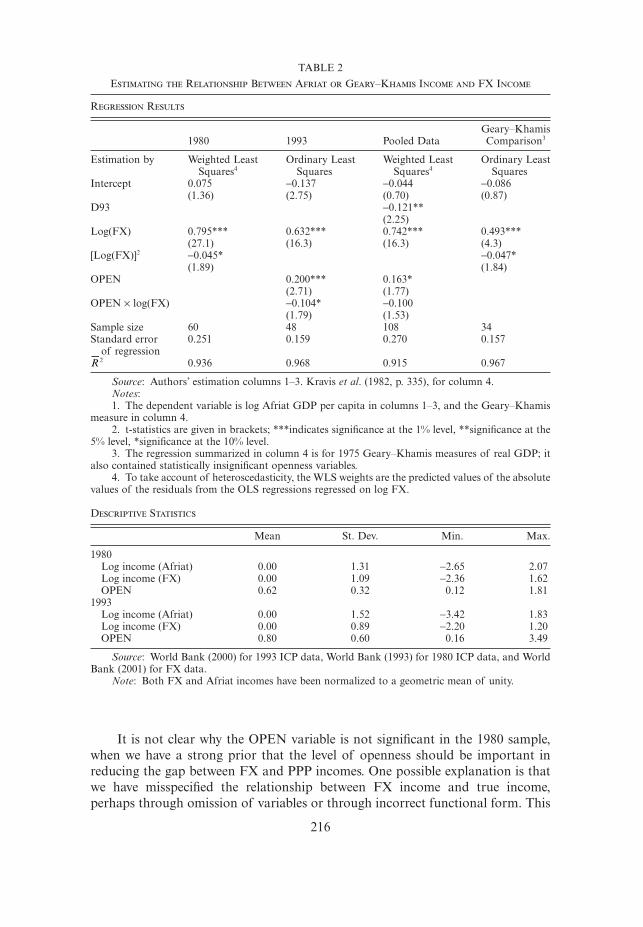
It is not clear why the OPEN variable is not significant in the 1980 sample,when we have a strong prior that the level of openness should be important inreducing the gap between FX and PPP incomes. One possible explanation is thatwe have misspecified the relationship between FX income and true income,perhaps through omission of variables or through incorrect functional form. This

216

TABLE 2

Estimating the Relationship Between Afriat or Geary–Khamis Income and FX Income

Regression Results

Geary–Khamis1980 1993 Pooled Data Comparison3

Estimation by Weighted Least Ordinary Least Weighted Least Ordinary LeastSquares4 Squares Squares4 Squares

Intercept 0.075 -0.137 -0.044 -0.086(1.36) (2.75) (0.70) (0.87)

D93 -0.121**(2.25)

Log(FX) 0.795*** 0.632*** 0.742*** 0.493***(27.1) (16.3) (16.3) (4.3)

[Log(FX)]2 -0.045* -0.047*(1.89) (1.84)

OPEN 0.200*** 0.163*(2.71) (1.77)

OPEN ¥ log(FX) -0.104* -0.100(1.79) (1.53)

Sample size 60 48 108 34Standard error 0.251 0.159 0.270 0.157

of regression2 0.936 0.968 0.915 0.967

Source: Authors’ estimation columns 1–3. Kravis et al. (1982, p. 335), for column 4.Notes:1. The dependent variable is log Afriat GDP per capita in columns 1–3, and the Geary–Khamis

measure in column 4.2. t-statistics are given in brackets; ***indicates significance at the 1% level, **significance at the

5% level, *significance at the 10% level.3. The regression summarized in column 4 is for 1975 Geary–Khamis measures of real GDP; it

also contained statistically insignificant openness variables.4. To take account of heteroscedasticity, the WLS weights are the predicted values of the absolute

values of the residuals from the OLS regressions regressed on log FX.

Descriptive Statistics

Mean St. Dev. Min. Max.

1980Log income (Afriat) 0.00 1.31 -2.65 2.07Log income (FX) 0.00 1.09 -2.36 1.62OPEN 0.62 0.32 0.12 1.81

1993Log income (Afriat) 0.00 1.52 -3.42 1.83Log income (FX) 0.00 0.89 -2.20 1.20OPEN 0.80 0.60 0.16 3.49

Source: World Bank (2000) for 1993 ICP data, World Bank (1993) for 1980 ICP data, and WorldBank (2001) for FX data.

Note: Both FX and Afriat incomes have been normalized to a geometric mean of unity.

R

poses a problem when it comes to predicting true incomes for the non-benchmarkcountries in each year. Should we use the particular coefficients for that year, orshould we use the coefficients from the pooled regression? The former method mayyield more accurate predictions for each particular year, but it creates further prob-lems. The object of the exercise is to compare levels of true income inequalitybetween 1980 and 1993. If we are using two different models to predict trueincomes for non-benchmark countries, we cannot be sure whether any changes inestimated inequality are due to changes in the real income distribution or to thedifferent methods used for predictions. Because we are primarily interested in theintertemporal comparison we focus on the results from the pooled regressions. Werecognize that the possible misspecification of the exact relationship reduces theaccuracy of the incomes predicted for non-benchmark countries, noting thatsimilar problems apply to the PWT estimates of real income.

Different Measures of Inequality

We use four alternative measures of inequality—Gini (G), Theil (T), thesquared coefficient of variation (CV2) and the variance of logarithmic income (L).Firebaugh (1999) shows each measure can be represented by a distance functionof the form:

217

–4

–3

–2

–1

0

1

2

–4 –3 –2 –1 0 1 2

log FX Income

log

Rea

l Inc

ome

real income

predicted real income

45 degree line

Figure 6. Real Afriat Income vs FX Income, 1993, Actual and Predicted Values

Source: World Bank (2001) for FX Income (GDP per capita at current exchange rates); WorldBank (2000) for 1993 ICP data and authors’ calculations of Real Income (Afriat index of true GDPper capita).

Notes:1. “Predicted real income” is the predicted value of Afriat GDP per capita from the second

regression reported in Table 2.2. All of the inequality measures are population weighted as defined in equations (19) and (20).

(19)

where pi is the share of the i-th country’s population in the total population of allN countries and yi is the ratio between the income per capita of the i-th countryand the average income (per capita) across N countries. We use population weightsto reflect our judgment that a proportional change in per capita income in a populous country such as China or India has more significance for global inequalitythan a similar change in a low population country such as Luxembourg or Iceland.

Firebaugh gives the specific functional forms that distinguish the four indexes:

where E is mean value operator, log is the natural logarithm, qi is the proportionof total population in the N countries that is poorer than country i and Qi is theproportion of population richer than country i.

Intra-Country Inequality

Some studies of world income distribution have analyzed income inequalityacross countries while ignoring the intra-country component: Theil (1979, 1996),Theil and Seale (1994), and Firebaugh (1999). In other studies, however, thewithin-country dimension has been taken into consideration, giving a more accu-rate picture of inequality across all households in the world—as in Berry et al.(1983), Grosh and Nafziger (1986), Chotikapanich et al. (1997), Schulz (1998),Milanovic (2002), Sala-i-Martin (2002a, 2002b), and Bourguignon and Morrisson(2002).

Before considering within-country inequality we begin by analyzing thebetween-country component of global inequality for each of the three incomemeasures: FX, Afriat and PWT. The inequality indexes cover 115 countries with86 percent of world population in 1997. The PPP (Afriat) based indexes are cal-culated for 1980 and 1993 only.

Intra-country inequality measures have been taken from Deininger and Squire(1996) who have put together a data set containing quintile income shares and Gini coefficients classified by country, year, income type (gross or net), coverage(national or sub-national), form of recipient unit (person or household) and,importantly, by data quality. The data set includes 682 observations of the highestquality. Relying almost exclusively on the highest quality data, mostly on quintiledistribution and occasionally on Gini, the four inequality indexes are computedfor 1980 and 1993 for 47 countries.

For many countries Deininger and Squire do not report quintile distributiondata of reliable quality for the two years. In order to increase the number of coun-tries, the distribution data for the closest year, while constraining the departure toat most three years from the year of interest—1980 or 1993, are chosen as a proxy.

G T CV

L

= -( ) = = -( )

= - [ ]{ }

= = =

=

  Â

Â

p y q Q p y y p y

p y E y

i i i i

i

N

i i i

i

N

i i

i

N

i i i

i

N

1 1

2 2

1

2

1

1; log ; ;

log log ,

I p f y mm i m i

i

N

= ( ) ==Â

1

; G, T, CV , L2

218

(20)

This increases the country coverage to 67, covering nearly 70 percent of the worldpopulation in both years.

In a few cases, only the Gini coefficient was available. In these cases weapproximate the underlying quintile distribution using the single-parameter func-tional form of the Lorenz curve suggested by Chotikapanich (1993).7 The meanper capita income for different quintiles are obtained by multiplying the relevantquintile income share with the country’s per capita income and then dividing by0.2, the population share per quintile. We treat each country-quintile, with itsaverage income and appropriate population weight, as a single observation in cal-culating global inequality.8

4. Inequality Results

The upper panel in Figure 7 repeats the illustration of FX and PWT Ginicoefficients across 115 countries, but adds in our estimates of inequality of trueAfriat incomes for 1980 and 1993. Our predictions of bias are confirmed. The FXmeasure overstates the true level inequality whilst the PWT measure understatesit.

With respect to changes over time in the inequality of true incomes, there isa very slight rise in the inter-country Gini coefficient, from 0.615 in 1980 to 0.623in 1993. This finding is not, however, robust to the inequality index employed. Theremaining three panels of Figure 7 display the other indexes of inequality—Theil(7B), CV2 (7C) and the variance of log income (7D). We see a slight reduction inthe variance of log true income, from 1.551 to 1.522, between 1980 and 1993, whilstthe other two measures of inequality register a slight increase.

Estimation Error for Countries not Included in the ICP Benchmark Surveys

Because China was not included in either the 1980 or 1993 International Com-parison Project price surveys, both the PWT and our own Afriat measures of realincome rely on out of sample regression forecasts. Given that China accounts forover one-fifth of world population, it is crucial to analyze the robustness of mea-sured inequality with respect to the prediction errors associated with Chinese realincome. The standard errors of the regressions are at least 15 percent within thesample of benchmark countries—and we expect the error to be even greater whenmaking predictions outside the sample. To check robustness, we calculate upperand lower bounds for real GDP per capita in China by adding or subtracting twostandard errors from the baseline predicting regressions. The results are displayed

219

7Chotikapanich (1993) approximates the Lorenz curve by the following single-parameter specifi-cation: LC = (ekp - 1)/(ek - 1). The corresponding Gini coefficient is given by: G = Î(k - 2)ek + (k +2)˚/k(ek - 1), where p is the population share and k is a parameter, which is required to be greater thanzero. In the first step, the Gini equation is solved for k which then is used to obtain the estimates ofquintile income distribution.

8These approximations, combined with our necessarily imperfect estimation of national incomesfor non-benchmark countries and the more general problems of compiling data from secondarysources—see Atkinson and Brandolini (2001)—mean that there must be a substantial degree of impre-cision in our inequality estimates. The principal interest of this paper, however, lies in comparing resultsfrom different methods of calculating purchasing power comparisons using the same secondarysources.

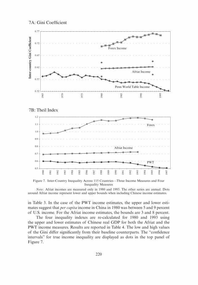
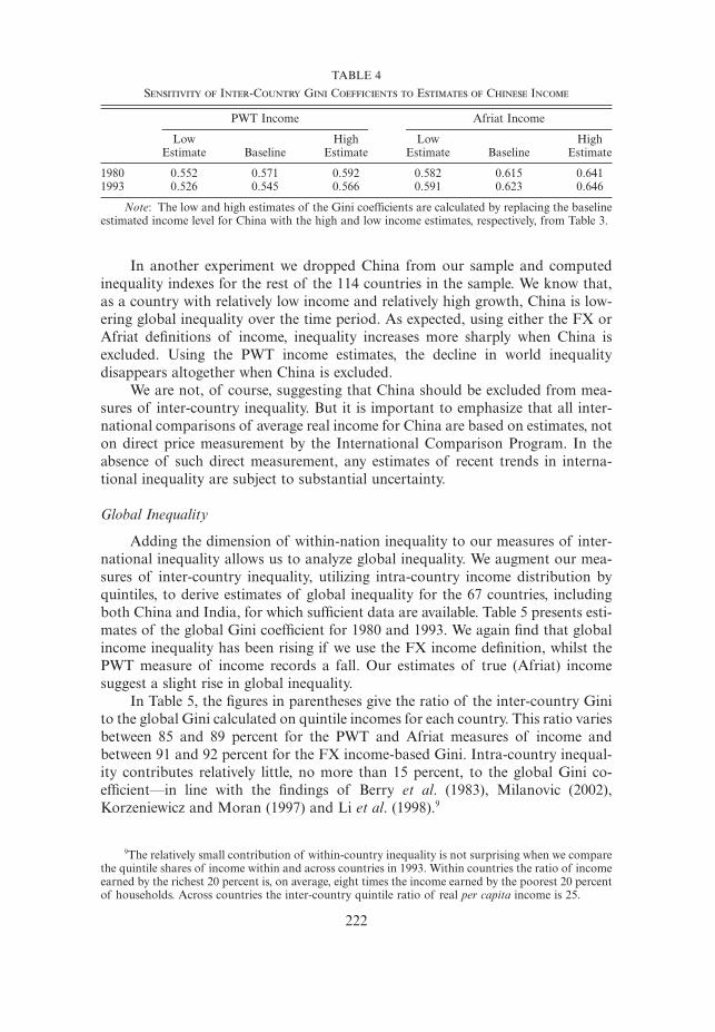
in Table 3. In the case of the PWT income estimates, the upper and lower esti-mates suggest that per capita income in China in 1980 was between 5 and 9 percentof U.S. income. For the Afriat income estimates, the bounds are 3 and 8 percent.

The four inequality indexes are re-calculated for 1980 and 1993 using the upper and lower estimates of Chinese real GDP for both the Afriat and thePWT income measures. Results are reported in Table 4. The low and high valuesof the Gini differ significantly from their baseline counterparts. The “confidenceintervals” for true income inequality are displayed as dots in the top panel ofFigure 7.

220

7A: Gini Coefficient

7B: Theil Index

0.52

0.57

0.62

0.67

0.72

0.77

1965

1970

1975

1980

1985

1990

1995

Inte

r-co

untr

y G

ini C

oeffi

cien

t

Forex Income

Penn World Table Income

Afriat Income

0.5

0.6

0.7

0.8

0.9

1.0

1.1

1.2

1980

1981

1982

1983

1984

1985

1986

1987

1988

1989

1990

1991

1992

1993

1994

1995

1996

1997

Forex

Afriat Income

PWT

Figure 7. Inter-Country Inequality Across 115 Countries—Three Income Measures and FourInequality Measures

Note: Afriat incomes are measured only in 1980 and 1993. The other series are annual. Dotsaround Afriat income represent lower and upper bounds when including Chinese income estimates.

221

7C: Squared Coefficient of Variation

1.3

1.5

1.7

1.9

2.1

2.3

2.5

2.7

2.9

3.1

3.3

3.5

1980

1981

1982

1983

1984

1985

1986

1987

1988

1989

1990

1991

1992

1993

1994

1995

1996

1997

Forex

Afriat Income

PWT

7D: Variance of Log Income

0.6

1.0

1.4

1.8

2.2

2.6

3.0

1980

1981

1982

1983

1984

1985

1986

1987

1988

1989

1990

1991

1992

1993

1994

1995

1996

1997

Forex

Afriat Income

PWT

Figure 7. (continued)

TABLE 3

Estimated GDP PER CAPITA of China (as a percentage of US income)

1980 1993

FX Afriat PWT FX Afriat PWT

Lower prediction 2.6% 4.7% 2.5% 6.7%Baseline 1.7% 4.7% 6.4% 1.5% 4.5% 9.2%Higher prediction 8.5% 8.7% 8.1% 12.6%

Notes:1. The upper and lower predictions for Afriat income are calculated using forecast values from

Regression 3 in Table 2 and adding or subtracting two standard errors of the regression.2. The standard error of regression for the PWT income is taken from Summers and Heston

(1991) who report seven alternative regression equations which are used for prediction depending onthe availability of data on different countries. The median standard error of the regression, 0.15, isused to perform the sensitivity analysis.

In another experiment we dropped China from our sample and computedinequality indexes for the rest of the 114 countries in the sample. We know that,as a country with relatively low income and relatively high growth, China is low-ering global inequality over the time period. As expected, using either the FX orAfriat definitions of income, inequality increases more sharply when China isexcluded. Using the PWT income estimates, the decline in world inequality disappears altogether when China is excluded.

We are not, of course, suggesting that China should be excluded from mea-sures of inter-country inequality. But it is important to emphasize that all inter-national comparisons of average real income for China are based on estimates, noton direct price measurement by the International Comparison Program. In theabsence of such direct measurement, any estimates of recent trends in interna-tional inequality are subject to substantial uncertainty.

Global Inequality

Adding the dimension of within-nation inequality to our measures of inter-national inequality allows us to analyze global inequality. We augment our mea-sures of inter-country inequality, utilizing intra-country income distribution byquintiles, to derive estimates of global inequality for the 67 countries, includingboth China and India, for which sufficient data are available. Table 5 presents esti-mates of the global Gini coefficient for 1980 and 1993. We again find that globalincome inequality has been rising if we use the FX income definition, whilst thePWT measure of income records a fall. Our estimates of true (Afriat) incomesuggest a slight rise in global inequality.

In Table 5, the figures in parentheses give the ratio of the inter-country Ginito the global Gini calculated on quintile incomes for each country. This ratio variesbetween 85 and 89 percent for the PWT and Afriat measures of income andbetween 91 and 92 percent for the FX income-based Gini. Intra-country inequal-ity contributes relatively little, no more than 15 percent, to the global Gini co-efficient—in line with the findings of Berry et al. (1983), Milanovic (2002),Korzeniewicz and Moran (1997) and Li et al. (1998).9

222

TABLE 4

Sensitivity of Inter-Country Gini Coefficients to Estimates of Chinese Income

PWT Income Afriat Income

Low High Low HighEstimate Baseline Estimate Estimate Baseline Estimate

1980 0.552 0.571 0.592 0.582 0.615 0.6411993 0.526 0.545 0.566 0.591 0.623 0.646

Note: The low and high estimates of the Gini coefficients are calculated by replacing the baselineestimated income level for China with the high and low income estimates, respectively, from Table 3.

9The relatively small contribution of within-country inequality is not surprising when we comparethe quintile shares of income within and across countries in 1993. Within countries the ratio of incomeearned by the richest 20 percent is, on average, eight times the income earned by the poorest 20 percentof households. Across countries the inter-country quintile ratio of real per capita income is 25.

Given that intra-country inequality is only a minor component of worldinequality, it is not surprising to find that the global Gini coefficient displays asimilar time trend to the inter-country Gini. The inclusion of within-countryinequality tends to rescale the indexes upwards, without greatly altering rates ofchange over recent years.

The corresponding results for the other three inequality indexes—Theil (T),coefficient of variation squared (V2) and variance of log income (L)—are presentedin Table 6. We find that for each of these indexes the contribution of within-country inequality is proportionally greater than was the case with the Gini index.Nevertheless, the trends identified for the global Gini index, are essentially robustto the choice of inequality index. Global inequality falls between 1980 and 1993for PWT incomes, but it increases for true Afriat income and FX income, accord-ing to all four indexes.

We are concerned, however, that the use of grouped income data may sub-stantially understate the contribution of intra-country inequality to globalinequality. As an experiment, we generated ten thousand log-normally distributedincomes and computed the variance of log income when the income is grouped

223

TABLE 5

Global Income Inequality: Gini Coefficients by CountryQuintiles Across 67 Countries

PWT Income Afriat Income FX Income

1980 0.659 0.698 0.779(86.7%) (88.0%) (90.9%)

1993 0.636 0.711 0.824(85.6%) (87.7%) (92.4%)

Change 1980–93 -3.4% 1.7% 5.8%

Notes:1. The average income of each country quintile is treated as a

single observation. The Gini coefficient is calculated using countryquintile population weights.

2. The numbers in parentheses are the inter-country Gini co-efficients expressed as a percentage of the global coefficient.

TABLE 6

Alternative Measures of Global Income Inequality by Country Quintiles Across 67Countries

PWT Afriat FX

Theil Index1980 0.84 (70.9%) 0.96 (71.5%) 1.25 (77.3%)1993 0.79 (70.4%) 1.01 (71.4%) 1.50 (79.0%)Percent change 1980-93 -6.7% +5.0% +19.5%

Squared CV1980 2.86 (55.0%) 3.34 (54.5%) 4.33 (60.7%)1993 2.73 (55.4%) 3.63 (54.5%) 5.73 (61.9%)Percent change 1980-93 -4.4% +8.7% +32.1%

Variance of log1980 1.74 (65.3%) 2.21 (70.1%) 3.67 (74.7%)1993 1.51 (62.8%) 2.40 (63.4%) 4.23 (72.2%)Percent change 1980-93 -13.3% +8.5% +15.4%

Note: Values in brackets are the between-country index as a percentage of the global index.

into various fractiles—as shown in Figure 8. We find that the variance of logincome grouped into quintiles is 90 percent of the variance of the full sample. Weconclude, therefore, that the quintile income shares that we and other researchershave used are likely to come close to capturing the full contribution of intra-country inequality to world inequality. This conclusion is reinforced by the findingof Sala-i-Martin (2002a) that estimating a Gaussian kernel density function hasminimal impact on measures of global inequality.

Sala-i-Martin (2002b) criticizes our sample selection, based on an earlierversion of this paper,10 on the grounds that “. . . the selection of countries that donot have Gini data is not random. In particular, these are countries that are poorand that have diverged. Excluding these countries from the analysis tends to biasthe results towards finding reductions in world income inequality” (p. 9). Thispoint simply reinforces our conclusion that, once we correct for the bias in thePWT measures of purchasing power parity, there is no convincing evidence of afall in world income inequality over the period in question. Moreover, there is nosuch selection bias in our measures of the inter-country component which domi-nates quintile-based measures of global inequality.

5. Concluding Comments

A preliminary point that emerges from our theoretical and empirical analy-sis is that researchers who want to compare real income levels across countriesneed to be wary of the label “purchasing power parity.” There is no unique conceptof purchasing power, and there are substantial differences in the methods under-

224

0.60

0.65

0.70

0.75

0.80

0.85

0.90

0.95

1.00

0 5 10 15 20 25 30

number of fractiles

Figure 8. Variance of Fractile Income/Variance of Population

Note: Variances are calculated on 10,000 randomly generated log normal incomes which havebeen ordered and averaged over fractiles.

10Whilst criticizing our sample selection procedures, Sala-i-Martin ignores the principal point ofour paper which is that the Penn World Table data, on which he is relying, bias the measurement ofinequality.

lying the construction of widely used data sets which attach this label to theirincome measures. Our preference is to define purchasing power in terms of thecapacity of a representative consumer to attain the same levels of utility when con-fronted with the particular price structure of each country. Using Afriat’s non-parametric tests we are able to construct true income comparisons and todemonstrate that the frequently used Penn World Table data substantially under-state the true level of income inequality due to substitution bias. We also note thatthe EKS index number approach, favored by the OECD in its calculations of pur-chasing power parities, does not suffer from such bias.

Regarding trends in global inequality, we replicate previous findings that thefixed-price method of calculating purchasing power parity incomes, which is usedto construct the Penn World Table, leads to measures of inequality which tend tofall over the 1980s and 1990s, whilst market exchange rate comparisons of incomesuggest that inequality was rising. These observations raise a puzzle: with fallinginequality in productivity and real income tending to reduce the sectoral bias offoreign exchange income comparisons, we should expect foreign exchange mea-sures of income inequality to have been falling even faster than inequality mea-sured at purchasing power parity. But the exact opposite has occurred, the gapbetween foreign exchange and PWT inequality has increased.

Our explanation for these contradictory trends in measures of global inequal-ity rests on two hypotheses for which we have found empirical support. The firsthypothesis is that both the foreign exchange method and the Penn World Table’sfixed-price method of comparing incomes across countries are biased, the formermethod tending to overstate inequality and the latter method tending to under-state it. These are the predictions of the trade model that we develop in Section2. Our model exhibits the standard Balassa–Samuelson effect whereby cross-country differences in productivity in the traded sector lead to lower relative pricesin the non-traded sectors of low productivity countries, leading to an exaggera-tion of true income differentials when national incomes are compared at themarket rate of foreign exchange. The novel result of our model is that these inter-sectoral price differentials impart a downward bias to fixed-price measures ofincome differentials when the price vector is similar to that of high productivitycountries. Our empirical analysis suggests that the fixed international price vectorunderlying the valuations of the Penn World Table does indeed correspond to theprice structures of relatively rich economies.

The second hypothesis is that national price structures became increasinglydissimilar over recent decades. The biases in both PWT and foreign exchange mea-sures of inequality are driven by differences in relative prices across countries—ifrelative prices were identical in all countries, there would be no bias in eithermethod of valuing real incomes. Our model demonstrates that the magnitude ofthe bias is increasing in the size of the sectoral price differentials. As price struc-tures become less similar, there is increasing downward bias in the PWT estimatesof income inequality and increasing upward bias in foreign exchange estimates.

Over a period when world trade has been increasing, it may seem unlikely thatnational price structures would have become less similar—but this is exactly whatwe find when we examine trends in indexes of cross-country price similarity anddissimilarity. Such a result is not necessarily contrary to the Balassa–Samuelson

225

model where the bias in foreign exchange valuations of income arises out of theunderlying productivity differentials and the relative sizes of the tradable and non-tradable sectors. An increase in actual trade will not affect the bias if the relativesizes of the domestic production sectors are unchanged, but an increase in the pro-ductivity differential will increase the bias. Moreover, a wide range of domesticsupply and demand factors, as well as changes in government tax and subsidy poli-cies, can be expected to influence domestic price structures differently in differentcountries. Further investigation of these issues is clearly warranted.

Here we have an explanation for the radical differences in measured inequal-ity trends. True inequality was stable or increasing slightly—as suggested by ourmeasures of true Afriat income—over the 1980s and 1990s whilst price structuresbecame increasingly dissimilar.

Whilst this explanation is plausible, we cannot be sure that it is true. Thereare substantial errors involved in estimating real incomes for countries that havenot been included in the International Comparison Program benchmark surveys,errors which apply equally to our estimates of Afriat incomes and to the PennWorld Table income estimates. Moreover, until the publication of the 2004 ICPsurvey, which for the first time includes both India and China, all methods of cal-culating purchasing power parities have to resort to imprecise estimates of realincome for more than one third of the world’s population.

Appendix: Mathematical Proofs

Derivation of Equation (2)

Output in sector m of country i is given by the production function

(A.21)

Assuming competitive markets, the wage wi and the price of the intermediateinput, Pia, are equated with the value of their marginal products:

(A.22)

(A.23)

Equating relative factor demands from (A22) and (A23) gives result (2):

(A.24)

Proof of Proposition 3

The GK income ratio, expressed as a proportion of the true income ratio, isR(g):

(A.25) R gg

g( ) =

+ -( )+ -( )[ ] -

b b lb b l b

11 1

Pw

Pimi

iA=-( )

ÊË

ˆ¯ ( )-

-1

1 1

1

a a la a

aa

P L A PL

A

P

Pim im im iA

im

im

iA

im1

1-( )( ) ( ) = fi Ê

ˈ¯ =

-( )-a l

a la a

a

a

P L A wL

A

P

wim im im i

im

im

im

ial

ala a aa a

( ) ( ) = fi ÊË

ˆ¯ =- -

-1 1

1

M L Aimi

mi= ( ) ( ) -l a a1

226

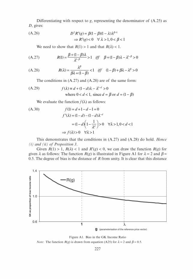
Differentiating with respect to g, representing the denominator of (A.25) asD, gives:

(A.26)

We need to show that R(1) > 1 and that R(l) < 1.

(A.27)

(A.28)

The conditions in (A.27) and (A.28) are of the same form:

(A.29)

We evaluate the function f (l) as follows:

This demonstrates that the conditions in (A.27) and (A.28) do hold. Hence

(i) and (ii) of Proposition 3.Given R(1) > 1, R(l) < 1 and R¢(g) < 0, we can draw the function R(g) for

given l as follows: The function R(g) is illustrated in Figure A1 for l = 2 and b =0.5. The degree of bias is the distance of R from unity. It is clear that this distance

f d d

f d d

d d

f

d

d

1 1 1 0

1 1

1 11

0 1 0 1

0 1

( ) = + - - =¢( ) = -( ) - -( )

= -( ) -ÊË

ˆ¯ > " > < <

fi ( ) > " >

-l l

ll

l l

,

f d d

d d d

dl l lb b

( ) ∫ + -( ) - >< < = = -( )

-1 0

0 1 1

1

where since or ,

R iffll

bl bb bl l

bb( ) =

+ -( )< -( ) + - >

11 1 0

R iff11

1 1 011( ) =

+ -( )> + -( ) - >-

-b b ll

b b l lbb

D R g

R g

2 11 1

0 1 0 1

¢( ) = -( ) -( )

fi ¢( ) < " > < <

-b b l ll b

b

,

227

0.6

1.0

1.4

0 2 3

g (parameterisation of the reference price vector)

GK

as

pro

po

rtio

n o

f tr

ue

inco

me

rati

o

R(g)

l1

Figure A1. Bias in the GK Income Ratio

Note: The function R(g) is drawn from equation (A25) for l = 2 and b = 0.5.

(A.30)

increases either as g is larger than l, or as g becomes smaller than 1. Hence part

(iii) of Proposition 3.Finally, for a given value of g, we can differentiate the expression in (A.25)

with respect to l:

If g is greater than l, as postulated in part (i), R is less than unity and decreas-ing in l. Thus the magnitude of the (downward) bias is increasing in l. If g is lessthan unity, as postulated in (ii), then l is greater than g and R is greater than unityand increasing in l. Thus the magnitude of the (upward) bias is increasing in l.Hence part (iv) of Proposition 3.

References

Ackland, Robert, Steve Dowrick, and Benoit Freyens, “Measuring Global Poverty: Why PPP MethodsMatter,” Annual Conference of the International Association for Research into Income and Wealth,Cork, Ireland, 2004.

Afriat, S. N., “The True Index,” in A. Ingham and A. M. Ulph (eds), Demand, Equilibrium, and Trade:Essays in Honor of Ivor F. Pearce, Macmillan, New York, 37–56, 1984.

Atkinson, Anthony B. and Andrea Brandolini, “Promise and Pitfalls in the Use of ‘Secondary’ Data-Sets: Income Inequality in OECD Countries as a Case Study,” Journal of Economic Literature,39(3), 771–99, 2001.

Balassa, B., “The Purchasing Power Parity Doctrine: A Reappraisal,” Journal of Political Economy,72(6), 584–96, 1964.

Bergstrand, Jeffrey H, “Structural Determinants of Real Exchange Rates and National Price Levels:Some Empirical Evidence,” American Economic Review, 81, 325–34, 1991.

Berry, Albert, François Bourguignon, and Christian Morrisson, “Changes in the World Distributionof Income between 1950 and 1977,” Economic Journal, 93(37), 331–50, 1983.

Bhagwati, Jagdish, “Why Are Services Cheaper in the Poor Countries,” Economic Journal, 94, 279–86,1984.

Bourguignon, François and Christian Morrisson “Inequality Among World Citizens: 1820–1992,”American Economic Review, 92(4), 727–44, 2002.

Chotikapanich, Duangkamon, “A Comparison of Alternative Functional Forms for the LorenzCurve,” Economics Letters, 41(2), 129–38, 1993.

Chotikapanich, Duangkamon, Rebecca Valenzuela, and D. S. Prasada Rao, “Global and RegionalInequality in the Distribution of Income: Estimation with Limited and Incomplete Data,” Empir-ical Economics, 22(4), 533–46, 1997.

Deininger, Klaus and Lyn Squire, “A New Data Set Measuring Income Inequality,” World Bank Eco-nomic Review, 10(3), 565–91, 1996.

Diewert, Erwin, “Similarity and Dissimilarity Indexes: An Axiomatic Approach,” University of BritishColumbia Discussion Paper, 02–10, 2002.

Dowrick, Steve and John Quiggin, “True Measures of GDP and Convergence,” American EconomicReview, 87(1), 41–64, 1997.

Falvey, Rodney E. and Norman Gemmell, “A Formalisation and Test of the Factor Productivity Expla-nation of International Differences in Service Prices,” International Economic Review, 37(1),85–102, 1996.

Firebaugh, Glenn, “Empirics of World Income Inequality,” American Journal of Sociology, 104(6),1597–630, 1999.

Gerschenkron, Alexander, A Dollar Index of Soviet Machinery Output, 1927–28 to 1937, Rand Corporation, Santa Monica, CA, 1951.

Grosh, Margaret-E. and E. Wayne Nafziger, “The Computation of World Income Distribution,”Economic Development and Cultural Change, 34(2), 347–59, 1986.

b b∂ l

∂lb b l

l∂ l

∂ll

bgR g g

R gas g

+ -( )[ ]( )

=-( ) -( )

fi( )

>=< >=<

-11

0

1

;

;

228

(A.31)

Hill, Robert J., “Measuring Substitution Bias in International Comparisons Based on Additive Purchasing Power Parity Methods,” European Economic Review, 44(1), 145–62, 2000.

Korzeniewicz, Roberto Patricio and Timothy Patrick Moran, “World Economic Trends in the Distribution of Income, 1965–92,” American Journal of Sociology, 102(4), 1000–39, 1997.

Kravis, Irving B., Alan Heston, and Robert Summers, World Product and Income: International Com-parisons of Real Gross Products, The Johns Hopkins University Press, Baltimore, 1982.

Li, Hongyi, Lyn Squire, and Heng-fu Zou, “Explaining International and Intertemporal Variations inIncome Inequality,” Economic Journal, 108(446), 26–43, 1998.

Maddison, Angus, Monitoring the World Economy: 1820–1992, Organization for Economic Co-oper-ation and Development, Paris and Washington, D.C., 1995.

Melchior, Arne, Kjetil Telle, and Henrik Wiig, Globalisation and Inequality: World Income Distributionand Living Standards, 1960–98. Studies on Foreign Policy Issues, Report 6B, Royal NorwegianMinistry of Foreign Affairs, Oslo, Norway, 1–42, 2000.

Milanovic, Branko, “True World Income Distribution, 1988 and 1993: First Calculations Based onHousehold Surveys Alone,” Economic Journal, 112(476), 51–92, 2002.

Nuxoll, Daniel A., “Differences in Relative Prices and International Differences in Growth Rates,”American Economic Review, 84(5), 1423–36, 1994.

Sala-i-Martin, Xavier, “The World Distribution of Income (Estimated from Individual Country Dis-tributions),” NBER Working Papers: 8933, National Bureau of Economic Research, Inc., 2002a.

———, “The Disturbing ‘Rise’ of Global Income Inequality,” NBER Working Paper, 8904, 1–72,2002b.

Samuelson, Paul, “Theoretical Notes on Trade Problems,” Review of Economics and Statistics, 46(2),145–54, 1964.

———, “Analytical Notes on International Real-Income Measures,” Economic Journal, 84(335),595–608, 1974.

Schulz, T. Paul, “Inequality in the Distribution of Personal Income in the World: How it is Changingand Why,” Journal of Population Economics, 11, 307–44, 1998.

Summers, Robert and Alan Heston, “The Penn World Table (Mark 5): An Expanded Set of Interna-tional Comparisons, 1950–1988,” Quarterly Journal of Economics, 106(2), 327–68, 1991.

Theil, Henry, “World Income Inequality,” Economics Letters, 2(1), 99–102, 1979.———, Studies in Global Econometrics, Kluwer Academic Publishers, Amsterdam, 1996.Theil, Henry and James L. Seale, “The Geographic Distribution of World Income, 1950–90,” De

Economist, 4, 1994.UNDP, Human Development Report 1999, Oxford University Press, New York, 1999.Varian, Hal R., “Non-Parametric Tests of Consumer Behaviour,” Review of Economic Studies, 50(1),

99–110, 1983.World Bank, Purchasing Power of Currencies: Comparing National Incomes Using ICP Data, Interna-

tional Economics Department, World Bank, Washington, D.C., 1993.———, “ICP Regional Datasets for 1993,” supplied to authors by the Bank’s international compari-

son section, 2000.———, “Global Development Network Database: Macro Time Series,” http://www.worldbank.

org/research/growth/GDNdata.htm, 2001.

229