Contour Connection Method for Automated Identification and Classification of Landslide Deposits

Ben A. Leshchinskya, Michael J. Olsenb and Burak F. Tanyuc aAssistant Professor, Corresponding Author, Oregon State University, Dept. of Forest Eng., Res. And Mgmt., 273 Peavy Hall, Corvallis, OR 97331, ben.leshchinsky@oregonstate.edu, +1-541-737-887 bAssistant Professor, Oregon State University, Dept. of Civil and Constr. Eng., 313 Owen Hall, Corvallis, OR 97331, michael.olsen@oregonstate.edu cAssistant Professor, George Mason University, Dept. of Civil, Env. and Infrastructural Eng., 1409 Nguyen Engineering Building, Corvallis, Fairfax, VA 22030, btanyu@gmu.edu Abstract

Landslides are a common hazard worldwide that result in major economic, environmental and social impacts. Despite their devastating effects, inventorying existing landslides, often the regions at highest risk of reoccurrence, is challenging, time-consuming, and expensive. Current landslide mapping techniques include field inventorying, photogrammetric approaches, and use of bare-earth (BE) lidar digital terrain models (DTMs) to highlight regions of instability. However, many techniques do not have sufficient resolution, detail, and accuracy for mapping across landscape scale with the exception of using BE DTMs, which can reveal the landscape beneath vegetation and other obstructions, highlighting landslide features, including scarps, deposits, fans and more. Current approaches to landslide inventorying with lidar to create BE DTMs include manual digitizing, statistical or machine learning approaches, and use of alternate sensors (e.g., hyperspectral imaging) with lidar.

This paper outlines a novel algorithm to automatically and consistently detect landslide deposits on a landscape scale. The proposed method is named as the Contour Connection Method (CCM) and is primarily based on bare earth lidar data requiring minimal user input such as the landslide scarp and deposit gradients. The CCM algorithm functions by applying contours and nodes to a map, and using vectors connecting the nodes to evaluate gradient and associated landslide features based on the user defined input criteria. Furthermore, in addition to the detection capabilities, CCM also provides an opportunity to be potentially used to classify different landscape features. This is possible because each landslide feature has a distinct set of metadata – specifically, density of connection vectors on each contour – that provides a unique signature for each landslide. In this paper, demonstrations of using CCM are presented by applying the algorithm to the region surrounding the Oso landslide in Washington (March 2014), as well as two 14,000 hectare DTMs in Oregon, which were used as a comparison of CCM and manually delineated landslide deposits. The results show the capability of the CCM with limited data requirements and the agreement with manual delineation but achieving the results at a much faster time.

1.1 Introduction

A landslide, as defined by Cruden (1991) is a movement of a mass of rock, debris, or earth down a slope. This geo-hazard can result in severe consequences, including economic and infrastructural impacts and casualties, in the worst cases. Therefore, identifying hazardous locations, determining the magnitude of risk, understanding causative factors, and mitigating the impacts of this phenomenon have been a critical area of research. Typically, previous studies focus on evaluating the specific details of individual landslides and understanding the causative mechanism. Beyond these case studies, large inventories of landslides are being collected by geologists and remote sensing professionals in an effort to mitigate landslide impacts. For example, the United States Geological Survey (USGS) has an open access database on their web site reporting the landslides that occur around the world since 1994 (USGS, 2014) as well as other state and local organizations also work on establishing hazard databases (e.g., Burns et. al. 2011 and Puget Sound lidar Consortium, 2014).

Landslides manifest in a variety of morphologies and magnitudes (Burns and Madin, 2009). For example, recently in March and April in 2014, the media has reported several landslide events that ranged significantly in magnitude and location. The first major landslide reported was in Steelhead Haven, 6.5 kilometers east of Oso, Washington (The Pacific Northwest of the United States). The footprint of the landslide covered an area approximately 2.6 square kilometers and 41 people have lost their lives (Seattle Times, 2014). At the end of April, a large landslide in Afghanistan’s Badakhshan region covered about 300 homes with mud and debris and more than 350 people reported to have lost their lives with an additional 2,000 people missing (BBC, 2014). In general, the combination of geometry of the slope/hillside, vegetation, soil and rock properties, rock mass structure, precipitation and water conditions (including both groundwater and surface water) have direct effects affecting slope instability (Cornforth, 2005; Ling et al. 2009; Leshchinsky 2013). Understanding these factors enables scientists and engineers to evaluate potential hazards for particular areas, a critical step for prevention or minimization of damage. However, geotechnical evaluation of slope stability is often on an individual basis, and often only in consideration of two-dimensional conditions (ignoring three-dimensional effects) with idealized soil and rock properties. DTM-based mechanistic are mainly dependent on the infinite slope method (translational failure with assumed soil strength) for highlighting regions of instability (Deitrich et al. 2001). Currently, the USGS has a specific landslide hazards program that includes seven monitoring sites along the west coast where particular landslides are monitored with an aim on developing methodologies geared towards predicting the behavior of the landslide (USGS, 2014). A similar interest in characterizing and mitigating of landslides also exist within the transportation agencies in the United States. The Transportation Research Board has developed a special report particularly focusing on landslide investigations and mitigations (Turner and Schuster, 1996) and more recently National Research Council (NRC) has developed guidelines for assessment of national landslide and rock fall hazards (NRC, 2004). Mitigation of landslides is a benefit for a variety of reasons, including safety and development of

infrastructure and environmental concerns, yet the most ideal way of mitigating the impacts of landslides is simple – avoiding them. However, avoidance of these features is not trivial as it requires adequate mapping and inventorying – a daunting task over large, vegetated landscapes. 1.1.1 Landslide Mapping

Despite its challenges, landslide hazard mapping is a common practice in urban settings for planning purposes. There are three primary types of mapping:

1. Inventory – Mapping, classification and documentation of existing landslides, both historic and pre-historic based on geologic evidence,

2. Susceptibility – Mapping based on soil and site conditions that indicate areas susceptible to landslides, and;

3. Hazard – Mapping and evaluating the potential for damage, incorporating external factors. This differs from susceptibility in that the triggering sources are included in the analysis. In some literature, these are referred to generically as hazard maps. Further, potential mapping methodologies can be classified into deterministic and probabilistic.

Recently, there has been a drive to utilize new remote sensing technologies to identify, investigate, and map landslides as opposed to field visits (small coverage) or classical photogrammetry (susceptible to missing landslides in forested terrain). Several techniques include (but are not limited to) differential interferometric synthetic aperture radar (DInSAR) which can measure displacements (Belardinelli et al., 2005) at high (mm-level) accuracies, panchromatic QuickBird satellite images of the ground that can be used to evaluate changes in topography (Niebergall et al., 2007), airborne and terrestrial geodetic lidar-scans, which can create detailed, 3D point clouds used for monitoring changes in the terrain (Jaboyedoff et al., 2012; Olsen et al., 2012; Olsen, 2014; Conner and Olsen, 2014) at high resolutions, and unmanned aerial vehicles (UAVs) equipped with digital cameras to map and record spatial and temporal measurements (Niethammer et al., 2012).

Using remote sensing methods provide a significant advantage by facilitating landscape-scale hazard inventories without the practical challenges of physically verifying landslide features (Van Westen et al. 2008, Burns and Madin, 2009). Not only does the use of some new remote sensing technologies enable landscape-scale collection of topography; but also it can provide abilities to remove vegetation or forest canopies from the models, clearly exposing the scarred earth beneath. However, when data obtained from remote sensing is used to develop models to predict and forecast landslides, the models become very complex; therefore, inventorying of old landslides is the first major, yet exhaustive measure to evaluate potential hazards on a landscape.

1.1.2 Use of lidar in Remote Sensing

Light detection and ranging (lidar) technology is a line-of-sight technology that emits laser pulses at defined, horizontal and vertical angular increments to produce a 3D point cloud, containing XYZ coordinates for objects that return a portion of the light pulse within range of the sensor. This detailed point cloud is a virtual world that can be explored and analyzed for multiple uses long after the data are collected. Time series surveys enable damage and deterioration analyses at unprecedented detail across multiple scales. Currently, an initiative, the 3D elevation plan (3DEP) is underway to obtain airborne lidar data across the entire U.S. at meter level resolution (Snyder, 2012).

One of the key benefits of lidar data is its ability to model the ground surface and key geomorphological features covered by vegetation when a portion of the emitted light is able to penetrate the ground. A variety of processing techniques exist to filter ground points and create a Digital Terrain Model (DTM). These approaches depend on the type of terrain and vegetation characteristics. Common approaches including lowest elevations, ground surface steepness, ground surface elevation difference, and ground surface homogeneity are reviewed in Meng et al. (2010).

In the last decade, lidar has become a key tool for landslide delineation. Jaboyedoff et al. (2012) provides a detailed review of lidar usage for landslide studies. Lidar has been used to undertake detailed geological assessments of several landslides, enabling improved understanding of the processes and mechanisms contributing to landslide movement. Considerable work has also been undertaken in recent years to document the patterns of landslides and mechanisms for failure, particularly in forested environments where lidar provides detailed surface topography to delineate landslides that were previously undetectable. In general, there are three approaches to delineate landslides from lidar data:

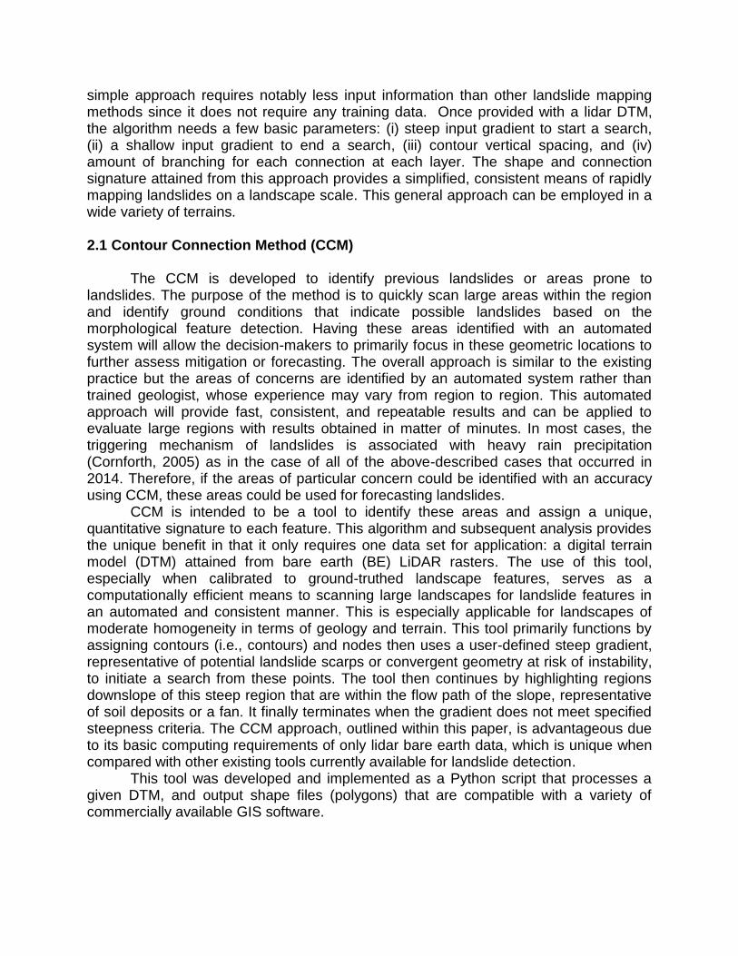
1. Manual – Manually delineating landslide deposits and scarps from airborne lidar

is the most common approach (see Figure 1). Burns and Madin (2009) demonstrate a systematic methodology using airborne lidar to map landslides in northwest Oregon, ultimately creating landslide hazard maps that could be used by local government for planning purposes. Similarly, Schulz (2007) presents approaches for landslide susceptibility estimation from airborne lidar data.

2. Statistical\Machine Learning – Mora et al. (2014) developed an approach using

repeat scans to probabilistically determine areas that are likely susceptible to future landslides or are undergoing movement. Booth et al (2009) analyzed topographic signatures (wavelengths) observed in lidar data and used machine learning to automatically identify deep-seated landslides. This approach utilized power spectra and two-dimensional Fourier transforms to characterize and calibrate landslide morphology, facilitating algorithmic landslide searches in their five study areas. The approach is calibrated by using a landslide inventory in a nearby area.

3. Combination with another sensor - Wang et al. (2013) performed landslide boundary delineation using a combination of terrestrial and airborne lidar.

Figure 1. Comparison of ortho-photograph, lidar bare earth hillshade and landslide

deposit inventory (Burns et. al, 2013).

Although automated landslide detection systems are available, their accuracy is directly related to the resolution and qualities of the input data, requiring expensive datasets that are often beyond the reach of decision-makers affiliated with mission agencies concerned with addressing landslide hazards. Many systems are also computationally expensive, requiring significant post-processing with a steep learning curve. Therefore, using and understanding these complex models require specialty training and their accuracy of predictions have not been sufficient enough for public agencies to invest the time and resources to have a sufficient number of trained professionals in each region. Currently, geologists in most regions frequently use site investigation, topographic maps, known geology, and known historic landslides to identify the potential areas of concern. This method, although if performed by a trained geologist with expertise, may provide results with sufficient accuracy, requires substantial time and effort, and ultimately, the result is subjective because it is based on the interpretation of an individual. This also leads to inconsistencies between mapped tiles.

An alternative to this approach is presented herein, called the Contour Connection Method (CCM). This approach operates on downsampled lidar bare earth (BE) DTMs and uses discretized contours (i.e., contours) and vector connections to serve as mediums for shape and steepness between layers. A potential landslide deposit is designated from steep scarp geometry from vector connections and is terminated when landslide deposits have shallow vector connections. Therefore, this

simple approach requires notably less input information than other landslide mapping methods since it does not require any training data. Once provided with a lidar DTM, the algorithm needs a few basic parameters: (i) steep input gradient to start a search, (ii) a shallow input gradient to end a search, (iii) contour vertical spacing, and (iv) amount of branching for each connection at each layer. The shape and connection signature attained from this approach provides a simplified, consistent means of rapidly mapping landslides on a landscape scale. This general approach can be employed in a wide variety of terrains.

2.1 Contour Connection Method (CCM)

The CCM is developed to identify previous landslides or areas prone to landslides. The purpose of the method is to quickly scan large areas within the region and identify ground conditions that indicate possible landslides based on the morphological feature detection. Having these areas identified with an automated system will allow the decision-makers to primarily focus in these geometric locations to further assess mitigation or forecasting. The overall approach is similar to the existing practice but the areas of concerns are identified by an automated system rather than trained geologist, whose experience may vary from region to region. This automated approach will provide fast, consistent, and repeatable results and can be applied to evaluate large regions with results obtained in matter of minutes. In most cases, the triggering mechanism of landslides is associated with heavy rain precipitation (Cornforth, 2005) as in the case of all of the above-described cases that occurred in 2014. Therefore, if the areas of particular concern could be identified with an accuracy using CCM, these areas could be used for forecasting landslides.

CCM is intended to be a tool to identify these areas and assign a unique, quantitative signature to each feature. This algorithm and subsequent analysis provides the unique benefit in that it only requires one data set for application: a digital terrain model (DTM) attained from bare earth (BE) LiDAR rasters. The use of this tool, especially when calibrated to ground-truthed landscape features, serves as a computationally efficient means to scanning large landscapes for landslide features in an automated and consistent manner. This is especially applicable for landscapes of moderate homogeneity in terms of geology and terrain. This tool primarily functions by assigning contours (i.e., contours) and nodes then uses a user-defined steep gradient, representative of potential landslide scarps or convergent geometry at risk of instability, to initiate a search from these points. The tool then continues by highlighting regions downslope of this steep region that are within the flow path of the slope, representative of soil deposits or a fan. It finally terminates when the gradient does not meet specified steepness criteria. The CCM approach, outlined within this paper, is advantageous due to its basic computing requirements of only lidar bare earth data, which is unique when compared with other existing tools currently available for landslide detection. This tool was developed and implemented as a Python script that processes a given DTM, and output shape files (polygons) that are compatible with a variety of commercially available GIS software.

2.1.1 Automated Landslide Detection Algorithm: Overview

Given scarp gradient input parameters, nodal connections within a predefined range are considered at start of analysis, starting at contour with highest elevation. Then, every connection from the nodes activated by detection of a scarp feature, according to input data will begin a branch of connections that are directly or indirectly connected to the nodes that were activated by scarp features. This chain of nodal connections branching from these initial “activation points” will highlight a general shape and “flow path” of landslide deposits based on input data calibrated to existing landslide lidar DTMs. Landslide features that may be detected using CCM include slope failures and downslope deposits that have a headscarp or headwall feature (i.e. a steeper portion at the initiation point of a slope failure), primarily focusing initial application on translational slides, rotational failures, earth flows, debris flows, and topples. 3.1 Automated Landslide Detection Algorithm: General Numerical Approach

The automated detection of landslides begins with the input of lidar DTMs, which consists of a series of X, Y, and Z coordinates necessary to perform a topographical analysis of the landscape without vegetation or canopy cover. A search area within a given DTM must be input to bracket the boundaries of an automated landslide search. Within a search area, the following input parameters will be used to govern detection of a potential active landslide zone using a lidar DTM:

(Xo, Yo, Zo), a search area with a given length, width and height in the X, Y and Z (Cartesian) coordinate system;

scarp, a minimum gradient for scarp classification;

active, a minimum gradient for active slide region;

Ez, a fixed vertical distance between X-Y contour layers for given range Z;

E, a tolerance for finding points for each contour layer;

Ln, a fixed length between contour node assignments; and,

Bn, a branching connection parameter.

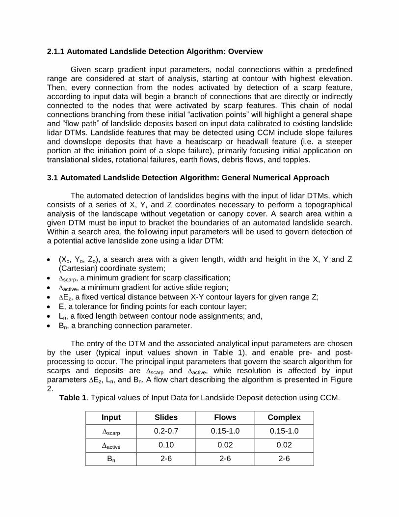
The entry of the DTM and the associated analytical input parameters are chosen by the user (typical input values shown in Table 1), and enable pre- and post-processing to occur. The principal input parameters that govern the search algorithm for scarps and deposits are scarp and active, while resolution is affected by input parameters Ez, Ln, and Bn. A flow chart describing the algorithm is presented in Figure 2.

Table 1. Typical values of Input Data for Landslide Deposit detection using CCM.

Input Slides Flows Complex

scarp 0.2-0.7 0.15-1.0 0.15-1.0

active 0.10 0.02 0.02

Bn 2-6 2-6 2-6

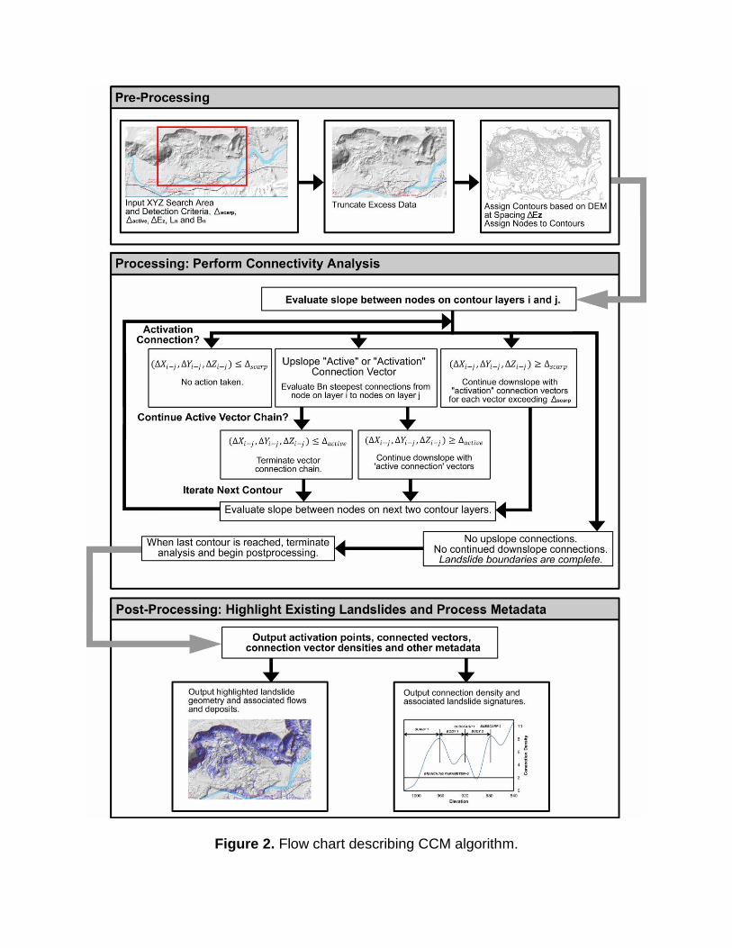
Figure 2. Flow chart describing CCM algorithm.

Preprocessing of the DTM is facilitated by the assignment of contour layers and connectivity between pre-assigned, evenly spaced nodes on each contour (Figure 3). Within a search area (X, Y, Z) and (X+L, Y+W, Z+H), contours are assigned based on

the coordinates from a recorded bare DTM, and the contour interval input, Ez. Starting at the point of maximum elevation of the search area, contours are assigned based on coordinates that fall within each respective elevation. Coordinates (Xi,Yi,Zi) are added to each respective contour, Zi.

At each contour, a pre-selected, even spacing of nodes will be assigned. The assignment of nodes begins at the lowest (X, Y, Zi) coordinate and assigns each progressive node at a spacing (Ln) along a contour. This assignment of nodes is performed consistently for each contour layer until the lower threshold of the search elevation is reached.

With the discretization pre-processing phase finished, the processing phase begins. The assignment of nodes at specified lateral and vertical spacing facilitates the processing step, which includes detection of landslide features based on the search

criteria of scarp gradient, scarp, active slide zone gradient, and branching parameters (Figure 2). This begins between the top contour, Zi, and next contour at a lower elevation, Zj. These contours are described as:

𝑍𝑖 = 𝐸𝑙𝑒𝑣𝑎𝑡𝑖𝑜𝑛 𝑎𝑡 𝑐𝑜𝑢𝑛𝑡𝑜𝑢𝑟 𝑖

𝑍𝑗 = 𝐸𝑙𝑒𝑣𝑎𝑡𝑖𝑜𝑛 𝑎𝑡 𝑐𝑜𝑢𝑛𝑡𝑜𝑢𝑟 𝑗 = 𝑍𝑖 − ∆𝐸𝑍

𝑁𝑜𝑑𝑒𝑠 𝑖𝑛 𝐿𝑎𝑦𝑒𝑟 𝑍𝑖 = (𝑋𝑖1, 𝑌𝑖1), (𝑋𝑖2, 𝑌𝑖2), … , (𝑋𝑖𝑛, 𝑌𝑖𝑛)

𝑁𝑜𝑑𝑒𝑠 𝑖𝑛 𝐿𝑎𝑦𝑒𝑟 𝑍𝑗 = (𝑋𝑗1, 𝑌𝑗1), (𝑋𝑗2, 𝑌𝑗2), … , (𝑋𝑗𝑛, 𝑌𝑗𝑛)

The gradient between each node on Zi is evaluated to each node on Zj. When

connections are made between nodes that are equal to or exceed a gradient indicative of scarp signature, the node on Zi is considered an activation node, the node on Zj is considered an active node, and the connection between these points is called an activation connection vector (see Figure 2). This process is performed using linear optimization between two consecutive contour layers and their respective nodes, described by:

(∆𝑋𝑖−𝑗, ∆𝑌𝑖−𝑗, ∆𝑍𝑖−𝑗) ≥ ∆𝑠𝑐𝑎𝑟𝑝

An activation node indicates that one or more optimized maximum gradient

connections stemming from that node are activation connection vectors, and downslope nodes that are connected to these nodes are active. The active nodes that are downslope of the activation connection vector then connect to the next n closest nodes downslope of it, known as active connection vectors (see Figure 3). The quantity of active connection vectors that originate from each active node is equal to the branching parameter, Bn. Active connection vectors may or may not have a larger slope than

scarp, but continue branching downslope until the gradient of the active connection

vectors becomes less than active. When the slope for a connection vector between two

contours becomes less than active, the active nodes terminate at this point. At any contour, nodes lying in between the outer most nodes at the boundary of a single active landslide zone are considered an active node, even if no connection vectors are in

contact with it (see Figure 3). This behavior is common when the flow path of the landslide is circumventing an obstacle or the fan or toe deposit begins. These unconnected nodes within the flow path are called orphan nodes. The calculation of contours, activation nodes, active nodes, orphan nodes, active connection vectors, and the active landslide zone constitutes the processing phase of the CCM, which can then be post-processed into meaningful data based on the flow chart shown on Figure 2.

Figure 3. Conceptual schematic of active landslide zone (Bn=2).

The density of connection vectors between layers is indicative of morphological features within a slide. Connection vector density, Di, is defined by the number of upslope connection vectors connecting to active nodes on a contour layer (see Figures 3 and 4). Contours containing nodes with multiple upslope connections are indicative of steep concavities; while areas with orphan nodes are indicative of outward flow and more shallow convexities. For example, a vector direction that is shaped concavely inwards and has notably steep grades may be indicative of a scarp signature or the body of a landslide that has occurred, typically represented by connection vector densities that are greater than the branching parameter, Bn. Inversely, outward vector flow or shallow vector gradient as elevation contours may be indicative of a landslide fan, or deposits from an earth flow and manifest as connection vector densities that are less than Bn (Figure 3). The calculation of active connection density is used to as a quantifiable and unique signature or “fingerprint” for given landslide topology.

Figure 4. Morphological signature for landscape feature (based on slide schematic in

figure 3, Bn=2). Progressive change in the connection vector density with a shift in elevation is indicative of unique features in the morphological signature of a landslide. Connection vector density is higher when more upslope connection vectors are connecting to the active nodes in an elevation level. Inversely, the connection density is lower when fewer upslope connection vectors are connecting to active nodes, or more orphan nodes are starting to be introduced on an elevation level (see Figure 4). This higher density of

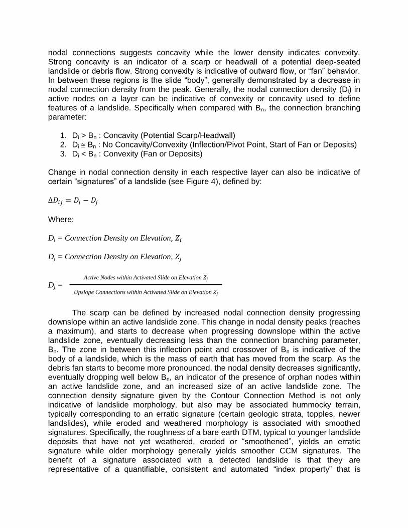
nodal connections suggests concavity while the lower density indicates convexity. Strong concavity is an indicator of a scarp or headwall of a potential deep-seated landslide or debris flow. Strong convexity is indicative of outward flow, or “fan” behavior. In between these regions is the slide “body”, generally demonstrated by a decrease in nodal connection density from the peak. Generally, the nodal connection density (Di) in active nodes on a layer can be indicative of convexity or concavity used to define features of a landslide. Specifically when compared with Bn, the connection branching parameter:

1. Di > Bn : Concavity (Potential Scarp/Headwall) 2. Di Bn : No Concavity/Convexity (Inflection/Pivot Point, Start of Fan or Deposits) 3. Di < Bn : Convexity (Fan or Deposits)

Change in nodal connection density in each respective layer can also be indicative of certain “signatures” of a landslide (see Figure 4), defined by: ∆𝐷𝑖𝑗 = 𝐷𝑖 − 𝐷𝑗

Where: Di = Connection Density on Elevation, 𝑍𝑖 Dj = Connection Density on Elevation, 𝑍𝑗

Dj =

The scarp can be defined by increased nodal connection density progressing

downslope within an active landslide zone. This change in nodal density peaks (reaches a maximum), and starts to decrease when progressing downslope within the active landslide zone, eventually decreasing less than the connection branching parameter, Bn. The zone in between this inflection point and crossover of Bn is indicative of the body of a landslide, which is the mass of earth that has moved from the scarp. As the debris fan starts to become more pronounced, the nodal density decreases significantly, eventually dropping well below Bn, an indicator of the presence of orphan nodes within an active landslide zone, and an increased size of an active landslide zone. The connection density signature given by the Contour Connection Method is not only indicative of landslide morphology, but also may be associated hummocky terrain, typically corresponding to an erratic signature (certain geologic strata, topples, newer landslides), while eroded and weathered morphology is associated with smoothed signatures. Specifically, the roughness of a bare earth DTM, typical to younger landslide deposits that have not yet weathered, eroded or “smoothened”, yields an erratic signature while older morphology generally yields smoother CCM signatures. The benefit of a signature associated with a detected landslide is that they are representative of a quantifiable, consistent and automated “index property” that is

Active Nodes within Activated Slide on Elevation 𝑍𝑗

Upslope Connections within Activated Slide on Elevation 𝑍𝑗

unique to that specific landscape feature - a property that may then be associated with other significant behaviors associated with landslide morphology, such as erosion potential, probabilistic analyses, risk and more.

A user’s selection of input parameters can slightly influence the analysis results. One node at contour elevation Z1 can only connect to Bn node(s) at contour elevation Z2 (elevation below Z1), and the connection must be indicative of the shortest route (i.e., steepest). Hence, selected nodal density and contour density are important for discretization and accuracy. Higher quantities of both enable better discretization, and potentially more refined landslide detection output, however, the coarser the results, the more tolerance is required for DTM noise (i.e., stumps, boulders, trees, etc.). The shortest distance detected between each of the discretized nodes and elevations is a simple linear optimization problem with limited computing requirements, especially since analysis begins from the top elevation contour and only considers nodal connections between the next, highest elevation below the starting contour. Hence, only two contours are being analyzed at a time. However, it is key that the user is consistent with input parameters when searching for specific landslide features across a landscape. For

example, certain input parameters (i.e., scarp, active) will highlight morphological features that are typically susceptible to debris flows (i.e., headwalls, the cirque features of a channel or gully found in mountainous terrain), while other parameters will highlight the features indicative of deep-seated landslides (scarps, fan deposits). Contour interval and node spacing should typically be at least greater than three times the DTM pixel dimensions to prevent artifacts in the analysis. Therefore, if available, it is beneficial to choose input parameters that have a basis on ground-truthed landslides or known areas of instability and then use it to search landscapes with similar geology and terrain. However, a range of typical input values is presented in Table 1, which may serve as initial input if data is unavailable. If ground-truthed data or known landslides are not available, it is recommended that the user run the analysis with both the upper bound

and lower bound values for scarp to highlight landslide geometry. If landslide features are being detected according to user judgment, then correct input values are being used. General ranges of input parameters for three different common landslide features (slides, flows, and complex movements) are provided in Table 1. One practical consideration is that CCM needs a digital terrain model raster with pixels sufficiently small (preferably less than 5m) to adequately resolve the small landslide features of interest. As with any technique (manual or automatic), too large of a pixel size will not enable the detection of smaller slides. Larger nodal spacing and vertical contour spacing will reduce the discretization of details attained from a DTM; however, there will be more tolerance for noise resulting from features such as vegetation or boulders. Contour interval (contour spacing) is the primary factor in the filtration of noise or the resolution of details. Contour interval should be chosen to ensure that it is smaller than the size of typical expected scarp features. For example, if scarp features in a region tend to be between 5 and 15 meters in height, the user should select a maximum contour interval of 5 meters as to ensure smaller scarps are not neglected in the search. If a larger contour interval is chosen, it is possible that smaller scarps will not be detected because the steepness is not adequately discretized. Hence, refined accuracy can be attained with some basic pre-defined knowledge of regional instability. It is suggested that the spacing for nodes, Ln, is generally less than or equal to the contour

interval between layers, Ez to ensure that the flow path will be adequately resolved. Furthermore, the nodal spacing, assigned by the algorithm, needs to be greater than the cell size of the baseline DTM. Nodal spacing, applied along the true distance of a contour (which can be affected by DTM resolution/pixel size) is best kept at spacing closer to the contour interval for computational efficiency. Finally, increasing the branching parameter increases the size and shading of the detected regions. Input of larger Bn value results in a larger shaded area as it connects to an increasing amount of nodes in the following layer; however, it also increases computation time in a non-linear rate. This factor, like nodal density, can be used to discretize landslide deposits as well as amplify output signatures (see section 4.1.4). A user may choose to perform several iterations of an analysis to observe the effects of branching parameters, which are typically adequate when kept between 2 and 6 (see table 1), but the effects of Bn primarily affect visualization and post-processing (landslide signature amplification). Activation nodes or active nodes are automatically calculated based on the aforementioned input parameters. Calibration of the CCM approach to large landscapes that are adequately homogenous in terrain and geology will provide the best results. That is, appropriate input parameters based on size and geometry of a number of known landslides with varying shape, classification and size will allow for better bounding of input criteria and more refined detection accuracy. 4.1 Results

4.1.1 Case 1: Oso Landslide and Surrounding Region, Snohomish County, Washington

On March 22nd, 2014, a catastrophic landslide occurred above the town of Oso, Washington, resulting in the tragic loss of human lives; however, the landscape surrounding Oso and the Stillaguamish River is far from static. Despite ubiquitous landslide features readily apparent in the bare earth lidar DTM (1 meter pixel dimension, Figure 5), the satellite imagery shows little hint of the surrounding slopes’ unstable history. A landslide inventory by the US Geological Survey (Haugerud, 2014) also contains these landslide deposits, which includes the traits of many slides of varying ages in a region known for slope instability. The landslide inventory, assessed by a trained geologist (Haugerud, 2014), adequately captures ground-proofed slope failures based on the expertise of the individual assessing the area. However, use of the CCM approach (10 meter contour intervals), with appropriate scarp gradient and active gradient criteria (Table 2) of the slides captures the scarps and deposits of these landslides (see Figure 5). The blue, shaded areas are representative of active

connection vectors that have a gradient less than scarp but more than active

(representative of potential landslide deposits). The red, shaded areas represent active connection vectors stemming from activation points (i.e., the gradient is greater than

scarp, representative of steep, risky terrain and/or headscarps). At this relatively high-resolution array of input parameters, over 900 hectares of land was analyzed for landslides within a matter of approximately 9 minutes (run with an Intel Xeon Processor, 3.2 GHz).

Figure 5. CCM detection and bare earth map of landslides surrounding Stillaguamish

Valley.

Table 2. Summary of input data and results for three case studies.

4.1.2 Case 2: Oregon Coast Range – Pittsburg Quadrangle

The CCM algorithm was tested on a USGS quadrangle consisting of approximately 14261 hectares (142.61 square kilometers, 3 meter pixel dimension, 25 meter contour intervals), with input data shown in Table 2, requiring 59 minutes to run when using one processor (Intel Xeon Processor, 3.2 GHz). The steep and mountainous terrain consisted of complex geology and demonstrated significant instability as there were 754 landslides inventoried by DOGAMI (Burns et al., 2011), 221 of which were observed to be within the past 150 years. By assigning 30 m buffers to the results of the active connection vectors as defined by CCM and converting the previous landslide inventory by DOGAMI to rasters, a comparison of inventories could be made. A basic comparison showed a 91% agreement between pixels representative of landslide deposits (Figure 6). Furthermore, more landslide features and gross

Case Study Ez Ln scarp active Bn Comp.

Time

Inventoried

Landslides

Landslide

Agreement

Landslides

Since 1985

Case 1: Oso 10 10 0.7 0.02 4 00:09:05 N/A N/A N/A

Case 2: Pittsburg 25 25 1.0 0.02 4 00:59:13 754 91% 4

Case 3: Dixie Mt. 20 20 0.15 0.02 4 01:29:25 953 30% 4

landslide area was found with CCM. However, approximately 41% of pixels marked by CCM were false positives, while 59% were true negatives for landslide deposits - potentially an artifact of the analysis, such as channels or valleys in the southwest mountain range (see Table 3). It is important to note that although these places were considered false positives, they are likely locations for debris flows, weathering, topples and similar hazards. To evaluate algorithm sensitivity to input parameters, the analysis

was performed with the lower-bound activation gradient (active) value of 0.15 while keeping all other parameters the same. As expected, this led to better detection of landslide deposits, yet also caused more over-prediction. Specifically, 96% of inventoried landslide deposits were picked up by CCM, yet 76% of pixels were marked as false deposits and 24% as true negatives. Therefore, the algorithm is sensitive to the scarp activation criteria, but little gain is made in accuracy, and potentially the inverse, when shallow activation gradients are applied to very steep terrain. Hence, improved accuracy is possible with input parameters attained from confirmed, regional landslide geometry, especially activation and active gradients. When this range is not too broad, (1) the computational tool will run more efficiently and (2) fewer false positives will be detected. Further work involving use of Booleans and input of other data layers (geology, hydrologic features, etc.) will also help reduce false positives, especially with broader input criteria.

Table 3. Error matrix for comparison of CCM and manual landslide inventorying for

Pittsburg and Dixie Mountain quadrangles.

Landslide Not Landslide

Land

slide

% Pixels Marked as a Landslide

by both Manual Inventory and

CCM (True Positive)

% Pixels Marked as a Landslide by

both Manual Inventory but not CCM

(False Negative)

Not

Land

slide

% Pixels Marked as a Landslide

by CCM but not Manual Inventory

(False Positive)

% Pixels not Marked as a Landslide

by both Manual Inventory but not

CCM (True Negative)

Case 2: Oregon Coast Range – Pittsburg Quadrangle

LS NLS

LS 0.91 0.09

NLS 0.41 0.59

Case 3: Oregon Coastal Range – Dixie Mountain Quadrangle

LS NLS

LS 0.30 0.70

NLS 0.11 0.89

Figure 6. Comparison of DOGAMI landslide inventory (translucent red polygons) and

CCM landslide inventory (blue vectors) in the Pittsburg Quadrangle.

4.1.3. Case 3: Oregon Coastal Range – Dixie Mountain Quadrangle

For the third case, the CCM algorithm was tested on a USGS quadrangle (Dixie Mountain) consisting of approximately 13,872 hectares (138.72 square kilometers, 3 meter pixel dimension, 20 meter contour intervals), with input data shown in Table 2,

requiring 89 minutes to run when using one processor (Intel Xeon Processor, 3.2 GHz). The shallow and hummocky terrain demonstrated even more complex landslide inventory than the one presented in Case 2, including 943 landslides inventoried by DOGAMI, 350 of which were observed to be within the past 150 years. The CCM analysis and conversion of DOGAMI inventory were made the same way as in the Case 2 with 30 m buffers. A preliminary comparison identified by the inventory and CCM showed a 30% agreement between pixels representative of landslide deposits (see Table 3). This lower agreement is representative of large, potentially conservative demarcations of deposits in the northern portion of the DTM (see Figure 7). That is, the large area manually inventoried as a complex movement has a large spatial area assigned to it, meaning that pixel-pixel comparisons may show low agreement, despite adequate detection of most significant landslide features. Furthermore, there is potential that some landslides were missed in the manual inventory, but captured in the CCM mapping. However, these deposits and sub-deposits within are still captured with the CCM, despite the dissonance in pixel comparisons. Furthermore, there was an excellent agreement between regions that were not considered landslide deposits between the two analyses. Specifically, 90% of the pixels that were not marked as landslide deposits in DOGAMI’s inventory were also not marked by the CCM method, showing that the method was generally not over-predicting landslide deposits (i.e., few “false positives”). Despite the seemingly poor match of landslide deposit pixels, CCM still captured the general locations of most of the significant deposits in the quad (see Figure 7). A sensitivity analysis for this region using an upper bound activation gradient of 1.0 yielded no landslide deposit detection as the terrain was shallow and the landslide features tended to have gentle slopes. The fact that the landslides were out of the range with the upper-bound search criteria demonstrates that it would be beneficial to have a general idea of local geology, current landslide inventories, and associated properties for a refined analysis. With a small inventory for a given region, the CCM analysis can be applied adequately to assist with landslide hazard mapping.

Figure 7. Comparison of DOGAMI landslide inventory (translucent red polygons) and CCM landslide inventory (blue vectors) in Dixie Mountain Quadrangle.

4.1.4 Connection Density Signatures

In addition to detection of landslide features, the CCM analysis provides a unique signature of each individual landslide feature that can potentially be used as a classification tool for landscape characteristics (i.e., erosion, age classification, etc.). Three example signatures were chosen for observation.

The first was an earthflow found in Case 2 (Pittsburg Quad, OR) that had a well-defined channel shape and little change in concavity and convexity with elevation change. This feature, marked in Figure 6 and shown in Figure 8a and 8b, is represented by a connection density signature (Figure 8a) that tends to hover around the branching parameter as there is little change in convexity, yet small fluctuations are representative of hummocky terrain and smaller channels within the flow (figure 8b).

Figure 8. Signature for earth flow from Pittsburg Quadrangle (branching parameter=4).

The erratic nature of the signature is representative of hummocky terrain. Red connections are representative of scarp geometry, blue of potential deposits. Another example was that of a complex failure in Case 3 (Dixie Mountain Quad,

OR), represented in Figure 9a and 9b by an initial increase connection density from the scarp to the body, with a highly erratic decrease in density as elevation lowered (Figure 9a), representative of outward earth flow and the extremely hummocky, rough terrain associated with complex earth movements (Figure 9b).

Figure 9. Signature for complex in Pittsburg Quadrangle (branching parameter=4). Red

connections are representative of scarp geometry, blue of potential deposits A final example was that of a deep-seated slide that occurred in Washington

County, OR (Figure 10a and 10b). This signature demonstrated an initial increase in connection density above the branching parameter, Bn, then transitioning into a gradual and smooth decrease in connection vector density as the elevation decreased (Figure 10a). This “smooth” signature can highlight older landslide ages, as the “rough” terrain erodes over time, leaving less ponding, channels and hummocky deposits (Figure 10b). This assessment is in agreement with the DOGAMI inventory classification of the feature as a “prehistoric” slide.

Figure 10. Signature for slide in Dixie Mountain Quadrangle (branching parameter=4). Red connections are representative of scarp geometry, blue of potential deposits

The signature provided by CCM can serve as a classification tool and potentially be connected with important landscape features like (1) concavity; (2) convexity; (3) terrain roughness; and (4) landslide types. An increase in connection density tends to correspond to regions of concavity, like a headwall, channel or gully, while a reduction in connection density tends to correspond to increasing convexity, typical to debris fans or talus deposits, all features of progressive, landscape mass wasting. An erratic signature tends to correspond to regions of highly variable convexity or concavity, typical to hummocky, rough terrain. This uneven terrain is typically implicative of young geological age of a feature, as erosive forces typically “smoothen” roughness over a long period. A gradual signature typically corresponds to an older feature in geological time. The consideration of age in signature could be very important for landslide classification, as landslides of certain age classes may be more or less predisposed to reactivation, dependent on geology, terrain and climate. In addition to roughness and concavity or convexity, a given signature of a landslide feature presents an automated means for classifying landslides in a consistent manner. That is, landslides matching general signature shape criteria may be classified as a certain feature (i.e. translational slide, debris flow, etc.), allowing for improved hazard mapping, risk assessment and classification mechanism. The branching factor, Bn, directly affects the magnitudes of connection densities and can be used as a means of amplifying signatures for enhanced classification. That is, increasing Bn allows for more connections and of course, higher connection densities, exaggerating certain features, like hummocky terrain or extreme changes in concavity or convexity. Improved discretization of signatures can also be affected by increasing number of contours or number of nodes (which will not necessarily amplify signatures, but may refine the signature in relation to elevation profile).

5.1 Conclusions The CCM approach presents an alternative means of establishing landslides and their deposits. This method relies on basic lidar data that is becoming increasingly available and is easily adaptable to a variety of landscapes or hazards types. The CCM approach presents several benefits and contributions in addition to current landslide detection tools or manual approaches. Specifically:

Application of CCM requires only simplified input parameters: input for scarp “activation” gradient, active gradient, contour interval, nodal spacing and branching parameter. Typical input values for select features are presented within this paper. However; selection of input criteria is best based off of geometry of actual, regional landslides. Reasonable agreement with actual DTMs demonstrates potential as a landslide deposit detection tool.

CCM does not require additional data sets (hyper-spectral data, RGB photographic color, etc.), machine learning processes, or many parameters to

function. It requires only basic input pertaining to landslide geometry, which can easily be attained from known, regional features.

Automation of this tool is easily performed. The simplicity of input parameters and calibration facilitates easily application to landscape scale landslide detection. Increased range of input parameters, larger landscapes, higher resolution datasets and increased discretization (higher Bn) can lead to increased computational cost primarily based on the time needed to post-process data, yet the primary parameters that govern the algorithm’s search are the activation and active gradient.

The CCM algorithm can handle large lidar datasets because it can analyze discrete portions of the data at a time. The algorithm is fast because it is a simple slope problem that is performed between only two contours at a time, reducing complexity. This facilitates rapid landslide detection on large landscapes, a slow and subjective process with the trained eye of a geologist.

Use of automated landslide detection tools enables enhanced landslide inventorying and classification. Different landslide characteristics (age, size, hummocky features, etc.) and types (debris flow, earth flow, deep-seated slide, etc.) yield varying risks and concerns for safety, development, environmental concerns and more. The CCM algorithm presents an automated and consistent means of detecting different landslide types and their deposits over large landscapes, enabling not only mapping of hazards, but classification of hazards and their associated risks with a signature that is unique to each individual landslide. Current processes that serve this function are limited, slow and expensive.

With the exceedingly rapid development of lidar technology and push to establish

bare earth maps on a large scale, simplified tools like CCM may serve as an excellent means of identifying and classifying landslides.

There are several different approaches that would facilitate improved automated detection of landslides with CCM. First off, computational speed could easily be improved with parallelization of computations. Furthermore, input parameters could be connected to geology, allowing for improved assessment over regions of inhomogeneous geologic features. Specifically, activation and active parameters could be connected to specific geological formations, reducing user input parameters required for analysis. Finally, use of stream or river channels and computational buffering could allow for over-prediction of landslide deposits in river channels or valleys (i.e. Boolean approach). Despite the propensity of these regions to debris flows, it would enable better segregation of landslide features. Association of CCM with weather data would also allow for better evaluation of precipitation-induced landslide risk.

6.1 References BBC News. "Afghanistan landslide 'kills at least 350'". 2 May 2014. Retrieved 2 May 2014. Belardinelli, M. E., Antonioli, A., Bizzarri, A., & Vogfjord, K. S. (2005). The early events after the June 17

2000 mainshock in South Iceland: constraints for instantaneous dynamic triggering with rate-and state-dependent friction. EGU.

Booth, A. M., Roering, J. J., & Perron, J. T. (2009). Automated landslide mapping using spectral analysis and high-resolution topographic data: Puget Sound lowlands, Washington, and Portland Hills, Oregon. Geomorphology,109(3), 132-147.

Burns, W.J., and Madin, I.A. (2009). “Protocol for inventory mapping of landslide deposits from light detection and ranging (lidar) imagery,” DOGAMI Special paper 42.

Burns, W.J., Mickelson, K.A., Saint-Pierr, E.C., 2011. SLIDO-2, Statewide Landslide Information Database for Oregon, Release 2. Oregon Department of Geology and Mineral Industries. Portland, OR.

Burns, W.J., Mickelson, K.A., and Saint-Pierre, E.C., 2013, Landslide inventory maps of the southern half of the Pittsburg quad, Columbia County, Oregon: Oreg Dept Geol and Min Ind, IMS-55, 2 pls., scale 1:8,000.

Conner, J., & Olsen, M.J., (2014). “Automated quantification of distributed landslide movement using circular tree trunks extracted from terrestrial laser scan data,” Computers and Geosciences, 67, 31-39.

Cornforth, D. H. (2005). Landslides in practice. Hoboken: Wiley. Cruden, D. M. (1991). A simple definition of a landslide. Bulletin of Engineering Geology and the

Environment, 43(1), 27-29. Dietrich, W. E., Bellugi, D., & Real De Asua, R. (2001). Validation of the shallow landslide model,

SHALSTAB, for forest management. Land use and watersheds: human influence on hydrology and geomorphology in urban and forest areas, 195-227.

Haugerud, R.A., 2014, Preliminary interpretation of pre-2014 landslide deposits in the vicinity of Oso, Washington: U.S. Geological Survey Open-File Report 2014–1065, 4 p., http://dx.doi.org/10.3133/ofr20141065.

Jaboyedoff, M., Oppikofer, T., Abellán, A., Derron, M. H., Loye, A., Metzger, R., & Pedrazzini, A. (2012). Use of lidar in landslide investigations: a review.Natural hazards, 61(1), 5-28.

Landslide Hazards Program." Landslide Hazards Program. US Geological Survey, 7 May 2014. Web. 26 May 2014.

Leshchinsky, B. (2013). Comparison of limit equilibrium and limit analysis for complex slopes. Proceedings of GeoCongress.

Ling, H. I., Wu, M. H., Leshchinsky, D., & Leshchinsky, B. (2009). Centrifuge modeling of slope instability. Journal of Geotechnical and Geoenvironmental Engineering, 135(6), 758-767.

Meng, X., Currit, N., & Zhao, K. (2010). Ground filtering algorithms for airborne lidar data: a review of critical issues. Remote Sensing, 2(3), 833-860.

Mora, O. E., Toth, C. K., Grejner-Brzezinska, D. A., & Lenzano, M. G (2014). A probabilistic approach to landslide susceptibility mapping using multi-temporal airborne lidar data.

National Research Council (2004). Partnerships for Reducing Landslide Risk: Assessment of the National Landslide Hazards Mitigation Strategy. Washington, DC: The National Academies Press, 143 pages.

Niebergall, S., Loew, A., & Mauser, W. (2007, April). Object-oriented analysis of very high-resolution QuickBird data for mega city research in Delhi/India. InUrban Remote Sensing Joint Event, 2007 (pp. 1-8). IEEE.

Niethammer, U., et al. "UAV-based remote sensing of the Super-Sauze landslide: Evaluation and results." Engineering Geology 128 (2012): 2-11.

Olsen, M.J., Allan, J.C., & Priest, G.R. (2012), “Johnson Creek landslide movement and erosion quantification through 3D laser scanning,” ASCE GeoCongress 2012, Oakland, California.

Olsen, M.J., (2014, In Press). “In-Situ change analysis and monitoring through terrestrial laser scanning,” ASCE Journal of Computing in Civil Engineering.

"Puget Sound Lidar Consortium." Puget Sound lidar Consortium. Puget Sound lidar Consortium, 31 Mar. 2014. Web. 26 May 2014.

Schulz, W. H. (2007). Landslide susceptibility revealed by lidar imagery and historical records, Seattle, Washington. Engineering Geology, 89(1), 67-87.

The Seattle Times. "14 dead; 176 reports of people missing in mile-wide mudslide". March 24, 2014c. Retrieved March 24, 2014.

Snyder, G. I. (2012). The 3D Elevation Program: Summary of Program Direction. US Department of the Interior, US Geological Survey.

Turner, A. K., & Schuster, R. L. (1996). Landslides: Investigation and mitigation. Special Report 247 Transportation Research Board and National Research Council. Washington, DC.

van Westen, C. J., Castellanos, E., & Kuriakose, S. L. (2008). Spatial data for landslide susceptibility, hazard, and vulnerability assessment: an overview.Engineering geology, 102(3), 112-131.

Wang, G., Joyce, J., Phillips, D., Shrestha, R., & Carter, W. (2013). Delineating and defining the boundaries of an active landslide in the rainforest of Puerto Rico using a combination of airborne and terrestrial lidar data. Landslides, 10(4), 503-513.