Continuous-Time Quantum Search on Balanced Trees

Pascal Philipp and Luıs Tarrataca

National Laboratory for Scientific Computing, Petropolis, Rio de Janeiro, Brazil

Stefan Boettcher

Department of Physics, Emory University, Atlanta, Georgia, USA

(Dated: March 7, 2018)

Abstract

We examine the effect of network heterogeneity on the performance of quantum search algo-

rithms. To this end, we study quantum search on a tree for the oracle Hamiltonian formulation

employed by continuous-time quantum walks. We use analytical and numerical arguments to show

that the exponent of the asymptotic running time ∼ Nβ changes uniformly from β = 0.5 to β = 1

as the searched-for site is moved from the root of the tree towards the leaves. These results imply

that the time complexity of the quantum search algorithm on a balanced tree is closely correlated

with certain path-based centrality measures of the searched-for site.

1

arX

iv:1

601.

0115

4v1

[qu

ant-

ph]

6 J

an 2

016

I. INTRODUCTION

In this paper we study continuous-time quantum search on balanced binary trees, on

which all leaves have the same distance from the root and where no branches are missing.

Our goal is to determine: (i) how network heterogeneity influences the performance of the

algorithm, and (ii) whether there is speedup over the O(N) time complexity of classical

approaches, where N is the total number of sites. Suppose a quantum walker undertakes a

blind search on such a tree structure that provides no global information, and where edges

leading to descendent sites can not be distinguished from edges leading to parent sites. The

walker is only given an oracle Hamiltonian that allows to check whether the searched-for site

(which we will also call the marked site) has been reached. Then, starting from a uniform

initial state, how long does it take to find that site?

Grover’s algorithm [14] provides a way to perform a discrete-time quantum search in an

unstructured space with O(√N) oracle queries, which is optimal [3]. A continuous-time

version with the same running time was presented in Ref. [11]. Ref. [1] describes a discrete-

time algorithm capable of searching a d-dimensional periodic lattice in O(√N) time for

d ≥ 3 and O(√Npoly(logN)) for d = 2. In the continuous-time setting, the problem on the

lattice is analyzed in Ref. [8]. The authors show that: (i) we have quadratic speedup O(√N)

for d > 4, (ii) O(√Npoly(logN)) time is required for d = 4, and (iii) there is no significant

speedup in lower dimensions. Recently, dimensionality reduction methods using symmetries

have been formalized [21], and a variety of new structures has been studied [21, 23]. In

Ref. [23], quadratic speedup is obtained only after modifying the weights of certain edges of

a simplex of complete graphs.

The references mentioned so far examine homogeneous structures in which all sites are

equivalent. The behavior changes significantly if one looks at graphs in which there are

qualitatively different sites. The tree under consideration belongs to this category – for

example, the degrees of leaf-sites differ from those in the interior. Quantum search on

structures that are less symmetric and more heterogeneous has been explored in Refs. [5, 17,

18] and [2] in the discrete-time and continuous-time setting, respectively. Refs. [5, 18, 19]

investigate the correlation between the efficiency for the search of a certain site and its

centrality or connectivity. More recently, quantum walks on Erdos-Renyi random graphs [6,

22] and on scale-free graphs and hierarchical structures [22] have been studied.

2

It is thus natural to ask how location affects time complexity and how any variation in

algorithmic behavior can be tied to site-specific properties, e.g. to its degree or centrality.

Such questions regarding location and site-specific properties are particularly pertinent for

quantum walks, as these do not converge in the sense of classical diffusion. Instead, they

require a more finely-tuned prescription on exactly when to measure the state of the system.

In this paper we will see how these matters influence the time complexity for quantum search

on a balanced tree.

Whether or not there is speedup on balanced trees is of interest, because there are con-

flicting intuitive arguments: Quantum walks tend to be more effective on high dimensional

structures and on structures that have a multitude of paths connecting any given pair of

sites. Regarding trees, with exactly one path between any two sites, this suggests poor

performance. On the other hand, it seems possible that a quantum algorithm can take

advantage of the very small diameter of the tree. There are other properties of trees (such

as the exponential spread of volume, the poor transport properties on trees [21], the good

transport properties across glued trees [7], etc) that may influence our expectation. What

efficiency does the combination of all these factors lead to?

The main result of this work is that the time complexity of the quantum search algorithm

on a balanced binary tree depends on the location of the searched-for site. The root can be

found in Θ(√N) time, while for finding a leaf there is no speedup and O(N) time is needed.

In between these two cases, the exponent of the time complexity ∼ Nβ changes linearly

from β = 0.5 to β = 1. In order to arrive at this conclusion, we reduce calculations on the

balanced tree to a quasi one-dimensional problem. We then solve the case when the marked

site is the root of the tree analytically, and the other cases we treat numerically for systems

large enough (up to size N ≈ 264) to allow for the identification of the scaling exponent of

the running time.

The paper is divided into two parts and structured as follows. In the first part, in

Secs. II-VIII, we focus on the case when the marked site is the root in order to be able to

carry out a symbolic analysis. The second part, the generic case of a marked site placed

anywhere in the tree, consists of numerical investigations. We first introduce the setting for

our quantum search problem on the tree (Sec. II). Next we discuss a technique for reducing

the size of a system (Sec. III), which is then applied to the tree (Sec. IV). Working with the

reduced system, we proceed to find the Laplace transform of the state at the searched-for site

3

1

2 3

4 5 76

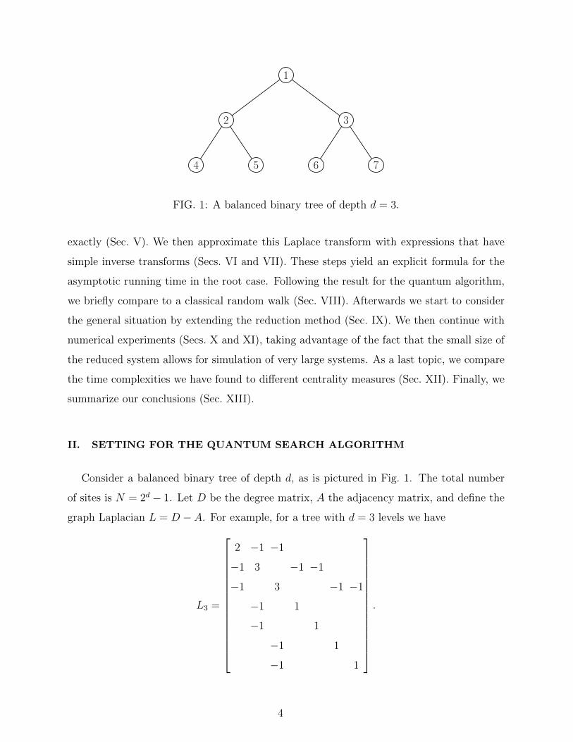
FIG. 1: A balanced binary tree of depth d = 3.

exactly (Sec. V). We then approximate this Laplace transform with expressions that have

simple inverse transforms (Secs. VI and VII). These steps yield an explicit formula for the

asymptotic running time in the root case. Following the result for the quantum algorithm,

we briefly compare to a classical random walk (Sec. VIII). Afterwards we start to consider

the general situation by extending the reduction method (Sec. IX). We then continue with

numerical experiments (Secs. X and XI), taking advantage of the fact that the small size of

the reduced system allows for simulation of very large systems. As a last topic, we compare

the time complexities we have found to different centrality measures (Sec. XII). Finally, we

summarize our conclusions (Sec. XIII).

II. SETTING FOR THE QUANTUM SEARCH ALGORITHM

Consider a balanced binary tree of depth d, as is pictured in Fig. 1. The total number

of sites is N = 2d − 1. Let D be the degree matrix, A the adjacency matrix, and define the

graph Laplacian L = D − A. For example, for a tree with d = 3 levels we have

L3 =

2 −1 −1

−1 3 −1 −1

−1 3 −1 −1

−1 1

−1 1

−1 1

−1 1

.

4

In the first part of this paper (up to Sec. VIII), we restrict our attention to the case where

the marked site |w〉 – the site that is being sought – is the root: |w〉 = |1〉. We study the

quantum search algorithm given by the Hamiltonian

H = γL− |w〉〈w|, (1)

which was proposed in Ref. [8]. The initial state is the uniform distribution,

|ψ(0)〉 = |s〉 =1√N

N∑k=1

|k〉.

Depending on the graph under consideration and on the location of the searched-for

site, there may exist values of the search parameter γ, for which evolution with respect to

H is very effective in shifting statistical weight towards |w〉 – for analyzing the algorithm

it is crucial to find these critical values γ∗. For example, Ref. [8] computes γ∗ for search

with (1) on a periodic lattice, and shows O(√N) time complexity in sufficiently large spatial

dimensions. For γ away from these critical points, however, the quantum algorithm fails to

provide speedup over the O(N) running time of classical search. Note that γ∗ might not be

constant as the system size increases.

III. REDUCTION IN GENERAL

We first review a technique for reducing the size of the system that was formally intro-

duced in Ref. [21]. Here, this approach is presented in an alternative way. In the following,

state vectors and operators in the reduced space will always be denoted with an overline.

Given H and an initial state ψ(0), the solution to an evolution problem is

ψ(t) = f(t,H)ψ(0),

where, for instance, f(t, z) = e−itz for evolution according to the Schrodinger equation. Now

suppose we have a linear reduction method V that transforms the system of size N to a

system of size n. The initial state in the reduced system is ψ(0) = V ψ(0). For the evolution

ψ(t) = f(t,H)ψ(0)

in the reduced system to reflect the dynamics of the original system, it is necessary that

ψ(t) = V ψ(t).

5

If f is analytic, we are lead to the condition

HkV ψ(0) = V Hkψ(0) for k ∈ N,

and hence to

V Hu = HV u for u ∈ U = spank≥0Hkψ(0). (2)

Let V + be the pseudoinverse of the n × N matrix V . For example, if V transforms a

graph of size 3 to a graph of size 2 by simply adding up the values of two of the sites, then

V and V + are

V =

1 0 0

0 1 1

, V + =

1 0

0 12

0 12

.The matrix V has full rank n, and therefore we have V V + = In. Now suppose that the

set on which V +V acts as the identity matrix coincides with the subspace U in (2). Then

we have

HV u = V Hu = V HV +V u,

and we obtain the operator

H = V HV + (3)

on the reduced space. H reproduces evolution starting from the initial state ψ(0) without

any loss of information (provided that the two conditions above are satisfied; for the spectra

of the two Hamiltonians we have σ(H) ⊆ σ(H), and the eigenvalues of H that are not in

σ(H) play no part in the dynamics since their eigenvectors do not overlap with ψ(0)).

IV. REDUCTION FOR THE TREE

We shall reduce the tree by combining all sites with the same distance to |w〉 = |1〉.

Hence the size of the reduced system is n = d, and we will use matrices of the form

V3 =

1

1√2

1√2

1√4

1√4

1√4

1√4

(for d = 4 append one row and eight columns and set the eight entries at the bottom right

equal to 1/√

8, etc.). For this reduction method we have V + = V >.

6

Define the states

|uj〉 =1√2j−1

2j−1∑k=2j−1

|k〉,

and note that

span1≤j≤n|uj〉 = spank≥0Hk|ψ(0)〉 = U.

Moreover, one can check that V +V |u〉 = |u〉 for |u〉 ∈ U . Therefore, by the theory from

the previous section, the reduction V is suitable for the quantum search problem under

consideration.

Letting the basis of the reduced space be

|j〉 = V |uj〉,

we obtain Hamiltonians of the form

H3 = γ

2− 1

γ−√

2 0

−√

2 3 −√

2

0 −√

2 1

(the matrix is tridiagonal for all n, the diagonal entries are γ · (2− 1

γ, 3, 3, . . . , 3, 1), and all

off-diagonal entries are −√

2 γ). The marked state of the reduced system is |w〉 = |1〉, and

the initial state is

|ψ(0)〉 = |s〉 = V |s〉 =1√N

n∑j=1

√2j−1 |j〉.

V. LAPLACE TRANSFORM OF THE STATE AT THE MARKED SITE

We are interested in the amplitude 〈ψ|w〉 = 〈ψ|1〉 = ψ1 of the wave vector at the searched-

for site. As a first step, we now compute its Laplace transform exactly. Note that ψ1 = ψ1.

Taking the Laplace transform of the evolution equation i∂tψ(t) = H ψ(t) gives

iαsψ(s)− iαψ(0) = αH ψ(s),

where α = γ−1. Writing out that system of equations, multiplying the k-th equation by

xk−1, and adding up all of them, we find

G(s;x) =

[1− 1+α√

2x]ψ1 +

[xn+1 −

√2xn]ψn +

iα√2N

n∑k=1

√2k−1xk

/(x2 − 3− iαs√

2x+ 1

),

(4)

7

for G(s;x) =∑n

k=1 ψk(s)xk−1. Denote the zeros of the denominator in (4) by x0 and x1 –

we have x0x1 = 1 and we let x0 be the zero that lies in the unit disk. Next we divide (4) by

x and integrate with respect to x over the unit circle. This leads to[x1 − 1+α√

2

]ψ1 +

[xn−10

(x0 −

√2)]ψn +

iα√2N

n∑k=1

(√2x0

)k−1= 0. (5)

We derive a second equation for ψ1 and ψn by multiplying (4) by x−n and again integrating

over the unit circle:[xn−10

(x0 − 1+α√

2

)]ψ1 +

[x1 −

√2]ψn +

iα√2N

n∑k=1

√2k−1xn−k0 = 0. (6)

Combining (5) and (6), we obtain an explicit formula for the Laplace transform of ψ1:

ψ1 =i√N

xn1 − xn0xn−11

[(is+ 1)x1 −

√2]− xn−10

[(is+ 1)x0 −

√2] . (7)

VI. APPROXIMATION FOR SMALL VALUES OF THE SEARCH PARAMETER

We will now find an approximation of ψ1 in the range γ ∈ [0, 1− ε], and we will see that

the algorithm fails for those values of the search parameter. Hence the critical value γ∗ must

be 1 or larger. That is noteworthy, since in most known examples γ∗ tends to small positive

constants or to zero as N → ∞ – the general trend is γ∗ ∼ 1δ, where δ is the degree of the

searched-for site [2, 6, 8, 19, 21, 23, 24].

Recall the definition of x0 and x1 after (4). Since |x0| < 1, we have xn0 → 0 and (7) yields

ψ1 ≈i√N

x1

(is+ 1)x1 −√

2(8)

for large n. This expression has poles s = 0 and s = iα−1α+1

, and computing the corresponding

residues gives

ψ1 ≈1√N

[1

1− α· 1 +

α2 + 2α− 1

α2 − 1· ei

α−1α+1

t

], (9)

where α = γ−1.

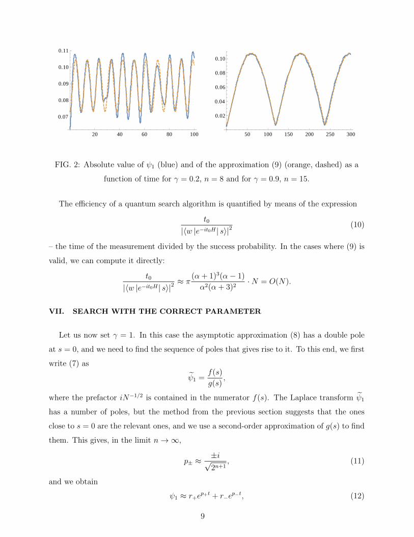
Numerical experiments show that (9) is adequate for γ ∈ [0, 1 − ε], c.f. Fig. 2. Note

that (9) gives the exact solution for γ = 0. However, the low success probabilities in Fig. 2

(as well as the fact that the frequency does not explicitly depend on n) suggest that the

oscillations in this range of γ are trivial and not useful for finding the marked site.

8

20 40 60 80 100

0.07

0.08

0.09

0.10

0.11

50 100 150 200 250 300

0.02

0.04

0.06

0.08

0.10

FIG. 2: Absolute value of ψ1 (blue) and of the approximation (9) (orange, dashed) as a

function of time for γ = 0.2, n = 8 and for γ = 0.9, n = 15.

The efficiency of a quantum search algorithm is quantified by means of the expression

t0

|〈w |e−it0H | s〉|2(10)

– the time of the measurement divided by the success probability. In the cases where (9) is

valid, we can compute it directly:

t0

|〈w |e−it0H | s〉|2≈ π

(α + 1)3(α− 1)

α2(α + 3)2·N = O(N).

VII. SEARCH WITH THE CORRECT PARAMETER

Let us now set γ = 1. In this case the asymptotic approximation (8) has a double pole

at s = 0, and we need to find the sequence of poles that gives rise to it. To this end, we first

write (7) as

ψ1 =f(s)

g(s),

where the prefactor iN−1/2 is contained in the numerator f(s). The Laplace transform ψ1

has a number of poles, but the method from the previous section suggests that the ones

close to s = 0 are the relevant ones, and we use a second-order approximation of g(s) to find

them. This gives, in the limit n→∞,

p± ≈±i√2n+1

, (11)

and we obtain

ψ1 ≈ r+ep+t + r−e

p−t, (12)

9

100 200 300 400 500 600

0.1

0.2

0.3

0.4

0.5

0.6

0.7

200 400 600 800 1000 1200

0.1

0.2

0.3

0.4

0.5

0.6

0.7

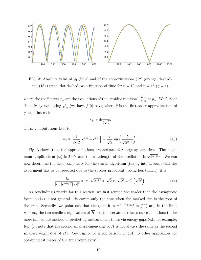
FIG. 3: Absolute value of ψ1 (blue) and of the approximations (12) (orange, dashed)

and (13) (green, dot-dashed) as a function of time for n = 10 and n = 15 (γ = 1).

where the coefficients r± are the evaluations of the “residue function” f(s)g′(s)

at p±. We further

simplify by evaluating ig(s)

(we have f(0) ≈ i), where g is the first-order approximation of

g′ at 0, instead:

r± ≈ ±1

2√

2.

These computations lead to

ψ1 ≈1

2√

2

[ep+t − ep−t

]=

i√2

sin

(t√

2n+1

). (13)

Fig. 3 shows that the approximations are accurate for large system sizes. The maxi-

mum amplitude at |w〉 is 2−1/2 and the wavelength of the oscillation is√

2n+3 π. We can

now determine the time complexity for the search algorithm (taking into account that the

experiment has to be repeated due to the success probability being less than 1), it is

t0

|〈w |e−it0H | s〉|2≈ π ·

√2n+1 ≈

√2 π ·√N = Θ

(√N). (14)

As concluding remarks for this section, we first remind the reader that the asymptotic

formula (14) is not general – it covers only the case when the marked site is the root of

the tree. Secondly, we point out that the quantities ±2−(n+1)/2 in (11) are, in the limit

n→∞, the two smallest eigenvalues of H – this observation relates our calculations to the

more immediate method of predicting measurement times via energy gaps (c.f., for example,

Ref. [8]; note that the second smallest eigenvalue of H is not always the same as the second

smallest eigenvalue of H). See Fig. 5 for a comparison of (14) to other approaches for

obtaining estimates of the time complexity.

10

VIII. SEARCH WITH A CLASSICAL RANDOM WALK

We briefly compare to the performance of a classical random walker. Suppose the walker

is randomly placed in the tree – how long does it take to locate the root (i.e. the one site

that has degree 2)?

Let tk be the average time a random walker that starts from a site on level k needs to

find the root. Then we have

t1 = 0,

tk = 13tk−1 + 2

3tk+1 + 1,

tn = tn−1 + 1.

(15)

Define the weighted times tk and the average search time T :

tk =2k−1

Ntk, T =

n∑k=1

tk.

Then (15) leads to

N ·

1 · 2−1 −23· 2−2

−13· 2−1 1 · 2−2 −2

3· 2−3

−13· 2−2 1 · 2−3

. . .

1 · 2−(n−2) −23· 2−(n−1)

−1 · 2−(n−2) 1 · 2−(n−1)

·

t2

t3

t4...

tn−1

tn

=

1

1

1...

1

1

.

We next renormalize the diagonal by multiplying all equations by appropriate powers of 2,

and then we add all of them. This gives

N − 1

N=[1− 1

3− 2

3

]T + 1

3t2 − 4

3tn−1 + 2

3tn,

and consequently

t2 = N − 2.

Hence, since the walker needs linear time even when starting from a neighbor of the

searched-for site, we have Ω(N) (i.e. at least ∼ N) average time complexity for this classical

approach, and we see that the quantum algorithm provides a significant speedup. As a side

note we point out that in Ref. [15] it was shown that the average hitting times for random

walks on arbitrary trees are always integers.

11

IX. REDUCTION IN THE GENERAL CASE

We now generalize our reduction method and allow |w〉 to be anywhere in the tree. We

denote the level on which the marked site is by l (and n is the total number of levels,

as before). We will see below that we can reduce the full system to one of size less than

n2 = (logN)2 in a way similar to what has been done in Sec. IV. Eq. (3) for the Hamiltonian

in the reduced system, H = V HV +, is still valid and useful, but the necessary conditions

are not constructive – they do not show how to find the matrix V . We use the following

intuitive argument (as has been done, for instance, in Ref. [23]): We can group together sites

that are indistinguishable in the sense that (a) their positions in the graph are qualitatively

the same, and (b) their positions relative to |w〉 are the same. For example, for grouping

sites together it is certainly necessary that they (a) have the same degree, and (b) have the

same distance from |w〉.

An illustration of this reduction is given by Fig. 4. We can see how the full tree is

transformed into a comb-structure. We consider |w〉, all its ancestors, and the combination

of its two children the back-bone of that comb. Then we can transform the system to

a line-graph by absorbing the side-chains into the back-bone. However, this leads to an

inhomogeneous Hamiltonian with non-constant coefficients. The formula for absorption

into ancestors of the searched-for site is[1 + xm0

(x0 −

√2)xm0 − xm1x0 − x1

]φ1 =

1√2

[x0 + xm0

(x0 −

√2)xm−10 − xm−11

x0 − x1

]φ0

− 1√N

[xm0(x0 −

√2)

s

(√

2m−1− xm0 − xm1

x0 − x1+

1√2

xm−10 − xm−11

x0 − x1

)+iαx0√

2

1−(√

2x0)m

1−√

2x0

]

in Laplace space, where φ0 is the back-bone site into which we want to absorb, φ1 is the

first element of the side-chain we want to eliminate, and m is its size. For the absorption

below |w〉, we have the same expression with the φ0 term and the constant term changing

by factors of√

2 and 2, respectively.

The system in Fig. (4c) might be useful for analytical considerations, but we will not

work with it in the remainder of our analysis. Instead we focus on numerical simulations

of (4b), which is of size at most ≈ n2

2. For H we could generate the N × N matrix H and

the reduction matrix V and then apply (3). After that we can use the much smaller matrix

H for operations such as finding eigenvalues and for repeated evaluations of the propagator.

12

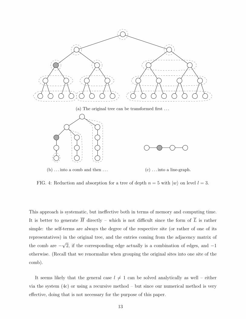
(a) The original tree can be transformed first . . .

(b) . . . into a comb and then . . . (c) . . . into a line-graph.

FIG. 4: Reduction and absorption for a tree of depth n = 5 with |w〉 on level l = 3.

This approach is systematic, but ineffective both in terms of memory and computing time.

It is better to generate H directly – which is not difficult since the form of L is rather

simple: the self-terms are always the degree of the respective site (or rather of one of its

representatives) in the original tree, and the entries coming from the adjacency matrix of

the comb are −√

2, if the corresponding edge actually is a combination of edges, and −1

otherwise. (Recall that we renormalize when grouping the original sites into one site of the

comb).

It seems likely that the general case l 6= 1 can be solved analytically as well – either

via the system (4c) or using a recursive method – but since our numerical method is very

effective, doing that is not necessary for the purpose of this paper.

13

0 0.5 1 1.5 2 2.5 3 3.5

x 104

0

100

200

300

400

500

600

700

800

900

N

t 0/p

0

asymptotic formula

via gaps

read−off data

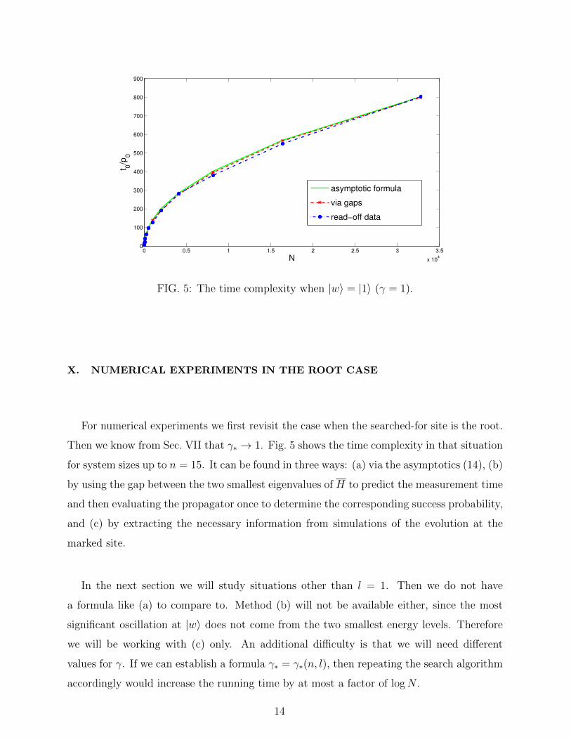
FIG. 5: The time complexity when |w〉 = |1〉 (γ = 1).

X. NUMERICAL EXPERIMENTS IN THE ROOT CASE

For numerical experiments we first revisit the case when the searched-for site is the root.

Then we know from Sec. VII that γ∗ → 1. Fig. 5 shows the time complexity in that situation

for system sizes up to n = 15. It can be found in three ways: (a) via the asymptotics (14), (b)

by using the gap between the two smallest eigenvalues of H to predict the measurement time

and then evaluating the propagator once to determine the corresponding success probability,

and (c) by extracting the necessary information from simulations of the evolution at the

marked site.

In the next section we will study situations other than l = 1. Then we do not have

a formula like (a) to compare to. Method (b) will not be available either, since the most

significant oscillation at |w〉 does not come from the two smallest energy levels. Therefore

we will be working with (c) only. An additional difficulty is that we will need different

values for γ. If we can establish a formula γ∗ = γ∗(n, l), then repeating the search algorithm

accordingly would increase the running time by at most a factor of logN .

14

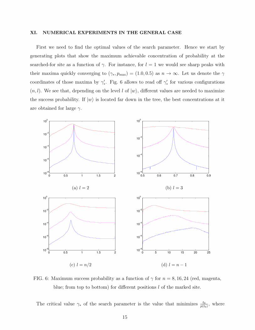
XI. NUMERICAL EXPERIMENTS IN THE GENERAL CASE

First we need to find the optimal values of the search parameter. Hence we start by

generating plots that show the maximum achievable concentration of probability at the

searched-for site as a function of γ. For instance, for l = 1 we would see sharp peaks with

their maxima quickly converging to (γ∗, pmax) = (1.0, 0.5) as n → ∞. Let us denote the γ

coordinates of those maxima by γ′∗. Fig. 6 allows to read off γ′∗ for various configurations

(n, l). We see that, depending on the level l of |w〉, different values are needed to maximize

the success probability. If |w〉 is located far down in the tree, the best concentrations at it

are obtained for large γ.

0 0.5 1 1.5 210

−8

10−6

10−4

10−2

100

(a) l = 2

0.5 0.6 0.7 0.8 0.910

−6

10−4

10−2

100

(b) l = 3

0 0.5 1 1.5 210

−8

10−6

10−4

10−2

100

(c) l = n/2

0 5 10 15 20 2510

−8

10−6

10−4

10−2

100

(d) l = n− 1

FIG. 6: Maximum success probability as a function of γ for n = 8, 16, 24 (red, magenta,

blue; from top to bottom) for different positions l of the marked site.

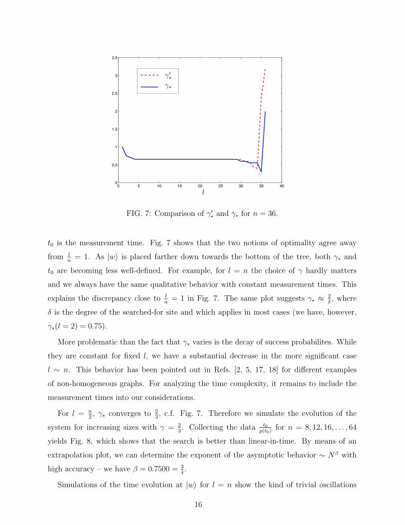
The critical value γ∗ of the search parameter is the value that minimizes t0p(t0)

, where

15

0 5 10 15 20 25 30 35 400

0.5

1

1.5

2

2.5

3

3.5

γ′∗γ∗

l

FIG. 7: Comparison of γ′∗ and γ∗ for n = 36.

t0 is the measurement time. Fig. 7 shows that the two notions of optimality agree away

from ln

= 1. As |w〉 is placed farther down towards the bottom of the tree, both γ∗ and

t0 are becoming less well-defined. For example, for l = n the choice of γ hardly matters

and we always have the same qualitative behavior with constant measurement times. This

explains the discrepancy close to ln

= 1 in Fig. 7. The same plot suggests γ∗ ≈ 2δ, where

δ is the degree of the searched-for site and which applies in most cases (we have, however,

γ∗(l = 2) = 0.75).

More problematic than the fact that γ∗ varies is the decay of success probabilites. While

they are constant for fixed l, we have a substantial decrease in the more significant case

l ∼ n. This behavior has been pointed out in Refs. [2, 5, 17, 18] for different examples

of non-homogeneous graphs. For analyzing the time complexity, it remains to include the

measurement times into our considerations.

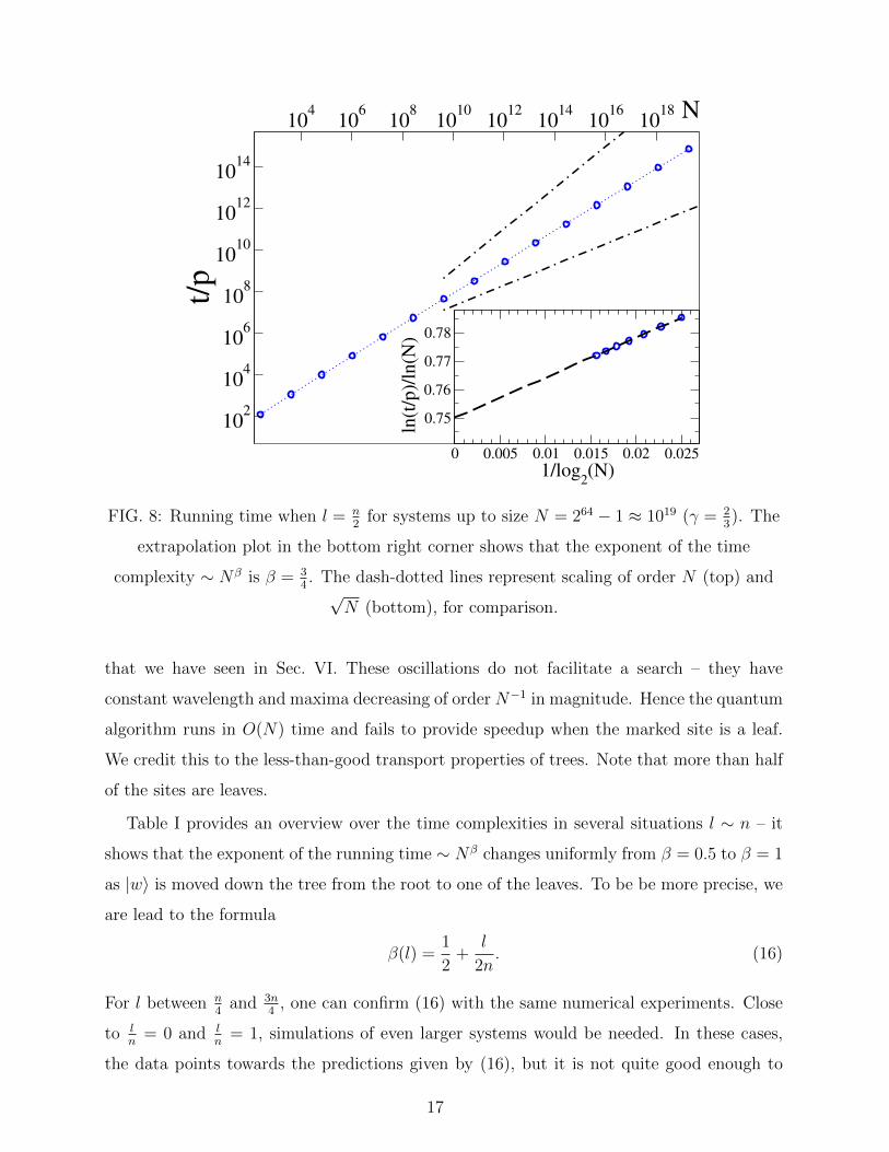
For l = n2, γ∗ converges to 2

3, c.f. Fig. 7. Therefore we simulate the evolution of the

system for increasing sizes with γ = 23. Collecting the data t0

p(t0)for n = 8, 12, 16, . . . , 64

yields Fig. 8, which shows that the search is better than linear-in-time. By means of an

extrapolation plot, we can determine the exponent of the asymptotic behavior ∼ Nβ with

high accuracy – we have β = 0.7500 = 34.

Simulations of the time evolution at |w〉 for l = n show the kind of trivial oscillations

16

0 0.005 0.01 0.015 0.02 0.025

1/log2(N)

0.75

0.76

0.77

0.78

ln(t/p)/ln(N

)

104

106

108

1010

1012

1014

1016

1018 N

102

104

106

108

1010

1012

1014

t/p

FIG. 8: Running time when l = n2

for systems up to size N = 264 − 1 ≈ 1019 (γ = 23). The

extrapolation plot in the bottom right corner shows that the exponent of the time

complexity ∼ Nβ is β = 34. The dash-dotted lines represent scaling of order N (top) and√N (bottom), for comparison.

that we have seen in Sec. VI. These oscillations do not facilitate a search – they have

constant wavelength and maxima decreasing of order N−1 in magnitude. Hence the quantum

algorithm runs in O(N) time and fails to provide speedup when the marked site is a leaf.

We credit this to the less-than-good transport properties of trees. Note that more than half

of the sites are leaves.

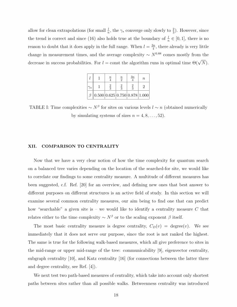
Table I provides an overview over the time complexities in several situations l ∼ n – it

shows that the exponent of the running time ∼ Nβ changes uniformly from β = 0.5 to β = 1

as |w〉 is moved down the tree from the root to one of the leaves. To be be more precise, we

are lead to the formula

β(l) =1

2+

l

2n. (16)

For l between n4

and 3n4

, one can confirm (16) with the same numerical experiments. Close

to ln

= 0 and ln

= 1, simulations of even larger systems would be needed. In these cases,

the data points towards the predictions given by (16), but it is not quite good enough to

17

allow for clean extrapolations (for small ln, the γ∗ converge only slowly to 2

3). However, since

the trend is correct and since (16) also holds true at the boundary of ln∈ [0, 1], there is no

reason to doubt that it does apply in the full range. When l = 3n4

, there already is very little

change in measurement times, and the average complexity ∼ N0.88 comes mostly from the

decrease in success probabilities. For l = const the algorithm runs in optimal time Θ(√N).

l 1 n4

n2

3n4 n

γ∗ 1 23

23

23 2

β 0.500 0.625 0.750 0.878 1.000

TABLE I: Time complexities ∼ Nβ for sites on various levels l ∼ n (obtained numerically

by simulating systems of sizes n = 4, 8, . . . , 52).

XII. COMPARISON TO CENTRALITY

Now that we have a very clear notion of how the time complexity for quantum search

on a balanced tree varies depending on the location of the searched-for site, we would like

to correlate our findings to some centrality measure. A multitude of different measures has

been suggested, c.f. Ref. [20] for an overview, and defining new ones that best answer to

different purposes on different structures is an active field of study. In this section we will

examine several common centrality measures, our aim being to find one that can predict

how “searchable” a given site is – we would like to identify a centrality measure C that

relates either to the time complexity ∼ Nβ or to the scaling exponent β itself.

The most basic centrality measure is degree centrality, CD(v) = degree(v). We see

immediately that it does not serve our purpose, since the root is not ranked the highest.

The same is true for the following walk-based measures, which all give preference to sites in

the mid-range or upper mid-range of the tree: communicability [9], eigenvector centrality,

subgraph centrality [10], and Katz centrality [16] (for connections between the latter three

and degree centrality, see Ref. [4]).

We next test two path-based measures of centrality, which take into account only shortest

paths between sites rather than all possible walks. Betweenness centrality was introduced

18

in Ref. [12] and is defined as follows:

CB(v) =∑i 6=v

∑j 6=v

δij(v),

where δij(v) is the number of shortest paths from i to j that pass through v divided by the

total number of shortest paths from i to j. The formula for closeness centrality [13] is

CC(v) =(∑

j

d(j, v))−1

,

where d(j, v) is distance between j and v. We produce normalized centralities CB and CC

by dividing by the largest values of CB and CC a site in a graph of size N can possibly have.

These factors come, in both cases, from the center site of the star graph.

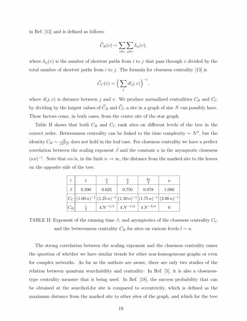
Table II shows that both CB and CC rank sites on different levels of the tree in the

correct order. Betweenness centrality can be linked to the time complexity ∼ Nβ, but the

identity CB ∼ N(Nβ)2

does not hold in the leaf case. For closeness centrality we have a perfect

correlation between the scaling exponent β and the constant κ in the asymptotic closeness

(κn)−1. Note that κn is, in the limit n→∞, the distance from the marked site to the leaves

on the opposite side of the tree.

l 1 n4

n2

3n4 n

β 0.500 0.625 0.750 0.878 1.000

CC (1.00n)−1 (1.25n)−1 (1.50n)−1 (1.75n)−1 (2.00n)−1

CB12 4N−1/4 4N−1/2 4N−3/4 0

TABLE II: Exponent of the running time β, and asymptotics of the closeness centrality CC

and the betweenness centrality CB for sites on various levels l ∼ n.

The strong correlation between the scaling exponent and the closeness centrality raises

the question of whether we have similar trends for other non-homogeneous graphs or even

for complex networks. As far as the authors are aware, there are only two studies of the

relation between quantum searchability and centrality: In Ref. [5], it is also a closeness-

type centrality measure that is being used. In Ref. [18], the success probability that can

be obtained at the searched-for site is compared to eccentricity, which is defined as the

maximum distance from the marked site to other sites of the graph, and which for the tree

19

under consideration is asymptotically equal to C−1C (c.f. remark at the end of the previous

paragraph).

XIII. CONCLUSIONS

In this paper we presented an analysis of a continuous-time quantum search algorithm

on balanced binary trees. We saw that the running time depends on the location of the

marked site. If it is a leaf that is being sought, there is no improvement of the linear-in-

size running time of classical algorithms. However, the root can be found with quadratic

speedup, in Θ(√N) time. In between these two cases, the exponent of the time complexity

∼ Nβ changes linearly from β = 0.5 to β = 1. Our work relied heavily on a dimensionality

reduction method, which, besides allowing to perform numerical experiments with very large

systems, was also crucial for symbolic computations in a special case.

We would like to point out that our results do not imply that there is no effective

continuous-time quantum algorithm for search on a balanced tree – with (1) we have only

studied the most commonly used Hamiltonian for that purpose. For example, by changing

the weights of some of the edges of a certain graph, Ref. [23] improved the running time

from Θ(N3/4) to nearly Θ(N1/2).

We have also examined the relation of how effectively a site can be searched with its

centrality, and we have found a strong correlation between the scaling exponent β and

closeness centrality. Since balanced binary trees are highly non-generic structures, more

evidence is needed before one can formulate a general hypothesis. Given the apparent

limited amount of studies on this topic, Refs. [5, 18], it would be interesting to see more

examples of quantum walks on non-homogeneous graphs, and to compare the differences in

time complexities to closeness or other centrality measures.

As a concluding remark, we would like to compare our work to Ref. [7]. In that paper,

the authors study a pair of balanced trees that are glued together along the leaves, and they

show propagation from one root to the other in O(log(N)) time. In our framework, this

corresponds to extending the reduced matrix in Sec. IV by an identical flipped copy, so that

the quantum walk on a large structure is instead performed on a line of length ∼ log(N).

Ref. [7] does not contradict the poor efficiency we have found in the case when the searched-

for site is a leaf – instead it shows that there is a significant difference between transporting

20

to one particular leaf and transporting to the collection of all leaves.

ACKNOWLEDGEMENTS

PP and LT were supported by CNPq CSF / BJT grants 400216/2014-0 and 301181/2014-

4. SB acknowledges financial support from the U. S. National Science Foundation through

grant DMR-1207431 and from CNPq through the “Ciencia sem Fronteiras” program, and

thanks LNCC for its hospitality. PP and LT would further like to thank Renato Portugal

and Isabel Chen-Philipp for useful discussions.

[1] Aaronson, S. and Ambainis, A. (2003). Quantum search of spatial regions. In Foundations of

Computer Science, 2003. Proceedings. 44th Annual IEEE Symposium on, pages 200–209.

[2] Agliari, E., Blumen, A., and Mulken, O. (2010). Quantum-walk approach to searching on

fractal structures. Phys. Rev. A, 82:012305.

[3] Bennett, C. H., Bernstein, E., Brassard, G., and Vazirani, U. (1997). Strengths and weaknesses

of quantum computing. SIAM J. Comput., 26(5):1510–1523.

[4] Benzi, M. and Klymko, C. (2015). On the limiting behavior of parameter-dependent network

centrality measures. SIAM Journal on Matrix Analysis and Applications, 36(2):686–706.

[5] Berry, S. and Wang, J. (2010). Quantum-walk-based search and centrality. Physical Review

A, 82:Article number 042333, 12pp.

[6] Chakraborty, S., Novo, L., Ambainis, A., and Omar, Y. (2015). Spatial search by quantum

walk is optimal for almost all graphs. ArXiv e-prints.

[7] Childs, A. M., Farhi, E., and Gutmann, S. (2002). An example of the difference between

quantum and classical random walks. Quantum Information Processing, 1(1):35–43.

[8] Childs, A. M. and Goldstone, J. (2004). Spatial search by quantum walk. Phys. Rev. A,

70:022314.

[9] Estrada, E. and Hatano, N. (2008). Communicability in complex networks. Phys. Rev. E,

77:036111.

[10] Estrada, E. and Rodrıguez-Velazquez, J. A. (2005). Subgraph centrality in complex networks.

Phys. Rev. E, 71:056103.

21

[11] Farhi, E. and Gutmann, S. (1998). Analog analogue of a digital quantum computation. Phys.

Rev. A, 57:2403–2406.

[12] Freeman, L. C. (1977). A set of measures of centrality based on betweenness. Sociometry,

40(1):35–41.

[13] Freeman, L. C. (1979). Centrality in social networks conceptual clarification. Social networks,

1(3):215–239.

[14] Grover, L. K. (1996). A fast quantum mechanical algorithm for database search. In Proceedings

of the Twenty-eighth Annual ACM Symposium on Theory of Computing, STOC ’96, pages

212–219, New York, NY, USA. ACM.

[15] Haiyan, C. and Fuji, Z. (2004). The expected hitting times for graphs with cutpoints. Statistics

& Probability Letters, 66(1):9 – 17.

[16] Katz, L. (1953). A new status index derived from sociometric analysis. Psychometrika,

18(1):39–43.

[17] Lovett, N., Everitt, M., Trevers, M., Mosby, D., Stockton, D., and Kendon, V. (2012). Spatial

search using the discrete time quantum walk. Natural Computing, 11(1):23–35.

[18] Mahasinghe, A., Wang, J. B., and Wijerathna, J. K. (2014). Quantum walk-based search and

symmetries in graphs. Journal of Physics A: Mathematical and Theoretical, 47(50):505301.

[19] Meyer, D. A. and Wong, T. G. (2015). Connectivity is a poor indicator of fast quantum

search. Phys. Rev. Lett., 114:110503.

[20] Newman, M. (2010). Networks: An Introduction. Oxford University Press, Inc., New York,

NY, USA.

[21] Novo, L., Chakraborty, S., Mohseni, M., Neven, H., and Omar, Y. (2015). Systematic dimen-

sionality reduction for quantum walks: Optimal spatial search and transport on non-regular

graphs. Scientific Reports, 5:13304 EP –.

[22] Paparo, G. D., Muller, M., Comellas, F., and Martin-Delgado, M. A. (2013). Quantum google

in a complex network. Scientific Reports, 3:2773 EP –.

[23] Wong, T. G. (2015a). Faster quantum walk search on a weighted graph. Phys. Rev. A,

92:032320.

[24] Wong, T. G. (2015b). Spatial Search by Continuous-Time Quantum Walk with Multiple

Marked Vertices. ArXiv e-prints.

22