Continuous time and Discrete time Signals and Systems · PDF fileContinuous time and Discrete...
17
Signals and Systems Lecture: 1 Dr. Ayman Elshenawy Elsefy Page | 1 Continuous time and Discrete time Signals and Systems 1. Systems in Engineering A system is usually understood to be an engineering device in the field, and a mathematical representation of this system is usually called a system model . It can be defined as the mathematical relationship between an input signal and an output signal. The word system refers to many different things in engineering, It may be refers to: Tangible objects: such as software systems, electronic systems, computer systems, or mechanical systems. Theoretical objects: such as a system of linear equations or a mathematical input- output model. 2. Signals Signals are functions of time that represent the evolution of variables and describe a wide variety of physical phenomena. Signals carry information about these physical phenomena in a pattern of variation of some forms. Signals are represented mathematically as functions of one (one dimensional signal) or more independent variables ( multi-dimensional signal). It can be classified from the independent variable nature into two types: Continuous Time (CT): If the independent variable is continuous this refers to Continuous Time signal x(t). These signals are defined for continuum of values of the independent variable. Discrete Time (DT): signals x[n] are defined only at discrete times and the independent variable takes only a discrete set of values. They are defined only for integer values of the independent variable ( time steps). Consider the simple circuit shown in Fig.1 the pattern of variation over time in the source and capacitor voltage V and V . Similarly, in Fig. 2, the variation of the applied force f over time resulting in automobile velocity V.
Transcript of Continuous time and Discrete time Signals and Systems · PDF fileContinuous time and Discrete...

Signals and Systems Lecture: 1
Dr. Ayman Elshenawy Elsefy Page | 1
Continuous time and Discrete time Signals and Systems
1. Systems in Engineering
A system is usually understood to be an engineering device in the field, and a mathematical
representation of this system is usually called a system model. It can be defined as the
mathematical relationship between an input signal and an output signal. The word system
refers to many different things in engineering, It may be refers to:
Tangible objects: such as software systems, electronic systems, computer systems,
or mechanical systems.
Theoretical objects: such as a system of linear equations or a mathematical input-
output model.
2. Signals
Signals are functions of time that represent the evolution of variables and describe a wide
variety of physical phenomena. Signals carry information about these physical phenomena in a
pattern of variation of some forms. Signals are represented mathematically as functions of one
(one dimensional signal) or more independent variables (multi-dimensional signal). It can be
classified from the independent variable nature into two types:
Continuous Time (CT): If the independent variable is continuous this refers to
Continuous Time signal x(t). These signals are defined for continuum of values of
the independent variable.
Discrete Time (DT): signals x[n] are defined only at discrete times and the
independent variable takes only a discrete set of values. They are defined only for
integer values of the independent variable (time steps).
Consider the simple circuit shown in Fig.1 the pattern of variation over time in the source
and capacitor voltage V and V . Similarly, in Fig. 2, the variation of the applied force f over
time resulting in automobile velocity V.

Signals and Systems Lecture: 1
Dr. Ayman Elshenawy Elsefy Page | 2
Fig. 1: A simple RC circuit Fig.2 : An automobile responding to a force f
Fig. 3: Recording of human speech Fig. 4: A monochromatic picture
Fig. 5: annual vertical wind profile Fig. 6: A discrete time signal
Fig. 7 : A Continous Time signal and discrete Time signal
Fig.3 is an illustration of a recording of human speech signal using microphone to sense
acoustic pressure. Speech
The monochromatic picture shown in Fig. 4, it represents the pattern of variation in
brightness versus the (x, y) position of the image. Brightness

Signals and Systems Lecture: 1
Dr. Ayman Elshenawy Elsefy Page | 3
In geophysics, signals representing variations with depth of physical quantities such as
density, porosity, and electrical resistivity are used to study the structure of the earth.
In metrological investigations, the knowledge of air pressure, temperature and wind speed
with latitude are extremely important. Fig. 5 describes an annual average of vertical wind
profile as function of height. Used in weather patterns and aircraft landing and final
approach. Fig. 7 represents a graphical illustration of CT and DT signal.
How to obtain discrete signal from continuous signal?
Discrete signals often arise from signals with continuous domains by sampling. Continuous
domains have an infinite number of elements. Even the domain [0,1] Time representing a
finite time interval has an infinite number of elements. The signal assigns a value in its range
to each of these infinitely many elements. Such a signal cannot be stored in a finite digital
memory device such as a computer or CD-ROM. If we wish to store, say, Voice, we must
approximate it by a signal with a finite domain. A common way to approximate a function
with a continuous domain like Voice and Image by a function with a finite domain is by
uniformly sampling its continuous domain.
Fig. 8: The exponential functions and Sampled Exp, with sampling interval of 0.2.
If we sample a 10-second long domain of Voice [0,10], 10,000 times per second (i.e. at a
frequency of 10 kHz) we get the signal Sampled Voice ={0,0.0001,0.0002, … , 9.9998,
9.9999,10}. In the example, the sampling interval or sampling period is 0.0001 sec,
corresponding to a sampling frequency or sampling rate of 10,000 Hz. Since the continuous
domain is 10 seconds long, the domain of Sampled Voice has 100,000 points. A sampling
frequency of 5,000 Hz would give the Sampled Voice ={0,0.0002,0.0004, … , 9.9998,10},

Signals and Systems Lecture: 1
Dr. Ayman Elshenawy Elsefy Page | 4
which has half as many points. The sampled domain is finite, and its elements are discrete
values of time.
Fig. 8 shows an exponential function and it’s sampled signal with sampling interval= 0.2
Continuous-time and discrete-time functions map their domain (time interval) into their co-
domain (range or set of values). This is expressed in mathematical notation as : . As
shown in Fig. 9.
Fig. 9: Domain, co-domain, and range of a real function of continuous time.
3. Transformation of the Independent Variable
Consider the continuous-time signal x(t) defined by its graph shown in Fig. 10 and the
discrete-time signal x[n] defined by its graph in Fig. 11. As an aside, these two signals are said
to be of finite support, as they are nonzero only over a finite time interval, namely on
[ 2,2] for x(t) and { 3, … ,3} when for x[n]. We will use these two signals to illustrate
some useful transformations of the time variable, such as time scaling and time reversal.
Time Scaling
Time scaling refers to the multiplication of the time variable by a real positive constant .
In the continuous-time case, we can write ( ) = ( )
In case 0 < < 1: The signal x(t) is slowed down or expanded (stretched) in time. Think
of a tape recording played back at a slower speed than the nominal speed.
In case > 1: The signal x(t) is sped up or compressed in time. Think of a tape recording
played back at twice the nominal speed
Try to guess the behavior in case < 0 …………………………………………………..

Signals and Systems Lecture: 1
Dr. Ayman Elshenawy Elsefy Page | 5
In the discrete time case, we can write [ ] = [ ]
In case > 1: where is an integer, makes sense, as x[n] is undefined for fractional values of
n. In this case, called decimation or down-sampling, we not only get a time compression of the
signal, but the signal can also lose part of its information; that is, some of its values may
disappear in the resulting signal y[n].
A continuous Time Signal x(t) A Discrete Time Signal x[n]
Time scaling ( ) = (0.5 ), = 0.5 Time scaling [n] = [2n], = 2
Time scaling y(t) = x(2t), = 2
Fig. 10: Transformation of the independent variable (Time scaling ) on CT and DT signal
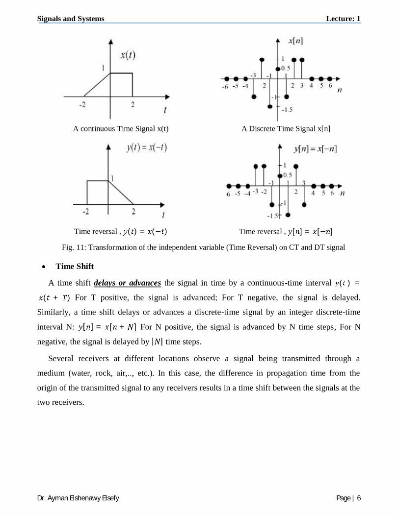
Time Reversal
A time reversal is achieved by multiplying the time variable by –1. If ( ) represents an
audio tap recording, then ( ) is the same tap recording played back word.
Signals and Systems Lecture: 1
Dr. Ayman Elshenawy Elsefy Page | 6
A continuous Time Signal x(t) A Discrete Time Signal x[n]
Time reversal , ( ) = ( ) Time reversal , [ ] = [ ]
Fig. 11: Transformation of the independent variable (Time Reversal) on CT and DT signal
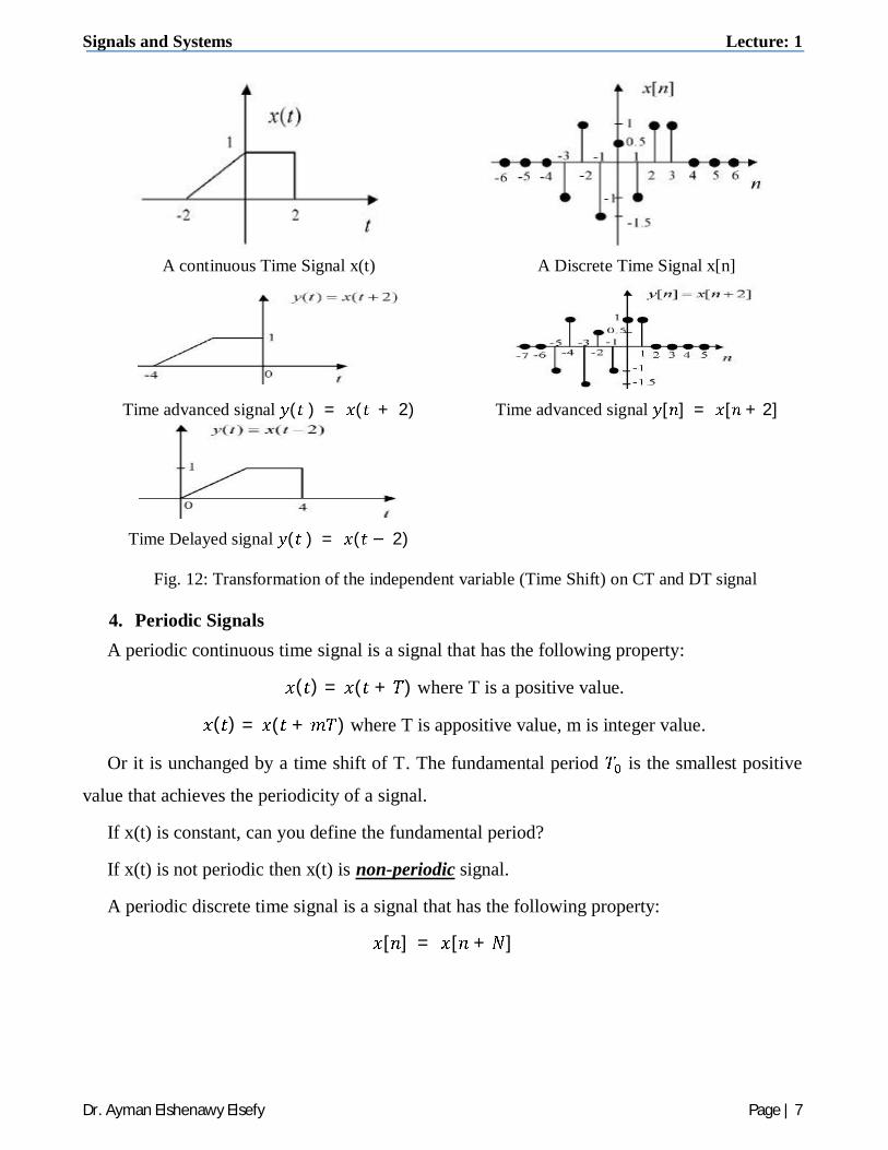
Time Shift
A time shift delays or advances the signal in time by a continuous-time interval ( ) =
( + ) For T positive, the signal is advanced; For T negative, the signal is delayed.
Similarly, a time shift delays or advances a discrete-time signal by an integer discrete-time
interval N: [ ] = [ + ] For N positive, the signal is advanced by N time steps, For N
negative, the signal is delayed by | | time steps.
Several receivers at different locations observe a signal being transmitted through a
medium (water, rock, air,.., etc.). In this case, the difference in propagation time from the
origin of the transmitted signal to any receivers results in a time shift between the signals at the
two receivers.
Signals and Systems Lecture: 1
Dr. Ayman Elshenawy Elsefy Page | 7
A continuous Time Signal x(t) A Discrete Time Signal x[n]
Time advanced signal ( ) = ( + 2) Time advanced signal [ ] = [ + 2]
Time Delayed signal ( ) = ( 2)
Fig. 12: Transformation of the independent variable (Time Shift) on CT and DT signal
4. Periodic Signals A periodic continuous time signal is a signal that has the following property:
( ) = ( + ) where T is a positive value.
( ) = ( + ) where T is appositive value, m is integer value.
Or it is unchanged by a time shift of T. The fundamental period is the smallest positive
value that achieves the periodicity of a signal.
If x(t) is constant, can you define the fundamental period?
If x(t) is not periodic then x(t) is non-periodic signal.
A periodic discrete time signal is a signal that has the following property:
[ ] = [ + ]
Signals and Systems Lecture: 1
Dr. Ayman Elshenawy Elsefy Page | 8
Fig. 13: A continuous time and Discrete time Periodic signal
The fundamental period is the smallest positive value of N that achieves the periodicity
of a signal. Examples of periodic continuous and discrete time signals are shown in Fig. 11.
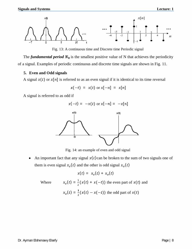
5. Even and Odd signals A signal ( ) or [ ] is referred to as an even signal if it is identical to its time reversal
( ) = ( ) or [ ] = [ ]
A signal is referred to as odd if
( ) = ( ) or [ ] = [ ]
Fig. 14: an example of even and odd signal
An important fact that any signal ( )can be broken to the sum of two signals one of
them is even signal ( ) and the other is odd signal ( )
( ) = ( ) + ( )
Where ( ) = ( ( ) + ( )) the even part of ( ) and
( ) = ( ( ) ( )) the odd part of ( )

Signals and Systems Lecture: 1
Dr. Ayman Elshenawy Elsefy Page | 9
Fig. 15: an example of the even and odd decomposition of discrete time signal
Signals and Systems Solved Exercise on Lecture 1
Dr. Ayman Elshenawy Elsefy Page | 1
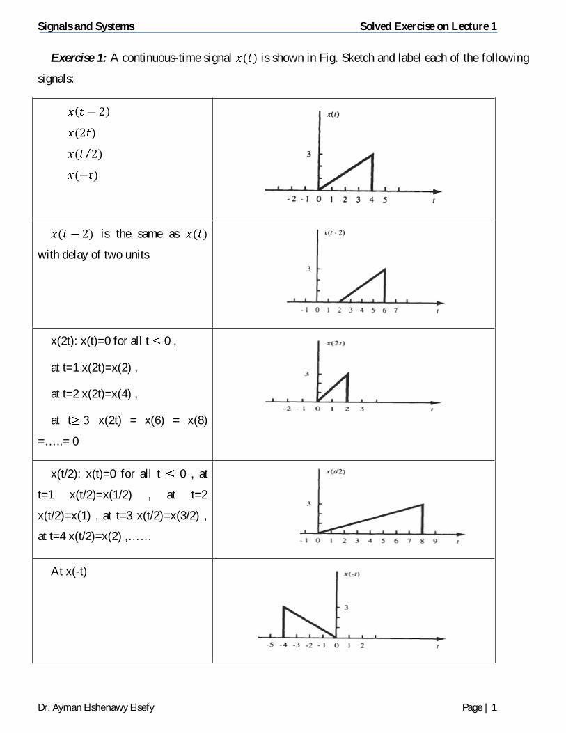
Exercise 1: A continuous-time signal is shown in Fig. Sketch and label each of the following
signals:
is the same as
with delay of two units
x(2t): x(t)=0 for all t 0 ,
at t=1 x(2t)=x(2) ,
at t=2 x(2t)=x(4) ,
at t x(2t) = x(6) = x(8)
=…..= 0
x(t/2): x(t)=0 for all t 0 , at
t=1 x(t/2)=x(1/2) , at t=2
x(t/2)=x(1) , at t=3 x(t/2)=x(3/2) ,
at t=4 x(t/2)=x(2) ,……
At x(-t)
Signals and Systems Solved Exercise on Lecture 1
Dr. Ayman Elshenawy Elsefy Page | 2
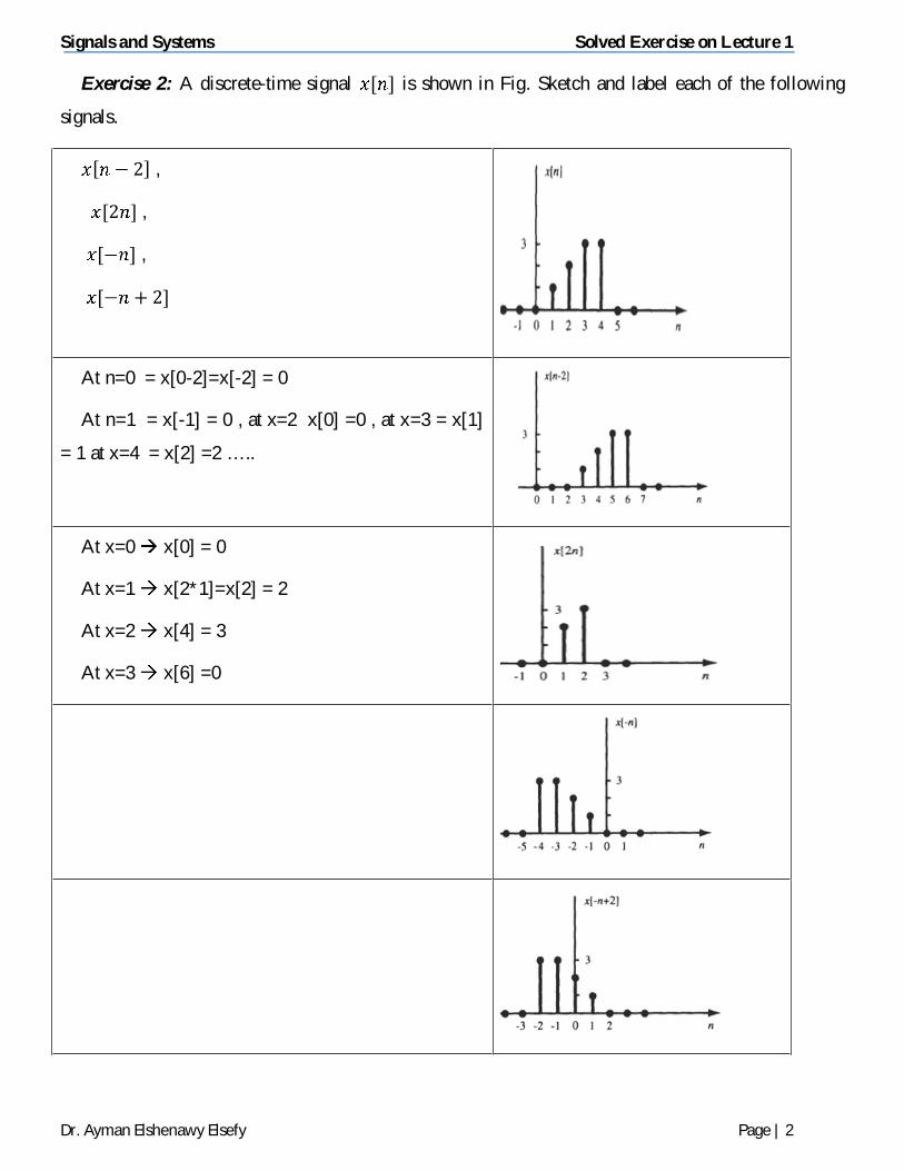
Exercise 2: A discrete-time signal is shown in Fig. Sketch and label each of the following
signals.
,
,
,
At n=0 = x[0-2]=x[-2] = 0
At n=1 = x[-1] = 0 , at x=2 x[0] =0 , at x=3 = x[1]
= 1 at x=4 = x[2] =2 …..
At x=0 x[0] = 0
At x=1 x[2*1]=x[2] = 2
At x=2 x[4] = 3
At x=3 x[6] =0
Signals and Systems Solved Exercise on Lecture 1
Dr. Ayman Elshenawy Elsefy Page | 3
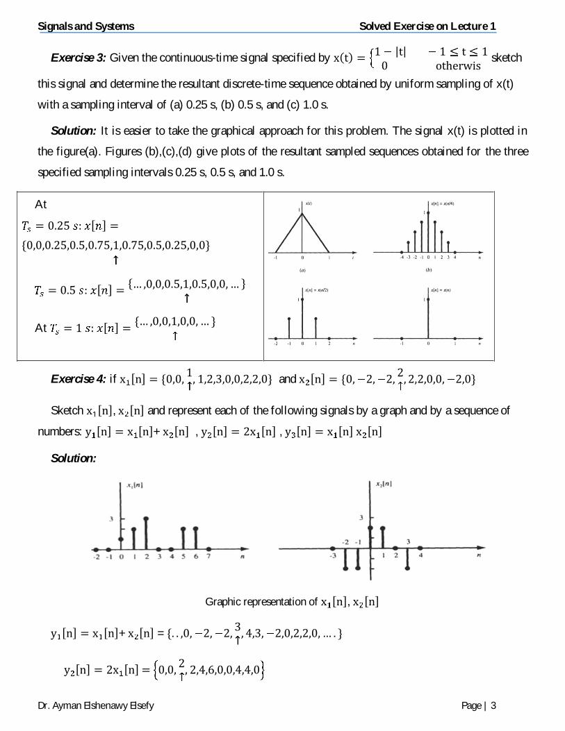
Exercise 3: Given the continuous-time signal specified by
sketch
this signal and determine the resultant discrete-time sequence obtained by uniform sampling of x(t)
with a sampling interval of (a) 0.25 s, (b) 0.5 s, and (c) 1.0 s.
Solution: It is easier to take the graphical approach for this problem. The signal x(t) is plotted in
the figure(a). Figures (b),(c),(d) give plots of the resultant sampled sequences obtained for the three
specified sampling intervals 0.25 s, 0.5 s, and 1.0 s.
At
At
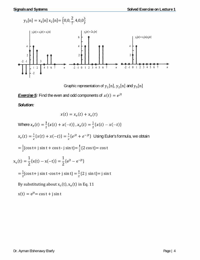
Exercise 4: if and
Sketch , and represent each of the following signals by a graph and by a sequence of
numbers: + , ,
Solution:
Graphic representation of ,
+ =
Signals and Systems Solved Exercise on Lecture 1
Dr. Ayman Elshenawy Elsefy Page | 4
Graphic representation of , and
Exercise 5: Find the even and odd components of
Solution:
Where
Using Euler's formula, we obtain
Signals and Systems Solved Exercise on Lecture 1
Dr. Ayman Elshenawy Elsefy Page | 5
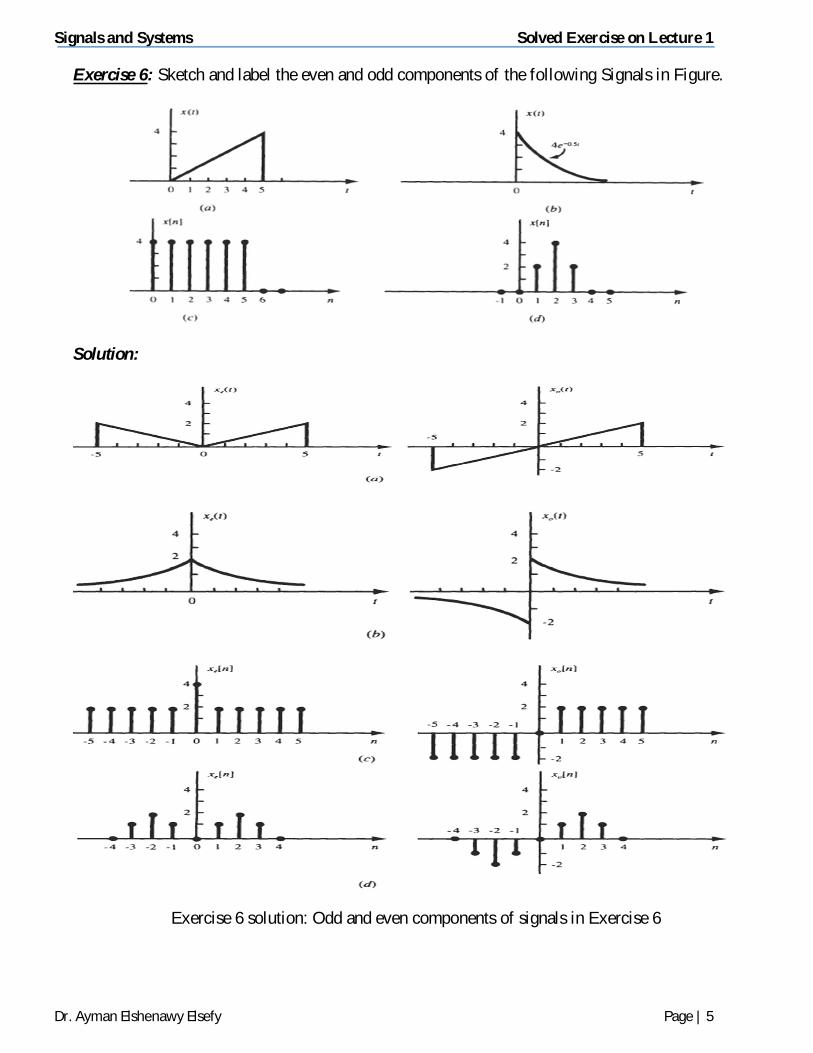
Exercise 6: Sketch and label the even and odd components of the following Signals in Figure.
Solution:
Exercise 6 solution: Odd and even components of signals in Exercise 6

Signals and Systems Solved Exercise on Lecture 1
Dr. Ayman Elshenawy Elsefy Page | 6
Exercise 7: Show that the complex exponential signal is periodic and that its
fundamental period is = .
Solution: is a periodic signal if
This can be achieved if
If then and is periodic.
If then only if or , if m=1 thus the fundamental period of
is .
Exercise 8: Show that the complex sinusoidal signal is periodic and that its
fundamental period is .
Solution: The sinusoidal signal is aperiodic signal if:
= = can be achieved only if
if or as in Ex. 5.
Exercise 9: Determine whether or not each of the following signals is periodic. If a signal is
periodic, determine its fundamental period.
Solution:
(a) is a sinusoidal signal in the form where and
The fundamental period
is periodic and The fundamental period .

Signals and Systems Solved Exercise on Lecture 1
Dr. Ayman Elshenawy Elsefy Page | 7
(b) Try to solve it as in the section (a)
(c)
Check the periodicity of and find the fundamental period
Check the periodicity of and find the fundamental period
Check If is rational number then is periodic signal.
(d) >>>> Try to solve it as in the section (c)
(e) = >>>> complete the solution as in section
(c) and (d).
(f) where
is aperiodic signal with fundamental period = , is constant and does not
affect the periodicity of .
Exercise 10: Determine whether the following are energy signals power signals, or neither
Solution:
(a)
Thus x(t) is an energy signal
(b) The sinusoidal signal x(t) is periodic with period with . the average power of x(t) is

Signals and Systems Solved Exercise on Lecture 1
Dr. Ayman Elshenawy Elsefy Page | 8
Thus x(t) is power signal, and in general periodic signals are power signal