Continuous similarity search for evolving queriesjpei/publications... · · 2016-06-06Continuous...

Knowl Inf SystDOI 10.1007/s10115-015-0892-x

REGULAR PAPER

Continuous similarity search for evolving queries

Xiaoning Xu1 · Chuancong Gao2 · Jian Pei2,3 ·Ke Wang2 · Abdullah Al-Barakati3

Received: 14 May 2015/Revised: 3 August 2015/Accepted: 5 October 2015© Springer-Verlag London 2015

Abstract In this paper, we study a novel problem of continuous similarity search for evolvingqueries. Given a set of objects, each being a set or multiset of items, and a data stream, wewant to continuously maintain the top-k most similar objects using the last n items in thestream as an evolving query. We show that the problem has several important applications.At the same time, the problem is challenging. We develop a filtering-based method and ahashing-based method. Our experimental results on both real data sets and synthetic data setsshow that our methods are effective and efficient.

Keywords Similarity search · Data stream · Evolving query

1 Introduction

Let us consider a recommendation problem at a Q&A website. Suppose you want to run 3 adson the Q&A website, for a user who does not have a profile yet, what ads should you display?In addition to many factors, such as click-through rates of ads and bidding price information,a natural and important idea is to consider the ads that are most related to the questions beingrecently asked at the website by all users. For example, technically, you may model ads andquestions as sets of keywords, and may want to retrieve the top-k ads that are most similar to

This work is partly supported by an NSERC Discovery grant, the Canada Research Chair program, and aYahoo! Faculty Research and Engagement Program (FREP) award. All opinions, findings, conclusions andrecommendations in this paper are those of the authors and do not necessarily reflect the views of thefunding agencies.

B Jian [email protected]

1 Fortinet Inc., Burnaby, BC, Canada

2 Simon Fraser University, Burnaby, BC, Canada

3 King Abdulaziz University, Jeddah, Saudi Arabia

123

http://crossmark.crossref.org/dialog/?doi=10.1007/s10115-015-0892-x&domain=pdf

X. Xu et al.

the last n questions asked, where the similarity measure captures the relevance between adsand questions. Such ads can be used as the candidates for further selections.

The above scenario is just one of the many applications that motivate the problem to bestudied in this paper. Given a set of static data objects (e.g., ads in the above example), and anevolving data stream (e.g., the questions asked in the above example), a sliding window onthe data stream (e.g., the last n questions in the above example) presents an evolving query.The problem of continuous similarity search for evolving queries is to continuously conducttop-k similarity search on the set of static objects using the evolving queries.

The problem of continuous similarity search for evolving queries has many importantapplications. As another example, in a computer role-playing game, a player has a set ofweapons and tools, which is relatively stable. The player goes through a game mission scene,where the objects in the continuously updated surrounding environment, such as differenttypes of enemies, scoring opportunities and obstacles, present a stream. The window overthe stream containing the most recent objects approaching the player presents an evolvingquery. The player has to select proper weapons and tools that match the current surroundingenvironment best. Here, an enemy can be modeled as a set of factors, such as explosion,that it may be tackled, and a weapon/tool can be modeled as a set of factors that it may beused. Again, before any gaming strategies can be used, an essential task is to continuouslymaintain the top-k best weapons and tools with respect to the evolving enemies.

Our problem can be considered as the dynamic version of the top-k set similarity searchproblem. More generally, a traditional similarity search problem involves a collection ofobjects, a similarity function, and a user-defined threshold. The search is to find all objectsin the collection whose similarity scores regarding the query are no less than the predefinedthreshold. Similarity search has many applications, such as information retrieval [14,16,33],near-duplicate web page detection [19], record linkage [37], data compression [16], dataintegration [9], image and video search and recommendation [13,15,31,35], statistics anddata analysis [12,22], machine learning [10], and data mining [3,18]. Besides answeringthreshold-based queries, top-k queries are also of great value since given a threshold, thesize of the result may be unpredictable and, in many real applications, we are only inter-ested in a small number of most similar objects. Moreover, as to be reviewed in Sect. 2.2,the problem of similarity search on data streams has been extensively explored, espe-cially for nearest neighbor search. However, to the best of our knowledge, the problemof continuous set-based similarity search for evolving queries has not been systematicallyinvestigated.

In this paper, we tackle the problem of continuous similarity search for evolving queries.Since in many applications, an object can be represented as a set or multiset, such as using akeyword vector to represent a document, we use weighted Jaccard similarity as the measure.The major challenge is how to speed up the similarity computation and avoid checking evolv-ing queries with every static object exactly at every time point. We develop an upper boundfor incremental maintenance of similarity scores. The bound can be computed in constanttime. We propose two algorithms, an exact one based on the pruning and verification frame-work, and the other approximate one based on MinHash. We report an empirical evaluationon both synthetic and real-world data sets, which validates the efficiency and effectivenessof our proposed methods.

The rest of the paper is organized as follows. In Sect. 2, we review the related work. Wethen formulate the problem in Sect. 3. In sect. 4, we propose a filtering-based method. InSect. 5, we present a hashing-based method. We report our experimental results in Sect. 6and conclude the paper in Sect. 7.

123


2 Related work

Our study is mainly related to the existing work on similarity search and continuous top-kqueries. In this section, we briefly review the state-of-the-art methods related to our study. Athorough survey on those topics is far beyond the capacity of the paper.

2.1 Similarity join and search

The static version of similarity search has been studied extensively. The state-of-the-artmethods can be categorized into two major groups.

The first category is the filtering-based approaches. The general idea is to develop upperand lower bounds of the similarity between an object and a query, which can be computedefficiently. Many objects can be filtered out using the bounds. Consequently, the exact simi-larity scores, which are supposed to be more expensive to compute, are calculated for onlya small number of surviving objects from filtering.

For instance, Sarawagi and Kirpal [34] proposed an inverted index-based probing methodfor similarity joins on sets. Chaudhuri et al. [8] developed the prefix-filtering principle forsimilarity joins. The all-pairs algorithm developed by Bayardo et al. [3] further improves thisapproach by adding the minimum length constraint and some other filtering techniques tospeed up similarity joins. Nevertheless, all-pairs and prefix-filtering methods often generate anontrivial number of candidates, which have to be verified using the exact similarity measure.Xiao et al. [38] extended the all-pairs method and proposed a new positional filtering methodPPJoin, which makes use of the ordering information. PPJoin+ [38] combines suffix filteringwith PPJoin and can further reduce the number of candidate pairs. A new similarity measurePathSim, which is based on meta path and is used in heterogeneous networks, is defined in[36].

The second category is hashing-based methods. The general idea is to develop hash func-tions that have good locality preservation properties—similar objects are likely to be hashedto the same bucket. The idea was introduced by Indyk and Motwani [21] for approximatenearest neighbor search in d-dimensional Euclidean space. The basic principle is to hashthe points using multiple hash functions such that closer points have a higher probability ofcollision than points that are far away. Gionis et al. [17] further improved the algorithms andachieved better query time guarantees. Later, an improved algorithm that almost achievesthe space and time lower bounds is presented by Andoni and Indyk [1]. The MinHash tech-nique [5] is used to approximate the resemblance and the containment of sets. This techniqueis used to estimate the rarity and similarity between two windowed data streams in [11]. More-over, Charikar [7] proposed SimHash to hash similar data to similar values. An estimationfor vector-based cosine similarity using a random projection method is also discussed [7].

In this paper, we explore both filtering-based and hashing-based methods, which have notbeen addressed in the existing literature for evolving similarity search queries.

2.2 Continuous queries over a data stream

Different evolving models are used in previous studies that investigated continuous queriesover a data stream. For example, Kontaki et al. [24] studied similarity range queries instreaming time sequences using Euclidean distance, where both the query and data objectsare evolving. An indexing method that is based on incremental computation method fordiscrete Fourier transform is used to achieve a high candidates ratio. Lian et al. [26] tackledthe similarity search problem over multiple stream time series, given a static time series as a

123

X. Xu et al.

query. An approximation algorithm is developed using a weighted locality-sensitive hashingtechnique.

Motivated by a wide range of applications such as network intrusion detection, muchwork [4,25,28,29] has been embarked on monitoring nearest neighbor (NN) queries contin-uously over a data stream. The basic idea is to utilize indexing structures for reducing memoryconsumption and supporting efficient updates. Mouratidis et al. [28] proposed two approachesfor continuous monitoring of NN queries over sliding window streams. Koudas et al. [25]developed an approximation algorithm that utilizes an indexing scheme, DISC, and has guar-anteed bounds on error and performance.

The existing work on continuously monitoring nearest neighbors for mobile query objectis different from the problem studied here. In those previous studies, the mobile object isassumed to move in a trajectory, potentially predictable to some extent. In this paper, thestream presenting an evolving query is not assumed a moving object. Instead, we simply usethe current sliding window as the current query. The existing methods on continuous nearestneighbor monitoring for mobile objects cannot solve our problem.

In addition to continuous queries on similarity search problems, some interesting problemsare defined over data streams. For example, Pan and Zhu [30] developed a two-level candidatechecking scheme for continuously querying the top-k correlated graphs in a data streamscenario where static queries are posed on evolving graph streams. Mouratidis et al. [27]proposed two approaches for continuously answering top-k queries where the query is astatic preference function over a fixed-size sliding window. One approach is to compute newanswers whenever a current top-k point expired and the other approach is to precompute futurechanges partially. Rao et al. [32] devised methods for the problem that uses an aggregationfunction to measure the relevance between a document stream and a query consists of terms.They modeled documents as a data stream. That is, new documents keep coming while thequery is not evolving, which is different from our model where the evolving query consistsof the elements in the current sliding window in a data stream. Kollios and Tsotras [23]proposed efficient hashing methods to answer membership queries in a temporal setting.

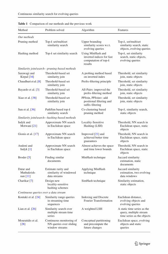
Table 1 summarizes the differences between our study and some previous methods relatedto ours.

3 Problem definition

Let us consider an alphabet of items �, a collection of objects R where each object is a set(or multiset) over �, a data stream S with each element e ∈ � keeps coming, and an integern as the size of a query sliding window on S. A query Q is the last n elements in S. A queryis in general a multiset, but also can be modeled as a set. The top-k continuous similaritysearch for evolving query Q is to continuously find the k objects in R that are most similarto Q. We answer the query continuously whenever a new element in S arrives.

In this paper, we consider each object being a set or multiset. Queries can be sets ormultisets as well. Since a set is a special case of a multiset where elements in the object areall distinct, we use weighted Jaccard similarity to measure the similarity between objects andqueries.

Specifically, let X be a nonempty multiset that consists of items in alphabet � ={v1, v2, . . . , v|�|}. We map X to a |�|-dimensional vector �X such that the value of thei th component is the absolute frequency of item vi in X . �X is called the vector representationof multiset X .

123


Table 1 Comparison of our methods and the previous work

Method Problem solved Algorithm Features

Our methods

Pruning method Top-k set/multisetsimilarity search

Upper boundingsimilarity scores w.r.t.evolving queries

Top-k, set/multisetsimilarity search, staticobjects, evolving queries

Hashing method Top-k set similarity search Using MinHash andinverted indices for fastcomputation of top-kresults

Top-k, set similaritysearch, static objects,evolving queries

Similarity join/search—pruning-based methods

Sarawagi andKirpal [34]

Threshold-based setsimilarity join

A probing method basedon inverted index

Threshold, set similarityjoin, static objects

Chaudhuri et al. [8] Threshold-based setsimilarity join

Prefix-filtering principle Threshold, set similarityjoin, static objects

Bayardo et al. [3] Threshold-based setsimilarity join

All-Pairs: improved theprefix-filtering method


Xiao et al. [38] Threshold-based setsimilarity join

PPJoin, PPJoin+: addpositional filtering andsuffix filtering


Sun et al. [36] PathSim based top-ksimilarity search

Co-clustering basedpruning method

Top-k, similarity search,static objects

Similarity join/search—hashing-based methods

Indyk andMotwani [21]

Approximate NN searchin Euclidean space

Locality-SensitiveHashing (LSH)

Threshold, NN search inEuclidean space, staticobjects

Gionis et al. [17] Approximate NN searchin Euclidean space

Improved [21] andachieved better timeguarantees


Andoni andIndyk [1]

Approximate NN searchin Euclidean space

Almost achieves the spaceand time lower bounds


Broder [5] Finding similardocuments

MinHash technique Jaccard similarityestimation, staticdocuments

Datar andMuthukrish-nan [11]

Estimate rarity andsimilarity of windoweddata streams

Applying MinHashtechnique

Jaccard similarityestimation, two evolvingdata windows

Charikar [7] Design newlocality-sensitivehashing schemes

SimHash technique Similarity estimation,static objects

Continuous queries over a data stream

Kontaki et al. [24] Similarity range queriesin streaming timesequences

Indexing and DiscreteFourier Transformation

Euclidean distance,evolving objects andevolving queries

Lian et al. [26] Similarity search overmultiple stream timeseries

A weighted LSH A static time series as thequery, multiple streamtime series as the objects

Mouratidis et al.[28]

Continuous monitoring ofNN queries over slidingwindow streams

Conceptual partitioningand precompute thefuture changes

Euclidean space, evolvingobjects and staticqueries

123

X. Xu et al.

Table 1 continued

Method Problem solved Algorithm Features

Pan and Zhu [30] Continuously queryingthe top-k correlatedgraphs in a data stream

A two-level candidatechecking scheme

Evolving graph streamsand static queries

Rao et al. [32] Measure the relevancebetween a documentstream and a query

A graph indexingstructure for resultssharing among queries

Evolving documents andstatic queries

Table 2 A collection of sets RT1 a b c f i

T2 a d e

T3 d e

T4 b c d i

T5 a c g h i j

T6 a c e f h

· · · b i c a d ←−(a)

· · · b i c a d f ←−(b)

Fig. 1 Query stream S. a Current query Q, b query Q′ after a new item arrives

Let X and Y be two nonempty multisets over alphabet �. Let �X = [x1, x2, . . . , x|�|] and�Y = [y1, y2, . . . , y|�|] be the vector representations of X and Y , respectively. The weightedJaccard similarity is

sim jac(X, Y ) = sim jac( �X , �Y ) =∑|�|

i=1 min(xi , yi )∑|�|

i=1 max(xi , yi )(1)

Example 1 (Computing similarity scores) Given an alphabet � = {a, b, c, d, e, f, g}, con-sider two multisets X = {c, b, a, e, f } and Y = {a, b, a, c, e, d}. The vector representationsof X and Y are �x = [1, 1, 1, 0, 1, 1, 0] and �y = [2, 1, 1, 1, 1, 0, 0], respectively. Since∑7

i=1 max(xi , yi ) = 7 and∑7

i=1 min(xi , yi ) = 4, the weighted Jaccard similarity scorebetween X and Y is sim jac(X, Y ) = 4

7 = 0.57.

We now model how a query evolves. Given a query Q = {ep+1, ep+2, . . . , ep+|Q|},where item ep+i (1 ≤ i ≤ |Q|) is the i-th arrived item in the query, the updatedquery after u time instants (u ≤ |Q|), that is, u updates in the stream, is Q′ ={ep+u+1, ep+u+2, . . . , ep+|Q|, ep+|Q|+1, ep+|Q|+2, . . . , ep+|Q|+u}, where item ep+|Q|+ j isthe j-th newly coming element in the updated query, 1 ≤ j ≤ u.

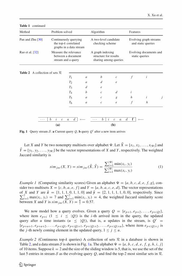
Example 2 (Continuous top-k queries) A collection of sets R in a database is shown inTable 2, and a data stream S is shown in Fig. 1a. The alphabet � = {a, b, c, d, e, f, g, h, i, j}of 10 items. Suppose k = 2 and the size of the sliding window is 5, that is, we use the set of thelast 5 entries in stream S as the evolving query Q, and find the top-2 most similar sets in R.

123


Table 3 Jaccard similarityscores

T1 T2 T3 T4 T5 T6

Q 0.67 0.33 0.17 0.80 0.38 0.25

Q′ 0.67 0.33 0.17 0.50 0.38 0.43

Table 4 Summary of frequently used symbols

Symbol Interpretation

For all methods

R A collection of objects in database

S The querying data stream

� The alphabet used in database

Ti The i th object in RQt The query containing the elements in the sliding window at time t

�X The vector representation of a set (or multiset) X

sim(X, Y ) The exact similarity of two sets (or multisets) X and Y

k Number of objects in the result

topkt The k objects that are most similar to the query at time t

score(topkt [k]) The similarity score of the kth most similar result at time t

For pruning-based method

sim(X, Y )+u The upper bound of similarity score of two sets (or multisets) X and Y , after uupdates on Y

min_stepi The least number of updates needed for object Ti ’s progressive upper boundsim(Ti , Qt )+min_stepi to exceed score(topkt [k])

For MinHash-based method

{[n]} The set {0, . . . , n − 1}sim≈(X, Y ) The MinHash approximated similarity of two sets X and Y

H A set of hash functions h1, h2, . . . , h|H |indexi Inverted index built on the MinHash values of the i th hash function, i ∈ [1, |H |]indexi [v] Inverted list of hash value v which consists of the objects whose MinHash value is

v according to the i th hash function, i ∈ [1, |H |] and v ∈ [1, |�|]min(hi (X)) The minimum hash (MinHash) value of set X according to the i th hash function

hi , i ∈ [1, |H |]For experiments

|Q̄t | The average object length of the data set

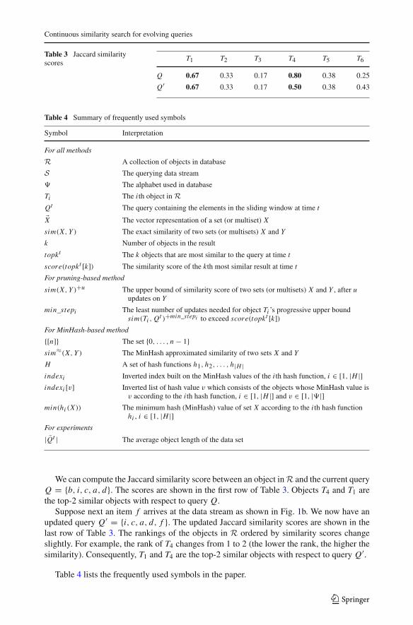
We can compute the Jaccard similarity score between an object in R and the current queryQ = {b, i, c, a, d}. The scores are shown in the first row of Table 3. Objects T4 and T1 arethe top-2 similar objects with respect to query Q.

Suppose next an item f arrives at the data stream as shown in Fig. 1b. We now have anupdated query Q′ = {i, c, a, d, f }. The updated Jaccard similarity scores are shown in thelast row of Table 3. The rankings of the objects in R ordered by similarity scores changeslightly. For example, the rank of T4 changes from 1 to 2 (the lower the rank, the higher thesimilarity). Consequently, T1 and T4 are the top-2 similar objects with respect to query Q′.

Table 4 lists the frequently used symbols in the paper.

123

X. Xu et al.

4 A pruning-based method

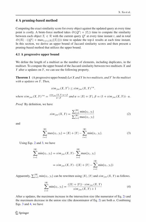
Computing the exact similarity score for every object against the updated query at every timepoint is costly. A brute-force method takes O(|Qt | + |Ti |) time to compute the similaritybetween each object Ti ∈ R with the current query Qt at every time instant t , and in totalO(|R| · (|Qt | + max1≤i≤|R|{|Ti |})) time to update the top-k results at each time instant.In this section, we derive an upper bound of Jaccard similarity scores and then present apruning-based method that utilizes the upper bound.

4.1 A progressive upper bound

We define the length of a multiset as the number of elements, including duplicates, in themultiset. To compute the upper bound of the Jaccard similarity between two multisets X andY after u updates on Y , we can use the following property.

Theorem 1 (A progressive upper bound) Let X and Y be two multisets, and Y ′ be the multisetwith u updates on Y . Then,

sim jac(X, Y ′) ≤ sim jac(X, Y )+u .

where sim jac(X, Y )+u = sim jac(X,Y )·α+β

α−βand α = |X | + |Y |, β = (1 + sim jac(X, Y )) · u.

Proof By definition, we have

sim jac(X, Y ) =∑|�|

i=1 min{xi , yi }∑|�|

i=1 max{xi , yi }(2)

and

|�|∑

i=1

max{xi , yi } = |X | + |Y | −|�|∑

i=1

min{xi , yi }. (3)

Using Eqs. 2 and 3, we have

|�|∑

i=1

min{xi , yi } = sim jac(X, Y ) ·|�|∑

i=1

max{xi , yi }

= sim jac(X, Y ) · (|X | + |Y | −|�|∑

i=1

min{xi , yi })

Apparently,∑|�|

i=1 min{xi , yi } can be rewritten using |X |, |Y | and sim jac(X, Y ) as follows.

|�|∑

i=1

min{xi , yi } = (|X | + |Y |) · sim jac(X, Y )

sim jac(X, Y ) + 1(4)

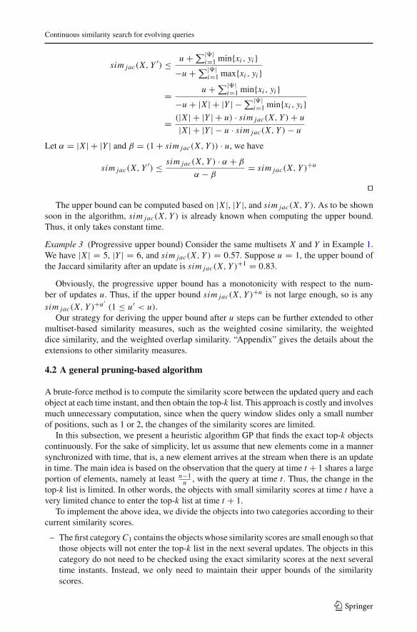
After u updates, the maximum increase in the intersection size (the numerator of Eq. 2) andthe maximum decrease in the union size (the denominator of Eq. 2) are both u. CombiningEqs. 3 and 4, we have

123


sim jac(X, Y ′) ≤ u + ∑|�|i=1 min{xi , yi }

−u + ∑|�|i=1 max{xi , yi }

= u + ∑|�|i=1 min{xi , yi }

−u + |X | + |Y | − ∑|�|i=1 min{xi , yi }

= (|X | + |Y | + u) · sim jac(X, Y ) + u

|X | + |Y | − u · sim jac(X, Y ) − u

Let α = |X | + |Y | and β = (1 + sim jac(X, Y )) · u, we have

sim jac(X, Y ′) ≤ sim jac(X, Y ) · α + β

α − β= sim jac(X, Y )+u

��The upper bound can be computed based on |X |, |Y |, and sim jac(X, Y ). As to be shown

soon in the algorithm, sim jac(X, Y ) is already known when computing the upper bound.Thus, it only takes constant time.

Example 3 (Progressive upper bound) Consider the same multisets X and Y in Example 1.We have |X | = 5, |Y | = 6, and sim jac(X, Y ) = 0.57. Suppose u = 1, the upper bound ofthe Jaccard similarity after an update is sim jac(X, Y )+1 = 0.83.

Obviously, the progressive upper bound has a monotonicity with respect to the num-ber of updates u. Thus, if the upper bound sim jac(X, Y )+u is not large enough, so is anysim jac(X, Y )+u′

(1 ≤ u′ < u).Our strategy for deriving the upper bound after u steps can be further extended to other

multiset-based similarity measures, such as the weighted cosine similarity, the weighteddice similarity, and the weighted overlap similarity. “Appendix” gives the details about theextensions to other similarity measures.

4.2 A general pruning-based algorithm

A brute-force method is to compute the similarity score between the updated query and eachobject at each time instant, and then obtain the top-k list. This approach is costly and involvesmuch unnecessary computation, since when the query window slides only a small numberof positions, such as 1 or 2, the changes of the similarity scores are limited.

In this subsection, we present a heuristic algorithm GP that finds the exact top-k objectscontinuously. For the sake of simplicity, let us assume that new elements come in a mannersynchronized with time, that is, a new element arrives at the stream when there is an updatein time. The main idea is based on the observation that the query at time t + 1 shares a largeportion of elements, namely at least n−1

n , with the query at time t . Thus, the change in thetop-k list is limited. In other words, the objects with small similarity scores at time t have avery limited chance to enter the top-k list at time t + 1.

To implement the above idea, we divide the objects into two categories according to theircurrent similarity scores.

– The first category C1 contains the objects whose similarity scores are small enough so thatthose objects will not enter the top-k list in the next several updates. The objects in thiscategory do not need to be checked using the exact similarity scores at the next severaltime instants. Instead, we only need to maintain their upper bounds of the similarityscores.

123

X. Xu et al.

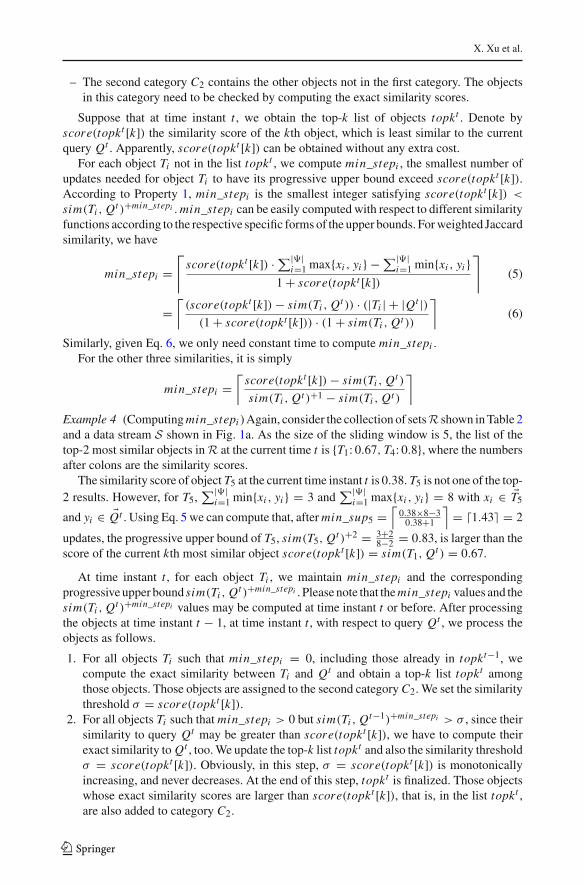
– The second category C2 contains the other objects not in the first category. The objectsin this category need to be checked by computing the exact similarity scores.

Suppose that at time instant t , we obtain the top-k list of objects topkt . Denote byscore(topkt [k]) the similarity score of the kth object, which is least similar to the currentquery Qt . Apparently, score(topkt [k]) can be obtained without any extra cost.

For each object Ti not in the list topkt , we compute min_stepi , the smallest number ofupdates needed for object Ti to have its progressive upper bound exceed score(topkt [k]).According to Property 1, min_stepi is the smallest integer satisfying score(topkt [k]) <

sim(Ti , Qt )+min_stepi . min_stepi can be easily computed with respect to different similarityfunctions according to the respective specific forms of the upper bounds. For weighted Jaccardsimilarity, we have

min_stepi =⌈

score(topkt [k]) · ∑|�|i=1 max{xi , yi } − ∑|�|

i=1 min{xi , yi }1 + score(topkt [k])

⌉

(5)

=⌈

(score(topkt [k]) − sim(Ti , Qt )) · (|Ti | + |Qt |)(1 + score(topkt [k])) · (1 + sim(Ti , Qt ))

⌉

(6)

Similarly, given Eq. 6, we only need constant time to compute min_stepi .For the other three similarities, it is simply

min_stepi =⌈

score(topkt [k]) − sim(Ti , Qt )

sim(Ti , Qt )+1 − sim(Ti , Qt )

⌉

Example 4 (Computing min_stepi ) Again, consider the collection of setsR shown in Table 2and a data stream S shown in Fig. 1a. As the size of the sliding window is 5, the list of thetop-2 most similar objects in R at the current time t is {T1: 0.67, T4: 0.8}, where the numbersafter colons are the similarity scores.

The similarity score of object T5 at the current time instant t is 0.38. T5 is not one of the top-2 results. However, for T5,

∑|�|i=1 min{xi , yi } = 3 and

∑|�|i=1 max{xi , yi } = 8 with xi ∈ �T5

and yi ∈ �Qt . Using Eq. 5 we can compute that, after min_sup5 =⌈

0.38×8−30.38+1

⌉= 1.43 = 2

updates, the progressive upper bound of T5, sim(T5, Qt )+2 = 3+28−2 = 0.83, is larger than the

score of the current kth most similar object score(topkt [k]) = sim(T1, Qt ) = 0.67.

At time instant t , for each object Ti , we maintain min_stepi and the correspondingprogressive upper bound sim(Ti , Qt )+min_stepi . Please note that the min_stepi values and thesim(Ti , Qt )+min_stepi values may be computed at time instant t or before. After processingthe objects at time instant t − 1, at time instant t , with respect to query Qt , we process theobjects as follows.

1. For all objects Ti such that min_stepi = 0, including those already in topkt−1, wecompute the exact similarity between Ti and Qt and obtain a top-k list topkt amongthose objects. Those objects are assigned to the second category C2. We set the similaritythreshold σ = score(topkt [k]).

2. For all objects Ti such that min_stepi > 0 but sim(Ti , Qt−1)+min_stepi > σ , since theirsimilarity to query Qt may be greater than score(topkt [k]), we have to compute theirexact similarity to Qt , too. We update the top-k list topkt and also the similarity thresholdσ = score(topkt [k]). Obviously, in this step, σ = score(topkt [k]) is monotonicallyincreasing, and never decreases. At the end of this step, topkt is finalized. Those objectswhose exact similarity scores are larger than score(topkt [k]), that is, in the list topkt ,are also added to category C2.

123


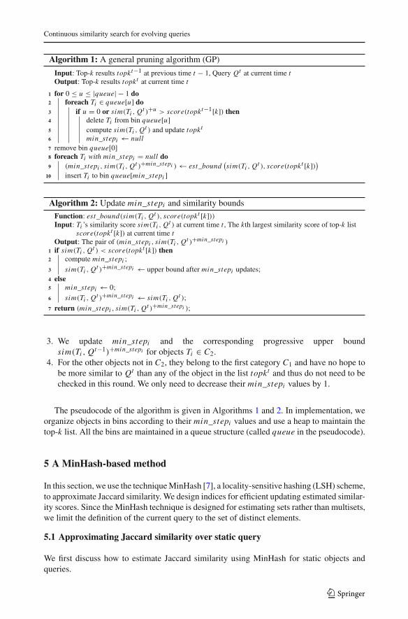
Algorithm 1: A general pruning algorithm (GP)

Input: Top-k results topkt−1 at previous time t − 1, Query Qt at current time tOutput: Top-k results topkt at current time t

1 for 0 ≤ u ≤ |queue| − 1 do2 foreach Ti ∈ queue[u] do3 if u = 0 or sim(Ti , Qt )+u > score(topkt−1[k]) then4 delete Ti from bin queue[u]5 compute sim(Ti , Qt ) and update topkt

6 min_stepi ← null7 remove bin queue[0]8 foreach Ti with min_stepi = null do9 (min_stepi , sim(Ti , Qt )+min_stepi ) ← est_bound

(sim(Ti , Qt ), score(topkt [k]))

10 insert Ti to bin queue[min_stepi ]

Algorithm 2: Update min_stepi and similarity bounds

Function: est_bound(sim(Ti , Qt ), score(topkt [k]))Input: Ti ’s similarity score sim(Ti , Qt ) at current time t , The kth largest similarity score of top-k list

score(topkt [k]) at current time tOutput: The pair of (min_stepi , sim(Ti , Qt )+min_stepi )

1 if sim(Ti , Qt ) < score(topkt [k]) then2 compute min_stepi ;

3 sim(Ti , Qt )+min_stepi ← upper bound after min_stepi updates;4 else5 min_stepi ← 0;

6 sim(Ti , Qt )+min_stepi ← sim(Ti , Qt );

7 return (min_stepi , sim(Ti , Qt )+min_stepi );

3. We update min_stepi and the corresponding progressive upper boundsim(Ti , Qt−1)+min_stepi for objects Ti ∈ C2.

4. For the other objects not in C2, they belong to the first category C1 and have no hope tobe more similar to Qt than any of the object in the list topkt and thus do not need to bechecked in this round. We only need to decrease their min_stepi values by 1.

The pseudocode of the algorithm is given in Algorithms 1 and 2. In implementation, weorganize objects in bins according to their min_stepi values and use a heap to maintain thetop-k list. All the bins are maintained in a queue structure (called queue in the pseudocode).

5 A MinHash-based method

In this section, we use the technique MinHash [7], a locality-sensitive hashing (LSH) scheme,to approximate Jaccard similarity. We design indices for efficient updating estimated similar-ity scores. Since the MinHash technique is designed for estimating sets rather than multisets,we limit the definition of the current query to the set of distinct elements.

5.1 Approximating Jaccard similarity over static query

We first discuss how to estimate Jaccard similarity using MinHash for static objects andqueries.

123

X. Xu et al.

Definition 1 (Image under permutation [2]) Denote by {[n]} the set {0, . . . , n − 1}. A per-mutation π on {[n]} is a bijective function (one-to-one correspondence) from {[n]} to itself.If x ∈ {[n]}, then π(x), the value of π when applied to x is the image of x under π . Theimage of a subset X ⊆ [n] under π is π [X ] = {y | y = π(x) for x ∈ X}.Definition 2 (Min-wise independent permutations [6]) Let Sn be the set of all permutationsof {[n]}. A family of permutations F ⊆ Sn is min-wise independent if for any set X ⊆ {[n]}and any element x ∈ X , we have

Pr(min{π [X ]} = π(x)) = 1

|X | (7)

where the permutation π is chosen randomly in F .

The following property enables efficient estimation of Jaccard similarity between twosets.

Theorem 2 (Jaccard similarity estimation [20]) Consider a query Q and an object Ti wherethe elements are drawn from an alphabet �. Let h be a hash function that maps elements in� to distinct integers in range [0, |�|− 1] and is randomly picked from a family of min-wiseindependent permutations. Let the MinHash value, min(h(Ti )), be the element in Ti with thesmallest hash value. Then, Pr [min(h(Ti )) = min(h(Q))] = |Ti ∩Q|

|Ti ∪Q| .

The MinHash values for all objects and that of the query can be stored in a MinHashsignature matrix, M , where each entry M(i, j) is the MinHash value of the j th itemsetunder hash function hi . Based on Property 2, the Jaccard similarity between two sets canbe estimated by the ratio of the number of rows containing the same MinHash values to thenumber of all the rows in the signature matrix. We deliberate the computation in Example 5.

Example 5 (Jaccard similarity estimation) Consider the matrix representation of an examplewith four objects and a static query Q shown in Table 5a. Each column in the matrix representsa set and an element is in the set if the corresponding entry is 1. We apply five randompermutations defined in Table 5b as the min-wise independent hash functions on objectsand the query. The signature matrix is shown in Table 5c. For example, since object T1

contains elements a, b, and c, the corresponding hash values according to h4 are 1, 3, and 4,respectively. The MinHash value of T1 according to h4 is a since a is the element in T1 withthe smallest hash value.

We can estimate the Jaccard similarity score between two sets by computing the ratio of thenumber of rows containing the same MinHash values to the number of random permutations.For example, the MinHash values of T1 and Q are the same according to random permutationsh2 and h3. Thus, the estimated Jaccard similarity between T1 and Q is 2

5 . We compare theestimated Jaccard similarity with the exact Jaccard similarity for each object in Table 5d.When objects are ordered in descending order of estimated similarity score regarding to thequery, we have T3 > T1 = T4 > T2, which is identical to the order using exact similarity.Therefore, in this example, we can get the top-k result accurately using estimated scores.

5.2 Approximating Jaccard similarity over evolving query

To answer evolving queries, given a fixed set of hash functions, the MinHash values for allthe objects are fixed and only the MinHash values for the query are subject to modification.That is, we only need to update the MinHash values for the query. Therefore, we have a fastsolution shown in Algorithm 3.

123


Table 5 An example of Jaccardsimilarity estimation

Element T1 T2 T3 T4 Q

(a) Matrix representation of sets

a 1 1 0 1 0

b 1 0 1 0 1

c 1 0 1 0 1

d 0 1 0 1 1

e 0 0 1 1 1

Element h1 h2 h3 h4 h5

(b) Random permutations

a 1 2 3 1 0

b 2 3 0 3 4

c 3 0 1 4 3

d 4 4 2 0 1

e 0 1 4 2 2

T1 T2 T3 T4 Q

(c) Signature matrix

h1 a a e e e

h2 c a c e c

h3 b d b d b

h4 a d e d d

h5 a a e a d

T1 T2 T3 T4

(d) Exact and approximated Jaccard similarity

sim jac(Ti , Q) 0.40 0.25 0.75 0.40

sim≈jac(Ti , Q) 0.40 0.20 0.60 0.40

Algorithm 3 first computes the MinHash signature for an updated query. To determinewhether we need to update the estimated Jaccard similarity of object Tj with respect to theupdated query Qt according to a hash function hi , we consider the following 4 cases basedon whether the MinHash values of the object and the queries are equal or not.

– Case 1: If min(hi (Tj )) �= min(hi (Qt−1)) and min(hi (Tj )) = min(hi (Qt )), the esti-mated Jaccard similarity between Tj and the updated query should be increased by 1

|H | ,where |H | is the number of hash functions applied.

– Case 2: If min(hi (Tj )) = min(hi (Qt−1)) and min(hi (Tj )) �= min(hi (Qt )), the esti-mated Jaccard similarity between Tj and the updated query should be decreased by 1

|H | .– Case 3: If min(hi (Tj )) = min(hi (Qt−1)) and min(hi (Tj )) = min(hi (Qt )), the esti-

mated Jaccard similarity between Tj and the updated query remains.– Case 4: If min(hi (Tj )) �= min(hi (Qt−1)) and min(hi (Tj )) �= min(hi (Qt )), the esti-

mated Jaccard similarity between Tj and the updated query remains, too.

We can further reduce the computational cost using inverted indices. The MinHash sig-nature matrix that stores the MinHash values of objects can be transformed into |H | inverted

123

X. Xu et al.

Algorithm 3: A MinHash-based algorithm (MHB)

Input: Current query Qt , |H | hash functions, a set of previous MinHash values {min(hi (Qt−1))},MinHash table for |R| objects.

Output: Top-k results topkt at current time t1 compute {min(hi (Qt ))};2 foreach j ∈ {1, . . . , |R|} do3 foreach i ∈ {1, . . . , |H |} do4 if min(hi (Tj )) �= min(hi (Qt−1)) and min(hi (Tj )) = min(hi (Qt )) then5 sim≈(Tj , Qt ) ← sim(Tj , Qt ) + 1

|H | ;

6 else if min(hi (Tj )) = min(hi (Qt−1)) and min(hi (Tj )) �= min(hi (Qt )) then7 sim≈(Tj , Qt ) ← sim(Tj , Qt ) − 1

|H | ;

8 if Tj /∈ topkt and sim≈(Tj , Qt ) > score(topkt [k]) then9 update topkt ;

Fig. 2 Inverted indices for MinHash values

indices whose structure is shown in Fig. 2. For each hash function, its corresponding invertedindex stores a mapping from each existing MinHash value to a list of object ids, that is,inverted list. Moreover, elements in each inverted list are sorted in ascending order of objectid, which enables more efficient list merge and intersection operations. In this way, we canefficiently retrieve the objects with a specified MinHash value according to a certain hashfunction.

The algorithm that uses the inverted indices is presented in Algorithm 4. The MinHashsignature for the updated query is computed first. We need to search the inverted indexof a hash function hi only when the MinHash values of Qt and Qt−1 regarding hi aredifferent. Suppose the MinHash value of the updated query changes according to hi , todetermine the objects whose similarity scores need to be updated, we recall Case 1 and Case2 mentioned earlier in this section. Each case corresponds to a scan in an inverted list of hi .Specifically, in Case 1, we increase the estimated Jaccard similarity by 1

|H | for objects in theinverted list of hash value min(hi (Qt )). That is, instead of checking for each object as inAlgorithm 3, we search for the objects that satisfy Case 1 using the index. Similarly, in Case2, we decrease the estimated Jaccard similarity by 1

|H | for objects in the inverted list of hash

value min(hi (Qt−1)).

123


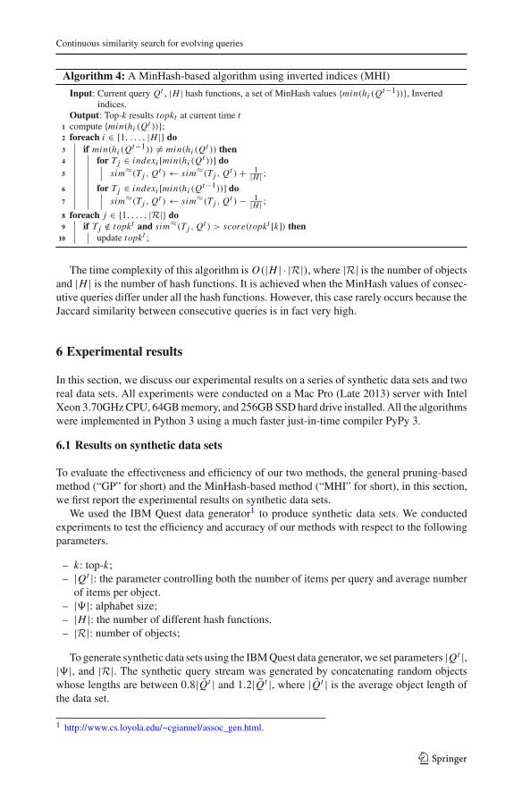
Algorithm 4: A MinHash-based algorithm using inverted indices (MHI)

Input: Current query Qt , |H | hash functions, a set of MinHash values {min(hi (Qt−1))}, Invertedindices.

Output: Top-k results topkt at current time t1 compute {min(hi (Qt ))};2 foreach i ∈ {1, . . . , |H |} do3 if min(hi (Qt−1)) �= min(hi (Qt )) then4 for Tj ∈ indexi [min(hi (Qt ))] do5 sim≈(Tj , Qt ) ← sim≈(Tj , Qt ) + 1

|H | ;

6 for Tj ∈ indexi [min(hi (Qt−1))] do7 sim≈(Tj , Qt ) ← sim≈(Tj , Qt ) − 1

|H | ;

8 foreach j ∈ {1, . . . , |R|} do9 if Tj /∈ topkt and sim≈(Tj , Qt ) > score(topkt [k]) then

10 update topkt ;

The time complexity of this algorithm is O(|H | · |R|), where |R| is the number of objectsand |H | is the number of hash functions. It is achieved when the MinHash values of consec-utive queries differ under all the hash functions. However, this case rarely occurs because theJaccard similarity between consecutive queries is in fact very high.

6 Experimental results

In this section, we discuss our experimental results on a series of synthetic data sets and tworeal data sets. All experiments were conducted on a Mac Pro (Late 2013) server with IntelXeon 3.70GHz CPU, 64GB memory, and 256GB SSD hard drive installed. All the algorithmswere implemented in Python 3 using a much faster just-in-time compiler PyPy 3.

6.1 Results on synthetic data sets

To evaluate the effectiveness and efficiency of our two methods, the general pruning-basedmethod (“GP” for short) and the MinHash-based method (“MHI” for short), in this section,we first report the experimental results on synthetic data sets.

We used the IBM Quest data generator1 to produce synthetic data sets. We conductedexperiments to test the efficiency and accuracy of our methods with respect to the followingparameters.

– k: top-k;– |Qt |: the parameter controlling both the number of items per query and average number

of items per object.– |�|: alphabet size;– |H |: the number of different hash functions.– |R|: number of objects;

To generate synthetic data sets using the IBM Quest data generator, we set parameters |Qt |,|�|, and |R|. The synthetic query stream was generated by concatenating random objectswhose lengths are between 0.8|Q̄t | and 1.2|Q̄t |, where |Q̄t | is the average object length ofthe data set.

1 http://www.cs.loyola.edu/~cgiannel/assoc_gen.html.

123

http://www.cs.loyola.edu/~cgiannel/assoc_gen.html

X. Xu et al.

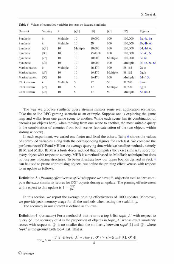
Table 6 Values of controlled variables for tests on Jaccard similarity

Data set Varying k |Qt | |�| |H | |R| Figures

Synthetic k Multiple 10 10,000 100 100,000 3a, 4a, 6a

Synthetic k Multiple 10 20 100 100,000 3b, 4b, 6b

Synthetic |Qt | 10 Multiple 10,000 100 100,000 3d, 4d, 6c

Synthetic |�| 10 10 Multiple 100 100,000 3c, 4c, 6c

Synthetic |H | 10 10 10,000 Multiple 100,000 3e, 6e

Synthetic |R| 10 10 10,000 100 Multiple 3f, 4e, 5a, 6f

Market basket k Multiple 10 16,470 100 88,162 7a–c

Market basket |H | 10 10 16,470 Multiple 88,162 7g, h

Market basket |R| 10 10 16,470 100 Multiple 7d–f, 5b

Click stream k Multiple 5 17 50 31,790 8a–c

Click stream |H | 10 5 17 Multiple 31,790 8g, h

Click stream |R| 10 5 17 50 Multiple 5c, 8d–f

The way we produce synthetic query streams mimics some real application scenarios.Take the online RPG gaming scenario as an example. Suppose one is exploring the gamemap and walks from one game scene to another. While each scene has its combination ofenemies (as objects here), when moving from one scene to another, the most suitable queryis the combination of enemies from both scenes (concatenation of the two objects withinsliding window).

In each experiment, we varied one factor and fixed the others. Table 6 shows the valuesof controlled variables along with the corresponding figures for each test. We compare theperformance of GP and MHI on the average querying time with two baseline methods, namelyBFM and MHB. BFM is a brute-force method that computes the exact similarity score forevery object with respect to a query. MHB is a method based on MinHash technique but doesnot use any indexing structures. To better illustrate how our upper bounds derived in Sect. 4can be used to prune unpromising objects, we define the pruning effectiveness with respectto an update as follows.

Definition 3 (Pruning effectiveness of GP) Suppose we have |R| objects in total and we com-pute the exact similarity scores for |R|∗ objects during an update. The pruning effectivenesswith respect to this update is 1 − |R|∗

|R| .

In this section, we report the average pruning effectiveness of 1000 updates. Moreover,we provide peak memory usage for all the methods when testing the scalability.

The accuracy in our context is defined as follows.

Definition 4 (Accuracy) For a method A that returns a top-k list topk_At with respect toquery Qt , the accuracy of A is the proportion of objects in topk_At whose exact similarityscores with respect to Qt is no smaller than the similarity between topkt [k] and Qt , wheretopkt is the ground truth top-k list. That is,

acc_A = |{T |T ∈ topk_At ∧ sim(T, Qt ) ≥ sim(topkt [k], Qt )}|k

.

123


The idea here is to check the percentage of objects reported in the answer indeed have asimilarity score passing the minimum similarity threshold set by the kth most similar objectin the ground truth. The higher this percentage, the more accurate the answer.

The pruning algorithm GP always returns the exact query results and thus has 100 %accuracy. Since the MinHash-based methods compute similarity scores approximately, MHBand MHI give estimated answers to top-k queries. We report the average accuracy of MinHashmethods in Fig. 6.

6.1.1 Efficiency

The average querying time of the four methods when k varies is shown in Fig. 3a, b on twosynthetic data sets with a large alphabet (104) and a small one (20), respectively. In bothcases, our baseline methods, BFM and MHB, almost have no change in average processingtime. MHI that uses 100 hash functions outperforms the other four methods greatly. Thepruning effectiveness of GP is shown in Fig. 4a, b when the alphabet size is set to 104 and20, respectively. The pruning effectiveness of GP drops gradually because the similarityscore of the kth best object in the top-k result tends to decrease when k increases. Givenother parameters fixed, the similarity score of the kth best object in the result with respect toqueries becomes smaller. Thus, the pruning effectiveness generally is weaker in the case oflarger alphabet size.

Figure 3c provides a better illustration of the trends of the pruning effectiveness of GPwhen the alphabet size changes. When the alphabet size increases dramatically, the pruningeffectiveness of GP drops from 69.2 to 56.3 % gradually. Thus, the average processing timeof GP slightly increases. The average running time of BFM remains stable with respect toalphabet size. The average running time of MHI first decreases and then increases. When thealphabet size is small, the length of each inverted list is relatively large. Thus, a change inMinHash value of the query may result in many updates in the estimated similarity scores.When alphabet size becomes very large, though the size of each inverted list is small, thenumber of unmatched MinHash values between the MinHash lists of the previous query andthe new query increases, which results in more searches on the inverted indices.

We also examined how the average query answering time changes with respect to averageobject length. The results on efficiency and pruning effectiveness are shown in Figs. 3d and 4d,respectively. The average processing time of BFM increases linearly while the performanceof MHB does not increase greatly. It is because we transformed the objects of varied lengthinto MinHash signatures of the same length. MHI still performs much better than the othersand increases linearly. It is because when the average object length becomes larger, the sizeof each inverted list becomes larger, too, which results in longer processing time. When theaverage object length increases, the pruning effectiveness of GP increases dramatically, from61.1 to 94.47 %. However, its average running time still increases slightly, since there is anincrease in the cost of computing exact similarity scores for larger sets in the verificationphase.

The performance with respect to the number of hash functions is shown in Fig. 3e. Theaverage processing time of both MHB and MHI increases. MHI is roughly linear. The scal-ability of our methods is shown in Fig. 3f. The runtime of all the methods increases almostlinearly as the number of object increases. The pruning effectiveness of GP increases from48.3 to 64.2 % when the number of objects increases from 104 to 106, which is shown inFig. 4e.

The peak memory usage of our methods is shown in Fig. 5a. BFM and GP follow thesimilar growth trend and GP requires only a little more memory than BFM. It is because we

123

X. Xu et al.

BFM MHB GP MHI

0.1

1

10

100

1 10 100 1000

Avg

. Pro

cess

ing

Tim

e (m

s)

k

Varying k

1

10

100

1000

1 10 100 1000

Avg

. Pro

cess

ing

Tim

e (m

s)

k

Varying k

1

10

100

100 1k 10k 100k 1m

Avg

. Pro

cess

ing

Tim

e(m

s)

Lexicon Size

Varying Lexicon Size

1

10

100

1000

10000

10 50 100 500 1000

Avg

. Pro

cess

ing

Tim

e (m

s)

Avg. Transaction Length

Varying Avg. Transaction Length

1

100

200300

100 200 300 400 500

Avg

. Pro

cess

ing

Tim

e (m

s)

Number of Hash Functions

Varying Number of Hash Functions

1

10

100

1000

10k 50k 100k 500k 1m

Avg

. Pro

cess

ing

Tim

e(m

s)

Number of Transactions

Varying Number of Transactions

(a) (b)

(c) (d)

(e) (f)

Fig. 3 Average processing time on synthetic data set. a Vary k, large |�|, b vary k, small |�|, c vary |�|, dvary |Qt |, e vary |H |, f vary |R|

use extra data structures like queue and max-heap to store the upper bounds of similarityscores. Compared to BFM and GP, MinHash-based methods need more space since we needto store a MinHash signature for each object. MHB costs less space than MHI because westore MinHash signatures differently for these two methods. For MHB, we simply store eachMinHash signature as an array, while in MHI, we construct an inverted index for each hashfunction to enable more efficient update, which requires more space.

123


GP

0

20

40

60

80

100

1 10 100 1000Avg

. Pru

ning

Eff

ectiv

enes

s (%

)

k

Varying k

0

20

40

60

80

100

1 10 100 1000Avg

. Pru

ning

Eff

ectiv

enes

s (%

)

k

Varying k

0

20

40

60

80

100

100 1k 10k 100k 1mAvg

. Pru

ning

Eff

ectiv

enes

s(%

)

Lexicon Size


0

20

40

60

80

100

10 50 100 500 1000Avg

. Pru

ning

Eff

ectiv

enes

s (%

)



0

20

40

60

80

100

10k 50k 100k 500k 1mAvg

. Pru

ning

Eff

ectiv

enes

s(%

)



(a) (b)

(c) (d)

(e)

Fig. 4 Pruning effectiveness of GP on synthetic data set. a Vary k, large |�|, b vary k, small |�|, c vary |�|,d vary |H |, e vary |R|

6.1.2 Accuracy

We also tested the accuracy of the MinHash-based algorithms. By our definition, the accuracyof the two MinHash-based algorithms are the same according to the same set of hash functions.We denote the MinHash methods by MH in the figures that report accuracy. The accuracy canbe affected by two factors, the number of hash functions used and the intrinsic characteristicsof our data set, such as the distribution of similarity scores among objects.

123

X. Xu et al.

BFM MHB GP MHI

10

100

1k

10k

10k 50k 100k 500k 1m

Peak

Mem

ory

Usage

(M

B)



100

1k

10k

100k

1 5 10 50 100

Peak

Mem

ory

Usage

(M

B)

Scale Factor

Varying Scale Factor

10

100

1k

10k

100k

1 10 100 1000

Peak

Mem

ory

Usage

(M

B)

Scale Factor


(a) (b)

(c)

Fig. 5 Data set peak memory usage on different data sets. a Synthetic data set, b market basket data set, cclick stream

The results show that the MinHash-based methods achieve an accuracy ranging from 68to 98 % on the synthetic data sets when 100 hash functions are used. Figure 6a, b showsthe change in accuracy when k increases on data sets of large alphabet and small alphabet,respectively. On the data set of alphabet size 104, the accuracy decreases gradually, from 98to 68.7 %. When alphabet size is 20, the average accuracy does not vary much but still in aslightly descending trend.

The average accuracy increases quickly and then decreases when the alphabet sizeincreases, as shown in Fig. 6c. The highest accuracy is achieved when the alphabet sizeis 104. The reason is as follows. With the fixed number of objects, when alphabet size issmall, there are many similar objects in the data set, which lowers the accuracy. In contrast,when the alphabet size is too large, objects in the data set would be less similar and leadto slightly lower accuracy. In Fig. 6c, when the average object length increases from 10 to103, the accuracy drops drastically from 86.7 to 10 %. The reason is apparent. In MinHash,the Jaccard similarity is the probability of two objects having the same minimal hash valueswith respect to all the hash functions. With a fixed number of hash functions, the larger thewindow size (average object length here), the less the portion of the elements in the windoware hashed as the common MinHash value, which leads to a less accurate estimation. Thus,more hash functions are needed to achieve the same level of accuracy when the object lengthbecomes larger.

123


MH

50

60

70

80

90

100

1 10 100 1000

Avg

. Accur

acy

(%)

k

Varying k

50

60

70

80

90

100

1 10 100 1000

Avg

. Accur

acy

(%)

k

Varying k

50

60

70

80

90

100

100 1k 10k 100k 1m

Avg

. Accur

acy

(%)

Lexicon Size


0

20

40

60

80

100

10 50 100 500 1000

Avg

.A

ccur

acy

(%)



50

60

70

80

90

100

100 200 300 400 500

Avg

.A

ccur

acy

(%)



50

60

70

80

90

100

10k 50k 100k 500k 1m

Avg

. Accur

acy

(%)



(a) (b)

(c) (d)

(e) (f)

Fig. 6 Average accuracy of hashing-based method on synthetic data set. a Vary k, large |�|, b vary k, small|�|, c vary |�|, d vary |Qt |, e vary |H |, f vary |R|

We also tested the trend of accuracy when the number of hash functions and the numberof objects increase. The results are shown in Fig. 6e and f, respectively. When more hashfunctions are used, the estimated Jaccard similarity is closer to the exact score and thus leadsto a higher accuracy. As shown in Fig. 6e, the result follows this trend. Our methods achieveaverage accuracy rate ranging from 86.7 to 95 %. Figure 6f suggests that the average accuracyincreases gradually when the number of objects increases.

123

X. Xu et al.

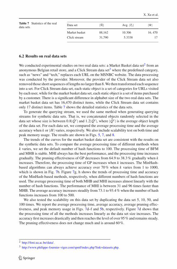
Table 7 Statistics of the realdata sets

Data set |R| Avg. |Ti | |�|Market basket 88,162 10.306 16, 470

Click stream 31,790 5.3338 17

6.2 Results on real data sets

We conducted experimental studies on two real data sets: a Market Basket data set2 from ananonymous Belgian retail store, and a Click Stream data set3 where the predefined category,such as “news” and “tech,” replaces each URL on the MSNBC website. The data processingwas conducted by the provider. Moreover, the provider of the Click Stream data set alsoremoved those short sequences of lengths no larger than 8. We then transformed each sequenceinto a set. For Click Stream data set, each static object is a set of categories for URLs visitedby each user, while for the market basket data set, each static object is a set of items purchasedby a customer. There is a significant difference in alphabet size of the two real data sets. Themarket basket data set has 16,470 distinct items, while the Click Stream data set containsonly 17 distinct items. Table 7 shows the detailed statistics of the data sets.

To generate the querying stream, we used the same method when generating queryingstreams for synthetic data sets. That is, we concatenated objects randomly selected in thedata set whose size is between 0.8|Q̄t | and 1.2|Q̄t |, where |Q̄t | is the average object lengthof the data set. For each data set, we compared the average processing time and the averageaccuracy when k or |H | varies, respectively. We also include scalability test on both time andpeak memory usage. The results are shown in Figs. 5, 7, and 8.

The trends of the curves for the market basket data set are consistent with the results onthe synthetic data sets. To compare the average processing time of different methods whenk varies, we set the default number of hash functions to 100. The processing time of BFMand MHB is stable. MHI always has the best performance, and the processing time increasesgradually. The pruning effectiveness of GP decreases from 64.9 to 38.3 % gradually when kincreases. Therefore, the processing time of GP increases when k increases. The MinHash-based algorithms can always achieve accuracy over 70 % when k varies from 1 to 1000,which is shown in Fig. 7b. Figure 7g, h shows the trends of processing time and accuracyof the MinHash-based methods, respectively, when different numbers of hash functions areused. The average processing time of both MHB and MHI increases almost linearly with thenumber of hash functions. The performance of MHI is between 31 and 96 times faster thanMHB. The average accuracy increases steadily from 73.1 to 93.4 % when the number of hashfunctions increases from 100 to 500.

We also tested the scalability on this data set by duplicating the data set 5, 10, 50, and100 times. We report the average processing time, average accuracy, average pruning effec-tiveness, and peak memory usage in Figs. 7d–f and 5b, respectively. Figure 7d shows thatthe processing time of all the methods increases linearly as the data set size increases. Theaccuracy first increases drastically and then reaches the level of over 95 % and remains steady.The pruning effectiveness does not change much and is around 60 %.

2 http://fimi.ua.ac.be/data/.3 http://www.philippe-fournier-viger.com/spmf/index.php?link=datasets.php.

123

http://fimi.ua.ac.be/data/

http://www.philippe-fournier-viger.com/spmf/index.php?link=datasets.php


BFM MHB GP MHI

1

10

100

1000

1 10 100 1000

Avg

. Pro

cess

ing

Tim

e (m

s)

k

Varying k

(a)

50

60

70

80

90

100

1 10 100 1000

Avg

. Accur

acy

(%)

k

Varying k

(b)

0

20

40

60

80

100

1 10 100 1000Avg

. Pru

ning

Eff

ectiv

enes

s (%

)

k

Varying k

(c)

1

10

100

1000

10000

1 5 10 50 100

Avg

. Pro

cess

ing

Tim

e (m

s)

Scale Factor


50

60

70

80

90

100

1 5 10 50 100

Avg

. Accur

acy

(%)

Scale Factor


0

20

40

60

80

100

1 5 10 50 100

Avg

. Pru

ning

Eff

ectiv

enes

s (%

)

Scale Factor


1

100

200300

100 200 300 400 500

Avg

. Pro

cess

ing

Tim

e(m

s)



50

60

70

80

90

100

100 200 300 400 500

Avg

. Accur

acy

(%)



(d)

(e) (f)

(g) (h)

Fig. 7 Results on market basket data set. aVary k (time), b vary k (accuracy), c vary k (pruning effectiveness),d vary |R| (time), e vary |R| (accuracy), f vary |R| (pruning effectiveness), g vary |H | (time), h vary |H |(accuracy)

123

X. Xu et al.

BFM MHB GP MHI

0.1

1

10

100

1 10 100 1000

Avg

. Pro

cess

ing

Tim

e (m

s)

k

Varying k

50

60

70

80

90

100

1 10 100 1000

Avg

. Accur

acy

(%)

k

Varying k

0

20

40

60

80

100

1 10 100 1000Avg

. Pru

ning

Eff

ectiv

enes

s (%

)

k

Varying k

1

10

100

1000

10000

1 10 100 1000

Avg

. Pro

cess

ing

Tim

e (m

s)

Scale Factor


50

60

70

80

90

100

1 10 100 1000

Avg

. Accur

acy

(%)

Scale Factor


50

60

70

80

90

100

1 10 100 1000

Avg

. Pru

ning

Eff

ectiv

enes

s (%

)

Scale Factor


1

20304050

20 40 60 80 100

Avg

.Pro

cess

ing

Tim

e(m

s)



50

60

70

80

90

100

20 40 60 80 100

Avg

.Accur

acy

(%)



(a) (b)

(c) (d)

(e) (f)

(g) (h)

Fig. 8 Results on click stream data set. a Vary k (time), b vary k (accuracy), c vary k (pruning effectiveness),d vary |R| (time), e vary |R| (accuracy), f vary |R| (pruning effectiveness), g vary |H | (time), h vary |H |(accuracy)

123


The peak memory usage is shown in Fig. 5b. The peak memory size used of all the methodsincreases almost linearly when the data set increases. Similar to the results in the scalabilitytest on the synthetic data sets, GP uses only a little more memory than BFM. Their trends aresimilar. The MinHash-based methods consume more space than BFM and GP. The reason isthe same as explained on the synthetic data sets in Sect. 6.1.1.

The results on the click stream data set are shown in Figs. 8 and 5c. Since the average lengthof the objects in this data set is only 5.33, the MinHash-based algorithms do not need manyhash functions in order to achieve high accuracy. As shown in Fig. 8h, the average accuracyis higher than 90 % when 40 or more hash functions are used. To test the performance when kvaries, we used 50 hash functions as the default. When k varies, MHI is still the best methodwith respect to average query answering time. The average accuracy drops gradually from 90to 67 %. As shown in Fig. 8c, the pruning effectiveness of GP decreases from 75.8 to 54.2 %,which is generally better than the results on the market basket data set.

We tested the scalability on the click stream data set by duplicating the data set 10, 100, and1000 times. Figures 8d–f and 5c show how the average processing time, average accuracy,average pruning effectiveness, and peak memory usage change with respect to different scaleof data set, respectively. The average processing time of all the methods increases almostlinearly when the data set size increases. MHI always achieves the lowest processing timeand outperforms the baselines by more than an order of magnitude. Moreover, it reports withreasonably high accuracy in the range of 81.6 and 90 % as shown in Fig. 8e. When the dataset size increases, the pruning effectiveness of GP increases steadily and is generally higherthan the results on the market basket data set.

The memory usage of BFM, GP, and MHB is very close and the corresponding curvesin Fig. 5c overlap with each other. Comparing to the other data sets, the memory usage ofMHB is much closer to BFM and GP because we use less number of hash functions. MHIstill consumes more memory due to the inverted indices data structure. However, its memoryusage is much closer to the other three methods comparing to the results on the other datasets. Recall that the size of our indexing structure depends on the number of hash functionsused and the alphabet size.

6.3 Summary

We conclude the following from our experiments. First, the pruning-based method is an exactmethod and the hashing-based method can achieve very good accuracy when a few hundredsof hash functions are used. The hashing-based method can lead to good accuracy and canachieve faster average querying time than the pruning-based method in most cases. However,when k increases, the accuracy drops and the running time increases greatly. The pruning-based method runs slower but maintains relatively stable running time with increasing k.For the hashing-based method, usually larger number of hash functions |H | provides betteraccuracy but also takes more running time. However, when the number of hash functionsexceeds 1,000, the increase in accuracy usually is very minor. As shown on synthetic dataset, when the average object length |Qt | becomes larger, the accuracy of the hashing-basedmethod drops greatly while the pruning effectiveness of the pruning-based method increasessignificantly, which implies that the pruning-based method is more feasible in this case. Ingeneral, both methods achieve better performance on data sets with larger lexicon size |�|.The sparser the data, the more significant the difference on similarity, and usually the betterruntime performance.

123

X. Xu et al.

7 Conclusions

In this paper, we studied the problem of continuous similarity search for evolving queries.To the best of our knowledge, it is the first research endeavor on this problem. We devisedtwo efficient methods with different framework. The pruning-based method uses pruningstrategies to reduce the cost of computing the exact similarity scores. The MinHash-basedmethod approximates the Jaccard similarity score based on MinHash technique and efficientlyupdates the estimated scores using indexing structures. The empirical results on syntheticand real data sets verify the effectiveness and efficiency of our methods.

As for future work, we plan to consider the following interesting directions.

– Enhance the pruning effectiveness For example, we may incorporate the evolving featureinto the pruning techniques used in static similarity join and search algorithms to furtherprune candidates.

– Improve the hashing-based method for other similarity measures We may extend ourhashing-based framework to other similarity and distance measures that can be approxi-mated by an LSH scheme used in MinHash.

– Similarity search over multiple evolving streams Given a static object and multiple datastreams with a fixed sliding window size, we may want to continuously find the top-k datastreams whose last n items are most similar to the static object. The techniques proposedin this paper can be further extended for the problem.

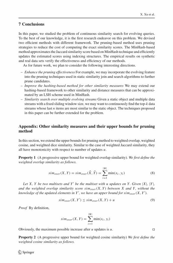
Appendix: Other similarity measures and their upper bounds for pruningmethod

In this section, we extend the upper bounds for pruning method to weighted overlap, weightedcosine, and weighted dice similarity. Similar to the case of weighted Jaccard similarity, theyall have monotonicity with respect to number of updates u.

Property 1 (A progressive upper bound for weighted overlap similarity). We first define theweighted overlap similarity as follows.

simover (X, Y ) = simover ( �X , �Y ) =|�|∑

i=1

min(xi , yi ) (8)

Let X, Y be two multisets and Y ′ be the multiset with u updates on Y . Given |X |, |Y |,and the weighted overlap similarity score simover (X, Y ) between X and Y , without theknowledge of the updated elements in Y ′, we have an upper bound for simover (X, Y ′).

simover (X, Y ′) ≤ simover (X, Y ) + u (9)

Proof By definition,

simover (X, Y ) =|�|∑

i=1

min(xi , yi )

Obviously, the maximum possible increase after u updates is u. ��Property 2 (A progressive upper bound for weighted cosine similarity) We first define theweighted cosine similarity as follows.

123


simcos(X, Y ) = simcos( �X , �Y ) =∑|�|

i=1 min(xi , yi )√|X ||Y | (10)

Let X, Y be two multisets and Y ′ be the multiset with u updates on Y . Given |X |, |Y |, andthe weighted cosine similarity score simcos(X, Y ) between X and Y , without the knowledgeof the updated elements in Y ′, we have an upper bound for simcos(X, Y ′).

simcos(X, Y ′) ≤ simcos(X, Y ) + u√|X ||Y | (11)

Proof In our scenario, |Y | = |Y ′|. Thus,√|X ||Y | = √|X ||Y ′|. By Property 1, we have

simcos(X, Y ′) ≤∑|�|

i=1 min(xi , yi ) + u√|X ||Y ′| = simcos(X, Y ) + u√|X ||Y |��

Property 3 (A progressive upper bound for weighted dice similarity) We first define theweighted dice similarity as follows.

simdice(X, Y ) = simdice( �X , �Y ) = 2∑|�|

i=1 min(xi , yi )

|X | + |Y | (12)

Let X, Y be two multisets and Y ′ be the multiset with u updates on Y . Given |X |, |Y |, andthe weighted dice similarity score simdice(X, Y ) between X and Y , without the knowledgeof the updated elements in Y ′, we have an upper bound for simdice(X, Y ′).

simdice(X, Y ′) ≤ simdice(X, Y ) + 2u

|X | + |Y | (13)

Proof In our scenario, |Y | = |Y ′|. Thus, |X | + |Y | = |X | + |Y ′|. By Property 1, we have

simdice(X, Y ′) ≤ 2∑|�|

i=1 min(xi , yi ) + 2u

|X | + |Y ′| = simdice(X, Y ) + 2u

|X | + |Y |��

References

1. Andoni A, Indyk P (2006) Near-optimal hashing algorithms for approximate nearest neighbor in highdimensions. In: Proceedings of the 47th annual IEEE symposium on foundations of computer science,FOCS ’06, Washington, DC, USA. IEEE Computer Society, pp 459–468

2. Artin E (2011) Geometric algebra. Wiley, Hoboken3. Bayardo RJ, Ma Y, Srikant R (2007) Scaling up all pairs similarity search. In: Proceedings of the 16th

international conference on World Wide Web, WWW ’07, New York, NY, USA. ACM, pp 131–1404. Böhm C, Ooi BC, Plant C, Yan Y (2007) Efficiently processing continuous k-nn queries on data streams.

In: Proceedings of the international conference on data engineering, ICDE ’07, Washington, DC, USA.IEEE Computer Society, pp 156–165

5. Broder A (1997) On the resemblance and containment of documents. In: Proceedings of the compressionand complexity of sequences 1997, SEQUENCES ’97, Washington, DC, USA. IEEE Computer Society,pp 21–29

6. Broder AZ, Charikar M, Frieze AM, Mitzenmacher M (2000) Min-wise independent permutations. JComput Syst Sci 60(3):630–659

7. Charikar MS (2002) Similarity estimation techniques from rounding algorithms. In: Proceedings of thethirty-fourth annual ACM symposium on theory of computing, STOC ’02, New York, NY, USA. ACM,pp 380–388

123

X. Xu et al.

8. Chaudhuri S, Ganti V, Kaushik R (2006) A primitive operator for similarity joins in data cleaning. In:Proceedings of the 22nd international conference on data engineering, ICDE ’06, Washington, DC, USA.IEEE Computer Society, pp 5–15

9. Cohen WW (1998) Integration of heterogeneous databases without common domains using queries basedon textual similarity. In: Proceedings of the 1998 ACM SIGMOD international conference on managementof data, SIGMOD ’98, New York, NY, USA. ACM, pp 201–212

10. Cost S, Salzberg S (1993) A weighted nearest neighbor algorithm for learning with symbolic features.Mach Learn 10(1):57–78

11. Datar M, Muthukrishnan S (2002) Estimating rarity and similarity over data stream windows. In: Pro-ceedings of the 10th annual European symposium on algorithms, ESA ’02. Springer, London, pp 323–334

12. Devroye L, Wagner TJ (1982) 8 nearest neighbor methods in discrimination. Handbook of statistics2:193–197

13. Faloutsos C, Barber R, Flickner M, Hafner J, Niblack W, Petkovic D, Equitz W (1994) Efficient andeffective querying by image content. J Intell Inf Syst 3(3–4):231–262

14. Faloutsos C, Oard DW (1995) A survey of information retrieval and filtering methods. University ofMaryland at College Park, College Park, MD, USA. Univ. of Maryland Institute for Advanced ComputerStudies Report

15. Flickner M, Sawhney H, Niblack W, Ashley J, Huang Q, Dom B, Gorkani M, Hafner J, Lee D, PetkovicD, Steele D, Yanker P (1995) Query by image and video content: the qbic system. Computer 28(9):23–32

16. Gersho A, Gray RM (1991) Vector quantization and signal compression. Kluwer Academic Publishers,Norwell

17. Gionis A, Indyk P, Motwani R (1999) Similarity search in high dimensions via hashing. In: Proceedings ofthe 25th international conference on very large data bases, VLDB ’99, San Francisco, CA, USA. MorganKaufmann Publishers Inc., pp 518–529

18. Hastie T, Tibshirani R (1995) Discriminant adaptive nearest neighbor classification. In: Proceedings ofthe first international conference on knowledge discovery and data mining, KDD ’95, Palo Alto, CA,USA. AAAI Press, pp 142–149

19. Henzinger M (2006) Finding near-duplicate web pages: a large-scale evaluation of algorithms. In: Proceed-ings of the 29th annual international ACM SIGIR conference on research and development in informationretrieval, SIGIR ’06, New York, NY, USA. ACM, pp 284–291

20. Indyk P (2001) A small approximately min-wise independent family of hash functions. J Algorithms38(1):84–90

21. Indyk P, Motwani R (1998) Approximate nearest neighbors: towards removing the curse of dimensionality.In: Proceedings of the thirtieth annual ACM symposium on theory of computing, STOC ’98, New York,NY, USA. ACM, pp 604–613

22. Koivune V, Kassam S (1995) Nearest neighbor filters for multivariate data. In: IEEE workshop on nonlinearsignal and image processing, Washington, DC, USA. IEEE Computer Society, pp 734–737

23. Kollios G, Tsotras VJ (2002) Hashing methods for temporal data. IEEE Trans Knowl Data Eng 14(4):902–919

24. Kontaki M, Papadopoulos AN (2004) Efficient similarity search in streaming time sequences. In: Pro-ceedings of the 16th international conference on scientific and statistical database management, SSDBM’04, Washington, DC, USA. IEEE Computer Society, pp 63–72

25. Koudas N, Ooi BC, Tan K-L, Zhang R (2004) Approximate nn queries on streams with guaranteederror/performance bounds. In: Proceedings of the thirtieth international conference on very large databases, VLDB ’04. VLDB Endowment, pp 804–815

26. Lian X, Chen L, Wang B (2007) Approximate similarity search over multiple stream time series. In:Proceedings of the 12th international conference on database systems for advanced applications, DAS-FAA’07. Springer, Berlin, pp 962–968

27. Mouratidis K, Bakiras S, Papadias D (2006) Continuous monitoring of top-k queries over sliding windows.In: Proceedings of the 2006 ACM SIGMOD international conference on management of data, SIGMOD’06, New York, NY, USA. ACM, pp 635–646

28. Mouratidis K, Papadias D (2007) Continuous nearest neighbor queries over sliding windows. IEEE TransKnowl Data Eng 19(6):789–803

29. Mouratidis K, Papadias D, Bakiras S, Tao Y (2005) A threshold-based algorithm for continuous monitoringof k nearest neighbors. IEEE Trans Knowl Data Eng 17(11):1451–1464

30. Pan S, Zhu X (2012) Continuous top-k query for graph streams. In Proceedings of the 21st ACM interna-tional conference on information and knowledge management. CIKM ’12, New York, NY, USA. ACM,pp 2659–2662

31. Pentland A, Picard RW, Sclaroff S (1994) Photobook: content-based manipulation of image databases.In: Storage and retrieval for image and video databases, Bellingham, WA, USA. SPIE, pp 34–47

123


32. Rao W, Chen L, Chen S, Tarkoma S (2014) Evaluating continuous top-k queries over document streams.World Wide Web 17(1):59–83

33. Salton G, McGill MJ (1986) Introduction to modern information retrieval. McGraw-Hill Inc., New York34. Sarawagi S, Kirpal A (2004) Efficient set joins on similarity predicates. In: Proceedings of the 2004 ACM

SIGMOD international conference on management of data, SIGMOD ’04, New York, NY, USA. ACM,pp 743–754

35. Smeulders A, Jain R (eds) (1998) Image databases and multimedia search. World Scientific PublishingCo., Inc., River Edge

36. Sun Y, Han J, Yan X, Yu PS, Wu T (2011) Pathsim: meta path-based top-k similarity search in heteroge-neous information networks. Proc VLDB Endow 4(11):992–1003

37. Winkler WE (1999) The state of record linkage and current research problems. Statistical ResearchDivision, US Census Bureau, Suitland

38. Xiao C, Wang W, Lin X, Yu JX (2008) Efficient similarity joins for near duplicate detection. In: Proceed-ings of the 17th international conference on World Wide Web, WWW ’08, New York, NY, USA. ACM,pp 131–140

Xiaoning Xu received her Master’s degree in computing science fromSimon Fraser University, Canada in 2014, supervised by Prof. Jian Pei.Previously, she was in the SFU-ZJU computing science dual degreeprogram. She received a B.Sc. degree from Simon Fraser University,Canada, and a B.Eng. degree from Zhejiang University, China, both in2012. Her research interests focus on similarity search and data streamprocessing. She is currently a software engineer at Fortinet Inc., work-ing on data analytics and threat detection in network log data.

Chuancong Gao is a Ph.D. student in computing science in SimonFraser University, Canada, since 2013, supervised by Prof. Jian Pei.Previously he received a master degree from Tsinghua University,China, in 2010 and a bachelor degree from Shandong University,China, in 2007, both in computer science and in engineering. His cur-rent research interests are data cleaning and data integration.

123

X. Xu et al.

Jian Pei is the Canada Research Chair in Big Data Science and aprofessor at the School of Computing Science and the Department ofStatistics and Actuarial Science at Simon Fraser University, Canada.He received a Ph.D. degree at the same school in 2002 under Dr. JiaweiHan’s supervision. His research interests are to develop effective andefficient data analysis techniques for novel data intensive applications.He has published prolifically and is one of the top cited authors in datamining. He received a series of prestigious awards. He is also active inproviding consulting service to industry and transferring the researchoutcome in his group to industry and applications. He is an editor ofseveral esteemed journals in his areas and a passionate organizer of thepremier academic conferences and initiatives defining the frontiers ofthe areas. He is an IEEE fellow.

Ke Wang received Ph.D. from Georgia Institute of Technology. Heis currently a professor at the School of Computing Science, SimonFraser University. His research interests include database technology,data mining, and knowledge discovery, with emphasis on massive datasets, graph and network data, and data privacy. Ke Wang has pub-lished more than 100 research papers in database, information retrieval,and data mining conferences. He is currently an associate editor of theACM TKDD journal.

Abdullah Al-Barakati was the head of Information Systems Depart-ment at King Abdulaziz University (KAU), Jeddah, Saudi Arabia, sincein the period 2014–2015. He is also a faculty member and a lecturerin the Faculty of Computing and Information Technology since theyear 2013. Dr. Al-Barakati’s academic interests range from teachingand academic research to modern theories in applied informatics. Hisresearch interests revolve on the area of Big Data ranging from mod-ern practices in Big Data to advanced concepts and special issues inBig Data mining (pattern extraction, visualization, and analysis). Lan-guage Processing (LP) and Machine Learning (ML) also fall withinhis research interests as he has developed a passion for text analy-sis and manipulation. Furthermore, web applications especially thedynamics of Social Media and web 2.0 are important elements of Dr.Al-Barakati’s research interests as he believes that they form the cor-nerstones of many astonishing innovations now and in the future.

123

Continuous similarity search for evolving queriesjpei/publications... · · 2016-06-06Continuous...

Documents

Transcript of Continuous similarity search for evolving queriesjpei/publications... · · 2016-06-06Continuous...