HAL Id: hal-01188367https://hal.inria.fr/hal-01188367

Submitted on 29 Aug 2015

HAL is a multi-disciplinary open accessarchive for the deposit and dissemination of sci-entific research documents, whether they are pub-lished or not. The documents may come fromteaching and research institutions in France orabroad, or from public or private research centers.

L’archive ouverte pluridisciplinaire HAL, estdestinée au dépôt et à la diffusion de documentsscientifiques de niveau recherche, publiés ou non,émanant des établissements d’enseignement et derecherche français ou étrangers, des laboratoirespublics ou privés.

Continuous and Discrete State Estimation for SwitchedLPV Systems using Parameter Identification

Hector Ríos, D Mincarelli, Denis Efimov, Wilfrid Perruquetti, J Davila

To cite this version:Hector Ríos, D Mincarelli, Denis Efimov, Wilfrid Perruquetti, J Davila. Continuous and DiscreteState Estimation for Switched LPV Systems using Parameter Identification. Automatica, Elsevier,2015, 62, pp.1-8. 10.1016/j.automatica.2015.09.016. hal-01188367

Continuous and Discrete State Estimation for Switched LPV

Systems using Parameter Identification ?

H. Rıos a, D. Mincarelli a, D. Efimov a,b, W. Perruquetti a and J. Davila c

aNon-A team @ Inria, Parc Scientifique de la Haute Borne, 40 avenue Halley, 59650 Villeneuve d’Ascq, France and CRIStAL(UMR-CNRS 9189), Ecole Centrale de Lille, BP 48, Cite Scientifique, 59651 Villeneuve-d’Ascq, France (e-mails:

hector.rios barajas@inria.fr, diego.mincarelli@inria.fr, denis.efimov@inria.fr, wilfrid.perruquetti@inria.fr)

bDepartment of Control Systems and Informatics, Saint Petersburg State University of Information Technologies Mechanicsand Optics (ITMO), 49 Kronverkskiy av., 197101 Saint Petersburg, Russia.

cNational Polytechnic Institute, Section of Graduate Studies and Research, ESIME-UPT, C.P. 07340, Mexico D.F., (e-mail:jadavila@ipn.mx)

Abstract

In this paper the problem of discrete and continuous state estimation for a class of uncertain switched LPV systems isaddressed. Parameter identification techniques are applied to realize an approximate identification of the scheduled parametersof a switched LPV system with certain uncertainties and/or disturbances. A discrete state estimation is achieved using theparameter identification. A Luenberger-like hybrid observer, based on discrete state information and LMIs approach, is usedfor the continuous state estimation. The simplicity of the proposed method is one of the main advantages of this paper. Thefeasibility of the proposed method is illustrated by simulations.

Key words: Switched systems; LPV Systems; State estimation.

1 INTRODUCTION

In the last two decades, the linear parameter varying(LPV) systems have received a lot of the attention fromthe control area [17]. Such a kind of systems was intro-duced by [25] in order to establish a difference betweenlinear time invariant and linear time varying systems.LPV systems represent a class of linear systems whosestate/input matrices depend on a set of time varying pa-rameters which can be measured in real time. For pro-cesses with mild nonlinearities or dependence on exter-nal variables, it has been shown that LPV equivalentrepresentation offers an attractive modeling framework.The practical use of LPV systems is stimulated by thefact that control design for LPV systems is well known(see, e.g. gain scheduling [23], µ−synthesis [30], and lin-ear matrix inequalities (LMIs) based optimal control[24]) since these systems allow us to apply linear designtools to complex nonlinear models. Closely related tothe LPV systems, the switched systems are described bythe interaction of continuous and discrete state dynam-

? This work has been partially presented at 2014 AmericanControl Conference [22]. Corresponding author H. Rıos.

ics. This kind of systems has been widely studied dur-ing the last decades since they can be used to describe awide range of physical and engineering systems (see, e.g.[11]). However, for an LPV system with a large parame-ter variation region, a single controller may not exist orthe numerical routines for solution calculation may failto converge. If such a controller exist, the performancemay be sacrificed, in some parameter regions, trying todesign a single controller that is able to act over thewhole region. A reasonable approach to avoid this kindof problems is to design several LPV systems and con-trollers, each of them suitable for a specific parametersubregion, and changing among them to fulfill certainpossible performance. Then, such a model belongs to anew kind of systems, switched LPV systems. In this con-text, the switched LPV systems have attracted the at-tention of many researchers and many results have beenachieved about multi-Lyapunov functions for analysis,controller design, and modelling for such systems (see,e.g. [6], [15], [28] where the asynchronous switching esti-mation problem has been proposed for the first time andthe used multiple Lyapunov-like functions approach isallowed to be locally increasable upon which the asyn-chronous switched filter/observer can be designed, and

Preprint submitted to Automatica 10 August 2015

[29]). On the control design, the switched LPV controltechniques allow us to use different controllers for eachparameter subregion and switch among them accordingto the evolution of the discrete state. This technique isalso beneficial in order to improve the control perfor-mance and enhance the design flexibility (see, e.g. [7]and [16]). Nevertheless, most of the switched LPV con-trol approaches are designed taking into account thatthe discrete state (switching law) is independent of thesystem parameters, i.e. it is known. For this reason,the knowledge of the discrete state becomes crucial. Forswitched systems, the discrete state estimation problemhas been dealt with in many works. Usually, an observerscheme is designed to estimate the discrete state andthen, based on this information, the continuous one canbe reconstructed (see, e.g. based on sliding mode ob-server approach [1], [4], and on algebraic approach [3]).The reverse procedure can also be applied, i.e. discretestate estimation based on the continuous state informa-tion, as it is described by [19] and [21], based on slidingmode observers. In [27] necessary and sufficient condi-tions for a linear switched systems to be invertible areproposed, i.e. condition for recovering the switching sig-nal (discrete state) and the input uniquely. However, tothe best of our knowledge, the discrete and continuousstate estimation problem in switched LPV systems hasnot been fully tackled yet. Motivated in the previousexplanations and by some recent practical applications(active magnetic bearing systems [15], missile autopilotsystems [12], F-16 aircraft system [16], wind turbine [10],and air path system of diesel engine [13]), in this paperthe problem of discrete and continuous state estimationfor switched LPV systems is addressed. In such systemsthe discrete state is unknown, and the system behaviorcan be represented by the interaction of LPV subsystemswith unmeasured vector of time-varying scheduling pa-rameters (continuous dynamics) and some commutationoperating modes (discrete dynamics).

Main Contribution: A solution to the problem ofdiscrete and continuous state estimation for a class ofswitched LPV systems under uncertainties is proposedby means of parameter identification techniques and aLuenberger-like hybrid observer, respectively. Takinginto account that the time-varying vector of schedulingparameters is unmeasurable, the basic idea to fulfill theaforementioned goal is as follows: 1) The discrete stateestimation is achieved by means of the identification ofthe system parameters (assuming that the parameterslie on different known regions of the parameter space).2) The continuous state is estimated by means of ahybrid observer that uses the discrete state information.

For the parameter identification, a simple Least SquareMethod is proposed. Due to one of the objectives is toobtain a practical solution, a simple algorithm is ap-plied. However, the simplicity of the proposed methodis one of the main advantages of this work. For the hy-brid observer, a Luenberger-like approach is used based

on LMIs. Simulation results illustrate the feasibility ofthe proposed methods.

Structure of the Paper: Section 2 deals with the prob-lem statement and some preliminaries. In section 3 theparameter identification method is described and the al-gorithm to estimate the discrete state is given. Section 4shows how to design an observer to estimate the continu-ous state. The simulation results are shown in section 5.Finally, some concluding remarks are given in section 6.

Notation: For a vector x ∈ Rn, the symbol ‖·‖∞ de-notes the infinity norm, i.e. ‖x‖∞ = max (|x1| , ..., |xn|).The Euclidean norm is denoted by ‖·‖2. Let R+ =t ∈ R : t ≥ 0. For a locally essentially bounded inputu : R+ → R the symbol ‖u‖[t0,t1] denotes its L∞ norm,

i.e. ‖u‖[t0,t1] = ess supt∈[t0,t1] ‖u(t)‖2, if t1 = +∞ then

the symbol ‖u‖ will be used. Denote by L∞ the set ofall inputs u that satisfy ‖u‖ < +∞. The convolutionoperation ∗, on two functions f and g, is defined as

f(t) ∗ g(t) =∫ t0f(τ)g(t − τ)dτ . The 1-norm for a func-

tion f : [a, b] → R is defined by ‖f‖1 =∫ ba|f(t)| dt. For

a matrix Q ∈ Rm×n, the induced matrix norm is definedby ‖Q‖m =

√λmax(QTQ), where λmax is the maximum

eigenvalue of QTQ.

2 PROBLEM STATEMENT

In this work the following switched LPV system is con-sidered 1 :

y(n)(t) = −n−1∑i=0

ai (σ(t), ρ(t)) y(i)(t)

+

m∑j=0

bj (σ(t), ρ(t))u(j)(t) + ε(t), (1)

where y, u ∈ R, are the output and the input, re-spectively, generated by the switched LPV system. Theterm ε(t) ∈ L∞ represents uncertainties, disturbancesand/or high frequency perturbations (possible effects ofthe noise in the input/output reflected in y(n)(t)) in thesystem, and it is considered that the following assump-tion holds:

Assumption 1 The uncertain term ε(t) is essentiallybounded, i.e. ‖ε‖ ≤ ε+, where ε+ is a known positiveconstant.

The so-called “discrete state” σ(t) : R+ → Q =1, ..., q determines the current system dynam-ics among the possible q “operating modes”. The

1 In the literature there exist works dealing with the trans-formation of time varying systems to canonical forms, as in(1), see, e.g. [20] and [26].

2

unknown scheduling parameter is represented byρ(t) : R+ → Θ ⊆ R and it belongs to L∞. The parame-ters a0 : Q×Θ → Iσa0 ⊆ R, a1 : Q×Θ → Iσa1 ⊆ R, . . . ,an−1 : Q×Θ→ Iσan−1

⊆ R, and b0 : Q×Θ→ Iσb0 ⊆ R,b1 : Q × Θ → Iσb1 ⊆ R, . . . , bm : Q × Θ → Iσbm ⊆ Rare unknown, where Iσ(·) are given compact sets. The

parameters ai(σ, ρ(t))n−1i=0 and bj(σ, ρ(t))mj=0 evolve

in a compact set Ωσ = Iσa0× . . .× Iσan−1× Iσb0× . . .× I

σbm

,which changes when σ takes different values in Q. Inthe following, it is assumed that time-varying vectorof scheduling parameters is not accessible for measure-ments and only the domains Ωσ are known for everyvalue of σ in Q. The aim of this paper is to estimate thediscrete state σ(t) by the measurements of the outputy(t) and input u(t). Then, estimate the continuous state,i.e. y(k) for k = 0, 1, ..., n− 1.

2.1 Preliminaries

Define the parameter vector for the discrete state σ as

θ(σ, ρ(t)) = [a0(·), . . . , an−1(·), b0(·), . . . , bm(·)]T ∈ Ωσ.Some definitions for distinguishability and observabilityof the discrete state are introduced in the following.

Definition 1 Distinguishability of the system. Thesystem (1) is called distinguishable, if for every pair (i, j),

the identity y (t, θ(i, ρ(t))) = y(t, θ(j, ρ(t))), ∀t ∈ [t1, t2],

implies that i = j, and θ, θ ∈ Ωi, for a given input u andi, j ∈ Q, for ∀t ∈ [t1, t2].

Definition 2 Observability of the discrete state.The discrete state σ(t) is observable if the system (1) isdistinguishable, and θ(σ(t), ρ(t)) 6∈

(Ω1 ∩ · · · ∩ Ωq

)dur-

ing any time interval (see Fig. 1).

Fig. 1 depicts the discrete state observability definition.Note that θ(σ(t), ρ(t)) may cross the set

(Ω1 ∩ · · · ∩ Ωq

)for an instant of time, e.g. due to the switchings, butwhile θ(σ(t), ρ(t)) does not remain in

(Ω1 ∩ · · · ∩ Ωq

)during any time interval, the discrete state will be ob-servable (see Fig. 1 left top case). On the contrary, ifθ(σ(t), ρ(t)) belongs to

(Ω1 ∩ · · · ∩ Ωq

)during a time in-

terval (as in Fig. 1 right top case), the discrete state willnot be observable over this time interval.

2.2 Description of the Proposed Solution

The system (1) can be written in the regressor form as

y(n)(t) = θ (σ(t), ρ(t))φ(t) + ε(t), (2)

where θ (·) ∈ R1×r is the unknown varying parame-

ter vector, and φ(t) = [ y(t), · · · , y(n−1)(t), u(t), · · · ,u(m)(t)]T ∈ Rr×1 is the regressor vector, where r =n+m+1. It is considered that the following assumptionholds.

Ia0j

Ib0i

Ib0j

𝛀𝒋

𝛀𝐢 Ia0i 𝒕

𝒂𝟎

𝒃𝟎

𝛀𝐢 ∩ 𝛀𝐣

𝛉(𝛔 𝐭 , 𝛒(𝐭))

Ia0j

Ib0i

Ib0j

𝛀𝒋

𝛀𝐢 Ia0i 𝒕

𝒂𝟎

𝒃𝟎

𝛀𝐢 ∩ 𝛀𝐣

𝛉(𝛔 𝐭 , 𝛒(𝐭))

Ia0j

Ib0i

Ib0j

𝛀𝒋

𝛀𝐢 Ia0i 𝒕

𝒂𝟎

𝒃𝟎

𝛉(𝛔 𝐭 , 𝛒(𝐭))

Fig. 1. Observability of the discrete state. From thegeometric point of view, it is easy to see that the discretestate is observable for every θ, if Ωi ∩ Ωj = ∅ (the triv-ial case - bottom graph). The first two graphs correspond tothe case Ωi ∩ Ωj 6= ∅. The top one illustrates an observ-able discrete state case with non-empty intersections, i.e.θ(σ(t), ρ(t)) 6∈

(Ωi ∩ Ωj

)during any time interval, and the

middle one depicts an unobservable discrete state case.

Assumption 2 The time derivative of the parametervector is essentially bounded, i.e. ‖θ (σ(t), ρ(t)) ‖2 ≤ εθ,for almost all t ≥ 0, with a known positive constant εθ.

The discrete state estimation problem can be solved ifit is possible to identify the unknown parameter vectorθ (σ(t), ρ(t)) under the assumption that the domains Ωσ

for all σ ∈ Q are known and the conditions of Definitions1 and 2 are satisfied for all t ≥ 0.

Remark 1 Note that the main objective is to realize agood discrete state estimation and to do that it is notneeded to identify the parameters exactly. It is only nec-essary to provide an approximate estimation with a suffi-ciently small error that allows to distinguish between thediscrete states (see an example in Fig. 2). However, alarge error in the parameter identification could yield aconsiderable error in the continuous state estimation.

3 DISCRETE STATE ESTIMATION

In the literature there exist many methods to identifyconstant and varying parameters, and the most popu-lar ones belong to the group of least squares (LS) meth-ods (e.g., non-recursive method of LS, recursive meth-ods of LS, method of weighted LS, exponential forget-ting with constant forgetting factor, exponential forget-ting with variable forgetting factor, etc.). There exist

3

𝒕

𝒂𝟎

𝒃𝟎

𝛀𝒋 𝜹 𝛀𝒊 𝜹

𝛀𝐢

𝛀𝒋

𝛀𝐢 ∩ 𝛀𝐣 = ∅

𝛀𝒊 ∩ 𝛀𝐣 ≠ ∅ 𝜹 𝜹

𝛉 𝑳𝑺(𝛔 𝐭 , 𝛒(𝐭))

Fig. 2. Distinguishable sets Ωσ(t) with error. In the graphthe maximum parameter identification error is represented

by the variable δ and the parameter estimation by θLS, sothe estimation process will allow us to identify the set ofparameters with a bounded estimation error of order δ (sets

Ωiδ and Ωjδ), that is represented by the volume enclosed by

dotted line. Note that Ωi∩Ωj = ∅ while Ωiδ∩Ωjδ 6= ∅. However,

since θLS(σ(t), ρ(t)) 6∈ Ωiδ ∩ Ωjδ it is possible to estimate thediscrete state.

also many modifications of the LS methods (e.g., methodof generalized LS, method of extended LS, method ofbias correction, instrumental variables method, etc.),and bayesian method, maximum likelihood methods, ex-tended Kalman filter, modulating functions methods,subspace methods, etc. (see, e.g., [8] and [14]).

Note that to solve the formulated problem in this paper,it is possible to use any method that allows us to iden-tify the parameters with such a sufficiently small errorthat it is possible to distinguish the discrete state σ(t).It is necessary to mention that the objective is not to re-alize a good parameter identification for θ (·) but a goodestimation of σ(t). In the following, the used parameteridentification method is described.

3.1 Description of the Parameter Identification

Consider system (2) and apply the mean value theoremto each entry of θ (σ(t), ρ(t)). Then, (2) can be rewritten,for all t ∈ [t0, t0 + T ], as:

y(n)(t) =[θ (t0) + (t− t0)θ (c(t))

]φ(t) + ε(t), (3)

where θ (c(t)) = [ a0 (c0(t)) , a1 (c1(t)) , . . . , bm (cr(t)) ],

ci(t)ri=1 ∈ (t0, t0 + T ) represent time varying val-ues for each component of θ (σ(t), ρ(t)), θ (t0) =θ (σ(t0), ρ(t0)), and T is a positive constant that de-fines a time window in which it is expected that theparameter identification is carried out. Note that if thederivatives of the output y(t) and the input u(t) aredirectly measurable, these values can be entered di-rectly into the regressor vector φ(t) and therefore theclassical LS method can be applied directly to estimate

θ (t0) on [t0, t0 + T ]. However, the derivatives are notmeasurable, the parameters are time variant, and thereexist some uncertainties, disturbances or/and noise.Therefore, some considerations have to be made.

Firstly, in order to avoid the direct calculation of thederivatives of the output and input, the state variablefilter approach is used [8]. The main idea is to filter theoutput signal y(t) and input signal u(t) with the samestable Butterworth low-pass filter 2 that has the follow-ing structure in the Laplace domain:

F (s) =1

1 + λ1s+ · · ·+ λpsp, (4)

where p = max(n,m + 1), and the design of the filterparameters λk is free (stable filter). For example, one canset the design parameters so that F (s) has an arbitrarycut-off frequency ωc, and the form:

F (s) =1∏

j

(1 + αj

sωc

+ βjs2

ω2c

) ,with the coefficients being:

• Even p: αjp/2j=1 =

2 cos (2j−1)π2p

p/2j=1

,βjp/2j=1

= 1.

• Odd p: α1 = 1, αj(p+1)/2j=2 =

2 cos (j−1)π

p

(p+1)/2

j=2,

β1 = 0,βj(p+1)/2

j=2= 1.

After filtering, system (3), for all t ∈ [t0, t0 + T ], be-comes:

Y (t) = θ (t0) Ψ(t) + Θ(t) + Ξ(t), (5)

where Y (t) = f(t) ∗ y(n)(t), Ψ(t) = f(t) ∗ φ(t), Θ(t) =

f(t) ∗ ((t − t0)θ (σ (ci(t)) , ρ (ci(t)))φ(t)), and Ξ(t) =f(t)∗ε(t), where f(t) is the impulse response of the filter(4). If it is assumed that the uncertain terms Θ(t) andΞ(t), are equal to zero, then, post-multiplying by ΨT (t)and integrating, it is obtained∫ t0+T

t0

Y (τ)ΨT (τ)dτ = θ (t0)

∫ t0+T

t0

Ψ(τ)ΨT (τ)dτ,

where T is a positive constant that defines the time win-dow of identification. Thus, the classical LS Method canbe applied to estimate the term θ (t0), i.e.

θLS(t0) =

∫ t0+T

t0

Y (τ)ΨT (τ)dτΥ−1, (6)

2 One can choose a Butterworth low-pass filter or any othertype of low-pass filter, e.g. Bessel, Chebyshev, etc. (see, e.g.[5]).

4

with Υ =∫ t0+Tt0

Ψ(τ)ΨT (τ)dτ . In order to implement

(6) it is necessary to construct the new regressor vectorΨ(t) and the term Y (t), with this aim, the state variablefilter approach is used.

3.1.1 State Variable Filter Design.

The principle of state variable filters is to use a low-passfilter that damps out the higher frequency noise andtransform it into a state space representation, such thatthe states are the derivatives of the filter output, i.e. thefiltered signal. They are designed to suppress any noiseabove the cut-off frequency.

Consider that the regressor vector has the followingstructure

Ψ(t) =[yf0(t), ... , yfn−1

(t), uf0(t), ... , ufm(t)]T.

The elements of the vector Ψ(t) can be easily obtained asthe state variables of the following state space systems,which represent the controllable canonical form of thefilter (4), i.e.

yF (t) = AyF (t) + by(t), (7)

uF (t) = AuF (t) + bu(t), (8)

where yF (t) = [ yf0(t), ... , yfp−1(t) ]T ∈ Rp and

uF (t) = [ uf0(t), ... , ufp−1(t) ]T ∈ Rp and

A =

0 1 0 · · · 0

0 0 1 · · · 0

......

.... . .

...

0 0 0 · · · 1

− 1λp− λ1λp− λ2λp· · · −λp−1

λp

, b =

0

0

...

0

1λp

.

Note that, since yfp−1(t) = yfp(t), yfp(t) can be con-

structed as follows:

yfp(t) =

[− 1

λp,−λ1

λp, ...,−λp−1

λp

]yF (t) +

1

λpy(t). (9)

For the linear time-invariant systems (7), in the sameway for (8); assuming that the filter initial conditions areequal to zero, it is possible to express the n and m + 1transfer functions, respectively, as follows:

Yfi(s) =si

1 + λ1s+ · · ·+ λpspY (s), i = 0, ..., n− 1.

Ufj (s) =sj

1 + λ1s+ · · ·+ λpspU(s), j = 0, ...,m.

In order to calculate the filter transient time ξ is nec-essary to consider the Laplace transformation existence

of the corresponding input filter, i.e. the convergence of∫∞0|y(t)| e−αtdt, for α > 0. It is well-known that this

integral converges if |y(t)| < Γe%t, ∀t > 0, some Γ > 0,and α > %; in the same way for u(t). In this sense, if thecorresponding filter input satisfies such a condition thenthe following procedure is proposed to calculate the fil-ter transient time:

1. Design the parameters for filter (4).2. Express the filter inputs, i.e. y(t) and u(t), in the

Laplace domain.3. Obtain the corresponding transfer functions, i.e.Yf0(s), . . . , Yfn−1(s) and Uf0(s), . . . , Ufm(s) 3 .

4. Obtain the partial fraction expansion for each transferfunction.

5. Apply the inverse Laplace transformation for eachtransfer function.

6. Identify the transient part for each solution yf0(t), . . . ,yfn−1

(t) and uf0(t), . . . , ufm(t), respectively.7. Calculate the transient time 4 for each solution, i.e.ξy0 , . . . , ξyn−1

and ξu0, . . . , ξum , assuming a tolerance

band.8. Define ξ as the slowest transient time.

Otherwise:

1. Design the parameters for filter (4).2. Simulate the state space systems (7) and (8) with their

corresponding inputs.3. Calculate by simulation the transient time for each so-

lution, i.e. ξy0 , . . . , ξyn−1and ξu0

, . . . , ξum , assuminga tolerance band.

4. Define ξ as the slowest transient time.

Note that it is possible to modify the corresponding tran-sient times by adjusting the filter parameters (analyti-cally or by simulation). However, there will be a trade-off between the desired transient time and the corre-sponding cut-off frequency. It is also worth highlightingtwo points of the first procedure: 1) this procedure canbe applied for any filter input signal with a Laplace do-main representation, and 2) most of these signals, forconventional parametric identification, are sinusoidal.Moreover, most of the physically feasible inputs can beexpressed as a sum of the basic signals which have arepresentation in the Laplace domain, i.e. step, ramp,

3 The state space systems (7)-(8) provide p elements, i.e.yf0(t), ..., yfp−1(t), and uf0(t), ..., ufp−1(t), respectively. Nev-ertheless, only the first n and m+ 1 elements will be takento construct the regressor vector Ψ(t).4 This transient time does not correspond with the defini-tion of settling time given for linear systems with constantinputs but, for this case, it is possible to calculate it ana-lytically since in general yF (t) = eAtyFt(t) + yFp(t), where

eAtyFt(t) represents the transient of the solution, and yFp(t)the permanent part, i.e. the filtered signal; in the same wayfor uF (t).

5

parabola and sinusoidal signals. If this is not the case, itis possible to adjust ξ by trial and error method.

Let us suppose that the following assumptions are sat-isfied.

Assumption 3 The regressor vector φ is essentiallybounded, i.e. ‖φ(t)‖2 ≤ φ+, for almost all t ≥ 0, with a

known constant φ+ > 0.

Assumption 4 The vector Ψ(t) satisfies the followingpersistent excitation condition:

η2I ≥1

T

∫ t0+T

t0

Ψ(τ)ΨT (τ)dτ ≥ η1I, (10)

for some scalars 0 < η1 ≤ η2, for some T > 0, and allt0 ≥ 0.

Assumptions 3 and 4 make reference to the excitationlevel. The level of excitation can be calculated on-lineby means of many excitation signals which have beenextensively studied in the literature (see, e.g. [14]). Nowthe following theorem about parameter identification isestablished.

Theorem 1 Consider system (5) and the LS method(6). Let Assumptions 1-4 be satisfied. Then, after thetransient time ξ, the parameter estimation error isbounded, i.e.

‖θ (t0) ‖2 ≤T ‖f‖1 ‖Ψ‖2

η2

(εθφ

+ +ε+

T

), (11)

where θ (·) = θLS (t0)− θ (t0).

Proof. The proof is constructive. Post-multiplying (5)by Ψ(t) and integrating, it is obtained

∫ t0+T

t0

Y (τ)ΨT (τ)dτ = θ (t0)

∫ t0+T

t0

Ψ(τ)ΨT (τ)dτ

+

∫ t0+T

t0

Θ(τ)ΨT (τ)dτ +

∫ t0+T

t0

Ξ(τ)ΨT (τ)dτ.

Solving for θ (t0), it gives

θ (t0) =

[∫ t0+T

t0

Y (τ)ΨT (τ)dτ −∫ t0+T

t0

Θ(τ)ΨT (τ)dτ

−∫ t0+T

t0

Ξ(τ)ΨT (τ)dτ

]Υ−1. (12)

By comparing (6) and (12) the estimation error θ (t0)

has the following form:

θ (t0) =

∫ t0+T

t0

Θ(τ)ΨT (τ)dτΥ−1

+

∫ t0+T

t0

Ξ(τ)ΨT (τ)dτΥ−1,

The norm of the estimation error is given by:

‖θ (t0) ‖2 ≤∫ t0+T

t0

‖Θ(τ)‖2∥∥ΨT (τ)

∥∥2dτ ‖Υ‖−1m

+

∫ t0+T

t0

‖Ξ(τ)‖2∥∥ΨT (τ)

∥∥2dτ ‖Υ‖−1m .

Taking into account that the term Ψ is known or measur-able, its norm can be easily calculated. Moreover, con-sidering the fact that ‖f ∗ g‖2 ≤ ‖f‖1 ‖g‖2 (see, e.g. [2]),if the Assumption 4 holds, it will be obtained that

‖θ (t0) ‖2 ≤T

η2‖f‖1 ‖θ‖2 ‖φ‖2 ‖Ψ‖2+

1

η2‖f‖1 ‖ε‖2 ‖Ψ‖2 .

Considering the bounds for θ (·) and ε(t), and Assump-

tion 3, ‖θ (t0) ‖ can be written as

‖θ (t0) ‖2 ≤T ‖f‖1 ‖Ψ‖2

η2

(εθφ

+ +ε+

T

).

Thus, theorem 1 is proven.

3.2 Parameter Identification on the SwitchingTimes

It is clear that during the time interval [ξ, t1) the es-tablished in the Theorem 1 is true. Nevertheless, on theswitching times the condition ‖θ‖2 ≤ εθ, from Assump-tion 2, may not be valid, so the estimation error can behigher. However, it is possible to consider the switches(the jumps in the parameter vector) as the beginningof a new process or a change in the initial conditions.Therefore, when a switch happens it is necessary to waitagain T + ξ units of time so that the Theorem 1 andits conditions are satisfied and to ensure again that theparameter identification error is bounded by (11).

Taking into account previous explanations the followingminimal dwell time definition and assumption are estab-lished.

Definition 3 The minimal dwell time is a constant Tδ >0. A switching signal is said to satisfy the minimal dwelltime property if switching times t1, t2, . . . fulfill the in-equality tj+1 − tj ≥ Tδ for all j ≥ 1 [11].

6

Assumption 5 Assume that the signal σ(t) satisfies theminimal dwell time property, such that tj+1 − tj ≥ Tδ >T + ξ+ ζ for all j ≥ 1, with a small positive constant ζ.

3.3 Discrete State Estimation

Once the parameters estimation is obtained with its cor-responding error bound it is possible to use this informa-tion to estimate the discrete state. The Algorithm 1 de-scribes the way in which the discrete state is estimated.

Algorithm 1. Discrete State Estimation

1: Design the parameters λk for filter (4)2: Identify the time T for which Asm. 4 holds

3: Compute and construct Ωσδ4: Calculate θLS (kh) for k = 1, 2, ... such that kh > T + ξ5: σ(t) = 0 ∀t ∈ [0, T + ξ)

6: for k = 1, 2, ..., such that kh > T + ξ7: for all i, j = 1, ..., q such that i 6= j

8: if θLS ((k + 1)h) ∈ Ωiδ and θLS (kh) ∈ Ωiδ then

9: if θLS((k + 1)h) ∈ (Ωiδ ∩ Ωjδ) and

θLS(kh) ∈ (Ωiδ ∩ Ωjδ) then

10: σ ((k + 1)h) = σ (kh)

11: else

12: σ ((k + 1)h) = i

13: end if

14: else

15: σ ((k + 1)h) = σ (kh)

16: end if

17: end for

18: end for

19: end algorithm

Remark 2 In Algorithm 1, the sample time is repre-sented by h. The domains Ωσδ , for each σ = 1, . . . , q, aredefined as follows (see Fig. 3), while Ωσδ = (Iσa0+[−δ, δ])×. . .×(Iσan−1

+[−δ, δ])×(Iσb0+[−δ, δ])×. . .×(Iσbm+[−δ, δ]),with δ = ‖θ‖∞ ≤ ‖θ‖2/

√r (the maximum parameter

identification error), where r = n+m+ 1.

Note that if the Assumption 5 is satisfied and the dis-crete state σ(t) is observable according to Definition 2,then the Algorithm 1 provides a finite time estimation.

Moreover, if θLS(σ(t), ρ(t)) 6∈ Ωiδ ∩Ωiδ, an exact discretestate estimation is achieved.

3.3.1 Discussion about the algorithm

1. The discrete state estimation is carried out by means

of the parameter estimation θLS (·) and the knowl-edge of the sets Ωσ. However, the key point for dis-crete state estimation consists of the sets Ωσδ generateddue to the identification error. It has already been de-fined that the discrete state is observable if every pair(i, j) of systems is distinguishable and θ(σ(t), ρ(t)) 6∈(Ω1 ∩ · · · ∩ Ωq

)during any time interval.

Nevertheless, since θLS (·) is used to estimate thediscrete state, now it is necessary to verify that

𝒕

𝒂𝟎

𝒃𝟎

𝛀𝒋 𝜹 𝛀𝒊 𝜹

𝛀𝐢

𝛀𝒋

𝛀𝐢 ∩ 𝛀𝐣 = ∅

𝛀𝒊 ∩ 𝛀𝐣 ≠ ∅ 𝜹 𝜹

𝛉 𝑳𝑺(𝛔 𝐭 , 𝛒(𝐭))

Fig. 3. Discrete state estimation. Note that, even thoughΩi ∩ Ωj = ∅, the error might produce an intersectionΩiδ ∩ Ωjδ 6= ∅. However, with only one parameter being outof such an intersection, it will be sufficient to estimate thediscrete state correctly.

θLS(·) 6∈(Ω1δ ∩ · · · ∩ Ωqδ

)during any time interval

(see Fig. 2). Note that it is not possible to predict ifsuch a condition will hold, but it is possible to checkit online. In this way, Algorithm 1 foresees such a

situation and when θLS(·) ∈(Ω1δ ∩ · · · ∩ Ωqδ

)holds in

some time intervals (see Fig. 3), the last correct valueσ (kh) is assigned to the next value σ ((k + 1)h). It

is clear that when θLS(·) ∈(Ω1δ ∩ · · · ∩ Ωqδ

)in some

time intervals 5 , Algorithm 1 does not guarantee acorrect discrete state estimation but neither assuresa wrong estimation.

2. An example of the estimation that provides Algorithm1 is the one that appears in Fig. 4. Note that it is onlypossible to ensure that the discrete state estimationis correct after T + ξ + ζ units of time, i.e. the sumof the time identification window plus the filter tran-sient time plus a small positive constant 6 . This is dueto the fact that if a switching takes place inside an in-terval [tj , tj + T + ξ), the parameter identification isin general not correct. Therefore, the assumption onthe minimum dwell time had to be considered.

3. Due to one of the objectives is to obtain a practical so-lution, a simple algorithm is provided. Therefore, themain advantage of the given method is its simplicity.Note that simplicity is not a shortage, it is exactlythe inverse since it is possible to obtain a good resultwithout need to use a more complex method.

5 It is worth saying it is enough that only one element

of θLS(·) is out of the intersection so that the condition

θLS(·) 6∈(Ω1δ ∩ · · · ∩ Ωqδ

)is fulfilled. Therefore, if the param-

eter estimation error is sufficiently small and just one param-eter allows us to satisfy such a condition, the estimation ofthe discrete state will be achieved. From this point of view,such a condition is not so restrictive.6 For the purpose of implementation, based on Algorithm1 and dwell time property, it is considered that ζ is threetimes the sampling time, i.e. ζ = 3h.

7

𝝈 −

1

2

3

𝝈 −

𝒕𝟏

𝒕𝟐

𝑻 + 𝝃 𝒕𝟏 + 𝑻 + 𝝃 𝒕𝟐 + 𝑻 + 𝝃

𝒕𝟏 + 𝑻 + 𝝃 + 𝜻

𝒕𝟐 − 𝒕𝟏 ≥ 𝑻𝜹 > 𝑻 + 𝝃 + 𝜻

𝑻 + 𝝃 + 𝜻

𝒕𝟐 + 𝑻 + 𝝃 + 𝜻

𝒕

Fig. 4. Dwell time. Note that when a change between setsΩσδ is detected the discrete state estimation is maintained inthe past value.

4 CONTINUOUS STATE ESTIMATION

Suppose that system (1) is given in the form

y(n)(t) = −n−1∑i=0

ai (σ(t), ρ(t)) y(i)(t)

+ b0 (σ(t), ρ(t))u(t) + ε(t), (13)

where ε(t) =∑n−1i=0 a

δi y

(i)(t) + b0 (σ(t), ρ(t)) ν1(t), withaδ0, a

δ1, . . . , a

δn−1 representing some constant parame-

ter uncertainties with respect to the nominal valuesa0 (·) , a1 (·) , . . . , an−1 (·), and ν1(t) ∈ L∞ an inputnoise satisfying ‖ν1‖ ≤ ν+, with ν+ a known positiveconstant. Based on the realization theory of observabil-ity canonical forms, an equivalent state-space form canbe written as follows

x = A(t)x+Aδx+B (t) (u+ ν1) , (14)

y = Cx, y = y + ν2, (15)

where x ∈ Rn, y, u ∈ R are the state vector, the out-put and the input, respectively. For sake of readabil-ity, from now onward A(t) = A (σ(t), θ(t)) and B(t) =B (σ(t), θ(t)). It is considered that y ∈ R is the availablemeasurable output with the noise ν2(t) satisfying ‖ν2‖ ≤ν+, just like the input noise. The matrix Aδ contains theconstant parameter uncertainties aδ0, a

δ1, . . . , a

δn−1. Ma-

trices A(t), Aδ, B(t) and C have corresponding dimen-sions and the following structure:

A (t) =

0 1 0 · · · 0

0 0 1 · · · 0

......

.... . .

...

0 0 0 · · · 1

−a0 (·) −a1 (·) −a2 (·) · · · −an−1 (·)

,

Aδ =

0 0 0 · · · 0

0 0 0 · · · 0

......

.... . .

...

0 0 0 · · · 0

aδ0 aδ1 a

δ2 · · · aδn−1

, B (t) =

0

0

...

b0 (·)

,

C =[

1 0 · · · 0].

It is clear that the state-space realization (14)-(15) is inthe observable canonical form. Now, let us describe thecontinuous state observer design. Consider the followinghybrid observer

˙x = A(t)x+ B(t)u+ L (σ(t)) (y − Cx) , (16)

y = Cx, (17)

where x ∈ Rn, y ∈ R, the design matrix L(·) ∈ Rn×1,

and the observer matrices, A(t) and B(t), are the esti-mated system matrices obtained by the parameter iden-tification method. The following assumptions ensure thepossibility for continuous state estimation.

Assumption 6 The matrices of the system (14) satisfythe following convex sum properties:

A (t) =∑ki=1 µ

ai (σ(t), θ(t))A

σ(t)i ,∑k

i=1 µai (σ(t), θ(t)) = 1,

B (t) =∑ki=1 µ

bi (σ(t), θ(t))B

σ(t)i ,∑k

i=1 µbi (σ(t), θ(t)) = 1,

where µai (·), µbi (·) are the unknown weighting functions,

and Aσ(t)i , B

σ(t)i are known constant matrices for each σ

and for all θ(t) ∈(Ω1 ∪ · · · ∪ Ωq

).

In order to deduce the matrices Aσ(t)i , B

σ(t)i a convex

polytopic method is used (see, e.g. the method given in[18], which allows us to embed LPV matrices into a con-vex polytope of constant matrices). This method com-

putes the matrices Aσ(t)i , B

σ(t)i only with the informa-

tion on the given closed intervals Iσ(t)(·) .

Assumption 7 The parameter identification error onthe system matrices is bounded, i.e.

‖∆A(t)‖m ≤ δA, ‖∆B(t)‖2 ≤ δB , ∀t ≥ 0,

where ∆A(t) = A (t)− A(t), ∆B(t) = B (t)− B(t), andδA, δB are known positive constants 7 .

7 Note that due to Theorem 1 Assumption 7 is satisfied.Moreover, the constants δA, δB can be calculated based onthe known parameter intervals Iσai , I

σbi

, and the parameteridentification results.

8

Taking into account the previous explanations, the fol-lowing theorem can be stated:

Theorem 2 Let the observer (16)-(17) be applied to thesystem (14)-(15). Let Assumptions 6-7 be satisfied. Ifthere exist positive definite symmetric matrices Qσ andPσ such that the following equations are satisfied for allσ = 1, . . . , q

Pσ (Aσi − L (σ)C) + (Aσi − L (σ)C)TPσ

+6

$σP 2σ +$σδ

2AI = −Qσ, ∀i = 1, . . . , k, (18)

where $σ > 0 for each σ and ∀i = 1, . . . , k. Then, thecontinuous state estimation error e = x − x convergesexponentially to a neighborhood of the origin:

‖e‖2 ≤β∗

1/2

(γvP∗min)1/2

, (19)

where γv =Q∗

min

P∗max

, Q∗min = min∀σ∈Q (λmin(Qσ)), P ∗max =

max∀σ∈Q (λmax(Pσ)), P ∗min = min∀σ∈Q (λmin(Pσ)), and

β∗ = $∗[(δ2A +

∥∥Aδ∥∥2m

)‖x‖22 + (δB ‖u‖)2

+(‖B (t)‖22 + ‖L (σ)‖22

)ν+

2], (20)

where $∗ = max∀σ∈Q ($σ).

Proof. The continuous state estimation error has thefollowing structure

e = A (t)x+Aδx− A(t)x+B (t) ν1 − L (σ) ν2

− L (σ)Ce+[B (t)− B(t)

]u,

adding and subtracting A (t) x, it is obtained

e = [A (t)− L (σ)C] e+ ∆A(t) (x− e)+Aδx+ ∆B(t)u+B (t) ν1 − L (σ) ν2, (21)

Take Vσ = eTPσe. Note that Vσ is positive definite andradially unbounded, i.e.

P ∗min ‖e‖22 ≤ Vσ ≤ P

∗max ‖e‖

22 . (22)

The time derivative of Vσ along the trajectories of thesystem (21) is given by

Vσ = eT Pσ [A (t)− L (σ)C]

+ [A (t)− L (σ)C]TPσe+ 2eTPσ∆A(t) (x− e)

+ 2eTPσAδx+ 2eTPσ∆B(t)u

+ 2eTPσB (t) ν1 − 2eTPσL (σ) ν2,

From Assumption 7 and the well-known inequality2XTY ≤ 1

$XTX + $Y TY for any scalar $ > 0,

recalling that ‖ν1‖ ≤ ν+ and ‖ν2‖ ≤ ν+, it follows that

Vσ ≤ eTPσ [A (t)− L (σ)C] + [A (t)− L (σ)C]

TPσ

+6

$σP 2σ +$σδ

2AI

e+$σ (δA ‖x‖2)

2

+$σ

(∥∥Aδ∥∥m‖x‖2

)2+$σ (δB ‖u‖)2

+$σ

(‖B (t)‖22 + ‖L (σ)‖22

)ν+

2,

From Assumption 6, (18) and (20), it follows that

Vσ ≤ −k∑i=1

k∑j=1

µai (σ(t), θ(t))µbj (σ(t), θ(t)) eTQσe+ β∗,

Vσ ≤ −eTQσe+ β∗ ≤ −Q∗min ‖e‖22 + β∗.

Using (22), it follows that Vσ ≤ −γvVσ + β∗. Notethat the solutions of the differential equations vσ(t) =−γvvσ(t) + β∗, vσ(0) = v0 ≥ 0, are given by

vσ(t) =β∗

γv

(1− e−γvt

)+ v0e

−γvt. (23)

Since the series of switching times t1 + t2 + . . . con-verges to infinity as time goes to infinity, the correspond-ing exponential converges to zero. It follows from thecomparison principle [9] that Vσ(t)(t) ≤ vσ(t)(t) whenVσ(0) ≤ v0. From (22) and (23) it is obtained that

‖e‖2 ≤V

1/2σ

P ∗min1/2≤ [β∗ (1− e−γvt) /γv + v0e

−γvt]1/2

P ∗min1/2

.

Thus, when t → ∞, the error converges to a neighbor-hood of the origin defined by (19). Therefore, theorem 2is proven.

Remark 3 Note that (19) establishes a dependence be-tween the parameter identification and the continuousstate estimation error, since a large error in the param-eter identification could yield a considerable error in thecontinuous state estimation.

4.1 Observer Gain Design

In this subsection the observer gain L(σ) is synthesized,so that (18) is satisfied. By means of the Schur comple-ment, (18) can be represented by the following LMIs[

−$σ6 I PσPσ Ξσi

]≤ 0, ∀σ = 1, . . . , q, (24)

9

where Ξσi = PσAσi −Mσ

i C+AσiTPσ−CTMσ

i +$σδ2AI+

Qσ and Mσi = PσL (σ). The observer gain L (σ) and the

minimum value $σ that satisfy (18) can be obtained bysolving the minimization problem based on LMIs (24)subject to Pσ = PTσ > 0, Qσ = QTσ > 0 for all σ =1, . . . , q. Note that the corresponding value of L (σ) willswitch according to the discrete state estimation.

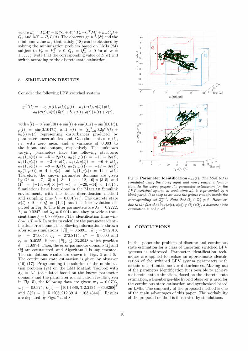
5 SIMULATION RESULTS

Consider the following LPV switched systems

y(3)(t) = −a0 (σ(t), ρ(t)) y(t)− a1 (σ(t), ρ(t)) y(t)

− a2 (σ(t), ρ(t)) y(t) + b0 (σ(t), ρ(t))u(t) + ε(t),

with u(t) = 3 (sin(10t) + sin(t) + sin(0.1t) + sin(0.01t)),

ρ(t) = sin(0.1047t), and ε(t) =∑2i=0 0.2y(i)(t) +

b0 (·) ν1(t) representing disturbances produced byparameter uncertainties and Gaussian noises ν1(t),ν2, with zero mean and a variance of 0.003 tothe input and output, respectively. The unknownvarying parameters have the following structure:a0 (1, ρ(t)) = −5 + 2ρ(t), a0 (2, ρ(t)) = −11 + 2ρ(t),a1 (1, ρ(t)) = −2 + ρ(t), a1 (2, ρ(t)) = −6 + ρ(t),a2 (1, ρ(t)) = −9 + 3ρ(t), a2 (2, ρ(t)) = −17 + 3ρ(t),b0 (1, ρ(t)) = 4 + ρ(t), and b0 (1, ρ(t)) = 14 + ρ(t).Therefore, the known parameter domains are givenby Ω1 = [−7,−3] × [−3,−1] × [−12,−6] × [3, 5], andΩ2 = [−13,−9] × [−7,−5] × [−20,−14] × [13, 15].Simulations have been done in the Matlab Simulinkenvironment, with the Euler discretization methodand sampling time h = 0.001[sec]. The discrete stateσ(t) : R → Q = 1, 2 has the time evolution de-picted in Fig. 6. The filter parameters are λ1 = 0.2222,λ2 = 0.0247 and λ3 = 0.0014 and they provide a tran-sient time ξ = 0.8889[sec]. The identification time win-dow is T = 5. In order to calculate the parameter identi-fication error bound, the following information is thrownafter some simulations, ‖f‖1 = 3.6391, ‖Ψ‖2 = 27.2013,

φ+ = 27.0659, η2 = 272.8114, ε+ = 9.6000 and

εθ = 0.4055. Hence, ‖θ‖2 ≤ 23.3948 which providesδ = 11.6974. Then, the error parameter domains Ω1

δ andΩ2δ are constructed, and Algorithm 1 is implemented.

The simulations results are shown in Figs. 5 and 6.The continuous state estimation is given by observer(16)-(17). Programming the solution of the minimiza-tion problem (24) on the LMI MatLab Toolbox withδA = 3.1 (calculated based on the known parameterdomains and the parameter identification results givenin Fig. 5), the following data are given: $1 = 0.0703,

$2 = 0.0374, L(1) = [161.1886, 312.2134,−86.8298]T

and L(2) = [115.1206, 212.3914,−103.4344]T

. Resultsare depicted by Figs. 7 and 8.

0100

200300

400

−20−15−10−505−14

−12

−10

−8

−6

−4

−2

0

2

4

6

Time [sec]a0 (σ(t), ρ(t))

a1(σ(t),ρ(t))

Ω1δ

Ω1

Ω2Ω2

δ

0100

200300

−30−25−20−15−10−505

−5

0

5

10

15

20

25

Time [sec]a2 (σ(t), ρ(t))

b0(σ(t),ρ(t))

Ω2δ

Ω2

Ω1

Ω1δ

Fig. 5. Parameter Identification θLS(t). The LSM (6) issimulated using the noisy input and noisy output informa-tion. In the above graphs the parameter estimation for theLPV switched system at each time kh is represented by ablack point. It is easy to see how the points remain inside the

corresponding set Ωσ(t)δ . Note that Ω1

δ ∩ Ω2δ 6= ∅. However,

due to the fact that θLS(σ(t), ρ(t)) 6∈ Ω1δ ∩Ω2

δ, a discrete stateestimation is achieved.

6 CONCLUSIONS

In this paper the problem of discrete and continuousstate estimation for a class of uncertain switched LPVsystems is addressed. Parameter identification tech-niques are applied to realize an approximate identifi-cation of the switched LPV system parameters withcertain uncertainties and/or disturbances. Making useof the parameter identification it is possible to achievea discrete state estimation. Based on the discrete stateestimation, a Luenberger-like hybrid observer is used forthe continuous state estimation and synthesized basedon LMIs. The simplicity of the proposed method is oneof the main advantages of this paper. The workabilityof the proposed method is illustrated by simulations.

10

0 20 40 60 80 100 120 140 160 180 200 220 240 260 280 3000

0.5

1

1.5

2

2.5

Time [sec]

σ(t)σ(t)

Fig. 6. Discrete State Estimation σ(kh). The discretestate estimation provided by Algorithm 1 is depicted in thetop graph. It is worth mentioning that it is only possi-ble to ensure the discrete state estimation after the timeT + ξ + ζ = 5.8899[sec] after each switching time.

0 20 40 60 80 100 120 140 160 180 200 220 240 260 280 300−40

−20

0

20

Time [sec]

0 20 40 60 80 100 120 140 160 180 200 220 240 260 280 300

−20

−10

0

10

0 20 40 60 80 100 120 140 160 180 200 220 240 260 280 300−10

0

10

20

x1x1

x2x2

x3x3

Fig. 7. Continuous State Estimation x(t).

0 20 40 60 80 100 120 140 160 180 200 220 240 260 280 300

0

5

10

15

20

25

30

35

40

Time [sec]

||e(t)||2

0 50 100 150 200 250 3000

1

2

3

4

Fig. 8. Continuous State Estimation Error Norm‖e(t)‖2.

Acknowledgements

The authors gratefully acknowledge the financial sup-port from CONACyT 151855, 209247, CONACyT209731 - CNRS 222629 Bilateral Cooperation ProjectMexico-France, and IPN-SIP 20130983. This work wasalso supported in part by the Government of RussianFederation (Grant 074-U01) and the Ministry of Ed-ucation and Science of Russian Federation (Project14.Z50.31.0031).

References

[1] F. J. Bejarano and L. Fridman. State exact reconstructionfor switched linear systems via a super-twisting algorithm.International Journal of Systems Science, 42(5):717–724,2011.

[2] V. I. Bogachev. Measure Theory I. Springer-Verlag, Berlin,Heidelberg, 2007.

[3] M. Fliess, C. Join, and W. Perruquetti. Real-time estimationof the switching signal for perturbed switched linear systems.In Proceedings of the 3rd IFAC Conference on Analysis andDesign of Hybrid Systems, pages 409–414, Zaragoza, Spain,2009.

[4] T. Floquet, D. Mincarelli, A. Pisano, and E. Usai. Continuousand discrete state estimation in linear switched systemsby sliding mode observers with residuals projection. InProceedings of the 4th IFAC Conference on Analysis andDesign of Hybrid Systems, pages 265–270, Eindhoven, TheNetherlands, 2012.

[5] R.W. Hamming. Digital Filters. Dover books on engineering.Dover Publications, Mineola, NY, 2007.

[6] M. Hanifzadegan and R. Nagamune. Smooth switching LPVcontroller design for lpv systems. Automatica, 50:1481–1488,2014.

[7] X. He, G.M. Dimirovski, and J. Zhao. Control of switchedLPV systems using common Lyapunov function method andan F-16 aircraft application. In 2010 IEEE InternationalConference on Systems Man and Cybernetics, pages 386–392,Istanbul, Turkey, 2010.

[8] R Isermann and M. Munchhof. Identification of DynamicSystems, An Introduction with Applications. Springer-Verlag,Berlin, 1st edition, 2011.

[9] H. Khalil. Nonlinear Systems. Prentice Hall, New Jersey,U.S.A., 2002.

[10] F. Lescher, J.-Y. Zhao, and P. Borne. Switching LPVcontrollers for a variable speed pitch regulated wind turbine.International Journal of Computers, Communications andControl, 1(4):73–84, 2006.

[11] D. Liberzon. Switching in Systems and Control. Systems andControl: Foundations and Applications. Birkhuser, Boston,MA, 2003.

[12] S. Lim and J.P. How. Modeling and H∞ control forswitched linear parameter-varying missile autopilot. IEEETransactions on Control Systems Technology, 11(6):830–838,Nov 2003.

[13] L. Liu, X. Wei, and Z. Liu. Switching LPV control for theair path system of diesel engines. In Chinese Control andDecision Conference, pages 4167–4172, Shangai, P.R. China,2008.

11

[14] L. Ljung. System Identification: Theory for the User. PrenticeHall Information and System Sciences Series, New Jersey,second edition, 1999.

[15] B. Lu and F. Wu. Switching LPV control designsusing multiple parameter-dependent Lyapunov functions.Automatica, 40:1973–1980, 2004.

[16] B. Lu, F. Wu, and S. W. Kim. Switching LPV control of anF-16 aircraft via controller state reset. IEEE Transactionson Control Systems Technology, 14(2):267–277, Mar 2006.

[17] J. Mohammadpour and C.W. Scherer. Control of LinearParameter Varying Systems with Applications. Springer, NewYork, 2012.

[18] A.M. Nagy, G. Mourot, B. Marx, J. Ragot, and G. Schutz.Systematic multi-modeling methodology applied to anactivated sludge reactor model. Industrial & EngineeringChemistry Research, 49(6):2790–2799, February 2010.

[19] N. Orani, A. Pisano, M. Franceschelli, A. Giua, and E. Usai.Robust reconstruction of the discrete state for a class ofnonlinear uncertain switched systems. Nonlinear Analysis:Hybrid Systems, 5(2):220–232, 2011.

[20] B. Ramaswami and K. Ramar. Transformation oftime-variable systems to canonical (phase-variable) form.IEEE Transactions on Automatic Control, 13(6):746–747,December 1968.

[21] H. Rıos, D. Efimov, J. Davila, T. Raıssi, L. Fridman, andA. Zolghadri. Non-minimum phase switched systems: Hosm-based fault detection and fault identification via volterraintegral equation. International Journal of Adaptive Controland Signal Processing, 2013. DOI: 10.1002/acs.2448.

[22] H. Rıos, D. Mincarelli, D. Efimov, W. Perruquetti, andJ. Davila. Discrete state estimation for switched LPV systemsusing parameter identification. In 2014 American ControlConference, pages 3243–3248, Portland, OR, USA, 2014.

[23] W.J. Rugh and J.S. Shamma. Research on gain scheduling.Automatica, 36:1401–1425, 2000.

[24] C.W. Scherer. Mixed H2/H∞ control for time-varying andlinear parametrically-varying systems. International Journalof Robust and Nonlinear Control, 6(9-10):929–952, 1996.

[25] J.S. Shamma. Analysis and design of gain scheduledcontrol systems. Ph.D. Thesis, Department of MechanicalEngineering, MIT, 1988.

[26] L. Silverman. Transformation of time-variable systems tocanonical (phase-variable) form. IEEE Transactions onAutomatic Control, 11(2):300–303, April 1966.

[27] L. Vu and D. Liberzon. Invertibility of switched linearsystems. Automatica, 44:949–958, 2008.

[28] L. Zhang, N. Cui, M. Liu, and Y. Zhao. Asynchronousfiltering of discrete-time switched linear systems with averagedwell time. IEEE Transactions on Circuits and Systems I,58(5):1109–1118, 2011.

[29] L. Zhang and P. Shi. L2−L∞ model reduction for switchedLPV systems with average dwell time. IEEE Transactionson Automatic Control, 53(10):2443–2448, 2008.

[30] K. Zhou and J.C. Doyle. Essentials of robust control.Prentice-Hall, 1998.

12