Contingent Claims Valuation - et.perso.eisti.fret.perso.eisti.fr/pdfs/CCV-2015-02-09.pdf ·...

IntroductionMono-Period

Binomial Model IContinuous Time Markets

Contingent Claims Valuation

Erik Taflin, EISTI

January 2010 version2015-02-09

Erik Taflin, EISTI QFRM M1 Cont Cl Val and IFI ING2



Outlines I

IntroductionSome different types of derivativesMarket ModelsArbitrage PricingFrictionless and Ideal Market

Mono-Period MarketProbabilistic ModelArbitrage and Equivalent Martingale MeasurePricing of Derivative Products




Outlines IIBinomial Model I

DefinitionPortfoliosArbitrage and Equivalent Martingale Measure (e.m.m.)Price of derivative and completness

Continuous Time MarketsOriginal Black-Scholes Model and FormulaThe greeks




Some different types of derivativesMarket ModelsArbitrage PricingFrictionless and Ideal Market

1. Introduction

• Financial Asset: Firstly, a contract, which only generate flows ofmoney is a financial assets. Secondly, a contract, which onlygenerate flows of other financial assets is also a financial asset.• Financial Derivative: Financial asset, whose price only dependson the value of other more basic underlying variables, such asStock prices, Bond prices, Temperature, Snow depth, . . .• (Non-financial) Derivatives ∃ since thousands of years: ForwardContracts on raw products, s.a. wheat• Synonyms in this course: Financial Derivative, Derivative,Derivative Security, Contingent Claim, . . .• Fundamental Problem: Find a fair price of a Contingent Claim(evaluation). Black, Merton and Scholes (∼1973)





• Role of Derivatives:

- Hedge (cover) risks for some

- Portfolio management and speculation for others

- Arbitraging for a small number





1.1 Some different types of derivatives

Underlying Assets: Spot price of a stock, Future price of a stock,Exchange rate ($/e, . . . ), . . . . Underlying Assets also calledPrimary AssetsA) ForwardForward (contract): Contract that stipulates that its holder canand shall buy the underlying for a predetermined amount K (thedelivery price) at a given future time T (the time of maturity).The delivery price K is determined such that the value of thecontract is zero at the contract dateForward Price: Let t0 be the contract date. Then, by definition,the Forward Price of the underlying at t0 for delivery at T is K .





B) Options• European Call Option: Contract that stipulates that its holdercan buy the underlying for a predetermined amount K (the strike)at a given future time T (the time of maturity or exercise date).• American Call Option: As European except that all exercisesdates t ≤ T are allowed.• Put Options: Substitute sell in place of buy in def. of Call• Pay-Off at exercise time te and price of underlying Ste :

- Call: (Ste − K )+

- Put: (K − Ste )+

• Other Options: Asian, Barrier, Caps, Floors, Swaptions,Straddle, Bermudan, Russian, . . .





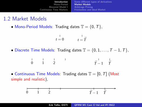
1.2 Market Models

• Mono-Period Models: Trading dates T = 0,T,| |

t = 0 t = T

• Discrete Time Models: Trading dates T = 0, 1, . . . ,T − 1,T,

| | | | | |

0 1 2 T −1 T

• Continuous Time Models: Trading dates T = [0,T ] (Mostsimple and realistic),

| | | | | |

0 1 2 T −1 T





1.3 Arbitrage Pricing

• An Arbitrage Portfolio in a financial market (with a risk-freeasset) is a self-financing portfolio θ, whose value Vt(θ) at datet ∈ T satisfies:

i) V0(θ) = 0

ii) VT (θ) ≥ 0

iii) P(VT (θ) > 0) > 0

• Arbitrage Free Market: @ an arbitrage portfolio; AOA• Arbitrage Pricing of Derivatives in a arbitrage free market ofunderlying assets: The price of a derivative is determined such thatthe extended market of underlying assets and the derivative isArbitrage Free





I Efficient Market Hypothesis:I asset prices reflect all information available in the marketI no one can earn excess returns with certainty.

I AOA:I is more general than Efficient Market Hypothesis, cf. certain

incomplete marketsI is a precise mathematical formulation of the fact that:

no one can earn excess returns with certainty.





1.4 Frictionless and Ideal Market

We make several simplifying hypotheses concerning the financialmarket (frictionless market):

I The number of financial assets is constant in time

I Asset prices take real values. No dividends are payed

I One can sell and buy any real number multiple of an asset

I Buy and sell prices are equal (i.e. no transaction costs)

I Lend and borrow interest rates are equal

I The price of an asset is independent of the amount one buyand sell (Price-taker market)

I All information is public

A more realistic market can be obtained by modifying the IdealMarket, with transaction costs and other frictions




Probabilistic ModelArbitrage and Equivalent Martingale MeasurePricing of Derivative Products

2. Mono-Period Market2.1 Probabilistic Model

• Trading dates: T = 0,T• Probability space: (Ω,P,F), Ω set of elementary events, P apriori probability, F σ-algebra of possible events• Usually, but not always: Ω = ω1, . . . , ωK, where K is thenumber of elementary events, pi = P(ωi ) > 0, F = subsets of Ω• N general Assets with prices S1, . . . ,SN (Quoted Spot Prices)and possibly one more asset, a risk-free Asset with deterministicprice S0.• Spot prices at t = 0 : S0 = (S1

0 , . . . ,SN0 ) ∈ RN if N assets;

S0 = (S00 , S

10 , . . . ,S

N0 ) ∈ RN+1 and S0

0 > 0, if N + 1 assets. Bydefault S0

0 = 1, if not specified differently.





• Spot prices at T : ST = (S1T , . . . ,S

NT ) is a random vector in RN

if N assets; ST = (S0T , S

1T , . . . ,S

NT ) is a random vector in RN+1 if

1 + N assets, S01 > 0,

• Interest Rate r , when S0 ∃: S0T = (1 + r)S0

0 , so 1 + r > 0• Portfolio: θi is the number of units of the i-th asset held in theportfolio θ. θ = (θ1, . . . , θN) ∈ RN if N assets.θ = (θ0, . . . , θN) ∈ R1+N if 1 + N assets• Value V(θ) of a prtf θ:

- at t = 0 : V0(θ) =∑

i θiS i

0 = θ · S0 ∈ R- at t = T : VT (θ) =

∑i θ

iS iT = θ · ST is random variable in R

• Gains from date 0 to date T on the investment V0(θ) in the prtfθ: G(θ) = VT (θ)− V0(θ) = θ · (ST − S0) is random variable in R• Return on the investment in the prtf θ: R(θ) = VT (θ)/V0(θ) ifV0(θ) 6= 0





• Discounted prices, gains and return, when risk-free asset withprice S0 ∃: S i

t = S it/S0

t , Vt(θ) = θ · S0t , G(θ) = VT (θ)− V0(θ),

R = VT (θ)/V0(θ)• Representation when Ω is a finite set:

V0(θ)

(VT (θ))(ωK)

(VT (θ))(ω1)

(VT (θ))(ω2)

...





• Matrix notation for calculations when Ω is a finite set:

- Let S and R be, when risk-free asset with price S0 ∃ theK × (1 + N) matrix and when risk-free asset with price S0 @the K × N matrix, with elements Sij = S j

T (ωi ) and

Rij = Sij/S j0 respectively. S is the price matrix and R the

matrix of returns.

- Given a prtf θ, with V0(θ)) 6= 0. Let Θ and ϑ be, whenrisk-free asset with price S0 ∃ the (1 + N)× 1 matrix andwhen risk-free asset with price S0 @ the N × 1 matrix, withelements Θi = θi and ϑi = θiS i

0/V0(θ)) respectively. Θ is theportfolio matrix and ϑ the portfolio fractions matrix.

- Let V be the K × 1 matrix with elements Vi = (VT (θ))(ωi ).

- Then V = SΘ and (R(θ))(ωi ) = (Rϑ)i for 1 ≤ i ≤ K .





2.2 Arbitrage and Equivalent Martingale Measure• An Arbitrage Portfolio (or an Arbitrage Opportunity) is aportfolio θ such that one of the following two statements A and Bis true:

A: The following three statements are true

i) V0(θ) = 0ii) VT (θ) ≥ 0iii) P(VT (θ) > 0) > 0

B: The following two statements are true

i) V0(θ) < 0ii) VT (θ) ≥ 0

• Caution: In this course the above definition is specific formono-period case• An Arbitrage Free Market is a market where @ an ArbitragePortfolio; (Also: Arbitraged Market, AOA)





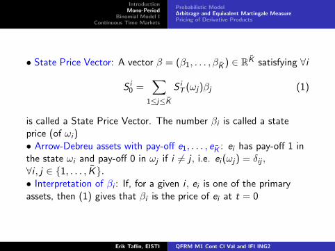
• State Price Vector: A vector β = (β1, . . . , βK ) ∈ RK satisfying ∀i

S i0 =

∑

1≤j≤KS iT (ωj)βj (1)

is called a State Price Vector. The number βi is called a stateprice (of ωi )• Arrow-Debreu assets with pay-off e1, . . . , eK : ei has pay-off 1 inthe state ωi and pay-off 0 in ωj if i 6= j , i.e. ei (ωj) = δij ,∀i , j ∈ 1, . . . , K.• Interpretation of βi : If, for a given i , ei is one of the primaryassets, then (1) gives that βi is the price of ei at t = 0





• Price Π0(X ) at date t = 0 of a general pay-off X at date T .Intuitively, since βi not always tradable: An asset with pay-offX (ωi )ei at date T has price X (ωi )βi at t = 0, so a price candidateis (justification in §3)

Π0(X ) =∑

1≤i≤KX (ωi )βi (2)

Caution: β not unique in general ⇒ Π0(X ) not unique in general

Theorem 2.1 (v1 of First Fundamental Th of Finance)

@ an arbitrage portfolio if and only if ∃ β such that βi > 0, ∀1 ≤ i ≤ K . Proof:





• Equivalent martingale Measure (E.M.M.) and Interest Rate:

- Suppose that ∃ state price vector β, with βi > 0 ∀i . Define rby

1/(1 + r) =∑

1≤i≤Kβi (3)

- r is the interest rate defined by a risk-free asset. In fact, Eq.(2) ⇒

Π0(1 + r) =∑

1≤i≤K(1 + r)βi = 1 (4)

- Define qi = (1 + r)βi and the measure Q by Q(ωi) = qi .Then qi > 0 and

∑1≤i≤K qi = 1, so Q is a probability

measure and P ∼ Q.





- Expected value w.r.t. Q is: EQ [X ] =∑

1≤i≤K X (ωi )qi . Eq.(2) ⇒

Π0(X ) = EQ

[X

1 + r

](5)

- Ingredients : Arbitrage Price, Q ∼ P and Pay-Off discountedto t = 0





• Interpretation of Q, when risk-free asset with price S0 ∃:

- S , the discounted prices are defined by: S it = S i

t/S0t for t ∈ T.

So S00 = S0

T = 1

- Eq. (5) gives

S i0 = EQ

[S iT

], 0 ≤ i ≤ N (6)

- Eq. (6) ⇒ S is a martingale under Q

• Definition of e.m.m. (in market with or without S0):

Definition 2.2An Equivalent Martingale Measure (e.m.m.) Q is a probabilitymeasure on (Ω,F) equivalent to P, such that for some r > −1and ∀i

S i0 = EQ

[S iT

1 + r

]. (7)





i) In general there is not a unique e.m.m., i.e. equation (7) for Qand r has not always a unique solution.ii) If Q and r is a solution of (7), then βi = qi/(1 + r), withqi = Q(ωi), defines a state price vector β satisfying (3).• First Fundamental Theorem of Finance: Theorem 2.1 gives

Theorem 2.3 (v2 of First Fundamental Th of Finance)

∃ an Equivalent Martingale Measure if and only if the market isarbitrage free





Corollary 2.4

In an arbitrage free market, we have for all interest rates r ande.m.m. Q solution of (7) and all portfolios θ that

V0(θ) = EQ

[VT (θ)

1 + r

]. (8)

• Vt(θ) portfolio price discounted to date 0 if S0 ∃: LetVt(θ) = Vt(θ)/S0

t . Corollary 2.4 ⇒

V0(θ) = EQ

[VT (θ)

]. (9)





2.3 Pricing of Derivative Products

We here introduce arbitrage pricing methods clarifying the validityand meaning of pricing formulas (2) and (5).• Derivative Product: A derivative is defined by its pay-off X atdate T , where X is any F-measurable r.v. (Only mono-periodcase)• Hedging Portfolio: A derivative X is hedgeable (or attainable) ifthere ∃ a prtf. θ s.t.

VT (θ) = X . (10)

Such θ is called a Hedging portfolio of X .• M: In the sequel M denotes the spot market defined by S andthe set of possible portfolios.





Example 2.5

We consider the mono-period market with interest rate r = 10%and two stocks S1 et S2 :

- Price at t = 0 : S10 = S2

0 = 100

- Price at t = T :

S1T (ω1) = 88, S1

T (ω2) = 110, S1T (ω3) = 132, (11)

S2T (ω1) = 132, S2

T (ω2) = 88, S2T (ω3) = 110. (12)

Find a hedging portfolio of a Put on S1 with strike 105.





Solution:The pay-off is X = (105− S1

T )+, so X (ω1) = 17, X (ω2) = 0 andX (ω3) = 0. The hedging portfolio θ shall satisfy VT (θ) = X .In matrix notation

X = SΘ, (13)

where

X =

1700

and S =

1110 88 1321110 110 881110 132 110

. (14)





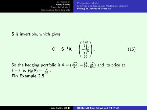
S is invertible, which gives

Θ = S−1X =

17033−17

661766

. (15)

So the hedging portfolio is θ = ( 17033 ,−17

66 ,1766 ) and its price at

t = 0 is V0(θ) = 17033 .

Fin Example 2.5.





• The value of Hedging Portfolios at t = 0 of X is unique:Suppose that the market M is Arbitrage Free. Let X be ahedgeable derivative and let θ and η be hedging portfolios of X .Then V0(θ) = V0(η). Let Q and r satisfy Eq. (7). Then

V0(θ) = EQ

[X

1 + r

]. (16)

Proof: Follows from (8) of Corollary 2.4.• M′: Let X be a derivative and x ∈ R. In next theorem M′denotes the market with prices S0 and x at t = 0 and prices ST

and X at t = T .





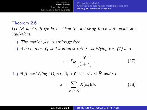
Theorem 2.6Let M be Arbitrage Free. Then the following three statements areequivalent:

i) The market M′ is arbitrage free

ii) ∃ an e.m.m. Q and a interest rate r , satisfying Eq. (7) and

x = EQ

[X

1 + r

]. (17)

iii) ∃ β, satisfying (1), s.t. βi > 0, ∀ 1 ≤ i ≤ K and s.t.

x =∑

1≤i≤KX (ωi )βi . (18)





Corollary 2.7

Let M be Arbitrage Free. If X is hedgeable, then the price x forwhich statement ii) of Theorem 2.6 holds true is unique.

• Thus, for a hedgeable derivative X , Theorem 2.6 and Corollary2.7 justify to call this unique price x , The Arbitrage Price of X . Itis denoted Π0(X ) and

Π0(X ) = EQ

[X

1 + r

], (19)

for any e.m.m. Q and a interest rate r , satisfying Eq. (7).





Example 2.8

We consider the mono-period market with interest rate r = 5%,two stocks S1 and S2 and three states ω1, ω2 and ω3 :

S1T

S10

(ω1) =42

31,

S1T

S10

(ω2) =21

31,

S1T

S10

(ω3) =21

62

andS2T

S20

(ω1) =21

124,

S2T

S20

(ω2) =42

31,

S2T

S20

(ω3) =168

31.

The a priori probability of ω1, ω2 and ω3 are 1/8, 3/8 and 4/8respectively.What is the price (at t = 0) of a Call on S2 with strike(150/31)S2

0 , obtained by using an e.m.m. Q? Also, find a hedgingportfolio of the Call. What is the price of the hedging portfolio?





Solution:Let qk = Q(ωk). The eq. EQ

[ST

]= S0 gives

EQ [ST ] = (1 + r)S0, which then gives

q1S iT (ω1) + q2S i

T (ω2) + q3S iT (ω3) = (1 + r)S i

0 i = 0, 1, 2.

With matrix notation we obtain

(R)t

q1

q2

q3

= (1 + r)

111

. (20)

Here

R =

2120

4231

21124

2120

2131

4231

2120

2162

16831

. (21)





The unique solution of (20) is

q1 =3

5, q2 =

3

10, q3 =

1

10. (22)

The pay-off of the Call is X = (S2T − 150

31 S20 )+, so X (ω1) = 0,

X (ω2) = 0 and X (ω3) = 1831 S2

0 . Its price at t = 0 is

EQ

[X

1 + r

]= q3

X (ω3)

1 + r=

12

217S2

0 . (23)





A hedging portfolio θ of the Call shall satisfy VT (θ) = X . In matrixnotation

X = SΘ = R

θ0S0

0

θ1S10

θ2S20

, where X =

00

1831 S2

0

. (24)

This gives θ0S0

0

θ1S10

θ2S20

= S2

0

−3600

8897124148

287

. (25)

We have V0(θ) = 12217 S2

0 , which, as it should be, is the same as thethe price given in (23). Fin Example 2.8.





• Complete Market: The market M is said to be Complete, when“all” derivatives are hedgeable.• Second Fundamental Theorem:

Theorem 2.9 (Second Fundamental Th of Finance)

The following three statements are equivalent:

i) The market M is arbitrage free and complete

ii) ∃ a unique e.m.m. Q

iii) ∃ a unique state price vector β s.t. ∀k βk > 0

Corollary 2.10

In an arbitrage free and complete market, every derivative X has aunique arbitrage price Π0(X ) at t = 0, given by (19).





• Pricing of a derivative X in an Incomplete Market: If X ishedgeable, then a unique arbitrage price Π0(X ) is given by (19)according to Corollary 2.7. As we shall see, there is no uniquearbitrage price, when X is not hedgeable.• Me : Let Me be the set of e.m.m. for the market M, which issupposed arbitrage free. So Me 6= ∅.• Possible arbitrage prices of X : Theorem 2.6 and formula (17)gives that for every Q ∈Me and corresponding interest rate r , apossible arbitrage price is given by

EQ

[X

1 + r

].

This leads to an interval of possible arbitrage prices.





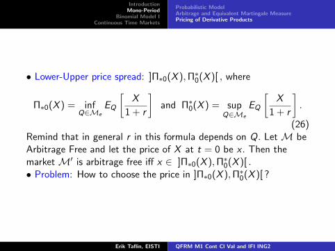
• Lower-Upper price spread: ]Π∗0(X ),Π∗0(X )[ , where

Π∗0(X ) = infQ∈Me

EQ

[X

1 + r

]and Π∗0(X ) = sup

Q∈Me

EQ

[X

1 + r

].

(26)Remind that in general r in this formula depends on Q. Let M beArbitrage Free and let the price of X at t = 0 be x . Then themarket M′ is arbitrage free iff x ∈ ]Π∗0(X ),Π∗0(X )[ .• Problem: How to choose the price in ]Π∗0(X ),Π∗0(X )[ ?





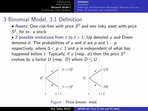
3 Binomial Model, 3.1 Definition• Assets: One risk-free with price S0 and one risky asset with priceS1, for ex. a stock• 2 possible evolutions from t to t + 1: Up denoted u and Downdenoted d . The probabilities of u and d are p and 1− prespectively, where 0 < p < 1 and p is independent of what hashappened before t. Typically, if u (resp. d) then the price S1

evolves by a factor U (resp. D) where D ≤ U :

u

d

S0t

(1+ r)S0t

(1+ r)S0t

t t +1

u

d

S1t

US1t

DS1t

t t +1

Figure : Price binom. mod.





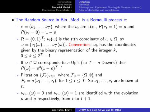
• The Random Source in Bin. Mod. is a Bernoulli process ν:

- ν = (ν1, . . . , νT ), where the νt are i.i.d., P(νt = 1) = p andP(νt = 0) = 1− p

- Ω = 0, 1T ; νt(ω) is the t:th coordinate of ω ∈ Ω, soω = (ν1(ω), . . . , νT (ω)). Convention: ωk has the coordinatesgiven by the binary representation of the integer k,0 ≤ k ≤ 2T − 1

- If ω ∈ Ω corresponds to n Up’s (so T − n Down’s) thenP(ω) = pn(1− p)T−n

- Filtration Ftt∈T, where F0 = Ω, ∅ andFt = σ(ν1, . . . , νt), for 1 ≤ t ≤ T . So ν1, . . . , νt are known att.

- νt+1(ω) = 0 and νt+1(ω) = 1 are identified with the evolutiond and u respectively, from t to t + 1.





• Information tree: one-to-one correspondence between states andfinal leaves

t = 0 t = 1 t = 2 t = 3 t = T − 1 t = Tω0

ω1

ωn

ωn+1

ωK−2

ωK−1

Figure : Information tree; Number of states K = 2T





• Path lattice: one-to-one correspondence between states ω andpaths

t = 0 t = 1 t = 2 t = 3 t = T − 1 t = T

Figure : Path lattice; Number of paths K = 2T





Example 3.1

t = 0 t = 1 t = 2 t = T

ω0 = (0,0,0)

ω1 = (0,0,1)ω2 = (0,1,0)

ω3 = (0,1,1)ω4 = (1,0,0)

ω5 = (1,0,1)ω6 = (1,1,0)

ω7 = (1,1,1)

Figure : Information tree, with T = 3, K = 8





2) Filtration:

- F0 = Ω, ∅.- F1 = σ(ν1). To find it, let A1(0) = ν−1

1 (0) andA1(1) = ν−1

1 (1), where ν−11 (B) is the inverse image of the

set B.

Then A1(0) = ω0, ω1, ω2, ω3,A1(1) = ω4, ω5, ω6, ω7

so F1 = σ(A1(0),A1(1)).

Since A1(0),A1(1) is a partition of Ω it follows that, attime t = 1 we can distinguish between events in A1(0) andevents in A1(1), but we can not distinguish between eventswithin A1(0) or events within A1(1).





- F2 = σ(ν1, ν2). Let A2(i , j) = ν−11 (i) ∩ ν−1

2 (j). Then

A2(0, 0) = ω0, ω1,A2(0, 1) = ω2, ω3,A2(1, 0) = ω4, ω5,A2(1, 1) = ω6, ω7,

(27)

so F2 = σ(A2(0, 0),A2(0, 1),A2(1, 0),A2(1, 1). Since theA2(i , j) defines a partition of Ω, at t = 2 one can distinguishbetween events which are in two different such sets, but notwithin the same set.

- F3 = σ(ν1, ν2, ν3). LetA3(i , j , k) = ν−1

1 (i) ∩ ν−12 (i) ∩ ν−1

3 (k). ThenA3(i , j , k) = (i , j , k). Explicitly,

A3(0, 0, 0) = ω0, . . . ,A3(1, 1, 1) = ω7.

So F3 is the set of all subsets of Ω.





3) Let X be a r.v. (later on it will be a derivative product)

- X is F0-measurable, i.e known at t = 0, means exactly that Xis constant on Ω, i.e. X (ω) = X (ω′) ∀ω, ω′ ∈ Ω

- X is F1-m. ⇔ X is constant on A1(0) and constant on A1(1).

- X is F2-m. ⇔ X is constant on each one of the setsA2(0, 0),A2(0, 1),A2(1, 0),A2(1, 1)

- X is F3-m. ⇔ X is arbitrary





• Number of Up’s: Let Nt be the number of Up’s up to date tincluded:

N0 = 0, Nt = ν1 + . . .+ νt , if t > 0. (28)

• Binomial Distribution: If 0 ≤ n ≤ t, then

P(Nt = n) =

(t

n

)pn(1− p)t−n.

• Price Distribution:

S1t = S1

0 UNt Dt−Nt

gives (for D 6= U), P(S1t = S1

0 UnDt−n) =

(t

n

)pn(1− p)t−n.

• Recall that:

E [Nt ] = tp and var [Nt ] = tp(1− p).





• Markov Process:S1t+1

S1t

are independent of S10 , ..,S

1t

• To sum up, the binomial price model is given by the filteredprobability space (Ω,P,F ,A), the two dimensional price process Sand the possible trading times t ∈ T = 0, . . . ,T, where

I Ω is the set of elementary events

I P is the a priori probability measure

I F = FT is the σ-algebra of all events

I A = (Ft)t∈T is the filtration





Example 3.2

U = 2 , D = 12 , p = 3

4 , S10 = 1 , T = 3 Reduced tree S1 :

1

2

12

4

1

14

8

2

12

18

Figure : Price path lattice, ω1 = (0, 0, 1), ω2 = (0, 1, 0) andω4 = (1, 0, 0).





P (ω4) = p(1− p)2 = 34

(14

)2= 3

64

P (ω2) = p(1− p)2 = 364

P (ω1) = p(1− p)2 = 34

(14

)2= 3

64

P (ω0) = (1− p)3 =(14

)3

ω7

ω6

ω5

ω4

ω3

ω2

ω1

ω0

P (S13 = 1

2) = P (ω1 , ω2 , ω4)

= 3 · 364

= 964

Figure : Information tree





3.2 Portfolios• A portfolio θ is given by:

I θit is the number of units held at time t of asset nr. i

I θt = (θ0t , θ

1t ) is the portfolio held at time t. θt is known at t,

i.e. is Ft-measurable

I θ = (θ0, θ1, ..., θT ) is the portfolio process. It is adapted tothe filtration (Ft)t∈T.

• Value (price) Vt(θ) of θ at t

Vt(θ) = θ0t S0

t + θ1t S1

t = θt · St

• Gains process G (θ); Gains Gt(θ) from 0 to t

Gt(θ) =∑

0≤s<t

θs · (Ss+1 − Ss)





• Discounted prices S = SS0 , i.e. S0

t = S0t

S0t

= 1 and S1t = S1

t

S0t

• Discounted value of θ at t : VT (θ) = Vt(θS0t

= θt · St .

• Discounted gains

Gt(θ) =∑

0≤s<t

θs · (Ss+1 − Ss)

• Self-financed portfolio

Definition 3.3A portfolio θ is self-financed iff

∀ t ∈ T, Vt(θ) = V0(θ) + Gt(θ) (29)





Theorem 3.4θ is self-financed iff

∀ t ∈ 0, . . . ,T − 1, θt · St+1 = θt+1 · St+1 (30)

Proof: By definition Vt+1(θ) = θt+1 · St+1. Suppose (30) true.Repeated use of the following equality then shows that θ isself-financed:

Vt+1(θ) = θt · St+1 = θt · St + θt · (St+1 − St) = Vt(θ) + θt · (St+1 − St)

If θ is self-financed then repeated use of this equality, with the lastmember = θt+1 · St+1, in the opposite direction proves that (30) istrue.

Theorem 3.5θ is self-financed iff ∀ t ∈ T, Vt(θ) = V0(θ) + Gt(θ).





3.3 Arbitrage and Equivalent Martingale Measure (e.m.m.)

Question for motivation of the introduction of e.m.m

• Binomial model T = 3, U = 2, D = 12 , r = 0, p = 3

4 , S10 = 1

• European Call: Strike K = 1 (at the money), Maturity T

1

2

12

4

1

14

8

2

12

18

Pay Off = X = (S1T −K)+ = (S1

T − 1)+

7 = X(ω7)

1 = X(ω3) = X(ω5) = X(ω6)

0 = X(ω1) = X(ω2) = X(ω4)

0 = X(ω0)

• What is the price of the Call at t = 0?Erik Taflin, EISTI QFRM M1 Cont Cl Val and IFI ING2




Answer:

• The price is 1327 . In fact

13

27= Q(S1

3 = 2) · 1 + Q(S13 = 8) · 7 = 3q2(1− q) + 7q3. (31)

Q is here an Equivalent Martingale Measure (e.m.m) given by

Q(S1t+1 = US1

t+1) ≡ q =1 + r − D

U − D=

1− 1/2

2− 1/2=

1

3. (32)





• Arbitrage Opportunity (OA) and Arbitrage Portfolio in theBinomial financial market

Definition 3.6An Arbitrage Portfolio is a self-financing portfolio θ, whose valueVt(θ) at date t ∈ T satisfies:

i) V0(θ) = 0

ii) VT (θ) ≥ 0

iii) P(VT (θ) > 0) > 0

• AOA ⇔ @ OA ⇔ Arbitrage free market

Theorem 3.7The Binomial financial market is arbitrage free iff

D < 1 + r < U or D = 1 + r = U.





Lemma 3.8The following two statements are equivalent:

1. The Binomial market is arbitrage free

2. Every mono-period sub-market of the Binomial market isarbitrage free





Proof:• Suppose first that there exists a mono-period sub-market with anOA

ω2T−1

ω1

ω0

etats ∈ Ω0Ft

t0 t0 + 1Sous-Modele de t0 a t0 + 1avec OA permet la constructiond’un portefeuille d’arbitrage de t0 a t = T





θ0 = · · · = θt0−1 = 0

θt0 · St0= 0

θt0 · St0+1 ≥ 0

E[θt0 · St0+1

]> 0

(33)

θt0+1 = (θ0t+1, 0) = · · · = θT = (θ0

T , 0) all invested in the bankaccount.⇒ θ is an arbitrage portfolio.





• Suppose then that there does not exist a mono-periodsub-market with an OA. Let θ be a self-financed portfolio suchthat VT (θ) ≥ 0.

VT (θ) ≥ 0

t = t0 t = T





• Then VT−1(θ) ≥ 0, (or otherwise there exists an arbitrageportfolio from T − 1 to T )• So, by iteration VT (θ) ≥ 0, VT−1(θ) ≥ 0, . . . , V0(θ) ≥ 0.• Let θ be such that V0(θ) = 0. Since V1(θ) ≥ 0, we must haveV1(θ) = 0 (if not ∃ OA). Similarly

V1(θ) = 0 ⇒ V2(θ) = 0 ⇒ · · ·VT (θ) = 0

⇒ @ arbitrage portfolio θ.





• e.m.m.; Equivalent Martingale Measure in the Binomial financialmarket

Definition 3.9An e.m.m. is a probability measure Q s.t.Q ∼ P and S = S

S0 , is a Q martingale, i.e.

St = EQ

[St+1|Ft

], for all t = 0, 1, ...,T . (34)





• Find an e.m.m; Q ∼ P and (34) ⇔

S1t (ω)

(1 + r)t= EQ

[St+1

(1 + r)t+1|Ft

](ω)

⇔ S1t (ω) = qt(ω)

S1t (ω)U

(1 + r)+ (1− qt(ω))

S1t (ω)D

(1 + r)

⇔ qt(ω) = q ≡ 1 + r − D

U − D, if U > D and 0 < qt(ω) < 1 if U = D.

Here q is the probability under the mono-periode e.m.m.

Theorem 3.10For the Binomial financial market there exists an e.m.m. iff

D < 1 + r < U or D = 1 + r = U.





Corollary 3.11

For the Binomial financial market there exists an e.m.m. iff there isAOA

• Price of a self-financed portfolio θ:V (θ) is a Q-martingale, i.e.

Vt(θ) = EQ

[Vt+1(θ)|Ft

].

In fact, since θ is self-financed θt+1 · St+1 = θt · St+1 and since θtis Ft-measurable:

EQ

[Vt+1(θ)|Ft

]= EQ

[θt+1 · St+1|Ft

]= EQ

[θt · St+1|Ft

]

=∑

i

θitE[S it+1|Ft

]=∑

i

θit Sit = Vt(θ). (35)





3.4 Price of a derivative and completness

• A European Derivative is a contract, which determines thepay-off X (ω) for all ω ∈ Ω at the exercise date T . T coincide withthe maturity date.⇒ Bijective relation between real r.v. X on Ω and EU derivatives.• Hedging portfolio θ of an EU derivative X is a self-financedportfolio θ s.t. VT (θ) = X . X is said to be hedgeable.• Consider the cases for which there is AOA

1. D = 1 + r = U

2. D < 1 + r < U

What are the hedgeable EU derivatives X ?





1) D = 1 + r = U ⇒ S1t = S1

0 S0t

⇒ Vt(θ) = S0t (θ0

t + θ1t S1

0 )θ self-financed ⇔ ∀ 0 ≤ t ≤ T − 1, θtSt+1 = θt+1St+1

⇔ θ0t S0

t+1 + θ1t S1

0 S0t+1 = θ0

t+1S0t+1 + θ1

t+1S10 S0

t+1

⇔ θ0t + θ1

t S10 = θ0

t+1 + θ1t+1S1

0

⇒ by recursion in t that θ0t + θ1

t S10 = V0(θ)

⇒ Vt(θ) = V0(θ)S0t

⇒ Only deterministic X are hedgeable !!





2) D < 1 + r < U. Let X be an arbitrary r.v. on Ω. Try to find θself-financed and with VT (θ) = X .

X(ω2T−1)

X(ω2T−2)

X(ω3)

X(ω2)X(ω1)

X(ω0)

V (θ)(ω2T−1)2T − 2

V (θ)(ω3)2

V (θ)(ω1)0

Figure : Replace 2T by 2T





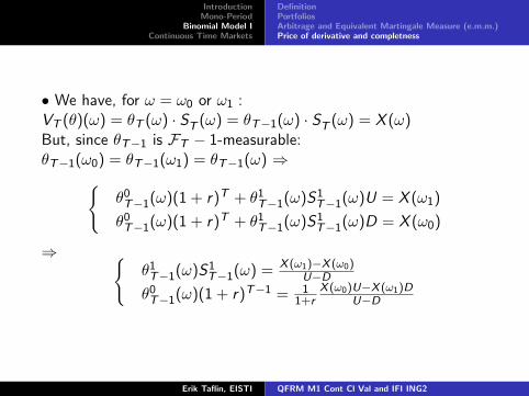
• We have, for ω = ω0 or ω1 :VT (θ)(ω) = θT (ω) · ST (ω) = θT−1(ω) · ST (ω) = X (ω)But, since θT−1 is FT − 1-measurable:θT−1(ω0) = θT−1(ω1) = θT−1(ω) ⇒

θ0T−1(ω)(1 + r)T + θ1

T−1(ω)S1T−1(ω)U = X (ω1)

θ0T−1(ω)(1 + r)T + θ1

T−1(ω)S1T−1(ω)D = X (ω0)

⇒ θ1T−1(ω)S1

T−1(ω) = X (ω1)−X (ω0)U−D

θ0T−1(ω)(1 + r)T−1 = 1

1+rX (ω0)U−X (ω1)D

U−D





• Same method for ω = ω2 or ω3

• Same method for ω = ω4 or ω5

• etc. same method up to ω = ω2T−2 or ω2T−1

• Then by iteration from T − 1 to T − 2, . . . , from t = 1 to t = 0.• ⇒ All EU derivatives X are hedgeable.





• Complete Market: A financial market is said to be complete if allderivatives are hedgeable. We have proved

Theorem 3.12For the Binomial Market the following statements are equivalent

I The Market is arbitrage free and complete

I D < 1 + r < U

I ∃ a unique e.m.m. Q

• Π(X ), Arbitrage price of X : Let θ be a hedging portfolio of X .For such θ, V (θ) is independent of θ, so we define

∀ t ∈ T Πt(X ) = Vt(θ). (36)

In the sequel price = arbitrage price• Π(X ), Discounted price of X : Πt(X ) = Πt(X )/S0

t .





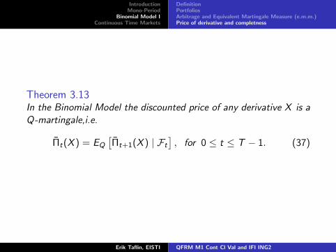
Theorem 3.13In the Binomial Model the discounted price of any derivative X is aQ-martingale,i.e.

Πt(X ) = EQ

[Πt+1(X ) | Ft

], for 0 ≤ t ≤ T − 1. (37)





Example 3.14

Prices for all ω and t in (31)

1

2

12

4

1

14

8

2

12

18

Price of X Pay Off = X = (S1T −K)+ = (S1

T − 1)+

7 = X(ω7)

1 = X(ω3) = X(ω5) = X(ω6)

0 = X(ω1) = X(ω2) = X(ω4)

0 = X(ω0)

1327

119

19

3

13

0





Example 3.15 (Barrier)

Let T = 3, r = 110 , U = 5

4 , D = 45 , S1

0 = 400, p = 34 . Find the

price at t = 0 of a Barrier Option of the type Down-And-Out Callwith

Barrier H = 350, Strike K = 450.

N.B : The Pay Off at T in the state ω is given by

X (ω) =

0 if min0≤t≤T S1

t (ω) < H

(S1T (ω)− K )+ if min0≤t≤T S1

t (ω) ≥ H(38)

We also have, denoting by 1A the caracteristic function of a set A :

X = (S1T − K )+ 1min0≤t≤T S1

t ≥H. (39)





Solution: q = 1+r−DU−D =

1110− 4

554− 4

5

. So q = 23

400

500

320

635

400

256

31354

= 781, 24

500

320

10245

= 204, 8

t = 0 t = 1 t = 2 t = 3 = T

S1t

350 = H





400

500

320

635

400

400

256

31254

= 781, 25

500

500

500

320

320

320

10245

= 204, 8

Information tree with S1

PAY-OFF in ω

(31254

− 450)+ = 13254

(ω7)

(500− 450)+ = 50 (ω6)

50 (ω5)

0 (ω4)

0 (ω3)

0 (ω2)

0 (ω1)

0 (ω0)





• Price at t = 0 :

Π0(X ) = EQ

[X

S0T

]=

1

(1 + r)TEQ [X ]

1

(1 + r)TEQ [X ] =

(10

11

)3(Q(ω5)50 + Q(ω6)50 + Q(ω7)

1325

4

)

=

(10

11

)3(2 · 50q2(1− q) +

1325

4q3

)

=

(10

11

)3(

100 ·(

2

3

)2

(1

3) +

1325

4·(

2

3

)3)

=

(10

33

)3

(400 + 2 · 1325) ≈ 84.87.





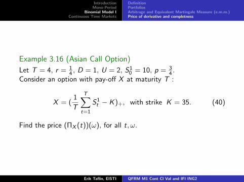
Example 3.16 (Asian Call Option)

Let T = 4, r = 14 , D = 1, U = 2, S1

0 = 10, p = 34 .

Consider an option with pay-off X at maturity T :

X = (1

T

T∑

t=1

S1t − K )+, with strike K = 35. (40)

Find the price (ΠX (t))(ω), for all t, ω.





Before studying the price of the option, we note that the pay-off Xis path dependant.

10

20

10

40

20

10

80

40

20

10

160

80

40

20

10

⇒ 1T

∑Tt=1 S

1t = 220

4

⇒ 1T

∑Tt=1 S

1t = 150

4





S10 = 10

20

10

40

20

20

10

80

40

40

20

10

20

20

40

160

8080

4080

4040

20

10

2020

4020

4040

80

ω ∈ Ω ; Ω = ω0, ω1, ..., ω15 K = 35

Arbre des prix S1t (ω)





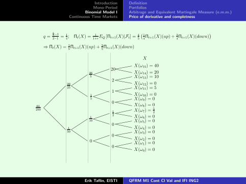
S14(ω)

14

∑4t=1 S

1t (ω) X = (1

4

∑4t=1 S

it −K)+

S14(ω15) = 160 300

4= 75 X(ω15) = 40

S14(ω14) = 80 220

4= 55 X(ω14) = 20

S14(ω13) = 80 180

4= 45 X(ω13) = 10

S14(ω12) = 40 140

4= 35 X(ω12) = 0

S14(ω11) = 80 160

4= 40 X(ω11) = 5

S14(ω10) = 40 120

4= 30 X(ω10) = 0

S14(ω9) = 40 100

4= 25 X(ω9) = 0

S14(ω8) = 20 80

4= 20 X(ω8) = 0

S14(ω7) = 80 150

4= 75

2X(ω7) =

52

S14(ω6) = 40 110

4= 55

2X(ω6) = 0

S14(ω5) = 40 90

4= 45

2X(ω5) = 0

S14(ω4) = 20 70

4= 35

2X(ω4) = 0

S14(ω3) = 40 80

4= 20 X(ω3) = 0

S14(ω2) = 20 60

4= 15 X(ω2) = 0

S14(ω1) = 20 50

4= 25

2X(ω1) = 0

S14(ω0) = 10 40

4= 10 X(ω0) = 0





61250

2925

150

265

15

0

110

20

2

1

0

0

0

0

12

q =54−1

2−1= 1

4; Πt(X) = 1

1+rEQ [Πt+1(X)|Ft] =

45

(14Πt+1(X)(up) + 3

4Πt+1(X)(down)

)

⇒ Πt(X) = 15Πt+1(X)(up) + 3

5Πt+1(X)(down)

X

X(ω15) = 40

X(ω14) = 20X(ω13) = 10

X(ω12) = 0X(ω11) = 5

X(ω10) = 0X(ω9) = 0

X(ω8) = 0

X(ω0) = 0

X(ω1) = 0X(ω2) = 0

X(ω3) = 0X(ω4) = 0

X(ω5) = 0X(ω6) = 0

X(ω7) =52




Original Black-Scholes Model and FormulaThe greeks

4 Continuous Time Markets

• Aim: Introduce the model of Black, Merton and Scholes and itsgeneralizations• Why Continuous time models?

- Assets are (in many cases) quoted at high frequency andwithout interruption; Ex: Foreign Exchange rates andStock-indices⇒ Almost continuously quoted

- A robust discrete time model must give predictions almostindependent of the time increment ∆, when ∆ is small:

| | | | | |

0 t t +Δ

⇒ Continuous limit ∃





- Quotes are not equidistant in reality:

| | | | | | | | | | || | | | | |

⇒ Quotes can be considered as a sample of a ContinuousTime Process

- Technical reasons:Discrete mathematics complicatedTheory of continuous time processes ∃ and computationaleasier (Stochastic integration, Ito’s calculus, Girsanov’stransformation, . . . )





4.1 Original Black-Scholes ModelStock price model• Trading dates: T = [0,T ]• Random source: A one dimensional Brownian motion W isdefined on a (complete) probability space (Ω,P,F), where P isthe a priori probability measure.• Filtration: Ftt∈T generated by W (and the null-sets); F = FT

• Two assets: A Risk-free bank account, with price process

S0t = S0

0 exp(rt) (41)

and a Risky stock with price process, which is an “exponentialBrownian”

S1t = S1

0 exp(σWt + (µ − 1

2σ2)t), (42)

where r , µ, σ ∈ R and σ 6= 0. S1t /S1

0 is log-normal; ln(S1t /S1

0 ) isN ((µ − 1

2σ2)t, σ2t)





• SDEs (Stochastic Differential Equation) by Ito’s lemma:

dS0t = rS0

t dt (43)

dS1t = S1

t µdt + S1t σdWt . (44)

Here r is the (continuous compounded) spot interest rate, µ thedrift and σ the volatility.• Discounted price S : S i = S i/S0

dS0t = 0 (45)

dS1t = S1

t (µ − r)dt + S1t σdWt . (46)

Exercise 4.1Let γ = µ−r

σ and ξt = exp(−γWt − 12γ

2t). Establish that ξS is a

P-martingale. (N.b. γ is called the market price of risk).





Portfolio• The portfolio θ = (θ0, θ1) :

- θ0t is the number of units of the risk-free asset held at time t

- θ1t is the number of units of the risky asset held at time t

- θ0t and θ1

t are known at time t, i.e. they are Ft-measurable.

- θt = (θ0t , θ

1t ) is the instantaneous portfolio at t.

• Price process V (θ) of a portfolio θ:

Vt(θ) = θt · St , t ∈ T. (47)

• Discounted Price process V(θ) of a portfolio θ: (Discounted todate 0)

Vt(θ) = Vt(θ)/S0t . (48)

Obviously Vt(θ) = θt · St .





• Gains process G(θ) of prtf. θ: Sum of the gains from date 0 upto date t

Gt(θ) =

∫ t

0θs · dSs , t ∈ T. (49)

Warning: To be rigorous, one should here introduce a set ofadmissible portfolios, such that the gains process is well-definedand such that the model is arbitrage free (excluding for exampledoubling strategies). This is outside the scope of this course andwe shall just suppose that the prtf. is sufficiently integrable oruniformly bounded from below, as to guarantee these properties.• Discounted Gains process G(θ) of prtf. θ:

Gt(θ) =

∫ t

0θs · dSs , t ∈ T. (50)

• Self-financing prtf. θ is a prtf. where the changes in its priceonly comes from variations in the asset prices, i.e.

Vt(θ) = V0(θ) + Gt(θ), ∀t ∈ T. (51)Erik Taflin, EISTI QFRM M1 Cont Cl Val and IFI ING2




Exercise 4.2Establish that the definition of a self-financing prtf. by formula(51) is equivalent to

Vt(θ) = V0(θ) + Gt(θ), ∀t ∈ T. (52)





Black-Scholes Equation• Simple EU derivative X , i.e.

X = f (S1T ), for some f

• Hedging prtf. θ of X :

VT (θ) = X , for some self-fin. prtf. θ

• To construct the hedging prtf. θ of X we try the ansatz: Thereis a function F ∈ C 1,2([0,T [ × ]0,∞[ ) s.t.

Vt(θ) = F (t,S1t ), ∀t ∈ T (53)

andF (T , x) = f (x), ∀x > 0. (54)

Introduce: F (t, x) = ∂F (t, x)/∂t, F ′(t, x) = ∂F (t, x)/∂x andF′′

(t, x) = ∂2F (t, x)/∂x2.Erik Taflin, EISTI QFRM M1 Cont Cl Val and IFI ING2




Differentiation of the l.h.s. of (53) gives, since θ is self-fin.:

dVt(θ) = θt · dSt = (rS0t θ

0t + µS1

t θ1t )dt + σS1

t θ1t dWt

= (rVt(θ) + (µ − r)S1t θ

1t )dt + σS1

t θ1t dWt

(55)

(53) and (55) give,

dVt(θ) = (rF (t,S1t ) + (µ − r)S1

t θ1t )dt + σS1

t θ1t dWt (56)

Differentiation of the r.h.s. of (53) gives, by Ito’s lemma,∀t ∈ [0,T [ :

dF (t, S1t ) = (F (t, S1

t ) + µS1t F ′(t,S1

t ) +1

2σ2(S1

t )2F′′

(t,S1t ))dt

+ σS1t F ′(t,S1

t )dWt .

(57)





Identification of (56) and (57) gives, first

θ1t = F ′(t,S1

t ), (58)

and then

rF (t,S1t )+(µ−r)S1

t θ1t = F (t,S1

t )+µS1t F ′(t, S1

t )+1

2σ2(S1

t )2F′′

(t,S1t ).

(59)• Eqs. (59) and (54) give the Black-Scholes Equation:∀ (t, x) ∈ T×]0,∞[,

∂∂t F (t, x) + rx ∂

∂x F (t, x) + 12σ

2x2 ∂2

∂x2 F (t, x) = rF (t, x),

F (T , x) = f (x), ∀x > 0.(60)

• The hedging prtf. θ is given by (58)

θ1t = F ′(t, S1

t )

θ0t = 1

S0t

(F (t,S1

t )− F ′(t, S1t )S1

t

).

(61)





A special case of the Feynman-Kac formula gives the solution ofthe B-S eq.:

Theorem 4.3(Under certain conditions on f ). If

F (t, x) = e−r(T−t)

∫ ∞

−∞f (xey )

1√2πσ2(T − t)

exp

(−(y − (T − t)(r − 1

2σ2))2

2σ2(T − t)

)dy ,

(62)

where (t, x) ∈ [0,T [ × ]0,∞[ , then F is the solution of the B-SEq. (60) and θ defined by (61) is a hedging prtf. of X = f (S1

T ).

Proof:





Black-Scholes Formula for a Call• Let f be the pay-off of a EU Call with strike K > 0 :

f (x) = (x − K )+, x > 0 (63)

and let C be the solution of the B-S eq. given by formula (62).Then

C(t, x) = e−r(T−t)∫ ∞−∞

(xey − K)+1√

2πσ2(T − t)exp

(−

(y − (T − t)(r − 12σ2))2

2σ2(T − t)

)dy

= e−r(T−t)∫ ∞

ln(K/x)(xey − K)

1√2πσ2(T − t)

exp

(−

(y − (T − t)(r − 12σ2))2

2σ2(T − t)

)dy.

(64)

We make the substitution

z = −y − (T − t)(r − σ2/2)

σ√

T − t, so y = −zσ

√T − t+(T−t)(r−σ2/2).





Let

z0 =ln(x/K ) + (T − t)(r − σ2/2)

σ√

T − t.

Formula (64) now gives

C (t, x) = e−r(T−t)

∫ z0

−∞

(x exp(−zσ

√T − t + (T − t)(r − σ2/2))− K

) e−z2

2√2π

dz .

(65)Let

I1(t, x) = e−r(T−t)

∫ z0

−∞x exp(−zσ

√T − t + (T − t)(r − σ2/2))

e−z2

2√2π

dz

and

I2(t, x) = −Ke−r(T−t)

∫ z0

−∞

e−z2

2√2π

dz .

ThenC (t, x) = I1(t, x) + I2(t, x).

Let N be the normal (0, 1) pdf (probability distribution function).





It follows that

I1(t, x) = x e−r(T−t)

∫ z0

−∞exp(−zσ

√T − t + (T − t)(r − σ2/2))

e−z2

2√2π

dz

= x

∫ z0

−∞exp

(− (z + σ

√T − t)2

2

)dz√2π

= x N(z0 + σ√

T − t ).

For I2 it follows that

I2(t, x) = −Ke−r(T−t)N(z0).

To sum up, introduce τ = T − t, d1(τ) = z0 + σ√τ and d2(τ) = z0, i.e.

d1(τ) =1

σ√τ

(lnx

K+ τ(r +

σ2

2)) (66)

d2(τ) =1

σ√τ

(lnx

K+ τ(r − σ2

2)), (67)

then (65) gives the Black-Scholes Formula for the price of a EU Call

C (t, x) = xN(d1(τ))− Ke−rτN(d2(τ)). (68)





0.25 0.5 0.75 1 1.25 1.5 1.75 2x

0.25

0.5

0.75

1

1.25

1.5

1.75

2C

Figure : Price C (0, x). Here T = 1, K = 1, r = 1/10 and σ = 4/10Erik Taflin, EISTI QFRM M1 Cont Cl Val and IFI ING2




1 2 3 4 5 6 7 8x

1

2

3

4

5

6

7

8C

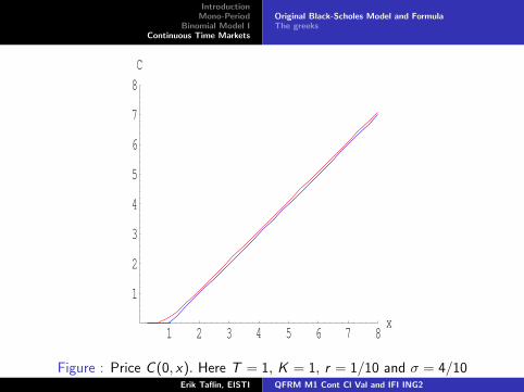
Figure : Price C (0, x). Here T = 1, K = 1, r = 1/10 and σ = 4/10Erik Taflin, EISTI QFRM M1 Cont Cl Val and IFI ING2




• Call-Put relation: Let P(T , x) = (K − x)+. Then

C (T ,S1T )− P(T , S1

T ) = S1T − K .

The arbitrage price at time t of each side then gives

C (t, S1t )− P(t,S1

t ) = S1t − Ke−r(T−t). (69)

Since this is true for all values of S1t , we obtain the Call-Put

relationC (t, x)− P(t, x) = x − Ke−r(T−t), (70)

for x > 0.• Price of a Put P(t, x) is obtained from formulas (68) and (70)and the relation 1− N(z) = N(−z)

P(t, x) = −xN(−d1(τ)) + Ke−rτN(−d2(τ)). (71)

for x > 0.Erik Taflin, EISTI QFRM M1 Cont Cl Val and IFI ING2




Example 4.4

Consider a standard B-S market, with annual interest rater = 3.5% and annual volatility σ = 30%. The stock price is 132etoday. What is the price today of a Call and a Put, with 9 monthsto maturity and strike 125?Let t be today. We have τ = 3/4Y and according to (66) and (67):d1(τ) = 1

3/10√

3/4(ln (132/125) + 3/4(35/1000 + (3/10)2/2)) ≈

0.440665 and d2(τ) =1

3/10√

3/4(ln (132/125) + 3/4(35/1000− (3/10)2/2)) ≈ 0.180858.

N(d1(τ)) ≈ 0.670272 and N(d2(τ)) ≈ 0.57176. Formula (68) givesC (t, 132) ≈ 18, 8576. The Call-Put parity relation (70) then givesP(t, 132) ≈ 8.61903.





4.2 The greeks• B-S model is complete, so by definition every derivative ishedgeable• However, in practice a hedge is in general only approximate forseveral reasons, as1) The portfolio can not be re-balanced continuously in time.2) The underlying price model, here the original B-S model, is onlyan approximation of the real price dynamics.3) The model parameters are only determined with a certainaccuracy.• Let F be the price function (here given by B-S eq. (60)) of asimple EU derivative X and let θ be an approximate hedging prtf.,s.t. its value at time t is a function of the stock price S1

t . Then theprice difference p at t of derivative and hedge is:

p(t, S1t ) = F (t,S1

t )− Vt(θ). (72)





• p is also a function of the model parameters r , µ and σ, if this isthe case for θ. Sensitivities of derivative price F (t, x), w.r.t.variations in t, x , r and σ needed;• “Greeks” for a Call F (t, x) = C (t, x) :

Delta ∆ =∂C (t, x)

∂x= N(d1) > 0, for x > 0. (73)

Gamma Γ =∂2C (t, x)

∂x2=

1

xσ√τ

N ′(d1) > 0, for x > 0. (74)

(So, the Call-price is strictly concave.)

Theta Θ =∂C

∂t= − xσ

2√τ

N ′(d1)−Ke−rτ r N(d2) < 0, for x > 0,

(75)where τ = T − t. (So C is increasing in τ .)





Vega V =∂C

∂σ= x√τ N ′(d1) > 0, for x > 0. (76)

Rho ρ =∂C

∂r= Kτe−rτ N(d2) > 0, for x > 0. (77)

• ∆, Γ and Θ satisfies, for a simple derivative with price F (seeB-S eq. (60)) :

Θ + rx∆ +1

2σ2x2Γ− rF = 0. (78)





Example 4.5

In the situation of Example 4.4, what are today the hedgingportfolios of the Call and the Put respectively?The hedging prtfs. are obtained from (61). Let x = 132. In thecase of the Call, eq. (73) gives

θ1t = N(d1) ≈ 0.670272 stocks

andθ0t S0

t = C (t, x)− N(d1)x ≈ −69.6184 e.


Contingent Claims Valuation - et.perso.eisti.fret.perso.eisti.fr/pdfs/CCV-2015-02-09.pdf ·...

Documents

Transcript of Contingent Claims Valuation - et.perso.eisti.fret.perso.eisti.fr/pdfs/CCV-2015-02-09.pdf ·...