CONTINENTAL SCALE VARIABILITY IN ECOSYSTEM · PDF fileCONTINENTAL SCALE VARIABILITY IN...

251

Ecological Monographs, 67(2), 1997, pp. 251–271q 1997 by the Ecological Society of America

CONTINENTAL SCALE VARIABILITY IN ECOSYSTEM PROCESSES:MODELS, DATA, AND THE ROLE OF DISTURBANCE

DAVID S. SCHIMEL,1 VEMAP PARTICIPANTS,2 AND B. H. BRASWELL3

1National Center for Atmospheric Research, P.O. Box 3000, Boulder, Colorado 80307-3000 USA and Natural ResourcesEcology Laboratory, Colorado State University, Fort Collins, Colorado 80523 USA

2Department of Environmental Sciences, University of Virginia, Charlottesville, Virginia 22903 USA: W. Emanuel, B.Rizzo, T. Smith; Department of Plant and Animal Sciences, University of Sheffield, P.O. Box 601, Sheffield S10 2UQ, UK:

F. I. Woodward; National Center for Atmospheric Research, P.O. Box 3000, Boulder, Colorado 80307-3000 USA: H.Fisher, T. G. F. Kittel, R. McKeown, T. Painter4, N. Rosenbloom; Natural Resources Ecology Laboratory, Colorado State

University, Fort Collins, Colorado 80523 USA: D. S. Ojima, W. J. Parton; The Ecosystems Center, Marine BiologicalLaboratory, Woods Hole, Massachusetts 02543 USA: D. W. Kicklighter, A. D. McGuire, J. M. Melillo, Y. Pan; Universityof Lund, ostra Vallsatian 14, 22361 Lund, Sweden: A. Haxeltine, C. Prentice, S. Sitch; University of Montana, Missoula,

Montana 59812 USA: K. Hibbard, R. Nemani, L. Pierce, S. Running; USDA Forest Service, Oregon State University, 3200SW Jefferson Way, Corvallis, Oregon 97333 USA: J. Borchers, J. Chaney, R. Neilson (institutions are listed alphabetically,

participants are alphabetized within group)3Institute for Earth Oceans and Space, The University of New Hampshire, Durham, New Hampshire 03824 USA and

National Center for Atmospheric Research, Boulder, Colorado 80307-3000 USA

Abstract. Management of ecosystems at large regional or continental scales and de-termination of the vulnerability of ecosystems to large-scale changes in climate or atmo-spheric chemistry require understanding how ecosystem processes are governed at largespatial scales. A collaborative project, the Vegetation and Ecosystem Modeling and AnalysisProject (VEMAP), addressed modeling of multiple resource limitation at the scale of theconterminous United States, and the responses of ecosystems to environmental change. Inthis paper, we evaluate the model-generated patterns of spatial variability within and be-tween ecosystems using Century, TEM, and Biome-BGC, and the relationships betweenmodeled water balance, nutrients, and carbon dynamics. We present evaluations of modelsagainst mapped and site-specific data. In this analysis, we compare model-generated patternsof variability in net primary productivity (NPP) and soil organic carbon (SOC) to, respec-tively, a satellite proxy and mapped SOC from the VEMAP soils database (derived fromUSDA-NRCS [Natural Resources Conservation Service] information) and also comparemodeled results to site-specific data from forests and grasslands. The VEMAP modelssimulated spatial variability in ecosystem processes in substantially different ways, reflect-ing the models’ differing implementations of multiple resource limitation of NPP. Themodels had substantially higher correlations across vegetation types compared to withinvegetation types. All three models showed correlation among water use, nitrogen avail-ability, and primary production, indicating that water and nutrient limitations of NPP wereequilibrated with each other at steady state. This model result may explain a number ofseemingly contradictory observations and provides a series of testable predictions. TheVEMAP ecosystem models were implicitly or explicitly sensitive to disturbance in theirsimulation of NPP and carbon storage. Knowledge of the effects of disturbance (humanand natural) and spatial data describing disturbance regimes are needed for spatial modelingof ecosystems. Improved consideration of disturbance is a key ‘‘next step’’ for spatialecosystem models.

Key words: disturbance; evapotranspiration; model comparison and validation; nitrogen min-eralization; NPP; remote sensing; soil carbon.

INTRODUCTION

A central challenge for ecology is to understand howecosystem processes are governed at large spatialscales. A recent study, the Vegetation and EcosystemModeling and Analysis Project (VEMAP), addressed

Manuscript received 4 December 1995; revised 12 June1996; accepted 30 June 1996; final version received 26 July1996.

4 Present address: Department of Geography, University ofCalifornia, Santa Barbara, California 93107 USA.

the response of biogeography and biogeochemistry toenvironmental variability in climate and soils in boththe space and time domains. VEMAP has as its objec-tives the intercomparison of biogeochemistry modelsand vegetation type distribution models (biogeographymodels), and the determination of sensitivity of thesemodels to changing climate and atmospheric carbondioxide concentrations. The project’s domain was theconterminous United States, using a 0.58 grid. The pro-ject was structured as a sensitivity analysis, with fac-torial combinations of climate (current and in response

252 DAVID S. SCHIMEL ET AL. Ecological MonographsVol. 67, No. 2

May 1997 253CONTINENTAL BIOGEOCHEMISTRY

←

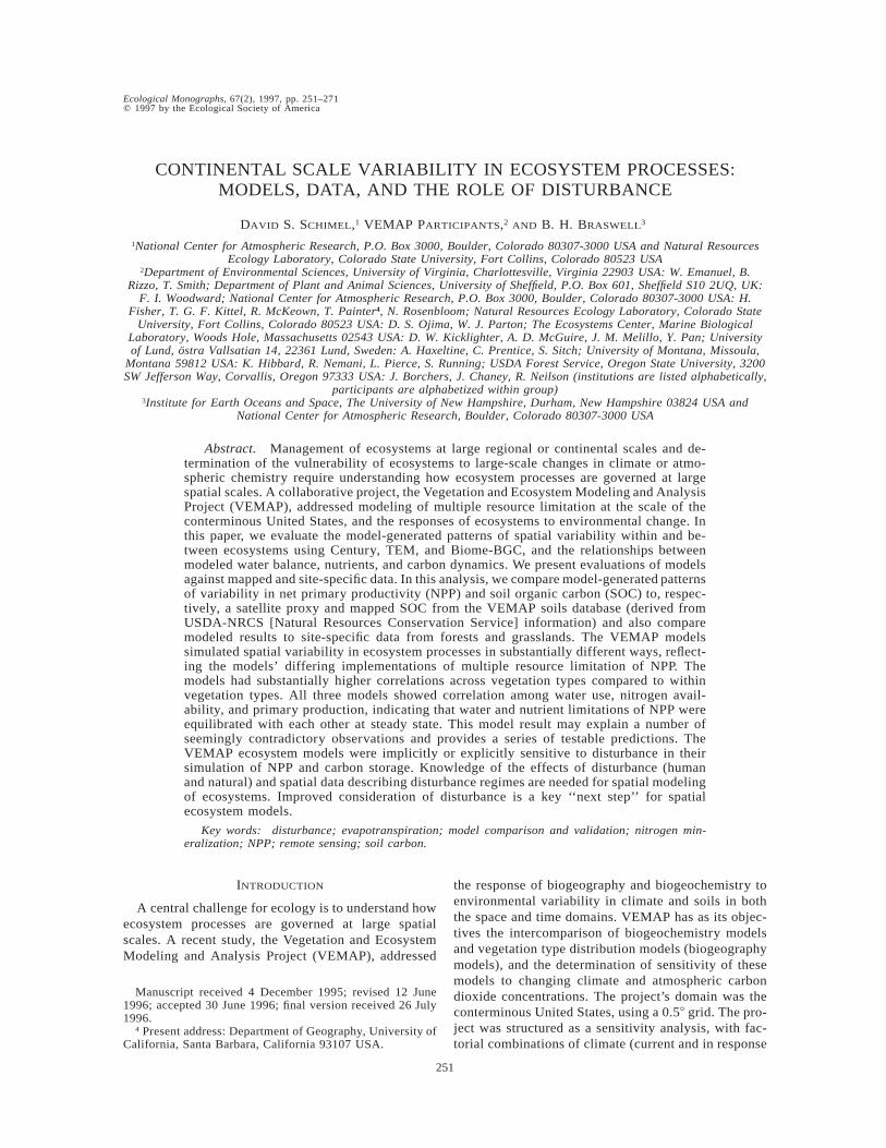
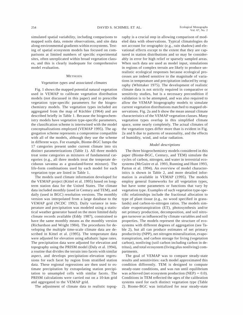
Fig. 1. Map of the vegetation classes used in VEMAP (see Table 1 for additional description). ‘‘Xerowoods’’ indicates thexeromorphic woodland category. Wetland classes were not included in model calculations.

←

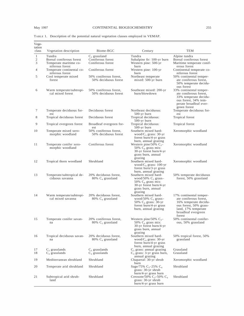
Fig. 2. Box-plots for (a) mean annual temperature and (b) mean annual precipitation. The white bar within each boxmarks the mean value, the upper and lower edges of the box mark the first and third quartiles, the upper and lower bracketsdenote the 95th and 5th percentiles, and the black dashes indicate outliers for each vegetation type. Red arrows on Fig. 2aand b indicate the mean annual temperature and precipitation of OTTER experiment sites within the maritime coniferousvegetation type (Runyon et al. 1994), and of the Konza and CPER LTER sites within the C4 grasslands.

to projected doubled CO2), atmospheric CO2, andmapped and model-generated vegetation distributions.Maps of climate, climate change scenarios, soil prop-erties, and potential natural vegetation were preparedas common inputs to the models (Kittel et al. 1995) toallow for rigorous intercomparison. VEMAP (1995)compared the models’ spatially aggregated responsesin the simulation of contemporary conditions and sen-sitivity to change. That paper also drew preliminaryconclusions regarding links between the model-specificresponses in the sensitivity analysis and the mecha-nisms and parameter values employed in those models.Initial analyses from VEMAP suggested that model-specific differences in sensitivity to changes in physicalvariables vs. internal nutrient limitations caused dif-ferences in modeled sensitivity to climate change (VE-MAP 1995). This paper extends that analysis usingspatial variability along environmental gradients underthe current climate to better understand the complexresponses of the VEMAP biogeochemistry models tothe physical environment and nutrient cycling.

Because many environmental changes imply changesto environmental resources through changing climate,atmospheric nutrient deposition, and species compo-sition, understanding the interactions of environmentalresources is a precondition for credible predictive mod-eling (Ehleringer and Field 1993). Environmental re-sources (light, water, nutrients) and plant attributes(e.g., carbon and nitrogen status and allocation, tissuechemistry) are linked to production and decomposition(Farqhuar et al. 1980, Melillo et al. 1984, Bloom et al.1985, Chapin et al. 1987, Nobel 1991, Running andNemani 1991). The concepts of multiple resource lim-itation have been explored in theoretical and empiricalstudies (Thornley 1972, Bloom et al. 1985, Tilman1985, Ingestad and Lund 1986, Chapin et al. 1987,Field 1991, Schimel et al. 1991). Joint limitation bycarbon dioxide, water, light, and nitrogen affects plantgrowth, allocation patterns, nutrient cycling, and com-petition (Christie and Detling 1982, Eisele et al. 1989,Wedin and Tilman 1990, Schimel et al. 1991).

Spatial models based on multiple resource limitationrequire information describing spatial–temporal pat-terns of resource distribution and availability. Earlyefforts to link ecological responses to environmentalgradients included only variables related to temperature

and precipitation (e.g., Holdridge 1967, Lieth 1972,Esser 1986). Current spatial models of productivity,carbon storage, and nutrient cycling, ‘‘biogeochemistrymodels,’’ use additional information on climate (ra-diation, humidity, and other sources) and soil proper-ties, and include vegetation type-specific parameters(Burke et al. 1991, Burke and Lauenroth 1993, Mc-Guire et al. 1993, Running and Hunt 1993, Schimel etal. 1994, VEMAP 1995). These models simulate thecomponents of spatial variability in ecosystem pro-cesses governed by climate, soil, and vegetation type.As a result they use, and require, maps of these vari-ables as input (Kittel et al. 1995).

The biogeochemistry models employed in VEMAPall include multiple environmental resources (water,light, nutrients) as controls over plant and ecosystemprocesses, although with quite different approaches(TEM: McGuire et al. 1993; Biome-BGC: Running andHunt 1993; Century: Parton et al. 1994, Schimel et al.1994). VEMAP (1995) identified differences in rep-resentation of multiple resource limitation as one ofthe most important factors controlling the models’ ag-gregate responses to environmental change. The inter-action of the spatial distribution of environmental re-sources, or controls over resource availability (e.g., soilproperties), with model-specific mechanisms will in-fluence spatial patterns of ecosystem response to mul-tiple environmental resources and stresses.

This paper is a follow on and expansion of the VE-MAP (1995) work, analyzing the responses of the bio-geochemistry models under current climate and currentCO2 concentrations. The objectives of this paper weretwofold: to utilize spatial variability in model responsesto diagnose the importance of different underlyingmechanisms, and to explore methodology and data setsfor evaluating simulated spatial variability relative toobservations. For the first objective we utilized the spa-tial gradients of environmental resources within theVEMAP domain to quantify differences in sensitivityto climatic vs. biogeochemical processes between themodels. Such differences in sensitivity were hypoth-esized to result in the different responses to alteredclimate and CO2 among TEM, Century, and Biome-BGC (VEMAP 1995); this paper provides quantitativeevaluation of intermodel differences. Second, we ex-plored a variety of approaches to testing the fidelity of


simulated spatial variability, including comparisons tomapped soils data, remote observations, and site dataalong environmental gradients within ecosystems. Test-ing of spatial ecosystem models has focused on com-parisons at limited numbers of specific experimentalsites, often unreplicated within broad vegetation class-es, and this is clearly inadequate for comprehensivemodel evaluation.

METHODS

Vegetation types and associated climates

Fig. 1 shows the mapped potential natural vegetationused in VEMAP to calibrate vegetation distributionmodels (not discussed in this paper) and to prescribevegetation type-specific parameters for the biogeo-chemistry models. The vegetation types included areaggregated from the map of Kuchler (1964) and aredescribed briefly in Table 1. Because the biogeochem-istry models have vegetation type-specific parameters,the classification scheme is intertwined with the modelconceptualizations employed (VEMAP 1995). The ag-gregation scheme represents a compromise compatiblewith all of the models, although they use the schemein different ways. For example, Biome-BGC lumps the17 categories present under current climate into sixdistinct parameterizations (Table 1). All three modelstreat some categories as mixtures of fundamental cat-egories (e.g., all three models treat the temperate de-ciduous savanna as a grassland/forest mixture). Thelife-form combinations used by each model for eachvegetation type are listed in Table 1.

The models used climate information developed forthe VEMAP project (Kittel et al. 1995) based on long-term station data for the United States. The climatedata included monthly (used in Century and TEM), anddaily (used in BGC) resolution versions. The monthlyversion was interpolated from a large database to theVEMAP grid (NCDC 1992). Daily variance in tem-perature and precipitation was modeled using a statis-tical weather generator based on the more limited dailyclimate records available (Eddy 1987), constrained tohave the same monthly means as the monthly version(Richardson and Wright 1984). The procedures for de-veloping the multiple time-scale climate data are de-scribed in Kittel et al. (1995). The temperature datawere adjusted for elevation using adiabatic lapse rates.The precipitation data were adjusted for elevation andtopography using the PRISM model (Daly et al. 1994),a routine that divides the terrain into facets with similaraspect, and develops precipitation–elevation regres-sions for each facet by region from stratified stationdata. These regional regressions are then used to es-timate precipitation by extrapolating station precipi-tation to unsampled cells with similar facets. ThePRISM calculations were carried out on a 10-km gridand aggregated to the VEMAP grid.

The adjustment of climate data to realistic topog-

raphy is a crucial step in allowing comparison of mod-eled data with observations. Typical climatologies donot account for orographic (e.g., rain shadow) and ele-vational effects except to the extent that they are cap-tured in station distributions and so may be consider-ably in error for high relief or sparsely sampled areas.When such data are used as model input, simulationsin regions of complex terrain are likely to produce un-realistic ecological responses because ecological pro-cesses are indeed sensitive to the magnitude of varia-tions in temperature and precipitation induced by orog-raphy (Whittaker 1975). The development of realisticclimate data is not strictly required in comparative orsensitivity studies, but is a necessary precondition ifvalidation is to be attempted, and was also required toallow the VEMAP biogeography models to simulatecurrent vegetation distributions matched to mapped ob-servations. Fig. 2a and b show the mean annual climatecharacteristics of the VEMAP vegetation classes. Manyvegetation types overlap in this simplified climatespace, some nearly completely. The actual climates ofthe vegetation types differ more than is evident in Fig.2a and b due to patterns of seasonality, and the effectsof humidity, wind, and solar radiation.

Model descriptions

The three biogeochemistry models considered in thispaper (Biome-BGC, Century, and TEM) simulate thecycles of carbon, nitrogen, and water in terrestrial eco-systems (McGuire et al. 1993, Running and Hunt 1993,Parton et al. 1994). An overview of model character-istics is shown in Table 2, and more detailed infor-mation is available in VEMAP (1995). The modelsemploy general frameworks for all vegetation types,but have some parameters or functions that vary byvegetation type. Examples of such vegetation type-spe-cific relationships include the fractional allocation totype of plant tissue (e.g., no wood specified in grass-lands) and carbon-to-nitrogen ratios. The models sim-ulate evapotranspiration (ET), photosynthesis and/ornet primary production, decomposition, and soil nitro-gen turnover as influenced by climate variables and soilproperties. The models represent the structure of eco-systems with different degrees of aggregation (see Ta-ble 2), but all can produce estimates of net primaryproductivity (NPP), net nitrogen mineralization, evapo-transpiration, and carbon storage for living (vegetationcarbon), nonliving (soil carbon including carbon in de-tritus), and total ecosystem (living plus nonliving) com-partments.

The goal of VEMAP was to compare steady-stateresults and sensitivities: each model approximated thiscondition differently. TEM is designed to computesteady-state conditions, and was run until equilibriumwas achieved (net ecosystem production (NEP) 5 0.0).Conditions in TEM reflected the ages of the calibrationsystems used for each distinct vegetation type (Table2). Biome-BGC was initialized for near steady-state


TABLE 1. Description of the potential natural vegetation classes employed in VEMAP.

Vege-tationclass Vegetation description Biome-BGC Century TEM

1 Tundra C3 grassland Tundra Alpine tundra2 Boreal coniferous forest Coniferous forest Subalpine fir: 100-yr burn Boreal coniferous forest3 Temperate maritime co-

niferous forestConiferous forest Western pine: 500-yr

burnMaritime temperate conif-

erous forest4 Temperate continental co-

niferous forestConiferous forest Western pine: 100-yr

burnContinental temperate co-

niferous forest5 Cool temperate mixed

forest50% coniferous forest,

50% deciduous forestNortheast temperate

mixed: 500-yr burn50% continental temper-

ate coniferous forest,50% temperate decidu-ous forest

6 Warm temperate/subtropi-cal mixed forest

50% coniferous forest,50% deciduous forest

Southeast mixed: 200-yrburn/blowdown

33% continental temper-ate coniferous forest,33% temperate decidu-ous forest, 34% tem-perate broadleaf ever-green forest

7 Temperate deciduous for-est

Deciduous forest Northeast deciduous:500-yr burn

Temperate deciduous for-est

8 Tropical deciduous forest Deciduous forest Tropical deciduous:500-yr burn

Tropical forest

9 Tropical evergreen forest Broadleaf evergreen for-est

Tropical deciduous:500-yr burn

Tropical forest

10 Temperate mixed xero-morphic woodland

50% coniferous forest,50% deciduous forest

Southern mixed hard-wood/C3 grass: 30-yrforest burn/4-yr grassburn, annual grazing

Xeromorphic woodland

11 Temperate conifer xero-morphic woodland

Coniferous forest Western pine/50% C3–50% C4 grass mix:30-yr forest burn/4-yrgrass burn, annualgrazing


12 Tropical thorn woodland Shrubland Southern mixed hard-wood/C4 grass: 100-yrforest burn/3-yr grassburn, annual grazing


13 Temperate/subtropical de-ciduous savanna

20% deciduous forest,80% C4 grassland

Southern mixed hard-wood/50% C3 grass–50% C4 grass mix:30-yr forest burn/4-yrgrass burn, annualgrazing

50% temperate deciduousforest, 50% grassland

14 Warm temperate/subtropi-cal mixed savanna


Southern mixed hard-wood/50% C3 grass–50% C4 grass: 30-yrforest burn/4-yr grassburn, annual grazing

17% continental temper-ate coniferous forest,16% temperate decidu-ous forest, 50% grass-land, 17% temperatebroadleaf evergreenforest

15 Temperate conifer savan-na

20% coniferous forest,80% C3 grassland

Western pine/50% C3–50% C4 grass mix:30-yr forest burn/4-yrgrass burn, annualgrazing

50% continental conifer-ous, 50% grassland

16 Tropical deciduous savan-na


Southern mixed hard-wood/C4 grass: 30-yrforest burn/4-yr grassburn, annual grazing

50% tropical forest, 50%grassland

17 C3 grasslands C3 grasslands C3 grass: annual grazing Grassland18 C4 grasslands C4 grasslands C4 grass: 3-yr grass burn,

annual grazingGrassland

19 Mediterranean shrubland Shrubland Chaparral: 30-yr shrubburn


20 Temperate arid shrubland Shrubland Sage/75% C3–25% C4

grass: 30-yr shrubburn/4-yr grass burn

Shrubland

21 Subtropical arid shrub-land

Shrubland Creosote/50% C3–50% C4

grass: 30-yr shrubburn/4-yr grass burn

Shrubland


TABLE 2. Comparison of biogeochemical and physiological processes, and compartments among the biogeochemistry modelsemployed in VEMAP.

Process Biome-BGC Century TEM

Temporal scale Daily/annual Monthly MonthlyEquilibrium Carbon pools specified so

NEP 5 0 after 1 yrSimulation with repeated

disturbance for 2000 yrDynamic simulation (10–

3000 yr) until C and Npools balance (e.g., N in-put 5 N loss)

Potential evapotranspiration(PET)/evapotranspiration(ET)

Penman-Monteith Modified Penman-Monteith Jensen-Haise (1963)

Number of soil water layers 1 5 1Number of vegetation carbon

pools4 8 1

Number of litter/soil carbonpools

3 13 1

Number of vegetation nitrogenpools

4 8 2

Number of litter/soil nitrogenpools

3 15 2

Leaf Area Index (LAI) Water balance†, N availabil-ity and gross photosynthe-sis

Leaf biomass Not explicitly calculated

Plant respiration Q10 2.0 2.0 1.5–2.5Decomposition Q10 2.4 ;2.0 2.0Stomatal conductance 5 f(Ca) Yes Implicitly NoCi 5 f(Ca) Yes Not applicable YesVegetation C/N 5 f(Ca) Yes Yes NoCarbon uptake by vegetation Farquhar Multiple limitation NPP Multiple limitation GPPNitrogen uptake by vegetation Annual Monthly MonthlyNet nitrogen mineralization

(Nmin)C/N ratio controlled Multiple compartment miner-

alization/immobilizationMineralization/immobiliza-

tion dynamics

† For the VEMAP activity, LAI is a function of water balance only; Ca is atmospheric concentration; Ci is internal CO2

concentration within a ‘‘leaf’’; NPP is net primary production; GPP is gross primary production.

conditions, using allometric relationships, but then, be-cause of computing constraints run for just one year.(Biome-BGC, uses a daily time step and required morecomputer time to run to steady state for the entire VE-MAP grid than was available to Running and collab-orators; S. W. Running, personal communication.) Cen-tury was run to steady state for grasslands. For forests,Century does not achieve a steady-state condition. In-stead, forest results were reported at the ages corre-sponding to the age of TEM’s calibration stands, agesthat varied by vegetation type (Table 2). Century forestresults may have nonzero NEP, thereby differing fromthe other two models. Thus, all three models requirean implicit or explicit assumed stand age linking thisstudy to knowledge of, and assumptions about, forestdemography at large scales (see Table 1).

Experimental protocol

The entire VEMAP experimental protocol was fac-torial, including effects of climate change, increasingatmospheric CO2, and redistribution of vegetation types(VEMAP 1995, Kittel et al. 1995). In this paper, weconsider only simulations using current climate, cur-rent atmospheric CO2 (354 mL/L), and potential naturalvegetation derived from Kuchler (1964). The modelswere run using a common spatial format (0.5 3 0.58grid) containing 3261 land grid cells. Climate, soil, andvegetation data, along with climate change scenarios,are available; see Acknowledgments.

Required soil properties (depth, water holding ca-pacity, and texture: percentage sand, silt, clay) werebased on Kern’s (1994, 1995) 10-km gridded UnitedStates Natural Resource Conservation Service database (NATSCO). Soil carbon was also gridded fromKern’s (1994) data base as a validation variable. Weused cluster analysis to group the 10-km soil units intoone to four ‘‘modes’’ within each grid cell. Soils withinclusters have quantitatively similar (in a multivariatesense) soil properties. We averaged soil propertieswithin the areally dominant mode, thus averaging theproperties of generally similar soils, and assigned thoseproperties to the cell. This avoided two problems, thefirst being the threat of averaging diverse soils to yielda type that might not actually occur in the grid cell(e.g., sand averaged with clay to yield a loam). In ourapproach soils within clusters can differ by a few per-cent in texture or organic matter but never by 10–20%;i.e., not by the differences between major texture class-es. The second problem we avoided was in diverseregions where the single most common soil type mightcompose a plurality (rather than the majority) of thecell. Using our algorithm, we average soil propertieswithin the areally dominant mode, thereby averagingquantitatively similar soils together. Thus the single,areally dominant soil could be a sandy type, but themajority of the grid cell could be an array of clayeysoils ranging in texture from 28 to 35% clay. In ouralgorithm these clay soils would be aggregated together


to assign the average texture for the cell instead ofusing the areally dominant sandy soil.

Satellite data

Data from the NASA/NOAA Pathfinder Programwere used to produce satellite vegetation indices foruse in model evaluation. The Pathfinder land data set(see Acknowledgments) is derived from measurementsmade by the Advanced Very High Resolution Radi-ometer (AVHRR) on board the NOAA TIROS-N seriesof polar orbiting satellites. The optical data are cali-brated for reflectance. The data are projected onto an8 3 8 km equal-area grid and temporally compositedto scenes within 10-d windows from the original dailydata. The Pathfinder processing also includes cloudscreening and partial atmospheric correction (for ozoneand Raleigh scattering). The normalized differencevegetation index (NDVI) can be computed from thetwo AVHRR optical channels (Tucker 1979, Gowardet al. 1991).

There have been many studies that relate the NDVIto ecological quantities at local, regional, and globalscales (Asrar et al. 1984, Fung et al. 1987). Most rel-evant for this study, the growing season integral of theNDVI is related to terrestrial net primary productivity(Goward et al. 1985) based on good empirical corre-lations and a strong theoretical basis (Goward et al.1985, Sellers 1985, Fung et al. 1987, Schimel et al.1991, Potter et al. 1993). Although there is uncertaintyinvolved in calculating NPP from the NDVI becauseof atmospheric and geometric bidirectional effects andvegetation type-specific relationships, it is robust as aproxy. Also, by recompositing and averaging, we min-imized these effects. NDVI has the important advan-tage of being an actual measurement made everywherein the study domain, rather than being interpolated orextrapolated to a map, as is mapped soil organic carbon(SOC) (Schimel and Potter 1995).

We produced a data set that is the annual integral ofNDVI (iNDVI) averaged over the 3 yr of Pathfinderdata available at the time of this study (1986–1988).We first extracted the continental United States fromthe global grid and recomposited the data to monthlyscenes by choosing the greenest pixels (an additionaland conservative technique for minimizing cloud andsun/sensor angular geometry effects). The monthly val-ues were then averaged for each pixel, and the twelveresulting maps reprojected to the VEMAP 0.5 3 0.58grid. The iNDVI values were then divided by 12 toretain the familiar [21, 1] range for NDVI.

Data analysis

In order to separate continental and within-vegeta-tion type variations and to identify patterns of agree-ment and disagreement between models on a grid cell-to-grid cell level, we carried out a simple data trans-formation. We computed the ‘‘mean deviates’’ of grid-ded values for each variable and model to create a

transformed variable by subtracting the mean from eachvalue. For our analyses, the transformation was suchthat for each variable X in each grid cell (i, j) in eachvegetation class V, the mean deviate of XV(i, j) was:

MDV(i, j) 5 Xv(i, j) 2 Xv (1)

where Xv is the mean for variable X within vegetationclass V. Transformed variables XV included outputssuch as NPP, total carbon storage, and evapotranspi-ration, and inputs such as annual precipitation or soilclay content. We also computed the mean deviates ofthe iNDVI and mapped SOC as model evaluation vari-ables. By subtracting the mean, we eliminated model-to-model bias in the mean, and the large between-veg-etation type differences in model results. We subtractthe vegetation type-specific means (rather than the con-tinental average) because the models use different par-ameterizations for the different vegetation types, andso the biases and type-to-type effects are type specific.The mean deviates allow us to examine patterns inspatial variability within vegetation types, but in thecontinental aggregate.

RESULTS

Analysis of mean deviates

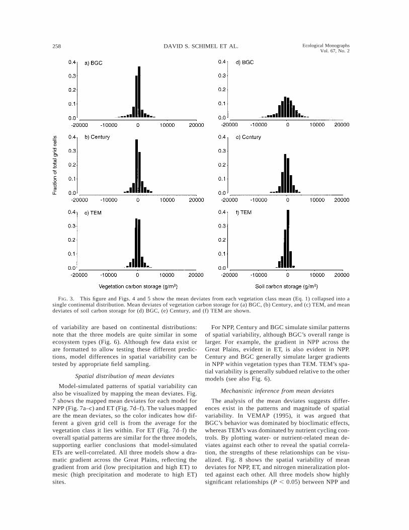
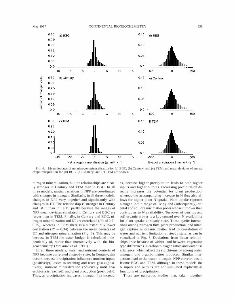
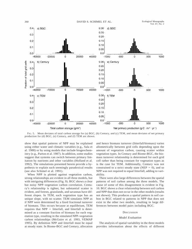
Mean deviates of the original data were used to vi-sualize the degree of spatial variability within vege-tation types for each model. We then collapsed themean deviates into continental-scale distributions, asdisplayed in Figs. 3, 4, and 5. Analysis of the meandeviates shows different patterns of variability for bothdifferent models and different variables. In all threemodels, the mean deviates of vegetation carbon aresmall (Fig. 3a–c), likely because of the assumption ofa uniform stand age (explicitly, as in Century, implic-itly in TEM and BGC). Soil carbon shows quite a dif-ferent pattern, with a wide range of mean deviates forBGC, a narrow range for TEM, and Century inter-mediate (Fig. 3d–f). The mean deviates for nitrogenmineralization and evapotranspiration are similaracross models (Fig. 4a–f). Total carbon and NPP showpatterns similar to soil carbon, with broad, interme-diate, and narrow ranges of mean deviates for BGC,Century, and TEM, respectively (Fig. 5a–f).

BGC consistently simulated large variations in eco-system processes within vegetation types and TEMsimulated small variations. Century is intermediate inits simulation of spatial variability. We cannot assessrigorously which, if any, simulated patterns of spatialvariability are correct, but this analysis provides a foun-dation for additional data analysis or collection neededin model validation. TEM’s generally low spatial vari-ability is consistent with a view that at the VEMAPgrid scale, typical high stand-to-stand variability av-erages out. By contrast, Biome-BGC preserved the lev-el of variability typical of hectare-to-hectare variabilityin field studies at the VEMAP grid scale. These patterns


FIG. 3. This figure and Figs. 4 and 5 show the mean deviates from each vegetation class mean (Eq. 1) collapsed into asingle continental distribution. Mean deviates of vegetation carbon storage for (a) BGC, (b) Century, and (c) TEM, and meandeviates of soil carbon storage for (d) BGC, (e) Century, and (f) TEM are shown.

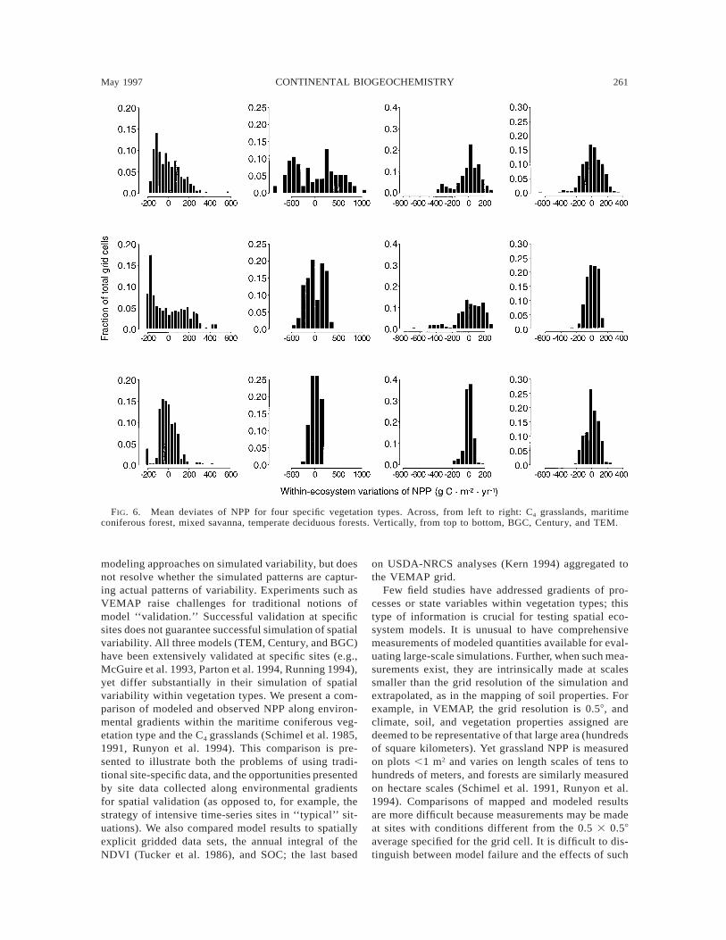
of variability are based on continental distributions:note that the three models are quite similar in someecosystem types (Fig. 6). Although few data exist orare formatted to allow testing these different predic-tions, model differences in spatial variability can betested by appropriate field sampling.

Spatial distribution of mean deviates

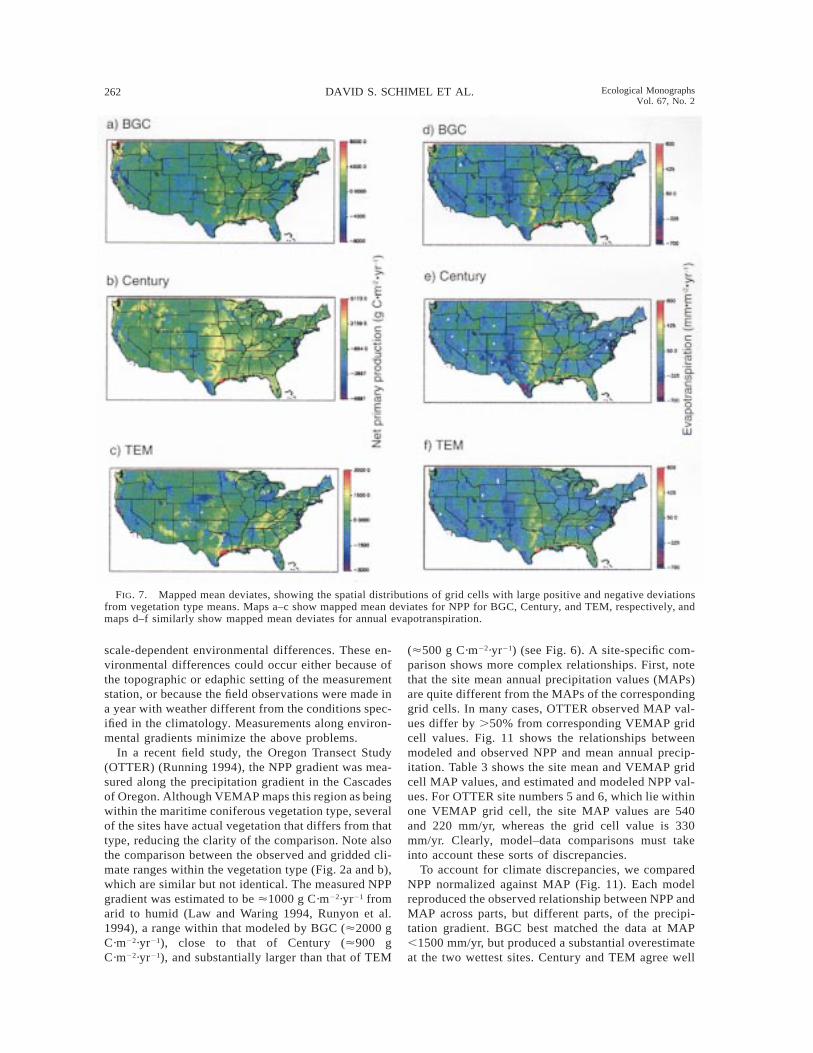
Model-simulated patterns of spatial variability canalso be visualized by mapping the mean deviates. Fig.7 shows the mapped mean deviates for each model forNPP (Fig. 7a–c) and ET (Fig. 7d–f). The values mappedare the mean deviates, so the color indicates how dif-ferent a given grid cell is from the average for thevegetation class it lies within. For ET (Fig. 7d–f) theoverall spatial patterns are similar for the three models,supporting earlier conclusions that model-simulatedETs are well-correlated. All three models show a dra-matic gradient across the Great Plains, reflecting thegradient from arid (low precipitation and high ET) tomesic (high precipitation and moderate to high ET)sites.

For NPP, Century and BGC simulate similar patternsof spatial variability, although BGC’s overall range islarger. For example, the gradient in NPP across theGreat Plains, evident in ET, is also evident in NPP.Century and BGC generally simulate larger gradientsin NPP within vegetation types than TEM. TEM’s spa-tial variability is generally subdued relative to the othermodels (see also Fig. 6).

Mechanistic inference from mean deviates

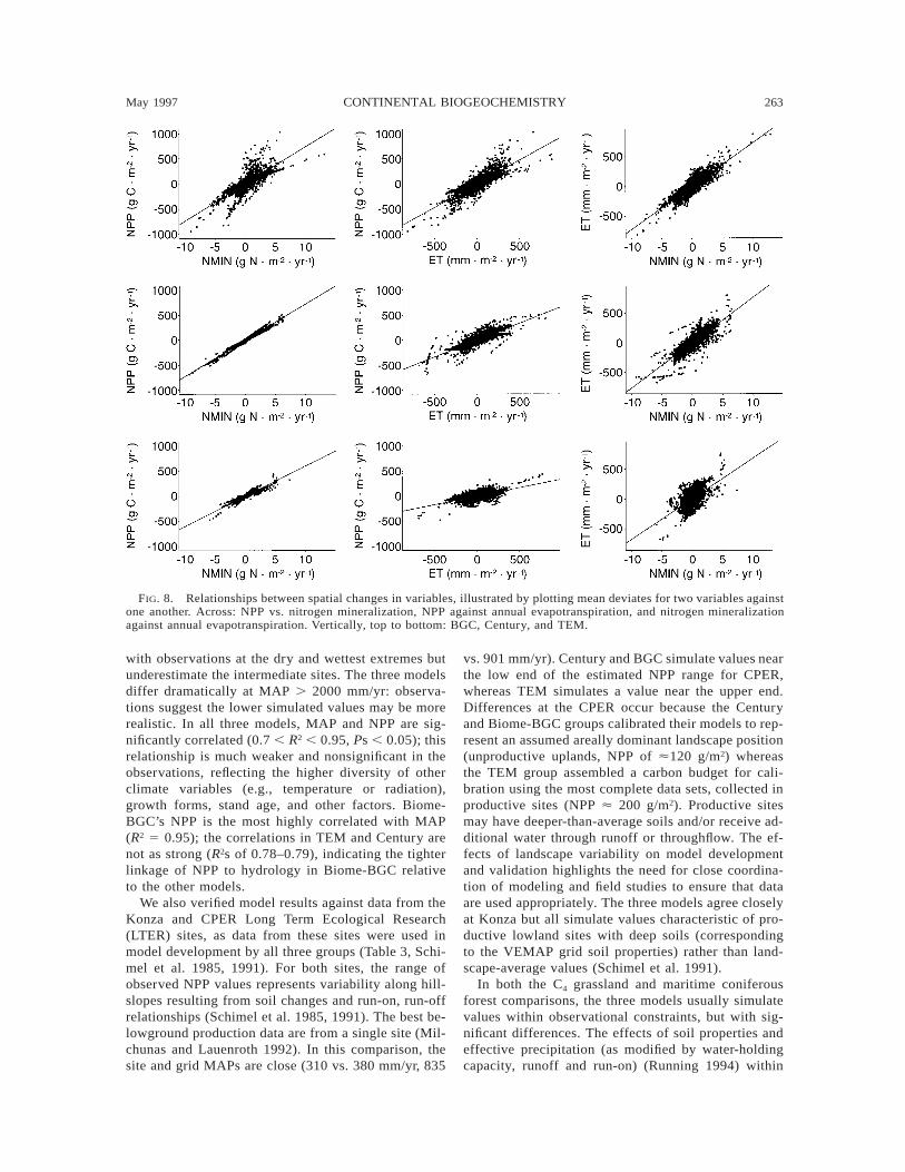
The analysis of the mean deviates suggests differ-ences exist in the patterns and magnitude of spatialvariability. In VEMAP (1995), it was argued thatBGC’s behavior was dominated by bioclimatic effects,whereas TEM’s was dominated by nutrient cycling con-trols. By plotting water- or nutrient-related mean de-viates against each other to reveal the spatial correla-tion, the strengths of these relationships can be visu-alized. Fig. 8 shows the spatial variability of meandeviates for NPP, ET, and nitrogen mineralization plot-ted against each other. All three models show highlysignificant relationships (P , 0.05) between NPP and


FIG. 4. Mean deviates of net nitrogen mineralization for (a) BGC, (b) Century, and (c) TEM, and mean deviates of annualevapotranspiration for (d) BGC, (e) Century, and (f) TEM are shown.

nitrogen mineralization, but the relationships are clear-ly stronger in Century and TEM than in BGC. In allthree models, spatial variations in NPP are coordinatedwith changes in nitrogen. Similarly, in all three models,changes in NPP vary together and significantly withchanges in ET. The relationship is stronger in Centuryand BGC than in TEM, partly because the ranges ofNPP mean deviates simulated in Century and BGC arelarger than in TEM. Finally, in Century and BGC, ni-trogen mineralization and ET are correlated (R2s of 0.7–0.75), whereas in TEM there is a substantially lowercorrelation (R2 5 0.34) between the mean deviates ofET and nitrogen mineralization (Fig. 8). This may bebecause in TEM the water budget is calculated inde-pendently of, rather than interactively with, the bio-geochemistry (McGuire et al. 1993).

In all three models, water and nutrient controls ofNPP become correlated at steady state. In Century, thisoccurs because precipitation influences nutrient inputs(positively), losses to leaching and trace gases (posi-tively), nutrient mineralization (positively until ana-erobiosis is reached), and plant production (positively).Thus, as precipitation increases, nitrogen flux increas-

es, because higher precipitation leads to both higherinputs and higher outputs. Increasing precipitation di-rectly increases the potential for plant production,whereas the accompanying increase in N flux also al-lows for higher plant N uptake. Plant uptake capturesnitrogen into a range of living and (subsequently) de-trital and soil organic matter pools whose turnover thencontributes to N availability. Turnover of detritus andsoil organic matter is a key control over N availabilityfor plant uptake at steady state. These cyclic interac-tions among nitrogen flux, plant production, and nitro-gen capture in organic matter lead to correlation ofwater and nutrient limitation at steady state, as can bevisualized in Fig. 8. Deviations from linear relation-ships arise because of within- and between-vegetationtype differences in carbon:nitrogen ratios and water useefficiency, which affect the stoichiometry among water,nitrogen, and organic matter produced. Similar inter-actions lead to the water–nitrogen–NPP correlations inBiome-BGC and TEM, although in these models theN inputs and outputs are not simulated explicitly asfunctions of precipitation.

There are numerous studies that, taken together,


FIG. 5. Mean deviates of total carbon storage for (a) BGC, (b) Century, and (c) TEM, and mean deviates of net primaryproduction for (d) BGC, (e) Century, and (f) TEM are shown.

show that spatial patterns of NPP may be explainedusing either water and climatic variables (e.g., Sala etal. 1988) or by using models that include biogeochem-istry (e.g., Parton et al. 1987). In addition, some studiessuggest that systems can switch between primary lim-itation by nutrients and other variables (Holland et al.1992). The simulations presented herein provide a hy-pothesis to explain such seemingly paradoxical results(see also Schimel et al. 1991).

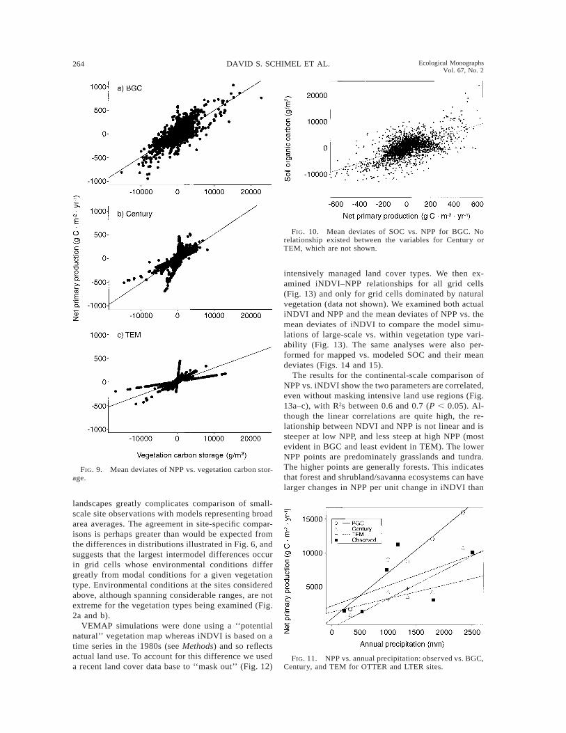
When NPP is plotted against vegetation carbon,strong relationships are evident in all three models, butwith intriguing differences (Fig. 9). BGC shows a clearbut noisy NPP–vegetation carbon correlation. Centu-ry’s relationship is tighter, but substantial scatter isevident, and forests, grasslands, and savannas have dif-ferent slopes. In TEM, each vegetation type has anunique slope, with no scatter. TEM simulates NPP asif NPP were determined by a fixed fractional turnoverof biomass. This occurs because at equilibrium, TEMrequires that NPP 5 litterfall, and litterfall is deter-mined as a constant fraction of biomass for each veg-etation type, resulting in the simulated NPP–vegetationcarbon relationships (McGuire et al. 1993, VEMAP1995). By definition NPP and litterfall must be equalat steady state. In Biome-BGC and Century, allocation

and hence biomass turnover (litterfall/biomass) variesallometrically between grid cells depending upon theamount of vegetation carbon, causing scatter withinvegetation types. In Century and Biome-BGC, the bio-mass turnover relationship is determined for each gridcell rather than being constant for vegetation types asis the case for TEM. Additionally, Century was notconstrained to a strict steady state (NEP 5 0), and soNPP was not required to equal litterfall, adding to vari-ability.

There were also large differences between the spatialpatterns of soil carbon among the three models. Thecause of some of this disagreement is evident in Fig.10. BGC shows a clear relationship between soil carbonand NPP that does not occur in the other models (resultsnot shown). This produces a spatial pattern in soil car-bon in BGC related to patterns in NPP that does notexist in the other two models, resulting in large dif-ferences between model pairs including BGC.

DISCUSSION

Model Evaluation

The analysis of spatial variability in the three modelsprovides information about the effects of different


FIG. 6. Mean deviates of NPP for four specific vegetation types. Across, from left to right: C4 grasslands, maritimeconiferous forest, mixed savanna, temperate deciduous forests. Vertically, from top to bottom, BGC, Century, and TEM.

modeling approaches on simulated variability, but doesnot resolve whether the simulated patterns are captur-ing actual patterns of variability. Experiments such asVEMAP raise challenges for traditional notions ofmodel ‘‘validation.’’ Successful validation at specificsites does not guarantee successful simulation of spatialvariability. All three models (TEM, Century, and BGC)have been extensively validated at specific sites (e.g.,McGuire et al. 1993, Parton et al. 1994, Running 1994),yet differ substantially in their simulation of spatialvariability within vegetation types. We present a com-parison of modeled and observed NPP along environ-mental gradients within the maritime coniferous veg-etation type and the C4 grasslands (Schimel et al. 1985,1991, Runyon et al. 1994). This comparison is pre-sented to illustrate both the problems of using tradi-tional site-specific data, and the opportunities presentedby site data collected along environmental gradientsfor spatial validation (as opposed to, for example, thestrategy of intensive time-series sites in ‘‘typical’’ sit-uations). We also compared model results to spatiallyexplicit gridded data sets, the annual integral of theNDVI (Tucker et al. 1986), and SOC; the last based

on USDA-NRCS analyses (Kern 1994) aggregated tothe VEMAP grid.

Few field studies have addressed gradients of pro-cesses or state variables within vegetation types; thistype of information is crucial for testing spatial eco-system models. It is unusual to have comprehensivemeasurements of modeled quantities available for eval-uating large-scale simulations. Further, when such mea-surements exist, they are intrinsically made at scalessmaller than the grid resolution of the simulation andextrapolated, as in the mapping of soil properties. Forexample, in VEMAP, the grid resolution is 0.58, andclimate, soil, and vegetation properties assigned aredeemed to be representative of that large area (hundredsof square kilometers). Yet grassland NPP is measuredon plots ,1 m2 and varies on length scales of tens tohundreds of meters, and forests are similarly measuredon hectare scales (Schimel et al. 1991, Runyon et al.1994). Comparisons of mapped and modeled resultsare more difficult because measurements may be madeat sites with conditions different from the 0.5 3 0.58average specified for the grid cell. It is difficult to dis-tinguish between model failure and the effects of such


FIG. 7. Mapped mean deviates, showing the spatial distributions of grid cells with large positive and negative deviationsfrom vegetation type means. Maps a–c show mapped mean deviates for NPP for BGC, Century, and TEM, respectively, andmaps d–f similarly show mapped mean deviates for annual evapotranspiration.

scale-dependent environmental differences. These en-vironmental differences could occur either because ofthe topographic or edaphic setting of the measurementstation, or because the field observations were made ina year with weather different from the conditions spec-ified in the climatology. Measurements along environ-mental gradients minimize the above problems.

In a recent field study, the Oregon Transect Study(OTTER) (Running 1994), the NPP gradient was mea-sured along the precipitation gradient in the Cascadesof Oregon. Although VEMAP maps this region as beingwithin the maritime coniferous vegetation type, severalof the sites have actual vegetation that differs from thattype, reducing the clarity of the comparison. Note alsothe comparison between the observed and gridded cli-mate ranges within the vegetation type (Fig. 2a and b),which are similar but not identical. The measured NPPgradient was estimated to be ø1000 g C·m22·yr21 fromarid to humid (Law and Waring 1994, Runyon et al.1994), a range within that modeled by BGC (ø2000 gC·m22·yr21), close to that of Century (ø900 gC·m22·yr21), and substantially larger than that of TEM

(ø500 g C·m22·yr21) (see Fig. 6). A site-specific com-parison shows more complex relationships. First, notethat the site mean annual precipitation values (MAPs)are quite different from the MAPs of the correspondinggrid cells. In many cases, OTTER observed MAP val-ues differ by .50% from corresponding VEMAP gridcell values. Fig. 11 shows the relationships betweenmodeled and observed NPP and mean annual precip-itation. Table 3 shows the site mean and VEMAP gridcell MAP values, and estimated and modeled NPP val-ues. For OTTER site numbers 5 and 6, which lie withinone VEMAP grid cell, the site MAP values are 540and 220 mm/yr, whereas the grid cell value is 330mm/yr. Clearly, model–data comparisons must takeinto account these sorts of discrepancies.

To account for climate discrepancies, we comparedNPP normalized against MAP (Fig. 11). Each modelreproduced the observed relationship between NPP andMAP across parts, but different parts, of the precipi-tation gradient. BGC best matched the data at MAP,1500 mm/yr, but produced a substantial overestimateat the two wettest sites. Century and TEM agree well


FIG. 8. Relationships between spatial changes in variables, illustrated by plotting mean deviates for two variables againstone another. Across: NPP vs. nitrogen mineralization, NPP against annual evapotranspiration, and nitrogen mineralizationagainst annual evapotranspiration. Vertically, top to bottom: BGC, Century, and TEM.

with observations at the dry and wettest extremes butunderestimate the intermediate sites. The three modelsdiffer dramatically at MAP . 2000 mm/yr: observa-tions suggest the lower simulated values may be morerealistic. In all three models, MAP and NPP are sig-nificantly correlated (0.7 , R2 , 0.95, Ps , 0.05); thisrelationship is much weaker and nonsignificant in theobservations, reflecting the higher diversity of otherclimate variables (e.g., temperature or radiation),growth forms, stand age, and other factors. Biome-BGC’s NPP is the most highly correlated with MAP(R2 5 0.95); the correlations in TEM and Century arenot as strong (R2s of 0.78–0.79), indicating the tighterlinkage of NPP to hydrology in Biome-BGC relativeto the other models.

We also verified model results against data from theKonza and CPER Long Term Ecological Research(LTER) sites, as data from these sites were used inmodel development by all three groups (Table 3, Schi-mel et al. 1985, 1991). For both sites, the range ofobserved NPP values represents variability along hill-slopes resulting from soil changes and run-on, run-offrelationships (Schimel et al. 1985, 1991). The best be-lowground production data are from a single site (Mil-chunas and Lauenroth 1992). In this comparison, thesite and grid MAPs are close (310 vs. 380 mm/yr, 835

vs. 901 mm/yr). Century and BGC simulate values nearthe low end of the estimated NPP range for CPER,whereas TEM simulates a value near the upper end.Differences at the CPER occur because the Centuryand Biome-BGC groups calibrated their models to rep-resent an assumed areally dominant landscape position(unproductive uplands, NPP of ø120 g/m2) whereasthe TEM group assembled a carbon budget for cali-bration using the most complete data sets, collected inproductive sites (NPP ø 200 g/m2). Productive sitesmay have deeper-than-average soils and/or receive ad-ditional water through runoff or throughflow. The ef-fects of landscape variability on model developmentand validation highlights the need for close coordina-tion of modeling and field studies to ensure that dataare used appropriately. The three models agree closelyat Konza but all simulate values characteristic of pro-ductive lowland sites with deep soils (correspondingto the VEMAP grid soil properties) rather than land-scape-average values (Schimel et al. 1991).

In both the C4 grassland and maritime coniferousforest comparisons, the three models usually simulatevalues within observational constraints, but with sig-nificant differences. The effects of soil properties andeffective precipitation (as modified by water-holdingcapacity, runoff and run-on) (Running 1994) within


FIG. 9. Mean deviates of NPP vs. vegetation carbon stor-age.

FIG. 10. Mean deviates of SOC vs. NPP for BGC. Norelationship existed between the variables for Century orTEM, which are not shown.

FIG. 11. NPP vs. annual precipitation: observed vs. BGC,Century, and TEM for OTTER and LTER sites.

landscapes greatly complicates comparison of small-scale site observations with models representing broadarea averages. The agreement in site-specific compar-isons is perhaps greater than would be expected fromthe differences in distributions illustrated in Fig. 6, andsuggests that the largest intermodel differences occurin grid cells whose environmental conditions differgreatly from modal conditions for a given vegetationtype. Environmental conditions at the sites consideredabove, although spanning considerable ranges, are notextreme for the vegetation types being examined (Fig.2a and b).

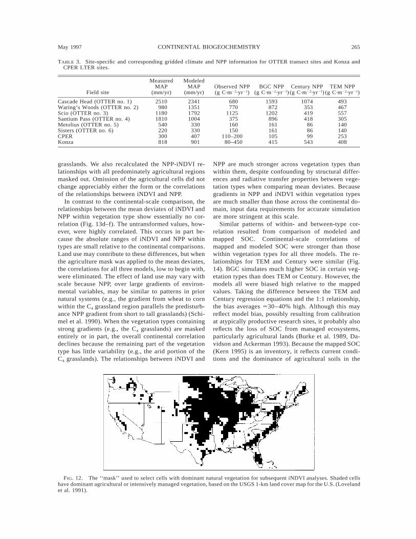
VEMAP simulations were done using a ‘‘potentialnatural’’ vegetation map whereas iNDVI is based on atime series in the 1980s (see Methods) and so reflectsactual land use. To account for this difference we useda recent land cover data base to ‘‘mask out’’ (Fig. 12)

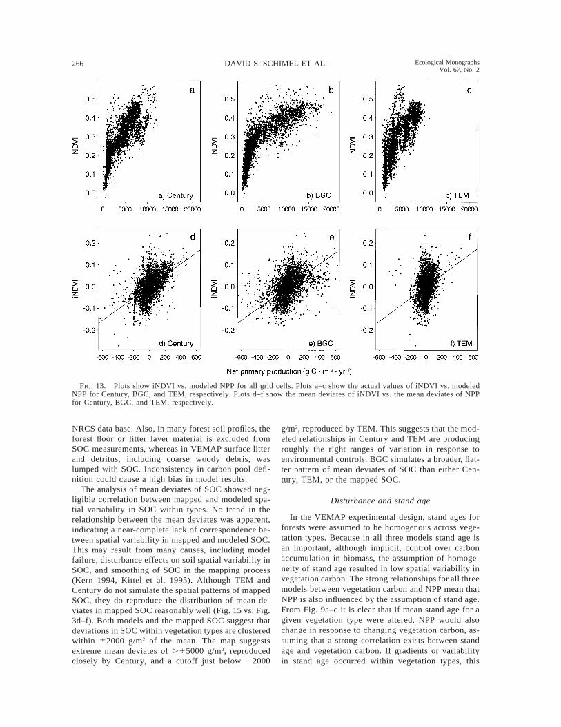
intensively managed land cover types. We then ex-amined iNDVI–NPP relationships for all grid cells(Fig. 13) and only for grid cells dominated by naturalvegetation (data not shown). We examined both actualiNDVI and NPP and the mean deviates of NPP vs. themean deviates of iNDVI to compare the model simu-lations of large-scale vs. within vegetation type vari-ability (Fig. 13). The same analyses were also per-formed for mapped vs. modeled SOC and their meandeviates (Figs. 14 and 15).

The results for the continental-scale comparison ofNPP vs. iNDVI show the two parameters are correlated,even without masking intensive land use regions (Fig.13a–c), with R2s between 0.6 and 0.7 (P , 0.05). Al-though the linear correlations are quite high, the re-lationship between NDVI and NPP is not linear and issteeper at low NPP, and less steep at high NPP (mostevident in BGC and least evident in TEM). The lowerNPP points are predominately grasslands and tundra.The higher points are generally forests. This indicatesthat forest and shrubland/savanna ecosystems can havelarger changes in NPP per unit change in iNDVI than


TABLE 3. Site-specific and corresponding gridded climate and NPP information for OTTER transect sites and Konza andCPER LTER sites.

Field site

MeasuredMAP

(mm/yr)

ModeledMAP

(mm/yr)Observed NPP(g C·m22·yr21)

BGC NPP(g C·m22·yr21)

Century NPP(g C·m22·yr21)

TEM NPP(g C·m22·yr21)

Cascade Head (OTTER no. 1) 2510 2341 680 1593 1074 493Waring’s Woods (OTTER no. 2) 980 1351 770 872 353 467Scio (OTTER no. 3) 1180 1792 1125 1202 419 557Santium Pass (OTTER no. 4) 1810 1004 375 896 418 305Metolius (OTTER no. 5) 540 330 160 161 86 140Sisters (OTTER no. 6) 220 330 150 161 86 140CPER 300 407 110–200 105 99 253Konza 818 901 80–450 415 543 408

FIG. 12. The ‘‘mask’’ used to select cells with dominant natural vegetation for subsequent iNDVI analyses. Shaded cellshave dominant agricultural or intensively managed vegetation, based on the USGS 1-km land cover map for the U.S. (Lovelandet al. 1991).

grasslands. We also recalculated the NPP-iNDVI re-lationships with all predominately agricultural regionsmasked out. Omission of the agricultural cells did notchange appreciably either the form or the correlationsof the relationships between iNDVI and NPP.

In contrast to the continental-scale comparison, therelationships between the mean deviates of iNDVI andNPP within vegetation type show essentially no cor-relation (Fig. 13d–f). The untransformed values, how-ever, were highly correlated. This occurs in part be-cause the absolute ranges of iNDVI and NPP withintypes are small relative to the continental comparisons.Land use may contribute to these differences, but whenthe agriculture mask was applied to the mean deviates,the correlations for all three models, low to begin with,were eliminated. The effect of land use may vary withscale because NPP, over large gradients of environ-mental variables, may be similar to patterns in priornatural systems (e.g., the gradient from wheat to cornwithin the C4 grassland region parallels the predisturb-ance NPP gradient from short to tall grasslands) (Schi-mel et al. 1990). When the vegetation types containingstrong gradients (e.g., the C4 grasslands) are maskedentirely or in part, the overall continental correlationdeclines because the remaining part of the vegetationtype has little variability (e.g., the arid portion of theC4 grasslands). The relationships between iNDVI and

NPP are much stronger across vegetation types thanwithin them, despite confounding by structural differ-ences and radiative transfer properties between vege-tation types when comparing mean deviates. Becausegradients in NPP and iNDVI within vegetation typesare much smaller than those across the continental do-main, input data requirements for accurate simulationare more stringent at this scale.

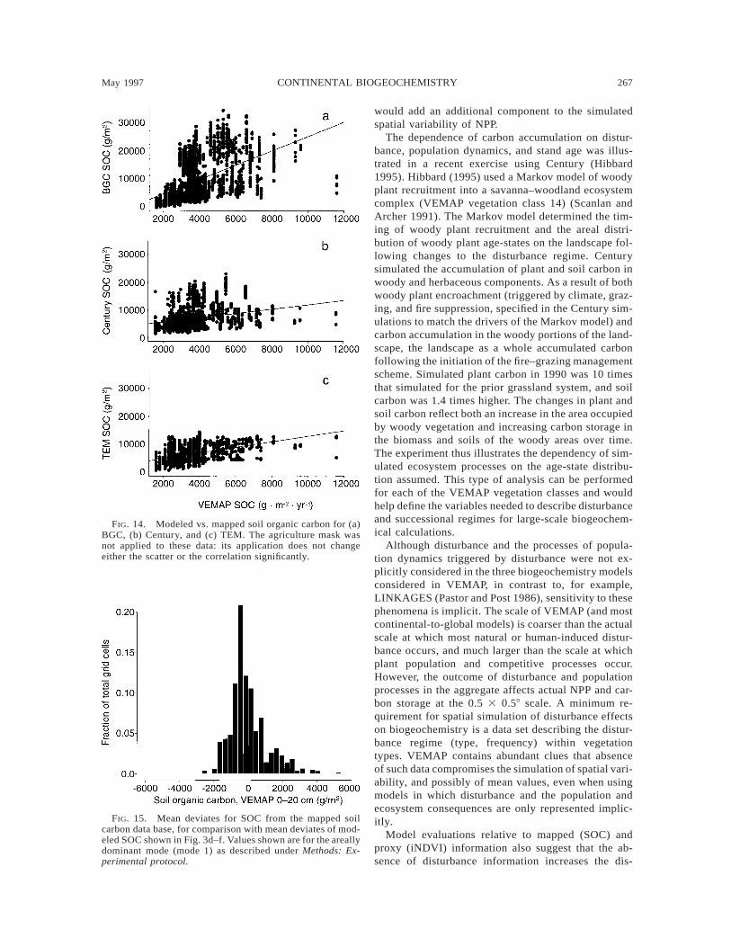
Similar patterns of within- and between-type cor-relation resulted from comparison of modeled andmapped SOC. Continental-scale correlations ofmapped and modeled SOC were stronger than thosewithin vegetation types for all three models. The re-lationships for TEM and Century were similar (Fig.14). BGC simulates much higher SOC in certain veg-etation types than does TEM or Century. However, themodels all were biased high relative to the mappedvalues. Taking the difference between the TEM andCentury regression equations and the 1:1 relationship,the bias averages ø30–40% high. Although this mayreflect model bias, possibly resulting from calibrationat atypically productive research sites, it probably alsoreflects the loss of SOC from managed ecosystems,particularly agricultural lands (Burke et al. 1989, Da-vidson and Ackerman 1993). Because the mapped SOC(Kern 1995) is an inventory, it reflects current condi-tions and the dominance of agricultural soils in the


FIG. 13. Plots show iNDVI vs. modeled NPP for all grid cells. Plots a–c show the actual values of iNDVI vs. modeledNPP for Century, BGC, and TEM, respectively. Plots d–f show the mean deviates of iNDVI vs. the mean deviates of NPPfor Century, BGC, and TEM, respectively.

NRCS data base. Also, in many forest soil profiles, theforest floor or litter layer material is excluded fromSOC measurements, whereas in VEMAP surface litterand detritus, including coarse woody debris, waslumped with SOC. Inconsistency in carbon pool defi-nition could cause a high bias in model results.

The analysis of mean deviates of SOC showed neg-ligible correlation between mapped and modeled spa-tial variability in SOC within types. No trend in therelationship between the mean deviates was apparent,indicating a near-complete lack of correspondence be-tween spatial variability in mapped and modeled SOC.This may result from many causes, including modelfailure, disturbance effects on soil spatial variability inSOC, and smoothing of SOC in the mapping process(Kern 1994, Kittel et al. 1995). Although TEM andCentury do not simulate the spatial patterns of mappedSOC, they do reproduce the distribution of mean de-viates in mapped SOC reasonably well (Fig. 15 vs. Fig.3d–f). Both models and the mapped SOC suggest thatdeviations in SOC within vegetation types are clusteredwithin 62000 g/m2 of the mean. The map suggestsextreme mean deviates of .15000 g/m2, reproducedclosely by Century, and a cutoff just below 22000

g/m2, reproduced by TEM. This suggests that the mod-eled relationships in Century and TEM are producingroughly the right ranges of variation in response toenvironmental controls. BGC simulates a broader, flat-ter pattern of mean deviates of SOC than either Cen-tury, TEM, or the mapped SOC.

Disturbance and stand age

In the VEMAP experimental design, stand ages forforests were assumed to be homogenous across vege-tation types. Because in all three models stand age isan important, although implicit, control over carbonaccumulation in biomass, the assumption of homoge-neity of stand age resulted in low spatial variability invegetation carbon. The strong relationships for all threemodels between vegetation carbon and NPP mean thatNPP is also influenced by the assumption of stand age.From Fig. 9a–c it is clear that if mean stand age for agiven vegetation type were altered, NPP would alsochange in response to changing vegetation carbon, as-suming that a strong correlation exists between standage and vegetation carbon. If gradients or variabilityin stand age occurred within vegetation types, this


FIG. 14. Modeled vs. mapped soil organic carbon for (a)BGC, (b) Century, and (c) TEM. The agriculture mask wasnot applied to these data: its application does not changeeither the scatter or the correlation significantly.

FIG. 15. Mean deviates for SOC from the mapped soilcarbon data base, for comparison with mean deviates of mod-eled SOC shown in Fig. 3d–f. Values shown are for the areallydominant mode (mode 1) as described under Methods: Ex-perimental protocol.

would add an additional component to the simulatedspatial variability of NPP.

The dependence of carbon accumulation on distur-bance, population dynamics, and stand age was illus-trated in a recent exercise using Century (Hibbard1995). Hibbard (1995) used a Markov model of woodyplant recruitment into a savanna–woodland ecosystemcomplex (VEMAP vegetation class 14) (Scanlan andArcher 1991). The Markov model determined the tim-ing of woody plant recruitment and the areal distri-bution of woody plant age-states on the landscape fol-lowing changes to the disturbance regime. Centurysimulated the accumulation of plant and soil carbon inwoody and herbaceous components. As a result of bothwoody plant encroachment (triggered by climate, graz-ing, and fire suppression, specified in the Century sim-ulations to match the drivers of the Markov model) andcarbon accumulation in the woody portions of the land-scape, the landscape as a whole accumulated carbonfollowing the initiation of the fire–grazing managementscheme. Simulated plant carbon in 1990 was 10 timesthat simulated for the prior grassland system, and soilcarbon was 1.4 times higher. The changes in plant andsoil carbon reflect both an increase in the area occupiedby woody vegetation and increasing carbon storage inthe biomass and soils of the woody areas over time.The experiment thus illustrates the dependency of sim-ulated ecosystem processes on the age-state distribu-tion assumed. This type of analysis can be performedfor each of the VEMAP vegetation classes and wouldhelp define the variables needed to describe disturbanceand successional regimes for large-scale biogeochem-ical calculations.

Although disturbance and the processes of popula-tion dynamics triggered by disturbance were not ex-plicitly considered in the three biogeochemistry modelsconsidered in VEMAP, in contrast to, for example,LINKAGES (Pastor and Post 1986), sensitivity to thesephenomena is implicit. The scale of VEMAP (and mostcontinental-to-global models) is coarser than the actualscale at which most natural or human-induced distur-bance occurs, and much larger than the scale at whichplant population and competitive processes occur.However, the outcome of disturbance and populationprocesses in the aggregate affects actual NPP and car-bon storage at the 0.5 3 0.58 scale. A minimum re-quirement for spatial simulation of disturbance effectson biogeochemistry is a data set describing the distur-bance regime (type, frequency) within vegetationtypes. VEMAP contains abundant clues that absenceof such data compromises the simulation of spatial vari-ability, and possibly of mean values, even when usingmodels in which disturbance and the population andecosystem consequences are only represented implic-itly.

Model evaluations relative to mapped (SOC) andproxy (iNDVI) information also suggest that the ab-sence of disturbance information increases the dis-


TABLE 4. Continental-scale totals for NPP and total carbonstorage (vegetation plus soils) for VEMAP models undercurrent climate and CO2 conditions, with the potential nat-ural vegetation shown in Fig. 1.

ModelAnnual NPP(1012 g C/yr)

Totalcarbon storage

(1015 g C)

Biome-BGC 3772 118Century 3125 116TEM 3225 108

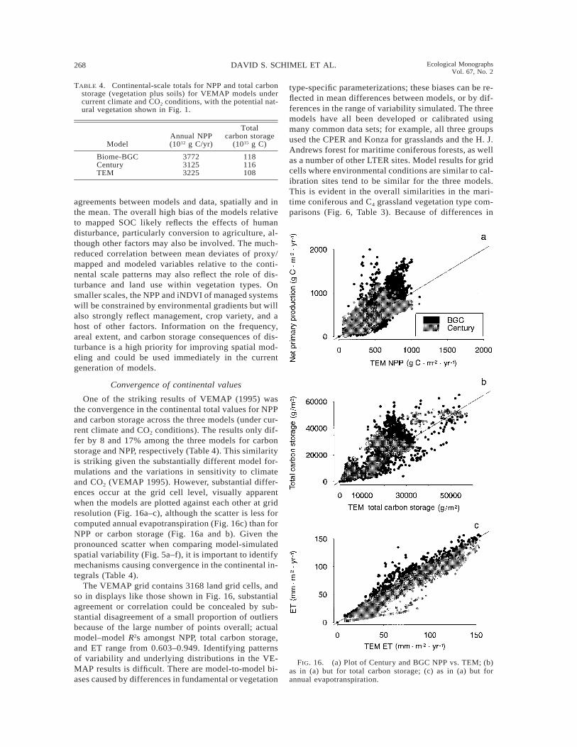
FIG. 16. (a) Plot of Century and BGC NPP vs. TEM; (b)as in (a) but for total carbon storage; (c) as in (a) but forannual evapotranspiration.

agreements between models and data, spatially and inthe mean. The overall high bias of the models relativeto mapped SOC likely reflects the effects of humandisturbance, particularly conversion to agriculture, al-though other factors may also be involved. The much-reduced correlation between mean deviates of proxy/mapped and modeled variables relative to the conti-nental scale patterns may also reflect the role of dis-turbance and land use within vegetation types. Onsmaller scales, the NPP and iNDVI of managed systemswill be constrained by environmental gradients but willalso strongly reflect management, crop variety, and ahost of other factors. Information on the frequency,areal extent, and carbon storage consequences of dis-turbance is a high priority for improving spatial mod-eling and could be used immediately in the currentgeneration of models.

Convergence of continental values

One of the striking results of VEMAP (1995) wasthe convergence in the continental total values for NPPand carbon storage across the three models (under cur-rent climate and CO2 conditions). The results only dif-fer by 8 and 17% among the three models for carbonstorage and NPP, respectively (Table 4). This similarityis striking given the substantially different model for-mulations and the variations in sensitivity to climateand CO2 (VEMAP 1995). However, substantial differ-ences occur at the grid cell level, visually apparentwhen the models are plotted against each other at gridresolution (Fig. 16a–c), although the scatter is less forcomputed annual evapotranspiration (Fig. 16c) than forNPP or carbon storage (Fig. 16a and b). Given thepronounced scatter when comparing model-simulatedspatial variability (Fig. 5a–f), it is important to identifymechanisms causing convergence in the continental in-tegrals (Table 4).

The VEMAP grid contains 3168 land grid cells, andso in displays like those shown in Fig. 16, substantialagreement or correlation could be concealed by sub-stantial disagreement of a small proportion of outliersbecause of the large number of points overall; actualmodel–model R2s amongst NPP, total carbon storage,and ET range from 0.603–0.949. Identifying patternsof variability and underlying distributions in the VE-MAP results is difficult. There are model-to-model bi-ases caused by differences in fundamental or vegetation

type-specific parameterizations; these biases can be re-flected in mean differences between models, or by dif-ferences in the range of variability simulated. The threemodels have all been developed or calibrated usingmany common data sets; for example, all three groupsused the CPER and Konza for grasslands and the H. J.Andrews forest for maritime coniferous forests, as wellas a number of other LTER sites. Model results for gridcells where environmental conditions are similar to cal-ibration sites tend to be similar for the three models.This is evident in the overall similarities in the mari-time coniferous and C4 grassland vegetation type com-parisons (Fig. 6, Table 3). Because of differences in


model sensitivities to input parameters, an extreme val-ue of, for example, soil texture, could cause one modelto generate an extreme SOC, but not another model.An example of this is evident in comparing TEM’s toCentury’s and Biome-BGC’s representation of C4

grasslands, where, because of the choice of calibrationdata (Table 3), TEM’s sensitivity to increasing precip-itation is less than Century’s or Biome-BGC’s. Thiscould allow agreement in the near-modal grid cells, butdisagreement where values vary greatly from the veg-etation class mean, resulting in different spatial pat-terns in the tails of the distributions of NPP or othervariables.

CONCLUSIONS

The models employed in VEMAP simulated spatialvariability in ecosystem processes in substantially dif-ferent ways, with many of the differences resultingfrom each model’s distinct implementation of physicalvs. biogeochemical limitation of NPP. There were alsodifferences in the simulation of soil carbon storage.The evaluation of each model’s simulation of within-type spatial variability shed considerable light on theirdistinctive responses to environmental change, illu-minating the role of climatic vs. biogeochemical con-trols. This substitution of space-for-time (Pickett 1988)within spatial model simulations is a useful check onsteady-state model behavior (Schimel et al. 1990,1994). In all three models, water and nutrient controlsof NPP become correlated at steady state, which inCentury occurs because the water budget strongly in-fluences both the carbon and nitrogen cycles, whereasproduction is jointly limited by water and nitrogenavailability. This is an important insight into modelbehavior, and is consistent with a significant body ofobservations (Zak et al. 1994, Schimel et al. 1996).

The convergence of continental totals likely resultsfrom calibration against overlapping sets of field sites,and the resulting simulation of similar values in siteswith environmental conditions approximating the cal-ibration sites. Differences in sensitivity and spatialvariability within vegetation types, however, are re-flected in the three models’ substantially different sim-ulations of climate change and doubled CO2 effects(VEMAP 1995). Modeled spatial variability and cli-mate sensitivity within vegetation types provided moreinsight into the models’ responses to perturbation thandid examination of spatially aggregated responses (VE-MAP 1995).

Although traditional model evaluation against site-specific measurements is crucial, successful site-spe-cific validation does not guarantee faithful simulationof spatial variability. The use of comprehensive spatialdata sets is a crucial component of assessing simulatedspatial variability, even when the use of comprehensiveinformation requires the use of extrapolated or proxydata. Note that agreement at specific sites in the mar-itime coniferous and C4 grassland types was better than

would be predicted from the distributions of mean de-viates for those types. Proxy and mapped inventorydata are crucial. Comparison of model results withmapped SOC and the integral of the vegetation index(iNDVI) showed the models to have substantially high-er correlations across vegetation types compared towithin vegetation types. This difference does not resultin a simple fashion from land use effects on iNDVI,which, when masked, left the continental-scale corre-lations unaltered but actually reduced the within-typecorrelations. Detailed site-specific data of the type pre-sented for the OTTER and LTER study sites is crucialfor advancing beyond detection of model failure tomodel improvement, because these types of intensivedata provide the information needed to better under-stand underlying processes.

All of the VEMAP ecosystem models are sensitive,implicitly or explicitly, to disturbance and to subse-quent population responses in their simulation of NPPand carbon storage. Both the effects of disturbance (hu-man and natural) and spatial data describing distur-bance regimes are critical aspects of spatial modelingof ecosystems. Improved consideration of disturbanceresponses is a key ‘‘next step’’ for spatial ecosystemmodels.

ACKNOWLEDGMENTS

Data analysis reported in this paper was supported by theNASA EOS program, through an Interdisciplinary Award toDavid S. Schimel. Access to Pathfinder AVHRR was likewiseprovided through NASA. VEMAP is supported by EPRI,NASA’s Mission to Planet Earth Program, and by the U.S.Forest Service. Additional support for VEMAP came fromthe Climate System Modeling Program of UCAR, supportedby the National Science Foundation. The authors also grate-fully acknowledge Elizabeth Sulzman’s assistance with sitedata synthesis. The National Center for Atmospheric Re-search is sponsored by the National Science Foundation. Cli-mate, soil, and vegetation data and climate change scenariosare available through the WorldWide Web: http.//www.cgd.ucar.edu:80/vemap/. The Pathfinder land data set isavailable from http://daac.gsfc.nasa.gov/CAM-PAIGNpDOCS/FTPpSITE/readmes/pal.html/.

LITERATURE CITED

Asrar, G., M. Fuchs, E. T. Kanemasu, and J. L. Hatfield. 1984.Estimating absorbed photosynthetic radiation and leaf areaindex from spectral reflectance in wheat. Agronomy Journal76:300–306.

Bloom, A. J., F. S. Chapin III, and H. A. Mooney. 1985.Resource limitation in plants—an economic analogy. An-nual Review of Ecology and Systematics 16:363–393.

Burke, I. C., T. G. F. Kittel, W. K. Lauenroth, P. Snook, C.M. Yonker, and W. J. Parton. 1991. Regional analysis ofthe central Great Plains. BioScience 41:685–692.

Burke, I. C., and W. K. Lauenroth. 1993. What do LTERresults mean? Extrapolating from site to region and decadeto century. Ecological Modelling 67:19–35.

Burke, I. C., C. M. Yonker, W. J. Parton, C. V. Cole, K. Flach,and D. S. Schimel. 1989. Texture, climate, and cultivationeffects on soil organic matter content in U.S. grasslandsoils. Soil Science Society of America Journal 53:800–805.

Chapin, F. S., III, A. J. Bloom, C. B. Field, and R. H. Waring.1987. Plant responses to multiple environmental factors.BioScience 37:49–57.


Christie, E. K., and J. K. Detling. 1982. Analysis of inter-ference between C3 and C4 grasses in relation to temperatureand soil nitrogen supply. Ecology 63:1277–1284.

Daly, C., R. P. Neilson, and D. L. Phillips. 1994. A statis-tical–topographical model for mapping climatological pre-cipitation over mountainous terrain. Journal of Applied Me-teorology 33:140–158.

Davidson, E. A., and I. L. Ackerman. 1993. Changes in soilcarbon inventories following cultivation of previously un-tilled soils. Biogeochemistry 20:161–193.

Eddy, A. 1987. Interpolated daily surface data: 1881–1985.Oklahoma Climatological Survey. NCAR dataset DS508.0.

Ehleringer, J. R., and C. B. Field, editors. 1993. Scalingphysiological processes leaf to globe. Academic Press, SanDiego, California, USA.

Eisele, K. A., D. S. Schimel, L. A. Kapustka, and W. J. Parton.1989. Effects of available P and N:P ratios on non-sym-biotic dinitrogen fixation in tallgrass prairie soils. Oecol-ogia (Berlin) 79:471–474.

Esser, G. 1986. The carbon budget of the biosphere—struc-ture and preliminary results of the Osnabruck BiosphereModel. Ver offentlichungender Naturforschenden Gesells-chaft in Emden von 1814 7:1–160.

Farqhuar, G. D., S. Von Caemmerer, and J. A. Berry. 1980.A biochemical model of photosynthetic CO2 assimilationin leaves of C3 species. Planta 149:78–90.

Field, C. B. 1991. Ecological scaling of carbon gain to stressand resource availability. Pages 35–65 in H. A. Mooney,W. E. Winner, and E. J. Pell, editors. Response of plantsto multiple stresses. Academic Press, San Diego, Califor-nia, USA.

Fung, I. Y., C. J. Tucker, and K. C. Prentice. 1987. Appli-cation of advanced very high resolution radiometer to studyatmosphere–biosphere exchange of CO2. Journal of Geo-physical Research 92:2999–3015.

Goward, S. N., B. Markham, D. G. Dye, W. Dulaney, and J.Yang. 1991. Normalized difference vegetation index mea-surements from the Advanced Very High Resolution Ra-diometer. Remote Sensing of Environment 35:257–277.

Goward, S. N., C. J. Tucker, and D. G. Dye. 1985. NorthAmerican vegetation patterns observed with the NOAA-7advanced very high resolution radiometer. Vegetatio 64:3–14.

Hibbard, K. 1995. Landscape patterns of carbon and nitrogendynamics in a subtropical savanna: observations and mod-els. Dissertation. Department of Rangeland Ecology andMangement, Texas A&M University, College Station, Tex-as, USA.

Holdridge, L. R. 1967. Life zone ecology. Tropical ScienceCenter, San Jose, Costa Rica.

Holland, E. A., W. J. Parton, J. K. Detling, and D. L. Coppock.1992. Physiological responses of plant populations to her-bivory and their consequences for ecosystem nutrient flow.American Naturalist 140:685–706.

Ingestad, T., and A. B. Lund. 1986. Theory and techniquefor steady state mineral nutrition and growth of plants.Scandinavian Journal of Forest Research 1:439–453.

Kern, J. S. 1994. Spatial patterns of soil organic carbon inthe contiguous United States. Soil Science Society ofAmerica Journal 58:439–455.

. 1995. Geographic patterns of soil water-holding ca-pacity in the contiguous United States. Soil Science Societyof America Journal 59:1126–1133.

Kittel, T. G. F., N. A. Rosenbloom, T. H. Painter, D. S. Schi-mel, and VEMAP Modeling Participants. 1995. The VE-MAP integrated database for modeling United States eco-system/vegetation sensitivity to climate change. Journal ofBiogeography 22:857–862.

Kuchler, A. W. 1964. Manual to accompany the map, po-tential natural vegetation of the coterminous United States.

Second edition. Special Publication Number 36. AmericanGeographical Society, New York, New York, USA.

Law, B. E., and R. H. Waring. 1994. Combining remotesensing and climatic data to estimate net primary produc-tion across Oregon. Ecological Applications 4:717–728.

Lieth, H. 1972. Modelling the primary productivity of theworld. Nature and Resources 8:5–10.

Loveland, T. R., J. W. Merchant, D. O. Ohlen, and J. F. Brown.1991. Development of a land-cover characteristics data-base for the conterminous U.S. Photogrammetric Engi-neering and Remote Sensing 57:1453–1463.

McGuire, A. D., L. A. Joyce, D. W. Kicklighter, J. M. Melillo,G. Esser, and C. J. Vorosmarty. 1993. Productivity re-sponse of climax temperate forests to elevated temperatureand carbon dioxide: A North American comparison be-tween two global models. Climatic Change 24:287–310.

Melillo, J. M., R. J. Naiman, J. D. Aber, and A. E. Linkins.1984. Factors controlling mass loss and nitrogen dynamicsof plant litter decaying in northern streams. Bulletin ofMarine Science 35:341–356.

Milchunas, D. G., and W. K. Lauenroth. 1992. Carbon dy-namics and estimates of primary production by harvest, 14Cdilution, and 14C turnover. Ecology 73:593–607.

NCDC. 1992. 1961–1990 monthly station normals tape. Na-tional Climatic Data Center, U.S. Department of Com-merce, data tape TD 9641.

Nobel, P. S. 1991. Physicochemical and environmental plantphysiology. Academic Press, San Diego, California, USA.

Parton, W. J., D. S. Ojima, C. V. Cole, and D. S. Schimel.1994. A general model for soil organic matter dynamics:sensitivity to litter chemistry, texture and management.Pages 147–167 in Quantitative modeling of soil formingprocesses. Soil Science Society of America, Madison, Wis-consin, USA.

Parton, W. J., D. S. Schimel, C. V. Cole, and D. S. Ojima.1987. Analysis of factors controlling soil organic matterlevels in Great Plains grasslands. Soil Science Society ofAmerica Journal 51:1173–1179.

Pastor, J., and W. M. Post. 1986. Influence of climate, soilmoisture and succession on forest carbon and nitrogen cy-cles. Biogeochemistry 2:3–27.

Pickett, S. T. A. 1988. Space-for-time substitution as an al-ternative to long-term studies. Pages 110–135 in G. E. Lik-ens, editor. Long-term studies in ecology: approaches andalternatives. Springer-Verlag, New York, New York, USA.

Potter, C. S., J. T. Randerson, C. B. Field, P. A. Matson, P.M. Vitousek, H. A. Mooney, and S. A. Klooster. 1993.Terrestrial ecosystem production: a process model basedon global satellite and surface data. Global BiogeochemicalCycles 7:811–841.

Richardson, C. W., and D. A. Wright. 1984. WGEN: a modelfor generating daily weather variables. U.S. Department ofAgriculture, Agricultural Research Service, ARS-8.

Running, S. W. 1994. Testing forest-BGC ecosystem processsimulations across a climatic gradient in Oregon. Ecolog-ical Applications 4:238–247.

Running, S. W., and E. R. Hunt, Jr. 1993. Generalization ofa forest ecosystem model for other biomes, BIOME-BGC,and an application for global-scale models. Pages 141–158in J. R. Ehleringer and C. B. Field, editors. Scaling phys-iological processes: leaf to globe. Academic Press, SanDiego, California, USA.

Running, S. W., and R. R. Nemani. 1991. Regional hydrolicand carbon balance responses of forests resulting from po-tential climate change. Climatic Change 19:349–368.

Runyon, J., R. H. Waring, S. N. Goward, and J. M. Welles.1994. Environmental limits on net primary production andlight-use efficiency across the Oregon Transect. EcologicalApplications 4:226–237.

Sala, O. E., W. J. Parton, L. A. Joyce, and W. K. Lauenroth.


1988. Primary production of the central grasslands regionof the United States: spatial pattern and major controls.Ecology 69:40–45.

Scanlan, J. C., and S. Archer. 1991. Simulated dynamics ofsuccession in a North American subtropical Prosopis sa-vanna. Journal of Vegetation Science 2:625–634.

Schimel, D. S., B. H. Braswell Jr., E. A. Holland, R. Mc-Keown, D. S. Ojima, T. H. Painter, W. J. Parton, and A. R.Townsend. 1994. Climatic, edaphic, and biotic controlsover carbon and turnover of carbon in soils. Global Bio-geochemical Cycles 8:279–293.

Schimel, D. S., B. H. Braswell, R. McKeown, D. S. Ojima,W. J. Parton, and W. Pulliam. 1996. Climate and nitrogencontrols on the geography and time scales of terrestrialbiogeochemical cycling. Global Biogeochemical Cycles10:677–692.

Schimel, D. S., T. G. F. Kittel, and W. J. Parton. 1991. Ter-restrial biogeochemical cycles: Global interactions with at-mosphere and hydrology. Tellus 43AB:188–203.

Schimel, D. S., W. J. Parton, T. G. F. Kittel, D. S. Ojima, andC. V. Cole. 1990. Grassland biogeochemistry: links to at-mospheric processes. Climatic Change 17:13–25.

Schimel, D. S., and C. S. Potter. 1995. Process modellingand spatial extrapolation. Pages 358–383 in P. A. Matsonand R. C. Harriss, editors. Biogenic trace gases: measuringemissions from soil and water. Blackwell Science, Cam-bridge, Massachusetts, USA.

Schimel, D. S., M. A. Stillwell, and R. G. Woodmansee.1985. Biogeochemistry of C, N, and P in a soil catena ofthe shortgrass steppe. Ecology 66:276–282.

Sellers, P. J. 1985. Canopy reflectance, photosynthesis andtranspiration. International Journal of Remote Sensing 6:1335–1372.

Thornley, J. H. M. 1972. A balanced quantitative model forroot:shoot ratios in vegetative plants. Annals of Botany 36:419–430.

Tilman, D. 1985. The resource-ratio hypothesis of plant suc-cession. American Naturalist 125:827–852.

Tucker, C. J. 1979. Red and photographic infrared linearcombinations for monitoring vegetation. Remote Sensingof Environment 8:127–150.

Tucker, C. J., I. Y. Fung, C. D. Keeling, and R. H. Gammon.1986. Relationship between atmospheric CO2 variationsand a satellite-derived vegetation index. Nature 319:195–199.

VEMAP Participants. 1995. Vegetation/Ecosystem modelingand analysis project (VEMAP): comparing biogeographyand biogeochemistry models in a continental-scale studyof terrestrial ecosystem responses to climate change andCO2 doubling. Global Biogeochemical Cycles 9:407–438.

Wedin, D. A., and D. Tilman. 1990. Species effects on ni-trogen cycling: a test with perennial grasses. Oecologia(Berlin) 84:433–441.

Whittaker, R. H. 1975. Communities and ecosystems. Mac-Millan, New York, New York, USA.

Zak, D. R., D. Tilman, R. R. Parmenter, C. W. Rice, F. M.Fisher, J. Vose, D. Milchunas, and C. W. Martin. 1994.Plant production and soil microorganisms in late-succes-sional ecosystems: a continental-scale study. Ecology 75:2333–2347.

CONTINENTAL SCALE VARIABILITY IN ECOSYSTEM · PDF fileCONTINENTAL SCALE VARIABILITY IN...

Documents

Transcript of CONTINENTAL SCALE VARIABILITY IN ECOSYSTEM · PDF fileCONTINENTAL SCALE VARIABILITY IN...