CONTEXT-AWARE WIRELESS NETWORKS - unibo.it
273
ALMA MATER STUDIORUM UNIVERSIT ` A DEGLI STUDI DI BOLOGNA Dottorato di Ricerca in Ingegneria Elettronica, Informatica e delle Telecomunicazioni Dipartimento di Ingegneria dell’Energia Elettrica e dell’Informazione “Guglielmo Marconi” Ciclo XXV Settore concorsuale: 09/F2 - TELECOMUNICAZIONI Settore scientifico disciplinare: ING-INF/03 - TELECOMUNICAZIONI CONTEXT-AWARE WIRELESS NETWORKS Tesi presentata da: NICOL ´ O DECARLI Coordinatore Dottorato: Chiar.mo Prof. Ing. ALESSANDRO VANELLI-CORALLI Relatori: Chiar.mo Prof. Ing. MARCO CHIANI Chiar.mo Prof. Ing. DAVIDE DARDARI ESAME FINALE 2013
Transcript of CONTEXT-AWARE WIRELESS NETWORKS - unibo.it

ALMA MATER STUDIORUMUNIVERSIT A DEGLI STUDI DI BOLOGNA
Dottorato di Ricerca in Ingegneria Elettronica, Informati ca edelle Telecomunicazioni
Dipartimento di Ingegneria dell’Energia Elettrica edell’Informazione “Guglielmo Marconi”
Ciclo XXV
Settore concorsuale:09/F2 - TELECOMUNICAZIONI
Settore scientifico disciplinare:ING-INF/03 - TELECOMUNICAZIONI
CONTEXT-AWARE WIRELESSNETWORKS
Tesi presentata da:NICOLO DECARLI
Coordinatore Dottorato:Chiar.mo Prof. Ing.
ALESSANDROVANELLI-CORALLI
Relatori:
Chiar.mo Prof. Ing.MARCO CHIANI
Chiar.mo Prof. Ing.DAVIDE DARDARI
ESAME FINALE 2013

INDEX TERMS
UWB
Time Delay Estimation
Localization
Relay
RFID

Contents
Introduction 1
I Non-Coherent Signal Demodulation 9
1 Integration Time Optimization in Non-Coherent Receivers 131.1 Motivations . . . . . . . . . . . . . . . . . . . . . . . . . . . . 131.2 Signal and Channel Models . . . . . . . . . . . . . . . . . . . 14
1.2.1 Transmitted-Reference Signaling . . . . . . . . . . . . . 141.2.2 Channel Model . . . . . . . . . . . . . . . . . . . . . . 151.2.3 Autocorrelation Receiver Structure . . . . . . . . . . . 15
1.3 Integration Time Determination . . . . . . . . . . . . . . . . . 161.4 Numerical Results . . . . . . . . . . . . . . . . . . . . . . . . . 211.5 Conclusion . . . . . . . . . . . . . . . . . . . . . . . . . . . . . 23
2 Stop-and-Go Receivers 252.1 Motivations . . . . . . . . . . . . . . . . . . . . . . . . . . . . 252.2 Signal and Channel Model . . . . . . . . . . . . . . . . . . . . 26
2.2.1 TR-BPAM . . . . . . . . . . . . . . . . . . . . . . . . . 262.2.2 BPPM . . . . . . . . . . . . . . . . . . . . . . . . . . . 272.2.3 Channel Model . . . . . . . . . . . . . . . . . . . . . . 28
2.3 Stop-and-Go Receivers . . . . . . . . . . . . . . . . . . . . . . 282.3.1 Conventional AcR . . . . . . . . . . . . . . . . . . . . 282.3.2 Conventional EDR . . . . . . . . . . . . . . . . . . . . 302.3.3 SaG Receivers . . . . . . . . . . . . . . . . . . . . . . . 31
2.4 Performance Evaluation . . . . . . . . . . . . . . . . . . . . . 332.4.1 SaG-AcR . . . . . . . . . . . . . . . . . . . . . . . . . 332.4.2 SaG-EDR . . . . . . . . . . . . . . . . . . . . . . . . . 36
2.5 Bin Selection Strategies for the SaG Receivers . . . . . . . . . 382.5.1 Threshold-Based Bin Selection Strategy . . . . . . . . 402.5.2 Blind Bin Selection Strategy . . . . . . . . . . . . . . . 44
iii

2.6 Numerical Results . . . . . . . . . . . . . . . . . . . . . . . . . 462.7 Conclusion . . . . . . . . . . . . . . . . . . . . . . . . . . . . . 52
II Time-Delay Estimation 53
3 Bounds on Time-Delay Estimation 573.1 Motivations . . . . . . . . . . . . . . . . . . . . . . . . . . . . 573.2 Signal Model . . . . . . . . . . . . . . . . . . . . . . . . . . . 603.3 The Ziv-Zakai Lower Bound . . . . . . . . . . . . . . . . . . . 633.4 ZZB for Known Signals . . . . . . . . . . . . . . . . . . . . . . 64
3.4.1 Average ZZB . . . . . . . . . . . . . . . . . . . . . . . 663.5 ZZB for Signals with Unknown Phase . . . . . . . . . . . . . . 66
3.5.1 Asymptotic ZZB . . . . . . . . . . . . . . . . . . . . . 683.6 ZZB for Unknown Deterministic Signals . . . . . . . . . . . . 68
3.6.1 Detector Design . . . . . . . . . . . . . . . . . . . . . . 693.6.2 Detector Performance . . . . . . . . . . . . . . . . . . . 703.6.3 Asymptotic ZZB . . . . . . . . . . . . . . . . . . . . . 77
3.7 ML TOA Estimators . . . . . . . . . . . . . . . . . . . . . . . 783.7.1 ML TOA Estimation of Known Signals . . . . . . . . . 783.7.2 ML TOA Estimation of Signals with Unknown Phase . 793.7.3 ML TOA Estimation of Unknown Deterministic Signals 79
3.8 Numerical Results . . . . . . . . . . . . . . . . . . . . . . . . . 793.9 Conclusion . . . . . . . . . . . . . . . . . . . . . . . . . . . . . 813.A Series Expansions of Signals . . . . . . . . . . . . . . . . . . . 82
3.A.1 Series Expansion of Baseband Random Signals . . . . . 823.A.2 Series Expansion of Bandpass Random Signals . . . . . 843.A.3 Series Expansion of Baseband Deterministic Signals . . 853.A.4 Series Expansion of Bandpass Deterministic Signals . . 86
3.B Proof of Equation (3.11) . . . . . . . . . . . . . . . . . . . . . 873.C Asymptotic Expression of Pmin (z) . . . . . . . . . . . . . . . . 873.D Derivation of P {Y1 < Y2} . . . . . . . . . . . . . . . . . . . . . 88
III Location-Awareness 91
4 Experimentation for Cooperative Localization 954.1 Motivations . . . . . . . . . . . . . . . . . . . . . . . . . . . . 954.2 Network Experimentation Methodology . . . . . . . . . . . . . 97
4.2.1 Network Geometry . . . . . . . . . . . . . . . . . . . . 984.2.2 Links Characterization . . . . . . . . . . . . . . . . . . 100
iv

4.2.3 Obstacles Characterization . . . . . . . . . . . . . . . . 101
4.3 Range Error Model . . . . . . . . . . . . . . . . . . . . . . . . 102
4.4 Harnessing Environmental Information . . . . . . . . . . . . . 104
4.4.1 Previous Works . . . . . . . . . . . . . . . . . . . . . . 105
4.4.2 Channel State Identification Algorithms . . . . . . . . 106
4.4.3 Experimental Results . . . . . . . . . . . . . . . . . . . 109
4.5 Conclusion . . . . . . . . . . . . . . . . . . . . . . . . . . . . . 111
5 Relaying Techniques for Network Localization 113
5.1 Motivations . . . . . . . . . . . . . . . . . . . . . . . . . . . . 113
5.2 System Model . . . . . . . . . . . . . . . . . . . . . . . . . . . 115
5.2.1 Non-Regenerative Relays . . . . . . . . . . . . . . . . . 115
5.2.2 Signal Model . . . . . . . . . . . . . . . . . . . . . . . 116
5.3 Localization with Non-Regenerative Relays . . . . . . . . . . . 119
5.3.1 ML Localization with Perfect CSI (Estimator A) . . . 119
5.3.2 ML Localization with Partial CSI . . . . . . . . . . . . 121
5.4 Case Study . . . . . . . . . . . . . . . . . . . . . . . . . . . . 127
5.4.1 Scenario . . . . . . . . . . . . . . . . . . . . . . . . . . 127
5.4.2 Performance Metrics . . . . . . . . . . . . . . . . . . . 130
5.4.3 Simulation Results . . . . . . . . . . . . . . . . . . . . 130
5.5 Conclusion . . . . . . . . . . . . . . . . . . . . . . . . . . . . . 133
5.A Derivation of the ML estimator . . . . . . . . . . . . . . . . . 134
5.B Derivation of the ML estimator . . . . . . . . . . . . . . . . . 135
5.C Derivation of the ML estimator . . . . . . . . . . . . . . . . . 136
IV A Case-Study: The UWB-RFID System 141
6 System Overview 145
6.1 Introduction . . . . . . . . . . . . . . . . . . . . . . . . . . . . 145
6.2 UWB Backscattering Principle . . . . . . . . . . . . . . . . . . 146
6.3 System Architecture and Main Functionalities . . . . . . . . . 147
6.3.1 Tags Synchronization . . . . . . . . . . . . . . . . . . . 151
6.3.2 Readers Synchronization . . . . . . . . . . . . . . . . . 152
6.3.3 Tag Detection . . . . . . . . . . . . . . . . . . . . . . . 153
6.3.4 Signal Demodulation . . . . . . . . . . . . . . . . . . . 154
6.3.5 Time of Arrival Estimation . . . . . . . . . . . . . . . 155
6.3.6 Localization . . . . . . . . . . . . . . . . . . . . . . . . 155
6.3.7 Untagged Object Detection and Tracking . . . . . . . . 155
v
7 Performance Analysis in Ideal Conditions 1577.1 Motivations . . . . . . . . . . . . . . . . . . . . . . . . . . . . 1577.2 Backscatter Communication using UWB Signals . . . . . . . . 1577.3 Multiple Users Interference and Clutter . . . . . . . . . . . . . 161
7.3.1 Perfect Timing Acquisition . . . . . . . . . . . . . . . . 1637.4 Code Choice for Clutter Removal and Multiple Access . . . . 1647.5 Numerical Results . . . . . . . . . . . . . . . . . . . . . . . . . 165
7.5.1 BER Analysis with Measured Signals . . . . . . . . . . 1657.5.2 BER Analysis in the 802.15.4a Channel . . . . . . . . . 166
7.6 Conclusion . . . . . . . . . . . . . . . . . . . . . . . . . . . . . 167
8 System Design and in Presence of Hardware Constraints 1698.1 Motivations . . . . . . . . . . . . . . . . . . . . . . . . . . . . 1698.2 Backscatter Communication . . . . . . . . . . . . . . . . . . . 170
8.2.1 Transmitted Signal Format . . . . . . . . . . . . . . . . 1718.2.2 Tag-to-Reader Communication . . . . . . . . . . . . . 1718.2.3 Signal De-Spreading . . . . . . . . . . . . . . . . . . . 172
8.3 Tags Code Assignment Strategies . . . . . . . . . . . . . . . . 1758.4 Tag Detection . . . . . . . . . . . . . . . . . . . . . . . . . . . 179
8.4.1 Tag Detection Scheme . . . . . . . . . . . . . . . . . . 1798.4.2 Threshold Evaluation Criteria . . . . . . . . . . . . . . 181
8.5 Numerical Results . . . . . . . . . . . . . . . . . . . . . . . . . 1878.5.1 Simulation Parameters . . . . . . . . . . . . . . . . . . 1878.5.2 System Design . . . . . . . . . . . . . . . . . . . . . . 1878.5.3 Results in Multi-Tags Scenario . . . . . . . . . . . . . . 190
8.6 Implementation Issues . . . . . . . . . . . . . . . . . . . . . . 1928.6.1 Receiver Dynamic Range . . . . . . . . . . . . . . . . . 1928.6.2 Multi-Reader Interference . . . . . . . . . . . . . . . . 1958.6.3 Analog-to-Digital Conversion . . . . . . . . . . . . . . 197
8.7 Conclusion . . . . . . . . . . . . . . . . . . . . . . . . . . . . . 1998.A Effect of De-Spreading on A/D Conversion . . . . . . . . . . . 199
9 Theoretical Bounds on the Localization Accuracy 2059.1 Motivations . . . . . . . . . . . . . . . . . . . . . . . . . . . . 2059.2 System Model . . . . . . . . . . . . . . . . . . . . . . . . . . . 205
9.2.1 Ranging Models and Localization . . . . . . . . . . . . 2079.2.2 Ranging Error and System Parameters . . . . . . . . . 208
9.3 Localization Performance Bounds . . . . . . . . . . . . . . . . 2099.3.1 Monostatic Networks . . . . . . . . . . . . . . . . . . . 2109.3.2 Multistatic Networks . . . . . . . . . . . . . . . . . . . 212
9.4 Case Studies . . . . . . . . . . . . . . . . . . . . . . . . . . . . 215
vi
9.4.1 System Parameters . . . . . . . . . . . . . . . . . . . . 2159.4.2 PEB in the 2D Scenario . . . . . . . . . . . . . . . . . 2159.4.3 Localization Error Outage . . . . . . . . . . . . . . . . 217
9.5 Conclusions . . . . . . . . . . . . . . . . . . . . . . . . . . . . 220
Conclusions 223
vii

viii

List of Figures
1 Context-aware wireless network. . . . . . . . . . . . . . . . . . 3
1.1 Conventional autocorrelation receiver. . . . . . . . . . . . . . . 161.2 AcR with proposed integration time estimation. . . . . . . . . 171.3 BEP for the TR AcR (exp. PDP). . . . . . . . . . . . . . . . 221.4 BEP for the TR AcR (CM4). . . . . . . . . . . . . . . . . . . 22
2.1 Conventional non-coherent receivers. . . . . . . . . . . . . . . 292.2 Stop-and-go receivers. . . . . . . . . . . . . . . . . . . . . . . 302.3 Decision device (DEC). . . . . . . . . . . . . . . . . . . . . . . 312.4 Conditional BEP of the SaG receiver as a function of the ASNR. 392.5 Required ASNR improvement ∆γ as function of the ASNR γ. 432.6 Performance as function of the number of accumulations Na. . 472.7 Performance as function of the integration time TED. . . . . . 472.8 Performance for different number k for noise PSD estimation. 482.9 Performance with fixed threshold ξ. . . . . . . . . . . . . . . . 492.10 Performance with fixed threshold TNR = 4dB. . . . . . . . . . 502.11 Performance with different bin selection strategies. . . . . . . . 51
3.1 Results for lowpass signals. . . . . . . . . . . . . . . . . . . . . 803.2 Results for lowpass signals. . . . . . . . . . . . . . . . . . . . . 81
4.1 The experimentation environments. . . . . . . . . . . . . . . . 974.2 Connectivity matrix for the environment B. . . . . . . . . . . 984.3 Network experimentation environment. . . . . . . . . . . . . . 994.4 Example of measured waveforms. . . . . . . . . . . . . . . . . 1004.5 Obstacles characterization setup. . . . . . . . . . . . . . . . . 1014.6 Range error bias for nodes pairs in LOS or NLOS conditions. . 1034.7 Relative frequency for delay spread in LOS and NLOS. . . . . 109
5.1 Example of localization system employing relays. . . . . . . . 1155.2 Non-regenerative relays. . . . . . . . . . . . . . . . . . . . . . 1165.3 Example of signal structure in a scenario adopting active tags. 119
ix
5.4 Scenario considered in the simulation results. . . . . . . . . . . 1285.5 LEO for a softer multipath channel. . . . . . . . . . . . . . . . 1315.6 LEO for a stronger multipath channel. . . . . . . . . . . . . . 1325.7 RMSE contour map in the 2D environment. . . . . . . . . . . 1335.8 c.d.f.s of the RMSE. . . . . . . . . . . . . . . . . . . . . . . . 134
6.1 Application scenario. . . . . . . . . . . . . . . . . . . . . . . . 1466.2 Example of a square cell monitored by four readers. . . . . . . 1476.3 Example of backscattered signal. . . . . . . . . . . . . . . . . 1486.4 Signal contributions at the reader port. . . . . . . . . . . . . . 1496.5 SELECT general system architecture. . . . . . . . . . . . . . . 1506.6 UWB reader architecture in backscattering schemes. . . . . . . 1516.7 UWB tag architecture in backscattering schemes. . . . . . . . 1526.8 Backscatter modulation. . . . . . . . . . . . . . . . . . . . . . 1536.9 Wake-up scheme. . . . . . . . . . . . . . . . . . . . . . . . . . 1546.10 UHF-UWB interrogation cycle. . . . . . . . . . . . . . . . . . 154
7.1 The considered scheme of tag reader. . . . . . . . . . . . . . . 1587.2 Backscatter signal structure. . . . . . . . . . . . . . . . . . . . 1617.3 Indoor scenario considered for the measurement campaign. . . 1657.4 BER in multi-tag laboratory environment. . . . . . . . . . . . 1667.5 BER in multipath 802.15.4a CM1 channel. . . . . . . . . . . . 167
8.1 Reader internal structure. . . . . . . . . . . . . . . . . . . . . 1708.2 Example of energy matrix. . . . . . . . . . . . . . . . . . . . . 1818.3 Minimum number of pulses per symbol. . . . . . . . . . . . . . 1898.4 ROC for the tag detection in UWB backscatter system. . . . . 1918.5 ROC for tag detection in presence of synchronization offset. . 1928.6 Typical dynamic range of a UWB-RFID system. . . . . . . . . 1948.7 SQNR at the ADC output. . . . . . . . . . . . . . . . . . . . . 1988.8 The considered scheme for the ADC and de-spreader. . . . . . 2008.9 SQNR gain after de-spreading and accumulation. . . . . . . . 202
9.1 Network configurations. . . . . . . . . . . . . . . . . . . . . . 2069.2 PEB, configuration #1. . . . . . . . . . . . . . . . . . . . . . 2169.3 PEB, configuration #2. . . . . . . . . . . . . . . . . . . . . . 2169.4 PEB, configuration #3. . . . . . . . . . . . . . . . . . . . . . 2179.5 PEB, configuration #4. . . . . . . . . . . . . . . . . . . . . . 2189.6 PEB, configuration #5. . . . . . . . . . . . . . . . . . . . . . 2199.7 Localization error outage (1). . . . . . . . . . . . . . . . . . . 2209.8 Localization error outage (2). . . . . . . . . . . . . . . . . . . 221
x

List of Tables
4.1 Mean and standard deviation of ranging bias. . . . . . . . . . 1024.2 Mean bias, standard deviation and frequency. . . . . . . . . . 1044.3 Classical identification approach. . . . . . . . . . . . . . . . . 1104.4 Distribution-based identification approach. . . . . . . . . . . . 110
8.1 Clutter rejection and process gain properties of odd codes. . . 1768.2 Interference mitigation properties of PN codes. . . . . . . . . . 177
xi

xii

List of Acronyms
AcF autocorrelation function
AcR autocorrelation receiver
ADC analog-to-digital converter
AF amplify & forward
AI automatic identification
AIC Akaike information criterion
AOA angle-of-arrival
AOT approximate optimum threshold
ASNR accumulated signal-to-noise ratio
AWGN additive white Gaussian noise
BEP bit error probability
BER bit error rate
BIC Bayesian information criterion
BPAM binary pulse amplitude modulation
BPPM binary pulse position modulation
BPZF band-pass zonal filter
c.d.f. cumulative distribution function
CAIC consistent Akaike information criterion
CcF crosscorrelation function
xiii
CDMA code division multiple access
CEOT channel ensemble optimum threshold
CIR channel impulse response
CR channel response
CRB Cramer-Rao bound
CSI channel state information
CW continuous wave
DBPSK differential binary phase shift keying
DF detect & forward
DP direct path
DS-SS direct-sequence spread-spectrum
ED energy detector
EDR energy detector receiver
EIRP effective radiated isotropic power
ELP equivalent low-pass
FCC Federal Communications Commission
FIM Fisher information matrix
GLRT generalized likelihood ratio test
GPS global positioning system
HPBW half power beam width
INR interference-to-noise ratio
IR impulse radio
ISI inter-symbol interference
isi intra-symbol interference
ISNR interference-plus-signal-to-noise-ratio
xiv

ITC information theoretic criteria
JF just forward
KL Karhunen-Loeve
LEO localization error outage
LNA low-noise amplifier
LOS line-of-sight
LRT likelihood ratio test
LS least squares
MAC medium access control
MF matched filter
ML maximum likelihood
MPC multipath component
MSE mean squared error
MUI multi-user interference
NLOS non-line-of-sight
OOK on-off keying
OT optimum threshold
p.d.f. probability density function
PAM pulse amplitude modulation
PD probability of detection
PDP power delay profile
PEB position error bound
PFA probability of false alarm
PN pseudo-noise
PPM pulse position modulation
xv

PRP pulse repetition period
PSD power spectral density
r.v. random variable
RCS radar cross section
RFID radio-frequency identification
rms root mean square
RMSE root-mean-square error
ROC receiver operating characteristic
RRC root raised cosine
RSN radar sensor network
RSSI received signal strength indicator
RTLS real time locating systems
SaG stop-and-go
SCM supply chain management
SNR signal-to-noise ratio
SPMF single-path matched filter
SQNR signal-to-quantization-noise ratio
TDE time delay estimation
TDMA time division multiple access
TDOA time difference-of-arrival
TH time-hopping
TNR threshold-to-noise ratio
TOA time-of-arrival
TR transmitted-reference
UHF ultra-high frequency
xvi

UWB ultrawide-band
VGA variable-gain amplifier
WED wall extra delay
WSN wireless sensor network
WSR wireless sensor radar
WSS wide-sense stationary
WWB Weiss-Weinstein bound
ZZB Ziv-Zakai bound
xvii

xviii
Introduction
Motivations
In the last decades the introduction of pervasive wireless technology revolu-tionized our daily life making available in almost any time and in any placeservices able to guarantee communication between people. More recentlywireless devices introduced the possibility of connecting to the Internet net-work not only indoor when using fixed workstations, but also in mobile en-vironments, enabling a myriad of new services capable of sharing data andproviding real time information to the end user. Contextually mobile de-vices, for example cellphones, increased their computational capabilities anddifferent technologies, such as global positioning system (GPS) were incor-porated in the same apparatus, opening for the first time the possibility oflocation-based services, now more and more interconnected with the Inter-net world. The innovation in wireless computing did not involve the mobiledevices for end users only, but also the professional market, as in the caseof mobile computing for logistic applications. In this field we faced on theintroduction of the concept of “Internet of Things”, defined by MIT Auto-IDLabs, according to which the physical world will be mapped into the Internetspace, thus enabling a potentially huge number of novel applications [1, 2, 3].Ideally, it is expected that every object in our every-day life will be assignedto an IP address and will be responsive to the presence of people. Fromthe technological point of view, a key enabling technology is represented byradio-frequency identification (RFID) [4].
The next technological step could be represented by the increasing of ag-gregation of different technologies and paradigms, enabling services strictlyrelated to the environment in which the device is operating, whatever itsnature is. This is the concept of context-aware networks. Context-awarenesshas been introduced in several fields related to wireless services, involvingevery stack layer, from the physical one to applications. The ideas behindcontext-aware computing have been presented in [5] where the author in-dicates a phenomenon for which computing takes into account the natural
1

human environment and allows the computers themselves to vanish into thebackground. The term was firstly adopted in [6] referring to systems thatadapt according to their location of use, the collection of nearby people andobjects, as well as changes to those objects over time [7].
The context information can serve on one hand to drive, as anticipated,future applications and services, and on the other hand to improve the net-work efficiency itself. Examples of both applications can be find in the ideasof context-aware approaches to wireless transmission adaptation [8], context-aware wireless sensor networks [9], context-aware and adaptive security [10]and in a myriad of context-aware applications for monitoring, sensing, secu-rity, emergencies, multimedia services [11, 12, 13, 14, 15, 16, 17, 18, 19, 20].
From these works it emerges how the context-awareness, also when in-tended at application level, implies ad-hoc functionalities that the technologymust provide [21, 8, 9, 22, 23]. In fact, context-aware applications need differ-ent kinds of information sources. In particular the two pillars are representedby the location information (from which the concept of location-awareness isoften derived) and the sensors embedded in the devices able to provide dataregarding the surrounding environment. Although available services suchas GPS can provide accurate location information in outdoor environment,context-aware networking often requires the availability of this informationanywhere and anytime, indoor environments included. Indoor positioningis much more challenging than outdoor and, in recent years, an importantresearch activity has been carried out in order to design practical schemescapable of dealing with the main limitations deriving from the propagationenvironment and the fact that positioning must be guaranteed in many casesby already existing technologies not originally developed for this kind of ser-vice. Localization is usually realized by an infrastructure including taggednodes (agents or tags) attached to or embedded in objects and of referencenodes (anchors) placed in known positions, which communicate with tagsthrough wireless signals to determine their locations [24].
Figure 1 shows an example of context-aware network where several en-tities are involved. Specifically, we have a set of mobile or fixed referencenodes, whose position is known, which can communicate with active agentsfor exchanging information and for determining agents’ position. Agents’localization can be performed by extracting some feature from the signalexchanged with reference nodes (e.g., by measuring the distance thanks totime-of-arrival (TOA) estimation or analyzing the received signal strengthindicator (RSSI)) also adopting cooperative techniques according to whichagents exchange messages and perform measurements among them. More-over, relay nodes can be adopted to extend the coverage and repeat thewireless signals, to improve both the communication and the localization
2

Referencenode
RFIDtag
backscatter communication
Relaynode
Agent
cooperating nodes
Passive
scatter
sensor
propagation impairments
wireless communication
Agent
Referencenode
interrogation signal
reflection
interrogation signal
sensing/radar
passive RFID
Figure 1: Context-aware wireless network.
processes. In order to exploit the environmental information sensors can beattached to agents so that their measurements are reported to the referencenodes by using wireless communication. Sensing can be performed also byreference nodes, thanks to the transmission of interrogation signals and theanalysis of the environmental response from which the extraction of particularfeatures allows detecting the presence of a certain target (a passive scatter)by using radar techniques. Furthermore, interrogation signals emitted by thereference nodes can be exploited by RFID tags capable of modulating themso that the reference node, by analyzing the variations in the interrogationsignal response, can detect the presence of the tag. Thanks to the adoptionof backscatter modulation a passive wireless channel can be also created be-tween the tag and the reference node so that information can be transmitted(e.g., the data collected by a sensor attached to a tag, or the tag ID). Inthis example the entities composing the network have to provide communi-cation, localization and sensing. These capabilities must be guaranteed witha reasonable complexity level and the possibility of working in presence ofpropagation impairments, as happens in indoor environments. Examples of
3

application scenarios are related to wireless sensor networks (WSNs), appli-cations for monitoring factories, security areas (e.g., to detect if intruders arepresent in a scenario where also authorized persons with tags embedded aremoving).
This thesis investigates some topics related to context-aware wireless net-works, focusing on technological solutions able to provide these kind of ser-vices and fulfill particular requirements such as availability of the position-ing service also in challenging environments as the indoor ones. The focusis mainly related to the physical layer and to signal processing aspects, andseveral issues are treated such as performance analysis, algorithms develop-ment, fundamental limits and practical solutions for implementation. Theapplications encompass personal communications, monitoring, logistic, socialnetworking, games, sensing and radar. Due to the demand of a technologyable of guarantee both communication capability and possibility of high def-inition localization, also in difficult propagation environments (as indoor dueto the multipath propagation) ultrawide-band (UWB) signals are chosen ascandidates for certain type of applications.
The main issues related to the development of such context-aware net-works and investigated, in part, in this thesis are related to:
• Propagation impairments: presence of line-of-sight (LOS)/non-line-of-sight (NLOS) channel conditions to be detected, design of localizationalgorithms able to cope with these situations;
• Estimation of position dependent quantities: e.g., TOA estimation,necessity of understanding the achievable accuracy also when adoptinglow-complexity estimation techniques and in realistic working condi-tions;
• Adoption of UWB technology: possibility of providing communica-tion with the same signal adopted for localization, necessity of low-complexity demodulation techniques (non-coherent receivers) able toexploit the indoor multipath channel diversity;
• Coverage problems: introduction of relaying techniques for wirelesslocalization and communication;
• Energy efficiency: adoption of semi-passive techniques such as RFID;
• Sensing and enhanced functionalities: integration of radar with com-munication and localization;
• Cooperation: exploitation of cooperation among nodes for enhancedlocalization and for sensing (e.g., multistatic radar).
4

Thesis Outline
Part I, composed of two chapters, focuses on the communication task, pre-senting some recent advances in the demodulation of UWB signals, withthe introduction of a low-complexity architecture able to exploit the propa-gation environment characteristics thus improving the performance withoutadopting complex channel estimation schemes. Specifically, autocorrelationreceivers (AcRs) and energy detector receivers (EDRs) are considered. Anew method for determining the optimum integration time, to be adoptedin the receiver, is proposed and characterized in terms of performance inChapter 1. Improved receiver structures able to enhance the performance inclustered multipath channels are described and characterized in Chapter 2,also providing an analytical performance evaluation and practical solutionsfor the receivers optimization.
Part II moves onto the problem of time delay estimation (TDE), or TOAestimation, which is the key enabling processing from which accurate rang-ing information between wireless devices can be obtained. This is the firststep for network localization. In particular, fundamental bounds are derivedin the case the received signal is partially known or completely unknown atreceiver side, as often happens in practice due to multipath propagation orthe need of low-complexity solutions for TOA estimation. Moreover practicalestimation schemes, such as the well known energy-based estimators, are alsorevised and their performance compared with the theoretical bounds. Theenergy detector (ED) is, in fact, well investigated also from the theoreticalpoint of view for what concerns the detection problem, but a very few theo-retical attention has been given to energy-based estimators, widely adoptedin practice. The results represent fundamental limits, able to drive the designof practical algorithms for the TOA estimation problem with application towireless localization and synchronization.
Part III, composed of two chapters, is related to positioning aspects ofcontext-aware wireless networks. In particular Chapter 4 introduces an ex-perimentation methodology for characterizing the performance of cooperativelocalization services in realistic indoor environments. Algorithms for the de-tection of LOS/NLOS channel conditions are presented and characterizedstarting from experimental measured data. It is also proposed a methodfor exploiting the information coming from environment maps or from chan-nel state identification algorithms for improving the localization accuracy.In many applications cooperation among nodes cannot be exploited due to acomplexity limitation demand or the impossibility of a direct communicationbetween nodes. For such situations, Chapter 5 focuses on non-cooperativelocalization networks in which coverage limitations caused by NLOS channel
5

conditions are mitigated by introducing the idea of non-regenerative relayingfor network localization.
Part IV concludes the thesis presenting a broad study on a novel UWB-RFID system, which represents an example of context-aware wireless networkparticularly suited for logistic and security applications due to its characteris-tic of providing identification, communication and sensing of the environmentalso thanks to wireless sensor radar (WSR) methodologies. In this part fourchapters analyze different aspects, from system design to implementation,problems related to interference, clutter, multiple access, and propose prac-tical and effective solutions to make the system capable of dealing with theseissues maintaining a fundamental low-complexity design. Moreover, a newtheoretical derivation presents the fundamental limits in the achievable lo-calization accuracy when adopting passive technologies, such as in the caseof the mentioned RFID system or in radar applications.
Contributions
Results presented in this thesis have been, in part, published in the proceed-ings of international conferences and journals, and in part will be includedin following up publications under preparation or revision.
The main results related to non-coherent UWB demodulation, showedin Chapter 1 and Chapter 2, in particular the integration time optimizationand the new proposed receiver structure, have been presented in [25] andincluded in following up journal paper [26].
The new fundamental bounds for the TDE problem, derived in Chapter3, as well as the results of the comparison with practical estimators, are partof a journal paper currently in preparation [27].
Experiments regarding cooperative localization and techniques for har-nessing environmental information, presented in Chapter 4, have been in-cluded in the journal publication [28] and in the conference proceeding [29].The novel relaying techniques for enhanced performance and coverage innetwork localization have been introduced in [30] and extended in a journalpaper currently under review [31].
Outcomes of the case study on the novel UWB-RFID system have beenpresented in the conference publications [32, 33, 34, 35, 36], and are includedin two following up journal papers [37, 38]. This part has been developedwithin the European project SELECT,1, and thanks to the fruitful cooper-ation with the partners Datalogic IP Tech s.r.l.,2 Fraunhofer Institute for
1www.selectwireless.eu2www.datalogic.com
6

Integrated Circuits IIS,3 Commissariat a l’Energie Atomique et aux EnergiesAlternatives Laboratory of Electronic and Information Technologies (CEA-LETI),4 Centro de Estudios e Investigaciones Tecnicas de Gipuzkoa (CEIT),5
Association pour la Recherche et le Developpement des Methodes et Proces-sus Industriels (ARMINES),6 NOVELDA AS,7 and Iskra Sistemi.8
Beside the European project SELECT, the work has been carried outin the context of the European Network of Excellence in Wireless Com-munication NEWCOM++,9 and the European project EUWB.10 Several out-comes, in part included in this thesis, can be found in the project deliverables[39, 40, 41, 42, 43, 44, 45, 46].
The theoretical investigation of Part II and the experimental activitydescribed in Part III have been developed, in part, during a visit period atMassachusetts Institute of Technology (MIT).
3www.iis.fraunhofer.de4www-leti.cea.fr5www.ceit.es6www.armines.net7www.novelda.no8www.iskrasistemi.si9www.newcom-project.eu
10www.euwb.eu
7

8

Part I
Non-Coherent SignalDemodulation
9

Introduction
There has been considerable interest in utilizing UWB spread-spectrum com-munications [47, 48] for military, homeland security, and commercial applica-tions [49, 50]. UWB systems, in particular impulse radio (IR)-UWB systems,involve the transmission of extremely narrow pulses in conjunction with time-hopping (TH) and/or direct-sequence spread-spectrum (DS-SS) techniques toallow multiple user access, and pulse position modulation (PPM) or pulse am-plitude modulation (PAM) for data transmission. One of the key peculiaritiesof UWB technology is related to the possibility of performing high-accuracyTOA estimation [51], opening the possibility to high-definition network lo-calization in harsh, dense multipath environments [52, 28]. The possibilityof enabling, with the same signal, both high-speed communication, even inharsh propagation environments, and high-accuracy TOA estimation, andhence positioning, appears very appealing for context-aware networking.
UWB results very robust also in dense multipath environments, (e.g. in-door), where receivers can effectively take advantage of the large numberof resolvable multipath components that arise from extremely large trans-mission bandwidths [53, 54, 55, 56, 57]. One big issue is how to exploitthis inherent system diversity. In fact, as the number of multipath compo-nents grows, conventional architectures become increasingly inadequate forcapturing all the available multipath energy [58]. Furthermore optimal co-herent detection of UWB signals, that is a matched filter based detection,requires complex channel estimation at the receiver to build a local reference[59]. These problems can be alleviated by using non-coherent demodulationtechniques [60].
Usually, the non-coherent definition is referred to receivers working onsignal envelope, that is, without knowledge of the signal carrier phase [61,62, 63, 64, 65]. Non-coherent receivers have a complexity advantage since,exploiting the envelope only information, carrier recovery is avoided. Whenadopting IR-UWB signals a non-coherent receiver can exploit the envelopeof the channel response (CR).11 In this manner it is completely avoided therecovering of the phase, amplitude, and timing information of each multipathcomponent (MPC) as required for ideal matched filtering. In fact, the opti-mum non-coherent receiver consist of a filter matched to received waveformenvelope (i.e., working without the phase information), followed by an energyevaluation, or ED [66, 61]. Adopting this approach in the IR-UWB case theoptimum non-coherent receiver would require a filter matched to the UWB
11Note that with this kind of signals the phase changes from multipath component(MPC) to MPC [60].
11

CR envelope prior to and ED [60]. It is obvious that this process would de-stroy the complexity advantage, due to the impossibility of prior knowledgeof the CR envelope (as well as low-complexity estimation). Hence practicalsolutions have been proposed in literature, mainly based of two receiver andsignaling structures: the AcR in conjunction with transmitted-reference (TR)signaling; the EDR [60].
TR technique was firstly considered in the early 1960s and involves thetransmission of a reference and data signal pair, separated either in time [67]or in frequency [68].12 Due to the simplicity of TR signaling, there is renewedinterest in its use for UWB systems, in conjunction with PAM [69, 70, 71, 72,73, 74], to exploit multipath diversity inherent in the environment withoutthe need of channel estimation and stringent acquisition. Multiple variationsof the classical TR signaling have been recently proposed in order to overcomethe main limitation of the traditional scheme where a long wideband analogdelay line is required at receiver side [75, 76, 77]. Differently, EDRs are basedon the observation of the received signal energy, and are adopted with on-offkeying (OOK) modulation or PPM [60].
Chapter 1 and 2 treat these non-coherent demodulation techniques, propos-ing different methodologies able to enhance the performance, by keeping lowthe complexity of the demodulation process.
12It is necessary that this pair of signals experiences the same channel, so either thetime separation must be less than the channel coherence time, or the frequency separationmust be less than the channel coherence bandwidth.
12

Chapter 1
Integration Time Optimizationin Non-Coherent Receivers
1.1 Motivations
In order to achieve optimal performance in a non-coherent UWB system, theintegration time T of the AcR and EDR must be optimized [78, 60]. If T issmall, part of the useful multipath energy will not be collected. On the otherhand, large T may result in noise accumulation where multipath is negligibleor absent. In literature various works focused on integration time optimiza-tion are present, especially for the TR signaling in conjunction with EDRs.The importance of a proper setting of this parameter is underlined in [79]where the problem is addressed as a generalized likelihood hypothesis testfor channel delay spread estimation or for the maximization of the effectivesignal-to-noise ratio (SNR) at the receiver. The major difficulty is due tothe fact that the optimum integration time is not equal to the channel excessdelay since the last multipath components generally exhibit a high attenua-tion and a consecutive high noise degradation leading, in this way, to a lesssignificant contribution on the captured energy. For this motivation manyworks are based on particular assumptions on the channel characteristics:[80, 81, 82, 83] study the optimal integration time for different channel mod-els such as IEEE 802.15.3a, Saleh-Valenzuela, and exponential power delayprofile (PDP). A different approach is followed in [84] where a data-aidedtechnique is presented. Other possibilities to improve performance are mod-ified TR schemes, such as TR pulse cluster system [85]. In general availabletechniques assume a given PDP or channel model, assumptions in generaltoo strong for a system capable of working in a real environment. In fact, ina real indoor environment, there are large variations of delay spread values
13
as highlighted in various measurements campaigns [56].In this chapter, a method for determining the integration time, which does
not require any a-priori knowledge on the channel propagation characteristicsand SNR, is proposed. The strategy is based on information theoretic criteria(ITC) for model order selection.
The discussion is here focused on the AcR with TR signaling, but canbe easily extended to others non-coherent UWB demodulation techniques.Moreover, a more general and robust solution, able of further improving theperformance is presented in Chapter 2.
The remainder of the chapter is organized as follows. In Section 1.2, sys-tem and channel model used for the results validation are introduced. InSec. 1.3, the proposed integration time determination scheme is described.Some numerical results are presented in Sec. 1.4 where the bit error proba-bility (BEP) expected for TR systems optimized with this blind approach ispresented. Finally, a chapter conclusion is given in Sec. 1.5.
1.2 Signal and Channel Models
1.2.1 Transmitted-Reference Signaling
Focusing on a generic user k, the transmitted signal, according with the TRscheme, can be decomposed into a reference signal block b
(k)r (t) and a data
modulated signal block b(k)d (t). The transmitted signal is therefore given by
s(t) =∑
i
b(k)r (t− iNsTf) + d(k)i b
(k)d (t− iNsTf) (1.1)
where Tf is the average pulse repetition period, d(k)i ∈ {−1, 1} is the ith data
symbol, NsTf is the symbol duration (i.e., duration of each block), and Ns/2is the number of transmitted signal pulses in each block. The reference signaland modulated signal blocks, for the conventional TR implementation, canbe written as
b(k)r (t) =
Ns2−1∑
j=0
√Epa
(k)j p(t− j2Tf − c
(k)j Tp) ,
b(k)d (t) =
Ns2−1∑
j=0
√Epa
(k)j p(t− j2Tf − c
(k)j Tp − Tr) (1.2)
14

where p(t) is a unit energy bandpass signal pulse with duration Tp and centerfrequency fc. The energy of the transmitted pulse is then Ep = Es/Ns, whereEs is the symbol energy. Considering binary signaling the symbol energyequals the energy per bit, Eb. In order to allow multiple access and mitigateinterference, DS-SS and/or TH spread-spectrum techniques can be used as
accounted for in (1.2). In case of DS-SS signaling{a(k)j
}is the bipolar
pseudo-random sequence of the k-th user. For the TH signaling scheme{c(k)j
}is the pseudo-random TH sequence related to the k-th user, where c
(k)j
is an integer in the range 0 ≤ c(k)j < Nh, and Nh is the maximum allowable
integer shift. The duration of the received UWB pulse is Tg = Tp+Td, whereTd is the maximum excess delay of the channel. To preclude inter-symbolinterference (ISI) and intra-symbol interference (isi), we assume that Tr ≥ Tg
and NhTp+Tr ≤ 2Tf −Tg, where Tr is the time separation between each pairof data and reference pulses.
1.2.2 Channel Model
The received signal can be written as1
r(t) = s(t)⊗ h(t) + n(t) (1.3)
where h(t) is the channel impulse response (CIR) and n(t) is zero-mean, whiteGaussian noise with two-sided power spectral density N0/2. We considera linear time-invariant multipath channel with CIR h(t) =
∑Ll=1 αlδ(t −
τl), where δ(·) is the Dirac-delta distribution, L is the number of multipathcomponents, and αl and τl respectively denote the amplitude and delay ofthe l -th path.
1.2.3 Autocorrelation Receiver Structure
Without loss of generality, we consider now a single user system, thereforewe omit the index k in the rest of the chapter. As shown in Fig. 1.1, theconventional AcR first passes the received signal through an ideal band-passzonal filter (BPZF) with center frequency fc to eliminate out-of-band noise.If the bandwidth W of the BPZF is wide enough, signal distortions andconsequently ISI and i.s.i. caused by filtering is negligible.
The received signal at the output of the BPZF can be written as
1The notation ⊗ stands for continuous-time convolution.
15

- -- BPZF
Tr
∫T
r(t) r(t) Z-
-
6
r(t − Tr)
Figure 1.1: Conventional autocorrelation receiver.
r(t) = s(t)⊗ h(t)⊗ hZF(t) + n(t)
=∑
i
Ns2−1∑
j=0
L∑
l=1
√Epαlajp(t− iNsTf−j2Tf−c
(k)j Tp−τl)
+√
Epαlajdip(t− iNsTf−j2Tf−c(k)j Tp−Tr−τl)+n(t)
= w(t) + n(t), (1.4)
where hZF(t) is the impulse response of the BPZF and n(t) is the filteredthermal noise.
The filtered received signal is then passed through a correlator with in-tegration interval T , as shown in Fig. 1.1. Under the hypothesis of perfectsynchronization, considering the detection of the data symbol at i = 0, thedecision statistic for TR signaling is then given by
Z =
Ns2−1∑
j=0
∫ j2Tf+Tr+cjTp+T
j2Tf+Tr+cjTp
r(t) r(t− Tr) dt . (1.5)
In the next section we propose a strategy to determine the optimum integra-tion time T .
1.3 Integration Time Determination
The aim of this section is to present a totally blind approach to determinethe value of the integration time T that allows the receiver to approach thebest compromise between the useful captured energy and the excessive noiseaccumulation caused by the reference signal.
Figure 1.2 represents the block diagram of the receiver for the integrationtime determination. The filtered received signal is firstly passed in an ED to
16

- -- BPZF
Tr
∫T
r(t) r(t) Z-
-
6
r(t − Tr)
- - -
6
(·)2TED
Energy Detector
Square-law device Integrator ITC algorithm
T
Figure 1.2: AcR with proposed integration time estimation.
collect signal energy in a certain time slot (or bin) of duration TED within theobservation interval Tob ≤ Tr. The ED is composed of a square-law devicefollowed by an integrate-and-dump device whose integration time is TED,thus Nbin = ⌊Tob/TED⌋ consecutive energy samples (named energy profiles)are collected.
Suppose now to collect Nob received signal energy profiles assuming thatthe channel is invariant for the entire acquisition time. The collected energysamples can be arranged in a Nob×Nbin matrix, denoted by Y, with elements
yl,n =
∫ tn+1
tn
r 2(t) dt (1.6)
for n = 0, . . . , Nbin − 1 and l = 0, . . . , Nob − 1. Integration intervals tn arechosen to ensure the alignment of the received pulses, for example consideringNs=2 we have tn = c0Tp + l2Tf + Tr + nTED .
The probability density function (p.d.f.) of the random variable (r.v.)(1.6) can be evaluated using the equivalent low-pass (ELP) representationof r(t) and the sampling theorem as presented in [86]. In particular, it ispossible to show that (1.6) is a non-central Chi-square distributed r.v. withν = 2WTED degrees of freedom, that is with p.d.f. [86]
f(y;λn, σ2)=
W
σ2
(y
λn
) ν−24
exp
(−(y + λn)
σ2/W
)I ν
2−1
(2√yλn
σ2/W
)(1.7)
with y ≥ 0, where σ2 = N0W represents the noise power, Im(·) is the m-th order modified Bessel function of the first kind, λn is the non-centralityparameter representing the energy of the noise-free received waveform in TED
given by
17
λn =
∫ tn+1
tn
w(t)2 dt. (1.8)
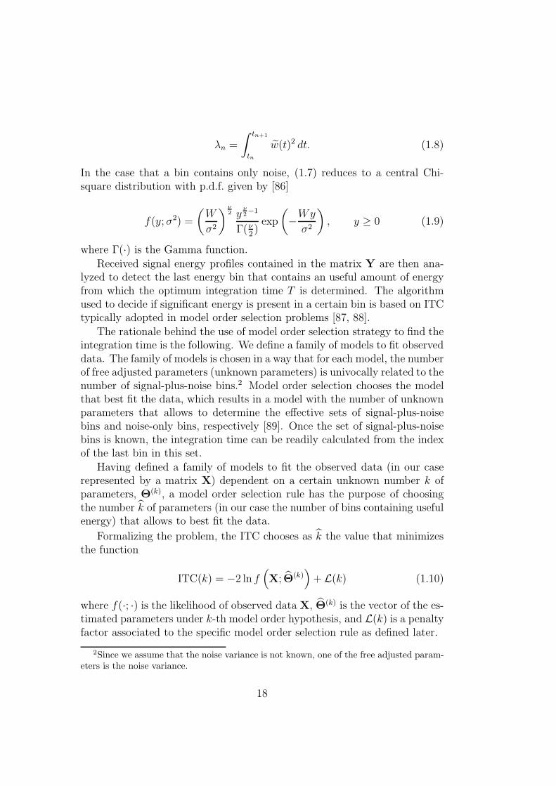
In the case that a bin contains only noise, (1.7) reduces to a central Chi-square distribution with p.d.f. given by [86]
f(y; σ2) =
(W
σ2
) ν2 y
ν2−1
Γ(ν2)exp
(−Wy
σ2
), y ≥ 0 (1.9)
where Γ(·) is the Gamma function.
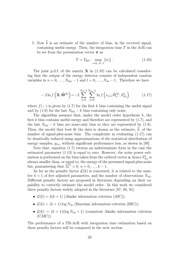
Received signal energy profiles contained in the matrix Y are then ana-lyzed to detect the last energy bin that contains an useful amount of energyfrom which the optimum integration time T is determined. The algorithmused to decide if significant energy is present in a certain bin is based on ITCtypically adopted in model order selection problems [87, 88].
The rationale behind the use of model order selection strategy to find theintegration time is the following. We define a family of models to fit observeddata. The family of models is chosen in a way that for each model, the numberof free adjusted parameters (unknown parameters) is univocally related to thenumber of signal-plus-noise bins.2 Model order selection chooses the modelthat best fit the data, which results in a model with the number of unknownparameters that allows to determine the effective sets of signal-plus-noisebins and noise-only bins, respectively [89]. Once the set of signal-plus-noisebins is known, the integration time can be readily calculated from the indexof the last bin in this set.
Having defined a family of models to fit the observed data (in our caserepresented by a matrix X) dependent on a certain unknown number k ofparameters, Θ(k), a model order selection rule has the purpose of choosingthe number k of parameters (in our case the number of bins containing usefulenergy) that allows to best fit the data.
Formalizing the problem, the ITC chooses as k the value that minimizesthe function
ITC(k) = −2 ln f(X; Θ(k)
)+ L(k) (1.10)
where f(·; ·) is the likelihood of observed data X, Θ(k) is the vector of the es-timated parameters under k-th model order hypothesis, and L(k) is a penaltyfactor associated to the specific model order selection rule as defined later.
2Since we assume that the noise variance is not known, one of the free adjusted param-eters is the noise variance.
18

In order to exploit this model order selection strategy for our problem,we proceed with an approach similar to that presented in [89] which can besummarized in the following steps.
1. Starting from the collected energy samples Y construct the vector d,adopted for unknown parameters estimation, by column averaging
dn =
Nob−1∑
l=0
yl,n , n = 0, . . . , Nbin − 1 . (1.11)
2. Sort the vector d in decreasing order obtaining z. We indicate with π =(π0, π1, . . . , πNbin−1) a vector of permutation indexes, so that zn = dπn
.Then, define the matrix of observed data, X, that contains the columnsof Y re-arranged according to the same ordering, that is, xl,n = yl,πn
.
3. In the k-th model order hypothesis, perform estimation of the param-eters vector
Θ(k) =(λ(k)0 , . . . , λ
(k)k−1︸ ︷︷ ︸
k bins with energy
, 0, . . . . . . . . . . . . , 0︸ ︷︷ ︸Nbin−k noise-only bins
, σ2(k)
)(1.12)
where3
λ(k)n =
(zn −
νσ2(k)
2W
)+, n = 0, . . . , k − 1 , (1.13)
is the non-centrality parameter estimate (i.e., signal energy estimate) ofthe n-th ordered bin, and σ2
(k) is the maximum likelihood (ML) estimate
of noise power σ2, that is,
σ2(k) =
1
TED
∑Nbin−1q=k zq
Nbin − k. (1.14)
4. Evaluate ITC(k) for k = 1, . . . , Nbin − 1 and take as k the value of kwhich minimize (1.10), that is
k = argmink∈{1,..,Nbin−1}
ITC(k) (1.15)
3The operator (x)+ stands for the positive part of x, that is (x)+ = max(0, x). Notethat the maximum likelihood (ML) estimator of the non-centrality parameter of a Chi-square r.v. cannot be expressed in closed-form. However, in [90] it is shown that (1.13) isa good approximation of the ML estimate when ν > 1.
19
5. Now k is an estimate of the number of bins, in the received signal,containing useful energy. Then, the integration time T in the AcR canbe set from the permutation vector π as
T = TED · maxi=0...k−1
{πi} . (1.16)
The joint p.d.f. of the matrix X in (1.10) can be calculated consider-ing that the output of the energy detector consists of independent randomvariables in n = 0, . . . , Nbin − 1 and l = 0, . . . , Nob − 1 . Therefore we have
− 2 ln f(X; Θ(k)
)=−2
Nob−1∑
l=0
Nbin−1∑
n=0
ln f(xl,n; Θ
(k)n , σ2
(k)
)(1.17)
where f(·; ·) is given by (1.7) for the first k bins containing the useful signaland by (1.9) for the last Nbin − k bins containing only noise.
The algorithm assumes that, under the model order hypothesis k, thefirst k bins contains useful energy and therefore are represented by (1.7), andthe last Nbin − k bins are noise-only bins so they are represented by (1.9).
Then, the model that best fit the data is chosen as the estimate, k, of thenumber of signal-plus-noise bins. The complexity in evaluating (1.17) canbe drastically reduced using approximations of the statistical distribution ofenergy samples, yl,n, without significant performance loss, as shown in [89].
Note that, equation (1.7) returns an indeterminate form in the case theestimated parameter (1.13) is equal to zero. However, the noise power esti-mation is performed on the bins taken from the ordered vector z, hence σ2
(k) isalways smaller than, or equal to, the energy of the presumed signal-plus-noisebin, guaranteeing that λ
(k)n > 0, n = 0, . . . , k − 1.
As far as the penalty factor L(k) is concerned, it is related to the num-ber k + 1 of free adjusted parameters, and the number of observations Nob.Different penalty factors are proposed in literature depending on their ca-pability to correctly estimate the model order. In this work we consideredthree penalty factors widely adopted in the literature [87, 88, 91]:
• L(k) = 2(k + 1) (Akaike information criterion (AIC));
• L(k) = (k + 1) logNob (Bayesian information criterion (BIC));
• L(k) = (k + 1)(logNob + 1) (consistent Akaike information criterion(CAIC)).
The performance of a TR-AcR with integration time estimation based onthese penalty factors will be compared in the next section.
20
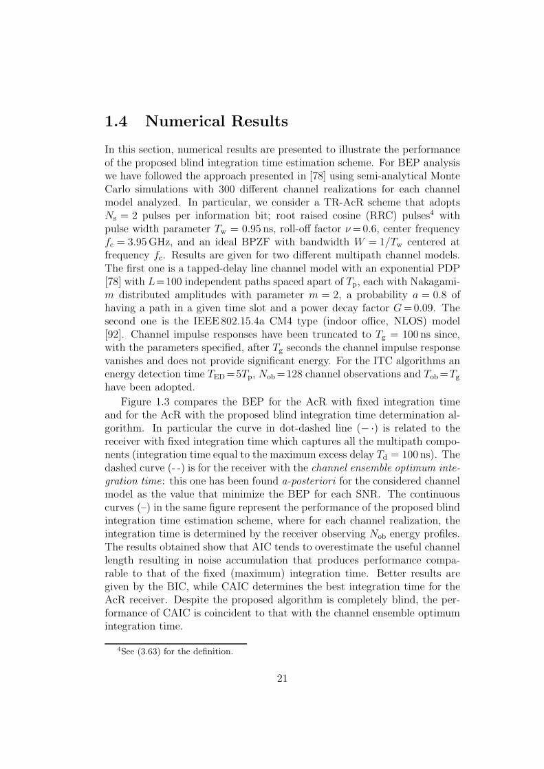
1.4 Numerical Results
In this section, numerical results are presented to illustrate the performanceof the proposed blind integration time estimation scheme. For BEP analysiswe have followed the approach presented in [78] using semi-analytical MonteCarlo simulations with 300 different channel realizations for each channelmodel analyzed. In particular, we consider a TR-AcR scheme that adoptsNs = 2 pulses per information bit; root raised cosine (RRC) pulses4 withpulse width parameter Tw = 0.95 ns, roll-off factor ν=0.6, center frequencyfc = 3.95GHz, and an ideal BPZF with bandwidth W = 1/Tw centered atfrequency fc. Results are given for two different multipath channel models.The first one is a tapped-delay line channel model with an exponential PDP[78] with L=100 independent paths spaced apart of Tp, each with Nakagami-m distributed amplitudes with parameter m = 2, a probability a = 0.8 ofhaving a path in a given time slot and a power decay factor G=0.09. Thesecond one is the IEEE802.15.4a CM4 type (indoor office, NLOS) model[92]. Channel impulse responses have been truncated to Tg = 100 ns since,with the parameters specified, after Tg seconds the channel impulse responsevanishes and does not provide significant energy. For the ITC algorithms anenergy detection time TED=5Tp, Nob=128 channel observations and Tob=Tg
have been adopted.
Figure 1.3 compares the BEP for the AcR with fixed integration timeand for the AcR with the proposed blind integration time determination al-gorithm. In particular the curve in dot-dashed line (− ·) is related to thereceiver with fixed integration time which captures all the multipath compo-nents (integration time equal to the maximum excess delay Td = 100 ns). Thedashed curve (- -) is for the receiver with the channel ensemble optimum inte-gration time: this one has been found a-posteriori for the considered channelmodel as the value that minimize the BEP for each SNR. The continuouscurves (–) in the same figure represent the performance of the proposed blindintegration time estimation scheme, where for each channel realization, theintegration time is determined by the receiver observing Nob energy profiles.The results obtained show that AIC tends to overestimate the useful channellength resulting in noise accumulation that produces performance compa-rable to that of the fixed (maximum) integration time. Better results aregiven by the BIC, while CAIC determines the best integration time for theAcR receiver. Despite the proposed algorithm is completely blind, the per-formance of CAIC is coincident to that with the channel ensemble optimumintegration time.
4See (3.63) for the definition.
21

Figure 1.3: BEP for the TR AcR as a function of the SNR for exponential PDP channelmodel, considering different strategies for the integration time determination.
Figure 1.4: BEP for the TR AcR as a function of the SNR for IEEE 802.15.4aCM4 channelmodel, considering different strategies for the integration time determination.
22
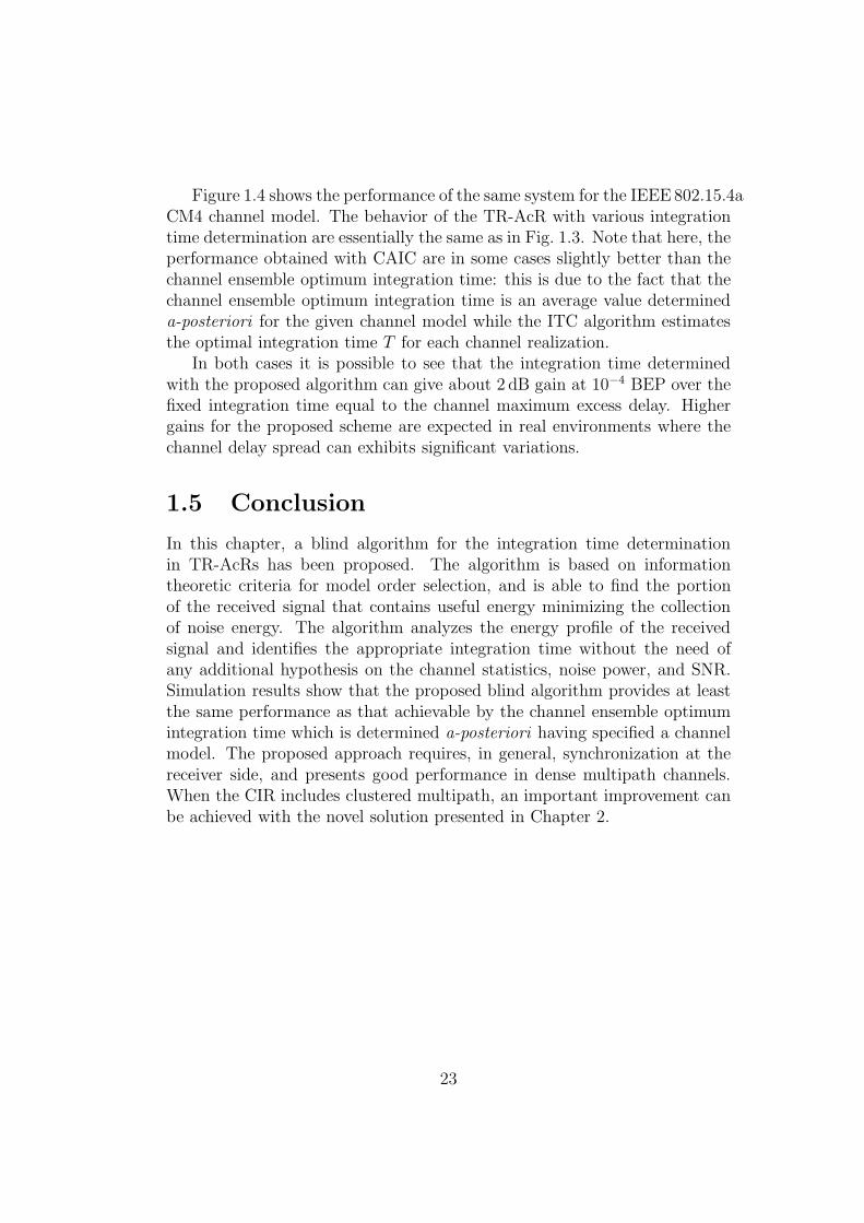
Figure 1.4 shows the performance of the same system for the IEEE802.15.4aCM4 channel model. The behavior of the TR-AcR with various integrationtime determination are essentially the same as in Fig. 1.3. Note that here, theperformance obtained with CAIC are in some cases slightly better than thechannel ensemble optimum integration time: this is due to the fact that thechannel ensemble optimum integration time is an average value determineda-posteriori for the given channel model while the ITC algorithm estimatesthe optimal integration time T for each channel realization.
In both cases it is possible to see that the integration time determinedwith the proposed algorithm can give about 2 dB gain at 10−4 BEP over thefixed integration time equal to the channel maximum excess delay. Highergains for the proposed scheme are expected in real environments where thechannel delay spread can exhibits significant variations.
1.5 Conclusion
In this chapter, a blind algorithm for the integration time determinationin TR-AcRs has been proposed. The algorithm is based on informationtheoretic criteria for model order selection, and is able to find the portionof the received signal that contains useful energy minimizing the collectionof noise energy. The algorithm analyzes the energy profile of the receivedsignal and identifies the appropriate integration time without the need ofany additional hypothesis on the channel statistics, noise power, and SNR.Simulation results show that the proposed blind algorithm provides at leastthe same performance as that achievable by the channel ensemble optimumintegration time which is determined a-posteriori having specified a channelmodel. The proposed approach requires, in general, synchronization at thereceiver side, and presents good performance in dense multipath channels.When the CIR includes clustered multipath, an important improvement canbe achieved with the novel solution presented in Chapter 2.
23

24

Chapter 2
Stop-and-Go Receivers
2.1 Motivations
In Chapter 1 it has been shown how the integration time T plays a fundamen-tal role on the performance achievable by non-coherent UWB demodulationschemes, as well known from the literature [25, 82, 79, 80, 81, 85, 83, 84, 93].However, when the channel PDP involves multipath clusters, the collectionof excessive noise is unavoidable regardless of the choice of T since a certainamount of the integrated signal is composed of noise only. In order to enhancethe effective SNR of non-coherent receivers, different weighting strategy havebeen proposed for both AcRs and EDRs [94, 95, 96, 97, 98, 99], based onassigning small weights to those portions of the received signal containing asmall amount of multipath energy. The main drawback of these techniquesis the need of a-priori channel knowledge or a potentially complex weightsselection procedure that requires parameters estimation and functions mini-mization at the receiver.
In this chapter, a low complexity strategy, based on the work [100] andcapable of alleviating excessive noise accumulation, for non-coherent UWBdemodulation is introduced. The proposed stop-and-go (SaG) scheme allowsthe AcR and the EDR to stop integrating whenever there is no significantsignal energy present in the channel output. The main advantages of theproposed scheme over conventional AcR and EDR are:
• The maximum integration time T can be kept as large as possible (e.g.,equal to the maximum expected channel excess delay) without noisepenalty;
• No a-priori channel information is required to optimize the perfor-mance;
25

• Better performance than conventional TR-AcR and EDR, even whenadopting integration time optimization, in the presence of clusteredmultipath.
The analysis is here carried out considering the classical TR-binary pulseamplitude modulation (BPAM) implementation with the reference and datapulses separated in time domain when adopting the AcR, and binary pulseposition modulation (BPPM) when adopting the EDR: however the proposedscheme can be applied to different non-coherent UWB demodulators anddifferent signaling formats such as code-multiplexed TR [76], OOK-EDR orM-PPM-EDR [60].
The remainder of the chapter is organized as follows. In Sec. 2.2, thesystem and the channel model are introduced. In Sec. 2.3, the proposedscheme is described. In Sec. 2.4, performance in terms of BEP for bothAcR with TR BPAM and EDR with BPPM are analyzed. The samplingexpansion approach originally proposed in [101] is adopted to analyze theSaG receiver schemes. In particular a semi-analytical method to evaluatethe BEP of the SaG exploitable for any kind of multipath channel is derived.Section 2.5 shows different strategies to optimize the performance of theproposed SaG receivers. Numerical results are presented in Sec. 2.6 to showthe performance gain of the SaG receivers in comparison with a classical AcRor EDR. Finally, a conclusion is given in Sec. 2.7.
2.2 Signal and Channel Model
2.2.1 TR-BPAM
In TR-BPAM signaling, the transmitted signal for a generic user1 can bedecomposed into a reference signal block br(t) and a data modulated signalblock bd(t). The band-pass transmitted signal is given by
sTR(t) =∑
i
br(t− iTs) + dibd(t− iTs) (2.1)
where Ts=NsTTRf is the symbol time, with TTR
f the average pulse repetitionperiod, di ∈ {−1, 1} the ith data symbol, and where Ns/2 is the number oftransmitted signal pulses in each block [69, 102, 70]. The reference signal
1Without loss of generality we focus on a single user system to simplify the mathemat-ical notation.
26

and the modulated signal blocks can be written as2
br(t) =
Ns2−1∑
j=0
√ETR
p aj p(t− j2TTRf − cjTp) ,
bd(t) =
Ns2−1∑
j=0
√ETR
p aj p(t− j2TTRf − cjTp − Tr) (2.2)
where p(t) is the normalized band-pass signal pulse with duration Tp, centerfrequency fc and unit energy. The energy of the transmitted pulse is thenETR
p = ETRs /Ns, where E
TRs is the symbol energy associated with TR signal-
ing. In the case of binary signaling that we are considering, the symbol energyequals the energy per bit, Eb. Note that the transmitted energy is equally al-located amongNs/2 reference pulses and Ns/2 modulated pulses. To enhancethe robustness of TR systems against interference and to allow multiple ac-cess, DS-SS and/or TH spread-spectrum techniques can be used as shown in(2.2). In case of DS-SS signaling
{aj}is the bipolar pseudo-random sequence
of the user. For the TH signaling{cj}is the pseudo-random TH sequence
related to the user, where cj is an integer in the range 0 ≤ cj < Nh, and Nh
is the maximum allowable integer shift. The duration of the received UWBpulse is Tg = Tp + Td, where Td is the maximum excess delay of the channel.To preclude ISI and isi, we assume that Tr ≥ Tg and NhTp+Tr ≤ 2TTR
f −Tg,where Tr is the time separation between each pair of data and referencepulses. We consider perfect synchronization at the receiver side although, asshown later, the proposed receiver is more robust to synchronization errorswith respect to conventional TR.3
2.2.2 BPPM
In this case, the transmitted signal can be expressed as
sBPPM(t) =∑
i
[(1 + di)
2b1(t− iTs) +
(1− di)
2b2(t− iTs))
](2.3)
where di ∈ {−1, 1} is the ith data symbol, Ts =Ns
2TEDf is the symbol duration
with Ns and TEDf denoting the number of pulses per symbol and the average
2Note that other combinations of data and reference pulses are also possible. Forsimplicity, and without loss of generality, we have adopted the conventional TR signaling,in which the number of reference and data pulses are equal[69].
3The sensitivity analysis to synchronization errors, however, is beyond the scope of thiswork. See, e.g., [103, 104].
27

pulse repetition period, respectively [73].4 The transmitted signal for di=+1and di=−1 can be written, respectively, as
b1(t) =
Ns2−1∑
j=0
√EED
p aj p(t− jTEDf − cjTp) ,
b2(t) =
Ns2−1∑
j=0
√EED
p aj p(t− jTEDf − cjTp −∆) (2.4)
where ∆ is the time shift between two different data symbols and the otherterms are defined as in (2.2). The energy of the transmitted pulse is EED
p =2EED
s /Ns, where EEDs is the symbol energy. Note that, adopting the posi-
tion modulation, the transmitted energy is allocated among Ns/2 modulatedpulses. To preclude ISI and isi we assume ∆ > Tg and NhTp+∆ ≤ TED
f −Tg.
2.2.3 Channel Model
The received signal can be written as rTR(t) = sTR(t) ⊗ h(t) + n(t) andrBPPM(t) = sBPPM(t)⊗h(t)+n(t) for TR-BPAM and for BPPM, respectively,where h(t) is the CIR and n(t) is zero-mean, additive white Gaussian noise(AWGN) with two-sided power spectral density (PSD) N0/2. We considerthe linear time-invariant channel model which CIR can be written as h(t) =∑L
l=1 αlδ(t − τl) where δ(·) is the Dirac-delta function, L is the number ofmultipath components, and αl and τl denote the amplitude and delay of thelth path, respectively [57].
2.3 Stop-and-Go Receivers
2.3.1 Conventional AcR
As shown in Fig. 2.1a, the conventional AcR first passes the received signalthrough an ideal band-pass filter with center frequency fc to eliminate out-of-band noise. If the bandwidth W of the filter is wide enough, then the signalpasses through undistorted, so ISI and isi caused by filtering is negligible.The received signal at the output of the band-pass filter is denoted by
rTR(t) =∑
i
br(t− iTs) + dibd(t− iTs)+n(t) (2.5)
4We set TTRf =
TEDf
2 so that the two signaling scheme present the same symbol duration.
28

r(t)
BPZF
r(t)
Tr
∫T
ZTR
(a)
r(t)
BPZF (·)2
∆∫T
∫T
ZED,1
ZED,2
(b)
Figure 2.1: Conventional non-coherent receivers. (a) AcR. (b) EDR.
where br(t) = br(t)⊗h(t)⊗hZF(t) and bd(t) = bd(t)⊗h(t)⊗hZF(t), hZF(t) is thefilter impulse response, and the term n(t) is a zero-mean, Gaussian randomprocess with autocorrelation function Rn(τ) = WN0 sinc(Wτ) cos(2πfcτ),with sinc(x) = sin(πx)/(πx). Note that, when |τ | is a multiple of 1/W , noisesamples are statistically independent, and when |τ | ≫ 1/W , that is, |τ | ≥ Tg,noise samples can be reasonably considered as statistically independent. Thefiltered received signal is passed through a correlator with integration intervalT , as shown in Fig. 2.1a. The incoming signal is correlated with a delayedversion of the reference signal, thus collecting the received signal energy.The integration interval T determines the number of multipath components(or equivalently, the amount of energy) captured by the receiver, as well asthe amount of noise energy accumulated. Hence, for the conventional TRsignaling, Tp ≤ T ≤ Tg.
Focusing on the data symbol at i=0, the decision statistic generated atthe AcR is then given by
ZTR =
Ns2−1∑
j=0
∫ j2TTRf +Tr+cjTp+T
j2TTRf +Tr+cjTp
rTR(t) rTR(t− Tr) dt . (2.6)
29

replacemen
r(t)
BPZF
r(t)
Tr
∫T
ZTR
DEC
(a)
r(t)
BPZF (·)2
∆∫T
∫T
ZED,1
ZED,2DEC
(b)
Figure 2.2: Stop-and-go receivers. (a) SaG-AcR. (b) SaG-EDR.
2.3.2 Conventional EDR
As shown in Fig. 2.1b, similarly to the AcR, the conventional EDR first passesthe received signal through an ideal band-pass filter with center frequencyfc to eliminate out-of-band noise. The received signal at the output of theband-pass filter can be written as
rBPPM(t) =∑
i
[(1 + di)
2b1(t− iTs) +
(1− di)
2b2(t− iTs)
]+n(t) (2.7)
where b1(t) = b1(t)⊗h(t)⊗hZF(t) and b2(t) = b2(t)⊗h(t)⊗hZF(t), and the otherterms are defined as in (2.5). The filtered received signal is passed througha couple of EDs, with integration interval T , that measure the energy intwo different time windows separated of ∆. As for the AcR, the integrationinterval T determines the number of multipath components captured by thereceiver, as well as the amount of noise energy accumulated.
Focusing on the data symbol at i = 0, the decision statistic generated at
30

Figure 2.3: Decision device (DEC).
the EDR is then given by
ZED =
Ns2−1∑
j=0
∫ jTEDf +cjTp+T
jTEDf +cjTp
(rBPPM(t))2 dt
︸ ︷︷ ︸ZED,1
−Ns2−1∑
j=0
∫ jTEDf +cjTp+T+∆
jTEDf +cjTp+∆
(rBPPM(t))2 dt
︸ ︷︷ ︸ZED,2
. (2.8)
2.3.3 SaG Receivers
As described earlier, the integration interval T of the conventional AcR andEDR must be suitably designed to avoid excessive noise energy accumulation,while capturing the maximum energy from the desired signal. However, inthe presence of clustered multipaths [105], an optimal choice of T may stilllead to excessive noise energy accumulation due to time gaps (inter-clusterintervals) in the received signal that do not contain useful energy. To alleviatethis problem, we propose the SaG-AcR shown in Fig. 2.2a and the SaG-EDRshown in Fig. 2.2b. The proposed SaG receivers include a decision device(DEC) composed of an ED (see Fig. 2.3) to detect which portions of thereceived signal contain useful energy. In particular, the idea is to decomposethe integration interval into Nbin short time slots (or bins) of duration TED=T/Nbin, and to select among them only those which contain significant energyfrom the desired signal. When no significant signal energy is detected in agiven bin, that bin is not used by the correlator in the SaG-AcR or notintegrated in the SaG-EDR, preventing noise energy accumulation.
The ED adopted for the decision regarding the bins to be integratedoperates on the delay path in the case of AcR, or in one of the two branchesof the EDR, when a training sequence is transmitted.5 We denote the energy
5In case of BPPM the receiver needs to operate in the specific time window where thesignal is effectively present, so the presence of a training sequence is assumed. Moreover,
31

samples at the output of the ED resulting from the jth received pulse with
Ej,n =
∫ tTRn
tTRn−1
r 2TR(t− Tr) dt, n = 1, 2, . . . , Nbin (2.9)
for the SaG-AcR, with tTRn = j2TTR
f + cjTp + Tr + nTED. In the case of SaG-EDR we consider that the energy samples adopted for the demodulation ofthe jth received pulse are collected on the previous data symbol that wesuppose part of the known training sequence, that is6
Ej,n =
∫ tEDn
tEDn−1
r 2BPPM(t− Ts) dt, n = 1, 2, . . . , Nbin (2.10)
with tEDn = jTEDf + cjTp + nTED.
The energy samples Ej,n are then used to select the desired bins throughthe variable uj,n which represents the state of the switch in the nth bin of thejth pulse. Such a variable is generated by the bin selection strategy as de-scribed in Section 2.5. Note that for the generic received pulse j, Nbin binarydecisions uj,1, . . . , uj,Nbin
are produced by the decision device. For notationalconvenience, in the following we will use the continuous-time switch signaluj(t) that commands the switching at the jth pulse defined as
uTRj (t) =
Nbin∑
n=1
uj,n rect
(t−tTR
n−1−TED/2
TED
)(2.11)
for the SaG-AcR, and
uEDj (t)=
Nbin∑
n=1
uj,n rect
(t−tEDn−1−TED/2
TED
)+
Nbin∑
n=1
uj,n rect
(t−tEDn−1−∆−TED/2
TED
)
(2.12)
for the SaG-EDR, where rect(t/TED) is a unit-amplitude rectangular pulsewith duration TED centered at the origin. The parameter TED determinesthe ability to separate time intervals containing paths from those containingnoise only. Small TED results in high temporal resolution but larger Nbin;hence, a trade-off between receiver performance and complexity is expected.
after a first phase, it is possible to operate with a decision-feedback approach, similarly towhat presented in [95].
6Without loss of generality we considerer a training sequence of all +1 so that thechannel response is concentrated in the first part each pulse repetition period is dividedin.
32
Note that with the SaG strategy the maximum integration time T can bekept as large as possible (e.g., equal to the maximum expected channel excessdelay) without noise penalty; moreover, in case of imperfect synchronization,noise-only bins preceding the signal TOA do not produce further penaltysince they are discarded by the switch driven by the decision device.
2.4 Performance Evaluation
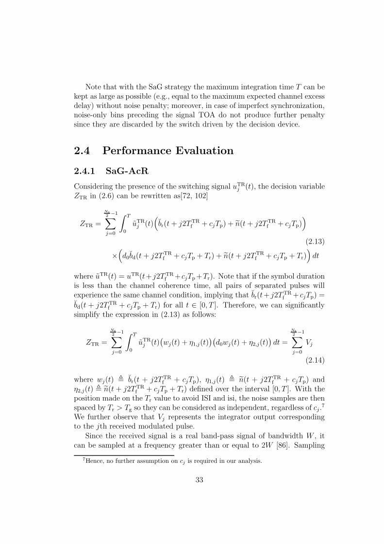
2.4.1 SaG-AcR
Considering the presence of the switching signal uTRj (t), the decision variable
ZTR in (2.6) can be rewritten as[72, 102]
ZTR =
Ns2−1∑
j=0
∫ T
0
uTRj (t)
(br(t+ j2TTR
f + cjTp) + n(t + j2TTRf + cjTp)
)
(2.13)
×(d0bd(t + j2TTR
f + cjTp + Tr) + n(t+ j2TTRf + cjTp + Tr)
)dt
where uTR(t) = uTR(t+ j2TTRf +cjTp+Tr). Note that if the symbol duration
is less than the channel coherence time, all pairs of separated pulses willexperience the same channel condition, implying that br(t+ j2TTR
f + cjTp) =
bd(t + j2TTRf + cjTp + Tr) for all t ∈ [0, T ]. Therefore, we can significantly
simplify the expression in (2.13) as follows:
ZTR =
Ns2−1∑
j=0
∫ T
0
uTRj (t)
(wj(t) + η1,j(t)
)(d0wj(t) + η2,j(t)
)dt =
Ns2−1∑
j=0
Vj
(2.14)
where wj(t) , br(t + j2TTRf + cjTp), η1,j(t) , n(t + j2TTR
f + cjTp) andη2,j(t) , n(t + j2TTR
f + cjTp + Tr) defined over the interval [0, T ]. With theposition made on the Tr value to avoid ISI and isi, the noise samples are thenspaced by Tr > Tg so they can be considered as independent, regardless of cj .
7
We further observe that Vj represents the integrator output correspondingto the jth received modulated pulse.
Since the received signal is a real band-pass signal of bandwidth W , itcan be sampled at a frequency greater than or equal to 2W [86]. Sampling
7Hence, no further assumption on cj is required in our analysis.
33

the received signal at rate 2W in the interval [0, T ] is then represented by2WT real samples.8 Following this approach, we can represent Vj as [72, 102]
Vj =1
2W
2WT∑
m=1
uTRj
( m
2W
)·(d0w
2j,m + wj,mη2,j,m + d0wj,mη1,j,m + η1,j,mη2,j,m
)
(2.15)
where the mth samples in the interval [0, T ] of wj(t), η1,j(t) and η2,j(t) in(2.14) are respectively denoted as wj,m, η1,j,m and η2,j,m. We can now express(2.15) conditioned on d0 and aj=+1 in the form of a summation of squares
Vj|d0=+1=2WT∑
m=1
uTRj
( m
2W
)[( 1√2W
wj,m + β1,j,m
)2
−β22,j,m
],
Vj|d0=−1=
2WT∑
m=1
uTRj
( m
2W
)[−(
1√2W
wj,m −β2,j,m
)2
+β21,j,m
](2.16)
where β1,j,m = 12√2W
(η2,j,m + η1,j,m) and β2,j,m = 12√2W
(η2,j,m − η1,j,m) are
statistically independent Gaussian r.v.s with variance N0/4. Due to thestatistical symmetry in (2.16) of Vj with respect to d0 and {aj}, we simplyneed to calculate the BEP conditioned on d0=+1 and aj=+1. For notationalsimplicity, we define the normalized r.v.s YTR,1, YTR,2, YTR,3, and YTR,4 as
YTR,1 =2
N0
Ns2−1∑
j=0
2WT∑
m=1
uTRj
( m
2W
)·(
1√2W
wj,m + β1,j,m
)2
,
YTR,2 =2
N0
Ns2−1∑
j=0
2WT∑
m=1
uTRj
( m
2W
)· β2
2,j,m ,
YTR,3 =2
N0
Ns2−1∑
j=0
2WT∑
m=1
uTRj
( m
2W
)·(
1√2W
wj,m − β2,j,m
)2
,
YTR,4 =2
N0
Ns2−1∑
j=0
2WT∑
m=1
uTRj
( m
2W
)· β2
1,j,m . (2.17)
Notice that in the summation, uTRj
(m2W
)∈ {0, 1} and accounts for the inclu-
sion of the mth sample resulting from the ED decision. It is thus convenient
8For convenience it is assumed that 2WT is an integer.
34

to define
NTRu =
Ns2−1∑
j=0
2WT∑
m=1
uTRj
( m
2W
)≤ NsWT (2.18)
as the total number of signal samples accumulated during T , related to asymbol.
Conditioned on the channel, YTR,1 and YTR,3 are non-central Chi-squarer.v.s with NTR
u degrees of freedom, whereas YTR,2 and YTR,4 are central Chi-square r.v.s with the same degrees of freedom as YTR,1 and YTR,3. Both YTR,1
and YTR,3 have the same non-centrality parameter 2γTR, where
γTR =1
N0
Ns2−1∑
j=0
2WT∑
m=1
uTRj
( m
2W
)· w
2j,m
2W=
1
N0
Ns2−1∑
j=0
∫ T
0
uTRj (t) · w2
j (t) dt
(2.19)
which, according to (2.11), can be rewritten as
γTR =1
N0
Ns2−1∑
j=0
Nbin∑
n=1
uj,n λTRj,n (2.20)
where
λTRj,n =
∫ nTED
(n−1)TED
w2j (t) dt, n = 1, 2, . . . , Nbin (2.21)
represents the energy of the noise-free received waveform in the nth bin. Also,(2.20) suggests that the non-centrality parameter is proportional to the ac-cumulated energy from selected bins (where selection is operated by uj,n) ofthe Ns/2 received modulated pulses that form a symbol. More precisely, theparameter γTR represents the instantaneous SNR obtained by accumulatingthe energy from a fraction of the received signal bins, hence named accumu-lated signal-to-noise ratio (ASNR). In fact, γTR is in general different fromthe SNR measured at the input of the AcR, due to the possible suppressionof certain paths by the bin selection strategy.
The p.d.f.s of YTR,1, conditioned on γTR, and YTR,2 are then given byfYTR,1|γTR(y1) = fNC(y1, 2γ
TR, NTRu /2) and fYTR,2
(y2) = fC(y2, NTRu /2) where
fNC(y, µ, ν) = e−(y+µ)
(y
µ
)(ν−1)2
Iν−1(2√yµ) , y ≥ 0 , (2.22)
fC(y, ν) =y(ν−1)
Γ(ν)e−y , y≥0 (2.23)
35

with Iκ(·) the κth order modified Bessel function of the first kind [106, ch.9, p. 374] and Γ(·) the Gamma function [106, ch. 6, p. 255].
Using the approach presented in [72, 102], the BEP of TR signaling withSaG-AcR conditioned on the single CIR realization and the decisions uj,n isgiven by P {YTR,1 < YTR,2|d0 = +1}. Thus, after some mathematical deriva-tions, the BEP can be expressed in the closed-form Pe,TR = Pe(γ
TR, NTRu ),
where9
Pe(γ,Nu) =e−γ
2Nu2
Nu2
−1∑
i=0
γi
i!
Nu2
−1∑
k=i
1
2k(k +Nu/2− 1)!
(k − i)!(Nu/2 + i− 1)!. (2.24)
2.4.2 SaG-EDR
Considering the presence of the switching signal uEDj (t), the decision variable
ZED in (2.8) can be rewritten as [73]10
ZED =
Ns2−1∑
j=0
∫ T
0
uEDj (t)
((1 + d0)
2b1(t+jTED
f +cjTp) + n(t+jTEDf +cjTp)
)2
dt
−Ns2−1∑
j=0
∫ T
0
uEDj (t)
((1− d0)
2b2(t+jTED
f +cjTp+∆)+n(t+jTEDf +cjTp+∆)
)2
dt
(2.25)
where uED(t) = uED(t+ jTEDf + cjTp). We can now rewrite (2.25) as follows:
ZED =
Ns2−1∑
j=0
∫ T
0
uEDj (t)
((1 + d0)
2w1,j(t) + η1,j(t)
)2
dt
︸ ︷︷ ︸Vj,1
−Ns2−1∑
j=0
∫ T
0
uEDj (t)
((1− d0)
2w2,j(t) + η2,j(t)
)2
dt
︸ ︷︷ ︸Vj,2
=
Ns2−1∑
j=0
Vj,1 −Ns2−1∑
j=0
Vj,2
(2.26)
where w1,j(t) , b1(t + jTEDf + cjTp), w2,j(t) , b2(t + jTED
f + cjTp + ∆),η1,j(t) , n(t + jTED
f + cjTp) and η2,j(t) , n(t + jTEDf + cjTp + ∆) defined
over the interval [0, T ].
9See also Appendix 3.D for the derivation.10Note that
(uEDj (t)
)2= uED
j (t) and uEDj (t+∆) = uED
j (t) for t ∈ [0, T ].
36

Following the approach adopted for the SaG-AcR we can exploit thesampling expansion representing Vj,1 and Vj,2 as
Vj,1 =1
2W
2WT∑
m=1
uEDj
( m
2W
)·((1 + d0)
2w1,j,m + η1,j,m
)2
,
Vj,2 =1
2W
2WT∑
m=1
uEDj
( m
2W
)·((1− d0)
2w2,j,m + η2,j,m
)2
(2.27)
where the mth samples in the interval [0, T ] of w1,j(t), w2,j(t), η1,j(t) andη2,j(t) in (2.26) are respectively denoted as w1,j,m, w2,j,m, η1,j,m and η2,j,m.For mathematical convenience, we define the normalized r.v.s YED,1, YED,2,YED,3, and YED,4 as
YED,1 =1
N0
Ns2−1∑
j=0
Vj,1|d0=+1 =1
N0
Ns2−1∑
j=0
2WT∑
m=1
uEDj
( m
2W
)· (w1,j,m + η1,j,m)
2
2W,
YED,2 =1
N0
Ns2−1∑
j=0
Vj,2|d0=+1 =1
N0
Ns2−1∑
j=0
2WT∑
m=1
uEDj
( m
2W
)· η
22,j,m
2W,
YED,3 =1
N0
Ns2−1∑
j=0
Vj,1|d0=−1 =1
N0
Ns2−1∑
j=0
2WT∑
m=1
uEDj
( m
2W
)· η
21,j,m
2W,
YED,4 =1
N0
Ns2−1∑
j=0
Vj,2|d0=−1 =1
N0
Ns2−1∑
j=0
2WT∑
m=1
uEDj
( m
2W
)· (w2,j,m + η2,j,m)
2
2W.
(2.28)
Again, in the summation, uEDj
(m2W
)∈ {0, 1} and accounts for the inclusion
of the mth sample resulting from the ED decision. It is thus convenient todefine
NEDu =
Ns2−1∑
j=0
2WT∑
m=1
uEDj
( m
2W
)≤ NsWT (2.29)
as the total number of signal samples accumulated during T , related to asymbol.
Conditioned on the channel, YED,1 and YED,4 are non-central Chi-squarer.v.s with NED
u degrees of freedom, whereas YED,2 and YED,3 are central Chi-square r.v.s with the same degrees of freedom as YED,1 and YED,4. Since, giventhe channel h(t), w1,j(t) = w2,j(t) = wj(t) (i.e., w1,j,m = w2,j,m = wj,m), both
37

YED,1 and YED,4 have the same non-centrality parameter 2γED, where
γED =1
2N0
Ns2−1∑
j=0
2WT∑
m=1
uEDj
( m
2W
)· w
2j,m
2W=
1
2N0
Ns2−1∑
j=0
∫ T
0
uEDj (t) · w2
j (t) dt
(2.30)
which, according to (2.12), can be rewritten as
γED =1
2N0
Ns2−1∑
j=0
Nbin∑
n=1
uj,n λEDj,n (2.31)
where
λEDj,n =
∫ nTED
(n−1)TED
w2j (t) dt, n = 1, 2, . . . , Nbin (2.32)
represents the energy of the noise-free received waveform in the nth bin. Asfor the SaG-AcR, the parameter γED is the ASNR.
The BEP of the SaG-EDR, conditioned on the single CIR realizationand the decisions uj,n, is then given by P {YED,1 < YED,2|d0 = +1}. SinceETR
p = 12EED
p , we have that λTRj,n = 1
2λEDj,n , so γTR = γED, fixed the CIR
realization and the decisions uj,n (i.e., the same ASNR and NTRu = NED
u ).Hence the the BEP of the EDR with BPPM Pe,ED = Pe(γ
ED, NEDu ), where
Pe(γ,Nu) is given by (2.24), equals the BEP of the SaG-AcR with TR-BPAMas for conventional AcR and EDR [107, 73, 60]. For this reason in the restof the chapter we will refer generically to γ and Nu.
In Fig. 2.4, the conditional BEP is plotted as a function of γ for differ-ent values of Nu. Fixing the amount of energy captured, or equivalently theASNR, the performance is worse for dispersive channels that have a longimpulse response. In fact, a long CIR implies a high Nu and consequentlymore noise is accumulated, as expected in a non-coherent scheme. To ob-tain the BEP of the SaG receivers, (2.24) can be used in a semi-analyticalMonte-Carlo approach that requires the generation of the CIR only and theevaluation of Nu and γ based on the bin selection strategies described in thefollowing section.
2.5 Bin Selection Strategies for the SaG Re-
ceivers
The analysis of the SaG receivers has shown how the performance is related tothe number of accumulated samples Nu and to the ASNR γ, both dependent
38

0 2 4 6 8 10 12 14 16 18 20γ [dB]
10-6
10-5
10-4
10-3
10-2
10-1
100
Bit
Err
or P
roba
bilit
yNu=2
Nu=20
Nu=200
Figure 2.4: Conditional BEP of the SaG receiver as a function of the ASNR for differentnumber of samples accumulated Nu.
on the bin selection strategy. To perform bin selection related to the jthpair of pulses, we consider the observation of Na previous reference pulsesfor the SaG-AcR, or Na pulses in the training sequence for SaG-EDR,11
collecting the energy samples Ej,n, Ej−1,n, . . . , Ej−Na+1,n for n = 1, . . . , Nbin.Without loss of generality and to simplify the notation, in the rest of thechapter we suppress the index j, and we define Eq,n = Ej−q+1,n with q =1, . . . , Na and n = 1, . . . , Nbin. Moreover, for notational convenience, let usarrange the energy samples Eq,n in a Na×Nbin matrix E and define the vectorε = (ε1, . . . , εNbin
) obtained by accumulation of Na previous energy samples,where the nth element of the vector is computed as12
εn =1
Na
Na∑
q=1
Eq,n n = 1, . . . , Nbin . (2.33)
Since it is advantageous to start collecting energy from bins with the higherenergy (and thus most probably those containing the useful signal), we definea vector ε′ = (ε′1, . . . , ε
′Nbin
) obtained by sorting ε in decreasing order. Inparticular, indicating with π = (π1, π2, ..., πNbin
) the vector of permutationindexes to sort ε in decreasing order, we have ε′n = επn
. Similarly, we denote
11Provided that the CIR remains constant during the time interval 2Na TTRf for the
SaG-AcR, and Na TEDf for the SaG-EDR, so that λTR
j,n = λTRn and λED
j,n = λEDn , ∀j.
12This corresponds to column averaging of E.
39

with λ′ the ordered version of the vector λ = (λ1, . . . , λNbin), with elements
λ′n = λπn
defined in (2.21) and (2.32) , and unknown at the receiver.13 Theirestimation can be performed having in mind that λn is the non-centralityparameter of the Chi-square distributed r.v. Eq,n [86, 89]. Unfortunately, theML estimator of the non-centrality parameter of a Chi-square r.v. cannot beexpressed in closed-form [90].14 Thus, instead of the ML, we use the simplerestimator [90]15
λ′n =
(ε′n − σ2TED
)+(2.34)
with σ2 = N0W .
2.5.1 Threshold-Based Bin Selection Strategy
A simple way to implement a bin selection strategy is to compare each sam-ple εn with a threshold, to make a binary decision regarding the presence ofsignificant useful energy. Intuitively, and in accordance to numerical results,there is an optimum threshold that minimizes the BEP. In fact, if the thresh-old is zero, all energy samples collected are used in the demodulation processand the scheme is equivalent to conventional AcR or EDR. Conversely, ifthe threshold is too high, only very few samples contribute to the demodula-tion process resulting in a drastic reduction of the ASNR. Therefore, in thissection we analyze the problem of designing a proper threshold for the SaGreceivers, proposing various schemes with different complexities and perfor-mance. In a threshold-based SaG receiver the bin selection strategy outputis the variable un which represents the state of the switch in the nth bin (ofthe jth pulse), according to the following rule
un =
{1, if εn > ξ ,0, otherwise
(2.35)
where ξ represents the threshold. Due to noise averaging in (2.33), morereliable decisions un are expected increasing Na.
Optimum Threshold
To find the optimum threshold (OT), which guarantees minimum BEP, wecalculate the corresponding number of bins to be collected, by analyzing
13Here λn refers indistinctly to λTRn or λED
n .14The maximization of the likelihood function leads to a numerical solution of an equa-
tion involving modified Bessel functions.15The operator (x)+ stands for the positive part of x, that is (x)+ = max(0, x). In [90] it
has been shown that the ML estimate is dominated by the simplified estimator (2.34) withsquared error as the loss function. As will be shown in Section 2.6 such simple estimatorgives satisfactory results.
40

the vector of ordered average energy samples ε′. In particular, since everycollected bin gives a contribution, in terms of accumulated samples, equalto NsWTED, the total number of samples collected by k bins is Nu
(k) =kNsWTED.
16 Considering the ordered vectors ε′ and λ′, the ASNR (2.20)or (2.31) corresponding to the selection of the first k ordered bins can berewritten as
γ(k) =Ns
2N0
k∑
n=1
λ′n (2.36)
for the SaG-AcR and
γ(k) =Ns
4N0
k∑
n=1
λ′n (2.37)
for SaG-EDR. Therefore, the optimum number of bins can be expressed as
k = argmink∈{1,...,Nbin}
Pe
(γ(k), Nu
(k))
(2.38)
where Pe(γ(k), Nu
(k)) is given by (2.24). Once k is calculated, the thresholdξ in (2.35) can be set as
ξ =ε′k+ ε′
k+1
2. (2.39)
Note that the minimum search in (2.38) can be stopped when the BEP startsincreasing since the energy samples are considered in decreasing order.17
This optimal approach for the threshold setting requires the knowledgeof the ASNR and the noise PSD N0. In general, γ(k) is not known a-prioritherefore it has to be estimated through (2.36) or (2.37) by substituting λ′
n
with λ′n calculated by (2.34). Similarly, if N0 is not known, it needs to be
estimated as explained in Section 2.5.1.
Approximate Optimum Threshold
Analyzing the properties of (2.24), it is possible to avoid its direct evaluationand minimization in (2.38) by an alternative solution which consists on thesearch for an approximate optimum threshold (AOT) through an iterativeapproach. For instance, suppose to perform the minimization (2.38) and to
16The notations A(k) and A(k) indicates that the quantity A refers to the case whereonly the first k out of Nbin bins with indexes π1, . . . , πk are selected.
17This leads to a function with only one absolute minimum.
41

be at step k having already collected the k − 1 strongest bins: if we addanother bin there is an increase of ∆Nu = NsWTED collected samples. Thisincrement is favorable only if the corresponding ASNR variation, indicatedwith ∆γ, is such that Pe(γ
(k−1) +∆γ,Nu(k−1) +∆Nu) < Pe(γ
(k−1), Nu(k−1)).
Since the increment ∆Nu depends only on receiver parameters (i.e., W andTED), it is possible to define the function
∆Pe(γ,∆γ,Nu)=Pe(γ+∆γ,Nu+∆Nu)−Pe(γ,Nu) (2.40)
which represents the variation of the BEP from step k to step k + 1. Thisfunction can be numerically inverted, by setting ∆Pe(γ,∆γ,Nu) = 0, findingthe ASNR variation ∆γ , g(γ,Nu) required to decrease the BEP. Theparticularity that leads us to this approach is the fact that g(γ,Nu) is, withgood approximation, not function of γ and Nu individually but of the ratioγ/Nu, that is, equivalently g(γNu, Nu) is only function of γ. To prove this,in Fig. 2.5 we shows the curves g(γNu, Nu) as a function of γ, varying Nu;in particular we consider Nu=10 (blue lines with ◦) and Nu=50 (red lineswith △), and different increments of the number of samples collected, thatis, ∆Nu = 2, ∆Nu = 4, ∆Nu = 8 and ∆Nu = 16. The figure confirms only avery weak dependence of g(γNu, Nu) fromNu, hence the above approximationappears reasonable. As further confirmed by numerical results in Section 2.6,such an approximation is more than satisfactory, especially for small ∆Nu.Therefore, for a given ∆Nu we define a new function, g(s) ≈ g(sNu, Nu),reflecting the approximation, where Nu is a fixed value,18 such that now∆γ ≈ g(γ/Nu). This function g(s) is so represented by the curves of Fig. 2.5substituting γ with s = γ/Nu in the horizontal axis.
Starting from these considerations it is possible to find the optimum num-ber of bins to be collected with the following iterative algorithm:19
k = 0repeatk = k + 1calculate ∆γ = γ(k) − γ(k−1)
until ∆γ < g(γ(k−1)/N
(k−1)u
)
set k = k − 1
where γ(k) is given by (2.36) or (2.37), depending on the receiver, and as-
suming γ(0)=0, N(0)u 6=0. Once found k the threshold ξ can be set according
to (2.39). As for the OT scheme it is necessary to estimate the ASNR and,the noise PSD.
18The value does not affect the result.19The function g(s) can be stored in a lookup table.
42

-20 -10 0 10 20-20
-10
0
10
Nu=10Nu=50
γ [dB]
∆γ[dB]
Figure 2.5: Required ASNR improvement ∆γ as function of the ASNR γ for different Nu.Continuous lines (–) are for ∆Nu = 2, dashed lines (- -) are for ∆Nu = 4, dot-dashed lines(· -) are for ∆Nu = 8, dotted lines (· ·) are for ∆Nu = 16.
Channel Ensemble Optimum Threshold
A third method for setting the threshold is based on the a-posteriori analysisof the average BEP, that is, averaged over several CIRs, as a function of thethreshold-to-noise ratio (TNR) TNR = ξ/N0. More precisely, we define thechannel ensemble optimum threshold (CEOT), as the one that minimizes theaverage BEP for each average SNR and for the considered channel model.Such definition is motivated by the numerical results in Section 2.6 showingthat the TNR giving the minimum average BEP for the SaG receivers hasa weak dependence on the channel model and on the SNR. Therefore, bythe use of such curves, it is possible to derive the optimum TNR and conse-quently the CEOT, once the noise PSD is known. Note that, such thresholdis fixed for a given channel and average SNR, and does not guarantee optimalperformance for each channel response realization as the OT presented in Sec-tion 2.5.1 or the AOT search in Section 2.5.1, but it produces the minimumBEP on average over the channel ensemble. The advantage is that once theoptimal TNR is known, it does not need any further calculation unless thesystem parameters are changed, leading to a rather simple implementation.
43

Noise Power Estimation
All threshold-based proposed SaG receivers require noise power knowledge,hence if N0 is not known a-priori, it must be estimated. A simple method toperform noise power estimation is to consider the average energy of the lastk bins taken from the vector ε′ of ordered energy samples, that likely containnoise only. In this manner the estimator for N0 is given by
N0 =
∑Nbin
n=k+1ε′n(
Nbin− k)WTED
. (2.41)
Obviously the estimation accuracy is related to k, Na and availability ofat least k noise-only bins. Therefore, the parameter k needs to be chosencarefully to avoid the presence of signal-plus-noise bins in the last k elementsof ε′. Such information requires in general some a-priori knowledge of theCIR duration. If not available, the blind bin selection strategy described inthe next section can represent a very robust and viable solution.
2.5.2 Blind Bin Selection Strategy
To derive a bin selection strategy that does not require any a-priori knowl-edge about the ASNR and the noise PSD, and does not need to set-up athreshold, we propose an approach based on ITC for model order selectionproblems [108, 87, 109, 88]. The key idea is the same as the one alreadypresented for the integration time determination problem in Sec.1.3, andinvolves determining the bins containing noise only by using model orderselection methods. In this way, the decision device in Fig. 2.3 acts as a non-linear excision filter, which allows the deletion of the noise-only bins [89, 110].In particular, we define a family of models to fit the observed data E . Thefamily of models is defined in a way that for each model, the number of freeadjusted parameters is equal to the number of signal-plus-noise bins. Withmodel order selection we then choose the model that best fits the data, whichcorresponds to the model with the number of free adjusted parameters equalto the actual number of signal-plus-noise bins. Once the bins containing thedesired signal are detected, noise-only bins can be deleted by the switch.
Formalizing the problem, the ITC chooses as k the value that minimizesthe function [87]
ITC(k) = −2 ln f(E ; Θ(k)
)+ L(k) (2.42)
where f(·; ·) is the likelihood function of observed data E conditioned on the
vector of estimated parameters, Θ(k), under model order hypothesis k, and
44

L(k) is a penalty term that depends on the specific model order selectionrule as shown later.
To exploit the model order selection strategy (2.42) the p.d.f.s of ther.v.s representing the observations is required. The energy sample Eq,n at theoutput of the ED is a non-central Chi-square distributed r.v. whose p.d.f. is[86, 111]
fS(ε;λn, σ2) =
W
σ2fNC
(W
σ2ε,W
σ2λn, ν
), ε ≥ 0 (2.43)
with ν = 2WTED degrees of freedom.20 For those bins containing noise only,(2.43) reduces to a central Chi-square distribution with p.d.f. [86, 111]
fN(ε; σ2) =
(W
σ2
)ν2
fC
(W
σ2ε, ν
), ε ≥ 0 . (2.44)
In the k-th model order hypothesis the parameter vector is
Θ(k) =(λ′(k)
1 , . . . . . . , λ′(k)k︸ ︷︷ ︸
k signal-plus-noise bins
, 0, . . . . . . . . . . . . , 0︸ ︷︷ ︸Nbin−k noise-only bins
, σ2(k)
)(2.45)
where λ′(k)n > 0 represents the non-centrality parameter estimate, obtained
by (2.34) where σ2 is replaced by its ML estimate, σ2(k), under the hypothesis
of having Nbin − k noise-only bins, that is
σ2(k) =
1
TED
∑Nbin
n=k+1 ε′n
Nbin − k. (2.46)
Then,
k = argmink∈{1,...,Nbin}
ITC(k) (2.47)
and the corresponding switch state to allow deletion of noise-only bins duringsymbol detection is uπn
= 1 for n = 1, . . . , k and uπn= 0 elsewhere.
The joint p.d.f. of the matrix E in (2.42) can be calculated consideringthat the output of the energy detector produces independent random vari-ables in q=1, . . . , Na and k=1, . . . , Nbin [89]. Therefore, the log-likelihood
20For convenience it is assumed that 2WTED is an integer.
45

function of observed data becomes21
ln f(E ; Θ(k)
)=
Na∑
q=1
[k∑
n=1
ln fS
(Eq,πn
; Θ(k)n , σ2
(k)
)+
Nbin∑
n=k+1
ln fN(Eq,πn
; σ2(k)
)].
(2.48)
Finally, the term L(k) in (2.42) is a penalty term which has differentexpressions according to the model order selection rule. For the AIC [108, 91]it is L(k) = 2(k + 1), since k + 1 is the number of parameters under thehypothesis k (k non-centrality parameters for the k signal-plus-noise bins,plus the noise variance σ2
(k)). For the BIC [112] it is L(k) = (k + 1) logNa.
2.6 Numerical Results
In this section, we compare the SaG receivers with the conventional AcR andEDR. In particular, we consider Ns = 2 and transmitted pulses compliantwith the IEEE 802.15.4a standard [113]: RRC pulses22 with pulse width pa-rameter Tw = 1ns,23 roll-off factor ν = 0.6, center frequency fc = 4GHz areadopted. At the receiver, an ideal band-pass filter with bandwidthW =2GHzcentered at frequency fc is considered.
24 Performance analysis is proposedin the IEEE 802.15.4a multipath channel model [114] and, if not otherwisestated, the channel model CM1 is considered, with channel responses dura-tion truncated up to 150 ns. For both conventional AcR and EDR, and SaGreceivers we consider a time-bandwidth product WT =300, which guaranteesto capture the entire CIRs. The BEP, averaged on different channel realiza-tions, as function of the average SNR, is adopted as performance metric.
Figure 2.6 presents the averaged BEP of the proposed SaG receivers asfunction of Na considering the OT bin selection strategy (Section 2.5.1) withperfect knowledge of the noise power and of the non-centrality parameters
21Note that, because of the ordering imposed to the parameter vector λ′ (and as aconsequence on the non-centrality parameters in (2.45)) the column indexes in E arepermutated accordingly to π. Equation (2.43) returns an indeterminate form in the case
the non-centrality parameter estimate λ′(k)
n is equal to zero; this fact seems to occur sincewe adopt the estimator (2.34) that subtracts the average noise energy from each energysample. However the noise power estimation is performed on the last Nbin − k energysamples of ε′, hence σ2
(k) is always smaller than, or equal to, the energy of the signal-plus-
noise bins, guaranteeing that λ′(k)
n > 0 for n = 1, . . . , k.22See (3.63) for the definition.23The correspondent pulse duration is Tp ≈ 3Tw.24 The value of the receiving filter bandwidth W =2/Tw=2GHz ensures that the signal
spectrum of bandwidth (1 + β)Tw = 1.6GHz passes undistorted.
46
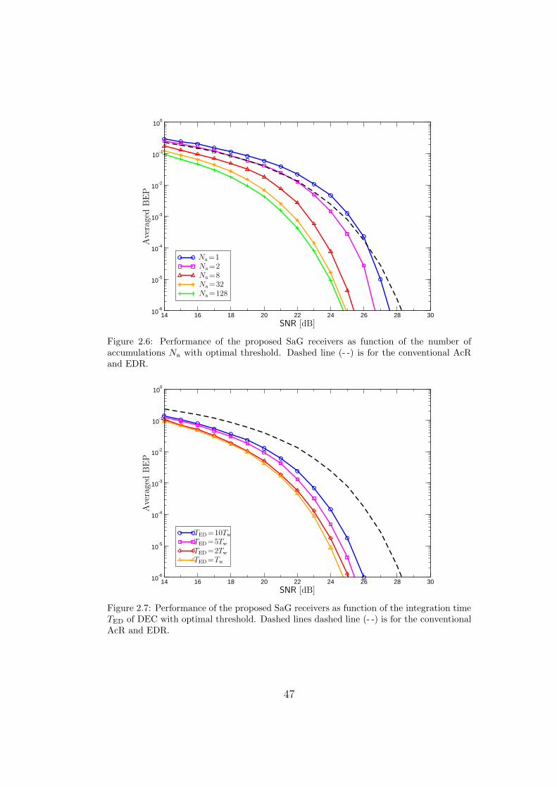
14 16 18 20 22 24 26 28 3010-6
10-5
10-4
10-3
10-2
10-1
100
Na=128Na=218Na=812Na=321Na=128
SNR [dB]
AveragedBEP
Figure 2.6: Performance of the proposed SaG receivers as function of the number ofaccumulations Na with optimal threshold. Dashed line (- -) is for the conventional AcRand EDR.
14 16 18 20 22 24 26 28 3010-6
10-5
10-4
10-3
10-2
10-1
100
TED=10Tw
TED=5Tw1TED=2Tw1TED=Tw1
SNR [dB]
AveragedBEP
Figure 2.7: Performance of the proposed SaG receivers as function of the integration timeTED of DEC with optimal threshold. Dashed lines dashed line (- -) is for the conventionalAcR and EDR.
47

14 16 18 20 22 24 26 28 3010-6
10-5
10-4
10-3
10-2
10-1
100
k=288k=108k=508N0 = N0
SNR [dB]
AveragedBEP
Figure 2.8: Performance of the proposed SaG-AcR for different number k of bins consideredfor noise PSD estimation. Continuous lines (–) are for the receiver with OT, dotted lines(· ·) are for the receiver with AOT. Dashed line (- -) is for the conventional AcR. Dot-dashed line (- ·) is for the prior knowledge of N0 and the non-centrality parameters λn
(ideal receiver).
λn (ideal receiver). An ED integration time TED = Tw is considered. Forcomparison, the performance of the conventional AcR is reported. The figureshows that the proposed scheme presents a gain of about 3−4 dB with respectto the conventional AcR if a proper number of accumulations on the energyprofile is adopted (e.g., Na > 8). In the following, a value Na = 128 isconsidered. The impact of a different ED integration time TED of DECis reported in Fig. 2.7. As expected, the best BEP is achieved for a TED
comparable to the pulse duration (TED = Tw), but significant gains are alsopresent for longer integration times with a consequent decrease of the receivercomplexity. In the following results we will assume TED=Tw.
We now focus the analysis on the effects of the different bin selectionstrategies. In the following we consider the SaG-AcR.25 Figure 2.8 presentsthe performance of the SaG-AcR with OT (in continuous lines), for different
number of bins k considered for noise PSD estimation operated by (2.41).
25It has been demonstrated that the BEP is the same for SaG-AcR and SaG-EDR.However, the EDR performs the bin selection with an effective SNR 3 dB higher than theAcR, due to the fact that ETR
p = 12E
EDp . The effective performance of the SaG-EDR is
then improved due to the possibility of taking more reliable decisions on the bins to beintegrated.
48

0 1 2 3 4 5 6 7 8 9 1010-6
10-5
10-4
10-3
10-2
10-1
100
SNR=20 dBSNR=22 dBSNR=24 dB
TNR [dB]
AveragedBEP
Figure 2.9: Performance of the proposed SaG-AcR with fixed threshold ξ as function ofTNR for different SNRs. Continuous lines (–) are for the CM1 channel model, dashedlines (- -) are for the CM5 channel model.
From the estimate N0, the non-centrality parameters λ′n are obtained by
(2.34). Comparison with the case of perfect noise PSD knowledge and esti-mation of λn, as well as perfect knowledge of both noise power and λn is alsoprovided. In the same plot the results obtained with AOT are also reported(in dotted lines). Regarding the AOT, given the adopted Ns, W and TED,we have ∆Nu=4 for the threshold calculation.26 A realistic implementationaccounting for a quantization step of 0.1 dB for s = γ/Nu in the lookup ta-
ble containing g(s) is considered. As we can see, increasing k decreases thevariance of noise power estimate with a corresponding performance improve-ment. The value k = 50 allows obtaining a performance almost comparableto the one of the receiver with perfect parameter knowledge at high SNR,while a loss of about 1 dB is present at medium SNR correspondent to aBEP of 10−3. It is important to remark that a significant gain is in any casepresent with respect to the conventional AcR, and the estimation of the non-centrality parameters λn adopting the simplified estimator (2.34) does notsignificantly worsen the performance. Moreover, the adoption of the AOT re-sults in a minimum performance loss with respect to the OT. It is importantto remark that in this case the threshold setting procedure is significantlysimplified.
26The curve corresponding to Nu=10 in Fig. 2.5 is adopted.
49

14 16 18 20 22 24 26 28 3010-6
10-5
10-4
10-3
10-2
10-1
100
k=288k=108k=508N0 = N0
SNR [dB]
AveragedBEP
Figure 2.10: Performance of the proposed SaG-AcR with fixed threshold TNR = 4dB fordifferent number k of bins considered for noise PSD estimation. Dashed line (- -) is for theconventional AcR.
We now consider on the CEOT described in Section 2.5.1. Figure 2.9shows the averaged BEP as function of the TNR for different average SNRsand considering the CM1 and the CM5 channel models. For high TNRs theperformance worsens as the bin selection reduces the amount of signal energyat the input of the integrator, while when the TNR is below 2 dB the perfor-mance is that of the conventional AcR. For the parameter TED considered,there is an optimum TNR value between 4 to 4.5 dB, which minimizes the av-eraged BEP irrespectively, with good approximation, of the SNR and channelmodel. Hence, it is possible to set-up a threshold that depends on N0 and thereceiver parameters, in particular the integration time TED. Adopting thisapproach the only estimation of N0 is necessary with a significant reductionof the receiver complexity.27 In Fig. 2.10, the averaged BEP of the proposedreceiver with TNR =4dB and that of the conventional AcR are reported as afunction of the number k of bins considered for noise power estimation. It isimportant to underline how in this case with k=10 only the performance issignificantly close to the one of the receiver with perfect noise power knowl-
27The value of TNR=4dB which results in a minimum BEP is also easily explainable:a noise-only bin has an average energy N0WTED, which corresponds to 2N0 since weconsidered TED=Tw and W =2/Tw, as a consequence the threshold ξ is just 1 dB abovethe average energy of noise bins, enough to remove noise-only bins and preserve signal-plus-noise bins.
50

14 16 18 20 22 24 26 28 3010-6
10-5
10-4
10-3
10-2
10-1
100
AICCIBICCIOTCSAOTCCEOT
SNR [dB]
AveragedBEP
Figure 2.11: Performance of the SaG-AcR with different bin selection strategies. Contin-uous lines (–) are for the blind selection strategy. Dotted lines (· ·) are for the threshold-
based strategies with k = 10. Dashed line (- -) is for the conventional AcR. Dot-dashedline (- ·) is for the SaG-AcR with optimum threshold and prior parameter knowledge (idealreceiver).
edge: this fact can be explained since adopting this threshold setting methodthe estimation of the non-centrality parameters λn operated starting from N0
is avoided, with a consequent prevention of estimation errors propagation.
Finally, the performance of the SaG-AcR receiver with the blind bin selec-tion strategy presented in Section 2.5.2, is reported in Fig. 2.11. For compari-son, the results regarding threshold-based bin selection strategies with k=10are reported. Analyzing the curves we can conclude that the AIC criterion isnot the best choice to properly select the bins, especially at high SNR: this ismainly due to the fact that AIC tends to overestimate the model order, thatis, the number of bins containing useful multipath energy, hence collectingenergy also from noise-only bins [87]. On the contrary the BIC is a consistentcriterion and for a sufficient number of observations, Na, it properly selectsthe signal-plus-noise bins. Adopting the BIC criterion the performance ofthe proposed receiver with blind selection strategy is very close to that ofthe receiver adopting the CEOT and the ideal receiver with OT and a-prioriparameters knowledge, and performs better than OT and AOT when noisepower and non-centrality parameters λn need to be estimated. It is interest-ing to remark despite the CEOT is optimal for the channel ensemble whilethe OT and AOT are optimized for (hence dependent on) each CIR, CEOT
51
performs better for intermediate SNRs. This behavior can be explained con-sidering that while CEOT requires only noise power estimation, OT and AOTneed also non-centrality parameters estimation, therefore CEOT results tobe more robust at low and medium SNRs, where estimation errors can berelevant.
2.7 Conclusion
In this chapter, novel AcR and EDR schemes for UWB BPAM-TR andBPPM, called SaG receivers have been introduced. They are based on energydetection, that avoid noise energy collection from those intervals of the re-ceived signal that do not contain useful energy. The proposed strategy is easyto implement and therefore is attractive for robust low-complexity commu-nication systems. First, a closed-form semi-analytical expression, which pro-vides insight into the impact of noise and energy collection on system perfor-mance has been derived. Starting from this, different bin selection strategieswith different complexities and performance have been investigated. Finally,the numerical comparison of the proposed receivers with the conventionalAcR and EDR and for different bin selection strategies highlights the perfor-mance gain that can be obtained adopting the SaG strategy, with a potentialextension of the benefits to other non-coherent UWB signaling techniques.
52

Part II
Time-Delay Estimation
53


Introduction
Time-delay estimation (TDE), also referred to as epoch estimation or TOAestimation, is a classical signal processing problem and a fundamental opera-tion in different context [115, 116, 117, 118, 119, 120, 121, 122, 51, 123]. TDEis necessary for timing digital receivers, audio processing and source localiza-tion [124, 125, 126] radar and sonar target distance estimation [127, 128, 129,130, 131], synchronization of wired or wireless systems [132, 133], and it isone of the functionalities enabling localization, key feature of context-awarewireless networks [134, 135, 51].
In fact, among different localization techniques, those based on distanceestimation (ranging) are more suitable for high localization accuracy.28 Start-ing from TOA measurements, that is starting from the knowledge of the prop-agation time between two devices, it is in fact possible to recover directly thedistance (i.e., the range) by simple multiplication for the speed of light. It iswell known that ranging accuracy is directly proportional to the signal band-width and hence the use of wideband or UWB signals is attractive for rangingapplications. In particular, UWB technology offers the potential of achievinghigh ranging accuracy even in harsh environments [51, 139, 134, 140, 138],due to its ability to resolve multipath [53, 54, 55]. Ranging techniques basedon TOA estimation of the first arriving signal path are mainly affected bynoise, multipath components, pulse distortion, obstacles, interference, andclock drift [141, 51, 134, 140, 142]. These problems, mainly due to the prop-agation environment, especially when indoor, pose several limitations on theachievable performance in terms of accuracy since the received signal has em-bedded some unknown parameters or, in the worst case, must be consideredalmost totally unknown. In these cases practical estimation techniques havebeen proposed. Unfortunately, the known bounds are very optimistic whencompared to the performance of these practical estimators [51].
The aim of this part is presenting some novel results on performancebounds for TDE when signals are partially known or unknown at the re-ceiver, with applications to the various contexts already remarked and witha particular emphasis on the problem of ranging for location determination.
28We refer the reader to [24, 52] for more information on the variety of localizationtechniques and to [136, 137, 138] for the fundamentals bounds.
55

56

Chapter 3
Bounds on Time-DelayEstimation for Partially Knownand Unknown Signals
3.1 Motivations
Several papers address the TOA estimation problem in the presence of mul-tipath such as [55, 59], where amplitudes and delays of the multipath compo-nents are jointly estimated using the ML approach [55, 59] or the generalizedML based technique analyzed in [143] (see for example the survey [51] andthe references therein).
Such kind of estimators rely on coherent correlation, that is, they as-sume local knowledge of the received pulse template, and offer in theorythe best performance. However their design and implementation is not al-ways practical for several reasons. In fact the waveform shape estimationmight be computationally intensive when signals are distorted by the chan-nel. Even with perfect knowledge of the waveform, especially adopting UWBsignals, pulse overlap due to multipath might result in strong signal distor-tion. In addition, the waveform could not be completely well specified atthe transmitter side due to random phase of the local oscillator, as will beclarified later. For these reasons a plethora of approaches with different lev-els of complexity and performance have been developed in the literature.Among them, of particular interest when dealing with low complexity re-ceivers and unknown waveforms, are those relying on energy measurements[144, 51, 145, 132, 146, 147, 148, 135, 149]. In many of these approachesthe energy of the received signal is evaluated in time slots with durationT comparable with the pulse duration. Several techniques are proposed to
57

identify the index of the time slot containing the first arriving signal com-ponents. Unfortunately one drawback of these approaches is that a floor onestimation mean squared error (MSE), equal to T 2/12, arises due to timediscretization.
Moreover, although energy detection is widely investigated both fromthe practical and from the theoretical point of view for the signal detectionproblem, especially when in presence of unknown deterministic signals [86,150, 151, 152, 153, 111, 154, 155, 156], a general lack of theoretical foundationis present for the TOA estimation problem, despite the broad application ofthe technique.
Besides specific TOA estimation algorithms, estimation error bounds playa fundamental role since they serve as useful performance benchmarks for thedesign of TOA estimators.
Cramer-Rao bound (CRB) has been widely used as a performance bench-mark for assessing the estimator error [157, 122, 158, 51, 159, 160]. Its use isjustified by asserting that the performance of the ML estimator approachesasymptotically to the CRB for sufficiently high SNRs [66]. It is well known,however, that the CRB is not accurate at low and moderate SNR. In fact,the performance of the TOA estimator, as all non-linear estimators, is char-acterized by the presence of distinct SNR regions (i.e., low, medium, andhigh SNRs) corresponding to different modes of operation. This behavior isreferred to as the threshold effect [161] and it has been studied in a varietyof contexts (e.g., [116, 162, 117, 163, 118, 119]). In a low SNR region (alsoknown as the a priori region), the MSE is close to that obtained solely fromthe a priori information about the TOA and signal observations provide littleadditional information. In a high SNR region (also known as the asymptoticregion), the MSE is accurately predicted by the CRB. Between these twoextremes, there may be an additional region (also known as the transition re-gion or ambiguity region) where observations are subject to ambiguities thatare not accounted for by the CRB [66].
Although CRB accurately predicts the MSE in asymptotic region, operat-ing conditions in such a region are often impractical due to the requirementson emitted power level typical in short-range systems. In addition, the CRBcannot be derived in certain conditions [66]. Therefore other bounds, whichare more complicated but tighter than the CRB, have been proposed inthe literature. In particular, the Barankin bound identifies the SNR values(thresholds) that distinguish the ambiguity region [164, 165]. The Ziv-Zakaibound (ZZB) [166], with its improved versions such as the Bellini-Tartarabound [167] and the Chazan-Zakai-Ziv bound [168], as well as the Weiss-Weinstein bound (WWB) [163] are more accurate than the Barakin bound.They can be applied to a wider range of SNRs and account for both ambiguity
58

effects and a priori information of the parameter to be estimated. However,they may not be analytically tractable in many cases or require more com-plicated evaluations compared to the CRB, especially when operating in thepresence of multipath [169, 170, 171, 172].
In [173] the expression of the CRB for multipath environments is givenstarting from the joint estimation of channel parameters. In [172] the ap-proach developed in [116, 162] for the estimation of the relative delay be-tween two sensors emitting noise-like signals is extended to that emittingUWB signals. The work [174] evaluates the ZZB for Gaussian signals assum-ing perfect channel knowledge at the receiver. A few results are present forthe case where the receiver has a partial or no knowledge about the channel[170, 171]. In particular, in [170] the ZZB using measured data as well asMonte Carlo generated CRs is investigated, whereas [171] derives the ZZBusing second order statistics approach by modeling the received signal asnon-stationary Gaussian random process.
The aim of this chapter is to investigate ZZBs on the MSE associatedwith the TOA estimation of partially known and unknown signals. Thesebounds represent the performance limits of any TOA estimator dealing withthe same hypothesis about signal knowledge. To allow for a comprehensiveoverview of the problems, some previous results are also revised and discussedwhen necessary.
The key contributions of the chapter can be summarized as follows:
• Derivation of the ZZB for TOA estimation for signals with unknownphase;
• Derivation of the ZZB for TOA estimation for unknown deterministicsignals;
• Comparison of the ZZBs and CRBs with the performance of the revisedand derived ML estimators under the same hypothesis on the signalknowledge.
The remainder of the chapter is organized as follows. In Sec. 3.2 thesignal and channel models are introduced. The ZZB is reviewed briefly inSec. 3.3. The bound is then derived in Sec. 3.4 and it is compared to theCRB in the ideal AWGN scenario. Section 3.5 extends the classical ZZBfor the case of partially known signals, in particular signals with unknowncarrier phase. Section 3.6 derives new fundamental bounds for the case ofunknown deterministic signals. For the derivations several tools such as seriesexpansion of signals are revised and extended to particular cases of interest inthe appendices. In Sec. 3.7 classical TOA estimators are reviewed considering
59

the results obtained during the derivation of the bounds. Numerical resultsare then presented in Sec. 3.8 providing a comparison between the boundsand the estimators performance.
3.2 Signal Model
We consider, as transmitted signal, a time-limited waveform p(t) with du-ration Tp. When p(t) has a bandpass nature, we denote by fc its centralfrequency and we refer, for convenience, to its ELP as p(t) so that
p(t) = ℜ{p(t) e2πfct
}. (3.1)
Bandpass signals are usually generated starting from in-phase and in-quadraturebaseband components pI(t) and pQ(t) that are further used as input to aquadrature modulator adopting a local oscillator with carrier frequency fcand initial phase φ, that is, p(t) = p0(t) e
φ, with p0(t) = pI(t) + pQ(t).Note that every physically realizable signal is time-limited, and hence,
rigorously, not limited in bandwidth. However, in practice, the signal band-width can be truncated to a suitable value W so that the energy contributionof out-of-band signal components is negligible. More rigorously, we considerp(t) band-limited at level ǫ with bandwidth W , if W is the smallest value forwhich1
∫
|f |>W
|P (f)|2 df < ǫ (3.2)
where P (f) is the Fourier transform of p(t) and the energy ǫ lying outsidethe frequency range is less than the smallest amount we are able to detectby any means in the real world [175].
Signal p(t) is transmitted through a channel and the received signal canbe expressed as
r(t) = s(t− τ) + n(t) (3.3)
where s(t) = p(t) ⊗ h(t) is the CR, h(t) is the CIR, τ is the TOA of thereceived signal to be estimated, and n(t) is AWGN with zero mean and two-sided spectral density N0/2 in the signal band of width W .2 We consider thedelay introduced by the channel de-embedded from h(t) and accounted forby τ . The duration of the received CR s(t) is Ts = Tp + Td, where Td is the
1When p(t) has a bandpass nature, the integration in (3.2) is performed over the interval|f | >
{fc +
W2
}∪{|f | < fc − W
2
}.
2We consider the presence of a zonal filter that removes all the noise components outsideW .
60

maximum excess delay of the channel. In the absence of other information, weassume the TOA τ to be unknown and randomly distributed in the interval[0, Ta]. The goal is to obtain the estimate τ of τ by observing r(t) in theinterval [0, Tob], with Tob > Ta + Ts, with partial (even statistical) or noknowledge on s(t) available.
For further convenience, we make use of orthonormal series expansionrepresentations of signals in [0, Tob] [66, p. 178] using a suitable completeorthonormal basis {Φm(t)}Mm=1, as detailed in Appendix 3.A. Specifically wecan write
r(t) =
M∑
m=1
rmΦm(t), 0 ≤ t ≤ Tob (3.4)
and
n(t) =
M∑
m=1
nmΦm(t), 0 ≤ t ≤ Tob (3.5)
with M = ⌊2WTob⌋+1 for lowpass signals and M = 2(⌊WTob⌋+1) for band-pass signals [176]. Adopting the classical Karhunen-Loeve (KL) expansion(see Appendix 3.A.1 and 3.A.2) we have that nm = cm σn, with σ2
n = N0
2,
where coefficients {cm} are independent zero mean Gaussian r.v.s with uni-tary variance. According to the previous series expansion, signals r(t) andn(t) are fully represented by the coefficients vectors r = [r1, r2, . . . , rM ]T ∈R
M , and n = [n1, n2, . . . , nM ]T ∈ RM , respectively.
Signal s(t), instead, is by definition time-limited in 0 ≤ t ≤ Ts, thereforeit can be conveniently expanded, as reported in Appendix 3.A.3 and 3.A.4),using an orthonormal basis {Ψn(t)}Nn=1
3
s(t) =
N∑
n=1
snΨn(t) , 0 ≤ t ≤ Ts (3.6)
where N = ⌊2WTs⌋+1 for lowpass signals and N = 2(⌊WTs⌋ + 1) forbandpass signals. Since Ts < Tob, the dimensionality of coefficients vectors = [s1, s2, . . . , sN ]
T ∈ RN is less than that of r, that is, N < M .
It is possible to express y(t) = s(t−τ) in (3.3) over the orthonormal basis
3There is complete freedom on the choice of the orthonormal base. If the same baseleading to the KL expansion of random signals is adopted, it has to be remarked thatfunctions {Φm(t)} are different from the ones considered in the expansion n of the noise,since they are function of the signal duration (see Appendix 3.A.1). Differently, if thebasis leading to the sampling expansion, as reported in (3.77), is adopted, the same basiscan be used for expanding signals of different duration.
61

{Φm(t)}Mm=1 as follows
y(t) = s(t− τ) =
N∑
n=1
sn Ψn(t− τ) =
M∑
m=1
ymΦm(t) (3.7)
where
ym =
N∑
n=1
sn
∫ Tob
0
Ψn(t− τ) Φm(t) dt =
N∑
n=1
sn h(τ)m,n (3.8)
and
h(τ)m,n =
∫ Tob
0
Ψn(t− τ) Φm(t) dt . (3.9)
Defining the matrix H(τ) = {h(τ)m,n} ∈ R
M×N , expression (3.3) can be ex-pressed equivalently in the following form
r =H(τ) s + n = y + n . (3.10)
In particular, vector y lies in a N -dimensional subspace of RM denoted by〈H(τ)〉,4 with N < M . In particular, given a vector x ∈ R
M containing theseries expansion coefficient of a generic signal x(t), the orthogonal projectionof x onto 〈H(τ)〉 is denoted by PH(τ) x, where PH(τ) is the orthogonal projec-
tion matrix (or projector) PH(τ) = H(τ)(H(τ)TH(τ)
)−1
H(τ)T . Note that the
orthogonal projection of x onto 〈H(τ)〉 corresponds to the projection of x(t)
onto the interval [τ, τ + Ts], that is, the signal x(t) ·Π(
t−τTs
), for t ∈ [0, Tob],
with Π(x) , 1 for 0 < x < 1, and zero otherwise.5 The vector y = PH(τ)r is,in fact, the estimation of the noise-free received signal y [177, p. 368],6 andsince we are making the hypothesis of a delay τ through H(τ), this estima-tion must be equal to the received signal itself for the portion containing theuseful signal, and zero otherwise [178, p. 250]. In addition it can be shownthat
xTPH(τ)x =
∫ ∞
−∞x2(t) Π
(t− τ
Ts
)dt =
∫ τ+Ts
τ
x2(t) dt (3.11)
4This is the span of the column vectors composing H(τ).5See the proof of (3.11).6The matrix PH(τ) is, in fact, singular, otherwise it would be possible to recover the
received signal r from his projection y, that is clear impossible since different r can havethe same projection y.
62
which represents the energy of x(t) in the interval [τ, τ + Ts].
Proof of (3.11) See Appendix 3.B.
The conditional p.d.f. of r is given by7
p {r|τ} =1
(√2πσ2
)M exp
{− 1
2 σ2‖r−H(τ) s‖2
}(3.12)
with σ2 = N0W .
In the rest of the chapter we will consider different models for s(t). Thesimplest is the model of known deterministic signal for which the shape sis exactly known. As partially known signal we consider the case of a de-terministic signal for which the shape is not completely known, for examplebecause s(t) has embedded some unknown parameters, such as the carrierphase when it is a bandpass signal. As last we consider an unknown but de-terministic signal, for which the shape of the signal s(t) is totally unknown.In this case the only information available on the signal is its bandwidthW , (its nature of lowpass or bandpass signal) and its duration Ts. For thedeterministic signal case (known, partially known or unknown) we define theSNR as SNR = Es
N0, having indicated with Es the energy of s(t).
3.3 The Ziv-Zakai Lower Bound
For reader convenience, we begin with a brief review of the ZZB.8 It can bederived starting from the following general identity for MSE estimation9
MSE = E{ǫ2τ}=
1
2
∫ ∞
0
z · P{|ǫ| ≥ z
2
}dz (3.13)
where ǫτ , τ −τ represents the estimation error, and then by finding a lowerbound on P {|ǫτ | ≥ z/2} [167]. It can be easily shown that
P
{|ǫτ | ≥
z
2
}=
∫ ∞
−∞
[pτ (τ)P
{τ ≥ τ +
z
2
∣∣∣∣τ}+ pτ (τ + z)P
{τ ≤ τ +
z
2
∣∣∣∣τ + z
}]dτ (3.14)
7‖x‖2 = xTx.8Actually, the Bellini-Tartara improved ZZB version [167] is here considered and the
correct name should be BTZZB, however we will continue to refer to ZZB for conciseness.9Here the expectation is with respect to τ and r.
63
where pτ (τ) is the p.d.f. of the TOA τ . The previous expression can belower-bounded by
2
∫ ∞
−∞min {pτ (τ), pτ (τ + z)}
×[1
2P
{τ ≥ τ +
z
2
∣∣∣∣τ}+
1
2P
{τ ≤ τ +
z
2
∣∣∣∣τ + z
}]dτ . (3.15)
The term in square brackets in (3.15) represents the probability of error fortesting of two equally probable hypothesis
H1 : r(t) = s(t− τ) + n(t) or r = H(τ) s+ n ,
H2 : r(t) = s(t− τ − z) + n(t) or r = H(τ+z) s+ n (3.16)
using a suboptimum decision rule in which the parameter is first estimatedand a decision is made according to minimum distance between τ and τ+z asdescribed in [168]. Then (3.15) can be further lower-bounded by replacing theterm in square brackets with the error probability Pmin (τ, z) correspondingto the optimum decision rule based on the log-likelihood ratio test (LRT)[66, p. 26]
l(r) = lnp {r|τ}
p {r|τ + z}H1
≷H2
0 . (3.17)
In general Pmin (τ, z) does not depend on the delay τ thus the bound isformulated with respect to Pmin (z) [168]. When τ is uniformly distributedin [0, Ta] (most ignorance case), the ZZB is given by [167, 168]
ZZB =1
Ta
∫ Ta
0
z (Ta − z)Pmin (z) dz . (3.18)
The main challenge in (3.18) is to design the optimum binary detectionscheme based on (3.17) and to derive a tractable expression for its perfor-mance Pmin (z). It is interesting to observe that the ZZB is obtained byrecognizing that the performance evaluation of an estimation problem canbe transformed to a binary detection problem. We will exploit this observa-tion in successive sections to obtain the ZZB for the cases of interest.
3.4 ZZB for Known Signals
As explained in Sec. 3.3, the ZZB requires the evaluation of the error proba-bility Pmin (z) corresponding to the optimum binary detector (3.17). What-ever test we design can never be better than a “genie test” in which the genie
64

provides the receiver with perfect CR s(t), or equivalently s, and then thereceiver performs the optimum likelihood ratio test conditioned on that CR.This is equivalent to evaluate the error probability Pmin
(z∣∣s), conditioned on
s, corresponding to a classical coherent binary communication system em-ploying the waveforms s(t − τ) and s(t − τ − z) for hypothesis H1 and H2,respectively, with known s(t). It is well known [66, p. 254] that the optimumbinary detector passes its input r(t) through a filter matched to the signals(t− τ)− s(t− τ − z) and samples its output at time t = Tob. If the outputis positive, it chooses hypothesis H1; if negative, hypothesis H2. Therefore,the error probability is given by [65, p. 129]
Pmin
(z∣∣s)= Q
(√SNR (1− ρs(z))
)(3.19)
where Q (·) is the Gaussian Q-function, and we have defined ρs(z) the nor-malized auto-correlation function of s(t) as
ρs(z) =1
Es
∫ ∞
−∞s(t) s(t− z) dt . (3.20)
By replacing in (3.18) Pmin (z) with Pmin
(z∣∣s), we obtain the ZZB condi-
tioned on s(t)
ZZB∣∣s=
1
Ta
∫ Ta
0
z (Ta − z)Pmin
(z∣∣s)dz . (3.21)
It is known that in this case for large SNRs the ZZB converges to theCRB given by [168]
CRB =
[−E
{∂2
∂τ 2ln p {r|τ}
}]−1
=N0/2
(2 π)2Es β2=
1
8 π2 β2 SNR(3.22)
where β is the effective bandwidth of s(t) defined by
β2 =
∫∞−∞ f 2|S(f)|2 df
Es(3.23)
and S(f) is the Fourier transform of s(t). Moreover, indicating with s(t) theELP of s(t), in the particular but common case where s(t) = s0(t) is an evenfunction, (3.23) can be rewritten as β2 = f 2
c + β20 where
β20 =
∫∞−∞ f 2|S0(f)|2 df
2Es(3.24)
65

and S0(f) is the Fourier transform of s0(t).
Notice that the denominator of (3.22) is proportional to the energy inthe signal, where the constant β depends on the shape of the signal and theskewness of its spectrum through (3.23). Having large values of β, that is, asignal with wide transmission bandwidth and/or large center frequency fc,is beneficial for time-delay estimation.
3.4.1 Average ZZB
In the presence of a frequency selective channel, s(t) is characterized statisti-cally according to some channel model and it belongs in general to a randomprocess S(t) modeling the channel characteristics. The unconditional (aver-age) ZZB can be evaluated by averaging (3.21) on S(t), that is,
ZZB = E
{ZZB
∣∣S(t)
}=
1
Ta
∫ Ta
0
z (Ta − z)P(av)min (z) dz (3.25)
where
P(av)min (z) , E
{Pmin
(z∣∣S(t)
)}(3.26)
and the statistical expectation is taken with respect to the realizations ofS(t).
We want to stress that the bound in (3.25) assumes that the receiver hasperfect knowledge of the CR. This approach was first proposed in [170] forUWB multipath channels. Note that (3.26) can be seen as the average BEPfor coherent detection of a ideal binary PPM Rake receiver in the presence ofmultipath assuming perfect channel state information. Such BEP expressionsare known in the literature [179, 180, 174] and can be exploited to derive theZZB through (3.25).
3.5 ZZB for Signals with Unknown Phase
In Section 3.2 we mentioned that usually signal s(t) is obtained throughmodulation of a baseband component p0(t). In most cases, the initial phase φof the carrier is uncontrolled (non-coherent transmitter), for example, becausethe local oscillator is free-running and not synchronized with the generatorof the baseband signal p0(t). This means that the shape of the transmittedbandpass signal p(t) is not completely determined at the transmitted side andhence coherent TOA estimation at the receiver does not add any additionalinformation on the TOA, as will be clearer later.
66

The ZZB in (3.21) and the CRB in (3.22) are meaningful when s(t) iscompletely recovered at the receiver (corresponding to the adoption of a co-herent estimator) and the carrier phase φ of the transmitted pulse is perfectlycontrolled at the transmitted (i.e., a coherent transmitter is adopted). Asalready anticipated, when the initial phase φ of the carrier is uncontrolled,it does not carry any additional information on TOA. Hence, the TOAestimation must rely on the signal envelope |s(t)| only.
To evaluate the ZZB, the optimum detector can be derived from thefollowing log-LRT10 [178, p. 200],[66, p. 87]
l(r) = ln
∫ 2π
0p {r|τ, φ} pΦ(φ) dφ∫ 2π
0p {r|τ + z, φ} pΦ(φ) dφ
H1
≷H2
0 (3.27)
where the marginal p.d.f.s are evaluated with respect to the uniform distri-bution pΦ(φ) = 1/2π in [0, 2π] of the r.v. Φ (most ignorance assumption).In this case the optimum detector corresponds to the envelope detector forbinary, equally-energy correlated signals [66, p. 341], which error probabilityexpression is given by [61, p. 312]
Pmin (z) = Q1(a(z), b(z)) −1
2e−SNR/2I0(a(z) b(z)) (3.28)
with
a(z) =
√SNR
2
(1−
√1− |ρ0(z)|2
),
b(z) =
√SNR
2
(1 +
√1− |ρ0(z)|2
)(3.29)
and where
ρ0(z) =1
2Es
∫ Ts
0
s∗(t) s(t− z) dt (3.30)
is the normalized complex-valued correlation coefficient between the ELPs(t− τ) and s(t− τ − z). Q1(a, b) denotes the Marcum Q function and I0(x)is the modified Bessel function of first kind of order zero [106, p. 374]. Whenz > Ts, s(t−τ) and s(t−τ−z) are orthogonal and Pmin (z) = Pmin =
12e−SNR/2,
that is, it corresponds to the performance of the optimum envelope detectorwith orthogonal signals [61, p. 311].
10Some authors refers to this test as average-LRT (ALRT) [181].
67

3.5.1 Asymptotic ZZB
In Appendix 3.C it is shown that for large SNR, the asymptotic behavior ofPmin (z) in (3.28) is
Pmin (z) ≃√
1− |ρ0(z)|2|ρ0(z)|
Q(√
SNR(1− |ρ0(z)|))≈ Q
(√SNR (1− |ρ0(z)|)
).
(3.31)Equation (3.31) is formally identical to (3.19), therefore by following thesame approach as in [168] it can be shown that, for high SNR,
ZZB ≃ 1
8 π2 β20 SNR
(3.32)
where β0 is the effective bandwidth of the baseband envelope |s(t)| defined in(3.24). The result in (3.32) tells us that the ZZB tends to the correspondingCRB evaluated considering the received signal ELP instead of the bandpasssignal.11 Contrary to the bounds (3.21) and (3.22), this bound depends onthe signal ELP effective bandwidth only and not on the center frequencyfc. This is one of the motivation that justifies the adoption of widebandor, better yet, UWB signals to achieve accurate ranging. Adopting a wide-band signal, it is possible to achieve high-accuracy time-delay estimation alsowithout exploiting the phase information, through non-coherent estimationtechniques and also in the presence of a non-coherent transmitters. Viceversa, to obtain high TOA estimation accuracy with narrowband signals,coherent transmitters as well as coherent receivers are necessary.
Notice that, in the high-SNR region, the SNR gap between the case be-
tween a coherent and a non-coherent estimator is ∆SNR=10 log10
(1+ f2
c
β20
)dB.
3.6 ZZB for Unknown Deterministic Signals
We consider now s(t) be a deterministic but unknown signal. Note that inthe absence of additional hypothesis on s(t), it is not possible to identifyuniquely the TOA because the starting and ending instants of s(t) wouldnot be defined. Therefore the only assumption we consider is that s(t) iszero outside the interval [0, Ts], and so it can be represented according to theseries expansions presented in Section 3.2. The estimation of the TOA hasto embed the estimation of the received waveform s(t) by means of its seriesexpansion coefficients s that have to be treated as nuisance parameters.
11The CRB resulting from a phase uncertainty on the received signal, hence related tothe ELP, is evaluated in [182, p. 278].
68
3.6.1 Detector Design
In the absence of any statistical characterization of the nuisance parameters(i.e., in presence of an unknown deterministic signal), the test design pro-cedure to determine Pmin (z) in (3.18) is not uniquely defined. A possibilitycould be the adoption of the detector presented in Section 3.4 assuming per-fect knowledge of the received waveform.12 However, as will be shown inthe numerical results, the corresponding ZZB would be in general quite loosewith respect the actual performance of realistic estimators.
A practical and usual approach for this kind of problem is to designthe detector performing the generalized likelihood ratio test (GLRT) [178,p. 200][66, p. 88]. Unfortunately we cannot state the optimality of theGLRT, then the corresponding ZZB expression is not in general a lowerbound. However further considerations about the optimality can be done,considering invariance properties of the detector [183], and will be includedin a following up work.
The log-GLRT is obtained by replacing the nuisance parameters s bytheir ML estimates s1 and s2, respectively, under hypothesis H1 and H2 true[66, p. 92]
l(r) = lnp {r|τ, s1}
p {r|τ + z, s2}H1
≷H2
0 (3.33)
where the ML estimates s1 and s2, obtained as least squares (LS) solutions,are given by
s1 =(H(τ)TH(τ)
)−1
H(τ)T r ,
s2 =(H(τ+z)TH(τ+z)
)−1
H(τ+z)T r . (3.34)
As a consequence from (3.12), the statistics l(r) in (3.33) becomes
l(r) =‖r−H(τ+z) s2‖2 − ‖r−H(τ) s1‖
2= ‖n2‖2 − ‖n1‖2 (3.35)
where
n1 = r−H(τ) s1 = (IM −PH(τ)) r ,
n2 = r−H(τ+z) s2 = (IM −PH(τ+z)) r (3.36)
12This leads, for the detector performance evaluation, to the perfect measurement bound[66, p. 88].
69

having defined the projectors PH(τ) = H(τ)(H(τ)TH(τ)
)−1
H(τ)T
and PH(τ+z) = H(τ+z)(H(τ+z)TH(τ+z)
)−1
H(τ+z)T , with IM the Mth order
identity matrix. The GLRT is therefore
l(r) = rT PH(τ) r− rT PH(τ+z) r = rT GrH1
≷H2
0 (3.37)
where G = PH(τ) −PH(τ+z).
Proof of (3.37). Recalling that ‖x‖2 = xTx we have from (3.35) and(3.36) that l(r) = rTQT
H(τ+z)QH(τ+z)r − rTQTH(τ)QH(τ)r where QH(τ) = IM−
PH(τ) and QH(τ+z) = IM −PH(τ+z) are projectors in the spaces 〈H(τ)〉⊥ and〈H(τ+z)〉⊥, respectively [177]. This imply that QT
H(τ) = QH(τ) , QTH(τ+z) =
QH(τ+z) and Q2H(τ) =QH(τ) , Q2
H(τ+z) =QH(τ+z), so that l(r) = rTQH(τ+z)r −rTQH(τ)r, which gives immediately the result (3.37).
According to (3.11) it results that
l(r) =
∫ τ+Ts
τ
r2(t) dt−∫ τ+z+Ts
τ+z
r2(t) dtH1
≷H2
0 . (3.38)
3.6.2 Detector Performance
The GLRT performance is given by the BEP
Pmin (z) =1
2P {l(r|H1) < 0}+ 1
2P {l(r|H2) > 0} (3.39)
where l(r|H1) and l(r|H2) denote the GLRT (3.38) specified in the case ofH1 true and H2 true, respectively.
Considering that, under H1, s(t − τ) is by definition zero outside theinterval [τ, τ + Ts], it is
l(r|H1) =
∫ τ+Ts
τ
(s(t− τ) + n(t))2 dt−∫ τ+z+Ts
τ+z
(s(t− τ) + n(t))2 dt
=
{ ∫ τ+Ts
τ(s(t− τ) + n(t))2 dt−
∫ τ+z+Ts
τ+zn2(t) dt , z ≥ Ts ,∫ τ+z
τ(s(t− τ) + n(t))2 dt−
∫ τ+z+Ts
τ+Tsn2(t) dt , 0 ≤ z < Ts .
(3.40)
After similar considerations, under H2, s(t − τ − z) is by definition zero
70

outside the interval [τ + z, τ + z + Ts], so that
l(r|H2) =
∫ τ+Ts
τ
(s(t− τ − z) + n(t))2 dt−∫ τ+z+Ts
τ+z
(s(t− τ − z) + n(t))2 dt
=
{−∫ τ+z+Ts
τ+z(s(t− τ − z) + n(t))2 dt+
∫ τ+Ts
τn2(t) dt , z ≥ Ts ,
−∫ τ+z+Ts
τ+Ts(s(t− τ − z) + n(t))2 dt+
∫ τ+z
τn2(t) dt , 0 ≤ z < Ts.
(3.41)
We now proceed with the evaluation of this Pmin (z) in (3.39), corre-sponding to the detector (3.38). Note that Pmin (z) corresponds to the errorprobability of a PPM demodulator with partial pulses overlap and energydetection receiver. In the following we make use of the series expansions de-tailed in Sec. 3.2 and Appendix 3.A, considering separately the case z ≥ Ts
and 0 ≤ z < Ts. Moreover, as will be detailed in the derivation, it is nec-essary to resort to different approaches when z is small, depending on thesignal type. Specifically, we define the value ξ, so that a different derivationin the detector performance is followed if z < ξ and if z ≥ ξ. In particular,as will be clarified afterward, we have ξ = 1/2W for lowpass signals, andξ = 1/W for bandpass signals.
1) Evaluation of Pmin (z) for z ≥ Ts
Making use of the orthonormal expansions detailed in Appendix 3.A we definethe r.v.s
Y1 =2
N0
∫ τ+Ts
τ
(s(t− τ) + n(t))2 dt =2
N0
∫ Ts
0
(s(t) + n(t+ τ))2 dt
=N∑
m=1
(√2
N0
ηm + c1,m
)2
,
Y2 =2
N0
∫ τ+z+Ts
τ+z
n2(t) dt =2
N0
∫ Ts
0
n2(t+ τ + z) dt =
N∑
m=1
c22,m ,
Y3 =2
N0
∫ τ+z+Ts
τ+z
(s(t− τ − z) + n(t))2 dt =2
N0
∫ Ts
0
(s(t) + n(t+ τ + z))2 dt
=N∑
m=1
(√2
N0
ηm + c2,m
)2
,
Y4 =2
N0
∫ τ+Ts
τ
n2(t) dt =2
N0
∫ Ts
0
n2(t + τ) dt =
N∑
m=1
c21,m (3.42)
71

where N has been defined in Section 3.2, {c1,m}, {c2,m} are related, respec-
tively, to the series expansion coefficients of√
2N0
n(t+τ) and√
2N0
n(t+τ+z)
and ηm are the series expansion coefficients of s(t) for t ∈ [0, Ts].13 According
to the signal model considered, {c1,m}, {c2,m} are statistically independentGaussian r.v.s with zero mean and unit variance. As a consequence Y1 andY3 are non-central Chi-square distributed r.v.s, whereas Y2 and Y4 are centralChi-square distributed r.v.s, each having p = N degrees of freedom.14 Thenon-centrality parameter µ of Y1 and Y3 is given by µ = 2γ, where
γ =1
N0
N∑
m=1
η2m =1
N0
∫ Ts
0
s2(t) dt =Es
N0(3.43)
is the received SNR. In addition Y1, Y2, Y3 and Y4 do not depend on z, thenthe probability of error Pmin (z) results independent on z. Making use of(3.42) we can express the Pmin in (3.39), for >≥ Ts as
P(I)min =
1
2P {Y1 < Y2}+
1
2P {Y3 < Y4} . (3.44)
Due to statistical symmetry in (3.42), the BEP can be evaluated as15
P(I)min = P {Y1 < Y2} = PY (γ, ⌈p/2⌉) (3.45)
where
PY (γ, q) =exp(−γ/2)
2q
q−1∑
i=0
(γ/2)i
i!
q−1∑
j=i
(j + q − 1)!
2j(j − i)!(q + i− 1)!(3.46)
whose derivation is given in Appendix 3.D.
13For bandpass signals ηm are for odd m (even m) the series expansion coefficients ofthe in-phase (in-quadrature) components of the ELP s(t) of s(t).
14The p.d.f.s of these r.v.s are reported in (3.89).15Since it is required 2q to be even (i.e., q ∈ N) in the error probability expression (3.46),
the ceiling operator ⌈·⌉ is adopted on p/2 in (3.45).
72
2) Evaluation of Pmin (z) for ξ ≤ z < Ts
We now define the r.v.s
Y1 =2
N0
∫ τ+z
τ
(s(t− τ) + n(t))2 dt =2
N0
∫ z
0
(s(t) + n(t+ τ))2 dt
=
p(z)∑
m=1
(√2
N0η1,m + c1,m
)2
,
Y2 =2
N0
∫ τ+z+Ts
τ+Ts
n2(t) dt =2
N0
∫ z
0
n2(t+ τ + Ts) dt =
p(z)∑
m=1
c22,m ,
Y3 =2
N0
∫ τ+z+Ts
τ+Ts
(s(t− τ − z) + n(t))2 dt
=2
N0
∫ z
0
(s(t− z + Ts) + n(t+ τ + Ts))2 dt
=
p(z)∑
m=1
(√2
N0η2,m + c2,m
)2
,
Y4 =2
N0
∫ τ+z
τ
n2(t) dt =2
N0
∫ z
0
n2(t + τ) dt =
p(z)∑
m=1
c21,m (3.47)
where p(z) = ⌊2W z⌋ + 1 for lowpass signals and p(z) = 2(⌊W z⌋ + 1) forbandpass signals,16 and {c1,m}, {c2,m} are related, respectively, to the series
expansion coefficients of√
2N0
n(t + τ) and√
2N0
n(t + τ + Ts) for t ∈ [0, z],
while η1,m and η2,m are the series expansion coefficients of s(t) for t ∈ [0, z]and t ∈ [Ts − z, Ts], respectively.
17 Again, {c1,m}, {c2,m} are statisticallyindependent Gaussian r.v.s with unit variance. As a consequence Y1 and Y3
are non-central Chi-square distributed r.v.s, whereas Y2 and Y4 are centralChi-square distributed r.v.s, each having q(z) degrees of freedom. The non-centrality parameter µ1(z) and µ2(z) of Y1 and Y3 are given by µ1(z) = 2γ1(z)
16This corresponds to the representation with at least two elements for a lowpass signal,and with at least two elements for the in-phase and in-quadrature components of the ELPof a bandpass signal.
17For bandpss signals η1,m and η2,m are for odd m (even m) the series expansion coef-ficients of the in-phase (in-quadrature) components of the ELP s(t) of s(t).
73

and µ2(z) = 2γ2(z), where
γ1(z) =1
N0
p(z)∑
m=1
η21,m =1
N0
∫ z
0
s2(t) dt , (3.48)
γ2(z) =1
N0
p(z)∑
m=1
η22,m =1
N0
∫ Ts
Ts−z
s2(t) dt (3.49)
now both dependent on z. Note that (3.48) and (3.49) represent the SNRcaptured in the intervals [0, z] and [Ts − z, Ts], respectively, under the twohypothesis. The probability of error results18
P(II)min (z) =
1
2P {Y1 < Y2}+
1
2P {Y3 < Y4}
=1
2PY (γ1(z), ⌈p(z)/2⌉) +
1
2PY (γ2(z), ⌈p(z)/2⌉) . (3.50)
3) Evaluation of Pmin (z) for z < ξ
When z < ξ, a lowpass signal is represented, according to Appendix 3.A,with one only element, while a bandpass signal with one element in each ofthe two components of its ELP. In the following we specify the resultingdetector for these two cases.
18In the presence of a waveform with even symmetry with respect to Ts/2 it is γ1(z) =
γ2(z), hence P(II)min (z) = PY (γ1(z), ⌈p(z)/2⌉).
74

Lowpass signals For 2 z W < 1 we use the result (3.70) in Appendix 3.A.Define the r.v.s
Y1 =2
N0
∫ τ+z
τ
(s(t− τ) + n(t))2 dt =2
N0
∫ z
0
(s(t) + n(t + τ))2 dt
=2
N0
(η1,1 +
√N0 W z c1,1
)2,
Y2 =2
N0
∫ τ+z+Ts
τ+Ts
n2(t) dt =2
N0
∫ z
0
n2(t + τ + Ts) dt = 2W z c22,1 ,
Y3 =2
N0
∫ τ+z+Ts
τ+Ts
(s(t− τ − z) + n(t))2 dt
=2
N0
∫ z
0
(s(t− z + Ts) + n(t + τ + Ts))2 dt
=2
N0
(η2,1 +
√N0 W z c2,1
)2,
Y4 =2
N0
∫ τ+z
τ
n2(t) dt =2
N0
∫ z
0
n2(t+ τ) dt = 2W z c21,1 (3.51)
where c1,1 and c2,1 are related to the series expansion coefficients of√
2N0
n(t+
τ) and√
2N0
n(t + τ + Ts) for t ∈ [0, z], while η1,1 and η2,1 are the series
expansion coefficients of s(t) for t ∈ [0, z] and t ∈ [Ts − z, Ts], respectively.Again, c1,1 and c2,1 are statistically independent Gaussian r.v.s with unitvariance. Now
√Y1 and
√Y2 are Gaussian r.v.s, with mean, respectively,√
µ1(z) =√
2γ1(z) and√
µ2(z) =√
2γ2(z), where γ1(z) and γ2(z) are givenby (3.48) and (3.49), and variance 2W z. Differently,
√Y2 and
√Y4 are
Gaussian r.v.s with zero mean and variance 2W z. The BEP results
P(III)min (z) =
1
2P
{√Y1 <
√Y2
}+
1
2P
{√Y3 <
√Y4
}
=1
2Q
(√γ1(z)
2W z
)+
1
2Q
(√γ2(z)
2W z
). (3.52)
75

Bandpass signals For z W < 1 we use the result (3.76) in Appendix 3.A.Define the r.v.s
Y1 =2
N0
∫ τ+z
τ
(s(t− τ) + n(t))2 dt =2
N0
∫ z
0
(s(t) + n(t+ τ))2 dt
=2
N0
(η1,1,1 +
√N0W z
2c1,1,1
)2
+
(η1,2,1 +
√N0W z
2c1,2,1
)2 ,
Y2 =2
N0
∫ τ+z+Ts
τ+Ts
n2(t) dt =2
N0
∫ z
0
n2(t+ τ + Ts) dt = W z (c22,1,1 + c22,2,1) ,
Y3 =2
N0
∫ τ+z+Ts
τ+Ts
(s(t− τ − z) + n(t))2 dt
=2
N0
∫ z
0
(s(t− z + Ts) + n(t+ τ + Ts))2 dt
=2
N0
(η2,1,1 +
√N0W z
2c2,1,1
)2
+
(η2,2,1 +
√N0W z
2c2,2,1
)2 ,
Y4 =2
N0
∫ τ+z
τ
n2(t) dt =2
N0
∫ z
0
n2(t + τ) dt = W z (c21,1,1 + c21,2,1) . (3.53)
Now c1,1,1 (c1,2,1) and c2,1,1 (c2,2,1) are related to the series expansion coeffi-
cients of the in-phase (in-quadrature) components of the ELP√
2N0
n(t + τ)
and√
2N0
n(t + τ + Ts) of√
2N0
n(t + τ) and√
2N0
n(t + τ + Ts), for t ∈ [0, z],
where, in ci,j,k, index i defines the signal (delayed of τ for i = 1 or τ + Ts fori = 2), j defines the in-phase or in-quadrature component, and k = 1 sinceone only coefficient is not zero. Coefficients η1,1,1 (η1,2,1) and η2,1,1 (η2,2,1) arethe series expansion coefficients of the in-phase (in-quadrature) componentsof the ELP s(t) and s(t− τ − z) of s(t) and s(t− τ − z), for t ∈ [0, z]. Conse-
quently,√Y1 and
√Y2 are Ricean r.v.s, that is,
√Y1 ∼ Rice
(õ1(z),
√Wz)
and√Y3 ∼ Rice
(õ2(z),
√Wz), whereas
√Y2 and
√Y4 are Rayleigh r.v.s
that is,√Y2 ∼ Rayleigh
(√Wz)and
√Y4 ∼ Rayleigh
(√Wz).19 Recognizing
that the detector under analysis is analogous to the envelope detector withorthogonal signals already known in the literature [61, p. 307], the BEP
19We have X ∼ Rice (ν, σ) with p.d.f. fX(x) = xσ2 exp
{−(x2+ν2)
2σ2
}I0(xνσ2
), and X ∼
Rayleigh (σ) with p.d.f. fX(x) = xσ2 e
−x2
2σ2 , for x ≥ 0.
76
results
P(III)min (z) =
1
2P
{√Y1 <
√Y2
}+
1
2P
{√Y3 <
√Y4
}
=1
4exp
{− γ1(z)
2W z
}+
1
4exp
{− γ2(z)
2W z
}. (3.54)
By substituting (3.45), (3.50), and (3.52) (or (3.54) for bandpass signals)in (3.18), we get the ZZB on TOA estimation MSE with unknown determin-istic signal, that is
ZZB =1
Ta
∫ ξ
0
z(Ta − z)P(III)min (z) dz +
1
Ta
∫ Ta
ξ
z(Ta − z)P(II)min (z) dz
+
(T 2a
6− T 2
s
2+
T 3s
3Ta
)P
(I)min . (3.55)
The importance of this bound lies in the fact that the evaluation of theCRB is not possible because its derivation requires that the p.d.f. respectssome “goodness” conditions not satisfied in our case [66].
3.6.3 Asymptotic ZZB
For large SNR, and in accordance with numerical results, the dominant termin (3.55) is the first one, related to the integral including P
(III)min (z) which
considers P(III)min (z) defined for small values of z. This corresponds to the
error probability of distinguishing between s(t) and a slightly shifted versionof itself.
Lowpass signals
In this case, for lowpass signals, we have
ZZB ≃ 1
Ta
∫ 1/2W
0
z(Ta − z)Q
(√SNR η(z)
2Wz
)dz (3.56)
with20
η(z) =1
Es
∫ z
0
s2(t) dt . (3.57)
20We consider, for convenience, a symmetric waveform so that γ1(z) = γ2(z).
77
Adopting the approximation for the Gaussian Q function presented in Ap-pendix 3.C we obtain
ZZB ≃ 1
Ta
∫ 1/2W
0
z(Ta − z)
√Wz
π SNR η(z)exp
{−SNR η(z)
4Wz
}dz
=e−SNR
√SNR
∫ 1/2W
0
√Wz3
π η(z)exp
{− η(z)
4Wz
}dz . (3.58)
Note that, for high SNR, the slope of the ZZB with respect to the SNR is thesame as the CRB and ZZB considering perfect signal knowledge, since the
detector performance is expressed in the form Pmin (z) = Q(√
k(z) · SNR),
with k(z) a positive constant.
Bandpass signals
In this case, for bandpass signals, we have
ZZB ≃ 1
2Ta
∫ 1/W
0
z(Ta − z) exp
{−SNR η(z)
2Wz
}dz
=e−SNR
2
∫ 1/W
0
z exp
{− η(z)
2Wz
}(3.59)
with η(z) defined in (3.57).From these results it can be noted that the asymptotic ZZB is affected
by the behavior of s2(t) in the first ξ seconds (edge behavior).
3.7 ML TOA Estimators
3.7.1 ML TOA Estimation of Known Signals
This is a classic non-linear parameter estimation problem where the corre-sponding ML estimator, which is asymptotically efficient, is simply composedof a filter matched to the signal s(t) (or equivalently of a correlator with tem-plate s(t)). Therefore the ML TOA estimate can be obtained by evaluatingthe following classical expression [66]
τ = argmaxτ
ln p {r|τ} = argmaxτ
∫
Tob
r(t) s(t− τ) dt . (3.60)
The TOA estimation is performed by looking at the time instant correspond-ing to the peak output of the filter matched to s(t).
78

3.7.2 ML TOA Estimation of Signals with Unknown
Phase
Supposing the phase as unknown and statistically averaging its values underthe hypothesis of most ignorance as presented in (3.27) (Bayesian approach),the result deals with correlations operated on the signal envelope as given by[182, p. 277]
τ = argmaxτ
∫
2π
ln p {r|τ, φ} dφ = argmaxτ
∣∣∣∣∫
Tob
r(t) s∗(t− τ) dt
∣∣∣∣ (3.61)
where r(t) and s(t) are respectively, the ELP of r(t) and s(t). In this case,TOA estimation is performed by looking at the time instant correspondingto the peak output of the filter matched to s(t), having as input the ELP ofthe received signal.
3.7.3 ML TOA Estimation of Unknown Deterministic
Signals
Modeling the signal as unknown but deterministic, the log-likelihood function(3.33) can be used to derive the ML estimate, that is
τ = argmaxτ,s
ln p {r|τ, s} = argmaxτ
∫ τ+Ts
τ
r2(t) dt . (3.62)
It is important to remark that estimator (3.62) requires a pre-filtering ofthe received signals to reduce the out-of-band noise since TOA estimationrelies on energy measurements without operating correlations.
3.8 Numerical Results
To better highlight the impact on the performance of main signal parameterswe analyze the theoretical performance limits of TOA estimation in AWGNchannels. As example we consider a RRC received pulse [113], that is
g(t) =4 ν
π√Tw
cos ((1 + ν)πt/Tw) + sin ((1− ν)πt/Tw) /(4νt/Tw)
1− (4νt/Tw)2, (3.63)
where parameter Tw and roll-off factor ν determine the transmitted signalbandwidth W = (1 + ν)/Tw. In particular, as first example, we considerthe lowpass signal g(t) = g(t), and as second example the bandpass signalg(t) = g(t) cos(2πfct), with Tw = 3.2 ns, ν = 0.6 and fc = 4GHz. The
79

0 5 10 15 20 25 30 35 40 45 5010
−3
10−2
10−1
100
101
102
SNR [dB]
RM
SE
[ns]
CRB known signalZZB known signalZZB unknown signalML − Matched FilterML − Energy Detector
Figure 3.1: Results for lowpass signals.
signal (3.63) is exactly band-limited, so its time-limited version is obtainedby cutting it to its main two lobes.
Figure 3.1 shows the root-mean-square error (RMSE) for CRBs and ZZBsconsidering the indicated lowpass signal. In particular, the CRB (3.22), andthe ZZBs (3.18) with (3.19) and (3.55), where the bound for unknown signalis obtained considering the BEP of the lowpass case (3.52), are reported.A receiver bandwidth W = 8/Tw is considered to make signal distortionnegligible. For comparison, the performance of ML estimators (3.60), and(3.62) is depicted in the figure with dashed lines.
The presence of the threshold effect is evident from the ZZB. In fact,the a priori region can be observed in the ZZB which approaches to Ta/
√12
for low SNR values. On the other hand this behavior cannot be observed inthe CRB. For high SNRs, that is in the asymptotic region, the estimator isable to lock onto the correct peak of the matched filter (MF) output and theestimation error approaches that predicted by the CRB.
Figure 3.2 shows the RMSE for CRBs and ZZBs using the indicatedbandpass signal. In particular, CRBs (3.22), (3.32) and the ZZBs (3.18) with(3.19) and (3.28) and (3.55), where the bound for unknown signal is obtainedconsidering the BEP of the lowpass case (3.54), are reported. A receiverbandwidth W = 8/Tw is considered. For comparison, the performance ofML estimators (3.60), (3.61) and (3.62) is depicted in the figure with dashedlines.
As expected the resulting non-coherent bounds increase significantly as
80
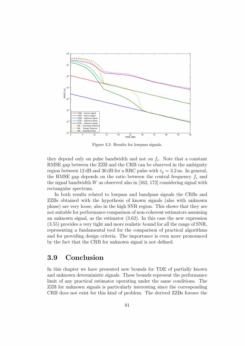
0 5 10 15 20 25 30 35 40 45 5010
−5
10−4
10−3
10−2
10−1
100
101
102
SNR [dB]
RM
SE
[ns]
CRB − known signalZZB − known signalCRB − unknown phaseZZB − unknown phaseZZB − unknown signalML − Envelope DetectorML − Energy DetectorML − Matched Filter
Figure 3.2: Results for lowpass signals.
they depend only on pulse bandwidth and not on fc. Note that a constantRMSE gap between the ZZB and the CRB can be observed in the ambiguityregion between 12 dB and 30 dB for a RRC pulse with τp = 3.2 ns. In general,the RMSE gap depends on the ratio between the central frequency fc andthe signal bandwidth W as observed also in [162, 172] considering signal withrectangular spectrum.
In both results related to lowpass and bandpass signals the CRBs andZZBs obtained with the hypothesis of known signals (also with unknownphase) are very loose, also in the high SNR region. This shows that they arenot suitable for performance comparison of non-coherent estimators assumingan unknown signal, as the estimator (3.62). In this case the new expression(3.55) provides a very tight and more realistic bound for all the range of SNR,representing a fundamental tool for the comparison of practical algorithmsand for providing design criteria. The importance is even more pronouncedby the fact that the CRB for unknown signal is not defined.
3.9 Conclusion
In this chapter we have presented new bounds for TDE of partially knownand unknown deterministic signals. These bounds represent the performancelimit of any practical estimator operating under the same conditions. TheZZB for unknown signals is particularly interesting since the correspondingCRB does not exist for this kind of problem. The derived ZZBs foresee the
81

presence of different regions, clearly showing the SNRs threshold values of theambiguity region, where the signal observation adds a little contribution tothe estimation performance, and of the asymptotic region, where the estima-tor performance is correctly predicted by the CRB (when exists). Moreoverthe proposed new bound for unknown signals results very tight consideringthe real performance of ML estimators based on energy measurements on thereceived signal, as it is the usual approach for the case of unknown signalshape.
3.A Series Expansions of Signals
In this appendix, orthonormal series expansions are used to express the sig-nals, both random and deterministic, as a linear combination of terms, pro-viding a good approximation of the signal energy in a time-limited intervalT . When representing random processes, the classical KL expansion, lead-ing to uncorrelated coefficients, is adopted [66, 184]. These expansions allowcharacterizing the signal energy in a time-limited interval, in the presenceof Gaussian noise, with the Chi-square distribution, and their adoption isjustified by the resulting good accuracy when WT ≫ 1. In [185] it has beenshown that the accuracy is quite good also for moderate and small WT . Inthis chapter we adopt the conventional expansion also for small WT , extend-ing the derivation to the case 2WT < 1 for lowpass signals and WT < 1 forbandpass signals.
3.A.1 Series Expansion of Baseband Random Signals
Consider a zero mean, wide-sense stationary (WSS), Gaussian random pro-cess n(t) with a flat power spectral density N0/2 in [−W,W ] observed int ∈ [0, T ]. Its autocorrelation function is Rn(τ) = N0W sinc (2Wτ), with
sinc (x) , sin(πx)πx
for x 6= 0 and sinc (0) , 1.The classical KL series expansion of n(t) over the interval [0, T ] is21
n(t) =
∞∑
m=1
√λm cmΦm(t) (3.64)
where {cm} are independent zero mean Gaussian r.v.s with unitary variance,whereas Φm(t) and λm are, respectively, the eigenfunctions and eigenvalues
21The equality in (3.64) means mean square convergence, i.e.,
limM→∞
E
{∣∣∣n(t)−∑M
m=1
√λm cm Φm(t)
∣∣∣2}
= 0.
82

of the integral equation [66, p. 180]∫ T
0
Rn(t− τ) Φm(τ) dτ = λmΦm(t) . (3.65)
The eigenfunctions of (3.65), which form a set of complete orthonormal func-tions {Φm(t)} with support [0, T ],22 are prolate spheroidal wave functions[186, 187], whereas the corresponding eigenvalues are given by
λm = N0W T[R
(1)0m(πW T, 1)
]2(3.66)
being R(1)0m(x, 1) the radial prolate spheroidal function [186]. The coefficient
λm c2m corresponds to the energy along the coordinate function Φm(t) of aparticular random process sample. Therefore the energy of a sample of n(t)is
En =
∫ T
0
n2(t) dt =
∞∑
m=1
λm c2m . (3.67)
It has been shown in [186, 188, 189] that for 2WT ≫ 1 the eigenvaluesλm rapidly drops to zero for m > ⌊2WT ⌋ + 1, leading to the well-known“2WT-theorem” [190, 191],[192, p.128], according to which the series can betruncated to the first N = ⌊2WT ⌋ + 1 terms. Moreover it is λm ≈ N0
2for
1 ≤ m ≤ 2WT , and zero otherwise, so that
n(t) ≈√
N0
2
N∑
m=1
cmΦm(t) (3.68)
and [86]23
En =
∫ T
0
n2(t) dt ≈ N0
2
N∑
m=1
c2m . (3.69)
Approximations (3.64) and (3.69) get less accurate as 2WT approaches one,and if N ≤ 1 (i.e., T < 1/2W ), these approximations are no longer valid. Insuch a case it is possible to see [188] that λm ≈ 0 for m > 1 and [188] suggests
the approximation λ1 ≈ N0
22πc(1− c2
9
), with c = πWT . Considering the
case of very small WT , where effectively only λ1 6= 0, we adopt here theapproximation λ1 ≈ N0
πc (i.e., R
(1)01 (πW T, 1) ≈ 1), so that λ1 ≈ N0 W T , and
then
En =
∫ T
0
n2(t) dt ≈ N0W T c21 . (3.70)
22Even if not explicitly specified, functions {Φm(t)} depends on WT .23Hence we have that the expected received energy in T is given by E
{∫ T
0 n2(t) dt}=
E{∑
∞
m=1 λm c2m}= N0WT [66, p. 181].
83
3.A.2 Series Expansion of Bandpass Random Signals
Consider n(t) to be a bandpass, zero-mean, WSS, Gaussian random processwith a flat power spectral density N0/2 for |f | ∈ [−fc − W/2, fc + W/2]observed in t ∈ [0, T ]. We have that a sample function n(t) of the randomprocess can be written as n(t) = V (t) cos (2πfct+ φ(t)). Using the conven-tional approach it is [184, p.159]
n(t) = nI(t) cos(2πfc t)− nQ(t) sin(2πfc t) (3.71)
where nI(t) and nQ(t) are, respectively, the in-phase and in-quadrature base-band components of n(t). In this manner we have nI(t) = V (t) cos(φ(t)) andnQ(t) = V (t) sin(φ(t)). Moreover, the random processes related to nI(t) andnQ(t) are statistically independent, zero-mean Gaussian processes.24 It canbe shown that their spectral densities are confined to the region |f | < W/2with intensity N0. The baseband components can be expanded in orthonor-mal series as previously discussed
nI(t) ≈√
N0
N/2∑
m=1
c1,mΦm(t) ,
nQ(t) ≈√
N0
N/2∑
m=1
c2,mΦm(t) (3.72)
with c1,m and c2,m independent zero mean Gaussian r.v.s with unitary vari-ance, and N = 2(⌊WT ⌋+ 1). Therefore
En =
∫ T
0
n2(t) dt ≈ 1
2
∫ T
0
n2I(t) dt+
1
2
∫ T
0
n2Q(t) dt =
N0
2
N∑
m=1
c2m (3.73)
having defined c2m−1 = c1,m and c2m = c2,m for m = 1, 2, . . . , N/2. Note thatthis expression is identical to (3.69). This means that all the analysis carriedout for baseband signals still applies for bandpass signals when WT ≫ 1.
When ifN ≤ 2 (i.e., T < 1/W ), the hypothesis of large T appears difficult
24This requires that spectral density is narrow with respect to the central frequency,i.e., the envelope V (t) and the phase φ(t) are slowly varying functions of the time, andthe observation time T is large enough [184, p. 158].
84

to validate. In fact, this corresponds to the assumption that
En =
∫ T
0
n2(t) dt =
∫ T
0
n2I(t) cos
2(2πfct) dt+
∫ T
0
n2Q(t) sin
2(2πfct) dt
− 2
∫ T
0
nI(t)nQ(t) cos(2πfct) sin(2πfct) dt
≈ 1
2
∫ T
0
n2I(t) dt+
1
2
∫ T
0
n2Q(t) dt . (3.74)
If (3.74) is verified with satisfactory approximation,25 we have that the ap-proach followed for lowpass signals in Appendix 3.A.1 still applies. In thiscase we obtain
EnI=
∫ T
0
n2I(t) dt ≈ N0W T c21,1 ,
EnQ=
∫ T
0
n2Q(t) dt ≈ N0W T c22,1 (3.75)
and
En =
∫ T
0
n2(t) dt ≈ N0W T
2
(c21,1 + c22,1
)=
N0W T
2
(c21 + c22
). (3.76)
3.A.3 Series Expansion of Baseband Deterministic Sig-
nals
In the case of a deterministic signal s(t) observed in the interval [0, T ],there is a complete degree of freedom in choosing the orthonormal basis.Often the sampling expansion, considering the orthonormal base Ψn(t) =√2W sinc (2Wt− n),26 is adopted [190, 191]
s(t) ≃ 1√2W
N∑
n=1
sn Ψn(t) (3.77)
where sn = s(n/2W ) are the samples of s(t) taken at Nyquist rate 2W overthe interval [0, T ]. Also in this case, for 2WT ≫ 1 the following approxima-
25We will show in the numerical result that, for our problem, approximation (3.74) issatisfactory also for wideband signals.
26Note that, differently from {Φm(t)}, the base {Ψn(t)} is not concentrated in theinterval [0, T ].
85

tion for the energy of s(t) in the interval [0, T ] holds [190, 176, 86]27
∫ T
0
s2(t) dt ≈ 1
2W
N∑
n=1
s2n . (3.78)
In the detector derivation presented in Sec. 3.6.2, it results necessary torepresent the signal in a portion [0, z] of the interval [0, T ], with z < T .In order to obtain a satisfactory approximation also when z < 1/2W , it isimportant to adopt the basis {Φm(t)}, where now {Φm(t)} is related to theinterval W z, obtaining
s(t) ≈M∑
m=1
ηmΦm(t) . (3.79)
3.A.4 Series Expansion of Bandpass Deterministic Sig-nals
Consider the signal s(t) as deterministic and bandpass, with non-zero Fouriertransform in |f | ∈ [−fc − W/2, fc + W/2], observed in t ∈ [0, T ]. We canrepresent it by its ELP s(t), that is s(t) = ℜ
{s(t) e2πfct
}. The ELP can be
decomposed as s(t) = sI(t) + sQ(t), therefore we obtain
s(t) = sI(t) cos(2πfct)− sQ(t) sin(2πfct) , (3.80)
where the in-phase and in-quadrature baseband components sI(t) and sQ(t)have a spectrum confined to |f | ≤ W/2. We can then apply all the deriva-tion presented in Appendix 3.A.3 to each of the two baseband components,adopting the expansions
sI(t) ≈M∑
m=1
η1,mΦm(t) (3.81)
sQ(t) ≈M∑
m=1
η2,mΦm(t) (3.82)
with η1,m and η2,m the series expansion coefficients of sI(t) and sQ(t) fort ∈ [0, T ].
27However, the representation error obtained when adopting {Ψn(t)} is higher than with{Φn(t)} that lead to the best approximation in t ∈ [0, T ] [176].
86

3.B Proof of Equation (3.11)
Recalling (3.10) we have that r = H(τ) s + n = y + n. Consider a dif-ferent orthonormal bases for r(t) according to which the series expansioncoefficients are written as r = S(τ) s + n = y + n. In order to prove
that H(τ)(H(τ)TH(τ)
)−1
H(τ)T r corresponds to the expansion of the signal
r(t) Π(
t−τTs
)for t ∈ [0, Tob], we can try to recover the same results from the
expansion S(τ)(S(τ)TS(τ)
)−1
S(τ)T r. It is now convenient to choose S(τ) so
that r represents the samples of the received signal in [0, Tob], and s repre-sents the samples of the transmitted signal in [0, Ts]. In this case it is easyto show that S(τ) has the block structure
S(τ) = [0T,N , IN , 0M−N−T,N ]T (3.83)
with T = ⌈τ/2W ⌉,28 0A,B the A × B null matrix and IN the Nth orderidentity matrix. Moreover, matrix S(τ) contains N linearly independent vec-
tors (it forms an orthonormal basis), and PS(τ) = S(τ)(S(τ)TS(τ)
)−1
S(τ)T =
S(τ)S(τ)T . It is immediate to show that
PS(τ) =
0T,T 0T,N 0T,M−N−T
0N,T IN 0N,M−N−T
0M−N−T,T 0M−N−T,N 0M−N−T,M−N−T
(3.84)
and PS(τ)r = [0T , r[T + 1], r[T + 2], r[T +N ], 0M−N−T ]T , from which results
the quadratic form rTPS(τ)r =∫ τ+Ts
τr2(t) dt, that is (3.11) where r(t) is a
generic x(t).29
3.C Asymptotic Expression of Pmin (z)
Adopting, as approximation, the lower bound derived in [193] for the MarcumQ-function30
Q1(α, β) ≥ e−α2+β2
2 I0(αβ) (3.85)
we obtain
Pmin (z) ≃1
2e−
SNR
2 I0
(SNR
2|ρ0(z)|
)(3.86)
28We consider, for convenience, the lowpass signal case.29Note that PS(τ) is positive definite.30This bound, valid for β > α is very tight especially for high β (i.e., high SNR), see
also [194].
87

since a2(z) + b2(z) = SNR and a(z)b(z) = SNR
2|ρ0(z)|. Considering that
I0(x) ≃ ex√2πx
for large x [106, p. 377] we obtain
Pmin (z) ≃1√
4πSNR|ρ0(z)|exp
{−SNR
2(1− |ρ0(z)|)
}. (3.87)
Adopting now the approximation for the Gaussian Q-function[195]
Q(x) ≃ 1√2πx2
e−x2
2 (3.88)
we obtain (3.31).
3.D Derivation of P {Y1 < Y2}In this appendix we derive P {Y1 < Y2}. Y1 and Y2 are defined in 3.6 with, re-spectively, non-central Chi-square p.d.f. fNC(y, µ, ν), and central Chi-squarep.d.f. fC(y, ν), where µ = 2γ is the non-centrality parameter and ν = 2q arethe degrees of freedom, that is
fNC(y, µ, ν) =1
2e−
y+µ2
(y
µ
)ν−24
I ν2−1(
√yµ) , y ≥ 0,
fC(y, ν) =y(
ν2−1)
2ν2Γ(ν2
) e− y2 , y≥0 (3.89)
with Iκ(·) the κth order modified Bessel function of the first kind [106, p.374] and Γ(·) the Gamma function [106, p. 255].
Consider two new r.v.s R1 and R2 where R1 =√Y1 and
√Y2. The p.d.f.s
of R1 and R2 can be found using the r.v.s transformation rule as follows
fR1(r1) = 2 r1fNC(r21, µ, ν) ,
fR2(r2) = 2 r2fC(r22, ν) . (3.90)
From (3.90), the cumulative distribution function (c.d.f.) of R2 can be ob-tained as
FR2(r2) =
∫ r2
0
2tt2(q−1)
2q Γ(q)e−
t2
2 dt . (3.91)
Adopting the transformation t2
2= ξ we obtain
FR2(r2) =1
Γ(q)
∫ r222
0
ξ(q−1)e−ξ dξ =1
Γ(q)γ
(q,
r222
)(3.92)
88
where γ(·, ·) is the lower incomplete gamma function [106, p. 260].
Since γ(n, x) = Γ(n)(1− e−x
∑n−1i=0
xi
i!
)we get
FR2(r2) = 1− e−r222
q−1∑
i=0
1
i!
(r222
)i
. (3.93)
By using (3.90) and (3.93), we can rewrite P {Y1 < Y2} as
P {Y1 < Y2} = P {R1 < R2} = 1− P {R2 < R1}
= 1−∫ ∞
0
FR2(r1)fR1(r1) dr1
= 1−∫ ∞
0
[1− e−
r212
q−1∑
i=0
1
i!
(r212
)i]fR1(r1) dr1
=
∫ ∞
0
rq1 e− r21+µ
2 µ− q−12 Iq−1 (r1
√µ) e−
r212
q−1∑
i=0
1
i!
(r212
)i
dr1
= e−µ2 µ− q−1
2
q−1∑
i=0
1
i! 2i
∫ ∞
0
rq+2ie−r2Iq−1 (r√µ) dr. (3.94)
The following integral is given in [196]31
∫ ∞
0
xm−1 exp(−a2x2
)In (bx) dx =
bnΓ(m+n2
)
2(n+1)a(m+n)Γ(n+ 1)exp
(b2
4a2
)
×1F1
(n−m
2+ 1;n+ 1;− b2
4a2
)
(3.95)
where 1F1(·; ·; ·) is the confluent hypergeometric function of the first kind32
[106, ch. 13] that is
1F1 (c1; c2; x) ,∞∑
k=0
(c1)k(c2)k
xk
k!(3.96)
where (d)k , Γ(d + k)/Γ(d) is the Pochhammer symbol [106, p. 256]. Bysubstituting (3.95) in (3.94), we obtain
P {Y1 < Y2} =e−
µ4
2q Γ(q)
q−1∑
i=0
Γ(q + i)
i! 2i1F1
(−i; q;−µ
4
). (3.97)
31The expression is derived from [197, p. 394]. An equivalent expression in given in[106, p. 486].
32Also referred as Kummer’s function [106, p. 504].
89

The function 1F1 (−c1; c2; x) for c1 > 0 and c2 > 0, as in this case, can berewritten as a finite summation [106, p. 509], that is
1F1 (c1; c2; x) =c1!
(c2)c1L(c2−1)c1
(x) (3.98)
having indicated with Lαn(x) the associated Laguerre polynomial given by33
Lαn(x) ,
n∑
m=0
(−1)m(n+ α)!
(n−m)!(α +m)!m!xm . (3.99)
This leads to the following expression
P {Y1 < Y2} =e−
µ4
2q
q−1∑
i=0
1
2i
i∑
j=0
(i+ q − 1)!
(i− j)!(j + q − 1)!j!
(µ4
)j. (3.100)
We can now rearrange (3.100) obtaining the final formulation
P {Y1 < Y2} =e−
µ4
2q
q−1∑
i=0
(µ4
)i
i!
q−1∑
k=i
(k + q − 1)!
2k(k − i)!(k + q − 1)!. (3.101)
33Also referred as generalized Laguerre polynomial [106, p. 775].
90

Part III
Location-Awareness
91

Introduction
High-accuracy network localization is essential for a variety of wireless ap-plications including logistic, search and rescue, automotive, medical services,security tracking and military systems, and results one of the key enablingfeatures of context-aware networks [52]. Network localization is usually real-ized by an infrastructure including tagged nodes (agents or tags) attached toor embedded in objects and of reference nodes (anchors) placed in known po-sitions, which communicate with tags through wireless signals to determinetags’ location [198, 199, 24].
Common methods to determine the position of tags are based on fea-tures measurement from received waveforms, such as TOA, time difference-of-arrival (TDOA), RSSI, and angle-of-arrival (AOA). The choice of thefeatures affects significantly the localization accuracy [24].
Future real time locating systems (RTLS) are expected to provide reliableand secure high-accuracy localization of objects while maintaining low powerconsumption and costs. This is challenging especially in harsh propagationenvironments such as indoor and urban canyon. In this perspective, UWBtechnology offers the potential of achieving high ranging accuracy throughsignal TOA measurements due to its ability to resolve multipath [47, 51].Other advantages of UWB include, low power consumption at the transmitterside, robustness to multipath, low detection probability, and large numbersof devices that can coexist in the same area. These properties encouragedthe adoption of UWB radio for active tags (i.e., devices equipped with aradio transmitter), in localization systems [134, 200, 201]. Passive tags basedon backscattered signaling have been recently proposed for next generationRFID and low-cost localization systems [50] and will be analyzed in the lastpart of this thesis.
The presence of obstacles in real propagation environments generatesNLOS channel conditions that may severely degrade ranging accuracy due todirect path blockage, direct path excess delay, lowering of the SNR [202, 28].NLOS conditions can also disable ranging, leading to a limitation of the areacovered by the localization system. Several NLOS mitigation approacheshave been presented in the literature to improve the localization accuracyin NLOS conditions [203, 204, 205]. All these methods and similar assumethat, even in NLOS, a signal exchange between nodes is possible with certainamount of degradation. Unfortunately in many scenarios the signal might becompletely obstructed by obstacles thus making the above-mentioned tech-niques not effective.
In the presence of severe NLOS conditions, a typical solution consistsin increasing the number of anchors at the expense of higher infrastructure
93

and deployment costs.34 Despite the possibility of increasing the number ofanchors, several different approaches can be adopted for improved networklocalization in these situations. First of all, the possibility of cooperationamong tags can be considered [137, 52, 28, 206].
Chapter 4 presents the results of several experimentation campaign ori-ented to investigate the advantages of cooperation between nodes, of theprior knowledge of the environment and of the identification of the channelstate (i.e., LOS/NLOS) in the positioning process.
Unfortunately cooperation can be exploited only by active tags equippedwith sufficient computational capability, often in contrast with low cost re-quirements. In addition, it has to be remarked that area coverage for lo-calization systems is more demanding than area coverage in communicationsystems because at least three anchors must be visible simultaneously by atag in each position to make tag localization in two-dimension feasible with-out ambiguity. On the other hand, many applications pose several constraintson infrastructure cost, thus a reduction of the number of anchors is desirableregardless the presence of NLOS conditions. To address this issue and enablelocalization with satisfactory performance also in non-cooperative networks,Chapter 5 introduces the idea of relaying techniques for localization, provid-ing practical solutions and performance analysis.
34Note also that anchors have to be tightly time synchronized if time-based positioningapproaches are adopted.
94

Chapter 4
Experimentation forCooperative Localization
4.1 Motivations
Cooperation among peer nodes at the physical layer can significantly expandthe capabilities of wireless networks [207, 208, 209, 210]. In context-awarenetworks cooperation between nodes can be successfully exploited to improvethe performance and to reduce the outages due to an insufficient number ofanchors in visibility of a certain node [137, 211]. The performance of suchnetworks depends on the conditions of each link, and thus the experimentalcharacterization of channels associated with all links is essential for the designof cooperative wireless networks.
For what concerns the characterization of cooperative location-aware net-works, the following two kinds of measurements are necessary for all links:1
• range measurements for estimating the link distance between each pairof nodes; and
• waveform measurements for estimating the range and channel stateassociated with each link,
both of which are used as inputs to the localization algorithms. Network ex-perimentation based on waveform measurements enables the characterizationof cooperative wireless networks for various applications. While there havebeen numerous works on measurements and models of wireless environments
1In principle range information can be extracted from received waveforms. However,this could require network synchronization. In our experimental setting, this is alleviatedby radios that enable the collection of range and waveform measurements simultaneously.
95

[212, 213, 214, 215, 216, 217, 218, 56, 55, 114, 219, 105, 57], they have mainlyfocused on point-to-point channels.
Providing location-awareness in cluttered environments is challenging pri-marily due to multipath, LOS blockage, and excess propagation delays throughmaterials.2 UWB technology [47, 48, 220] can provide accurate localization[136, 134, 24] in such environments [200, 138, 221, 222, 134] due to its abilityto resolve multipath and penetrate obstacles [54, 53, 218, 56, 55, 114]. UWBsignals provide fine delay resolution, enabling precise TOA measurementsfor range estimation between two nodes [135, 223, 224, 51]. However, theaccuracy and reliability of range-based localization techniques typically de-grade in cluttered environments, where multipath, LOS blockage, and excesspropagation delays through materials lead to positively-biased range mea-surements [51, 225].
We consider in this chapter the problem of network localization in realis-tic indoor environments, involving anchors (also referred to as beacons) andagents (also referred to as tags or targets). In a noncooperative setting, eachagent estimates the distances from neighboring anchors, which are then usedas inputs to a localization algorithm for determining its own position. Ina cooperative setting, each agent estimates the distances from neighboringagents in addition to that from neighboring anchors. The localization processconsists of a measurement phase where agents perform measurements withanchors and others agents (in a cooperative setting), and a location updatephase where agents infer their position based on prior knowledge and newmeasurements. The performance of localization algorithms depends mainlyon two factors: (i) the geometric configuration of the network described bythe positions of anchors and agents, and (ii) the quality of measurementsaffected by the propagation conditions of the environment [134, 51, 137].Localization performance can be improved significantly by selecting appro-priate anchors [138, 137, 226] and mitigating the effects of unreliable rangemeasurements [227, 204].
In this chapter, results of several measurement campaigns are presented,providing a methodology particularly suited for cooperative wireless net-works. This enables the performance evaluation of various network local-ization algorithms under a common setting. The key contributions of thechapter can be summarized as follows:
• Development of experimentation methodology for the characterizationof cooperative wireless networks in realistic environments;
2In these environments (e.g., inside buildings, in urban canyons, under tree canopies,and in caves), the global positioning system (GPS) is often inaccessible.
96

(a) Environment A: Wireless Communi-cations Laboratory at Univ. of Bologna.
(b) Environment B: Engineering Facultyat Univ. of Bologna (Cesena campus).
Figure 4.1: The experimentation environments.
• Establishment of database with range and waveform measurements forcooperative wireless channels; and
• Presentation of experimental results related to localization in LOS andNLOS conditions.
The remainder of the chapter is organized as follows. The experimen-tation methodology for cooperative location-aware networks is presented inSec. 4.2. In Sec. 4.3, a range error model is introduced. Section 4.4 describestechniques for range error mitigation and position refinement. Finally, a con-clusion is given in Sec. 4.5.
4.2 Network Experimentation Methodology
We now describe the network experiments for design and analysis of coop-erative location-aware networks under a common set of measurements. Theperformance of such networks is dominated by the behavior of range errors.Range estimates based on TOA measurements are typically corrupted bythermal noise, multipath fading, direct path (DP) blockage, and DP excessdelay [51]. A range measurement is referred to as a DP measurement if it isobtained from a signal traveling along a straight line between the two nodes.A measurement is non-DP if the DP signal is completely obstructed (i.e., DP
97

1 2 3 4 5 6 7 8 9 10 11 12 13 14 15 16 17 18 19 20
1
2
3
4
5
6
7
8
9
10
11
12
13
14
15
16
17
18
19
20
Figure 4.2: Connectivity matrix for the environment B.
blockage) and the first signal to arrive at the receiver comes from reflectedpaths only. Another source of error is the DP excess delay caused by thepropagation of a partially obstructed DP components that travels throughdifferent obstacles (e.g., walls in buildings).3
An important observation to be made is that DP blockage and DP excessdelay have the same effects on range measurements: they both add a positivebias to the true distance between the nodes. These measurements are referredto as NLOS measurements. A LOS measurement occurs when the signaltravels along an unobstructed DP.
The geometry of the network, the measurements of all links, and measure-ments through obstacles, all of which affect the performance of cooperativewireless networks, are described in the following.
4.2.1 Network Geometry
We consider wireless networks in realistic indoor environments with a geo-metric configuration consisting of Nb anchors deployed in known positions todetermine the unknown positions of Na agents. In particular, we chose a set
3Given a homogeneous material with relative electrical permittivity ǫr, the speed ofthe electromagnetic wave traveling inside materials is slowed down by a factor
√ǫr with
respect to the speed of light c. Hence the extra delay introduced by a wall of thickness dWis ∆ ≃
(√ǫr − 1
)dW/c (considering wideband signals, since ǫr is frequency-dependent, a
signal distorsion is also present).
98

(a) A view of measurement setup. (b) Through a wall measurement.
Figure 4.3: A typical apartment in Bologna, Italy, serving as the network experimentationenvironment.
of positions for anchors and agents, and performed simultaneous range andwaveform measurements for all possible links between pairs of nodes.4 Twomeasurement campaigns have been carried out: (i) in a typical apartmentwith furniture and concrete walls with thickness of 15 and 30 cm (envi-ronment A); and (ii) in a typical office indoor environment with furnitureand drywall with thickness of 10 cm (environment B). In the environment A,Np = 25 possible node positions of which Nb = 5 are anchors (labeled B1-B5)and Na = 20 are agents (numbered 1-20) are considered. In the environmentB, Np = 20 possible nodes positions (numbered 1-20) are considered, despitethe adoption as anchors or agents.
As example, considering environment A, range and waveform measure-ments for each pair of anchor and agent were made for a noncooperativesetting (i.e., 5× 20 possible links). In addition, measurements between eachpair of agents were also made for a cooperative setting (i.e., additional
(202
)
possible links). A total of 1500 measurements were collected for each pair ofnodes in both environments, whose maps are reported in Fig. 4.1.
Note that NLOS situations can significantly reduce the SNR at receiverside so that, in some situations, a link between two nodes cannotexist, dueto the impossibility of detecting the presence of the signal by the receivingradio. In this case the number of connections is obviously less than in a fullyconnected network. Figure 4.2 shows this fact presenting, as example, theconnectivity matrix related to measurements performed in environment B.
4In general, the selection of nodes positions can be based on a grid or by choosing keypositions in the environment (e.g., particular places in a room or in a corridor).
99
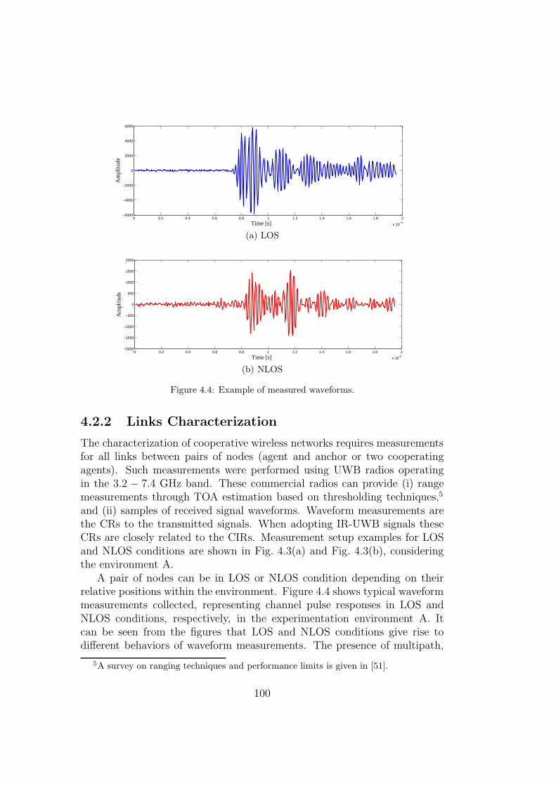
0 0.2 0.4 0.6 0.8 1 1.2 1.4 1.6 1.8 2
x 10−8
−6000
−4000
−2000
0
2000
4000
6000
Time [s]
Am
plitu
de
(a) LOS
0 0.2 0.4 0.6 0.8 1 1.2 1.4 1.6 1.8 2
x 10−8
−2000
−1500
−1000
−500
0
500
1000
1500
2000
Time [s]
Am
plitu
de
(b) NLOS
Figure 4.4: Example of measured waveforms.
4.2.2 Links Characterization
The characterization of cooperative wireless networks requires measurementsfor all links between pairs of nodes (agent and anchor or two cooperatingagents). Such measurements were performed using UWB radios operatingin the 3.2 − 7.4 GHz band. These commercial radios can provide (i) rangemeasurements through TOA estimation based on thresholding techniques,5
and (ii) samples of received signal waveforms. Waveform measurements arethe CRs to the transmitted signals. When adopting IR-UWB signals theseCRs are closely related to the CIRs. Measurement setup examples for LOSand NLOS conditions are shown in Fig. 4.3(a) and Fig. 4.3(b), consideringthe environment A.
A pair of nodes can be in LOS or NLOS condition depending on theirrelative positions within the environment. Figure 4.4 shows typical waveformmeasurements collected, representing channel pulse responses in LOS andNLOS conditions, respectively, in the experimentation environment A. Itcan be seen from the figures that LOS and NLOS conditions give rise todifferent behaviors of waveform measurements. The presence of multipath,
5A survey on ranging techniques and performance limits is given in [51].
100

b)
������������
���������
���������
���������
���������
���������
���������
����
����
����
����������������������������������
����������������������������������
ranging device ranging device
ranging device ranging device
15cm 30cm
a)
dW��������������������������������������������������
��������������������������������������������������
���������������������������
���������������������������
������������������������������������
������������������������������������������
Figure 4.5: Obstacles characterization setup [228].
typical of indoor environments, is also noticeable in both waveforms. Theknowledge of the NLOS condition can be exploited to mitigate ranging errorsto significantly improve the performance of the localization algorithms.
Let di,j denotes the Euclidean distance between two nodes (i.e., an agentand a reference node, which can be either an anchor or a cooperative agent) inpositions pi and pj , respectively. Note that UWB radios provide ranging ac-curacy on the order of a few centimeters, and thus the true distance betweeneach pair of nodes must be measured with an accuracy better than a cen-timeter. On the other hand, measuring the true distance between two nodeswith obstacles (e.g., walls) in between can be difficult even using laser-basedranging devices. This difficulty is alleviated by using a 3D computer-aideddesign software.
4.2.3 Obstacles Characterization
To characterize the bias of ranging errors due to obstacles, additional rangemeasurements were collected in the environment. The transmitting and re-ceiving nodes were placed in several positions, such that one or two wallswith different thicknesses were present between the two nodes, according to
101

Layout, dW [cm] mean bias [cm] std dev [cm]1 wall, 15.5 16.4 3.71 wall, 30 29.5 3.22 walls, 15.5+30 45.2 3
Table 4.1: Mean and standard deviation of ranging bias for different wall thicknesses.
Fig. 4.5. Range measurements were collected using UWB radios located infive sets of short distances (i.e., 20, 40, 60, 80, and 100 cm from both sidesof the walls) to isolate the effects of excess delay from those of multipath. Aview of the measurement setup is given in Fig. 4.3(b). By using the collectedrange measurements ensemble (5 × 1500 measurements in total), the mean(bias) and standard deviation of range errors were calculated respectively as:16.4 cm and 3.7 cm for one wall with thickness dW = 15.5 cm; 29.5 cm and3.2 cm for one wall with dW = 30.0 cm; and 45.2 cm and 3.0 cm for two wallswith total dW = 15.5 + 30.0 cm (see also Tab. 4.1).
As can be noted, the bias appears to increase with the thickness of thewall. The low value of the standard deviation indicates that the range errorsare dominated by the effects of excess delay rather than those of multipathand thermal noise. From the collected ensemble of measurements we observethat ∆ ≃ dW/c, thus ǫr ≃ 4.6
In the following sections, the measurements from our network experimentswill be used to model ranging errors as well as to analyze signal processingtechniques able to improve the localization performance.
4.3 Range Error Model
Understanding the behavior of range errors is essential for the developmentof cooperative localization techniques. In the following, range model basedon measurements in Sec. 4.2.2 and range error bias model based on measure-ments in Sec. 4.2.3 will be developed.
We start by categorizing these link measurements in Section 4.2.2 in termsof the channel state (e.g., the state Hi indicates i walls between a pair ofnodes with i = 0, 1, ..., 4). Figure 4.6 shows the range error bias (i.e., averagerange error over 1500 measurements) for each link as a function of the truedistance, in LOS (H0) and NLOS (H1, H2, H3, and H4) conditions. Notethat the bias depends strongly on the total thickness of the walls. Range
6The value of ǫr, which depends on the material of the wall, is confirmed by a similarresult obtained in [229]. See also [230] for a more accurate wall behavior characterization.
102
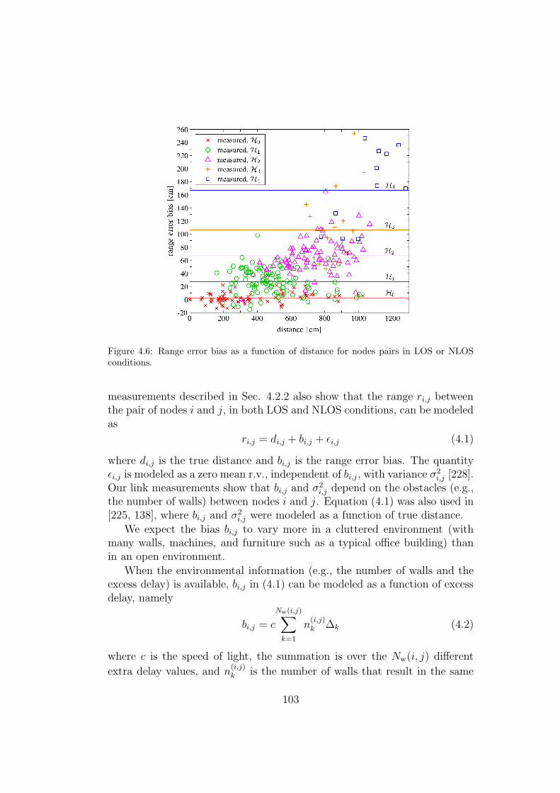
Figure 4.6: Range error bias as a function of distance for nodes pairs in LOS or NLOSconditions.
measurements described in Sec. 4.2.2 also show that the range ri,j betweenthe pair of nodes i and j, in both LOS and NLOS conditions, can be modeledas
ri,j = di,j + bi,j + ǫi,j (4.1)
where di,j is the true distance and bi,j is the range error bias. The quantityǫi,j is modeled as a zero mean r.v., independent of bi,j , with variance σ2
i,j [228].Our link measurements show that bi,j and σ2
i,j depend on the obstacles (e.g.,the number of walls) between nodes i and j. Equation (4.1) was also used in[225, 138], where bi,j and σ2
i,j were modeled as a function of true distance.
We expect the bias bi,j to vary more in a cluttered environment (withmany walls, machines, and furniture such as a typical office building) thanin an open environment.
When the environmental information (e.g., the number of walls and theexcess delay) is available, bi,j in (4.1) can be modeled as a function of excessdelay, namely
bi,j = c
Nw(i,j)∑
k=1
n(i,j)k ∆k (4.2)
where c is the speed of light, the summation is over the Nw(i, j) different
extra delay values, and n(i,j)k is the number of walls that result in the same
103
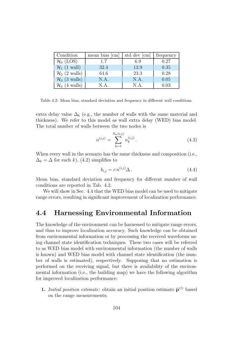
Condition mean bias [cm] std dev [cm] frequencyH0 (LOS) 1.7 6.9 0.27H1 (1 wall) 32.4 13.9 0.35H2 (2 walls) 64.6 23.3 0.28H3 (3 walls) N.A. N.A. 0.05H4 (4 walls) N.A. N.A. 0.03
Table 4.2: Mean bias, standard deviation and frequency in different wall conditions.
extra delay value ∆k (e.g., the number of walls with the same material andthickness). We refer to this model as wall extra delay (WED) bias model.The total number of walls between the two nodes is
n(i,j) =
Nw(i,j)∑
k=1
n(i,j)k . (4.3)
When every wall in the scenario has the same thickness and composition (i.e.,∆k = ∆ for each k), (4.2) simplifies to
bi,j = c n(i,j)∆ . (4.4)
Mean bias, standard deviation and frequency for different number of wallconditions are reported in Tab. 4.2.
We will show in Sec. 4.4 that the WED bias model can be used to mitigaterange errors, resulting in significant improvement of localization performance.
4.4 Harnessing Environmental Information
The knowledge of the environment can be harnessed to mitigate range errors,and thus to improve localization accuracy. Such knowledge can be obtainedfrom environmental information or by processing the received waveforms us-ing channel state identification techniques. These two cases will be referredto as WED bias model with environmental information (the number of wallsis known) and WED bias model with channel state identification (the num-ber of walls is estimated), respectively. Supposing that no estimation isperformed on the receiving signal, but there is availability of the environ-mental information (i.e., the building map) we have the following algorithmfor improved localization performance:
1. Initial position estimate: obtain an initial position estimate p(1) basedon the range measurements;
104
2. Range error mitigation: mitigate bias of the range error from measure-ments according to the bias model and the initial position estimatep(1);
3. Position refinement: update the position estimate p(2) with the cor-rected range values.
Specifically the step (2) consists in subtract, from the ranging estimates, thebias provided by the number of walls which the signal is supposed to hascrossed given the position estimate p(1).7
Differently, if prior knowledge of the environment map is not available,but it is possible to estimate the number of walls from the receiving signalwe have the algorithm:
1. Range error correction: mitigate bias of the range error from measure-ments according to the bias model and the estimated channel condi-tions;
2. Position refinement: obtain the position estimate p with the correctedrange values.
It is clear how, in this case, the first position estimation is avoided. How-ever, although the reduced complexity in the positioning algorithm, there isan increase in the signal processing part due to the waveform elaborationnecessary for extracting environmental conditions information (i.e., estima-tion of the number of walls). Note that, in this case, range measurementsare processed according to the estimation results performed on the receivedwaveforms. In the following section an example of this estimation process,with numerical results obtained exploiting the described measurements cam-paigns, is provided.
4.4.1 Previous Works
Several techniques have been proposed recently in order to identify channelconditions in terms of obstruction [203, 231, 232, 233, 234, 235, 236, 237, 238,239, 240, 241, 242, 204, 243]. Obstruction detection is generally performedby extracting a certain feature from the received waveform that varies withdifferent channel conditions. For example in [238] the identification is basedon the first peak amplitude of the received signal and delay between the first
7Obviously, in case of a high estimation error in the initial position estimate p(1) thenumber of walls can be erroneously detected with consequent error propagation.
105
and the strongest path. In [232, 233], root mean square (rms) delay-spread,mean excess delay and kurtosis parameters are used for that purpose. Thedetection can also be realized without observing the received waveform di-rectly, which is the case of the non-parametric approach proposed in [231].This work assumes that multiple and independent TOA measurements be-tween agents and anchors are available and that the change in location ofthe agents during such measurements is negligible. In these conditions, thep.d.f. of distance estimates between agent and anchor is obtained from themeasurements and is compared with the p.d.f. corresponding to LOS prop-agation. If the distance between the p.d.f.s is less than a given threshold,the channel is declared as LOS, otherwise it is stated as NLOS. Others re-cent non-parametric solutions based on machine learning can be found in[242, 204, 243]. Here some existing and new channel LOS/NLOS identifica-tion algorithms are presented and compared under common conditions.
We consider here the problem of detecting the LOS and NLOS propaga-tion conditions. However, it has been shown in [28] how it is possible, with asimilar procedure, to discriminate between the presence of one or more walls.
4.4.2 Channel State Identification Algorithms
Classic Identification Approach
Most of the LOS/NLOS identification techniques proposed in the litera-ture can be summarized according to the following classic binary detectionscheme, where the detection is performed by extracting a certain number Nof features γ = {γ1, γ2, . . . , γN} from the received signal and applying theclassical decision theory with a LRT:
p(γ|LOS)
p(γ|NLOS)
H0
≷H1
p(NLOS)
p(LOS)(4.5)
where p(γ|LOS) and p(γ|NLOS) are, respectively, the joint p.d.f.s of the setof features {γ1, γ2, . . . , γN} under LOS and NLOS conditions, p(LOS) andp(NLOS) are the prior probabilities of the LOS and NLOS events, respec-tively, H0 denotes the hypothesis of a LOS condition and H1 the presence ofa certain obstruction.
Different techniques are then often distinguished by different choice of theset γ of signal features. When more than one parameter are extracted fromthe signal, for example γ1 and γ2, obtaining the joint p.d.f. can be difficult.A sub-optimal approach is to consider γ1 and γ2 as independent random
106
variables. Then, the decision rule becomes
p(γ1, γ2|LOS)
p(γ1, γ2|NLOS)=
p(γ1|LOS)
p(γ1|NLOS)
p(γ2|LOS)
p(γ2|NLOS)
H0
≷H1
p(NLOS)
p(LOS)· (4.6)
In many practical cases, nodes that are estimating their relative distanceperform several consecutive measurements; hence, a large set of waveformsis usually available. In this case, we can decide for one or the other hypoth-esis observing the complete set of collected waveforms (assuming a quasi-stationary scenario), considering in (4.5) or (4.6) the average value of theparameter(s).
Distribution-Based Identification Approach
In this chapter we propose a different method for exploiting the complete setof waveforms instead of taking decision on the single waveform. The ideais to provide an estimation of the probability distribution of the parameterof interest, and to compare it with the reference ones corresponding to LOSand NLOS propagation. The decision is taken in favor of the hypothesis forwhich the estimated distribution is at minimum “distance” to the referenceone. The distance between distributions has to be defined according to acertain metric. Examples of such metrics are the Euclidean distance and therelative entropy or Kullback-Leibler distance. The decision criterion is thengiven by
D(pγ‖p(nlos)γ )
D(pγ‖p(los)γ )
H0
≷H1
p(NLOS)
p(LOS)(4.7)
where pγ denotes the estimated joint distribution while p(los)γ and p
(nlos)γ are
the reference distributions of the two hypotheses. For N = 1 and equal priorprobabilities for the two channel states, we have
D(pγ‖pγ(nlos))H0
≷H1
D(pγ‖p(los)γ ) . (4.8)
The experimental results related to this identification method presentedin Sec. 4.4.3 are obtained by using as metric of comparison the Euclideandistance given by
D(p‖q) =√∫ +∞
−∞[p(x)− q(x)]2dx . (4.9)
107

Features choice
A fundamental step in designing (4.5) or (4.7) is the choice of the featuresγ, extracted by observing the received signal r(t) in a certain observationinterval T , which are usually more affected by channel conditions.
The first parameter taken into account is the rms delay spread that cap-tures the temporal dispersion of the energy in a signal. It is defined as
τrms =
√∫∞0(t− τm)2|r(t)|2dt∫∞
0|r(t)|2dt (4.10)
where τm is the mean excess delay given by
τm =
∫∞0
t|r(t)|2dt∫∞0
|r(t)|2dt . (4.11)
In case of LOS propagation, the strongest path is typically the first one,while in NLOS conditions it is common to have the strongest path precededby some other smaller echoes resulting in a larger value of the delay-spread.When distributions in (4.5) are unimodal and p(LOS)=p(NLOS)1, then (4.5)is equivalent comparing γ to a suitable threshold λ corresponding to theintersection between p(γ|LOS) and p(γ|NLOS). In the delay-spread casethe decision rule takes the form
Decide :
{LOS , if τrms ≤ λτ
NLOS , if τrms > λτ
. (4.12)
Another parameter taken into account is the kurtosis, defined by
κ =1
σ4|r|T
∫
T
(|r(t)| − µ|r|
)4dt (4.13)
where µ|r| =1T
∫T|r(t)|dt and σ2
|r| =1T
∫T(|r(t)| − µ|r|)
2dt. LOS waveformsusually produce a higher value for the kurtosis. For this reason the decisionis taken as
Decide :
{NLOS , if κ < λk
LOS , if κ ≥ λk
(4.14)
where λk is the threshold value for the detection performed with this scheme.Parameters τrms and κ are strongly related to the shape of the waveform. A
1This assumption is usually considered when no a priori information is available.
108
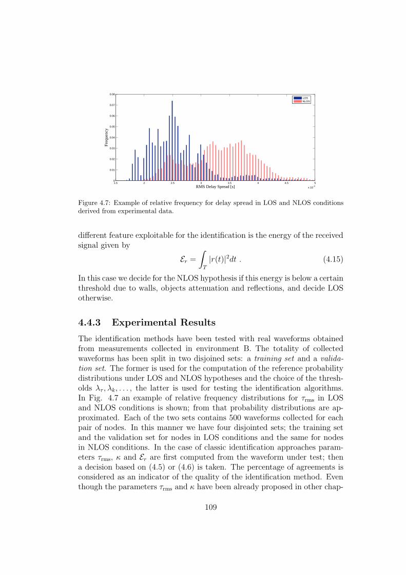
1.5 2 2.5 3 3.5 4 4.5 5
x 10−9
0
0.01
0.02
0.03
0.04
0.05
0.06
0.07
0.08
RMS Delay Spread [s]
Fre
quen
cy
LOSNLOS
Figure 4.7: Example of relative frequency for delay spread in LOS and NLOS conditionsderived from experimental data.
different feature exploitable for the identification is the energy of the receivedsignal given by
Er =∫
T
|r(t)|2dt . (4.15)
In this case we decide for the NLOS hypothesis if this energy is below a certainthreshold due to walls, objects attenuation and reflections, and decide LOSotherwise.
4.4.3 Experimental Results
The identification methods have been tested with real waveforms obtainedfrom measurements collected in environment B. The totality of collectedwaveforms has been split in two disjoined sets: a training set and a valida-tion set. The former is used for the computation of the reference probabilitydistributions under LOS and NLOS hypotheses and the choice of the thresh-olds λτ , λk, . . . , the latter is used for testing the identification algorithms.In Fig. 4.7 an example of relative frequency distributions for τrms in LOSand NLOS conditions is shown; from that probability distributions are ap-proximated. Each of the two sets contains 500 waveforms collected for eachpair of nodes. In this manner we have four disjointed sets; the training setand the validation set for nodes in LOS conditions and the same for nodesin NLOS conditions. In the case of classic identification approaches param-eters τrms, κ and Er are first computed from the waveform under test; thena decision based on (4.5) or (4.6) is taken. The percentage of agreements isconsidered as an indicator of the quality of the identification method. Eventhough the parameters τrms and κ have been already proposed in other chap-
109

Decision τrms κ Joint τrms-κ ErH0|H0 0.77 0.74 0.88 0.96H1|H1 0.79 0.77 0.79 0.87
Error Rate 0.22 0.25 0.17 0.09
Table 4.3: Classical identification approach.
Decision τrms κ Joint τrms-κH0|H0 0.81 0.96 0.93H1|H1 0.76 0.71 0.82
Error Rate 0.22 0.17 0.13
Table 4.4: Distribution-based identification approach.
ters by considering waveforms drawn from the IEEE 802.15.4a channel modelcharacterized by long channel responses (often > 100 ns) [232, 233], here thesame approach is tested on real data often characterized by shorter channelresponses (about 20 ns).
In the case of distribution-based identification approach, the observationis taken, instead of on the single waveform, on a certain number of waveformsbelonging to the validation set related to the same pair of nodes. Specificallythe decision is taken according to (4.8), having previously built the referencedistributions through the training set of waveforms, and again the percentageof agreements is taken as an indicator of the quality.
For the identification based on delay-spread and kurtosis, waveforms havebeen filtered with a band-pass filter compliant with spectral emission of thedevices used during measurements; subsequently they have been normalizedto have unitary energy. In this manner only the shape of the signal playsa role in the identification. For the identification based on received energy,waveforms have been clearly only filtered without any other type of process-ing.
Table 4.3 shows the rate of correct and incorrect channel condition iden-tification using classical detecting schemes. As can be noted, τrms and κ fea-tures give similar results. The third column considers the joint distribution(4.6) which leads to an improvement in the detection performance. Resultsrelated to the energy parameter (4.15) are reported in column 4 of Table 4.3.Surprising, the performance obtained is remarkable. Probably this result isstrictly related to the particular environment under investigation where thereis a tight correlation between low SNR and NLOS conditions.
Table 4.4 refers to the proposed distribution-based approach and showsagain the rate of correct and incorrect channel condition identification. For
110
each couple of nodes the distribution is computed using 100 waveforms ofthe validation set. We can observe how this approach gives in general betterresults especially when using the kurtosis as parameter. Even in this caseusing the joint distribution instead of considering a single parameter improvesthe detection performance.
4.5 Conclusion
The notion of network experimentation and an experimentation methodol-ogy particularly suited for cooperative wireless networks have been intro-duced. Based on this methodology extensive measurement campaigns, in-cluding ranges and waveforms measurements, have been performed. Thecollected measurements enable the modeling of range errors for both LOSand NLOS conditions and the development of channel state identificationand range error mitigation techniques. The detection of the LOS/NLOSconditions was performed with a classical binary hypothesis test using rmsdelay spread and kurtosis of the received waveforms as features for the iden-tification. The two classifiers based on these parameters provide about thesame results in terms of correct identifications. The performance can beimproved using the two parameters jointly for the test.
Further performance analysis and comparison between localization algo-rithms harnessing channel state information can be found in [28].
111

112

Chapter 5
Relaying Techniques forNetwork Localization
5.1 Motivations
When cooperation among nodes is not feasible due to the low-complexityrequirements (or the impossibility of a direct communication between pairnodes), relaying techniques can be adopted to deal with NLOS channel con-ditions.
Communication coverage can be increased by using regenerative relayscalled detect & forward (DF) [210, 244, 245, 209, 246, 247]. Localizationcoverage extension has been addressed in [248, 249, 250] for locating andtracking passive point scatterers or regenerative relays using UWB signals.An UWB localization system with a single anchor is proposed in [251] wherethe knowledge of the room geometry is exploited to map the signal reflectionsonto a set of virtual anchors. This approach requires accurate electromag-netic knowledge of the environment, which is often not available. The adop-tion of regenerative relays was proposed in [252] with the purpose to reducethe overhead and scaling inefficiencies of conventional two-way ranging ap-proaches. A similar approach based on secondary anchors performing rangingis described in [253], while in [254] regenerative relays are employed in adhoc networks composed of master and secondary active nodes for localizationwithout need for prior synchronization between the nodes.
A fundamental issue to be addressed to make relaying approaches forlocalization appealing is the complexity that must be considerably lowerthan that of the anchor nodes. The above approaches for regenerative re-lays require the same complexity of anchors because TOA estimation anddata communication capabilities are needed for the scheme to work properly.
113

Moreover, the design of regenerative relays depends on the specific signalformat adopted by the localization system. This prevents the possibility touse the same infrastructure to extend the coverage of systems adopting si-multaneously active tags, passive tags (based on backscatter modulation), orUWB WSRs for tracking moving untagged nodes.
The above-mentioned limitations can be overcome by using UWB non-regenerative relays where neither modulator nor demodulator sections arepresent in the relay and the signal is repeated as is. Non-regenerative re-lays can be active, also called amplify & forward (AF), or completely pas-sive, namely just forward (JF) (also referred to as cold repeaters). Non-regenerative relaying is well known in communication networks; for exampleJF relays are adopted as gap fillers in broadcast systems and Wi-Fi, to covershadowed areas, especially in indoor environments. Passive relay solutions in[255, 256, 257, 258] are adopted to increase the coverage of RFID systems inharsh propagation environments such as inside a metal container, pallet or aproduct container. JF relays are usually composed of a couple of intercon-nected directive antennas and take advantage of antenna directivity gain tomitigate the additional path-loss caused by obstacles [258]. Non-regenerativerelay based systems present in the literature are oriented to improve commu-nication and are not oriented to localization.
This chapter provides the basis for the design and analysis of localizationsystems with non-regenerative relaying. Both AF and JF are consideredfor coverage extension and performance improvement in harsh propagationenvironments (e.g., indoor environment with NLOS propagation conditions).ML position estimators accounting also for relayed signals are designed inorder to assess the feasibility of the approach. The benefits of the proposedsolution are quantified, enabling a direct comparison between performanceof non-relaying versus JF and AF relaying. The key contributions of thechapter can be summarized as follows:
• Introduction of the concept of non-regenerative relaying for localizationsystems;
• Analysis and design of localization systems with relays accounting fornodes deployment, propagation environment, and channel state infor-mation (CSI);
• Quantification of benefits given by relaying techniques on localizationperformance.
This chapter is organized as follows. Section 5.2 presents non-regenerativerelaying, Sec. 5.3 analyzes network localization with non-regenerative relays.
114

relay 3
furniture/obstacle
furniture/obstacle
non−regenerative tag
unit
anchor 2
non−regenerativerelay 2
to processing
furniture/obstacle
relay 1
Processing estimated position
non−regenerative
unit
anchor 1
Figure 5.1: Example of localization system employing non-regenerative relays.
Section 5.4 quantifies the impact of the proposed relaying technique for acase study, and a conclusion is given in Sec. 5.5.
5.2 System Model
We consider (see Fig. 5.1) a localization system with an infrastructure com-
posed of Na anchors located in known positions p(A)n , for n = 1, 2, . . . , Na, a
set of Nr non-regenerative unidirectional relays deployed in known positionsp(R)i , for i = 1, 2, . . . , Nr, and a generic tag in unknown position p to be
determined. Anchors are supposed to be part of a network controlled by thecentral processing unit and to have a common time scale (i.e., synchronized).
5.2.1 Non-Regenerative Relays
The purpose of relays is to repeat the signal exchange between tags andanchors. Non-regenerative relays can be passive (JF) or active (AF). Withreference to Fig. 5.2a, the JF relay is composed of a weak directional antenna(antenna A), an electrical cable and a high gain directional antenna (antennaB). The phenomenon exploited by the relay is the partial compensation ofthe additional path-loss caused by the two-hop link thanks to the directionalproperties of the antennas. Relays can be implemented in several ways.Unidirectional relays are sufficient when operating in a localization systemwith active tags adopting a one-way ranging protocol (e.g., TDOA) [24].More complex bi-directional relays are necessary in case of two-way rangingprotocols in order to ensure two-directional transmission capabilities. In thischapter we focus the attention on unidirectional relays due to their intrinsic
115

(a) JF relay
antenna A antenna B
amplifier
(b) AF relay
Figure 5.2: Non-regenerative relays.
lower complexity. In Fig. 5.2b an example of one-way AF relay is depicted.The difference with respect to the JF relay is the insertion of an amplifier inbetween antenna A and antenna B to reinforce the signal. Mutual couplingbetween antennas must be controlled through proper isolation and devicedeployment in order to avoid unstable loops caused by positive feedback thatcould arise. This effect might cause a limitation on the maximum tolerablesignal amplification level. A more complex architecture that adopts echocancelers can be also adopted in order to increase the robustness againstfeedback. Other similar solutions can be considered to this purpose (e.g.,[259]), even though they still require an external synchronization signal.
A characteristic of non-regenerative relays is the additional thermal noisegeneration. More specifically, if Ta = 290K is the antenna temperature, andG the gain of the relay (G < 1 in JF relays), the equivalent single-side noisePSD results NR = kb FR, where kb is the Boltzmann’s constant and FR is therelay noise figure (FR = 1/G in JF relays).
As general guideline, the relays are deployed in such a way that antennaB is in LOS condition with respect to one preferred anchor, and antenna Ais LOS with respect to all the possible tag positions of interest intended tobe covered by the repeater (e.g., a shadowed area).
5.2.2 Signal Model
Tags emit a signal s(t) which may be received by one or more anchors througha direct path (when LOS), through reflections from walls and obstacles, aswell as through non-regenerative relays. Tags can coexist in the same environ-ment by a suitable channelization method or a medium access control (MAC)procedure. Consider the transmitted impulse-radio UWB ranging packets(t). It is, in general, composed of a sequence of Ns UWB pulses modulated
116
according to a TH sequence {ck}, with ck ∈ {0, 1, . . .H−1}, and/or a directspreading sequence {dk} ∈ {−1, 1} to make the transmitted signal uniquefor each specific tag [47]. The transmitted ranging packet can be written as1
s(t) =Ns−1∑
k=0
dk p(t− kTf − ckTh − t0) (5.1)
where Tf identifies the pulse repetition period (PRP), typically chosen largerthan the channel excess delay, Th is the TH time slot, usually chosen sothat H Th < Tf , and t0 represents the time offset of the tag’s internal clockwith respect to that of the anchors. The transmission time instant t0 is notknown to the anchors since, in general, tags and anchors are asynchronous.However, in some system configurations tags can be partially synchronizedthrough a dedicated conventional control channel (e.g., at 2.4GHz or ultra-high frequency (UHF)) [264]. In such a case the initial uncertainty on t0 canbe significantly reduced.
We define for notational convenience the quantities:
al,m(p) =
{w(p,p
(A)m ) for l = 1 ,
w(p,p(R)l−1)
√Gl−1w(p
(R)l−1,p
(A)m ) for l = 2, . . . , L ,
(5.2)
τl,m(p, t0) =
{τ(p,p
(A)m ) + t0 for l = 1 ,
τ(p,p(R)l−1) + δ(R) + τ(p
(R)l−1,p
(A)m ) + t0 for l = 2, . . . , L
(5.3)where L = Nr + 1 is the number of signal replicas potentially present at theanchor, τ(p1,p2) , ||p1 − p2||/c is the travel time taken by the signal toreach position p2 from p1 being c the speed of light (time-of-flight), Gi is thegain of the ith relay, and δ(R) is the delay introduced by the relay mainlycaused by the presence of the electrical cable and/or the amplifier. Whena path between generic positions p1 and p2 exists, the coefficient w(p1,p2)accounts for the transmitted power, antenna gains and path-loss. Especiallythis coefficients can be expressed as:
w(p1,p2) =
√1
L(p1,p2)(5.4)
whereL(p1,p2) = L0 ||p1 − p2||βΨ(p1,p2) (5.5)
1Through a proper design of the spreading sequence {dk}, {ck} it is possible to reducethe multi-user interference in a multi-tag scenario. The analysis of multi-user interference isbeyond the scope of this chapter and well investigated in the literature [260, 261, 262, 263].
117

is the intrinsic channel path-loss, with path-loss exponent β, and L0 is thechannel path-loss at 1 meter. The term Ψ(p1,p2) is a comprehensive coef-ficient which accounts for antennas’ radiation patterns.2 In the absence ofa path (severe NLOS propagation condition) it is w(p1,p2) = 0. Note thatthe information about radio visibility can be derived from the environmentknowledge [28].
The received signal at the mth anchor takes the form
rm(t) = sm(t) + nm(t) (5.6)
where the term nm(t) =∑NR
i=0 ni,m(t) accounts for all noise components. Inparticular, ni,m(t), for i = 1, . . . , Nr is the thermal noise, with PSD Ni,m,due to the ith relay as seen by the mth anchor, and n0,m(t) is the thermalnoise due to the anchor with PSD N0,m = N0. The useful term sm(t) can beexpressed as
sm(t) =
L∑
l=1
al,m(p) gl−1,m(t− τl,m(p, t0)) (5.7)
where gi,m(t), for i = 1, 2, . . .Nr, are the CRs to s(t) related to the link{tag → ith relay → mth anchor}, whereas g0,m(t) is the channel response tos(t) related to the link {tag → mth anchor}. They account for multipathpropagation effects as well as for signal distortion that might be caused byantennas and circuits frequency selectivity. In this formulation multiple hoppaths between relays are neglected, since they are expected to be stronglymitigated by directive antenna radiation patterns. The terms for l > 1 in thesummation in (5.7) account for all signals repeated by the relays, whereas theterm for l = 1 accounts for the direct path between the tag and the anchor(even through environmental multipath). In the following we will refer tothe complete set of L signals at anchor m with the name replicas.
For the sake of illustration, in Fig. 5.3 an example of signal structurereceived by anchors A and B in the scenario of Fig. 5.1 is depicted supposingthe presence of Nr = 3 relays and Na = 2 anchors located in known positionsand AWGN channels. Consider the tag is in NLOS condition with respect to
anchor 1, e.g., w(p,p
(A)1
)= 0. In addition we suppose in the example that
w(p(A)1 ,p
(R)3
)= w
(p(R)1 ,p
(A)2
)= w
(p(R)2 ,p
(A)2
)= 0. δ(R) = 0 is assumed
for simplicity. As can be seen, the impulse emitted by the tag at time t = t0 is
received by relay 1 after τ(p,p
(R)1
)seconds and then repeated. The repeated
2Antenna frequency selectivity is included in the CRs gi,m(t) defined later.
118

τ
(R)3 (p ,p )(R) (A)
3 2
r (t)
time
r (t)
time
Tag transmitted impulse
Tag transmitted impulse
1(R) (R) (A)
1 1
(R)12
(R)2
signal from relay 1 signal from relay 2
t 0
t 0
1
2
direct pathsignal from relay 3
(A)
(A)2
(p ,p )τ (p ,p )τ
(p ,p )τ
(p ,p )τ
τ τ
(p ,p )
(p ,p )
Figure 5.3: Example of signal structure in a scenario adopting active tags. δ(R) = 0. r1(t)and r2(t) are the signals received by anchors 1 and 2, respectively.
signal arrives at anchor 1 after τ(p,p
(R)1
)+ τ
(p(R)1 ,p
(A)1
)seconds. It has
to be remarked that the delay τ(p(R)1 ,p
(A)1
)is known since the positions of
anchors and relays are a priori known.
5.3 Localization with Non-Regenerative Re-
lays
In this section, ML position estimation is addressed with the purpose ofassessing the feasibility of localization enhancement through the adoption ofnon-regenerative relays. It has to be remarked that the proposed architecturebased on non-regenerative relays is not limited to ML position estimators.Although other state-of-the-art approaches for TOA and position estimationcould be adopted [24, 51], with proper adaptation to include the presence ofrelays, ML estimators have been chosen because of their asymptotic efficiencyand wide adoption. In the following, different ML estimators are derived fordifferent CSI availability.
5.3.1 ML Localization with Perfect CSI (Estimator A)
In the following the ML tag’s position estimator is derived considering per-fect CSI, that is, a perfect knowledge of the CRs gi,m(t) as well as of thechannel gain coefficients w(·, ·). Obviously, perfect CSI cannot be obtained
119

in practice,3 but results obtained are still useful as performance benchmarkof other estimators operating under more realistic assumptions.
Considering Na anchors, the likelihood function related to position p ofthe tag and ranging packet starting time t0 is
Λ(p, t0) =Na∏
m=1
k exp
{− 1
Nm
∫
Tob
[rm(t)− sm(t;p, t0)]2 dt
}(5.8)
where Tob is the observation interval that has to be chosen for accommodatingall the useful signal replica, Nm =
∑Nr
i=0Ni,m represents the overall noise PSDat each anchor, k is a constant including all the terms not dependent on p andt0, and where we have made explicit the dependence of sm(t) on the positionp and t0. Taking the logarithm and discarding all the terms that do notcontribute to the maximization, the log-likelihood function to be maximizedwith respect to p and t0 becomes:
l(p, t0) =Na∑
m=1
2
Nm
∫
Tob
rm(t) sm(t;p, t0) dt−Na∑
m=1
1
Nm
∫
Tob
s2m(t;p, t0) dt .
(5.9)
The last integral in (5.9) returns the energy of sm(t;p, t0) which does notdepend on t0 but only on p. The ML position estimate p of the tag istherefore
p = argmax(p,t0)
l(p, t0) . (5.10)
In particular, by replacing (5.7) in (5.9) we obtain
l(p, t0) =Na∑
m=1
{2
Nm
[L∑
l=1
al,m(p)χl,m (τl,m(p, t0))
]− Em(p)
Nm
}(5.11)
where we have defined the correlation term
χl,m(ξ) ,∫
Tob
rm(t) gl−1,m(t− ξ) dt (5.12)
and the energy term
Em(p) ,∫
Tob
s2m(t;p, t0) dt . (5.13)
3In this scenario obtaining CSI is a more challenging task with respect to conventionalcommunication systems, due to the presence of relayed components in the received signal.
120

The ML estimator invole passing, at each anchor, the received signalthrough a bank of filters matched to gi,m(t), and observing their weightedoutputs in proper time instants depending on the position p under hypothe-sis. Obviously the implementation can be drastically simplified by adoptingfilters matched to a template waveform equal, for example, to the trans-mitted signal p(t). Notice that, in (5.11), correlators outputs are optimallyweighted by the noise PSD Nm at each anchor, in order to take into accountthe different noise level due to the particular anchor-relay distances.
5.3.2 ML Localization with Partial CSI
We now want to relax the assumption of perfect CSI, considering differentlevels of knowledge available at the receiver. We first derive the ML estimatorin case of unknown received signal amplitude; in this case the localizationcapability is related to the delay-distance dependence of signal TOA only.Secondly, the possibility of adopting a position estimator that does not re-quire the knowledge of the CRs gi,m(t), but exploits both the information onRSSI and TOA is investigated. As last, a blind position estimator that doesnot require the knowledge of the CRs and exploits the only information ofTOA is derived. In these last two cases we assume, for the estimator designpurpose, the CRs gi,m(t) as unknown deterministic signals.
For the derivation of the corresponding estimators, we use the well-knownresult according to which a band-limited signal x(t), with bandwidth W , ob-served in the time-limited interval (0, Tob) is described with good approxima-tion (if WTob ≫ 1) by a set of M = 2⌈WTob⌉ samples4 obtained by samplingthe original signal at times δt = 1/2W apart (sampling time). Specifically,it is x(t) =
∑∞n=1 xn sinc (2Wt− n), where sinc (t) = sin(πt)/(πt), for t 6= 0
and 1 for t = 0, and we associate to x(t), t ∈ (0, Tob), the vector of coefficientsx = {xn}Mn=1, with xn = x(nδt). Adopting this representation we have also5
[86]
∫
Tob
x2(t) dt ≃ 1
2W‖x‖2 . (5.14)
4The operator ⌈x⌉ denotes the smallest integer larger than x.5‖x‖2 = xTx.
121

Therefore we have the following associations:
rm(t) t ∈ (0, Tob) → r(m) ∈ RN with elements r(m)
n = rm(nδt) ,
nm(t) t ∈ (0, Tob) → n(m) ∈ RN with elements n(m)
n = nm(nδt) ,
sm(t) t ∈ (0, Tob) → s(m) ∈ RN with elements s(m)
n = sm(nδt) ,
gi,m(t) t ∈ (0, T (i,m)p ) → gl
(m) ∈ RM (l,m)
with elements g(m)l,n = gl−1,m(nδt)
(5.15)
where N = ⌈Tob/δt⌉ and M (l,m) =⌈T
(l,m)p /δt
⌉, having denoted T
(l,m)p the
duration of the l-th replica of the received signal at the m-th anchor.
Known Signal, TOA-based ML Position Estimation (Estimator B1)
We now derive the position estimator considering in (5.10) and (5.11) thechannel coefficients w(·, ·) unknown quantities. First we define the vector ofchannel amplitudes
a(m) =[a1,m(p), a2,m(p), . . . , aL,m(p)
]T ∈ RL . (5.16)
Taking advantage of the series expansions (5.15), it is possible to rewrite(5.6) in vector terms as
r(m) = W(m)(p) a(m) + n(m) (5.17)
where W(m)(p) ∈ RN×L has the form6
W(m)(p) =[w
(m)D1,m(p),w
(m)D2,m(p), . . . ,w
(m)DL,m(p)
](5.18)
and
w(m)Dl,m(p) =
[0Dl,m(p), gl
(m), 0N−M (l,m)−Dl,m(p)
]T∈ R
N (5.19)
having indicated with Dl,m(p) the discrete version of delay τl,m(p, t0), thatis, Dl,m(p),⌈τl,m(p, t0)/δt⌉.
Considering the vector a(m) unknown but deterministic, the estimationof the position can be realized substituting in (5.10) a ML estimate a(m) ofa(m) for each anchor, that is,
p = argmax(p,t0)
l(p, t0; {a(m)} = {a(m)}
). (5.20)
6Actually W(m)(p) is a function also of t0. However, for notation simplicity, this depen-dence will be omitted in the rest of the chapter.
122
The previous expression can be further detailed as
p = argmax(p,t0)
{−
Na∑
m=1
1
2σ2m
∥∥r(m) −W(m)(p) a(m)∥∥2}
(5.21)
where σ2m = NmW is the noise power.
According to the derivation presented in Appendix 5.A, the ML estimatoris
p =argmax(p,t0)
{Na∑
m=1
1
2σmχ(m)
T (p) R(m)−1(p) χ(m)(p)
}(5.22)
where the vector χ(m)(p) and the matrix R(m)(p), defined respectively in (5.51)and (5.52), have the following continuous-time equivalents
χ(m)(p) =
∫ Tob
0
rm(t)
g0,m(t− τ1,m(p, t0))g1,m(t− τ2,m(p, t0))
...gNr,m(t− τL,m(p, t0))
dt (5.23)
and R(m)(p) ={R
(m)i,j
}, where each entry R
(m)i,j takes the form
R(m)i,j =
∫ Tob
0
gi−1,m(t− τi,m(p, t0)) gj−1,m(t− τj,m(p, t0)) dt . (5.24)
The implementation of estimator (5.22) can be complex since it requiresthe evaluation of χ(m)(p) and R(m)(p) for each hypothesis p, as well as poten-
tially complex matrix inversions. However, if the duration T(l,m)p of signals
gl,m(t) is such that the replicas at each anchor are not overlapped, all the
cross-correlations R(m)i,j , with i 6= j, are zero and R(m)(p) becomes a diagonal
energy matrix, independent on p, where each non-zero element in the maindiagonal E
(m)k = R
(m)k,k , k = 1, . . . , L is
E(m)k =
∫ Tob
0
g2k−1,m(t) dt . (5.25)
In this case it is possible to simplify (5.22) as
p =argmax(p,t0)
{Na∑
m=1
1
Nm
L∑
l=1
1
E(m)l
χ2l,m (τl,m(p, t0))
}(5.26)
123

where χi,j(·) have been defined in (5.12). The position estimator (5.26) relieson the TOA only since the signal amplitudes al,m, supposed unknown, arenot present in the expression.
Notice that (5.26) requires the sum of the correlation terms related to allthe L replicas at each anchor while, as explained in 5.2.2, only a subset ofthe relays and anchors will be, in general, in visibility of a tag in position p,and this is accounted by the fact that some of the coefficients w(·, ·) are zero.Therefore, if this a priori information on blocked signal replicas, obtained forexample from environment map, is available, it can be exploited by settingto zero the corresponding coefficients in (5.16). In this case, defining a vectorλ(p) ∈ R
L with elements
λl(p) =
{0, if al = 0 ,1, if al 6= 0
(5.27)
(5.26) has to be modified leading to
p =argmax(p,t0)
Na∑
m=1
1
Nm
∑
l:λl(p)6=0
1
E(m)l
χ2l,m (τl,m(p, t0))
. (5.28)
It is important to remark that both estimators (5.10)-(5.11) and (5.28)require, in general, the knowledge of the complete CRs gi,m(t). This is ana-logue of considering an ideal all-rake receiver at each anchor able to estimateall the signal replicas. Obviously these estimators can be implemented insub-optimal manner considering, instead of the complete CR, the first-pathonly, with a substantial reduction of the complexity.
Unknown Signal, Joint TOA- and RSSI-based ML Position Esti-mation (Estimator B2)
The purpose of the following estimator is to avoid the need for performing thecorrelation in (5.12) that implies, in general, an implementation at Nyquistrate. The resulting estimator provides a combination of the informationavailable via both RSSI and TOA for position estimation without a prioriknowledge of CRs.
We start from the assumption that all the replicas gl,m(t) have the sameshape g(t). This assumption is obviously far from the reality considering,as gl,m(t), the complete CR, but can be verified with better approximationin the case we consider only the first-path of each replica (now assumedof duration Tp), that is equivalent of exploiting the received energy related
124
uniquely to this part of the signal, without taking advantage of the followingmultipath components.7
Denote the transmitted energy ET =∫ Tp
0g(t) dt. Defining g ∈ R
M , with
M = ⌈Tp/δt⌉, the corresponding sampled version of g(t), we have ‖g‖2 = ET ,
where ET = ET /δt according to (5.14). Adopting this representation it ispossible to rewrite (5.17) in the form:
r(m) = H(m)(p) g + n(m) (5.29)
where the matrix H(m)(p) ∈ RN×M accounts for the delays and the channel
coefficients and can be written as
H(m)(p) =
L∑
l=1
al,m(p)(PN)Dl,m(p)G (5.30)
where PN is the N -order basic circulant permutation matrix [265, pag. 26],and G ∈ R
N×M is
G =
[IM
0N−M,M
](5.31)
having denoted with IM the M-order identity matrix and with 0N−M,M theN−M ×M null matrix. Since we want to derive a non-coherent estimatorwhich does not require the knowledge of the CRs (i.e., the shape of g) weperform the estimation substituting the ML estimate g of g, that is,
p = argmax(p,t0)
l (p, t0; {g} = {g}) (5.32)
obtaining
p = argmax(p,t0)
{−
Na∑
m=1
1
2σm
∥∥r(m) −H(m)(p) g∥∥2}
. (5.33)
According to the derivation presented in Appendix 5.B, the ML estimatoris
p =argmax(p,t0)
{Na∑
m=1
1
2σm
√ET
‖H(m)+(p)r(m)‖E
(m)(p)
(2−
√ET
‖H(m)+(p)r(m)‖
)}
(5.34)
where
E (m)(p) = r(m)TH(m)(p)H(m)+(p)r(m) . (5.35)
7Moreover, when the first-path is resolvable, the following multipath components donot carry any addition information on ranging [51, 136].
125
Although estimator (5.34) is in closed form, its implementation complex-ity can be still high as sampling at Nyquist rate and matrix inversion arerequired. However further simplifications are possible in the case the signalreplicas are not overlapped, as shown in Appendix 5.C, obtaining
p = argmax(p,t0)
{Na∑
m=1
1
Nm
(2
√E(m)(p)
∫
D(m)(p)
r2m(t) dt− E(m)(p)
)}(5.36)
where
D(m)(p) =⋃
l:λl(p)6=0
{(τl,m(p, t0), τl,m(p, t0) + Tp)
}. (5.37)
The obtained estimator leads to very simple implementation since it requiresenergy measurements in particular windows of the received signal where, foreach hypothesis on p, we suppose to receive a useful contribution. Theseenergy measurements are weighted by the expected received energies (theexpected RSSI).
Completely Unknown Signal, TOA-based ML Position Estimation(Estimator B3)
If the signal is completely unknown and it is not possible to exploit theamplitude-distance dependence (i.e., the RSSI), localization can be basedonly on the expected TOA information coming from geometrical considera-tions.
Equations (5.17) or (5.29) can be now written as
r(m) = s(m) + n(m) (5.38)
where s(m) is treated as an unknown vector. Again, the ML position estima-tion can be derived as
p = argmax(p,t0)
l(p, t0; {s(m)} = {s(m)}
)(5.39)
where the ML estimate of s(m) is considered, thus obtaining
p = argmax(p,t0)
{−
Na∑
m=1
1
2σ2m
∥∥r(m) − s(m)∥∥2}
. (5.40)
Specifically, according to the only available a priori information on the ex-pected TOA, the estimates of s(m) are those exploiting the knowledge aboutthe CRs arrival time, that is,
s(m) = r(m) for n ∈ D(m)(p), (5.41)
126

where we have defined D(m)(p) the set of indexes n for which we expect toreceived signal, given an hypothesis p for the position according to
D(m)(p) =⋃
l:λl(p)6=0
{Dl,m(p), Dl,m(p) + 1, . . . , Dl,m(p) +M − 1
}. (5.42)
Substituting (5.41) in (5.40) and neglecting the terms not dependent on pwe obtain
p = argmax(p,t0)
Na∑
m=1
1
2σ2m
∑
n∈D(m)(p)
(r(m)n
)2 . (5.43)
The corresponding continuous-time estimator is simply
p = argmax(p,t0)
{Na∑
m=1
1
Nm
∫
D(m)(p)
r2m(t) dt
}. (5.44)
The structure of estimator (5.44) is very simple as it consists in collectingthe energy in those time intervals in which, according to the hypothesis onp and t0, we expect the presence of signal replica.
5.4 Case Study
We now evaluate the performance of the proposed relay-based localizationscheme, adopting the derived position estimators. The purpose is, with thepresented case study, to demonstrate the feasibility of the relaying approachfor network localization. The considered scenario is described in Sec. 5.4.1,the adopted performance metrics are reported in Sec. 5.4.2, and simulationresults are presented in Sec. 5.4.3.
5.4.1 Scenario
Figure 5.4 presents the scenario considered for simulations. It is a squarecell of 20×20 meters with four obstacles of one meter width. As worst-case assumption, obstacles are intended to be completely blocking the signalpropagation. Anchors are placed at the four corners of the square cell. Fournon-regenerative relays are present in the environment, placed at the cornersof the four blocking obstacles (i.e., at the corners of the area partially shad-owed). Each relay is placed in such a way its directional antenna (antennaB) is oriented towards an anchor node, and its weak directional antenna (an-tenna A) is oriented toward the shadowed area. In Fig. 5.4 the antennas’
127
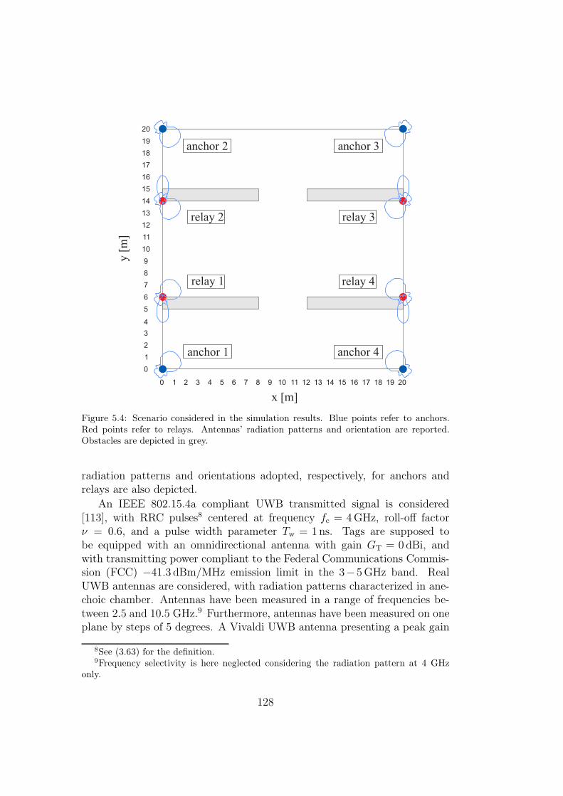
x [m]
y [
m]
anchor 4
relay 4
relay 3
anchor 3anchor 2
relay 2
relay 1
anchor 1
Figure 5.4: Scenario considered in the simulation results. Blue points refer to anchors.Red points refer to relays. Antennas’ radiation patterns and orientation are reported.Obstacles are depicted in grey.
radiation patterns and orientations adopted, respectively, for anchors andrelays are also depicted.
An IEEE 802.15.4a compliant UWB transmitted signal is considered[113], with RRC pulses8 centered at frequency fc = 4GHz, roll-off factorν = 0.6, and a pulse width parameter Tw = 1ns. Tags are supposed tobe equipped with an omnidirectional antenna with gain GT = 0dBi, andwith transmitting power compliant to the Federal Communications Commis-sion (FCC) −41.3 dBm/MHz emission limit in the 3−5GHz band. RealUWB antennas are considered, with radiation patterns characterized in ane-choic chamber. Antennas have been measured in a range of frequencies be-tween 2.5 and 10.5 GHz.9 Furthermore, antennas have been measured on oneplane by steps of 5 degrees. A Vivaldi UWB antenna presenting a peak gain
8See (3.63) for the definition.9Frequency selectivity is here neglected considering the radiation pattern at 4 GHz
only.
128

GA=5dBi and a half power beam width (HPBW) of 101 degrees is adoptedfor anchors and relay’s antenna A (tag-relay links) [266]. A four-patch ar-ray antenna presenting a peak gain GA=12 dBi and a HPBW of 45 degreesis considered as the relay’s antenna B (relay-anchor links) [267]. Antennasmeasurements have stressed out how some antennas features, such as theradiation pattern, could drive the choice of adopting an antenna instead ofanother in a localization context.
Anchors have a noise figure F = 5 dB. Additive noise at relays shouldin principle be taken into account. The extra noise power radiated by therelay scales with GFR − 1, where G and FR have been defined in Sec. 5.2.1.However, when received by an anchor, this power is attenuated by the path-loss between the anchor and the relay. When putting realistic figures, itturns out that in most practical cases the relay noise power received by ananchor is well below the anchor additive noise and is therefore negligible.Consequently, it is Ni,m ≪ N0, and hence Ni,m, for i 6= 0, are neglected inthe following simulation results.
In order to show the performance of the relay-based localization in differ-ent propagation conditions, two dense multipath models [102, 56] are adoptedfor the tag-anchor and tag-relay channels, considering a rms channel delayspread of 1.5 ns (softer multipath) and of 5 ns (stronger multipath), respec-tively. In both cases we consider an exponential PDP with paths separated of1.5 ns apart, a probability b=0.7 of having a path, each path with Nakagamifading (severity factor m=3) except for the first-path taken as determinis-tic according to the free-space path loss model (β = 2).10 Due to the highdirectivity of the relay antenna oriented in the anchor direction, an AWGNrelay-anchor channel is considered.
Unless differently reported, a total of Ns=256 pulses is considered in theranging packet with a PRP Tf = 100 ns. Ideal knowledge of the delay t0 isassumed.
10This is, obviously, a best-case assumption since also the first-path (i.e., the directone) expresses a variance with respect to the deterministic free-space propagation model.However, recently it has been shown how the RSSI measurements performed on UWBsignals can lead to an accurate distance estimation, thanks to the capability of mitigatingfading effects [268, 269]. This estimation capability is a consequence of the small varianceexperienced by the first path with respect to an ideal propagation condition, motivationof our choice of this deterministic value (furthermore the obtained performance can beintended as a performance limit).
129

5.4.2 Performance Metrics
Results have been obtained with Monte Carlo simulations considering thetags uniformly and equally-spaced distributed in the monitored area. Inparticular a 50 cm grid, resulting in the set of positions pn, n = 1, . . . , N ,has been defined in the environment, which points are adopted as potentialtag locations and test locations for position estimation.
As performance indicator we adopt the localization error outage (LEO),defined as the rate at which the localization error is greater than a giventarget error eth [138, 28] (i.e., the fraction of spatial test locations that donot fulfill a target error requirement), that is
LEO =1
N
N∑
n=1
1R+(e (p)− eth) (5.45)
where we have defined the indicator function 1A(x)=1 if x ∈ A, 0 otherwise,and e (p) is the localization error in the nth test position of the grid. TheRMSE is adopted as error metric e (p) output of the Monte Carlo simulation,that is
e (p) =
√√√√ 1
M
M∑
m=1
e2m (p) (5.46)
where the localization error related to the mth iteration em (p) is the Eu-clidean distance between the estimated position pm and the true position,that is em (p) = ||pm − p||, and M is the number of simulation iterations.LEO is presented as function of the relay gain G, assumed the same for allthe relays present in the environment (i.e., Gi = G ∀i = 1, . . . , Nr). Resultsare provided considering a target error eth=50 cm.
The c.d.f.s of the RMSE, and the RMSE itself in the two-dimensional(2D) environment are also reported for selected configurations. Each c.d.f.represents the ratio between the number of test locations for which the RMSEis lower or equal than a specific value and the total amount of test locationsin the grid.
5.4.3 Simulation Results
Figure 5.5 reports the LEO for the softer multipath channel. In particularthe violet curve (�) refers to the estimator A (5.10). Blue curve (◦) refers tothe estimator B1 (5.28), yellow curve (△) refers to the estimator B2 (5.36),while the red curve (⋄) refers to the estimator B3 (5.44). Estimator A andestimator B1 have been implemented according to a sub-optimal, and more
130
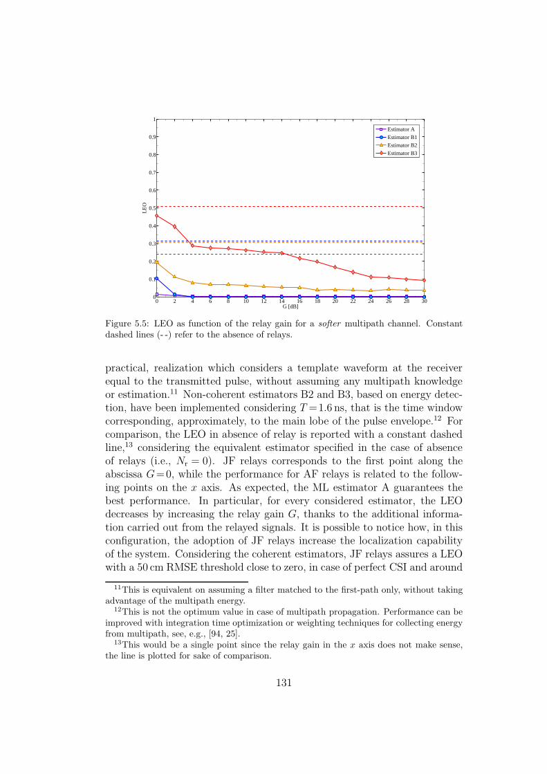
0 2 4 6 8 10 12 14 16 18 20 22 24 26 28 300
0.1
0.2
0.3
0.4
0.5
0.6
0.7
0.8
0.9
1
G [dB]
LEO
Estimator A
Estimator B1
Estimator B2
Estimator B3
Figure 5.5: LEO as function of the relay gain for a softer multipath channel. Constantdashed lines (- -) refer to the absence of relays.
practical, realization which considers a template waveform at the receiverequal to the transmitted pulse, without assuming any multipath knowledgeor estimation.11 Non-coherent estimators B2 and B3, based on energy detec-tion, have been implemented considering T =1.6 ns, that is the time windowcorresponding, approximately, to the main lobe of the pulse envelope.12 Forcomparison, the LEO in absence of relay is reported with a constant dashedline,13 considering the equivalent estimator specified in the case of absenceof relays (i.e., Nr = 0). JF relays corresponds to the first point along theabscissa G=0, while the performance for AF relays is related to the follow-ing points on the x axis. As expected, the ML estimator A guarantees thebest performance. In particular, for every considered estimator, the LEOdecreases by increasing the relay gain G, thanks to the additional informa-tion carried out from the relayed signals. It is possible to notice how, in thisconfiguration, the adoption of JF relays increase the localization capabilityof the system. Considering the coherent estimators, JF relays assures a LEOwith a 50 cm RMSE threshold close to zero, in case of perfect CSI and around
11This is equivalent on assuming a filter matched to the first-path only, without takingadvantage of the multipath energy.
12This is not the optimum value in case of multipath propagation. Performance can beimproved with integration time optimization or weighting techniques for collecting energyfrom multipath, see, e.g., [94, 25].
13This would be a single point since the relay gain in the x axis does not make sense,the line is plotted for sake of comparison.
131
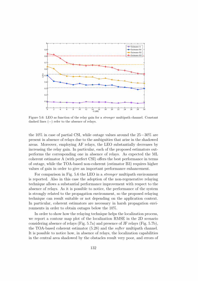
0 2 4 6 8 10 12 14 16 18 20 22 24 26 28 300
0.1
0.2
0.3
0.4
0.5
0.6
0.7
0.8
0.9
11
G [dB]
LEO
Estimator A
Estimator B1
Estimator B2
Estimator B3
Figure 5.6: LEO as function of the relay gain for a stronger multipath channel. Constantdashed lines (- -) refer to the absence of relays.
the 10% in case of partial CSI, while outage values around the 25−30% arepresent in absence of relays due to the ambiguities that arise in the shadowedareas. Moreover, employing AF relays, the LEO substantially decreases byincreasing the relay gain. In particular, each of the proposed estimators out-performs the corresponding one in absence of relays. As expected the MLcoherent estimator A (with perfect CSI) offers the best performance in termsof outage, while the TOA-based non-coherent (estimator B3) requires highervalues of gain in order to give an important performance enhancement.
For comparison in Fig. 5.6 the LEO in a stronger multipath environmentis reported. Also in this case the adoption of the non-regenerative relayingtechnique allows a substantial performance improvement with respect to theabsence of relays. As it is possible to notice, the performance of the systemis strongly related to the propagation environment, so the proposed relayingtechnique can result suitable or not depending on the application context.In particular, coherent estimators are necessary in harsh propagation envi-ronments in order to obtain outages below the 10%.
In order to show how the relaying technique helps the localization process,we report a contour map plot of the localization RMSE in the 2D scenarioconsidering absence of relays (Fig. 5.7a) and presence of JF relays (Fig. 5.7b),the TOA-based coherent estimator (5.28) and the softer multipath channel.It is possible to notice how, in absence of relays, the localization capabilitiesin the central area shadowed by the obstacles result very poor, and errors of
132

x [m]
y [m
]
0 2 4 6 8 10 12 14 16 18 200
2
4
6
8
10
12
14
16
18
20
0
2
4
6
8
10
12
14
RMSE [m]
(a) Without relays
x [m]
y [m
]
0 2 4 6 8 10 12 14 16 18 200
2
4
6
8
10
12
14
16
18
20
0
2
4
6
8
10
12
14
RMSE [m]
(b) JF relays
Figure 5.7: RMSE contour map in the 2D environment.
several meters can occur due to the lack of anchors visibility. Differently, theadoption of non-regenerative AF relays allows extending the system coveragein the shadowed areas, ensuring enhanced localization performance.
The performance improvement can be shown also in terms of c.d.f. of thelocalization error. Figure 5.8 shows the results considering absence of relays(in dashed lines) as well as presence of JF relays (in continuous lines), and AFrelays with G=10 dB (in dot-dashed lines) for the softer multipath channel.Again, the adoption of relaying assures a benefit in terms of the number ofspatial points that can be localized with a target location accuracy withoutambiguity.
The presented results proved the effectiveness of the relaying techniquefor network localization. In the proposed configuration the adoption of bothJF and AF produce important benefits.
5.5 Conclusion
The idea of UWB non-regenerative relays for network localization has beenintroduced as a low complexity solution to increase the service coverage inhigh-definition RTLS based on UWB technique when operating in severeNLOS propagation conditions. The adoption of JF or AF relays increases thenumber of received signal components that, thanks to the a priori knowledgeof relay positions, contribute in decreasing the possibility of ambiguities inML estimators. Thus the relays act as additional virtual anchors. Numericalresults show that significant performance improvement can be achieved, evenusing simple passive JF relays, with respect to the absence of relays. UWB
133

Figure 5.8: c.d.f.s of the RMSE. Dashed lines (- -) refer to the absence of relays, continuouslines (–) refer to the presence of JF relays, dot-dashed lines (· -) refer to the presence ofAF relays.
non-regenerative relays can also be adopted to reduce the number of anchorswith consequent reduction of the network infrastructure cost and complexity.
5.A Derivation of the ML estimator
The ML estimate a(m) of a(m) can be easily obtained via LS [161, ch. 8] as
a(m) = W(m)+(p)r(m) (5.47)
whereW(m)+(p) =
(W(m)
T (p)W(m)(p))−1
W(m)T (p) is the Moore-Penrose pseudo-
inverse matrix [265, p. 421]. Sobstituting (5.47) in (5.21) and neglecting theterm not function of p we obtain
p =argmax(p,t0)
{Na∑
m=1
1
2σ2m
(2 r(m)TW(m)(p)W(m)
+(p)r(m)
−∥∥W(m)(p)W(m)
+(p)r(m)∥∥2)}
. (5.48)
134

Considering that14
∥∥W(m)(p)W(m)+(p)r(m)
∥∥2 = r(m)TW(m)(p)W(m)+(p)r(m) (5.49)
the final form of (5.48) is
p =argmax(p,t0)
{Na∑
m=1
1
2σ2m
χ(m)T (p) R(m)
−1(p) χ(m)(p)
}(5.50)
where
χ(m)(p) = W(m)T (p) r(m)
=[w(m)T
D1,m(p)r(m),w(m)T
D2,m(p)r(m), . . . ,w(m)T
DL,m(p)r(m)]∈ R
L
(5.51)
is the vector of correlation between the received signal and the delayed ver-sions of the template pulses gl
(m), and
R(m)(p) = W(m)T (p)W(m)(p)
=
w(m)T
D1,m(p)w(m)D1,m(p) w(m)T
D1,m(p)w(m)D2,m(p) · · · w(m)T
D1,m(p)w(m)DL,m(p)
w(m)T
D2,m(p)w(m)D1,m(p) w(m)T
D2,m(p)w(m)D2,m(p) · · · w(m)T
D2,m(p)w(m)DL,m(p)
......
. . ....
w(m)T
DL,m(p)w(m)D1,m(p) w(m)T
DL,m(p)w(m)D2,m(p) · · · w(m)T
DL,m(p)w(m)DL,m(p)
(5.52)
is the cross-correlation matrix of the template pulses.
5.B Derivation of the ML estimator
The ML estimate g of g can be obtained adopting the LS technique [161, ch.8] as
g =
√ET
H(m)+(p)r(m)
‖H(m)+(p)r(m)‖ (5.53)
whereH(m)+(p) =
(H(m)
T (p)H(m)(p))−1
H(m)T (p) is the Moore-Penrose pseudo-
inverse matrix [265, p. 421], and the normalization is imposed in such a way
14Proof of (5.49)Considering that ‖x‖2 = xTx, and posing Ξ = W(m)(p)W(m)
+(p), we have ‖Ξr(m)‖2 =
r(m)TΞTΞ r(m). Since Ξ is an orthogonal projection matrix [161, pag. 231], that is, a
symmetric (ΞT =Ξ) and idempotent (Ξ2=Ξ) matrix, we obtain directly (5.49).
135

the estimate is consistent according to the transmitted energy assumption‖g‖2 = ET . Substituting (5.53) in (5.33) and neglecting the terms not de-pendent on p we obtain
p =argmax(p,t0)
{Na∑
m=1
1
2σm
(2
√ET
r(m)TH(m)(p)H(m)+(p)r(m)
∥∥H(m)+(p)r(m)
∥∥
− ET
∥∥H(m)(p)H(m)+(p)r(m)
∥∥2∥∥H(m)
+(p)r(m)∥∥2
)}. (5.54)
Considering that (same proof of 5.A-(5.49) considering H(m)(p) instead ofW(m)(p))
∥∥H(m)(p)H(m)+(p)r(m)
∥∥2 = r(m)TH(m)(p)H(m)+(p)r(m) (5.55)
we get the expression (5.34).
5.C Derivation of the ML estimator
In the case of not overlapped replicas matrix H(m)(p) takes the form of ablock matrix
H(m)(p) =
0D1,m(p),M
H(m)1 (p)
0D2,m(p)−D1,m(p)−M,M
H(m)2 (p)...
H(m)L (p)
(5.56)
where H(m)i (p) = ai,m(p)IM , i = 1, . . . , L, are M×M scalar matrices. Ex-
ploiting the property of block matrix product, the block H(m)T (p)H(m)(p) in
(5.34) takes the form
H(m)T (p)H(m)(p) =
L∑
l=1
H(m)l
2(p) =
L∑
l=1
a2l,m(p) IM . (5.57)
Consequently we can define the scalar matrix D =(H(m)
T (p)H(m)(p))−1
with
non zero elements on the main diagonal equals to(∑L
l=1 a2l,m(p)
)−1
. It is so
136

possible to rewrite (5.35) as
E (m)(p) = r(m)TH(m)(p)DH(m)T (p)r(m)
=1
∑Ll=1 a
2l,m(p)
r(m)TH(m)(p)H(m)T (p)r(m)
=1
∑Ll=1 a
2l,m(p)
∥∥∥r(m)TH(m)(p)∥∥∥2
. (5.58)
It is now easy to show that
∥∥∥r(m)TH(m)(p)∥∥∥2
=
L∑
i=1
L∑
j=1
ai,m(p) aj,m(p)
M−1∑
n=0
r(m)Di,m(p)+n r
(m)Dj,m(p)+n (5.59)
and consequently
E (m)(p) =1
∑Ll=1 a
2l,m(p)
L∑
i=1
L∑
j=1
ai,m(p) aj,m(p)
M−1∑
n=0
r(m)Di,m(p)+n r
(m)Dj,m(p)+n .
(5.60)
With similar considerations and operations on block matrices, it is pos-
sible to show that∥∥H(m)
+(p)r(m)∥∥2 in (5.54) takes the form
∥∥H(m)+(p)r(m)
∥∥2 = 1(∑L
l=1 a2l,m(p)
)2L∑
i=1
L∑
j=1
ai,m(p) aj,m(p)
×M−1∑
n=0
r(m)Di,m(p)+n r
(m)Dj,m(p)+n . (5.61)
By substituting (5.60) and (5.61) in (5.34) the following formulation of theestimator is obtained
p =argmax(p,t0)
{Na∑
m=1
1
2σ2m
[2
(ET
L∑
i=1
L∑
j=1
ai,m(p) aj,m(p)
M−1∑
n=0
r(m)Di,m(p)+n r
(m)Dj,m(p)+n
)1/2
− ET
L∑
l=1
a2l,m(p)
]}. (5.62)
137

This estimator has an immediate continuous-time equivalent as
p =argmax(p,t0)
{Na∑
m=1
1
Nm
[2
(ET
L∑
l=1
a2l,m(p)
∫ τl,m(p)+Tp
τl,m(p)
r2m(t) dt
+
L∑
i=1
L∑
j=1,j 6=i
ai,m(p) aj,m(p)
∫ Tp
0
rm(t− τi,m(p)) rm(t− τj,m(p)) dt
)1/2
−ET
L∑
l=1
a2l,m(p)
]}. (5.63)
If now we make the assumption15
rm(t− τi,m(p)) ≃ai,m(p)
aj,m(p)r(t− τj,m(p)) for t ∈ (0, Tp) (5.64)
we have that (5.63) simplifies to
p =argmax(p,t0)
{Na∑
m=1
1
Nm
(2
√√√√ET
L∑
l=1
a2l,m(p)
L∑
k=1
∫ τk,m(p)+Tp
τk,m(p)
r2m(t) dt
−ET
L∑
l=1
a2l,m(p)
)}. (5.65)
By considering that ET
∑Ll=1 a
2l,m(p) is the overall received energy E(m)(p)
from a tag in position p at the anchor m, collected considering the L replicas,we get the final estimator form
p = argmax(p,t0)
{Na∑
m=1
1
Nm
(2
√E(m)(p)
∫
D(m)(p)
r2m(t) dt− E(m)(p)
)}(5.66)
where we have indicated with
D(m)(p) ={(τ1,m(p, t0), τ1,m(p, t0) + Tp) ∪ (τ2,m(p, t0), τ2,m(p, t0) + Tp) ∪ . . .
∪ (τL,m(p, t0), τL,m(p, t0) + Tp)}
(5.67)
the set of time intervals in which replica contributions are expected whentag’s position p is under hypothesis.
Notice that in this case the estimator takes advantage of the knowledgeof the expected received energy for each replica, through the vector (5.16), so
15This assumption is verified with increasing confidence while increasing the SNR.
138

in the formulation (5.66) it would be expected that the energy measurementsrelated to replicas corresponding to w(·, ·) = 0 were discarded. Conversely in(5.66) the energy measurement is performed on the overall set of L replicas,also if some of these do not carry useful signal contribution. The problemarises due to the approximation (5.64): in fact, in the exact formulation ofthe estimator in (5.63) each correlation and energy measurement is properlyweighted and discarded if related to replicas with w(·, ·) = 0 (i.e., replicasnot effectively present at the receiver.). Therefore, in order to maximizethe performance for the simplified implementation (5.66) it is important torestrict the integral extremes at only the windows where, for each hypothesis,we effectively expect useful signal, in order to not add noise or interferencecontributions. This can be accounted for by adopting D(m)(p), defined in(5.37), instead of D(m)(p) in (5.66), leading to (5.36).
139

140

Part IV
A Case-Study: TheUWB-RFID System
141


Introduction
One of the more interesting applications of context-aware networks is relatedto the possibility of monitoring environments, such as security areas or fac-tories, in this second case mainly in order to increase the efficiency of thelogistic process. In fact, in recent years, a significant number of industrialrealities have moved towards the so-called supply chain management (SCM)approach [270], relying on the administration of the various logistics aspectsof the company. One of the main requirements of the SCM approach is thevisibility of the goods along the chain. More precisely, it is necessary to knowwhat a given object is (the who question), and where it can be found (thewhere question) at a given instant in time (the when question). Existingautomatic identification (AI) technologies (e.g., bar codes or RFID) and theRTLS are not able to provide a complete solution. In fact, both of themsuffer from significant limitations. On the one hand AI systems are ableto answer to the “who” question, but they are weak on the “where” ques-tion. To obtain the complete item visibility, items have to be scanned anda position information must be manually inserted or read from a separatesource (e.g., another tag). These aspects severely reduce the efficiency ofSCM and introduce uncertainty because of manual operations. On the otherhand, RTLS satisfy mainly the location requirement, but fail to manage theidentification requirement when the item is out of the RTLS working area.Moreover, the current generation of RTLS is based on active tags. This leadsto two deficiencies: a limited battery lifetime and a high cost of the tag. As aconsequence, the wide spreading of RTLS systems is still not fully exploited.
Recently it has been shown that IR-UWB is a very promising technique,which could meet the stringent requirements of passive tag localization interms of accuracy [50]. In [271] a passive UWB-RFID scheme has been pro-posed, showing its potential operating range/data rate trade-off. The advan-tage of such a technology is to provide the typical accuracy of UWB-RTLSby employing a very simple tag, which adopts backscattering modulationinstead of using a complete UWB active transmitter. However one of themost important issues in these systems is the energy supply. CombiningUWB (semi-)passive RFID with already existing UHF technologies can be apossible solution to exploit energy harvesting [272] or to implement wake-upstrategies in order to increase the battery life of semi-passive tags. More-over the UHF module can be employed to ensure compatibility with alreadyexisting RFID systems working in the UHF band.
In this last part of the thesis the study of a UHF-UWB semi-passive RFIDsystem is presented as example of possible context-aware network solutionwhich enables localization and tracking features. Chapter 6 introduces the
143

system concept providing an overview of the main features and issues relatedto the realization of such a network. Chapter 7 investigates the feasibil-ity of the system from the signal demodulation point of view, highlight-ing particular characteristics and signal processing techniques for dealingwith impairments such as the clutter. Chapter 8 analyzes the problem ofmulti tag interference providing design guides of solution able to counteractthese effects, also in presence of hardware non idealities. Finally, Chap-ter 9 focuses on the localization aspect deriving the fundamental limits onthe achievable accuracy adopting this kind of system. The work has beencarried out in the context of the European project SELECT.16 The scopesof the project are related to the investigation of this new technology ableof combining functionalities of detection, identification and localization byfusing the concept RFID based on backscatter modulation, and adoptingsemi-passive tags, and RTLS. In additions sensing capabilities are supposedto be provided by the networks thanks to the adoption of WSR techniques[273, 274, 275, 276, 277, 278, 279, 280, 281] for detection and tracking ofuntagged objects.
16www.selectwireless.eu
144

Chapter 6
System Overview
6.1 Introduction
We consider here a UWB-RFID system composed of a network of readersmonitoring an area where tags are present. In particular tags are semi-passiveand based on backscatter modulation, where the low energy available fromharvesting or batteries is used only for memory access or modulation opera-tion without powering an active transmitter. The high accuracy estimation ofthe TOA from the backscatter signals enables accurate localization of tags inaddition to their detection [50, 136, 51]. The joint use of the RFID and UWBtechnology is an appealing solution, as UWB leads to advantages in terms ofcommunication robustness, localization accuracy, multi-tag capability, evenin harsh propagation environments [53, 48].
Figure 6.1 shows an example of such an architecture. In particular thenetwork of readers cover a scenario where several tagged objects are present.Readers act as reference nodes and are placed in known positions. Theyare the only active entity capable of transmitting, receiving and processingsignals. The goal of the network is detect the presence of tagged objects bythe analysis of the response (i.e., the backscatter) of the tags. Moreover,in addition to the detection, high-accuracy localization, enabled by TOAestimation, is performed by the readers’ network to locate tagged objects.The passive link between the tag and the reader can be also exploited totransmit information between these two entities, for example the tag ID ordata collected by sensors attached to tags. In addition, the same readersinfrastructure is exploited as a radar sensor network (RSN) to detect andlocate untagged entities (i.e., passive scatters) not equipped with tags [50,274, 282]. This is possible adopting radar techniques able to track the changesin the environment response caused by the movement of untagged objects.
145

Figure 6.1: Application scenario.
The standard application scenario, composed a square cell monitored by fourreaders is depicted in Fig. 6.2.
6.2 UWB Backscattering Principle
Backscatter communication is based on the modulation of the interrogationsignal emitted by a reader. This modulation, operated by a tag, is realizedby changing the load connected to the tag antenna [4].
An example of the received signal at reader side, when backscatter mod-ulation at tag side is adopted, is shown on Fig. 6.3, where the receivedbackscatter signal for three states of the load impedance ZL connected tothe tag antenna is presented. In one of them (black), the load is 50 Ohms,which equals the antenna internal impedance. In this case, the backscattersignal is called structural mode and is dominated by the physical structureof the antenna and its various parts. In the two other cases, we distinctlysee that a portion of the signal depends on the load impedance. This part ofthe backscatter signal is named antenna mode and it is the one that allowsdifferential detection through the tag load impedance state.
The round trip backscatter CIR is the result of the convolution betweenthe reader-tag propagation CIR convoluted by itself and the backscatter an-tenna mode response of the tag. The contours of a complete backscatterchannel model encompassing all these contributions have been described in[283]. The UWB round trip backscattering channel is strongly unfavorablefrom the energetic point of view, since the received backscattered signal ex-periences pathloss between the reader and the tag twice. Basically, similarlyto the radar equation, the distance-dependence of the received signal powerscales, in free space, with the 4th power of the reader-tag distance, whichmeans a detection distance much smaller than for an ordinary communica-
146

Figure 6.2: Example of a square cell monitored by four readers.
tion link. It is important to underline that the tag backscattering behavioris strongly impacted by the presence of the object on which it is attached[284]. Together with the tag response the reader receives the signal reflectedby the surrounding environment, that is the clutter component. A schemeof these propagation effects is reported in Fig. 6.4.
6.3 System Architecture and Main Function-
alities
The overall RFID network architecture is depicted in Fig. 6.5. It comprisesa central unit, readers and tags. Moreover, relay nodes, that are devicesunconnected to the wired core network, can be incorporated herein [30].1
Each reader communicates with the central unit mostly for transferring thesignal processing data (e.g., the TOA estimate allowing the tag positioning).In addition these wired connections can be exploited in order to ensure ageneral coarse synchronization between the readers, as well as for network
1These are, for example, the relays described in Chapter 5.
147

Figure 6.3: Example of backscattered signal, for three tag load impedance values (freespace).
maintenance. Reader synchronization will be further detailed in Sec. 6.3.2.
In Fig. 6.6 and Fig. 6.7, the architecture proposed in [271] and analyzedin [285] for UWB readers and tags adopting backscatter modulation is re-ported. This architecture represents the UWB core enabling the backscat-tering scheme for localization and tracking.
In particular, the reader is composed of a transmitter and a receiversection. During the interrogation cycle, the reader transmits a sequenceof UWB pulses modulated by a periodic binary spreading sequence {dn} ofperiodNc with dn ∈ {−1, 1}, specific of that particular reader (reader’s code).In general, Npc pulses are associated to each code symbol (chip) of durationTc seconds. To accommodate the signals backscattered by tags correspondingto an entire packet of Nr bits, the UWB interrogation contains Nt = NrNs
pulses, where Ns = NcNpc is the number of pulses associated to each bit.Pulses are separated by Tp seconds, thus the chip time is Tc = Npc Tp. Eachtransmitted pulse is backscattered by the tag’s antenna as well as by all thesurrounding scatterers present in the environment which form the cluttercomponent.
In Fig. 6.6, an example of UWB tag architecture employing a binarybackscatter modulator composed of an UWB switch is shown. The switch
148

(depends on the tag load)
y
zz
y
x
rφt
ϑtr
Z LREADER
1
backscatter signal (clutter)
TAG
CLUTTER
a (f)
b (f)
1
tag reference systemreader reference system
φ
ϑ
structural mode scattering
antenna mode scattering
x
Figure 6.4: Signal contributions at the reader port [285].
is controlled by a micro-controller whose purpose is to change the switchstatus (short or open circuit) at each chip time Tc according to the data tobe transmitted and a zero mean (balanced) periodic tag’s code {cn}, withcn ∈ {−1,+1}, of period Nc. The adoption of balanced codes ensures theremoval of the clutter as will be demonstrated in Chapter 7 and Chapter 8.Specifically, each tag information bit bk ∈ {−1,+1} is associated toNs pulses,thus the symbol time becomes Ts = TcNc = Tp Ns. In this way the polarityof the reflected signal changes according to the tag’s code during a symboltime, whereas the information symbol (bit) affects the polarity of all pulsescomposing the sequence each symbol time.
By analyzing the received signal components shown in Fig. 6.8, it can benoted that the antenna mode scattered component only is modulated by thecombination of the tag’s and reader’s codes {cn} and {dn}, whereas all cluttersignals components (included the antenna structural mode scattering) arereceived modulated by the reader’s code {dn} only. This property is exploitedat the reader receiver section to remove the clutter component through aproper processing, therefore isolating the useful component coming from theintended tag. The presented MAC scheme is fundamentally a direct-sequencecode division multiple access (CDMA) approach, according to which a de-spreading phase at reader side can be exploited to detect and demodulatea specific tag signal. However, several issues arise due to tag multi-userinterference (MUI) and near-far effects, as will be presented in Chapter 8.
An example of possible receiver scheme is that reported in Fig. 6.6 wherea correlator-based demodulator is considered. This scheme performs a de-spreading operation (i.e., the accumulation of the Ns pulses composing a
149

Figure 6.5: SELECT general system architecture.
symbol) using the combined code {cn · dn}, which identifies both the readerand the desired tag.
Several signal processing tasks have to be accomplished by the readers inorder to provide to the RFID network detection and localization capabilities.In particular the first task consists of tag detection, that is the process thanksto which the network knows that a certain tag is present in the monitoredarea. When tags multiple access is performed with CDMA and a certainspreading code is uniquely assigned to a tag, a decision at the output to thede-spreading phase is sufficient to accomplish the identification purpose. Ifthe network aim is only confined to detection and localization, the secondtask to be accounted is related to TOA estimation, thanks to which local-ization capabilities are provided. If the tag itself has data to transmit tothe reader (e.g., because it has an embedded sensor, or data related to theobject to which it is attached, or because the spreading code associated to itis not unique), the reader must perform signal demodulation in addition todetection.
As already mentioned, TOA estimation enables localization capabilities,thanks to the location estimation process realized at central unit by fusingthe data provided by at least three readers. For this kind of system, dueto the low complexity of the tag and to the fact that tags cannot directlycommunicate, no cooperative techniques can be exploited for performanceimprovement and coverage extension, so that every point of the monitored
150

n{d }
pulse
generatorseq. generator
transmitter
Detector
decoded
receiver
Despreader
reader code
symbols
READER
RX antenna
TX antenna
w (t) templateref
{d }
{c }n tag code
reader code
n
Figure 6.6: UWB reader architecture in backscattering schemes [271].
area must be directly covered by a sufficient number of readers.2
The most interesting unique feature of the UWB-RFID network is relatedto the possibility of performing all these functionalities, tag detection, signaldemodulation, TOA estimation and location determination, not only readerby reader as independent entities, but at network level, providing an inherentdiversity. Some examples will be provided in the following sections.
6.3.1 Tags Synchronization
Tags synchronization is a fundamental task allowing several benefices in theUWB-RFID system. In fact, if tags code generators are completely free-running, the reader must perform an exhaustive code acquisition search inorder to synchronize its code generator used for de-spreading with the incom-ing tag signal. A (partial) synchronization of the system allows exploitingparticular codes families able to better mitigate the multi-user interference(see Chapter 8). To accomplish this task, the UHF link3 can be used toderive the synchronization signal necessary to reset the tags’ spreading codegenerators.
Specifically, according to Fig. 6.9 the reset of the tag code generator isperformed on the falling edge of a wake up UHF carrier received by the tags.This signal enables powering up a UHF circuit by charging a capacitor viathe antenna and a rectifier circuit. The resulting voltage is used to power acontrol circuit that, at the time the transmission of the continuous wave (CW)signal has ended, activates the switch via powering its control logic from the
2Also relaying techniques can be adopted as presented in Chapter 5.3We consider a hybrid solution including both UWB and standard UHF readers and
tags.
151

switch
energy harvesting
wake−up
circuit
data
spread code
memory
f
n
control logic
fmemorydata (ID)
battery
chip
XORm(t)
antenna
wake−up
{c }
Figure 6.7: UWB tag architecture in backscattering schemes [271].
battery, thus, initiating the backscatter modulation of the UWB signals. Inthis way the propagation-dependent capacitor charge time4 does not play asignificant role in the synchronization jitter, since the discharge starting eventis not affected by the pathloss and depends only on the tags’ positions andorientations. This wake-up synchronization process is depicted in Fig. 6.10.
6.3.2 Readers Synchronization
Readers must be kept synchronized in order to ensure satisfactory MAC per-formance (presented in Sec. 8.6.2) and to allow multistatic functionalities thatwill be described in the following sections. Readers coarse synchronizationcan be provided with the wired readers-central unit links (realized, e.g., witha standard Ethernet protocol). Readers fine synchronization can be basedon UWB signals by re-using the same hardware developed for tag detection.In fact the direct reader-to-reader link, associated with the de-spreading per-formed accumulating a number of pulses Ns, ensures a very high SNR for thedemodulation of the interfering reader signal, allowing very accurate (sub-nanosecond), TOA estimation. In this case the de-spreading is operatedaccording to the incoming reader’s code. Since the reader-reader distance is
4This is due to the narrowband UHF signals that may experience selectively channels,and to different reader-tag distances.
152

Figure 6.8: Backscatter modulation.
fixed, TOA estimation can be compared with the expected propagation timebetween the two readers’ antennas, adjusting consequently the reader’s clockaccording to the difference between the estimated and expected range. Theprocess can be further iterated until the difference in the clock adjustmentfalls below a threshold, indicating the reached synchronism.
6.3.3 Tag Detection
Generically, tag detection can be realized at each reader if the de-spreadsignal level related to a specific tag code is above a certain threshold. Sincemore than one reader is supposed to perform this de-spreading, the decisionon the tag presence can be taken, instead reader by reader, from the centralunit, by properly combining the different observations.
Moreover, especially in conjunction with time division multiple access(TDMA) readers MAC, each reader can perform the de-spreading also whenan other reader is interrogating the tag, adopting, as de-spreading code, theother reader one combined with the tag code.5 In this manner, if a network ofNR readers is monitoring a certain area (e.g., NR = 4 in our square referencescenario), up to N2
R observations can be combined for robust tag detection.
5This requires a synchronous readers network.
153

Figure 6.9: Wake-up scheme.
Figure 6.10: UHF-UWB interrogation cycle.
The analysis of tag detection strategies and performance analysis, con-sidering a single reader, will be presented in Chapter 8.
6.3.4 Signal Demodulation
Signal demodulation allows data communication between tags and readers.In this manner the tag ID can be transfered to the network or, if the tag hasembedded sensors, the network can receive these data.
As for the tag detection, also signal demodulation can benefit of the inher-ent diversity provided by the multi-reader architecture. As example, supposethat each reader demodulates the signal of a specific tag. The demodulationresult, with soft or hard decisions, can be then forwarded to the central unitfor a proper combining and to take a final decision on the received mes-sage, enabling improved performance also whitout high rate channel codingstrategies.
The analysis of signal demodulation performance, considering a singlereader, will be presented in Chapter 7.
154

6.3.5 Time of Arrival Estimation
TOA estimation enables the ranging and localization, and it can be operatedwith high precision thanks to the adoption of UWB signals [51]. Diversityin TOA estimation is ensured by the fact that each reader can perform theestimate not only when it is transmitting, but also when other readers aresending their signals. In this manner we are in the presence of a multistaticnetwork similar to that generally adopted in WSR systems, as explained inthe following section.
6.3.6 Localization
The availability of TOA estimates between the different readers allow thecentral unit to properly fuse the data obtaining the position estimate asintersection, as example, of circles and ovals. The fundamental limits for theaccuracy of this technique will be analyzed in Chapter 9.
Moreover, filtering techniques can be adopted for improving the positionestimation when tags are moving.
6.3.7 Untagged Object Detection and Tracking
There is growing on interest in new radar applications, especially for indoorand outdoor monitoring of high-security areas to prevent intruders [282, 286,274, 275, 276, 277, 278]. One of the key features of the UWB-RFID networkis the possibility of providing, with the same readers infrastructure, radarcapabilities, basically detection and tracking of untagged objects in additionto detection, demodulation and localization of tags.
Tracking of moving untagged objects can be realized by analyzing thechanges in the clutter components caused by object movement. To thispurpose the reader has to isolate the clutter component generated by itsown interrogation signal by de-spreading the received signal using only thereader code. Static clutter is usually removed through differential operations[287, 288, 289, 290, 291].
155

156

Chapter 7
Performance Analysis in IdealConditions
7.1 Motivations
Chapter 6 introduced the general concept of UWB-RFID system, presentingan overview and some design and implementation challenges. Here in thischapter the mathematical system description and the performance analysisin realistic conditions but in absence of hardware constraints are presented.In particular the signal structure proposed in [50, 292, 271] for semi-passiveUWB-RFID with clutter suppression is extended to a multi-tag scenario.The potential performance of backscatter RFID communication using UWBsignals is investigated in terms clutter suppression and multiple access ca-pability using both simulated and experimental data obtained in realisticenvironments. A generic correlation-based receiver is here considered, whileperformance analysis in presence of simplified low-complexity non-coherentschemes and hardware impairments will be addressed in Chapter 8.
7.2 Backscatter Communication using UWB
Signals
Consider a scenario where a reader interrogates Ntag tags located in the samearea. In Fig. 7.1 the architectures for tag and reader are shown. The reader iscomposed of a transmitter and a receiver section both connected to the sameUWB antenna through a TX/RX switch. During the interrogation phase,the reader transmits a sequence of UWB pulses, each having energy Ep. An
157

m (t)
reader tag
k
v(t)
TX/RX switch
Matchedfilter
samplern
tag’s code
seq. generator
n
Ns
ym
transmitter
receiver
UWB antenna
switch
reader’s codeseq. generator
n
a
a
UWB antenna
c
pulsegenerator
Figure 7.1: The considered scheme of the tag and the reader composed of a transmitterand a receiver section.
interrogation sequence or Nr symbols is here considered, that is,
sreader(t) =
Nr∑
m=0
s(t−mNcTc) (7.1)
with
s(t) =Nc∑
n=0
dng(t− nTc) (7.2)
and
g(t) =
Npc−1∑
k=0
p(t− kTp) (7.3)
indicating the composite waveform associated to each code symbol (chip) dncomposed of Npc elementary UWB pulses p(t), centered at frequency fc and
with bandwidth W , each of energy Ep =∫ Tp
0p2(t) dt. Moreover, the pulse
energy Ep and the PRP Tp are set to guarantee a radiated spectrum emissioncompliant with the regulation mask (in terms of effective radiated isotropicpower (EIRP)) [293]. The PRP Tp is chosen so that all backscattered signalsare received by the reader before the transmission of the successive pulse,thus avoiding inter-frame interference. In indoor scenario Tp = 50 − 100 nsis usually sufficient for this purpose [92]. In the following of this chapter weconsider for convenience dn as an infinite periodic sequence.
During the transmission of each pulse the antenna is connected to thetransmitter section. It is then kept connected to the receiver section duringthe remaining time until the successive pulse is transmitted. Each pulse in(7.1) is backscattered by all tags as well as by all the surrounding scattererspresent in the environment that form the clutter component. As shown inFig. 7.1, the tag changes its scattering properties by varying the antenna
158
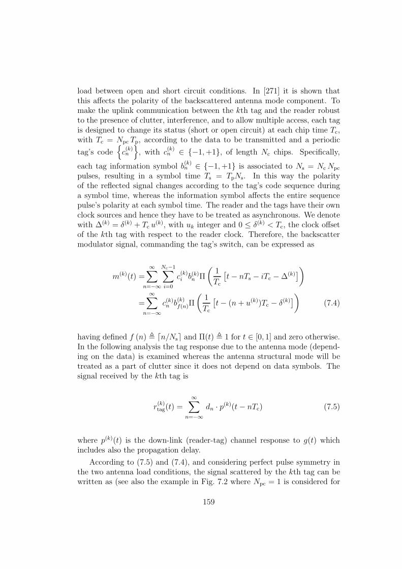
load between open and short circuit conditions. In [271] it is shown thatthis affects the polarity of the backscattered antenna mode component. Tomake the uplink communication between the kth tag and the reader robustto the presence of clutter, interference, and to allow multiple access, each tagis designed to change its status (short or open circuit) at each chip time Tc,with Tc = Npc Tp, according to the data to be transmitted and a periodic
tag’s code{c(k)n
}, with c
(k)n ∈ {−1,+1}, of length Nc chips. Specifically,
each tag information symbol b(k)n ∈ {−1,+1} is associated to Ns = NcNpc
pulses, resulting in a symbol time Ts = TpNs. In this way the polarityof the reflected signal changes according to the tag’s code sequence duringa symbol time, whereas the information symbol affects the entire sequencepulse’s polarity at each symbol time. The reader and the tags have their ownclock sources and hence they have to be treated as asynchronous. We denotewith ∆(k) = δ(k) + Tc u
(k), with uk integer and 0 ≤ δ(k) < Tc, the clock offsetof the kth tag with respect to the reader clock. Therefore, the backscattermodulator signal, commanding the tag’s switch, can be expressed as
m(k)(t) =
∞∑
n=−∞
Nc−1∑
i=0
c(k)i b(k)n Π
(1
Tc
[t− nTs − iTc −∆(k)
])
=
∞∑
n=−∞c(k)n b
(k)f(n)Π
(1
Tc
[t− (n+ u(k))Tc − δ(k)
])(7.4)
having defined f (n) , ⌈n/Ns⌉ and Π(t) , 1 for t ∈ [0, 1] and zero otherwise.In the following analysis the tag response due to the antenna mode (depend-ing on the data) is examined whereas the antenna structural mode will betreated as a part of clutter since it does not depend on data symbols. Thesignal received by the kth tag is
r(k)tag(t) =
∞∑
n=−∞dn · p(k)(t− nTc) (7.5)
where p(k)(t) is the down-link (reader-tag) channel response to g(t) whichincludes also the propagation delay.
According to (7.5) and (7.4), and considering perfect pulse symmetry inthe two antenna load conditions, the signal scattered by the kth tag can bewritten as (see also the example in Fig. 7.2 where Npc = 1 is considered for
159

simplicity)
s(k)tag(t) = r
(k)tag(t) ·m(k)(t)
=∞∑
n=−∞dn
[c(k)
n−u(k)b(k)
f(n−u(k))p(k)I (t− nTc)
+ c(k)
n−u(k)−1b(k)
f(n−u(k)−1)p(k)II (t− nTc)
](7.6)
where we define
p(k)I (t) , p(k)(t) · Π
(t− δ(k)
Tc − δ(k)
), (7.7)
p(k)II (t) , p(k)(t) · Π
(t
δ(k)
). (7.8)
The main task of the receiver section of the reader is to detect the usefulbackscattered signal component (i.e., the antenna mode scattering dependenton antenna load changes) from those backscattered by the antenna structuralmode and other scatterers (clutter) that are, in general, dominant [271]. Thereceived signal at the reader is
rreader(t)=
Ntag∑
k=1
r(k)reader(t) +
∞∑
n=−∞dnw
(C)(t− nTc)+n(t) , (7.9)
where n(t) is the AWGN with two-sided power spectral density N0/2 andw(C)(t) is the backscattered version of the waveform g(t) due to the cluttercomponent which also accounts for pulse distortion, multipath propagation,and tag’s antenna structural mode. The signal r
(k)reader(t) represents the re-
ceived useful component due to the kth tag, that is,
r(k)reader(t) =
∞∑
n=−∞dn
[c(k)
n−u(k)b(k)
f(n−u(k))w
(k)I (t− nTc)
+ c(k)
n−u(k)−1b(k)
f(n−u(k)−1)w
(k)II (t− nTc)
](7.10)
having denoted w(k)I (t) and w
(k)II (t), respectively, the uplink channel response
to p(k)I (t) and p
(k)II (t) (see Fig. 7.2). Note that w(k)(t) = w
(k)I (t) + w
(k)II (t) is
the round-trip response to g(t) of the backscatter link.
160

preader
(t)
a0 a1
p (t)I
tags (t)
m(t)
δ
Iw (t)
t
t
r (t)tag
c
t
t
t
+1 d
−1
p (t)II
reader(t)r
w (t)II
−n −n/Ns
Ts
Figure 7.2: The behavior of the signals described in section 7.2.
7.3 Multiple Users Interference and Clutter
Consider the reader’s receiver scheme reported in Fig. 7.1 where the re-ceived signal is correlated with a local composite waveform template h(t)with unitary energy. The output is then sampled at sampling intervalsti,m = i Tc +mTs + τ0, with i = 0, 1, ..., Ns − 1 and where τ0 accounts for the
161
propagation delay, thus obtaining the samples
vi,m =
∫ Tc
0
h(t) rreader(t− ti,m) dt = rreader(ti,m)⊗ h(−ti,m)
=
Ntag∑
k=1
v(k)i,m + v
(C)i,m + zi,m (7.11)
where
v(k)i,m=
∞∑
n=−∞dn
[c(k)
n−u(k)b(k)
f(n−u(k))γ(k)I (iTc +mTs + τ0 − nTc)
+ c(k)
n−u(k)−1b(k)
f(n−u(k)−1)γ(k)II (iTc +mTs + τ0 − nTc)
](7.12)
and
v(C)i,m =
∞∑
n=−∞dnγ
(C)(iTc +mTs + τ0 − nTc) . (7.13)
In (7.11) and (7.12) we have defined γ(k)I (t) , w
(k)I (t) ⊗ h(−t), γ
(k)II (t) ,
w(k)II (−t) ⊗ h(−t),γ(C)(t) , w(C)(t)⊗ h(−t), z(t) , n(t)⊗ h(−t), and zi,m ,
z(iTc + mTs + τ0). Without loss of generality, we consider the problem of
detecting the data bit b(1)m of tag k = 1 (useful tag). As shown in [50],
to remove the clutter component at the receiver, the sampled signal vi,mis multiplied by the composite sequence {c(1)n dn}, which identifies both thereader and the desired tag. In particular, all Nc resulting samples at theoutput of the correlator composing a data symbol are summed up to form themth decision variable at the detector input. Considering that c
(k)i+mNs
= c(k)i ,
d(k)f(m+i) = d
(k)m and bi+mNs = bi ∀i, the decision variable for the mth symbol
b(1)m becomes
ym =
Nc−1∑
i=0
c(1)i di vi,m
= γ(1)I (τ0)
Nc−1∑
i=0
[d2i c
(1)i c
(1)
i−u(1) b(1)
f(m−u(1))
]
+ γ(1)II (τ0) a
20 c
(1)0 c
(1)
−u(1)−1b(1)
f(m−u(1)−1)
+ γ(1)II (τ0)
Nc−1∑
i=1
[d2i c
(1)i c
(1)
i−u(1)−1b(1)
f(m−u(1)−1)
]
+ ξm + y(C)m + zm (7.14)
162
where
y(C)m =
Nc−1∑
i=0
c(1)i di
∞∑
n=−∞dnγ
(C)(iTc +mTs + τ0 − nTc) = γ(C)(τ0)
Nc−1∑
i=0
c(1)i
(7.15)
and zm ,∑Nc−1
i=0 di ci zi,m is a Gaussian distributed r.v. with zero mean andvariance σ2
z = NcN0/2. The component ξm accounts for the MUI and canbe expressed as follows
ξm =
Ntag∑
k=2
Nc−1∑
i=0
c(1)i di v
(k)i,m
=
Ntag∑
k=2
{γ(k)I (τ0)
Nc−1∑
i=0
[d2i c
(1)i c
(k)
i−u(k) b(k)
f(m−u(k))
]
+ γ(k)II (τ0) a
20 c
(1)0 c
(k)
−u(k)−1b(k)
f(m−u(k)−1)
+ γ(k)II (τ0)
Nc−1∑
i=1
[d2i c
(1)i c
(k)
i−u(k)−1b(k)
f(m−u(k)−1)
]}(7.16)
which effect on the decision variable strictly depends on the cross-correlation
property between codes{c(1)i
}and
{c(k)i
}.
7.3.1 Perfect Timing Acquisition
In the following we assume that a perfect code synchronization is achievedafter an initial acquisition phase, that is, u(1) = 0. From (7.14) we have
ym = b(1)m
[γ(1)I (τ0)Nc + γ
(1)II (τ0)
Nc−1∑
i=1
c(1)i−1 c
(1)i
]
+ γ(1)II (τ0)c
(1)−1 c
(1)0 d
(1)m−1 + ξm + y(C)
m + zm . (7.17)
Looking at (7.17) it can be noted that the useful term depends on the auto-
correlation properties of code{c(1)i
}. In addition, we assume that a perfect
TOA estimate is available. The TOA estimator robust to clutter proposedin [294] can be adopted to this purpose. Once the TOA is known, the readercan adjust its internal clock so that it becomes synchronous to that of theintended tag, that is, δ(1) = 0, and the optimal choice for τ0 can be derived.In such a case
γ(1)I (τ0) = Ew =
∫ ∞
−∞
∣∣w(1)(t)∣∣2 dt (7.18)
163
and (7.17) can be further simplified leading to
ym = b(1)m Ncγ(1)I (τ0) + ξm + y(C)
m + zm
= b(1)m ρEs + y(C)m + ξm + zm , (7.19)
where Es = Nc Ew, and ρ is the normalized cross-correlation between pulsesw
(1)I (t) and h(t), which accounts for the mismatch due to pulse distortion.1
Parameters Ew and Es represent the average received energy per chip andsymbol, respectively.
7.4 Code Choice for Clutter Removal andMul-
tiple Access
Looking at (7.14) and (7.15), it can be noted that only the antenna modescattered signals result to be modulated by the combination of the tag’s and
reader’s codes{c(k)i
}and {di}, whereas all clutter signals components (in-
cluding the antenna structural mode scattering) are received modulated onlyby the reader’s code {di}. This suggests, as can be deduced from (7.15), thatto completely remove the clutter component it is sufficient that the tag’s code{c(1)i
}has zero mean, that is,
∑Nc−1n=0 c
(1)n = 0, leading to y
(C)m = 0, if a quasi-
stationary scenario within the symbol time Ts is assumed. Regarding theMUI, the situation is similar to what happens in conventional CDMA sys-tems where the performance is strictly related to the partial cross-correlation
properties of codes{c(1)i
}and
{c(k)i
}. Classical codes such as Gold codes or
m-sequences offer good performance. However they are composed of an oddnumber of symbols and hence there is no way to obtain a zero mean code tocompletely remove the clutter. However, considering that m-sequences havea quasi-balanced number of ′ + 1′ and ′ − 1′, that is, their number differs nomore than 1, one option to deal with clutter removal is to lengthen the codeby one symbol in such a way the resulting code has zero mean by accept-ing a certain degradation in terms of multiple access performance. In thenumerical results this aspect will be investigated.
When the scenario is quasi-synchronous, that is, u(k) = 0 ∀k and δ(k) 6= 0,orthogonal codes, such as Hadamard codes, represent a good choice andξm = 0. This could be the situation where a downlink communication channelis available (either UWB or UHF) and coarse code synchronization betweenthe reader and tags is then feasible. Further details on code assignmentstrategies will be provided in the next chapter.
1Note that under perfect timing condition w(1)I (t) = w(1)(t) and w
(1)II (t) = 0.
164

VNA
1m
A B C
G H I
D E F
0.7m
TX RX
1.10m
1m
A B C C
G H I
D E F
0.7m
Figure 7.3: Indoor scenario considered for the measurement campaign at ENSTA-ParisTech.
7.5 Numerical Results
In order to evaluate the performance of the proposed passive UWB-RFIDcommunication system, a RRC signal2, compliant to the EU-UWB mask inthe bandwidth 3.1 − 4.8GHz is used as transmitted signal. At the receiverside, a receiver noise figure F =4dB and a single-path matched filter (SPMF)are considered. The SPMF is adapted to the received pulse at the referencedistance in free-space propagation and at the orientation of tag’s maximumradiation.
7.5.1 BER Analysis with Measured Signals
Measurements were performed in typical indoor environment such as a labo-ratory, as described in [292]. In particular, a rectangular grid of nine points,spaced out of about 1m in depth and 70 cm in width, was defined in a roomwith furniture and having dimensions (5.13 × 4.49)m2 (see Fig. 7.3). InFig. 7.4 the bit error rate (BER) as a function of the number of pulses persymbol Ns when Ntag = 6 tags are present is reported. Curves are obtainedfor Tp =64 ns. The signal measured from the location D of the grid is con-sidered as the signal backscattered by the useful tag, and the backscatteredsignals coming from locations A,B, C, E, F are considered as MUI. In the
2See (3.63) for the definition.
165

8 16 32 64 12810
−6
10−5
10−4
10−3
10−2
10−1
100
Ns
BE
R
M−seq.7, Ntag
=2
Ext. M−seq.7, Ntag
=2
M−seq.15, Ntag
=2
Ext. M−seq.15, Ntag
=2
M−seq.31, Ntag
=6
Ext. M−seq.31, Ntag
=6
M−seq.63, Ntag
=6
Ext. M−seq.63, Ntag
=6
M−seq.127, Ntag
=6
Ext. M−seq.127, Ntag
=6
Figure 7.4: BER vs Ns in multi-tag laboratory environment and asynchronous scenario.
asynchronous scenario, where reader and tag code generators are not syn-chronized, it is possible to observe how considering extended m-sequences atlength 31, 63, 127 is beneficial. In the same plot we show the performanceobtained when only one interfering tag located in F is present. Again, the useof an extended m-sequence leads to an improved performance. This confirmsthat extend m-sequences are a good solution for clutter and MUI mitigationin asynchronous scenario.
7.5.2 BER Analysis in the 802.15.4a Channel
We analyze now the BER in a more complex scenario in which 59 interferingtags are present, as a function of the total number of pulses per symbolNs, with Tp = 128 ns and Nc = 1024. Results has been obtained by MonteCarlo simulations, starting from channel responses obtained considering the802.15.4a CM1 channel model [92]: a double convolution of the transmittingpulse with a channel impulse response has been performed in order to takeinto account the two-way link of the backscattered signal. The useful taghave been placed at 7m distance from the reader having an antenna with5 dBi gain, while the 59 interfering tags have been considered uniformlydistributed in one meter around the useful one. For what the clutter isconcerned, a uniform power delay profile in the overall interval Tp has beenconsidered, with paths spaced apart of 0.95ns, each path with Nakagami-mfading, with m=3 and a root-mean-squared value of 0.5mV at the receiver.
166

1024 2048 3072 409610
−4
10−3
10−2
10−1
Ns
BE
R
Orthogonal Synch. scenario
Orthogonal Asynch. scenario
M−seq. Synch. scenario
M−seq. Asynch. scenario
Ext. M−seq. Synch. scenario
Ext. M−seq. Asynch. scenario
Figure 7.5: BER vs Ns in multipath 802.15.4a CM1 channel.
In Fig. 7.5 results related to different spreading codes are compared. Ina quasi-synchronous scenario, where tags and reader code generators aresynchronized and the time of arrival of interference depends on the tag’sposition, the performance of zero-mean orthogonal Hadamard codes is notsensitive to both the MUI and clutter. On the contrary, orthogonal codesdo not allow good performance when reader and tags code generators areasynchronous, due to the interference caused by the presence of multipathand the poor cross-correlation properties of the shifted sequences. For whatm-sequences are concerned, significant performance degradation is obtainedin the presence of strong clutter since sequences are not balanced. On theother hand, the choice of zero mean codes still seems a promising solutionto avoid clutter effects at the expense of a slight performance loss due todegraded cross-correlation properties, as can be noticed in Fig. 7.5.
7.6 Conclusion
In this chapter we have addressed UWB-RFID systems adopting backscat-ter modulation by proposing a reader and tag architecture able to work inthe presence of strong clutter and interference. The performance has beeninvestigated using simulated and measured data collected in realistic envi-ronments. It has been shown that clutter is one of the main limiting factorand that it can be mitigated or suppressed through the architecture here
167

proposed and the adoption of zero mean spreading codes without compro-mising the performance in multi-tag scenario. A more detailed analysis inthe presence of strong multi-tag interference and with hardware constraints,as well as without assuming perfect timing at receiver side will be providedin the following chapter.
168
Chapter 8
System Design and TagDetection in Presence ofHardware Constraints
8.1 Motivations
In the UWB-RFID system several issues arise due to the presence of clutter(the signal backscattered by the environment), multi-tag interference, tagclock drift (due to typical poor local oscillator performance), and the poorlink budget intrinsic of the backscattering mechanism [285, 33, 283]. Inparticular, the near-far interference effect could be detrimental for the reader-tag communication, as classic power control approaches cannot be adoptedcontrary to what happens in active CDMA systems. These issues have beenonly partially and separately investigated in the literature [271, 33, 295, 294,285].
In this chapter the design of a system architecture capable of tag detectioneven in presence of multi-tag interference and of strong drift is presented. Alow complexity non-coherent detection scheme is proposed and analyzed.Spreading code design strategies are investigated. Specifically, the near-farinterference problem which derives from the semi-passive nature of the systemis addressed, and a solution to counteract this issue is proposed in order toguarantee good tag detection performance. Finally, simulation results assessthe performance in terms of tags detection capabilities.
The key contributions of this chapter can be summarized as follows:
• Presentation of an analysis of the UWB-RFID system based on backscat-ter modulation in presence of multi-tag interference and non-idealitiessuch as clock drift;
169

nd pulsegenerator
reader codeseq. generator
nc
DetectorEnergy
Ns
nd
seq. generatortag code
TX/RX switch
UWB antenna
transmitter
receiver
BPF
Figure 8.1: Reader internal structure.
• Introduction of a low-complexity non-coherent tag-detection schemeable to counteract near-far interference effects characteristic of thesemi-passive nature of the system;
• Investigation on how the system parameters such as code length, inter-ference level, and clock drift entity affect the system performance andhence system design guidelines;
• Description of practical implementation issues and introduction of strate-gies to deal with that.
The remainder of the chapter is organized as follows. The consideredbackscatter communication mechanism is described in Sec. 8.2. In Sec. 8.3an analysis on the design of the tag codes which takes into account all thenon-idealities present in the considered system is reported. In Sec. 8.4 a low-complexity tag detection scheme both in single-tag and multi-tags scenariois introduced. Numerical results assessing the system performance are thenshown in Sec. 8.5. Various implementation issues are finally described inSec. 8.6.
8.2 Backscatter Communication
For the reader’s convenience we report, in part, the transmitting signal formatdescribed in Chapter 7 including details due to non idealities such as clockdrift effects.
170
8.2.1 Transmitted Signal Format
Initially, tags are assumed to be in sleeping mode, with the backscatteringsection turned off in order to save energy. We consider here the adoptionof a wake-up signal (e.g., in the UHF band) exploited for waking up allthe Ntag tags present in the environment monitored by the reader. Afterthe transmission of the wake-up signal, the reader starts sending the UWBinterrogation signal described in (7.1).
After the transmission of each pulse, the reader’s receiving section (seeFig. 8.1) collects the backscatter response from the tags located in the envi-ronment, as well as the environment response (i.e., the clutter) in order todetect the intended tag as will be detailed in the next section.
8.2.2 Tag-to-Reader Communication
When tags are woken up thanks to the wake-up signal, they activate theirbackscatter modulator that starts switching the antenna load according to
the tags’ codes{c(k)n
}. The reader and the tags have independent clock
sources, thus they have to be considered asynchronous. However, the wake-up signal can also be exploited to reset the tag spreading code generator.This allows considering the system as quasi-synchronous, thus drasticallyreducing the code acquisition time as will be clarified afterward.
The presence of a low cost oscillator in the tag and the typical long dura-tion of the symbol1 make clock drift effects not negligible after the receptionof a few symbols. We consider here a simplified model where the clock driftmainly derives from the presence of a tag oscillator with frequency slightlydifferent from the nominal one.2 According to this assumption, the clock skewbetween the kth tag and the reader can be modeled as δ(k)(t) = T
(k)o +D(k)t,
where T(k)o is the residual initial offset after the wake-up, and D(k) is the
clock drift entity. Therefore, the backscatter modulator signal commandingthe switch of the kth tag, already introduced in (7.4), can be written as
m(k)(t) =Nr−1∑
m=0
Nc−1∑
n=0
c(k)n · Π(
1
Tc
[t−mNcT
(k)c − nT (k)
c − T (k)o
])(8.1)
with T(k)c =Tc
(1+D(k)
)and Π(t) denoting the rectangular function of unitary
1The duration is higher with respect to conventional active UWB transmission schemesdue to the need to counteract the poor link budget typical of two-hop links through thecollection of a higher number of UWB pulses per symbol [283].
2This is equivalent to consider, as first approximation, the effects of the phase noiseconstant on a symbol time Ts, (i.e., neglecting the presence of a fast jitter).
171

duration for t ∈ [0, 1]. In this way the polarity of the reflected signal changeseach chip time (i.e., every Npc pulses) according to the kth tag’s code value
c(k)n .
Due to the reciprocity principle, the signal backscattered by the tag prop-agates to the reader antenna on the same wireless channel related to thereader-tag transmission. The received signal at reader side can be written as
rreader(t) =
Ntag∑
k=1
[(sreader(t)⊗ h(k)(t)
)·m(k)(t)
]⊗ h(k)(t)
+ sreader(t)⊗ h(C)(t) + n(t) = w(t) + n(t) (8.2)
where h(k)(t) is the one-way CIR related to the reader-kth tag link, h(C)(t)is the CIR of the environment comprehensive of tags’ structural scatterings(that is, the unmodulated response), and n(t) is AWGN with two-sided powerspectral density N0/2. We consider the CIRs h(k)(t) and h(C)(t) static overthe Nr interrogation symbols.3 The tag antenna structural mode is treated aspart of clutter since it is not affected by data modulation. Note that the re-ceived signals are obtained through the double convolution of the transmittedsignal with the one-way CIR [296, 283].
It is interesting to remark that the clock drift in conventional active UWBcommunication systems affects the instant in which UWB pulses are trans-mitted by tags: thus the TOA and the PRP, as seen at the receiver, resultdifferent from that expected, and proper synchronization schemes have to beimplemented if Ts is not small. On the contrary, the TOA (hence the PRP)of the backscattered pulses in backscattering communication are not affectedby the clock drift (because generated by the reader itself), since clock driftmodifies only how signals are modulated at the tag side. As direct conse-quence tag’s code as seen by the reader (which is tuned on the expectedsymbol duration Ts) start exhibiting an increasing offset after the transmis-sion of a certain number of data symbols, in addition to the initial residualoffset of the wake-up phase.
8.2.3 Signal De-Spreading
As a result of the spreading process at the transmitter, and the backscattermodulation in the tag, the signal backscattered by the generic intended tag
k results to be spread by the composed code{dn · c(k)n
}, whereas the clutter
3For the validity of the following discussions and schemes it is sufficient the CIRs staticon the symbol time Ts.
172

results to be spread by the reader code {dn} only. Therefore, through the de-spreading process shown in Fig. 8.1 it is possible to discriminate an intendedtag signal from the other tags’ signals (that act as interference) and from theclutter and the noise. Specifically, the tag backscattered signal de-spreadingis operated coherently accumulating the Ns CRs composing a symbol, using
the combined code{dn · c(k)n
}related to the intended useful tag of index
k.4 This allows discriminating the backscatter signal associated to a specificreader-tag couple. We define the periodically repeated sequences (with period
Ns){c(k)l
},{c(k)⌊l/Npc⌋
}and
{dl
},{d⌊l/Npc⌋
}, for l = 0, 1, . . .Ns−1, with
c(k)l+Ns
= c(k)l and dl+Ns = dl.
The wake-up offset T(k)o and the clock drift D(k) generate an uncertainty
on the offset (phase) of the tag spreading code with respect to the reader’slocal clock. To overcome tag clock drift effects, the simplest solution is toadopt codes with Npc ≫ 1 (i.e., with higher chip time Tc), more robust to thepresence of drift, as will be detailed in Sec. 8.3. Alternatively, tag detectioncan be performed jointly with code acquisition, requiring the availability ofde-spreading outputs for different code shifts within the expected maximumacquisition range. This is achieved by correlating the backscatter response
with differently shifted versions of{c(k)l
}and in-phase version of
{dl
}. We
consider Nspan shifts with span step ∆ for code acquisition, determining anoverall acquisition range of ∆(Nspan − 1). The values of Nspan and ∆ haveto be determined according to the robustness of codes to shifts and to theexpected clock drift and initial offset due to the non ideal wake-up procedure.In addition Nspan should be chosen not too large in order to keep the systemcomplexity affordable.
Without loss of generality, we consider the detection of tag k = 1 byobserving the first symbol (i.e., acquiring Ns pulses). The received signalrreader(t) is first passed through an ideal bandpass filter of bandwidth Wwith center frequency fc to eliminate out-of-band noise.5 The filtered signalis denoted by
r(t) = wu(t) + n(t) (8.3)
where wu(t) = w(t) ⊗ hF(t), hF(t) is the impulse response of the filter, andthe term n(t) = n(t) ⊗ hF(t) is a zero-mean Gaussian random process withautocorrelation function Rn(τ) = WN0 sinc(Wτ) cos(2πfcτ). De-spreading
4This is equivalent to a process gain, (i.e., an enhancement of the SNR), of a factor Ns.5This operation is necessary since the receiver we will consider is energy-based.
173

is operated by coherently accumulating Ns CRs. Specifically we have
yn(t) =Ns−1∑
l=0
dl c(1)l+(n+ν)∆ r(t−lTp) (8.4)
with ν = −(Nspan+1)/2, n=1, 2, . . . , Nspan. In case a code acquisition schemeis not adopted, because the code is sufficiently robust to the expected offset(i.e., if Npc ≫ 1 as will be clarified in Sec. 8.3), we have Nspan = 1 and thus(n+ ν)∆ = 0.
In particular it is possible to decompose (8.4) as yn(t) = xn(t) + zn(t),with the noise term zn(t) given by
zn(t) =Ns−1∑
l=0
dl c(1)l+(n+ν)∆ n(t−lTp) (8.5)
which is a zero-mean, Gaussian random process with autocorrelation functionNs Rn(τ). The term xn(t) can be instead expressed as
xn(t) =
Ns−1∑
l=0
dl c(1)l+(n+ν)∆ ru(t−lTp) +
Ns−1∑
l=0
dl c(1)l+(n+ν)∆ rc(t−lTp) (8.6)
where the received useful signal component ru(t) is given by
ru(t) =
Ntag∑
k=1
[(sreader(t)⊗ h(k)(t)
)·m(k)(t)
]⊗ h(k)(t)⊗ hF(t). (8.7)
Note that here we comprise in ru(t) both the useful and the interferer tags’responses. Signal rc(t) denotes the clutter component rc(t) = sreader(t) ⊗h(C)(t) ⊗ hF(t). With the assumption on the clutter CIR h(C)(t) stationaryover a symbol time Ts, we have that the clutter channel response is given byrc(t−lTp) = dl ζ(t), for t ∈ [0, Tp], ∀l, with ζ(t) = p(t) ⊗ h(C)(t) ⊗ hF(t). Inthis manner, the clutter component at the output of the de-spreading processyelds
Ns−1∑
l=0
dl c(1)l+(n+ν)∆ rc(t−lTp) = ζ(t)
Ns−1∑
l=0
c(1)l+(n+ν)∆, t ∈ [0, Tp] . (8.8)
Equation (8.8) shows that the clutter component at the output of the de-
spreading process is canceled provided that the tag code{c(1)l
}(i.e.,
{c(1)l
})
is exactly balanced (i.e., with the same number of ′+1′ and ′−1′). This andother properties that tags’ codes have to fulfill are presented in the followingsection.
174
8.3 Tags Code Assignment Strategies
The backscatter communication scheme hides several potential issues thathave to be addressed during the design of spreading codes used by the Ntag
tags in the monitored area. In fact, it is necessary to fulfill various require-ments, such as the suppression or mitigation of the multi-tag interference,provide a sufficient available number of codewords for a specific code lengthNc, and counteract other effects such as clutter and clock drift. Here belowwe detail these aspects, and their impact on code design.
Number of available codewords A system with Ntag tags in the sameenvironment requires the adoption of Ntag different codewords, apart fromspecial cases where the same codeword is assigned to different users.6 Con-sidering that longer codewords imply higher complexity and a longer symboltime, it is necessary to adopt the shortest code length available which leadsthe fulfillment of the other requirements here reported.
Link-budget constraints The de-spreading process at receiver side mustguarantee an accumulation of at least Ns pulses per symbol to reach the targetSNR after the de-spreading which lets to achieve a reliable communicationbetween reader and tags, as described in Sec. 8.5.2. There are several waysto fulfill such a requirement. The simplest option is to assign codes of lengthNc = Ns ≥ Ns (i.e., with Npc = 1). An alternative solution is represented bythe use of a shorter code of length Nc < Ns with Npc > 1 pulses per chip,
with Ns = NcNpc ≥ Ns. The first option lets to manage a greater numberof users in the environment, as the number of available codewords, is greaterthan adopting Nc < Ns. On the contrary, the second solution reduces thetag complexity and power consumption since the UWB switch works at lowerfrequency, but at the expense of less codewords available given a specific Ns.
Clutter removal constraints For what clutter removal is concerned, inSec. 8.2.3 we have seen that if the tag code is exactly balanced, the clutter iscompletely removed at the output of the de-spreading process, regardless thereader’s code {dn}. Differently, if the code is not exactly balanced a clutterresidual might be present. Specifically, according to (8.8), if the number of′ + 1′ and ′ − 1′ differs for one chip, as happen for example for m-sequences(odd codes), we have Npc clutter responses rc(t) summed up to the useful
6This is possible adopting proper code families and assigning the some sequence witha different initial phase (shift) to different users. Here we consider each tag with a uniquesequence.
175

Table 8.1: Clutter rejection and process gain properties of odd codes.
Code type Ns Clutter residual Clutter rejectionNpc ×Nc [dB]1× 8191 8191 1:8191 782× 4095 8190 2:8190 724× 2047 8188 4:8188 668× 1023 8184 8:8184 6016× 511 8176 16:8176 5432× 255 8160 32:8160 4864× 127 8128 64:8128 42128× 63 8064 128:8064 36
de-spreaded signal in (8.4). Table 8.1 summarizes this effect considering oddcodes starting from a code with Npc = 1 and increasing Npc till 128, under
the constraints Ns > Ns = 8000.7 In particular, the second column shows thereduction of the process gain Ns while increasing Npc since original codewordsare odd. The third and fourth columns put in evidence the decreasing inclutter rejection capability, which decreases as Npc increases.
When strong clutter is present in the environment the adoption of anodd code with Npc > 1 may compromise the functionality of the system.Coherently with [33], the adoption of an exactly balanced even code, ableto cancel out the clutter component, is mandatory to avoid clutter effects inharsh environments.
Interference mitigation constraints The tag code must guarantee a reli-able reader-tag communication depending on the scenario considered in termsof reader-tag synchronization capability and multi-tag interference. Specifi-cally, the code behavior in presence of these effects (lack of synchronizationand presence of interference) must be separately analyzed for Npc = 1 andNpc > 1.
In case we considered an ideal synchronous scenario, with all tags’ codessynchronous at PRP level, orthogonal codes would result the best option,since the interference would be always canceled out and clutter perfectlyremoved as they are perfectly balanced [285]. In this ideal case, there isno difference between the two approaches in terms of interference rejection.Unfortunately a perfect synchronization for all the tags is difficult to achieve
7This value is taken from the link budget analysis carried out in Sec. 8.5.2.
176
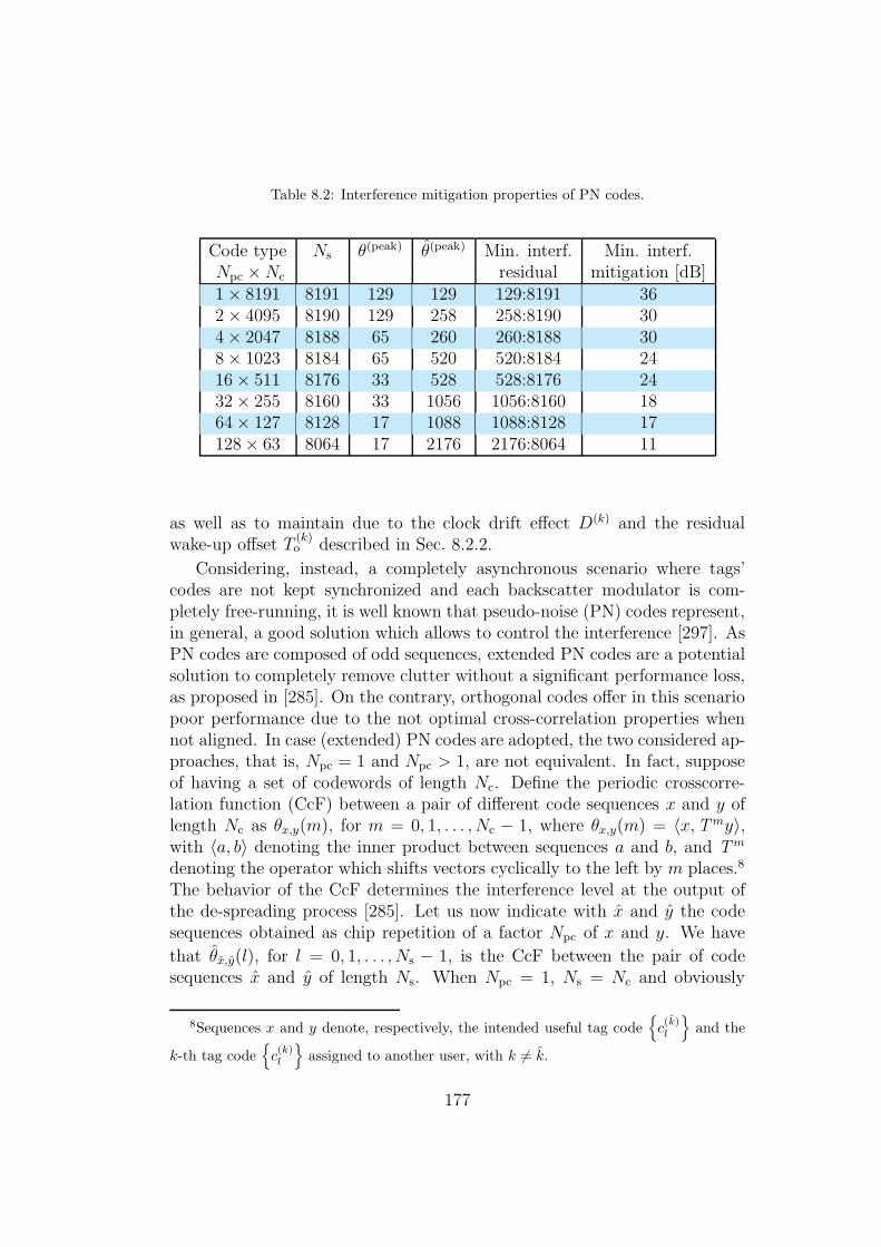
Table 8.2: Interference mitigation properties of PN codes.
Code type Ns θ(peak) θ(peak) Min. interf. Min. interf.Npc ×Nc residual mitigation [dB]1× 8191 8191 129 129 129:8191 362× 4095 8190 129 258 258:8190 304× 2047 8188 65 260 260:8188 308× 1023 8184 65 520 520:8184 2416× 511 8176 33 528 528:8176 2432× 255 8160 33 1056 1056:8160 1864× 127 8128 17 1088 1088:8128 17128× 63 8064 17 2176 2176:8064 11
as well as to maintain due to the clock drift effect D(k) and the residualwake-up offset T
(k)o described in Sec. 8.2.2.
Considering, instead, a completely asynchronous scenario where tags’codes are not kept synchronized and each backscatter modulator is com-pletely free-running, it is well known that pseudo-noise (PN) codes represent,in general, a good solution which allows to control the interference [297]. AsPN codes are composed of odd sequences, extended PN codes are a potentialsolution to completely remove clutter without a significant performance loss,as proposed in [285]. On the contrary, orthogonal codes offer in this scenariopoor performance due to the not optimal cross-correlation properties whennot aligned. In case (extended) PN codes are adopted, the two considered ap-proaches, that is, Npc = 1 and Npc > 1, are not equivalent. In fact, supposeof having a set of codewords of length Nc. Define the periodic crosscorre-lation function (CcF) between a pair of different code sequences x and y oflength Nc as θx,y(m), for m = 0, 1, . . . , Nc − 1, where θx,y(m) = 〈x,Tmy〉,with 〈a, b〉 denoting the inner product between sequences a and b, and Tm
denoting the operator which shifts vectors cyclically to the left by m places.8
The behavior of the CcF determines the interference level at the output ofthe de-spreading process [285]. Let us now indicate with x and y the codesequences obtained as chip repetition of a factor Npc of x and y. We have
that θx,y(l), for l = 0, 1, . . . , Ns − 1, is the CcF between the pair of codesequences x and y of length Ns. When Npc = 1, Ns = Nc and obviously
8Sequences x and y denote, respectively, the intended useful tag code{c(k)l
}and the
k-th tag code{c(k)l
}assigned to another user, with k 6= k.
177

θx,y(l) = θx,y(m), since x = x and y = y. Differently, if Npc > 1 is adopted,
the resulting code of length Ns exhibits a CcF θx,y(l) which can be expressedas a function of the original θx,y(m) as9
θx,y(l) =Npc θx,y(⌊l/Npc⌋) + (l mod Npc) [θx,y(⌊l/Npc⌋+1)− θx,y(⌊l/Npc⌋)] .(8.9)
As it is possible to observe from (8.9), when adopting Npc > 1, the CcF
peak θ(peak) = maxl
{∣∣∣θx,y(l)∣∣∣}, given by θ(peak) = Npcmax
l{|θx,y(⌊l/Npc⌋)|},
is worsen of a factor Npc with respect to the original code, that is θ(peak) =Npc max
m{|θx,y(m)|} = Npcθ
(peak). Thus, the adoption of a code with Npc>1
results in an increasing of the peak (and average) value of the CcF θ(l),that is a decreasing of the code interference mitigation capability. However,it is well known that a shorter sequence presents a lower peak for its CcFθx,y(m), which is directly related to the sequence length [297]. Thus, we havetwo conflicting factors: on one side, the interference level is increased by thefact that Npc > 1, but on the other side it is decreased thanks to the adoptionof a shorter code Nc < Ns.
Table 8.2 shows the values of the peak CcFs θ(peak) and θ(peak) for differ-ent Npc, as well as the resulting minimum interference mitigation level forclassical PN codes, in particular codes derived from maximal connected setsof m-sequences presenting the optimal three-valued cross correlation spec-trum10
{−1,−θ(peak), θ(peak) − 2
}(e.g., Gold sequences) [297].11 Looking at
the last column on the right of Table 8.2 it is evident how the gain in interfer-ence mitigation capability presented by the adoption of a code with shorterNc is not sufficient to counteract the decreasing in interference mitigationcapability due to the increased Npc necessary for guaranteeing the target Ns.Due to this effect, considering an asynchronous scenario, we have that thebest performance in terms of interference mitigation is achieved by adoptingthe strategy with Npc = 1.
Wake-up offset and clock drift constraints Due to the non-idealities ofthe wake-up process described in Sec. 8.2.2, small residual offsets with respectto the reader timing of tag codes are present (quasi-synchronous scenario).In this case it is important to exploit this peculiarity, by assigning (to tags)
9The expression is derived from [297, eq. 1.11].10For Nc = 4095 and Nc = 255 there are no preferred pairs of m-sequences so the
corresponding CcFs do not exhibit the optimal three-valued spectrum.11Similar considerations can be formulated for extended PN codes considering a less
favorable interference mitigation capability.
178

codes able to guarantee the orthogonality (or very small cross-correlationvalues) even in the presence of these small offsets [298]. In the presenceof significant clock drift, the scenario from quasi-synchronous can becomeasynchronous, so that codes are also required to preserve good correlationproperties also in asynchronous conditions.
Moreover a code presenting Npc > 1 is intrinsically more robust to syn-chronization errors and the presence of clock drift. As an example, considerthe useful tag code is shifted of q PRPs with respect to the code generatorat reader side due to the presence of offsets. Thus, the process gain, insteadof being Ns, as expected, is equal to the code autocorrelation function (AcF)
evaluated in q, that is θx,x(q), where x is the tag code{c(k)l
}[285]. Accord-
ing to (8.9), as Npc increases, the AcF function presents smoother transitionsmaking the de-spreading more robust to synchronization errors.
To counteract the effects of the wake-up offset and of clock drift we mayoperate in two directions. The first and simplest solution is to adoptNpc ≫ 1,which guarantees a lower receiver complexity at the expense of a reducednumber of available codewords and lower interference mitigation. This cor-responds to set n = Nspan = 1 and thus (n+ν)∆ = 0 in (8.4). The second andmore complex approach, which uses smaller values of Npc (ideally Npc = 1for the best interference mitigation), requires the adoption of tag code acqui-sition schemes at the receiver to deal with the non ideal wake-up offset, aswell as code tracking schemes to compensate the clock drift. In this case theadoption of a code with good AcF (ideally, m-sequence) is beneficial for ac-quisition and tracking. It has to be remarked that with small Npc it becomesimportant to adopt a small span step ∆ (e.g., ∆ = 1 if Npc = 1) to have arefined code acquisition search which can increase the complexity in case ofhigh wake-up offset T
(k)o . As will be investigated in the numerical results, a
trade-off between Npc, hence the required ∆, and the corresponding systemcomplexity has to be found.
8.4 Tag Detection
8.4.1 Tag Detection Scheme
The first task to be accomplished by the reader is the tag detection, that isthe process to detect the presence of a specific tag in the monitored area.The detection in parallel of N tags requires that N detection circuits are em-ployed at receiver section, with a consequent increase of complexity. For thisreason, the tag detection scheme we propose is a partially non-coherent ap-proach based on energy detection, which helps to keep the system complexity
179

affordable, thanks to the possibility of adopting sub-Nyquist sampling rates[60].
According to the considerations made in Sec. 8.3, we assume to adoptbalanced codes, so that (8.6) reduces to
xn(t) =
Ns−1∑
l=0
dl c(1)l+(n+ν)∆ ru(t−lTp) . (8.10)
The term xn(t) can be further detailed considering that ru(t) is the combi-nation of Ntag tags CRs (backscatter), that is
xn(t) =Ns−1∑
l=0
dl c(1)l+(n+ν)∆
Ntag∑
k=1
ω(k)(t−lTp) (8.11)
where the single-tag channel response is
ω(k)(t) =[(sreader(t)⊗ h(k)(t)
)·m(k)(t)
]⊗ h(k)(t)⊗ hZF(t) . (8.12)
The de-spreading process is then followed by energy evaluations per-formed over the PRP Tp, that is
en,m=
∫ mTED
(m−1) TED
y2n(t) dt n = 1, 2, . . . , Nspan, m = 1, 2, . . . , Nbin (8.13)
with Nbin = ⌊Tp/TED⌋ representing the number of integration bins each PRPis divided into, and with TED the integration time. The detection strategyconsists of comparing each element en,m with a threshold ξn,m. If the energyvalue of at least one bin is above the threshold, then the tag is considereddetected. Obviously, the challenging issues is the evaluation of the thresholdξn,m.
To this purpose, we define the global probability of false alarm (PFA) asthe probability of deciding that the tag is present when it is not present inthe considered environment, and the global probability of detection (PD) theprobability of taking the correct decision when the tag is present. We thendefine H1 and H0 the hypotheses related to the presence and absence of thetag, respectively. The choice of the threshold affects the performance of thedetection scheme in terms of PD and PFA. Low values for the threshold leadto higher PFA and higher PD. The vice versa holds for high values of ξn,m.For further convenience we define the single-bin PFA as the probability thatthe single bin energy exceeds the threshold when the tag is not present, andthe single-bin PD as the probability that the single bin exceeds the thresh-old when the tag is effectively present. Global PFA and PD are indicated
180

0 20 40 60 80 100 1200
10
20
30
40
50
60
Bin Index
Nsp
an
0
1
2
3
4
5
6x 10
−14
Useful Tag
Near−far interference
Figure 8.2: Example of energy matrix E in presence of wake-up offset, clock drift andnear-far interference effect.
in the following with capital letters, specifically PFA and PD, respectively,the single-bin PFA and PD, for the bin of coordinate (n,m), are indicated
with lower cases, specifically p(n,m)FA and p
(n,m)D , respectively. If the threshold
is exceeded, the coordinates (n, m) associated to the maximum provide anestimate of the tag clock offset and a coarse estimate of the signal TOA,respectively, thanks to the adoption of UWB signals. The maximum reso-lution in TOA estimation (and hence ranging) is determined by TED [51].TOA estimates can be further improved by adopting ranging strategies asdescribed in [51].
8.4.2 Threshold Evaluation Criteria
The usual strategy for signal detection is defining a fixed threshold, that isa threshold ξn,m = ξ [111]. However, this approach is not suitable in UWB-RFID systems based on backscatter modulation in presence of multi-tag in-terference. In fact, the useful tag can be hidden by interference peaks comingfrom tags closer to the reader than the intended useful one (i.e., a near-fareffect). This fact is clearly depicted in Fig. 8.2, which shows an example ofenergy matrix E = {en,m} where the near-far effect is evident. If a constantthreshold over all bins were adopted, the PFA would increase significantlydue to the presence of interferers close to the reader. The effect is very pro-nounced in this kind of system due to the two-hop propagation channel, asthe received power, in free-space propagation, is proportional to d4, where d is
181
the reader-tag distance [50, 283]. Assuming a useful and an interferer tag atdistance, respectively, dU and dI from the reader, the difference in the receiv-ing power at reader side from the two tags is 40[log10(dU)− log10(dI)] dB. Forexample, considering a useful and an interferer tag placed, respectively, atdU = 10m and dI = 2m from the reader, we find a difference of approximately27 dB in the signals amplitude. If this difference is not properly managed bythe interference mitigation capability provided by the tag codes, a high PFAdue to near-far effects is expected.12 Unfortunately classical power controlapproaches, as usually adopted in CDMA systems, cannot be used due to thepassive nature of the communication here considered. Therefore we proposea bin-dependent threshold strategy able to counteract near-far effects. In thefollowing the threshold will be analytically computed considering a constanttarget PFA P ∗
FA, under the hypothesis of absence and presence of multi-taginterference.
Consider now the elements en,m of the energy matrix. The presenteddecision rule consist in
Decide :
{H0 , if en,m < ξn,m ∀n,m ,
H1 , if ∃ {n,m} s.t. en,m ≥ ξn,m .(8.14)
Define now the normalized test
Λ(n,m) =2
NsN0
en,mH1
≷H0
ξn,m (8.15)
where ξn,m = 2NsN0
ξn,m. According to the approach proposed in [86] we have
Λ(n,m) =2
NsN0
∫ mTED
(m−1) TED
y2n(t) dt ≃1
σ2
mN∑
i=(m−1)N
y2n,i(t) (8.16)
where N = 2WTED, σ2 = NsN0W is the noise variance, and yn,i are for odd
i (even i) the samples of the real (imaginary) part of the ELP yn(t) of yn(t),with yn(t) = ℜ
{yn(t)e
j2πfct}, taken at Nyquist rate W/2 in each interval
TED.13
It is well known that the output of the energy detector is distributed ac-cording to a central Chi-square distribution, with p.d.f. fC(y, ν), under H0,and according to a non-central Chi-square distribution, with p.d.f. fNC(y, λ, ν),under H1 [86]. For further convenience we report the p.d.f.s of these r.v.s,
12The effects are obviously even more pronounced in presence of multiple interferingtags and multipath propagation.
13We consider WTED ∈ N.
182

having indicated with ν the number of degrees of freedom, and with λ thenon-centrality parameter, that is
fNC(y, λ, ν) =1
2e−
y+λ2
(yλ
)ν−24I ν
2−1(√
yλ) , y ≥ 0, (8.17)
fC(y, ν) =y(
ν2−1)
2ν2Γ(ν2
) e−y2 , y≥0 (8.18)
where Iκ(·) denotes the κth order modified Bessel function of the first kind[106, p. 374] and Γ(·) is the gamma function [106, p. 255].
In the following we propose two different threshold criteria according tothe presence or not of multiple tags in the environment.
Single-Tag Scenario
In the absence of interference (i.e., Ntag = 1) the only component at thede-spreader output under hypothesis H0 is the noise zn(t) (i.e., xn(t) = 0).A threshold-crossing event in absence of the useful tag, causing a false alarm,happens when the r.v. Λ(n,m)|H0 is above the threshold ξn,m, where we haveindicated with Λ(n,m)|H0 the test (8.15) under the hypothesis H0, that is
Λ(n,m)|H0 =2
NsN0
∫ mTED
(m−1) TED
z2n(t) dt ≃1
σ2
mN∑
i=(m−1)N
z2n,i (8.19)
where zn,i are the sampling expansion coefficients of the ELP zn(t) of zn(t).Since zn,i are statistically independent Gaussian r.v.s with zero mean andunit variance, the r.v. Λ(n,m)|H0 is central Chi-square distributed, with N
degrees of freedom. This results in a single-bin PFA p(n,m)FA given by
p(n,m)FA =
∫ ∞
ξn,m
fC(y,N) dy =Γ(
N2, ξn,m
2
)
Γ(N2
) = Γ
(N
2,ξn,m2
)(8.20)
where we used [111, 62] to solve the integral, and with Γ(a, x) =∫∞x
xα−1e−xdx
the upper incomplete gamma function and Γ(·, ·) the gamma regularized func-tion. Since the only component at the de-spreader output is the noise zn(t),
the single-bin PFA results to be the same in each bin, that is p(n,m)FA = pFA,
∀n,m. This leads to a constant threshold ξn,m = ξ, ∀n,m. Under the as-sumption of independent energy bins in n and m we have that the global
183
PFA is14
PFA = 1− (1− pFA)M ≃ MpFA (8.21)
where M = Nbin ×Nspan. The threshold ξ, corresponding to the global PFAP ∗FA, can be then calculated by inverting (8.21) and (8.20) obtaining
ξ =NsN0
2· 2 Γ−1
(P ∗FA
M,N
2
)(8.22)
which now depends on the target PFA P ∗FA.
Once the threshold is set to guarantee a certain PFA, we can determinethe correspondent single-bin PD. Under the hypothesis H1, the ED statisticsΛ(n,m)|H1 is given by
Λ(n,m)|H1 =2
NsN0
∫ mTED
(m−1) TED
(xn(t) + zn(t))2 dt ≃ 1
σ2
mN∑
i=(m−1)N
(xn,i + zn,i)2
(8.23)where xn,i are the sampling expansion coefficients of the ELP xn(t) of x(t).Since zn,i are statistically independent Gaussian r.v.s with zero mean andunit variance, the r.v. Λ(n,m)|H1 is non-central Chi-square distributed, withN degrees of freedom, and non-centrality parameter λn,m = 2γn,m, where theSNR per bin is denoted by
γn,m =1
NsN0
∫ mTED
(m−1) TED
xn(t)2 dt ≃ 1
2σ2
mN∑
i=(m−1)N
x2n,i . (8.24)
The single-bin PD p(n,m)D is then given by [111, 62]
p(n,m)D = Qk
(√λn,m,
√ξ
)(8.25)
where k = N/2 and Qk(α, β) =∫∞β
x ( xα)k−1 exp
{−x2+α2
2
}Ik−1(αx) dx is the
generalized Marcum’s Q function of order k. The global PD PD can be finallycomputed as
PD = 1−Nspan∏
n=1
Nbin∏
m=1
(1− p
(n,m)D
)(8.26)
under the assumption of having independent energy bins.
14This assumption is exact in case of Nspan = 1, since the energy bins are independent,while results an approximation when Nspan > 1 as the energy matrix elements are corre-lated for different code shifts. Consequently, (8.22) leads to a threshold more conservativethan the necessary and, consequently, a PD lower than expected.
184

Multi-Tags Scenario
We now extend the derivation 8.4.2 to include the multi-tag interferenceeffect in the threshold evaluation process. As previously discussed, a properthreshold design is fundamental to avoid the detrimental effects of near-farinterference.
We consider now Ntag tags placed in the environment. Without loss of
generality we consider tag k = 1 as the intended one to be detected, whiletags for k = 2, 3, . . . , Ntag are considered as interferers. In this case, alsoin absence of the useful tag, xn(t) 6= 0 due to the presence of the residualinterference term after the de-spreading [285]. For further convenience, wedistinguish the case whether the desired tag is present or absent, by defining
{x(H0)n (t) =
∑Ns−1l=0 dl c
(1)l+(n+ν)∆
∑Ntag
k=2 ωk(t) ,
x(H1)n (t) =
∑Ns−1l=0 dl c
(1)l+(n+ν)∆
∑Ntag
k=1 ωk(t) .(8.27)
Since zn,i are statistically independent Gaussian r.v.s with zero mean andunit variance, under both hypotheses H0 and H1 the r.v. Λ, that is, theED output, is non-central Chi-square distributed with N degrees of freedom,and with a non-centrality parameter depending on H0 and H1. Under thehypothesis H0 (no useful tag), the ED output results in
Λ(n,m)|H0 =2
NsN0
∫ mTED
(m−1)TED
(x(H0)n (t)+zn(t)
)2dt≃ 1
σ2
mN∑
i=(m−1)N
(x(H0)n,i + zn,i
)2
(8.28)
where x(H0)n,i are the sampling expansion coefficients of the ELP x
(H0)n (t) of
x(H0)n (t), leading to the non-centrality parameter λ
(H0)n,m = 2γ
(H0)n,m where the
interference-to-noise ratio (INR) per bin is defined as
γ(H0)n,m =
1
NsN0
∫ mTED
(m−1) TED
x(H0)n (t)2 dt ≃ 1
2σ2
mN∑
i=(m−1)N
(x(H0)n,i
)2. (8.29)
A threshold-crossing event in absence of the useful tag, causing the falsealarm event, happens when the r.v. Λ(n,m)|H0 is above the threshold ξn,m.
This results in a single-bin PFA p(n,m)FA given by
p(n,m)FA =
∫ ∞
ξn,m
fNC(y, λ(H0)n,m , N) dy = Qk
(√λ(H0)n,m ,
√ξn,m
)(8.30)
where we used [111, 62] to solve the integral. The non-centrality parametersare strictly related to the interference level at each bin en,m, then a constant
185

PFA in each bin, that is p(n,m)FA = pFA, ∀n,m, is obtained if a bin-dependent
threshold ξn,m is adopted according to (8.30). In particular, under the as-sumption of independent energy bins in n and m as in (8.21), the thresholdξn,m can be calculated from (8.21) and (8.30) as
ξn,m =NsN0
2·[Q−1
k
(√λ(H0)n,m ,
P ∗FA
M
)]2(8.31)
with Q−1k (·, ·) denoting the inverse generalized Marcum Q function. Again,
once the bin-dependent threshold is set to guarantee a certain PFA, we candetermine the corresponding single-bin PD. Under the hypothesis H1, theED output is described by
Λ(n,m)|H1 =2
NsN0
∫ mTED
(m−1)TED
(x(H1)n (t)+zn(t)
)2dt≃ 1
σ2
mN∑
i=(m−1)N
(x(H1)n,i +zn,i
)2
(8.32)
where x(H1)n,i are the sampling expansion coefficients of the ELP x
(H1)n (t) of
x(H1)n (t), leading to the non-centrality parameter λ
(H1)n,m = 2γ
(H1)n,m , where the
interference-plus-signal-to-noise-ratio (ISNR) per bin is defined as
γ(H1)n,m =
1
NsN0
∫ mTED
(m−1) TED
x(H1)n (t)2 dt ≃ 1
2σ2
mN∑
i=(m−1)N
(x(H1)n,i
)2. (8.33)
The single-bin PD p(n,m)D is then given by [111, 62]
p(n,m)D = Qk
(√λ(H1)n,m ,
√ξn,m
)(8.34)
and the global PD PD can be computed according to (8.26).The presented tag detection scheme in the presence of interference re-
quires the knowledge of the INR per bin in order to define the proper bin-dependent threshold ξn,m according to (8.31) necessary to keep PFA < P ∗
FA.In Sec. 8.5 practical approaches for defining the threshold without exact a-priori knowledge of the interference level will be detailed.
Note that the detection performance in terms of PD in (8.25) and (8.34)is related to Ns. Since the transmitting power of the UWB transmitter isconstrained by maximum spectrum emission masks, Ns results the designparameter to be determined to guarantee a target PD P ∗
D given a certainreader-tag distance. Numerical results in Sec. 8.5 will provide an example ofsystem design.
186

8.5 Numerical Results
In this section we present an example of system design, and performanceevaluated in realistic conditions. Specifically we analyze the tag detectionrate as a function of the false alarm rate considering the low complexitynon-coherent scheme based on energy detection proposed in Sec. 8.4.
8.5.1 Simulation Parameters
We assume to perform the tag detection in a preamble consisting of data
symbols{b(k)m
}of all ’+1’. We considered a scenario with a system composed
of one reader, and one or more tags placed in the direction of reader’s antennamaximum radiation. In addition, we considered the signal backscattered byany untagged object as part of the clutter.
We adopt Tp = 128 ns.15 A reader with Gr = 5dBi antenna gain, tagsequipped with an Gr = 1dBi antenna and Lt = 2dB switch losses havebeen considered. Results have been obtained starting from multipath chan-nel responses with exponential power delay profile and Nakagami-m fading(severity factor m=3), a rms channel delay-spread of 10 ns16 and paths sepa-rated of 2 ns apart. A transmitted signal compliant with the IEEE 802.15.4aemission mask in the 3−5GHz is considered, adopting RRC pulses17 withpulse width parameter Tw = 1ns, roll-off factor ν = 0.6 and center frequencyfc = 4GHz. For what concerns the clutter, a worst-case of uniform powerdelay profile in the overall interval Tp is considered, with paths spaced 0.95 nsapart, each path with amplitude characterized by Nakagami-m fading, withm = 3, and a rms value of 0.5mV at the receiver. In addition, at receiverside a figure noise F = 4dB is considered and an ideal bandpass filter band-width W = 2GHz and center frequency fc = 4GHz. Energy evaluations areperformed with a bin of width TED = 1ns.
8.5.2 System Design
Link budget and system parameter choice
The principal parameter to be accounted in the system design is the numberof pulses per symbol Ns, in order to guarantee a target PD P ∗
D at a certain
15This and the next system specifications are driven by the outcome of the Europeanproject SELECT, http://www.selectwireless.eu
16This value is comprehensive of the two-way link of the backscatter signal [283].17See (3.63) for the definition.
187

maximum reader-tag distance, which poses a constraint on a minimum Ns.Thus, the relation Ns ≥ Ns has to be satisfied.
This parameter can be easily derived under some approximations. Inparticular we assume i) AWGN conditions, ii) that the received pulse alwaysfalls entirely in one bin, iii) absence of interference and ideal tag code phaseretrieving with Nspan = 1. In this case the single-bin detection probability
p(n,m)D equals the system detection probability PD, which will be imposedequal to the target P ∗
D. Specifically, according to (8.25), we have
P ∗D = Qk
(√λ(d),
√ξ
)(8.35)
with λ(d) = 2 SNRp(d), having indicated with SNRp(d) the SNR obtained inAWGN and free-space conditions after the de-spreading process for a reader-tag distance d, that is
SNRp(d) =Ns
N0
Ep
PL(d). (8.36)
The factor PL(d) indicates the free-space pathloss, that is18
PL(d) =
(4π d fc
c
)4Lt
G2r G
2t
(8.37)
with c denoting the speed of light. Noticing that ξ, given by
ξ = 2 Γ−1
(P ∗FA
Nbin,WTED
)(8.38)
is not function of Ns, it is possible to obtain the number of pulses per symbolinverting (8.35) as
Ns ≥⌈N0PL(d)
2Ep
[Q−1
k
(P ∗D,
√ξ
)]2⌉(8.39)
with Q−1K (·, ·) denoting the inverse generalized Marcum Q function, N0 =
kB F To, To = 290K the reference temperature, and kB the Boltzmann con-stant. Substituting the simulation parameters indicated in Sec. 8.5.1, andconsidering P ∗
FA = 10−3 and P ∗D = 0.9, we obtain the curve providing Ns as
function of the distance depicted in Fig. 8.3. For comparison, in the samefigure, results obtained considering a transmitting power exceeding the FCC
18Here we adopt a central-frequency approximation. The reader gain Gr is only ac-counted once since the transmitted energy Ep already accounts for it at transmitting side.
188

0 1 2 3 4 5 6 7 8 9 10 11 12 13 1410
0
101
102
103
104
105
d [m]
Ns
Energy Detection (FCC+10dB)Coherent Demodulation (FCC+10dB)Energy Detection (FCC)Coherent Demodulation (FCC)
Figure 8.3: Minimum number of pulses per symbol as function of the reader-tag distance.
mask of 10 dB is also reported, as well as the resulting Ns coming from adifferent analysis, specifically from the fulfillment of a requirement of BEPPeb higher of a target P ∗
eb = 10−3. Considering an ideal MF and AWGNconditions this can be derived from19
Ns ≥N0PL(d)
Ep
erfc−1 (2P ∗eb)
2 . (8.40)
It is possible to notice how the number of minimum pulses per symbol issignificantly higher for the receiver here considered. This is mainly due tothe fact that the detection process is non-coherent. Moreover, consideringthat it is important to keep the symbol time not too high in order to ensurea channel static (for clutter removal) and the phase noise constant on asymbol (for clock drift problems), practical values of Ns are around 10000.This corresponds to a detection range between 6 and 7 so not satisfactoryfore some applications. In this case it can be noticed how an increasing ofthe transmitting power is high effective for reducing the number of pulsesneeded.20 Differently, it is necessary to adopts more sophisticated receivers,
19Note that the presented architecture does not allow coherent bit demodulation sinceit is energy-based. However, sub-optimal hybrid solutions, as for example presented in[299], allow taking advantage of the low-complexity receiver structure here described alsoallowing bit demodulation provided that symbols are differentially encoded (i.e., withdifferential binary phase shift keying (DBPSK) modulation at tag side).
20Moreover it is possible to adopt antennas with higher gain, but in this case the effective
189
able to collect the energy from the environmental multipath, and combineit for detection and demodulation purposes. In the following performanceanalysis we adopt Ns = 8192, corresponding to a symbol time Ts ≈ 1ms.
Tag Code Assignment
For what concerns the code family choice, an interesting possibility for theUWB-RFID system is to adopt Orthogonal Gold codes [300]. These codesare exactly orthogonal in the synchronous scenario (l = 0) and maintainthe properties of extended Gold Codes (low cross-correlation) in the asyn-chronous scenario. They are constructed by lengthening of one chip thePreferentially-Phased Gold codes [301], that present the optimum value −1of cross-correlation between all the pairs of codewords when aligned. In thismanner an even code is obtained enabling the complete clutter cancellation.By using these codewords, the detection procedure is performed in a quasi-orthogonal environment without suffer of interference. The possibility ofadopting such a family of codes is very interesting in presence of wake-upoffset and possibility of avoiding code acquisition by increasing Npc: sincethe codes present an orthogonal behavior when aligned, increasing Npc doesnot causes excessive interference degradation during the detection phase.
8.5.3 Results in Multi-Tags Scenario
In Fig. 8.4, we report the receiver operating characteristic (ROC) correspond-ing to perfectly synchronous and asynchronous scenarios with ideal codephase retrieving, related to a useful tag placed at 7m from the reader. Weconsider 59 interfering tags uniformly distributed in two meters around theuseful tag, to reproduce interference effects. In particular, orthogonal Walshcodes in synchronous scenario represent the benchmark, since the interfer-ence is completely removed. On the contrary, their performance drasticallydegrades when the scenario becomes asynchronous. For what extended Goldcodes are concerned, obtained by lengthening of one chip the Gold codeswithout any kind of phase optimization when aligned, they evidence a losswhile the scenario is synchronous, but they allow satisfactory detection ca-pabilities also in asynchronous conditions. Orthogonal Gold codes representinstead the best trade-off for both scenarios since they achieve a detectionrate higher than 0.8 with a false alarm of 10−3 also in the asynchronous sce-nario, while maintaining the optimal behavior of Walsh codes in perfectly
improvement is given by the antenna gain at receiver side only, since the regulations areimposed on the EIRP. This means that the adoption of a higher gain at transmitting siderequires a decrease of the transmitting power of the same amount.
190

10−3
10−2
10−1
100
0.7
0.75
0.8
0.85
0.9
0.95
1
False Alarm Rate
Det
ectio
n R
ate
Orthogonal Walsh−Hadamard
Orthogonal Gold
Extended Gold
Figure 8.4: ROC for the tag detection in UWB backscatter system. Continuous lines (–)refer to the perfectly synchronous scenario, dashed lines (- -) refer to the asynchronousscenario due the presence of clock drift, with ideal code phase retrieving.
synchronous scenario.
It should be remarked that in this simulation near-far effects are negligi-ble, as all the users were approximately placed at the same distance from thereader. To understand this problem, Fig. 8.5 shows the ROC when the usefultag is placed at 6m from the reader, and 19 interfering tags are uniformlydistributed between 2.8m and 3.2m. Orthogonal Gold codes are adopted, asynchronization offset of 500 ns, and a drift of 100 ppm are considered. The16th bit of the transmitted preamble (a sequence of all ’+1’) is analyzed fordetection purposes and the acquisition window is fixed to 40Tp when per-forming synchronization. As clearly depicted in Fig. 8.5, the system suffersfrom near-far effects when a constant threshold over all the bins is considered(dashed lines). Thus a possible solution is represented by the adoption of athreshold which accounts for the interference effects, that is, a bin-dependentvariable threshold computed such that, in the presence of interference, thePFA is constant for each bin. An empirical approach adopted for simulationsconsiders a threshold reflecting the tag pathloss behavior until the tag en-ergy, evaluated in TED, falls below the noise floor N0WTED, then fixing thethreshold to a constant value for the last bins. Figure 8.5 shows that, whenthe bin-dependent threshold is adopted (continuous lines), near-far effectsare significantly mitigated and a detection rate higher than 0.8 with a false
191

10−3
10−2
10−1
100
0.7
0.75
0.8
0.85
0.9
0.95
1
False Alarm Rate
Det
ectio
n R
ate
Nspan = 1, ∆ = 1 (no synchronization)
Nspan = 11, ∆ = 4
Nspan = 41, ∆ = 1
No drift
Constant threshold
Bin−dependent threshold
Figure 8.5: ROC for tag detection in presence of synchronization offset, clock drift andnear-far interference effects. Continuous lines (–) refer to the bin-dependent threshold,dashed lines (- -) refer to the constant threshold.
alarm of 10−3 can be achieved when Nspan is set to 41 to counteract the clockoffset. Vice-versa, adopting Nspan = 11, a lower detection rate is obtainedsince the synchronization scheme is less robust for the considered Nc=1024.Fixing Nspan=1, that is, without code acquisition, no detection capabilitiescan be assured even when a bin-dependent threshold is chosen. Further re-sults assessing the performance of the proposed bin-dependent threshold andcomparing the effects of different code assignment strategies will be includedin a following up publication [37].
8.6 Implementation Issues
We know report several implementation issues to be addressed for the practi-cal realization of the system, as well as solutions to cope with these problemsand impairments.
8.6.1 Receiver Dynamic Range
In practical implementation it is important to ensure a correct level of thereceived signal (both useful and interfering) in order to reduce the possibilityof analog-to-digital converter (ADC) saturation or under quantization. For
192
this reason it is important to analyze the characteristics of the signal expectedat the reader receiving antenna. The overall signal present at the input of aspecific reader is composed of different components:
• The signals backscattered by the tags related to the interrogation ofthe specific reader itself;
• The signals backscattered by the tags related to the interrogation signalof other readers (i.e., an interference component);
• Other readers direct interference, that is, the ensemble of signals emit-ted by other readers;
• The clutter, that is the signal emitted by the specific reader and re-flected by the environment.
These components must be carefully considered, in order to define the dy-namic range at the reader input port and possible issues related to it. For thesake of a complete characterization of the dynamic range, it is important tocomprehend if the strongest received signal comes from an interfering reader,or it comes from the reflections of the environment, as well as the ratio be-tween the strongest input signal and the tag backscattered signal (which issupposed to be strongly attenuated from the backscattering two-way chan-nel).
The pathloss related to the different received signals, obtained adoptingthe free-space propagation model at a single central frequency, can be writtenas
PLr−t =PT
P tR
=
[G2
rG2t
(λ
4πdr−t
)4]−1
, (8.41)
PLr−r =PT
P rR
=
[G2
r
(λ
4πdr−r
)2]−1
, (8.42)
PLr−obj =PT
P objR
=
[σG2
r
λ2
(4π)3
(1
dr−t
)4]−1
(8.43)
where PT is the transmitted power, P tR, P
rR and P obj
R are the received powersfrom tag, reader and objects, respectively, Gr the reader antenna gain, Gt thetag antenna gain, λ is the wavelength, dr−t is the reader-tag distance, dr−r
193

is the reader-reader distance.21 The first term PLr−t accounts for the usefulreader-tag-reader backscattering information signal, that is the useful signalcomponent of interest for detection, TOA estimation and packet demodu-lation. The second term, PLr−r accounts for the direct path coming froman interfering reader: for a localization system we have in fact to deploy anetwork composed of at least three readers in order to perform trilaterationonce estimated the reader-tag distances. The last term PLr−obj accounts forone of the clutter components, due to the reflection on a scatter with a radarcross section (RCS) σ (e.g., the object to which the tag is attached). In factit is supposed that each tag is attached to a bigger object whose reflectionproperties, characterized by its RCS, could determine the presence of a strongclutter component having the same TOA of the useful signal. In particular,equations (8.41) and (8.43), that represent respectively the pathloss for tagand object backscattering, derive from the well known radar range equation.On the contrary, equation (8.42), that is the interfering signal coming froman other reader, is derived from the well known Friis formula.
0 2 4 6 8 10 12 1410
−8
10−7
10−6
10−5
10−4
10−3
10−2
10−1
Reader−Tag distance [m]
Am
plitu
de [V
]
Backscatter Peak Signal AmplitudeClutter Peak AmplitudeInterference Peak Amplitude − 5x5 cellInterference Peak Amplitude − 7x7 cellInterference Peak Amplitude − 10x10 cell
Figure 8.6: Typical dynamic range of a UWB-RFID system.
In Fig. 8.6, the peak of the received signals are reported considering threedifferent reader-reader distances (i.e., three different square cell sizes), an ob-ject to which the tag is attached presenting the worst case RCS of a square
21For UWB signals all the terms should be characterized as function of the frequency.This is a central-frequency approximation useful for understanding the signal level at thereceiver side.
194

metallic plate of 50 × 50 cm.22 The figure illustrates how the maximum re-ceived signal is usually the one coming from the opposite reader, dependingon the cell dimensions. This means that the strongest signal at the reader in-put port is, in many situations, determined by the direct interference comingfrom the opposite reader.
8.6.2 Multi-Reader Interference
As already described, in the UWB-RFID network several readers (e.g., fouras in the square cell scenario we are considering) are in charge of monitoringa determined area. It is clear how, in this manner, it is necessary to enablethe possibility of accessing the same tag by multiple readers, with a potentialproblem of inter-reader interference.
For this analysis we consider the square scenario reported in Fig. 6.2with the four readers placed at the corners of the cell. We now neglect thepresence of obstacles, assuming that the greatest interference comes from theopposite reader in case of free-space propagation.23 Focusing, whitout loss ofgenerality, on the interference generated by Reader 3 (opposite Reader) andreceived by Reader 1, we can thus foresee three different situations:
1. The interfering signal is reflected (backscattered) by the useful tag (i.e.,the tag which Reader 1 wants to detect or demodulate);
2. The direct path (or the multipath) between Reader 3 and Reader 1(i.e., the already analyzed strongest interfering signal) exists;
3. The interfering signal is reflected by a tag different from the useful one.
We assume that the interrogation signals transmitted by Reader 3 and
Reader 1 are generated adopting, respectively, the spreading codes{d(3)i
}
and{d(1)i
}, and that that the useful and the interfering tags have codes
{c(u)i
}and
{c(int)i
}, respectively. To detect the presence of the useful tag,
Reader 1 performs a de-spreading using the composed code{d(1)i · c(u)i
}, ac-
cording to the procedure that described in detail in Chapter 7 and Sec. 8.4.
22Typical system parameters for antennas are accounted in the derivation. See, for adescription, Sec. 8.5.1.
23In general we can assume a lower level for the interference of the two neighbor readersin the case of partial directive antennas at transmitting and/or receiving stage, while ahigher level for the interference coming from the two neighbor readers in case of adoptionof omnidirectional antennas.
195
As anticipated, the direct link between Reader 3 and Reader 1 representsthe strongest interfering signal. Considering, in fact, the intended useful tagplaced, for example, at the center of the square cell at distance d = 7m fromthe Reader 1, we have that the received tag backscatter signal scales with d4,while the interfering Reader 3 direct signal scales with (2d)2. It is immediatefrom free-space propagation equations (8.41) and (8.42) that the differencein the received power (in dB) between the interfering reader and the usefultag is given by
20 log (d)− 20 log
(c
2πfc
)(8.44)
where c denotes the speed of light and fc the signal central frequency, andwhere we have adopted, for simplicity, a unitary tag antenna gain. Substi-tuting the value d = 7m we obtain a difference between the two receivedpowers of about 55 dB. If a CDMA-based technique is adopted for read-ers MAC, even a very small de-spreading residual interference componentcan completely vanish the possibility of detecting and demodulating a tagsignal. Moreover, as seen in Sec. 8.3, readers’ code has to fulfill several re-quirements. In particular, relating to the previously presented three cases,the multi-reader interference is cancelled provided that the following threeconditions are satisfied:
1. Cancellation of the multi-reader interference component modulated bythe useful tag:
Ns∑
i=1
d(1)i c
(u)i d
(3)i c
(u)i =
Ns∑
i=1
d(1)i d
(3)i = 0 (8.45)
2. Cancellation of the direct reader-reader interference:Ns∑
i=1
d(1)i d
(3)i c
(u)i = 0 (8.46)
3. Cancellation of the multi-reader interference component modulated byan other tag:
Ns∑
i=1
d(1)i c
(u)i d
(3)i c
(int)i = 0 (8.47)
These stringent requirements24 pose several challenges on readers’ codes de-sign, especially for the almost-ideal interference cancellation capability re-quired. Moreover, the cancellation can be obtained by suitable orthogonal
24For example, the requirement 3 must be fulfill for all the possible tag sequences sinceit is necessary to remove the interference due to all the possible tags.
196

codes, but this fact poses further constraints on the synchronization levelthat the readers network has to provide.25
For this reason it is clear how a CDMA-based readers MAC scheme iscritical, and simpler solutions, such as TDMA, have to be accounted atreader side, especially for low-complexity realizations. Specifically, it consistsof alternating in a cyclic way the transmitting reader, with the other readersin receiving mode. Adopting TDMA the interference problem coming fromother readers is completely avoided.
TDMA can be performed at different rates considering the alternationof the transmitting reader, for example, each symbol or each packet. De-creasing the switching rate between readers (e.g., implementing TDMA atpacket level) allows preventing problems deriving from synchronization mis-matches, whereas the main drawback is the reduction of the update rate andconstraints on the maximum tags’ allowed speed, when object tracking isperformed.
It is worthwhile to highlight that even the MAC at reader level wereTDMA-based, the access from each reader to multiple tags would be stillCDMA-based.
8.6.3 Analog-to-Digital Conversion
The main reader functionality is to perform the signal de-spreading in orderto detect and demodulate the tag signal, and to ensure the clutter cancella-tion. In principle this process can be performed in the analog or digital do-main, as well as pre or post a matched filtering operation. If the de-spreadingis realized in analog (both pre or post matched filtering and sampling), theoutput signal to be digital converted consists simply of the useful tag con-tribution and interference residual, as seen in Chapter 7 and Chapter 8. Inthis case the ADC dynamic can be adjusted on the maximum tag expectedsignal, considering, for example, a tag as close as much allowed to the reader.
Notice that, when a synchronization scheme is adopted exploiting the di-rect reader-to-reader UWB signals, or a multistatic WSR capability has tobe guarantee, it is necessary to ensure that the interfering reader signal doesnot saturate the low-noise amplifier (LNA) at receiver side, also if TDMAis adopted as readers MAC. In this case a fixed amplifier gain is sufficient,since the signal amplitude is fixed once the cell size is defined. Vice versa, ifreaders’ synchronization is not performed exploiting the UWB transceivers,multistatic techniques are not adopted, and TDMA is adopted as readersMAC, the input LNA can be designed in order to prevent saturation due to
25See Sec. 6.3.2.
197
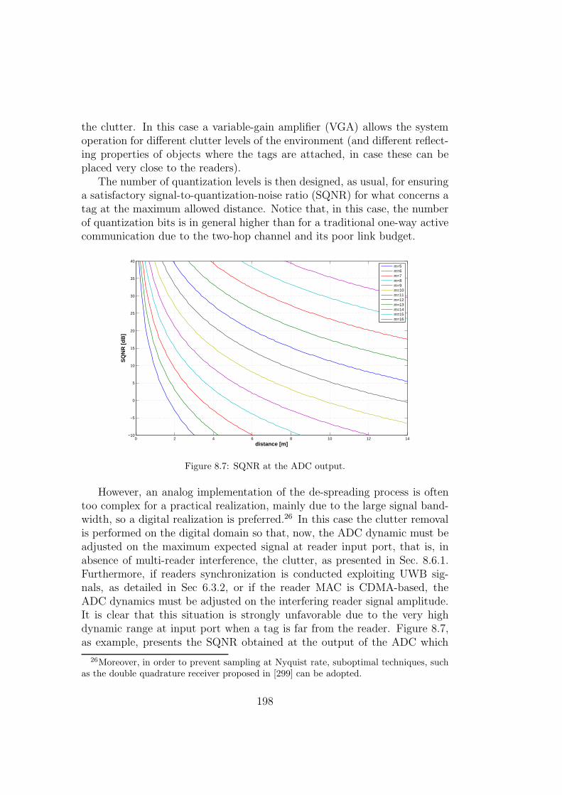
the clutter. In this case a variable-gain amplifier (VGA) allows the systemoperation for different clutter levels of the environment (and different reflect-ing properties of objects where the tags are attached, in case these can beplaced very close to the readers).
The number of quantization levels is then designed, as usual, for ensuringa satisfactory signal-to-quantization-noise ratio (SQNR) for what concerns atag at the maximum allowed distance. Notice that, in this case, the numberof quantization bits is in general higher than for a traditional one-way activecommunication due to the two-hop channel and its poor link budget.
0 2 4 6 8 10 12 14−10
−5
0
5
10
15
20
25
30
35
40
distance [m]
SQ
NR
[dB
]
m=5m=6m=7m=8m=9m=10m=11m=12m=13m=14m=15m=16
Figure 8.7: SQNR at the ADC output.
However, an analog implementation of the de-spreading process is oftentoo complex for a practical realization, mainly due to the large signal band-width, so a digital realization is preferred.26 In this case the clutter removalis performed on the digital domain so that, now, the ADC dynamic must beadjusted on the maximum expected signal at reader input port, that is, inabsence of multi-reader interference, the clutter, as presented in Sec. 8.6.1.Furthermore, if readers synchronization is conducted exploiting UWB sig-nals, as detailed in Sec 6.3.2, or if the reader MAC is CDMA-based, theADC dynamics must be adjusted on the interfering reader signal amplitude.It is clear that this situation is strongly unfavorable due to the very highdynamic range at input port when a tag is far from the reader. Figure 8.7,as example, presents the SQNR obtained at the output of the ADC which
26Moreover, in order to prevent sampling at Nyquist rate, suboptimal techniques, suchas the double quadrature receiver proposed in [299] can be adopted.
198

maximum dynamic is adjusted on the interfering opposite reader signal on a10 × 10m square cell, as function of the reader-tag distance and for differ-ent number of quantization bits m, with m = log2 (L) and L the number ofquantization levels. It is immediate to observe how, in this case, a very highnumber of bits is necessary in order to provide a satisfactory SQNR, for ex-ample a value so that the quantization noise is negligible with respect to thethermal noise. Fortunately, this requirement can be relaxed, by consideringthe presence of the digital de-spreading process, which can significantly help.
In fact, in Appendix 8.A it is shown that, in presence of low SNR condi-tions, as the case of the UWB-RFID system for the received tag signal, theprocess gain is beneficial not only for increasing the effective SNR but alsofor the SQNR. In particular, if Ns CRs are accumulated at receiver side,both the SNR and the SQNR are enhanced of a factor Ns with respect tothe same quantities at the output of the ADC, prior the de-spreading stage.In this manner it is possible to significantly reduce the target SQNR at theoutput of the ADC, without suffering of quantization noise on the effectivede-spreaded signal. The number of quantization bits can be in this mannersignificantly reduced.
8.7 Conclusion
In this chapter we have presented the UWB-RFID systems based on backscat-ter modulation, in presence of interference, wake-up synchronization offsetand clock drift, considering a practical low-complexity tag detection scheme.Tag detection performance has been evaluated in terms of detection and falsealarm probability, to analyze the robustness of different code families in dif-ferent scenarios. It has been shown that the joint use of orthogonal Goldcodes with proper low-complexity detection and code acquisition schemesinvolving bin-dependent thresholding is a promising solution to overcomeimplementation impairments and near-far effects. Several implementationissues have been analyzed and possible solutions to cope with problems ofdynamic range, A/D conversion and multi reader interference proposed.
8.A Effect of De-Spreading on A/D Conver-
sion
The purpose of this analysis is to derive the relationship between the SQNRat the output of the ADC and of the de-spreader as a function of the numberof pulses Ns. Figure 8.8 shows the analyzed ADC and de-spreader, where
199

Figure 8.8: The considered scheme for the ADC and de-spreader.
the ADC output is multiplied by the tag code, and then it is accumulatedfor Ns times.In particular, we can express the input signal X as:
X = xu + xc + ni (8.48)
where xu is the useful signal component, xc is the clutter/interference compo-nent (which mainly affects the upper bound of the dynamic range at the ADCinput), and ni is the additive thermal noise. The useful signal componentand the clutter component are assumed uniformly distributed respectively in[Xmin, Xmax] and [−Xc,max, Xc,max], but they are considered both constantwithin a symbol time.
We can express X as
X = xu + xc + ni + ǫx (8.49)
where ǫx is the quantization noise error. We assume the quantization noiseuniformly distributed in [0, δ], where δ corresponds to the quantization stepamplitude.27 Now, if we look at the output of the accumulator, we canexpress Y (under the hypothesis of zero mean code) as
Y = Ns · xu + nout + ǫy (8.50)
where nout is given by
nout =Ns∑
i=1
ci · ni (8.51)
and ci represents the i-th chip of the codeword.The SQNRs SQNRin and SQNRout, respectively, at the output of the
ADC and of the accumulator are:
SQNRin =E {x2
u}E {ǫ2x}
(8.52)
27Assuming that a sufficient high number of quantization bits is adopted and that thesum of signal and noise is above the quantization step.
200

and
SQNRout =N2
s · E {x2u}
E{ǫ2y} (8.53)
In the following, we find the relationship between E{ǫ2y}and E {ǫ2x}. In
particular, we can write the second-order moment of ǫy as
E{ǫ2y}= E
(Ns∑
i=1
ci · ǫxi
)2
= E
{Ns∑
i=1
c2i · ǫ2xi+ 2 ·
Ns−1∑
i=1
Ns∑
j=i+1
ci · ǫxi· cj · ǫxj
}(8.54)
We derive now (8.54) for two extreme cases: low SNR (where the thermalnoise amplitude is larger than the quantization step and the useful signalamplitude), and high SNR (thermal noise negligible with respect to the usefulsignal and the quantization step). The first is the condition of interest for theUWB-RFID system, while the second is reported for sake of completeness.
Analysis at low SNR In this case, we can assume that ǫxiand ǫxj
areindependent (due to the Gaussian thermal noise), obtaining:
E
{2 ·
Ns−1∑
i=1
Ns∑
j=i+1
ci · ǫxi· cj · ǫxj
}= 0 (8.55)
and thus we can write
E{ǫ2y}= E
Ns∑
i=1
c2i · ǫ2xi= E
{Ns∑
i=1
c2i · ǫ2xi
}
=
Ns∑
i=1
c2i · E{ǫ2xi
}= Ns · E
{ǫ2x}. (8.56)
Finally we have the expression:
SQNRout =N2
s · E {x2u}
Ns · E {ǫ2x}= Ns · SQNRin (8.57)
where it is evident the processing gain of Ns shown also in Fig. 8.9. In thesame figure, it is evident how five bits are not sufficient for the quantization,and thus there is no gain in the SQNR.
201

0 1000 2000 3000 4000 5000 6000 7000 80000
1000
2000
3000
4000
5000
6000
7000
8000
9000
Ns
SQ
NR
out/S
QN
Rin
5 bits8 bits11 bits14 bits
Figure 8.9: SQNR gain after de-spreading and accumulation.
Analysis at high SNR If we assume to work at high SNR, we can neglectni with respect to xu. Consequently, equation (8.55) is no more valid, sinceǫxi
and ǫxjare not statistically independent (considering one observed bit,
clutter is constant and the useful signal assumes only 2 values). Consideringthat ǫx depends only on the transmitted chip (+1 or -1), we can write (8.54)as:
E{ǫ2y}=E
Ns2∑
i=1
c2i · ǫ2xi|+1 +Ns∑
i=Ns2+1
c2i · ǫ2xi|−1+ (8.58)
+2 ·Ns2−1∑
i=1
Ns2∑
j=i+1
ci · ǫxi|+1 · cj · ǫxi|+1+
+2 ·Ns−1∑
i=Ns2+1
Ns∑
j=i+1
ci · ǫxi|−1 · cj · ǫxi|−1
= E
ǫ2x|+1 ·
Ns2∑
i=1
ci
2
+ ǫ2x|−1 ·
Ns∑
i=Ns2+1
ci
2
where we assumed to have for simplicity a sequence of +1 until Ns
2and of
-1 from
(Ns
2+ 1
)until Ns, and that ǫxi|+1 and ǫxi|−1 depends only on the
202

transmitted chip (it means ǫxi|−1 = ǫx|−1 and ǫxi|+1 = ǫx|+1 for any i-th chip.Then we can write
E{ǫ2y}= E
{(Ns
2· ǫx|+1
)2}
+ E
{(− Ns
2· ǫx|−1
)2}
(8.59)
=N2
s
4· E{ǫ2x|+1
}+
N2s
4· E{ǫ2x|−1
}=
N2s
2· E{ǫ2x}
where
E{ǫ2x}=
1
2E{ǫ2x|+1
}+
1
2E{ǫ2x|−1
}. (8.60)
We finally obtain the SQNRout expression as
SQNRout =N2
s · E {x2u}
N2s
2· E {ǫ2x}
= 2 · SQNRin (8.61)
where no dependence on Ns is present, and the processing gain for the SQNRis 3 dB only.
203

204
Chapter 9
Theoretical Bounds on theLocalization Accuracy
9.1 Motivations
One of the main motivations supporting the introduction of the UWB-RFIDsystem is related to the possibility of performing, with the same networkadopted for identification, high-accuracy localization. The aim of the fol-lowing derivation is understanding the fundamental limits in the achievableposition accuracy with such a kind of network. This provides an insight onhow the different system parameters and the readers deployment play a roleon the maximum localization performance. Moreover it allows the quantifi-cation of the benefits deriving from the exploitation of multistatic techniquesfor localization, as in WSRs. The comparison is obtained with the positionerror bound (PEB) introduced in [138] for active localization networks. Inparticular the derivation is valid not only for the UWB-RFID network objectof this thesis, but also for WSR, also refereed to as RSN [287].
9.2 System Model
Both RFID networks and WSR networks are composed of transmitting en-tities, emitting the signals, tags or targets acting as reflectors, and receivingentities that detect the presence of the reflecting object and estimate thedistance starting from the extraction of a feature from the received signal.The proposed performance bound is so applicable to both RFID networksand WSR networks. Due to the analogies in the backscatter processes, inthe following we will refer to both tags and targets with the name objects.
205

reference node
(TX/RX)
non−cooperative
object
(a) Monostatic
reference node
(RX only)
non−cooperative
object
reference node
(TX/RX)
reference node
(TX only)
(b) Multistatic
Figure 9.1: Network configurations.
With reference to Fig. 9.1, we will analyze two different configurationsfor what the level of cooperation between reference nodes is regarded:
(a) Monostatic networks : Nr transceivers (i.e., co-located transmitters andreceivers) are employed in known positions pRi = (xRi, yRi), with i =1, 2, . . . , Nr. Each reference node emits an interrogation signal andanalyses the corresponding backscattered signals. This is the commonoperating mode proposed for RFID systems [50]. In this configura-tion, objects’ position estimation is performed by exploiting N = Nr
observations;
(b) Multistatic networks : the network is composed of Nt transmitters andNr receivers located in known positions pTj = (xTj, yTj) and pRi =(xRi, yRi), respectively, with j = 1, 2, . . . , Nt, and i = 1, 2, . . . , Nr.Transmitters and receivers can be separated or co-located. Each re-ceiver can potentially receive all the backscattered signals correspond-ing to the Nt transmitters. In this configuration up to N = Nt × Nr
observations are exploited by the network for position estimation.
Hybrid solutions, where a receiver listens to a subset of the transmittedinterrogation signals, are possible.1 We want to underline that the adoptionof multistatic RFID is a novelty for this kind of technology where transmittersand receivers are usually co-located [271, 50].
1See, as example, the case of one only transmitter and Nr receivers proposed for theWSR in [287].
206

9.2.1 Ranging Models and Localization
Since TOA estimation affects directly the performance theoretical bound,we define here the model adopted for the ranging error resulting from theprocessing operated on the de-spreaded signals analyzed in the previous chap-ters.
We assume tagged objects equipped with antennas presenting an om-nidirectional radiation pattern (we neglect the angular dependency of thebackscattered signal power) as well as we consider transmitter and receiversequipped with omnidirectional antennas.2 Moreover, we account for LOSpropagation in the distance estimates.3
Monostatic Networks
In this case transmitters and receivers are co-located. Since we have j = i,for simplicity we drop the index j considering the ranging estimates ri(pk) =ri,i(pk). Denote dRi the distance between the ith reference node and theobject, and consider that at least three receivers have detected the target.In ideal conditions (perfect range estimates), object’s position pk is givenby the intersection of circles centered in the reference nodes’ positions withradius equal to the reference node-target distance (trilateration).4
Each distance measurement ri(pk) is assumed to be Gaussian distributed,that is, ri(pk) ∼ N (2dRi, σi(dRi)), with σ2
i (dRi) the estimation variance,which is a function of the target position pk [134, 223, 138]. The factor2 in the mean value accounts for the doubled estimated distance due to thetwo-hop link. Then, the distance estimation variance can be modeled, forexample, according to the CRB, with σ2
i (dRi) = σ20d
2αRi, where σ2
0 is the vari-ance on ranging error of an object at distance dRi = 1m from the referencenode and α is the pathloss exponent.5 The exponent 2α accounts so for thetwo-hop link. This model is also suggested by the behavior of ML TOA esti-mators, considering the estimation variance as function of the SNR, that is,as function of the signal propagation distance [51].
2These assumptions can be also easily removed and different reflection behaviors ortag/target random orientations can be accounted for by including, for example, the derivedPEB expressions in Monte Carlo simulations.
3The derivation can also be extended accounting for biases due to NLOS propagationas in [138].
4In presence of distance estimation errors several approaches con be found in the liter-ature [24].
5Here and in the following we do not indicate the dependence on pk of dRi and ri forconvenience of notation.
207
Multistatic Networks
In this case Nt transmitters are present and Nr receivers perform demodula-tion of the backscatter signals. Denote dTj the distance of the generic objectfrom the jth transmitter and dRi the distance from the ith receiver.
Now distance estimates through signal TOA are related to the sum dTj +dRi. Once this distance is estimated, in ideal conditions object’s position canbe obtained by the intersection of ellipses with foci on the jth transmitterand on the ith receiver [274]. If the transmitter and receiver are co-located,the ellipse collapses in a circumference as for the monostatic case and thus theposition estimation relies on the intersection of both ellipses and circles (inparticular, Nr circumferences and Nr× (Nr−1) ellipses). In this scenario, westill model each distance measurement ri,j(pk), related to the ith receiver andthe jth transmitter, according to a Gaussian distribution ri,j(pk) ∼ N (dTj+dRi, σi,j(dTj, dRi)). The estimation variance can be modeled according to theCRB, with σ2
i,j(dTj, dRi) = σ20d
αTjd
αRi, where σ2
0 is, again, the variance for thedistance estimation of an object at distance of 1m from both the transmitterand the receiver. In this case both dTj and dRi are function of pk.
6
9.2.2 Ranging Error and System Parameters
In order to compute the PEB it is necessary to model the ranging estimationvariance at the reference distance σ2
0 . This can be related directly to systemparameters considering the CRB bound of the distance estimator, once theestimator typology is defined. Considering, for example, TOA estimation,the expression for the CRB is [51]7
σ20 =
c2
8 π2 β2 SNR0(9.1)
where SNR0 is the SNR of the received signal p(t) at the reference distanced0=1m, c is the speed of light, β is the effective bandwidth of p(t) definedin (3.23).
The SNR of the received signal can be obtained considering its PSD, thereceiver noise and the number of coherently integrated pulses Ns as [274]
SNR0 =NsTp
N0
∫ fU
fL
St(f)G2r (f)σ(f)c
2
(4π)3f 2df (9.2)
6We do not indicate the dependence on pk also of dTj and ri,j for convenience ofnotation.
7See also (3.22) and Chapter 3.
208

for untagged objects (i.e., in WSR) and (8.36) considering d = d0 for taggedobjects (i.e., in RFID networks), where St(f) is the transmitted one-sidedPSD, generally imposed by emission masks, Gr(f) is the antenna gain oftransmitters and receivers, and fL, fU are, respectively, the lower and upperextreme of the signal bandwidth.
9.3 Localization Performance Bounds
The lower bound on the MSE of any position estimator pk = (xk, yk) of pk
that exploits N distance observations8 r = [r1, r2, . . . , rN ] is given by theCRB [66]9
Er
{(pk − pk)(pk − pk)
T}� J−1(pk) (9.3)
where Er{·} is the expectation with respect to the vector r and J(pk) is theFisher information matrix (FIM) given by
J(pk) = Er
{[∇pk
ln(f(r|pk))][∇pkln(f(r|pk))]
T}
(9.4)
having indicated with f(r|pk) the p.d.f. of the observation vector r condi-tioned on pk. The PEB is then defined as [138]
PEB(pk) ,√
tr{J−1(pk)} (9.5)
where tr{·} is the trace of a square matrix. Considering the observations asindependent we have10
f(r|pk) =N∏
i=1
fi(ri|pk) (9.6)
where fi(ri|pk) is the p.d.f. of the ith observation conditioned on pk. Con-sidering that
∇pkln(f(r|pk)) =
N∑
i=1
1
fi(ri|pk)
[∂fi(ri|pk)
∂xk∂fi(ri|pk)
∂yk
](9.7)
8In Sec. 9.2 we defined r as a bidimensional vector for multistatic networks. For simplic-ity of notation here we consider a one dimensional vector containing all the N = Nt ×Nr
elements.9A � B means that A−B is non-negative definite.
10This is generically reasonable in the monostatic configuration. For multistatic net-works it is still reasonable, for example, adopting the TDMA-based MAC for the Nt
transmitters, if Nt > 1.
209
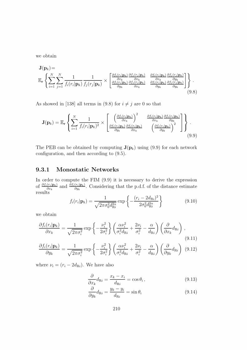
we obtain
J(pk)=
Er
{N∑
i=1
N∑
j=1
1
fi(ri|pk)
1
fj(rj |pk)×[
∂fi(ri|pk)∂xk
∂fj(rj |pk)
∂xk
∂fi(ri|pk)∂xk
∂fj(rj |pk)
∂yk∂fi(ri|pk)
∂yk
∂fj(rj |pk)
∂xk
∂fi(ri|pk)∂yk
∂fj(rj |pk)
∂yk
]}.
(9.8)
As showed in [138] all terms in (9.8) for i 6= j are 0 so that
J(pk) = Er
N∑
i=1
1
fi(ri|pk)2×
(
∂fi(ri|pk)∂xk
)2∂fi(ri|pk)
∂xk
∂fi(ri|pk)∂yk
∂fi(ri|pk)∂yk
∂fi(ri|pk)∂xk
(∂fi(ri|pk)
∂yk
)2
.
(9.9)
The PEB can be obtained by computing J(pk) using (9.9) for each networkconfiguration, and then according to (9.5).
9.3.1 Monostatic Networks
In order to compute the FIM (9.9) it is necessary to derive the expression
of ∂fi(ri|pk)∂xk
and ∂fi(ri|pk)∂yk
. Considering that the p.d.f. of the distance estimateresults
fi(ri|pk) =1√
2πσ20d
2αRi
exp
{−(ri − 2dRi)
2
2σ20d
2αRi
}(9.10)
we obtain
∂fi(ri|pk)
∂xk
=1√2πσ2
i
exp
{− ν2
i
2σ2i
}(αν2
i
σ2i dRi
+2νiσ2i
− α
dRi
)(∂
∂xk
dRi
),
(9.11)
∂fi(ri|pk)
∂yk=
1√2πσ2
i
exp
{− ν2
i
2σ2i
}(αν2
i
σ2i dRi
+2νiσ2i
− α
dRi
)(∂
∂ykdRi
)(9.12)
where νi = (ri − 2dRi). We have also
∂
∂xkdRi =
xk − xi
dRi= cos θi , (9.13)
∂
∂ykdRi =
yk − yidRi
= sin θi (9.14)
210

having indicated with θi the angle between the object and the ith receiver,measured with respect to the horizontal. We can now rewrite (9.9) as
J(pk) =N∑
i=1
Γi(dRi)
[cos2 θi cos θi sin θi
cos θi sin θi sin2 θi
](9.15)
where Γi(dRi) accounts for the expectation in (9.9) and is given by
Γi(dRi) =
∫ ∞
−∞
1
fi(ri|pk)g2i (νi) dνi (9.16)
with
gi(νi) =1√2πσ2
i
exp
{− ν2
i
2σ2i
}(αν2
i
σ2i dRi
+2νiσ2i
− α
dRi
). (9.17)
Substituting (9.17) in (9.16) the integral results
Γi(dRi) =4
σ2i
+2α2
d2Ri
. (9.18)
Moreover we can rewrite J in the form
J(pk) =
[∑Ni=1 J
(1)i (pk)
∑Ni=1 J
(2)i (pk)∑N
i=1 J(3)i (pk)
∑Ni=1 J
(4)i (pk)
]=
[ ∑Ni=1 Γi(dRi) cos
2 θi∑N
i=1 Γi(dRi) cos θi sin θi∑Ni=1 Γi(dRi) cos θi sin θi
∑Ni=1 Γi(dRi) sin
2 θi
]. (9.19)
The determinant of this matrix is given by
det J(pk) =
(N∑
i=1
Γi(dRi) cos2 θi
)(N∑
i=1
Γi(dRi) sin2 θi
)
−(
N∑
i=1
Γi(dRi) cos θi sin θi
)2
. (9.20)
Finally, it is so possible to derive J−1 as
J−1(pk) =1
detJ(pk)
×[ ∑N
i=1 Γi(dRi) sin2 θi −∑N
i=1 Γi(dRi) cos θi sin θi−∑N
i=1 Γi(dRi) cos θi sin θi∑N
i=1 Γi(dRi) cos2 θi
](9.21)
211
obtaining for the PEB the expression
PEB(pk) =√√√√√∑N
i=1 Γi(dRi)(∑Ni=1 Γi(dRi) cos2 θi
)(∑Ni=1 Γi(dRi) sin
2 θi
)−(∑N
i=1 Γi(dRi) cos θi sin θi
)2 .
(9.22)
This expression is formally equal to the one derived in [138] for active localiza-tion networks, with a different expression for the terms in (9.18) characteristicof these passive localization networks.
9.3.2 Multistatic Networks
For convenience of notation we rewrite (9.9) by introducing a double sumaccounting for the N = Nt × Nr observations due to the contribution of Nt
transmitters and Nr receivers, that is
J(pk) = Er
{Nr∑
i=1
Nt∑
j=1
1
fi,j(ri,j|pk)2
×
(∂fi,j(ri,j |pk)
∂xk
)2∂fi,j(ri,j |pk)
∂xk
∂fi,j(ri,j |pk)
∂yk
∂fi,j(ri,j |pk)
∂yk
∂fi,j(ri,j |pk)
∂xk
(∂fi,j(ri,j |pk)
∂yk
)2
(9.23)
where fi,j(ri,j|pk) is given by
fi,j(ri,j|pk)=1√
2πσ20d
αTjd
αRi
exp
{−(ri,j − dTj − dRi)
2
2σ20d
αTjd
αRi
}. (9.24)
The partial derivatives in (9.23) can be easily computed obtaining
∂fi,j(ri,j|pk)
∂xk
=1√2πσ2
i,j
exp
{− ν2
i,j
2σ2i,j
}
×[(
αν2i,j
2σ2i,jdTj
+νi,jσ2i,j
− α
2dTj
)(∂
∂xk
dTj
)
+
(αν2
i,j
2σ2i,jdRi
+νi,jσ2i,j
− α
2dRi
)(∂
∂xkdRi
)](9.25)
212

and
∂fi,j(ri,j|pk)
∂yk=
1√2πσ2
i,j
exp
{− ν2
i,j
2σ2i,j
}
×[(
αν2i,j
2σ2i,jdTj
+νi,jσ2i,j
− α
2dTj
)(∂
∂ykdTj
)
+
(αν2
i,j
2σ2i,jdRi
+νi,jσ2i,j
− α
2dRi
)(∂
∂ykdRi
)](9.26)
where νi,j = (ri,j − dTj − dRi). We have also
∂
∂xkdTj =
xk − xj
dTj= cos φj , (9.27)
∂
∂ykdTj =
yk − yjdTj
= sinφj (9.28)
having indicated with φj the angle between the jth transmitter and theobject, measured with respect to the horizontal.
Considering the structure of the matrix J(pk) in (9.23)
J(pk) =
[J1,1(pk) J1,2(pk)J2,1(pk) J2,2(pk)
](9.29)
we obtain the terms
J1,1(pk) =Nr∑
i=1
Nt∑
j=1
1√2πσ2
i,j
∫ ∞
−∞exp
{− ν2
i,j
2σ2i,j
}
× (kTj cosφj + kRi cos θi)2 dνi,j , (9.30)
J2,2(pk) =
Nr∑
i=1
Nt∑
j=1
1√2πσ2
i,j
∫ ∞
−∞exp
{− ν2
i,j
2σ2i,j
}
× (kTj sin φj + kRi sin θi)2 dνi,j , (9.31)
J1,2(pk) = J2,1(pk) =
Nr∑
i=1
Nt∑
j=1
1√2πσ2
i,j
∫ ∞
−∞exp
{− ν2
i,j
2σ2i,j
}
× (kTj cosφj + kRi cos θi) (kTj sin φj + kRi sin θi) dνi,j (9.32)
213

where
kTj =
(αν2
i,j
2σ2i,jdTj
+νi,jσ2i,j
− α
2dTj
)(9.33)
and
kRi =
(αν2
i,j
2σ2i,jdRi
+νi,jσ2i,j
− α
2dRi
). (9.34)
The integrals can be solved in closed form, obtaining:
J1,1(pk) =
Nr∑
i=1
Nt∑
j=1
[(1
σ2i,j
+α2
2d2Tj
)cos2 φj +
(1
σ2i,j
+α2
2d2Ri
)cos2 θi
+
(2
σ2i,j
+α2
dTjdRi
)cosφj cos θi
], (9.35)
J2,2(pk) =
Nr∑
i=1
Nt∑
j=1
[(1
σ2i,j
+α2
2d2Tj
)sin2 φj +
(1
σ2i,j
+α2
2d2Ri
)sin2 θi
+
(2
σ2i,j
+α2
dTjdRi
)sinφj sin θi
], (9.36)
J1,2(pk) = J2,1(pk) =Nr∑
i=1
Nt∑
j=1
[(1
σ2i,j
+α2
2d2Tj
)cosφj sinφj
+
(1
σ2i,j
+α2
2d2Ri
)cos θi sin θi
+
(1
σ2i
+α2
2dTjdRi
)sin (φj + θi)
]. (9.37)
We can now compute the PEB as
PEB(pk) =
√J1,1(pk) + J2,2(pk)
detJ(pk). (9.38)
Notice that if the jth transmitter is co-located with the ith receiver (i.e.,i = j, so with dTj = dRi and φj = θi) we have that the ith contributionsin (9.35), (9.36) and (9.37) degenerates, as expected, into the FIM elementsalready derived in (9.19).
214

9.4 Case Studies
We present, as case study, results in terms of the PEB derived in Sec. 9.3,related to TOA-based UWB-RFID localization. First we report, in Sec. 9.4.1,the system parameters considered in simulations necessary to determine theranging error at reference distance σ2
0 . Numerical evaluation of the PEBhas been carried out in a square cell of (20× 20)m2, with 4 reference nodesplaced at the corners if not differently specified. Specifically, 5 differentconfigurations are analyzed, showing as first the PEB in the 2D scenario(Sec. 9.4.2), and then the performance in terms of LEO (Sec. 9.4.3).
9.4.1 System Parameters
We consider a symbol composed of Ns = 8192 pulses11 with PRP Tp =200 ns. Transmitters and receivers have an antenna gain Gr = 2dBi, whiletags are equipped with an antenna with gainGt=1dBi.12 The backscatteringmodulation loss due to the presence of the switch in the tag is Lt = 2dB.The transmitted signal, adopting RRC pulses with pulse width parameterTw = 1ns, roll-off factor ν = 0.6, center frequency fc = 4GHz, is compliantwith the IEEE 802.15.4a emission mask in the 3.2−4.7GHz. The pathlosscoefficient and the receiver noise figure are, respectively, α=2 and F =4dB.
9.4.2 PEB in the 2D Scenario
Here we report the PEB mapped in the cell for each analyzed configuration.Note that we assume the same omnidirectional antennas for each case, whilethese can be optimized for any specific configuration.
Configuration #1. Figure 9.2 presents the PEB contour plot in the 2Dscenario adopting a monostatic configuration. It is interesting to notice thepresence of a wide central area where the localization error is almost con-stant to values close to 40 cm, which is quite interesting for many potentialapplications.
Configuration #2. Figure 9.3 reports the PEB considering an ideal multi-static configuration, where each receiver is able to process the signal emittedby each transmitter. In this case the localization performance is obviouslysignificantly improved with respect to the monostatic configuration, and theerror presents a different distribution in the 2D scenario. The best perfor-
11This is a typical value for the number of pulses per symbol [37].12We neglect frequency dependence as first approximation.
215

x [m]
y [m
]
0 2 4 6 8 10 12 14 16 18 200
2
4
6
8
10
12
14
16
18
20
0
0.1
0.2
0.3
0.4
0.5
0.6
0.7
0.8
0.9
1 [m]
Figure 9.2: Configuration #1. PEB considering 4 reference nodes (transceivers) at thecorners (monostatic).
x [m]
y [m
]
0 2 4 6 8 10 12 14 16 18 200
2
4
6
8
10
12
14
16
18
20
0
0.05
0.1
0.15
0.2
0.25
0.3
0.35
0.4 [m]
Figure 9.3: Configuration #2. PEB considering 4 reference nodes (transceivers) at thecorners, each processing the signals of every transmitter (multistatic).
mance is guarantee in the areas close to the reference nodes.13
Configuration #3. A different configuration is examined in Fig. 9.4, where
13Note that in this figure the scale is limited in the interval [0 − 0.4]m for a bettervisualization.
216

x [m]
y [m
]
0 2 4 6 8 10 12 14 16 18 200
2
4
6
8
10
12
14
16
18
20
0
0.1
0.2
0.3
0.4
0.5
0.6
0.7
0.8
0.9
1 [m]
Figure 9.4: Configuration #3. PEB considering 2 transmitters in [0, 0], [20, 20], and 2receivers in [20, 0], [0, 20] (multistatic).
two transmitters are placed in [0, 0] and [20, 20], and two receivers in the othertwo corners with coordinates [20, 0] and [0, 20]. Each receiver processes thesignal of both the transmitters, and the best coverage is again in the areasclose to the reference nodes. Moreover, it is interesting to notice that thereis no distinction, for what concern the localization capability, if a taggedobject is close to a transmitter or to a receiver. The performance is in generalworse than that in configurations #1 and #2 mainly because the number oftransmitter and receivers is halved.
Configurations #4 − 5. Other two multistatic configurations, with onlyone transmitter and 4 receivers, are investigated in Fig. 9.5 and Fig. 9.6.In configuration #4 the transmitter is co-located with the receiver in [0, 0],whereas in configuration #5 the transmitter is placed in the center of themonitored area in [10, 10]. As will be quantified in the next section, config-uration #5 is particularly attractive when a good compromise between thenumber of transmitters/receivers and localization coverage is desired.
9.4.3 Localization Error Outage
In order to compare the different topologies from the quantitative point ofview, we now analyze the performance in terms of LEO. In particular, theLEO is defined as the probability that the expected localization accuracy,where the expectation is taken over all the possible time instants and lo-
217

x [m]
y [m
]
0 2 4 6 8 10 12 14 16 18 200
2
4
6
8
10
12
14
16
18
20
0
0.1
0.2
0.3
0.4
0.5
0.6
0.7
0.8
0.9
1 [m]
Figure 9.5: Configuration #4. PEB considering 1 transmitter, in [0, 0], and 4 receivers atthe corners (multistatic).
cations, does not satisfy a threshold accuracy level ǫ [52, 28]. Figure 9.7reports the LEO as function of the target localization accuracy ǫ and for thedifferent configurations investigated in Sec. 9.4.2. It is possible to notice howthe multistatic configuration #2 with 4 transmitters and receivers ensuresthe highest performance in terms of outage achieving a target localizationaccuracy < 30 cm in almost all the locations of the area. The monostaticconfiguration #1 represents a trade-off among the investigated configura-tions, but cannot guarantee an error lower than about 35 cm in any locationwhen our system parameters are considered. The adoption of more directiveantennas can be an interesting solution for this specific case.
Differently, if we take into account configurations which employ a numberof transmitters lower than 4, configuration #5 represents an interesting so-lution which guarantees performance close to that of configuration #2 withthe advantage of a less power consuming network.
It is important to underline that the previous result did not account forthe effective network localization update rate, that is the frequency at whichthe network is able to refresh the position estimate of a certain target object[52]. In fact, considering a network adopting Nt transmitters working with aTDMA-based MAC, to guarantee the absence of mutual interference betweentransmitters, a new target location estimate is available after a time not lessthan NpNsNt seconds, that is, the time to transmit Nt ranging packets eachone composed of NpNs pulses. If now we assume to work with a network
218

x [m]
y [m
]
0 2 4 6 8 10 12 14 16 18 200
2
4
6
8
10
12
14
16
18
20
0
0.1
0.2
0.3
0.4
0.5
0.6
0.7
0.8
0.9
1 [m]
Figure 9.6: Configuration #5. PEB considering 1 transmitter in [10, 10], and 4 receiversat the corners (multistatic).
composed of a lower number of transmitters, as in configurations #3−5, thesame localization update rate can be guaranteed considering a symbol witha higher number of pulses Ns.
14 The corresponding increase of the effectiveSNR exploited by the receivers leads to a performance improvement. For afair comparison between configurations, Fig. 9.8 shows the LEO consideringthe same setting as in Fig. 9.7, where results are obtained at constant updaterate, that is, by considering Ns = 2 × 8192 for configuration #3 and Ns =4 × 8192 for configurations #4 − 5. In this setting, it is interesting to seehow the multistatic configuration #5, with one only transmitter placed at thecenter of the cell, is able to outperform also the multistatic case #2 with 4 co-located transmitters and receivers. Moreover, all multistatic configurationsoutperform the monostatic configuration #1.
It has to be remarked that results provided so far are related to per-formance bounds which serve as benchmarks for any practical localizationestimator as well as useful tools for identifying the best network deploymenttopology and configuration once the parameters are set as in Sec. 9.4.1. Inpractical setting, other issues must be taken into account, such as referencenodes synchronization, especially in multistatic configurations, and not omni-directional and frequency dependent object RCS. Reference nodes antennasgain and directivity play also an important role in the performance evaluationthat needs to be investigated.
14We consider the ranging packet composed of a fixed number of symbols.
219

0 0.1 0.2 0.3 0.4 0.5 0.6 0.7 0.8 0.9 10
0.1
0.2
0.3
0.4
0.5
0.6
0.7
0.8
0.9
1
ǫ [m]
LEO
Configuration #1Configuration #2Configuration #3Configuration #4Configuration #5
Figure 9.7: Localization error outage for different network configurations.
9.5 Conclusions
In this chapter theoretical bounds on the localization accuracy for non-cooperative objects (tagged and untagged) have been derived for monostaticand multistatic network configurations. These bounds are quite general andallow the investigation of the localization performance as a function of systemparameters, network topology and configuration. The case studies analyzedhave shown how the developed analytical framework is useful in identifyingthe best network topologies and configurations that maximize the localizationcoverage.
220

0 0.1 0.2 0.3 0.4 0.5 0.6 0.7 0.8 0.9 10
0.1
0.2
0.3
0.4
0.5
0.6
0.7
0.8
0.9
1
ǫ [m]
LEO
Configuration #1Configuration #2Configuration #3Configuration #4Configuration #5
Figure 9.8: Localization error outage for different network configurations when fixing thelocalization update rate.
221

222

Conclusions
This thesis covered different topics related to context-aware wireless networks,that are networks capable to adapt their behavior to the context and to theapplication, thanks to the possibility of enabling communication, sensing andlocalization, even considering active nodes and/or (semi-)passive nodes (i.e.,nodes not equipped with transmitters). Problems of signals demodulation,signal parameters estimation and localization have been addressed. In par-ticular low complexity solutions for demodulation and time-of-arrival (TOA)estimation, also adopting ultrawide-band (UWB) signals, have been investi-gated. The localization problem has been addressed from a practical pointof view, introducing solutions to cope with non-line-of-sight (NLOS) channelconditions. Novel radio-frequency identification (RFID) technologies havebeen investigated as case-study of context-aware wireless networks. Analyti-cal methods have been exploited to derive theoretical bounds and analyze, inclosed form, the performance of the proposed techniques. Experimentationhas been adopted for characterizing the performance of real networks and todevelop algorithms starting from real measured signals. Practical techniquesand ad-hoc system designs have been devised to deal with implementationissues or demand of low-complexity realizations.
Specifically, in Chapter 1 a new blind method for the determination ofthe integration time in non-coherent UWB receivers has been proposed. Itis based on information theoretic criteria (ITC) for model order selectionproblems, and it does not require any a priori knowledge or explicit featuresestimation from the propagation environment, as usual assumed with othertechniques. This allows exploiting part of the multipath channel diversitywithout adopting complex receiver architectures. In Chapter 2 novel non-coherent receiver structures, called stop-and-go (SaG) receivers, have been in-troduced and analyzed. This SaG strategy, based on energy detection, can beadopted with transmitted-reference (TR)-autocorrelation receivers (AcRs) orenergy detector receivers (EDRs), and it is able to further improve the signaldemodulation performance with respect to conventional receivers in clusteredmultipath channels, also in presence of synchronization errors. Moreover dif-
223

ferent optimization techniques, requiring different complexity and enablingdifferent receiver performance, have been proposed and characterized, pro-viding closed-form expressions for the receiver bit error probability (BEP).
In Chapter 3 the problem of time delay estimation (TDE) (or TOA es-timation) has been addressed from a theoretical point of view. This processis the key feature enabling network localization based on ranging measure-ments. Even if this issue has been widely investigate in the literature, nosignificant theoretical analyses are available in case of partial or no knowl-edge of the received signal waveform available. Along this direction, newfundamental bounds on TDE have been derived for different conditions, inparticular in the case the received signal is partially known or totally un-known at receiver side, as often occurs in practice due to multipath propaga-tion or due to the need of considering low-complexity estimators. Practicalestimators, such as energy-based estimators, have been revised in the contextof the novel theoretical derivation, and their performance compared with thenew bounds. This comparison has highlighted how the new bounds are verytight for all SNRs of interest, providing a new design method previously notavailable due to the impossibility of defining the Cramer-Rao bound (CRB)in the case of unknown signals. Thanks to the presented derivation the esti-mator performance can be, in fact, characterized analytically. The obtainedresults represent also a more general outcome with applications to differentsignal processing problems involving audio processing, source localization,and synchronization.
In Chapter 4 an experimentation methodology for the characterization ofcooperative localization networks in realistic indoor environments has beenintroduced. In the same chapter practical algorithms able to improve the ac-curacy in NLOS channel conditions have been proposed and tested on mea-surement databases realized during the experimentation. In particular it hasbeen shown using experimental data how it is possible to detect the presenceof LOS and NLOS channel conditions by a proper processing of the receivedwaveform, and how this information, as well as the prior knowledge of theenvironment map, can improve the localization accuracy. With the purposeof enhancing the localization coverage seriously compromised by the pres-ence of NLOS channel conditions, in Chapter 5 the idea of non-regenerativerelaying for network localization has been introduced. A system analysishas been presented and ad hoc position estimation techniques, accountingfor the presence of relay nodes in the network, have been devised. The casestudies investigated have highlighted the significant localization coverage im-provement achievable in NLOS conditions using the proposed low complexityrelaying scheme.
In Chapter 6 the concept of UWB-RFID systems for detecting and locat-
224
ing semi-passive tags based on backscatter modulation has been introducedas example of context-aware wireless network. Performance analysis for whatconcerns signal demodulation in ideal conditions and with ideal hardware hasbeen presented in Chapter 7, to assess the system feasibility. A deep studyinvolving low-complexity receiver structures and with hardware constraintshas been provided in Chapter 8. Specifically, receiver architectures able towork in realistic conditions and capable to deal with problems related tomulti-tag interference, synchronization mismatches and clock drift have beenintroduced and characterized in terms of performance. Moreover the maindesign challenges and practical solutions for implementation concerning re-ceiver dynamic range, A/D conversion, synchronization and multiple accesshave been investigated. Finally, theoretical bounds on the localization accu-racy of RFID-UWB systems have been derived in Chapter 9. These boundsare useful to characterize not only the RFID-UWB network from the pointof view of the localization accuracy, but can be also applied to other passivelocalization networks such wireless sensor radars (WSRs). In particular thebehavior of different network configurations can be described, allowing thecharacterization of monostatic, bistatic and multistatic networks.
Several issues investigated in this thesis are under extension for furtherpublications. In particular, for what concerns the problem of TDE, the intro-duction of non-idealities on the signal model, such as fading and interferenceeffects will be considered in the future in the analysis of theoretical bounds.This allows describing in analytic form the behavior of non-coherent TOAestimators in presence of these effects. The introduction of the same non-idealities can be considered for deriving the BEP expressions characterizingthe SaG receivers proposed in Chapter 2. In the field of location-awareness,novel experimental campaigns, started from the work carried out at MIT, arein preparation in order to test different localization algorithms in differentoperating scenarios under a common database. Moreover the feasibility ofthe relaying scheme will be proved with experimental measurements in re-alistic propagation conditions, in cooperation with CEA-LETI, a partner ofthe European project SELECT. The different components of the UWB-RFIDsystem and the signal processing tasks introduced and analyzed are currentlyunder development and a proof of concept of the feasibility of this system willbe provided in the following months within the European project SELECT.The framework developed so far for passive localization can represent a start-ing point for further investigations on localization networks involving activeand passive tags or offering WSR functionalities in conjunction with multi-static approaches. Finally, as introduced in Chapter 6, multistatic techniquescan be investigated in the UWB-RFID system not only for tags localization,but also for enhanced detection and robust tag to reader communication.
225

226

Bibliography
[1] C. Floerkemeier, M. Langheinrich, E. Fleisch, F. Mattern, and S. E.Sarma, Eds., The Internet of Things. Springer, March. 2008.
[2] A. Iera, C. Floerkemeier, J. Mitsugi, and G. Morabito, “The Internetof Things,” IEEE Wireless Communications, vol. 17, no. 6, pp. 8 –9,Dec. 2010.
[3] J. Zheng, D. Simplot-Ryl, C. Bisdikian, and H. Mouftah, “The Internetof Things,” IEEE Commun. Mag., vol. 49, no. 11, pp. 30 –31, Nov.2011.
[4] K. Finkenzeller, RFID Handbook: Fundamentals and Applications inContactless Smart Cards and Identification. Wiley, 2004.
[5] M. Weiser, “The computer for the 21st century,” Scientific American,vol. 265, no. 3, pp. 94–104, 1991.
[6] B. Schilit, N. Adams, and R. Want, “Context-aware computing appli-cations,” in First Workshop on Mobile Computing Systems and Appli-cations. IEEE, 1994, pp. 85–90.
[7] G. Chen and D. Kotz, “A survey of context-aware mobile computingresearch,” Technical Report TR2000-381, Dept. of Computer Science,Dartmouth College, Tech. Rep., 2000.
[8] V. Pejovic and E. Belding, “A context-aware approach to wirelesstransmission adaptation,” in 8th Annual IEEE Communications So-ciety Conference on Sensor, Mesh and Ad Hoc Communications andNetworks (SECON). IEEE, 2011, pp. 592–600.
[9] A. Wood, J. Stankovic, G. Virone, L. Selavo, Z. He, Q. Cao, T. Doan,Y. Wu, L. Fang, and R. Stoleru, “Context-aware wireless sensor net-works for assisted living and residential monitoring,” IEEE Network,vol. 22, no. 4, pp. 26–33, 2008.
227
[10] M. Covington, P. Fogla, Z. Zhan, and M. Ahamad, “A context-awaresecurity architecture for emerging applications,” in 18th Annual Com-puter Security Applications Conference. IEEE, 2002, pp. 249–258.
[11] H. van Kranenburg, M. Bargh, S. Iacob, and A. Peddemors, “A contextmanagement framework for supporting context-aware distributed ap-plications,” IEEE Communications Magazine, vol. 44, no. 8, pp. 67–74,2006.
[12] D. Bottazzi, A. Corradi, and R. Montanari, “Context-aware middle-ware solutions for anytime and anywhere emergency assistance to el-derly people,” IEEE Communications Magazine, vol. 44, no. 4, pp.82–90, 2006.
[13] H. Pung, T. Gu, W. Xue, P. Palmes, J. Zhu, W. Ng, C. Tang, andN. Chung, “Context-aware middleware for pervasive elderly homecare,”IEEE Journal on Selected Areas in Communications, vol. 27, no. 4, pp.510–524, 2009.
[14] A. Krause, A. Smailagic, and D. Siewiorek, “Context-aware mobilecomputing: Learning context-dependent personal preferences from awearable sensor array,” IEEE Transactions on Mobile Computing,vol. 5, no. 2, pp. 113–127, 2006.
[15] Z. Yu, X. Zhou, Z. Yu, D. Zhang, and C. Chin, “An OSGi-based infras-tructure for context-aware multimedia services,” IEEE communicationsMagazine, vol. 44, no. 10, pp. 136–142, 2006.
[16] A. Smailagic and D. Kogan, “Location sensing and privacy in acontext-aware computing environment,” IEEE Wireless Communica-tions, vol. 9, no. 5, pp. 10–17, 2002.
[17] T. Kanter, “Hottown, enabling context-aware and extensible mobileinteractive spaces,” IEEE Wireless Communications, vol. 9, no. 5, pp.18–27, 2002.
[18] P. Bellavista, A. Corradi, and C. Giannelli, “A unifying perspectiveon context-aware evaluation and management of heterogeneous wire-less connectivity,” IEEE Communications Surveys & Tutorials, vol. 13,no. 3, pp. 337–357, 2011.
[19] K. Rehman, F. Stajano, and G. Coulouris, “An architecture for inter-active context-aware applications,” IEEE Pervasive Computing, vol. 6,no. 1, pp. 73–80, 2007.
228

[20] M. van Sinderen, A. van Halteren, M. Wegdam, H. Meeuwissen, andE. Eertink, “Supporting context-aware mobile applications: an infras-tructure approach,” IEEE Communications Magazine, vol. 44, no. 9,pp. 96–104, 2006.
[21] J. Garcia-luna aceves, M. Mosko, I. Solis, R. Braynard, and R. Ghosh,“Context-aware protocol engines for ad hoc networks,” IEEE Commu-nications Magazine, vol. 47, no. 2, pp. 142–149, 2009.
[22] P. Makris, D. Skoutas, and C. Skianis, “A survey on context-awaremobile and wireless networking: On networking and computing envi-ronments’ integration,” 2012.
[23] B. Schilit, D. Hilbert, and J. Trevor, “Context-aware communication,”IEEE Wireless Communications, vol. 9, no. 5, pp. 46–54, 2002.
[24] D. Dardari, E. Falletti, and M. Luise, Satellite and Terrestrial RadioPositioning Techniques - A signal processing perspective. Elsevier Ltd,London, 2011.
[25] N. Decarli, A. Giorgetti, D. Dardari, and M. Chiani, “Blind integrationtime determination for UWB transmitted reference receivers,” in Proc.IEEE Global Telecomm. Conf., Dec. 2011, pp. 1 –5.
[26] N. Decarli, A. Giorgetti, D. Dardari, M. Chiani, and M. Z. Win, “Stop-and-go receivers for non-coherent UWB communication,” IEEE Trans.Wireless Commun., 2013, submitted.
[27] N. Decarli, D. Dardari, and M. Win, “Bounds on time-delay estimationof partially known and unknown signals,” 2013, in preparation.
[28] A. Conti, M. Guerra, D. Dardari, N. Decarli, and M. Z. Win, “Networkexperimentation for cooperative localization,” IEEE J. Select. AreasCommun., vol. 30, no. 2, pp. 467–475, Feb. 2012.
[29] N. Decarli, D. Dardari, S. Gezici, and A. D’Amico, “LOS/NLOS detec-tion for UWB signals: a comparative study using experimental data,”in IEEE International Symposium on Wireless Pervasive Computing(ISWPC 2010), Modena, Italy, May 2010.
[30] D. Dardari, N. Decarli, A. Guerra, and A. Conti, “Enhanced localiza-tion coverage with non-regenerative UWB relays,” in 20th EuropeanSignal Processing Conference (EUSIPCO), Bucharest, Romania, Aug.2012.
229
[31] N. Decarli, A. Guerra, A. Conti, R. D’Errico, A. Sibille, and D. Dard-ari, “Non-regenerative relaying for network localization,” IEEE Trans.Wireless Commun., 2013, submitted.
[32] N. Decarli, F. Guidi, A. Conti, and D. Dardari, “Interference and clockdrift effects in UWB RFID systems using backscatter modulation,”in IEEE International Conference on Ultra-Wideband, ICUWB 2012,Syracuse, USA, Sep. 2012, pp. 1–5.
[33] F. Guidi, N. Decarli, D. Dardari, C. Roblin, and A. Sibille, “Perfor-mance of UWB backscatter modulation in multi-tag RFID scenariousing experimental data,” in IEEE International Conference on Ultra-Wideband, ICUWB 2011, Bologna, Italy, Sep. 2011, pp. 1–5.
[34] R. D’Errico, M. Bottazzi, F. Natali, E. Savioli, S. Bartoletti, A. Conti,D. Dardari, N. Decarli, F. Guidi, F. Dehmas, L. Ouvry, U. Al-varado, N. Hadaschik, C. Franke, Z. Mhanna, M. Sacko, Y. Wei,and A. Sibille, “An UWB-UHF semi-passive RFID system for local-ization and tracking applications,” in IEEE International Conferenceon RFID-Technologies and Applications (RFID-TA), Nov. 2012, pp. 18–23.
[35] N. Decarli and D. Dardari, “RFID and radar localization: A positionerror bound analysis,” in Proc. IEEE Int. Conf. on Commun., Jun.2013.
[36] E. Savioli, M. Bottazzi, F. Natali, N. Decarli, F. Guidi, N. Hadaschik,R. D’Errico, and L. Ouvry, “Semi-passive UHF-UWB RFID: Archi-tecture and localization performance,” in Proc. IEEE Int. Conf. onCommun., Jun. 2013.
[37] F. Guidi, N. Decarli, S. Bartoletti, A. Conti, and D. Dardari, “Ro-bust detection of UWB backscatter signals in multi-tag environments,”2013, in preparation.
[38] N. Decarli, F. Guidi, and D. Dardari, “A novel joint RFID andradar sensor network for passive localization: Design and performancebounds,” IEEE J. Sel. Topics in Signal Processing, 2013, submitted.
[39] “EUWB D2.2.2; Interference identification algorithms,” Mar. 2010.
[40] “EUWB D2.4.2; Interference mitigation techniques algorithms,” Jul.2010.
230

[41] “NEWCOM DRB.4; Final report: seamless positioning techniques inwireless communications,” Dec. 2011.
[42] “SELECT D2.1.1; Backscatter propagation modeling: interim report,”Jul. 2011.
[43] “SELECT D2.2.1; Signal processing techniques: interim report,” Jul.2011.
[44] “SELECT D2.3.1; Multi-functional network design: intermediate sys-tem specification,” Sep. 2011.
[45] “SELECT D2.2.2; Signal processing techniques: final report,” Apr.2012.
[46] “SELECT D2.3.2; Multi-functional network design: final system spec-ification,” Jun. 2012.
[47] M. Z. Win and R. A. Scholtz, “Impulse radio: How it works,” IEEECommun. Lett., vol. 2, no. 2, pp. 36–38, Feb. 1998.
[48] ——, “Ultra -wide bandwidth time -hopping spread-spectrum impulseradio for wireless multiple -access communications,” IEEE Trans. Com-mun., vol. 48, no. 4, pp. 679–691, Apr. 2000.
[49] M. Win, D. Dardari, A. Molisch, W. Wiesbeck, and J. Zhang, “Historyand applications of UWB,” Proc. IEEE, vol. 97, no. 2, pp. 198 –204,Feb. 2009.
[50] D. Dardari, R. D’Errico, C. Roblin, A. Sibille, and M. Z. Win, “Ul-trawide bandwidth RFID: The next generation?” Proceedings of theIEEE, Special Issue on RFID - A Unique Radio Innovation for the21st Century., vol. 98, no. 9, pp. 1570 –1582, Sep. 2010.
[51] D. Dardari, A. Conti, U. Ferner, A. Giorgetti, and M. Win, “Rangingwith ultrawide bandwidth signals in multipath environments,” Proceed-ings of the IEEE, vol. 97, no. 2, pp. 404 –426, Feb. 2009.
[52] M. Z. Win, A. Conti, S. Mazuelas, Y. Shen, W. M. Gifford, D. Dardari,and M. Chiani, “Network localization and navigation via cooperation,”IEEE Commun. Mag., vol. 49, no. 5, pp. 56–62, May 2011.
[53] M. Z. Win and R. A. Scholtz, “On the robustness of ultra -wide band-width signals in dense multipath environments,” IEEE Commun. Lett.,vol. 2, no. 2, pp. 51–53, Feb. 1998.
231

[54] ——, “On the energy capture of ultra -wide bandwidth signals in densemultipath environments,” IEEE Commun. Lett., vol. 2, no. 9, pp. 245–247, Sep. 1998.
[55] ——, “Characterization of ultra -wide bandwidth wireless indoor com-munications channel: A communication theoretic view,” IEEE J.Select. Areas Commun., vol. 20, no. 9, pp. 1613–1627, Dec. 2002, .
[56] D. Cassioli, M. Z. Win, and A. F. Molisch, “The ultra -wide bandwidthindoor channel: from statistical model to simulations,” IEEE J. Select.Areas Commun., vol. 20, no. 6, pp. 1247–1257, Aug. 2002.
[57] A. Molisch, “Ultra-wide-band propagation channels,” Proc. IEEE,vol. 97, no. 2, pp. 353 –371, Feb. 2009.
[58] M. Win, G. Chrisikos, and N. Sollenberger, “Performance of RAKEreception in dense multipath channels: implications of spreading band-width and selection diversity order,” IEEE J. Select. Areas Commun.,vol. 18, no. 8, pp. 1516 –1525, Aug. 2000.
[59] V. Lottici, A. D’Andrea, and U. Mengali, “Channel estimation forultra-wideband communications,” IEEE J. Select. Areas Commun.,vol. 20, no. 9, pp. 1638–1645, Dec. 2002.
[60] K. Witrisal, G. Leus, G. Janssen, M. Pausini, F. Troesch, T. Zasowski,and J. Romme, “Noncoherent ultra-wideband systems,” IEEE SignalProcessing Magazine, vol. 26, no. 4, pp. 48 –66, Jul. 2009.
[61] J. G. Proakis, Digital Communications, 4th ed. New York, NY, 10020:McGraw-Hill, Inc., 2001.
[62] D. Torrieri, Principles of Spread Spectrum Communication Systems.Springer, 2005.
[63] A. F. Molisch, Wireless Communications, 1st ed. Piscataway, NewJersey, 08855-1331: IEEE Press, J. Wiley and Sons, 2005.
[64] J. J. Stiffler, Theory of Synchronous Communications, 1st ed. Engle-wood Cliffs, New Jersey 07632: Prentice-Hall, 1971.
[65] B. Sklar, Digital communications: fundamentals and applications, ser.Prentice Hall Communications Engineering and Emerging TechnologiesSeries. Prentice-Hall PTR, 2001.
232

[66] H. L. V. Trees, Detection, Estimation, and Modulation Theory: PartI, 2nd ed. New York, NY: John Wiley & Sons, Inc., 2001.
[67] C. K. Rushforth, “Transmitted-reference techniques for random or un-known channels,” IEEE Trans. Inform. Theory, vol. 10, pp. 39 – 42,Jan. 1964.
[68] A. Polydoros and K. T. Woo, “LPI detection of frequency-hoppingsignals using autocorrelation techniques,” IEEE J. Select. Areas Com-mun., vol. 3, no. 5, pp. 714 – 726, Sep. 1985.
[69] J. D. Choi and W. E. Stark, “Performance of ultra-wideband commu-nications with suboptimal receivers in multipath channels,” IEEE J.Select. Areas Commun., vol. 20, no. 9, pp. 1754–1766, Dec. 2002.
[70] Y.-L. Chao and R. A. Scholtz, “Ultra-wideband transmitted referencesystems,” IEEE Trans. Veh. Technol., vol. 54, no. 5, pp. 1556–1569,Sep. 2005.
[71] S. Niranjayan and N. Beaulieu, “General performance analysis of TRUWB systems,” IEEE Trans. Wireless Commun., vol. 7, no. 12, pp.5268 –5277, Dec. 2008.
[72] T. Q. S. Quek, M. Z. Win, and D. Dardari, “Unified analysis of UWBtransmitted-reference schemes in the presence of narrowband interfer-ence,” IEEE Trans. Wireless Commun., vol. 6, no. 6, pp. 2126–2139,Jun. 2007.
[73] A. Rabbachin, T. Quek, P. Pinto, I. Oppermann, and M. Win, “Non-coherent UWB communication in the presence of multiple narrowbandinterferers,” IEEE Trans. Wireless Commun., vol. 9, no. 11, pp. 3365–3379, Nov. 2010.
[74] T. Jia and D. I. Kim, “Multiple access performance of balanced UWBtransmitted-reference systems in multipath,” IEEE Trans. WirelessCommun., vol. 7, no. 3, pp. 1084 –1094, Mar. 2008.
[75] D. Goeckel and Q. Zhang, “Slightly frequency-shifted reference ultra-wideband (UWB) radio,” IEEE Transactions on Communications,vol. 55, no. 3, pp. 508 –519, Mar. 2007.
[76] A. D’amico and U. Mengali, “Code-multiplexed UWB transmitted-reference radio,” IEEE Transactions on Communications, vol. 56,no. 12, pp. 2125 –2132, Dec. 2008.
233

[77] X. Dong, L. Jin, and P. Orlik, “A new transmitted reference pulsecluster system for UWB communications,” IEEE Trans. Veh. Technol.,vol. 57, no. 5, pp. 3217 –3224, Sep. 2008.
[78] T. Quek, M. Win, and D. Dardari, “Unified analysis of UWBtransmitted-reference schemes in the presence of narrowband interfer-ence,” IEEE Transactions on Wireless Communications, vol. 6, no. 6,pp. 2126 –2139, Jun. 2007.
[79] S. Franz and U. Mitra, “Integration interval optimization and perfor-mance analysis for UWB transmitted reference systems,” in Interna-tional Workshop on Ultra Wideband Systems, 2004., May 2004, pp. 26– 30.
[80] Y.-L. Chao, “Optimal integration time for UWB transmitted refer-ence correlation receivers,” in Conference Record of the Thirty-EighthAsilomar Conference on Signals, Systems and Computers, 2004., vol. 1,2004, pp. 647 – 651.
[81] M. Nemati, U. Mitra, and R. Scholtz, “Optimum integration time forUWB transmitted reference and energy detector receivers,” in IEEEMilitary Communications Conference, 2006. MILCOM 2006., 2006.
[82] C.-H. Hsieh, W-D.Wu, and C.-C. Chao, “Optimal channel energycapture for ultra-wideband transmitted reference systems in clusteredchannels,” in IEEE Wireless Communications and Networking Confer-ence (WCNC), 2010, 2010, pp. 1 –6.
[83] Y. Na and M. Saquib, “Analysis of the channel energy capture in ultra-wideband transmitted reference systems,” IEEE Transactions on Com-munications, vol. 55, no. 2, pp. 262 –265, 2007.
[84] R. Zhang and X. Dong, “Synchronization and integration region op-timization for UWB signals with non-coherent detection and auto-correlation detection,” IEEE Transactions on Communications, vol. 56,no. 5, pp. 790 –798, May 2008.
[85] L. Jin, X. Dong, and Z. Liang, “Integration interval determination algo-rithms for ber minimization in UWB transmitted reference pulse clus-ter systems,” IEEE Transactions on Wireless Communications, vol. 9,no. 8, pp. 2408 –2414, 2010.
[86] H. Urkowitz, “Energy detection of unknown deterministic signals,”Proceedings of the IEEE, vol. 55, no. 4, pp. 523 – 531, 1967.
234

[87] P. Stoica and Y. Selen, “Model-order selection: a review of informationcriterion rules,” IEEE Signal Processing Mag., vol. 21, no. 4, pp. 36–47,2004.
[88] M. Chiani and M. Win, “Estimating the number of signals observedby multiple sensors,” in 2nd International Workshop on Cognitive In-formation Processing (CIP), 2010. IEEE, 2010, pp. 156–161.
[89] A. Giorgetti and M. Chiani, “A new approach to time-of-arrival esti-mation based on information theoretic criteria,” in IEEE Int. Conf. onUltra-Wideband (ICUWB 2011, Bologna, Italy, Sep. 2011, pp. 1–5.
[90] K. M. L. Saxena and K. Alam, “Estimation of the non-centralityparameter of a Chi squared distribution,” The Annals of Statistics,vol. 10, no. 3, pp. 1012–1016, 1982.
[91] H. Bozdogan, “Model selection and Akaike’s information criterion(AIC): The general theory and its analytical extensions,” Psychome-trika, vol. 52, no. 3, pp. 345–370, 1987.
[92] A. Molisch, K. Balakrishnan, D. Cassioli, C.-C. Chong, S. Emami,A. Fort, J. Karedal, J. Kunisch, H. Schantz, U. Schuster, and K. Siwiak,“IEEE 802.15.4a channel model - final report,” 2005.
[93] M. Sahin, I. Guvenc, and H. Arslan, “Optimization of energy detectorreceivers for UWB systems,” in IEEE 61st Vehicular Technology Con-ference, 2005. VTC 2005-Spring, vol. 2, Jun. 2005, pp. 1386 – 1390.
[94] F. Wang, Z. Tian, and B. Sadler, “Weighted energy detection for non-coherent ultra-wideband receiver design,” IEEE Trans. Wireless Com-mun., vol. 10, no. 2, pp. 710 –720, Feb. 2011.
[95] A. D’Amico, U. Mengali, and E. Arias-de Reyna, “Energy-detectionUWB receivers with multiple energy measurements,” IEEE Transac-tions on Wireless Communications, vol. 6, no. 7, pp. 2652 –2659, Jul.2007.
[96] G. Leus and A.-J. van der Veen, “A weighted autocorrelation receiverfor transmitted reference ultra wideband communications,” in IEEE6th Workshop on Signal Processing Advances in Wireless Communica-tions, Jun. 2005, pp. 965 – 969.
[97] J. Wu, H. Xiang, and Z. Tian, “Weighted noncoherent receivers forUWB PPM signals,” IEEE Communications Letters, vol. 10, no. 9,pp. 655 –657, sept. 2006.
235

[98] D. Mu and Z. Qiu, “Weighted non-coherent energy detection receiverfor UWB OOK systems,” in 9th International Conference on SignalProcessing, 2008. ICSP 2008, Oct. 2008, pp. 1846 –1849.
[99] J. Romme and K. Witrisal, “Transmitted-reference UWB systems usingweighted autocorrelation receivers,” IEEE Transactions on MicrowaveTheory and Techniques, vol. 54, no. 4, pp. 1754 – 1761, Jun. 2006.
[100] D. Dardari, A. Giorgetti, M. Chiani, T. Quek, and M. Win, “A stop-and-go transmitted-reference UWB receiver,” in IEEE InternationalConference on Ultra-Wideband, Sep. 2006, pp. 309 –314.
[101] T. Quek and M. Win, “Ultrawide bandwidth transmitted-reference sig-naling,” in IEEE International Conference on Communications, vol. 6,Jun. 2004, pp. 3409 – 3413.
[102] ——, “Analysis of UWB transmitted-reference communication systemsin dense multipath channels,” IEEE J. Select. Areas Commun., vol. 23,no. 9, pp. 1863 – 1874, 2005.
[103] A. D’Amico, U. Mengali, and L. Taponecco, “Synchronization for dif-ferential transmitted reference UWB receivers,” IEEE Trans. WirelessCommun., vol. 6, no. 11, pp. 4154 –4163, Nov. 2007.
[104] S. Franz, C. Carnonelli, and U. Mitra, “Joint semi-blind channel andtiming estimation for generalized UWB transmitted reference systems,”IEEE Trans. Wireless Commun., vol. 6, no. 1, pp. 180 –191, Jan. 2007.
[105] A. F. Molisch, “Ultrawideband propagation channels-theory, measure-ments, and modeling,” IEEE Trans. Veh. Technol., vol. 54, no. 5, pp.1528–1545, Sep. 2005.
[106] M. Abramowitz and I. A. Stegun, Handbook of Mathematical Functionswih Formulas, Graphs, and Mathematical Tables. Washington, D.C.:United States Department of Commerce, 1970.
[107] S. Dubouloz, B. Denis, S. de Rivaz, and L. Ouvry, “Performance analy-sis of LDR UWB non-coherent receivers in multipath environments,” inIEEE International Conference on Ultra-Wideband, 2005., Sep. 2005.
[108] H. Akaike, “A new look at the statistical model identification,” IEEETrans. Automat. Contr., vol. 19, no. 6, pp. 716–723, Dec. 1974.
[109] J. Rissanen, “Modeling by shortest data description,” Automatica,vol. 14, no. 5, pp. 465–471, 1978.
236
[110] A. Giorgetti and M. Chiani, “Time-of-arrival estimation based on in-formation theoretic criteria,” IEEE Trans. on Signal Processing, 2013.
[111] A. Mariani, A. Giorgetti, and M. Chiani, “Effects of noise power es-timation on energy detection for cognitive radio applications,” IEEETrans. Commun., vol. 59, no. 12, pp. 3410 –3420, Dec. 2011.
[112] G. Schwarz, “Estimating the dimension of a model,” The annals ofstatistics, vol. 6, no. 2, pp. 461–464, 1978.
[113] “IEEE standard for information technology - telecommunications andinformation exchange between systems - local and metropolitan areanetworks - specific requirement part 15.4: Wireless medium accesscontrol (MAC) and physical layer (PHY) specifications for low-ratewireless personal area networks (WPANs),” IEEE Std 802.15.4a-2007(Amendment to IEEE Std 802.15.4-2006), pp. 1–203, 2007.
[114] A. F. Molisch, D. Cassioli, C.-C. Chong, S. Emami, A. Fort, B. Kan-nan, J. Karedal, J. Kunisch, H. Schantz, K. Siwiak, and M. Z. Win,“A comprehensive standardized model for ultrawideband propagationchannels,” IEEE Trans. Antennas Propagat., vol. 54, no. 11, pp. 3151–3166, Nov. 2006, Special Issue on Wireless Communications.
[115] G. Carter, “Coherence and time delay estimation,” Proceedings of theIEEE, vol. 75, no. 2, pp. 236–255, 1987.
[116] A. J. Weiss and E. Weinstein, “Fundamental limitations in passive timedelay estimation - part I: Narrow-band systems,” IEEE Trans. Acoust.,Speech, Signal Processing, vol. ASP-31, no. 2, pp. 472–486, Apr. 1983.
[117] J. P. Iannello, “Large and small error performance limits for multipathtime delay estimation,” IEEE Trans. Acoust., Speech, Signal Process-ing, vol. ASSP-34, no. 2, pp. 245–251, Apr. 1986.
[118] J. Li and R. Wu, “An efficient algorithm for time delay estimation,”IEEE Trans. Signal Processing, vol. 46, no. 8, pp. 2231–2235, Aug.1998.
[119] T. Manickam, R. Vaccaro, and D. Tufts, “A least-squares algorithmfor multipath time-delay estimation,” IEEE Trans. Signal Processing,vol. 42, no. 11, pp. 3229–3233, 1994.
[120] J. Stuller and N. Hubing, “New perspectives for maximum likeli-hood time-delay estimation,” IEEE Transactions on Signal Processing,vol. 45, no. 3, pp. 513–525, 1997.
237

[121] G. Jacovitti and G. Scarano, “Discrete time techniques for time delayestimation,” IEEE Transactions on Signal Processing, vol. 41, no. 2,pp. 525–533, 1993.
[122] B. Sadler and R. Kozick, “A survey of time delay estimation perfor-mance bounds,” in Fourth IEEE Workshop on Sensor Array and Mul-tichannel Processing. IEEE, 2006, pp. 282–288.
[123] K. Gedalyahu and Y. Eldar, “Time-delay estimation from low-rate sam-ples: A union of subspaces approach,” IEEE Transactions on SignalProcessing, vol. 58, no. 6, pp. 3017–3031, 2010.
[124] C. Knapp and G. Carter, “The generalized correlation method for es-timation of time delay,” IEEE Transactions on Acoustics, Speech andSignal Processing, vol. 24, no. 4, pp. 320–327, 1976.
[125] J. Krolik, M. Eizenman, and S. Pasupathy, “Time delay estimationof signals with uncertain spectra,” IEEE Transactions on Acoustics,Speech and Signal Processing, vol. 36, no. 12, pp. 1801–1811, 1988.
[126] B. Yegnanarayana, S. Prasanna, R. Duraiswami, and D. Zotkin, “Pro-cessing of reverberant speech for time-delay estimation,” IEEE Trans-actions on Speech and Audio Processing, vol. 13, no. 6, pp. 1110–1118,2005.
[127] H. Urkowitz, C. Hauer, and J. Koval, “Generalized resolution in radarsystems,” Proceedings of the IRE, vol. 50, no. 10, pp. 2093–2105, 1962.
[128] M. Zakai and J. Ziv, “On the threshold effect in radar range estimation(corresp.),” IEEE Transactions on Information Theory, vol. 15, no. 1,pp. 167–170, 1969.
[129] G. Carter, “Time delay estimation for passive sonar signal processing,”IEEE Transactions on Acoustics, Speech and Signal Processing, vol. 29,no. 3, pp. 463–470, 1981.
[130] A. Tajer, G. Jajamovich, X. Wang, and G. Moustakides, “Optimal jointtarget detection and parameter estimation by MIMO radar,” IEEEJournal of Selected Topics in Signal Processing, vol. 4, no. 1, pp. 127–145, 2010.
[131] B. Friedlander, “An efficient parametric technique for doppler-delayestimation,” IEEE Transactions on Signal Processing, vol. 60, no. 8,pp. 3953–3963, 2012.
238

[132] C. Carbonelli and U. Mengali, “Synchronization algorithms for UWBsignals,” IEEE Transactions on Communications, vol. 54, no. 2, pp.329 – 338, Feb. 2006.
[133] C. Carbonelli, U. Mengali, and U. Mitra, “Synchronization and chan-nel estimation for UWB signal,” in IEEE Global TelecommunicationsConference, GLOBECOM, vol. 2, Dec. 2003, pp. 764 – 768 Vol.2.
[134] S. Gezici, Z. Tian, G. B. Giannakis, H. Kobayashi, A. F. Molisch,H. V. Poor, and Z. Sahinoglu, “Localization via ultra-wideband radios:a look at positioning aspects for future sensor networks,” IEEE SignalProcessing Mag., vol. 22, pp. 70–84, Jul. 2005.
[135] D. Dardari, C.-C. Chong, and M. Z. Win, “Threshold-based time-of-arrival estimators in UWB dense multipath channels,” IEEE Trans.Commun., vol. 56, 2008.
[136] Y. Shen and M. Z. Win, “Fundamental limits of wideband localization– Part I: A general framework,” IEEE Trans. Inform. Theory, vol. 56,2010.
[137] Y. Shen, H. Wymeersch, and M. Z. Win, “Fundamental limits of wide-band localization – Part II: Cooperative networks,” IEEE Trans. In-form. Theory, vol. 56, 2010.
[138] D. B. Jourdan, D. Dardari, and M. Z. Win, “Position error boundfor UWB localization in dense cluttered environments,” IEEE Trans.Aerosp. Electron. Syst., vol. 44, no. 2, pp. 613–628, Apr. 2008.
[139] K. Yu and I. Oppermann, “An ultra wideband TAG circuit transceiverarchitecture,” in International Workshop on Ultra Wideband Systems.Joint UWBST and IWUWBS 2004., Kyoto, Japan, May 2004, pp.258–262.
[140] S. Gezici, Z. Sahinoglu, H. Kobayashi, and H. V. Poor, UltrawidebandWireless Communications. John Wiley & Sons, Inc., 2006, ch. UltraWideband Geolocation.
[141] J. Ianniello, “High-resolution multipath time delay estimation forbroad-band random signals,” IEEE Transactions on Acoustics, Speechand Signal Processing, vol. 36, no. 3, pp. 320–327, 1988.
[142] O. Bialer, D. Raphaeli, and A. Weiss, “Efficient time of arrival esti-mation algorithm achieving maximum likelihood performance in dense
239

multipath,” IEEE Transactions on Signal Processing, vol. 60, no. 3,pp. 1241–1252, 2012.
[143] J.-Y. Lee and R. A. Scholtz, “Ranging in a dense multipath environ-ment using an UWB radio link,” IEEE J. Select. Areas Commun.,vol. 20, no. 9, pp. 1677–1683, Dec. 2002.
[144] I. Guvenc and Z. Sahinoglu, “Threshold-based TOA estimation forimpulse radio UWB systems,” in Proc. IEEE Int. Conf. on Ultra-Wideband (ICUWB), Zurich, Switzerland, 2005, pp. 420–425.
[145] A. D’Amico, U. Mengali, and L. Taponecco, “Energy-based TOA es-timation,” IEEE Transactions on Wireless Communications, vol. 7,no. 3, pp. 838 –847, mar 2008.
[146] A. Rabbachin, I. Oppermann, and B. Denis, “ML time-of-arrival es-timation based on low complexity UWB energy detection,” in Proc.IEEE Int. Conf. on Ultra-Wideband (ICUWB), Waltham, MA, Sep2006, pp. 599–604.
[147] ——, “GML ToA estimation based on low complexity UWB energydetection,” in Proc. IEEE Int. Symp. on Personal, Indoor and MobileRadio Commun., Sep. 2006, pp. 1 –5.
[148] Z. Lei, F. Chin, and Y.-S. Kwok, “UWB ranging with energy detectorsusing ternary preamble sequences,” in in Proc. of IEEE Wireless Com-munications and Networking Conference, WCNC 2006, vol. 2, 2006, pp.872–877.
[149] T. L. D’Amico A., Mengali U., “TOA estimation with pulses of un-known shape,” in in Proc. of IEEE International Conference on Com-munications, ICC ’07, Glasgow, UK, Jun. 2007, pp. 4287–4292.
[150] A. Sonnenschein and P. Fishman, “Radiometric detection of spread-spectrum signals in noise of uncertain power,” IEEE Transactions onAerospace and Electronic Systems, vol. 28, no. 3, pp. 654–660, 1992.
[151] R. Mills and G. Prescott, “A comparison of various radiometer detec-tion models,” IEEE Transactions on Aerospace and Electronic Systems,vol. 32, no. 1, pp. 467–473, 1996.
[152] V. Kostylev, “Energy detection of a signal with random amplitude,”in IEEE International Conference on Communications, vol. 3. IEEE,2002, pp. 1606–1610.
240
[153] D. Torrieri, “The radiometer and its practical implementation,” in Mil-itary communication conference. IEEE, 2010, pp. 304–310.
[154] F. Digham, M. Alouini, and M. Simon, “On the energy detection ofunknown signals over fading channels,” IEEE Transactions on Com-munications, vol. 55, no. 1, pp. 21–24, 2007.
[155] V. Kostylev, “Characteristics of energy detection of quasideterministicradio signals,” Radiophysics and Quantum Electronics, vol. 43, no. 10,pp. 833–839, 2000.
[156] J. Lehtomaki, M. Juntti, and H. Saarnisaari, “CFAR strategies forchannelized radiometer,” IEEE Signal Processing Letters, vol. 12, no. 1,pp. 13–16, 2005.
[157] R. Miller and C. Chang, “A modified Cramer-Rao bound and its appli-cations (corresp.),” IEEE Transactions on Information Theory, vol. 24,no. 3, pp. 398–400, 1978.
[158] A. Catovic and Z. Sahinoglu, “The Cramer-Rao bounds of hybridTOA/RSS and TDOA/RSS location estimation schemes,” IEEE Com-munications Letters, vol. 8, no. 10, pp. 626–628, 2004.
[159] S. Gezici, H. Celebi, H. Poor, and H. Arslan, “Fundamental limits ontime delay estimation in dispersed spectrum cognitive radio systems,”IEEE Transactions on Wireless Communication, vol. 8, no. 1, pp. 78–83, 2009.
[160] Y. Karisan, D. Dardari, S. Gezici, A. D’Amico, and U. Mengali, “Rangeestimation in multicarrier systems in the presence of interference: Per-formance limits and optimal signal design,” IEEE Transactions onWireless Communications, vol. 10, no. 10, pp. 3321–3331, 2011.
[161] S. M. Kay, Fundamentals of Statistical Processing: Estimation Theory.Prentice-Hall Signal Processing Series, 1993, vol. 1.
[162] E. Weinstein and A. J. Weiss, “Fundamental limitations in passive timedelay estimation - part II: Wide-band systems,” IEEE Trans. Acoust.,Speech, Signal Processing, vol. ASSP-32, no. 5, pp. 1064–1078, Oct.1984.
[163] ——, “A general class of lower bounds in parameter estimation,” IEEETrans. Inform. Theory, vol. 34, no. 2, pp. 338–342, Mar. 1988.
241

[164] A. Zeira and P. M. Schultheiss, “Realizable lower bounds for time delayestimation,” IEEE Trans. Signal Processing, vol. 41, no. 1, pp. 3102–3113, Nov. 1993.
[165] ——, “Realizable lower bounds for time delay estimation: Part 2-threshold phenomena,” IEEE Trans. Signal Processing, vol. 32, no. 5,pp. 1001–1007, May 1994.
[166] J. Ziv and M. Zakai, “Some lower bounds on signal parameter estima-tion,” IEEE Trans. Inform. Theory, vol. 15, no. 3, pp. 386–391, May1969.
[167] S. Bellini and G. Tartara, “Bounds on error in signal parameter es-timation,” IEEE Trans. Commun., vol. 22, no. 3, pp. 340–342, Mar.1974.
[168] D. Chazan, M. Zakai, and J. Ziv, “Improved lower bounds on signalparameter estimation,” IEEE Trans. Inform. Theory, vol. 21, no. 1,pp. 90–93, Jan. 1975.
[169] K. L. Bell, Y. Steinberg, Y. Ephraim, and H. L. V. Trees, “ExtendedZiv-Zakai lower bound for vector parameter estimation,” IEEE Trans.Inform. Theory, vol. 43, no. 2, pp. 624–637, Feb. 1997.
[170] D. Dardari, C.-C. Chong, and M. Z. Win, “Improved lower bounds ontime-of-arrival estimation error in realistic UWB channels,” in Proc.IEEE Int. Conf. on Ultra-Wideband (ICUWB), Waltham, MA, Sep.2006, pp. 531–537, .
[171] H. Anouar, A. M. Hayar, R. Knopp, and C. Bonnet, “Ziv-Zakai lowerbound on the time delay estimation of UWB signals,” in in Proc. Int.Symposium on Commun., Control, and Signal Processing (ISCCSP),Marrakech, Morocco, Mar. 2006.
[172] B. M. Sadler, L. Huang, and Z. Xu, “Ziv-Zakai time delay estimationbound for ultra-wideband signals,” in IEEE International Conferenceon Acoustics, Speech and Signal Processing, 2007. ICASSP 2007, vol. 3,Honolulu, HI, Apr. 2007, pp. 549–552.
[173] J. Zhang, R. A. Kennedy, and T. D. Abhayapala, “Cramer-Rao lowerbounds for the time delay estimation of UWB signals,” in Proc. IEEEInt. Conf. on Commun., Paris, France, May 2004, pp. 3424–3428.
242

[174] Z. Xu and B. Sadler, “Time delay estimation bounds in convolutiverandom channels,” IEEE J. Sel. Topics in Signal Processing, vol. 1,no. 3, pp. 418–430, Oct. 2007.
[175] D. Slepian, “On bandwidth,” Proc. IEEE, vol. 64, no. 3, pp. 292–300,Mar. 1976.
[176] H. Landau and H. Pollak, “Prolate spheroidal wave functions, Fourieranalysis and uncertainty: Part III,” Bell Sys. Tech. Journal, vol. 41,pp. 1295–1336, 1962.
[177] L. Scharf and C. Demeure, Statistical signal processing: detection, es-timation, and time series analysis, ser. Addison-Wesley Series in Elec-trical and Computer Engineering. Addison-Wesley Pub. Co., 1991.
[178] S. M. Kay, Fundamentals of Statistical Processing: Detection Theory.Prentice-Hall Signal Processing Series, 1993, vol. 2.
[179] B. Hu and N. Beaulieu, “Exact bit error rate analysis of TH-PPMUWB systems in the presence of multiple-access interference,” Com-munications Letters, IEEE, vol. 7, no. 12, pp. 572–574, Dec. 2003.
[180] A. Giorgetti, M. Chiani, and M. Z. Win, “The effect of narrowband in-terference on wideband wireless communication systems,” IEEE Trans.Commun., vol. 53, no. 12, pp. 2139–2149, Dec. 2005.
[181] G. Corazza and R. Pedone, “Generalized and average likelihood ratiotesting for post detection integration,” IEEE Transactions on Commu-nications, vol. 55, no. 11, pp. 2159–2171, 2007.
[182] C. W. Helstrom, Statistical Theory of Signal Detection, 2nd ed. Head-ington Hill Hall, Oxford: Pergamon Press, 1968.
[183] L. Scharf and B. Friedlander, “Matched subspace detectors,” IEEETransactions on Signal Processing, vol. 42, no. 8, pp. 2146 –2157, aug1994.
[184] W. Davenport and W. Root, An introduction to the theory of randomsignals and noise, ser. Lincoln laboratory publications. IEEE Press,1987.
[185] U. Grenander, H. Pollak, and D. Slepian, “The distribution of quadraticforms in normal variates: A small sample theory with applications tospectral analysis,” Journal of the Society for Industrial and AppliedMathematics, vol. 7, no. 4, pp. 374–401, 1959.
243

[186] D. Slepian and H. Pollak, “Prolate spheroidal wave functions, Fourieranalysis and uncertainty: Part I,” Bell Sys. Tech. Journal, vol. 40, pp.43–64, Jan. 1961.
[187] H. Landau and H. Pollak, “Prolate spheroidal wave functions, Fourieranalysis and uncertainty: Part II,” Bell Sys. Tech. Journal, vol. 40, pp.65–84, Jan. 1961.
[188] D. Slepian and E. Sonnenblick, “Eigenvalues associated with prolatespheroidal wave functions of zero order,” Bell Sys. Tech. Journal,vol. 44, 1965.
[189] D. Slepian, “Some comments on fourier analysis, uncertainty and mod-eling,” SIAM Review, vol. 25, no. 3, pp. 379–393, Jul. 1983.
[190] C. E. Shannon, “Communications in the presence of noise,” Proc. IRE,vol. 37, pp. 10–21, Jan. 1949.
[191] A. J. Jerri, “The Shannon sampling theorem – its various extensionsand applications: A tutorial review,” Proc. IEEE, vol. 65, no. 11, pp.1565–1596, Nov. 1977.
[192] R. Gallager, Principles of Digital Communication. Cambridge Uni-versity Press, 2008.
[193] M. Chiani, “Integral representation and bounds for Marcum Q-function,” Electronics Letters, vol. 35, no. 6, pp. 445 –446, Mar. 1999.
[194] G. Corazza and G. Ferrari, “New bounds for the Marcum Q-function,”IEEE Transactions on Information Theory, vol. 48, no. 11, pp. 3003 –3008, Nov. 2002.
[195] P. Borjesson and C.-E. Sundberg, “Simple approximations of the errorfunction Q(x) for communications applications,” IEEE Transactionson Communications, vol. 27, no. 3, pp. 639 – 643, mar. 1979.
[196] W. Lindsey, “Error probabilities for rician fading multichannel recep-tion of binary and N-ary signals,” IEEE Trans. Inform. Theory, pp.339 – 350, Oct. 1964.
[197] G. Watson, A Treatise on the Theory of Bessel Functions, ser. Cam-bridge Mathematical Library. Cambridge University Press, 1966.
244

[198] J. J. Caffery and G. L. Stuber, “Overview of radiolocation in CDMAcellular systems,” IEEE Commun. Mag., vol. 36, no. 4, pp. 38–45, Apr.1998.
[199] K. Pahlavan, X. Li, and J.-P. Makela, “Indoor geolocation science andtechnology,” IEEE Commun. Mag., vol. 40, pp. 112–118, Feb. 2002.
[200] R. J. Fontana and S. J. Gunderson, “Ultra-wideband precision assetlocation system,” Proc. of IEEE Conf. on Ultra Wideband Systemsand Technologies (UWBST), vol. 21, no. 1, pp. 147–150, May 2002.
[201] L. Stoica, A. Rabbachin, H. O. Repo, T. S. Tiuraniemi, and I. Opper-mann, “An ultrawideband system architecture for tag based wirelesssensor networks,” IEEE Trans. Veh. Technol., vol. 54, no. 5, pp. 1632–1645, Sep. 2005.
[202] K. Pahlavan, F. O. Akgul, M. Heidari, A. Hatami, J. M. Elwell, andR. D. Tingley, “Indoor geolocation in the absence of direct path,” IEEEWireless Communications, vol. 13, no. 6, pp. 50–58, Dec. 2006.
[203] I. Guvenc and C.-C. Chong, “A survey on TOA based wireless localiza-tion and NLOS mitigation techniques,” IEEE Communications SurveysTutorials, vol. 11, no. 3, pp. 107 –124, quarter 2009.
[204] S. Marano and, W. Gifford, H. Wymeersch, and M. Win, “NLOS iden-tification and mitigation for localization based on UWB experimentaldata,” IEEE Journal on Selected Areas in Communications, vol. 28,no. 7, pp. 1026 –1035, Sep. 2010.
[205] H. Chen, G. Wang, Z. Wang, H. So, and H. Poor, “Non-line-of-sightnode localization based on semi-definite programming in wireless sensornetworks,” IEEE Transactions on Wireless Communications, vol. 11,no. 1, pp. 108 –116, Jan. 2012.
[206] H. Wymeersch, J. Lien, and M. Z. Win, “Cooperative localization inwireless networks,” Proc. IEEE, 2009.
[207] A. Sendonaris, E. Erkip, and B. Aazhang, “User cooperation diversity.Part I. System description,” IEEE Trans. Commun., vol. 51, no. 11,pp. 1927–1938, Nov. 2003.
[208] J. Laneman, D. Tse, and G. Wornell, “Cooperative diversity in wire-less networks: Efficient protocols and outage behavior,” IEEE Trans.Inform. Theory, vol. 50, no. 12, pp. 3062–3080, Dec. 2004.
245

[209] A. Bletsas, H. Shin, and M. Z. Win, “Cooperative communications withoutage-optimal opportunistic relaying,” IEEE Trans. Wireless Com-mun., vol. 6, no. 9, pp. 3450–3460, Sep. 2007.
[210] M. Dohler, A. Gkelias, and A. Aghvami, “Capacity of distributed PHY-layer sensor networks,” IEEE Transactions on Vehicular Technology,vol. 55, no. 2, pp. 622 – 639, Mar. 2006.
[211] Y. Shen, S. Mazuelas, and M. Win, “Network navigation: Theory andinterpretation,” IEEE Journal on Selected Areas in Communications,vol. 30, no. 9, pp. 1823 –1834, Oct. 2012.
[212] H. Hashemi, “The indoor radio propagation channel,” Proc. IEEE,vol. 81, no. 7, pp. 943–968, Jul. 1993.
[213] J.-F. Lemieux, M. El-Tanany, and H. Hafez, “Experimental evaluationof space /frequency /polarization diversity in the indoor wireless chan-nel,” IEEE Trans. on Veh. Technol., vol. 40, no. 3, pp. 569–574, Aug.1991.
[214] J. B. Andersen, T. S. Rappaport, and S. Yoshida, “Propagation mea-surements and models for wireless communications channels,” IEEECommun. Mag., vol. 33, no. 1, pp. 42–49, Jan. 1995.
[215] F. van der Wijk, A. Kegel, and R. Prasad, “Assessment of a pico-cellular system using propagation measurements at 1.9 GHz for in-door wireless communications,” IEEE Trans. on Veh. Technol., vol. 44,no. 1, pp. 155–162, Feb. 1995.
[216] I. Khan and P. S. Hall, “Experimental evaluation of MIMO capacityand correlation for narrowband body-centric wireless channels,” IEEETrans. Antennas Propagat., vol. 58, no. 1, pp. 195–202, Jan. 2010.
[217] Q. Spencer, B. Jeffs, M. Jensen, and A. Swindlehurst, “Modeling thestatistical time and angle of arrival characteristics of an indoor mul-tipath channel,” IEEE J. Select. Areas Commun., vol. 18, no. 3, pp.347–360, Mar. 2000.
[218] R. J.-M. Cramer, R. A. Scholtz, and M. Z. Win, “An evaluation of theultra -wideband propagation channel,” IEEE Trans. Antennas Propa-gat., vol. 50, no. 5, pp. 561–570, May 2002.
[219] C.-C. Chong and S. K. Yong, “A generic statistical-based UWB chan-nel model for high-rise apartments,” IEEE Trans. Antennas Propagat.,vol. 53, no. 8, pp. 2389–2399, Aug. 2005.
246

[220] L. Yang and G. B. Giannakis, “Ultra-wideband communications: anidea whose time has come,” IEEE Signal Processing Mag., vol. 21,no. 6, pp. 26–54, Nov. 2004.
[221] L. Stoica, A. Rabbachin, and I. Oppermann, “A low-complexity nonco-herent IR-UWB transceiver architecture with TOA estimation,” IEEETrans. Microwave Theory Tech., vol. 54, no. 4, pp. 1637–1646, Jun.2006.
[222] D. Dardari, “Pseudo-random active UWB reflectors for accurate rang-ing,” IEEE Commun. Lett., vol. 8, no. 10, pp. 608–610, Oct. 2004.
[223] C. Falsi, D. Dardari, L. Mucchi, and M. Z. Win, “Time of arrival es-timation for UWB localizers in realistic environments,” EURASIP J.Appl. Signal Processing (Special Issue on Wireless Location Technolo-gies and Applications), pp. 1–13, 2006.
[224] K. Yu and I. Oppermann, “Performance of UWB position estimationbased on time-of-arrival measurements,” in International Workshop onUltra Wideband Systems. Joint UWBST and IWUWBS 2004., Oulu,Finland, May 2004, pp. 400–404.
[225] B. Alavi and K. Pahlavan, “Modeling of the TOA-based distance mea-surement error using UWB indoor radio measurements,” IEEE Com-mun. Lett., vol. 10, no. 4, pp. 275–277, 2006.
[226] Y. Shen and M. Z. Win, “Energy efficient location-aware networks,” inProc. IEEE Int. Conf. on Commun., Beijing, CHINA, May 2008, pp.2995–3001.
[227] J. Schroeder, S. Galler, K. Kyamakya, and T. Kaiser, “Three-dimensional indoor localization in non line of sight UWB channels,”in IEEE International Conference on Ultra-Wideband, ICUWB 2007,Singapore, Sep. 2007.
[228] D. Dardari, A. Conti, J. Lien, and M. Win, “The effect of cooperation inUWB based positioning systems using experimental data,” EURASIPJournal On Advances In Signal Processing, 2008.
[229] A. Muqaibel, A. Safaai-Jazi, A. Bayeam, A. M. Attiya, and S. M.Riad, “Ultrawideband through-the-wall propagation,” IEE Proc. Mi-crow. Antennas Propag., vol. 152, no. 6, pp. 581–588, Dec. 2005.
247
[230] P. Protiva, J. Mrkvica, and J. Machac, “Estimation of wall parametersfrom time-delay-only through-wall radar measurements,” IEEE Trans-actions on Antennas and Propagation, vol. 59, no. 11, pp. 4268 –4278,Nov. 2011.
[231] S. Gezici, H. Kobayashi, and H. Poor, “Nonparametric non-line-of-sightidentification,” in IEEE 58th Vehicular Technology Conference, vol. 4,Oct. 2003.
[232] I. Guvenc, C.-C. Chong, and F. Watanabe, “NLOS identification andmitigation for UWB localization systems,” in in Proc. IEEE WirelessCommun. Networking Conf. (WCNC), Hong Kong, Mar. 2007.
[233] I. Guvenc, C.-C. Chong, F. Watanabe, and H. Inamura, “NLOS identi-fication and weighted least-squares localization for UWB systems usingmultipath channel statistics,” EURASIP Journal on Advances in Sig-nal Processing, 2008.
[234] J. Borras, P. Hatrack, and N. B. Mandayam, “Decision theoritic frame-work for NLOS identification,” in Proc. 48th Annual Int. Veh. Technol.Conf., vol. 2, Ottawa, Canada, May 1998, pp. 1583–1587.
[235] A. Maali, A. Ouldali, H. Mimoun, and G. Baudoin, “Joint TOA es-timation and NLOS identification for UWB localization systems,” inThird International Conference on Sensor Technologies and Applica-tions, Jun. 2009, pp. 212–216.
[236] M. Heidari, F. Akgul, and K. Pahlavan, “Identification of the absence ofdirect path in indoor localization systems,” in IEEE 18th InternationalSymposium on Personal, Indoor and Mobile Radio Communications,Sep. 2007, pp. 1–6.
[237] M. Heidari, F. Akgul, N. Alsindi, and K. Pahlavan, “Neural networkassisted identification of the absence of direct path in indoor localiza-tion,” in IEEE Global Telecommunications Conference, Nov. 2007, pp.387–392.
[238] A. Maali, H. Mimoun, G. Baudoin, and A. Ouldali, “A new low com-plexity NLOS identification approach based on UWB energy detec-tion,” in IEEE Radio and Wireless Symposium, Jan. 2009, pp. 675–678.
[239] S. Venkatesh and R. Buehrer, “Non-line-of-sight identification in ultra-wideband systems based on received signal statistics,” Microwaves, An-tennas & Propagation, IET, vol. 1, no. 6, pp. 1120–1130, Dec. 2007.
248

[240] K. Yu and Y. Guo, “Non-line-of-sight detection based on TOA andsignal strength,” in Personal, Indoor and Mobile Radio Communica-tions, 2008. PIMRC 2008. IEEE 19th International Symposium on,Sept. 2008, pp. 1–5.
[241] ——, “Statistical NLOS identification based on AOA, TOA, and signalstrength,” Vehicular Technology, IEEE Transactions on, vol. 58, no. 1,pp. 274–286, Jan. 2009.
[242] S. Marano, W. M. Gifford, H. Wymeersch, and M. Z. Win, “Nonpara-metric obstruction detection for UWB localization,” in IEEE GlobalTelecommunications Conference, 2009.
[243] H. Wymeersch, S. Marano, W. Gifford, and M. Win, “A machine learn-ing approach to ranging error mitigation for uwb localization,” IEEETransactions on Communications, vol. 60, no. 6, pp. 1719 –1728, Jun.2012.
[244] R. Pabst, B. Walke, D. Schultz, P. Herhold, H. Yanikomeroglu,S. Mukherjee, H. Viswanathan, M. Lott, W. Zirwas, M. Dohler, H. Agh-vami, D. Falconer, and G. Fettweis, “Relay-based deployment conceptsfor wireless and mobile broadband radio,” IEEE Communications Mag-azine, vol. 42, no. 9, pp. 80 – 89, Sep. 2004.
[245] J. Laneman and G. Wornell, “Distributed space-time-coded protocolsfor exploiting cooperative diversity in wireless networks,” IEEE Trans.Inform. Theory, vol. 49, no. 10, pp. 2415–2425, Oct. 2003.
[246] G. Farhadi and N. Beaulieu, “On the ergodic capacity of multi-hopwireless relaying systems,” IEEE Transactions on Wireless Communi-cations, vol. 8, no. 5, pp. 2286 –2291, May. 2009.
[247] A. Sendonaris, E. Erkip, and B. Aazhang, “User cooperation diversity.Part I. system description,” IEEE Transactions on Communications,vol. 51, no. 11, pp. 1927 – 1938, Nov. 2003.
[248] L. Reggiani, M. Rydstrom, E. Strom, and A. Svensson, “An algorithmfor mapping the positions of point scatterers,” in 5th IEEE SensorArray and Multichannel Signal Processing Workshop, Jul. 2008, pp. 63–67.
[249] M. Rydstrom, E. Strom, A. Svensson, and L. Reggiani, “An algorithmfor positioning relays and point scatterers in wireless systems,” IEEESignal Processing Letters, vol. 15, pp. 381 –384, 2008.
249

[250] L. Reggiani, M. Rydstrom, G. Tiberi, E. G. Strom, and A. Monor-chio, “Ultra-wide band sensor networks for tracking point scatterers orrelays,” in ISWCS’09, 2009, pp. 1–5.
[251] P. Meissner, C. Steiner, and K. Witrisal, “UWB positioning with vir-tual anchors and floor plan information,” in 7th Workshop on Position-ing, Navigation and Communication, Dresden, Germany, Mar. 2010,pp. 1–7.
[252] Z. Sahinoglu, “Method and system for target positioning and trackingin cooperative relay networks,” U.S. Patent US 2010/0 177 681 A1, Jul.15, 2010.
[253] L. W. Fullerton, M. D. Roberts, W. M. Einhorn, K. Loum, I. Dodoukh,and S. S. O’Hanian, “Method and system for extensible position loca-tion,” U.S. Patent US 7,602,339 B2, Oct. 13, 2009.
[254] C. Villien and D. Norbert, “Systeme de radiolocalisation/posionmentau moyen d’un resau ad hoc,” France Patent 2 924 818/ 07 59 611, Jun.12, 2009.
[255] M. D. Westrick and D. L. Sands, “RF passive repeater for a metalcontainer,” U.S. Patent US 2007/0 262 868, Nov. 15, 2007.
[256] N. E. Buris, R. S. Rachwalski, and W. J. Turney, “Passive repeaterfor radio frequency communications,” U.S. Patent 7,429,953, Sep. 30,2008.
[257] M. R. Nicholson, N. E. Jones, and E. A. Jesser, “RFID passive repeatersystem and apparatus,” U.S. Patent 6,563,425, May 13, 2003.
[258] Y. Huang, N. Yi, and X. Zhu, “Investigation of using passive repeatersfor indoor radio coverage improvement,” in Proc. of the IEEE Antennasand Propagation Society International Symposium, 2004, vol. 2, Jun.2004, pp. 1623 – 1626 Vol.2.
[259] M. Nakagawa, “UWB repeater with pulse delay and UWB communi-cation system,” U.S. Patent US 7,359,673 B2, Apr. 15, 2008.
[260] S. Niranjayan, A. Nallanathan, and B. Kannan, “Modeling of multipleaccess interference and BER derivation for TH and DS UWB multi-ple access systems,” IEEE Transactions on Wireless Communications,vol. 5, no. 10, pp. 2794 –2804, Oct. 2006.
250
[261] I. Hosseini and N. Beaulieu, “Bit error rate of TH-BPSK UWB receiversin multiuser interference,” IEEE Transactions on Wireless Communi-cations, vol. 8, no. 10, pp. 4916 –4921, Oct. 2009.
[262] P. Pinto, A. Giorgetti, M. Win, and M. Chiani, “A stochastic geometryapproach to coexistence in heterogeneous wireless networks,” IEEEJournal on Selected Areas in Communications, vol. 27, no. 7, pp. 1268–1282, Sep. 2009.
[263] D. Dardari, A. Giorgetti, and M. Z. Win, “Time-of-arrival estimationof UWB signals in the presence of narrowband and wideband interfer-ence,” in Proc. IEEE Int. Conf. on Ultra-Wideband (ICUWB), Singa-pore, Sep. 2007.
[264] “Ubisense limited,” www.ubisense.net.
[265] R. A. Horn and C. R. Johnson, Matrix Analysis, 1st ed. Cambridge:Cambridge University Press, 1990.
[266] J. Langley, P. Hall, and P. Newham, “Balanced antipodal Vivaldi an-tenna for wide bandwidth phased arrays,” IEE Proc. on Microwaveand Antennas Propagation, vol. 143, no. 2, Apr. 1996.
[267] S. Bories, C. Delaveaud, and H. Jacquinot, “Low profile and directiveUWB antenna,” in 3rd European Conference on Antennas and Propa-gation, 2009, Mar. 2009, pp. 1632 –1635.
[268] A. Waadt, A. Burnic, D. Xu, C. Kocks, S. Wang, and P. Jung, “Analy-sis of RSSI based positioning with multiband OFDM UWB,” in FutureNetwork and Mobile Summit, 2010, Jun. 2010, pp. 1 –8.
[269] B. Dewberry and W. Beeler, “Increased ranging capacity using ultraw-ideband direct-path pulse signal strength with dynamic recalibration,”in Position Location and Navigation Symposium, Apr. 2012, pp. 1013–1017.
[270] J. Mentzer, W. DeWitt, J. Keebler, S. Min, N. Nix, C. Smith, andZ. Zacharia, “Defining supply chain management,” Journal of Businesslogistics, vol. 22, no. 2, pp. 1–25, 2001.
[271] D. Dardari and R. D’Errico, “Passive Ultrawide Bandwidth RFID,” inProc. IEEE Global Telecomm. Conf., Dec. 2008, pp. 1 –6.
251

[272] D. Arnitz, U. Muehlmann, and K. Witrisal, “UWB ranging in passiveUHF RFID: proof of concept,” Electronics Letters, vol. 46, no. 20, pp.1401 –1402, 30 2010.
[273] N. Patwari and J. Wilson, “RF sensor networks for device-free local-ization: Measurements, models, and algorithms,” Proc. IEEE, vol. 98,no. 11, pp. 1961 –1973, Nov. 2010.
[274] E. Paolini, A. Giorgetti, M. Chiani, R. Minutolo, and M. Montanari,“Localization capability of cooperative anti-intruder radar systems,”EURASIP Journal on Advances in Signal Processing, Special Issueon Cooperative Localization in Wireless Ad Hoc and Sensor Networks,2008.
[275] J. Liang and Q. Liang, “Design and analysis of distributed radar sensornetworks,” IEEE Trans. on Parallel and Distributed Systems, vol. 22,no. 11, pp. 1926 –1933, Nov. 2011.
[276] M. Arik and O. Akan, “Collaborative mobile target imaging in UWBwireless radar sensor networks,” IEEE J. Select. Areas Commun.,vol. 28, no. 6, pp. 950 –961, Aug. 2010.
[277] J. Li, Z. Zeng, J. Sun, and F. Liu, “Through-wall detection of hu-man being’s movement by UWB radar,” IEEE Geoscience and RemoteSensing Letters, vol. 9, no. 6, pp. 1079 –1083, Nov. 2012.
[278] A. Yarovoy, L. Ligthart, J. Matuzas, and B. Levitas, “UWB radarfor human being detection,” IEEE Aerospace and Electronic SystemsMag., vol. 21, no. 3, pp. 10 – 14, Mar. 2006.
[279] V. Casadei, N. Nanna, and D. Dardari, “Experimental study in breathdetection and human target ranging in the presence of obstacles us-ing ultra-wideband signals,” International Journal of Ultra WidebandCommunications and Systems - Special Issue on Applications of UltraWideband Technology in Healthcare, vol. 2, no. 2, pp. 116–123, 2011.
[280] I. Immoreev, S. Samkov, and T.-H. Tao, “Short-distance ultra wide-band radars,” IEEE Aerospace and Electronic Systems Magazine,vol. 20, no. 6, pp. 9–14, Jun. 2005.
[281] R. Zetik, J. Sachs, and R. Thoma, “UWB short-range radar sensing -the architecture of a baseband, pseudo-noise UWB radar sensor,” IEEEInstrumentation & Measurement Magazine, vol. 10, no. 2, pp. 39–45,Apr. 2007.
252

[282] S. Bartoletti, A. Conti, and A. Giorgetti, “Analysis of UWB radarsensor networks,” in Proc. IEEE Int. Conf. on Commun., May 2010,pp. 1 –6.
[283] R. D’Errico, “An indoor backscattering channel characterization forUWB passive RFID applications,” in European Conf. on Antennas andProp., Mar. 2012, pp. 1169 –1173.
[284] A. Sibille, M. Sacko, Z. Mhanna, F. Guidi, and C. Roblin, “Jointantenna-channel statistical modeling of UWB backscattering RFID,”in IEEE International Conference on Ultra-Wideband, Sep. 2011, pp.474 –478.
[285] D. Dardari, F. Guidi, C. Roblin, and A. Sibille, “Ultra-wide band-width backscatter modulation: Processing schemes and performance,”EURASIP Journal on Wireless Communications and Networking, vol.2011, no. 1, 2011.
[286] S. Bartoletti and A. Conti, “Passive network localization via UWBwireless sensor radars: The impact of TOA estimation,” in Proc. IEEEInt. Conf. on Ultra-Wideband (ICUWB), Sep. 2011, pp. 258 –262.
[287] M. Chiani, A. Giorgetti, M. Mazzotti, R. Minutolo, and E. Paolini,“Target detection metrics and tracking for UWB radar sensor net-works,” in Proc. IEEE Int. Conf. on Ultra-Wideband (ICUWB), 2009,pp. 469–474.
[288] H. M. M. T. Raza, A. H. Akbar, S. A. Chaudhry, G. Bag, S.-W. Yoo,and K.-H. Kim, “A yaw rate aware sensor wakeup protocol (YAP) fortarget prediction and tracking in sensor networks,” in Proc. MilitaryCommun. Conf., Oct. 2007, pp. 1 –7.
[289] I. Bradaric, G. Capraro, D. Weiner, and M. Wicks, “Multistatic radarsystems signal processing,” in IEEE Conference on Radar, Apr. 2006.
[290] F. Muller, R. Farias, C. Sobrinho, and V. Dmitriev, “Multistatic radarwith ultra-wideband pulses: FDTD simulation,” in International Con-ference on Microwave and Optoelectronics, Jul. 2005, pp. 574 – 577.
[291] C. Berger, B. Demissie, J. Heckenbach, P. Willett, and S. Zhou, “Signalprocessing for passive radar using OFDM waveforms,” IEEE J. Sel.Topics in Signal Processing, vol. 4, no. 1, pp. 226 –238, Feb. 2010.
253

[292] F. Guidi, D. Dardari, C. Roblin, and A. Sibille, “Backscatter commu-nication using ultrawide bandwidth signals for RFID applications,” in20th Tyrrhenian Workshop on Digital Communications, Pula, Sardinia,ITALY, Sep. 2009.
[293] Federal Communications Commission, “Revision of part 15 of the com-mission’s rules regarding ultra-wideband transmission systems, first re-port and order (ET Docket 98-153),” Adopted Feb. 14, 2002, ReleasedApr. 22, 2002.
[294] C. Xu and C. L. Law, “TOA estimator for UWB backscattering RFIDsystem with clutter suppression capability,” EURASIP Journal onWireless Communications and Networking, 2010.
[295] V. Heiries, K. Belmkaddem, F. Dehmas, B. Denis, L. Ouvry, andR. D’Errico, “UWB backscattering system for passive RFID tagranging and tracking,” in Proc. IEEE Int. Conf. on Ultra-Wideband(ICUWB), Sep. 2011, pp. 489 –493.
[296] F. Guidi, M. Sacko, A. Sibille, and C. Roblin, “Analysis of UWB RFIDtag backscattering in the presence of scatterers,” in General Assemblyand Scientific Symposium, Aug. 2011, pp. 1 –4.
[297] D. Sarwate and M. Pursley, “Crosscorrelation properties of pseudoran-dom and related sequences,” Proceedings of the IEEE, vol. 68, no. 5,pp. 593 – 619, May 1980.
[298] P. Fan, “Spreading sequence design and theoretical limits for quasisyn-chronous CDMA systems,” EURASIP Journal on Wireless Communi-cations and Networking, vol. 2004, no. 1, 2004.
[299] D. Lachartre, B. Denis, D. Morche, L. Ouvry, M. Pezzin, B. Piaget,J. Prouve, and P. Vincent, “A 1.1nJ/b 802.15.4a-Compliant Fully In-tegrated UWB Transceiver in 0.13µm CMOS,” in Proc. of the ISSCC2009, San Francisco, Feb. 2009.
[300] H. Donelan and T. O’Farrell, “Method for generating sets of orthogonalsequences,” Electronics Letters, vol. 35, no. 18, pp. 1537 –1538, Sep.1999.
[301] R. De Gaudenzi, C. Elia, and R. Viola, “Bandlimited quasi-synchronous CDMA: a novel satellite access technique for mobile andpersonal communication systems,” IEEE Journal on Selected Areas inCommunications, vol. 10, no. 2, pp. 328 –343, Feb. 1992.
254

Acknowledgments
At the end of this PhD I’d like to thank all the people who made it possible.
First of all prof. Davide Dardari for his support and his daily presence inmy work, and prof. Marco Chiani for his suggestions and the possibility ofthis experience.
I’d like to give special thanks to Andrea (Mario) and Francesco (Guido),who shared with me these years of work, and much more. What a team!
Thanks to my colleagues at Cesena, Simone, Vincenzo, Anna, Matteo,Enrico, Andrea G. and the others who cooperated with me, in particularAndrea C. and the partners of SELECT project.
Thanks to prof. Moe Win for the great opportunity of visiting MIT, forhis kind hospitality and the fruitful discussions. Thank you to my lab-mate,Henghui, and to the other colleagues, Ae, Alberto, Santi, Yuan, Jowoon,Jemin, Tianheng, Wenhan, Steven, Andrew, Dongwoo and Shervin.
A big thanks to my family, Rosi and all my fantastic friends who sharedand share their life with me, making every day exciting and wonderful.
255