Contents

1. The Simplex Method 11.1. Lecture 1: Introduction. 11.2. Lecture 2: Notation, Background, History. 31.3. Lecture 3: The simplex method 71.4. Lecture 4: An example. 101.5. Lecture 5: Complications 131.6. Lecture 6: 2-phase method and Big-M 151.7. Lecture 7: Dealing with a general LP 181.8. Lecture 8: Duality 221.9. Lecture 9: more duality 241.10. Lecture 10: Assorted facts on duality 261.11. Lecture 11: A problem for duality 291.12. Lecture 12: Post-optimal considerations and general Duality 311.13. Lecture 13: The Revised Simplex 341.14. Lecture 14: Filling the knapsack 381.15. Lecture 15: Knapsack, day 2 401.16. Lecture 16: Knapsack, day 3 431.17. Lecture 17: A branch and bound example in class 501.18. Lecture 18: Matrix games 511.19. Lecture 19: Mixed strategies 531.20. Lecture 20, 21: a game example 591.21. Lecture 22: Review for the test 621.22. Lecture 23: Midterm 641.23. Lecture 24, 25: Network Simplex, Transshipment (Chapter

19) 651.24. Lecture 26: Network Simplex, Transshipment: initial trees 691.25. Lecture 27: an example on network simplex 731.26. Lecture 28: Upper bounded Transshipment problems 751.27. Lecture 29: Upper bounded network II 761.28. Lecture 30: Network flows 781.29. Network simplex on maximum flows problems 781.30. Lecture 31: Network flows, part 2 801.31. Lecture 32: An example on maximum flows 821.32. Lecture 33: Applications of network simplex 831.33. Lecture 34: More applications of the network simplex 871.34. Lecture 35: Transportation problems 891.35. Lecture 36: An transport problem 941.36. Lecture 37: Transport example, second day 951.37. Lecture 38: Integer Programming 961.38. Lectures 39, 40: Grobner bases and Buchberger algorithm 981.39. Lecture 41: Grobner bases with Maple 100

1

2

1.40. Lectures 42, 43, 44: Review of final material, questions 104

421 COURSE NOTES

ULI WALTHER

Abstract. Textbook: V. Chvatal, “Linear Programming”.grade: 30% midterm, 30% homework, 40% final.homework collected each Thursday in class or in my office by 3pm.

1. The Simplex Method

What is linear programming?

1.1. Lecture 1: Introduction.

1.1.1. Some examples:

Example 1.1 (Knapsack problem). Looking for x1, . . . , xn such that

x1c1 + . . .+ xncn → max

x1a1 + . . .+ xnan ≤ A (the knapsack)

xi = 0, 1∀i

Example 1.2 (Transportation problem). Looking for x1,1, . . . , xm,n suchthat

m∑i=1

n∑j=1

ci,jxi,j → min (fuel from i to j)

n∑j=1

xi,j = ri∀i (producers)

m∑i=1

xi,j = si∀j (consumers)

xi,j ≥ 0∀i, j

Example 1.3 (matrix games). 2 players play against each other a versionof stone-paper-scissors. The outcome is decided by how they choose theirstrategies, no random components. The question is how to choose the strat-egy. Minimize losses in worst case scenario? Maximize wins in best case?Maximize wins in worst case? Minimize losses in best case? When is a gamefair? For example,

1

2 ULI WALTHER

a b c dA 0 2 -3 0B -2 0 0 3C 3 0 0 -4D 0 -3 4 0

A,. . . ,d are the possible choices the players Bob and Alice have. Tabulatedare the winnings of Alice. How should they play?

Example 1.4 (Isoperimetric problem). Amongst all closed curves in theplane with circumference 1 meter, which curve encloses the largest area?(This we will not answer!)

Example 1.5 (Garbage removal). Given a weighted graph, find a cheapest(closed?) path that travels along all edges. We may talk about that.

1.1.2. Some geometric remarks. Let us solve

2x+ 3y → max

x+ 3y ≤ 6

x ≤ 12

x− y ≤ 1

3x+ 2y ≤ 6

x, y ≥ 0.

(2,3) is the direction in which we maximize. The lines give a finite regionwith straight lines and corners as boundary. The max will be taken in acorner (unless the maximizing direction is perpendicular to a boundary →degeneracy).

421 COURSE NOTES 3

1.2. Lecture 2: Notation, Background, History.

Definition 1.6. A convex set C is a set for which all line segments betweenpoints of C are completely in C as well.

Show some examples of convex sets.

Definition 1.7. A point in Rn \C (the complement of C in Rn) belongs tothe boundary of C ⊆ Rn if one can get arbitrarily close to P while stayingin C. A closed set C ⊆ Rn is a set that contains its boundary.

A half space of Rn is the collection of points satisfying a single linearinequality. A polyhedron or polytope is the intersection of a finite number ofhalf spaces. Polyhedra are convex, and closed.

Theorem 1.8. Let C be closed. A linear function f on C takes its maximumand minimum at a point on the boundary, or at infinity. For polyhedra,maxima occur in corners or at infinity.

Proof. If f is constant there is nothing to prove.Let L be a line in Rn that goes through P ∈ C and pick it in such a way

that f grows. Then either, we get at some point to the end of C. Then themaximum point on L is part of the boundary of C, which as C is closed ispart of C. Or, we never get to the end of C, in which case f is unboundedon C.

Hence, no matter what P is, there is always a better point than P on theboundary. (Or f is unbounded.) So the max is on the boundary, and weknow that is part of C. 2

In principle: given any number (say m) of conditions (the inequalities) in(say) n < m variables,

• choose n conditions,• read them as equalities,• solve for the xi,• check if the other inequalities are OK (admissible solution)• and if so, calculate the objective function.

Once this has been done, compare all results and pick the best. In theorylinear optimization (with linear constraints) is trivial.

Problem: in praxis, one often has hundreds of variables to thousands ofconstraints. Let’s say n = 500, m = 2000. Then there are

(2000500

)= at least

10100 corners. If we could do 1010 per second (that is about 1,000,000 ofwhat can be done) it would take so much time (1082 years) that a snail couldgo 1054 times from one end of the universe to the other.

Thus, one needs a clever way of checking. Strategy: start in some corner,and move to a better one. This can in the 2000/500 example usually bedone in a couple of hundreds of steps.

4 ULI WALTHER

Example 1.9 (A diet problem:).

3x1 + 24x2 + 13x3 + 9x4 + 20x5 + 19x6 → min price

x1 ≤ 4 (oatmeal)

x2 ≤ 3 (chicken)

x3 ≤ 2 (eggs)

x4 ≤ 8 (mil)k

x5 ≤ 2 (cherry pie)

x6 ≤ 2 (pork+beans)

110x1 + 205x2 + 160x3 + 160x4 + 420x5 + 260xx ≥ 2000 (calories)

4x1 + 32x2 + 13x3 + 8x4 + 4x5 + 14x6 ≥ 55 (protein, g)

2x1 + 12x2 + 54x3 + 285x4 + 22x5 + 80x6 ≥ 800 (calcium, mg)

xi ≥ 0∀iThe first six are dictated by taste, the other 3 by nutritionists.

Without the taste constraints, one could have x6 = 10, all others zero(gives 1.90$). With them, 8 = x4, 2 = x5 works(gives 1.12$). But is it thecheapest?

Explain: objective (or cost) function, linear equation (constraint), non-negativity constraints, optimal solution, optimal value, feasible/infeasiblesolution/problem, unbounded problem, decision variables.

Explain how unbounded and degenerate problems and infeasible onescome about.

Remark 1.10. George Dantzig (1947) made linear programming a science.Before, various people thought about it and recognized the importance(Fourier), but could not make it efficient. Kantorovich (1939) had goodideas like Dantzig, but they were not published.

1975, 2 mathematicians became Nobel prize winners in economics. one astudent of Dantzig.

The simplex algorithm (next) works most of the time really well, butsometimes is awful. The probability of an awful case is zero. There doesexist an algorithm (Khachian,1979) that is never awful, but it is almostalways beat by the simplex algorithm. Means: with probability zero simplexloses.

421 COURSE NOTES 5

Homework 1 (for week 2).

(1) Find an example of an optimization problem on a region in R2 witha linear objective function f that is bounded on C but where thereis no max in C. (This will by our theorem require a non-closed C).Prove that there is no max on C.

(2) Find an example of an optimization problem with a closed C wherethe max of f is not on the boundary and not at infinity. (By thetheorem, this will require a non-linear f .) Prove that the max iswhere you claim it to be.

(3) Solve the following linear program graphically and explain why themax is taken where you claim it is.

x1 ≤ 4

2x2 ≤ 12

3x1 + 2x2 ≤ 18

x1, x2 ≥ 0

3x1 + 5x2 → max

(4) Solve the following linear program graphically and explain why themax is taken where you claim it is.

x2 ≤ 10

x1 + 2x2 ≤ 15

x1 + x2 ≤ 12

5x1 + 3x2 ≤ 45

x1, x2 ≥ 0

10x1 + 20x2 → max

(5) The Southern Confederation of Kibbutzim (SCK) is a group of threekibbutzim (communal farming communities) in Israel. Overall plan-ning is done by the Coordinating Technical Office.

The agricultural output for each kibbutz is limited by both theamount of available irrigable land and the quantity of water allocatedfor irrigation by the Water Commissioner, a national governmentalofficial. These data are given in the following table.

Kibbutz Usable land water allocation(acres) (acre feet)

1 400 6002 600 8003 300 375

The crops suited for this region include sugar beets, cotton, andsorghum, and these are the only ones considered for the upcomingseason. These crops differ in their expected net return per acre, andtheir water needs. Additionally, the Ministry of Agriculture has set

6 ULI WALTHER

a maximum quota for the total acreage that can be used to each ofthese crops by the SCK as shown in the next table.

Crop Max Quota Water consumption Net return(Acres) (Acre feet/Acre) ($/Acre)

sugar beets 600 3 1000cotton 500 2 750sorghum 325 1 250

Using the variables x1, . . . , x9 to indicate how much of sugar beets,cotton and sorghum is grown by kibbutz 1,2 and 3 (see the table be-low), formulate a linear program whose optimal solution maximizesthe total net return, but do not solve it.

kibbutz 1 2 3beets x1 x2 x3cotton x4 x5 x6sorghum x7 x8 x9

421 COURSE NOTES 7

1.3. Lecture 3: The simplex method.

2x1 + 3x2 + x3 ≤ 5(1.1)

4x1 + x2 + 2x3 ≤ 11

3x1 + 4x2 + 2x3 ≤ 8

xi ≥ 0

5x1 + 4x2 + 3x3 → max

Introduce slack variables x4, x5, x6 and z the objective function; x1, x2, x3the decision variables. Then

z → max(1.2)

x4 = 5− 2x1 − 3x2 − x3x5 = 11− 4x1 − x2 − 2x3

x6 = 8− 3x1 − 4x2 − 2x3

z = 5x1 + 4x2 + 3x3

x1,...,6 ≥ 0

• Feasible solutions of (1.2) correspond to feasible solutions of (1.1)and conversely.• Optimal solutions correspond as well.

Discuss this correspondence.Note, that it is very easy to get a feasible solution for (1.2), by putting

all decision variables to zero. Initial solution is

x1 = 0, x2 = 0, x3 = 0, x4 = 5, x5 = 11, x6 = 8, z = 0.

Now try to improve. Jump from corner to corner. Try to increase x1 (in thespirit of the objective function). We need to satisfy

x1 ≤ 5/2, x1 ≤ 11/4, x1 ≤ 8/3.

The first is the most stringent. Note, that then a slack variable (x4) becomeszero.

The next solution is

x1 = 5/2, x2 = 0, x3 = 0, x4 = 0, x5 = 1, x6 = 1/2, z = 25/2.

This is a new point of intersection of three planes in R3, the three directionsof R3 being x1, x2, x3 and the planes being x2 = 0, x3 = 0, 5 = 2x1+3x2+x3.

In order to go one more step, we need a new system of equations like (1.2)where now x4 moved to the right and x1 to the left. In general, the oneson the right are those that are zero, on the left those that are not. Sincex1 = 5/2−3x2/2−x3/2−x4/2, replace in (1.2) each x1 on the right by this

8 ULI WALTHER

expression, discard the relation that expresses x4 and add the new relation:

x1 = 5/2− 3x2/2− x3/2− x4/2x5 = 1 + 5x2 + 2x4

x6 = 1/2 + x2/2− x3/2 + 3x4/2

z = 25/2− 7x2/2 + x3/2− 5x4/2

Now it’s clear that we should not make x2 bigger, nor x4, but x3. (x2, x4have a minus in z)

How much can we increase it? The three constraints x1, x5, x6 ≥ 0 givethree conditions: x3 ≤ 5, no constraint, and x3 ≤ 1. So we take x3 = 1next. Then (from x3 = 1, x2 = x4 = 0)

x1 = 2, x2 = 0, x3 = 1, x4 = 0, x5 = 1, x6 = 0, z = 13.

This is the corner to x2 = 0, 2x1 + 3x2 + x3 = 5, 3x1 + 4x2 + 2x3 = 8.We also need a new system: (from x3 = 1 + x2 + 3x4 − 2x6, get rid of x3

on the right)

x3 = 1 + x2 + 3x4 − 2x6

x1 = 2− x2 − 2x4 + x6

x5 = 1 + 5x2 + 2x4

z = 13− 3x2 − x4 − x6The last row indicates that 13 is the best possible value. Hence we are done.

Note: we have(63

)= 20 corners, but the simplex only visits 3 of them.

1.3.1. Dictionaries. Given the problemn∑j=1

cjxj → max

n∑j=1

ai,jxj ≤ bi ∀i ≤ m

xj ≥ 0∀j ≤ nfirst introduce slack variables xn+i = bi −

∑nj=1 ai,jxj . This gives equations

as constraints:

xn+i = bi −n∑j=1

ai,jxj ∀i ≤ m(1.3)

We also set z =∑n

j=1 cjxj .The left hand variables are called basic, the others non-basic. Why?

Because the columns in the m× (m+ n)-matrix to the system (1.3) form abasis for the column space.

A feasible solution is then m+n nonnegative numbers that fit (1.3). Eachof these feasible solutions corresponds to a linear system that explicitly solvesfor m of the m+ n variables, called a dictionary.

421 COURSE NOTES 9

In principle, all dictionaries say the same (how the variables are relatedto each other) but in very different ways. In general, the suggestion is thatthe variables on the right can be chosen freely, and the ones on the left areimplied. To be a dictionary, a system of equations must satisfy

• each of its solutions is a solution to (1.3),• m of the variables x1, . . . , xn+m are expressed explicitly, and so is z.

Note 1.11. A dictionary is obtained from a selection of basic variables byputting the columns to the selected variables up front and computing a rowreduced form of the matrix of relations. Hence to each basis there is onlyone dictionary.

There is a nice further property: setting all right hand side variables tozero may give a feasible solution. This is not always so (and only happensif all constant terms in all equalities are at least zero). Conversely, not allfeasible solutions come from dictionaries (because dictionary solutions cor-respond to corners of the feasible region, never to the interior). Dictionariesthat give feasible solutions we call feasible dictionaries and solutions thatcome out of dictionaries are called basic.

The simplex only moves along basic feasible solutions coming out of fea-sible dictionaries. The process of construction a new dictionary is calledpivoting on the column of the entering xi and the row of the exiting xi.

10 ULI WALTHER

1.4. Lecture 4: An example.

Example 1.12. A bicycle maker makes 3- and 5-speed bikes. The plantmakes 100 frames per day. Tires, brakes, gears are made by a supplier. Themaker has to put on finish, and assemble. There are 40 hours of finishingavailable and 50 hours of assembling per day. The profit is 12 bucks for a3-speed, and 15 for a 5-speed. Number of hours per bicycle needed:

3-speed 5-speedfinishing 1/3 1/2assembly 1/4 2/3

How many of each type should be made to maximize profit?The objective function is z = 12x1 + 15x2. If we make x1 3-speeds and

x2 5-speeds, we will need x1/3 + x2/5 to finish them and x1/4 + 2x2/3 toassemble them.

12x1 + 15x2 → max

x1/3 + x2/2 ≤ 40

x1/4 + 2x2/3 ≤ 50

x1 + x2 ≤ 100

x1, x2 ≥ 0

We introduce slack,

x3 = 40− x1/3− x2/2x4 = 50− x1/4− 2x2/3

x5 = 100− x1 − x2z = 12x1 + 15x2

x1, x2 ≥ 0

z → max

The initial solution as usual is x1 = x2 = 0 with z = 0. x1 has a positiveentry in the objective function, and it’s zero. So we make it larger, tomin(3 · 40, 4 · 50, 1 · 100) = 100. Then x5 = 0 moves to the right, x1 to theleft, and the new system is

x1 = 100− x5 − x2x3 = 20/3− x2/6 + x5/3

x4 = 25− 5x2/12 + x5/4

z = 1200 + 3x2 − 12x5

421 COURSE NOTES 11

Now we should get x2 into the basis and the constraints are x2 ≤ 100, x2 ≤40, x2 ≤ 60. Hence x3 will be kicked out of the basis. Kick out x3. We get

x1 = 60 + 6x3 − 3x5

x2 = 40− 6x3 + 2x5

x4 = 25/3 + 5x3/2− 7x5/12

z = 1320− 18x3 − 6x5

(Note: I think these numbers are right, but please let me know if you dis-agree.)

It is useful to point out that if one first uses the other possibility to entera variable, namely x2 (perhaps, because it looks more promising in terms ofthe objective function), then one actually goes through 3 iterations insteadof 2.

There is no way of knowing this. We shall discuss strategies a bit morein the upcoming days.

12 ULI WALTHER

Homework 2 (for week 3).

(1) Farmer Jones has 100 acres of land to devote to wheat and corn andwishes to plan his planting to maximize the expected revenue. Joneshas only $800 in capital to apply to planting the crops, and it costs$5 to plant an acre of wheat, and $10 for an acre of corn. Theirother activities leave the Jones family only 150 days of labor for thecrops. Two days are required for each acre of wheat and one dayfor an acre of corn. Past experience indicates a return of $80 for anacre of wheat and $60 for an acre of corn. How should farmer Jonesuse his land?

(2) You are given the following information on steaks and potatoes:steak potatoes daily needs

nutrient (grams) (grams) (grams)carbohydrates 5 15 ≥ 50protein 20 5 ≥ 40fat 15 2 ≤ 60cost per serving $ 4 $ 2

Find the cheapest steak-and-potato diet fitting the nutritional re-quirements.

(Note: if you introduce slack, be careful you put it on the correctside of the inequality - it must be added to the smaller side!

Also, in this case, the origin “steak=0, potato=0” is not feasi-ble. Because of this, you are given the feasible, non-yummy initialsolution potato=30, steak=0. You therefore need to find first thecorrect table. What variables should be on the left? Those that arenon-zero. This will be the potatoes, and 2 slack variables.)

421 COURSE NOTES 13

1.5. Lecture 5: Complications.

1.5.1. Lack of Uniqueness. It is possible that a problem has more than oneoptimal solution.

Example 1.13.

x1 + x2 ≤ 1

x1 + x2 → max

x1, x2 ≥ 0.

Of course, every point (a, 1 − a) with 0 ≤ a ≤ 1 is optimal. The simplexmethod gives

x3 = 1− x1 − x2z = x1 + x2 = 0

We add x1 to the basis and kick out x3 to get

x1 = 1− x2 − x3z = 1− x3

So we detect the solution (1, 0, 0). But we might have chosen x2 to enterthe basis, leading to (0, 1, 0). We conclude

Lemma 1.14. There may be several (and then infinitely many) optimalsolutions. If that is the case, it is possible that (depending on the choices forpivoting) different runs lead to different optimal solutions. 2

1.5.2. Existence. Does every LP (linear program) have an optimal solution?The simplex method is a way of obtaining better solutions from known

solutions. In order to run one step, we need (given a valid dictionary)

• a decision variable with positive impact on the objective function,• the possibility to increase that variable from zero to a positive value.

If the first of these fails, then we must have an optimal solution in hand.The entering variable may not be constrained:

1.5.3. Unbounded problems. To find a leaving variable, one chooses the onethat is determined by the entering variable attaining maximal size whilesatisfying all constraints. If the entering variable can be chosen of arbitrarysize, no exit variable is proposed. The test is that every entry in the pivotcolumn is negative or zero. It means that there is no best solution - thereare always better ones.

Example 1.15.

x1 ≤ 4

z = 3x1 + 5x2

xi ≥ 0

14 ULI WALTHER

1.5.4. Degeneracy. If the second part above of a simplex step fails, we speakof degeneracy. It means that when setting the decision variables to zero, oneor more of the basic ones is also zero. This is therefore an accident and wouldnot happen in a random example, but happens reasonably often in praxis.

Degeneration is annoying and there is really nothing one can do againstit. It means, that a few steps have to be done without actually increasingthe objective function. It is not clear, how many steps are required.

Example 1.16.

x1 + x2 ≤ 0

x1 + x2 → max

x1, x2 ≥ 0.

This gives 2 simplex steps without any improvement of the objective func-tion.

The basic variables that happen to be zero are called degenerate.

Occasionally, degeneracy leads to cycling. This means, that after a num-ber of steps caused by degeneracy the dictionary is the same again. Thenof course we are stuck in a loop forever. This happens practically almostnever.

Here is an example. See page 31 in Chvatal.

Theorem 1.17. Suppose that an LP is solved by the simplex and that thesimplex never stops. Then there is cycling.

Proof. There are only a finite number of ways of selecting basic variables(corners of the polyhedron). So there are a finite number of dictionaries. Soif the simplex does not terminate, some dictionary must be used twice. Thisis cycling. 2

Fact 1.18. One can avoid cycling by a clever tie-breaking between leav-ing/entering variables. For example, one can decide always to take the en-tering/exiting variable with the smallest index. This guarantees that cyclingis avoided. There are other methods. See page 34-37.

1.5.5. The perturbation technique. Disturb the m+ i-th inequality by εm+i

and assume that

0 < εm+n � εm+n−1 � · · · εm+1 � 1.

Sums involving these quantities and integers are identifiable with words inthe alphabet with the ε’s, and are ordered like one does in a dictionary:

2 + 12ε2 < 2 + ε1

the same way as AC comes after AB. This will eliminate degenerated cornersby separating them, and so eliminate cycling.

see page 34.

421 COURSE NOTES 15

1.6. Lecture 6: 2-phase method and Big-M.It is conceivable that in the first dictionary (at the very beginning) the

origin (all xi = 0) is infeasible. In that case, it is not clear there is anysolution.

Example 1.19.

x1 − 3x2 ≤ −5

x1 + x2 ≤ 1

−2x1 + x2 ≤ 2

xi ≥ 0

z = x1 + 4x2

Even if there is one, it may be hard to find one.

Example 1.20.

x1 − 3x2 ≤ −1

x1 + x2 ≤ 1

−2x1 + x2 ≤ 2

xi ≥ 0

z = x1 + 4x2

In that case, introduce a new variable x0:

x1 − 3x2 − x0 ≤ −1

x1 + x2 − x0 ≤ 1

xi ≥ 0

z = −x0 → max

Certainly, this system will have feasible solutions (for x0 large). Findingan optimal solution with z = −x0 = a answers whether the initial problemhas a feasible solution: if a ≥ 0, setting x0 to zero gives a feasible solution.Otherwise, there is none.

Here is the math. Start at

x3 = −1− x1 + 3x2 + x0

x4 = 1− x1 − x2 + x0

z = −x0

This is problematic because this is an infeasible dictionary. This is no acci-dent, this will always be the case if we try to work on an infeasible dictionaryto start with. But, a single well-chosen iteration is guaranteed to create afeasible dictionary for the modified problem: exit the least feasible variable(x3) and enter x0: (there is method to this - it is the only substitution that

16 ULI WALTHER

will accomplish feasibility under all circumstances)

x0 = 1 + x1 − 3x2 + x3

x4 = 2− 4x2 + x3

z = −1− x1 + 3x2 − x3Setting x1, x2, x3 = 0 gives a solution to the modified problem, but since weknow that this does not solve the original problem, we have to keep working:enter x2, exit x0 (because the x0-condition is more stringent).

x2 = 1/3− x0/3 + x1/3 + x3/3

x4 = 2/3− 4x0/3− 4x1/3− x3/3z = −x0

Now we do have a feasible dictionary, so this display suggests that z = 0is the optimal value and it is achieved with x0 = x1 = x3 = 0, x2 = 1/3,x4 = 2/3. Forgetting x0, x3, x4 we get an initial solution for the originalproblem of x1 = 0, x2 = 1/3. Clearly it is feasible.

Note 1.21. As soon as in the auxiliary problem a feasible solution is reachedwhere x0 is non-basic, we can stop, because the objective function of the aux-iliary problem is then zero, proving that forgetting x0 and all slack variablesof the auxiliary problem gives a feasible solution for the original problem(in fact, we are at an optimal solution for the auxiliary problem). Hencewhenever we can, we should have x0 exit the basis.

This is known as 2-phase simplex:

• Designed for infeasible origins in original problem.• Introduce x0 and form auxiliary system where origin is again infea-

sible• Find the least feasible constraint, this determines the exit variable.x0 will enter the basis.• After this initial simplex step the dictionary of the auxiliary problem

will be feasible. Solve the auxiliary problem.• If in the optimal solution x0 > 0, the original problem is infeasible.

Otherwise forget about x0 in the optimal solution, this will give afeasible solution to the original problem.

Theorem 1.22 (Fundamental Theorem). Every LP in standard form sat-isfies

• Either it has an optimal solution or it is unbounded or it is infeasible.• If it is feasible, it has a basic feasible solution.• If it has an optimal solution, it has a basic optimal solution.

Proof. The two phase simplex proves the second item. If a basic feasiblesolution is at hand, the normal simplex either exhibits an optimal basicsolution or discovers unboundedness.

421 COURSE NOTES 17

Homework 3 (for week 4).

(1) Solve the following linear program by the 2-phase method:

2x1 + 3x2 + x3 → max

x1 + 4x2 + 2x3 ≥ 8

3x1 + 2x2 ≥ 6

x1, x2, x3 ≥ 0.

(Recall: if a constraint has a ≥, introduce the slack on the rightand solve for slack. The first dictionary you then get is infeasiblebecause the constants are negative. 2-phase suggests to introduce anew variable, x6, and subtract it on the left. Then solve an auxiliaryproblem maximizing −x6. . . )

(2) Solve the following linear program by the 2-phase method:

3x1 + 2x2 → min

2x1 + x2 ≥ 10

−3x1 + 2x2 ≤ 6

x1, x2 ≥ 0.

(For this one, note that minimizing z is the same as maximizing −z.Introduce slack on the correct side, and use an auxiliary variable toget 2-phase started.)

18 ULI WALTHER

1.7. Lecture 7: Dealing with a general LP.We have so far solved problems where

• problems are of max-type,• we maximize,• constraints are of less-or-equal type.

The 2-phase method allows us to deal with problems where the constantsare negative.

In general, we could have several bad things:

• min-problems,• greater-or-equals,• equalities,

and both these could come with negative right hand sides. Here is thestrategy how to deal with them.

(1) Make the problem a max-problem, put all constants on the right, allvariables on the left.

(2) Make each right hand side non-negative (by multiplying with -1).(3) In each equality, A = B, introduce a auxiliary variable A+ xA=B =

B. One for each equation. Each of these gets coefficient −M in zwhere we imagine M to be very large.

(4) In each greater-or-equal constraintA ≥ B, introduce 2 new variables:A− xA≥B + xA≥B = B. The variable xA≥B gets a −M in z as well,the variable xA≥B gets a zero in z.

(5) Introduce slack in all ≤ constraints.(6) In the basis for the first dictionary are

• all slack variables• all xA=B variables• all xA≥B.

They make up a feasible dictionary.(7) Solve the problem with the simplex (and the new z.)

Example 1.23.

x1 + x2 → min

x1 + 2x2 = 3

x1 − 2x2 ≤ −4

x1 + 5x2 ≤ 1

x1, x2 ≥ 0

421 COURSE NOTES 19

First make it a maximize, and make all constants positive.

−x1 − x2 → max

x1 + 2x2 = 3

−x1 + 2x2 ≥ 4

x1 + 5x2 ≤ 1

x1, x2 ≥ 0

Now get a new variable to deal with the equality, and introduce slack:

−x1 − x2 −Mx3 → max

x1 + 2x2 + x3 = 3

−x1 + 2x2 ≥ 4

x1 + 5x2 + x4 = 1

x1, x2, x3, x4 ≥ 0

For the ≥ constraint, get the 2 new variables:

−x1 − x2 −Mx3 −Mx6 → max

x1 + 2x2 + x3 = 3

−x1 + 2x2 − x5 + x6 = 4

x1 + 5x2 + x4 = 1

xi ≥ 0

Now the basic variables are the slack x4, the extra variable x3 in the equationconstraints, and the second variables in all ≥ constraints x6.

x3 = 3− x1 − 2x2

x6 = 4 + x1 − 2x2 + x5

x4 = 1− x1 − 5x2

xi ≥ 0

z = −x1 − x2 −M(3− x1 − 2x2)

−M(4 + x1 − 2x2 + x5)

= −7M − x1 + x2(4M − 1)−Mx5

which is a feasible dictionary. Now do iterations as usual. First, x2 in, x4.It turns out, that the new z is

z = −7M + 4(−M − 1)x1/5 + (−4M + 1)x4/5−Mx5.

This shows that after this last change of basis we have an optimal solution.It has the values

x1 = x4 = x5 = 0, x2 = 1/5, x3 = 13/5, x6 = 18/5.

The problem is, that z has an enormously bad value, since M is huge. Itmeans that the best we can do is terrible, and the reason is that x3 and x6show in the optimal solution. Because of that, the original problem cannot

20 ULI WALTHER

have a feasible solution: if it had one, x3 and x6 could both be zero and wecould much improve the z here!

So a z with a negative M -coefficient indicates an infeasible original prob-lem. A z without any M in it constitutes an optimal solution of the originalproblem (after dumping the newly introduced variables x3, . . . , x6 of course).z cannot show up with a positive M ever because it would mean that x3 orx6 are negative.

This is called the Big-M-method.

1.7.1. Strategies of Selection. Thus far we have always taken as enteringthe variable that seems most promising from the point of view of the costfunction. But this may be foolish, due to the fact that the same problemreformulated can make a different suggestion. Consider

Example 1.24.

3x1 + x2 + 3x3 ≤ 30

2x1 + 2x2 + 3x3 ≤ 40

xi ≥ 0

z = 4x1 + 3x2 + 6x3

The basic variables are (x4, x5), (x3, x5), (x2, x3) if we use steepest increasein z.

Now assume that someone uses a different scale. Say, x1 = 2x′1. Then thesystem becomes

Example 1.25.

6x′1 + x2 + 3x3 ≤ 30

4x′1 + 2x2 + 3x3 ≤ 40

x′1, x2, x3 ≥ 0

z = 8x′1 + 3x2 + 6x3

Suddenly, the first change will go from (x4, x5) to (x′1, x5) despite the factthat there is no geometric difference between the 2 examples. This is bad.We should like a method that is independent of the scale we use.

But it’s much worse actually. There are examples of Klee and Minty thatare not very large (n equations) where the simplex when run as we haveseen it goes through 2n − 1 corners. This is terrible.

Maybe the steepest increase rule is not so good, because it only looks atone part of the problem. Instead one could ask for the actual increase in theobjective function. Then Klee-Minty goes in one step. 2 problems: first, theselection process is actual work (for each possible enter variable one needsto check what the result in the objective function would be, instead of justlooking at a number). Second, there are examples for this strategy that arejust as bad as steepest increase with Klee-Minty.

421 COURSE NOTES 21

One can use other variations. But it seems: for all strategies in thesimplex there are terrible examples. But they are extremely rare. Most ofthe time, the simplex is very fast. There are no complete explanations forthis, but some partial ones too long to give them here (see references page46).

Perhaps the most important thing is to use a strategy that rules outcycling (like for example always take the entering and exiting variable to bethose with smallest subscript).

22 ULI WALTHER

1.8. Lecture 8: Duality.Consider

x1 − x2 − x3 + 3x4 ≤ 1

5x1 + x2 + 3x3 + 8x4 ≤ 55

−x1 + 2x2 + 3x3 − 5x4 ≤ 3

xi ≥ 0

4x1 + x2 + 5x3 + 3x4 → max

Each feasible solution gives an “approximation” (bad, maybe) for the opti-mal z. Called “lower bounds”. How about upper bounds, i.e., numbers thatwe know z cannot exceed? For example, add row 2 and row 3:

4x1 + 3x2 + 6x3 + 3x4 ≤ 58.

Comparing this with the objective function, we know that z ≤ 58, withouthaving the slightest idea whether the system is even feasible.

Perhaps other linear combinations would give even better estimates? Sup-pose we take 3 numbers y1, y2, y3 and use it to make a linear combination:y1(row 1) + y2(row 2) + y3(row 3). This is after some reordering

(y1 + 5y2 − y3)x1(1.4)

+(−y1 + y2 + 2y3)x2

+(−y1 + 3y2 + 3y3)x3

+(3y1 + 8y2 − 5y3)x4 ≤ y1 + 55y2 + 3y3.

We are trying to find those y-values for which the LHS is coefficient bycoefficient at least the objective function. Note that we must use nonnegativevalues for y because otherwise the constraints flip the relation sign.Thus werequire

y1 + 5y2 − y3 ≥ 4

−y1 + y2 + 2y3 ≥ 1

−y1 + 3y2 + 3y3 ≥ 5

3y1 + 8y2 − 5y3 ≥ 3

yi ≥ 0

Now if we had such y, what would we do? We’d look at the right hand sideof (1.4) and evaluate. This gives a number that z cannot exceed. Clearlywe’d like this to be small to get a good upper bound. We add this to theinequalities above to get a new LP:

y1 + 55y2 + 3y3 → min .

This is the dual problem. The one we started with is called primal.

421 COURSE NOTES 23

Note that the dual is somehow the transpose of the primal. Explicitly, ifthe primal is

A · ~x ≤ ~b

~x ≥ ~0

z = ~c · ~x → max

then the dual is

AT · ~y ≥ ~c

~y ≥ ~0

w = ~b · ~y → min

If the primal has m constraints and n variables, the dual has n constraintsand m variables. Each variable in one system corresponds precisely to oneconstraint in the other.

Consider now a feasible solution ~y of the dual problem. Then of course

AT~y ≥ ~c.Multiplying by any feasible solution ~xT ,

~xTAT~y ≥ ~xT~c.On the other hand,

A~x ≤ ~bor

~xTAT ≤ ~bT

because ~x is feasible. Therefore

~bT~y ≥ xTAT~y ≥ ~xT~c.This is true for all choices of feasible solutions ~x, ~y and in particular theoptimal ones. Hence

z ≤ w.(1.5)

Consider now the feasible solution ~x = (0, 14, 0, 5) with z = 29. Also,consider the feasible solution ~y = (11, 0, 6). It gives w = 29. How interesting.This says

(1) the optimal (maximal) z is at least 29,(2) the optimal (minimal) w is at most 29(3) by (1.5), z is at most 29 and w is at least 29.

The conclusion is that 29 is the optimal value for both the primal and thedual.

24 ULI WALTHER

1.9. Lecture 9: more duality.Here is another weird thing. It turns out that if we introduce slack and

solve the primal system, the final dictionary is

x2 = 14− 2x1 − 4x3 − 5x5 − 3x7

x4 = 5− x1 − x3 − 2x5 − x7x6 = 1 + 5x1 + 9x3 + 21x5 + 11x7

z = 29− x1 − 2x3 − 11x5 − 6x7

It is spectacular that the coefficients of x5, x6, x7 in the optimal solution areexactly (minus) the optimal solution for the dual system. This is not anaccident and in fact the crucial idea of the proof for the next theorem:

Theorem 1.26. Let the primal be A~x ≤ ~b, ~x ≥ ~0,~cT~x → max, let it havethe origin feasible.

If the primal system has an optimal solution with optimal value z thenthe dual has an optimal solution with the same optimal value.

Proof. Suppose the last dictionary gives

z = z∗ +

m+n∑k=1

ckxk

where z∗ is a number, the optimal solution. By definition of z∗, z∗ =∑nj=1 cjxj . Keep in mind that xn+i = bi −

∑nj=1 ai,jxj . So

z = z∗ +n∑j=1

cjxj +n+m∑i=n+1

cixi

= z∗ +n∑j=1

cjxj +

n+m∑i=n+1

ci(bi−n −n∑j=1

ai−n,jxj)

= (z∗ +

m∑i=1

bicn+i) +

n∑j=1

(cj −m∑i=1

ai,jcn+i)xj

The relevant thing in this display is to realize that it is simply a rewritingfor z. In particular, it expresses z for any choice of x (even non-feasibleones!).

In particular, put all x equal to zero. Then z = 0 (inspect the originalformulation cTx→ max!) and hence z∗ = −

∑mi=1 bicn+i.

It remains to show that y∗i = −cn+i is feasible because then ~y∗~b = z∗.Since ci ≤ 0 by optimality of the last dictionary, y∗i is nonnegative. If weput all x except xj to zero, then z = cTx is simply cjxj . On the righthand side, we saw above that z∗ = −

∑mi=1 bicn+i so the first bracket is zero.

Left on the right is therefore (cj −∑m

i=1 ai,jcn+i)xj . Equating the two andcancelling xj , cj = cj−

∑mi=1 ai,jcn+i and so cj ≤

∑mi=1 ai,jy

∗i (recall the last

421 COURSE NOTES 25

dictionary is optimal and so the cj are negative). So y∗ is feasible for thedual. 2

Example 1.27. Back to the bicycle maker of Example 1.12:

12x1 + 15x2 → max

20x1 + 30x2 ≤ 2400

15x1 + 40x2 ≤ 3000

x1 + x2 ≤ 100

x1, x2 ≥ 0

(this is in minutes)! The dual problem is

2400y1 + 3000y2 + 100y3 → min

20y1 + 15y2 + y3 ≥ 12

30y1 + 40y2 + y3 ≥ 15

y1, y2, y3 ≥ 0

The optimal value of the problem was 1320. By considering that the optimalvalue is a profit, it becomes clear that yi must be a profit as well, measuringthe usefulness of a resource of type i (assembling, finishing, or a raw frame).In the optimal solution, x1 = 60, x2 = 40. All finishing time and all framesare used, but there is extra (500 minutes) of assembling time. The optimaly-values are 3/10, 0 and 6. Thus we have 30 cents pro finishing minute,none pro assembling minute, and $ 6 per frame. This is of course not whatwe actually make, but what we might make provided we had more work.In other words, if we had another frame and the same number of peoplein assembly and painting, we’d make another 6 bucks (and the numbers ofhow many 3- and 5-speed bikes we make would change of course). Or, ifwe had another minute of painting, we could get another 30 cents. Had weanother minute of assembly, we would still only make 1320 bucks, becausewe already have some assembly time extra.

Of course if we had a unlimited extra number of frames, we could notmake an unlimited extra amount of money, because the painters and thefinishers could not do the work. But at least for a while, the increase wouldbe 6/frame. We may later consider how much we may increase profits byincreasing a resource with a nonzero profit promise before we run into prob-lems in other resources.

This also indicates to what prices the management should be interestedto buy extra resources of a certain type. For example, if they can get bikeframes from someone else at the current price plus 3 bucks, this would begood because they’d still make 3.y∗i is sometimes called marginal value of the resource. (Refers to margin

of profit.) It represents the difference of price in a resource on the commonmarket vs to what the manager thinks it is worth to him.

26 ULI WALTHER

1.10. Lecture 10: Assorted facts on duality.

1.10.1. Effectivity. If we get to an example where the matrix is say 100 by10, then empirically the number of iterations is proportional to (number ofrows) times log(number of columns) = 100 · 2.5 = 250.

The dual problem would have around 10 · log(100) = 50 iterations. Sincesolving either one exhibits the solution to the given one, one ought to dothe one with fewer rows.

Lemma 1.28. The dual of a dual is the primal.

Proof. This is pretty clear. 2

Fact 1.29. table page 60.

Note also another curious thing. The primal constraints that are madeequalities by the optimal solution correspond to dual nonzero variables. Theprimal constraints that are inequalities correspond to dual zero variables.This is actually pretty clear. The optimal y-values represent a linear combi-nation of the inequalities that best estimates the primal objective function.So, the “harshest” inequalities will show up in this estimate, the more laxones won’t.

Proposition 1.30 (Complementary slackness). Suppose x1, . . . , xn and y1, . . . , ynare feasible solutions of the primal and the dual problem respectively. Theyare (simultaneously) optimal if and only if

m∑i=1

ai,jyi = cj or xj = 0 or both

andn∑j=1

ai,jxj = bi or yi = 0 or both

for all i, j.

Proof. In the duality theorem we proved that y∗i is negative the coefficientof xn+i in z of the optimal dictionary.

Now, if xn+i is in the basis for the final optimal dictionary of the primal,then it will not show up in the expression for z∗, so its coefficient cn+i iszero. So y∗i = 0.

If on the other hand xn+i does not show up in the optimal basis, then ofcourse it must be zero itself in the optimal solution.

We conclude that for each index i, either x∗n+i or y∗i is zero. That is thesame as saying that either y∗i = 0 or the i-th primal constraint is an equality(or both). That proves the first part. To see the second part, just exchangethe position of the dual and the primal problem (which is possible becausethe dual of the dual is the primal). 2

421 COURSE NOTES 27

Recall, that each yi was matched up with a slack in the primal problem,and naturally every xj is matched with a slack in the dual.

This proposition says that for all these pairs of variables, at least one ofthem must be zero. (Or both.)

What is the point? Suppose we have just a bunch of proposals forx∗1, . . . , x

∗n, but no y-values. We want to know whether the x’s are opti-

mal. (With the y-s, this would be easy because we just plug them into theprimal and the dual objective functions, and see if the values are the same,see the duality theorem.)

Pick hence all the x’s that are not zero, and write down the correspondingconstraint from the dual problem. With slack, this gives a bunch of equa-tions. Solve them and test for complementary slack. If it fails, the x’s werenot optimal.

There is a drawback to this, it only works if the x’s form a non-degeneratebasic feasible solution (otherwise the system for the y’s does perhaps notsolve uniquely.) . It seems likely to me, that non-degenerate and feasibleare sufficient.

28 ULI WALTHER

Homework 4 (for week 5).

(1) Problem 5.4 in the book.(Explain how you got the solution, do notjust state what it is. Note that there are hints on page 64.) Moreimportantly, note that the solution given to Exercise 1.6 at the endof the book is wrong – it has the wrong number of variables.

(2) Construct and graph a problem with the property that it has nofeasible solutions. Graph the dual as well and show that it is un-bounded. (Use 2 constraints in 2 variables for the primal.)

(3) Construct and graph a problem in 2 variables with 2 constraints thathas no feasible solutions and its dual has no feasible solutions either.

(4) Make up a feasible problem in 2 variables with 2 constraints thathas more than 1 optimal solution. Investigate, what effect this mul-tiplicity has for the dual problem. Try to prove your claim. (To getan idea, take the primal and see what happens to the dual if youchange the objective function ever so slightly.)

421 COURSE NOTES 29

1.11. Lecture 11: A problem for duality.

Example 1.31. A forester has 100 acres of hardwood timber. Felling andletting the area regenerate would cost $ 10 per acre immediately, and bring areturn of $ 50 per acre. An alternative idea is felling, followed by replantingpine. That would cost $ 50 immediately per acre, and brings $ 120 per acrelater. However, only $ 4000 starting capital is available.

(1) Set up and solve the primal problem of maximizing profit.(2) Determine the solution to the dual.(3) Suppose the forester could take a loan of $ 100 (where she would

have to pay back $ 180 later). Should she do that?(4) If the forester could invest $ 100 in bonds that would return $ 145,

should she do that?(5) Suppose she could also fell combined with conifer planting. Let’s say

this would cost a dollars per acre to do it and returns A dollars lateron. Under what circumstances (i.e., conditions on a,A) should shedo some of that?

First we set up the problem:

40x1 + 70x2 → max

x1 + x2 ≤ 100(acres)

10x1 + 50x2 ≤ 4000(money)

xi ≥ 0

Use (0,0) as initial solution:

z = 40x1 + 70x2

x3 = 100− x1 − x2x4 = 4000− 10x1 − 50x2

xi ≥ 0

enter x1, exit x3:

z = 40(100− x2 − x3) + 70x2

= 4000 + 30x2 − 40x3

x1 = 100− x2 − x3x4 = 4000− 10(100− x2 − x3)− 50x2

= 3000− 40x2 + 10x3

xi ≥ 0

30 ULI WALTHER

enter x2, exit x4:

z = 4000 + 30(75 + x3/4− x4/40)− 40x3

= 6250− 65x3/2− 3x4/4

x1 = 100− (75 + x3/4− x4/40)− x3= 25− 3x3/4 + x4/40

x2 = 75 + x3/4− x4/40

xi ≥ 0

Recall, yi is the coefficient of (−slacki)in z. In this optimal table, both slacksare zero. For example, y∗1 = −(−65/2), ∗y2 = −(−3/4).

Also, x∗1 = 25, x∗2 = 75, z∗ = 6250. This finishes parts 1 and 2.If she takes a loan of $ 100, she could expect an additional profit of

3/4 times $ 100, because 3/4 is the marginal price on available capital.So this would not be so great, because 1.8 > 1.75. On the other hand,if she invests a little money (say $t, then she will have (from the forest)have an expected 3t/4 dollars less in revenue. Hence, for small amounts ofinvestments that return 45% she should not go for it. (Large amounts willhave more damaging effects on the forest revenues!)

Now if she could plant conifers, let’s say she uses t acres for that. Then herloss compared to the optimal table above would be (32.5 + 0.75a)t dollars.On the other hand, she would later make tA dollars. Hence, she needs tosee whether A > 32.5 + 0.75a for the conifer business to make sense.

Note: 40x1 + 70x2 is the profit, not the revenue. So, in the loan question,it’s really $1.75, not $0.75 that we compare to.

421 COURSE NOTES 31

1.12. Lecture 12: Post-optimal considerations and general Dual-ity.

1.12.1. Post-optimal Considerations. Suppose we have solved a problem,and then the conditions or the objective function change. What to do?Let

A~x ≤ ~b(1.6)

~x ≥ ~0

~cT · ~x → max

be the given system with optimal solution ~x∗.

(1) Change in ~c: ~c′T· ~x → max: The optimal solution to the initial

system (1.6) is going to be still feasible for the changed system. Ifthe change in ~c was not big, the optimal solution to the new systemshould be “close” to ~x∗. Idea: start with ~x∗ for new system.

(2) Change in ~b: A~x ≤ ~b′ In this case, ~x∗ may not be feasible anymore.Trick: look at the dual system. The last dictionary to (1.6) revealsthe dual optimal solution, and this dual optimal solution ~y∗ is stillfeasible for the changed dual system. Idea: solve this one with initialsolution ~y∗ and use the final dictionary to find the new optimalsolution for the changed primal system.

(3) Change in A: A′~x ≤ ~b Two steps: first consider an intermediateproblem

A′~x ≤ ~A′~x∗

~x ≥ ~0~cT · ~x → max

This has ~x∗ as feasible solution. Solve it starting at ~x∗. Then fromthis intermediate to the changed system is a step of the sort “change~b”. Thus, take the optimal solution of the dual intermediate problemand use it as a start solution to the changed dual. Compute anoptimal dual and read off the optimal changed primal.

(4) Changes in more than one of A,~b,~c: First change ~c, then ~b, then Aaccording to the steps above.

32 ULI WALTHER

1.12.2. General Duality. The LP

n∑j=1

cjxj → max

n∑j=1

ai,jxj ≤ bi (i ∈ I)

n∑j=1

ai,jxj = bi (i ∈ E)

xj ≥ 0 (j ∈ R)

has dualm∑i=1

biyi → min

m∑i=1

ai,jyi ≥ cj (j ∈ R)

m∑j=i

ai,jyi = cj (j ∈ F )

yi ≥ 0 (i ∈ I)

here, F are the free x’s, R the ones restricted to nonnegative values, I allindices to inequalities and E all indices to equations in the primal.

The meaning of the dual is as before: any collection of numbers thatfit all dual constraints produce a

∑mi=1 yibi-value that bounds the objective

function of the primal. Conversely, a feasible ~x produces a∑n

j=1 xici thatbounds the dual objective function from below.

We have a correspondence for the same index labeling the following thingsin (D) and (P) respectively:

In (D) In (P)restricted variables inequality constraintsfree variables equality constraintsinequality constraints restricted variablesequality constraints free variables

Again, duals of duals are primals. The default way of constructing thedual of a max-problem is as follows:

(1) Write every inequality of the form xi ≤ 0 as x′i ≥ 0 replacing xi by−x′i if necessary.

(2) Write all other inequalities (different from those of the previous item)as ≤. Including those that say x2 ≥ 4 etc.

(3) apply the formalism given at the beginning of this section.

If one has to dualize a min-problem,

421 COURSE NOTES 33

(1) Write every inequality of the form xi ≤ 0 as x′i ≥ 0 replacing xi by−x′i if necessary.

(2) Write all other inequalities (different from those of the previous item)as ≥. Including those that say x2 ≤ 4 etc.

(3) apply the formalism given at the beginning of this section backwards.

For example, let’s dualize

5x1 + 3x2 + x3 = −8

4x1 + 2x2 + 8x3 ≤ 23

6x1 + 7x2 + 3x3 ≥ 1

x1 ≤ 4, x3 ≤ 0

3x1 + 2x2 + 5x3 → min

Step one:

5x1 + 3x2 − x3 = −8

4x1 + 2x2 − 8x3 ≤ 23

6x1 + 7x2 − 3x3 ≥ 1

x1 ≤ 4, x3 ≥ 0

3x1 + 2x2 − 5x3 → min

Step 2:

−4x1 − 2x2 + 8x3 ≥ −23

6x1 + 7x2 − 3x3 ≥ 1

−x1 ≥ −4

5x1 + 3x2 − x3 = −8

x3 ≥ 0

3x1 + 2x2 − 5x3 → min

so R = {1, 2, 3}, F = {4}, I = {3}. This implies, E = {1, 2}. And dualize:

−4y1 + 6y2 − y3 + 5y4 = 3

−2y1 + 7y2 + 0y3 + 3y4 = 2

8y1 − 3y2 + 0y3 − 1y4 ≤ −5

y1, y2, y3 ≥ 0

−23y1 + 1y2 − 4y3 − 8y4 → max

The duality theorem still holds: if both (P) and (D) are feasible, theiroptimal values re the same. Also, one can modify the usual simplex to adual simplex method such that the final dictionary gives both the solutionto (P) and to (D).

34 ULI WALTHER

1.13. Lecture 13: The Revised Simplex. The key idea is that updatingmay be made more efficient. It is not true that this new method is alwaysmore efficient. But heuristically, it is for practical problems.

Example 1.32. Suppose we are solving

x2 ≤ 10

x1 + 2x2 ≤ 15

x1 + x2 ≤ 12

5x1 + 3x2 ≤ 45

x1, x2 ≥ 0

10x1 + 20x2 → max

Then the first dictionary has 4 equations, saying (essentially) that

x2 + x3 = 10

x1 + 2x2 + x4 = 15

x1 + x2 + x5 = 12

5x1 + 3x2 + x6 = 45

“Essentially” refers to the fact that x3, x4, x5, x6 are on the left, all otherentries get moved to the right.

After one iteration, we have again 4 equalities, this time x1, x3, x4, x6 areon the left. But, they are the same equations. In fact, all dictionaries encodethe same system just differing in which variables are on the left.

Consequence: A dictionary solving for xi1 , . . . , xim may be computed fromthe original system by

• writing down the matrix of the original system,• putting the columns i1, . . . , im up front,• computing the rref.

If we write B for the elements in the basis (left side) and N for the decision(non-basic) ones and A for the matrix describing the initial system andAB, AN and ~xB, ~xN for the two components, we have

A · ~x = ~b

is equivalent to

AB~xB +AN~xN = ~b

and so

~xB = A−1B~b−A−1B AN~xN .

The matrix AB is invertible because of a little argument given on page 100of the book. If one also splits ~c into the basis and the decision part, the

421 COURSE NOTES 35

dictionary to

~cT~x → max

A~x = ~b

~x ≥ ~0

z = ~cT · ~x= ~cTB · ~xB + ~cTN · ~xN

takes the form

~xB = B−1~b︸ ︷︷ ︸~x∗B

−B−1AN~xN

z = ~cTBB−1~b︸ ︷︷ ︸

z∗B

+(~cTN − ~cTBB−1AN )~xN .

Note that B−1~b is the vector of numbers that tells the values of ~xB at thismoment.

To perform one step in the revised simplex, we need to know what exactlythe entering/exiting variable is.

1.13.1. The entering one: It can be any one that has a positive entry in z,so z must be computed. That requires the solution of ~v = cTBB

−1, followedby computation of ~cN − ~vAN .

1.13.2. The exiting one: It is found by finding the variable that first hitszero when the entering variable is increased. Of course, only B-variablesare considered. Let’s say the current value of ~xB is ~x∗B, and the enteringvariable is xj . Note that ~xB = ~x∗B−B−1AN~xN starts at ~x∗B (when xj is still

zero) and becomes ~x∗B − xj ~d where ~d is the column that corresponds to xjin B−1AN .

Note also, that because of that ~d can be represented as B−1~a where ~a is

really the xj-column of A. So we need to compute ~d from ~a and then see

when a component of ~x∗B −xj ~d becomes zero. Let’s say that happens to thevariable corresponding to xi.

These were 2 necessary computations that revised simplex needs whichare unnecessary in standard simplex.

1.13.3. Updating: To update now the dictionary we need to do nothing how-ever: we just have to write down the new choice of B (which is the old B

without column i but with column j), and the new ~x∗B obtained as ~x∗B−xj ~dwith ~d and xj as computed above.

So, the revised simplex at any stage only recalls the current ~x∗B, and whatvariables are in B. All other things are computed only when needed. Thisought to be better than standard simplex, because it is a bit like computingonly one row and one column of a dictionary.

36 ULI WALTHER

Algorithm 1.33 (One revised step). Input: The basis B = AB, and thecurrent value ~x∗B.Output: The next B and ~x∗B

(1) Solve ~vTB = ~cTB.(2) Choose an entering index: find j ∈ N such that ~vTAj < (~cN )j .

(This makes the j-th component of ~cTN − ~vTAN strictly positive!) Ifno such j exists, the current solution is optimal. Set ~a = Aj .

(3) Solve B~d = ~a.

(4) Find the largest value x∗j for t such that ~x∗B − t~d ≥ ~0 component-

wise. If no such t exists, the problem is unbounded. (To obtain large

values of the objective function, use ~x∗B − t~d for large t.) If such tcan be found, the variable xi whose row becomes zero is the exitingvariable.

(5) Replace ~x∗B by ~x∗B − x∗j ~d, get rid of xi in the basis, and put in x∗j .

Each step involves the solution of two m × m-systems (in Steps 1,3).Each iteration in the usual simplex amounts to computing the row reducedechelon form of an m× (m + n) matrix. This can be thought of as solvingn linear m ×m-systems at once. In all likelihood then the revised simplexshould beat the usual one.

The revised simplex efficiency depends on the “sparsity” of the matrixA. If the percentage of nonzero entries in A is α (0 ≤ α ≤ 1), then revisedsimplex is useful if n > (1 + 2

1−α)m. (See Judin/Goldstein.)

421 COURSE NOTES 37

Homework 5 (for week 6).

(1) Problem 5.6 from the text.(2) Theorem 5.5 in the text states what we have learned informally

in class: the y-components of the dual optimal solution to an LPin standard form talk about the marginal values of the resources.This means, that if the amount of resource number i (that is, bi) isincreased a tiny bit ti, then the optimum of the objective functionz∗ increases by yiti (this is of course only helpful, if y∗i 6= 0 whichhappens only provided that the corresponding slack variable xm+i iszero, i.e., the resource is maxed out in the optimal solution – recallthe complementary slack theorem!).

This actually is only guaranteed to work if the optimal solutionis not degenerate. Construct an example with a degenerate optimalsolution where Theorem 5.5 fails. (Hint: take 2 constraints in 2variables only. Pick them in a non-random way and then choose agood objective function.) Explain how “degenerate” is required tomake the example work.

(3) (5 Extra points) 5.8 in the text.

38 ULI WALTHER

1.14. Lecture 14: Filling the knapsack. In many cases, fractional solu-tions are no good. For example, one cannot really produce 3.7 bikes or sell13/7 of a Mercedes. The class of problems in which constraints and answersare integers as opposed to reals are called integer LP’s.

In principle, one could solve the real LP and then take a lattice point thatis close to the optimal corner. The problem is, there may not be one closethat is feasible. And the closest may not be optimal.

Example 1.34. Here is an example where the real and integral optimumare maximally apart.

x/5.5 + y/1.5 ≤ 1

x, y ≥ 0

x/5.5 + y/1.4 → max

The real optimum is at (0, 1.5) while the integral optimum is at (5, 0).

It is extremely hard to find for huge m,n the actual integral optimum.We shall consider a few integer LP’s, the knapsack is the first.

In standard notation, the knapsack problem is

A · ~x ≤ ~b

xi ≥ 0

xi ∈ Z~cT · ~x → max

Typically, all entries in A and ~b are non-negative (no “anti-gravity” and no

“customs”). Note, by the way, that A is only one row and~b is just a number.We hence write just b.

It is obvious that we can then assume that all ci are positive (because ifany xi has a negative ci we’d just never think of taking it – this would bedifferent if A or b were allowed to have negative entries). One may in severalways think of “value” in this context. For example,

• order the articles by increasing volume,• or by decreasing objective coefficient• or by decreasing ci/ai (some sort of a value-density, called efficiency),• or other versions of this.

We shall sort them by efficiency. So

c1/a1 ≥ c2/a2 ≥ · · · ≥ cn/an.

We note immediately that any solution ~x∗ for which A · ~x∗ + ak ≤ b cannotbe optimal, because we could increase xk by one and still be feasible. So forall k we have in an optimal solution

A · ~x∗ + ak > b.

421 COURSE NOTES 39

Every feasible solution that has this property (optimal or not) we call sen-sible.

Since optimal solutions must be sensible, let’s figure out how to deal withsensible solutions. For example,

33x1 + 49x2 + 51x3 + 22x4 ≤ 120

4x1 + 5x2 + 5x3 + 2x4 → max

There are 13 sensible solutions, they are illustrated on page 202. Recall thenotion of a graph?

Definition 1.35. A graph consists of a collection of vertices {v1, . . . , vN}together with a collection of edges {(vi1 , vj1), . . . , (viM , vijM )}. Edges areunordered pairs, may occur repeatedly (multiple edges), and may join avertex with itself (loops). Vertices may be isolated.

A path in a graph is a sequence of edges {(vl1 , vl2), (vl2 , vl3), . . . , (vlk−1, vlk)}such that each edge ends with the vertex the next one starts with.

A circuit is a path whose starting and ending vertex are the same.The picture on page 202 is a special graph, called a tree. A tree is a

connected graph without any circuits (meaning that for each choice of 2vertices there is exactly one way of getting from one to the other). Actually,the picture is that of a rooted tree. That means, one of the “ends” of thetree has been chosen as root, and all other ends are “leaves”. Every vertexin a tree is also called a node, some occur at branchings, some just in themiddle of a branch.

The meaning of our tree is that if you start at the root of the tree andfollow the path to any leaf, at each node you are forced to make a decisionabout the value of a variable. Namely, at node i (counting the root as node1) you specify what xi should be in the sensible solution. Note, that at thelast node (the leaf) there is no choice really, you just take as many x4’s asthe knapsack can hold).

The picture is drawn in such a way that higher branches coming out ofthe same node correspond to higher values of the xj chosen at that node.

Now, the topmost branch corresponds to the choice of values

xj =

⌊(b−

j−1∑i=1

aixi

)/aj

⌋making successively x1, x2,. . . as big as possible. In fact, all sensible so-lutions can be thought of as words in a strange alphabet: if for example~x = (1, 0, 0, 3), write the word x1x4x4x4. The tree is made in such a waythat the sensible solutions are ordered alphabetically from top to bottom.Let’s think of the tree as some kind of Oxford Martian Dictionary, OMD.

40 ULI WALTHER

1.15. Lecture 15: Knapsack, day 2.

Definition 1.36. The incumbent is the currently best, known solution.

In a sense, one could just list all sensible solutions and see what z theygive (there are only finitely many sensible solutions – see the homework).But, as for dictionaries for usual simplex methods, the number of sensiblesolutions is likely to be prohibitive. So we ought to look through the listwith a bit of cleverness.

The strategy is to start with the top leaf mentioned above, and scanningthrough the branchings looking for better solutions. Here is the algorithmfor scanning through all branches:Algorithm 1.37 (moving to the next sensible solution in the OMD).Input: A leaf in the tree, (x1, . . . , xn).Output: The next leaf in the OMD.

(1) Set k = max{i : xi > 0} the index of the last letter in the word to ~x.(2) Replace xk by xk − 1 (that frees up some space in the knapsack).(3) For j > k set

xj =

⌊(b−

j−1∑i=1

aixi

)/aj

⌋

which maxes out the variables after xk in order of the alphabet.

Now some of the branches we move along are going to be truly hopeless.Let’s compare the z-value of the currently best and the new solution fromthis algorithm.

Let’s say the incumbent is ~x∗, the current branch is (x1, . . . , xk, ∗, . . . , ∗),and we are inspecting the new proposal ~x = (x1 = x1, . . . , xk−1 = xk−1, xk =xk − 1, xk+1, . . . , xn). Assume that ~x∗ produces z = M . The way thevariables are ordered implies that

ck+1/ak+1 ≥ · · · ≥ cn/an.

So the value of the tail (xk+1, . . . , xn) is no more than

n∑i=k+1

cixi =n∑

i=k+1

ciaiaixi ≤

ck+1

ak+1

n∑i=k+1

aixi.

421 COURSE NOTES 41

Since ~x is feasible,

n∑i=1

aixi ≤ b,

and we have alson∑

i=k+1

aixi ≤ b−k∑i=1

aixi

and son∑i=1

cixi ≤k∑i=1

cixi +ck+1

ak+1

(b−

k∑i=1

aixi

).

If now

k∑i=1

cixi +ck+1

ak+1

(b−

k∑i=1

aixi

)≤ M(1.7)

the entire branch (x1, . . . , xk, ∗ . . . , ∗) (no matter what numbers we give toxk+1, . . . , xn) will be no better than ~x∗. The point is, that this test can beperformed without giving a value to xk+1, . . . , xn. Also, the more brancheshave been inspected, the better M is and the easier branches will be ruledout.

Running along the example, we have an initial solution ~x∗ = (3, 0, 0, 0).Here, M = 12. The index of the last letter in the word to ~x∗ is 1, so k = 1.Change x1 from 3 to 2. Test the inequality:

LHS = 8 +5

49(120− 66) ≈ 13.5

As M = 12, this branch might be better than the current best known one.The top leaf in this branch is (2, 1, 0, 0) with value 13. So we now have~x∗ = (2, 1, 0, 0).

This time, k = 2 is the index of the last letter. So we set now x1 = 2, x2 =1− 1 = 0. The inequality says now that

LHS = 8 +5

51(120− 66) ≈ 13.3

would have to be bigger than 13. It appear that this could be true, butwe are mislead: any integral solution will result in integer M (because ~c isintegral) and there is no integer that is less than 13.3 and bigger than 13 atthe same time. So this branch is useless. We don’t have to think any furtherabout solutions that start (2, 0, ∗, ∗).

So we reduce further, again k = 1. So the next proposal is x1 = 1. To seeif that branch is useful, check the inequality:

LHS = 4 +5

49(120− 33) ≈ 12.9

42 ULI WALTHER

does not beat 13, so we don’t have to worry. Similarly x1 = 0 (one furtherreduction with k = 1) gives

LHS = 0 +5

49(120− 0) ≈ 12.2

which again does not beat 13. We conclude that (2, 1, 0, 0) is the best solu-tion.

421 COURSE NOTES 43

1.16. Lecture 16: Knapsack, day 3. Recall the test that allowed us tothrow out entire branches:

k∑i=1

cixi +ck+1

ak+1

(b−

k∑i=1

aixi

)≤ M(1.8)

Ignoring branches that are bad according to the inequality test can bethought of as pruning them.

Lemma 1.38. If a branch (x1, . . . , xk, ∗, . . . , ∗) is pruned (because of in-equality (1.7) ), then all branches from the same immediate junction un-derneath will also be pruned. (This is saying that all branches of the form(x1, . . . , xk − d, ∗, . . . , ∗) will be pruned for all choices of d ≥ 0.)

Proof. If (x1, . . . , xk, ∗, . . . , ∗) is pruned, we have

k∑i=1

cixi +ck+1

ak+1

(b−

k∑i=1

aixi

)≤M

In order to prune (x1, . . . , xk − d, ∗, . . . , ∗), we need/want

k−1∑i=1

cixi + ck(xk − 1) +ck+1

ak+1

(b−

k−1∑i=1

aixi − ak(xk − 1)

)≤M.

The LHS of the given inequality is bigger than the LHS of the desired in-equality by ck−ak ck+1

ak+1. This is nonnegative by the assumption on decreasing

efficiency (and because ak is a positive number). The RHS in both inequal-ities is the same. Hence the given inequality implies the wanted one forxk − 1. Iterating this thought, we can prune away xk − d for all d ≥ 0 2

Algorithm 1.39 (Branch and bound, xi ordered by decreasing efficiency).

(1) Integrality: Make the problem integral by multiplying the constraint(and ~c) with a number that clears all denominators.

(2) Initialize: Set M = 0, k = 0, ~x∗ = ~0.(3) Find the top leaf of the current branch: For j = k + 1, . . . , n set

xj =

⌊(b−

j−1∑i=1

aixi

)/aj

⌋.

Then set k = n.(4) Test the branch: If

∑ni=1 cixi > M , set M =

∑ni=1 cixi, and ~x∗ = ~x.

(5) (a) Backtrack to next branch: If k = 1, stop the algorithm. Other-wise replace k by k − 1.

(b) If xk = 0, return to Step 5a, otherwise replace xk by xk − 1.(6) Test value of branch: If

k∑i=1

cixi +ck+1

ak+1

(b−

k∑i=1

aixi

)≤M

FAILS then return to Step 3, otherwise return to Step 5.

44 ULI WALTHER

If some of the coefficients are not integers (for example, if one skips Step 1),one must use as right hand side in the test inequality · · · ≤ M . But, it ismore efficient to clear denominators.

421 COURSE NOTES 45

Homework 6 (for week 7). (1) Consider the following LP:

2x1 − x2 + x3 − x4 − x5 + 2x6 + 0x7 + x8 = 4

x1 − 2x2 − x3 + x4 − 2x5 − 2x6 + 0x7 − x8 = −7

x1 + 0x2 − x3 + 0x4 + 2x5 + x6 − x7 + x8 = 0

xi ≥ 0

x1 + 2x2 − x3 − x4 + 2x5 + x6 − 3x7 + x8 → max

The initial solution ~x = (0, 0, 0, 0, 1, 0, 7, 5) is known. Use Matlaband the revised simplex method to find the optimal solution.

Hints:• Enter the matrix of the system A..• For each iteration follow the steps of Algorithm 1.33 in these

notes.• It is useful to enter for each iteration the basis matrix B and

then use inv(B) to solve the systems in step 1 and 3 of thealgorithm.

(2) Suppose that in the IP

Ax = a1x1 + . . .+ anxn ≤ b

xi ∈ Zc1x1 + . . .+ cnxn → max

all entries for A are positive. Prove that there are only a finite num-ber of feasible solutions. (Note that “feasible” includes “integral” inthis case.)

(3) Consider the following problem

2x1 + 2x2 + x3/2 ≤ 2

−4x1 − 2x2 − 3x3/2 ≤ 3

x1 + 2x2 + x3/2 ≤ 1

6x1 + x2 + 2x3 → max

Assume that slack is introduced with variable names x4, x5, x6. Afterthe simplex method has been used to solve this problem, the finaldictionary is

x1 = 2 + 2x1 + 2x2 + 2x3 − x4 + 0x5 + x6

x3 = 2 + 2x1 + 2x2 + 2x3 + 2x4 + 0x5 − 4x6

x5 = 2 + 2x1 + 2x2 + 2x3 − x4 + 0x5 − 2x6

z = 2−2x1 −2x2 −2x3 − 2x4 − 0x5 − 2x6

Each 2 stands for a number that was lost after the final simplextableau had been printed. What numbers go into these boxes?(Note: I don’t want you to go and solve the problem from scratch.The answers can be figured out from the final tableau. Explain, how.Hint: the final equations are linear combinations of the input.)

46 ULI WALTHER

1.16.1. Branch and bound on binary problems. Suppose each item can betaken only once or not at all.

Example 1.40.

6x1 + 3x2 + 5x3 + 2x4 ≤ 10

x3 + x4 ≤ 1

−x1 + x3 ≤ 0

−x2 + x4 ≤ 0

xj ∈ {0, 1}9x1 + 5x2 + 6x3 + 4x4 → max

One splits the problem into 2 pieces, according to x1 = 0 and x1 = 1. Thisgives a rooted tree just as the integer (not binary) case of before, but nowonly 2 branches grow out of a node (at most). The variable that causes thebranching (here, x1) is the branching variable.

This time we use a different way of estimating the usefulness of a branch.This is what is used in general (if there are more than 1 constraint) and ina way generalizes the previous estimation process. Before, we determinedthe value of a branch by taking the first k values as given by the node, andfilling up the “rest” of the backpack with xk+1, be this an integral amountor not. So, we are really looking at a rational version of a subproblem.

If one ignores the integrality condition (and uses 0 ≤ xj ≤ 1) and usesthe simplex to solve the rational problem, one gets ~x = (5/6, 1, 0, 1) andz = 33/2. Obviously, whatever binary solution we come up with, its valuecannot exceed 33/2. In fact, it can’t exceed 16 because the objective vectoris integral.

For BIP’s, and general IP’s, one does just that. In our example, considerthe two branches x1 = 0, 1. The first has an associated subproblem

3x2 + 5x3 + 2x4 ≤ 10

x3 + x4 ≤ 1

x3 ≤ 0

−x2 + x4 ≤ 0

xj ∈ {0, 1}5x2 + 6x3 + 4x4 → max

One can now consider this same problem except that 1 ≥ xj ≥ 0 and solveit with the simplex. Whatever comes out of that will be an upper boundfor the best result this branch can have with binary variables. We find thatx1 = 0 leads to an optimal solution ~x = (0, 1, 0, 1) with z = 9, and x1 = 1gives ~x = (1, 4/5, 0, 4/5) with z = 81/5.

The former is (lucky shot) a binary solution. So we actually proved thatthe initial problem is feasible. The only way to get solutions is trial and error(in clever ways). We store (0, 1, 0, 1) as an incumbent. We can now always

421 COURSE NOTES 47

disregard branches where the rational optimum is not at least 9 (since thebinary optimum cannot be more than the rational). Another effect is thatno branch of x1 = 0 needs to be explored any further, because we know thebest possible value for each of them. The other branch has z = 81/5 whichmay well contain better binary solutions.

So consider x1 = 1. We do a further branching, x2 = 0 and x2 = 1. Thisinduces the two LP’s

5x3 + 2x4 ≤ 4

x3 + x4 ≤ 1

x3 ≤ 1

x4 ≤ 0

xj ∈ {0, 1}9 + 6x3 + 4x4 → max

and

5x3 + 2x4 ≤ 1

x3 + x4 ≤ 1

x3 ≤ 1

x4 ≤ 1

xj ∈ {0, 1}14 + 6x3 + 4x4 → max

Both branches are called a descendant of x1 = 1. It produces a rationaloptimum of (1, 0, 4/5, 0) with z = 69/5; the other branch (1, 1, ∗, ∗) gives~x = (1, 1, 0, 1/2) with z = 16. Both of these optima exceed the knownsolution value z = 9, so they might both be good branches. Unfortunately,we did not get any integer solution, so we cannot prune either branch.

We must go down one more level. Between the two currently openproblems, the second is more promising, so we explore now (1, 1, 0, ∗) and(1, 1, 1, ∗) (but keep in mind that (1, 0, ∗, ∗) still needs to be done).

We now have the two systems

2x4 ≤ 1

x4 ≤ 1

x4 ≤ 1

xj ∈ {0, 1}14 + 4x4 → max

48 ULI WALTHER

(with x3 = 0) and

2x4 ≤ −4

x4 ≤ −2

x4 ≤ 1

xj ∈ {0, 1}20 + 4x4 → max

(with x3 = 1). It is clear that the second problem has no feasible solution(rational or otherwise). So we may dismiss that part of the current branch.The first problem has rational optimum of ~x = (1, 1, 0, 1/2) with value 16.

Now we have 2 branches to investigate, (1, 0, ∗, ∗) and (1, 1, 0, ∗). The onewe chose (based on heuristic experience) is the one where more values occur.This is the one that was created later. For that one we could have (1, 1, 0, 0)and (1, 1, 0, 1). The former is feasible with z = 14, the latter is infeasible.Thus, our incumbent gets updated, it is not ~x = (1, 1, 0, 0) with z = 14.

We now return to the branch (1, 1, ∗, ∗). It had conceivably value 13,which was fine before we changed the incumbent. Now the entire branchcannot beat the incumbent, so we prune it. It follows that (1, 1, 0, 0) is theoptimal binary solution.

Note: we have 16 = 24 possible solutions to look at. Of these, we ac-tually looked only at two explicitly, (1, 1, 0, 0) and (1, 1, 0, 1). We also saw(0, 1, 0, 1), but this was not because we had to investigate a branch of depth4, but because it came out as a rational optimal solution. We also had tosolve 5 LP’s. This is kind of typical. One rarely goes all the way in thebranching process (except for a couple of times at the end) but computesinstead a reasonable number of rational LP’s. This is considered ok, becausethe simplex has polynomial computation time (linear in rows, logarithmicin variables), while the number of potential feasible solutions of an BLP is2n, which is monstrous.Algorithm 1.41 (Branch and bound a binary IP).

(1) Initialize: Set z∗ = −∞. Apply the three tests given after thealgorithm to the problem. If any of them apply, stop right there.Otherwise, label the problem as “current subproblem”.

(2) Branching: Of the current subproblems, pick one that was createdmost recently. Break ties by choosing those with larger bound z∗.Branch off 2 new subproblems, setting the branching variable to 0and 1. Dicard the subproblem that was just branched.

(3) Bounding: For both new subproblems, compute its rational opti-mum. Round down the value to an integer.

(4) Fathoming: For both subproblems run the three tests below. Discardany subproblem to which any test applies.

(5) Optimality: The algorithm stops if no current subproblems are onthe list. The optimal solution is the current incumbent. If there isno incumbent, the problem is infeasible.

421 COURSE NOTES 49

Algorithm 1.42 (Fathom and update).Input: An incumbent ~x∗, a current value z∗ (from the incumbent), a sub-problem.Output: An updated incumbent, current bound, and subproblem list.

(1) If the LP of the subproblem is infeasible, discard the subproblemfrom the subproblem list and return to the main algorithm.

(2) If the LP of the subproblem has an optimal solution not exceedingthe current bound, discard the subproblem from the current sub-problem list end return to the main algorithm.

(3) If the optimal solution of the LP to the current subproblem is inte-gral, then• if its value beats the current bound, replace the incumbent by

this optimal solution and the current bound by the value of thenew incumbent.• if its value does not beat the current bound, ignore it.

50 ULI WALTHER

1.17. Lecture 17: A branch and bound example in class.

5x1 + 6x2 + 7x3 + 6x4 + 6x5 ≤ 28

7x1 + 8x2 + 11x3 + 10x4 + 9x5 → max

xi ∈ NFirst, order them by decreasing efficiency ci/ai:

6y1 + 7y2 + 6y3 + 5y4 + 6y5 ≤ 28

10y1 + 11y2 + 9y3 + 7y4 + 8y5 → max

yi ∈ NNow run branch and bound. Initialize by z = 0, ~y = (0, 0, 0, 0, 0).

(1) Top leaf (4, 0, 0, 0, 0), z = 40, update z, ~y. New branch: (3, ∗, ∗, ∗, ∗),possible value 30 + 11

7 (28− 18) = 44. Keep branch.(2) Top leaf (3, 1, 0, 0, 0), z = 41, update z, ~y. New branch: (3, 0, ∗, ∗, ∗),

possible value: 30 + 96(28− 18) = 45. Keep branch.

(3) Top leaf: (3, 0, 1, 0, 0), z = 39, don’t update. New branch: (3, 0, 0, ∗, ∗),possible value: 30 + 7

5(28− 18) = 44. Keep branch.(4) Top leaf: (3, 0, 0, 2, 0), z = 44, update z, ~y. New branch: (3, 0, 0, 1, ∗),

value: 37 + 86(28 − 24) = 42. Prune branch. Hence by lemma, also

prune (3, 0, 0, 0, ∗). Hence new branch to try is (2, ∗, ∗, ∗, ∗) withpossible value 20 + 11

7 (28− 12) = 45. Keep branch.(5) Top leaf: (2, 2, 0, 0, 0), z = 42, don’t update. New branch: (2, 1, ∗, ∗, ∗),

value: 21 + 96(28 − 19) = 44. Drop branch. By lemma, also prune

(2, 0, ∗, ∗, ∗). Next branch: (1, ∗, ∗, ∗, ∗), value: 10 + 117 (28− 6) = 44.

Also prune. By lemma, also prune (0, ∗, ∗, ∗, ∗).Conclusion: (3, 0, 0, 2, 0) is optimal solution.

421 COURSE NOTES 51

1.18. Lecture 18: Matrix games.

Example 1.43. Mimi1 and Uli play the heads and tails as follows. Eachhas a coin, hidden under the hand, on the table. On “go” each player showsthe coin. If two coins or two heads show, Uli gets a penny, if a head anda tail show, Mimi gets a penny. Is there anything that should be done tomaximize Uli’s profit?

The answer is “sort of”. If he plays the same way all the time (say,“heads”), then Mimi will catch on and always play “tails”. Also, if Ulialways plays “tails”, Mimi will start playing “heads” and again she wins. Soit seems there is no way for Uli to draw even. The point is that he shouldplay one or the other in a random way. Then (assuming that Mimi is notable to read his mind2), in the long run nobody should come out ahead.

A game of this sort is called 2-player 0-sum game, because what one winsthe other loses (no money goes to the house). One can play it with severalmore players. One can also relax the condition of a 0-sum game, whichreally means that a fictitious player “house” sits on the table and loses ifthe players combined win, and wins if they combined lose.

We assume that each player can choose from a finite number of strategiesand we tabulate the results of both choosing something in a matrix A. Oneplayer is the row player, the other the column player. The entry ai,j givesthe winnings of the row player if the row player chooses strategy i and thecolumn player strategy j. Note: it is quite possible that A is not square.

There are several questions one can ask in such a situation.

(1) Is this a fair game?(2) What does “fair” mean?(3) How should one play this game? How not?

Let us consider

Example 1.44. The table

P1 P2 P3

R1 0, 9 0.4 0.2R2 0.3 0.6 0.8R3 0.5 0.7 0.2

contains the likelihood that ground-air missiles of type Ri take out attackingplanes of type Pj . The defenders (R) want to optimize the hits, the attackerswant to minimize it. In our example, the defenders want to minimize therisk (this is not necessarily the case, they also might have other things inmind). From the point of the defenders, they pick a weapon and then acertain type of plane comes along. If R chooses a pure strategy Ri he willonly use one rocket. Depending on what Pj comes along, the result will be

1www.lems.brown.edu/mimi2perhaps a faulty assumption

52 ULI WALTHER

determined by ai,j . It’s good for R if this is big. So he will choose the rowsuch that

choose i such that minj

(ai,j)→ max .

This number maxi minj(ai,j) we call α, it is the worst case scenario shootingperformance for the best rocket.

Similarly, β = minj maxi(ai,j) is the worst thing that can happen to theplanes if the best plane has been chosen. For example, we have α = 0.3,β = 0.7.

Let’s say α is the smallest number in row l and β the largest in column k.Suppose each of R and P plays the “safe strategy” of minimal losses. Thatis, R uses row l and P uses column k. Then the really happening thing isal,k = 0.6 which must (by definition) lie between α and β.

Definition 1.45. Suppose α = β. Then we write ν for this number, ν isthe value of the game.

Proposition 1.46. The matrix A has a saddle, (that is, there exists anelement al,k that is simultaneously the smallest in its row and the largest inits column) if and only if α = β. 2

In this case, once R has chosen his best rocket, and P his best plane,neither player will have a better option to play given that the other doesnot change his strategy.

This means that if the matrix has a saddle, then both players will wantto choose this row (and column) as their best (most defensive) strategy andso α is the value of the game.

421 COURSE NOTES 53

1.19. Lecture 19: Mixed strategies.If A has no saddle, it is not so clear what would happen.If R chooses to play the row that maximizes the row-minimum, and P

the column that minimizes the column-maximum, both might be positivelysurprised by the actual result.

The players will resort to mixed strategies, that is random strategies ac-cording to a certain distribution. Let ~x be a vector of length equal tothe number of rockets, and ~y one of length equal to the number of planes.Assume that both have nonnegative components and the sum of the com-ponents is 1 in each vector. They are called stochastic strategies.

Definition 1.47. We call solution of a 2-person 0-sum game a pair of sto-chastic strategies (~x∗, ~y∗) for R and P that has the property

~xT ·A · ~y∗ ≤ ~x∗T ·A · ~y∗ ≤ ~x∗T ·A · ~y

for all stochastic strategies ~x, ~y.This property means that if R plays according to strategy ~x∗ then for

player P the reasonable thing to do is to use strategy ~y∗, and conversely.

Let us consider the two optimal solutions for each player:

x1 + x2 + x3 = 1

min(0.9x1 + 0.3x2 + 0.5x3, 0.4x1 + 0.6x2 + 0.7x3, 0.2x1 + 0.8x2 + 0.2x3) → max

xi ≥ 0

Write this as a standard form LP:

x1 + x2 + x3 = 1

z − 0.9x1 − 0.3x2 − 0.5x3 ≤ 0

z − 0.4x1 − 0.6x2 − 0.7x3 ≤ 0

z − 0.2x1 − 0.8x2 − 0.2x3 ≤ 0

xi, z ≥ 0

z → max

This is equivalent because the optimal z will be as large as the smallest ofthe three expressions in the min-function of the previous system. It turnsout that this system has optimal solution ~x∗ = (19/52, 29/52, 4/52) withwith optimal value z∗ = 139/260.

The other player has a system of the form

y1 + y2 + y3 = 1

max(0.9y1 + 0.4y2 + 0.2y3, 0.3y1 + 0.6y2 + 0.8y3, 0.5y1 + 0.7y2 + 0.2y3) → min

yi ≥ 0

54 ULI WALTHER

This can be rewritten as

y1 + y2 + y3 = 1

w − 0.9y1 − 0.4y2 − 0.2y3 ≥ 0

w − 0.3y1 − 0.6y2 − 0.8y3 ≥ 0

w − 0.5y1 − 0.7y2 − 0.2y3 ≥ 0

yi, w ≥ 0

w → min

This has optimal solution ~y∗ = (9/26, 12/26, 5/26) with optimal value 139/260.What a coincidence. The minimal loss one player can enforce is the maximalwin the other can enforce.

John von Neumann proved the following generalization of the previousproposition:

Theorem 1.48 (Minimax theorem). Every 2-person 0-sum game has a so-lution.

Proof. Let’s say the matrix A is m × n. One can describe the problem offinding an optimal strategy for R as the solution to the LP

m∑i=1

xi = 1

xi ≥ 0

minj

m∑i=1

ai,jxi → max

This can be rewritten to

z −m∑i=1

ai,jxi ≤ 0 for j = 1, . . . , n

m∑i=1

xi = 1

xi ≥ 0

z → max

The solutions are the same because saying in the first system that one maxi-mizes the minimum of a bunch of quantities is the same as finding the largestnumber that does not exceed any of them, which is what the second systemsays.

421 COURSE NOTES 55

Similarly, a strategy is optimal for the player P is it satisfies

n∑j=1

yj = 1

yj ≥ 0

maxi

n∑j=1

ai,jyj → min

which can be written as

w −n∑j=1

ai,jyj ≥ 0 for i = 1, . . . ,m

n∑j=1

yj = 1

yj ≥ 0

w → min

The trick is to see that these are dual systems. To see this, note that theset I of inequalities in the primal (row player) is {1, . . . , n}, the set E ofequations is {n+ 1}, the set R of restricted variables is {1, . . . ,m} and theset of free variables is {m+ 1}. Applying the dualization process we get aninequality for each restricted variable, an equality for each free one and arestriction for each inequality.

This implies that their optimal solutions are the same and hence for theoptimal vectors ~x∗, ~y∗ we have

maxi

n∑j=1

ai,jy∗j = min

j

m∑i=1

ai,jx∗i .

Now this equality will prove the theorem once we show that

maxi

n∑j=1

ai,jy∗j = max

~x~xTA~y∗.

and

minj

m∑i=1

ai,jx∗i = min

~y~x∗TA~y

(These equalities mean that if one player plays optimal then the other playercan play to optimal results with a pure strategy. It does not say that heshould do that, because if that pure strategy is not optimal, the one player

56 ULI WALTHER

could improve results by changing.) Let us look at the second one.

~x∗TA~y =n∑i=1

yj

(m∑i=1

ai,jx∗i

)

≥n∑j=1

yj

(minj

m∑i=1

ai,jx∗i

)

= minj

m∑i=1

ai,jx∗i

The reverse inequality follows because the min over all ~y is no larger thanany number we get plugging in a standard unit vector for ~y, in particular itis not smaller than their minimum.

The equality maxi∑n

j=1 ai,jy∗j = max~x ~x

TA~y∗ follows in the same way byswitching the roles of ~x and ~y. 2

Suppose ~x∗ is R’s best strategy. It is possible that only a few of the mstrategies of R are actually used in the optimal one. We call these useful.Similarly we call a strategy ~x dominated by strategy ~x′ if component-wisexi ≤ x′i. Being dominated indicates that R would never want to chosestrategy ~x because ~x′ promises in all cases better results. A strategy ~y ofplayer P is dominated by ~y′ if component-wise yj ≥ y′j .

It turns out (no proof) that if one player uses his optimal strategy, theexpected outcome of the game is always the same no matter how the otherplayer mixes together his useful strategies. If however the other player usesnot useful strategies, the other player will start losing. This is saying that aslong as you play optimal, you can actually tell your opponent and it won’thurt you. (It will however quite likely prevent you from making unexpectedwins, unless your opponent is a moron.)

A game is called fair if the minimax value in the theorem is zero. Anobvious case of fair games is an anti-symmetric matrix A, ai,j = −aj,i.

1.19.1. Finding the optimal solution. If the matrix has a saddle, it is easy –just find it. If not, then what?

In general, one has to go and solve the LP. In case one or both playershave only 2 strategies, one can draw some pictures.♣ In effect, one solvessee Hirche

then the associated LP graphically.

Example 1.49. Suppose the game matrix is

3 5 4 65 6 3 88 7 9 74 2 8 3

One can then cancel column 4 because it is dominated. After that, onecan cancel rows 1,2,4 because they are dominated. Of the left over (8, 7, 9)one can cancel the dominated columns 1 and 3 and so the value of the game

421 COURSE NOTES 57

is 7 and the optimal strategies are (0, 0, 1, 0) and (0, 1, 0, 0). These are purebecause A has a saddle in a3,2.

Even if there is no saddle, cancelling rows and columns is useful to decreasecomplexity of the ensuing LP.

58 ULI WALTHER

Homework 7 (for week 8).

(1) 13.4 from the book. (Note: the “z(k− ai)” in the formula is not theproduct of z and k−ai but the z that corresponds to the integer k−ai.Hint: imagine the knapsack is filled in an optimal way, and you takeone item out of it while simultaneously shrinking the knapsack bythe volume of the item you took. Is the result an optimally packedknapsack? Now inspect all the possible ways you could have takenout one item.)

(2) Solve the knapsack

34x1 + 23x2 + 41x3 + 31x4 + 27x5 + 33x6 ≤ 168

xi ∈ N74x1 + 23x2 + 89x3 + 67x4 + 59x5 + 71x6 → max

(3) 13.5 from the book with the following modification: I’d like you towrite down the flow chart of the algorithm that you invent. Roughly,this algorithm will for each k reduce the computation of z(k) to thatof a few z(l)’s with l < k, and work its way up from k = 1 to k = b.

421 COURSE NOTES 59

1.20. Lecture 20, 21: a game example.

Example 1.50. Consider a 2 by 3 chess board. Player 1 puts down a 1by 2 domino, player 2 a 1 by 1 domino. Player 1 gets a buck if the largecovers the small domino, player 2 wins otherwise. We use the numerationof choices for player 1 as in Exercise 15.2. Let ~x∗ ∈ R7 and ~y∗ ∈ R6 be theoptimal solutions of both players. The symmetries of the problem suggestthat x1 = x2 = x3 = x4, x5 = x7. The indices for the strategies of the

second player mean the following:1 2 34 5 6

. We infer y1 = y3 = y4 = y6

and y2 = y5.

The matrix of winnings for player 1 is

1 1 -1 -1 -1 -1-1 -1 -1 1 1 -1-1 1 1 -1 -1 -1-1 -1 -1 -1 1 11 -1 -1 1 -1 -1-1 1 -1 -1 1 -1-1 -1 1 -1 -1 1

Thus the LP for player 1 is

min

−2x1 − x6−2x5 + x6−2x1 − x6−2x1 − x6−2x5 + x6−2x1 − x6

→ max

4x1 + 2x5 + x6 = 1

0 ≤ xi ≤ 1

Which simplifies to

4x1 + 2x5 + x6 = 1

min(−2x1 − x6,−2x5 + x6) → max

Substituting x6 = 1− 4x1− 2x5 we want min(−2x1− 1 + 4x1 + 2x5,−2x5 +1 + 4x1 − 2x5) = min(−1 + 2x1 + 2x5,−4x1 − 4x5 + 1) to be large. WriteA = x1 + x5 and get min(−1 + 2A,−4A + 1) → max. Note that 0 ≤ x1 ≤1/4 and 0 ≤ x5 ≤ 1/2. So we are trying to maximize the minimum of−1 + 2A,−4A+ 1 over the part of the rectangle where 4x1 + 2x5 ≤ 1. Thatis really a triangle then. On the triangle, A varies from 0 to 1/2. By makinga picture one can see that to the left of A = 1/3 the minimum is the secondterm, to the right of A = 1/3 the minimum is the first term, and at A = 1/3the 2 lines meet and form the largest possible value for the minimum.

Note that this does not specify what x1 and x5 are, just their sum 1/3.We conclude that the optimal strategy for player 1 calls for a distri-

bution (x1, x1, x1, x1, 1/3 − x1, 1 − 4x1 − 2(1/3 − x1) = 1/3 − 2x1, 1/3 −

60 ULI WALTHER

x1). Of course, x1 may only vary between 0 and 1/6. One solution is(1/6, 1/6, 1/6, 1/6, 1/6, 0, 1/6). Another is (0, 0, 0, 0, 1/3, 1/3, 1/3).

For player 2, the LP is

4y1 + 2y2 = 1

0 ≤ yi ≤ 1

max(−2y1,−2y1,−2y1,−2y1,−2y2,−4y1,−2y2) → min

This amounts to max(−4y1, 2(−1+4y1))→ min where y1 is allowed between0 and 1/4. The max happens at equality when y1 = 1/6. Then y2 = 1/6 aswell. Thus, player 2 should play all options equally.

The value of the game comes out as −1/3.Note: it is not clear that 1/3 must be the answer just based on “if the

domino is put, there are 4 of 6 left open”. If the board is 1 by 3 thenthis kind of calculation suggests that the row player wins in 2 of 3 cases.However, the column player would be stupid to ever play the middle square(it guarantees that he loses). So he will pick one of the 2 outer ones andhence make it a fair game instead of one that he expects to lose.

My theory on this is as follows. If the first players “domino” fits perfectlyinto the playing area in the sense that one could tile the whole field withdominos of type one, then the game as stated here (with the row player win-ning if the domino covers the little domino) has expected positive outcomefor the row player in (number of total squares – size of domino of player 1)out of (number of total squares) cases. And this determines the value of thegame for the row player as (2 times size of his domino minus the size of thefield) divided by the size of the field.

The reason is that the row player can guarantee at least this by usingeach of the tiles in the tiling with equal frequency, while the column playercan guarantee at most that amount by playing his single field randomly overall squares.

If on the other hand the row player has no tiling it is quite possible thatthe value of the game goes down. (The column player by using randomsquares can always ensure to win at least (size of field minus 2 times size ofrow domino) divided by the size of the field!) But the other direction seemsto be vulnerable. It might be interesting for example to calculate throughthe case of a row domino that is 2 by 2 on a field that is 3 by 3 and see ifthe value is (9− 2 ∗ 4)/9 as area counting would predict.

The question becomes even more interesting if the column domino is alsonot good for tiling. In fact, compare the homework question on this: rowdomino is 2 by 2, column domino is 1 by 2, field is 3 by 3.

The row player wins if the two dominos cover each other.The area count predicts that once the row domino is put down, the prob-

ability of the column domino to be inside the row domino is 4 (4 ways toput it inside) in 12 (12 ways to put the column domino on the field overall).

421 COURSE NOTES 61

This would suggest that the row player wins 1/3 and loses 2/3 of all casesputting the value of the game at -1/3. I don’t know if that is the value.

Modified version: row player wins if the two dominos have a field incommon. Then I really have no idea.

On another line, it is interesting to consider the case where the win andloss revenues are exchanged (that amounts to multiplying the matrix ofwinnings by -1). In our example above, the result is the same as before. Isuspect this is because equal distribution of both players is optimal.

In the case where the board is 1 by three, before the value was zero.Now it is 1 because the column player can enforce the single domino to becovered by the double one. So reversing the win does not always reverse theoutcome.

62 ULI WALTHER

1.21. Lecture 22: Review for the test.

• dictionaries, updating• optimality detection• unboundedness detection• 2-phase, big-M, perturbation• setting up general LP’s• finding dual problems• duality theorem• economic significance of dual• complementary slackness• post-optimal modifications• revised simplex• branch and bound for xi ∈ N, {0, 1}• pruning criteria

421 COURSE NOTES 63

Homework 8 (for week 9).

(1) 15.1 from the text.(2) 15.5 from the text.(3) 15.3 from the text.

64 ULI WALTHER

1.22. Lecture 23: Midterm.

421 COURSE NOTES 65

1.23. Lecture 24, 25: Network Simplex, Transshipment (Chapter19). Problem: given a highway network, sources, sinks, and nodes. Findthe cheapest way of delivery.

Definition 1.51. Directed graph, arcs, head and tail of an arc, weightedgraph.

A schedule for shipping is it takes away the right amount at each source,it brings the right amount to each sink, and the flow sum in each node iszero. Of course, no arc has negative shipment. Typical example: figure 19.2.

One makes an incidence matrix of size (number of nodes=n) times (num-ber of arcs=m), such that each arc xi,j has 2 indices, and the matrix has a1 in ak,(i,j) if there is an arc from node i to node j and k = j, and a minus 1if k = i. Of course, most of the time k is neither i nor j and then the entryin ak,(i,j) is zero.

Then one can write the transshipment problem as

A~x = ~b

x(i,j) ≥ 0

~cT~x → min

~b contains for each vertex the amount it demands (=negative, if source).Theoretically, this can now be done with the simplex. But, this is wastefulbecause it is not using the special structure of the matrix and the problem.

Basic assumption: We shall assume in this chapter that∑n

i=1 bi = 0, thatis, total demand equals total supply.

This means that the entries of the lowest row of A and of ~b can be deter-mined from the other rows (because in each column the sum of all elements

is zero). Forgetting the last row we get the truncated incidence matrix A.

1.23.1. Trees. Recall trees in general from the knapsack section. Our high-way system has subgraphs which may or may not be trees. If a subgraphhas no circuits (so that is is acyclic), and if it connects every vertex to anyother (disregarding the matter of orientation for a moment) it is a spanningtree. Such a tree is maximal (see homework) in the sense that there is nosubgraph of the highway system N that is a) a tree and b) strictly containsthe spanning tree.

Suppose we are given a feasible schedule S. Then deleting all roads notused in S gives a subgraph of N . If that’s a tree, we call is a feasible treesolution. The point is, that in order to know the feasible solution, one onlyneeds to know the tree. The particular values carried on each road follow.Here is why. Any tree T has (at least) one vertex in which fewer than twoarcs of the tree meet (this is also proved in the homework). Pick such avertex v of N . Since we know there is a feasible schedule that uses only theroads in T , and there is only one road going out of v, this road xi,j mustcarry exactly as much stuff as the vertex produces. So we know, how muchthis road carries, say t tons. Delete the vertex from N , from T , and make

66 ULI WALTHER

it disappear from the LP by substituting t for xi,j and then pretend v andall roads out of it never existed. This gives a system in one fewer variables,for which we still have a feasible tree schedule. We may hence repeat whatwe just did and determine and eliminate a second vertex. Keep going andyou’ll find all values for all roads. In the book this is proved in a differentway.

Now let’s see whether our schedule might be optimal. The shipping ofstuff makes a difference in the price we’ll sell at. For example, if we have 2suppliers v1, v3 and 1 user v2 with roads x(1,2) and x(3,2) with prices c(1,2) = 3and c(3,2) = 5 zillion dollars per pound of stuff, the people who live in v2ought to pay 3 zillion more per pound than those in v1 but 5 zillion morethat the folks in v3. This is saying that the fair asking price p2 at v2 satisfiesp2 = 3 + p1 = 5 + p2, so that p1 and p2 are not equal. We also can’t quitefigure out what p1 etc. should be, but as soon as one is fixed, the other aredetermined too.

So let’s say the price at the last vertex vn is zero, so the other prices willbecome relative prices. In praxis, it is no problem whatsoever to find thoseprices, just go along the roads in T (and since T has no circuits, there willbe no confusion about the prices).

Now consider a competitor that buys the stuff at our fair price in node i,carries it along xi,j to vj and sells it there. If there is a way of doing thisfor less than we think the fair price is, we are demonstrably stupid – weought to have used that arc in our tree in the first place. Again, it’s easy tocheck through all arcs (only those not in T of course!!!) to see whether oneof them suggests we are stupid. If no such improving arc can be found, weare done and have an optimal tree.

If an improving arc is found, it is the entering arc. We ought to use it asmuch as we can. Thus we need to consider the ripple effect of carrying t tonsalong the new arc on the rest of the network. It’s a bit like the butterfly andthe earthquake: sometimes the constraint for t can be quite a ways awayfrom the arc we are introducing. The new arc will cause a circuit to springup in the schedule, and along this circuit and nowhere else t will have animpact. Enlarging t forever will have the effect of driving at least one of theloads along the circuit to become negative. This is illegal, so t can’t growbeyond when that arc gets a zero load. This means that with t tons on thenew arc, the new schedule is a tree again.

It should be pointed out that when we say “tree” then one or more ofthe arcs may carry a zero load. We must distinguish between such arcs, andthose not in T .

For an example, consider the one in the text. We have

Example 1.52. An example (from the book) for the network simplex.

421 COURSE NOTES 67

Suppose we have 7 nodes, numbered v1, . . . , v7. The supply and demand

at each node arev1 v2 v3 v4 v5 v6 v70 0 6 10 8 −9 −15

. This is the demand vec-

tor.Let’s say we have roads as indicated by the following table.-1 -1 -1 1 0 0 0 0 1 0 0 0 0 00 0 0 -1 -1 -1 -1 0 0 1 0 0 1 01 0 0 0 1 0 0 0 0 0 1 0 0 00 1 0 0 0 1 0 1 0 0 0 0 0 00 0 1 0 0 0 1 -1 0 0 0 0 0 10 0 0 0 0 0 0 0 -1 -1 -1 -1 0 00 0 0 0 0 0 0 0 0 0 0 1 -1 -1

The cost vector is ~cT = (c13, c14, c15, c21, c23, c24, c25, c54, c61, c62, c63, c67, c72, c75).

We want to solve A~x = ~b, ~x ≥ ~0, ~cT~x → min. Initially we pick the treex6,1 = 9, x15 = 8, x14 = 1, x24 = 9, x23 = 6, x72 = 15.

Next we find out fair price differentials. We put y7 = 0 and solve thesystem

y2 − y7 = 23

y3 − y2 = 60

y4 − y2 = 28

y4 − y1 = 18

y5 − y1 = 29

y1 − y6 = 44

That solves easily to y2 = 23, y3 = 83, y4 = 51, y1 = 33, y5 = 62, y6 =−11, y7 = 0.

Now we test if use of another route could improve the prices somewhere.One can see that x75 could be useful. So we put t tons on that road andsee what the consequences are: x6,1 = 9, x15 = 8 − t, x14 = 1 + t, x24 =9 − t, x23 = 6, x72 = 15 − t. So t should be 8. So the new tree is x6,1 =9, x75 = 8, x14 = 9, x24 = 1, x23 = 6, x72 = 7.

Now we do the next iteration. First find the fair price differential: y2 =23, y3 = 83, y4 = 51, y1 = 33, y5 = 59, y6 = −11, y7 = 0. Note that one pricebecame cheaper. As the next useful road we take x21. This leads to t = 1and the new tree x6,1 = 9, x75 = 8, x14 = 10, x21 = 1, x23 = 6, x72 = 7.

The fair prices are now y2 = 23, y3 = 83, y4 = 49, y1 = 31, y5 = 59, y6 =−13, y7 = 0. No arc promises improvement. The solution is optimal.Algorithm 1.53 (A step in then network simplex).Input: A feasible tree solution T .Output: An improved feasible tree if it exists; an optimality proof for Totherwise.

68 ULI WALTHER

(1) Determine fair price differentials along the tree T by starting at some(any will do) vertex v and using the costs along T to determine fairprices on the way.

(2) Check all roads xi,j not in T whether they can be used by a com-petitor buying at node i and selling at node j to beat our fair price.

(3) If no such road can be found, T is optimal.(4) If any such road is found, choose any one of the promising roads and

add it to the tree T . This results in a unique circuit. Giving xi, jload t determine the resulting loads along the circuit. (No other roadof T will be affected!)

(5) Pick the largest t that does not result in negative loads, and cancelthe arc of T that carries load zero for the maximal t. This gives anew improved feasible tree solution.

421 COURSE NOTES 69

1.24. Lecture 26: Network Simplex, Transshipment: initial trees.

1.24.1. Degeneracy and cycling. Degeneracy happens as before. Can’t helpit. But cycling can be avoided as we learned before by clever choice ofleaving arcs. We see to that later.

1.24.2. A starting tree schedule. Not all transshipment problems are feasi-ble. (This is a problem if the roads are partially one-way. In a 2-way roadsystem all transshipment problems on connected graphs are solvable.)

Certainly, if we make up illusory roads, things become easier. Hence let’sinvent roads that go from some node w to all sinks, and from all sourcesto w. Then obviously one can make very easily a tree that is feasible byshipping through this dreamroad system to each sink what they want andfrom each source what they have extra.

We hence install a version of the big-M method. We pretend the arcs arethere, but we give them M as cost and imagine M huge. If we solve thisauxiliary problem, then three possible outcomes are in the mist:

• The optimal solution uses only real existing arcs. Then this is theoptimal solution for the original problem.• The optimal solution uses some imaginary roads, but has all their

carrying loads equal to zero. Then forget about the imaginary roads,the left over driving instructions are an optimal schedule. (Note: theleftovers may not be a tree, they could make a forest of little bushesso to speak.)• The optimal solution really uses some dream roads. This means that

the price will contain M or multiples. Thus, no real existing feasibleschedule exists, the problem is unsolvable.

One can modify this as follows. First solve an auxiliary problem whereeach dream road has price 1 and all others price 0. Cases:

• The optimal solution uses only real existing arcs. Then this is afeasible solution for the original problem.• The optimal solution uses some imaginary roads, but has all their

carrying loads equal to zero. Then forget about the imaginary roads,the left over driving instructions are a feasible schedule. (Note: theleftovers may not be a tree, they could make a forest of little bushesso to speak.)• The optimal solution really uses some dream roads. This means that

no real existing feasible schedule exists, the problem is unsolvable.

What ought one to do if the second case happens and we are dealt afeasible forest? The chicken way is to put carrying load zero to some unusedroads until we have a tree.

The clever way goes like this. Let T be the optimal tree to the auxiliaryproblem and let x(a,b) be a road that is imaginary and shows up in T withload zero. Recall that in order to prove optimality of T we computed thesefair prices at each node called yi. Decompose the set of all nodes into two

70 ULI WALTHER

sets: those with yi ≤ ya (called Va) and those (called V>a with yi > ya.The former set contains va (obvious) , the latter vb (because the best wayof getting from va to vb is along x(a,b) which costs 1).

Proposition 1.54. Consider the node set Va with roads and costs inheritedfrom the original problem. Do the same with V>a. Then

(1) The auxiliary optimal tree T induces an auxiliary optimal tree on Vaand on V>b. By forgetting the dream roads one obtains feasible trees(or forests) for the actual subproblems.

(2) Solving the two subproblems produces an optimal solution to the largeproblem on V .

The consequence is that without further computations one can break eachsubproblem into smaller pieces until all dream roads of T have been forgottenand on each subproblem T induces a tree rather than a forest. Moreover,solving these (much) easier small problems we solve the big one as well.

Proof. The idea of the proof is that obviously no real road leads from anypoint in Va to any point in V>a. (True because any two points linked by areal road must have the same auxiliary price, which they don’t if one comesfrom Va and one from V>a).

Consider now the sum of all sinks and all sources in V>a. If we can showthat this is zero, we have shown that as a country the region V>a has abalanced economy and no access to import. Hence they don’t export eitherand we may consider Va and V>a as separated by an iron curtain.

Why then is V<a a balanced economy? The tree T will show this. Recallthat there is no real road from Va to V>a. Suppose a road going the otherway is used in T . Say it goes from vi ∈ V>a to vj ∈ Va. That means ofcourse by our definition of fair prices that yi = yj because in the auxiliaryproblem real roads are free. But yi = yj is impossible as one is at least a+ 1and the other at most a. We conclude that T contains no road from V>a toVa. (note the difference in conclusion: there are no real roads from Va toV>a, but there may be such roads while they are not used the other way).

This proves the proposition. 2

1.24.3. Avoidance of cycling. An iteration step is called degenerate if the tthat talks about the load on the entering road in the tree is zero. One avoidscycling if the entering arc is always chosen to lead away from the node v1.(Theorem 19.1).

One can arrange this always by cleverly choosing the exiting road.Network simplex is very efficient.

1.24.4. Open question. Q: If the entering arc maximizes yj − ii − ci,j , cancycling happen?

A tree is called “strongly feasible” if xij = 0 implies that the arc is directedaway from the root.

421 COURSE NOTES 71

The one has Theorem (1.19 in th book): If al trees are strongly feasiblethen cycling is impossible. Proof idea: One shows that the tree to theauxiliary problem is ok. Then given a strongly feasible tree, either is theentering arc strongly feasible, or it is wrong way with load zero. If the archas the wrong direction, deletie it and separate tree T into R ∪ S. If an arcfrom R to S exists, use it to replace the bad arc. If no such arc exists, theproblem decomposes into two subproblems.

72 ULI WALTHER

Homework 9 (for after spring break).

(1) Solve the following transshipment problem. The matrix A is the one

used in problem 19.1. The vector ~b is the vector ~b used in problem19.1.i with the modifications that b1 = −1 instead of −2 and b8 = 2instead of 3. The cost vector is the one from problem 19.1.i.

(2) 19.10(3) Prove that if T is a tree (or a forest) then there is at least one vertex

that has only one edge coming out of it. (Hint: show that if eachvertex has more than one edge coming out of it then there must bea circuit.)

(4) Prove: if G is a graph on n vertices and T a spanning tree for G,then the number of edges in T is n − 1. (A spanning tree is a treein which each vertex has at least one edge coming out of it.)

Prove more generally that if F is a forest of k trees in G such thateach vertex of G is used in at least one edge of F then the numberof edges of F is n− k. (Hint: use the previous problem.)

421 COURSE NOTES 73

1.25. Lecture 27: an example on network simplex.

Example 1.55. The example on page 354 without boundary conditions.

74 ULI WALTHER

Homework 10 (for week 10?).

• 19.2• Let G be a connected graph drawn on a sheet of paper. Assume

that G has no crossing edges. Imagine perhaps that G representsa political world map. That is, the edges represent the bordersbetween countries or the shores of a country to the sea. Let F bethe number of faces (all countries+ocean), e the number of edges,and v the number of vertices. There is a simple equation relatingthose 3. Find it and prove it.

Hint: investigate first the case when G is a tree. That will tellyou the equation. Now let G be any graph and see what happens tothe quantities v, e, f if you erase one edge. Be careful: you must noterase an edge that disconnects the graph. (If you do, the equationdoes not hold any more.) Explain why you can erase an edge withoutdisconnecting the graph as long as the graph is not a tree.

Note: you may have heard of “regular polyhedra”. These are 5 innumber, have been known to the ancient Greeks and go by the nameof tetrahedron, cube=hexahedron, octahedron, dodecahedron andicosahedron. (These are ordered by the number of faces, the namesmean 4,6,8,12,20.) One can interpret them as maps, and for themthe equation holds as well. This was known for probably 3000 years.That it works for all connected graphs drawn in the plane withoutcrossing edges (so-called “planar graphs”) was probably also knownfor a long time but was first officially proved by the great LeonhardEuler in the 18th century.

421 COURSE NOTES 75

1.26. Lecture 28: Upper bounded Transshipment problems.Suppose we have a transshipment problem where each road has a maximal

capacity. Then the usual network simplex may not work because we maynot get a new tree really. What one should do is to consider as “in the tree”the roads on which the load is neither zero nor the maximum allowed forthat road.

Example 1.56. Let’s say we have 6 nodes with roads as in Figure 21.1 ofthe text. (Both pictures are needed for production/cost/schedule). We nowhave 3 kinds of arcs: those in the tree, those with maximal load (“saturatedarcs”) and zero load arcs. Figure 21.2 shows a feasible solution. Dashedmeans saturated, solid means in tree. As in the usual network simplexwe compute relative fair prices, given in 21.3. One can see that there areimproving arcs, for example x13. Using this arc produces t = 8 and a newsolution given in 21.5. Next one can use arc x54 to enter. This time t = 6because the arc x43 may not carry more than 9. The result is depicted in21.7. Now the new entering arc is going to be x21 which results in t = 2 andpicture 21.9.

Note that the tree did not change in this iteration, although the solutiondid. Weird!

At this point no arc satisfies the “cheapening condition” yj > yi+cij . Onthe other hand, the schedule is not optimal. The reason is that the conditionyj > yi + cij only tests whether it is useful to increase the load along arc ij.It is however quite conceivable that one ought to decrease the load along acertain arc in order to get improvement. This property would be measuredby the condition yi + cij > yj while xij is saturated. (Recall that before weneeded to check whether yj > yi + cij for those arcs that had load zero!)

The arc 23 fits that condition. It means, that using arc 23 is wasteful. (Inan unconstrained network, this would not have happened because then wecould have chosen x43 and x12 differently. Recall, that we did this problemas an example in class last time!)

So let us decrease x23, by t = 2 due to x42. We get the picture of 21.11where x42 left the tree.

Next x64 should be decreased which leads to saturation of x62 at t = 1.The picture is 21.13 and x62 left the tree.

Now one can see that decreasing x56 would be a good idea. This can bedone by 6 so that x56 actually goes completely from its upper to its lowerbound. The tree does not change and the new solution is in 21.15.

At this point, yj ≤ yi + cij for all xij = 0 (no improvement possible byincreasing load of an arc), and yj ≥ yi + cij whenever xij = uij (whichsays that no improvement is to be expected from decreasing any load). Thecurrent solution must be optimal.

76 ULI WALTHER

1.27. Lecture 29: Upper bounded network II.Algorithm 1.57 (Upper bounded network simplex).Input: A feasible tree solution T (that is, the tree and the saturated arcs).Output: An improved feasible tree if it exists; an optimality proof for Totherwise.

(1) Determine fair price differentials along the tree T by starting at some(any will do) vertex v and using the costs along T to determine fairprices on the way.

(2) Check all roads xi,j not in T whether they can be used by a competi-tor buying or not buying at node i and selling at node j to beat ourfair price. That means: if xij = 0, check yj > yi + cij ; if xij = uij ,check yj < yi + cij .

(3) If no such road can be found, T is optimal.(4) If any such road is found, choose any one of the promising roads and

add it to the tree T . This results in a unique circuit. Giving xi,j loadt determine the resulting loads along the circuit. (No other road ofT will be affected!)

(5) Pick the largest t that does not result in negative or oversaturatedloads, and cancel the arc of T that carries load zero (or is saturated)for the maximal t. This gives a new improved feasible tree solution.

The two conditions mean that each road that can be used as a shortcutis already at maximal operation capacity, while each road that is wasteful isalready at zero usage. As always, we call a pivot (the choice of an enteringroad) with t = 0 degenerate. These kinds of iterations don’t change the costfunction.

Occasionally, an iteration does not give a constraint. (If some of theroads have unbounded capacity.) This requires that some cij are negative.It means that somewhere in the graph is a circuit which has negative cost.Carrying stuff around it in large amounts gives arbitrarily small costs. Weare not going going to worry about this much. We also kind of ignoredegeneracy. One can avoid it by clever choice of the iteration steps (seepage 363).

1.27.1. Initial solutions. To get an initial solution, one does as in the un-restricted network: pick a node as root, introduce arcs into the root fromall nodes of negative demand and out of the root to all nodes with positiveor zero demand. Costs on real roads are zero, those on made-up roads are1. An initial solution is easy to find, for example each node could carryeverything it has into the root.

If the optimal auxiliary solution has only reals roads, it is a feasible solu-tion to the original problem. If it really uses some dream roads, the originalproblem is infeasible. If the optimal auxiliary tree has some dream roadswith zero load, one can decompose the original problem and the optimalauxiliary tree induces a feasible tree for all subproblems.

421 COURSE NOTES 77

In fact, infeasibility is detected by that optimal auxiliary tree and theconclusion is: the original problem is infeasible if and only if there is a regionthat needs more than all roads into it can carry. One can show the existenceof such a region from the optimal auxiliary schedule: the region S in questionis found as follows. Let xij be any imaginary road of T (the optimal tree ofthe auxiliary problem) with positive carrying load. The region with over-demand is the set of all nodes where the fair price associated to T is at leastyj (the j being the index of the node that the dream road xij goes into).Basically, the argument is that if this collection of vertices could import onreal roads as much as they need to eat, the road xij would not have shownup in an optimal auxiliary schedule.

1.27.2. Integrality.

Theorem 1.58. Every feasible transshipment problem with integral con-straints and integral demands has an integral optimal solution.

Proof. This is clear from the fact that all algorithms we have seen in networkquestions move along integer-valued tree solutions.

Why are tree solutions integral? Recall that in a tree there are leaves(vertices of degree 1). Along the arc in the tree to a leaf there is no choicewhatsoever what the value of the flow is: it must be the demand at theleaf. That was an integer. Thus one may “feed that vertex”, reduce thenumber of vertices, and restate the question. This leads to the unique (andby construction integral) schedule associated to our tree. 2

A consequence is the so-called wedding theorem of Denes Konig.

Theorem 1.59. If there are n girls and n boys and each boy knows exactlyk girls and every girl knows exactly k boys, then a grand wedding can bearranged where each person knows her/his future spouse. A basic assumptionnot stated in the text is that k be non-zero.

Proof. Make a network with a node for each person and an arc from a boyto a girl if they know each other. Consider girls as sinks of demand 1 andboys as source of supply 1. Since each node has degree exactly k, one canmake a feasible schedule carrying 1/k along each arc. By the integralitytheorem, there is an optimal integral solution. Such a solution consists ofmatching a boy to a girl he knows. (Note: the actual costs are irrelevant!)

78 ULI WALTHER

1.28. Lecture 30: Network flows. A network flow is a upper boundedtransshipment problem with one source and one sink. A flow is a schedulethat respects this, i.e., it has input equal to output for all other nodes.

A cut in a network is collection of nodes, including the source, but notincluding the sink. The capacity of a cut is the sum of the capacities of allroads leading out of the cut.

Suppose one has a certain flow in the network. Then it is clear that thevolume of the flow (the amount that leaves the source) is always a lowerbound for the capacity of any cut, because at the end of the day that manyunits have arrived in the sink, which is outside the cut.

Theorem 1.60. The volume of the largest flow equals the capacity of thesmallest cut.

So in fact there is a cut whose capacity is exactly the volume of the largestflow.

Considering the graph in which the given network is augmented with aroad from the sink to the source with infinite capacity the network algorithmshows that if the capacities are all integral, then there is an integral optimalflow. (Of course, it is possible that there are non-integral optimal flows. Itjust says there is at least one integral optimal one.)

1.29. Network simplex on maximum flows problems. The networkflow algorithm can be improved if the problem is a maximum flow problem.Suppose a flow is given. If we knew of a cut with capacity equal to thecurrent flow, we’d have an optimal flow.

We describe a way of creating certain cuts and a method of making largercuts from given ones. Say a cut C is given. We assume that for each vertexvi in C the following holds:

There is an augmenting path from the source s to vi.

An augmenting path is a path that satisfies: each “forward” arc is non-saturated, each “backward” arc has positive load. The point is, that onecan increase the load along these alterable paths. If we had an augmentingpath from the source to the sink, we could improve the flow. So such anaugmenting path is what we want to create by making larger and larger cutsas follows.

An initial (somewhat trivial) cut with only such points is the source alone.Here is how one can make the cut larger: just test for each vertex that isnot in C whether

There is an arc from a point in C to vj that is not saturated.

or

There is an arc from vj to C that has a positive load.

Either way, one can put such a vj into C because one can make an alterablepath to it. (Because loads along non-saturated arcs can be increased, loadsalong non-zero arcs can be decreased.)

421 COURSE NOTES 79

Letting C grow that way one gets to one of two possible end results.First, it could be that the sink becomes part of the cut. In that case onecan increase the volume of the flow along the augmenting path. Or, onegets stuck. This would mean that one reaches a state where the cut cannotbe enlarged. That means, all vertices outside the cut have all arcs from thecut to them saturated, and all arcs from them to the cut are used not at allin the flow. In this case we have a cut whose capacity is the volume of thecurrent flow. This must mean that the cut is minimal and the flow maximal– we are done.

An example can be made out of graph in figure 22.11 with capacities((6, 6), (2, 2, 3, 1), (2, 4, 2), (3, 3), (1, 3), (1, 4), (3)). (These are the capacitiesfor the roads coming out of s, v1, . . . , v6. In each corner, the roads are listedfrom top to bottom target node.)

80 ULI WALTHER

1.30. Lecture 31: Network flows, part 2.Algorithm 1.61 (Network flow).Input: A flow F .Output: Another flow or the statement “Input is optimal.”

(1) Let C be the cut consisting just of the source.(2) Using the following algorithm, make a maximal cut for this flow.(3) If the sink is part of the cut obtained in the previous step, increase

the volume of the flow by the augmenting path. Return the updatedflow.

(4) If the sink was not part of the cut, the flow F is maximal, the cut isminimal, and the problem is solved.

It is suggested that when looking for augmenting paths one does so withsome system. Ford and Fulkerson suggest the following orderly method.Algorithm 1.62 (Augmenting paths and maximal cuts by Ford and Fulk-erson).Input: A flow.Output: An augmenting path from a maximal cut, if existent.

(1) Mark the source as labeled (means, “is in the cut”). Mark all verticesas unscanned (means: they have to be checked for inviting anothervertex into the cut).

(2) Pick any labeled, unscanned vertex vi (in cut, not checked yet). Findall unlabeled vertices vj (outside the cut) with an unsaturated arcxij and add these vj to C (make the “labeled”).. Keep record of thearc xij that promoted vj into C. These arcs are the “forward arcs”.

Also find all unlabeled vertices vj with a nonzero arc xji, and addthese vj to C (make them “labeled”). Keep record of the promotingarc, they are the “backward arcs”.

(3) The vertex vi is now “scanned”.(4) If the sink is “labeled”, stop. An augmenting path has been found.(5) If in Step 2 any new vertex became labeled, re-enter at Step 2. If

not, stop. The cut cannot be improved any more.

421 COURSE NOTES 81

Homework 11.

(1) Find a maximum flow for the network of exercise 22.1 with the net-work flow algorithm using the Ford/Fulkerson method to get aug-menting paths.

(2) A complete graph on n vertices is a graph with n vertices such thateach vertex is linked exactly once to every other. They are denotedKn. So for example, K3 is a triangle.

What is the largest Kn you can draw in a plane? (Without cross-ing lines!)

What is the largestKn you can draw on the outside of a doughnut?

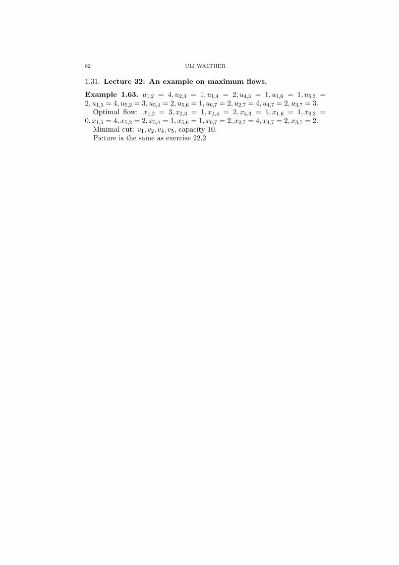
82 ULI WALTHER

1.31. Lecture 32: An example on maximum flows.

Example 1.63. u1,2 = 4, u2,3 = 1, u1,4 = 2, u4,3 = 1, u1,6 = 1, u6,3 =2, u1,5 = 4, u5,2 = 3, u5,4 = 2, u5,6 = 1, u6,7 = 2, u2,7 = 4, u4,7 = 2, u3,7 = 3.

Optimal flow: x1,2 = 3, x2,3 = 1, x1,4 = 2, x4,3 = 1, x1,6 = 1, x6,3 =0, x1,5 = 4, x5,2 = 2, x5,4 = 1, x5,6 = 1, x6,7 = 2, x2,7 = 4, x4,7 = 2, x3,7 = 2.

Minimal cut: v1, v2, v4, v5, capacity 10.Picture is the same as exercise 22.2

421 COURSE NOTES 83

1.32. Lecture 33: Applications of network simplex. This is, mostly,from chapter 20.

1.32.1. Inequality constraints in a network. What does one do in a networkproblem if the sources don’t have to be emptied but the sinks all need to befilled? (Under the assumption that the sources produces at least as muchas the sinks need.)

Answer: make up another node, the super-sink, and dreamroads that gofrom every source to the super-sink. Give them cost zero, and arrange thesuper-sink to have exactly the demand required to make demand and supplybalanced. Then use the old network simplex.

The same trick works of course for problems with more demand thansupply in which all supplies have to be taken care of. (Such an examplewould perhaps be the removal of garbage.)

1.32.2. Scheduling and inventory. Consider the following type of problem.A factory is supposed to export in the next 12 months dj amount of stuff,1 ≤ d ≤ 12. These numbers dj vary from month to month. They can makethe stuff in regular time, at cost a per unit, but they only can do that withr units per month (limits from the size of the plant). Or, they could makeit in overtime, at cost b per unit, but they can only make s units that wayper month. Whenever the production of one month exceeds the current dj ,the stuff goes into storage, which costs c per month and unit. Storage spaceis unlimited. If the numbers dj , r, s, a, b, c are known, how much should oneproduce how?

Answer: Make up a network as follows. Each month gets a node ofdemand dj . Each month also gets a node of supply r and a node of supplys. Finally, there is a node of demand equal to the supply of all other nodestogether (it’s the node representing all the stuff that was never made.)

Arcs are as follows. An arc from each s-node to its dj at cost b; an arcfrom each r-node to its dj at cost a; an arc from dj to dj+1 at cost c; anarc from each s-node and from each r-node to the strange node at cost zero.The arcs represent (in this order) overtime production in month j, regularproduction in month j, the amount of stuff in the warehouse in month j,the stuff never made in regular or overtime in month j.

A more involved problem is that of a caterer, see page 324.

1.32.3. Bipartite graphs. A graph is called bipartite or 2-colorable if one cancolor some of the vertices blue, and all others red, and no 2 vertices of thesame color are linked. This definition works both for directed and indirectedgraphs. (Directed means: arcs have directions.)

The idea of coloring is very old and was one of the inspiring questionsfor graph theory. It goes like this. Suppose you have a map (of somecountries), modeled just by a dot for each capital, and an arc between 2capitals if they share a border. Can one color all the vertices with 2 colorssuch that bordering countries have different color? The answer is rather

84 ULI WALTHER

obviously “no”, as one can see from a simple triangle. But if one asks thesame question for 3, or 4, or more colors, one might be prompted to thinkfor a while.

It turns out that 3 is not enough either, as is shown by the complete graphon 4 corners (complete refers to the fact that all vertices are linked to allothers). This graph can be pictured as a triangle with a dot in the middlelinked to all outer corners.

For 4 colors, the question has an interesting history. In the late 70’s,computer scientists Appel and Haken made a list of several thousand “little”maps that needed to be checked, and if these all could be done with 4colors then a mighty theorem said that then all maps (not just those testedexplicitly) could be 4-colored. Then they wrote a computer program to testthem. Unfortunately, all programs have bugs and so did theirs. So they keptfixing it. ALso, it turned out that the mighty theorem had some gaps. Atsome point the math community lost interest in their claims. Around 1990,with further improvements later, Robin Thomas at Georgia Tech vastlyimproved their method to reduce to around 100 basic graphs to check, anda correct mighty theorem. The underlying idea is based on flows of chargesin the graph, an idea due to Heesch in the 60s.

On the upside, 5-coloring is definitely true. There is an explicit algorithmthat shows how to color a map with 5 colors. No such algorithm is knownor really expected to exist for 4. Anyway, bipartite graphs are 2-colorableand these are the ones we will look at.

An interesting question is whether a graph is 1- or 2- or 3- or 4- colorable.1-colorable would mean, it represents a bunch of islands. 4-colorable is whatevery graph is expected to be. What about those in-between? Can we testa graph for its chromatic number, the least number of colored required tocolor the graph?

The question of testing for 2-colorability is easy. Take a vertex and makeit blue. All vertices adjacent to this must be red. Those adjacent to redvertices must again be blue and so on. Either this works, in which casethe graph is bipartite. Or, you run into a problem at some point. (Try to2-color the triangle!) Then the graph just isn’t. Testing for 3-coloring is alot harder, no efficient algorithms exist (but some inefficient ones).

Another thing that is interesting about bipartite graphs is making ofmatchings. A matching is a collection of disjoint pairs of red and bluevertices. For example, you can think of such a thing as a collection of dancingpairs out of a bunch of men and women where the arcs indicate acquaintance.Or for matchmaking where arcs indicate likely mutual interest.

Kind of an opposite thing is a cover. That is a collection of verticessuch that each arc of the graph involves at least one vertex of the cover.Obviously, each cover has at least as many points as any matching. This islike with the volume of a flow and the capacity of a cut. In fact,

421 COURSE NOTES 85

Theorem 1.64 (Konig-Egervary). In a bipartite graph, the size of thesmallest cover is equal to the size of the largest matching.

[Idea of proof: ] Interpret this as a cut-and-flow theorem. Figure 20.10indicates a network problem whose optimal solution points out the largestmatching in the graph. It has arcs from the blue to the red vertices. It isnow easy to find a cover of the same size as this matching: take all bluevertices with fair price 1 and all red ones with fair price zero. Clearly theoptimal schedule does not link 2 of these chosen vertices. Also, every arcthat is used from a blue to a red vertex is represented by one vertex. So thenumber is the same. 2

Note 1.65. In class, I did this slightly differently: you give each arc of Gcost -1, and all other arcs zero. Compute fair prices by putting the price atthe new corner next to the red vertices to zero. Then blue vertices can havefair price -1 or 0, while red vertices can have fair price 0 or 1. In this case,the cover consists of the red vertices of price 1 and the blue ones of price -1.

86 ULI WALTHER

Homework 12.

(1) 20.1. (Hint: usual simplex is not recommended.)(2) 20.8. (“Bottleneck” refers to the problem in which the quality of a

schedule is not determined by the sum of all used routes, but by theweakest link.)

421 COURSE NOTES 87

1.33. Lecture 34: More applications of the network simplex.

1.33.1. Assignment problems. Given 5 teachers and 5 courses, who shouldteach what? Suppose the following table gives the competence of eachteacher in all subjects.

Al 7 5 4 4 5Bob 7 9 7 9 4Charly 4 6 5 8 5Doreen 5 4 5 7 4Ellie 4 5 5 8 9

Many ways of “weighing” a schedule assignment exist: largest sum, largestminimum, largest maximum, etc.

Start with largest sum. Let xij indicate whether teacher i teaches coursej (with value 0 or 1). We therefore want to put binary values to these xi,jin such a way that there is exactly one xi,j nonzero in each column and ineach row. We want to maximize the sum of the competences. This calledan assignment problem.

Obviously, one can relax the condition “xi binary” to “xi ≥ 0” becausexi > 1 is clearly impossible (the sum of all xi,j in each row and column haveto add up to 1) and the network simplex finds integer optimal solutions tointeger network problems. Only question is: what is the appropriate networkproblem? Here it is:

n∑i=1

n∑j=1

(−si,j)xi,j → min

n∑i=1

xi,j = 1 for all j

n∑j=1

xi,j = 1 for all i

xi,j ≥ 0

Here, si,j is the competence of teacher i in subject j.Network simplex solves this. (Nodes are v1, . . . , vn, w1, . . . , wn, roads xi,j .

Each vi is a 1-source, each wj a 1-sink.)Note: we wrote ei,j for si,j in class.Note also: once we have seen transportation problems, we have a neater

way of dealing with these kinds of problems. The new way is, however, notmore efficient in an algorithmic way. It is just less writing for the samesteps.

1.33.2. What if we want to maximize the lowest score rather than the av-erage? (Weakest link tests.) First find some assignment. It will have somevalue V . Then one wants to see whether there are assignments with larger

88 ULI WALTHER

value t > V . To see if that can be done, erase from the transshipment prob-lem for the average optimization all arcs whose cost is not at least t. Solvethe modified problem. Iterate for increasing t. For t very large no arc is left,so at some point t is too big to give a solution for the modified problem.The largest t with a solution is the schedule maximizing the lowest score.

It seems to me that there is another way of doing the same problem in onestep. Namely, find the largest entry in the competence matrix (9 here) andcall it N . We mimic the Big-M method we met earlier. Then associate toarc xi,j cost MN−si,j . So all roads with competence N are assigned a 1, allroads of competence N −1 an M , all roads of competence N −2 an M2 andso on. In the same way as M is much larger than 1 we imagine M2 beingmuch larger than M etc. Solving the corresponding (minimizing) networkproblem gives a solution in which the largest exponent of M is minimized,which means that the largest difference between N and the efficiency anyused road is minimized, which means that the minimum efficiency used ismaximized. So that is exactly what we want.

421 COURSE NOTES 89

1.34. Lecture 35: Transportation problems. A transportation problemis of the form

n∑i=1

n∑j=1

ci,jxi,j → min

m∑i=1

xi,j = sj for all j

n∑j=1

xi,j = ri for all i

n∑i=1

sj =

m∑j=1

ri

sj , ri ≥ 0

xi,j ≥ 0

This is a transshipment problem with no intermediate nodes, all arcs gofrom sources to sinks and it’s called “balanced”.

Lemma 1.66. Every balanced transportation problem is feasible.

Proof. See homework. 2

In fact, balanced TP’s always have an optimal solution: we already knowthey are feasible, it is enough to remark that they are not unbounded. (Andthey aren’t because each arc xij is bounded by for example sj .)

How does one find a neat (that means, integral and tree) initial solution?(For the network simplex!)

1.34.1. Northwest corner rule. Pick x1,1 = min(r1, s1). Then either source1 or sink 1 is exhausted. Proceed dealing with the one that is not done yet.For example, if source 1 is exhausted, fill now sink 1 with source 2. Etc. Inthe matrix indicating the xi,j , this describes a path going from the upperleft (northwest) corner to the lower right.

We claim that this gives a tree for the simplex. Proof: A circuit wouldbe represented by a sequence of roads xi1,j1 , xi2,j2 , . . . , xin=i1,jn=j1 such thatfor all k either ik = ik+1 or jk = jk+1. In a solution for the NW rule, i andj never get smaller. So there can be no circuit.

Another way of seeing this is to note that if one cancels the arcs of theinitial solution in the order that the NW rule discovers them, then onealways cuts off a leaf from the initial solution. So there can’t be any circuit.

The NW corner rule is very simple to implement but unfortunately ignoresroad costs which might be bad in the long run.

90 ULI WALTHER

Example 1.67. The cost and demand data in

i\j 1 2 3 4 5 supply1 8 5 7 2 3 22 6 7 6 5 4 43 3 4 9 3 8 7

demand 3 2 4 2 2

give

i \ j 1 2 3 4 5 supply1 21 22 12 23 14 43 35 26 27 7

demand 3 2 4 2 2

with cost 16+6+14+6+27+6+16. The subscripts indicate in what orderwe found the loads. Draw the tree!

1.34.2. rising index method. Main idea is to give cheap roads large loads.

“Greedy method”

i \ j 1 2 3 4 5 supply1 21 02 22 26 25 43 33 24 27 7

demand 3 2 4 2 2

1.34.3. falling index method. Main idea is to give small loads to expensive

roads. “Conservative method”.

i\j 1 2 3 4 5 supply1 0 2 22 4 0 43 3 2 2 7

demand 3 2 4 2 2

Order

of determination: x3,3 = 0, x1,1 = 0, x3,5 = 0, so x3,2 = 2, x3,4 = 2, x3,1 = 3.Then x1,3 = 0, so x2,3 = 4, x1,5 = 2. One then fills in an appropriate numberof zeros to make the solution a tree. It is advantageous to use fields withsmall cost to place the zeros. This is the most tricky method.

Values of the three: 91,59,53. That is likely to be typical.There are other methods, for example Vogel-Korda approximation and

weighted frequency method which we don’t cover.Vogel: for all rows, all columns, find the difference (smallest) - (2nd small-

est). The pick row/column with largest such difference, and in that one thecolumn/row with the cheapest rout. Max out that road.

1.34.4. Testing for optimality. As in usual network simplex we try to findcircuits that promise improvement. 2 possibilities: either go back to drawinggraphs after the initial solution has been found. Or, do the whole thing inthe matrix. The latter is called potential method, and goes like this. Supposewe make up numbers ui and vj that signify the parts of the cost ci,j thatsource i and sink j pay for the transport of a unit along xi,j . Use the treeto determine these numbers assuming that u1 = 0. (There are one more ofthese cost charing variables than there are arcs in the tree, so we can setone of them as we want.)

421 COURSE NOTES 91

Now consider any road not in the tree. Suppose that ci,j < ui + vj . Thissignifies that combined source i and sink j would prefer to use that road.Putting loads on this road decreases and increases other roads in the circuitcompleted by xi,j and the tree. Shift as many loads as possible.

The tree is optimal if one cannot find any non-tree road with ci,j < ui+vj .The only purpose of the ui, vj is to find effectively those circuits that

bring improvement.Starting with the solution from the falling index method, we get u1 =

0, v4 = 2, v5 = 3, u2 = 1, u3 = 1, v1 = 2, v2 = 3, v3 = 5. Optimality followssince nowhere is the cost smaller than ui + vj .

Now start with NW solution. Then u1 = 0, v1 = 8, u2 = −2, v2 =9, v3 = 8, u3 = 1, v4 = 2, v5 = 7 and the most promising new arc isx3,1 (and x3,2). Increase load on x3,1 means to decrease on x2,1 and x3,3while increasing on x2,3. The best we can do is x3,1 = 1. New picture:

i\j 1 2 3 4 5 supply1 2 22 2 2 43 1 2 2 2 7

demand 3 2 4 2 2

Now u1 = 0, v1 = 8, u3 = −5, v3 =

14, v4 = 8, v5 = 13, u2 = −8, v2 = 15. Most promising roads are x1,2 and x1,5with 10/unit each. Let’s see which can be used more: both with 2. So, choosethe first. Then x1,1, x3,3, x2,2 go down by 2, and x1,2, x3,1, x3,2 go up by 2:

i\j 1 2 3 4 5 supply1 2 22 0 4 43 3 0 2 2 7

demand 3 2 4 2 2

Remember to leave some zeros to keep it

a tree. Now u1 = 0, v2 = 5, u2 = 2, v3 = 4, u3 = 5, v1 = −2, v4 = −2, v5 = 3.Best improvement is from x2,3 wit 6/unit. If x3,2 = t then we see that in-creasing is impossible, due to degeneration. The other promising road is x2,5with 1/unit. x2,5 = t gives x2,3 = 4− t, x3,5 = 2− t and x3,3 = t. The new

schedule is

i\j 1 2 3 4 5 supply1 2 22 0 2 2 43 3 2 2 7

demand 3 2 4 2 2

Now u1 = 0, v2 = 5, u2 =

2, v3 = 4, v5 = 2, u3 = 5, v1 = −2, v4 = −2. Now the only promising road isx3,2. We still can’t use it, but we must. The effect is a tree change without

a cost change. New solution:

i\j 1 2 3 4 5 supply1 2 22 2 2 43 3 0 2 2 7

demand 3 2 4 2 2

New po-

tentials are u1 = 0, v2 = 5, u3 = −1, v1 = 4, v3 = 10, v4 = 4, u2 = −4, v5 = 8.

92 ULI WALTHER

The best now is x1,5 with 5/unit. Making x1,5 large diminishes x1,2, x3,3 andx2,5 whence we take x1,5 = 2. This leads now to the solution that came outof the falling index and is optimal.

421 COURSE NOTES 93

Homework 13. (1) Prove that all balanced transport problems are fea-sible. (Hint: recall the proof of the wedding theorem.)

(2) Solve the following transport problem.1 2 3 4

1 1 7 6 8 42 7 25 13 20 63 6 14 9 15 54 1 30 13 16 2

3 7 3 4

94 ULI WALTHER

1.35. Lecture 36: An transport problem.

Example 1.68.

1 2 3 4 51 9 53 23 21 6 152 6 1 8 5 25 123 35 9 78 17 57 204 12 66 7 26 77 8

7 19 14 10 5Rising index method produces

1 2 3 4 51 7 3 5 152 12 123 7 3 10 204 8 8

7 19 14 10 5Falling index produces

1 2 3 4 51 7 3 5 152 6 6 123 19 1 204 8 8

7 19 14 10 5While NW produces

1 2 3 4 51 7 8 152 11 1 123 13 7 204 3 5 8

7 19 14 10 5The values are (I think) 671, 478 and 2109.

421 COURSE NOTES 95

1.36. Lecture 37: Transport example, second day. The optimal solu-tion is one step away from the falling index and is

1 2 3 4 51 7 3 5 152 3 9 123 19 1 204 8 8

7 19 14 10 5with value 475.

Note: Vogel-Korda is also one step from optimum. Note also that if oneuses “take the largest −(cij − ui− vj) and max it out”, cycling can happen.

96 ULI WALTHER

1.37. Lecture 38: Integer Programming. What is the smallest amountof coins needed to pay 49 cents? What if a nickel is worth 6 cents? Inprinciple, we know how to do this kind of problem: it really is a knapsackproblem kind of thing. (After some rewriting of the problem.) But, supposewe do perhaps want to answer this question not only for 49 cents, but for154 different other amounts of money. We would have to solve that manyknapsack problems. The point of what is to follow is to show that one cando one basic computation and 154 very easy ones instead.

Let c, n, d, q be the number of coins. Basically, we want to find valuesfor these numbers such that c + 5n + 10d + 25q = 49 and c + n + d + q →min. If this were a problem in which fractions are allowed, this wouldbe very easy to solve. The integrality condition is a major wrench in themachine however. These kinds of equations are called “Diophantine” afterDiophantus, who was a Greek mathematician and philosopher living about200-284. He investigated equations for their integral solutions. A famouscase is the “Fermat equation” xn + yn = zn for integer x, y, z. It has beenshown by Wiles and Taylor that this can only happen if

(1) z = 1 or(2) z = 0 or(3) n = 2.

That means, that the circle is the only of the Fermat curves with infinitelymany points with rational coordinates. All others have only 4 rational points(namely (±1, 0,±1) and (0,±1,±1)). This theorem made the front page ofthe NY Times, much to the surprise of the mathworld.

Another famous one is the Pell equation x2 − dy2 = ±1 where d is nota square. See http://bioinfo.math.rpi.edu/~zukerm/cgi-bin/dq.html

for a machine that finds solutions.Associate with the corresponding amount of money the monomial CcNnDdQq.

So 49 single cents mean C49. The point of using exponentials will becomeclear in a second. Imagine, if you will, that N stands for the procedureof paying a nickel, and multiplying these operations means execute themsuccessively.

Clearly, C49 corresponds to a feasible solution of our problem, but not toan optimal one. The cost function is the sum of the exponents. Large sumis bad, small is good.

We have replacement rules

(1) C5 = N ,(2) N2 = D,(3) N5 = Q.

The heavier of the two terms in each relation (with the larger exponentialsum) is called the leading term. Use them to make the input lighter::

C49 = C4N9 = C4ND4

421 COURSE NOTES 97

Now we are stuck although it is not likely that we have reached the optimum.⇒ there are relations between the coins that are somehow consequences, butnot obvious.

Fundamental trick: Take 2 relations, like the second and the third. AsN2 = D, N5 = N3D. As also N5 = Q, get rid of the heaviest term in bothto obtain a “lighter relation” N3D = Q. The left can be made even lighter:since N3D = ND2, then ND2 = Q. Make this relation (4).

Then C47 = C2ND4 = C2D2Q. This is probably optimal, but can we besure? (Note: the main reason that we think it is optimal is because it is the“greedy” solution to the problem: first pay as many quarters as possible,then as many dimes, then as many nickels, and take the rest pennies. Thepoint is that we have seen before that greedy algorithms don’t usually giveoptimal solutions.)

Maybe there are more useful relations hidden? Actually, there are. Be-cause if someone came along with three dimes, we would not know how turnthem into fewer coins, except by clever thinking. Clever thinking is bad,because in real life it is too hard. Hence, we make an algorithm that alwaysfinds all relations: It is an abstraction of the method by which we foundrelation 4 above.

98 ULI WALTHER

1.38. Lectures 39, 40: Grobner bases and Buchberger algorithm.

1.38.1. Generalization: What if we had to answer the pennies question, butwhere the coins have weights p → 1, n → 3, d → 2, q → 7 and we want tominimize the total weight?

What are the other possibilities for ordering?

Definition 1.69. A monomial ordering in a ring of polynomials R[x1, . . . , xn]is a way of comparing monomials such that

(1) 1 ≺ m for every monomial,(2) if m ≺ m′ then mm′′ ≺ m′m′′ for all monomials m,m′m,′′.

Here are some examples.

Example 1.70. (1) lex: adopt the alphabet in which x1 is the firstletter, x2 the second, and so on. Lex then considers monomials aswords in which the earliest letters are written first and comparesthem like in a dictionary. So,

x1x2x3 ≺ x1x2x2 ≺ x1x1 ≺ x1x1x1because in a dictionary with alphabet x1, x2, x3 the word x1x1 wouldbe the first and x1x2x3 the last of the three. As was pointed outto me, the analogy is not quite perfect: x1x2 for example is biggerthan x1 although ab would come after a in most dictionaries. Thus,lex orders by alphabet with the caveat that if one word is containedin the other, the bigger comes first. (Another way of saying that is,that any letter comes before the “not-letter” in the alphabet.)

(2) deglex=grlex: First compare two monomials by their degree, andif that is equal then use lex. So

x1x1 ≺ x1x2x3 ≺ x1x2x2in deglex.

(3) weight orders: let w = (w1, . . . , wn). Compare two monomials bytheir weight. Note: this may lead to ties between monomials.

(4) total weight orders: like weight orders, but if 2 monomials are tiedby weight, compare them by lex.

(5) degrevlex: First compare two monomials by degree. If that is equal,prefer the one that has fewer xn-factors. If that is equal, take the onewith fewer xn−1-factors. Etc. Note: this is a bit like deglex upsidedown, but is not simply the opposite of deglex. For example,

x1x3x3 ≺ x1x2x3 ≺ x2x2x2in degrevlex while

x2x2x2 ≺ x1x3x3 ≺ x1x2x3in deglex. So some relations are the same and some turn around.

If confusion is possible, one puts a subscript on the ≺ to indicate whatorder one is talking about.

421 COURSE NOTES 99

Definition 1.71. With a monomial order one can define the initial term ofa polynomial p, it is the largest term in p under the particular order. Wewrite in≺(p).

So for example, under deglex, in(c5 − n) = c5.

Definition 1.72. The ideal to a bunch of relations is the entire collectionof all possible consequences of the relations. So if the given relations arec5 − n and n2 − d then for example n(c5 − n) − 1(n2 − d) = nc5 − d is oneelement of the ideal. So is 3(c5 − n)− c2 ∗ n(n2 − d) and all other possible(sort of) linear combinations of the two given relations.

Return to w = (1, 3, 2, 7). A GB for the money ideal is given by

c5 − n, n2 − d, q − nd2

is a GB if nd2 ≺ q. (Note the tie!) If q ≺ nd2, the GB is

c5 − n, n2 − d, nd2 − q, nq − d3, q2 − d5.So little changes in the order can have great effects in the GB.Algorithm 1.73 (Buchberger).Input: A collection of binomials (the exchange rules that are known). Atotal monomial order.Output: A collection of binomials by means of which every “minimal num-ber of coins” problem can be solved.

(1) Write each binomial as “heavier term - lighter term”.(2) Pick a pair of binomials that has not been picked before. Multiply

each by a suitable monomial such that their heavier terms becomeequal. Subtract to cancel the two heavier terms.

(3) Using all known relations, make each term of the difference as lightas possible.

(4) If the result is 0 = 0, mark the pair we just did as “done” and startover.

(5) If the result is nonzero, add the new relation to the known ones,mark the pair we just used as “done” and start over.

(6) Stop when all pairs are marked “done”, and output all relationsknown at that point.

The magic is:

Theorem 1.74. The algorithm will stop. The output solves for each amountof money given in any possible way the question “how do you minimize thenumber of coins for this amount of money” by mindless reduction. This“complete” collection of exchange rules is a “Grobner basis”.

100 ULI WALTHER

1.39. Lecture 41: Grobner bases with Maple.

Example 1.75. What is the least weight of coins needed to pay 49 cents?A Grobner basis can be computed, for example, by Maple:

with(Ore_algebra);

with(Groebner);

A := poly_algebra(C,N,D,Q);

T := termorder(A,tdeg(C,N,D,Q));

E := [C^5-N,N^2-D,N^5-Q];

G := gbasis(E,T);

normalf(C^(49),G,T);

In our example, the output is N2−D,D3−N,ND2−Q,C5−N . Moreover,C4D2Q is indeed the best way of paying 49 cents.

One can find out more about the termorders by help(termorder);. Iffor example one would like to know all the relations between c, n, d, q thatdon’t use d, one writes

B := poly_algebra(C,N,D,Q);

TB := termorder(B,plex(D,D,N,Q));

EB := [C^5-N,N^2-D,N^5-Q];

GB := gbasis(EB,TB);

The output Q − C25, C − N5, D − C10 indicates that the only relationsbetween Q,C,N are the first two. There is a theorem that says if one useslex then the relations in a GB not involving the first variable generate allrelations between just the other variables.

Now let’s look at what happens if a nickel is 6 cents, but we still want topay 49 cents. The “natural” approach is to say, well first take a quarter andsee what is left (49-25=24). Then use the next largest coin to subtract 20cents as 2 dimes. Then 4 cents are left, and that means we need 4+2+1=7coins. Apparently, the change of value for the nickel makes in this caseno difference. Let’s ask Maple though, to be safe. Of course, our inputequalities change, so we express everything in cents rather than nickels:

E2 := [C^6-N,C^(10)-D,C^(25)-Q];

G2 := gbasis(E,T);

421 COURSE NOTES 101

Now the Grobner basis is quite tremendous:

ND2 − CQC2D −N2

CD3 −NQN3D − C3Q

D5 −Q2

N5 −D3

CN4 −QC2N3 −D2

C4N −DC3N2Q−D4

C5Q−D3

C6 −NSome strange things happened, for example the existence of exchange rela-tions with equal weights on both sides. The real hit though is

normalf(C^(49),G2,T);

resulting in N4Q, which are only 5 coins.

102 ULI WALTHER

Uses of GB:

• lex gives elimination ideals.• initial ideals are deformations.• test whether g is a consequence of f1, . . . , fk.

Morals: Greedy behavior may not be optimal. Grobner bases are all-knowing,but may be large. They can be computed with Maple.

421 COURSE NOTES 103

Homework 14. (1) In the ring of polynomials R[x, y, z], order the fol-lowing monomials• by lex• by grlex• by the weight order w = (3, 4, 5) which breaks ties according to

lex1, x, y, z, x2, xy, y2, xz, z2, yz.

(2) Prove that

{x− y2w, y − zw, z − w3, w3 − w}form a Grobner basis with respect to lex where the order of letters inthe alphabet is x > y > z > w. Prove that these same polynomialsare not a Grobner basis with respect to lex if the alphabet readsw > x > y > z.

104 ULI WALTHER

1.40. Lectures 42, 43, 44: Review of final material, questions.

421 COURSE NOTES 105

final material

• determine value, optimal strategy, fairness of a game• network simplex: finding initial solution, network simplex algorithm• upper bounded transshipment problems: initial solution, algorithm• network flow algorithm: minimal cuts/maximal flows, Ford/Fulkerson• covers and matchings in bipartite graphs• assignment problems: best sum, and bottleneck version• transport problems: NW corner rule, rising index, potential method• Grobner bases: test a collection of relation whether they are a GB

Purdue UniversityE-mail address: walther@math.purdue.edu