Contents — T - lpi.usra.edu · MGS TES data over the poles are taken much more frequently than...

Contents — T

Water Cycling in the North Polar Region of Mars L. K. Tamppari, M. D. Smith, A. S. Hale, and D. S. Bass....................................................................... 3121

Mars: Updating Geologic Mapping Approaches and the Formal Stratigraphic Scheme K. L. Tanaka and J. A. Skinner Jr. ......................................................................................................... 3129

Igneous and Aqueous Processes on Mars: Evidence from Measurements of K and Th by the Mars Odyssey Gamma Ray Spectrometer

G. J. Taylor, W. Boynton, D. Hamara, K. Kerry, D. Janes, J. Keller, W. Feldman, T. Prettyman, R. Reedy, J. Brückner, H. Wänke, L. Evans, R. Starr, S. Squyres, S. Karunatillake, O. Gasnault, and the Odyssey GRS Team.................................................................................................................... 3207

The Microscope for the Beagle 2 Lander on ESA’s Mars Express N. Thomas, S. F. Hviid, H. U. Keller, W. J. Markiewicz, T. Blümchen, A. T. Basilevsky, P. H. Smith, R. Tanner, C. Oquest, R. Reynolds, J.-L. Josset, S. Beauvivre, B. Hofmann, P. Rüffer, C. T. Pillinger, M. R. Sims, D. Pullan, and S. Whitehead ...................................................... 3015

The South Polar Residual Cap of Mars: Landforms and Stratigraphy P. C. Thomas .......................................................................................................................................... 3058

Carbonates on Mars: Probable Occurrences, Spectral Signatures, and Exploration Strategies B. J. Thomson and P. H. Schultz ............................................................................................................ 3229

Great Martian Dust Storm Precursor? J. E. Tillman ........................................................................................................................................... 3164

Temporal and Spatial Distribution of Seasonal CO2 Snow and Ice T. N. Titus and H. H. Kieffer .................................................................................................................. 3273

Correlation of Neutron-sensed Water Ice Margins with Topography Statistics R. L. Tokar, M. A. Kreslavsky, J. W. Head III, W. C. Feldman, K. R. Moore, and T. H. Prettyman ............................................................................................................................... 3181

Low-Temperature Aqueous Alteration on Mars: Insights from the Laboratory N. J. Tosca, S. M. McLennan, D. H. Lindsley, and M. A. A. Schoonen .................................................. 3178

The Beagle 2 Environmental Sensors: Intended Measurements and Scientific Goals M. C. Towner, T. J. Ringrose, M. R. Patel, D. Pullan, M. R. Sims, S. Haapanala, A.-M. Harri, J. Polkko, C. F. Wilson, and J. C. Zarnecki ...................................................................... 3024

Convective Plumes as ‘Columns of Life’ B. J. Travis ............................................................................................................................................. 3230

Sixth International Conference on Mars (2003) alpha_t.pdf

WATER CYCLING IN THE NORTH POLAR REGION OF MARS. L. K. Tamppari1, M. D. Smith2, A. S. Hale3, and D. S. Bass3, 1NASA Jet Propulsion Laboratory (4800 Oak Grove Drive, Pasadena, CA 91109 [email protected]), 2NASA Goddard Space Flight Center ([email protected]), 3NASA Jet Propulsion Laboratory (MS 264-235, 4800 Oak Grove Drive, Pasadena, CA 91109 [email protected]), 4NASA Jet Propulsion Laboratory (MS T1722, 4800 Oak Grove Drive, Pasadena, CA 91109 [email protected]).

Introduction: The Martian water cycle is one of the

three annual cycles on Mars, dust and CO2 being the other two. Despite the fact that detailed spacecraft data, including global and annual coverage in a variety of wavelengths, have been taken of Mars spanning more than 25 years, there are many outstanding ques-tions regarding the water cycle.

There is very little exposed water on Mars today, in either the atmosphere or on the surface [1] although there is geological evidence of catastrophic flooding and continuously running water in past epochs in Mars' history [2] as well as recent (within about 10,000 years ago) evidence for running water in the form of gullies [3]. While there is little water in the atmosphere, wa-ter-ice clouds do form and produce seasonal clouds caused by general circulation and by storms [5-8]. These clouds may in turn be controlling the cycling of the water within the general circulation [e.g., 6].

The north polar cap region is of special interest as the residual cap is the main known reservoir of water on the planet today. The south polar residual cap may contain water, but presents a CO2 ice covering, even during southern summer. This hemispheric dichotomy is unexplained and is especially puzzling due to the fact that the Martian southern summer is much warmer (due to Mars' eccentricity) than the northern summer. Re-cently, water has been found in the top meter of the surface in both the northern and southern high latitude regions [e.g. 8-9] indicating an even greater amount of water on Mars than previously known.

Background: In order to better understand the cur-rent climate of Mars, we seek to understand atmos-pheric water in the north polar region. Our approach is to examine the water transport and cycling issues within the north polar region and in/out of the region on seasonal and annual timescales. Viking Mars At-mospheric Water Detector (MAWD) data showed that water vapor increased as the northern summer season progressed and temperatures increased, and that vapor appeared to be transported southward [10]. However, there has been uncertainty about the amount of water cycling in and out of the north polar region, as evi-denced by residual polar cap visible brightness changes between one Martian year (Mariner 9 data) and a sub-sequent year (Viking data). These changes were origi-nally thought to be interannual variations in the amount

of frost sublimed based on global dust storm activity [10-12]. However, Viking thermal and imaging data were re-examined and it was found that 14-35 pr �m of water -ice appeared to be deposited on the cap later in the summer season [14], indicating that some water may be retained and redistributed within the polar cap region. This late summer deposition could be due to adsorption directly onto the cap surface or due to snowfall. The possibility that some of the water is sea-sonally sequestered in water-ice clouds and may allow later precipitation had not been previously considered. We address these issues by examining water vapor and water-ice clouds in the north polar region of Mars dur-ing the north spring and summer period.

Method: Water-ice clouds. Water-ice clouds, in the north

polar region, have previously been tentatively identi-fied in the Viking era using the Infrared Thermal Map-per (IRTM) data [14] and in the Mars Global Surveyor (MGS) era using the Thermal Emission Spectrometer (TES) data ([15] and M. Smith, pers. comm., 2001). The Viking data provides only nadir pointed data, which necessitates separating the surface contribution from the atmospheric contribution. The technique used relies on the water-ice absorption feature at 11-microns. Specifically, it uses the 11- and 20-micron channels of the IRTM instrument along with a surface model to accurately remove the surface contribution [4]. For the Viking time frame, we are restricted to ice free surfaces and therefore do not see the entire north polar cap region throughout the spring and summer season.

With the MGS TES data, there exist both limb- and nadir-pointed data. The nadir-pointed data retriev-als are currently performed for water ice clouds only over surfaces above 220 K (M. Smith, pers. comm.). The surface is colder than 220 K northward of 60° N at Ls=0°, but this latitude limit moves gradually north-ward as spring progresses, reaching the pole just before Ls=90°. The TES limb data do not have any compli-cations due to cold surface temperatures. Therefore, water-ice clouds can be identified throughout the Mar-tian season, even over the seasonal and residual polar cap.

Sixth International Conference on Mars (2003) 3121.pdf

MGS TES data over the poles are taken much more frequently than over other areas of the planet due to the nature of the orbit. The nominal TES observing sequence has limb-geometry observations taken every 10 degrees in latitude. The orbit of MGS is such that over a 2-sol period (approximately 1 degree of Ls), approximately 24 orbits of Mars are made with tracks spaced roughly evenly every 15 degrees in longitude. Therefore, in the polar region, while not as dense as the nadir-geometry observations, the limb-geometry obser-vations help to fill out the data set and provide an addi-tional cut through the atmosphere from which to iden-tify clouds and vapor. The limb data also offer the possibility to detect the cloud heights as there are mul-tiple spectra over the vertical range.

Water vapor. Smith et al. [17] have performed re-trievals for the column-integrated abundance of water vapor using the rotational water vapor bands at 220-360 cm-1. Atmospheric temperatures are first retrieved using the 15-�m CO2 band (Conrath et al., 2000). Next, a forward radiative transfer computation is used to find the column-integrated water abundance that best fits the observed water vapor bands. At this time water is assumed to be well-mixed up to the condensation level and then zero above that. A total of six water vapor bands between 220 and 360 cm-1 are observed in TES spectra and the widths and relative depths of all six bands are very well fit by the synthetic spectra. Because the spectral signature of water vapor is spec-trally very distinct from those of dust and water-ice, we can easily separate the relative contributions from each component (dust, water-ice, and water vapor) on a spectrum-by-spectrum basis.

Recent analysis with MGS TES data has shown evidence for water vapor "pulses" as the seasonal north polar cap sublimes [15]. This could be linked to the previous late-summer season deposition, discussed above. Additionally, there may be some differences in the details of the water vapor as a function of latitude and season between the Viking era and the current era. Any such differences would help identify and charac-terize the degree of interannual variability in the water vapor. There is also indication of latitudinal water vapor transport as a function of season seen through longitudinally averaged water vapor [16 and Figure 1]. We will present our latest results on water vapor trans-port, spatially and temporally.

Figure 1. Longitudinally averaged water vapor as

a function of latitude for Ls=115° (top) and Ls=117° (bottom). The amount of water vapor in the centermost ring (highest latitude ring) shows about a 15 pr micron enhancement in 2° Ls, while the 3rd and 4th rings from the center show a decrease in vapor amount.

Dust. Dust in the north polar region can play an

important role in the water cycling story in a couple of ways. One, by acting as cloud condensation nuclei, dust may allow water-ice clouds to form and could potentially cause gravitational settling and sequestering of the water. Two, dust may be sufficiently radiatively active to prohibit clouds from forming and potentially allowing a greater degree of water vapor transport out of the polar region. The MGS TES instrument also spans the wavelength region over which Martian dust is absorbing, allowing its retrieval.

Surface Temperature. The north polar region sur-face temperature during the northern polar season can be compared to the Viking era to further elucidate po-tential interannual differences and to understand the vapor, water-ice, and dust retrievals. MGS TES is also


capable of measuring the surface temperature. Surface temperatures can confirm that carbon dioxide is not present on the cap surface, implying that any brighten-ing is likely water ice.

Intercorrelation of data: To date, there has been no comprehensive study to understand the partitioning of water into vapor and ice clouds, and the associated effects of dust and surface temperature in the north polar region. Ascertaining the degree to which water is transported out of the cap region versus within the cap region will give much needed insight into the overall story of water cycling on a seasonal basis. In particu-lar, understanding the mechanism for the polar cap surface albedo changes would go along way in com-prehending the sources and sinks of water in the north-ern polar region. We approach this problem by exam-ining TES atmospheric and surface data acquired in the northern summer season and comparing it to Viking data when possible. Because the TES instrument spans the absorption bands of water vapor, water ice, dust, and measures surface temperature, all three aerosols and surface temperature can be retrieved simultane-ously. This presentation will show our latest results on the water vapor, water-ice clouds seasonal and spatial distributions, as well as surface temperatures and dust distribution which may lend insight into where the wa-ter is going.

References: [1] Keiffer H. H. et al. (1976) Science, 194, 1341-1344 [2] Carr, M. H. (1998) Water on Mars [3] Malin M. C. and Edgett, K. S. (2001) JGR 106, 23429-23570. [4] Tamppari, L. K. et al. (2000) JGR 105, 4087-4107. [5] Smith, M. D et al. (2001) JGR 107, 5115-5134. [6] Richardson, M. I. et al. (2002) JGR 107, 5064-5093. [7] Hollingsworth, J. L. et al. (1997), Nature 380, 413-416. [8] Feldman W. C. et al., (2002) Science 297, 75-78 [9] Boynton W. V. et al., (2002) Science 297, 81-85 [10] Jakosky, B. M. (1985), Space Sci. Rev. 41, 131-200. [11] James P. B. and Martin L. (1985) Bull. Amer. Astron. Soc., 17, 735. [12] Kieffer H H. (1990) JGR, 96, 1481-1493. [13] Bass D. S. et al. (2000) Icarus, 144, 382-396. [14] Tamppari L. K. and Bass D. S. (2000) 2nd Mars Polar Conf. [15] Tamppari L. K. et al. (2002) Bull. 34th Am. Astron. Soc., 845. [16] Tamppari L. K. et al. (2003) LPSC XXXIV, Abstract #1650. [17] Smith M. D. et al. (2000), Bull. AAS, 32(3), 1094.


MARS: UPDATING GEOLOGIC MAPPING APPROACHES AND THE FORMAL STRATIGRAPHICSCHEME. K. L. Tanaka and J. A. Skinner, Jr., U.S Geological Survey, 2255 N. Gemini Dr., Flagstaff, AZ 86001;[email protected].

Introduction: At the Fourth Mars Conference in1989, Tanaka reviewed the stratigraphy and geologichistory of Mars that had emerged based on systematicgeologic mapping of the planet’s surface using Vikingdata [1]. This review looked at the stratigraphic col-umn for Mars and assessed the global geologic historyin terms of impact, fluvial, periglacial, aeolian, vol-canic, and tectonic processes. Many significant newstudies using Mars Global Surveyor (MGS) and nowMars Odyssey (MO) data are showing some importantnew insights and discoveries that are altering anddeepening previous understandings. If we were to il-lustrate the current state of the science, we might com-pare it to a loose-leaf notebook in which pages arerapidly being added, removed, and rewritten, withplenty of room remaining. Much of the flux is due tonew data, of course, but also much can be attributed tothe re-examination of basic assumptions and ap-proaches and our ability to employ ever more powerfulcomputer techniques. Here, we will attempt to review,based on our experience, the areas where the mostchange seems to be occurring, what prospects we facein the immediate future, and where caution needs to beexercised.

Geologic Mapping Approaches: The fundamentaltechnique for reconstructing the history of planetarysurfaces is geologic mapping. Maps portray the distri-bution of rock units and surface features as they devel-oped through time, based on morphologic relative-ageindicators including superposition and cross-cuttingrelations as well as crater-density determinationswhere possible, as on Mars.

Previous Methods and Their Shortcomings. Gener-ally, map units for Mars have been based on morphol-ogy, albedo, relative ages, and topography using Mari-ner 9 and Viking images. These data have proved to bevaluable but challenging to map with, because of in-consistencies in or problems with resolution, atmos-pheric opacity, solar illumination, and image locating.MGS MOLA data have been extremely valuable inproviding improved topographic and morphologicviews over much of the planet’s surface. However,cross-track spacing is locally quite large in the equato-rial region and above 87° latitudes, where off-nadirpointing was required. New, largely nadir visible andthermal infrared images of the surface by MGS MOCand MO THEMIS provide higher resolution and dif-ferent wavelength views of the surface. MOC NA im-ages reveal close-up views of morphology and albedo

features at meters to tens of meters scales such as rocklayers and craters [2]. Depending on scale, these newdata sets will likely justify revised mapping of Mars.

While the prospects for new results detailing thegeologic history of Mars are bright based on new dataalone, improved mapping methods will also be signifi-cant. Since the days of systematic geologic mappingusing Mariner 9 data, Mars geologic map units havebeen characterized and named on the basis of mor-phologic and albedo features that we now (as well aspreviously) realize represent secondary features relatedto surface modification and tectonic deformation(rather than to the primary origin of the unit). Exam-ples of secondary descriptors in unit names include“ridged,” “lineated,” “channel,” “dissected,”“cratered,” “mottled,” “etched,” “knobby,” “smooth,”and “rough.” Albedo seems to be a consistently map-pable characteristic only where the surface is free fromdust due to recent atmospheric activity; (e.g., polarresidual ice, which varies annually in extent), or wherethe dust and soil themselves are being mapped. How-ever, much of the planet is covered by a shifting man-tle of dust as indicated by high albedo and low thermalinertia data.

Some units have composite signatures of signifi-cance, but the unit name may focus on only one item.Thus, “knobby material” usually signifies knobs of onematerial surrounded by plains-forming material of an-other material type and age. Finally, unit descriptorterms usually have relative and thus imprecise mean-ing; as an example, a “smooth” surface at small scalemay be characterized as “rough” at larger scales. Thusmorphology, albedo, and other surficial data must beused with caution, if at all, in defining map units. Inmany cases, it may be difficult to determine whetherparticular signatures are primary or secondary (e.g., thehigh albedo of a rough surface could be primary or itmay represent a coating of much younger, high-albedoaeolian material).

The use of secondary features in unit names anddefinitions engenders the misconception that the sec-ondary features are either primary or at least about thesame age as the material unit being mapped. Evenworse, mappers may be inclined to map material unitcontacts on the basis of the presence or absence ofthose features without carefully testing this approach.These issues have been addressed in the case of photo-geologic mapping of planetary surfaces marked bytectonic structures [3], which is particularly applicable


MARS: GEOLOGIC MAPPING APPROACHES: Tanaka K. L. and Skinner, J.A., Jr.

to Venus and outer planet satellites. The Moon, Mer-cury and Mars also have surfaces displaying sufficientranges in crater densities to provide an effective tool inrelative-age dating. Mars is an especially complexcase, because it also has experienced significant ero-sion. Thus determining the relative ages of secondaryfeatures requires special care. For example, featureterminations (e.g., of grabens or valleys) may representeither the original, full extent of the features or theextent to where obliteration has occurred due to resur-facing by erosion, degradation, or burial by youngermaterial. To discriminate between these possibilities,additional evidence is required such as embayment byyounger material. It is insufficient to rely solely on alower crater density where the features are missing,because erosion or the former presence of mantles mayaccount for a lower crater density and not youngermaterial.

While it may be particularly evident that manymorphologic and albedo signatures may be secondaryand thus should not be included in map-unit definitionsand names, we also see a danger in using terrain de-scriptors, such as “highlands,” “plains,” “hilly,”“floor,” and “basement.” Such descriptors force themapper to pigeonhole outcrops on the basis of terrain,although geologic units may actually occur in multipleterrain settings. Furthermore, terrain descriptors do notmake sense in cross section, as in “ridged plains mate-rial” that may make up kilometers-thick sequences offlows exposed in the walls of Valles Marineris andKasei Valles or as in “channel floor material” actuallymade up of scoured older material. In some cases, butnot generally, mappers have called these units “geo-morphic units,” recognizing they represent youngersurfaces rather than younger materials. However, suchmaps suffer from the added complexity of not beingfully geologic maps.

Another shortcoming in much of the previous geo-logic mapping of Mars has been the nature of contactrelations among map units, which was not studiedcarefully, not documented adequately, and/or notmapped in detail using multiple contact types. Thus thereader is left uninformed about the specific inferencesand their associated uncertainties used in defining mapunits, in mapping contacts, and in determining relative-age relations between units. Many contacts amongNoachian materials and younger plains-forming mate-rials in particular have been described as gradational,which could mean gradational in morphology, age,lithology, provenance, emplacement processes, etc.,with adjacent units.

Improved Mapping Approaches. We are imple-menting some significant new approaches in our geo-logic map of the northern plains of Mars (in progress)

in order to overcome the aforementioned shortcom-ings. These approaches may need further refinementand thus should be regarded as tentative.

First, we are not using morphology, albedo, terrain,or any other physical characteristics in map-unitnames. Following terrestrial methods, units are namedstrictly after associated geographic terms (e.g., VastitasBorealis Formation). They may also be distinguishedby geochronologic period (e.g., Noachian), relativestratigraphic position (e.g., upper, lower, 1, 2, 3),and/or lateral facies (interior, exterior, marginal,proximal, distal).

Second, we define map units only by their apparentprimary features, and secondary features are discussedonly as they relate to unit character. Examples of thelatter include inferences such as yardangs indicative offriable materials and steep scarps suggestive of resis-tant material. In addition to lithologic (rock-stratigraphic units), we recommend also mappingunconformity-bounded units (UBUs) [4] (or allostrati-graphic units [5]) that discriminate material units byrelative age, wherever a significant hiatus can be dem-onstrated in the geologic record. Also, these units mayconsist of multiple lithologies, useful when an intimatemixture of diverse lithologies may prove to be imprac-tical to map but all have a geologic and temporal asso-ciation. Thus lobate materials of diverse, mixed mor-phologies in Utopia Planitia may include lava and ashflows, lahars, and mudflows of diverse lithology but allrelated to the same period of volcanism and erosion ofthe western flank of the Elysium rise as defined bystratigraphic relations and crater counts. Another ex-ample would be two sets of overlapping lava flows inwhich the older set is faulted by grabens and theyounger set buries the grabens. While UBUs have beenused in essence in previous mapping to some degree,the lack of their formal recognition as a legitimate unittype has resulted in inconsistency in their application.

Third, we avoid discriminating units having con-siderable overlap in both character and age. We thushave not separated out both Late and Middle Noachianhighland units in our northern plains mapping (as inthe cratered and subdued units of the plateau sequenceas mapped previously [6]). Most Noachian surfacesshow high variability in crater densities and terrainruggedness, but few display strong morphologic indi-cations of embayment and overlap relations that relateto distinctive epochs. We only have mapped within~300 km of the highland/dichotomy boundary; andLate Noachian materials appear to occur elsewhere,such as material covering Thaumasia Planum south ofCoprates Chasma [7].

Fourth, we attempt to lump or split units based ongeologic associations at map scale. This is not a new



approach, but implementing it has improved now thatMOLA and other new data better define topographicand other associations for provenance of deposits andsource regions of volcanic flows.

Fifth, we more carefully define and map contacttypes according to USGS standards [8], including:certain, approximate, gradational, inferred, and in-ferred approximate.However, the USGS guidelinesseem to be poorly defined, so we have provided ourown: Certain denotes a precise contact between well-characterized material units, whereas approximatecontacts are less precisely mapped due to data quality,subtlety of the contact, and/or secondary surface modi-fication. Gradational contacts are used around com-posite units made up of intimate mixtures (at mapscale) of older materials and their apparent erosionalproducts, such as knobs of older material surroundedby younger slope material; such units grade with adja-cent, continuous outcrops of both the older materialand younger plains-forming material at the base of theknobs. Inferred contacts are used when the materialdistinctiveness between the map units is subject toquestion. An example is the contact between what weare mapping as the interior and marginal members ofthe Vastitas Borealis Formation. The interior membermay be simply a different morphologic expression ofthe same material and emplacement age as the mar-ginal member, or it may represent material of the mar-ginal member that was later pervasively and intenselyreworked. Digital mapping of line work greatly facili-tates the drafting and editing of multiple contact types.

The Formal Martian Stratigraphic Scheme:Surprisingly, the scheme initially introduced by Scottand Carr [9] from Mariner 9 based global geologicmapping and later refined using Viking global geologicmapping results and crater-density data [1], has fairlywell withstood the test of time and dozens of local andregional studies in the assigning of relative-ages basedon crater densities and stratigraphic relations. How-ever, aspects of the scheme are either flawed or needrevisiting.

Referents and Time-Stratigraphic Units. The pre-sent stratigraphic scheme for Mars is based on the for-mal time-stratigraphic methodology developed forEarth [5]. Time-stratigraphic (or chronostratigraphic)units define stratigraphic position and are based onrock units that can be used to define a specific periodof geologic time; the base of the unit represents thebeginning of the period. Time-stratigraphic units formSystems and their subdivisions, Series, and their chro-nologic equivalents are Periods and Epochs. Thusheavily cratered material in Noachis Terra defines theNoachian System position and the Noachian Periodage category, and intercratered plains material defines

the Upper Noachian Series, corresponding to the LateHesperian Epoch [1].

Increasingly, it is apparent that using material ref-erents to define the spans of time-stratigraphic units onMars does not work well, because of many uncertain-ties in the temporal character of the geologic units andthe lack of temporal continuity among the referents.Also, photogeologic techniques necessarily limit theinspection of material units to surface exposure, and solittle is known about their vertical character. Thusstratigraphic columns remain poorly defined. Some ofthe specific problems include: (1) The base of theLower Noachian basement material is unexposed andthus remains stratigraphically undefined. (2) MiddleNoachian cratered terrain and Upper Noachian inter-crater plains materials are intergradational with eachother as well as with older and younger units. Thismeans that the ages of parts of the units fall outside thetime-stratigraphic positions and periods they are meantto define. Also, the end of the Noachian is commonlyviewed as when widespread valley formation and cra-ter degradation largely ceased on Mars. However,some evidence indicates that that cessation may betime transgressive and controlled by elevation [10]. (3)Lower Hesperian ridged plains material is mapped inmany areas across the planet, but some patches actu-ally have Late Noachian crater densities [7]. Also,wrinkle ridges deform plains materials in caldera floorsand northern plains surfaces, which reminds us thatwrinkle ridges are not primary features and thus do notnecessarily relate temporally to the materials they de-form. Finally, MGS and MO data are revealing thatHesperian Planum itself may be complex stratigraphi-cally. (4) Upper Hesperian complex plains material,representing the Vastitas Borealis Formation likelyconsists of sedimentary material related to inundationof the northern plains. The unit may represent a verybrief moment in geologic time, rather than a truly ex-pansive epoch. (5) The Lower and Middle Amazonianreferents are deposits and lobate materials whose de-tailed histories remain to be determined. (6) The UpperAmazonian flood-plain material in Elysium Planitianow appears to be largely flood lavas that were em-placed in an extremely young and brief event.

Crater-Density Definitions and Precautions. Ta-naka [1] used the type material referents to help deter-mine the crater-density boundaries to the time-stratigraphic units, which has been a very useful appli-cation of that stratigraphic scheme. However, forstratigraphic applications, crater-density relative-agedeterminations have some serious limitations that needto be kept in mind. Crater densities provide, assumingno subsequent resurfacing, a mean surface age. Thus,unexposed, older parts of the unit cannot be accurately



dated, although in some cases the crater age of buriedsurfaces can be inferred by the density distribution oflarge, partly buried craters and depressions indicatingpossible buried craters. In addition, map units mayinclude outcrops of greatly varying age, in which thecrater sample size of individual outcrops may be insuf-ficient to effectively constrain age. Thus, the standarddeviation of the mean crater age may be a rathermeaningless quantity when it comes to defining theage range of units. An extreme example would be aHesperian crater density resulting from a map unit thatincludes individual outcrops of Noachian, Hesperian,and Amazonian material.

Another problem that is increasingly noted is theeffects of resurfacing on crater counts. It has long beenappreciated that degraded, ancient cratered surfaces onMars have shown evidence of crater obliteration, bothin surface morphology and crater distributions. Also,smaller craters appear to be obliterated at higher lati-tudes, which may relate to episodic growth and reces-sion of ice-rich dust mantles until geologically recenttime [11]. Even at equatorial latitudes, pedestal cratersand formation of yardangs in materials including theMedusae Fossae Formation and layered deposits atMeridiani Planum indicate regional scale burial andexhumation. As a result, crater densities in many casesreflect exposure or retention ages that may be muchyounger than the emplacement age of the materialunits.

Recommendations for Updating the Formal Strati-graphic Scheme. As previously discussed, some of thereferents for defining martian epochs are time trans-gressive across epoch boundaries, whereas others mayrepresent only a small fraction of the epoch, as definedby crater counts. Because of the utility of crater-countboundaries and all the relative-age determinations thathave been performed using the existing scheme, thebest option may be to abandon the referent-based,time-stratigraphic approach that has been used, butcontinue to use the crater-density boundaries definingthe epochs for the time being. Eventual updating of thescheme is still desirable, because until then, the asso-ciation of the time-stratigraphic units with their refer-ents will remain. A better scheme is the modified time-stratigraphic approach used for the Moon, in whichsignificant impact and mare-emplacement events,dated by crater counts and radiometric ages of returnedsamples, are used as time-stratigraphic demarcations[12]. This scheme developed over time for, as in thecase of Mars, rock units were inappropriately used todefine time-stratigraphic units initially. To some de-gree, the lunar approach is bolstered by terrestrial workthat appears to support the notion that some significantstratigraphic boundaries such as the Creta-

ceous/Tertiary may have resulted from impact or othershort-lived events.

For Mars, significant widespread and notableevents in the geologic record may include large im-pacts, huge volcanic eruptions, climate change as indi-cated by extensive high-latitude mantles and in therecord of polar layered deposits, and emplacement ofhuge sedimentary deposits. A specific example is theexpansive Vastitas Borealis Formation in the northernplains. This material appears to have been deposited ina geologically very brief span of time. As such, itcould be used as an event referent marking the begin-ning of a “Borealian” Epoch or even Period. A generaloverhaul of the martian stratigraphic scheme, however,should await updated, systematic, planetwide geologicmapping based on the new MGS and MO data sets andimproved mapping techniques discussed herein. (Anydrastic changes in Mars stratigraphic nomenclatureshould be approved among a broad venue of martianmappers and crater counters for formal acceptance.)

Implications. A huge amount of work has alreadygone into geologic mapping and relative-age dating ofMars for the determination of local to global-scalegeologic histories. Nevertheless, significant advancescan and will come in how researchers formalize mar-tian stratigraphy and in how well mappers interpret thegeologic history of Mars, based on new data, improvedtechniques, and more thorough crater-density analyses.We recommend that new, planetwide systematic geo-logic mapping of Mars be undertaken. Moreover, ob-taining the best results possible in reconstructing thegeologic history of Mars with available data will bevital for intelligently targeting sites to meet the explo-ration objectives of future Mars missions.

References. [1] Tanaka K.L. (1986) JGR 91, E139.[2] Malin M.C. and Edgett K.S. (2001) JGR 106,23,429. [3] Hansen V.L. (2000) EPSL 176, 527. [4]Salvador A., ed. (1994) International StratigraphicCode. [5] North American Stratigraphic Code (1983)AAPG Bull. 67, 841. [6] Scott D.H. et al. (1986-87)USGS Maps I-1802-A,B,C. [7] Dohm et al. (2001)USGS Map I-2650. [8] USGS (1999) USGS Open-FileRep. 99-430. [9] Scott D.H. and Carr M.H. (1978)USGS Map I-1083. [10] Craddock R.A. and MaxwellT.A. (1993) JGR 98, 3453. [11] Soderblom L.A. et al.(1973) JGR 78, 4117. [12] Wilhelms D.E. (1987)USGS Prof. Pap. 1348.


IGNEOUS AND AQUEOUS PROCESSES ON MARS: EVIDENCE FROM MEASUREMENTS OF K ANDTh BY THE MARS ODYSSEY GAMMA RAY SPECTROMETER. G. Jeffrey Taylor1, W. Boynton2, D. Ha-mara2, K. Kerry2, D. Janes2, J. Keller2, W. Feldman3, T. Prettyman3, R. Reedy4, J. Brückner5, H. Wänke5, L. Evans6,R. Starr7, S. Squyres8, S. Karunatillake8, O. Gasnault9 and Odyssey GRS Team. 1Hawaii Inst. of Geophys. andPlanetology, 1680 East-West Rd., Honolulu, HI 96822 ([email protected]). 2Lunar and Planetary Lab, Univ. ofArizona, Tucson. 3Los Alamos National Laboratory, Los Alamos, NM. 4Inst. of Meteoritics, Univ. of New Mexico,Albuquerque, NM. 5Max-Planck-Institü für Chemie, Mainz, Germany. 6Computer Sciences Corp., Lanham, MD.7Dept. of Physics, Catholic Univ. of American, Washington, DC. 8Center for Radiophysics and Space Research,Cornell Univ., Ithaca, NY. 9Centre d'Etude Spatiale des Rayonnements, Toulouse, France

Summary: We report preliminary measurementsof the concentrations of K and Th on Mars. Concen-trations of K and Th and the K/Th ratio vary across thesurface. Concentrations are higher than in Martianmeteorites, suggesting that most of the crust formed bypartial melting of enriched mantle. The average Thconcentration (1.1 ppm), if applicable to the entirecrust, implies a maximum thickness of about 65 km.The variation in the K/Th ratio suggests that aqueousprocesses have affected the chemistry of the surface.

Introduction: The concentrations of potassiumand thorium on planetary surfaces reveal much of thestory of crustal evolution. They are both incompatibleelements, so they concentrate in magma. During igne-ous processing, the ratio of K to Th is approximatelyconstant, so K/Th in igneous rocks reflects that ratio inthe bulk silicate planet. However, aqueous processescan fractionate K from Th, in principle giving us a wayto investigate the extent of aqueous alteration of aplanetary surface.

Overview of Results: Date reduction techniquesare described briefly in [1,2]. We present data from 45S to 65 N only because high H concentrations at highernorthern latitudes make corrections uncertain at pres-ent and because the data south of 45 S were obtainedbefore boom deployment. K and Th are not uniformlydistributed on Mars (Fig. 1-3). Some regions are richerin one or both of these elements than others. Thenorthern plains from about 60 W to 180 E are rich inboth, though the higher-than-average Th region ex-tends much further south into the highlands. Both aregenerally medium to low over Tharsus, though there isa patch of higher K south of Olympus Mons. There isdistinctly higher K and Th in Terra Sirenum in theregion 30 to 45 S, 150 to 180 W, and in Terra Cimme-ria (15 to 45 S, 150 to 189 E). The region west ofHellas contains average K, but has relatively high Th.The K/Th ratio varies widely. It is distinctly low westof Olympus Mons in Amazonis Planitia, in the regionwhere Kasei Valles meets Chryse Planitia, in westernArabia Terra, and in Syrtis Major Planum. K/Th ishigh in the region surrounding and in Valles Marineris,Terra Cimmeria, and over much of Vastitas Borealis.

These variations probably reflect a combination ofbulk Martian K and Th concentrations, igneous proc-esses, and aqueous alteration. We hope to deconvolvethese effects, and present preliminary interpretationsbelow.

Fig. 1. K distribution on Mars. Data smoothed with 450km boxcar filter.

Fig. 2. Th distribution on Mars. Smoothed with 1200km boxcar filter.

Fig. 3. K/Th varies significantly across Martian surface.


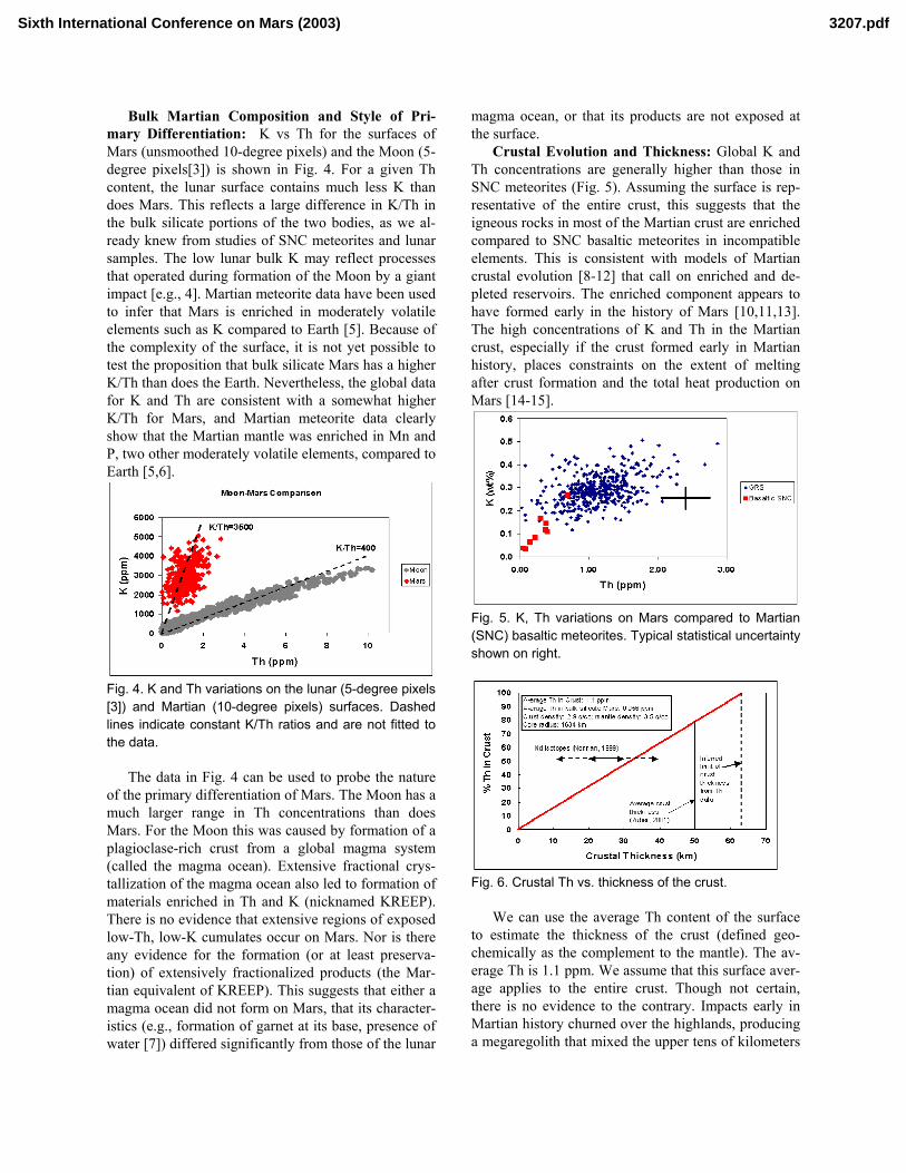
Bulk Martian Composition and Style of Pri-mary Differentiation: K vs Th for the surfaces ofMars (unsmoothed 10-degree pixels) and the Moon (5-degree pixels[3]) is shown in Fig. 4. For a given Thcontent, the lunar surface contains much less K thandoes Mars. This reflects a large difference in K/Th inthe bulk silicate portions of the two bodies, as we al-ready knew from studies of SNC meteorites and lunarsamples. The low lunar bulk K may reflect processesthat operated during formation of the Moon by a giantimpact [e.g., 4]. Martian meteorite data have been usedto infer that Mars is enriched in moderately volatileelements such as K compared to Earth [5]. Because ofthe complexity of the surface, it is not yet possible totest the proposition that bulk silicate Mars has a higherK/Th than does the Earth. Nevertheless, the global datafor K and Th are consistent with a somewhat higherK/Th for Mars, and Martian meteorite data clearlyshow that the Martian mantle was enriched in Mn andP, two other moderately volatile elements, compared toEarth [5,6].

Fig. 4. K and Th variations on the lunar (5-degree pixels[3]) and Martian (10-degree pixels) surfaces. Dashedlines indicate constant K/Th ratios and are not fitted tothe data.

The data in Fig. 4 can be used to probe the natureof the primary differentiation of Mars. The Moon has amuch larger range in Th concentrations than doesMars. For the Moon this was caused by formation of aplagioclase-rich crust from a global magma system(called the magma ocean). Extensive fractional crys-tallization of the magma ocean also led to formation ofmaterials enriched in Th and K (nicknamed KREEP).There is no evidence that extensive regions of exposedlow-Th, low-K cumulates occur on Mars. Nor is thereany evidence for the formation (or at least preserva-tion) of extensively fractionalized products (the Mar-tian equivalent of KREEP). This suggests that either amagma ocean did not form on Mars, that its character-istics (e.g., formation of garnet at its base, presence ofwater [7]) differed significantly from those of the lunar

magma ocean, or that its products are not exposed atthe surface.

Crustal Evolution and Thickness: Global K andTh concentrations are generally higher than those inSNC meteorites (Fig. 5). Assuming the surface is rep-resentative of the entire crust, this suggests that theigneous rocks in most of the Martian crust are enrichedcompared to SNC basaltic meteorites in incompatibleelements. This is consistent with models of Martiancrustal evolution [8-12] that call on enriched and de-pleted reservoirs. The enriched component appears tohave formed early in the history of Mars [10,11,13].The high concentrations of K and Th in the Martiancrust, especially if the crust formed early in Martianhistory, places constraints on the extent of meltingafter crust formation and the total heat production onMars [14-15].

Fig. 5. K, Th variations on Mars compared to Martian(SNC) basaltic meteorites. Typical statistical uncertaintyshown on right.

Fig. 6. Crustal Th vs. thickness of the crust.

We can use the average Th content of the surfaceto estimate the thickness of the crust (defined geo-chemically as the complement to the mantle). The av-erage Th is 1.1 ppm. We assume that this surface aver-age applies to the entire crust. Though not certain,there is no evidence to the contrary. Impacts early inMartian history churned over the highlands, producinga megaregolith that mixed the upper tens of kilometers


of the crust, as we suspect happened on the Moon.Dust and soils might represent at least a rough averageof the upper crust. Finally, lava flows exposed on thesurface might be similar in composition to magmasintruded at depth.

Assuming that this applies to the entire crust andthat the primitive mantle had a Th concentration of0.056 ppm [5], we find that 100% of the Th would bein a crust 65 km thick (Fig. 6). Since 100% partition-ing of Th is unlikely, this is the maximum crustalthickness. If the average crustal thickness is 50 km[16], then the crust contains about 65% of the planet'sbulk Th, in agreement with Norman's [8] estimate that50-55% of the Nd is in the crust. This level of differ-entiation is not greatly different from that of the Earth.

K and Th as Monitors of Aqueous Alteration:The K/Th ratio varies considerably on Mars (Fig. 3, 5).These elements behave reasonably conherently duringigneous processing. Although they do vary somewhatamong major groups of igneous rocks on Earth, theirgeochemical behavior during partial melting and frac-tional crystallization are very similar compared to theirbehavior during aqueous processing. We cannot ruleout fractionation by igneous processes, especially atthe extremes of fractionation [S. McLennan, personalcommunication]. K/Th varies among basaltic SNCmeteorites (Fig.5), though not to the extent it varies inour global data set. The Moon provides an excellentexample of fractionation under extensive igneousprocessing, and the global data obtained by LunarProspector indiates that K/Th is relatively constant(Fig. 4). Thus, we are pursuing the idea that the varia-tion in K/Th is caused at least in part by aqueous proc-esses. We hope this ratio, and U data when countingstatistics improve, will be a useful tool for studyingaqueous processes on a global scale.

Fig. 7. Weathering of terrestrial basalt causes a deple-tion of K while Th remains constant, leading to reduc-tion in the K/Th ratio.

Dissolution of K and Th depends on the solubilityof the phases they are in: K in feldspar (plagioclase

and K-feldspar) and volcanic glass, and Th in phos-phates, volcanic glass, and possibly in other accessoryphases such as zircon and monazite. Experiments andmeasurements of weathering profiles illustrate the dif-ferent behavior of K and Th. Nesbitt and Wilson [17]studied a terrestrial weathering profile in basalt (Fig.7). Th is resistant to transport while K is very mobile.In this example, both K and Th were concentrated inresidual glass in the lava flow studied.

Dreibus et al. [18; also Dreibus and Wanke, un-published data] did leaching experiments on the Mar-tian meteorites. They put pulverized meteorite powdersin slightly acidic, saturated solutions of Mg2SO4, andallowed the powders to be leached for minutes tohours. The results (Fig. 8) show that the REE and Uwere almost completely removed from the residue,while almost all of the K remained undissolved. Theyinterpreted this to indicate that the leached elementswere all contained in phosphates, while K was con-fined to plagioclase. This is another illustration thataqueous processes can fractionate K from U, and pre-sumably from Th. (Th could not be measured by theINAA technique used, but would probably have be-haved like U because it is contained in phosphates,too. Its behavior in the solutions might be very differ-ent from that of U, however.) Because P is abundant inSNC meteorites (and by inference in the Martian man-tle), phosphate dissolution might be important in frac-tioning K from Th.

Fig. 8. Leaching experiments [18] on Martian meteor-ites show that mildly acidic solutions rapidly dissolvephosphate minerals, removing REE, U, and (presuma-bly) Th from the residual solid. Terrestrial basalts maybehave differently because of differences in siting ofthese trace elements.

Differential solubility of K-bearing phases and Th-bearing phases may have led to large-scale fractiona-tion of K and Th, as shown in Fig. 3. The K/Th ratioand total abundances of each might serve as a monitorof global fractionation caused by aqueous processes


(weathering, hydrothermal alteration, fumerolic activ-ity, etc.). However, to use this tool, we need more ex-periments and detailed geochemical modeling of traceelement fractionation under Martian environmentalconditions.

Conclusions: Although our data should still beconsidered preliminary, we can make some tentativeconclusions: (1) The concentrations of K and Th andthe K/Th ratio vary across the Martian surface. (2) Theconcentrations are significantly higher than those inSNC meteorites, suggesting different mantle sourcesfor the meteorites compared to the bulk of the crust.(3) Most of the crustal igneous rocks could haveformed from enriched mantle sources. (4) The con-centration of Th on Mars does not vary as much as itdoes on the Moon, suggesting that the primiary differ-entiation of Mars differed from that of the Moon. (5) Ifthe average Th concentration of the surface is equal tothe average of the entire crust, the crust cannot bethicker than 65 km. (6) The mean Th concentration isconsistent with a crust 10s of km thick. (7) Aqueousprocesses have played an important role in the frac-tionation of K from Th.

Acknowledgments: We thank all members of theGRS team for instrument, data reduction, and com-puter support. This work is supported by NASA.

References: [1] Boynton, W. B., et al. (2003) LPSXXXIVI, Abstract #2108. [2] Reedy, R. et al. (2003) LPSXXXIV, 1592. [3] Prettyman, T. H, et al. (2002) LPS XXXIII,Abstract #2012. [4] Drake, M. J. and Righter, K. (2002) Na-ture 416, 39-44. [5] Wänke, H. and Dreibus, G. (1988) Phil.Trans. R. Soc. Lond. A 325, 545-557. [6] Halliday, A. et al.(2001) Space Sci. Rev. 96, 197-230. [7] Hess, P.C. and Par-menier, E. M. (2001) LPS XXXII, Abstract #1319. [8] Nor-man, M. D. (1999) MAPS 34, 439-449. [9] Norman, M. D.(2002) LPS XXXIII, Abstract #1175. [10] Borg, L. et al.(1997) Geochem. Cosmochem. Acta 61, 4915-4931. [11]Wänke, H. et al. (2001) Space Sci. Rev. 96, 317-330. [12]McLennon, S. (2002) LPS XXXIII, Abstract #1280; alsosubmitted manuscript. [13] Halliday, A. et al. (2001) SpaceSci. Rev. 96, 197-230. [14] McLennan, S. (2001) Geophys.Res. Lett.28, 4019-4022. [15] Hauck, S. and Phillips, R. J.(2002) J. Geophys. Res. 107, 10.1029/2001JE001801. [16]Zuber, M. T. (2001) Nature 412, 220-227. [17] Nesbitt, H.W. and Wilson, R. E. (1992) Am. J. Sci.292, 740-777.[18] Dreibus, G. et al. (1996) LPS XXVII, 323-324.


THE MICROSCOPE FOR THE BEAGLE 2 LANDER ON ESA’S MARS EXPRESS. N. Thomas1,2, S.F. Hviid1,H.U. Keller1, W.J. Markiewicz1, T. Blümchen1, A.T. Basilevsky1,3, P.H. Smith4, R. Tanner4, C. Oquest4, R. Reynolds4,J.-L. Josset5, S. Beauvivre5, B.Hofmann6, P. Rüffer7,C.T. Pillinger8, M.R. Sims9, D. Pullan9, and S. Whitehead9

1Max-Planck-Institut für Aeronomie, Max-Planck-Str. 2, D-37191 Katlenburg-Lindau, Germany, 2PhysikalischesInstitut, University of Bern, Sidlerstr. 5, CH-3012 Bern, Switzerland, 3Vernadsky Institut, Moscow, Russia, 4Lunar andPlanetary Lab. University of Arizona Tucson, Arizona, U.S.A., 5Micro-Cameras & Space Exploration (SPACE-X),Neuchatel, Switzerland, 6Natural History Museum, Bern, Switzerland, 7Institut für Datentechnik undKommunikationsnetze der TU Braunschweig, Braunschweig, Germany, 8Dept. of Earth and Planetary Sciences, OpenUniversity, Milton Keynes, U.K., 9Dept. of Physics and Astronomy, University of Leicester, Leicester, UK.

Introduction: The European Space Agency (ESA)will launch the Mars Express spacecraft in June 2003.The mission is intended to provide a flight opportunityfor re-builds of experiments lost as a result of theRussian Mars "96 launch failure and will reach Marsaround Christmas 2003. The re-build has allowed severalinstruments to be improved and upgraded. However, acompletely novel element of the Mars Express payloadis the Beagle 2 lander.

Beagle 2 is designed to descend through the atmo-sphere of Mars to the surface using a combination ofaerobraking, parachutes, and airbags. After coming torest in the Isidis Planitia region of Mars, (260-270�W,5-10�N), the lander will deploy solar panels and beginscientific operations. The scientific payload comprises anX-ray fluorescence spectrometer, a Mössbauer spectrom-eter, a stereo camera system, a stepped combustion massspectrometer (GAP), a sampling device (``PLUTO''), aset of environmental sensors, and a microscope.

Most of the experiments (the exceptions being theGAP and the environmental sensors) are mounted on arobotic arm referred to here as the ARM. The end of theARM has a flat experiment "platform", referred to as thePAW (position adjustable workbench), on which theexperiments are mounted.

In addition to the experiments, a grinding and coringtool is also available on the PAW to scratch and flattenthe surfaces of rocks within reach of the ARM.

This paper describes the aims and performance of themicroscope on the Beagle 2 PAW.

Scientific Objectives: A microscope has fourdistinctly different tasks in a lander package. Firstly, theinstrument can be used to study the physical and struc-tural properties of a surface and hence make a geophysi-cal analysis and contribute to the overall geological andmineralogical interpretation of the landing site.

Secondly, a microscope can contribute to studies ofthe atmosphere of Mars. Specifically, dust particles are

continuously precipitating out of the dusty atmosphereand hence a microscope can be used to constrain thesizes and shapes of particles for input into atmosphericscattering and radiative transfer models of the Martianatmosphere.

Thirdly, the instrument can be used to characterizeand/or select a sample before it is passed to anotheranalytical instrument. It is used therefore to assist thechemical analysis.

Finally, the instrument can be used to study themorphology of a potentially biological sample and henceidentify structures which are characteristic of past orpresent biological activity.

Instrument Concept: The concept of the optics forthe microscope was based on a system originally de-signed for the Mars Environmental CompatibilityAssessment (MECA) experiment package which wasslated for launch on the cancelled Mars "01 mission.

The detailed design of the microscope for Beagle 2was constrained by even more stringent mass andvolume limits. This suggested that we try to keep thefocal length of the experiment as short as possible. This,in turn, implied that we should select a relative shortworking distance (the distance between the objectposition and the first optical element) of the order of 12mm. This was considered a reasonable solution giventhat the ARM would be able to bring the microscope tothe sample. The optically active elements comprise aCook triplet. The optics provides a magnification of3.5:1.

The sample is unlikely to be well illuminated bysunlight because the microscope itself shadows thesample. This implied that an illumination system wouldbe required. Microscopes in the laboratory use eithertransmissive illumination or confocal illumination.While a confocal system is desirable, at present thedevelopment of such a method of illumination forspaceflight is only at a preliminary stage. For Beagle 2,


Figure 1 The FM microscope views a target mountedon a translation stage during bench testing.

Figure 2 Microscope image of yeast on agar. Thefield of view is 4 x 4 mm2. The brights dots on thesurface of the yeast come from specular reflectionsfrom the LEDs. Individual organisms are below theresolution limit.

we have chosen to use light-emitting diodes (LEDs)mounted around the entrance aperture of the microscope.The system comprises 12 LEDs, 3 red, 3 green, 3 blueand 3 UV. The UV LEDs are designed to induce fluores-cence in rocks (or a biological sample). A filter has beenintroduced into the optics to eliminate reflected UV fromthe incoming beam.

For mass reasons, it was decided to use a mi-cro-camera head including a CCD detector and itsassociated electronics (detector control electronics,analogue to digital converter, noise reduction filters,clock, memory buffer, serial digital interface drivers, and10 Mbit s-1 communication protocol) in a lightweight(ca. 80 g) highly integrated 3D module. This mi-cro-camera has benefited from developments bySPACE-X within a contract from the ESA TechnicalResearch Programme (TRP). The 14 micron pixel pitchleads to a pixel scale of 4 micron px-1. The CCD is a 1k

x 1k device giving a field of view of just over 4 x 4 mm2.Even before detailed design commenced it was clear

that the depth of focus of the microscope would be under100 microns. It was also apparent that the accuracy withwhich the PAW could bring the microscope to thesample would be at least a factor of 20 larger than this.Thus, a focussing mechanism was necessary. Translationof the entire microscope at the interface to the PAW wasimplemented. The PAW provides a means of bringingthe microscope to within ±3 mm of its target. A "thumb"on the PAW prevents the microscope from impacting

rocks unless their surface roughness is greater than ±12mm (the working distance). The full range of the steppermotor is ±3 mm, matching the accuracy of the PAWmotion. The instrument is shown in Fig. 1.

Test Results: An image scale of 4.075 micron px-1 atthe best focus position was derived in bench tests. Thevariation in the image scale across the field of view ofthe microscope corresponds to a 0.2% distortion. TheFWHM of a point source at the nominal focus positionis 4.50 microns (1.10 px) and is less than 6 microns (1.5px) within 50 microns of the nominal focus position.This result indicates that the accuracy of the steppermotor motion (20 microns) should be more than suffi-cient.

The flat-field shows some slight evidence of vignett-ing at the corners of the FOV. This is partly due to aslight misalignment of the detector in its housing andpartly due to the baffling system.

The red LEDs are slightly susceptible to temperatureand their central wavelength decreases from nominal(642 nm) at room temperature to 625 nm at 183 K. Thewavelengths of the other LEDs vary by less than 2 nmover this temperature range. The output of the UV LEDsis strongly temperature dependent below 220 K and theybecome very faint below 200 K.


The illumination field has been calibrated for all LEDcombinations and the system absolute response com-puted. (Care needs to be taken here because, unlike mostimagers, the microscope also provides the irradiance ofthe target.)

For amusement we show in Figure 2 an image ofsome yeast grown on agar. This shows that the micro-scope still does not have high enough resolution toresolve individual organisms.

Flight Software: The microscope can generate ahuge volume of data. In particular, because we have noa priori knowledge of the focus position and becausedifferent parts of the field will have different focuspositions as a result of surface roughness, many imagesat different positions need to be acquired to ensure thatall parts of the field are in focus at some point. Poten-tially, 60 or more images may be required to guaranteethat we obtain all parts of the field in focus at somestage.

Two approaches to solving the problem of datavolume have been implemented on Beagle 2. Firstly, awavelet compression algorithm has been incorporatedinto the lander software to reduce the total data volumefrom the experiment. The algorithm will also be used tosupport the other imaging experiment (the stereo pan-oramic camera) onboard Beagle 2. Wavelet compressorsresolve the image into a series of coefficients which arerelated to spatial frequencies. The more detail one wishesto see in an image, the more coefficients one has toreturn. For the microscope this scheme is extremelyeffective. The reason is because an out of focus imagedoes not require many coefficients. It is smooth. There-fore, unfocussed frames compress extremely well withratios in excess of 40:1 often achievable with almost noloss. Hence, one possibility is to transmit all 60 framescompressed according to a quality criterion.

The second approach is to analyse the data onboard.Here we acquire all 60 frames but investigate the entropyat each position in each image to determine which imagehas the best focus for that position. We then downlink acompletely focussed composite image.

In both cases, an important result from the analysisis that the image in which focus has been achieved for aposition allows us to define unambigiously its depth.Hence, not merely does the microscope gives us a 2-Dpicture of the surface, it also gives us a depth mapallowing complete 3-D reconstruction of the surface.

Summary: The microscope for Beagle 2 is a highlycompacted (160 g) device which will provide 6 micronresolution images of surface material in Isidis Planitia.The elegant design of the system makes it ideal forfuture landed missions where microscopic imagingmight be required. Adaption of the system to supportother experiments (e.g. Raman spectrometer or lasermass spectrometer) should be relatively straightforward.

This abstract is a summary of a more detailed instru-ment paper submitted to Planetary and Space Science.

Acknowledgments: The development of the micro-scope optics was funded by the University of Arizona'sspecial fund. The micro-camera head was sponsored bySPACE-X. The Max-Planck-Gesellschaft supportedintegration and test. Software development was partlysponsored by DLR. The Beagle 2 PAW microscopefocussing mechanism was funded by the Particle Physicsand Astronomy Research Council of the UK. M.R. Simsacknowledges funding from the University of Leicesterand via the Royal Society Industry Fellow scheme.


THE SOUTH POLAR RESIDUAL CAP OF MARS: LANDFORMS AND STRATIGRAPHY. P. C. Thomas1 1Center for Radiophysics and Space Research, Cornell University, Ithaca NY, 14853.

The south polar residual cap (sprc) of Mars is morphologi-cally distinct from that in the north, and is largely composi-tionally distinct as well, apparently dominated by CO2 rather than the H20 present in the northern residual cap. This work addresses questions of the history and signifi-cance of these distinctive deposits by mapping the many forms using MOC images and MOLA data. Depositional units: There are two primary sets of deposi-tional units in the sprc: 1) An older unit, approximately 11 m in thickness with four included layers, widely distributed over the sprc, and expressed as mesas or broad surfaces cut by a variety of circular to linear depressions, and com-monly having polygonal troughs (Fig. 1a). 2) One or more younger units, approximately 2 m thick, that have superposed and filled depressions formed in the older unit, and also formed in local discrete deposits. This unit also has a wide variety of depression types (Fig. 1b, c) Both of these sets of units occur on the flatter topography of the polar deposits (slopes under 2°), and terminate in troughs at elevations only a few m lower than where the layers are fully developed. Both units show scarp retreat of up to a few m over one Martian year [1]. Erosion and other modification forms: The sprc topog-raphy has unique erosional topography [2,3]. There are a great variety of these forms, many are seen to merge into other forms. While the large circular depressions have received the most attention, these are not even the “typical” form. We have mapped the following forms: generic de-pressions, large circular depressions, parallel sets of linear depressions (fingerprint terrain), other linear depressions, moats, and curled depressions, among others Fingerprint depressions define a few coherent patterns, and are not simply oriented with one side toward the pole; their consistent trends suggest underlying structural control; their shapes show common upper surface fracture control (Fig. 1e). They occur in a restricted area of the sprc (Fig. 2a). The curl depressions (Fig. 1d,f) are oriented with openings dominantly within 60° of north (Fig. 2d). The surface in-denting the curl commonly is in a ramp form (Fig. 1f), rather than a pedestal. Moat-like depressions occur within some nearly circular forms as well as bounding a variety of mesas and other remnant topography. Moats within other depressions show two distinct widths: ~20 m and ~70 m. The latter is indis-tinguishable from moat widths around mesas and other remnants (Fig. 2c). Development of the depressions and deposits: Changes between 1999 and 2001 indicate some backwasting of the forms of order 1-4 m/ Mars year [1], with a few instances over 5 m. Initiation of the forms, and enlargment of many, however, involve mechanisms other than backwasting of steep scarps. Disruption of the older upper surface occurs at least in part by sag and collapse; development sequences of curled depressions can be found, and examples of en-largement almost entirely by collapse are also found (Fig. 1d,i). The sag and collapse features may explain the de-

velopment of “escher” terrain, whereby an upper surface appears contiguous between different cycles of erosion (Fig. 1j). Thin layers preferentially develop pits and other depres-sions over underlying topography, and on some upper con-vex slopes (Fig. 1b). These pits, “peels”, and moats indi-cate modification of overlying deposits by exposure of relief or a critical layer thickness. There are examples of inverted relief, wherein the older, thick deposits have col-lapsed after deposition of thin deposits within the large depressions . Non-uniform deposition is also found in some tongues of material several m in depth and a few hundred m long in restricted areas of the sprc. These appear to be part of the later deposits. Pattered ground: Slopes from remnants of the thick, older unit commonly show surfaces with brick or cobblestone appearance, sometimes giving a false impression of large numbers of layers exposed in the mesas (1a). Material underlying the sprc in some troughs displays a slightly different patterned appearance. Interpretations: Several different cycles/changes in polar depositional and sublimational regime are indicated: 1). Change from main polar layered deposits to deposition of the 11 m set of layers: H20 rich deposits to CO2 rich ones. 2) Cycles producing layering within the 11 m stack, about 4 cycles. Some differences in physical charac-teristics/ composition. 3) Significant erosion of the deposits in the form of merging depressions and sag and collapse modification. 4) Before or during the subsequent steps, devel-opment of polygonal troughs in much of the surface of the thick deposit. 5) Deposition of one or two, ~ 2 m layers in the erosional topography of the thick deposits. 6) Renewed sublimation of both deposits. In-cluded in this step is the scattered development of inverted relief. This activity may continue at present. The primary interpretive difficulty is the similarity and merging of deposits formed by sag and collapse of the thick units, and thinner, younger layers (step 5 above). Both units are clearly present; however, which is present at a particular site is sometimes unclear. The evident variety of layer types, thicknesses, and cycles of deposition and erosion (including inverted relief) show there are several combinations of composition and/or tex-ture within these deposits. More than one type of climate cycle is required to form these features’ current appear-ance. References: [1] Malin, M. C., M. A. Caplinger, and S. D. Davis (2001). Science, 294, 2146-2148. [2] Thomas, P. C. et al. (2000). Nature 404, 161-164. [3] Byrne, S., and A. P. Ingersoll (2003). Science 299, 1051-1053.


Acknowledgements: Help was provided by Mike Malin, Ken Edgett, Scott Davis, Bruce Cantor, Rob Sullivan, and Lisa Wei.

Figure 1a. Surface of thicker sprc unit, with polygonal troughs and darker patterned materials flanking slopes of 3-4 layers. Moat to the right. b). Erosion of thinner layers in places follows underlying topography, here part of a curving ridge in the lower left. Sun from lower right. c. Thinner unit eroded in moat from underlying topography. d. Depressions with fracture boundaries showing development sequence toward a curl depression. e. Fingerprint trough. f. Curl trough, showing interior ramp. g. Con-fined moats. h. Moat, showing textured lower surface, probably the main polar layered deposits. i. Linear depression and sag. j. “Escher” terrain with uncertain relation of upper and lower surfaces, probably generated in part by sag and collapse as in Fig. 1 i.


Figure 2. Some characteristics of the south polar residual cap erosional forms. a) Location of fingerprint terrain. b) Locations of upper surface of thick unit (circles), and most kinds of moats (small dots). Both forms are widespread over the sprc. Locations of changes measured in excess of 3 m in one Mars year shown by x’s (Measured change is 6 m or more across walls or depres-sions; single distance is 3 m or more.) c) Widths of some depression types. Note the similarity of open and confined moats and linear depressions; slight distinction of the fingerprint depressions. d) Orientation, clockwise from north, of the curl depressions. The orientation would be to the left in Fig. 1f.


CARBONATES ON MARS: PROBABLE OCCURRENCES, SPECTRAL SIGNATURES, ANDEXPLORATION STRATEGIES. B. J. Thomson and P. H. Schultz, 1Brown University, Department of Geologi-cal Sciences, Box 1846, Providence, RI 02912 ([email protected]).

Synopsis: Carbonates and other aqueous alterationproducts occur in the SNC meteorites [1,2], and spec-tral observations suggest that carbonate is present inMartian dust as a minor constituent [e.g., 3-7]. Analy-sis of analogous terrestrial dust deposits (loess) in Ar-gentina, which also contain a significant carbonatecomponent, has revealed that post-depositional modifi-cation of the loess can result in the reprecipitation ofcarbonate as concretions and as discrete layers of cal-crete. These Argentine deposits give us a roadmap forlocating the most accessible carbonate deposits onMars.

Introduction and background: The presence ofcarbonates on Mars has long been surmised as a sinkfor CO2 on the basis theoretical models of the evolu-tion of the Martian atmosphere [8,9]. The character,abundance, and distribution of carbonates are impor-tant parameters for assessing the paleoclimate andvolatile evolution of Mars.

Carbonates have been tentatively identified withspatially coarse telescopic spectral studies [e.g., 2-6].With higher spatial resolution data of TES, regionaloutcrops (>10km2) of moderately-grained carbonate-rich material were not detected, despite a thoroughsearch [8]. However, recent analyses of the carbonateabsorption feature near ~7µm in TES data has identi-fied fine-grained carbonates at the ~2-3wt% level inMartian dust [7].

The dust appears to have been globally homoge-nized and is decoupled from the underlying surface.The distributed carbonate component in the dust islikely derived from the weathering of more concen-trated sources. A lack of regional carbonate-rich out-crops may indicate that primary carbonate deposits areeither mantled or deeply buried.

Additional information about the ultimate fate ofcarbonates is provided by the SNC meteorites, ofwhich all subgroups contain traces of water-depositedminerals [1]. The formation ages of these secondarymineral assemblages tell us about the timing of fluidflux through the upper crust of Mars. Radiometricages of the carbonates range from ~4 Ga to ~0.7 Ga inALH84001 and Nakhla, respectively [9,10]. Coupledwith the lack of extensive alteration of the silicatephases, this indicates that the responsible fluids did notspend a long time in contact with these rocks but wereintermittently active over the bulk of Martian history.The upper crust of Mars may have experienced epi-

sodic “wetting events” that leached and reprecipitatedcarbonates in the subsurface.

Carbonates in loess. We propose that the post-depositional evolution of carbonates in Martian dustmay be similar to the evolution of carbonates in Ar-gentine loess deposits. Carbonates are present in twoforms in the loess: they are found as fine-grained dis-tributed components and are also concentrated intoconcretions or calcrete layers (Figure 1). The carbon-ate fraction of typical Argentine loess varies betweenabout 2-4% [11].

Accumulations of carbonate, locally known astoscas, are widely distributed throughout Argentineloess sequences [12]. Formed through the downwardleaching and reprecipitation of soluble componentsinto lower soil horizons, these illuvial calcretes de-velop in situ and may cement and/or replace the hostmaterial. The calcrete morphology can be highly vari-able depending on the degree of development and localstructural control. Observed forms include concretionsor nodules, reticular and string-like patterns, and layersor hardpans (see Figures 1,2) [12]. These carbonatescan generally be classified as pedogenic calcretes [13],although some sections may contain additional carbon-ates derived from laterally moving groundwater (whichis not strictly a pedogenic process). The salient pointis that carbonates are a mobile component in the sub-surface that commonly form local concentrations ofcalcrete.

Spectral detection of carbonates: The planercarboxyl (CO3

2-) ion has six fundamental vibrationalmodes, of which two are degenerate and one is infraredinactive [e.g., 14,15]. The exact shape and position ofvibrational absorption bands varies with the cationspecies: e.g., calcite (Ca), dolomite (Ca,Mg), magne-site (Mg), and siderite (Fe). The strongest infraredabsorption features in calcite occur at 7.0 µm (asym-metric stretch), 11.4 µm (out-of-plane bend), and 14.0µm (in-plane band) [15]. Additional combination andovertone features are present in the near infrared.

Detecting carbonate absorption features in field ex-posures of carbonates can be difficult due to the loss ofspectral contrast from surface roughness at a variety ofscales [16]. This includes roughness at the outcropscale between individual boulders and cobbles, roughsurface textures on exposed blocks, and microscopicroughness [17]. We are in the process of documentingthe spectral signature of calcrete layers exposed in


FINDING MARTIAN CARBONATES: B. J. Thomson and P. H. Schultz

section in loess deposits in the visible, near-infrared,and thermal infrared regions to assess the detectabilityof these deposits with rover-mounted instrumentation.

Exploration strategies: The most readily accessi-ble concentrations of carbonates on Mars are likelyreprecipitated calcrete layers within dust deposits. Thepotential for entombment and preservation of organicmaterial in chemical precipitates makes these layers ahigh-priority target for exobiology [18]. Depending onthe degree of cementation, these calcretes may formresistant hardpans that are exposed through differentialerosion. However, due to mantling by continued dustdeposition, exposed calcrete horizons may be difficultto spectrally detect. In addition, terrestrial calcretehardpans are known to weather to boulders, cobbles,and smaller fragments [19] that will increase macro-scopic roughness and reduce spectral contrast, thusfurther complicating spectral detection.

Perhaps a more likely locale where an unambigu-ous spectral signal may be obtained is in high slopeareas where the subsurface profile is exposed (i.e.cliffs, mesa edges, channel walls). Calcrete layers tendto form steeply inclined surfaces in vertical exposuresdue to their high mechanical strength and thus may berelatively dust-free and clear of fragmental material.They may be more readily identifiable with visi-ble/near-infrared imaging Pancam and thermal infraredspectrometer Mini-TES on the 2003 Mars ExplorationRovers than from orbital imaging/spectral platforms.

Another potential target of interest for sample-return missions is impact glasses derived from carbon-ate-bearing lithologies. Chemical systematics in im-pact glasses of various ages could provide a record ofthe isotopic evolution of the Martian atmosphere [20].

References: [1] Gooding J. L. (1992) Icarus, 99,28-41. [2] Bridges J. C. et al. (2001) Space Sci. Rev.,96, 365-392. [3] Blaney D. L. and McCord T. B.(1989) JGR, 94, 10,159-10,166. [4] Pollack J. B. et al.(1990) JGR, 95, 14,595-14,627. [5] Calvin W. M. etal. (1994) JGR, 99, 14,659-14,675. [6] Lellouch E. etal. (2000) Planet. & Space Sci., 48, 1393-1405. [7]Bandfield J. L. et al. (2003) LPS XXXIV, abstract#1723. [8] Christensen P. R. et al. (2001) JGR, 106,23,823-23,871. [9] Borg L. E. et al. (1999) Science,286, 90-94. [10] Swindle T. D. (2000) Met. Planet.Sci., 35, 107-115. [11] Teruggi M. E. (1957) J. Sed.Petrol., 27, 322-332. [12] Zarate M. A. and Fasano J.L. (1989) Palaeogeo., Palaeoclim., Palaeoeco., 72, 27-52. [13] Goudie A. S. (1983) in Chemical Sedimentsand Geomorph., Academic Press, 93-131. [14] ClarkR. N. (1999) in Remote Sensing for the Earth Sciences,John Wiley & Sons Inc., 3-58. [15] van der Marel H.

W. (1976) Atlas of Infrared Spectroscopy of Clay Min-erals and their Admixtures, Elsevier Sci. Pub. Co., 396pp. [16] Kirkland L. et al. (2002) Remote Sens. Env.,80, 447-459. [17] Kirland L.E. et al. (2002) Proc.SPIE, 4495, 158-169. [18] Farmer J. D. and DesMarais D. J. (1999) JGR, 104, 26,977-26,995. [19]Netterberg F. and Caiger J. H. (1983) in Residual De-posits, Blackwell Sci. Pubs., 235-243. [20] Delano J.W. (1988) LPI Tech. Rpt. 88-07, 63-64.

Figure 1. Sea-cliff exposure of loess in Argentina showingsingle well-developed calcrete layer.

Figure 2. Exposure of loess sequence in Argentina showingmore complex morphology of calcrete deposits.


GREAT MARTIAN DUST STORM PRECURSOR?. J. E. Tillman, Department of Atmospheric Sciences, University of Wash-ington, Seattle, WA, USA ([email protected]).

Reviews of rejected proposals for analyses of Viking lan-der meteorology data sometimes have stated that nothing sig-nificant remains to be learned: it is proposed that lander tem-perature differences between the first and second year prior tothe dust storm season, may be related to or even be used as apredictor of whether or not great dust storms form later in theyear. The Viking lander mission demonstrated conclusivelythat some years have great dust storms while others do not,contrary to conventional wisdom prior to the Viking resultswhich suggested that they occurred every year. The first yearhad two, beginning at about L s 210 (1977 A) and 310 (1977B), the second and third had none, while the fourth year hadone that was initiated about L s 200 (1982).

Atmospheric temperature data were processed and aver-aged into 25 segments/sol, i.e., roughly hourly averages foralmost all of the Lander 2 but far less than half of the Lander1 mission. (The Lander 1 data were only partially processeddue to problems with the wind determination.) From these, theminimum, sol average and maximum temperatures were de-termined for each sol. Lander 2 temperatures between roughlyL s 117 and 177, prior to the beginning of the great dust stormseason, show that the minimum and daily average tempera-tures were essentially identical for the first year, with, and thesecond year, without, great dust storms, while the maximumtemperature for the first year was consistently lower on a solby sol basis by 3 to 9 degrees Celsius. This implies that thefirst year was dustier than the second and poses the question“Do these temperature differences truly indicate optical depthchanges, and thereby atmospheric heating changes, and if soare these responsible for the presence or absence of great duststorms later in a given year?” Alternatively, are they artifactsor not significantly material to the circulation later in the year.The Lander 2 evidence for this possible dust storm precursor

condition will be presented.

Unprocessed Lander 1 data exist that can support or refutethis hypothesis for most of this same season during years 1 and2, a small portion of year 3, and for the first part of year 4 priorto its great dust storm. Lander 1 data have been processedfor this season only in year 1, due to problems with the windsensors that do not directly affect the temperature observations.(These wind sensor partial failures occurred in the first year, thefirst at L s 117 and the second at L s 303.) These unprocessedLander 1 temperature data should be processed and analyzedto support, refute or modify this hypothesis and be comparedwith other data related to optical depth such as the secondharmonic of the daily pressure variation which is a very goodoptical depth proxy. If these additional data are consistentwith this hypothesis, then they must be modeled to see if suchtemperature observations are great dust storm precursors andthereby can be used to forecast great dust storms later in thesame year. This potential illustrates why it is essential toreinstate climate observations as soon as possible, beginningat the Viking sites, and to make them permanent.

The Viking data are the only climate data for the surfaceof Mars and will remain so for the foreseeable future. It is nowpossible to far better process and analyze the Lander 1 winddata due to the dramatic improvement of computer resourcessince these efforts were terminated. Processing is still possiblesince all of the software, documentation and data have beenmaintained, without support, during the past decade and illus-trations of the additions to this surface meteorology climaterecord will be presented. It is essential that an internationalprogram be immediately initiated to understand, replicate, fur-ther process, and improve the Viking Lander meteorology cli-mate record, the only one for Mars, before this opportunity ispermanently lost.


TEMPORAL AND SPATIAL DISTRIBUTION OF SEASONAL CO2 SNOW AND ICE. T. N. Titus1 and H. H. Kieffer1, 1 U.S. Geological Survey, 2255 North Gemini Dr., Flagstaff, AZ 86001.

Introduction: The seasonal polar caps are a major element of Mars' climate and global atmospheric circu-lation. Theoretical calculations [1,2] and surface pres-sure measurements [3] indicate that about ¼ of the CO2 in the atmosphere condenses each year to form the seasonal caps. Changes in the polar cap albedo or emissivity modify the polar cap energy budget and the amount of CO2 condensation, consequently affecting the global martian climate.

Variations in both albedo and emissivity have been observed by several spacecraft. In the 1970s, space-craft observations of the polar regions of Mars re-vealed polar brightness temperatures that were signifi-cantly below the expected kinetic temperatures (140 - 148 K) for CO2 in sublimation equilibrium with the martian atmosphere[4]. The observational footprints were typically a few hundred kilometers in diameter, with 20 µm brightness temperatures (T20) as low as 130 K and had characteristic durations of a few days [4]. For historical reasons, we will refer to these re-gions as cold spots even though more recent observa-tions [5, 6, 7] support their kinetic temperatures being the same as the rest of the polar cap. A general lack of correlation between cold spots and Mars Global Sur-veyor (MGS) Mars Orbiter Laser Altimeter (MOLA) measurements of clouds and Thermal Emission Spec-trometer (TES) spectra suggest that most of the cold spots are surface regions of low emissivity. Occasion-ally, there are correlations to extremely dense polar night clouds and the “coldest” of the cold spots, sug-gesting a few of these cold spots may be “dry ice bliz-zards” in progress [6].

The MGS TES observations, combined with spec-tral modeling [5,7] using new CO2 optical constants [8], illustrate that the “cold spots” are due to fine-grain CO2, which cause a decrease in the 25 µm emissivity. Spectral models predict that fine-grain CO2 (hereafter referred to as snow, regardless of the formation proc-ess) has high albedo and low emissivity in the 25-µm-transparency band. Coarse-grained CO2 (hereafter referred to as ice) has low albedo (perhaps even trans-parent if the dust content is low) and near unit emissiv-ity. Increasing the dust content in the CO2 results in a large decrease in albedo, but only a slight increase in emissivity. TES observations have shown these ef-fects [9] for the southern springtime season cap, sug-gesting that the bright outliers (e.g. the Mountains of Mitchel) are snow covered, while other areas (e.g. the cryptic region) are mainly composed of ice.

The purpose of this paper is to present results from

the MGS TES continuing mission, showing the distri-bution of CO2 snow and ice in space and time. The dense coverage of the Mars polar regions by MGS TES has provided the ability to monitor the seasonal variations of condensates. Because TES has three sub-systems, we can monitor the distribution of solid CO2 in two ways: (1) monitoring the spectral differentiation between snow and ice and (2) the estimation of local CO2 mass accumulation.

The TES solar bolometer, combined with syntheti-cally derived brightness temperatures, can differentiate between snow and ice [9]. The difference between the estimated surface kinetic temperature, T18, and the brightness temperature in the CO2 25 µm transparency band, T25, effectively measures the emissivity at 25 µm and is taken as an indicator of the grain size of CO2 frost [5,6,9]. We will use the same convention as Titus el al. [6] where ice is defined as ∆T = T18-T25 < 5 K. This measure can be influenced by the presence of atmospheric dust, however that effect has not yet been quantified.

The TES directly measures the total reflected and emitted radiation, which in turn allow for the meas-urement of the geographic variation of the net radia-tion balance and, through integration of the inferred sublimation rates, the annual solid CO2 budget. We use the sublimation budget instead of the condensation budget to minimize the impact of lateral transport of heat during the polar night [5, 10]

Data: The MGS spacecraft orbit has an inclination of 93°, ascending (going north) on the night-side and going south (descending) on the dayside with a 14-hour Mars local time (H) equator crossing. For sim-plicity, we will refer to TES observations acquired on the ascending leg as AM and those acquired on the descending leg as PM. In normal mapping nadir-oriented mode, TES sweeps a 9 km wide swath along the sub-spacecraft track, which is almost parallel to meridians except near the pole. In this observation mode, the times between repeat coverage is highly dependent on latitude, ranging from only a few hours along the “polar rings” at ± 87° latitude to several days at ± 60º latitude. This allows detailed analysis of spa-tial and temporal changes near the polar caps. How-ever, at more equatorial latitudes seasonal analysis of specific locations is restricted due to the lengthy repeat time, approaching hundreds of days near the equator.


The TES data used were binned spatially into a po-lar stereographic projection with a mean resolution of 60 km per cell. Temporal binning was done on a base of 12 orbits (approx 23.55 hours). Missing data in the latitude/season cells were filled by linear interpolation in time.

Figure 1: North polar grain-size index, ∆T, at Ls = 342º. All polar figures have the same scale where the outer limits are at 45º latitude. The white plus in the center of the image is pole. Areas off the po-lar cap are white.

Snow and Ice Distribution: North Polar Distribution. The winter (or conden-

sation phase) cap is generally characterized by the ob-served 25 µm brightness temperatures (T25) near the expected surface temperatures for solid CO2, suggest-ing that direct surface condensation as slab ice occurs. Kieffer and Titus [5] and Titus et al. [6] show that cold spot observations, strong indicators of snow, are re-stricted to the perennial cap and other localized topog-raphical features, e.g. craters. We conducted a space-time analysis; our latest analysis is consistent with these prior results. The perennial cap has a high fre-quency of cold spot occurrence from approximately at Ls = 200º to approximately at Ls = 350˚.

The springtime (or sublimation phase) cap is gen-erally characterized by low ∆T, suggesting slab ice. However, by Ls = 45º a bright ring has formed just inside the receding cap edge. [Fig. 2] This bright ring is not visible in the ∆T image, suggesting that the brightening is not due to CO2 grain size effects. One plausible source of this bright receding ring is that water released from the season cap edge is redeposited as frost inside the cap [11].

During this same period of time, the perennial cap also appears bright without a corresponding increase in ∆T.

Figure 2: North polar cap albedo and grain-size index at Ls=38º. There is a lack of correlation be-tween these two parameters, suggesting that the brightening of the cap is due to water frost, not fracturing of CO2.

South Polar distribution: Cold spot activity in the southern winter starts approximately Ls=16º. The Mountains of Mitchel is one of the most active re-gions. Cold spot activity continues until approxi-mately Ls= 150º. After the sun has risen above the horizon, the cap begins to brighten, with the areas closest to the edge brightening first. A similar effect is


seen in ∆T, suggesting that the albedo brightening is due to an effective grain-size of the surface CO2 grain-size. Paige [12] explained this phenomenon as the fracturing of the surface ice due to insolation. TES observations are consistent with this explanation.

In many cases, the brightest springtime regions were areas of greatest winter cold spot activity. Per-haps wintertime accumulation of snow increases the likelihood that fracturing occurs in the spring.

Figure 3: South polar cap grain-size index at Ls=86º. The Mountains of Mitchel is one of the areas with high ∆T, suggesting the presence of snow.

Figure 4: South polar albedo and grain-size index at Ls=217º. Bright albedo areas generally have high ∆T, while areas with low albedo tend to have low ∆T.


Figure 5: Albedo vs. CO2 grain-size index. The data were restricted to springtime data with surface temperature less than 160 K. The red dots are for the south polar cap and the blue dots are for the northern polar cap.

Figure 6: North polar seasonal cap depth estimates. The black pluses are seasonal cap depths estimated from TES mass-balance calculations, assuming a CO2 density of 1606 km/m3. The red line is an es-timate from MOLA.

CO2 Mass Budget: The underlying assumptions in the TES mass balance calculations are that the total energy input into Mars is characterized by the solar bolometer and that the total energy out of the Mars system is characterized by the thermal bolometer. The energy difference between the input and output is as-sumed to be due to the sublimation or condensation of CO2. This implies that there is no geothermal heating or lateral transport of heat through the atmosphere. While initial estimates suggest that geothermal heating is negligible, a comparison of condensation and subli-mation mass budgets suggest that a large amount of heat transport does occur during the polar night [5,10]. However, comparisons of the sublimation budget to other observations [13] suggest that this technique is a

good estimate of actual amount of CO2 in the spring-time seasonal caps. For a detailed description of how the mass balance calculation is done, see Kieffer et al. [5] Figure 6 shows the estimated depth of seasonal CO2 if one assumes a pure substance (ρ = 1606 km/m3) compared to the seasonal depth estimated by MOLA [13]. If one assumes that the MOLA estimates are correct, we estimate the density of ice (latitudes south of 80ºN) as 1107±150 kg/m3 and the density of snow/ice mixture (latitudes north of 80ºN) as 979±133 kg/m3. The south polar MOLA depth estimates are not presented here because of possible systematic errors in the their depth estimates. When comparing MOLA and TES estimates, this offset must be ~20 cm to bring southern density estimates into agreement with the density for northern ice. A 20 cm offset is consistent with possible systematic errors for the southern data [14]. While these density estimates are preliminary, they are consistent with TES spectral observations of snow and ice distributions.

Conclusions: • The predominate form of CO2 condensation

is direct surface condensation as slab ice. • Regions with a high frequency of snow depo-

sition during the winter generally have brighter than average albedo in the spring, e.g. the Mountains of Mitchel.

• Springtime brightening of the south polar cap is predominately a change in grain size of the CO2. This is not the case for receding north-ern cap. Albedo variations are most likely dominated by the presence of water frost.

• An estimate of martian northern CO2 ice and snow/ice mixture densities based on combin-ing TES mass balance calculations and MOLA seasonal elevation changes are 1107±150 kg/m3 and 979±133 kg/m3, re-spectively.

References: [1] Leighton R. and Murry B. (1966) Sci., 153,

136-144. [2] Forget F. and Pollack J. (1996) JGR, 101, 16865-16879. [3] Tillman J. et al. (1993) JGR, 98, 10963-10971. [4] Kieffer H. et al. (1976) Sci., 193, 780-786. [5] Kieffer H. and Titus T. (2001) Icarus, 154, 162-180. [6] Titus T. et al. (2001) JGR, 106, 23181-23196. [7] Hansen G. (1999) JGR, 104, 16471-16486. [8] Hansen G. (1997), JGR, 102, 21569. [9] Kieffer H. et al. (2000) JGR, 105, 9653-9699. [10] Titus T. (2003) Mars Atm. Workshop, Granada, Spain. [11] Kieffer H. (2002) AGU Fall Mtg., Abstract P72C-02. [12] Paige D. (1985) , PhD Thesis.[13] Smith D. et al. (2001) Sci., 294, 2141- 2146. [14] Smith D. Per-sonal communication.


Correlation of Neutron-Sensed Water Ice Margins with Topography Statistics. R.L.Tokar1, M.A. Kreslavsky2,3, J.W.Head, III3, W.C. Feldman1, K.R. Moore1 and T.H. Prettyman1, 1Space and Atmospheric Sciences, MS D466, Los Alamos National Laboratory, Los Alamos, NM, 87545, [email protected], 2Kharkov Astronomical Observatory, Kharkov, Ukraine, 3Department of Geological Sciences, Brown University, Box 1846, Providence, RI, 02912.

Introduction: In [1], surface roughness and curva-

ture obtained from high resolution MOLA data are used to characterize a sedimentary mantle at high Mar-tian latitudes , (poleward of ~40º-60º). The equatorward boundary of the mantle correlates with the locations of dissected terrain identified in MOC images [2]. The dissected terrain in [2] is thought to be degraded water cemented soil, and the mantle discussed in [1] is in-ferred to be water ice rich. This conclusion is given further support in [3], where a positive correlation of the results in [1] and [2] is made with Odyssey neutron sensing of high hydrogen content in the near surface soil at high southern latitudes. The Odyssey data are measured by the neutron spectrometer (NS) component of the gamma ray spectrometer (GRS).

In this study, the margins between the water ice rich mantle and the relatively dry equatorial region are stud-ied for the northern and southern hemispheres using the Odyssey NS data and the MOLA rough-ness/curvature data. The position and extent in latitude of the margin is estimated via simulations of the NS data and the results are compared with average MOLA topography statistics . Preliminary results for two bands of longitude (120º-150º W and E) in the southern hemi-sphere are reported here.

Results: The following figure shows a map of the epithermal (0.4 eV < E < 700 keV) NS counting rate measured over the south circumpolar region during southern summer, as in [3]. Recall that low epithermal neutron count rate (blue region) corresponds to high hydrogen content of the near surface soil. See [4] for a complete overview of NS hydrogen estimates both at the poles and in the equatorial region. The black curve is the nadir position of Odyssey when the epithermal counting rate falls to ½ the maximum measured before encountering the water ice rich region. The margin re-gion studied here is the transition region near the black curve that delineates the water rich circumpolar mantle from the relatively dry equatorial region.

The following figure is a map of MOLA -derived 0.6

km curvature, calculated as in [1]. Mapped is the ratio of the median curvature to the interquartile width of the curvature-frequency distribution. The water ice rich mantle exhibits a prevalence of concave (> 128) as op-posed to convex (< 128) curvature. As established in [3], the equatorward boundary of the ice mantle is in qualitative agreement with the NS boundary shown above, although the boundary obtained from the curva-ture often lay equatorward of the NS boundary.

The figure below illustrates the gradient in epi-

thermal neutron counting rate with latitude (counts/s/deg). Where the gradient is large and local-ized in latitude the margin is sharp whereas an extended margin has a relatively smaller gradient distributed over an extended range of latitude. The top frame corre-sponds to northbound Odyssey orbit segments, the bottom southbound, although this distinction will not be used in our preliminary analysis. Here we concen-trate on the two longitudinal segments, -120º to -150º


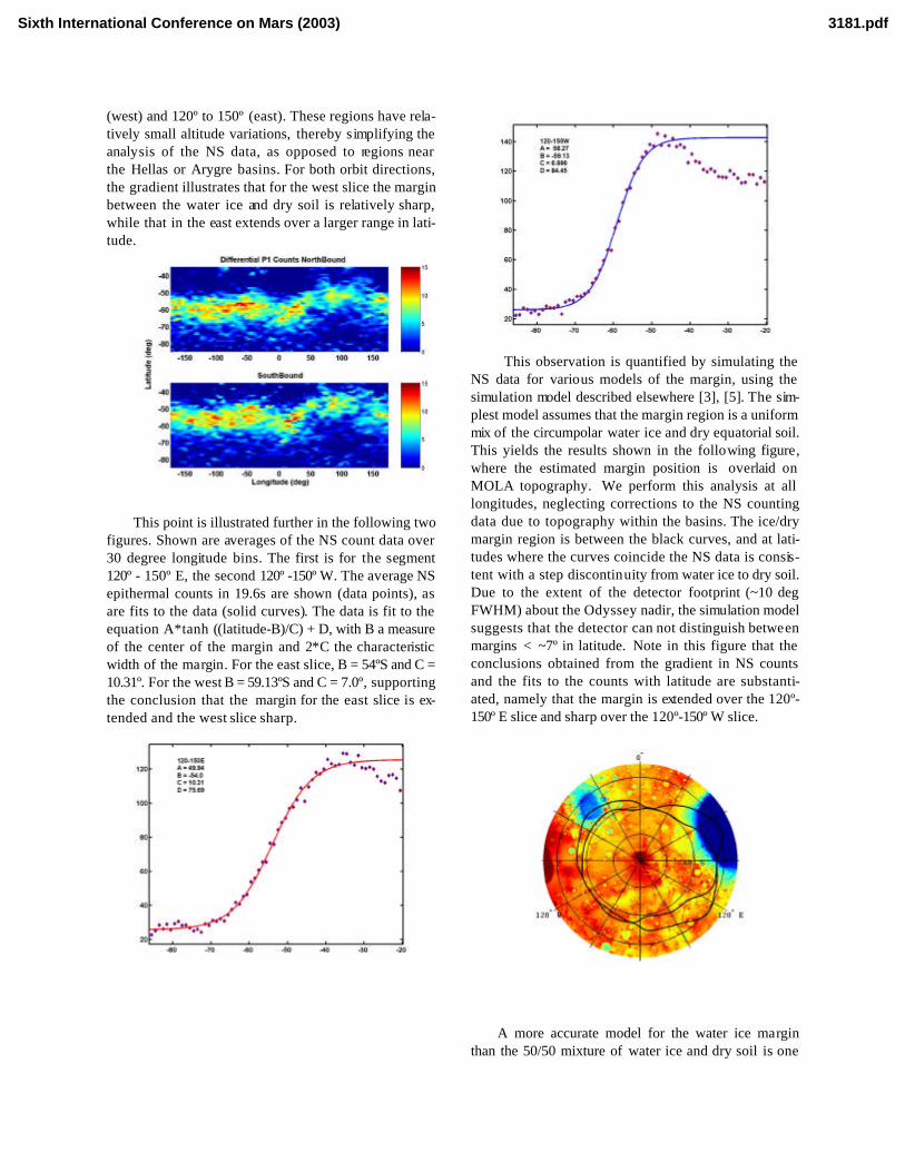
(west) and 120º to 150º (east). These regions have rela-tively small altitude variations, thereby simplifying the analysis of the NS data, as opposed to regions near the Hellas or Arygre basins. For both orbit directions, the gradient illustrates that for the west slice the margin between the water ice and dry soil is relatively sharp, while that in the east extends over a larger range in lati-tude.

This point is illustrated further in the following two

figures. Shown are averages of the NS count data over 30 degree longitude bins. The first is for the segment 120º - 150º E, the second 120º -150º W. The average NS epithermal counts in 19.6s are shown (data points), as are fits to the data (solid curves). The data is fit to the equation A*tanh ((latitude-B)/C) + D, with B a measure of the center of the margin and 2*C the characteristic width of the margin. For the east slice, B = 54ºS and C = 10.31º. For the west B = 59.13ºS and C = 7.0º, supporting the conclusion that the margin for the east slice is ex-tended and the west slice sharp.

This observation is quantified by simulating the

NS data for various models of the margin, using the simulation model described elsewhere [3], [5]. The sim-plest model assumes that the margin region is a uniform mix of the circumpolar water ice and dry equatorial soil. This yields the results shown in the following figure, where the estimated margin position is overlaid on MOLA topography. We perform this analysis at all longitudes, neglecting corrections to the NS counting data due to topography within the basins. The ice/dry margin region is between the black curves, and at lati-tudes where the curves coincide the NS data is consis-tent with a step discontinuity from water ice to dry soil. Due to the extent of the detector footprint (~10 deg FWHM) about the Odyssey nadir, the simulation model suggests that the detector can not distinguish between margins < ~7º in latitude. Note in this figure that the conclusions obtained from the gradient in NS counts and the fits to the counts with latitude are substanti-ated, namely that the margin is extended over the 120º-150º E slice and sharp over the 120º-150º W slice.

A more accurate model for the water ice margin than the 50/50 mixture of water ice and dry soil is one


where the depth of the water ice below the surface de-creases within the margin with decreasing distance from the pole. This is motivated by simulations yielding the depth to ice stability, e.g. [6]. We have performed a series of NS system simulations for margins with vari-able width in latitude; the source model in the simula-tion has three surface components, the water ice rich circumpolar mantle under a thin layer of dry dust, the margin with linearly varying ice depth that decreases in the poleward direction, and the dry soil equatorial re-gion. The simulation results for the NS counting rate variation with latitude are fit to tanh functions, as above.

The following two figures illustrate the comparison of the NS data, the MOLA 0.6 km baseline curvature data, and the NS simulation results for both the 120º - 150º W (top) and E (bottom) slices. The red curve is the normalized NS epithermal neutron counting rate and the blue curve is the bin-averaged and normalized MOLA 0.6 km curvature. The vertical dashed lines are results of the simulations, with the black dashed line the center of the margin (“B”) and the green dashed lines at B ± C degrees.

First note that, especially in the case of the sharp 120º-150º W slice at the top, the MOLA -derived curva-ture data shows the transition to the concave mantled topography almost exactly where the NS epithermal counts begin a sharp decrease. Although the details will be strengthened by further study for all longitudes and for the northern hemisphere margin, it appears that the MOLA curvature shows the concave ice mantle signature well into the NS sensed margin. Note that the margin center from the NS data is at ~59º S for the west slice and further that the uncertainty in this location is at most 1 or 2 degrees. Note that in the case of the west slice the NS can not distinguish between a step discon-tinuity and the extended margin between the green dashed lines. In the case of the east slice, again the NS counts begin to decrease almost exactly where the con-cave topography becomes more prevalent. However, the situation is more complicated both within and equa-torward of the margin. Inspection of the margin sug-gests that the signature of concave/convex curvature may be quantitatively related to the mixture of ice and dry soil regions within the NS footprint. However, both the mantling process and the underlying geology influ-ence the curvature.

References:

[1] Kreslavsky,M.H. and J.W.Head (2002)GRL,29, 10.1029/2002GL015392. [2] Mustard J.F. et al. (2001) Nature, 412,411-414. [3] Tokar R.L. et al. (2002)GRL,29, 10.1029/2002GL015691. [4] Feldman, W.C. et al., 2003, this meeting. [5] Tokar R.L. et al., GRL, submitted March,2003. [6] Mellon,M.T.and B.M.Jakosky, (1993) JGR, 98, 3345-3364.

120-150 E

120-150 W


LOW-TEMPERATURE AQUEOUS ALTERATION ON MARS: INSIGHTS FROM THE LABORATORY. N. J. Tosca, S. M. McLennan, D. H. Lindsley and M. A. A. Schoonen, Department of Geosciences, State University of New York at Stony Brook, Stony Brook, NY 11794-2100 ([email protected])

Introduction: The soil-like material mantling the

Martian surface is geologically and chemically com-plex and holds information of past and present climatic conditions on Mars. Present knowledge of this surface material suggests that low-temperature, aqueous altera-tion may have been a major factor in forming the mate-rial that has been sampled thus far by the Viking and Pathfinder landers. The term aqueous alteration used here, encompasses a wide range of processes and in-cludes both dynamic and stagnant water-rock and gas-rock alteration mechanisms. Much effort has gone into characterizing this material, and several models, based on a wide range of evidence, have given rise to many processes and resultant mineral/mineraloid phases that may be (or have been) of importance on the surface of Mars.

In terms of low-temperature aqueous alteration, the primary material being altered, that of the Martian ba-saltic crust, is somewhat constrained but the aqueous processes are not. The secondary alteration phases resulting from such processes have most likely been subject to sedimentary and physical mixing processes and as a consequence are well homogenized, some-what obscuring their chemical signatures. Therefore, it is indeed a complicated and difficult problem to ad-dress the role that low-temperature aqueous alteration may have played in the formation of the Martian soil.

One way to approach such a problem is to do so experimentally. Experimental results from aqueous alteration experiments can highlight the most impor-tant chemical processes in a given system and the rele-vance of the laboratory system to a potential model can be assessed. Some workers have taken advantage of terrestrial systems, which have been used as templates for alteration on Mars. However, new constraints on Martian surficial processes can be made by testing these models experimentally by taking advantage of the present knowledge of the primary Martian basaltic crust.

A major conclusion of this work is how, among several other factors, aqueous alteration is highly de-pendent on primary starting material. In this paper, recent results of alteration experiments with synthetic basaltic material will be evaluated and their relevance to the Martian surface will be discussed.

Low Temperature Aqueous Alteration on Mars: Several approaches to low temperature aqueous altera-tion on Mars have been taken to understand the origin

of the surface material as well as past climatic condi-tions on that planet.

The first of the major models for low temperature aqueous alteration on Mars includes palagonitization, which was first suggested by Gooding and Keil in 1978 [1]. The term palagonitization generally refers to the formation of palagonite, a hydrated, amorphous and isotropic alteration product of mafic glass [2]. The exact nature of palagonite, both chemically and miner-alogically, is poorly defined and can contain a wide range of secondary, poorly crystalline minerals, most of which are combinations of smectites [2]. The initial gel-like palagonite is metastable, and over time may evolve into crystalline products such as clays, zeolites, oxides and carbonates [2]. The precipitation of palago-nite and its associated poorly crystalline phases is de-pendent on many factors, which are important for other mechanisms of low temperature aqueous altera-tion as well and are discussed below. Palagonitization has been suggested to be important on Mars due to both the spectral similarities of palagonite material to the bright regions of Martian soils and the possibility that basaltic glass is somewhat abundant on the surface of Mars. In light of these observations, numerous stud-ies have characterized terrestrial palagonites as analogs to Martian soil [e.g., 3-5].

Another major model for low temperature aqueous alteration on Mars is the acid fog model. This model involves the interaction of volcanically derived acidic volatiles with the Martian basaltic crust [6]. These volatiles may interact with primary rock in low fluid-rock ratios, causing mineral/glass dissolution. Subse-quent evaporation of the fluid at a far-from-equilibrium state results in poorly crystalline alteration products which are composed mainly of sulfate and chloride salts. This model is proposed to have taken place in relatively recent Martian geological time (up to 1Ga) and its purpose is to explain the nature of the uppermost layer of surface material on Mars. This model was first experimentally tested in the laboratory by Banin et al. [7], who reacted Mauna Kea tephra with various acid mixtures and reported the precipita-tion of Ca and Al salts detectable by XRD. Tosca et al. [8] have further tested this model using synthesized basalt and glass with Pathfinder-derived bulk composi-tions and found that varying the starting material and aqueous conditions used in these experiments, signifi-cantly varies the secondary alteration minerals formed in this process. Figure 1 provides an example of the different alteration minerals Tosca et al. formed by


varying the primary mineralogy of the basalt. This approach and the putative alteration phases formed as a result, illustrates the importance of several different factors in low temperature aqueous alteration studies applied to Mars and will be discussed below in greater depth.

Brine interactions with the surface of Mars and their potential to form evaporites has been another suggested mechanism of alteration [9]. For example, the soluble salts found in nakhlites have been inter-preted to result from evaporitic conditions on Mars [10]. One experimental study aimed at brine interac-tion on Mars was conducted by Moore and Bullock [11], where CO2 charged water was interacted with SNC mineral mixtures for a period of one year. Model-ing evaporation of the resulting fluid predicted Ca-sulfates, Al-hydroxide and carbonates.

Studies involving the importance of weathering on the surface of Mars also include a study by McSween and Keil [12], who evaluated chemical systematics of the Pathfinder and Viking soil data. The chemical trends produced by both palagonitization and the acid fog experiments performed by Banin et al. [7] were evaluated and it was determined that the chemical trend resulting from palagonitization may provide a suitable analogy to the Martian soils. However, McSween and Keil suggest that these changes are lim-ited and that the soils contain components of different lithologies. Also, it has been suggested in this study and in others [e.g., 13] that complex sedimentary proc-

esses most likely have changed the compositions of the soils and that the homogeneous dust present on Mars may reflect the most abundant lithologies on the sur-face.

Other specific processes or secondary alteration phases, which may be important during low tempera-ture alteration, have been suggested. For example, car-bonate formation has been suggested to be important on Mars, despite little evidence for carbonates at the surface. The postulation of high partial pressures of atmospheric CO2 at one time in the past have led to the suggestion of carbonate reservoirs acting as a sink for CO2 [e.g., 14].

Sedimentary silica is another example of poten-tially important secondary alteration phases and has been suggested by McLennan [15], who notes that silica is highly mobile during basalt alteration and that secondary silica phases may have been formed and subsequently distributed in sediments. In light of this observation, McLennan suggests that this may explain some of the high silica features observed on Mars.

The origin of pre-terrestrial secondary alteration materials present in SNC meteorites has been studied experimentally by Baker et al. [16] and provides an example of basalt alteration in experimental settings. In this study, CO2, S and Cl rich waters were passed over crushed Columbia River basalt at two different temperatures, 23 and 75oC. The low temperature ex-periments formed calcite, magnesite and opal-CT. Re-sulting fluid compositions were also modeled for equi-librium evaporite assemblages.

Fig. 1 – The effect of varying primary mineralogy in basalt alteration experiments. Pathfinder soil-derived basalt (PFS) from Tosca et al. (2003) [8]. Mauna Kea Tephra from Banin et al. (1997) [7].

Laboratory Systems – Insights from Synthetic Basalt Alteration: The models discussed have several aqueous geochemical processes in common and it is important to determine what these processes are as well as the factors that govern them. Using synthetic basalts and basaltic glass of Martian composition as a starting point for aqueous alteration has begun to pro-vide important information about fundamental aqueous processes involved with basalt alteration of such a chemically unique host rock. These processes and sup-porting observations from the laboratory are discussed in this section.

Similar to how a rock is defined as an aggregate of minerals, aqueous basalt alteration can be defined as an aggregate of mineral alteration processes. The con-tributions to an aqueous system from the alteration of individual mineral/glass phases can vary significantly. Therefore, the fluid chemistry and resultant secondary minerals formed will be a direct result of the primary phases being altered. Although there are countless factors involved in aqueous environments, the discus-sion here is limited to those that are common among the major models proposed for the Martian surface. These include dissolution and its effect on fluid chem-


istry, and precipitation processes forming secondary alteration phases.

Dissolution: Interaction of basalt with fluids in most systems results first in dissolution. Dissolution is a major process in low temperature alteration, because dissolution rates and mechanisms largely determine fluid chemistry. The dissolution rates and mechanisms of mafic minerals and glasses differ significantly from each other and are dependent on several processes, including temperature, fluid composition, fluid dynam-ics and the structure of the material being dissolved. Variation of these factors has the potential to change dissolution rates by orders of magnitude. Laboratory investigations using synthetic basalt have shown that in low temperature static-fluid systems, the stoichiometry of dissolution is mainly dependent on acid concentration [8]. In systems with low pH values, dissolution proceeds stoichiometrically, releasing the components of the mineral/glass in to solution in the same proportions as the solid. As pH rises and be-comes less aggressive but still acidic, dissolution pro-ceeds non-stoichiometrically, where some components are released preferentially to others. This is the case in most natural waters on Earth and as a consequence, is a key factor in determining fluid composition.

Non-stoichiometric dissolution is controlled sig-nificantly by the crystal chemistry of the phase being dissolved. Silicate minerals dissolving non-stoichiometrically readily release ionically bonded non-structural constituents. Dissolution of orthosili-cates such as olivine liberates Fe2+, Mg2+ and H4SiO4

0 rapidly, due to the breaking of either Mg-O bonds or Fe-O bonds, which can destroy the entire structure of the mineral [17]. Under oxic conditions where Fe2+ may be oxidized to Fe3+, which is insoluble, dissolu-tion may proceed non-stoichiometrically. In frame-work silicates such as feldspars, the K+, Na+ and Ca2+ ions are released initially, while the alumino-silicate framework is hydrolyzed and destroyed at a much slower rate. The destruction of the residual framework is also dependent on the amount of Al present, as Al-O bonds are broken more easily than Si-O bonds [17]. In pyroxenes, cations occupying the M2 sites are prefer-entially released during this process. This can include Ca2+, Fe2+ and Mg2+, depending on the chemistry of the pyroxene. The residual structure of the pyroxene is then composed of M1 cations cross-linking chains of silicate tetrahedra. Destruction of the residual layer then proceeds by the breaking of M1-O bonds and Si-O bonds.

In basaltic glass, network-modifying cations such as K+, Na+, Ca2+, Mg2+, Mn2+ and Fe2+ are released preferentially to network-forming cations such as Si4+, Al3+, Ti4+ and Fe3+. Basaltic glass dissolution is de-pendent on the Si content present in the glass. Higher

Si content causes a higher degree of polymerization and therefore, decreases the rate of dissolution sub-stantially of both network-forming and modifying cations. This observation is important in that if the Type 2 terrain on Mars contains a primary high-silica glass component [18], element mobility and suscepti-bility of that primary material to chemical weathering would be significantly less. Laboratory observations have shown a decrease by a factor of 2000 in basaltic glass dissolution rate by increasing SiO2 content in the glass from 48.8 wt. % to 57.8 wt. % [19]. The non-stoichiometric release of network modifying elements forms a residual leached layer, rich in structural silica and aluminum, which is destroyed at a much slower rate.

Feldspars, pyroxenes and basaltic glass have sig-nificantly different rates of dissolution and if this dis-solution is non-stoichiometric, often form leached lay-ers at the surface, rich in residual structural silica and aluminum, which are both relatively insoluble in acidic fluids. The presence of this leached layer is therefore common with basalt alteration and may also be a common process on Mars. Upon fluid evaporation, a process common among most models of soil formation on Mars, the thickest leached layers formed in our ex-periments craze and spallate. This may be important in that the leached layers may be released in to the Mar-tian sediment and be redistributed as essentially amor-phous silica, exposing fresh mineral and glass surfaces to alter. The reactivity of such a leached layer has been documented in that the pH of pore waters in this layer have a substantially higher pH than the bulk solution, which is conducive to precipitation of secondary phases inside the depleted layer [20]. Also, it may eas-ily acquire negative surface charge and cause adsorp-tion of aqueous constituents on to this layer [20]. Fi-nally, the leached layer may also recombine and po-lymerize to form small amounts of phases such as clays, if enough aqueous constituents are available in the fluid [20].

Controls on fluid chemistry: Using basaltic compo-sitions relevant to Mars, we observe that primary min-eral phases each control different aspects of fluid chemistry. For example, Na+, K+ and Ca2+ are ubiqui-tous in initial fluid compositions, due to their soluble nature and their weaker bonding in feldspars, pyrox-enes and basaltic glass. The chemistry of Mg in these fluids is more complex. For example, forsteritic oli-vine is observed to dissolve the quickest in synthetic basalt alteration experiments, releasing large amounts Mg2+ and H4SiO4

0 into solution. This in turn raises the state of saturation with respect to amorphous silica as well as Mg-SO4 phases, if fluids are rich in SO4

2-. Magnesium from pyroxenes, however, may be re-leased but kinetically inhibited, due to its preferential


M1 site occupancy and stronger bonding characteris-tics. Magnesium rich pyroxenes, such as enstatite, may be able to release significant amounts of Mg from the M2 site. This release is most likely limited to the first stages of alteration, in that a silica-rich depleted layer may soon form to retard dissolution. Therefore, in ki-netically restricted models of alteration, olivine may be controlling the Mg2+ in the fluid as opposed to pyrox-enes. Ferrous iron may also behave in this way, but results from synthetic basalt alteration experiments show that Fe2+ release from pyroxenes is much more significant than Mg2+ release in initial stages of altera-tion. With large amounts of Fe2+ being released into solution from pyroxenes and olivine, the fate of Fe2+ in solution remains uncertain because Fe2+ oxidation mechanisms are unconstrained. There are several pathways by which Fe2+ could be oxidized and in our synthetic alteration experiments exposed to the Earth’s atmosphere, oxygen is the most important oxidant, producing secondary ferric phases as grains and coat-ings. More studies remain to be done to determine po-tential oxidants of Fe2+ on the Martian surface. Solid state iron oxidation of ferrous silicates and oxides [21] remains another possible mechanism for production of secondary ferric phases on Mars, but has been largely unexplored in this context.

Precipitation: The precipitation of minerals from various fluids depends on several factors. Among the most important factors observed in our experiments are the saturation state of the alteration mineral and the structure of both the precipitating mineral as well as the substrate on which it precipitates. Several experi-ments performed with synthetic basalt have shown large amounts of poorly crystalline alteration minerals precipitating on the surfaces of minerals and glasses. The initial phases are metastable or amorphous phases, which most likely have a higher rate of nucleation than subsequent stable phases, due to their wide-spread occurrence and poor crystallinity [22]. This process is referred to as Ostwald ripening and models such as palagonitization are dependent on such a process [2]. For example, the initial alteration phases precipitated during the formation of palagonite will most likely be metastable with respect to common alteration materials such as smectites observed in more advanced aging of palagonite.

Conclusions: Models for formation of the Martian soil share common fundamental aqueous processes, which are dependent on several factors prevailing on the surface. It is important to understand what these processes are and how they may be important during low temperature aqueous alteration. Several of these alteration processes begin with dissolution of primary mineral phases and are dependent on the chemistry of

the minerals themselves. Therefore, when testing mod-els of low temperature aqueous alteration on Mars, relevant starting material is one of the most important factors. A wide variety of robust, analytical resources are also needed to characterize the chemical processes operating in laboratory systems, because microscopic observations in many cases, have global implications.

The discussion presented here is the result of the first stage of a large-scale approach to understanding the surficial processes on Mars experimentally. Many questions have been raised in light of recent observa-tions and therefore, much work is needed to place fur-ther constraints on the origin of the Martian soil. More models for soil formation will be tested using even more starting materials, aqueous environments and experimental and analytical methods. The capability of synthesizing compositionally accurate starting material as well as adjusting experimental and analytical meth-ods accordingly will result in observations aimed at a wide variety of microscale and macroscale processes that may be of importance for the surface of Mars. New constraints from future missions of Martian ex-ploration will be used in our approach in further refin-ing our understanding of the Martian surface material.

References: [1] Gooding, J.L. and Keil, K. (1978) Geophys. Res. Lett., 5, 727-730. [2] Stroncik, N.A. and Schmincke, H.-U. (2002) Int. J. Earth Sci., 91, 680-697. [3] Morris, R.V. et al. (2000) J. Geophys. Res., 105, 1,757-1,817. [4] Morris, R.V. et al., (2003) LPS XXXIV, Abstract #1874. [5] Bell, J.F. et al. (1993) J. Geophys. Res., 98, 3,373-3,385. [6] Banin, A. (1996) Adv. Space Res., 18, 233-240. [7] Banin, A. et al. (1997) J. Geophys. Res., 102, 13,341-13,356. [8] To-sca, N.J. et al. (2003) LPS XXXIV, Abstract #1325. [9] Bridges, J.C. and Catling, D.C. (2001) Space Sci. Rev., 96, 365-392. [10] Bridges, J.C. and Grady, M.M. (1999) Met. Planet. Sci., 34, 407-415. [11] Moore, J.M. and Bullock, M.A. (1999) J. Geophys. Res., 104, 21,925-21,934. [12] McSween, H.Y. Jr. and Keil, K. (2000) Geochim. Cosmochim. Acta, 64, 2155-2166. [13] McLennan, S.M. (2000) Geophys. Res. Lett., 27, 1,335-1,338. [14] Morse, J.W. and Marion, G.M. (1999) Am. J. Sci., 299, 738-761. [15] McLennan, S.M. (2003) Geology, 31, 315-318. [16] Baker, L.L. et al. (2000) Met. Planet. Sci., 35, 31-38. [17] Oelkers, E.H. (2001) Geochim. Cosmochim. Acta, 65, 3,703-3,719. [18] Bandfield, J.L. et al. (2000) Science, 287, 1,626-1,630. [19] Tosca, unpublished data. [20] Casey, W.H. and Bunker, B. (1990) Rev. Mineral. Geochem., 23, 397-426. [21] White, A.F. (1990) Rev. Mineral. Geochem., 23, 467-509. [22] Stumm, W. and Morgan, J.J. (1996) Aquatic Chemistry, Wiley, 1,022 p.


THE BEAGLE 2 ENVIRONMENTAL SENSORS: INTENDED MEASUREMENTS AND SCIENTIFICGOALS. M. C. Towner1, T. J. Ringrose 1, M. R. Patel1, D. Pullan2, M. R. Sims2, S. Haapanala3, A.-M. Harri3, J.Polkko3, C. F. Wilson3 J. C. Zarnecki1, 1 PSSRI, Open University, Walton Hall, Milton Keynes, UK,[email protected], 2 Space Research Centre, Dept of Physics and Astronomy, University of Leicester, Univer-sity Road, Leicester, UK, 3 Finnish Meteorological Institute, Geophysical Research Division, P.O. BOX 503, FIN-00101 Helsinki, Finland, 4 Atmospheric, Oceanic and Planetary Physics, Clarendon Laboratory, University of Ox-ford, Parks Road, Oxford, U.K.

Summary: Beagle 2 is a 30kg lander for Mars, op-timized for exobiology, launching in June 2003 as partof the European Space Agency (ESA) Mars Expressmission[1]. The expected lifetime on the surface is 180sols, with a landing site in Isidis Planitia[2]. One of theinstruments on board is a suite of sensors for monitor-ing the local environment, and hence helping to deter-mine if life could, or still can, exist there. The suiteconsists seven sensor subsystems weighing 153 grams,and due to the tight constraints of the Beagle 2 lander,primarily of simple analogue sensors, distributed overthe lander. The suite has 2 major themes:

A meteorological package will record wind speedand direction, atmospheric pressure and temperature ata variety of heights, and look for particle saltation.

A life environment subsystem will measure the lo-cal radiation environment, the surface UV flux, andattempt to verify the presence of oxidants such as hy-drogen peroxide, (without identifying the particularspecies present). Additional sensors will record theupper atmosphere density profile (determined by theacceleration encountered during probe entry and de-scent).

Introduction: Measurements of the local environ-mental conditions on Mars are a valuable tool as partof a lander’s repertoire - both as independent meas-urements in their own right (for example meteorology),or providing context information which adds to thevalue of data from specific instruments (for examplelocal temperature). The Beagle 2 lander, part of theMars Express mission to Mars includes an array ofsensors, designated the Environmental Sensors Suite(ESS), designed to monitor various local conditions.The sensors are designed to answer specific sciencegoals, as well as providing support for the other on-board instruments.

Instrument description: The ESA Mars Expressmission is due for launch in late May or early June2003, arriving at Mars on 26th December 2003, initiallybraking into an elliptical orbit, 250km by 11,580km[1]. If all goes well, it will be at Mars at the same timeas the ISAS spacecraft Nozomi and the NASA MarsExploration Rovers, Mars Odyssey (and possibly MarsGlobal Surveyor if still active). The Mars Express sci-entific payload is described by Schmidt et al. [1]. The

Beagle 2 lander is due to land in the Isidis Basin, at270oW and 10.5oN [2]. It has a landed mass of 30kg,and uses an airbag and parachute system for descent,with an intended primary mission lifetime of 180 solson the surface.

Onboard Beagle 2, ESS will operate throughout themission lifetime and is intended to study both short(seconds, minutes, days) and long term (seasonal)timescale variations in the local environment. It has 2major themes:

1) Landing site meteorology, A major sciencegoal of the meteorology program is to improve ourunderstanding of the Martian dust cycle. High-frequency measurements will be used to characterizenear-surface turbulence, and to make quantitativemeasurements of dust devils (convective vortices).These high-frequency measurements of potentiallydust-raising winds are supplemented with a sensorwhich will estimate the momentum of saltated particles.Low-frequency meteorological measurements will pro-vide a long-term meteorological record, enabling studyof day-to-day and seasonal variation in weather pat-terns.

2) The astrobiological implications of the localradiation and oxidative environment. Since the majorBeagle 2 payload instrument, GAP provides a compre-hensive analysis of the chemical locale, it was decidedto concentrate on the astrobiological factors that wouldnot be seen by GAP - the oxidising properties of thenear surface environment (such knowledge is also un-likely to be recovered easily by any future sample re-turn mission). As such ESS attempts to quantify theexistence of a local oxidising condition, oxidant pro-duction and transport. ESS investigates the local UVenvironment, to quantify a possible production mecha-nism [3], and measures the dust saltation rates (and theairborne dust loading via the camera) - a possibletransport (storage) mechanism. Monitoring a simple insitu deposited silver film allows ESS to detect andquantify the oxidising capability of the air and regolith.One final astrobiological experiment, unrelated to oxi-dants, is the measurement of the total radiation doseover the mission lifetime. This characterization of thesurface environment will also aid in the issue of thepossibility of sub-surface life. Knowing the UV flux atthe surface, it is possible to quantify UV penetration


into the regolith, especially when combined with sur-face analysis and imaging through the various instru-ments on Beagle 2.

Resources on the Beagle 2 lander are particularlyscarce [6]. This has driven the overall mass budget forthe seven chosen sensors of 153 grams. In some casesthis has forced a move away from solutions based ondesigns with previous spaceflight heritage, in favour ofcommercial microtechnology-based solutions whichare likely to have a higher associated risk of failure.However, this is compatible with the philosophy of theentire Beagle 2 design where cost and mass constraintshave required an acceptance of risk throughout, in-cluding elimination of complete redundancy for mis-sion critical systems.

Meteorology sub-system: Wind sensor This sensoris mounted on end of the robotic arm, such that it canbe positioned at different heights and orientations. It isa hot film sensor, similar in concept to Viking andpathfinder instruments. It has been calibrated from 0-30m/s, although it will measure higher and furtherground calibration remains to be done. Direction ismeasured to within to 10o.

Temperature sensor Air temperature is measured at2 heights. One sensor is incoporated intop the windsensor, on the arm, , and the second is located on theedge of one of the solar panel sheets, to minimize inter-ference from the probe body. Expected absolute accu-racy is 0.1K, with a resolution of 0.05K. Simultaneousmeasurements of temperature at two different heightscan be used to estimate a vertical thermal profile.

Pressure Sensor This sensor is profvided by theFinnish Meteorological Institute, based on a capacitivediaphragm design as flown on Mars-96. It has a rangeof 0-30mBar, with an absolute accuracy of 200�Barand a resolution of 2�Bar.

Life environment sub-system: Radiation sensorThis sensor is a RadFET, and provides a cumulativeradiation dose information on the flux of high energycosmic rays and solar protons at the Martian surface.

UV sensor Short wavelength UV, such as UVB andC are harmful to life, and can directly damage DNA.The UV environment on Mars is known to be harsh,and it is unlikely that life can survive on the surface,but subsurface life may still be possible. This sensor isa simple array of upward looking photodiodes withappropriate band-pass filters, giving a 5 point spectrumfrom 200-400nm. A 6th channel has no filter and pro-vides aging information.

Wavelength(nm)

Comment

210 Main TiO2 dust absorption band230 Biologically damaging and rapidly

time varying regime250 Secondary TiO2 band300 Mid UVB350 Mid UVA

Open channelTable 1, detailing the UV sensor channels

Oxide sensor One controversial issue arising fromthe results from the Viking landers is the postulatedpresence of hydrogen peroxide (H2O2) or other oxi-dizing compounds in the soil, used in several cases toexplain the results of the experiments designed to de-tect Martian life. This sensor deploys a thin silver filmin situ by pulsed evaporation of a silver bead, andmonitors the resistance of the film with time as it oxi-dizes. By repeated evaporations at different times ofday, in conjunction with input from the cameras, theUV sensor and the onboard microscope, useful infor-mation will be obtained about the ‘life cycle’ of anyoxidants present.

Additional sensors: Dust impact sensor Impactsfrom dust in the atmosphere of Mars will help to indi-cate how material is moved over the planet's surface.The sensor is a simple 50x50mm Al sheet, 0.25mmthick, with a piezoelectric film on the rear face. Mini-mum sensitivity is around 1x10-6 kgms-1

Accelerometer Measurements of deceleration of theprobe during the atmospheric entry and landing se-quence can be used (in combination with the drag coef-ficient for the heat shield) to derive the upper atmos-phere density and pressure. See for example Withers etal [7].

Two single axis sensors are used, with rangesof±30g and ±10g on the probe axis. During the earlyentry phases pressure and density can be derived inupper atmosphere with an initial vertical resolution of150m. Horizontal wind-speeds will be monitored dur-ing later descent after chute deployment, and the probetilt once at rest will also be recorded.

Measurement Strategy: Throughout the surface-mission lifetime, each sensor will be sampled at a lowrate, typically taking one reading from each sensorevery 30 minutes. In addition to this, to study quicklychanging conditions such as the dust devils seen byViking[8] and Mars Pathfinder[9], the wind, tempera-ture, pressure, and dust sensors will have ahigh sam-pling rate mode (1 per second), whereby data from theprevious 5 minutes is buffered and onlyreturned toearth (along with a further 5 minutes of data) should


any transient effects be detected. Of particular interestare dust devils, which may be the primary source ofdust movement on Mars, and responsible for the ho-mogeneity of the dust measured at the Viking and Path-finder sites.

References: [1] R Schmidt et al, ESA Bulletin-European Space Agency, 1999, No.98, pp.56-66 [2] JCBridges et al, JGR , 108 (E1): 5001, 2003 [3] AP Zentand C McKay, Icarus, 108, 146-157, 1994 [6] J Clem-met, ESA SP-468, 9-14, 2001 [7] P Withers et al,Planetary and Space Science, submitted. [8] For exam-ple, PP Thomas and P Gierasch, Science 230, 175-177,1985. [9] JT Schofield, JR Barnes, D Crisp, RMHaberle, S Larsen, JA Magalhaes, JR Murphy, A Seiff,G Wilson, Science 278, 1752-1758, 1997


CONVECTIVE PLUMES AS ‘COLUMNS OF LIFE’. B. J. Travis, Los Alamos National Laboratory (EES-2/MS-T003, LANL, Los Alamos NM 87545; [email protected] ).

Introduction: A great deal of evidence supports thestatement that water was abundant on Mars in its earlyhistory and that much of that inventory still exists to-day as ice and permafrost in the sub-surface, verylikely with liquid water below that [1], [2]. A recentstudy [3] suggests that liquid water will be subject towidespread hydrothermal convection driven by thegeothermal gradient, or the geothermal gradient aug-mented by magmatic intrusions. Subsurface convec-tive flow patterns for Mars conditions are of the rolland plume types, with warm, upwelling plumes melt-ing through the permafrost region and approachingcloser to the surface and exhibiting higher upward flowrates than rolls (see Fig. 1). Water temperatures withinupwelling plumes can range from 40 – 100 oC, at theirbase, to 0 – 10 oC at their top (even colder for salinesolutions), depending on local heat flux and perme-ability structure of the host rock (see Fig. 2). Theseconvective patterns are stable and long-lasting, andcould provide a potential habitat for microbial life bybringing nutrients to and through microbial communi-ties living in subsurface soil and rock. Upwellingplumes could function as ‘columns of life’. Further,for the higher geothermal heat fluxes of the past, flowwill be episodic, characterized by occasional periods ofenhanced flow rates and re-organization of the spatialarrangement of plumes, possibly providing a stimulusfor evolution. Fisk & Giovannoni [4] argue, based on the diversityof electron donor-acceptor mechanisms that microbiallife on Earth has developed and on the similaritiesbetween the chemical and mineralogical make-up ofEarth and Mars, that many chemolitho-autotrophic mi-crobes that inhabit the Earth’s seafloor could likelysurvive in the Martian subsurface. Likely microbialcandidates would include anaerobic thermophiles thatutilize sulfur and carbon dioxide and iron, examples ofwhich are found in abundance within mid-ocean ridgevent systems. Microbes in Mid-Ocean Ridge Systems as Exam-ples. In hydrothermal vents at mid-ocean ridges andother vent fields, there are many examples of microbes(mesothermophiles and hyperthermophiles) that utilizeaerobic and anaerobic chemolithotrophic energysources [5], typically in the temperature range 70 - 110oC. These rely primarily on sulfur and hydrogenchemistry. There is evidence for interactions betweenthermophilic species. There are also examples of mi-crobes (cryophiles) that can live in briny water inclu-sions in ice. Some Anaerobic Energetic Reactions. Commonreactions that provide energy for anaerobic thermo-philic microbial metabolism on Earth include:

Sulfate reduction (e.g., Archaeoglobus profundus, at90 oC)

Methanogenesis (e.g., Methanococcus igneus, at 86oC)

Denitrification (e.g., Pyrobaculum sp., at 103 oC)

Another possible source of energy: pyrite formation

Simple Monod Model for Microbial Metabolism.For a simple stoichiometry of the form

and assuming Monod (enzyme) kinetics for metabolicreactions, the following set of governing equations ap-proximate transport, diffusion and reaction in the sub-surface:

where A represents an electron donor (e.g., CH4, H2,H2S ), B is an electron acceptor (e.g., O2, S, SO4, NO3,CO2), M represents microbial biomass, Ki equals half-saturation and k equals max. utilization rate, V isDarcy velocity, e is porosity, Di equals diffusivity, kd isdeath rate of microbes. Estimate of Growth Potential. Numerical solu-tions of the above equation set in general two and threedimensional settings, with even more complex meta-bolic models, are available [6]. Here, estimates of so-lutions will suffice. Making a steady state assumption,and assuming that B is in excess (B >> KB), neglectingdiffusion and assuming locally uniform flow, A = KA

c / (1 - c), and c = kd / (b k), which implies that

M ~ (QA/L)/(c k) = V [A]in b/ (e L kd)

where [A]in is the concentration of electron donor influid being entrained into a plume. Typical ranges of

A + aB Æ bM + byproducts

∂A∂t = - k M A

KA + A BKB + B - 1e—⋅(VA) + DA—2A

∂B∂t = - ak M A

KA + A BKB + B - 1e—⋅(VB) + DB—2B

∂M∂t = bk M A

KA + A BKB + B - kdM

CO2 + 6H2 + SO4-2 Æ [CH2O] + S-2 + 5H2O

2CO2 + 6H2 Æ [CH2O] + CH4 + 3H2O

CO2 + 8H2 + 2NO3- Æ [CH2O] + N2 + 7H2O

FeS + H2Saq Æ FeS2 + H2

CO2 + H2 Æ HCOOHFeS + H2Saq + CO2 Æ FeS2 + H2O + HCOOH


COLUMNS OF LIFE: B. J. Travis

values for the various coefficients for Earth-based mi-crobes are: b = 0.33 - 0.50, KA ~ O([A]in), kd ~ 10-4 -10-1 /day, e ~ 0.01 - 0.30, k ~ 10-2 - 10/day. Represen-tative flow rate V in rolls and plumes for hypotheticalhydrothermal convection on Mars [6] ranges from2x10-4 - 6.5x10-3 m/day. This yields the estimates:M ~ 10-2 [A]in/L for weak convection (rolls), and

short-lived microbesM ~ 102 [A]in/L for strong convection (plumes),

hardy microbesIf [A]in ~ 10-5 g/cc and L ~ 1,000 m, then M ~ 10-6 g/ccwhich converts to about 106 microbes/cc in a plume. Conclusions: Regions of warm to hot water shouldexist in the Martian subsurface (40-100 oC). Thelower-lying northern plains are a more likely place forthe fully saturated flow model assumed here, but if theH2O inventory is sufficiently large, then the modelmay be applicable to parts of the southern hemisphereas well. Warm, flowing water in long-lasting upwell-ing plumes and convective rolls is capable of carryingdissolved minerals continuously to and through anymicrobial communities living within a hydrothermalconvection system. Estimates of metabolic rates vstransport rates suggest that microbial life at concentra-tion levels up to 10-6 g/cc (106 microbes/cc) might besustainable over a spatial interval of 1,000 meters.Temperature structure within plumes provides a rangeof temperature zones and the chemical make-up couldallow a series of life zones, ranging from habitationsfor thermophiles deep in the regolith at the base ofplumes to mesophiles in the middle regions tocryophiles at plume tops. If plumes breached the sur-face occasionally, there could have been biomass resi-due deposited on the surface. There is also the possi-bility of seeps of very low concentrations of by-product gases such as methane. Numerical simulation of convective patterns with rea-sonable values of controlling parameters such as geo-thermal heat flux and permeability structure and solu-bilities of various compounds, allows estimation of themaximum rate at which required substrates and nutri-ents could be delivered to any microbial communitiesliving within convective plumes. When coupled to mi-crobial metabolic models, these reactive transportsimulations can provide an estimate of the possiblesize and spatial distribution of such communities.

References: [1] Clifford, S.M. (1993) JGR 98,10973-11016. [2] Clifford, S.M. and T.J. Parker (2001)Icarus 154, 40-79. [3] Travis, B.J., N.D. Rosenberg,J.N. Cuzzi, in press, JGR-Planets. [4] Fisk, M.R. &S.J. Giovannoni (1999) JGR 104, 11805-11815. [5]Jannasch, H. W. (1995) in Seafloor HydrothermalSystems AGU Monograph 91, 273-296. [6] Travis,B.J., N.D. Rosenberg (1997) Environ. Sci & Tech. 31,3093-3102.

Figure 1. An example of pure-water subsurfacehydrothermal convection under Mars-like conditions.Sides of box are 10 km each (vertical not to scale).Surface shown is the interface between underlying liq-uid water and overlying frozen soil, i.e., the 0 oC iso-therm. The interface reflects the underlying regions ofconvective motion. The label ‘500 darcy’ refers to sur-face value of permeability; permeability and porositydecrease exponentially from the surface down. Surfacetemperature is – 60 oC and heat flux at the bottom is 40mW/m2.

Figure 2. Temperature structure within hydrothermalconvection plumes and rolls in the subsurface. Bluesurface is the 10 oC isotherm, Green is 20 oC, andchartreuse is 30 oC. The box region is 10 km on a side.Basement temperatures can range from 40 to 100 oCdepending on vigor of convection. Closeness of plumetop to surface depends in part on salt content.


Contents — T - lpi.usra.edu · MGS TES data over the poles are taken much more frequently than...

Documents

Transcript of Contents — T - lpi.usra.edu · MGS TES data over the poles are taken much more frequently than...