Container Line Supply Chain Security Analysis under ...
305
Container Line Supply Chain Security Analysis under Complex and Uncertain Environment A Thesis submitted to the University of Manchester for the degree of Doctor of Philosophy In the Faculty of Humanities 2011 DAWEI TANG Faculty of Humanities
Transcript of Container Line Supply Chain Security Analysis under ...

Container Line Supply Chain Security Analysis under Complex
and Uncertain Environment
A Thesis submitted to the University of Manchester for the degree of
Doctor of Philosophy
In the Faculty of Humanities
2011
DAWEI TANG
Faculty of Humanities

2
Contents
Contents ............................................................................................................. 2
List of Figure ....................................................................................................... 7
List of Table ........................................................................................................ 8
Abbreviations .................................................................................................... 10
Abstract ............................................................................................................. 12
Declaration ........................................................................................................ 15
Copyright Statement ......................................................................................... 16
Acknowledgement ............................................................................................. 17
1 Chapter 1 Introduction ............................................................................... 19
Abstract ......................................................................................................... 19
1.1 Background .......................................................................................... 19
1.2 Research questions ............................................................................. 22
1.3 Research aims and objectives ............................................................. 23
1.4 Research methodology ........................................................................ 24
1.5 Research originations and beneficiaries .............................................. 26
1.6 Structure of the thesis .......................................................................... 29
1.7 Conclusion ........................................................................................... 34
2 Chapter 2 Literature Review ...................................................................... 36
Abstract ......................................................................................................... 36
2.1 Introduction .......................................................................................... 36
2.2 Research on CLSC security ................................................................. 37
2.2.1 Basic definitions ............................................................................ 37
2.2.2 Research on security issues in CLSC from a general level ........... 38
2.2.3 Research on specific issues of security in CLSC .......................... 42
2.3 Research on risk analysis methods with their application in the areas
relevant to CLSC security assessment .......................................................... 47
2.4 Research on resource allocation in response to security and safety
incidents ........................................................................................................ 51
2.5 Research on existing methods for information aggregation for Multi
Criteria Decision Analysis problems .............................................................. 54
3
2.6 Summary and limitations of current literature relevant to the research in
this thesis ...................................................................................................... 58
2.7 Requirements on research for security analysis in CLSC .................... 58
2.8 Conclusion ........................................................................................... 60
3 Chapter 3 Models for CLSC security assessment ..................................... 62
Abstract ......................................................................................................... 62
3.1 Introduction .......................................................................................... 62
3.2 General model for overall security assessment in CLSC ..................... 62
3.2.1 Physical flow of CLSC and security assessment model for CLSC 63
3.2.2 Security representation and factors measurement ........................ 66
3.3 Model for security assessment of a port storage area in a CLSC against
cargo theft ..................................................................................................... 70
3.3.1 The hierarchical model .................................................................. 70
3.3.2 Measurement of factors in the security assessment model in
Appendix 1 ................................................................................................. 75
3.4 Case study ........................................................................................... 78
3.4.1 Case background .......................................................................... 78
3.4.2 Measurement of factors according to real information collected ... 79
3.5 Conclusion ........................................................................................... 80
4 Chapter 4 Generation of belief degrees in Belief Rule Bases and security
assessment of CLSC using RIMER .................................................................. 82
Abstract ......................................................................................................... 82
4.1 Introduction .......................................................................................... 82
4.2 Introduction of Belief Rule Base and generation of belief degrees in
Belief Rule Bases .......................................................................................... 83
4.2.1 Introduction to Belief Rule Base .................................................... 83
4.2.2 A brief introduction to Bayesian Network ....................................... 85
4.2.3 Relationship between Belief Rule Base and Bayesian Network .... 86
4.2.4 Generation of belief degrees in BRBs ........................................... 88
4.3 A brief introduction inference scheme of RIMER ................................. 93
4.3.1 The ER approach .......................................................................... 94
4.3.2 Input information............................................................................ 96
4.3.3 Rule activation ............................................................................... 97
4.3.4 Inference of RIMER ....................................................................... 98
4
4.4 Case study ........................................................................................... 98
4.4.1 Generation of belief degrees in BRBs in the security assessment
model in Appendix 1 .................................................................................. 99
4.4.2 Assessment of security level of port storage areas along CLSCs
against cargo theft ................................................................................... 104
4.5 Conclusion ......................................................................................... 109
5 Chapter 5 Assessment based resource allocation to improve security in
CLSC .............................................................................................................. 111
Abstract ....................................................................................................... 111
5.1 Introduction ........................................................................................ 111
5.2 Sensitivity analysis of RIMER ............................................................ 112
5.2.1 Basis of sensitivity analysis ......................................................... 112
5.2.2 Process of sensitivity analysis ..................................................... 113
5.3 Optimal resource allocation based on sensitivity analysis ................. 115
5.3.1 The relation between C and ijα∆ ................................................. 116
5.3.2 The relation between ijα∆ and DU∆ ............................................. 117
5.3.3 Maximize security improvement under the constraint on budget . 118
5.3.4 Minimize cost under the requirement on security improvement .. 119
5.4 Case study ......................................................................................... 119
5.5 Conclusion ......................................................................................... 129
6 Chapter 6 Handling Different Information Aggregation Patterns for Security
Assessment of CLSC ...................................................................................... 131
Abstract ....................................................................................................... 131
6.1 Introduction ........................................................................................ 131
6.2 Different aggregation patterns in security assessment model ............ 132
6.2.1 Aggregate information under heterogeneous pattern .................. 137
6.2.2 Aggregate information under homogeneous pattern ................... 138
6.3 Methods to handle different information aggregation patterns under the
framework of RIMER ................................................................................... 142
6.3.1 Handling heterogeneous aggregation pattern and homogeneous
aggregation pattern .................................................................................. 142
6.3.2 Handling aggregation pattern with EIF(s), VIF(s) and BF(s) ........ 144
6.4 Case study ......................................................................................... 147

5
6.4.1 Heterogeneous information aggregation ..................................... 147
6.4.2 Homogeneous information aggregation ...................................... 148
6.4.3 Information aggregation with EIF(s) involved .............................. 152
6.4.4 Information aggregation with VIF(s) involved .............................. 155
6.4.5 Information aggregation with the coexistence of EIF and BF ...... 157
6.4.6 Assessment of security against cargo theft in port storage area
based on real data collected .................................................................... 159
6.5 Conclusion ......................................................................................... 161
7 Chapter 7 Handling Different Kinds of Incomplete Information for Security
Assessment of CLSC ...................................................................................... 164
Abstract ....................................................................................................... 164
7.1 Introduction ........................................................................................ 164
7.2 Different sources of incompleteness and different categories of
incompleteness ........................................................................................... 165
7.3 Limitations of RIMER in handling incomplete information .................. 168
7.3.1 Current scheme to handle incompleteness in RIMER ................. 168
7.3.2 Limitations of RIMER in handling incompleteness....................... 170
7.4 A new method to handle incompleteness based on RIMER .............. 171
7.4.1 Representation of both local and global incompleteness ............ 171
7.4.2 Generation of interval belief degrees in BRBs ............................. 173
7.4.3 The inference based on RIMER .................................................. 179
7.4.4 Summary ..................................................................................... 183
7.5 Case Study ........................................................................................ 183
7.5.1 Incompleteness regarding input information of the security
assessment model ................................................................................... 184
7.5.2 Incompleteness regarding the relation among antecedents and
consequence in BRBs in the security assessment model ........................ 186
7.5.3 Inference under incomplete information ...................................... 190
7.5.4 Summary of security assessment result of all 5 ports ................. 193
7.6 Conclusion ......................................................................................... 196
8 Chapter 8 Conclusion .............................................................................. 198
Abstract ....................................................................................................... 198
8.1 Summary of the thesis ....................................................................... 198
8.2 Contribution of the research in the thesis........................................... 202

6
8.3 Limitations of the research in the thesis ............................................. 205
8.4 Directions of future research .............................................................. 207
References...................................................................................................... 209
Appendix 1 Hierarchical model for security assessment against cargo theft of
a port storage area along a CLSC .................................................................. 227
Appendix 2 Grades/referential values and corresponding meanings to
describe basic factors in Appendix 1 ............................................................... 232
Appendix 3 Grades/values for the non-basic factors in Appendix 1 ........... 243
Appendix 4 Questionnaire to collect information from PFSOs .................... 245
Appendix 5 Belief Rule Bases in the security assessment model in Appendix
1 without the consideration of different information aggregation patterns ....... 254
Appendix 6 Different aggregation pattern existing in the security assessment
model in Table A1 ........................................................................................... 277
Appendix 7 Belief Rule Bases for the security assessment model in Appendix
1 with a homogeneous information aggregation pattern ................................. 288
Appendix 8 Publications Relevant to the Thesis ......................................... 305
7
List of Figure
Figure 1.1 Structure of the thesis ...................................................................... 34
Figure 2.1 Effective area of CSI, C-TPAT and ISPS Code ............................... 41
Figure 3.1 A typical voyage of a container along a CLSC ................................. 63
Figure 3.2 High Level Security assessment model of a CLSC with port of origin
as an example stage ......................................................................................... 65
Figure 3.3 Framework to model security in a basic unit for CLSC security
assessment ....................................................................................................... 68
Figure 3.4 Skeleton of the model for security assessment against cargo theft of
a port storage area along a CLSC .................................................................... 75
Figure 4.1 A basic BN fragment ........................................................................ 86
Figure 7.1 Assessment framework with M levels ............................................ 182

8
List of Table
Table 1.1 Research methodologies categorized by research objectives .......... 26
Table 4.1 Pair-wise comparison matrix to generate ( )ji j jpP D D A A= = ........... 92
Table 4.2 Random Index ................................................................................... 93
Table 4.3 Pair-wise comparison matrix to generate ( )P LF LCA when LCA M=
........................................................................................................................ 100
Table 4.4 The probabilities of LF conditional on LCA’s different states ........... 100
Table 4.5 The probabilities of LF conditional on LCO’s different states .......... 100
Table 4.6 Probabilities of LF conditional on different state combinations of LCO
and LCA .......................................................................................................... 102
Table 4.7 Initial BRB for relation among LCO, LCA and the performance of LF
........................................................................................................................ 102
Table 4.8 Revised BRB for relation among LCO, LCA and the performance of
LF .................................................................................................................... 103
Table 4.9 Security Assessment Results for different ports in the UK and China
........................................................................................................................ 108
Table 5.1 Grades/referential values for Coverage, Capability and Robustness of
an access control system and their meanings ................................................ 121
Table 6.1 Pair-wise comparison table to generate P(PM|MM) when MM=E ... 149
Table 6.2 BRB for the relation among MM, OM and PM ................................. 151
Table 6.3 Security assessment result generated by Unique Aggregation Pattern
and Multiple Aggregation Pattern .................................................................... 160
Table 7.1 Interval valued pair-wise comparison matrix for BRB generation .... 174
Table 7.2 Probability interval of D being described by its referential values on
the condition that iA takes different referential values ..................................... 177
Table 7.3 Pair-wise comparison matrix for impact of Capability on Alarm System
when Capability is ‘High’ ................................................................................. 186
Table 7.4 Consistency check for pair-wise comparison matrix in Table 7.3 .... 187
Table 7.5 BRB for Performance of Alarm System based on incomplete
knowledge ....................................................................................................... 190

9
Table 7.6 Security assessment results for the 5 ports using different methods
........................................................................................................................ 194
Table 7.7 Summary of utility interval width for different ports under different
methods .......................................................................................................... 194
10
Abbreviations
AEO: Authorised Economic Operator
ANN: Artificial Neural Network
BF: Base Factor
BN: Bayesian Network
BRB: Belief Rule Base
CBP: Customs and Border Protection
CLSC: Container Line Supply Chain
CPT: Conditional Probability Table
CSI: Container Security Initiative
C-TPAT: Customs-Trade Partnership Against Terrorism
DAG: Directed Acyclic Graph
DHS: Department of Homeland Security
DSS: Decision Support System
DVR: Digital Video Recorder
EC: European Commission
EIF: Effect Influenced Factor
ER: Evidential Reasoning
ETA: Event Tree Analysis
FCL: Full Container Load
FSA: Formal Safety Assessment
FSR: Freight Security Requirement
FTA: Fault Tree Analysis
GAO: Government Accountability Office
HSPD: Homeland Security Presidential Directive
IMDG Code: International Maritime Dangerous Goods Code
IMO: International Maritime Organization
ISFFS Code: the International Shippers and Freight Forwarders Security Code
ISO: International Organization for Standardization
ISPS Code: International Ship and Port facility Security Code
ITPWG: International Trade Procedures Working Group
LCL: Less than full Container Load

11
MCDA: Multi Criteria Decision Analysis
NII: Non-Intrusive Inspection
OECD: Organization for Economic Co-operation and Development
OSC: Operation Safe Commerce
OWA: Ordered Weighted Average
PFSO: Port Facility Security Officer
RIMER: belief Rule base Inference Methodology using the Evidential Reasoning
approach
SAFE Port Act: Security and Accountability For Every Port Act
SFI: Secure Freight Initiative
TAPA: Transported Asset Protection Association
TEU: Twenty-feet Equivalent Unit
TSR: Truck Security Requirement
UN/CEFACT: United Nations Centre for Trade Facilitation and Electronic
Business
VCR: Video Cassette Recorder
VIF: Value Influenced Factor
WCO: World Customs Organization
WMD: Weapons of Mass Destruction

12
Abstract
Container Line Supply Chain (CLSC), which transports cargo in containers and
accounts for approximately 95 percent of world trade, is a dominant way for
world cargo transportation due to its high efficiency. However, the operation of a
typical CLSC, which may involve as many as 25 different organizations
spreading all over the world, is very complex, and at the same time, it is
estimated that only 2 percent of imported containers are physically inspected in
most countries. The complexity together with insufficient prevention measures
makes CLSC vulnerable to many threats, such as cargo theft, smuggling,
stowaway, terrorist activity, piracy, etc. Furthermore, as disruptions caused by a
security incident in a certain point along a CLSC may also cause disruptions to
other organizations involved in the same CLSC, the consequences of security
incidents to a CLSC may be severe. Therefore, security analysis becomes
essential to ensure smooth operation of CLSC, and more generally, to ensure
smooth development of world economy.
The literature review shows that research on CLSC security only began
recently, especially after the terrorist attack on September 11th, 2001, and most
of the research either focuses on developing policies, standards, regulations,
etc. to improve CLSC security from a general view or focuses on discussing
specific security issues in CLSC in a descriptive and subjective way. There is a
lack of research on analytical security analysis to provide specific, feasible and
practical assistance for people in governments, organizations and industries to
improve CLSC security.
Facing the situation mentioned above, this thesis intends to develop a set of
analytical models for security analysis in CLSC to provide practical assistance
to people in maintaining and improving CLSC security. In addition, through the
development of the models, the thesis also intends to provide some
methodologies for general risk/security analysis problems under complex and
uncertain environment, and for some general complex decision problems under
uncertainty.

13
Specifically, the research conducted in the thesis is mainly aimed to answer the
following two questions: how to assess security level of a CLSC in an analytical
and rational way, and according to the security assessment result, how to
develop balanced countermeasures to improve security level of a CLSC under
the constraints of limited resources. For security assessment, factors
influencing CLSC security as a whole are identified first and then organized into
a general hierarchical model according to the relations among the factors. The
general model is then refined for security assessment of a port storage area
along a CLSC against cargo theft. Further, according to the characteristics of
CLSC security analysis, the belief Rule base Inference Methodology using the
Evidential Reasoning approach (RIMER) is selected as the tool to assess CLSC
security due to its capabilities in accommodating and handling different forms of
information with different kinds of uncertainty involved in both the measurement
of factors identified and the measurement of relations among the factors. To
build a basis of the application of RIMER, a new process is introduced to
generate belief degrees in Belief Rule Bases (BRBs), with the aim of reducing
bias and inconsistency in the process of the generation. Based on the results of
CLSC security assessment, a novel resource allocation model for security
improvement is also proposed within the framework of RIMER to optimally
improve CLSC security under the constraints of available resources. In addition,
it is reflected from the security assessment process that RIMER has its
limitations in dealing with different information aggregation patterns identified in
the proposed security assessment model, and in dealing with different kinds of
incompleteness in CLSC security assessment. Correspondently, under the
framework of RIMER, novel methods are proposed to accommodate and handle
different information aggregation patterns, as well as different kinds of
incompleteness. To validate the models proposed in the thesis, several case
studies are conducted using data collected from different ports in both the UK
and China.
From a methodological point of view, the ideas, process and models proposed
in the thesis regarding BRB generation, optimal resource allocation based on
security assessment results, information aggregation pattern identification and

14
handling, incomplete information handling can be applied not only for CLSC
security analysis, but also for dealing with other risk and security analysis
problems and more generally, some complex decision problems. From a
practical point of view, the models proposed in the thesis can help people in
governments, organizations, and industries related to CLSC develop best
practices to ensure secure operation, assess security levels of organizations
involved in a CLSC and security level of the whole CLSC, and allocate limited
resources to improve security of organizations in CLSC. The potential
beneficiaries of the research may include: governmental organizations,
international/regional organizations, industrial organizations, classification
societies, consulting companies, companies involved in a CLSC, companies
with cargo to be shipped, individual researchers in relevant areas etc.

15
Declaration
I declare that no portion of the work referred to in the thesis has been submitted
in support of an application for another degree or qualification of this or any
other university or other institute of learning.

16
Copyright Statement
The author of this thesis (including any appendices and/or schedules to this
thesis) owns any copyright in it (the ‘Copyright’) and s/he has given The
University of Manchester the right to use such Copyright for any administrative,
promotional, educational and/or teaching purposes.
Copies of this thesis, either in full or in extracts, may be made only in
accordance with the regulations of the John Rylands University Library of
Manchester. Details of these regulations may be obtained from the Librarian.
This page must form part of any such copies made.
The ownership of any patents, designs, trademarks and any and all other
intellectual property rights except for the Copyright (the ‘Intellectual Property
Rights’) and any reproductions of copyright works, for example graphs and
tables (‘Reproductions’), which may be described in this thesis, may not be
owned by the author and may be owned by third parties. Such Intellectual
Property Rights and Reproductions cannot and must not be made available for
use without the prior written permission of the owner(s) of the relevant
Intellectual Property Rights and/or Reproductions.
Further information on the conditions under which disclosure, publication and
exploitation of this thesis, the Copyright and any Intellectual Property Rights
and/or Reproductions described in it may take place is available from the Head
of the Manchester Business School (or the Vice-President).

17
Acknowledgement
Completing the study for a PhD degree is a long journey which needs much
support, advice, patience and love from many individuals, and the completion of
this thesis is indebted to many people that I have worked with, collaborated with
and lived with over the past several years. I’d like to take this opportunity to
express my sincere gratitude and appreciation to those persons.
Above all, I want to express my thanks to my supervisors, Prof. Jian-Bo Yang
and Prof. Dong-Ling Xu in Manchester Business School (MBS). During my
study in MBS, Prof. Yang and Prof. Xu have offered me many instructive and
insightful suggestions on my PhD research with their expertise, encouragement
and patience. In addition, their enthusiasm in research and the way they doing
research have made a deep impression on me, and I have learned a lot from
them on how to conduct research with high quality, which will benefit me
throughout my future research life. Moreover, they also show their kind concern
on my life in Manchester as I am an overseas student. Further, from both formal
and casual discussions with them, I not only know how to be a good researcher,
I also get some ideas on how to behave as a good person.
I would also like to give my thanks to Dr. Kwai-Sang Chin in City University of
Hong Kong. Introduced by Prof. Yang, when I first met Dr. Chin in 2007 before I
came to Manchester, I had little knowledge on how to conduct research and
how to write a good academic paper. It is Dr. Chin who led me into the world of
academic research and gave me much precious advice and guidance on how to
be a good researcher. During my visits in Hong Kong in 2007, 2009 and 2010,
Dr. Chin also provided me with much support on my daily life, and with his help,
my life in Hong Kong became much more convenient.
In addition, my thanks should also go to Prof. Hong-Wei Wang in Huazhong
University of Science and Technology (HUST) in China. Without the introduction
of Prof. Wang, it is impossible for me to know Prof. Yang in MBS, and before I
decided to go to MBS for PhD study, his encouragement and support gave me

18
much courage and strength. Further, during my study in HUST under the
supervision of Prof. Wang, he also helped me to build a solid basis for my
research in both Hong Kong and the UK. Another person who deserves my
thanks is Prof. Ying-Ming Wang, an excellent professor in Fuzhou University in
China. During my stay in both Manchester and Hong Kong, Prof. Wang not only
gave me suggestions on my research, but also gave me his support to my life.
In the journey of my research, I also got supports from many colleagues in the
UK, Hong Kong and Mainland China. The discussion with them has broadened
my mind and enriched my research experience. Therefore, I’d like to express
my thanks to them, including Yu-wang Chen, Zhijie Zhou, Jiang Jiang, Guilan
Kong, Yuhua Qian, Huawei Wang, Shui-Yee Wong, T.C. Wong, the research
team in Liverpool John Moores University, etc.
My research in both the UK and Hong Kong is funded by several organizations,
including Secretary of State for Education in Department of Education in the UK,
MBS, Decision and Cognitive Research Centre in MBS, European Cooperation
in Science and Technology, and City University of Hong Kong. I thank them all
for their support to me. I am also deeply grateful for MBS for providing me an
excellent research environment during the past four years.
The journey of PhD study is not all about research. During the last four years, I
have also shared my excitement, happiness, frustration and depression with
many of my friends, including Ying Ma, Xuehong Shen, Liting Liang, Debin
Fang, Christopher Richardson, Abdulmaten Taroun, Nicolas Savio, Ziliang
Deng, Ping Zhong, Ning Zhu, Jingchao Zhang, Xi Chen, Jian Wang, Liu Hong,
Jian Lu, Guangqi Liu, Kai Wang, Yan Xu, Na Wu, Lanlan He, etc., they also
deserve my thanks on the completion of the thesis.
Last but not the least, my special gratitude and appreciation should go to my
family. Throughout the years, no matter I succeeded or failed, no matter I was
happy or sad, they have always stood behind me and given me endless support,
trust, understanding, comfort, care and most importantly, love.
19
1 Chapter 1 Introduction
Abstract
This chapter provides a general view of this thesis, including the background,
questions, aim and objectives, methodologies, originalities and beneficiaries of
the research. This chapter also provides an overview of the structure of the
thesis, including the contents of each chapter and logical relations among the
chapters.
1.1 Background
One of the most prominent features of modern business is that more and more
companies, instead of operating on their own, are operating cooperatively within
a supply chain. Supply chain, since its introduction into business operation, has
played and will continue to play a very important role in modern business.
However, the level of risks involved in supply chain is also increasing due to
some features of contemporary business, for example, trend of globalization
and outsourcing (Chopra and Meindl, 2004; OECD, 2004), increasing product
and service complexity (GAO, 2005a), more rapid consumer demand changes
(Sørby, 2003), shorter product lives (Sørby, 2003), and so on.
As one of the major categories of supply chain, Container Line Supply Chain
(CLSC), which transports cargo in containers, shares many common
characteristics and risks with general supply chains. At the same time, it also
has its unique features.
Since their introduction in the 1950s, containers have become increasingly
important in world cargo transportation as it enables smooth and seamless
transfer of cargo among various modes of transportation, and thus makes cargo
movement much more efficient (Levinson, 2006; Wydajewski and White, 2002).
It is estimated that approximately 95 percent of the world’s trade moves by
containers (OECD, 2003) and approximately 250 million containers are shipped
annually around the world (DHS, 2007). These two figures clearly indicate that

20
CLSC is a predominant means to ship cargo around the globe (Fransoo and
Lee, 2011; OECD, 2005).
Despite the dominant role of CLSC in world cargo transportation, CLSC is also
subject to many threats due to the following reasons:
• CLSC is complex. A typical container transaction involves as many as 30
different physical documents and at least 25 different organizations
(Cooperman, 2004), including raw material vendors, semi-finished and
finished product manufactures, exporters, shippers, freight forwarders,
importers, consignees, and so on (Yang, 2011). Further, documents and
organizations involved in CLSCs may spread all over the world. In
addition, among many organizations involved, there is no single
organization governing the international movement of containers (Bakir,
2007) and there is no single organization that has full responsibility for
the CLSC security (OECD, 2003).
• CLSC is vulnerable. During the transportation process of a container,
many different kinds of threats, including cargo theft, smuggling,
stowaway, terrorist activity, piracy and even labour protest, can have a
serious impact on CLSC. In addition, any breach in security in one part of
CLSC may compromise the security of the entire chain (Bakir, 2007; Ø.
Berleetal et al., 2011; Khan and Burnes, 2007; Sarathy, 2006).
• CLSC operates with insufficient preventative measures. Despite the
complexity and vulnerability of CLSC mentioned above, corresponding
preventative measures against various threats are not sufficient. For
example, nowadays, only about 2 percent of the imported containers are
physically inspected in most countries (Closs and McGarrell, 2004), and
the bill of lading, which states the contents of containers, is rarely verified
through inspections of containers after packing or during transportation
(OECD, 2003).
It can be easily concluded from the above discussion that there is a relatively
high probability for the occurrence of disruptions and even failures of CLSC. On
the other hand, the consequences of the disruptions or failures, which may

21
include immediate consequences, cascading consequences and long-term
consequences, may be severe. They may cause great human causalities,
considerable financial loss, serious environmental pollutions, and potentially
reputational impact. For example, if a port is seriously damaged by the
explosion of an atomic weapon, it may cause 100 billion dollars in port lock-out
losses and 5.80 billion dollars in port recovery losses (Yang, 2011). It can be
seen from the above that CLSC is operating in a highly risky environment.
Facing the fact that CLSC is a dominant but highly risky means to transport
world cargo, scholars and researchers have paid their attention to risk and
security issues of CLSC in recent years, especially after the terrorist attack on
September 11th, 2001. However, since the research is still in its early stage, it is
mainly focused on a very general level, i.e., on the discussion and development
of policies, principles, codes and standards with the aim to improve CLSC
security. Also, most research is conducted in a descriptive and qualitative way.
Among the limited research aimed to reduce CLSC risk in an analytical way,
most attention is focused on analyzing the individual components of CLSC
independently instead of analyzing the risk of components under the context of
a whole supply chain by considering interactions among the components in the
supply chain; and there is oversimplification in the existing research in terms of
representing different forms of information used to describe different factors
influencing CLSC risk and handling different kinds of uncertainty involved.
Therefore, it is inappropriate to apply most existing analytical risk analysis
methods directly to analyze CLSC security due to CLSC’s specific features.
The proposed research intends to develop a set of analytical models to provide
practical assistance to people in governments, organizations and industries in
ensuring smooth, secure and efficient operation of CLSC. Considering the
complexity of security analysis in CLSC, the models should not only be capable
of identifying different factors which may threaten CLSC security, but should
also be able to properly measure the factors, their complex relations, and
different kinds of uncertainty associated with them. In addition, they should be
able to assess the security of organizations within a CLSC and the security of a
whole CLSC in a robust, reliable and rational way with the consideration of

22
interactions among the organizations involved in the CLSC. Furthermore, if the
security level is not satisfactory, the models should be able to generate a set of
feasible and practical suggestions for security improvement under the
constraints of available resources. By developing the models, the thesis also
intends to propose some original ideas and methodologies for general
risk/security analysis under uncertainty and for some general complex decision
problems.
1.2 Research questions
As CLSC plays a dominant role in world cargo transportation and operates in a
highly risky environment, the most fundamental question to answer is how
CLSC can operate with more security.
To answer the question, factors which can influence CLSC security and their
relationships should be identified first. The identified factors should be
organized into structured models to facilitate subsequent analyses. Based on
the models, CLSC security assessment should be conducted. If the security
level is not satisfactory according to the assessment result, a natural question is
how to improve the security by using limited resources efficiently and effectively.
In addition, since the process of security assessment is in essence a process to
aggregate information of different factors within the assessment model
proposed, the appropriateness to aggregate information of different factors in a
single fixed way should be investigated as the relations among the factors may
have different features. Due to the existence of incomplete information, there is
also a need to examine how to represent and handle incomplete information in
appropriate ways.
From the above discussions, the research questions of this thesis can be
summarized as follows:
• Q1: How can CLSC operate with more security?
• Q2: Which factors can influence the security of CLSC operations and
what are their relationships?
23
• Q3: How to organize the factors identified in Q2 into a structured model?
• Q4: How to measure the factors identified in Q2 and how to model their
relationships?
• Q5: How to conduct CLSC security assessment based on the model
developed in Q3?
• Q6: If the security level is not satisfactory, how to improve the security to
a satisfactory level with minimum resources consumed, or how to
maximize the security improvement by making use of all resources
available?
• Q7: Is it reasonable to aggregate information of the factors identified in
Q2 in a unified way within the assessment model developed in Q3? If not,
how can different patterns be identified for information aggregation, and
how to handle different patterns for information aggregation?
• Q8: Is it reasonable to use an existing method in Q5 to handle
incomplete information during the security assessment process? If not,
how to improve the method or develop a new one for handling different
kinds of incompleteness?
Among the research questions mentioned above, Q1 is the overall research
question, Q2 to Q4 are about security modelling, Q5 to Q6 are related to
security analysis, and Q7 to Q8 are concerned with improvement of the security
assessment method applied in Q5, focusing on how to accommodate and
handle different kinds of information aggregation patterns and different kinds of
incompleteness, respectively.
1.3 Research aims and objectives
The aim of the research is two-folded as follows:
• From a practical point of view, the research aims to provide a set of
models to generate specific suggestions for relevant people in
governments, organizations and industries to assess security for CLSCs
in a rational and practical way and to develop security improvement

24
strategies to make the best use of limited resources based on security
assessment results
• From a methodological point of view, the research aims to improve the
capabilities of current methods in dealing with complex risk/security
analysis problems and general decision problems under uncertainty
To achieve the aforementioned aims, the following measurable objectives need
to be achieved:
• OB1: Extract necessary knowledge on risk and security analysis in CLSC
• OB2: Identify the factors which can influence CLSC security and their
relations
• OB3: Develop models to organize the identified factors in structured
ways according to their relations
• OB4: Based on the models proposed in OB3, find out appropriate
methods to conduct CLSC security assessment according to the specific
characteristics and requirements of a CLSC security assessment
problem
• OB5: Propose a model to optimally allocate limited resources for security
improvement based on the security assessment results
• OB6: Improve the capability of the security assessment method by
considering different information aggregation patterns in the security
assessment model
• OB7: Improve the capability of the security assessment method by
modelling and handling different kinds of incompleteness existing in the
security assessment model
• OB8: Conduct case studies for models developed to validate the
applicability of the models
1.4 Research methodology
According to the research objectives proposed in the above section, the
research methodologies used in the thesis are summarized as follows:

25
• To extract knowledge about risk and security analysis for CLSC (OB1
and OB2), and to identify factors which can influence risk and security
level for CLSC and their relations, extensive literature review will be
conducted. As research in risk and security analysis for CLSC is
relatively new, there may be rather limited academic papers published in
this area, and as such, the main literature reviewed for this topic will
include regulations, codes, initiatives issued by different organizations. In
addition to literature review, interviews will also be conducted with
industrial practitioners
• Hierarchical modelling (OB3) will be investigated to structure the
knowledge extracted from the literature review and interviews
• To find an analytical method for CLSC security assessment (OB4),
literature on risk and security assessment methods will be reviewed,
especially the methods which can handle uncertainty
• To develop a model for optimal resource allocation (OB5), the literature
on resource allocation relevant to risk/security incidents will be reviewed,
and the limitations of existing optimal resource allocation models will be
identified under the context of CLSC. Based on the literature review, a
new method will be proposed to allocate limited resources for security
improvement of CLSC in an efficient and effective way according to
security assessment results generated in the previous sections
• Rational patterns for information aggregation for security assessment
under the context of CLSC will be identified (OB6). Current methods for
information aggregation in Multi Criteria Decision Analysis (MCDA) will
be reviewed, and their limitations for CLSC security assessment will be
discussed and new methods will be developed to overcome the
limitations
• For OB7, before the literature on current methods to handle incomplete
information in MCDA problems are reviewed, different kinds of
incompleteness in CLSC security assessment will be examined. The
limitations of current methods for incompleteness handling will be
discussed and new methods to overcome the limitations will be proposed;

26
• To validate the new methods proposed in the thesis, a set of case
studies will be conducted (OB8). To collect necessary information for the
validation, questionnaires will be designed and sent to different industrial
practitioners. If it is necessary and feasible, interviews will also be
conducted.
In summary, the research methodologies applied in the thesis and their
relationships with the research objectives are represented in Table 1.1 as
follows:
Table 1.1 Research methodologies categorized by res earch objectives
Research objective Research Methodology
OB1 Literature review, interview
OB2 Literature review, interview
OB3 Analytical modelling
OB4 Literature review, analytical modelling
OB5 Literature review, analytical modelling
OB6 Literature review, analytical modelling
OB7 Literature review, analytical modelling
OB8 Case study, questionnaire, interview
1.5 Research originations and beneficiaries
Based on the above discussions, the originalities of the research lie in the
following aspects:
• The factors influencing security level of a CLSC as a whole and the
factors influencing security level of a port storage area along a CLSC
against cargo theft are identified for analytical analysis for the first time,
based on which a new general model for analytical security assessment
of a whole CLSC and a new specific model for analytical security
assessment of a port storage area along a CLSC against cargo theft are
developed
27
• A method based on Belief Rule Bases (BRBs) is applied to conduct
security assessment of a port storage area against cargo theft. A novel
process is proposed to construct BRBs, which is aimed at reducing bias
and inconsistency involved in BRB generation. The process is useful
under the context of CLSC where the bias and inconsistency cannot be
reduced by parameter training alone due to lack of data. The method for
security assessment and the process for BRB generation can be
generalized to assess the security of the whole CLSC. In addition, the
process for BRB generation can also be applied in other areas where
BRBs need to be generated and there is not enough data for parameter
training
• A novel method is proposed to optimally allocate resources based on
security assessment results for improving the performance of a port’s
access control system and preventing cargo theft under the constraints
of available budgets. The method can be generalized for optimal
resource allocation for security improvement of a whole organization
involved in CLSC operation against various threats. In addition, the
method can also be applied to other assessment-based optimal resource
allocation
• A new concept that information contained in different factors should be
aggregated in different patterns according to their features is investigated.
A set of patterns for information aggregation for security assessment of a
port storage area against cargo theft is identified. New methods to
handle the identified information aggregation patterns are proposed and
applied to the assess security of a port storage area against cargo theft.
The new concept and methods can also be applied to the security
assessment of a whole CLSC to reflect the relations and interactions
among different organizations involved in CLSC operation, and more
generally, they can be applied in other complex MCDA problems
• A new method is proposed to handle different kinds of incompleteness in
security assessment for a port storage area against cargo theft. The
method can be generalized and applied for security assessment for a
whole CLSC. In addition, the method can also be applied in other

28
decision problems in which different kinds of incompleteness are
prevalent in the problems.
Corresponding to the research originalities discussed above, the beneficiaries
of the research include:
• Governmental organizations, international/regional organizations, and
industrial organizations: to ensure secure CLSC operation, different
initiatives, regulations and codes have been proposed by: 1)
governmental organizations, such as Department of Homeland Security
(DHS) in the United States, Transport Security and Contingencies team
(TRANSEC) in Department of Transportation in the UK, etc., 2)
international organizations, such as International Maritime Organization
(IMO), World Custom Organization (WCO), International Organization for
Standardization (ISO), European Commission (EC), Organisation for
Economic Co-operation and Development (OECD), etc., and 3) industrial
organizations, such as the Technology Asset Protection Association
(TAPA). Among the documents issued, the assessment of security level
of one or more organizations involved in CLSC is one of the key issues.
However, in the documents, security assessment is discussed in a very
general way, and there are currently no set of specific best practices to
maintain CLSC security or practical tools to conduct security assessment
in CLSC. The outcome of the research in the thesis can help to develop
specific best practices to maintain CLSC security and provide a tool to
facilitate CLSC security assessment
• Classification societies: one of the functions of classification societies is
to ensure that the security of ships and offshore structures complies with
relevant regulations issued by different organizations, e.g., the
International Ship and Port Facility Security Code (ISPS Code) issued by
IMO (Lagoni, 2007). The model proposed in the thesis which can be
used for security assessment for individual organizations within a CLSC
can assist classification societies in assessing the security of ships and
offshore structures and judging whether the security level complies with
relevant regulations

29
• Consulting companies, especially the companies specialized in risk and
security consulting for marine operations, such as ABS Consulting,
Marisec Consulting, etc: the models proposed in the thesis can provide a
tool to assist security assessment and security improvement strategy
development
• Companies involved in a CLSC: for individual companies involved in a
CLSC, e.g., ports, warehouses, inland transportation companies, etc.,
the models proposed in the thesis can help them to assess security for
their own business and develop security improvement strategies
according to their own situations
• Companies with cargo to be shipped: for companies which have cargo to
be shipped to certain destinations, one of the key concerns is how to ship
the cargo in a secure way. Since the models proposed in the thesis can
be applied to assess security of an entire CLSC, the outcome of the
thesis can be used by companies for their selection of partners to ship
cargo
• Individual researchers: the research conducted in the thesis provides
some preliminary ideas on how to analyze security in CLSC under an
environment with great complexity and high uncertainty. The ideas,
models and methods proposed in the thesis can be further discussed,
developed and improved by researchers in both the specific area of
CLSC security analysis and more general area of complex decision
problems under uncertainty.
1.6 Structure of the thesis
To answer the research questions proposed in Section 1.2 and to achieve the
research objectives introduced in Section 1.3, the thesis is compiled in 8
chapters.
Following the overview of the research in Chapter 1, Chapter 2 aims at
providing a critical review of current literature relevant to the research
conducted in this thesis. It includes: 1) the review of current research on CLSC
security; 2) the review of current methods for risk analysis with their applications

30
in the areas relevant to CLSC security assessment; 3) the review of current
methods for resource allocation in response to security and safety incidents;
and 4) the research on current methods for information aggregation for Multiple
Criteria Decision Analysis (MCDA) problems. In addition, according to the
characteristics and the corresponding requirements of CLSC security analysis,
the belief Rule base Inference Methodology using the Evidential Reasoning
approach (RIMER) is selected as a basic framework for security analysis in the
thesis due to its features in accommodating and handling different forms of
information with different kinds of uncertainty (Yang, et al., 2006)..
The kernel of the thesis starts with Chapter 3 and ends with Chapter 7. They
are introduced in a detailed and interrelated manner as follows:
As CLSC operates in a very complex environment, there are many factors
which can influence CLSC security. The factors can belong to different
organizations involved in a CLSC, may have various features, and are inter-
related with each other. Therefore, the first challenge of the research is how to
identify the factors, and more importantly, how to organize them into a
structured model according to their relations. Furthermore, as different factors
have different features, it is inappropriate to measure them in a rigid way and it
is necessary to find suitable ways to measure identified the factors according to
their own features. All the above issues are addressed in Chapter 3. Specifically,
in Chapter 3, after the factors influencing CLSC security are identified based on
the literature review and interviews with Port Facility Security Officers (PFSOs)
in different ports, a hierarchical model is developed to organize the factors for
security assessment for a general CSLC as a whole. The model is then refined
for the security assessment of a port storage area along a CLSC against cargo
theft. In addition, the way to measure the factors with different features are also
discussed in Chapter 3.
As the factors identified in Chapter 3 have different features and there are
different kinds of uncertainty involved in the CLSC security assessment, the
method to conduct security assessment should be capable of accommodating
and handling different forms of information with different kinds of uncertainty.

31
RIMER has the required capability, and is selected as a basic method for CLSC
security assessment in the thesis. However, one of the challenges to apply
RIMER is how to generate initial belief degrees in BRBs in a rational and
consistent way. In Chapter 4, a novel process is thus proposed to initialized
belief degrees in BRBs, which can significantly reduce bias and inconsistency.
Based on the initialized BRBs, the security assessment of port storage areas
along CLSCs against cargo theft is conducted using real data collected from
different ports in both the UK and China.
Based on the results of security assessment, if the security level is not
satisfactory, certain measures should be taken to improve the security level.
However, resources for security improvement are always limited, and thus, a
natural question is how to allocate limited resources to generate optimal
strategies for security improvement in an efficient and effective way. In Chapter
5, a set of non-linear programming models is proposed to generate the
solutions for the following 2 questions: how to minimize resource consumption
to reach a pre-defined security level, and how to maximize security
improvement under the constraints of available resources. Different from most
existing models for resource allocation, the model in Chapter 5 is so designed
that resources are allocated based on security assessment results. In addition,
as the model is built on the framework of RIMER, different forms of information
with different kinds of uncertainty can be accommodated in the model. The
model proposed in Chapter 5 is validated using an example of improving
performance of an access control system to prevent a port from cargo theft
under budget constraint.
Although RIMER is capable of handling different forms of information and
different kinds of uncertainty, it also has its limitations when applied to CLSC
security assessment. For example, in the security assessment model proposed
in Chapter 4, the information of the factors in the lower level is aggregated in a
single fixed way regardless of the different features of relations among the
factors. In Chapter 6, according to the features of different relations among
different factors in the security assessment model developed in Chapter 3,
different patterns for information aggregation are identified, and new methods to
32
handle the patterns are developed under the framework of RIMER. Both the
identified patterns and the methods to handle the patterns are validated through
the security assessment of port storage areas along CLSCs against cargo theft
using the same set of data as used for case studies in Chapter 4, and the
results generated in Chapter 6 and Chapter 4 are then compared to reveal the
necessity to introduce multiple information aggregation patterns into CLSC
security assessment.
Another limitation of RIMER lies in its capability to handle incomplete
information. Although incomplete information can be accommodated by RIMER,
it actually transfers incompleteness in the input information to BRBs to
incompleteness in the knowledge contained in BRBs regarding the relation
among antecedents and consequence. However, the two kinds of
incompleteness are inherently different. In addition, according to (Xu, et al.,
2006), the incompleteness can be categorized into global incompleteness and
local incompleteness, however, RIMER cannot conveniently handle local
incompleteness. In Chapter 7, a set of mathematical programming models is
developed to accommodate both global incompleteness and local
incompleteness, and to handle both incompleteness in the input information to
BRBs and incompleteness in the knowledge contained in BRBs. As the
discussion in Chapter 7 is built on the discussion in Chapter 6, the method
proposed in Chapter 7 can deal with both different kinds of aggregation patterns
and different kinds of incompleteness. The data for case studies in Chapter 4
and Chapter 6 are used in Chapter 7 again to validate the models proposed in
Chapter 7. To show the necessity of the models proposed in Chapter 7, the
results generated in Chapter 7 are compared with those generated in Chapter 4
and Chapter 6.
The thesis is concluded in Chapter 8, in which the research conducted in the
thesis is summarized, the contributions and limitations of the research are
discussed and potential directions for future research are suggested.
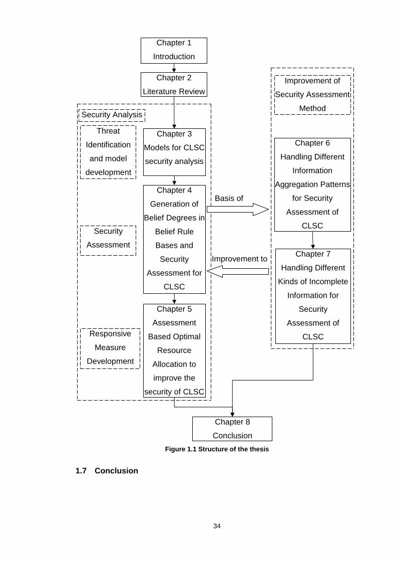
In summary, among the 8 chapters, Chapter 1 and Chapter 8 are the
background and the conclusion of the research, while Chapter 2 is the review
33
on the current research related to risk and security analysis under the context of
CLSC. The aim of Chapter 3 and Chapter 4 is to propose an analytical model to
assess CLSC security. Specifically, in Chapter 3, after threats faced by CLSC
and factors which may influence CLSC security are identified, a general model
to assess security level of general CLSC and a specific model to assess
security level of a port storage area along a CLSC against cargo theft are
developed. In Chapter 4, belief degrees in BRBs for the specific security
assessment model developed in Chapter 3 are generated by a novel process,
based on which the security assessment results for 5 different ports against
cargo theft are given by the direct application of RIMER. According to the
assessment results generated by RIMER in Chapter 4, in Chapter 5, optimal
resource allocation strategies are developed for security improvement of CLSC
under the constraints of available resources, which can be considered as the
development of responsive measures after the security level is assessed.
Following the identification of the limitations of RIMER in handling security
assessment problem in Chapter 4, Chapter 6 and Chapter 7 can be considered
as the improvement of the capability of RIMER for security assessment under
the context of CLSC, focusing on accommodating and handling different
information aggregation patterns and different kinds of incompleteness,
respectively. The above discussion shows that the threats faced by CLSC and
the factors influencing CLSC security are identified in Chapter 3, security
assessment is conducted in Chapter 4 based on the generated BRBs, and in
Chapter 5 responsive measures according to the assessment result are
developed. Therefore, Chapter 3 to Chapter 5 can be considered as a process
of security analysis, including threat identification, security assessment and
responsive measures development. To improve the rationality of security
analysis, Chapter 6 and Chapter 7 are proposed to improve the capability of the
assessment method applied in Chapter 4.
The relations of different chapters of the thesis can be represented in Figure 1.1
as follows:
34
Figure 1.1 Structure of the thesis
1.7 Conclusion
Improvement to
Basis of
Chapter 1
Introduction
Chapter 2
Literature Review
Chapter 3
Models for CLSC
security analysis
Chapter 4
Generation of
Belief Degrees in
Belief Rule
Bases and
Security
Assessment for
CLSC
Chapter 5
Assessment
Based Optimal
Resource
Allocation to
improve the
security of CLSC
Chapter 6
Handling Different
Information
Aggregation Patterns
for Security
Assessment of
CLSC
Chapter 7
Handling Different
Kinds of Incomplete
Information for
Security
Assessment of
CLSC
Chapter 8
Conclusion
Security Analysis
Threat
Identification
and model
development
Security
Assessment
Responsive
Measure
Development
Improvement of
Security Assessment
Method

35
The aim of this chapter is to provide an overview of the research conducted in
the thesis, including research background, questions, aims and objectives,
methodologies, originalities and beneficiaries. In addition, the content of each
chapter in the thesis and the logic relationship among them are also introduced
and analyzed in detail.
36
2 Chapter 2 Literature Review
Abstract
In this chapter, current literature relevant to the research conducted in the thesis
is reviewed, including the research on CLSC security, the research on risk
analysis methods with their applications in the areas relevant to CLSC security
assessment, the research on resource allocation in response to security and
safety incidents and the research on current methods to aggregate information
for Multiple Criteria Decision Analysis problems. Moreover, the limitations of
current research are analyzed, and the selection of RIMER as a basic tool for
CLSC security analysis is justified accordingly.
2.1 Introduction
As revealed by the discussion in Chapter 1, CLSC plays a dominant role in
world cargo transportation due to its high efficiency, and at the same time, it
also faces various threats due to its vulnerability. Therefore, ensuring security of
CLSC is “the most important challenge” faced by CLSC executives (Sarathy,
2006). Correspondently, there is more and more research on security issues of
CLSC in recent years, especially after the 9-11 terrorist attack. In this chapter,
such research is reviewed first. In addition, since security assessment is one of
the core tasks in security analysis, current risk analysis and risk assessment
methods with their applications in the areas relevant to CLSC security
assessment are reviewed subsequently. Apart from security assessment, how
to optimally allocate limited resources to improve CLSC security based on
security assessment result is another important task in CLSC security analysis,
thus, a review on the research on resource allocation in response to security
and safety incidents is also provided. Furthermore, for CLSC security
assessment, the essence of the assessment process is to aggregate
information in the assessment model, it is necessary to investigate the
rationality of such information aggregation, correspondently, the research on
current methods for information aggregation for MCDA problems is reviewed.
Based on the literature reviewed, the limitations of current research for CLSC
security analysis and the requirements on CLSC security analysis are proposed,

37
accordingly, RIMER is selected as the basis for CLSC security analysis in this
thesis due to its advantages compared with other methods reviewed in this
chapter.
2.2 Research on CLSC security
2.2.1 Basic definitions
Prior to reviewing current research on security issues in CLSC, some concepts
need to be defined to clarify the boundary of the research conducted in the
thesis and to provide a basis for all the discussions in the thesis.
Specifically, as the thesis mainly focuses on CLSC security analysis, the
concepts of security should be defined. In addition, for some other terms which
are closely related to security, such as risk, threat, hazard and especially safety,
their concepts should also be defined for the clarification of the scope of
security.
Currently, for different purposes, there are different definitions of risk, safety,
security, hazard, threat and other related terms from different points of view
(Firesmith, 2003; Jonsson, 1998; Lau, 1998; Sørby, 2003; Willis and Ortiz,
2004). According to the content of the research in this thesis and the opinions of
different PFSOs from interviews, the definitions which are used in this thesis are
based on those proposed in (Firesmith, 2003):
• Safety: the degree to which accidental harm is prevented, detected, and
reacted to;
• Security: the degree to which malicious harm is prevented, detected, and
reacted to;
• Hazard: a situation that increases the likelihood of formation of one or
more related accidental harms;
• Threat: a situation that increases the likelihood of formation of one or
more related malicious harms;
• Risk: a term which is used to describe the likelihood of occurrence and
the consequences of a hazard or a threat. Accordingly, risk can be

38
categorized as hazard based risk and threat based risk. The ‘risk’
discussed in this paper mainly refers to threat based risk.
From the above definitions, we can see that threat, threat based risk and
security are the terms regarding malicious harm, while hazard, hazard based
risk and safety are the terms regarding accidental harm. In addition, the relation
among threat, threat based risk and security can be analyzed as follows: threat
represents a certain state of a situation; threat based risk considers both
likelihood of the threat and potential consequence caused by the threat; in
addition to the likelihood and the potential consequence, security also considers
the features of the party which is under the threat. Similar conclusion can be
drawn for the relation among hazard, hazard based risk and safety.
2.2.2 Research on security issues in CLSC from a ge neral level
One of the most typical documents in this category is the ISPS Code (IMO,
2002a), which was issued by IMO in 2002. This code is released in response to
the “perceived threats to ships and port facilities in the wake of the 9/11 attacks
in the United States” (PECC, 2004). It is a “comprehensive set of measures to
enhance the security of ships and port facilities” (IMO, 2002a), which covers the
specifications of general responsibilities of contracting governments and ship
companies; the general responsibilities of security officers in ship companies,
individual ships and ports; the descriptions of different security levels of both
ships and port facilities; the general requirements on development; the training
and drilling of ship and port facility security plans; the verification and
certification for ships, and so on.
As nearly all CLSCs are operating internationally, customs, with their unique
authorities and expertise, play a central role in ensuring CLSC’s security (WCO,
2007). Correspondently, in 2007, WCO issued a SAFE Framework of Standards
(WCO, 2007) to secure and also facilitate the movement of global trade. This
framework is mainly based on two aspects: Customs-to-Customs network
arrangements and Customs-to-Business partnerships. The former has 11
standards while the latter has 6 standards. In the standards, the responsibilities
of different organizations along a whole chain of cargo custody, from stuffing
39
site to unloading site, which were always ambiguous in the past, are clearly
stated.
Another set of important documents relevant to CLSC security is the ISO 28000
series (ISO, 2007a; ISO, 2007b; ISO, 2007c; ISO, 2007d), which are the
standards on security management systems for supply chains (LRQA, 2009;
Piersall, 2007). Among the series, ISO 28000 (ISO, 2007a) is a general
specification which introduces the elements for security management systems,
including security management policy, security risk assessment and planning,
implementation and operation for security management, checking and
corrective actions, management review and continual improvement. ISO 28004
(ISO, 2007d) is a detailed explanation on ISO 28000, which explains each part
of ISO 28000 in 4 dimensions, i.e., intent, typical inputs, process and typical
output of each part.
Besides the documents issued by international organizations, some regional
initiatives are also developed. For example, in Europe, the ISPS Code is
incorporated into the EC Regulation 725/2004 (EC, 2004; TRANSEC, 2011);
EC Regulation 884/2005 sets the procedures for conducting EC inspections in
the field of maritime security (EC, 2005a); and EC Directive 65/2005 aims at
enhancing security throughout ports (EC, 2005b; TRANSEC, 2011). In addition,
Authorised Economic Operator (AEO) is introduced by EC to CLSC operators in
Europe in 2005 (EC, 2005b) to encourage organizations involved in CLSCs to
enhance security in their operation.
All the documents mentioned above focus on sea transportation of cargo.
However, in CLSC, a container’s voyage contains not only sea transportation
but also inland transportation, the security issues of which need to be
considered as well. As such, the International Shippers and Freight Forwarders
Security Code (ISFFS Code) was proposed in 2003 by International Trade
Procedures Working Group (ITPWG) of United Nations Centre for Trade
Facilitation and Electronic Business (UN/CEFACT) (ITPWG, 2003). This code
mainly develops a set of requirements to ensure the security of cargo
transported by road, rail or inland waterways, including requirements on stuffers
40
and packers; requirements on warehouses, storage areas and terminals;
requirements on forwarders and transporters; requirements on information
processors, and so on. For each category, the requirements are further
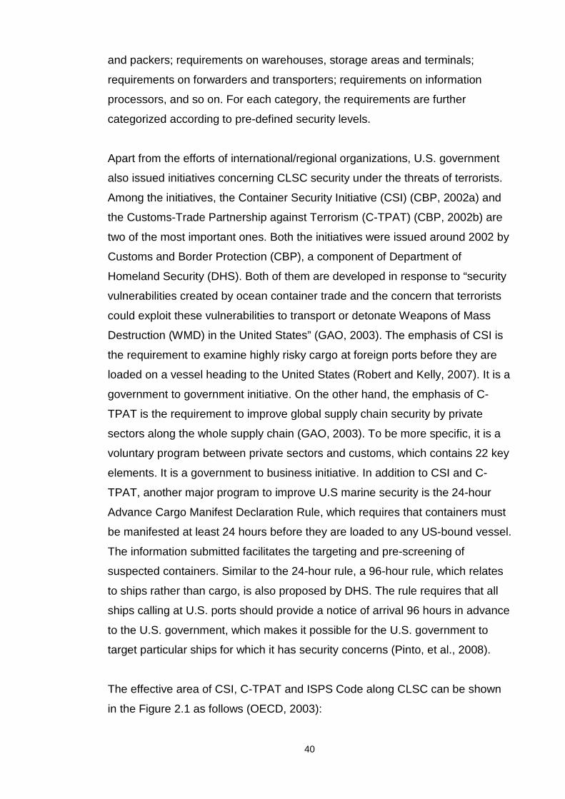
categorized according to pre-defined security levels.
Apart from the efforts of international/regional organizations, U.S. government
also issued initiatives concerning CLSC security under the threats of terrorists.
Among the initiatives, the Container Security Initiative (CSI) (CBP, 2002a) and
the Customs-Trade Partnership against Terrorism (C-TPAT) (CBP, 2002b) are
two of the most important ones. Both the initiatives were issued around 2002 by
Customs and Border Protection (CBP), a component of Department of
Homeland Security (DHS). Both of them are developed in response to “security
vulnerabilities created by ocean container trade and the concern that terrorists
could exploit these vulnerabilities to transport or detonate Weapons of Mass
Destruction (WMD) in the United States” (GAO, 2003). The emphasis of CSI is
the requirement to examine highly risky cargo at foreign ports before they are
loaded on a vessel heading to the United States (Robert and Kelly, 2007). It is a
government to government initiative. On the other hand, the emphasis of C-
TPAT is the requirement to improve global supply chain security by private
sectors along the whole supply chain (GAO, 2003). To be more specific, it is a
voluntary program between private sectors and customs, which contains 22 key
elements. It is a government to business initiative. In addition to CSI and C-
TPAT, another major program to improve U.S marine security is the 24-hour
Advance Cargo Manifest Declaration Rule, which requires that containers must
be manifested at least 24 hours before they are loaded to any US-bound vessel.
The information submitted facilitates the targeting and pre-screening of
suspected containers. Similar to the 24-hour rule, a 96-hour rule, which relates
to ships rather than cargo, is also proposed by DHS. The rule requires that all
ships calling at U.S. ports should provide a notice of arrival 96 hours in advance
to the U.S. government, which makes it possible for the U.S. government to
target particular ships for which it has security concerns (Pinto, et al., 2008).
The effective area of CSI, C-TPAT and ISPS Code along CLSC can be shown
in the Figure 2.1 as follows (OECD, 2003):
41
Figure 2.1 Effective area of CSI, C-TPAT and ISPS C ode
More recently, DHS issued a “Strategy to Enhance International Supply Chain
Security” (DHS, 2007) in response to the Security and Accountability For Every
Port Act (SAFE Port Act) (US Congress, 2006), which is a public law aiming to
improve maritime and cargo security through enhanced layered defences. The
strategy issued by DHS intends to establish an overarching framework for the
secure flow of cargo through supply chains. The strategy identifies critical nodes
along an international supply chain, delineates the roles and responsibilities of
different organizations involved, and most importantly explains necessary
responsive activities and factors that need to be considered during the recovery
process after a disruption. These response and recovery issues are seldom
mentioned in other similar documents.
In addition to the documents issued by governmental and international/regional
organizations, some industrial organizations also developed certain initiatives
for CLSC security. For example, TAPA developed a set of requirements and
standards to assess the security of organizations involved in CLSC, such as
Freight Security Requirement (FSR) which specifies the minimum acceptable
standards for security throughout the supply chain and the methods to be used
in maintaining those standards (TAPA, 2011), and Trucking Security
Requirement (TSR) which specifies the minimum acceptable standards for
security throughout the supply chain utilizing trucking and associated operations
and the methods to be used in maintaining those standards (TAPA, 2008). TSR
may be used in conjunction with FSR.
42
Further, some academic papers also discuss security related issues in CLSC
from a general level. For example, current legislations on port safety and
security are reviewed and current security situations faced by ports and EU
inter-model transportation are discussed (Psaraftis, 2005). Security measures
taken by the U.S. government and international organizations are reviewed and
the development of a global agreement to ensure security of CLSC is also
suggested to link security and other maritime trade-related issues together
(Stasinopoulos, 2003). Key shore-based and near shore activities associated
with maritime operations, which are currently not covered by ISPS Code, are
identified, relationships among the activities are investigated, and key criteria for
a good marine security management system are studied (Paulsson, 2003). The
impacts of CSI on maritime supply chains, especially financial impacts are
analyzed in general by Banomyong (2005). In addition, Helmick discusses what
had been done and what should be done in the field of port and marine security
(Helmick, 2008), indicating that further refinement and standardization of risk
based decision methodologies and applications are clearly needed, including
comprehensive threat assessment, the consideration of vulnerability variables
through the whole global supply chain, the quantification of relative risks and
uniform risk assessment methodologies, etc.
In a word, this stream of research focuses on a general level, aiming at
developing and discussing strategies, policies, principles, specifications,
requirements, etc. to enhance CLSC security. It is the basis and general
guidelines of all the research on security issues in CLSC. However, this stream
of research is too general for the development of analytical CLSC security
analysis models.
2.2.3 Research on specific issues of security in CL SC
2.2.3.1 Research on features of CLSC and threats faced by CLSC Considering the features of CLSC and threats faced by CLSC, OECD issued
several reports. In the report issued in 2005 (OECD, 2005), which concentrates
on container transport security across inland and marine transport mode under
the potential threat of containers being used by terrorists as a delivery vehicle
for chemical, biological, radiological or nuclear (CBRN) weapons, the features

43
of a container transport chain are analyzed in detail. Based on the analysis, the
nature of CBRN threat is also revealed. In the report issued in 2003 (OECD,
2003), threats faced by maritime transport are analyzed based on the following
categories: cargo, vessels, people, finance/logistics support and trade
disruption. Research in the above areas can provide general knowledge on how
CLSC is operating and how vulnerable CLSC is to different threats. The
knowledge provides a background for CLSC security analysis.
2.2.3.2 Research on security assessment criteria of CLSC and components of security plans in CLSC
In some literature, general criteria for CLSC security assessment are analyzed
and the essential components of security plans are discussed.
In ISPS Code (IMO, 2002a), the topics of security assessment and security
plans for both ships and port facilities are two of the most important contents. In
the Code, data required by security assessment and components required to
develop a security plan are specified in detail.
In the SAFE Framework of Standards (WCO, 2007), elements considered by
AEO and customs can be broadly divided into several categories, including
cargo security, conveyance security, premises security, personnel security,
trading partner security and crisis management & incident recovery. These
categories indicate high-level criteria when CLSC security needs to be
assessed.
In ISO 28001 (ISO, 2007b), the best practices for implementing supply chain
security assessments and security plans are discussed, including process and
criteria for security assessment and essential components for a security plan in
a general level.
Another literature about assessment criteria is a report issued by RAND
Cooperation in 2004, which is one of the first of a series of studies on the topic
of supply chain security (Willis and Ortiz, 2004). In the report, five capabilities,
regarding the efficiency and security of global container supply chain, are

44
proposed, and the capabilities can be considered as general criteria for CLSC
security assessment.
The criteria discussed in the above literature are proposed according to different
emphases on security issues in CLSC from different points of view. A
comprehensive understanding of the criteria can help to construct a set of high-
level attributes for CLSC security assessment. Research on essential
components of a security plan reveals essential aspects to be considered to
respond to different security incidents, which is also important for security
assessment since responding capability is one of the elements which needs to
be considered when CLSC security is assessed and analyzed.
2.2.3.3 Research on countermeasures of CLSC facing different threats The countermeasures of CLSC against different threats can be roughly divided
into 3 categories: managerial measures, operative measures and technical
measures.
Managerial countermeasures refer to policies, regulations, requirements or
general methodologies used to respond to threats faced by CLSC. For example:
in ISO 28001 (ISO, 2007b), a general methodology for developing
countermeasures is proposed; in ISO 28003 (ISO, 2007c), regulations for audit
or certification agencies of supply chain security management systems are
discussed; in the WCO Safe Framework of Standards (WCO, 2007),
requirements on the information of imported and exported cargo are provided,
which needs to be submitted to customs; regulations about how to provide
critical data of maritime security incidents to first responders are developed
(Wydajewski and White, 2002).
Operative countermeasures refer to actions taken by different operators in
CLSC to make it more secure. In C-TPAT (CBP, 2002b), 22 key elements are
proposed. The operative countermeasures mentioned in the elements include
employee background checks, inspection of empty containers, and so on. The
operative countermeasures proposed by Bakir (2007) include access control,
security awareness training, standardization of paperwork security and

45
maintaining the security of warehouse perimeters. Other operative
countermeasures include continuously reviewing and updating security
procedures (Closs and McGarrell, 2004), developing contingency plans (Tang,
2006), securing container integrity (OECD, 2005), and so on.
Technical countermeasures refer to technologies which can be used to enhance
CLSC security. The countermeasures include the application of newly
developed information technologies (Noda, 2004) and data mining technologies
(Lee and Wolfe, 2003), the implementation of Non-Intrusive Inspection (NII)
technologies like X-ray or Gamma-ray scanning (Hessami, 2004), the
introduction of so-called ‘smart containers’ (Kim, et al., 2008; Robert and Kelly,
2007), Radio Frequency Identification (RFID) technique (Yoon. et al, 2007),
tracking technique (David, 2005 ; Tsamboulas, 2010), high capable seals
(McCormack, et al., 2010; Tirschwell, 2005 ; Tsamboulas, 2010) and so on.
Note that the above 3 categories of countermeasures are not independent of
each other, e.g., managerial countermeasures are implemented through
operative countermeasures, while technical countermeasures provide support
to both managerial countermeasures and operative countermeasures.
All the 3 categories of countermeasures mentioned above can provide ideas on
how to improve CLSC security and which factors should be considered when
CLSC security is assessed and analyzed.
2.2.3.4 Research on cost and performance estimation for implementation of security related measures
The report issued by OECD in 2003 (OECD, 2003) proposes a method to
estimate costs for implementation of different initiatives to enhance maritime
security. Specifically, it mainly estimates the implementation costs of ISPS
Code through the estimation of costs to implement each part of the Code.
Performance estimation can be found from a series of reports issued by United
States Government Accountability Office (GAO). One of the roles of GAO is to
assess the performance of CSI and C-TPAT during their implementation. Based
on the assessment, recommendations can be generated to help CBP improve
46
the performance of CSI and C-TPAT. In 2003, shortly after CSI and C-TPAT
were implemented, GAO issued the first report to assess their performance
(GAO, 2003). One of the problems revealed by GAO in the report is that there
lacks a set of criteria to measure the performance and achievements of the two
initiatives. In 2005, another report (GAO, 2005a) was issued by GAO to follow
up the recommendations proposed in the previous report. In this latter report, it
was stated that progress had been made in developing performance criteria for
assessing the initiatives’ performance, but the criteria mainly focused on the
performance of information sharing and collaboration among CSI and host
country personnel, and they could not be used to measure the effectiveness of
CSI targeting and inspection activities. Following this assessment result, CBP
refined overall CSI performance criteria, but the criteria for core CSI functions
are still absent, as indicated in a report issued by GAO in 2008 (GAO, 2008).
In CLSC security analysis, one of the most important tasks is to allocate
resources, e.g., budgets, human resources, hardware facilities, etc. to improve
the security of organizations involved in CLSC. As resources are always limited,
it is necessary to utilize resources in an efficient and effective way. Accordingly,
the consumption of resources for different alternatives to improve security
should be estimated. As budgets are the most common resources for security
improvement, the estimation of costs incurred by implementing different security
improvement alternatives is very important. In addition, different measures for
security improvement have different impact on security, so performance
estimation is also essential for security analysis as the impact of different
measures on the performance of relevant factors related to CLSC security
should be estimated. The literature reviewed in this part can provide a rough
and initial idea on how cost and performance can be estimated.
2.2.3.5 Summary The research reviewed in this section aims at exploring different aspects of
CLSC and is more specific than what is discussed in Section 2.4. Several
preliminary ideas, which can be applied and further developed in the research
on security analysis in CLSC, are discussed in this section. However, nearly all
these ideas are proposed in a subjective and descriptive way and there lacks an
47
analytical and structured model for CLSC security analysis, which can help to
generate practical and specific suggestions on how CLSC security can be
maintained.
2.3 Research on risk analysis methods with their ap plication in the areas relevant to CLSC security assessment
When risk and security assessment methods are discussed, the most
fundamental question is how to model the concept of risk and security. In other
words, what are the basic components of risk and security? Usually, risk is
described by two components, i.e., the likelihood of occurrence of an
undesirable event and the severity of its consequences (Aagedal et al., 2002;
Bahr, 1997; Butler, 2002; IMO, 2002b; Li and Cullinane, 2003). Although
security shares some common characteristics with risk, there are still subtle
differences between these two concepts, as discussed in Section 2.2., and thus
components used to analyze and model risk and security may not be exactly
the same. However, components appropriate for security modelling are not
widely discussed in previous research.
Based on the components of risk, different methods for risk analysis are
proposed, but few of them are specifically applied to risk assessment under the
context of CLSC. Thus, the methods reviewed in the following are mainly about
risk analysis in general supply chains or risk assessment in individual marine
operations.
The research on risk analysis in general supply chains began only recently
(Khan and Burnes, 2007; Rao and Goldsby, 2009), and most research is
conducted in a descriptive and qualitative way. For instance, the relation
between product design and supply chain risk was discussed (Khan et al.,
2008); a conceptual framework for supply chain risk management was
developed (Manuj and Mentzer, 2008); a general framework for natural disaster
response of a supply chain was proposed based on interviews with logistics
managers (Perry, 2007); while Christopher and Lee (2004) discussed the
impact of visibility on supply chain risk; and Giaglis et al. (2004) proposd an
architecture for minimization of logistics risk by routing vehicles in real time

48
using mobile technologies. On the other hand, for limited quantitative research
related to risk issues in general supply chains, some discussions lie in the
analysis of inventory risk, demand risk, supply risk and transportation risk for
individual organizations in supply chains (Tomlin, 2006; Towill, 2005; Wilson,
2007), while other discussions focus on modelling relationships among supply
chain risk and supply chain efficiency and profitability (Agarwal and Seshadri,
2000; Wang and Webster, 2007). In summary, for risk analysis in general
supply chains, there is not enough analytical research conducted, and among
the limited research conducted quantitatively, information needed for risk
analysis models is measured numerically. In addition, in existing quantitative
research, very limited attention has been paid to the analytical risk assessment
of the whole supply chain.
Among the methods for risk analysis related to marine operations, Formal
Safety Assessment (FSA) is widely applied, which is introduced by IMO as “a
rational and systematic process for assessing the risks associated with shipping
activity and for evaluating the costs and benefits of IMO's options for reducing
these risks” (IMO, 2002b). According to FSA, safety assessment is conducted
through the following 5 steps: hazard identification, risk analysis, Risk Control
Options (RCO) development, Cost Benefit Assessment (CBA) and
recommendations for decision making. In addition to the introduction by IMO,
there are also some academic papers discussing the topic of FSA. For example,
FSA is applied to analyze risk in individual containerships (Wang and Foinikis,
2001), cruise ships (Lois, et al., 2004) and general ships (Wang, 2001); it is also
introduced with several practical applications in the UK, Germany and some
Scandinavian countries (Soares and Teixeira, 2001); in addition, a review
process, i.e., FSA qualification, is introduced to support the consolidation of
confidence in FSA results (Rosqvist and Tuominen, 2004) and a critical review
of FSA with detailed introduction and analysis for each step of FSA is also
proposed (Kontovas and Psaraftis, 2009). Although FSA has been adopted by
IMO since 2002, and it has been applied in various situations by researchers, it
also has its limitations. For example, FSA only provides a general framework
and process for safety analysis, and there is limited practical guidance on how
to conduct different steps in the process; when FSA is applied in different

49
situations, risk is usually represented by an index number (Kontovas and
Psaraftis, 2009; Lois, et al., 2004; Rosqvist and Tuominen, 2004; Wang and
Foinikis, 2001), which may lead to information loss (Kontovas and Psaraftis,
2009); in addition, the uncertainty, which is prevalent in risk and safety analysis
in maritime operation, are seldom discussed in the applications of FSA; further,
all the applications of FSA focuses on individual maritime operators instead of a
whole supply chain.
Another category of methods for risk analysis related to marine operation is
based on probabilities. For example, Event Tree Analysis (ETA) are applied for
vulnerability assessment of a maritime transportation system (Ø. Berleetal et al.,
2011); both Fault Tree Analysis (FTA) and ETA are introduced to risk
assessment in shipping and ports (Bichou, 2008); in addition, Fault Trees and
Event Trees are used to model a general risk management framework for a
maritime supply chain (Yang, 2011), and ETA and FTA are also introduced
under the framework of FSA (Kontovas and Psaraftis, 2009). In addition to FTA
and ETA, Bayesian Network (BN) is another tool used for risk analysis in the
areas relevant to CLSC. Specifically, BN is used under the framework of FSA
by Kontovas and Psaraftis (2009), it is also used to assess safeguards to
secure supply chains (Pai, et al., 2003) and to assess risk of container supply
chain (Yang, 2006). Although ETA, FTA and BN have the capability to handle
uncertainty involved in security analysis in CLSC, they can only handle the
uncertainty caused by randomness. However, due to the complexity of CLSC
operation, not all uncertainty involved in CLSC security analysis are caused by
randomness, and uncertainty can also be caused by fuzzy information or
ignorance in subjective judgments. In addition, the precise probabilities required
by ETA, FTA and BN are usually very difficult to generate under the context of
CLSC security analysis, as there is usually insufficient historic data available to
generate probabilities in an objective way (Bichou, 2008). Even available
information is usually not sufficient for experts to specify probabilities according
to their subjective knowledge.
To avoid specification of precise probabilities, Fuzzy Logic is applied for risk
analysis in port operations (Ung, 2007), offshore engineering (Ren, et al., 2009)
50
and container supply chains (Yang, 2006). However, the rationality of fuzzy
arithmetic is always arguable, and the way to aggregate information based on
fuzzy logic leads to information loss.
Moreover, some methods in Artificial Intelligence are applied for risk analysis for
marine operations and one of the examples is the application of Artificial Neural
Network (ANN) to risk assessment in port operations (Ung, 2007). Although
ANN is a well developed method, it is a ‘black box’ method which cannot
explicitly show its inference process.
Apart from the above methods, the Evidential Reasoning (ER) approach, which
is based on Dempster-Shafer theory (Shafer, 1976), was developed in early
1990’s (Yang and Singh, 1994) and improved in 2000’s (Yang and Xu, 2002).
The ER approach has been applied to analyze risks in offshore engineering
systems (Liu, et al. 2005; Ren, et al., 2005; Sii, et al., 2005) and to assess risk
of container supply chains (Yang, 2006). Compared with the methods reviewed
above, the ER approach has the following two major advantages: 1) it has a
solid mathematical basis (Shafer, 1976); and 2) with the introduction of the
concept of belief distribution, information with different features and different
kinds of uncertainty can be accommodated and handled by the ER approach
under a unified framework, and there is no information loss during the reasoning
process. Based on the ER approach, RIMER was proposed (Yang, et al., 2006).
Under the framework of RIMER, belief distributions are used to model both
individual factors threatening CLSC security, and BRBs, which incorporates
belief distributions into conventional rule bases, are applied to model the
relations among the factors. Apart from the advantages of the ER approach as
mentioned above, RIMER is capable and flexible in representing knowledge
contained in inference models, and unlike ANN which is a ‘black box’ method,
the inference process of RIMER is transparent.
From the above discussion, it can be seen that compared with other methods
as reviewed above, it is more appropriate to use RIMER as a basic tool for
CLSC security assessment.

51
2.4 Research on resource allocation in response to security and safety incidents
In CLSC security analysis, in addition to security assessment, it is also
important to know how to improve security level of CLSC based on the security
assessment result. As the resources for CLSC security improvement are always
limited, it is essential to investigate how to allocate the resources so that they
can be applied in an efficient and effective way.
Generally, the current research on resource allocation to respond to security
and safety incidents can be roughly divided into the following 2 categories:
• Allocating resources to respond to emergent incidents which need
immediate response, such as earthquake, hurricane, forest fire, and
other general disasters. For example, Fiedrich et al. (2000) developed a
dynamic programming model to generate an optimal strategy to minimize
fatalities under the constraint of available resources after an earthquake;
Minciardi et al. (2009) developed a mathematical programming model to
provide an optimal solution to allocate resources to minimize unsatisfied
demand, inappropriate resource assignment and relevant cost for an
emergency due to natural hazard events; in addition, a mathematical
programming model was proposed with the objective to minimize both
estimated damage and transfer cost after a forest fire (Fiorucci, 2004);
and a Decision Support System (DSS) is introduced for resource
allocation in disaster management, and the central part of the DSS is a
mathematical programming model to minimize the cost of dispatching
resources (Kondaveti, 2009).
• Risk Based Resource Allocation: this stream of research only begins
recently and it is mainly conducted for grant allocation in DHS among
different states within the US. Currently, the grants are allocated based
on a 40/60 scheme and the criteria to allocate the budget in the scheme
is the population size of different states (Brunet, 2005; Quadrifoglio, 2008)
without the consideration of actual risk faced by the states. Regarding
the 40/60 scheme, critiques are proposed by researchers (De Ruby,

52
2005; Quadrifoglio, 2008; Reifel, 2006) and it is recommended that
“homeland security assistance should be based strictly on an
assessment of risks and vulnerabilities” (9/11 Commission, 2004). In
addition, considering the security of maritime, according to a report
issued by GAO, both federal law and Homeland Security Presidential
Directive 7 (HSPD-7) suggest resources be allocated in a risk based way
to ensure port security (GAO, 2005b), furthermore, it is suggested that
“maritime security, specifically port security, is one area where DHS has
attempted to implement risk-based resource allocation” (Reifel, 2006).
Regarding the specific method to assist risk based resource allocation,
Reifel (2006) proposes a mathematical programming model to maximize
risk reduction subject to funding constraints while Quadrifoglio (2008)
proposes a model to minimize both cost and risk under the limit of
available budget.
However, under the context of resource allocation regarding security issues in
CLSC, both categories of research mentioned above have limitations:
• For the first category of research regarding resource allocation in
emergency response, the actual security or risk level of the situation to
which the resources are allocated is not explicitly considered. Without the
consideration, all the areas under the impact of the emergent incident
have the same priority to get the limited resources, despite the fact that
some areas may need the resources more urgently because they are
under a lower security level. Further, in CLSC, there are so many areas
to consider when security needs to be improved that it is impractical for
security officers to allocate the limited resources to all the areas.
Therefore, an assessment is needed before allocating resources, and the
areas with a security level which is above a satisfactory threshold will not
be taken into consideration when resources are allocated. In this way,
the limited resource to improve security within CLSC can be allocated
more efficiently and effectively.
• To allocate limited resources based on security level is similar to risk
based resource allocation proposed by researchers in DHS as reviewed
53
above. However, as risk based resource allocation approach is still in its
infancy (Quadrifoglio, 2008), there is no detailed guidance on how to
conduct such approach, especially under a complex situation where
uncertainty is prevalent.
• For specific methods to allocate resources in both categories of research,
they are applied based on the assumption that the resource allocation
problem can be modelled in a precise and deterministic way. Specifically,
it is assumed that all the variables can be represented by numerical
values and the relation among the variables can be modelled by precise
mathematical formula without uncertainty involved. However, under the
context of CLSC security analysis, due to the complexity of CLSC
operation, it is likely that not all the variables in the resource allocation
problem can be represented by numerical values and it is difficult to
always model the relation among the variables of the problem in a
precise manner. In addition, different kinds of uncertainty are also
prevalent in measuring the variables and in modelling the relations
among them. Therefore, to model an optimal resource allocation problem
under CLSC, a semi-structured framework with the capability to
accommodate and handle different forms of information with different
kinds of uncertainty is more suitable than a set of numerical variables
with a set of precise mathematical formula to represent the relations
among the variables.
On the other hand, as discussed previously, belief distributions can be used to
model different forms of information and different kinds of uncertainty regarding
the various factors threatening security of CLSC, and by incorporating belief
distributions, BRB is a semi-structured model which can provide a flexible
scheme to accommodate and handle different forms of information with different
kinds of uncertainty existing in the relation among the factors. In addition, based
on BRBs, RIMER can be applied to assess CLSC security level. Therefore, in
this thesis, based on the security assessment results generated using RIMER,
the security related factors with security level below a satisfactory threshold are
identified and limited resources are allocated to improve the security of the
identified factors in an efficient and effective way.
54
2.5 Research on existing methods for information ag gregation for Multi Criteria Decision Analysis problems
When RIMER is applied for CLSC security assessment, the essence of the
assessment process is to aggregate information of the factors in the lower level
in the security assessment model to form the information of the factors in the
corresponding higher level in the security assessment model. Accordingly, the
CLSC security assessment problem can be considered as an MCDA problem,
in which, the information of each factor in the lower level can be considered as
the measurement of individual criterion in a MCDA problem while the
aggregated information of the factor at the corresponding higher level can be
considered as the assessment of an alternative in the MCDA problem.
Due to the complexity of CLSC, the relations among different factors in the
CLSC security assessment model are various, which makes it necessary to
develop and handle different patterns for information aggregation in CLSC
security assessment problem. In this section, current methods for information
aggregation under the context of MCDA are reviewed. Based on the features of
the methods reviewed, the selection of RIMER as a framework to handle
different information aggregation patterns is justified.
One broad category of methods to aggregate information in MCDA problems is
the so called “out ranking” methods, ELECTRE (Roy, 1968) and PROMETHEE
(Brans et al., 1984) are two typical examples in such a category. In the “out
ranking” methods, alternatives are usually compared two by two to generate the
degree of preference of one alternative over the other with respect to a criterion.
After all these preference relations are generated, they are then aggregated to
take all the criteria into account to generate partial ordering of the alternatives
(Garish, 1995). The most obvious limitation of such methods is that the
performance of each alternative itself cannot be generated. If such methods are
used to assess security of several CLSCs, the ranking of the security level of
different CLSCs can be generated while it is not clear how secure each CLSC is.
55
Another category of information aggregation methods aims at generating the
overall performance of each alternative for comparison instead of the “ranking
relation” among the alternatives.
In this category, the simplest method for information aggregation is Min/Max
function (Beliakov et al., 2007; Xu and Da, 2003), which takes
minimum/maximum value of the factors to be aggregated as the aggregation
result. Similar to Min and Max, AND and OR are also considered as operators
to aggregate information. To use Min, Max, AND or OR for information
aggregation, the essential assumptions are: 1) the information of each factor to
be aggregated can be measured in a numerical or binary way, and 2) there is
no compensation among the factors to be aggregated. However, such
assumptions are not realistic in many MCDA problems due to the following facts:
1) the factors to be aggregated may have different natures due to the
complexity of a problem, thus it is not practical, if not impossible, to always
represent their information in a quantitative way (Chang and Chen, 1994;
Dubois et al., 1998; Dulmin and Mininno, 2003; Herrera et al., 2005; Yeh and
Chang, 2009). 2) In an MCDA problem, there are usually some degrees of
compensation among the factors to be aggregated (Dulmin and Mininno, 2003).
Until now, the most common and widely applied method for information
aggregation is weighted arithmetic mean (Edwards, 1977; Garish and
Labreuche, 2007; Grabisch, 1996; Marichal, 1998; Marichal, 2000a; Marichal,
2002; Tzeng et al., 2005) and Ordered Weighted Average (OWA) with its
generalizations (Godo and Torra, 2000; Xu, 2007; Xu and Da, 2003; Yager,
1988). This category of aggregation patterns, especially weighted arithmetic
mean, has its advantages, such as it is easily to be understood and
conveniently to be applied, however, its limitations are also obvious, as
discussed in many literatures (Edwards, 1977; Godo and Torra, 2000; Grabisch,
1996; Luo and Jennings, 2007; Marichal, 1998; Marichal, 2000a; Marichal,
2000b, Marichal, 2002; Tzeng et al., 2005). Besides the requirements that the
information of the factors to be aggregated need to be represented in a
quantitative way, the other limitations of arithmetic mean and OWA include the
requirements that 1) the factors with information to be aggregated should be
56
independent of each other, 2) the factors with information to be aggregated can
be fully compensated among each other, i.e., poor performance of a certain
factor can be always fully compensated by good performance of other factors, 3)
the factors with information to be aggregated should have the same nature. On
the other hand, in many situations, the factors to be aggregated are not
independent with each other due to the interaction among them (Marichal,
2000a; Marichal, 2000b; Tan and Chen, 2010; Tzeng et al., 2005), and full
compensation is also not always rational among the factors (Dulmin and
Mininno, 2003), further, the factors to be aggregated in the CLSC security
assessment model may have completely different natures due to the complexity
of CLSC.
Facing the critiques on using weighted arithmetic mean to aggregate
information, fuzzy measures are introduced as a framework to accommodate
different forms of information of parent factors with different natures, and then
such fuzzy measures are aggregated to generate the overall performance of the
child factor (Chang and Chen, 1994; Cheng, 1999; Herrera et al., 2005;
Martinez et al., 2007; Yeh and Chang, 2009). Two of the most widely used
aggregation operators in fuzzy set theory are T-Norm and T-Conorm
(Detyniecki, 2001; Dombi, 1982; Fung and Fu., 1975; Klement et al., 2000),
however, their main limitation in terms of aggregation is that the result is not a
compromise between low and high ratings (Luo and Jennings, 2007), i.e., the
factors with information to be aggregated cannot be compensated by each other.
In addition to T-Norm and T-Conorm, various fuzzy arithmetic operators are
also introduced to aggregate fuzzy values, but the appropriateness and
rationality of such arithmetic operators are often arguable. In addition, none of
T-Norm, T-Conorm and arithmetic operators can model the interaction among
the factors when their information is aggregated (Grabisch, 1996). To represent
such interactions, Fuzzy Integral, the integral of a real function with respect to a
fuzzy measure (Marichal, 2009), is proposed (Grabisch, 1996), and the most
widely used Fuzzy Integral are Choquet integral and Sugeno integral. However,
one limitation of Fuzzy Integral is that the meaning of some coefficients of
Fuzzy Integral is not always very clear to decision makers (Marichal, 2000b;
Marichal, 2002). In addition, as Choquet integral is in essence a mean operator
57
(Detyniecki, 2001; Marichal, 2000a; Torra, 2005; Yager, 2003) while Sugeno
integral is in essence a median operator (Dubois et al., 1998; Dubois et al.,
2001; Marichal, 2000a; Torra, 2005), they both represent the aggregated
information using a single value. However, due to complexity and subjectivity
involved in some MCDA problems, it is not always appropriate to represent the
performance of alternatives using a single value, which can hide the true
diversity of an assessment on the alternative (Chin et al., 2009). Instead, it is
more appropriate to give information on the spread and diversity of expert
judgements (Arnell et al., 2005; Keith, 1996). Furthermore, as an operator
based on median, another limitation of Sugeno integral is that it always forces
the result of the aggregation to be one of the values that are aggregated (Godo
and Torra, 2000).
Different from the above methods for information aggregation under MCDA,
RIMER provides an alternative way to aggregate information, as discussed in
previous sections. Compared with the information aggregation methods
reviewed above, RIMER has the following advantages in terms of information
aggregation: 1) RIMER is proposed based on the ER method, which is built on
Dempster-Shafer Theory, thus RIMER method has a strong mathematical basis;
2) RIMER can accommodate different forms of information with different kinds
of uncertainty; 3) RIMER doesn’t require the factors to be aggregated be value-
independent of each other; 4) by assigning different values to parameters and
developing appropriate belief rules in BRBs, RIMER can model full
compensatory, partial compensatory and non-compensatory among the factors
with information to be aggregated; 5) by developing different inference schemes
under the framework of RIMER, the interactions among different factors can be
modelled; 6) all the parameters in RIMER have a clear meaning corresponding
to specific MCDA problems; 7) the aggregated result generated by RIMER is a
belief distribution, which can model the true diverse nature of an assessment on
the alternative.
Therefore, based on the above review, in this thesis, RIMER is selected as a
basis to handle different information aggregation patterns.

58
2.6 Summary and limitations of current literature r elevant to the research in this thesis
From the above discussions, we can find several features of current research
relevant to CLSC security analysis:
• There is preliminary research on CLSC security. However, the research
is either in a very general level, e.g., regulations, codes, initiatives issued
by different organizations, or only subjective and descriptive in
discussing specific security issues of CLSC, and the analytical
discussions on CLSC security are not enough (Rao and Goldsby, 2009;
Tsamboulas, 2010; Yang, 2011), which makes practical and specific
guidance on how to improve CLSC security absent;
• There are a number of methods available for analytical risk analysis, and
some of them are applied in the areas close to CLSC security analysis.
However, most of the methods have limitations when they are directly
applied for security analysis in CLSC.
• Current methods for resource allocation in response to security and
safety incidents don’t consider the actual risk or security levels of the
areas which need resources, and the methods also oversimplifies the
reality by modelling the relation among the elements involved in the
resource allocation problems with pure mathematical formula.
• As for current methods for information aggregation for MCDA problems,
they also have limitations when they are applied for CLSC security
assessment, which include the requirement that the information to be
aggregated should be binary or numerical, the requirement that the
factors with information to be aggregated should be independent of each
other, the inflexibility to model different extent of compensation among
the factors with information to be aggregated, etc.
2.7 Requirements on research for security analysis in CLSC
According to the literature reviewed in this chapter, the characteristics of CLSC
and CLSC security analysis can be summarized as follows:

59
• CLSC is dominant in world cargo transportation, the operation of CLSC is
very complex, and CLSC is vulnerable to various threats during its
operation;
• Organizations involved in a CLSC are not operating independently, and
there are interactions among organizations;
• Due to the complexity of CLSC, the factors which can influence CLSC
security may spread all over the world, and it is unlikely that all the
factors can share the same nature;
• Due to the complexity of CLSC, uncertainty is inevitable and prevalent in
CLSC operation (Bichou, 2008; Rao and Goldsby, 2009). In addition, the
sources of uncertainty are various;
• Although CLSC security has started attracting the attentions of different
organizations and various researchers recently, historical data regarding
CLSC security incidents are very limited (Bichou, 2008; Kontovas and
Psaraftis, 2009);
• To improve CLSC security, relevant resources should be allocated to
relevant areas within CLSC, and due to the complexity of CLSC, there
may be a large number of such areas, and the relations among the
elements involved in the resource allocation problems may not be able to
be modelled by pure mathematical formula.
• The relations among the factors in the CLSC security assessment model
may have various natures due to the complexity of CLSC.
Based on the above characteristics, the following requirements are essential for
research in CLSC security analysis:
• Analytical security analysis is essential to provide practical and specific
suggestions on how to maintain and improve CLSC security. Two basic
questions for CLSC security analysis are how to assess the security level
of a certain CLSC in an analytical and rational way and how to optimally
choose different countermeasures to enhance CLSC security level
accordingly under the constraints of limited resources;
60
• Research on CLSC security should be conducted under the context of
the whole supply chain instead of individual organizations within supply
chains. In other words, the relations and interactions among different
organizations in a CLSC should be considered when its security is
analyzed;
• Factors related to CLSC security analysis should be identified and
organized in a structured way, and models for security assessment and
optimal countermeasure development should be able to accommodate
factors and knowledge involved in the security analysis process with
different features and different kinds of uncertainty;
• The generation of parameters of the models for security analysis should
not be heavily dependent on historical data; experts’ judgments should
play a key role in the specification of the parameters; the bias of
judgments should be minimized and the consistency of the judgments
should be maintained
• As there may be a large number of areas need to be considered for
CLSC security improvement, and the resources for the security
improvement are always limited, security level of the areas which need
resources should be assessed as a basis for prioritization the resource
allocation, and considering the complexity of CLSC, a flexible way is
needed to model the relations among the elements involved in the
resource allocation problems.
• To improve the rationality of CLSC security assessment, the patterns to
aggregate information in the security assessment model should be
investigated according to the relations among the factors with information
to be aggregated, further, the methods to deal with the patterns should
also be developed correspondently.
Corresponding to the above requirements and the discussions on current
research reviewed in this chapter, it can be seen that, compared with other
methods reviewed, RIMER is more suitable for analytical CLSC security
analysis, and thus, it is selected as a basic method in the thesis.
2.8 Conclusion

61
In this chapter, current research relevant to CLSC security analysis is reviewed,
from which, it can be concluded that 1) research on CLSC security is still at its
early stage and it is either conducted in a general level or in a descriptive and
subjective way; 2) current methods for risk/security analysis, resource allocation
in response to security/safety incidents, and information aggregation for MCDA
problems all have their limitations when they are applied for CLSC security
analysis Thus, there is a clear need to develop analytical and/or quantitative
methods for CLSC security analysis and the methods developed should be able
to overcome the aforementioned limitations. In addition, based on CLSC’s
characters relevant to security analysis, the requirements on research for CLSC
security analysis are also analyzed and summarized. Corresponding to the
limitations of current research and the requirements for CLSC security analysis,
RIMER is selected as a basic tool for CLSC security analysis in this thesis due
to its unique advantages compared with other methods reviewed in this chapter.

62
3 Chapter 3 Models for CLSC security assessment
Abstract
According to the knowledge extracted from the literature reviewed in Chapter 2,
the factors influencing overall CLSC security and their relations are identified in
this chapter. To facilitate the analytical security assessment of general CLSCs,
a general hierarchical model is proposed to organize the factors identified
according to their relations. To demonstrate the applicability of the general
hierarchical model, it is further refined for the security assessment of a port
storage area along a CLSC facing the threat of cargo theft. As the factors in the
hierarchical model are with different inherent characteristics, different forms of
information should be used to measure the factors. In addition, due to the
complexity of CLSC operation, different kinds of uncertainty are inevitable
during the security assessment process. To accommodate different forms of
information and different kinds of uncertainty, belief distributions are used to
model the information contained in the factors identified.
3.1 Introduction
The literature review in Chapter 2 reveals that analytical security analysis is
essential to ensure secure CLSC operation, and for security analysis, an
essential step is security assessment. In this chapter, a general security
assessment model is developed to organize the factors influencing overall
CLSC security, based on which a specific security assessment model is
developed to organize the factors influencing the security of a port storage area
along a CLSC against cargo theft. In addition, according to the characteristics of
the factors in the models, information used to describe the factors is
represented in different forms, and further, uncertainty caused by different
sources are also inevitable during the security assessment process. Therefore,
belief distributions are applied to accommodate different forms of information
with different kinds of uncertainty. Note that the models developed in this
chapter form the basis for the discussions in all subsequent chapters of the
thesis.
3.2 General model for overall security assessment i n CLSC

63
As CLSC is operating under a very complex environment, it is difficult to directly
assess the security level of a certain CLSC as a whole. In this regard, an
alternative process is to divide CLSC into different stages and to assess the
security level of each stage first, then to aggregate the security level of each
stage to form the overall security level of the whole CLSC with the consideration
of the relations and interactions among the stages. During the above process,
there are three key questions to be answered: 1) how to divide CLSC into
different stages, 2) how to assess the security level at each stage, and 3) how
to aggregate the security level of each stage to form the overall security level of
a whole CLSC. Among the three questions, the first question is addressed in
this chapter, and the following two questions will be discussed in Chapter 4.
3.2.1 Physical flow of CLSC and security assessment model for CLSC
A typical voyage of a container along a CLSC usually consists of a number of
stages, as shown in Figure 3.1, and in this chapter, such a typical voyage is
considered as the criterion for CLSC decomposition:
Figure 3.1 A typical voyage of a container along a CLSC
Cargo
Empty
Container
Inland
transportation
Shipment
consolidation Storage
Inland
transportation
Port of
Origin
Storage
Sea
transportation
Transshipment
Ports
Sea
transportation
Port of
Destination
Storage Inland
transportation
Shipment
Deconsolidation Storage
Inland
transportation Destination
Road
Rail
Inland
waterway
In-transit
Stops
Road
Rail
Inland
waterway
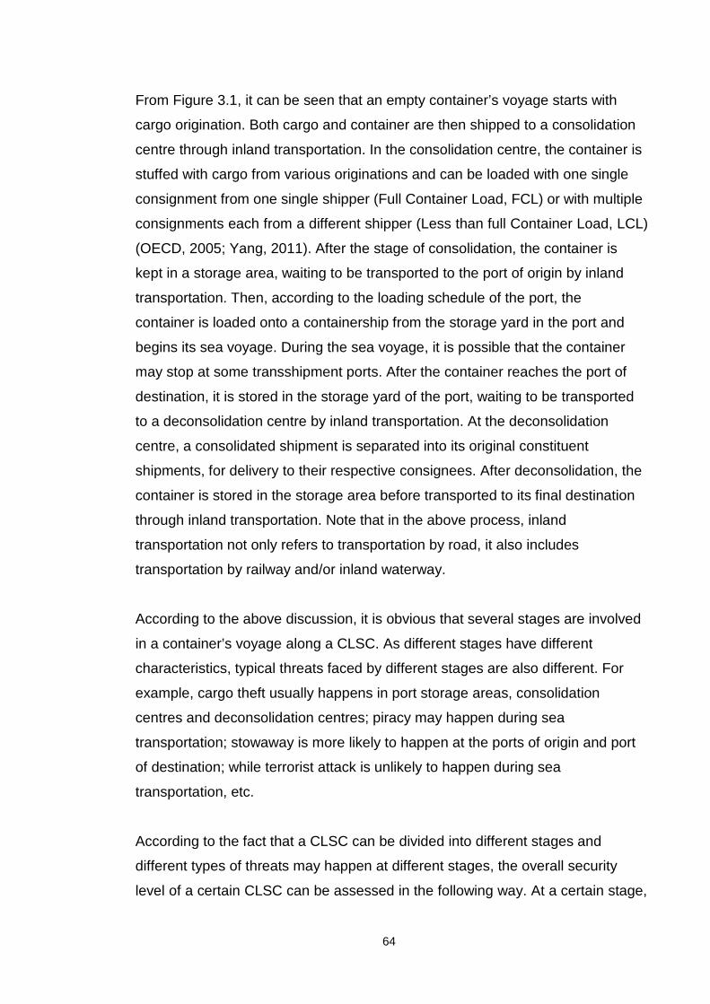
64
From Figure 3.1, it can be seen that an empty container’s voyage starts with
cargo origination. Both cargo and container are then shipped to a consolidation
centre through inland transportation. In the consolidation centre, the container is
stuffed with cargo from various originations and can be loaded with one single
consignment from one single shipper (Full Container Load, FCL) or with multiple
consignments each from a different shipper (Less than full Container Load, LCL)
(OECD, 2005; Yang, 2011). After the stage of consolidation, the container is
kept in a storage area, waiting to be transported to the port of origin by inland
transportation. Then, according to the loading schedule of the port, the
container is loaded onto a containership from the storage yard in the port and
begins its sea voyage. During the sea voyage, it is possible that the container
may stop at some transshipment ports. After the container reaches the port of
destination, it is stored in the storage yard of the port, waiting to be transported
to a deconsolidation centre by inland transportation. At the deconsolidation
centre, a consolidated shipment is separated into its original constituent
shipments, for delivery to their respective consignees. After deconsolidation, the
container is stored in the storage area before transported to its final destination
through inland transportation. Note that in the above process, inland
transportation not only refers to transportation by road, it also includes
transportation by railway and/or inland waterway.
According to the above discussion, it is obvious that several stages are involved
in a container’s voyage along a CLSC. As different stages have different
characteristics, typical threats faced by different stages are also different. For
example, cargo theft usually happens in port storage areas, consolidation
centres and deconsolidation centres; piracy may happen during sea
transportation; stowaway is more likely to happen at the ports of origin and port
of destination; while terrorist attack is unlikely to happen during sea
transportation, etc.
According to the fact that a CLSC can be divided into different stages and
different types of threats may happen at different stages, the overall security
level of a certain CLSC can be assessed in the following way. At a certain stage,
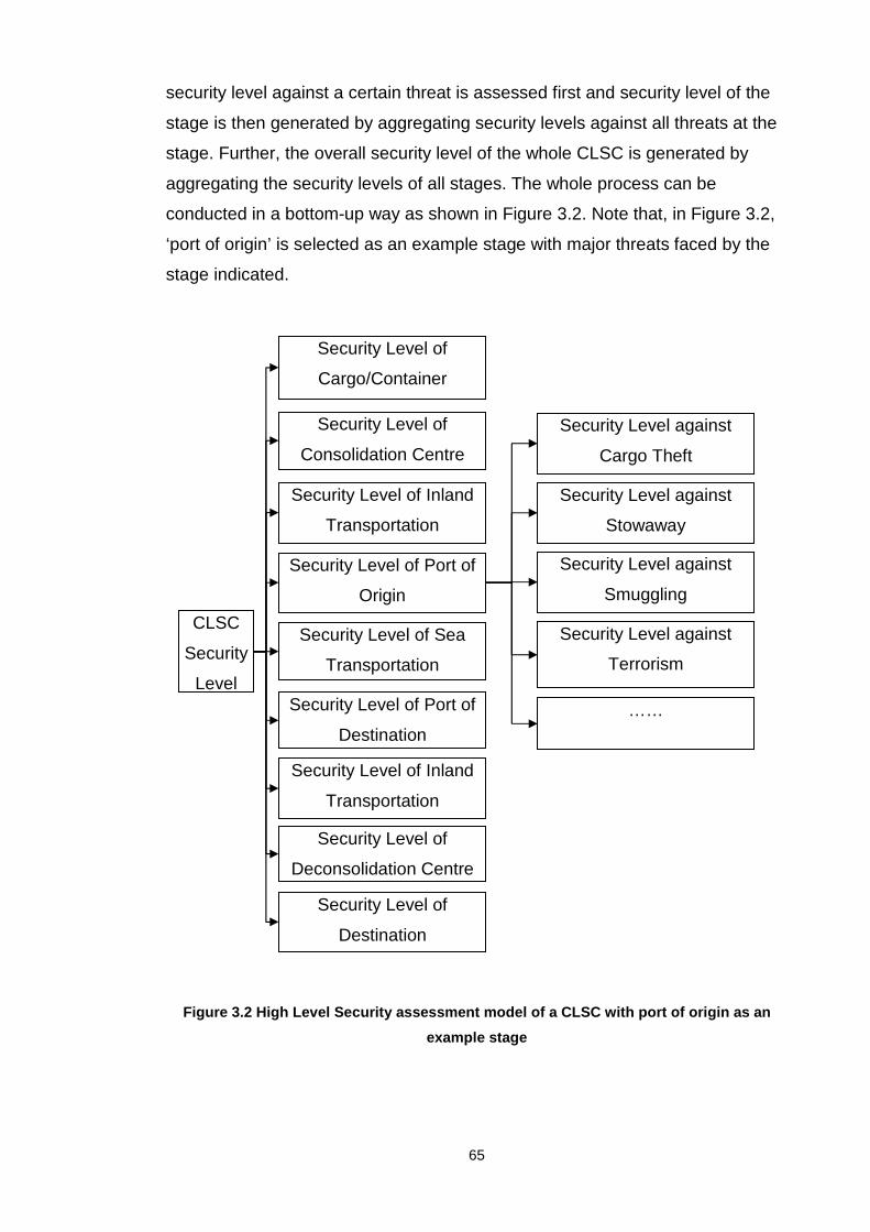
65
security level against a certain threat is assessed first and security level of the
stage is then generated by aggregating security levels against all threats at the
stage. Further, the overall security level of the whole CLSC is generated by
aggregating the security levels of all stages. The whole process can be
conducted in a bottom-up way as shown in Figure 3.2. Note that, in Figure 3.2,
‘port of origin’ is selected as an example stage with major threats faced by the
stage indicated.
Figure 3.2 High Level Security assessment model of a CLSC with port of origin as an
example stage
CLSC
Security
Level
Security Level of
Consolidation Centre
Security Level of Inland
Transportation
Security Level of Port of
Origin
Security Level of Sea
Transportation
Security Level of Port of
Destination
Security Level of Inland
Transportation
Security Level of
Deconsolidation Centre
Security Level of
Destination
Security Level against
Cargo Theft
Security Level against
Stowaway
Security Level against
Terrorism
Security Level against
Smuggling
……
Security Level of
Cargo/Container

66
3.2.2 Security representation and factors measureme nt
3.2.2.1 Security representation According to the above discussion, a certain stage in a CLSC against a certain
threat can be considered as a basic unit for CLSC security assessment. To
assess security level of a basic unit, the first question is how to represent
security. In other words, what are the basic components of security?
From the literature reviewed in Chapter 2, the concept of security considers not
only the likelihood of threat and the corresponding potential consequence, but
also the features of an organization under threat, in terms of how prevention,
detection and reaction activities regarding a threat are conducted. Therefore, in
addition to threat likelihood and potential consequence for risk modelling,
another component, the vulnerability of the affected organization, is considered
as a component for security representation. Therefore, security is represented
by 3 components in this thesis as follows:
• Threat Likelihood: probability or likelihood of the occurrence of a threat;
• Potential Consequence: the most severe impact on the affected
organization which may be caused by the threat. The impact can be
estimated according to a comprehensive review of the similar previous
security incidents and the current situation of the affected organization;
• Vulnerability: the features of the affected organization which can
influence (either increase or decrease) the likelihood of the occurrence of
the potential consequence after a threat has happened
As security is relevant to malicious harm, Threat Likelihood can be further
described by Intention of criminals and Capability Required for the criminals to
conduct criminal activities (Greenberg et al., 2006). Intention is the motivation of
criminals to launch a threat and is usually determined by potential benefits that
criminals can get if the threat is launched successfully, while the Capability
Required to launch the threat is related to skills and tools that criminals must
acquire to launch the threat. Based on the above interpretation, the Threat
Likelihood will be very high if criminals can get great benefits once the threat is
67
successfully launched and only basic skills and tools are needed to launch the
threat.
On the basis of the American National Standard for Security (ASIS, 2009), five
dimensions are proposed as follows to describe Potential Consequence in detail:
• Human Loss: physical harm to people involved in a CLSC, including
human death and human injuries;
• Financial Loss: monetary loss of the affected organization in a CLSC;
• Corporate Image Loss: reputation loss of the affected organization in a
CLSC, e.g., loss of customers;
• Economic Loss: monetary loss of the affected organizations’ partners
along the CLSC.This element can be used to reflect the impact of the
affected organization on other organizations along the same CLSC,
especially, when the security of a whole CLSC is assessed, this element
can be used to reflect the interactions among different organizations
involved in the CLSC;
• Environmental Loss: degradation to the quality of the environment or to
endangered species
As for Vulnerability, the features of the affected organization refer to both
Physical Features of the organization and Intervention Measures conducted by
relevant staff in the organization. Examples of Physical Features include
Historic Features, Employee Features, Facility Features etc., while Intervention
Measures may include Preventative Measures aiming at preventing potential
consequences from happening, Responsive Measures aiming at reducing the
impact of the consequences immediately after the consequences appear and
Recovery Measures aiming at helping the affected organization return to its
normal status after the consequences. Note that for the same affected
organization, the Vulnerability may be different against different threats.
The relation among the factors explained above can be summarized in Figure
3.3 as follows. Note that the security level of any basic unit for CLSC security

68
assessment, i.e., security level of any stage in a CLSC against any threat,
should be represented by the framework in Figure 3.3.
Figure 3.3 Framework to model security in a basic u nit for CLSC security assessment
From Figure 3.3, it can be seen that regarding a basic unit for CLSC security
assessment, components relevant to Threat Likelihood, Vulnerability and
Potential Consequence should be measured respectively. However, for some
basic units, i.e., for some stages along a CLSC against some threats, some of
the components in Figure 3.3 are too abstract to be measured directly.
Therefore, the components may need to be further decomposed into more
detailed factors according to the characteristics of specific basic units, and such
a decomposition process should continue until the factors after the
decomposition can be measured directly.
3.2.2.2 Measurement of factors: a general discussion As CLSC operates under complex environments, it is natural that factors
relevant to CLSC security assessment cannot be measured in a single fixed
way due to their different characteristics. In other words, the factors may need
to be measured in different ways such as qualitative terms, quantitative
numbers, categorized values, etc. In addition, subjective judgments and
incomplete information are also prevalent in CLSC security assessment, which
leads to different kinds of uncertainty in security assessment. Therefore, a
Security
Threat Likelihood
Vulnerability
Consequence
Intention
Capability Required
Physical feature
Intervention Measures
Cooperate Image
Financial Cost
Human Cost
Economic Cost
Environmental Cost
Preventative Measures
Responsive Measures
Employee Feature
Facility Feature
Historic Feature
Recovery Measures

69
framework which is capable of accommodating different forms of information
with different kinds of uncertainty is needed to measure the factors.
On the other hand, to accommodate different forms of information with different
kinds of uncertainty, belief distributions are introduced (Yang and Singh, 1994).
In general, to represent an assessment of a piece of evidence with uncertainty,
a set of mutually exclusive and collectively exhaustive assessment grades are
defined to provide a complete set of standards to describe the evidence, which
are represented by (3.1):
1 2, ,..., NH H H H= (3.1)
In (3.1), ( )1,2,...,nH n N∈ is the nth assessment grade, and it is assumed that
1nH + is preferable to nH for 1,2,..., 1n N∈ − . To represent the extent to which the
evidence can be described by each grade, a value ( )1,2,...,n n Nβ ∈ is attached
to each nH . Therefore, the assessment of the evidence E can be represented by
(3.2) as follows:
( ) ( ) ( ) ( ) 1 1 2 2, , , ,..., ,N NS E H H Hβ β β= (3.2)
In (3.2), ( )0 1,2,...,n n Nβ ≥ = and1
1N
ii
β=
≤∑ . The meaning of (3.2) can be
explained as: the evidence E can be described by grade ( )1,2,...,nH n N= with the
degree of nβ . If1
1N
ii
β=
=∑ , the assessment of E is said to be complete, and if
1
1N
ii
β=
<∑ , it is incomplete. Especially, 1
0N
ii
β=
=∑ denotes a total lack of information
regarding the assessment of E (Yang and Singh, 1994; Yang and Xu, 2002).
The expression in (3.2) is called as a belief distribution regarding E . With the
transformation methods introduced by Yang (2001), the most important
advantage of belief distribution is that it can accommodate different forms of
information, e.g., quantitative information, qualitative information, with different

70
kinds of uncertainty, e.g., uncertainty caused by fuzzy information, uncertainty
caused by incomplete information.
Therefore, belief distributions are considered as the framework to measure the
factors relevant to CLSC security assessment due to its capability to
accommodate different forms of information with different kinds of uncertainty,
and such a capability will be elaborated in detail in the following sections.
3.3 Model for security assessment of a port storage area in a CLSC against cargo theft
3.3.1 The hierarchical model
From the literature review, it is known that a CLSC faces various threats during
its operation. Among possible threats, although terrorism is of course a threat
with the most serious consequences, one of the most common threats to CLSC
security, however, is cargo theft (U.S. Maritime Administration, 2002), which
leads to about $40 billion direct cost every year, with indirect costs many times
higher worldwide (Eyefortransport, 2002). In addition to financial loss, cargo
theft may also lead to further economic loss and corporate image loss. If the
stolen cargo is hazardous (poisonous, explosive, radioactive, etc), the
consequence will even include human loss and environmental loss. The worst
situation is that a group of terrorists steal a certain amount of hazardous cargo
on purpose, and the stolen cargo is then used for terrorist activities. On the
other hand, with the consideration of criminals’ convenience, most cargo theft
occurs when cargo is at rest instead of in motion, and port is one of the most
important places where cargo is at rest during their voyage along a CLSC.
Therefore, security assessment of a port storage area along a CLSC against
cargo theft becomes essential.
The general framework to model the security of a basic unit for CLSC security
assessment in Figure 3.3 can be refined for the security assessment of a port
storage area along a CLSC against cargo theft. Specifically, according to the
characteristics of cargo theft in a port storage area, the factors at the bottom
level of the hierarchical structure in Figure 3.3 should be either measured
directly in an appropriate way, or measured through a proxy attribute, or

71
decomposed into more specific and measureable factors. The above process is
discussed in detail as follows:
In Figure 3.3, the factor Intention refers to the motivation of criminals to conduct
a cargo theft, which is usually determined by potential benefits that criminals
can get if cargo theft is successfully conducted. Criminals will be more willing to
conduct a theft if the cargo stolen is of more interest to them. Therefore, under
the context of cargo theft, Intention is closely related to a proxy attribute: cargo
value. Note that cargo value doesn’t only refer to its monetary value. For
example, hazardous cargo may not be expensive in monetary term, but if
criminals are terrorists, who want to launch a terrorist attack using the
hazardous cargo, the hazardous cargo may be of great value to the criminals.
The factor Capability Required refers to skills or tools that criminals must
acquire to conduct a theft, which is related to both the preventative capability of
the port and the type of cargo. If the port is well protected, criminals may not be
able to conduct a theft successfully without inside help, and if a cargo is huge,
e.g., a heavy mechanical machine, criminals may need a truck or even a crane
to move the cargo. In both cases, Capability Required to successfully conduct
cargo theft is very high. Therefore, Capability Required is affected by the
combination of the Preventative Capability of the port and the Magnitude of
Cargo stored in the port.
As for Historic Feature, it refers to frequency of cargo theft happened in the port
storage area in history, while Employee Feature is reflected by whether there
are any current employees conducted or involved in any cargo theft before.
Facility feature can be described by Hardware Feature and Software Feature.
Software Feature of a port storage area mainly refers to the features of
information system operated in the port. Under the context of cargo theft
prevention, Software Feature in a port is represented by its capability to detect,
prevent and react to unauthorized access or breaches to the information
system. Hardware Feature of a port storage area is composed of the features of
Control Facility and the features of Monitor Facility. Control Facility can then be

72
further divided into Access Control System, Alarm System and Connection
between them, i.e., whether the alarm system can be triggered when the access
control system is breached. To assess the performance of an Access Control
System, its Coverage, Capability and Robustness need to be measured. While
for an Alarm System, its Capability and Robustness are considered as
performance criteria. The most typical Monitor Facility is CCTV Facility, and
criteria for assessing whether it is good enough to prevent cargo theft in a port
storage area include its Coverage, Media used to record images and Retention
Period of images kept in the CCTV Facility. In addition to CCTV Facility,
Lighting Facility should also be considered as a component of Monitor Facility.
For a Lighting Facility, its Coverage and Capability can be selected as two
criteria to measure its performance.
Preventative Measures refer to the measures preventing consequence of cargo
theft from happening, which can be achieved by Managerial Measures and
Operative Measures. Managerial Measures are the measures relevant to
policies, regulations or requirements followed or developed by a port to maintain
its security against cargo theft in storage areas while Operative Measures refer
to actions taken by staff in a port to protect cargo from being stolen.
More specifically, Managerial Measures include Regulations and Management
on Regulations. Regulations can be decomposed into the following aspects:
General regulations regarding overall security, Regulations regarding access
control and Regulations regarding procedure control. On the other hand,
Management on Regulations concerns whether the execution status of the
regulations is Monitored and Audited and whether the regulations are Updated
periodically. For General regulations regarding overall security, the following
two aspects are considered: whether the ISPS Code is applied in a port and
whether there are regulations on how to create and maintain security culture in
a port. In addition, Regulations on access control should consider the access
control towards the following three targets: current employees, terminated
employees and visitors. Moreover, procedures for stuffing, loading and
unloading as well as procedures for security incident reporting should be
regulated by Regulations regarding procedure control.
73
Operative Measures regarding port security against cargo theft include the
following categories: Operations relevant to access control, Operations relevant
to employee training and auditing, Operations relevant to records, Operations
relevant to security related equipments, and Operations relevant to other
issues. Each category of the above operations can be further divided into more
detailed levels as follows:
• Operations relevant to access control include application of Photo-ID
badge and application of Key/key card
• Operations relevant to employee training and auditing include Training of
employees and Auditing the status of employees regularly
• Operations relevant to records include Keeping of records, Protection of
records and Management of records. Specifically, records kept are
composed of Security system related records and Employee related
records, in which Security system related records refer to both Logs of
alarm systems and Logs of access control systems while Employee
related records include Records of emergency contacts, Records of
employee training, and Records of terminated employees in recent 3
years
• Operations relevant to security related equipments refer to Control of
cargo-handling equipment, Test/maintenance/repair for security systems
and the application of Uninterruptible Power Supply (UPS) or other forms
of emergency power supply of security systems
• Operations relevant to other issues include Cargo Inspection,
Vulnerability Assessment and Guarding/patrolling. For Cargo Inspection,
it refers to both Inspection on containers and Inspection on trash
Apart from Preventative Measures, another category of Intervention Measures
are Responsive Measures. Responsive Measures are influenced by the
following factors: Responsive Activity and Responsive Facility. Responsive
Activity mainly refers to activities relevant to contingency plans, including
development, update and drill of contingency plans. Responsive Facility
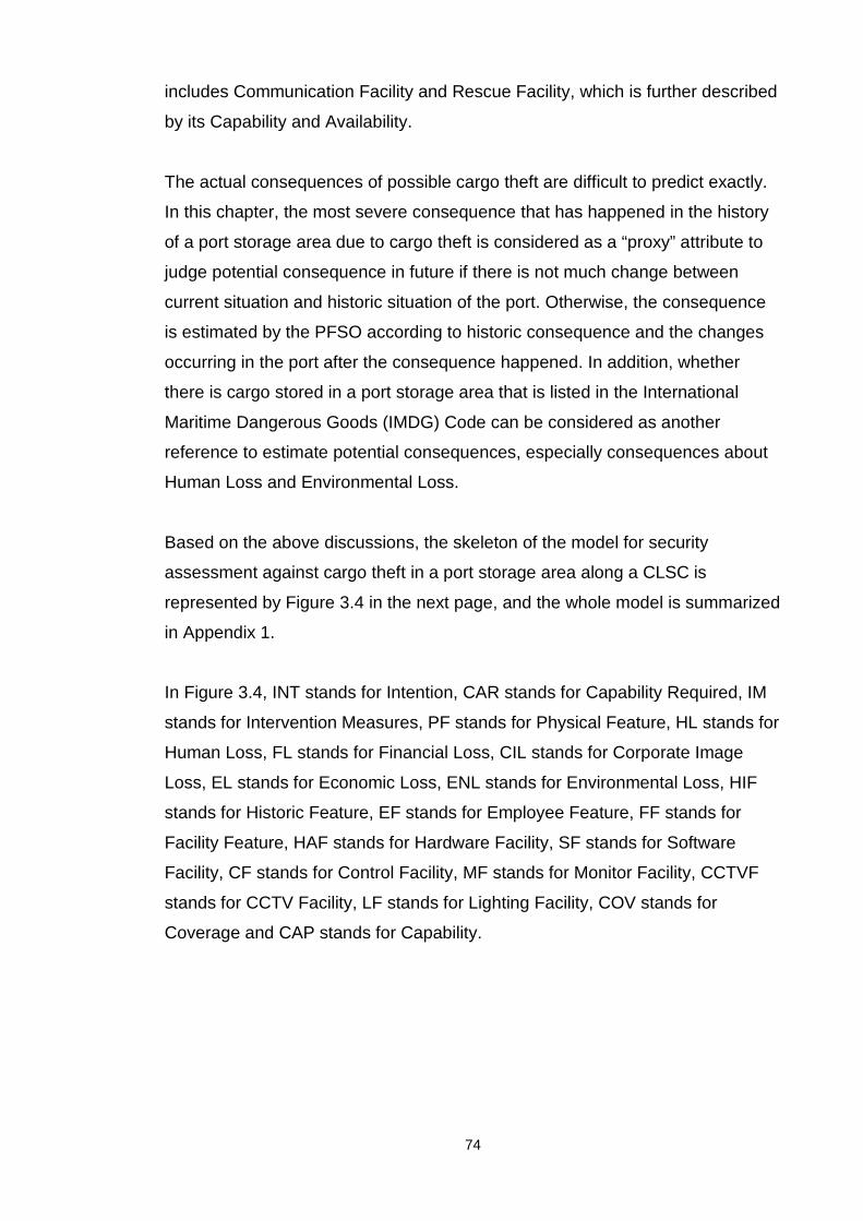
74
includes Communication Facility and Rescue Facility, which is further described
by its Capability and Availability.
The actual consequences of possible cargo theft are difficult to predict exactly.
In this chapter, the most severe consequence that has happened in the history
of a port storage area due to cargo theft is considered as a “proxy” attribute to
judge potential consequence in future if there is not much change between
current situation and historic situation of the port. Otherwise, the consequence
is estimated by the PFSO according to historic consequence and the changes
occurring in the port after the consequence happened. In addition, whether
there is cargo stored in a port storage area that is listed in the International
Maritime Dangerous Goods (IMDG) Code can be considered as another
reference to estimate potential consequences, especially consequences about
Human Loss and Environmental Loss.
Based on the above discussions, the skeleton of the model for security
assessment against cargo theft in a port storage area along a CLSC is
represented by Figure 3.4 in the next page, and the whole model is summarized
in Appendix 1.
In Figure 3.4, INT stands for Intention, CAR stands for Capability Required, IM
stands for Intervention Measures, PF stands for Physical Feature, HL stands for
Human Loss, FL stands for Financial Loss, CIL stands for Corporate Image
Loss, EL stands for Economic Loss, ENL stands for Environmental Loss, HIF
stands for Historic Feature, EF stands for Employee Feature, FF stands for
Facility Feature, HAF stands for Hardware Facility, SF stands for Software
Facility, CF stands for Control Facility, MF stands for Monitor Facility, CCTVF
stands for CCTV Facility, LF stands for Lighting Facility, COV stands for
Coverage and CAP stands for Capability.
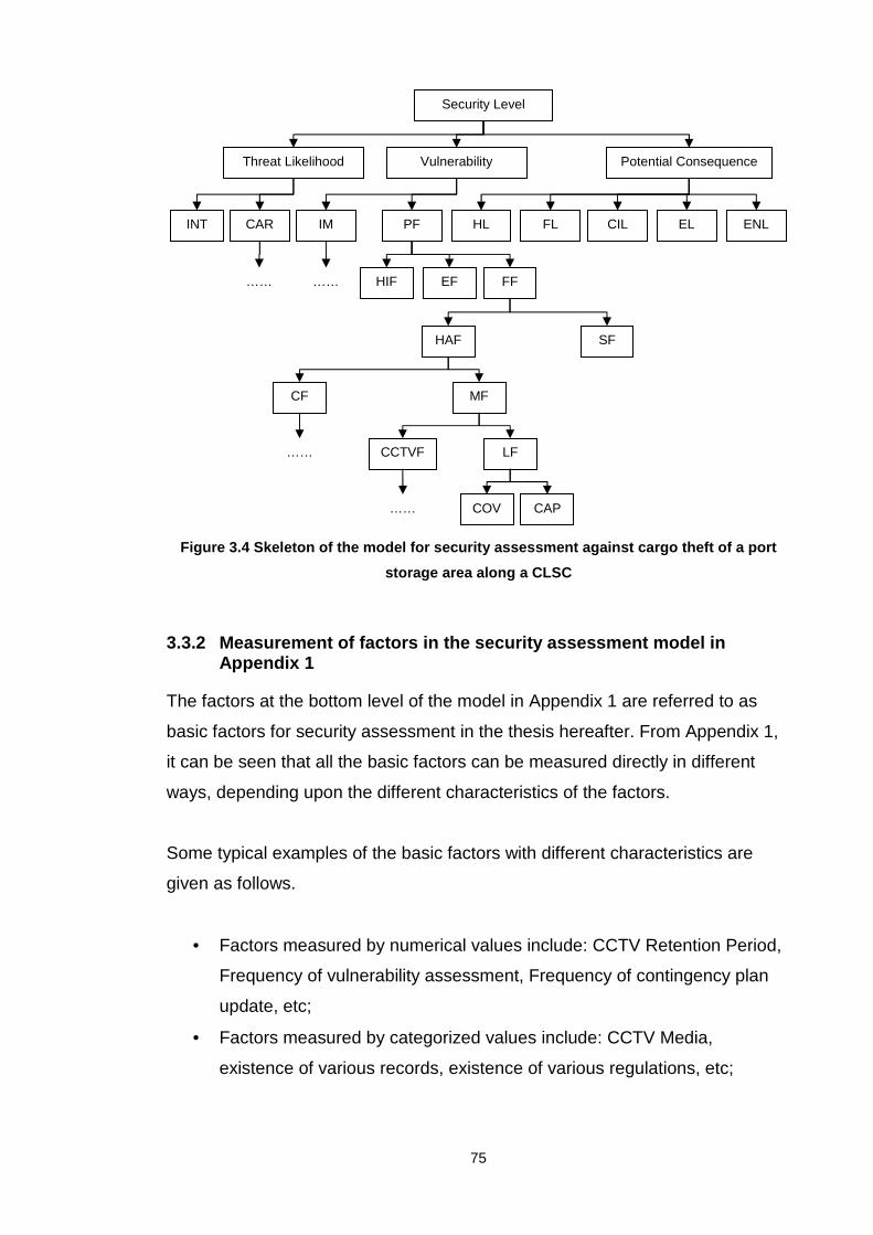
75
Figure 3.4 Skeleton of the model for security asses sment against cargo theft of a port
storage area along a CLSC
3.3.2 Measurement of factors in the security assess ment model in Appendix 1
The factors at the bottom level of the model in Appendix 1 are referred to as
basic factors for security assessment in the thesis hereafter. From Appendix 1,
it can be seen that all the basic factors can be measured directly in different
ways, depending upon the different characteristics of the factors.
Some typical examples of the basic factors with different characteristics are
given as follows.
• Factors measured by numerical values include: CCTV Retention Period,
Frequency of vulnerability assessment, Frequency of contingency plan
update, etc;
• Factors measured by categorized values include: CCTV Media,
existence of various records, existence of various regulations, etc;
Security Level
Threat Likelihood Vulnerability Potential Consequence
INT CAR IM PF CIL EL
…… HIF EF FF
HAF SF
ENL
CF MF
CCTVF LF ……
COV CAP ……
HL FL
……
76
• Factors measured by subjective terms include: CCTV Coverage, CCTV
Capability, Robustness of alarm systems, Control on cargo handling
equipments, etc.
In addition to the above categories of measurement, it is natural that information
about some factors may be incomplete because of the incapability or high cost
to collect the information or the information is not available at all.
As discussed in Section 3.2.2, in order to accommodate information in various
forms with different kinds of uncertainty, belief distributions are used to model
all the factors in the security assessment model in Appendix 1. Before the belief
distributions can be applied, a set of grades to describe the factors or a set of
possible values the factors may take need to be defined first, such as ‘Long’,
‘Moderate’ and ‘Limited’ for CCTV Retention Period, ‘High’, ‘Moderate’ and
‘Low’ for CCTV Capability, and ‘Video Cassette Recorder (VCR)’ and ‘Digital
Video Recorder (DVR)’ for CCTV Media, etc. Based on the grades or values
defined, belief distributions are generated to describe the factors in different
ways according to the characteristics of the factors:
• For quantitative factors, the value corresponding to each grade should be
specified and the value taken by the factor should be transformed to a
belief distribution using the transformation methods proposed by Yang
(2001). For example, for the factor of Frequency of vulnerability
assessment, it can be described by 3 grades: ‘Frequent’, ‘Standard’ and
‘None’. To define the meaning of each grade, relevant regulations should
be reviewed. In the UK, it is required by TRANSEC that for each port,
vulnerability assessment should be conducted at least once every 3
years. Therefore, for UK ports, the grade ‘Frequent’ can be defined as
‘vulnerability assessment is conducted once every year’, ‘Standard’ can
be defined as ‘vulnerability assessment is conducted once every 3
years’, and ‘None’ means ‘there is no vulnerability assessment
conducted in the port’. If a port in the UK conducts vulnerability
assessment once every 2 years, based on the transformation method
(Yang, 2001), the Frequency of Vulnerability Assessment of the port can
77
be represented by (Frequent, 0.5), (Standard, 0.5), (None, 0). As there
may be difference among regulations in different countries, for ports in
different countries, the explanation for the same grade of the same basic
factor may be different;
• For a categorized factor, the degree attached to a possible value is either
1 or 0, indicating whether the factor can be described by the value or not.
For example, for the factor of CCTV Media, the value it can take is either
VCR or DVR, and the belief distributions to describe CCTV Media is
either (VCR, 0), (DVR, 1) or (VCR, 1), (DVR, 0);
• For subjective factors, the degree attached to a certain term is between 0
and 1, indicating the extent to which a basic factor is described by the
subjective term. One of the examples for this kind of factors is
Robustness of Alarm System, which can be described by the grades of
‘Robust’ and ‘Not Robust’. Depending upon the reality of a port and the
judgment of its PFSO, Robustness of Alarm System can be described by
a belief distribution such as (Robust, 0.9), (Not Robust, 0.1), meaning
that the alarm system in the port storage area is robust in general, but
occasionally there is still false alarm.
In addition to its capability of accommodating different forms of information,
belief distribution can also accommodate different kinds of uncertainty, and the
following example shows its capability of accommodating uncertainty caused by
incomplete information. CCTV system plays an important role to prevent cargo
theft in a port storage area. To assess the capability of a CCTV system in an
organization along a CLSC, a security officer may state that the CCTV
Capability is ‘High’ to a degree of 80%, ‘Moderate’ to a degree of 10% and ‘Low’
to a degree of 0%. In the statement, ‘High’, ‘Moderate’ and ‘Low’ are the grades
used to describe CCTV Capability, and 80%, 10% and 0% are degrees of belief,
representing the extent to which CCTV Capability is assessed to the
corresponding grades. The statement means that in the security officer’s
opinion around 80% of the CCTV cameras in the port are operating with ‘High’
capability whilst around 10% of them are operating with ‘Moderate’ capability.
The statement can be represented using the following belief distribution:
E(CCTV Capability)=(High, 0.8), (Moderate, 0.1),(Low, 0), where E(CCTV
78
Capability) represents the assessment of the CCTV Capability. Note that the
sum of 80%, 10% and 0% is 90%, less than 100%, which indicates that this
assessment is incomplete. A possible explanation about such an incomplete
assessment is that there may be too many CCTV cameras operating in the port
and the security officer does not have full knowledge about the capability of
each CCTV camera and thus he is not 100% sure about the capability of all
cameras in the port. However, he can update his judgment by checking all
cameras in the port if it is feasible.
A full list of assessment grades or possible values for all the basic factors is
given in Appendix 2, with the explanation of each grade or value provided.
On the other hand, for non-basic factors in the security assessment model in
Appendix 1, i.e., the factors which are not at the bottom level of the model, the
corresponding grades are listed in Appendix 3. Since the meanings of non-basic
factors are not as specific as basic factors, there is no specific explanation of
the grades used to describe the non-basic factors listed in Appendix 3.
3.4 Case study
3.4.1 Case background
In order to validate the security assessment model developed in this chapter for
a port storage area along a CLSC against cargo theft, a questionnaire was
designed to collect PFSOs’ opinions on the basic factors in the model in
Appendix 1 according to the real situations of their ports. The questionnaire,
which is listed in Appendix 4, was sent to 15 different ports in the UK and China,
and there are 9 responses to the questionnaire, among which 5 sets of valid
data are collected. Among the 5 ports which provided valid response to the
questionnaire, 2 interviews were conducted with PFSOs in the UK and China
respectively to collect further information regarding their opinions on the security
assessment model and the real situation of their own ports.

79
In the following case study, the data collected from a port in China is used to
illustrate the applicability of the security assessment model in Appendix 1 in
detail.
Specifically, the port handles more than 5 million Twenty-feet Equivalent Units
(TEUs) every year. To ensure security, it has assigned a dedicated security
team and developed a set of security measures including a set of effective
contingency plans in place. Several internationally recognized security codes,
initiatives and programs are applied in the port, such as ISPS Code issued by
IMO, CSI, C-TPAT, Operation Safe Commerce (OSC) and Secure Freight
Initiative (SFI) issued by DHS, etc.
3.4.2 Measurement of factors according to real info rmation collected
To model the information collected from questionnaire and the interview
followed, belief distributions are used. Some typical examples are listed as
follows.
• Information measured by subjective terms: Regarding Regulations to
create security culture in the port, the PFSO stated that whilst a set of
regulations are developed to help create security culture, one of the
current problems concerned by him is the inadequate emphasis on
security in many employees’ minds although the daily security activities
are conducted in a routine way. This statement shows that there are
regulations for creating security culture but only some employees can
realize the importance of security for port operation, although employees
are doing what they are required to do for maintaining port security. By
analyzing the statement of the PFSO, and according to the explanation
of the grades/referential values regarding Regulations to create security
culture in Appendix 2, the assessment of the port on Regulations to
create security culture can be represented by the following belief
distribution (Effective, 0.1), (Not Effective, 0.9), (None, 0)
• Information measured by numerical values. In the port, the image of the
CCTV system is kept for 45 days. According to the definitions of
grades/referential values regarding CCTV Retention Period listed in
80
Appendix 2, 45 days of CCTV Retention Period is in the middle of ‘Long’
and ‘Medium’ and therefore can be represented by the belief distribution
(Long, 0.5), (Medium, 0.5), (Short, 0) according to the transformation
techniques (Yang, 2001)
• Information measured by categorized values. In the port, the content,
time, venue, and participants of every training course organized for
employees are well recorded and documented. The assessment of the
Records on employee training can thus be represented by the belief
distribution (Yes, 1), (No, 0).
In a similar way, all the other basic factors in the security assessment model in
Appendix 1 can be measured by belief distributions according to the
explanations of each grade/referential value to describe the factors and the
information collected from questionnaire and interview with the PFSO.
After the information regarding basic factors in the security assessment model
in Appendix 1 has been collected and measured by belief distributions, the next
step is to use RIMER to assess the security level of the port against cargo theft.
And this is the main content of the next chapter.
3.5 Conclusion
Facing the fact that CLSC is a predominant way for world cargo transportation
and that CLSC is subject to various threats during its operation due to its
complexity and vulnerability, a general model, which is based on a typical
voyage of a container along a CLSC and threats faced by the container in each
stage along a CLSC, is proposed in this chapter to facilitate analytical security
assessment of a general CLSC. To validate the applicability of the security
assessment model for general CLSCs, it is then further refined for security
assessment in a port storage area along a CLSC against cargo theft after
relevant factors are identified and organized hierarchically, and belief
distributions are used to measure the basic factors in the refined model to
accommodate different forms of information contained in the factors and
different kinds of uncertainty involved in the factors.
81
Compared with other research on CLSC security, the model proposed in this
chapter has several features which are summarized as follows. 1) The model
identifies and organizes CLSC security-related factors in a structured way and
thus provides a basis for analytical security assessment, which enriches the
existing descriptive research on CLSC security. 2) The model is flexible to
accommodate information in different forms, such as quantitative, qualitative,
categorized, etc. This feature is important in security assessment in CLSC as
there are many factors with different features in the assessment process, and
all the factors should be accommodated in a model in a unified way. 3) The
model is capable of dealing with different kinds of uncertainty. This feature is
also vital in CLSC security assessment as uncertainty, either caused by
subjectivity or caused by incompleteness, are inevitable in the assessment
process.
However, developing a model for security assessment is only a starting point for
security analysis, and it is also necessary to conduct security assessment and
to investigate how to make appropriate decisions based on assessment results,
such as how to effectively allocate limited resources to improve the security
level of a certain CLSC. The above 2 aspects will be discussed in the
subsequent chapters of the thesis.

82
4 Chapter 4 Generation of belief degrees in Belief Ru le Bases and security assessment of CLSC using RIMER
Abstract
Based on the security assessment model developed in Chapter 3, RIMER can
be applied to generate security assessment result of a general CLSC as well as
a certain stage along a CLSC against a certain threat. As BRBs are the basis
for the application of RIMER, to ensure reliability and rationality of security
assessment results, the parameters of BRBs, especially belief degrees in BRBs
should be generated with minimum bias and inconsistency. In this chapter, a
new process is proposed to generate belief degrees in BRBs for the security
assessment model proposed in Chapter 3 regarding a port storage area along a
CLSC against cargo theft. Based on the BRBs, the security assessment is then
conducted by RIMER.
4.1 Introduction
As revealed in previous discussions, due to the complexity of CLSC operation,
the factors which can influence CLSC security have different inherent features
and thus should be measured by different forms of information. In addition,
different kinds of uncertainty are also inevitable in security assessment. On the
other hand, with the incorporation of belief distributions, RIMER has the
capability of accommodating and handling different forms of information with
different kinds of uncertainty. Therefore, RIMER is selected as the tool for
CLSC security assessment. However, how to extract knowledge from experts to
generate belief degrees in BRBs and minimize bias and inconsistency during
the generation process remains an open and domain specific research question
without a generic solution currently. Moreover, as discussed in Chapter 2, one
of the features of CLSC is that there is limited historic data available for CLSC
security analysis, which makes it impractical to use parameter training to reduce
bias and inconsistency involved in the process to generate belief degrees in
BRBs. It is therefore important to develop an effective and feasible method to
initialize BRB with the capability of minimizing bias and inconsistency.
83
In this chapter, a new process is proposed to generate belief degrees in BRBs
based on knowledge extracted from experts, with the aim to reduce bias and
inconsistency involved in the generation process. After BRBs are generated, the
security assessment of port storage areas in CLSCs against cargo theft is
conducted based on real data collected.
4.2 Introduction of Belief Rule Base and generation of belief degrees in Belief Rule Bases
4.2.1 Introduction to Belief Rule Base
BRB is built on the basis of traditional rule base, the kth rule in which can be
represented as:
kR : IF 1A is11
kpA AND 2A is
22k
pA AND … AND MA isM
kMpA , THEN D is jD . (4.1)
In (4.1), 1 2, ,..., MA A A are the antecedents of the rule base, M is the number of
antecedents,i
kipA ( )1,2,..., , 1,2,...,i ii M p M∈ ∈ is the ip th referential value
taken by iA or the ip th grade used to describe iA in the kth rule, iM is the number
of referential values or grades regarding iA , and D is the consequence of the rule
base while ( )1,2,...,jD j N∈ is the jth referential value or the jth grade regarding
D in the kth rule. In addition, 1 2, ,..., MA A A can be called as the packet
antecedent of the rule base, while 1 21 2, ,...,
M
k k k kp p MpA A A A= is the packet
antecedent of the kth rule in the rule base.
Representing the relation among 1 2, ,..., MA A A and D by (4.1) may lead to two
major limitations: 1) as the consequence is represented by a single referential
value taken by D , it cannot reflect the minor difference among the packet
antecedents of different rules, i.e., different packet antecedents in different rules
with minor difference may lead to the same consequence; 2) in complex
applications, the relation among 1 2, ,..., MA A A and D are always uncertain, such
uncertainty of the relation cannot be denoted by (4.1) either.

84
In order to overcome the limitations, BRB is proposed (Yang, et al., 2006).
Different from traditional rule base, in BRB, the consequence is not represented
by a single referential value, but a distribution of belief degree on each
referential value that can be used to describe the consequence.
Specifically, the kth rule in a BRB corresponding to (4.1) can be represented as
follows:
kR : IF 1A is11
kpA AND 2A is
22k
pA AND … AND MA isM
kMpA , THEN D is
( ) ( ) ( ) 1 1 2 2, , , ,..., ,k k N NkD D Dβ β β , with rule weight kθ and antecedent weight
( )1,2,...,kj j Mδ = for antecedent jA in the kth rule (4.2)
In (4.2), ( )1,2,..., ,0 1ik iki Nβ β= ≤ ≤ is the degree to which iD is used to describe
consequence D in the kth rule, kθ reflects the relative importance of the kth rule
among the rules in the whole rule base, kjδ reflects the relative importance of the
jth antecedent in the kth rule. If the knowledge on the relation among
1 2, ,..., MA A A and D when iA is described by ( )1,2,...,iip i iA p M∈ for all
1,2,...,i M= is complete,1
1N
iki
β=
=∑ , otherwise, 1
1N
iki
β=
<∑ .
The rule represented by (4.2) is called a belief rule and the rule base containing
belief rules is called a BRB. In a BRB, both the difference among packet
antecedents of different rules and the uncertainty existing in the knowledge
regarding the relation among antecedents and consequence can be reflected by
different belief distributions assigned to the consequence of different belief
rules. In addition, with the introduction of antecedent weights and rule weights,
the relative importance of each antecedent of the BRB and that of each rule in
the BRB can be reflected conveniently.
From the above discussion, it can be seen that in a BRB, the basic element is a
belief rule, and a typical belief rule is represented by (4.2). In essence, a belief
rule actually builds a relation among the antecedents 1 2, ,..., MA A A and the
85
consequence D . Specifically, the belief rule in (4.2) can be explained as: on the
condition that jA takes the referential value ofjjpA for all 1,2,...,j M= ,
consequence D can be described by ( )1,2,...,iD i N= with the belief degree of iβ .
From the above explanation, it can be seen that, the belief degree that
consequence D being described by a certain referential value is conditional on
the referential values taken by different antecedents. This conditional
relationship can also be described from another angle: conditional probability.
On the other hand, Bayesian Network (BN) is a typical tool to model conditional
probabilities. As such, a relation can be built between BRB and BN. Specifically,
BRB models relation among its antecedents and consequence by belief
degrees while BN models relation among parent node and its child node(s) in
the network by Conditional Probability Tables (CPTs), and the relation between
belief degrees in BRBs and CPTs in the corresponding BNs will be explained in
detail after a brief introduction of BN is given.
4.2.2 A brief introduction to Bayesian Network
BN is a Directed Acyclic Graph (DAG), in which a node stands for a factor under
concern, and a directed arc, pointing from a parent node to a child node in a BN,
represents the causal relation between the two nodes (Pearl, 1988).
In a BN, each node is associated with a probability table. A probability table for
a node without any parent node gives the probability distribution of states which
are used to describe the node. A probability table for a node with parent nodes
presents the probability distribution of the node’s state conditional on every
possible state combination of its parent nodes, and in this case, the probability
table is called a CPT.
For a BN, one of its most important capabilities is that the probability distribution
of each node can be updated when the probability distribution of any node in
the network is changed. In other words, when new information or observation of
any factor is available, the information or judgment of other factors will be
updated in an automatic and instant way, and the update scheme of BN is the
Bayes Theorem, which is represented by (4.3) as follows:

86
( ) ( ) ( )( )
P B A P AP A B
P B= (4.3)
From (4.3), it can be seen that, with the emergence of new information or new
observation regarding Node B, the prior probability of Node A, ( )P A , is updated
to the corresponding posterior probability ( )P A B .
4.2.3 Relationship between Belief Rule Base and Bay esian Network
Generally, any complex BN can be decomposed into several fragments, each of
which has one child node with its parent node(s). In this chapter, the fragment
with one child node with its parent node(s) is called a ‘basic BN fragment’. A
typical basic BN fragment is presented in Figure 4.1 as follows.
Figure 4.1 A basic BN fragment
In Figure 4.1, child node D has M parent nodes, i.e., 1 2, ,..., MA A A . Suppose node
D can be described by N different states, i.e., 1 2, ,..., ND D D , while node jA
( )1,2,...,j M∈ can be described by jM different values, namely, 1 2, ,...,jj j jMA A A .
As an arc in a BN between a parent node and a child node represents the
casual relationship between them, and such a causal relationship can also be
represented by belief rules in a BRB, we can naturally translate the basic BN
fragment in Figure 4.1 into a BRB, with the kth belief rule represented by (4.2).
Specifically, the parameters in the belief rule in (4.2) can be explained from the
perspective of BN as follows: jjpA ( )1,2,..., , 1,2,...,j jj M p M∈ ∈ is the jp th
D
A1 A2 …… AM

87
state of node jA , iD ( )1,2,...,i N= is the ith state of node D , and ( )1,2,...,ik i Nβ =
equals to the probability that node D is in the state of iD under the condition
that jA ( )1,2,...,j M= is in the state of jjpA ( )1,2,...,j jp M∈ for all 1,2,...,j M= ,
i.e.,
( )1 21 1 2 2| , ,...,
Mik i p p M MpP D D A A A A A Aβ = = = = = (4.4)
On the other hand, as introduced previously, (4.2) can be explained from the
perspective of BRB as follows: in the kth rule of a BRB, when jA takes the
referential value of jjpA for all 1,2,...,j M= , the consequent D can take the value
of iD with the belief degree of ikβ .
From the above illustration, the relationship between a BRB with the kth rule
represented by (4.2) and a basic BN fragment represented by Figure 4.1 can be
summarized as follows:
1) Each antecedent in the BRB is corresponding to a parent node in the
basic BN fragment, and the packet antecedent of the kth belief rule in the
BRB is corresponding to a specific state combination of the parent nodes
in the basic BN fragment;
2) The consequence of the BRB is corresponding to the child node in the
basic BN fragment, and the referential values in the consequence of the
BRB is corresponding to the states of the child node in the basic BN
fragment;
3) The belief degree assigned to each referential value in the consequence
of the kth belief rule in the BRB is corresponding to the probability of
each state of the child node conditional on the specific state combination
of the parent nodes specified in 1) in the basic BN fragment;
Therefore, we can find that the belief degrees in the BRB with the kth belief rule
represented by (4.2) are corresponding to the probabilities in the CPT of the
basic BN fragment as represented by Figure 4.1.

88
Note that, since each antecedent ( )1,2,...,jA j M= in (4.2) can take jM different
values, there are 1
M
jj
M=
∏ possible combinations for packet antecedent from the
perspective of BRB, and each combination will induce a belief rule. Therefore,
the BRB corresponding to the basic BN fragment in Figure 4.1 has 1
M
jj
M=
∏ belief
rules.
4.2.4 Generation of belief degrees in BRBs
From the above discussion, we can see that in order to find out the relation
between packet antecedent and consequence in the BRB with the kth rule
represented by (4.2) from a BRB view, we can figure out the relationship
between parent nodes and their common child node in the basic BN fragment
represented by Figure 4.1 from a BN view.
As the relation between packet antecedent and consequence in a BRB is
represented by belief degrees in the consequence, and the relation between
parent nodes and their common child node in a basic BN fragment is
represented by the corresponding CPT, according to the relationship between
BRB and BN analyzed in previous section, to generate belief degrees in a BRB,
the probabilities in the CPT of the corresponding basic BN fragment should be
generated, i.e., the probability of each state of the child node conditional on
each state combination of its parent nodes in the basic BN fragment should be
generated.
4.2.4.1 Current methods for conditional probability generation in BNs For generation of conditional probabilities in BNs, the most classic approach is
the noisy OR model (Pearl, 1988) and its generalizations (Diez, 1993; Cozman,
2004). However, such a method can only handle the cases where the states of
nodes are binary and the parents of nodes are assumed to be independent of
each other. In (Lemmer and Gossink, 2004) and (Das, 2004), the definition of
‘compatible’ is proposed in order to release the assumption of independence
and the restriction on the binary values and to reduce the burden of

89
computation if there is a large amount of nodes. However, for generation of
belief degrees in BRBs, the definition of ‘compatible’ is not practical since every
state combination of parent nodes is possible. In addition, Das’s approach is
based on experts’ direct estimation on the conditional probabilities which may
inevitably involve subjectivity and bias, leading to unreliability and inconsistency
in the estimation (Das, 2004). Monti and Carenini proposed another way to
generate conditional probabilities using pair-wise comparisons (Monti and
Carenini, 2000). The idea of this approach can be traced back to Schocken’s
work (Schocken, 1993). In pair-wise comparison, experts only need to
encounter two states instead of all the states of a node at a time when they give
their judgments on the states’ probabilities. In this way, the bias of judgments
could be reduced significantly and the consistency of judgments could be
maintained. However, Monti and Carenini (2000) only generated the conditional
probabilities of a node with a single parent, while for belief degree generation, it
is rare that there is only one antecedent in a BRB.
From the above introduction, it can be seen that there is a need to develop a
new process to generate CPTs for BNs with minimum bias and inconsistency
involved, and further to generate belief degrees in corresponding BRBs.
4.2.4.2 Proposed method for CPT generation in BNs and belief degrees generation in BRBs
The discussion on CPT generation is based on Figure 4.1, and correspondently,
the aim is to generate the probability that D takes the value of ( )1,2,...,iD i N∈
conditional on all possible state combinations of its parent node 1 2, ,..., MA A A , i.e.,
( )1 2, ,...,i MP D D A A A= , with minimum bias and inconsistency involved in the
generation process.
According to the number of parent nodes and the number of different states
which are used to describe each parent node, there may be a large number of
state combinations, which makes it very difficult, if not impossible, to figure out
the difference among each state combination of the parent nodes and the
impact of such difference on the probability of the states used to describe the
child node.
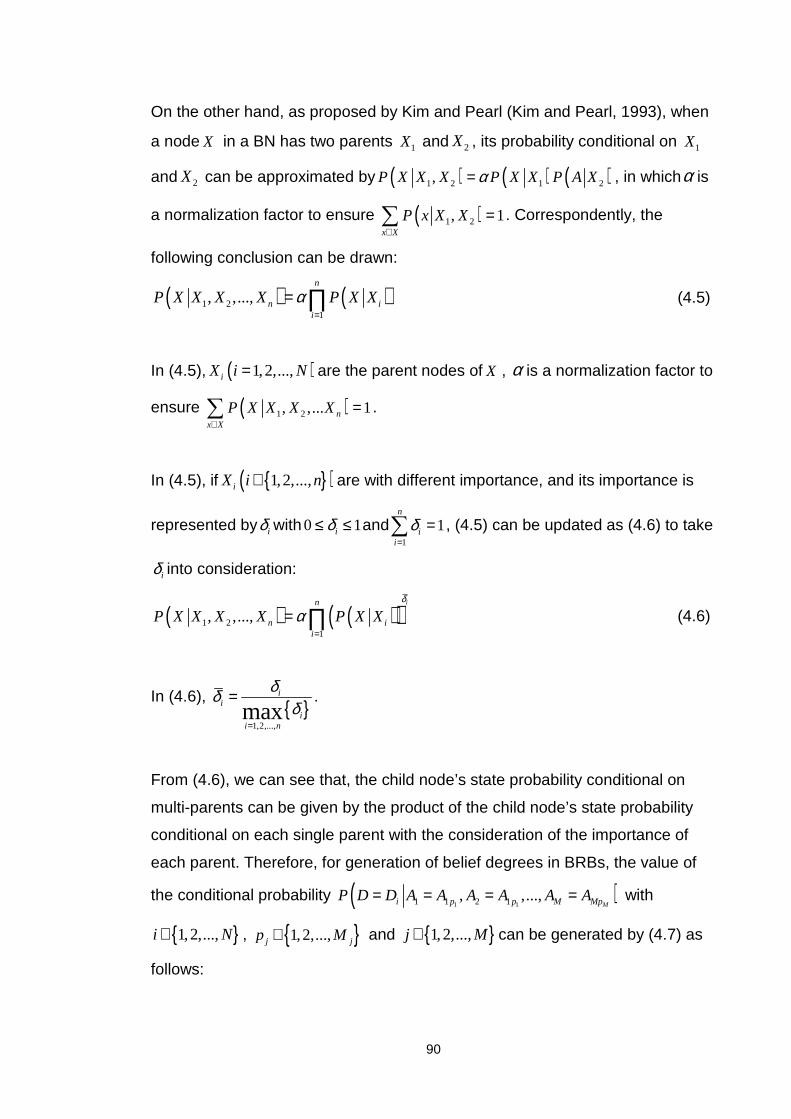
90
On the other hand, as proposed by Kim and Pearl (Kim and Pearl, 1993), when
a node X in a BN has two parents 1X and 2X , its probability conditional on 1X
and 2X can be approximated by ( ) ( ) ( )1 2 1 2,P X X X P X X P A Xα= , in whichα is
a normalization factor to ensure ( )1 2, 1x X
P x X X∈
=∑ . Correspondently, the
following conclusion can be drawn:
( ) ( )1 21
, ,...,n
n ii
P X X X X P X Xα=
= ∏ (4.5)
In (4.5), ( )1,2,...,iX i N= are the parent nodes of X , α is a normalization factor to
ensure ( )1 2, ,... 1nx X
P X X X X∈
=∑ .
In (4.5), if ( )1,2,...,iX i n∈ are with different importance, and its importance is
represented by iδ with0 1iδ≤ ≤ and1
1n
ii
δ=
=∑ , (4.5) can be updated as (4.6) to take
iδ into consideration:
( ) ( )( )1 21
, ,...,in
n ii
P X X X X P X Xδ
α=
= ∏ (4.6)
In (4.6),
1,2,...,max
ii
ii n
δδδ
=
= .
From (4.6), we can see that, the child node’s state probability conditional on
multi-parents can be given by the product of the child node’s state probability
conditional on each single parent with the consideration of the importance of
each parent. Therefore, for generation of belief degrees in BRBs, the value of
the conditional probability ( )1 11 1 2 1, ,...,Mi p p M MpP D D A A A A A A= = = = with
1,2,...,i N∈ , 1,2,...,j jp M∈ and 1,2,...,j M∈ can be generated by (4.7) as
follows:

91
( ) ( )( )1 11 1 2 11
, ,...,j
M j
M
i p p M Mp i j jpj
P D D A A A A A A P D D A Aδ
α=
= = = = = = =∏ (4.7)
In (4.7), 1,2,...,
maxj
j
jj n
δδ
δ=
= , in which jδ represents the importance of jA and
satisfies0 1jδ≤ ≤ and1
1n
jj
δ=
=∑ , α is a normalization factor to ensure
( )1 21 1 2 21
, ,..., 1M
N
i p p M Mpi
P D D A A A A A A=
= = = = =∑ .
Since the estimation of ( )ji j jpP D D A A= = with 1,2,...,i N∈ , 1,2,...,j M∈ and
1,2,...,j jp M∈ only needs the consideration of the state of one parent node at
a time, while the estimation of ( )1 11 1 2 1, ,...,Mi p p M MpP D D A A A A A A= = = = needs
simultaneous consideration of the state of M different parent nodes, to generate
( )1 11 1 2 1, ,...,Mi p p M MpP D D A A A A A A= = = = through the generation of
( )ji j jpP D D A A= = can significantly reduce bias and inconsistency involved in
the generation process.
Therefore, the generation of belief degrees in a BRB corresponding to Figure
4.1 is now dependent on the generation of each ( )ji j jpP D D A A= = for
1,2,...,i N= , 1,2,...,j M= and 1,2,...,j jp M= in a rational way.
Normally, ( )ji j jpP D D A A= = ( )1,2,...,i N= are specified by experts, using their
knowledge and experience. When the value of N is small, such a method may
be feasible. However, estimating ( )ji j jpP D D A A= = for all 1,2,...,i N= directly
needs the consideration of N different states at one time, thus, with the increase
of the value of N , direct estimation of ( )ji j jpP D D A A= = may inevitably involve
bias and inaccuracy.
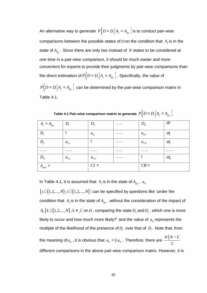
92
An alternative way to generate ( )ji j jpP D D A A= = is to conduct pair-wise
comparisons between the possible states of D on the condition that jA is in the
state ofjjpA . Since there are only two instead of N states to be considered at
one time in a pair-wise comparison, it should be much easier and more
convenient for experts to provide their judgments by pair-wise comparisons than
the direct estimation of ( )ji j jpP D D A A= = . Specifically, the value of
( )ji j jpP D D A A= = can be determined by the pair-wise comparison matrix in
Table 4.1.
Table 4.1 Pair-wise comparison matrix to generate ( )ji j jpP D D A A= =
jj jpA A= 1D 2D …… ND ω
1D 1 12a ……
1Na 1ω
2D 21a 1 …… 2Na 2ω
…… …… …… …… …… ……
ND 1Na 2Na …… 1 Nω
maxλ = CI = CR =
In Table 4.1, it is assumed that jA is in the state ofjjpA , sta
( )1,2,..., ; 1,2,...,s N t N∈ ∈ can be specified by questions like ‘under the
condition that jA is in the state ofjjpA , without the consideration of the impact of
( )1,2,..., ,kA k N k j∈ ≠ on D , comparing the state sD and tD , which one is more
likely to occur and how much more likely?’ and the value of sta represents the
multiple of the likelihood of the presence of sD over that of tD . Note that, from
the meaning of sta , it is obvious that 1ts sta a= . Therefore, there are ( )1
2
N N −
different comparisons in the above pair-wise comparison matrix. However, it is

93
sufficient to provide 1N − inter-related comparisons rather than all the( )1
2
N N −
different comparisons, although it is useful to have more comparisons for
consistency check.
Similar to Saaty’s AHP (Saaty, 1980), the relative priorities of sD can be
generated from the maximum eigenvector ( )1 2, ,...,T
Nω ω ω ω= of the matrix
( )st N Na
× in Table 4.1 and the consistency of the pair-comparison matrix can be
checked by the Consistency RatioCR CI RI= , whereCI is the Consistency
Index, which is defined by ( ) ( )max 1N Nλ − − with maxλ be the maximum eigen-
value corresponding toω ,and RI is a Random Index related to N as shown in
Table 4.2 (Tummala and Ling, 1998). Normally, a pair-wise comparison matrix
with CR less than 0.10 is considered acceptable.
Table 4.2 Random Index
n 1 2 3 4 5 6 7 8 9 10
RI 0 0 0.58 0.90 1.12 1.24 1.32 1.41 1.45 1.49
Since the sum of all the elements in ω is 1, and its ith element iω represents the
relative importance of the state iD among all the states from 1D to ND when jA
takes the value ofjjpA , iω can be interpreted as the conditional probability
( )ji j jpP D D A A= = , as represented in (4.6):
( )ji j jp iP D D A A ω= = = (4.8)
From (4.7), (4.8) and Table 4.1, ( )1 11 1 2 1, ,...,Mi p p M MpP D D A A A A A A= = = = can be
calculated, further, according to (4.4), the belief degrees in the BRB
corresponding to Figure 4.1 can be generated.
4.3 A brief introduction inference scheme of RIMER

94
Based on the generated BRBs, RIMER can be used to generate security
assessment result of a port storage area along a CLSC against cargo theft. In
this section, a brief introduction of the inference scheme of RIMER is provided.
Generally, the process of RIMER inference starts with the transformation of
input to BRBs, after which, the belief rules in BRBs relevant to the transformed
input are activated with different strengths, and the consequences of the
activated rules are then aggregated using the ER approach to generate the
inference result. Before the process of RIMER inference is introduced, the ER
approached is reviewed briefly.
4.3.1 The ER approach
In essence, the kennel of the ER approach is an algorithm to aggregate
information of different evidence to generate a synthesized view of the
evidence. Assume that there are L basic evidence, 1 2, ,..., Le e e , the information of
which is to be aggregated, and evidence ( )1,2,...,ie i L∈ can be described by
the following belief distribution:
( ) ( ) ( ) ( ) 1 1, 2 2, ,, , , ,..., ,i i i N N iS e H H Hβ β β= (4.9)
In (4.9), ( )1,2,...,nH n N= are the grades used to describe ie , and ,n iβ is the
degree to which ie can be described by nH . According to the definition of belief
distribution, in (4.9), if ,1
1N
n in
β=
=∑ , the information regarding ie is complete,
otherwise, if ,1
1N
n in
β=
<∑ , it is incomplete. In addition, for each ie , its importance is
represented by its weight, i.e., iω .
On the other hand, if evidence E is used to represent the aggregated view of ie
for all 1,2,...,i L= , (4.10) can then be used to represent E as follows:
( ) ( ) ( ) ( ) 1 1 2 2, , , ,..., ,N NS E H H Hβ β β=
(4.10)
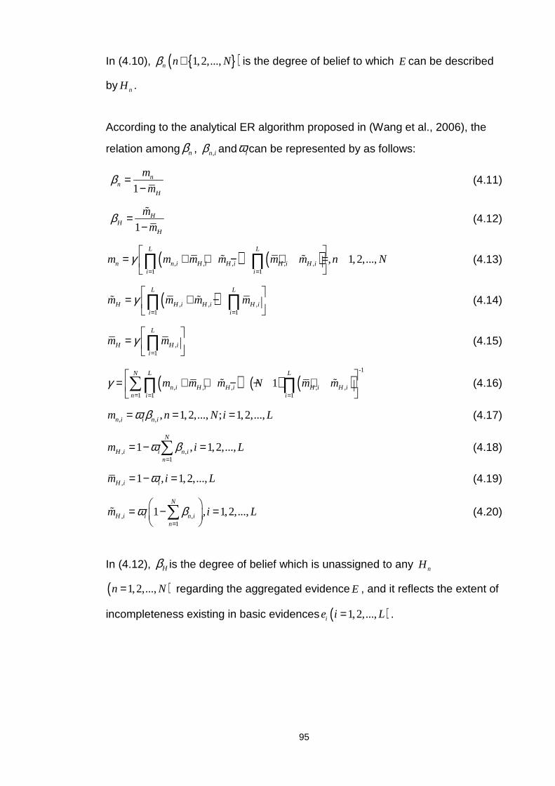
95
In (4.10), ( )1,2,...,n n Nβ ∈ is the degree of belief to which E can be described
by nH .
According to the analytical ER algorithm proposed in (Wang et al., 2006), the
relation among nβ , ,n iβ and iω can be represented by as follows:
1
nn
H
m
mβ =
− (4.11)
1
HH
H
m
mβ =
−ɶ
(4.12)
( ) ( ), , , , ,1 1
, 1,2,...,L L
n n i H i H i H i H ii i
m m m m m m n Nγ= =
= + + − + = ∏ ∏ɶ ɶ
(4.13)
( ), , ,1 1
L L
H H i H i H ii i
m m m mγ= =
= + − ∏ ∏ɶ ɶ (4.14)
,1
L
H H ii
m mγ=
= ∏ (4.15)
( ) ( ) ( )-1
, , , , ,1 1 1
1L LN
n i H i H i H i H in i i
m m m N m mγ= = =
= + + − − + ∑∏ ∏ɶ ɶ (4.16)
, , , 1,2,..., ; 1,2,...,n i i n im n N i Lω β= = = (4.17)
, ,1
1 , 1,2,...,N
H i i n in
m i Lω β=
= − =∑ (4.18)
, 1 , 1,2,...,H i im i Lω= − = (4.19)
, ,1
1 , 1,2,...,N
H i i n in
m i Lω β=
= − = ∑ɶ (4.20)
In (4.12), Hβ is the degree of belief which is unassigned to any nH
( )1,2,...,n N= regarding the aggregated evidence E , and it reflects the extent of
incompleteness existing in basic evidences ( )1,2,...,ie i L= .

96
Based on the value of ( )1,2,...,n n Nβ = and Hβ , the utility of the aggregated
result regarding E in (4.10) can be calculated through (4.21) and (4.22) as
follows with the assumption that 1nH + is preferable to nH :
( ) ( )1 1min2
N
H i ii
U E U Uβ β β=
= + +∑ (4.21)
( ) ( )1
max1
N
i i N H Ni
U E U Uβ β β−
=
= + +∑
(4.22)
In (4.21) and (4.22), ( )1,2,...,iU i N= is the utility of iH in (4.10). It can be seen
that the utility of E is represented by an interval due to the impact of Hβ , and the
lower and upper bound of the interval are calculated by (4.21) and (4.22),
respectively. In addition, the average of the lower and upper bound of the
interval defined by (4.21) and (4.22) is usually considered as the representative
utility of the aggregated evidence E in (4.10), and it can be calculated as:
( ) ( ) ( ) ( )min max1
1
1
2 2
N
n n N Hrepn
U E U EU E U U Uβ β
=
+= = + +∑ (4.23)
Note that, if the information regarding ie is complete for all 1,2,...,i L= , 0Hβ =
and ( ) ( ) ( )min max1
N
i irepi
U E U E U E Uβ=
= = =∑ .
4.3.2 Input information
For the convenience of discussion, it is assumed that in a BRB, there are M
antecedents, represented by: 1 2, ,..., MA A A , and the consequence of the BRB is
represented by D , further, the kth rule of the BRB is represented by (4.2).
Due to the complexity of many practical problems, the input information to the
BRB, i.e., the information about 1 2, ,..., MA A A , is always represented in different
forms, e.g., quantitative, qualitative, categorized, fuzzy, etc. By using the
transformation methods proposed by Yang (2001), the information regarding

97
every antecedent can be represented by a belief distribution, e.g., the
information regarding antecedent iA can be represented by:
( ) ( ) ( ) ( ) 1 1 2 2, , , ,... ,i ii i i i i iM iMS A A A Aα α α=
(4.24)
In (4.24), ( )1,2,..., ; 1,2,...,ij iA i M j M∈ = are the referential values which can be
taken by iA or the grades used to describe iA , while ijα is the degree to which iA
can take the value of ijA or can be described by the grade of ijA .
4.3.3 Rule activation
After the input information regarding all ( )1,2,...,iA i M= is transformed into the
form of (4.24), the input corresponding to the kth rule in the BRB as represented
by (4.2) can be denoted as:
( ) ( ) ( )1 1 2 21 1 2 2, , ... ,
M M
k k k k k kp p p p Mp MpA A Aα α α∧ ∧ ∧ (4.25)
In (4.25), , 1,2,..., , , 1,2,...,i i
k kip ij i ip ij iA A j M j Mα α∈ = ∈ = , and the total match
degree of the input and the packet antecedent in the kth rule, kα , can be
calculated by (4.26) as:
( )1
ki
i
Mk
k ipi
δα α
=
= ∏
(4.26)
In (4.26), kiδ satisfies (4.27) as follows:
1,2,...,
maxki
kiki
i M
δδδ
=
= (4.27)
According to kα in (4.26), the activation weight of the kth rule, kω , which
indicates the strength of the activation of the kth rule, can be specified by (4.28)
as follows by incorporating the weight of the kth rule kθ :
1
k kk L
i ii
θ αωθ α
=
=∑
(4.28)
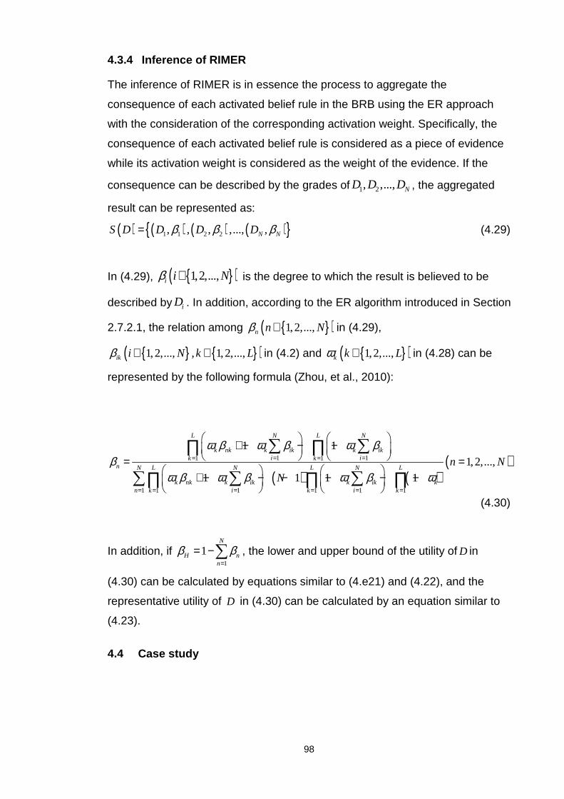
98
4.3.4 Inference of RIMER
The inference of RIMER is in essence the process to aggregate the
consequence of each activated belief rule in the BRB using the ER approach
with the consideration of the corresponding activation weight. Specifically, the
consequence of each activated belief rule is considered as a piece of evidence
while its activation weight is considered as the weight of the evidence. If the
consequence can be described by the grades of 1 2, ,..., ND D D , the aggregated
result can be represented as:
( ) ( ) ( ) ( ) 1 1 2 2, , , ,..., ,N NS D D D Dβ β β= (4.29)
In (4.29), ( )1,2,...,i i Nβ ∈ is the degree to which the result is believed to be
described by iD . In addition, according to the ER algorithm introduced in Section
2.7.2.1, the relation among ( )1,2,...,n n Nβ ∈ in (4.29),
( )1,2,..., , 1,2,...,ik i N k Lβ ∈ ∈ in (4.2) and ( )1,2,...,k k Lω ∈ in (4.28) can be
represented by the following formula (Zhou, et al., 2010):
( ) ( )( )1 11 1
1 1 11 1 1
1 1
1,2,...,
1 1 1 1
L LN N
k nk k ik k iki ik k
n L L LN N N
k nk k ik k ik kn i ik k k
n N
N
ω β ω β ω ββ
ω β ω β ω β ω
= == =
= = == = =
+ − − − = =
+ − − − − − −
∑ ∑∏ ∏
∑ ∑ ∑∏ ∏ ∏ (4.30)
In addition, if 1
1N
H nn
β β=
= −∑ , the lower and upper bound of the utility of D in
(4.30) can be calculated by equations similar to (4.e21) and (4.22), and the
representative utility of D in (4.30) can be calculated by an equation similar to
(4.23).
4.4 Case study

99
4.4.1 Generation of belief degrees in BRBs in the s ecurity assessment model in Appendix 1
In the security assessment model in Appendix 1, there are totally 36 BRBs
involved, and each BRB is corresponding to a basic BN fragment, which can be
represented by Figure 4.1. To demonstrate the applicability of the process and
method proposed in this chapter, the BRB regarding the relation among Lighting
Coverage (LCO), Lighting Capability (LCA) and the performance of Lighting
Facility (LF) is generated as follows.
According to Appendix 2 and Appendix 3, in the BRB, LCO can take three
referential values, i.e., ‘Wide’ (W), ‘Moderate’ (M) and ‘Limited’ (L), LCA can
take three referential values, namely, ‘High’ (H), ‘Moderate’ (M) and ‘Low’ (L),
and ‘Good’ (G), ‘Moderate’ (M) and ‘Poor’ (P) are the referential values taken by
LF. To generate the belief degrees to which LF can take the referential values
of G, M and P according to the combination of referential values taken by LCO
and LCA, the conditional probability ( ),P LF LCO LCA should be specified
according to the relation between BRB and BN as discussed previously.
Specifically, the conditional probability ( )P LF LCO and ( )P LF LCA should be
generated respectively to generate ( ),P LF LCO LCA .
From the perspective of BN, when the state of LCA is M, the experts, e.g., the
PFSOs of different ports along CLSCs, should fill out the following pair-wise
comparison matrix in Table 4.3 by answering questions like ‘neglecting the
influence of LCO on LF, when LCA is in the state of M, which state of LF is
more likely to occur, and how much more likely?’ For instance, in the pair-wise
comparison matrix represented by Table 4.3 as follows, given that LCA is in the
state of M, the possibility of LF being M is 5 times as the possibility of LF being
G, and the possibility of LF being P is the same as the possibility of LF being H.
This is reasonable since if the capability of lighting system is judged to be
‘Moderate’, it is likely that the performance of the system is also ‘Moderate’, and
the chances that it may be ‘Good’ or ‘Poor’ may be more or less the same. .

100
Table 4.3 Pair-wise comparison matrix to generate ( )P LF LCA when LCA M=
LCA=M G M P ω
G 1 1/5b 1b 0.1429Gω =
M 5a 1 5b 0.7142Mω =
P 1a 1/5a 1 0.1429Lω =
0CR = 0CI = max 3λ =
a: Experts’ judgments b: Reciprocal of the expert’s judgments
From Table 4.3, the following results can be generated according to the
discussion in Section 4.2.3:
( ) 0.1429P LF G LCA M= = =
( ) 0.7142P LF M LCA M= = =
( ) 0.1429P LF P LCA M= = =
Similarly, we can get the probability of states of LF on the condition that the
state of LCA is H and L, and the results can be summarized in Table 4.4 as
follows:
Table 4.4 The probabilities of LF conditional on LC A’s different states
LF LCA=H LCA=M LCA=L
G 0.7153 0.1429 0.0823
M 0.1870 0.7142 0.3150
P 0.0977 0.1429 0.6027
In the same way, the probabilities of the states of LF conditional on different
states of LCO are listed in Table 4.5.
Table 4.5 The probabilities of LF conditional on LC O’s different states
LF LCO=W LCO=M LCO=L
G 0.7608 0.0909 0.0660
M 0.1576 0.8182 0.3187
P 0.0816 0.0909 0.6153
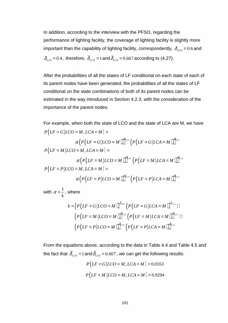
101
In addition, according to the interview with the PFSO, regarding the
performance of lighting facility, the coverage of lighting facility is slightly more
important than the capability of lighting facility, correspondently, 0.6LCOδ = and
0.4LCAδ = , therefore, 1LCOδ = and 0.667LCAδ = according to (4.27).
After the probabilities of all the states of LF conditional on each state of each of
its parent nodes have been generated, the probabilities of all the states of LF
conditional on the state combinations of both of its parent nodes can be
estimated in the way introduced in Section 4.2.3, with the consideration of the
importance of the parent nodes.
For example, when both the state of LCO and the state of LCA are M, we have
( )( )( ) ( )( ),
LCO LCA
P LF G LCO M LCA M
P LF G LCO M P LF G LCA Mδ δ
α
= = = =
= = = =
( )( )( ) ( )( ),
LCO LCA
P LF M LCO M LCA M
P LF M LCO M P LF M LCA Mδ δ
α
= = = =
= = = =
( )( )( ) ( )( )
,
LCO LCA
P LF P LCO M LCA M
P LF P LCO M P LF P LCA Mδ δ
α
= = = =
= = = =
with 1
kα = , where
( )( ) ( )( )( )( ) ( )( )( )( ) ( )( )
LCO LCA
LCO LCA
LCO LCA
k P LF G LCO M P LF G LCA M
P LF M LCO M P LF M LCA M
P LF P LCO M P LF P LCA M
δ δ
δ δ
δ δ
= = = = = +
= = = = +
= = = =
From the equations above, according to the data in Table 4.4 and Table 4.5 and
the fact that 1LCOδ = and 0.667LCAδ = , we can get the following results:
( ), 0.0353P LF G LCO M LCA M= = = =
( ), 0.9294P LF M LCO M LCA M= = = =
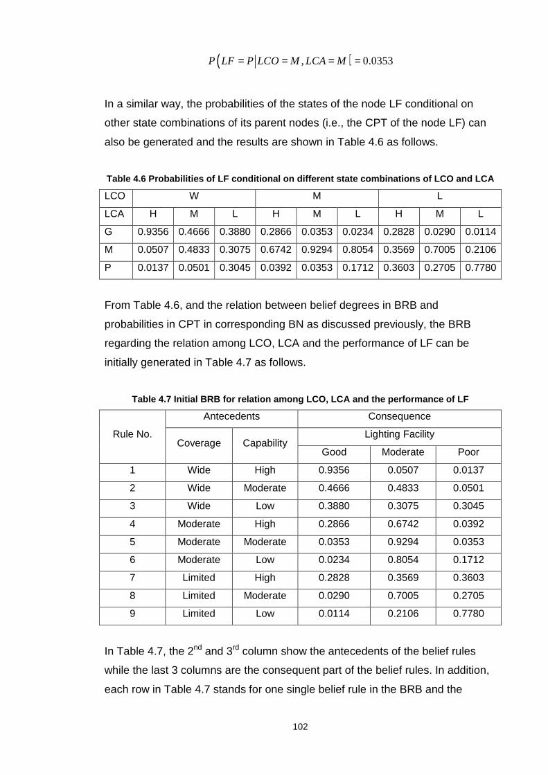
102
( ), 0.0353P LF P LCO M LCA M= = = =
In a similar way, the probabilities of the states of the node LF conditional on
other state combinations of its parent nodes (i.e., the CPT of the node LF) can
also be generated and the results are shown in Table 4.6 as follows.
Table 4.6 Probabilities of LF conditional on differ ent state combinations of LCO and LCA
LCO W M L
LCA H M L H M L H M L
G 0.9356 0.4666 0.3880 0.2866 0.0353 0.0234 0.2828 0.0290 0.0114
M 0.0507 0.4833 0.3075 0.6742 0.9294 0.8054 0.3569 0.7005 0.2106
P 0.0137 0.0501 0.3045 0.0392 0.0353 0.1712 0.3603 0.2705 0.7780
From Table 4.6, and the relation between belief degrees in BRB and
probabilities in CPT in corresponding BN as discussed previously, the BRB
regarding the relation among LCO, LCA and the performance of LF can be
initially generated in Table 4.7 as follows.
Table 4.7 Initial BRB for relation among LCO, LCA a nd the performance of LF
Rule No.
Antecedents Consequence
Coverage Capability Lighting Facility
Good Moderate Poor
1 Wide High 0.9356 0.0507 0.0137
2 Wide Moderate 0.4666 0.4833 0.0501
3 Wide Low 0.3880 0.3075 0.3045
4 Moderate High 0.2866 0.6742 0.0392
5 Moderate Moderate 0.0353 0.9294 0.0353
6 Moderate Low 0.0234 0.8054 0.1712
7 Limited High 0.2828 0.3569 0.3603
8 Limited Moderate 0.0290 0.7005 0.2705
9 Limited Low 0.0114 0.2106 0.7780
In Table 4.7, the 2nd and 3rd column show the antecedents of the belief rules
while the last 3 columns are the consequent part of the belief rules. In addition,
each row in Table 4.7 stands for one single belief rule in the BRB and the

103
numeric values in the last 3 columns stand for the belief degrees assigned to
the corresponding grades in the belief rules. For example, the row with the Rule
No. 2 in the table represents the following belief rule:
IF Coverage is Wide AND Capability is Moderate, the performance of Lighting
System is (Good, 0.4666), (Moderate, 0.4833), (Poor, 0.0501)
Note that although all belief degrees can be generated through CPT of the
corresponding BN, not all belief degrees can reasonably reflect the relation
among the factors involved. For example, if Coverage is ‘Wide’ and Capability is
‘High’, from the PFSO’s opinion, the performance of Lighting System should be
‘Good’ with the degree of 1, however, in the 1st belief rule in Table 4.7, the belief
degree assigned to ‘Good’ is 0.9356. A similar conclusion can be drawn
regarding the last belief rule in Table 4.7. Therefore, after the belief degrees are
generated through the generation of CPT of the corresponding BN, some belief
degrees may need to be revised according to experts’ knowledge regarding the
relation among the factors involved in the BRB. As for the BRB represented by
Table 4.7, after the revise of belief degrees, the BRB can be represented by
Table 4.8 as follows:
Table 4.8 Revised BRB for relation among LCO, LCA a nd the performance of LF
Rule No.
Antecedents Consequence
Coverage Capability Lighting Facility
Good Moderate Poor
1 Wide High 1.0000 0.0000 0.0000
2 Wide Moderate 0.4666 0.4833 0.0501
3 Wide Low 0.3880 0.3075 0.3045
4 Moderate High 0.2866 0.6742 0.0392
5 Moderate Moderate 0.0353 0.9294 0.0353
6 Moderate Low 0.0234 0.8054 0.1712
7 Limited High 0.2828 0.3569 0.3603
8 Limited Moderate 0.0290 0.7005 0.2705
9 Limited Low 0.0000 0.0000 1.0000
104
In a BRB, besides belief degrees, there are other parameters, i.e., rule weights
and antecedent weights, which also need to be specified. For the BRB in Table
4.8, according to the previous discussion, the antecedent weights of Coverage
and Capability are 0.6 and 0.4 respectively. Moreover, the weight of each belief
rule is initially set to be equal as there is no initial evidence to suggest that the
importance of the rules in the BRB should be different.
In the same way, the belief degrees of other 35 BRBs in the security
assessment model in Appendix 1 can be generated, and all the belief degrees
in the BRBs are listed in Appendix 5. In addition, similar to the BRB represented
by Table 4.8, all rule weights are set to be equal initially. As for antecedent
weights, they are specified according to subjective opinions of different PFSOs
and the characteristics and environment of different ports. Note that, for the
same antecedent, it may have different weights under the context of different
ports, which will be further explained in Section 4.3.2.
Due to the characteristics of CLSC operation, the initial specification of
parameters in all BRBs is highly dependent on the subjective judgments of
different experts. Therefore, it is essential to reduce bias and subjectivity
involved in the experts’ judgments to improve the reliability of inference results
based on BRBs. If there are real data available, the parameters can be trained
and updated using the training method (Yang, et al., 2007) as introduced in
Chapter 2 to increase the objectivity of the parameter values in BRBs. However,
if there is no data available, or if the available data is not enough to conduct
valid training, as is often the case for security assessment in CLSC, the process
proposed in this chapter will be important to ensure that experts’ judgments can
be provided in a consistent and robust manner.
4.4.2 Assessment of security level of port storage areas along CLSCs against cargo theft
After BRBs for the security assessment model in Appendix 1 are generated as
discussed above, the data collected from 5 different ports in both the UK and
China are used to assess the security level of the ports against cargo theft.

105
Specifically, the assessment using the data collected from a port in China, as
introduced in the case study in Section 3.4, is introduced in detail in this section.
In Section 3.4, the information collected from the port is measured by belief
distributions, according to which the assessment can be conducted in a bottom-
up way in the security assessment model in Appendix 1. For example,
according to the PFSO’s response to the questionnaire, the lighting facility
illuminates all entrances/exits and all loading/unloading areas of the port and
vehicles/individuals are identifiable in most cases under the lighting area
through CCTV. According to the meanings of the grades/referential values listed
in Appendix 2, the Coverage of lighting facility can be represented as: (Wide,
1), (Moderate, 0), (Limited, 0) while the Capability of lighting facility can be
represented as (High, 0), (Moderate, 1) (Low, 0). Based on the BRB in Table
4.8 and the relevant antecedent weights and rule weights, the performance of
Lighting Facility can be generated by the application of RIMER as:
(Good, 0.4666), (Moderate, 0.4833), (Poor, 0.0501)
Similarly, according to the information of basic factors regarding CCTV Facility,
its performance is
(Good, 0.1712), (Moderate, 0.8054), (Poor, 0.0234)
Therefore, the performance of Monitor Facility is
(Good, 0.1976), (Moderate, 0.7670), (Poor, 0.0354)
In the same way, the performance of Control Facility is given by
(Good, 0.6954), (Moderate, 0.2328), (Poor, 0.0719)
Thus, the performance of Hardware Facility can be generated as
(Good, 0.3330), (Moderate, 0.6184), (Poor, 0.0485)
As the performance of Software Facility is given by
(Good, 1), (Poor, 0)
the Facility Feature can be represented as
(Good, 0.4710), (Moderate, 0.4937), (Poor, 0.0353)
Further, due to the fact that the Historical Feature and Employee Feature of the
port can be represented by
(Good, 0), (Moderate, 1), (Poor, 0)
and
(Good, 1), (Poor, 0)

106
the Physical Feature of the port can be generated as
(Good, 0.6761), (Moderate, 0.2895), (Poor, 0.0344)
Thus, the Vulnerability of the port is
(Vulnerable, 0.0867), (Medium, 0.5031), (Not Vulnerable, 0.4102)
because the Intervention Measures can be generated as
(Effective, 0.6894), (Moderate, 0.2039), (Not Effective, 0.1068)
according to information on relevant basic factors. On the other hand, the
Threat Likelihood and Potential Consequence regarding cargo theft in the port
can be generated as
(Quite Likely, 0.0055), (Likely, 0.0501), (Not Likely, 0.0479), (Impossible,
0.7271), (Unknown, 0.1693)
and
(Catastrophic, 0.0274), (Severe, 0.0634), (Moderate, 0.1106), (Not
Severe, 0.0973), (None, 0.3697), (Unknown, 0.3316)
Therefore, the Overall Security of the port against cargo theft is
(Very High, 0.7122), (High, 0.0382), (Moderate, 0.0754), (Low, 0.0256),
(Very Low, 0.0242), (Unknown, 0.1245) (4.31)
The information contained in the belief distribution in (4.31) can be explained as
follows: A large portion of the basic factors in the model makes the overall
security level be ‘Very High’, as reflected by the belief degree of 0.7122
assigned to the grade of ‘Very High’. Although the security level of the port
against theft is very high in general, there are still some aspects which require
attention, as there is 0.0256 of belief degree assigned to ‘Low’ and even 0.0242
assigned to ‘Very Low’. Another point which needs attention is that there is a
certain degree (0.1245) assigned to ‘Unknown’, which means that there is no
information available in the port for some basic factors in the security
assessment model. In summary, the result represented by the belief distribution
in (4.31) indicates that the security level of the storage area in the port against
cargo theft is ‘Very High’ in general, but there are still a few areas that need to
be improved. Further analysis is needed to reveal which specific areas need
improvement and how to improve it in an optimal way. In addition, to reduce the

107
extent of incompleteness in the security assessment result, more information
needs to be collected.
Furthermore, in order to generate an overall view of the security level, the idea
of utility can be used. If the utilities of ‘Very High’, ‘High’, ‘Medium’, ‘Low’ and
‘Very Low’ are 1, 0.75, 0.5, 0.25 and 0 respectively, the utility interval of the
overall security level can be calculated by (4.21) and (4.22), and the result is
[0.7849, 0.9094], while the representative utility, which can be calculated by
(4.23), is 0.8472. Such a utility also indicates that the overall security level
against cargo theft in the port is very good in general. On the other hand, in the
questionnaire, the PFSO also gave an overall score of 0.8 to indicate the overall
security level against cargo theft in the port according to his own impression. It
can be seen that the result generated by the security assessment model
proposed in the thesis is not far from the judgment provided by the PFSO.
However, although it is convenient for comparison, to represent security level
with a single utility or a single score can only reveal the average performance
but not the diverse nature of people’s perception, which can be represented by
belief distributions, as discussed previously. In addition, from the average utility
of 0.8472, it cannot be revealed that there are some factors in the port which
lead to ‘Very Low’ security level, which, on the other hand, can be reflected by
belief distributions in (4.31) conveniently.
Apart from the validation using the data collected in the above port, the model
developed in the thesis is also validated using the data collected from four other
ports in the UK and China. The assessment results generated using the data for
each port as well as the personal judgments by the PFSO of each port are
summarized in Table 4.9 in next page.
In Table 4.9, the ports selected for validation are numbered from 1 to 5; the
terms ‘V.H.’, ‘H.’, ‘M.’, ‘L.’, ‘V.L.’ and ‘U.’ stand for the grades of ‘Very High’,
‘High’, ‘Medium’, ‘Low’, ‘Very Low’ and ‘Unknown’ respectively; ‘Rep.’ stands for
‘Representative value’ of the utility. In addition, the judgment of PFSO are
expressed as ‘Score from PFSO’ and the score is either given directly by the
PFSO or transformed from a belief distribution provided by the PFSO describing

108
the security level of the corresponding port against cargo theft. In the last
column, the relative error between the result generated by the model and the
corresponding judgment of PFSO is represented in percentage terms.
Table 4.9 Security Assessment Results for different ports in the UK and China
N
o.
Belief degrees generated by the model Utility Score
from
PFSO
Error V.H. H. M. L. V.L. U. Interval Rep.
1 0.375 0.057 0.138 0.049 0.039 0.343 [0.499, 0.842] 0.670 0.66 1.51%
2 0.712 0.038 0.075 0.026 0.024 0.124 [0.785, 0.909] 0.847 0.8 5.88%
3 0.377 0.058 0.131 0.047 0.038 0.349 [0.498, 0.846] 0.672 0.66 1.82%
4 0.554 0.143 0.210 0.050 0.044 0 0.778 0.778 0.7 11.14%
5 0.616 0.078 0.204 0.058 0.043 0 0.791 0.791 0.75 5.47%
Note that for different ports the weight of the same factor may be different. For
example, to evaluate the Security Level, the following 3 factors are considered:
Threat Likelihood (TL), Vulnerability (VUL) and Potential Consequence (PC).
For a certain port, since there are critical infrastructures around the port, severe
consequence is not affordable. Thus the weight of PC should be high. However,
for another port, since it is far from city centre, and according to the PFSO’s
opinion, VUL is the most controllable factors among TL, VUL and PC, so, VUL
should have the largest weight. The results in Table 4.9 are generated based on
port-specific set of parameters in the security assessment model in Appendix 1
Due to the sensitivity of the information or the complexity of CLSC security
assessment, some information regarding basic factors in the security
assessment model could not be collected through questionnaires or interviews
for Port 1, Port 2 and Port 3, resulting in incomplete assessment results of the 3
ports. The incompleteness is explicitly modelled by the non-zero degree
assigned to the grade of ‘Unknown’ or the whole set of the assessment grades.
Correspondently, the utilities of the assessment results for Port 1, Port 2 and
Port 3 are intervals instead of precise values, and from Table 4.9, it can be seen
that the width of utility interval increases with the degree assigned to the grade
of ‘Unknown’. For the convenience of comparison, the average of the lower and
upper bounds of the interval is taken as a representative value of the interval.

109
From Table 4.9, we can see that according to the input information, i.e., the
information regarding basic factors in the security assessment model, and the
initial parameters of the BRBs, the results generated by the security
assessment model proposed in the thesis and the judgments provided by the
PFSOs are close to each other, indicating that the model developed in the
thesis is valid and practical.
Note that in the above case studies the security level of a port along a CLSC
against cargo theft is assessed. In a similar way, the security level of a port
along a CLSC against other threats can also be assessed, and thus the security
level of a port along a CLSC can be assessed. Also, the security of other
organizations involved in a CSLC can be assessed in the same way. Further,
based on the security level of each organization in a CLSC, the security level of
a whole CSLC can be generated after the relationships among the
organizations are identified, analyzed and modelled properly.
4.5 Conclusion
Due to its capability to accommodate and handle different forms of information
with different kinds of uncertainty, RIMER is selected as a tool to conduct
security assessment in CLSC. To generate belief degrees in BRBs for the
security assessment model, which is the basis for the application of RIMER, a
new process is proposed in this chapter. The most important feature of the
process is that it can significantly reduce the bias and inconsistency in experts’
judgments when belief degrees in the BRBs are generated. This character is
especially useful when there is insufficient real data available for parameter
training to reduce bias and subjectivity involved in the specification of the
parameters. Further, according to the generated BRBs and the data collected
from different ports in both China and the UK, the security level of each port
against cargo theft is assessed, and the comparison between the security
assessment results generated by the model and the security assessment
results given by corresponding PFSOs according to their experience and
judgments reveals that the model developed in the thesis is practical and valid
110
for security assessment under the context of CLSC. Moreover, in a similar way,
the model can also be applied to assess the security of ports against other
threats besides cargo theft, the security of other organizations involved in a
CLSC, and the security of a whole CLSC, with the relationship among the
organizations in the CLSC identified, analyzed and modelled properly.
The discussion in this chapter and the discussion in Chapter 3 constitute the
basis of security analysis, .i.e., security assessment, under the context of
CLSC. According to the discussion in the two chapters, to assess security of a
whole CLSC, the CLSC should be firstly divided into different stages according
to a typical voyage of a container along a CLSC, and the security assessment
of a certain stage against a certain threat faced by the stage is considered as a
basic unit for security assessment of the whole CLSC. Due to the advantages of
RIMER as discussed in Chapter 2, it is selected as a method to conduct
security assessment of a basic unit, and the security assessment result of each
basic unit regarding a CLSC is then aggregated to form the security level of the
whole CLSC with the application of RIMER by considering the interactions
among different basic units.
Based on the security level generated, the next step is to develop responsive
measures to improve the security level in an optimal way, which is the topic of
the next chapter.

111
5 Chapter 5 Assessment based resource allocation to i mprove security in CLSC
Abstract
The ultimate aim of security analysis in this thesis from a practical point of view
is to provide assistance for industrial practitioners in ensuring the secure
operation of CLSC. If security level is assessed to be not satisfactory,
responsive measures are needed for security improvement. Since resources for
security improvement are always limited, in this chapter, under the framework of
RIMER, a set of new models are developed to optimally allocate limited
resources to improve CLSC security based on security assessment results, so
that resources can be used in an efficient and effective way. The proposed
models are then validated using a case study about the improvement of the
performance of an access control system in a port to prevent cargo theft.
5.1 Introduction
Similar to risk management, which is a process of identifying risk, assessing risk,
and taking steps to reduce risk to an acceptable level (Stoneburner et al., 2002),
security analysis also contains the phases of threat identification, security level
assessment as well as development of responsive measures to improve the
security to a certain level based on security assessment result. In Chapter 3
and Chapter 4, possible threats faced by CLSC operation are identified, and the
security level for CLSC can be assessed by applying RIMER based on the
security assessment model developed. As for the development of responsive
measures to improve CLSC security, since the resources for security
improvement (e.g. budget, man power, etc.) are always limited, it is necessary
to optimally allocate the limited resources based on the security assessment
result, so that the security can be improved to a satisfactory level by consuming
minimal resources or the available resources can be used in an efficient way to
generate maximum security improvement. Facing this situation, this chapter
intends to propose a method to assist security improvement by optimally
allocating resources based on security assessment result under the context of
CLSC.

112
5.2 Sensitivity analysis of RIMER
As discussed in Chapter 2, due to the advantages of RIMER over other existing
methods for resource allocation in response to security and safety incidents, it is
selected as a basis for the development of security based resource allocation
model for CLSC security improvement.
To find out how to allocate limited resources efficiently and effectively among
basic factors to improve security level according to security assessment result
generated by RIMER, it is necessary to investigate how influential each basic
factor is towards the security level, therefore, a sensitivity analysis under the
framework of RIMER is conducted in this section.
5.2.1 Basis of sensitivity analysis
The process of the sensitivity analysis is demonstrated on the basis of Figure
4.1, in which, there are 2 levels of factors: factor D at the top level is considered
as the security level or security-related performance while the factor
1 2, ,..., MA A A at the bottom level are considered as basic factors which can
influence the security level or security-related performance D . Note that, such a
2-level model is just a simplification of reality, and the method for sensitivity
analysis in such a simplified model can be generalized to a security assessment
model with multiple levels for real problems.
In Figure 4.1, ( )1,2,...,iA i M= can take iM referential values 1 2, ,ii i iMA A A and the
degree to which iA can take the value of ijA is represented by
( )1,2,..., ; 1,2,...,ij ii M j Mα = = with [ ]0,1ijα ∈ and1
1iM
ijj
α=
≤∑ . Correspondently, the
information regarding iA can be represented by a belief distribution in (4.24),
and IiU , the representative utility of iA , can be calculated by (5.1) as follows with
IijU being the utility of ijA and [ ]0,1I
ijU ∈ :
( )11 1
11
2
i i
i
M MI I I Ii ij ij i iM ij
j j
U U U Uα α= =
= + + −
∑ ∑ (5.1)
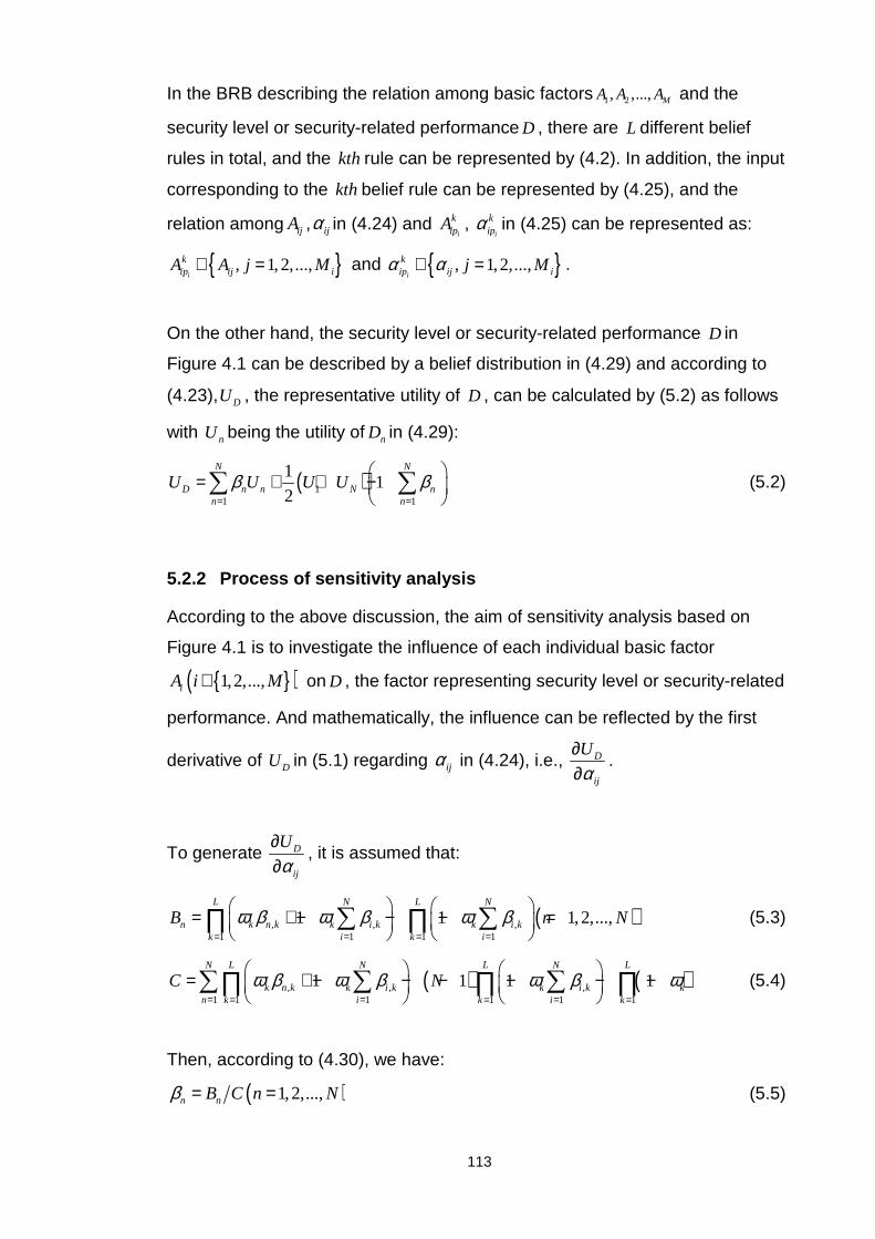
113
In the BRB describing the relation among basic factors 1 2, ,..., MA A A and the
security level or security-related performance D , there are L different belief
rules in total, and the kth rule can be represented by (4.2). In addition, the input
corresponding to the kth belief rule can be represented by (4.25), and the
relation among ijA , ijα in (4.24) and i
kipA ,
i
kipα in (4.25) can be represented as:
, 1,2,...,i
kip ij iA A j M∈ = and , 1,2,...,
i
kip ij ij Mα α∈ = .
On the other hand, the security level or security-related performance D in
Figure 4.1 can be described by a belief distribution in (4.29) and according to
(4.23), DU , the representative utility of D , can be calculated by (5.2) as follows
with nU being the utility of nD in (4.29):
( )11 1
11
2
N N
D n n N nn n
U U U Uβ β= =
= + + −
∑ ∑ (5.2)
5.2.2 Process of sensitivity analysis
According to the above discussion, the aim of sensitivity analysis based on
Figure 4.1 is to investigate the influence of each individual basic factor
( )1,2,...,iA i M∈ on D , the factor representing security level or security-related
performance. And mathematically, the influence can be reflected by the first
derivative of DU in (5.1) regarding ijα in (4.24), i.e., D
ij
U
α∂∂
.
To generate D
ij
U
α∂∂
, it is assumed that:
( ), , ,1 11 1
1 1 1,2,...,L LN N
n k n k k i k k i ki ik k
B n Nω β ω β ω β= == =
= + − − − =
∑ ∑∏ ∏ (5.3)
( ) ( ), , ,1 1 11 1 1
1 1 1 1L L LN N N
k n k k i k k i k kn i ik k k
C Nω β ω β ω β ω= = == = =
= + − − − − − −
∑ ∑ ∑∏ ∏ ∏ (5.4)
Then, according to (4.30), we have:
( )1,2,...,n nB C n Nβ = = (5.5)

114
Further, we define:
( ) ( ),11,
1 1,2,...,L N
k i kik k q
q q Lξ ω β== ≠
− =
∑∏≜ (5.6)
( ) ( ), ,11,
, 1 1,2,..., ; 1,2,...L N
k j k k i kik k q
q j q L j Nχ ω β ω β== ≠
+ − = =
∑∏≜ (5.7)
Therefore, from (5.3) to (5.7), we have:
2
1n nn
k k k
B CC B
C
βω ω ω
∂ ∂ ∂= ⋅ − ⋅ ∂ ∂ ∂ (5.8)
( ) ( ), , ,1 1
,N N
nn k i k i k
i ik
Bk n kβ β χ ξ β
ω = =
∂ = − + ∂ ∑ ∑ (5.9)
( ) ( ) ( ) ( ), , ,1 1 1 1,
, 1 1 LN N N
j k i k i k qj i i q q kk
Ck j N kβ β χ ξ β ω
ω = = = = ≠
∂ = − + − + − ∂ ∑ ∑ ∑ ∏ (5.10)
On the other hand, according to reasoning process of RIMER as introduced in
Chapter 2, we have:
, , ,
i
i
qipqn kD D
qn k q iij n k q ip ij
U U ααβ ωα β ω α α α
∂∂∂ ∂∂ ∂= ⋅ ⋅ ⋅ ⋅∂ ∂ ∂ ∂ ∂ ∂∑ (5.11)
In (5.11), each component can be calculated as follows:
According to (5.2),
( )11
1
11
2
1
N
n N nnD
Nn
n nn
U U UU
U
β
β β
=
=
− + <∂ = ∂ =
∑
∑ (5.12)
n
k
βω
∂∂
can be generated through (5.8)-(5.10).
According to (4.26) to (4.28), we can get:
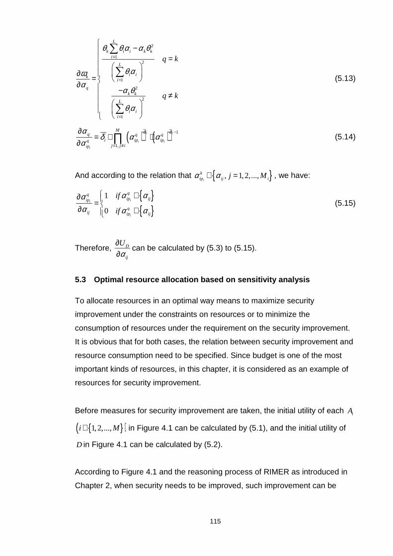
115
2
12
1
2
2
1
L
k i i k ki
L
i iki
qk k
L
i ii
q k
q k
θ θ α α θ
θ αωα
α θ
θ α
=
=
=
− =
∂ = ∂ − ≠
∑
∑
∑
(5.13)
( ) ( ) 1
1,
i i
i i
i
Mq q q
i ip ipqj j iip
δ δαδ α α
α−
= ≠
∂= ⋅ ⋅
∂ ∏ (5.14)
And according to the relation that , 1,2,...,i
kip ij ij Mα α∈ = , we have:
1
0
ii
i
qqip ijip
qij ip ij
if
if
α ααα α α
∈∂ = ∂ ∉
(5.15)
Therefore, D
ij
U
α∂∂
can be calculated by (5.3) to (5.15).
5.3 Optimal resource allocation based on sensitivit y analysis
To allocate resources in an optimal way means to maximize security
improvement under the constraints on resources or to minimize the
consumption of resources under the requirement on the security improvement.
It is obvious that for both cases, the relation between security improvement and
resource consumption need to be specified. Since budget is one of the most
important kinds of resources, in this chapter, it is considered as an example of
resources for security improvement.
Before measures for security improvement are taken, the initial utility of each iA
( )1,2,...,i M∈ in Figure 4.1 can be calculated by (5.1), and the initial utility of
D in Figure 4.1 can be calculated by (5.2).
According to Figure 4.1 and the reasoning process of RIMER as introduced in
Chapter 2, when security needs to be improved, such improvement can be
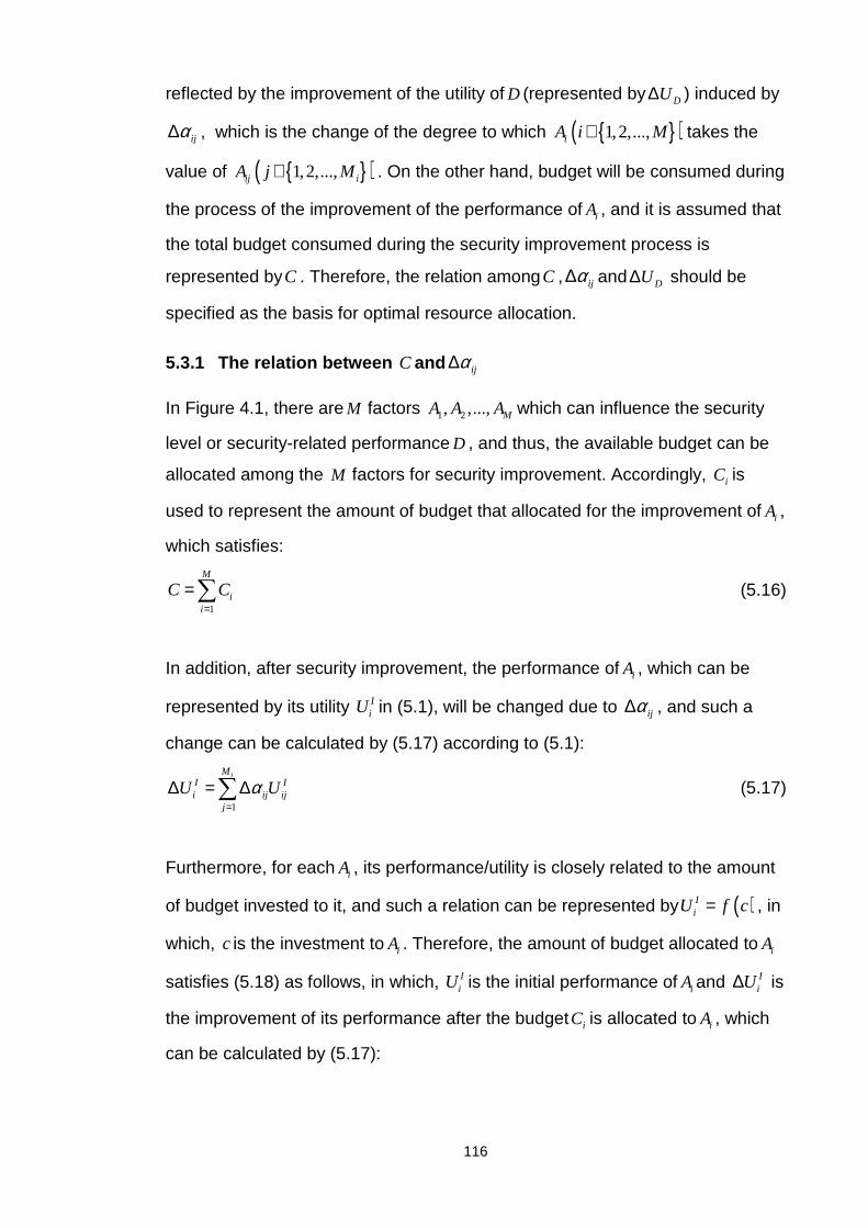
116
reflected by the improvement of the utility of D (represented by DU∆ ) induced by
ijα∆ , which is the change of the degree to which ( )1,2,...,iA i M∈ takes the
value of ( )1,2,...,ij iA j M∈ . On the other hand, budget will be consumed during
the process of the improvement of the performance of iA , and it is assumed that
the total budget consumed during the security improvement process is
represented byC . Therefore, the relation amongC , ijα∆ and DU∆ should be
specified as the basis for optimal resource allocation.
5.3.1 The relation between C and ijα∆
In Figure 4.1, there are M factors 1 2, ,..., MA A A which can influence the security
level or security-related performance D , and thus, the available budget can be
allocated among the M factors for security improvement. Accordingly, iC is
used to represent the amount of budget that allocated for the improvement of iA ,
which satisfies:
1
M
ii
C C=
=∑ (5.16)
In addition, after security improvement, the performance of iA , which can be
represented by its utility IiU in (5.1), will be changed due to ijα∆ , and such a
change can be calculated by (5.17) according to (5.1):
1
iMI Ii ij ij
j
U Uα=
∆ = ∆∑ (5.17)
Furthermore, for each iA , its performance/utility is closely related to the amount
of budget invested to it, and such a relation can be represented by ( )IiU f c= , in
which, c is the investment to iA . Therefore, the amount of budget allocated to iA
satisfies (5.18) as follows, in which, IiU is the initial performance of iA and I
iU∆ is
the improvement of its performance after the budget iC is allocated to iA , which
can be calculated by (5.17):
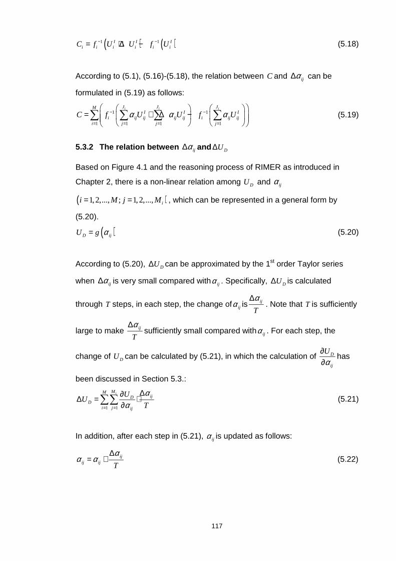
117
( ) ( )1 1I I Ii i i i i iC f U U f U− −= + ∆ − (5.18)
According to (5.1), (5.16)-(5.18), the relation between C and ijα∆ can be
formulated in (5.19) as follows:
1 1
1 1 1 1
i i iJ J JMI I I
i ij ij ij ij i ij iji j j j
C f U U f Uα α α− −
= = = =
= + ∆ −
∑ ∑ ∑ ∑ (5.19)
5.3.2 The relation between ijα∆ and DU∆
Based on Figure 4.1 and the reasoning process of RIMER as introduced in
Chapter 2, there is a non-linear relation among DU and ijα
( )1,2,..., ; 1,2,..., ii M j M= = , which can be represented in a general form by
(5.20).
( )D ijU g α= (5.20)
According to (5.20), DU∆ can be approximated by the 1st order Taylor series
when ijα∆ is very small compared with ijα . Specifically, DU∆ is calculated
through T steps, in each step, the change of ijα is ij
T
α∆. Note that T is sufficiently
large to make ij
T
α∆sufficiently small compared with ijα . For each step, the
change of DU can be calculated by (5.21), in which the calculation of D
ij
U
α∂∂
has
been discussed in Section 5.3.:
1 1
iMMijD
Di j ij
UU
T
αα= =
∆∂∆ = ⋅∂∑∑ (5.21)
In addition, after each step in (5.21), ijα is updated as follows:
ijij ij T
αα α
∆= + (5.22)

118
The above process indicated by (5.21) and (5.22) is repeated for T times to
generate DU∆ induced by ( )1,2,..., ; 1,2,...,ij ii M j Mα∆ = = .
5.3.3 Maximize security improvement under the const raint on budget
In this situation, it is assumed that the total budget to increase initial security
level isC , and the question is how to allocateC among ( )1,2,...,iA i M= to
maximize the increase of DU in Figure 4.1, in other words, how to determine the
value of ijα∆ so that DU∆ can be maximized under the constraint of C according
to the relation among C , ijα∆ and DU∆ .
In real applications, the improvement of iA not only depends on available budget,
it also depends on other factors, such as available human resources, current
technology capability, etc. Therefore, besides the constraints on budget, there
may be also certain constraints on ijα∆ due to the limitation on other factors,
and such constraints can only be determined when specific problems are
analyzed in detail.
Therefore, the optimization model is built as follows to solve this problem with
( )1,2,..., ; 1,2,...,ij ii M j Mα∆ = = be the decision variables.
( )max D ijU f α∆ = ∆ (5.23)
Subject to:
1 1
1 1 1 1
i i iJ J JMI I I
i ij ij ij ij i ij iji j j j
f U U f U Cα α α− −
= = = =
+ ∆ − ≤
∑ ∑ ∑ ∑ (5.24)
( )1
0 1,2,...,iM
ijj
i Mα=
∆ = =∑ (5.25)
( )1,2,..., ; 1,2,...,oU oLij ij ij ii M j Mα α α≤ ∆ ≤ = = (5.26)
( )1 1,2,..., ; 1,2,...,ij ij ij ii M j Mα α α− ≤ ∆ ≤ − = = (5.27)
In the above model, DU∆ in (5.23) is a function of ijα∆ which can be specified by
the process discussed in section 5.4.2, (5.24) is the constraint on total budget
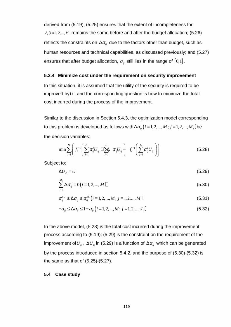
119
derived from (5.19); (5.25) ensures that the extent of incompleteness for
( )1,2,...,iA i M= remains the same before and after the budget allocation; (5.26)
reflects the constraints on ijα∆ due to the factors other than budget, such as
human resources and technical capabilities, as discussed previously; and (5.27)
ensures that after budget allocation, ijα still lies in the range of [ ]0,1 .
5.3.4 Minimize cost under the requirement on securi ty improvement
In this situation, it is assumed that the utility of the security is required to be
improved byU , and the corresponding question is how to minimize the total
cost incurred during the process of the improvement.
Similar to the discussion in Section 5.4.3, the optimization model corresponding
to this problem is developed as follows with ( )1,2,..., ; 1,2,...,ij ii M j Mα∆ = = be
the decision variables:
1 1
1 1 1 1
mini i iJ J JM
I Ii ij ij ij ij i ij ij
i j j j
f U U f Uα α α− −
= = = =
+ ∆ −
∑ ∑ ∑ ∑ (5.28)
Subject to:
DU U∆ = (5.29)
( )1
0 1,2,...,iM
ijj
i Mα=
∆ = =∑ (5.30)
( )1,2,..., ; 1,2,...,oU oLij ij ij ii M j Mα α α≤ ∆ ≤ = = (5.31)
( )1 1,2,..., ; 1,2,...,ij ij ij ii M j Jα α α− ≤ ∆ ≤ − = = (5.32)
In the above model, (5.28) is the total cost incurred during the improvement
process according to (5.19); (5.29) is the constraint on the requirement of the
improvement of DU , DU∆ in (5.29) is a function of ijα∆ which can be generated
by the process introduced in section 5.4.2, and the purpose of (5.30)-(5.32) is
the same as that of (5.25)-(5.27).
5.4 Case study
120
In the discussion in previous chapters, cargo theft in port storage area is one of
the most common threats faced by CLSC operation, and a model for security
assessment of a port along a CLSC against cargo theft is developed in Chapter
3 while the security level of different ports are assessed by RIMER in Chapter 4
based on the model and the data collected from the ports.
In the security assessment model, various factors related to port security
against cargo theft are identified, and among the factors, the performance of
access control system is very important, as access control system is one of the
key elements to prohibit unauthorized access to cargo storage areas (Knight,
2003). Therefore, in this case study, the performance of an access control
system of a port in China is assessed first, based on which the available budget
is allocated among the relevant basic factors according to the model developed
in this chapter to improve its performance in an effective and efficient way.
According to the security assessment model proposed in Chapter 3, 3 basic
factors are used to measure the performance of an access control system in a
port:
• Coverage of access control system: revealing the areas protected by the
access control system
• Robustness of access control system: indicating whether the access
control system is reliable or not
• Capability of access control system: reflected by the way that the access
points are controlled
In addition, as discussed in Chapter 3, to accommodate different forms of
information with different kinds of uncertainty existing in the basic factors of the
security assessment model, belief distributions are used to measure the basic
factors. According to Appendix 2, regarding the performance of access control
system, the grades/referential values used to describe its basic factors and the
meaning of each grade/referential value is shown in Table 5.1.
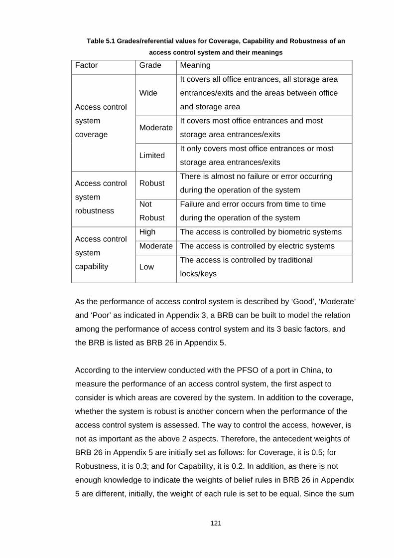
121
Table 5.1 Grades/referential values for Coverage, Capability and Robustness of an
access control system and their meanings
Factor Grade Meaning
Access control
system
coverage
Wide
It covers all office entrances, all storage area
entrances/exits and the areas between office
and storage area
Moderate It covers most office entrances and most
storage area entrances/exits
Limited It only covers most office entrances or most
storage area entrances/exits
Access control
system
robustness
Robust There is almost no failure or error occurring
during the operation of the system
Not
Robust
Failure and error occurs from time to time
during the operation of the system
Access control
system
capability
High The access is controlled by biometric systems
Moderate The access is controlled by electric systems
Low The access is controlled by traditional
locks/keys
As the performance of access control system is described by ‘Good’, ‘Moderate’
and ‘Poor’ as indicated in Appendix 3, a BRB can be built to model the relation
among the performance of access control system and its 3 basic factors, and
the BRB is listed as BRB 26 in Appendix 5.
According to the interview conducted with the PFSO of a port in China, to
measure the performance of an access control system, the first aspect to
consider is which areas are covered by the system. In addition to the coverage,
whether the system is robust is another concern when the performance of the
access control system is assessed. The way to control the access, however, is
not as important as the above 2 aspects. Therefore, the antecedent weights of
BRB 26 in Appendix 5 are initially set as follows: for Coverage, it is 0.5; for
Robustness, it is 0.3; and for Capability, it is 0.2. In addition, as there is not
enough knowledge to indicate the weights of belief rules in BRB 26 in Appendix
5 are different, initially, the weight of each rule is set to be equal. Since the sum

122
of the rule weights is 1, for each rule, the weight is 0.056. Note that to increase
the performance of the assessment model, i.e., to make the assessment result
closer to reality, the parameters specified above can be trained and updated
using the algorithm proposed by Yang et al. (2007) when more data regarding
the relation among the performance of the access control system and its 3 basic
factors become available.
After the knowledge about the relation among the performance of an access
control system and its 3 basic factors is acquired and structured by a BRB, the
information regarding the 3 basic factors should be collected based on the real
situation of the port.
According to the PFSO’s response of the questionnaire regarding security
against cargo theft, and the information collected during the follow-up interview
with the PFSO, the features of the assess control system in the port can be
summarized as follows:
• The access control system covers all the office entrances, however, most
of the entrances/exits of storage area, i.e., the container yard in the port,
which is a very large piece of land, is not equipped with access control
system;
• The access is controlled by both electronic system and the traditional
locks/keys, for example, the main entrances of the buildings are
controlled by electronic systems while the access points within the
buildings, e.g., office doors, are controlled by conventional keys/locks.
However, it is difficult to find out how many access points are controlled
by electronic system and traditional locks/keys respectively.
• The overall robustness of the access control system is satisfactory, and
for the robustness of the electronic access control system, it is very good,
as the system has run for years without any failures or errors.
According to the above statements and the grades defined in Table 5.1, the
Coverage, Capability and Robustness of the access control system can be
measured by the belief distribution as follows:

123
• Coverage: (Wide, 0.1), (Moderate, 0.1), (Limited, 0.8);
• Robustness: (High, 0.8), (Low, 0.2);
• Capability: (High, 0), (Moderate, 0.5), (Low, 0.5).
Note that, regarding the Capability, according to the port’s real situation, the
belief degrees assigned to both the grade of ‘Medium’ and the grade of ‘Low’
may take any value within the interval of[ ]0,1 , and in this case study, the
average value of the lower and upper boundary of the interval is considered as
a representative value of the belief degree.
According to the information regarding the 3 basic factors measured in belief
distribution as above and BRB 26 in Appendix 5, RIMER can be applied to
generate the assessment result of the performance of the access control
system, and the result is represented by (Good, 0.1399), (Moderate, 0.3771),
(Poor, 0.4830). Further, if the utility of ‘Good’, ‘Moderate’ and ‘Poor’ are 1, 0.5
and 0 respectively, the overall utility of the performance of the access control
system is 0.3285.
As indicated by the PFSO, such a performance is certainly not satisfactory, to
ensure an effective protection against cargo theft in the port, the utility should
be around 0.7 at least. Therefore, a natural question arises as how to minimize
the total cost to satisfy the requirement on the improvement of utility.
According to current situations in the port, potentially, the following alternatives
can be applied to improve the basic factors:
• For Coverage: equip access control system to the whole container yard;
• For Robustness: improve the reliability of conventional locks and keys, if
biometric systems are introduced, ensure the high reliability of the
biometric system;
124
• For Capability: install more electronic access control systems, and
introduce biometric systems into access control if possible, reduce the
number of conventional locks/keys.
In addition, according to the PFSO’s experience, the following set of equations
can be used to roughly reflect the relations between the amount of money
invested and the utility of the 3 factors:
( )( )log 1 1,2,3i
Ii aU C i= + = (5.33)
In (5.33), IiU is the utility of the ith basic factor, which can be calculated by (5.1),
and C is the necessary cost or investment to generate the utility of IiU , which
satisfies 0 1iC a≤ ≤ − , in which, ia is a parameter with 1ia > .
According to (5.33), the following conclusion can be drawn:
• When 0C = , 0IiU = , indicating that the utility of the factor is 0 with no
investment.
• The first derivative of IiU regarding C is
( )1
1 ln
Ii
i
dU
dC C a=
+. Since 1ia > ,
0IidU
dC> , showing that the utility of the basic factor increases with the
increase of investment.
• The second derivative of IiU regarding C is
( )2
22
1
1 lni
i
d U
dC C a= −
+. As 1ia > ,
2
20id U
dC< , which reveals that the increasing rate of I
iU decreases with the
increase ofC , i.e., the impact of the same amount of investment on the
utility of the 3 basic factors decreases with the increase of the investment.
• As 0 1iC a≤ ≤ − , we have 0 1iU≤ ≤ , indicating that the utility of the factor
is between 0 and 1.

125
If the Coverage, Robustness and Capability are considered as the first, the
second and the third basic factor, according to the belief distributions used to
describe the 3 basic factors as discussed earlier, we have:
11 12 130.1, 0.1, 0.8;α α α= = =
21 220.8, 0.2;α α= =
31 32 330, 0.5, 0.5α α α= = =
In addition, if in (5.1), 11 21 31 12 32 13 22 331; 0.5; 0I I I I I I I IU U U U U U U U= = = = = = = = , we
have:
1 2 30.15, 0.8, 0.25I I IU U U= = =
Furthermore, as it is estimated by the PFSO that to make the utility of Coverage,
Robustness and Capability to be 1, about $10,000, $1,000 and $100,000 is
needed, according to (5.33), we have:
1 2 310,000, 1,000, 100,000a a a= = = .
On the other hand, for all 3 basic factors, the improvements are reflected by the
change of ( )1 2 31,2,3; 1,..., ; 3, 2, 3ij ii j M M M Mα∆ = = = = = . As discussed
previously, the constraints on ijα∆ not only depend on the requirements on
belief degrees in belief distributions, they also depend on the characteristics of
individual factors and specific situation of the port. For example, as indicated by
the PFSO, it is better that the improvement of the access control system can be
finished within the next financial year. Thus, it is unlikely that the whole area
within the port can be covered by the access control system within the time
constraint, and correspondently, the improvement of the basic factor of
Coverage has a set of constraints because of the limited time period, and the
constrains are:
11 12 130 0.7, 0.1 0.7, 0.8 0α α α≤ ∆ ≤ − ≤ ∆ ≤ − ≤ ∆ ≤
Regarding the improvement of Robustness, 21α∆ should be above 0 to make the
improvement possible, and on the other hand, it is very demanding that “there is

126
almost no failure or error occurring during the operation”, especially regarding
conventional locks/keys, thus, it is unlikely that 21α can take the value of 1, i.e.,
21α∆ is assumed to be less than 0.1. Therefore, we have:
21 220 0.1, 0.1 0α α≤ ∆ ≤ − ≤ ∆ ≤
In addition, due to the lack of technical capacity in the port, it is difficult to equip
all the access points of the terminal with biometric systems. Correspondently,
the constraints regarding ( )3 1,2,3j jα∆ = are:
31 32 330 0.6, 0.5 0.5, 0.5 0α α α≤ ∆ ≤ − ≤ ∆ ≤ − ≤ ∆ ≤
According to the above discussions, the problem of minimizing the cost to meet
the requirement of performance improvement of the access control system in
the port can be formulated as follows with ijα∆ be decision variables:
( )1 2 31,2,3; 1,..., ; 3, 2, 3ii j M M M M= = = = = :
3
1
min ii
C=∑ (5.34)
Subject to:
0.3715OU U∆ = = (5.35)
11 12 13 0α α α∆ + ∆ + ∆ = (5.36)
21 22 0α α∆ + ∆ = (5.37)
31 32 33 0α α α∆ + ∆ + ∆ = (5.38)
110 0.7α≤ ∆ ≤ (5.39)
120.1 0.7α− ≤ ∆ ≤ (5.40)
130.8 0α− ≤ ∆ ≤ (5.41)
210 0.1α≤ ∆ ≤ (5.42)
220.1 0α− ≤ ∆ ≤ (5.43)
310 0.6α≤ ∆ ≤ (5.44)
320.5 0.5α− ≤ ∆ ≤ (5.45)
330.5 0α− ≤ ∆ ≤ (5.46)

127
In (5.34), ( )1,2,3iC i = can be calculated as follows:
( ) ( )1 1 1 10.15 0.151 1 11 1 10000 10000
i i i iU U U UC a a+∆ +∆= − − − = − (5.47)
( ) ( )2 2 2 20.8 0.22 2 21 1 1000 1000
I I I IU U U UC a a+∆ +∆= − − − = − (5.48)
( ) ( )3 3 3 30.25 0.253 3 31 1 100000 100000
I I I IU U U UC a a+∆ +∆= − − − = −
(5.49)
In (5.35), oU∆ is a function of ijα∆ which can be specified by the process
discussed in section 5.4.2, while 1IU∆ , 2
IU∆ and 3IU∆ in (5.47)-(5.49) can be
generated as follows:
1 11 11 12 12 13 13 11 120.5I I I IU U U Uα α α α α∆ = ∆ + ∆ + ∆ = ∆ + ∆ (5.50)
2 21 21 22 22 21I I IU U Uα α α∆ = ∆ + ∆ = ∆ (5.51)
3 31 31 32 32 33 33 31 320.5I I I IU U U Uα α α α α∆ = ∆ + ∆ + ∆ = ∆ + ∆ (5.52)
In the above model from (5.34) to (5.52), (5.34) is the objective function, aiming
at minimizing the cost incurred during the security improvement process; (5.35)
specifies the requirement for security improvement based on the security
assessment result; the aim of (5.36)-(5.38) is to ensure the extent of
incompleteness in the original information regarding the 3 basic factors
unchanged before and after improvement; (5.39)-(5.46) are the constraints on
the change of belief degrees assigned to different grades/referential values
used to describe the 3 basic factors, as discussed previously; (5.47)-(5.49) are
used to calculate the cost incurred during the improvement of each basic factor;
while (5.50)-(5.52) are the equations to calculate the change of utility of each
basic factor.
According to the model from (5.34) to (5.52), the optimal solution can be
generated by directly using the fmincon function in Matlab as follows with the
parameterT in (5.21) and (5.22) taking the value of 100:
11 12 130.2478, 0.5522, 0.8α α α∆ = ∆ = ∆ = −
21 220.0987, 0.0987α α∆ = ∆ = −
31 32 330.2512, 0.2134, 0.4846α α α∆ = ∆ = ∆ = −

128
Therefore, the belief distributions used to describe the 3 basic factors regarding
the performance of the access control system after improvement are:
• Coverage: (Wide, 0.3478), (Medium, 0.6522), (Limited, 0)
• Reliability: (High, 0.8987), (Low, 0.1013)
• Capability: (High, 0.2512), (Moderate, 0.7334), (Low, 0.0154)
Correspondently, the performance of the access control system is described by
the following belief distributions:
(Good, 0.4274), (Moderate, 0.5336), (Poor, 0.0389)
Thus, the utility of the performance of the access control system is 0.6943,
which is very close to 0.7, while the cost incurred during the improvement
process is $1949, with 1 492C = , 2 246C = and 3 1211C = .
The above solution indicates that, to improve the performance of the access
control system in the port based on its current status, the following actions
should be taken to minimize the cost incurred during the improvement process:
• Regarding Coverage: the access control system should be equipped to
cover most storage areas’ entrances/exits;
• Regarding Capability: more than 70% of the access control points should
be controlled by electronic key-cards, the number of the access points
controlled by traditional key-locks should be reduced significantly, and
some of the access control points (around 25%), possibly access control
points to some critical areas, should be controlled by biometric
information;
• Regarding capability: the robustness of newly installed biometric access
control equipments should be good
In summary, in the case study, the resource allocation model proposed in this
chapter is applied to minimize the cost incurred for performance improvement of
129
an access control system in a port to prevent cargo theft. Specifically, different
amount of budgets are allocated to different basic factors regarding the access
control system performance, and the solution of the model can provide a set of
detailed suggestions for the PFSO on how the improvement can be conducted.
More generally, the resource allocation model proposed in this chapter can be
used for optimal resource allocation for security improvement of the whole port
or other organizations along a CLSC against various threats. In addition, the
model can be even applied in a broader and more macro level, e.g., funding
allocation among different departments or regions in a country based on risk or
security assessment result.
5.5 Conclusion
In this chapter, a set of new models to optimally allocate resources to improve
CLSC security based on security assessment result is proposed. The models
can be used to solve the following 2 categories of resource allocation problems:
1) how to minimize cost under the requirement on security improvement; and 2)
how to maximize security improvement under the constraints on available
resources.
Different from the existing resource allocation models, the models proposed in
this paper has 2 major unique features. 1) The models in this chapter intend to
allocate resources in an optimal way based on security assessment results.
With security assessment results as a basis, resources can be allocated in a
more effective and efficient way in the sense that they can be allocated to areas
according to their priorities identified from the security assessment results. Such
prioritised resource allocation is important wherever available resources are
limited compared with the demand of the resources, e.g., security improvement
of CLSC. 2) The resource allocation model is based on the scheme of RIMER,
which can not only provide a unified framework to accommodate different forms
of information with different kinds of uncertainty but also provide a semi-
structured framework for knowledge modelling. Such a feature is important
when the models are applied in the context of CLSC, as the security-related
130
factors in CLSC may have different features with different kinds of uncertainty
and the knowledge regarding the relation among the security level and the
security-related factors may be difficult to be modelled in a purely structured
way. Therefore, the basis of RIMER makes the resource allocation more
rational and robust.
To test the applicability of the models proposed in the paper, a case study is
conducted regarding the resource allocation to improve the performance of an
access control system in a port to prevent cargo theft. The objective of the case
study is to minimize the cost incurred during the improvement process under
the requirement on performance improvement according to security assessment
result. Based on the solution of the model, a set of specific operations are
suggested to make use of the budget effectively and efficiently.
In addition, the model proposed in this chapter can be generalized for optimal
resource allocation for security improvement of the whole port or other
organizations involved in a CLSC. Further, apart from CLSC, the models also
have the potential to be applied into other areas with great complexity and
uncertainty, such as resource allocation to increase security against terrorism,
resource allocation to reduce risk in large enterprises, resource allocation to
reduce risk in developing new products with high novelty, and so on.
131
6 Chapter 6 Handling Different Information Aggregatio n Patterns for Security Assessment of CLSC
Abstract
In this chapter, based on the security assessment model developed in Chapter
3 regarding a port storage area along a CLSC against cargo theft, different
patterns for information aggregation in the model are identified and analyzed
according to the relations among the factors with information to be aggregated,
and a set of methods are also proposed to handle the aggregation patterns
under the framework of RIMER. To validate the aggregation patterns identified
and the methods to handle the aggregation patterns, case studies based on the
data collected from different ports in both the UK and China are conducted in
this chapter.
6.1 Introduction
In Chapter 3 and Chapter 4, an analytical model is proposed for overall security
assessment of a CLSC and the model is then refined for security assessment of
a port storage area along a CLSC against cargo theft. Specifically, the security
assessment model organizes various factors relevant to CLSC security
hierarchically and the result of security assessment is generated by aggregating
information of the factors from the lower level to upper level in the hierarchical
model. Although RIMER is capable of accommodating and handling information
in different forms with different kinds of uncertainty, it aggregates information in
a single fixed way regardless of the fact that the nature of relations among the
factors with information to be aggregated may be inherently different. Therefore,
a set of patterns to aggregate information of different factors should be
developed according to the nature of the relations among the factors.
Facing the situation mentioned above, this chapter intends to analyze the
relations among the factors in the security assessment model in Appendix 1 in
detail, and according to the nature of such relations, a set of information
aggregation patterns are identified. Further, the methods to aggregate
132
information in different patterns are also proposed under the framework of
RIMER.
6.2 Different aggregation patterns in security asse ssment model
The BRBs for the security assessment model developed in Chapter 3 are
shown in Appendix 5, from which, it can be seen that there are 36 BRBs in total.
Correspondently, the information regarding the antecedents in 36 BRBs should
be aggregated respectively, and the relationship among antecedents and
consequence of each BRB in Appendix 5 can be represented by Figure 4.1,
which is considered as a basic information aggregation unit.
As discussed in Chapter 4, in Figure 4.1, factor 1A to MA can be considered as
antecedents of a BRB while factor D can be considered as the corresponding
consequence in the BRB. On the other hand, under the context of information
aggregation, Figure 4.1 can be explained in another way as follows: within a
basic information aggregation unit, the information contained in factor 1A to MA is
aggregated to generate the information in factor D , and the factors with
information to be aggregated, i.e., factor 1A to MA in Figure 4.1, are referred to as
“parent factors” hereafter, while the factor with information generated by the
aggregation of parent factors, i.e., factor D in Figure 4.1, is referred to as “child
factor” hereafter. From the discussion in Chapter 4, it is known that factor D can
take N referential values, i.e., 1 2, ,..., ND D D and factor ( )1,2,...,iA i M= can take
iM referential values, i.e., 1 2, ,...,ii i iMA A A . As the features of the relation among a
child factor and its parent factors in different basic information aggregation units
may be various, it is inappropriate to aggregate information in different basic
units using the same pattern.
In general, according to the nature of relations among parent factors and their
common child factor, there are 2 patterns for information aggregation, i.e.,
heterogeneous aggregation and homogeneous aggregation, which are
explained as follows:

133
• In heterogeneous aggregation, the nature of each parent factor and that
of child factor are different, and the child factor is modelled by its parent
factors, the nature of the child factor will change if any of its parent
factors are missing. A typical example of this pattern of aggregation in
the security assessment model in Appendix 1 is the relation among the
factors of Security, Threat Likelihood, Potential Consequence and
Vulnerability. The 4 factors have different nature. Among the 4 factors,
Security is the child factor, which is modelled by the 3 parent factors. In
addition, all of the 3 parent factors are essential in modelling Security
and Security cannot be estimated if the information of any of the 3 parent
factors is missing.
• In homogeneous aggregation, child factor and parent factors share the
same nature, and child factor is composed of its parent factors, the
nature of the child factor will not change if some of its parent factors are
missing, however, in this case, the magnitude of the child factor may be
influenced. In homogeneous aggregation, it can be said that a parent
factor is ‘a part of’ or ‘a kind of’ a child factor. A typical example of this
pattern in the security assessment model in Appendix 1 is the relation
among the factors of Potential Consequence, Human Loss, Financial
Loss, Corporate Image Loss, Economic Loss and Environmental Loss.
All the 6 factors share the same nature, and among the 6 factors,
Potential Consequence is the child factor, which is composed of the
other 5 factors. In the aggregation process, if the information of any of
the 5 factors is missing, the aggregated factor can still be considered as
Potential Consequence, only the magnitude of Potential Consequence is
influenced. Further, any parent factor can be considered as ‘a kind of’
Potential Consequence.
Under each pattern introduced above, there are several sub-patterns. Before
the sub-patterns are introduced in detail, three kinds of factors, namely, ‘Effect
Influenced Factor (EIF)’, ‘Value Influenced Factor (VIF)’ and ‘Base Factor (BF)’,
which are crucial for the introduction of sub-patterns, are defined as follows:
134
• Effect Influenced Factor (EIF): in Figure 4.1, ( )1,2,...,iA i M∈ is an EIF
of ( )1,2,..., ,jA j M j i∈ ≠ regarding D if the effect of jA on D is influenced
by the referential value taken by iA . The set of 'jA s EIF can be
represented by ( )jEIF A . More specifically, there are 3 different
categories of EIF as introduced as follows:
o If there exists a pre-defined threshold iLt ( )0 1iLt< ≤ , when the utility
of iA is below iLt , the effect of jA on D is influenced, iA is the N-EIF
of jA , which means that low performance of iA cannot be
compensated by jA ;
o If there exists a pre-defined threshold iHt ( )0 1iHt≤ < , when the
utility of iA is above iHt , the effect of jA on D is influenced, iA is the
P-EIF of jA , which means that high performance of iA cannot be
offset by jA ;
o If there exists a pair of pre-defined thresholds iLt and iHt with
0 1iLt< ≤ and 0 1iHt≤ < , when the utility of iA is below iLt or above
iHt , the effect of jA on D is influenced, iA is the C-EIF of jA , which
means that jA can neither compensate 'iA s low performance nor
offset 'iA s high performance
• Value Influenced Factor (VIF): in Figure 4.1, ( )1,2,...,iA i M∈ is a VIF of
( )1,2,..., ,jA j M j i∈ ≠ if in general, the probability of jA taking its
referential value ( )1,2,...,jjm j jA m M∈ is influenced by the referential
value taken by iA . The set of 'jA s VIF can be represented by ( )jVIF A .
Note that, if ( )i jA VIF A∈ , then ( )j iA VIF A∉ ;
• Base Factor (BF): in Figure 4.1, ( )1,2,...,iA i M∈ is a BF of
( )1,2,..., ,jA j M j i∈ ≠ if under a certain situation, the extent to which jA
can be described by its referential value ( )1,2,...,jjm j jA m M∈ is
135
dependent on the referential value taken by iA . The set of 'jA s BF can be
represented by ( )jBF A , and if ( )i jA BF A∈ , then ( )j iA BF A∉ .
Note that, the difference between VIF and BF is that: if iA is a VIF of jA , what is
influenced is the probability that jA takes a certain referential value in general,
but under a certain situation, jA can take its referential values to any appropriate
extent; if iA is a BF of jA , in general, jA can take any of its referential values with
any appropriate probability, what is influenced is the extent to which jA can be
described by a certain referential value under a specific situation. The difference
will be further elaborated with the examples in subsequent sections.
In addition, to facilitate the following discussions, the following features are also
defined based on Figure 4.1:
• Feature-HET: Child factor D is modelled by parent factors 1 2, ,..., MA A A ,
the information of D is generated by aggregation of information of
( )1,2,...,iA i M= . None of iA is ‘a part of’ or ‘a kind of’ D , and the nature
of D will change if the information of any of parent factor iA is missing
• Feature-HOM: Child factor D is composed of parent factors 1 2, ,..., MA A A ,
in addition, D , 1 2, ,..., MA A A have the same nature, and ( )1,2,...,iA i M=
can be considered as ‘a part of’ or ‘a kind of’ D . The nature of D will not
change if the information of any of parent factor iA is missing, although
the magnitude of D will be influenced in this case
• Feature-EIF-0: For any ( )1,2,...,iA i M∈ , ( )iEIF A φ= , i.e., the impact of
low/high performance of any parent factor iA can always be
compensated/offset by the other parent factors ( )1,2,..., ;jA j M j i∈ ≠
• Feature-EIF-1: For some parent factor ( )1,2,...,iA i M∈ , ( )iEIF A φ≠ ,
and ( ) ( )1,2,..., 1i i iEIF A E E M= ∈ − . Further, the elements in ( )iEIF A

136
are represented as 1 2, ,...,ii i iEA A A , with 1 2, ,...,
iie MA A A A∈ and
( )1,2,...,iie i i iA A e E≠ =
• Feature-EIF-2: In total, there are P factors which are EIFs of other factors,
and such P factors are represented by: ( ) 1 21
, ,...,M
i E E EPi
EIF A A A A=
=∪ , in
which ( )1 2, ,..., 1,2,...Ep MA A A A p P∈ =
• Feature-VIF-0: For any ( )1,2,...,iA i M∈ , ( )iVIF A φ= , i.e., in general,
the probability that iA takes its referential value is not influenced by
referential values taken by other parent factors ( )1,2,..., ;jA j M j i∈ ≠
• Feature-VIF-1: For some parent factor ( )1,2,...,iA i M∈ , ( )iVIF A φ≠ ,
and ( ) ( )1,2,..., 1i i iVIF A V V M= ∈ − . Further, the elements in ( )iVIF A
are represented as: 1 2, ,...,ii i iVA A A , with 1 2, ,...,
iiv MA A A A∈ and
( )1,2,...,iiv i i iA A v V≠ =
• Feature-VIF-2: In total, there areQ factors which are VIFs of other factors,
and suchQ factors are represented by: ( ) 1 21
, ,...,M
i V V VQi
VIF A A A A=
=∪ , in
which ( )1 2, ,..., 1,2,...Vq MA A A A q Q∈ =
• Feature-VIF-3: The relation among iA and the elements in ( )iVIF A is built
by the probability of iA taking a certain referential value conditional on the
combinations of the referential values taken by the elements in ( )iVIF A ,
i.e., ( )1 2| , ,...ii i i iVP A A A A
• Feature-BF-0: for any ( )1,2,...,iA i M∈ , ( )iBF A φ= , i.e., under a specific
situation, the extent to which iA can take a certain referential value is not
influenced by the referential values taken by ( )1,2,..., ;jA j M j i∈ ≠
• Feature-BF-1: for some parent factor ( )1,2,...,iA i M∈ , ( )iBF A φ≠ , and
( ) ( )1,2,..., 1i i iBF A B B M= ∈ − . Further, the elements in ( )iBF A are
137
represented as: 1 2, ,...,ii i iBA A A , with ( )1 2, ,..., 1,2,...,
iib M i iA A A A b B∈ ∈ and
iib iA A≠
• Feature-BF-2: In total, there are R factors which are BFs of other factors,
and such R factors are represented by: ( ) 1 21
, ,...,M
i B B BRi
BF A A A A=
=∪ , in
which ( )1 2, ,..., 1,2,...Br MA A A A r R∈ =
• Feature-BF-3: the relation among iA and the elements in ( )iBF A is
dependent on the features of a certain basic information aggregation unit
according to specific knowledge contained in the unit;
6.2.1 Aggregate information under heterogeneous pat tern
In the security assessment model in Appendix 1, the simplest pattern to
aggregate information heterogeneously is based on the fact that there is no EIF,
VIF or BF involved in the information aggregation. In the example mentioned
previously regarding the relation among the factors of Security, Threat
Likelihood, Potential Consequence and Vulnerability, the effect of low/high utility
of any parent factor on the child factor can be compensated/offset by the
high/low utility of other parent factors, the probability that one parent factor
taking its referential values in general is independent of the referential values
taken by other parent factors, and the extent to which a parent factor can be
described by a certain referential value under a certain situation is not
influenced by the referential values taken by other parent factors. More
generally, the features of such an aggregation pattern include: Feature-HET,
Feature-EIF-0, Feature-VIF-0 and Feature-BF-0, and the aggregation pattern
with the features below is referred to as ‘HET-N’ in the rest of the thesis
The above aggregation pattern is based on the fact that within a basic unit for
information aggregation as indicated in Figure 4.1, the impact of any parent
factor on child factor can always be compensated or offset by other parent
factors. However, it is possible that the performance of a parent factor cannot
be compensated or offset by other parent factors in some heterogeneous
information aggregation problems, although there is no such example in the
security assessment model in Appendix 1. The general feature of the

138
heterogeneous aggregation pattern with EIF(s) include Feature-HET, Feature-
EIF-1, Feature-EIF-2, Feature-VIF-0 and Feature-BF-0, and such an
aggregation pattern is referred to as ‘HET-E’ in the rest of the thesis:
In a basic unit for information aggregation in Figure 4.1, it is also possible that
( )iVIF A φ≠ for some factors ( )1,2,...iA i M∈ , i.e., in general, the probability
that iA takes its referential values is influenced by the referential values taken by
( )1, 2,..., ,jA j M j i∈ ≠ . However, there is no example of this aggregation pattern
in the security assessment model in Appendix 1. Generally, the features of
heterogeneous aggregation pattern with VIF(s) include Feature-HET, Feature-
VIF-1, Feature-VIF-2, Feature-VIF-3, Feature-EIF-0 and Feature-BF-0, and the
aggregation pattern is referred to as ‘HET-V’ in the rest of the thesis:
Under the heterogeneous aggregation pattern, there is another situation in
which the extent that a factor iA takes its referential values is influenced by the
referential values taken by other factors ( )1,2,..., ,jA j M j i∈ ≠ , and this
situation is referred to as ‘HET-B’ hereafter in the thesis. Based on Figure 4.1,
the features of such a pattern include Feature-HET, Feature-BF-1, Feature-BF-
2, Feature-BF-3, Feature-EIF-0 and Feature-VIF-0.
Further, it is also possible that for heterogeneous information aggregation,
factors with EIF, VIF and BF may coexist with each other. Such a pattern can
be referred to as ‘HET-C’, and the features of such a pattern include Feature-
HET and one or more of the following groups of features:
• Group 1: Feature-EIF-1, Feature-EIF-2
• Group 2: Feature-VIF-1, Feature-VIF-2, Feature-VIF-3
• Group 3: Feature-BF-1, Feature-BF-2, Feature-BF-3
6.2.2 Aggregate information under homogeneous patte rn
Another broad category of information aggregation is homogeneous
aggregation, in which, child factor has the same nature as all its parent factors.

139
Corresponding to 5 different sub-patterns under the heterogeneous pattern,
there are 5 sub-patterns under the homogeneous pattern. Among which, the
most simple pattern is the one with no parent factor having EIF, VIF or BF. For
example, in the security assessment model in Appendix 1, there is a basic unit
containing the factors of Hardware Facility, Control Facility and Monitor Facility.
All the factors have the same nature: the facility of different hardware; and
further, low/high performance of one parent factor can always be
compensated/offset by high/low performance of the other parent factor; in
addition, in general, each parent factor can take its referential values with any
appropriate probabilities independently and the extent to which a parent factor
can be described by any of its referential value under a certain situation is not
influenced by referential values taken by the other parent factor. More generally,
the aggregation pattern of this category, which is referred to as “HOM-N”
hereafter, can be described by the following features: Feature-HOM, Feature-
EIF-0, Feature-VIF-0 and Feature-BF-0.
Another sub-pattern for homogeneous information aggregation is based on the
fact that there are some parent factors with EIF(s). For example, in the security
assessment model in Appendix 1, among the factors of Intervention Measures
(IM), Preventative Measures (PM), Responsive Measures (RSM) and Recovery
Measures (RCM), the 3 parent factors (PM, RSM and RCM) share the same
nature with the child factor (IM), and each parent factor can be considered as ‘a
kind of’ child factor. In addition, as PM are the measures taken to prevent cargo
theft from happening, while both RSM and RCM are the measures taken to
minimize consequence after cargo theft already happen, PM are more crucial
than the other 2 categories of measures. Specifically, if the utility of PM is lower
than a pre-defined threshold, i.e., if PM are not effective enough, the utility of IM
will be limited, i.e., IM will also be ineffective regardless of the referential values
taken by RSM and RCM, and thus the low utility of PM cannot be compensated
by high utility of the other 2 parent factors. From the discussion, it can be seen
that PM is an EIF of both RSM and RCM. In addition, among PM, RSM and
RCM, in general, each factor can take its referential values with any appropriate
probabilities independently and under a specific situation, the extent to which a

140
parent factor can be described by any of its referential value is independent of
the referential values taken by other parent factors, thus there is no VIF or BF
involved in the aggregation process. In a more general way, such an
aggregation pattern, which is referred to “HOM-E” hereafter, can be
characterized by Feature-HOM, Feature-EIF-1, Feature-EIF-2, Feature-VIF-0
and Feature-BF-0.
Under the homogeneous aggregation pattern, it is also possible that some
parent factors have VIF(s). An example in the security assessment model in
Appendix 1 can be found in the basic unit containing the factors of Physical
Feature (PF), Historic Feature (HF), Employee Feature (EF) and Facility
Feature (FF). All 3 parent factors (HF, EF and FF) have the same nature as the
child factor (PF), and any parent factor can be considered as ‘a kind of’ child
factor. In addition, when HF is ‘Poor’, which indicates that theft happened
frequently in the port storage area in history, in general, both PF and EF may be
more likely to take the value of ‘Poor’ than ‘Good’. In this case, HF is a VIF of
both PF and EF. However, for a certain security assessment in a certain port,
the extent to which PF can be described by any of its referential values only
depends on the situation of the port at the time of security assessment, it is not
influenced by the referential value taken by HF, for example, for a port with
‘Poor’ HF, PF can be ‘Good’ to a large extent at the time when a certain security
assessment is conducted although in general, the probability that PF is ‘Good’
is low if HF is ‘Poor’. Therefore, HF is not a BF of PF. Similarly, HF is not a BF
of EF either. Furthermore, in this example, as low/high performance of one
parent factor can always be compensated/offset by high/low performance of
other parent factors, there is no EIF existing in this example. More generally,
this aggregation pattern is referred to as “HOM-V” hereafter, and its features
include Feature-HOM, Feature-VIF-1, Feature-VIF-2, Feature-VIF-3, Feature-
EIF-0 and Feature-BF-0.
Although there is no such example in the security assessment model in
Appendix 1, for homogeneous aggregation pattern, it is possible that some of
the child factors have BFs and no child factor have EIF or VIF. The
corresponding features include: Feature-HOM, Feature-BF-1, Feature-BF-2,
141
Feature-BF-3, Feature-EIF-0 and Feature-VIF-0. The aggregation pattern with
the above features is referred to as “HOM-B” hereafter in this thesis.
Besides the patterns introduced above, in the security assessment model in
Appendix 1, there is another pattern for homogeneous information aggregation,
in which, EIF, VIF and BF may coexist with each other. For example, in the
basic unit containing the factors of Operations relevant to Records (OR),
Keeping of Records (KR), Protection on Records (PR) and Management on
Records (MR), all the parent factors (OR, KR and MR) are ‘a kind of’ OR. In
addition, if KR is taking the referential value of ‘Yes’ to a degree of 0.8 and ‘No’
to a degree of 0.2, indicating that 20% of the records required in the security
assessment model are missing at the time of security assessment, both the
extent to which PR can take the referential value of ‘Yes’ and the extent to
which MR can take the referential value of ‘Well’ should be reduced by 20%,
since the protection and management cannot be applied to the missing records.
Therefore, if originally, PR and MR can be described by the referential value of
‘Yes’ and ‘Well’ to the degree of 1 respectively, with the consideration of the
impact of referential value taken by KR, PR should take its referential value of
‘Yes’ to a degree of 0.8 and ‘No’ to a degree of 0.2, while MR should take its
referential value of ‘Well’ to a degree of 0.8 and ‘Poor’ to a degree of 0.2.
Therefore, KR is the BF of both PR and MR. Note that, although the extent to
which MR is described by its referential values is influenced by the referential
values taken by KR in a specific security assessment as discussed above, the
general probabilities that MR can take any of its referential values are not
influenced by KR, in other words, MR has an equal chance to take both its
referential values in this case, as no matter how many records are missing for
the security assessment model, the management on the existing records can be
either ‘Well’ or ‘Poor’. Therefore, KR is not a VIF of MR, and similarly, KR is not
a VIF of PR either. On the other hand, as poor protection or poor management
on records will lead to unauthorized or inefficient access to the records, when
the utility of PR or MR is below a certain threshold, the effect of the other 2
parent factors to OR is influenced. In other words, the low performance of PR or
MR cannot always be compensated by the high performance of the other two
parent factors. Therefore, PR is an EIF of both KR and MR regarding OR while
142
MR is an EIF of both KR and PR regarding OR. The general features of the
information aggregation pattern in this category, which is referred to as ‘HOM-C’
hereafter, include Feature-HOM and one or more of the following groups of
features:
• Group 1: Feature-EIF-1, Feature-EIF-2
• Group 2: Feature-VIF-1, Feature-VIF-2, Feature-VIF-3
• Group 3: Feature-BF-1, Feature-BF-2, Feature-BF-3
A detailed list of information aggregation pattern for each group of factors in the
security assessment model in Appendix 1 with relevant explanations are
presented in Appendix 6.
6.3 Methods to handle different information aggrega tion patterns under the framework of RIMER
As revealed by the discussion in Chapter 2, RIMER is selected as a basis to
handle different information aggregation patterns. According to Section 6.2,
there are 2 broad categories of information aggregation patterns, i.e.,
homogeneous aggregation pattern and heterogeneous aggregation pattern, and
under each category, there are 5 sub-patterns for information aggregation.
Therefore, in this section, under the framework of RIMER, the methods to
handle the 2 broad categories of information aggregation patterns are
discussed first, followed by the methods to handle different sub-patterns
analyzed in Section 6.2.
6.3.1 Handling heterogeneous aggregation pattern an d homogeneous aggregation pattern
In homogeneous aggregation, as parent factors are ‘a part of’ or ‘a kind of’ child
factor, naturally, the impact of the combination of all parent factors on their child
factor can be generated by the sum of impact of each individual parent factor on
the child factor. On the other hand, in heterogeneous aggregation, as parent
factors have different nature with their child factor, it is more appropriate to
multiply the influence of each individual parent factor on the child factor to form
the influence of the combination of all parent factors on their child factor.

143
Therefore, from the methodological view, the difference between homogeneous
aggregation and heterogeneous aggregation can be reflected by different ways
to generate overall influence of the combination of all parent factors on their
child factor based on influence of each individual parent factor on the child
factor. Correspondently, under the context of BRB, for homogeneous
aggregation and heterogeneous aggregation, the way to generate belief
degrees in the consequence of belief rules based on the impact of each
individual antecedent on the consequence should be different.
In Chapter 4, a method to generate belief degrees in the consequence of belief
rules is proposed based on the impact of each individual antecedent on the
consequence. From (4.5), it can be seen that the impacts of each individual
antecedent on the consequence are multiplied to generate the impact of packet
antecedent on the consequence. According to discussion in previous paragraph,
such a method can be applied for heterogeneous information aggregation.
On the other hand, for homogeneous information aggregation, as it is more
appropriate to add up the impacts of each individual antecedent on
consequence to general the impact of packet antecedent on consequence, after
( )ji j jpP D D A A= = ( )1,2,..., ; 1,2,..., ; 1,2,...,j ji N j M p M= = = in Figure 4.1 is
generated by the process and method proposed in Chapter 4,
( )1 21 1 2 2, ,...,Mi p p M MpP D D A A A A A A= = = = can be calculated by (6.1) as follows
with the consideration of relative importance of jA , which is represented by
( )1,2,...,j j Mδ = :
( ) ( )1 21 1 2 21
, ,...,M j
M
i p p M Mp j i j jpj
P D D A A A A A A P D D A Aγ δ=
= = = = = = =∑ (6.1)
In (6.1), 1,2,...,
maxj
j
jj n
δδ
δ=
= , γ is a normalized factor to ensure
( )1 21 1 2 21
, ,..., 1M
N
i p p M Mpi
P D D A A A A A A=
= = = = =∑ .

144
As indicated in Chapter 4, to generate belief degrees in belief rules based on
the impact of individual antecedent on consequence instead of specifying such
belief degrees directly based on expert opinions can significantly reduce the
bias and inconsistency existing in the generation process. Moreover, it also
provides a framework to handle both heterogeneous and homogeneous
information aggregation pattern conveniently.
6.3.2 Handling aggregation pattern with EIF(s), VIF (s) and BF(s)
6.3.2.1 Aggregation pattern with EIF(s) On the basis of Figure 4.1 and according to the discussion in Section 6.2, when
iieA is an EIF of iA regarding D , with 1,2,...,i M∈ , 1,2,...,i ie E∈ ,
1,2,..., 1iE M∈ − , and when the utility of iieA satisfies some certain conditions,
the effect of iA on D will be restricted, i.e., the relative importance of iA regarding
D will reduce. According to Feature-EIF-1, for iA , there are iE EIF(s) in total, to
reflect the change on relative importance of iA caused by the existence of its
EIF(s), its attribute weight, iδ , can be updated as follows:
• If iieA is an N-EIF of iA :
( )1
min 1,i
i
i i
Eie
i ie ie L
U A
tδ δ
=
′ =
∏ (6.2)
• If iieA is a P-EIF of iA :
( )1
1min 1,
1
ii
i i
Eie
i ie ie H
U A
tδ δ
=
− ′ = −
∏ (6.3)
• If iieA is a C-EIF of iA :
( ) ( )1
1min ,1,
1
ii i
i i i
Eie ie
i ie ie L ie H
U A U A
t tδ δ
=
− ′ = −
∏ (6.4)
In (6.2) to (6.4), iδ ′ is the weight of iA after the impact of EIF is taken into
consideration; iie Lt and
iie Ht are the threshold ofiieA as defined in Section 6.2;
while the utility of ( )1,2,...,jA j M∈ can be calculated by (6.5) as follows:
( )1
j
j j
j
M
j jm jmm
U A u α=
= ∑ (6.5)
145
In (6.5), jjmu is the utility of ( )1,2,...,
jjm j jA m M= , which can be specified by
experts and satisfies 0 1jjmu≤ ≤ , and
jjmα is the degree to which factor jA takes
the value ofjjmA
Note that, (6.2) to (6.4) only represents one possible way to update antecedent
weight, there may be other ways for the update according to specific features of
a certain basic unit for information aggregation.
After the weights of all the antecedents ( )1,2,...,iA i M∈ with ( )iEIF A φ≠ are
updated, a normalization process is conducted to make the sum of all the
antecedent weights be 1.
In this way, the impact of existence of EIF(s) in the information aggregation
process under the framework of RIMER can be reflected by the update of
corresponding antecedent weights.
6.3.2.2 Aggregation pattern with VIF(s) In a BRB corresponding to a basic unit for information aggregation as
represented by Figure 4.1, the kth belief rule can be represented by (4.2), and
the packet antecedent of the belief rule depicts a situation in which jA takes the
value of ( )1,2,...,jjp j jA p M∈ for all 1,2,...,j M= at the same time. Therefore,
the chance that a packet antecedent in the kth belief rule can be satisfied can
be modelled by the joint probability of jA takes the value of jjpA for all
1,2,...,j M= , i.e., ( )1 21 1 2 2, ,...,
Mp p M MpP A A A A A A= = = . On the other hand, within
a BRB, it is obvious that the rule with the packet antecedent which is more likely
to be satisfied plays a more important role than the rule with the packet
antecedent which is less likely to be satisfied does. Therefore, the probability
( )1 21 1 2 2, ,...,
Mp p M MpP A A A A A A= = = can be considered as the reflection of the
importance of the kth belief rule, i.e., it can be considered as the weight of the
kth belief rule. Thus, in (4.2), ( )1 21 1 2 2, ,...,
Mi p p M MpP A A A A A Aω = = = = .
146
As indicated by Feature-VIF-1, the VIFs of jA ( )1,2,...,j M∈ in Figure 4.1 can
be represented by ( ) 1 2 , ,..., jj j j jVVIF A A A A= , and the probability of jA taking the
value ofjjmA is dependent on the referential values taken by the elements in
( )jVIF A . According to Feature-VIF-3, such a relation can be represented by
( )( )|j jP A VIF A . Therefore, we have:
( ) ( )( )1 21 1 2 21
, ,...,M j
M
p p M Mp j jp jj
P A A A A A A P A A VIF A=
= = = = =∏ (6.6)
In (6.6), if for a certain jA ( )1,2,...,j M∈ , ( )jVIF A φ= , we will have:
( )( ) ( )j j jP A VIF A P A= . Especially, if for all jA ( )1,2,...,j M= , ( )jVIF A φ= , i.e.,
there is no VIF involved in the information aggregation unit, (6.6) can be
updated as: ( ) ( )1 21 1 2 21
, ,...,M j
M
p p M Mp j jpj
P A A A A A A P A A=
= = = = =∏ .
Therefore, the impact of existence of VIF(s) in information aggregation process
under the framework of RIMER can be reflected by the specification of rule
weight in a BRB according to (6.6).
6.3.2.3 Aggregation pattern with BF(s)
According to the definitions in Section 6.2, among the factors 1A to MA in Figure
4.1, if jA is a BF of iA ( ), 1,2,...,i j M∈ , under the framework of RIMER, the
impact of the existence of BF can be reflected by the update of the belief
degrees assigned to different referential values of iA according to the referential
values taken by jA .
Specifically, if before and after update, the belief degrees assigned to the
referential value of iipA ( )( )1,2,...,i ip M∈ regarding iA are represented by
iipα
and iipα ′ respectively, and the belief degree assigned to the referential value of
147
( )1,2,...,jjp j jA p M∈ regarding jA is represented by
jjpα , in general, the
relation among iipα ′ ,
iipα and ( )1,2,...,jjp j jp Mα = can be represented by a
general function in (6.7) as follows
( )1 2, , ,...,i i i jip ip j ip j j jMfα α α α α−′ = (6.7)
However, as the relation amongiipα ′ ,
iipα and ( )1,2,...,jjp j jp Mα = may be various
according to different situations, the specific form of the general function iip jf − is
dependent on specific iA and jA , as well as specific knowledge about the
relation between iA and jA , thus it is impractical to specify a specific form of
iip jf − .
6.3.2.4 Aggregation pattern with the coexistence of EIF(s), VIF(s) and BF(s) If EIF(s), VIF(s) and BF(s) co-exist in an aggregation problem, the methods
proposed in Section 6.4.2.1, Section 6.4.2.2 and Section 6.4.2.3 can be applied
simultaneously, i.e., antecedent weights, rule weights and belief distribution
used to describe the antecedents in the corresponding BRB should be updated
or specified respectively.
6.4 Case study
To validate the information aggregation patterns identified and the methods to
handle the information aggregation patterns, a set of case studies regarding
typical information aggregation patterns existing in the security assessment
model in Appendix 1 are conducted. In addition, at the end of this section,
security level against cargo theft regarding the 5 ports in the case study in
Chapter 4 is assessed again based on different information aggregation
patterns.
6.4.1 Heterogeneous information aggregation
As revealed by section 6.4.1, the difference between the methods to handle
homogeneous and heterogeneous information aggregation lies in different ways
to generate belief degrees in the consequence of BRBs. In the discussion in
148
Chapter 4, when the BRBs are generated, the impacts of individual antecedents
on the consequence are multiplied to generate the impact of the packet
antecedents on the consequence. Therefore, from the view of information
aggregation pattern, the BRBs generated in Chapter 4 assume that the
information of antecedents is aggregated in a heterogeneous way. In other
words, heterogeneous information aggregation can be reflected by generating
belief degrees in the BRBs using the process introduced in Chapter 4. And if
there are EIF, VIF or BF involved in the aggregation model, antecedent weight,
rule weight or belief degrees assigned to referential values of relevant
antecedents should be updated or specified according to the schemes
introduced in Section 6.4.2.
6.4.2 Homogeneous information aggregation
In the security assessment model in Appendix 1, not all the information can be
aggregated in a heterogeneous way. For the BRBs with the information being
aggregated homogeneously, the method to generate belief degrees in the BRBs
should be different from the method to generate BRBs with the information
being aggregated heterogeneously, and an example is presented as follows for
illustration.
To prevent cargo theft in a port storage area from happening, a set of
Preventative Measures should be taken. Such measures include both
Managerial Measures, which aim at developing policies, regulations, rules to be
followed by people in the port to improve security against cargo theft, and
Operative Measures, which refers to actions taken by people in the port to
protect cargo from being stolen. Therefore, Preventative Measures (PM) are
composed of Managerial Measures (MM) and Operative Measures (OM). As
revealed by Appendix 6, both MM and OM are ‘a kind of’ PM, thus the
information regarding MM and OM should be aggregated in a homogeneous
way to generate the information of PM. In addition, as the impact of MM on PM
is not influenced by the values taken by OM, and vice versa, there is no EIF
involved in the aggregation process, and as both the probability that MM takes
its referential value in general and the extent to which MM can be described by
its referential values under a certain situation are not influenced by the

149
referential value taken by OM, and vice versa, there is no VIF or BF involved in
the aggregation process.
To reflect the influence of MM and OM on PM, the conditional probability
( )P PM MM and ( )P PM OM should be specified according to the discussion in
Section 6.4.1. From Appendix 3, it is known that MM, OM and PM can be
described by 3 referential values, namely, ‘Effective’ (E), ‘Moderate’ (M) and
‘Not Effective’ (NE). When MM takes the referential value of E, the probability
that PM takes the referential value of E, M and NE can be specified based on
the pair-wise comparison matrix in Table 6.1 following the process discussed in
Chapter 4:
Table 6.1 Pair-wise comparison table to generate P( PM|MM) when MM=E
MM=E E M NE Eigenvector
E 1 5a 9 a 0.7429
M 0.20b 1 4 a 0.1939
NE 0.11b 0.25b 1 0.0632 a: Experts’ judgments b: Reciprocal of the expert’s judgments
According to the discussion in Chapter 4, the probability that PM takes the
referential values of E, M and NE on the condition that MM take the referential
value of E can be generated by the eigenvector of the pair-wise comparison
matrix in Table 6.1 as follows:
( ) 0.7429P PM E MM E= = =
( ) 0.1939P PM M MM E= = =
( ) 0.0632P PM NE MM E= = =
Similarly, the probability of PM taking different referential values on the
condition that OM takes the referential value of M can be generated as:
( ) 0.0909P PM E OM M= = =
( ) 0.8182P PM M OM M= = =

150
( ) 0.0909P PM NE OM M= = =
Therefore, according to the method introduced in Section 6.4.1, when
information is aggregated in a homogeneous way, the influence of the
combination of MM and OM on PM can be generated as follows:
( )( ) ( )( )
,
MM OM
P PM E MM E OM M
P PM E MM E P PM E OM Mγ δ δ
= = = =
= = + = = (6.8)
( )( ) ( )( )
,
MM OM
P PM M MM E OM M
P PM M MM E P PM M OM Mγ δ δ
= = = =
= = + = = (6.9)
( )( ) ( )( )
,
MM OM
P PM NE MM E OM M
P PM NE MM E P PM NE OM Mγ δ δ
= = = =
= = + = = (6.10)
In (6.8) to (6.10), γ is used to ensure ( ), ,
, 1PM E M NE
P PM MM E OM M=
= = =∑ . In
addition, according to the opinions of the PFSO, MM and OM have the same
importance regarding their impact on PM, therefore, 0.5MM OMδ δ= = , which
makes 1MM OMδ δ= = according to the discussion in Section 6.4.1.
Therefore, we have:
( ), 0.4169P PM E MM E OM M= = = = (6.11)
( ), 0.5060P PM M MM E OM M= = = = (6.12)
( ), 0.0771P PM NE MM E OM M= = = = (6.13)
According to discussion in Chapter 4, the belief rule correspondent to (6.11) to
(6.13) can be represented as follows:
IF Managerial Measures are Effective and Operative Measures are Moderate,
THEN, Preventative Measures are: (Effective, 0.4169), (Moderate: 0.5060),
(Not Effective, 0.0771)
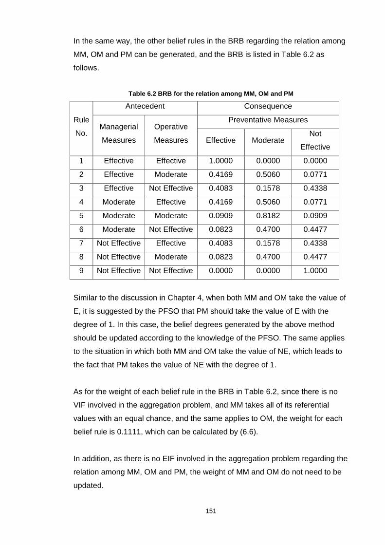
151
In the same way, the other belief rules in the BRB regarding the relation among
MM, OM and PM can be generated, and the BRB is listed in Table 6.2 as
follows.
Table 6.2 BRB for the relation among MM, OM and PM
Rule
No.
Antecedent Consequence
Managerial
Measures
Operative
Measures
Preventative Measures
Effective Moderate Not
Effective
1 Effective Effective 1.0000 0.0000 0.0000
2 Effective Moderate 0.4169 0.5060 0.0771
3 Effective Not Effective 0.4083 0.1578 0.4338
4 Moderate Effective 0.4169 0.5060 0.0771
5 Moderate Moderate 0.0909 0.8182 0.0909
6 Moderate Not Effective 0.0823 0.4700 0.4477
7 Not Effective Effective 0.4083 0.1578 0.4338
8 Not Effective Moderate 0.0823 0.4700 0.4477
9 Not Effective Not Effective 0.0000 0.0000 1.0000
Similar to the discussion in Chapter 4, when both MM and OM take the value of
E, it is suggested by the PFSO that PM should take the value of E with the
degree of 1. In this case, the belief degrees generated by the above method
should be updated according to the knowledge of the PFSO. The same applies
to the situation in which both MM and OM take the value of NE, which leads to
the fact that PM takes the value of NE with the degree of 1.
As for the weight of each belief rule in the BRB in Table 6.2, since there is no
VIF involved in the aggregation problem, and MM takes all of its referential
values with an equal chance, and the same applies to OM, the weight for each
belief rule is 0.1111, which can be calculated by (6.6).
In addition, as there is no EIF involved in the aggregation problem regarding the
relation among MM, OM and PM, the weight of MM and OM do not need to be
updated.
152
If for a certain port, MM is assessed as (E, 0.4576), (M, 0.2599), (NE, 0.2825)
while OM is assessed as (E, 0.1327), (M, 0.2442), (NE, 0.6232), as there is no
BF involved in the aggregation problem, the belief degrees assigned to the
referential values of MM and OM don’t need to be updated. Therefore, PM can
be generated as (Effective, 0.4764), (M, 0.2673), (NE, 0.2563) by RIMER as
introduced in Chapter 2.
As discussed in Section 6.5.1, the 36 BRBs in Appendix 5 are all generated
based on the assumption that the information of antecedents in the BRBs
should be aggregated heterogeneously. However, besides the BRB describing
the relation among MM, OM and PM, among the 36 BRBs in Appendix 5, there
are other BRBs in which the information of the antecedents should be
aggregated homogeneously. Therefore, the belief degrees in those BRBs
should be modified, and the modified BRBs are listed in Appendix 7.
6.4.3 Information aggregation with EIF(s) involved
In the aggregation pattern with EIF(s), one of the key problems is how to set an
appropriate threshold for the factor which is an EIF of the other factors. Usually,
such a threshold indicates an unacceptable low performance or a dominant high
performance of the factor.
If there exist some regulations relevant to the factor, the threshold can be
specified according to the regulations. For example, among the factors of
Response Activity (RA), Development of Contingency Plan (DCP), Update of
Contingency Plan (UCP) and Drill of Contingency Plan (DRCP), all parent
factors (DCP, UCP and DRCP) are “a kind of” child factor (RA), and if
contingency plans are not updated or drilled above a certain frequency, the
influence of DCP on RA will be restricted. Therefore, both UCP and DRCP are
an EIF of DCP regarding RA. From our interview with PFSOs in the UK, it is
known that they are required to update and drill contingency plans at least once
every 3 years by TRANSEC. On the other hand, from Appendix 2, it is known
that, both UCP and DRCP can take 3 referential values : ‘Good’ (G), ‘Moderate’
(M) and ‘Poor’ (P), which has the meaning of “the update/drill is conducted once
153
every year”, “the update/drill is conducted once every 3 years” and “there is no
update/drill conducted for contingency plans” respectively. If the utility of the 3
referential values for both UCP and DRCP, i.e., G, M and P, are set as 1, 0.5
and 0, the threshold of UCP and DRCP should be set as 0.5, as it is required
that the update/drill should be conducted at least once every 3 years, when the
utility of UCP/DRCP is below 0.5, the minimum requirement on UCP/DRCP
cannot be satisfied, and thus the impact of DCP on RA will be restricted.
On the other hand, if there is no regulations explicitly regulate the information
regarding the factor, the threshold should be specified by subjective judgments
according to the preference of PFSOs and ports’ environment. For example, as
discussed in Section 6.2.2, among the factors of Intervention Measures (IM),
Preventative Measures (PM), Responsive Measures (RSM) and Recovery
Measures (RCM), PM is an EIF of both RSM and RCM. As there is no specific
regulation regarding the performance of preventative measures against cargo
theft in a port storage area, the threshold of PM should be specified by the
PFSO of the port according to his subjective judgment and the specific
environment of the port. If the cargo listed in the International Maritime
Dangerous Goods Code (IMDG Code) is stored in the port and there are critical
infrastructures nearby, the threshold of PM will be relatively high, as the
consequence of cargo theft on the IMDG code is catastrophic if it cannot be
prevented. In addition, if the PFSO is risk-averse, i.e., he always prefer to
developing high-standard measures to prevent cargo theft from happening
instead of responding to and recovery from the situation after cargo theft
already happens, the threshold of PM will also be relatively high, as the PFSO
cannot accept a relatively low standard of preventative measures.
In summary, to specify a threshold of a certain factor which is the EIF of other
factors regarding cargo theft in a port storage area along a CLSC, there needs
a comprehensive consideration of regulations relevant to the factor (if any),
referential values of the factor, meaning and utility of the referential values,
preference of PFSOs, environment of ports, etc.
154
As an example for information aggregation with existence of EIF, the factors of
Hardware Feature (HF), Software Feature (SF), and Facility Feature (FF) are
considered here. In a port storage area, hardware, including CCTV system,
access control system, alarm system, etc., is more critical in preventing cargo
theft than software, which only refers to information system running in the port.
Therefore, if the performance of HF is below a threshold, the impact of SF on
FF will be restricted, i.e., HF is an N-EIF of SF regarding FF. According to the
preference of PFSO, the threshold of HF, HFt , is set to be 0.6, which means that
if the utility of HF is less than 0.6, the effect of SF on FF will be influenced. On
the other hand, according to real data collected from a port in China, HF of the
port can be represented by (Good, 0.0871), (Moderate, 0.4238), (Poor,
0.4891), therefore, if the utility of ‘Good’, ‘Moderate’ and ‘Poor’ are assumed to
be 1, 0.5 and 0 respectively, the utility of HF in the port, ( )U HF , is 0.2990.
Since ( ) HFU HF t< , the weight of each parent factor in the information
aggregation model, i.e., the weight of each antecedent in the corresponding
BRB should be updated.
As HF plays a more critical role in maintaining security against cargo theft in a
port storage area than SF does, the initial weight of the 2 antecedents are
0.8HFδ = and 0.2SFδ = , respectively. According to the fact that HF is an N-EIF of
SF, and 0.6HFt = , ( ) 0.2990U HF = , SFδ can be updated according to (6.2) as
follows:
( )min 1, 0.0997SF SF
HF
U HF
tδ δ
′ = =
As 0.8HF HFδ δ′ = = , the updated weight for HF and SF after normalization are:
0.8892HFδ = and 0.1108SFδ = .
Further, as in general, the probability that HF takes any of its referential value is
not influenced by SF and vice versa, there is no VIF existing in the information
aggregation process. If both HF and SF have the same probabilities to take
their referential values, according to (6.6), the weight of each rule in the
corresponding BRB is 0.1667. In addition, for a certain security assessment, as
155
the extent to which HF takes any of its referential value is not influenced by SF
and vice versa, there is no BF involved in the information aggregation process,
accordingly, there is no need to update the belief distributions describing the
performance of HF and SF. Since HF, SF and FF have the same nature, the
corresponding BRB should be generated in a homogeneous way.
Therefore, based on BRB 8 in Appendix 7, if HF is (Good, 0.0871), (Moderate,
0.4238), (Poor, 0.4891) and SF is (Good, 0), (Poor, 1) according to the real
situation of the port, FF can be generated as (Good, 0.0525), (Moderate,
0.2104), (Poor, 0.7371) by the inference scheme of RIMER.
6.4.4 Information aggregation with VIF(s) involved
According to the discussion in Section 6.4.2.2, if 1 2, ,...,ii i iVA A A are VIF(s) of iA ,
the impact of 1 2, ,...,ii i iVA A A on iA is reflected by the conditional probability
( )1 2| , ,...,ii i i iVP A A A A , based on which, the weight of each belief rule in the
corresponding BRB is specified. Therefore, in information aggregation with
VIF(s), one of key problems is how to specify such conditional probabilities in a
rational way to reflect the impact of VIF on the aggregation process.
Normally, subjective judgments play an important role in the specification of the
conditional probabilities. For example, as discussed in Section 6.2.2, among the
factors of Physical Feature (PF), Historical Feature (HF), Employee Feature (EF)
and Facility Feature (FF), HF is a VIF for both EF and FF. According to
Appendix 2 and Appendix 3, HF and FF can take the referential values of ‘Good’
(G), ‘Moderate’ (M) and ‘Poor’ (P), while EF can take the value of ‘Good’ (G)
and ‘Poor’ (P). If according to the real situation of the port and the PFSO’s
judgment, there is no obvious improvement of the capability of security related
hardware and software in the port in history, and there is no obvious
improvement of the security awareness of people working in the port in history,
HF will have an obvious impact on current FF and current EF. Take EF as an
example, if HF is ‘Poor’, EF is more likely to be ‘Poor’ than to be ‘Good’, while if
HF is ’Good’, EF is more likely to be ‘Good’ than ‘Poor’. Therefore, the
conditional probabilities regarding the impact of HF on EF may be set as:
156
( ) 0.8P EF G HF G= = = , ( ) 0.2P EF P HF G= = =
( ) 0.5P EF G HF M= = = , ( ) 0.5P EF P HF M= = =
( ) 0.2P EF G HF P= = = , ( ) 0.8P EF P HF P= = =
On the other hand, if the capability of security related hardware or software has
been improved recently, or if the PFSO thinks the security awareness of people
working in the port has been improved a lot, the impact of HF on FF or EF will
be trivial. In this case, the conditional probabilities regarding the impact of HF
on EF may be set as:
( ) 0.6P EF G HF G= = = , ( ) 0.4P EF P HF G= = =
( ) 0.5P EF G HF M= = = , ( ) 0.5P EF P HF M= = =
( ) 0.4P EF G HF P= = = , ( ) 0.6P EF P HF P= = =
Note that, the impact of HF on FF can be set similarly.
As an example to illustrate information aggregation with VIF involved, the
factors of PF, HF, FF and EF are considered here. According to real situation in
a port, there is no obvious improvement of the capability of security related
hardware/software or the security awareness of people in the port, thus, as
discussed above, the impact of HF when it takes the referential value G on FF
and EF can be specified as:
( ) 0.8P EF G HF G= = = , ( ) 0.2P EF P HF G= = =
( ) 0.7P FF G HF G= = = , ( ) 0.2P FF M HF G= = = , ( ) 0.1P FF P HF G= = =
In addition, if it is assumed that ( ) ( ) ( ) 1/3P HF G P HF M P HF P= = = = = = ,
according to (6.6), we have:
( )( ) ( ) ( )
, ,
0.1867
P HF G EF G FF G
P HF G P EF G HF G P FF G HF G
= = = =
= = = = = =

157
Correspondently, the weight of the belief rule with the packet antecedent
“Historical Feature is Good AND Employee Feature is Good AND Facility
Feature is Good” is 0.1867. Similarly, the weight of the other belief rules in the
BRB can be specified.
In addition, among HF, EF and FF, as FF plays a key role in maintaining
security of a port, the weight of FF is assigned as 0.7FFδ = , while
0.15EF FFδ δ= = . Further, among HF, EF and FF, the low/high performance of
any factor can be compensated/offset by other factors, therefore, there is no
EIF involved in the aggregation process, and there is no need to update the
weight of HF, EF and FF. Moreover, for HF, EF and FF, when a certain security
assessment is conducted, the extent to which any factor taking its referential
value is not dependent on referential value taken by other factors, there is no
BF involved in the aggregation process, which makes it unnecessary to update
the belief distributions describing HF, EF and FF. Since HF, EF and FF have
the same nature as PF, the BRB regarding the relationship among them should
be generated in a homogeneous way, and the BRB is listed as BRB 6 in
Appendix 7.
According to the real situation of a port in China, HF is (Good, 0), (Moderate, 1),
(Poor, 0), EF is (Good, 1), (Poor, 0) and FF is (Good, 0.7028), (Moderate,
0.2223), (Poor, 0.0748), based on BRB 6 in Appendix 7, PF can be generated
as (Good, 0.4440), (Moderate, 0.3895), (Poor, 0.1665) by the inference
scheme of RIMER, as introduced in Chapter 2.
6.4.5 Information aggregation with the coexistence of EIF and BF
In the security assessment model in Appendix 1, one of the basic units for
information aggregation contains the factor of Response Activity (RA),
Development of Contingency Plan (DCP), Update of Contingency Plan (UCP)
and Drill of Contingency Plan (DRCP), with RA being a child factor and DCP,
UCP, DRCP being parent factors. Since both the update and the drilling of
contingency plans can only be applied to existing contingency plans, therefore,
the extents to which UCP and DRCP can take their referential values for a
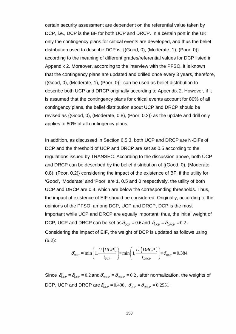
158
certain security assessment are dependent on the referential value taken by
DCP, i.e., DCP is the BF for both UCP and DRCP. In a certain port in the UK,
only the contingency plans for critical events are developed, and thus the belief
distribution used to describe DCP is: (Good, 0), (Moderate, 1), (Poor, 0)
according to the meaning of different grades/referential values for DCP listed in
Appendix 2. Moreover, according to the interview with the PFSO, it is known
that the contingency plans are updated and drilled once every 3 years, therefore,
(Good, 0), (Moderate, 1), (Poor, 0) can be used as belief distribution to
describe both UCP and DRCP originally according to Appendix 2. However, if it
is assumed that the contingency plans for critical events account for 80% of all
contingency plans, the belief distribution about UCP and DRCP should be
revised as (Good, 0), (Moderate, 0.8), (Poor, 0.2) as the update and drill only
applies to 80% of all contingency plans.
In addition, as discussed in Section 6.5.3, both UCP and DRCP are N-EIFs of
DCP and the threshold of UCP and DRCP are set as 0.5 according to the
regulations issued by TRANSEC. According to the discussion above, both UCP
and DRCP can be described by the belief distribution of (Good, 0), (Moderate,
0.8), (Poor, 0.2) considering the impact of the existence of BF, if the utility for
‘Good’, ‘Moderate’ and ‘Poor’ are 1, 0.5 and 0 respectively, the utility of both
UCP and DRCP are 0.4, which are below the corresponding thresholds. Thus,
the impact of existence of EIF should be considered. Originally, according to the
opinions of the PFSO, among DCP, UCP and DRCP, DCP is the most
important while UCP and DRCP are equally important, thus, the initial weight of
DCP, UCP and DRCP can be set as 0.6DCPδ = and 0.2UCP DRCPδ δ= = .
Considering the impact of EIF, the weight of DCP is updated as follows using
(6.2):
( ) ( )min 1, min 1, 0.384DCP DCP
UCP DRCP
U UCP U DRCP
t tδ δ
′ = × × =
Since 0.2UCP UCPδ δ′ = = and 0.2DRCP DRCPδ δ′ = = , after normalization, the weights of
DCP, UCP and DRCP are 0.490DCPδ = , 0.2551UCP DRCPδ δ= = .

159
Furthermore, among DCP, UCP and DRCP, the probability of one factor taking
any of its referential values are not influenced by other factors, there is no VIF
involved in the aggregation process. According to Appendix 2, DCP, UCP and
DRCP have 3 referential values, if it is assumed that in general, the referential
value of each factor has an equal probability to be taken, the weights of each
belief rule in the corresponding BRB are the same, i.e., 0.037, which is
calculated by (6.6).
As for the belief degrees in the corresponding BRB, since DCP, UCP and
DRCP are all ‘a kind of’ RA, the belief degrees should be generated based on
the fact that the information of DCP, UCP and DRCP should be aggregated
homogeneously. The corresponding belief degrees are listed in BRB 14 in
Appendix 7.
In summary, for the basic information aggregation unit regarding the relation
among RA, DCP, UCP and DRCP, the following conclusions can be made:
considering the impact of BF, belief distribution of both UCP and DRCP should
be updated from (Good, 0), (Moderate, 1), (Poor, 0) to (Good, 0), (Moderate,
0.8), (Poor, 0.2); considering the impact of EIF, the weight of DCP, UCP and
DRCP are updated from 0.6, 0.2, 0.2 to 0.490, 0.2551, 0.2551, respectively; the
weight of each rule in the BRB is 0.037; and the belief degrees in the BRB are
listed in BRB 14 in Appendix 7. Therefore, according to the inference scheme of
RIMER, RA can be generated as (Effective, 0.1521), (Moderate, 0.5946), (Not
Effective, 0.2533).
6.4.6 Assessment of security against cargo theft in port storage area based on real data collected
In Chapter 4, data collected from 5 ports in both China and the UK are used to
validate the security assessment model developed, however, the information of
different factors are aggregated in the same way, i.e., heterogeneous
information aggregation without EIF(s), VIF(s) or BF(s). According to different
information aggregation patterns identified in this chapter, security level of the
same set of ports is assessed again based on the same set of data, with
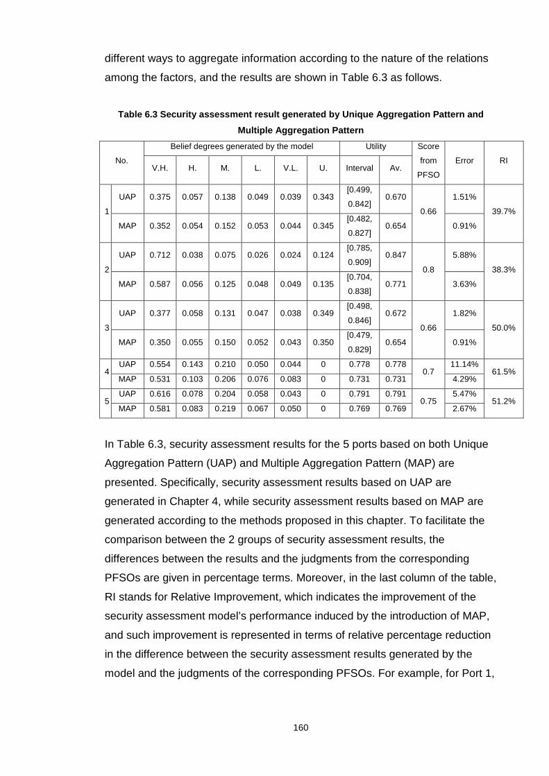
160
different ways to aggregate information according to the nature of the relations
among the factors, and the results are shown in Table 6.3 as follows.
Table 6.3 Security assessment result generated by U nique Aggregation Pattern and
Multiple Aggregation Pattern
No.
Belief degrees generated by the model Utility Score
from
PFSO
Error RI V.H. H. M. L. V.L. U. Interval Av.
1
UAP 0.375 0.057 0.138 0.049 0.039 0.343 [0.499,
0.842] 0.670
0.66
1.51%
39.7%
MAP 0.352 0.054 0.152 0.053 0.044 0.345 [0.482,
0.827] 0.654 0.91%
2
UAP 0.712 0.038 0.075 0.026 0.024 0.124 [0.785,
0.909] 0.847
0.8
5.88%
38.3%
MAP 0.587 0.056 0.125 0.048 0.049 0.135 [0.704,
0.838] 0.771 3.63%
3
UAP 0.377 0.058 0.131 0.047 0.038 0.349 [0.498,
0.846] 0.672
0.66
1.82%
50.0%
MAP 0.350 0.055 0.150 0.052 0.043 0.350 [0.479,
0.829] 0.654 0.91%
4 UAP 0.554 0.143 0.210 0.050 0.044 0 0.778 0.778
0.7 11.14%
61.5% MAP 0.531 0.103 0.206 0.076 0.083 0 0.731 0.731 4.29%
5 UAP 0.616 0.078 0.204 0.058 0.043 0 0.791 0.791
0.75 5.47%
51.2% MAP 0.581 0.083 0.219 0.067 0.050 0 0.769 0.769 2.67%
In Table 6.3, security assessment results for the 5 ports based on both Unique
Aggregation Pattern (UAP) and Multiple Aggregation Pattern (MAP) are
presented. Specifically, security assessment results based on UAP are
generated in Chapter 4, while security assessment results based on MAP are
generated according to the methods proposed in this chapter. To facilitate the
comparison between the 2 groups of security assessment results, the
differences between the results and the judgments from the corresponding
PFSOs are given in percentage terms. Moreover, in the last column of the table,
RI stands for Relative Improvement, which indicates the improvement of the
security assessment model’s performance induced by the introduction of MAP,
and such improvement is represented in terms of relative percentage reduction
in the difference between the security assessment results generated by the
model and the judgments of the corresponding PFSOs. For example, for Port 1,

161
under UAP, the difference between the security assessment result generated by
the model and the judgment of the PFSO is 1.51%, after the introduction of
MAP, the difference reduces to 0.91%, and thus the Relative Improvement can
be calculated as:
(1.51%-0.91%)/1.51%=39.7%.
From Table 6.2, it can be seen that after the introduction of MAP, the
performance of the security assessment model is improved, which reflects the
necessity and rationality of the introduction of MAP.
In addition to security assessment of a port storage area against cargo theft, the
concept of aggregating information in different patterns and the methods to
handle different information aggregation patterns can also be applied for
security assessment of other organizations involved in a CLSC against different
threats, and for security assessment of the whole organizations involved in a
CLSC. Especially, since the interactions among different factors with
information to be aggregated can be reflected by the introduction of EIF, VIF
and BF, the concept and the methods proposed in this chapter can be applied
for security assessment of a whole CLSC by taking interactions among different
organizations in the CLSC into consideration. One of the typical examples
regarding the capability of the different aggregation patterns in representing
interactions among different organizations along a CLSC can be reflected by
the following fact: along a CLSC, if the security level of a certain organization is
below a certain threshold, the security of the whole CLSC will not be high, as
the CLSC is the most vulnerable at that organization. In this case, the low
performance of the organization with security level below a threshold cannot be
compensated by high performance of other organizations in the CLSC, thus, the
organization is an N-EIF of other organizations when the security level of each
organization along the CLSC is aggregated to form the overall security level of
the whole CLSC.
6.5 Conclusion
162
Driven by the fact that the relations among factors in the security assessment
model in Appendix 1 may be inherently different, this chapter proposes the
concept that the information of the factors in different basic information
aggregation units should be aggregated in different patterns according to the
nature of relations among the factors.
There are 3 major contributions of this chapter which are summarized as follows.
1) By investigating the nature of relations among different factors in the security
assessment model in Appendix 1, different information aggregation patterns are
proposed accordingly to make the security assessment process more
reasonable and the assessment result more realistic, this contribution is vital as
currently most information aggregation methods only consider a single fixed
information aggregation pattern despite of the fact that the nature of relations
among different factors may be various in CLSC security assessment models. 2)
A set of novel methods are proposed to handle different aggregation patterns
existing in the security assessment model in Appendix 1 based on RIMER, due
to its advantages over other existing methods for information aggregation, as
summarized at the end of Section 6.3, and according to the characteristics of
CLSC operation, all the advantages of RIMER are essential for CLSC security
assessment. 3) From a more general view, the aggregation patterns identified in
this chapter reflect the interaction among the factors with information to be
aggregated by the introduction of EIF, VIF and BF. This character is crucial in
security assessment for a whole CLSC, as in CLSC operation, there are
inevitable interactions among different organizations involved in CLSC, and the
concept in this chapter provides an alternative to model such interactions.
To validate the aggregation patterns proposed in this chapter together with the
corresponding methods to handle the patterns, a set of case studies are
conducted based on real data collected from different ports in both China and
the UK. Compared to the security assessment results generated in Chapter 4,
the results based on different aggregation patterns proposed in this chapter are
closer to PFSO’s judgments, which verifies the necessity and rationality of the
contributions of this chapter.

163
In addition, CLSC security assessment is in essence an MCDA problem. As
information aggregation is one of the major stages for MCDA (Marichal, 1998),
and many real MCDA problems are so complex that it is unlikely the features of
relations among different criteria are the same, the concept that the information
should be aggregated in different patterns according to the features of relations
among criteria have great potential to be applied in many other complex MCDA
problems apart from CLSC security assessment.

164
7 Chapter 7 Handling Different Kinds of Incomplete In formation for Security Assessment of CLSC
Abstract
From the discussion in previous chapters, it is clear that incompleteness is
prevalent in CLSC security assessment. In this chapter, the incompleteness
existing in the security assessment model discussed in previous chapters is
categorized and analyzed in detail. According to the characteristics of different
kinds of incompleteness, the limitations of RIMER in handling incomplete
information are revealed, and a set of new models based on RIMER are
proposed to overcome the limitations identified. To validate the methods, a set
of case studies are conducted according to the data collected from the ports in
both China and the UK, and the results generated from the case studies are
compared with the results generated in case studies in previous chapters.
7.1 Introduction
Due to the complexity of CLSC operation, it is unlikely that all the information
required by the security assessment model discussed in Chapter 3 and Chapter
4 is always available. For example, in the case studies in Chapter 4 and
Chapter 6, only 2 out of 5 ports have all the information required. Therefore,
how to conduct security assessment without full information or how to handle
incomplete information in security assessment process is one of the key
questions to be answered to ensure the rationality and practicability of the
security assessment model.
Facing this situation, in this chapter, the incompleteness existing in the security
assessment model discussed in previous chapters is investigated in detail.
According to the investigation, the incompleteness is divided into different
categories, and the limitations of RIMER in handling different kinds of
incompleteness are then revealed. To overcome the limitations, a set of new
models are proposed and the models are validated through case studies
conducted at the end of the chapter.

165
7.2 Different sources of incompleteness and differe nt categories of incompleteness
For some practical problems under complex environment, it is usually difficult, if
not impossible, to get complete information to describe the problems. For
example, for CLSC security assessment, the incompleteness of information
may be caused by the followings reasons:
• The information is not available. For example, to assess the performance
of an alarm system in a certain port along a CLSC, the information about
the robustness of the alarm system should be collected. However, at the
time when security assessment was conducted, the alarm system was
just updated for a month. As the robustness of the updated system
should only be fully revealed after it runs for a certain period of time, the
information on its robustness was not completely available when security
assessment was conducted.
• The information is available, but the cost to collect the information
compared to the benefit generated is too high. For example, currently,
access points are mainly controlled by 3 means in general, i.e.,
traditional lock/key, electronic key-card and biometric information. To
investigate the capability of access control system of a port storage area
along a CLSC, the information on how the access points of the port
storage area are controlled, and what is the percentage of different
means used to control the access points should be collected. However,
for a certain port, according to the PFSO’s knowledge, he only knew that
there is no access point of the port storage area controlled by biometric
information, and he is not sure how many access points are controlled by
traditional lock/key and electronic key-card respectively. In this case, if a
thorough investigation is conducted, the complete information on how the
access points are controlled will become available. However, the cost of
the investigation is very high relative to the benefit which can be
generated from the investigation, and thus, the information for the
capability of the access control system of the port storage area is
incomplete.
166
• The information is available, but it is too sensitive to be released. For
example, for some ports within a CLSC, some information, especially the
information on emergency response, is very sensitive, and thus it is not
accessible to public.
Note that, the incomplete information mentioned above is all about the input, or
the basic factors, of the security assessment model in Appendix 1, i.e., the
incompleteness is about the information for antecedents of BRBs under the
context of RIMER. Apart from the incompleteness in antecedents,
incompleteness may also exist in the knowledge about the relation among
antecedents and consequence in a BRB when security assessment is
conducted. The incompleteness in the knowledge may be caused by the fact
that the expert is incapable of providing complete information due to the
complexity of the problem, or the fact that a group of experts cannot reach an
agreement on the relation between the packet antecedent and the consequence.
To facilitate the following analysis, Figure 4.1 is selected as a basis for the
discussion in this chapter. According to the discussion in previous chapters,
Figure 4.1 is corresponding to a BRB with the kth rule represented by (4.2). In
addition, in Figure 4.1, the input information about the antecedent
( )1,2,...,iA i M∈ can be represented by (4.24), in which, if
1
1i
i
i
M
ipp
α=
<∑ , the input
information is said to be incomplete, and the extent of incompleteness is
represented by 1
1i
i
i
M
ipp
α=
−∑ . Moreover, for the kth rule in the BRB corresponding
to Figure 4.1 as represented by (4.2), if 1
1N
iki
β=
<∑ , it can be said that the
information about relation among the antecedents and the consequence in the
rule is incomplete, and the extent of incompleteness is represented by1
1N
iki
β=
−∑ .
167
According to different ways to assign1
1i
i
i
M
ipp
α=
−∑ or1
1N
iki
β=
−∑ , the incompleteness
can be categorized as local incompleteness and global incompleteness (Xu, et
al., 2006):
• If for antecedent iA , the information of which is represented by (4.24),
1
1i
i
i
M
ipp
α=
−∑ is assigned to the whole set of 1 2, ,...,ii i iMA A A , i.e.,
1
1i
i
i
M
ipp
α=
−∑
can be assigned to any individual referential value ( )1,2,...,iip i iA p M∈ ,
the incompleteness is referred to as global incompleteness;
• If 1
1i
i
i
M
ipp
α=
−∑ can only be assigned to a real subset of 1 2, ,...,ii i iMA A A , e.g.,
( ) 1, ...,i iiit isi tA A A+
with , 1,2,..., 1i i it s M∈ − , 1 i i it s M≤ < ≤ and
[ ] [ ], 1,i i it s M⊂ , i.e., 1
1i
i
i
M
ipp
α=
−∑ can only be assigned to the grade fromiitA
to ( )iis i iA s t≠ with the requirement that it and is cannot take the value of 1
and iM simultaneously, the incompleteness is referred to as local
incompleteness.
Similar result can be generated regarding1
1N
iki
β=
−∑ .
Note that, both categories of incompleteness exist in the security assessment
model in Appendix 1, e.g., the incompleteness in previous example regarding
robustness of alarm system is global incompleteness, since the degree of belief
unassigned to any referential values describing the robustness of the alarm
system due to incomplete information can be assigned to all the referential
values when more information is available. On the other hand, the
incompleteness in previous example regarding capability of access control
system is local incompleteness, since the degree of belief unassigned to any
referential values describing the capability of the access control system due to

168
incomplete information can only be assigned to some of certain referential
values when more information is available.
7.3 Limitations of RIMER in handling incomplete inf ormation
7.3.1 Current scheme to handle incompleteness in RI MER
Facing the prevalence of incompleteness in many complex applications, a
scheme was developed in (Yang, et al., 2006) to handle incomplete information
existing in the inference process under the framework of RIMER.
Specifically, in a BRB corresponding to Figure 4.1, if the information of one or
more antecedent(s) is incomplete, the belief degrees in the consequence of the
( )1,2,...,kth k L∈ rule kR in the BRB, as represented by ( )1,2,...,ik i Nβ = in (4.2),
should be updated by (7.1) as follows:
( )
( )1 1
1
,
,
t
t
t
MM
tpt p
ik ik M
t
t k
t k
τ αβ β
τ
= =
=
=
∑ ∑
∑ (7.1)
In (7.1), ( ) 1 if is used in defining , with 1,2,...,,
0 otherwiset kA R t M
t kτ=
=
, while
( )1,2,..., ; 1,2,...,ik i N k Lβ = = represents the degree to which the consequence D
can be described by its ith referential value in the kth rule before update, as
introduced in (4.2), ( )1,2,..., ; 1,2,...,ttp t tt M p Mα = = represents the degree to
which antecedent tA can be described by its tp th referential value, as introduced
by (4.24), and ikβ is the value of ikβ after update.
According to (7.1), 1
1N
iki
β=
−∑ can be used to reflect the extent of incompleteness
that exists in the input information regarding the antecedents of the BRB. For
example, if in Figure 4.1, the following conditions are satisfied: 1) 3M = , i.e.,
there are 3 antecedents ( 1 2 3, ,A A A ) influencing consequence D ; 2) all the
169
antecedents are used in defining all the belief rules in the BRB, i.e., ( ), 1t kτ = for
all 1,2,3t = and 1,2,...,k L= ; 3) the input information for both 1A and 3A is complete,
i.e., 1
1
1
11
1M
pp
α=
=∑ and
3
3
3
31
1M
pp
α=
=∑ ; 4) for 2A ,2
2
2
21
0.9M
pp
α=
=∑ , indicating that there is
incompleteness in the input information for 2A , then, the belief degrees in the
consequence of all belief rules in the BRB are updated as follows:
( )
( )( )
3
1 1
3
1
,2.9
0.9667 1,2,..., ; 1,2,...,3,
t
t
t
M
tpt p
ik ik ik ik
t
t k
i N k Lt k
τ αβ β β β
τ
= =
=
= = = = =
∑ ∑
∑ (7.2)
If originally, the information regarding the relation among 1 2 3, ,A A A and D is
complete, i.e., 1
1N
iki
β=
=∑ for all 1,2,...,k L= , after update, 1
09667N
iki
β=
=∑ for all
1,2,...,k L= according to (7.2), indicating the extent of incompleteness for each
rule in the BRB caused by incomplete input is 1
1 0.0333N
iki
β=
− =∑ . From the
example, it can be seen that the incompleteness in the input information for 2A
is reflected by the incompleteness existing in all belief rules in the BRB, i.e., the
incompleteness in the knowledge contained in the BRB regarding the relation
among 1 2 3, ,A A A and D in all belief rules.
Alternatively, in the above example, it is also possible that the input information
regarding all the antecedents of the BRB is complete, which leads to
ik ikβ β= according to (7.1) for all 1,2,..., ; 1,2,...,i N k L= = , while the information
regarding the relation among 1 2 3, ,A A A and D in all belief rules is incomplete,
which leads to1
1N
iki
β=
<∑ for all 1,2,...,k L= . In this case,1 1
1N N
ik iki i
β β= =
= <∑ ∑ , and
1
1N
iki
β=
−∑ can be used to represent the extent of incompleteness incurred when
the belief rules in the BRB are established, i.e., the extent of incompleteness

170
regarding the knowledge on the relation among antecedents and consequence
in the BRB.
In the above 2 examples, both the incompleteness about input information of
the BRB and the incompleteness about the knowledge on the relation among
the antecedents and consequence of the BRB are reflected by1
1N
iki
β=
−∑ , in other
words, the 2 kinds of incompleteness cannot be differentiated in the above
examples.
7.3.2 Limitations of RIMER in handling incompletene ss
Handling incompleteness through the process introduced above have some
limitations, which are analyzed as follows.
Firstly, according to the way to represent incompleteness, local incompleteness
and global incompleteness cannot be differentiated: the incompleteness of the
input information regarding antecedent ( )1,2,...,iA i M∈ in Figure 4.1 is
uniformly represented by1
1 0i
i
i
M
ipp
α=
− >∑ , while the incompleteness of the
knowledge regarding the relation among ( )1,2,...,iA i M= and D in Figure 4.1 is
uniformly represented by 1
1N
iki
β=
−∑ . There is no discussion on how to allocate
1
1i
i
i
M
ipp
α=
−∑ and1
1N
iki
β=
−∑ among relevant referential values.
Secondly, according to the process to handle incompleteness in RIMER, it can
be seen that the incompleteness in input information of the antecedents of a
BRB and the incompleteness in the knowledge regarding relation among
antecedents and consequence of the BRB cannot be differentiated, as in
current scheme, the incompleteness in input information is transformed into the
incompleteness in the knowledge by the above process. However, as the two
kinds of incompleteness have completely different sources and different
171
inherent features, such a transformation without assumption and explanation is
not appropriate.
In addition, in some extreme cases, incompleteness cannot be handled by
current RIMER. For example, among the antecedents of 1 2, ,..., MA A A in Figure
4.1, if there is no information about one of the antecedents, e.g.,
( )1,2,...,iA i M∈ , i.e., 0ijα = for all 1,2,..., ij M= , according to the inference
scheme of RIMER introduced in Chapter 2, i
kipα in (4.26) will be 0, since
, 1,2,...,i
kip ij ij Mα α∈ = . Further, when 0
i
kipα = , the total match degree between
the input and the packet antecedent in the kth rule, kα , will be 0 according to
(4.26). If in the BRB corresponding to Figure 4.1, iA is used to define all the
belief rules, for all 1,2,...,k L= , 0kα = , which will make it infeasible to calculate
activation weight of each belief rule in the BRB using (4.28), and thus, the
inference cannot be conducted according to current inference scheme of
RIMER. Therefore, for current RIMER, if there is no information about one or
more antecedents of the BRB, the inference cannot be conducted.
To overcome the limitations mentioned above, an improved process to handle
incompleteness under the framework of RIMER is proposed in the next section.
7.4 A new method to handle incompleteness based on RIMER
7.4.1 Representation of both local and global incom pleteness
As discussed in Section 7.2, the incompleteness can be categorized as local
incompleteness and global incompleteness, and the difference between them is
reflected by the way to assign the degree of belief which has not been assigned
to any individual referential values.
As the information about an antecedent ( )1,2,...,iA i M∈ in Figure 4.1 is
represented by a belief distribution as indicated in (4.24), if the information is
incomplete, and the incompleteness is global, 1
1i
i
i
M
ipp
α=
−∑ can be assigned to any
172
individual referential values from 1iA toiiMA . Accordingly, the belief assigned to
any referential value ( )1,2,...,iip i iA p M∈ can be considered as an interval with
the lower boundary ofiipα and the upper boundary of
1
1i
i i
i
M
ip ipp
α α=
+ − ∑ . Similarly,
if the incompleteness is local, 1
1i
i
i
M
ipp
α=
−∑ can be only assigned to the referential
values fromiitA to
iisA as discussed in Section 7.2, and the belief degree assigned
to the referential value ofiiqA with , 1,...,i i i iq t t s∈ + can be considered as an
interval 1
, 1i
i i i
i
M
iq iq ipp
α α α=
+ −
∑ , while the belief degree assigned to the grade of
iirA with 1,2,..., 1 1, 2,...,i i i i ir t s s M∈ − + +∪
remains
iirα , which can also be
considered as a special interval with both lower boundary and upper boundary
being the value ofiirα . Note that, for both complete and incomplete information
regarding ( )1,2,...,iA i M= , if belief degrees are represented by intervals, the
sum of belief degrees assigned to all referential values of iA is required to be 1.
Corresponding to the incompleteness of input information for antecedents,
similar conclusions can also be drawn regarding the incompleteness of the
knowledge about the relation among antecedents and consequences in a BRB.
Therefore, to accommodate both global and local incompleteness under the
same framework, belief degrees in (4.24) and (4.2) are represented in the form
of intervals instead of precise values. Accordingly, the information of the ith
antecedent in Figure 4.1, iA , can be represented by (7.3) based on (4.24) as
follows, with iip Lα
and iip Uα being lower and upper bound of
iipα :
( ) ( ) , ; 1,2,..., , 1,2,...,i ii ip ip i iS A A p M i Mα= = = , with ,
i i iip ip L ip Uα α α ∈ and
1
1i
i
i
M
ipp
α=
=∑ (7.3)
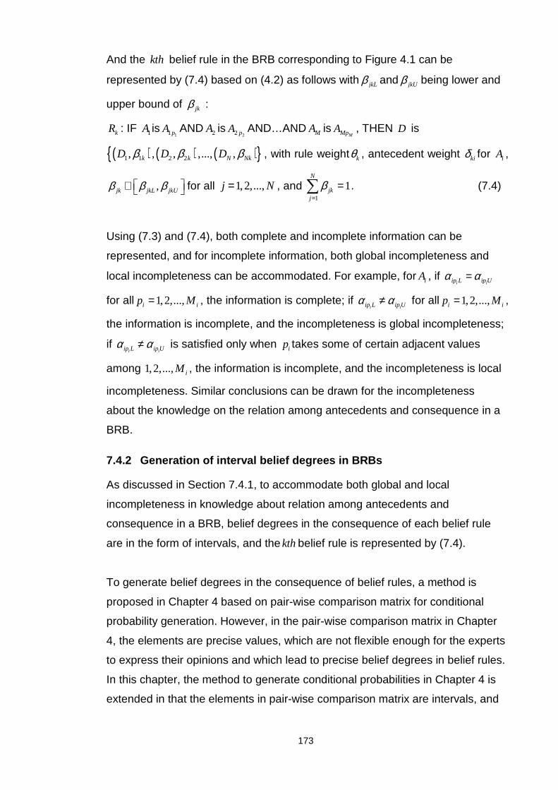
173
And the kth belief rule in the BRB corresponding to Figure 4.1 can be
represented by (7.4) based on (4.2) as follows with jkLβ and jkUβ being lower and
upper bound of jkβ :
kR : IF 1A is11pA AND 2A is
22 pA AND…AND MA isMMpA , THEN D is
( ) ( ) ( ) 1 1 2 2, , , ,..., ,k k N NkD D Dβ β β , with rule weight kθ , antecedent weight kiδ for iA ,
,jk jkL jkUβ β β ∈ for all 1,2,...,j N= , and 1
1N
jkj
β=
=∑ . (7.4)
Using (7.3) and (7.4), both complete and incomplete information can be
represented, and for incomplete information, both global incompleteness and
local incompleteness can be accommodated. For example, for iA , if i iip L ip Uα α=
for all 1,2,...,i ip M= , the information is complete; if i iip L ip Uα α≠ for all 1,2,...,i ip M= ,
the information is incomplete, and the incompleteness is global incompleteness;
if i iip L ip Uα α≠ is satisfied only when ip takes some of certain adjacent values
among 1,2,..., iM , the information is incomplete, and the incompleteness is local
incompleteness. Similar conclusions can be drawn for the incompleteness
about the knowledge on the relation among antecedents and consequence in a
BRB.
7.4.2 Generation of interval belief degrees in BRBs
As discussed in Section 7.4.1, to accommodate both global and local
incompleteness in knowledge about relation among antecedents and
consequence in a BRB, belief degrees in the consequence of each belief rule
are in the form of intervals, and the kth belief rule is represented by (7.4).
To generate belief degrees in the consequence of belief rules, a method is
proposed in Chapter 4 based on pair-wise comparison matrix for conditional
probability generation. However, in the pair-wise comparison matrix in Chapter
4, the elements are precise values, which are not flexible enough for the experts
to express their opinions and which lead to precise belief degrees in belief rules.
In this chapter, the method to generate conditional probabilities in Chapter 4 is
extended in that the elements in pair-wise comparison matrix are intervals, and
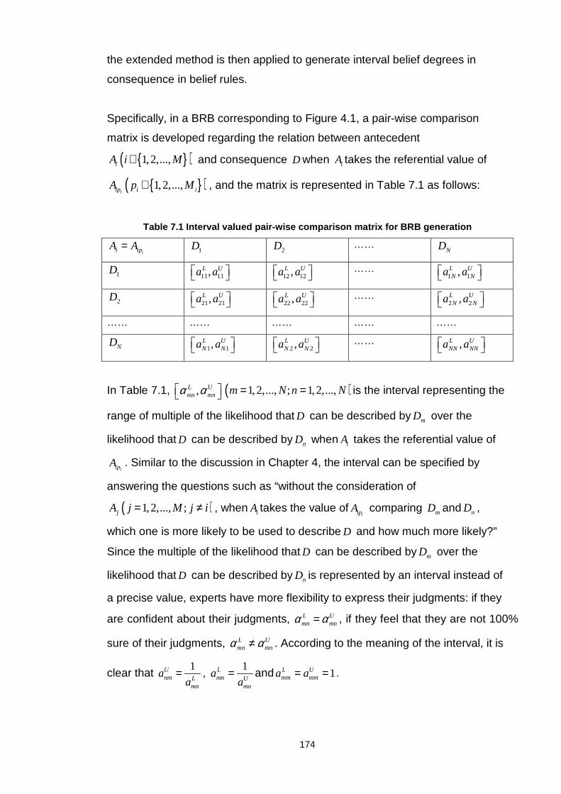
174
the extended method is then applied to generate interval belief degrees in
consequence in belief rules.
Specifically, in a BRB corresponding to Figure 4.1, a pair-wise comparison
matrix is developed regarding the relation between antecedent
( )1,2,...,iA i M∈ and consequence D when iA takes the referential value of
( )1,2,...,iip i iA p M∈ , and the matrix is represented in Table 7.1 as follows:
Table 7.1 Interval valued pair-wise comparison matr ix for BRB generation
ii ipA A= 1D 2D …… ND
1D 11 11,L Ua a 12 12,L Ua a ……
1 1,L UN Na a
2D 21 21,L Ua a 22 22,L Ua a ……
2 2,L UN Na a
…… …… …… …… ……
ND 1 1,L U
N Na a 2 2,L UN Na a …… ,L U
NN NNa a
In Table 7.1, ,L Umn mnα α ( )1,2,..., ; 1,2,...,m N n N= = is the interval representing the
range of multiple of the likelihood that D can be described by mD over the
likelihood that D can be described by nD when iA takes the referential value of
iipA . Similar to the discussion in Chapter 4, the interval can be specified by
answering the questions such as “without the consideration of
( )1,2,..., ;jA j M j i= ≠ , when iA takes the value ofiipA comparing mD and nD ,
which one is more likely to be used to describe D and how much more likely?”
Since the multiple of the likelihood that D can be described by mD over the
likelihood that D can be described by nD is represented by an interval instead of
a precise value, experts have more flexibility to express their judgments: if they
are confident about their judgments, L Umn mnα α= , if they feel that they are not 100%
sure of their judgments, L Umn mnα α≠ . According to the meaning of the interval, it is
clear that 1U
nm Lmn
aa
= , 1L
nm Umn
aa
= and 1L Umm mma a= = .

175
Based on the pair-wise comparison matrix with interval elements in Table 7.1,
the priority of each referential value used to describe D can be generated. In
(Wang, et al., 2005), a method was proposed to derive priority based on interval
valued pair-wise comparison matrix, and the method, which is briefly introduced
as follows, is applied in this chapter to derive the priority of referential values of
D .
As indicated by Wang, et al. (2005), before the priorities are generated, the
consistency of the interval valued pair-wise comparison matrix should be
checked. Specifically, the matrix ( )mn N NA a
×= ( )L U
mn mn mnaα α≤ ≤ in Table 7.1 is
consistent if and only if for all , , 1,2,...,m n k N= , ( ) ( )max minL L U Umk kn mk kn
kka a a a≤ .
If the matrix in Table 7.1 is consistent, the range of ip jω
( )1,2,..., , 1,2,...,i ip M j N∈ = , which is the priority of the referential value of jD
when iA takes the referential value of ( )1,2,..., , 1,2,...,iip i iA i M p M∈ ∈ , can be
generated by the following pair of linear programming model withip jω as decision
variables:
ip joptimize ω (7.5)
Subject to: SΩΩ∈ (7.6)
In (7.5), ‘optimizing the objective function’ refers to either maximizing or
minimizing the objective function (the same applies to the objective functions in
the optimization models in the rest of the thesis); in (7.6), ( )1 2, ,...,i i i
T
p p p Nω ω ωΩ = ,
and
( )1 21
, ,... , 1, 0, 1,2,..., , 1,2,...,i
i i i i i
i
Np mL U
p p p N mn mn p n p nnp n
S a a m N n Nω
ω ω ω ω ωωΩ
=
= Ω = ≤ ≤ = > = =
∑
Otherwise, if the matrix is inconsistent, the following pair of non-linear
programming model can be applied to derive the range ofip jω :

176
optimize ip jω (7.7)
Subject to: ( ) ( )1
1 1
ˆ1 1 0, 1,2,...,ˆ
i
i i
j Np k
p j jk p kk k jjk
N RI CR a j Na
ωω ω
−
= = +
− − + ⋅ + = =∑ ∑ (7.8)
1
1i
N
p jj
ω=
=∑ (7.9)
ˆ , 1,2,..., 1; 1, 2,...,L Ujk jk jka a a j N k j j N≤ ≤ = − = + + (7.10)
CR δ≤ (7.11)
In (7.8), ˆ jka is an element in ( )ˆ ˆ jk N NA a
×= , a crisp comparison matrix randomly
generated from the interval comparison matrix ( )jk N NA a
×= in Table 7.1, with
ˆL Ujk jk jka a a≤ ≤ and ˆ ˆ1kj jka a= ; CR and RI are the Consistency Ratio and Random
Index of A , respectively, as discussed in Chapter 4; (7.9) is used to ensure the
sum of the priorities is 1 while (7.10) is used to restrict the range of ˆ jka in (7.8);
in (7.11), δ is the level of satisfactory consistency. In the model represented by
(7.7)-(7.11), the decision variables are:CR ,ip jω and ˆ jka .
The solutions of linear programming model (7.5)-(7.6) or non-linear
programming model (7.7)-(7.11) are represented byi
Lp jω and
i
Up jω , which are the
lower and upper boundary ofip jω , respectively. Since in both models, it is
required that 1
1i
N
p jj
ω=
=∑ , and both i
Lp jω and
i
Up jω are attainable, according to the
definition in Wang and Elhag (2006), ,i i
L Up j p jω ω ( )1,2,...,j N= are normalized.
Therefore, the interval of ,i i
L Up j p jω ω ( )1,2,...,j N= can be considered as the
range of the probability that D can be described by the referential value of jD on
the condition that iA takes the referential value of iipA in Figure 4.1, i.e.,
( ) ,i i i i
L Up j j i ip p j p jP D D A Aω ω ω = = = ∈ (7.12)
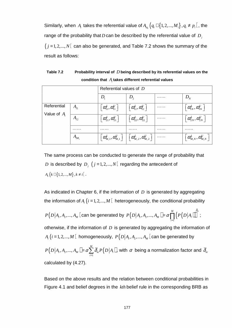
177
Similarly, when iA takes the referential value of ( )1,2,..., ,iiq i i i iA q M q p∈ ≠ , the
range of the probability that D can be described by the referential value of jD
( )1,2,...,j N= can also be generated, and Table 7.2 shows the summary of the
result as follows:
Table 7.2 Probability interval of D being described by its referential values on the
condition that iA takes different referential values
Referential values of D
1D 2D …… ND
Referential
Value of iA 1iA
11 11,L Uω ω 12 12,L Uω ω …… 1 1,L U
N Nω ω
2iA 21 21,L Uω ω 22 22,L Uω ω ……
2 2,L UN Nω ω
…… …… …… …… ……
iiMA 1 1,
i i
L UM Mω ω 2 2,
i i
L UM Mω ω …… ,
i i
L UM N M Nω ω
The same process can be conducted to generate the range of probability that
D is described by jD ( )1,2,...,j N= regarding the antecedent of
( )1,2,..., ,kA k M k i∈ ≠ .
As indicated in Chapter 6, if the information of D is generated by aggregating
the information of iA ( )1,2,...,i M= heterogeneously, the conditional probability
( )1 2, ,..., MP D A A A can be generated by ( ) ( )( )1 21
, ,...,kiM
M ii
P D A A A P D Aδ
α=
= ∏ ;
otherwise, if the information of D is generated by aggregating the information of
iA ( )1,2,...,i M= homogeneously, ( )1 2, ,..., MP D A A A can be generated by
( ) ( )1 21
, ,...,M
M ki ii
P D A A A P D Aα δ=
= ∑ , with α being a normalization factor and kiδ
calculated by (4.27).
Based on the above results and the relation between conditional probabilities in
Figure 4.1 and belief degrees in the kth belief rule in the corresponding BRB as
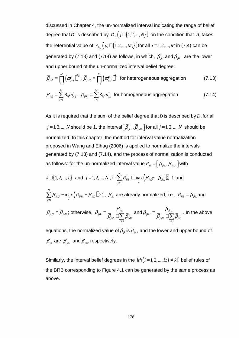
178
discussed in Chapter 4, the un-normalized interval indicating the range of belief
degree that D is described by jD ( )1,2,...,j N∈ on the condition that iA takes
the referential value of ( )1,2,...,iip i iA p M∈ for all 1,2,...,i M= in (7.4) can be
generated by (7.13) and (7.14) as follows, in which, jkLβ and jkUβ are the lower
and upper bound of the un-normalized interval belief degree:
( )1
ki
i
ML
jkL p ji
δβ ω
=
= ∏ , ( )1
ki
i
MU
jkU p ji
δβ ω
=
= ∏ for heterogeneous aggregation (7.13)
1i
ML
jkL ki p ji
β δ ω=
=∑ , 1
i
MU
jkU ki p ji
β δ ω=
=∑ for homogeneous aggregation (7.14)
As it is required that the sum of the belief degree that D is described by jD for all
1,2,...,j N= should be 1, the interval ,jkL jkUβ β for all 1,2,...,j N= should be
normalized. In this chapter, the method for interval value normalization
proposed in Wang and Elhag (2006) is applied to normalize the intervals
generated by (7.13) and (7.14), and the process of normalization is conducted
as follows: for the un-normalized interval value ,jk jkL jkUβ β β = with
1,2,...,k L∈ and 1,2,...,j N= , if ( )1
max 1N
jkL jkU jkLj
j
β β β=
+ − ≤∑ and
( )1
max 1N
jkU jkU jkLj
j
β β β=
− − ≥∑ , jkβ are already normalized, i.e., jkL jkLβ β= and
jkU jkUβ β= ; otherwise, jkLjkL
jkL ikUi j
ββ
β β≠
=+∑
and jkUjkU
jkU ikLi j
ββ
β β≠
=+∑
. In the above
equations, the normalized value of jkβ is jkβ , and the lower and upper bound of
jkβ are jkLβ and jkUβ respectively.
Similarly, the interval belief degrees in the ( )1,2,..., ;lth l L l k= ≠ belief rules of
the BRB corresponding to Figure 4.1 can be generated by the same process as
above.
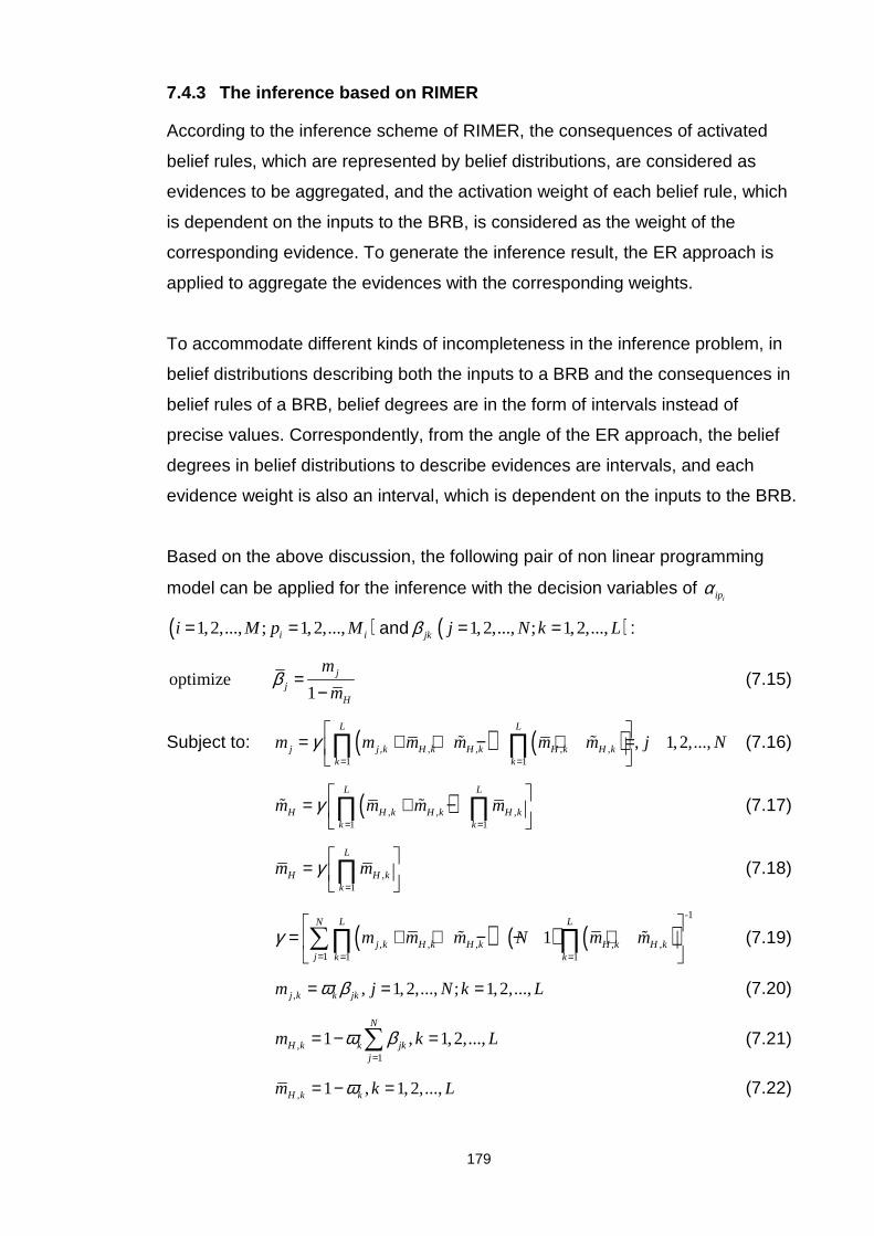
179
7.4.3 The inference based on RIMER
According to the inference scheme of RIMER, the consequences of activated
belief rules, which are represented by belief distributions, are considered as
evidences to be aggregated, and the activation weight of each belief rule, which
is dependent on the inputs to the BRB, is considered as the weight of the
corresponding evidence. To generate the inference result, the ER approach is
applied to aggregate the evidences with the corresponding weights.
To accommodate different kinds of incompleteness in the inference problem, in
belief distributions describing both the inputs to a BRB and the consequences in
belief rules of a BRB, belief degrees are in the form of intervals instead of
precise values. Correspondently, from the angle of the ER approach, the belief
degrees in belief distributions to describe evidences are intervals, and each
evidence weight is also an interval, which is dependent on the inputs to the BRB.
Based on the above discussion, the following pair of non linear programming
model can be applied for the inference with the decision variables of iipα
( )1,2,..., ; 1,2,...,i ii M p M= = and jkβ ( )1,2,..., ; 1,2,...,j N k L= = :
optimize 1
jj
H
m
mβ =
− (7.15)
Subject to: ( ) ( ), , , , ,1 1
, 1,2,...,L L
j j k H k H k H k H kk k
m m m m m m j Nγ= =
= + + − + = ∏ ∏ɶ ɶ (7.16)
( ), , ,1 1
L L
H H k H k H kk k
m m m mγ= =
= + − ∏ ∏ɶ ɶ (7.17)
,1
L
H H kk
m mγ=
= ∏ (7.18)
( ) ( ) ( )-1
, , , , ,1 1 1
1L LN
j k H k H k H k H kj k k
m m m N m mγ= = =
= + + − − + ∑∏ ∏ɶ ɶ (7.19)
, , 1, 2,..., ; 1,2,...,j k k jkm j N k Lω β= = = (7.20)
,1
1 , 1,2,...,N
H k k jkj
m k Lω β=
= − =∑ (7.21)
, 1 , 1,2,...,H k km k Lω= − = (7.22)

180
,1
1 , 1,2,...,N
H k k jkj
m k Lω β=
= − =
∑ɶ (7.23)
( )
( )1
1 1
, 1,2,...,
ki
i
ki
i
Mk
k ipi
k MLk
k ipk i
k L
δ
δ
θ αω
θ α=
= =
= =∏
∑ ∏ (7.24)
, 1,2,..., , 1,2,..., , 1,2,...,i
kip ij ii M j M k Lα α= = ∈ = (7.25)
, 1,2,..., , 1,2,...,ijL ij ijU ii M j Mα α α≤ ≤ = ∈ (7.26)
, 1,2,..., , 1, 2,...,jkL jk jkU j N k Lβ β β≤ ≤ = = (7.27)
1
1, 1,2,...,iM
ijj
i Mα=
= =∑ (7.28)
1
1, 1,2,...,N
jkj
k Lβ=
= =∑ (7.29)
In the above models, the inference scheme of RIMER is reflected by (7.15)-
(7.25), and (7.26)-(7.29) describe the constraints on decision variables.
Specifically, (7.15)-(7.23) are the equations for analytical ER approach as
introduced in Chapter 2; (7.24) is the equation to calculate activation weight of
the kth rule in the BRB according to (4.26) to (4.28); (7.25) indicates that in the
kth rule, the antecedent iA ( )1,2,...,i M= takes the referential value of ijA
( )1,2,..., ij M∈ ; (7.26) specifies the restriction on ijα , which is the belief degree
assigned to ijA ; (7.27) specifies the restriction on jkβ which can be generated by
the process Section 7.4.2; (7.28) is used to ensure that the sum of belief degree
assigned to each referential value of any antecedent iA ( )1,2,...,i M= is 1; and
(7.29) is used to ensure that the sum of all belief degrees in the kth belief rule is
1. Furthermore, if there are EIF(s), VIF(s) or BF(s) involved in the aggregation
process, ( )1,2,..., ; 1,2,...,ki k L i Mδ ∈ ∈ , kθ and ijα
( )1,2,..., , 1,2,..., ii M j M∈ ∈ in the above model should be updated/specified
according to the discussion in Chapter 6. ( )1,2,...,j j Nβ ∈ in the objective
function (7.15) is the degree of belief assigned to the grade of jD in the
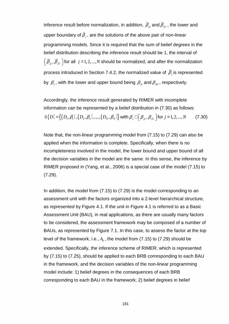
181
inference result before normalization, in addition, jLβ and jUβ , the lower and
upper boundary of jβ , are the solutions of the above pair of non-linear
programming models. Since it is required that the sum of belief degrees in the
belief distribution describing the inference result should be 1, the interval of
,jL jUβ β for all 1,2,...,j N= should be normalized, and after the normalization
process introduced in Section 7.4.2, the normalized value of jβ is represented
by jβ , with the lower and upper bound being jLβ and jHβ , respectively.
Accordingly, the inference result generated by RIMER with incomplete
information can be represented by a belief distribution in (7.30) as follows:
( ) ( ) ( ) ( ) 1 1 2 2, , , ,., , , ,N NS D D D Dβ β β= with ,j jL jUβ β β ∈ for 1,2,...,j N= (7.30)
Note that, the non-linear programming model from (7.15) to (7.29) can also be
applied when the information is complete. Specifically, when there is no
incompleteness involved in the model, the lower bound and upper bound of all
the decision variables in the model are the same. In this sense, the inference by
RIMER proposed in (Yang, et al., 2006) is a special case of the model (7.15) to
(7.29).
In addition, the model from (7.15) to (7.29) is the model corresponding to an
assessment unit with the factors organized into a 2-level hierarchical structure,
as represented by Figure 4.1. If the unit in Figure 4.1 is referred to as a Basic
Assessment Unit (BAU), in real applications, as there are usually many factors
to be considered, the assessment framework may be composed of a number of
BAUs, as represented by Figure 7.1. In this case, to assess the factor at the top
level of the framework, i.e., 0A , the model from (7.15) to (7.29) should be
extended. Specifically, the inference scheme of RIMER, which is represented
by (7.15) to (7.25), should be applied to each BRB corresponding to each BAU
in the framework, and the decision variables of the non-linear programming
model include: 1) belief degrees in the consequences of each BRB
corresponding to each BAU in the framework; 2) belief degrees in belief
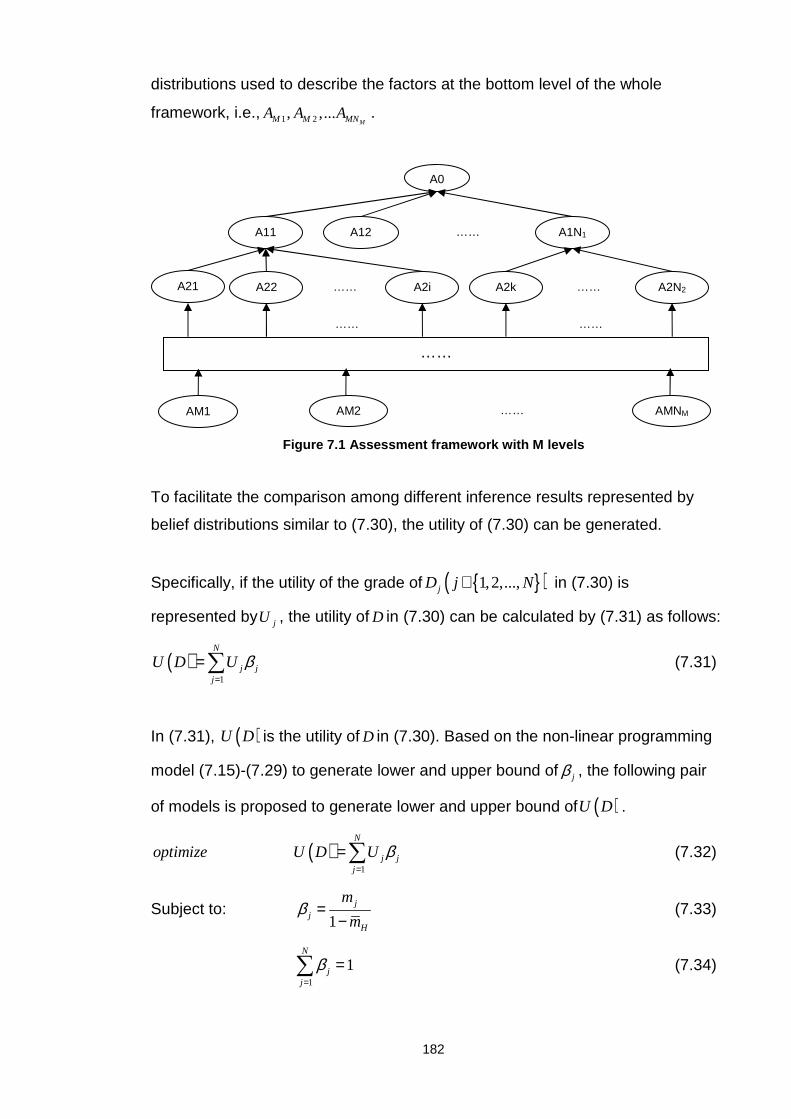
182
distributions used to describe the factors at the bottom level of the whole
framework, i.e., 1 2, ,...MM M MNA A A .
Figure 7.1 Assessment framework with M levels
To facilitate the comparison among different inference results represented by
belief distributions similar to (7.30), the utility of (7.30) can be generated.
Specifically, if the utility of the grade of ( )1,2,...,jD j N∈ in (7.30) is
represented by jU , the utility of D in (7.30) can be calculated by (7.31) as follows:
( )1
N
j jj
U D U β=
=∑ (7.31)
In (7.31), ( )U D is the utility of D in (7.30). Based on the non-linear programming
model (7.15)-(7.29) to generate lower and upper bound of jβ , the following pair
of models is proposed to generate lower and upper bound of ( )U D .
( )1
N
j jj
optimize U D U β=
=∑ (7.32)
Subject to: 1
jj
H
m
mβ =
− (7.33)
1
1N
jj
β=
=∑ (7.34)
A0
A11 A12 …… A1N1
A21 A22 …… A2i A2k …… A2N2
…… ……
……
AM1 AM2 …… AMNM

183
and (7.16)-(7.29)
In the above model, (7.16)-(7.29) and (7.33) are derived from analytical ER
approach, while the aim of (7.34) is to ensure that the sum of the belief degrees
in the belief distribution used to describe the inference result is 1.
Based on the lower and upper bound of ( )U D generated by (7.16)-(7.29) and
(7.32)-(7.34), the average of the lower and upper bound is selected as the
criterion to rank different alternatives.
Note that the model (7.16)-(7.29) and (7.32)-(7.34) can only be applied to a 2-
level hierarchical structure as represented by Figure. 4.1, to enable the model to
handle M-level hierarchical structure as represented by Figure. 7.1, the model
should be extended in a way similar to the discussion in the paragraph just
before Figure 7.1.
7.4.4 Summary
To accommodate both global and local incompleteness existing in the input
information regarding antecedents and in the knowledge on relation among
antecedents and consequences of BRBs, interval belief degrees are introduced
to describe input information and consequences of belief rules in BRBs in (7.3)
and (7.4). By extending the method for precise belief degree generation
proposed in Chapter 4, interval belief degrees in the consequence of belief rules
in BRBs are generated. Subsequently, a pair of non-linear programming models
is developed to generate inference result based on the ER approach, and for
the convenience of comparison, another pair of non-linear programming models
are developed to generate the upper and lower bound of the utilities for the
inference result and the alternative are then ranked according to the mid-point
of the corresponding utility intervals.
7.5 Case Study
In previous case studies, security assessment of a port storage area along a
CLSC against cargo theft is conducted both by the direct application of RIMER

184
in Chapter 4 and with consideration of different information aggregation patterns
under the framework of RIMER in Chapter 6. However, in both assessment
models, different kinds of incompleteness are handled in the same way,
especially, the methods applied in Chapter 4 and Chapter 6 are not capable of
handling the situation in which there is no information for one of antecedents of
a BRB, as discussed in Section 7.3.2. Therefore, in Chapter 4 and Chapter 6,
very small belief degrees are assigned to all referential values of the antecedent
without any information. For example, in a certain port in China, there is no
information regarding the Retention Period of the CCTV System, accordingly,
the belief distribution to describe the antecedent Retention Period is
approximated as (Long, 0.001), (Moderate, 0.001), (Short, 0.001). To deal with
incompleteness as above certainly brings some extent of distortion to the
security assessment results, therefore, in the case study in this chapter, the
security assessment of the 5 ports in previous chapters is conducted again,
using the methods developed in this chapter, and with the consideration of
different kinds of information aggregation patterns as discussed in Chapter 6.
Specifically, the case study begins with the illustration of the methods proposed
in this chapter based on individual BRBs, and then, the security assessment
results of the 5 ports are presented, and compared with the results generated in
previous chapters.
7.5.1 Incompleteness regarding input information of the security assessment model
As revealed by the example in Section 7.2, from an interview with a PFSO in a
certain port in China, it is known that, the access points in the port are
controlled by both electronic key-cards and traditional keys/locks, and no
access is controlled by biometric information. However, as there are many
access control points throughout the port, it is impractical to figure out how
many access control points are controlled by electronic key-cards and how
many access control points are controlled by traditional keys/locks. On the other
hand, as indicated in Appendix 3, when the access is controlled by traditional
keys/locks, the Capability of the access control system is judged as ‘Low’, when
the access is controlled by electronic key-cards, the Capability of the access
control system is considered as ‘Moderate’, and when the access is controlled
185
according to biometric information, the Capability of the access control system
is said to be ‘High’.
Therefore, according to the information collected from the PFSO, the Capability
of the access control system in the port can be represented by the following
belief distribution:
S(Capability)=(High,[0,0]), (Medium, [0,1], (Low, [0,1]) (7.35)
From (7.35), it can be seen that, the belief degree assigned to the referential
value of ‘High’ is 0, while the belief degrees assigned to both ‘Moderate’ and
‘Low’ are from 0 to 1, indicating that the capability cannot be judged as ‘High’,
and it can be judged as both ‘Medium’ and ‘Low’ to a certain degree, however,
there is no information available to specify the precise value of such belief
degrees.
According to the discussion in Section 7.2, the incompleteness presented in
(7.35) is categorized as local incompleteness. Besides local incompleteness,
global incompleteness also exists in the input information regarding the basic
factors in the security assessment model in Appendix 1. For example, as the
information on Economic Loss due to cargo theft in a certain port storage area
is not available, the belief distribution used to represent Economic Loss is:
S(Economic Loss)=(High, [0,1]), (Medium, [0,1]), (Low, [0,1] (7.36)
From (7.36), it can be inferred that, all the referential values are possible to be
used to describe Economic Loss, however, due to the lack of information, the
precise value of each belief degree cannot be determined.
From (7.35) and (7.36), it can be seen that, by introducing interval value into the
belief degrees of belief distributions to describe input information to BRBs, both
local incompleteness and global incompleteness in the input information can be
represented conveniently.

186
7.5.2 Incompleteness regarding the relation among a ntecedents and consequence in BRBs in the security assessment mode l
Apart from the incompleteness existing in the input information, the knowledge
regarding the relation among antecedents and consequence of the BRBs in the
security assessment model in Appendix 1 may also be incomplete, and as
discussed in Section 7.4.2, such incompleteness is reflected by the interval
belief degrees in the consequence of the corresponding BRBs.
For example, for Alarm System, its performance is influenced by both its
Capability and its Robustness. To model the influence using BRB, i.e., to
generate a set of belief rules to describe the influence, a set of pair-wise
comparison matrix need to be generated following the process discussed in
Section 7.4.2, and the one in Table 7.3 shows the relation between the
performance of Alarm System and its Capability when the Capability is ‘High’.
Table 7.3 Pair-wise comparison matrix for impact of Capability on Alarm System when
Capability is ‘High’
CAP=H Good Moderate Poor
Good [1, 1] [2,4]a [4,6]a
Moderate [0.25, 0.5]b [1, 1] [1,3]a
Poor [0.17, 0.25]b [0.33, 1]b [1, 1] a: Experts’ judgments b: Reciprocal of the expert’s judgments
The most obvious feature of the pair-wise comparison matrix in Table 7.3 is that,
the elements in the matrix are intervals instead of precise values. This feature is
useful in that it can provide flexibility for experts to express their judgments,
especially when they are not confident in their judgments.
Specifically, from Table 7.3, it can be found that, without considering the impact
of Robustness on Alarm System, when Capability is ‘High’, the likelihood that
the performance of the Alarm System is ‘Good’ is 2 to 4 times as the likelihood
that the Alarm System is ‘Moderate’, and 4 to 6 times as the likelihood that the
Alarm System is ‘Poor’, while the likelihood that the Alarm System is ‘Moderate’

187
is 1 to 3 times as the likelihood that the Alarm System is ‘Poor’. It is reasonable
since higher Capability can lead to better performance of an Alarm System.
To check the consistency of the interval valued pair-wise comparison matrix in
Table 7.3, Table 7.4 is generated as follows according to the discussion in
(Wang, et al., 2005):
Table 7.4 Consistency check for pair-wise compariso n matrix in Table 7.3
Judgment element i j k ik kjl l ik kju u ( )max ik kjl l ( )min ik kju u Result
12a 1 2 1 2 4
2 4 Passed 1 2 3 1.33 6
13a 1 3 1 4 6
4 6 Passed 1 3 2 2 12
23a 2 3 1 1 3
1 3 Passed 2 3 2 1 3
In Table 7.4, ija is the element in the ith row and jth column of the pair-wise
comparison matrix in Table 7.3, with its lower bound and upper bound being ijl
and iju , respectively. From Table 7.4, it can be seen that the matrix in Table 7.3
passes all the consistency tests and thus, it is a consistent interval comparison
matrix.
Further, if the priorities of grades ‘Good’, ‘Moderate’ and ‘Poor’ are represented
by Gω , Mω and Pω , respectively, according to (7.5) and (7.6), the following set of
models is built to generate the range of Gω :
Goptimize ω (7.37)
Subject to: 2 0M Gω ω− ≤ (7.38)
4 0G Mω ω− ≤ (7.39)
4 0P Gω ω− ≤ (7.40)
6 0G Pω ω− ≤ (7.41)
0P Mω ω− ≤ (7.42)
188
3 0M Pω ω− ≤ (7.43)
1G M Pω ω ω+ + = (7.44)
0, 0, 0G M Pω ω ω≥ ≥ ≥ (7.45)
By solving the model (7.37)-(7.45), we can find that [ ]0.5714,0.7059Gω ∈ .
Similarly, we can have: [ ]0.1667,0.3000Mω ∈ and [ ]0.1000,0.1667Lω ∈ . According
to the discussion in Section 7.4.3, the range of the following conditional
probabilities can be generated:
( ) [ ]0.5714,0.7059P AS G CAP H= = ∈ (7.46)
( ) [ ]0.1667,0.3000P AS M CAP H= = ∈ (7.47)
( ) [ ]0.1000,0.1667P AS P CAP H= = ∈ (7.48)
In (7.46)-(7.48), ‘AS’ stands for the performance of Alarm System, and ‘CAP’
stands for Capability.
In the same way, the probability of the performance of Alarm System on the
condition that the Robustness (ROB) is Not Robust (NR) can be generated as
follows:
( ) [ ]0.0625,0.0769P AS G ROB NR= = ∈ (7.49)
( ) [ ]0.2857,0.4000P AS M ROB NR= = ∈ (7.50)
( ) [ ]0.5333,0.6429P AS P ROB NR= = ∈ (7.51)
In addition, according to the opinion of PFSOs, for Alarm System, its Capability
and Robustness are of equal importance, which makes the weights of both
Capability and Robustness be 0.5, i.e., 0.5CAP ROBδ δ= = , therefore, according to
(4.27), 1CAP ROBδ δ= = .
Based on (7.46)-(7.51), and the fact that the performance of Alarm System is
generated by aggregating the information of its Capability and Robustness in a

189
heterogeneous way, the un-normalized probability of the performance of Alarm
System on the condition that Capability is ‘High’ and Robustness is ‘Not Robust’
can be generated by (7.52)-(7.54) as follows:
( )[ ] [ ]
,
0.5714 0.0625,0.7059 0.0769 0.0357,0.0543
P AS G CAP H ROB NR= = =
∈ × × = (7.52)
( )[ ] [ ]
,
0.1667 0.2857,0.3000 0.4000 0.0476,0.1200
P AS M CAP H ROB NR= = =
∈ × × = (7.53)
( )[ ] [ ]
,
0.1000 0.5333,0.1667 0.6429 0.0533,0.1072
P AS P CAP H ROB NR= = =
∈ × × = (7.54)
As (7.52)-(7.54) are un-normalized intervals, the normalization process
introduced in Section 7.4.3 should be conducted to the above probabilities, and
the normalized interval probabilities are:
( ) [ ], 0.1358,0.3499P AS G CAP H ROB NR= = = ∈ (7.55)
( ) [ ], 0.2276,0.5742P AS M CAP H ROB NR= = = ∈ (7.56)
( ) [ ], 0.2342,0.5627P AS P CAP H ROB NR= = = ∈ (7.57)
Therefore, the belief rule corresponding to (7.55)-(7.57) can be generated as
follows:
IF Capability is High AND Robustness is Not Robust, the performance of the
alarm system is (Good, [0.1358, 0.3499]), (Moderate, [0.2276, 0.5742]), (Poor,
[0.2342, 0.5627]).
Similarly, the other belief rules in the BRB can be generated, and the whole
BRB regarding the relation among the performance of the Alarm System, its
Capability and its Robustness can be summarized in the Table 7.5 on the next
page.
Note that, similar to the discussion in Chapter 4, some of the belief degrees in
Table 7.5 are updated according to subjective opinions of PFSOs. For example,

190
when Capability is ‘High’ and Robustness is ‘Robust’, the belief distribution
regarding performance of the Alarm System generated by the method
introduced in this chapter is (Good, [0.8573, 0.9490]), (Moderate, [0.0364,
0.1511]), (Poor, [0.0133, 0.0355]). However, according to the opinions of
PFSOs, the performance of the Alarm System should be definitely ‘High’ when
its Capability is ‘High’ and it is ‘Robust’, thus, the belief distribution is updated
as (Good, 1), (Moderate, 0), (Poor, 0). The same process is applied to the
situation when the Capability is ‘Low’ and the Robustness is ‘Not Robust’.
Table 7.5 BRB for Performance of Alarm System based on incomplete knowledge
Antecedent Consequence
Capability Robustness Performance of Alarm System
Good Moderate Poor
High Robust [1,1] [0,0] [0,0]
High Not Robust [0.1358, 0.3499] [0.2776, 0.5742] [0.2342, 0.5627]
Moderate Robust [0.3713, 0.5909] [0.3580, 0.5783] [0.0336, 0.0834]
Moderate Not Robust [0.0188, 0.0510] [0.6119, 0.8097] [0.1666, 0.3509]
Low Robust [0.3115, 0.6324] [0.1400, 0.4435] [0.1580, 0.4049]
Low Not Robust [0,0] [0,0] [1,1]
7.5.3 Inference under incomplete information
To demonstrate the inference process based on incomplete information, the
Performance of Access Control System in a certain port is assessed.
As revealed by the case study in Chapter 5, the Performance of Access Control
System is determined by its Coverage, Robustness and Capability, and the
referential values used to describe Coverage, Robustness and Capability are
listed in Table 5.1, together with the meanings of each referential value. In
addition, the current situation of the Access Control System operated in the port
is also introduced in the case study in Chapter 5. According to the current
situation, the following belief distributions can be used to describe Coverage
and Robustness:
S(Coverage)=(Wide, 0.1), (Medium, 0.1), (Limited, 0.8) (7.58)
191
S(Robustness)=(Robust, 0.8), (Not Robust, 0.2) (7.59)
As for Capability, it can be represented by the belief distribution in (7.35)
according to previous discussions.
In addition, from Appendix 6, it is known that the Performance of Access Control
System is generated by aggregating the information of its Coverage,
Robustness and Capability in a heterogeneous pattern, and there is no EIF, VIF
or BF involved in the aggregation process. Further, when the BRB regarding the
relation among Performance of Access Control System, Coverage, Robustness
and Capability is generated, there is no incompleteness involved, and the BRB
is listed in Appendix 5 as BRB 26.
According to the input information represented by (7.35), (7.58) and (7.59),
together with the BRB 26 in Appendix 5, the pair of optimization models from
(7.15) to (7.29) can be applied to generate the inference result, i.e., the
Performance of Access Control System. Note that, in this example, as the belief
degrees in the BRB are precise values, in the models from (7.15) to (7.29), the
values of ( )1,2,3; 1,2,...,18jk j kβ = = are specified in the BRB 26 in Appendix 5,
and jkβ are no longer decision variables, which makes constraints (7.27) and
(7.29) invalid.
After solving the optimization models from (7.15) to (7.29) using ‘fmincon’
function in Matlab, the following results can be generated:
0.0911GLβ = , 0.1843GHβ =
0.2528MLβ = , 0.5113MHβ =
0.3044PLβ = , 0.6561PHβ =
As discussed in Section 7.4.3, a normalization process should be conducted to
normalize the above results, and after normalization, the above results remain
unchanged, i.e., we have:
0.0911GLβ = , 0.1843GHβ =
192
0.2528MLβ = , 0.5113MHβ =
0.3044PLβ = , 0.6561PHβ =
Therefore, when the Coverage, Robustness and Capability are represented by
(7.58), (7.59), and (7.35), the performance of the Access Control System is
assessed as:
(Good, [0.0911, 0.1843]), (Moderate, [0.2528, 0.5113]),
(Poor, [0.3044, 0.6561] (7.60)
From (7.60), it can be seen that the performance is not good in general, as the
extent it can be judged as ‘Poor’ is slightly more than the extent it can be judged
as ‘Moderate’ while the extent it can be judged as ‘Good’ is very small. When
more information regarding its capability becomes available, the result in (7.60)
can be updated, and the width of the interval representing the belief degrees will
reduce accordingly.
Similar to the way to assess the performance of the Access Control System, the
overall Security Level of the port storage area against cargo theft can be
generated based on the security assessment model in Appendix 1 by extending
the model from (7.15) to (7.29), as discussed in Section 7.4.4, and the overall
security can be represented by (7.61) as follows:
(Very Low, [0.0326, 0.0836]), (Low, [0.0317, 0.0851]), (Moderate, [0.0852,
0.1968]), (High, [0.0361, 0.0864]), (Very High, [0.6064, 0.7906]) (7.61)
From (7.61), it can be inferred that, against cargo theft, the security of the port
storage area under assessment is ‘Very High’ to a large extent, however, there
is also some factors which may lead to ‘Very Low’ security level. Thus, more
analysis should be conducted to reveal such factors, and extra care should be
taken on how to improve the performance of such factors in an efficient way.
193
Further, if the utilities of ‘Very Low’, ‘Low’, ‘Moderate’, ‘High’ and ‘Very High’ are
0, 0.25, 0.5, 0.75 and 1 respectively, the utility of the port storage area
regarding its security level against cargo theft can be generated based on the
model described by (7.32)-(7.34) and (7.16)-(7.29) as follows:
( ) [ ] 0.7679, 0.8779U Security Level ∈ (7.62)
Note that (7.62) also indicates that the overall security of the port against cargo
theft is good in general, as the representative utility of Security Level, which is
the mid-point of the interval in (7.62), is 0.823.
7.5.4 Summary of security assessment result of all 5 ports
Apart from the port discussed above, security assessment is also conducted
based on the data collected from other 4 ports in both China and the UK by
considering different kinds of incomplete information, and the assessment
results are summarized in Table 7.6 in the next page, together with the security
assessment results generated in Chapter 4 by direct application of RIMER and
Chapter 6 with the consideration of different information aggregation patterns.
In Table 7.6, for each port, 3 groups of assessment results are given.
Specifically, the results in the group labelled as “D” are generated by direct
application of RIMER, as discussed in Chapter 4; the results in the group
labelled as “A” are generated with the consideration of different information
aggregation patterns, as discussed in Chapter 6; while the results in the group
labelled as “AI” are generated with the consideration of both different
information aggregation patterns and different kinds of incompleteness existing
in the information for security assessment, as discussed in this chapter.
From Table 7.6, it can be seen that, the information regarding Port 4 and Port 5
is complete, while the information regarding Port 1, Port 2 and Port 3 is
incomplete, and the extent of incompleteness can be represented by the width
of the utility interval. For the convenience of comparison, Table 7.7 in the next
page summarises the interval width for each port under each method.
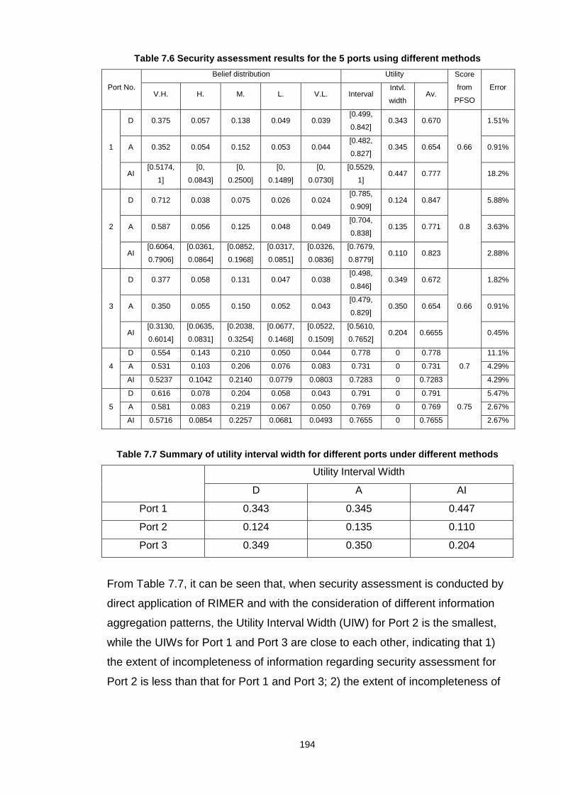
194
Table 7.6 Security assessment results for the 5 por ts using different methods
Port No.
Belief distribution Utility Score
from
PFSO
Error V.H. H. M. L. V.L. Interval
Intvl.
width Av.
1
D 0.375 0.057 0.138 0.049 0.039 [0.499,
0.842] 0.343 0.670
0.66
1.51%
A 0.352 0.054 0.152 0.053 0.044 [0.482,
0.827] 0.345 0.654 0.91%
AI [0.5174,
1]
[0,
0.0843]
[0,
0.2500]
[0,
0.1489]
[0,
0.0730]
[0.5529,
1] 0.447 0.777 18.2%
2
D 0.712 0.038 0.075 0.026 0.024 [0.785,
0.909] 0.124 0.847
0.8
5.88%
A 0.587 0.056 0.125 0.048 0.049 [0.704,
0.838] 0.135 0.771 3.63%
AI [0.6064,
0.7906]
[0.0361,
0.0864]
[0.0852,
0.1968]
[0.0317,
0.0851]
[0.0326,
0.0836]
[0.7679,
0.8779] 0.110 0.823 2.88%
3
D 0.377 0.058 0.131 0.047 0.038 [0.498,
0.846] 0.349 0.672
0.66
1.82%
A 0.350 0.055 0.150 0.052 0.043 [0.479,
0.829] 0.350 0.654 0.91%
AI [0.3130,
0.6014]
[0.0635,
0.0831]
[0.2038,
0.3254]
[0.0677,
0.1468]
[0.0522,
0.1509]
[0.5610,
0.7652] 0.204 0.6655 0.45%
4
D 0.554 0.143 0.210 0.050 0.044 0.778 0 0.778
0.7
11.1%
A 0.531 0.103 0.206 0.076 0.083 0.731 0 0.731 4.29%
AI 0.5237 0.1042 0.2140 0.0779 0.0803 0.7283 0 0.7283 4.29%
5
D 0.616 0.078 0.204 0.058 0.043 0.791 0 0.791
0.75
5.47%
A 0.581 0.083 0.219 0.067 0.050 0.769 0 0.769 2.67%
AI 0.5716 0.0854 0.2257 0.0681 0.0493 0.7655 0 0.7655 2.67%
Table 7.7 Summary of utility interval width for dif ferent ports under different methods
Utility Interval Width
D A AI
Port 1 0.343 0.345 0.447
Port 2 0.124 0.135 0.110
Port 3 0.349 0.350 0.204
From Table 7.7, it can be seen that, when security assessment is conducted by
direct application of RIMER and with the consideration of different information
aggregation patterns, the Utility Interval Width (UIW) for Port 2 is the smallest,
while the UIWs for Port 1 and Port 3 are close to each other, indicating that 1)
the extent of incompleteness of information regarding security assessment for
Port 2 is less than that for Port 1 and Port 3; 2) the extent of incompleteness of

195
information regarding security assessment for Port 1 and Port 3 are nearly the
same.
However, when security assessment is conducted by considering both different
information aggregation patterns and different kinds of incompleteness involved,
the ports can be ranked according to the value of their UIW from big to small as
follows: Port 1, Port 3 and Port 2, and there is a clear difference between UIW
of Port 3 and UIW of Port 1. In other words, according to the results in group AI,
there are clear differences among the extent of incompleteness involved in the
security assessment of Port 1, Port 2 and Port 3, and the ports can be ranked in
terms of the extent of incompleteness from large to small as: Port 1, Port 3 and
Port 2.
On the other hand, the BRBs used for security assessment for each port are the
same, and in the security assessment model in Appendix 1, there are 57 factors
in total whose information is required to be collected to conduct the security
assessment. According to the data collected, for Port 1, the information for 21
factors is missing; for Port 2, the information for 3 factors is missing; while for
Port 3, the information for 7 factors is missing. Therefore, from the real data
collected, it can be concluded that Port 1, Port 2 and Port 3 can be ranked by
the extent of incompleteness existing in the information for security assessment
from large to small as: Port 1, Port 3 and Port 2, which is consistent with the
results in group AI in Table 7.7, and different from the results in group D and
group A.
From the above discussion, it can be seen that the method proposed in this
chapter can rectify the distortion caused by inappropriate way to handle
incompleteness existing in the security assessment model in Chapter 4 and
Chapter 6, and can make the security assessment result more rational.
In addition, from the average utility of security level generated by different
methods in Table 7.6, it can be seen that for Port 2 and Port 3, the difference
between the assessment results generated by security assessment model and
the scores given by corresponding PFSOs are reduced by the introduction of

196
the method proposed in this chapter, and for Port 4 and Port 5, as there is no
incompleteness involved in the information for security assessment model, the
results generated by the method in this chapter and the results generated by
the method in Chapter 6 are the same. As for Port 1, there is a big difference
between the result generated by the method in this chapter and the score given
by the PFSO, one of the possible reasons is that, there is no information
regarding Potential Consequence due to the sensitivity of the information for
Port 1, and thus, the Potential Consequence can take the referential value of
‘None’ with the belief degree of 1 on one end and take the referential value of
‘Catastrophic’ with the belief degree of 1 on the other end. When the
consequence is described as ‘None’, the security level is ‘Very High’ with the
belief degree of 1 and thus the corresponding utility is 1. However, in reality, it is
very unlikely that there is no consequence after a theft, especially Financial
Loss. If the Financial Loss is assumed to be ‘Low’ with the belief degree of 1,
the upper bound of the utility of Security Level will be 0.7796 instead of 1, and
consequently, the corresponding average utility of Port 1 is 0.666, which is
much closer to the PFSO’s opinion, i.e., 0.66.
7.6 Conclusion
In many decision problems, it is natural that not all information needed for
decision is available due to various reasons. Therefore, the capability to handle
incompleteness in a rational way is essential to solve practical decision
problems. Correspondently, the main contribution of this chapter is to propose a
set of new methods to handle different kinds of incompleteness existing in the
CLSC security assessment model in Appendix 1.
Specifically, the contributions of this chapter can be summarized as follows: 1)
the incompleteness existing in the security assessment model is divided into 2
categories, i.e., incompleteness in input to the security assessment model and
incompleteness in the knowledge contained in the security assessment model;
2) to conveniently represent both global incompleteness and local
incompleteness existing in both the input and the knowledge, interval values are
introduced into belief degrees; 3) for incompleteness in knowledge, a new
197
process is proposed to generate belief rules with interval valued belief degrees
in the consequence, the process can provide flexibility for experts to express
their judgments; 4) a pair of non-linear programming model is proposed to
generate the inference result based on different kinds of incompleteness, and
such models can handle problems with complete or incomplete information; 5) a
pair of non-linear programming models is proposed to generate the range of
utility for inference result, i.e., security level of a port against cargo theft in this
chapter, based on the inference scheme in 4).
To validate the methods proposed in the chapter, a case study is conducted in
detail regarding security assessment of a certain port against cargo theft based
on different kinds of incomplete information. In addition, security assessment of
the other 4 ports against cargo theft is also conducted and the result of security
assessment of the 5 ports shows that the methods proposed in the chapter is
effective in solving security assessment problems with different kinds of
incomplete information, and by using the methods proposed in this chapter, the
distortion caused by inappropriate ways to handle incompleteness in previous
chapters can be rectified, which makes the results generated by the methods in
this chapter more reasonable than the results generated in previous chapters.
In addition to security assessment of port storage area against cargo theft under
the context of CLSC, the methods proposed in this chapter can be applied for
security assessment of a whole CLSC. More generally, the methods can also
be applied in many other complex assessment problems in which information
needs to be represented in various forms and there are different kinds of
incompleteness.

198
8 Chapter 8 Conclusion
Abstract
This chapter summarizes the research conducted in the thesis, its contributions
to CLSC security analysis and the implications to more general decision
problems. The limitations of the research are also discussed and the potential
future directions of the research are outlined.
8.1 Summary of the thesis
CLSC is a dominant way to transport cargo around the globe but vulnerable to
various threats during its operation. As such, the CLSC security analysis is
essential to ensure the smooth operation of CLSC. However, research on CLSC
security is relatively new and focuses on either developing policies, regulations,
and initiatives to improve CLSC security or discussing different specific security
issues of CSLC in a descriptive and subjective way. In addition, as the CLSC
security analysis has special requirements according to its characteristics,
current methods for risk/security analysis cannot be applied directly to analyze
CLSC security. In this thesis, a set of models is proposed for security analysis in
CLSC, and the models intend to answer the following two questions: how to
assess CLSC security in an analytical and rational way, and according to the
security assessment results, how to optimally develop countermeasures to
improve security level by using limited resources efficiently and effectively. By
answering the two questions, this thesis was devoted to: 1) providing a practical
tool to assist organizations and practitioners in assessing CLSC security and
developing optimal responsive measures to improve CLSC security and 2)
improving the capability of existing methods in handling complex security
analysis problems and more general decision problems under uncertainty.
Specifically, after the literature review, the research started with the
identification of factors which can influence CLSC security according to relevant
policies, regulations, codes, initiatives, etc. To facilitate the development of
analytical models for CLSC security assessment, the factors identified are
organized in a structured way through a general hierarchical model based on a
199
container’s typical voyage along a CLSC. To demonstrate the applicability of the
general hierarchical model for security assessment, the factors influencing
security of a port storage area along a CLSC against cargo theft are identified,
and then organized into a more specific hierarchical model based on the
general hierarchical model.
According to the characteristics of CLSC security assessment and the features
of RIMER in modelling and reasoning, RIMER was selected as the basic
method to assess CLSC security. To accommodate different forms of
information and different kinds of uncertainty, belief distributions were used to
model the factors. Further, a new method to generate belief degrees in BRBs
was proposed and applied for security assessment of a port storage area
against cargo theft, aiming at reducing bias and inconsistency existing in the
BRB generation process. On the basis of the BRBs generated, the security
levels of five port storage areas against cargo theft under the context of CLSC
were assessed using real data collected from both the UK and China. Through
the case studies, the applicability of RIMER for security assessment under the
context of CLSC was justified.
Based on the security assessment results, a set of models were developed
under the framework of RIMER to assist in generating optimal strategies for
resource allocation for security improvement under the context of CLSC, and
the models were then applied in the situation in which the performance of an
access control system needs to be improved to protect a port from cargo theft
under the constraint of budget. In addition, the models can also be applied to
resource allocation to improve the security of whole organizations along a
CLSC instead of individual elements within an organization, and more generally,
the models can be used to allocate limited resources based on risk/security
assessment results in broader areas, such as budget allocation for counter-
terrorism activities among different states in a country.
Subsequently, after a closer investigation to the methods for security
assessment, it was revealed that the direct application of RIMER in CLSC
security assessment have some limitations. The first limitation lies in the fact
200
that it is inappropriate to aggregate different factors in the security assessment
model in a single fixed way, as the relations among the factors have various
features. Correspondently, based on the model for security assessment of port
storage areas against cargo theft, a number of patterns for information
aggregation were identified and analyzed according to the characteristics of
relations among the factors in the model, and a set of new methods were also
developed to deal with different information aggregation patterns under the
framework of RIMER. A set of case studies about security assessment for port
storage areas against cargo theft was then conducted based on the same data
used in previous case studies to validate the aggregation patterns identified and
the methods to handle the aggregation patterns. From the results of the case
studies, it can be concluded that the consideration of different information
aggregation patterns can improve the performance of the security assessment
model in Appendix 1. Furthermore, the concept of aggregating different factors
in different patterns can be applied for security assessment of the whole CLSC
to reflect the interactions among the organizations along a CLSC.
Another limitation of the direct application of RIMER for security assessment is
the capability of RIMER in dealing with different kinds of incomplete information.
Although RIMER can handle incompleteness existing in security assessment
model, it actually transfers the incompleteness in input to BRBs into the
incompleteness in knowledge contained in BRBs, despite the fact that these two
kinds of incompleteness are different. Therefore, a set of optimization models
based on RIMER is proposed to accommodate the two kinds of incompleteness
and handle them under a unified framework. The developed models were then
applied for security assessment of port storage areas against cargo theft based
on the same set of data as those used in case studies in previous chapters, and
it was revealed that with the application of the optimization proposed models,
the distortion caused by inappropriate handling of incomplete information in
previous case studies can be rectified and the performance of the security
assessment model can be improved. More generally, the proposed optimization
models can also be applied to handle incompleteness in the security
assessment of a whole CLSC, and in other complex assessment problems with
different kinds of incompleteness.
201
In summary, the research conducted in the thesis was focused firstly on
assessing the CLSC security level in an analytical way based on a hierarchical
model developed, and then on developing optimal strategies for security
improvement under budget constraints. Due to the limitations of the security
assessment model, a set of methods were proposed to improve the capability of
the security assessment method in accommodating and handling different
information aggregation patterns and different kinds of incompleteness to make
the assessment result more rational.
In addition, the methods and models applied and proposed in this thesis can
fully meet the requirements for research of CLSC security analysis proposed in
Section 2.7, as analyzed as follows:
• RIMER is an analytical framework with strong mathematical basis. By
applying RIMER and the new models proposed in this thesis based on
RIMER, rational CLSC security assessment result can be generated,
optimal countermeasures can be developed to improve CLSC security
based on the assessment result under the constraints of limited
resources
• By introducing different information aggregation patterns and considering
economic loss in security assessment, the relations among different
organizations in a CLSC can be reflected when security of the CLSC is
assessed
• By the development of a hierarchical model for CLSC security
assessment, the factors influencing CLSC security can be identified and
organized into a structured model. By the application of belief
distributions and BRBs and the new models proposed in this thesis to
handle different kinds of incompleteness, different forms of information
with different kinds of uncertainty involved in CLCS security analysis can
be accommodated and handled
• The parameters in BRBs for CLSC security assessment are generated
according to experts’ judgments, and by applying the new method
proposed in this thesis regarding the generation of belief degrees in
202
BRBs, the bias and inconsistency involved in experts’ judgments can be
significantly reduced
• By applying the security based resource model developed in this thesis,
the resources for CLSC security improvement can be allocated optimally
based on security assessment result and the relations among the
elements involved in the resource allocation problem can be flexibly
modelled
• A number of information aggregation patterns are identified for security
assessment in CLSC according to the natures of the relations among the
factors in the CLSC security assessment model, and a set of methods
are proposed to handle the information aggregation patterns identified
8.2 Contribution of the research in the thesis
Based on the research summarized above, the contributions of the research
can be outlined as follows, from both practical and methodological points of
view.
From a practical point of view, the contributions of the research in the thesis
include:
• The factors relevant to the security of a general CLSC and the security of
a specific port storage area against cargo theft are identified and
organized into a structured way, which reveals aspects to be considered
when best practices to maintain CLSC security are developed by people
in relevant organizations and industries;
• Assistance for CLSC security assessment is provided. Although many
guidelines and principles for CLSC security assessment are proposed in
different codes, initiatives, standards, etc., the specific and practical
instructions on how to assess the security are absent. In this thesis, a
model for CLSC security assessment in general and a model for the
security assessment of a port storage area against cargo theft in
particular are proposed to organize the identified factors and facilitate
analytical CLSC security assessment. The models together with security
203
assessment methods proposed in the thesis can be used as assistance
to people in relevant organizations and industries to generate security
assessment results based on information provided;
• A method for resource allocation to improve security within a CLSC
based on security assessment results is developed. For people in
relevant organizations and industries, it is not enough to only get the
security assessment results, it is equally important to develop
countermeasures to respond to the areas with low security level with
limited resources, i.e., to improve the security level under the constraints
of limited resources. Correspondently, the method proposed in the thesis
can provide such a function, i.e., it can generate a set of practical
suggestions for security improvement to make full use of limited
resources based on security assessment results and other relevant
information provided by industrial practitioners.
Note that results generated using the models proposed in the thesis can only be
considered as a reference to their decision making on security issues in CLSC,
the adjustments on the basis of the results provided by the models in the thesis
are necessary according to specific situations of different organizations involved
in CLSCs.
From a methodological point of view, the contributions of the research in the
thesis include:
• A new process to generate belief degrees in BRBs is proposed. Although
RIMER has its unique features in modelling and reasoning under
complex environment with the simultaneous presence of various forms of
information and different kinds of uncertainty, how to generate initial
values of the parameters, especially initial belief degrees in BRBs
remains as an open and domain specific question. The process
proposed in the thesis can be considered as a tool to assist BRB
generation. By following the process, bias and inconsistency involved in
the process to generate belief degrees can be reduced significantly,
especially when the number of antecedents of BRBs or the number of

204
referential values used to describe antecedents is not trivial. Note that
bias and inconsistency can also be reduced by training parameters for
RIMER (Yang, et al., 2007) if there are data available. However, in some
situations, e.g., CLSC security analysis, available data is often
insufficient for parameter training, and the process proposed in this
thesis is especially useful;
• A new method for optimal resource allocation based on security
assessment results is proposed. For optimal resource allocation, most
strategies developed in current research are not based on the results of
risk or security assessment, and thus the resources may not be allocated
in an efficient way. In addition, most methods for optimal resource
allocation are developed on the assumption that all elements involved in
the problem can be described by precise values and relations among the
elements can always be modelled by pure mathematical functions.
Facing this situation, a new method is proposed in the thesis to optimally
allocate limited resources for security improvement based on security
assessment result. In addition, under the framework of RIMER, the
method can also accommodate different forms of information with
various kinds of uncertainty involved in the resource allocation problem
and the method can model the relations among the elements in the
problem in a flexible way. Furthermore, the method proposed can not
only be applied under the context of CLSC security analysis, but can also
be applied in many other areas in which limited resources need to be
allocated based on risk or security assessment result;
• A new concept to aggregate various factors in different patterns is
proposed and a number of new methods are developed to handle the
identified information aggregation patterns. Currently, in most MCDA
problems, information of different criteria is aggregated following a single
fixed pattern, regardless of the fact that the criteria may have different
relations. In this thesis, the relations among the factors of the security
assessment model for a port storage area against cargo theft are
analyzed in detail, based on which a number of information aggregation
patterns are identified and a set of methods is proposed under the
framework of RIMER to handle different patterns for information
205
aggregation. The concept can not only be applied for the security
assessment of a port storage area, but can also be applied to the
security assessment of the whole CLSC. Especially, when it is applied for
the security assessment of a whole CLSC, the interactions among
different organizations involved in a CLSC can be reflected conveniently.
More generally, in other MCDA problems in which relations among
criteria are complex, the concept is still valid and practical;
• A new method to handle different kinds of incompleteness is proposed.
Incomplete information is prevalent in many real decision problems, and
RIMER is a method which can accommodate and handle incompleteness.
However, RIMER can only accommodate global incompleteness and it
transfers incompleteness in inputs to BRBs into incompleteness in the
knowledge contained in BRBs. In the thesis, a way to accommodate both
local and global incompleteness and a method to handle incompleteness
in both inputs to BRBs and knowledge contained in BRBs are proposed
and applied for the security assessment of port storage areas against
cargo theft. The method can also be applied for security assessment of a
whole CLSC, and more generally, for other decision problems where
different kinds of incompleteness are prevalent and co-exist with each
other.
Note that in this thesis, the optimization models regarding security based
resource allocation in Chapter 5 and incomplete information handling in Chapter
7 are solved by the direct application of ‘fmincon’ function in Matlab, because
the scale of the problem is not large (less than 50 variables and 30 constraints).
If the optimization models proposed in this thesis are applied in other problems,
the scale of which is much larger than the scale of the problems in this thesis,
specific and more efficient algorithm need to be developed to solve the
problems.
8.3 Limitations of the research in the thesis
Although the research conducted in the thesis attempts to provide a
comprehensive and practical analysis related to security issues in CLSC and

206
thus help maintain the security of CLSC operation, due to the constraints of time
and capability, there are still several issues which are not covered by the
research and need further investigation in the future. Correspondently, the
limitations of the research can be summarized as follows:
• In the thesis, the general framework for the security assessment of a
whole CLSC is proposed, and the applicability of the framework is shown
by the case studies for the security assessment of port storage areas
along CLSCs against cargo theft. However, security assessment for
other threats faced by ports and other organizations involved in CLSCs
are not discussed in detail
• Although the interactions among different organizations involved in a
CLSC can be reflected by different information aggregation patterns as
discussed in Chapter 6 and the introduction of the factor of “Economic
Loss” as discussed in Chapter 3, there is no specific discussion on how
to model such interactions within a specific CLSC. Only after such
interactions are identified, analyzed and modelled appropriately , the
general framework for security assessment of the whole CLSC can be
fully validated
• The optimal resource allocation methods proposed in the thesis are
based on RIMER (Yang, et al., 2006). However, there are several
limitations of the direct application of RIMER in security assessment of
port storage areas against cargo theft, as discussed in Chapter 6 and
Chapter 7, and the improvement of the capability of RIMER to overcome
the limitations are not considered in the optimal resource allocation
model
• To validate the optimal resource allocation model for security
improvement based on security assessment results, the example about
improvement of access control system performance is discussed in detail.
For an access control system, the relation between budget invested and
the performance of the system can be roughly estimated by a set of pure
mathematical functions. However, if the optimal resource allocation
model is applied in a more macro level, e.g., if the security level of a
whole port involved in a CLSC need to be improved, it is difficult, if not
207
impossible, to build pure mathematical relation between resources
consumed and performance improved
• When information aggregation patterns are discussed in Chapter 6, the
discussion is based on the security assessment model for cargo theft in a
port storage area. Besides the patterns identified in Chapter 6, there may
be other patterns in security assessment for other threats faced by a port
or other organizations involved in CLSC operation. The security
assessment of the whole CLSC will be more rational after all information
aggregation patterns involved in the corresponding security assessment
models are identified and handled
• Although much effort has been put for data collection, due to the
sensitivity of the topic, only 5 sets of valid data are collected from the
ports in the UK and China regarding their security level against cargo
theft after 15 questionnaires have been sent to PFSOs around the world.
8.4 Directions of future research
Corresponding to the limitations of the research revealed above, the possible
directions of the research in the future can be outlined as follows:
• The scope of the research can be expanded. Specifically, the factors
influencing port security against other threats besides cargo theft should
be identified and organized into analytical models according to the
analysis of relations among the identified factors. Based on the analytical
models, the security level of a whole port can be assessed using the
methods proposed in the thesis. In a similar way, the security level of
other organizations involved in the CSLC should also be assessed
• Based on security assessment result regarding each organization
involved in a CLSC, the specific way to identify, analyze and model the
interactions among the organizations need to be discussed in detail to
make the assessment of the security level of a whole CLSC more
rational
• The improvements to the original RIMER method regarding its capability
to accommodate and handle different information aggregation patterns
208
and different kinds of incompleteness should be incorporated into the
optimal resource allocation model proposed in Chapter 5 to make the
resource allocation more rational
• Proper methods to flexibly model and estimate the effectiveness of
different countermeasures and the resources consumed by different
countermeasures should be investigated and developed to assist optimal
resource allocation to improve CLSC security based on security
assessment results
• A clear identification and comprehensive analysis of different information
aggregation patterns is needed under broader context, and a set of
methods to accommodate and handle the information aggregation
patterns identified should be developed
• More case studies should be conducted to validate the research in the
thesis in a broader scope, including case studies regarding other threats
faced by ports, other ports, other organizations involved in CLSCs, and a
whole CLSC.
209
References
9/11 Commission, “The 9/11 Commission Report”, 2004
J.O. Aagedal, F. Braber, T. Dimitrakos, B.A. Gran, D. Raptis and K. Stolen,
"Model-based risk assessment to improve enterprise security," Proceedings of
the Sixth International Enterprise Distributed Object Computing Conference,
Lausanne, Switzerland, pp.51-62, 2002
V. Agarwal and S. Seshadri, “Risk intermediation in supply chains”, IIE
Transactions, Vol. 32, No. 9, pp. 819-831, 2000
N.W. Arnell, E.L. Tompkins and W.N. Adger, “Eliciting Information from Experts
on the Likelihood of Rapid Climate Change”, Risk Analysis, Vol. 25, No. 6, pp.
1419–1431, 2005
ASIS, “Organizational resilience: security, preparedness, and continuity
management systems – requirements with guidance for use”, US: ASIS
International, 2009
N.J. Bahr, “System safety engineering and risk assessment”, Taylor & Francis:
London, 1997
N.O. Bakir, “A brief analysis of threats and vulnerabilities in the maritime
domain”, in I. Linkov et al. (eds.), Managing Critical Infrastructure Risks,
Springer: Netherlands, pp. 17-49, 2007
R. Banomyong, “The impact of port and trade security initiatives on maritime
supply chain management”, Maritime Policy & Management, Vol.32, No.1, pp.3-
13, 2005
G. Beliakov, A. Pradera and T. Calvo, “Aggregation Functions: A Guide for
Practitioners”, Springer, Berlin, 2007

210
Ø. Berleetal, B.E. Asbjørnslett and J.B. Rice, “Formal Vulnerability Assessment
of a maritime transportation system”, Reliability Engineering and System Safety,
Vol. 96, pp. 696-705, 2011
K. Bichou, “Security and risk-based models in shipping and ports: review and
critical analysis”, OECD International Transport Forum, Discussion Paper No.
2008-20, 2008
J.P. Brans, B. Mareschal and Ph. Vincke, “PROMETHEE: A new family of
outranking methods in multicriteria analysis”, In: J.P. Brans Editors,
“Operational Research84”, pp. 408–421, Elsevier Science Publishers,
Amsterdam, 1984
A. Brunet, “Grant Funding to State and Local Governments and Systematic
Assessment of Vulnerability”, Centre for Risk and Economic Analysis of
Terrorism Events Report, 2005
S.A. Butler, “Security attribute evaluation method: a cost-benefit approach”,
Proceedings of the 24th International Conference on Software Engineering,
Florida, U.S., pp.232-240, 2002
CBP, “Container Security Initiative”, Custom Border Protection, 2002a
CBP, “Customs-Trade Partnership Against Terrorism”, Custom Border
Protection, 2002
P.L. Chang and Y.C. Chen, “A fuzzy multi-criteria decision making method for
technology transfer strategy selection in biotechnology”, Fuzzy Sets and
Systems, Vol. 63, No. 2, pp. 131-139, 1994
C.H. Cheng, “Evaluating weapon systems using ranking fuzzy numbers”, Fuzzy
Sets and Systems, Vol. 107, No. 1, pp. 25-35, 1999

211
K.S. Chin, D.W. Tang, J.B. Yang, S. Y. Wong and H.W. Wang, “Assessing new
product development project risk by Bayesian network with a systematic
probability generation methodology”, Expert Systems with Applications, Vol. 36,
No. 6, pp. 9879-9890, 2009
S. Chopra and P. Meindl, “Supply chain management: strategy, planning and
operations”, 2nd edition, Pearson Prentice Hall: New Jersey, 2004
M. Christopher and H. Lee, “Mitigating supply chain risk through improved
confidence”, International Journal of Physical Distribution & Logistics
Management, Vol. 34, No. 5, pp. 388-96, 2004
D. Closs and E. McGarrell, “Enhancing Security Throughout the supply chain”,
IBM Center for the Business of Government Special Report Series, 2004
S. Cooperman, “Tracking Cargo”, Security, Vol. 41, No.8, pp.20–22, 2004
F.G. Cozman, “Axiomatizing noisy-OR”, Proceedings of the European
conference on artificial intelligence, Valencia, pp. 979–980, 2004
B. Das, “Generating conditional probabilities for Bayesian networks: Easing the
knowledge acquisition problem”, In Journal CoRR cs.AI/0411034, 2004
M. David, “Editorial; High-tech tracking tools secure incoming cargo”, Electronic
Design, Feb. 17, 2005
M. Detyniecki, “Fundamentals on Aggregation Operators”, University of
California, Berkeley, Technical Report, 2001
DHS, “Strategy to Enhance International Supply Chain Security”, U.S.
Department of Homeland Security, 2007

212
F.J. Diez, “Parameter adjustment in Bayes networks: The generalized noisy
OR-gate”, proceedings of the ninth annual conference on uncertainty in artificial
Intelligence, San Francisco, pp. 99–105, 1993
J. Dombi, “Basic concepts for a theory of evaluation: The aggregative operator”,
European Journal of Operational Research, Vol. 10, No. 3, pp. 282-293, 1982
D. Dubois, J.L. Marichal, H. Prade, M. Roubens and R. Sabbadin, “The use of
the discrete Sugeno integral in decision-making : a survey”, International
Journal of Uncertainty, Fuzziness and Knowledge-Based Systems, Vol. 9, No. 5,
pp. 539-561, 2001
D. Dubois, H. Prade and R. Sabbadin, “Qualitative decision theory with Sugeno
integrals”, Proceedings of the 14th Conference on Uncertainty in Artificial
Intelligence, Madison, USA, pp. 121-128, 1998
R. Dulmin and V. Mininno, “Supplier selection using a multi-criteria decision aid
method”, Journal of Purchasing and Supply Management, Vol. 9, No. 4, pp.
177-187, 2003
EC, “Regulation (EC) No. 725/2004 of the European Parliament and of the
Council on Enhancing Ship and Port Facility Security”, European Commission,
2004
EC, “Commission Regulation (EC) No. 884/2005: laying down procedures for
conducting Commission inspections in the field of maritime security”, European
Commission, 2005a
EC, “Directive 2005/65/EC of the European Parliament and of the Council on
Enhancing Port Security”, European Commission, 2005b
W. Edwards, “How to use multiattribute utility measurement for social decision
making”, IEEE Transactions on Systems, Man and Cybernetics, Vol. 7, No. 5,
pp. 326–340, 1977
213
D.G. Firesmith, “Common Concepts Underlying Safety, Security, and
Survivability Engineering”, Technical Report CMU/SEI-2003-TN-033, Carnegie
Mellon Software Engineering Institute, 2003
L.W. Fung and K.S. Fu, “An axiomatic approach to rational decision making in a
fuzzy environment”, In: L.A. Zadeh, K.S. Fu, K. Tanaka and M.Simura, editors,
“Fuzzy Sets and their Applications to Cognitive and Decision Processes”,
Academic Press, 1975.
F. Fiedrich, F. Gehbauer, and U. Rickers, “Optimized resource allocation for
emergency response after earthquake disasters”, Safety Science, Vol. 35, pp.
41-57, 2000
P. Fiorucci, F. Gaetani, R. Minciardi, R. Sacil and E. Trasforini, “Dynamic
Resource Allocation For Forest Fire Risk Management”, Proceedings of the
15th International Workshop on Database and Expert Systems Applications,
Zaragosa, Spain, 2004
J.C. Fransoo and C.Y. Lee, “Ocean container transport: an underestimated and
critical link in global supply chain performance”, Production and Operations
Management, in press, 2011
GAO, “Container Security: Expansion of Key Customs Programs Will Require
Greater Attention to Critical Success Factors”, Government Accountability
Office Report, GAO-03-770, 2003
GAO, “Container Security: A Flexible Staffing Model and Minimum Equipment
Requirements Would Improve Overseas Targeting and Inspection Efforts”,
Government Accountability Office Report, GAO-05-557, 2005a
GAO, “Risk Management, Further Refinements Needed to Assess Risks and
Prioritize Protective Measures at Ports and Other Critical Infrastructure”,
Government Accountability Office Report, GAO-06-91, 2005b

214
GAO, “Supply Chain Security: Examinations of High Risk Cargo at Foreign
Seaports Have Increased, but Improved Data Collection and Performance
Measures Are Needed”, Government Accountability Office Report, GAO-08-187,
2008
M. Garish and C. Labreuche, “A decade of application of the Choquet and
Sugeno integrals in multi-criteria decision aid”, A Quarterly Journal of
Operations Research, Volume 6, Number 1, pp. 1-44, 2007
G. Giaglis, I. Minis, A. Tatarakis and V. Ziempekis, “Minimizing logistics risk
through real time vehicle routing and mobile technologies”, International Journal
of Physical Distribution & Logistics Management, Vol. 34, No. 9, pp. 749-64,
2004
L. Godo and V. Torra, “On aggregation operators for ordinal qualitative
information”, IEEE Transactions on Fuzzy Systems, Vol. 8, No. 2, pp. 143-154,
2000
M. Grabisch, “Fuzzy integral in multicriteria decision making”, Fuzzy Sets and
Systems, Vol. 69, No. 3, pp. 279-298, 1995
M. Grabisch, “The application of fuzzy integrals in multicriteria decision making”,
European journal of operational research, Vol. 89, No. 3, pp. 445-456, 1996
M.D. Greenberg, P. Chalk, H.H. Willis, I. Khilko and D.S. Ortiz, “Maritime
Terrorism: Risk and Liability”, Santa Monica, CA: RAND Centre for Terrorism
Risk Management Policy, 2006
J.S. Helmick, “Port and maritime security: A research perspective”, Journal of
Transportation Security, Vol.1, No.1, pp.15-28, 2008
215
F. Herrera, L. Martinez and P. J. Sanchez, “Managing non-homogeneous
information in group decision making”, European Journal of Operational
Research, Vol. 166, No. 1, pp. 115-132, 2005
A.G. Hessami, ”A Systems Framework for Safety and Security: The Holistic
Paradigm”. Systems Engineering, 7(2), pp. 99-112, 2004
IMO, “International Ship and Port Facility Security Code”, International Maritime
Organization, 2002a
IMO, “Guidelines for Formal Safety Assessment for Use in the IMO Rule-
making process”, IMO, 2002b
ISO, “ISO 28000:2007: Specification for security management systems for the
supply chain”, International Organization for Standardization, 2007a
ISO, “ISO 28001:2007: Security management systems for the supply chain --
Best practices for implementing supply chain security, assessments and plans -
- Requirements and guidance”, International Organization for Standardization,
2007b
ISO, “ISO 28003:2007: Security management systems for the supply chain --
Requirements for bodies providing audit and certification of supply chain
security management systems”, International Organization for Standardization,
2007c
ISO, “ISO 28004:2007: Security management systems for the supply chain --
Guidelines for the implementation of ISO 28000”, International Organization for
Standardization, 2007d
ITPWG, “The International Shippers and Freight Forwarders Security Code”,
International Trade Procedures Working Group of United Nations Centre for
Trade Facilitation and Electronic Business, 2003
216
E. Jonsson, “An integrated framework for security and dependability”, In
Proceedings of the New Security Paradigms Workshop, pages 22–25,
Charlottesville, VA, USA, September 1998.
D.W. Keith, “When is it appropriate to combine expert judgments?”, Climatic
Change, Vol. 33, No. 2, pp. 139-143, 1996
O. Khan and B. Burnes, “Risk and supply chain management: creating a
research agenda”, The International Journal of Logistics Management, Vol. 18
No. 2, pp. 197-216, 2007
O. Khan, M. Christopher and B. Burnes, “The impact of product design on
supply chain risk: a case study”, International Journal of Physical Distribution &
Logistics Management, Vol. 38 No. 5, pp. 412-32, 2008
S.J. Kim, G.F. Deng, S.K.S. Gupta, M. Murphy-Hoye, “Intelligent networked
containers for enhancing global supply chain security and enabling new
commercial value”, the 3rd International Conference on Communication System
Software and Middleware, Bangalore, Jan.6-10, 2008, pp. 662 - 669
J.H. Kim and J. Pearl, “A computational model for combined causal and
diagnostic reasoning in inference systems”, Proceedings of the eighth
international joint conference on artificial intelligence, Karlsruhe, Germany, pp.
380–385, 1983
E.P. Klement, R. Mesiar and E. Pap, “Triangular Norms”, Kluwer Academic
Publishers, Dordrecht, 2000.
P. Knight, “Supply Chain Security Guidelines”, International Business Machines
Corporation, pp. 1-22, 2002
R. Kondaveti and A. Ganz, “Decision support system for resource allocation in
disaster management”, the 31st Annual International IEEE Engineering in

217
Medicine and Biology Society Conference, Minnesota, USA, pp. 3425-3428,
2009
C.A. Kontovas and H.N. Psaraftis, “Formal Safety Assessment: A Critical
Review”, Marine Technology, Vol. 46, No. 1, pp. 45–59, 2009
N.I. Lagoni, “The Liability of Classification Societies”, Springer-Verlag: Berlin,
2007
O. Lau, “The ten commandments of security”, Computers & Security, Vol. 17,
Issue. 2, pp. 119–123, 1998
H.L. Lee and M. Wolfe, “Supply chain security without tears”, Supply Chain
Management Review, Vol.7, No.1, pp.12-20, 2003
J.F. Lemmer and D.E. Gossink, “Recursive noisy OR – A rule for estimating
complex probabilistic interactions”, IEEE Transactions on Systems, Man and
Cybernetics – Part B: Cybernetics, Vol. 34, No. 6, pp. 2252–2261, 2004
M. Levinson, “The box: How the shipping container made the world smaller and
the world economy bigger”, Princeton University Press: Princeton, 2006
K.X. Li and K. Cullinane, “An Economic Approach to Maritime Risk
Management and Safety Regulation”, Maritime Economics and Logistics, Vol.5,
No.3, pp.268-284, 2003
J. Liu, J.B. Yang, J. Wang and H.S. Sii, “Engineering system safety analysis
and synthesis using fuzzy rule-based evidential reasoning approach”, Quality
and Reliability Engineering International, Vol. 21, pp.387-411, 2005
P. Lois, J. Wang, A. Wall and T. Ruxton, “Formal safety assessment for cruise
ships”, Tourism Management, Vol. 25, pp. 93-109, 2004

218
LRQA, “Supply Chain Security Management Systems and the role of the
Assurance Provider”, Lloyd’s Register Quality Assurance, 2009
X. Luo and N.R. Jennings, “A spectrum of compromise aggregation operators
for multi-attribute decision making”, Artificial Intelligence, Vol. 171, No. 2-3, pp.
161-184, 2007
I. Manuj and J.T. Mentzer, “Global supply chain risk management”, Journal of
Business Logistics, Vol. 29, No. 1, pp. 133-56, 2008
J.L. Marichal, “Aggregation Operators for Multi Criteria Decision Aid”, PhD
thesis, Institute of Mathematics, University of Liège, Liège, Belgium, 1998
J.L. Marichal, “An Axiomatic Approach of the Discrete Choquet Integral as a
Tool to Aggregate Interacting Criteria”, IEEE Transactions on Fuzzy Systems,
Vol. 8, No. 6, pp. 800 – 807, 2000a
J.L. Marichal, “Behavioural analysis of aggregation in multicriteria decision aid”,
In: J. Fodor, B. de Baets and P. Perny, Editors, “Preferences and Decisions
under Incomplete Knowledge”, Studies in Fuzziness and Soft Computing, Vol.
51, pp. 153–178, Physica-Verlag, Germany, 2000b
J.L. Marichal, “Aggregation of interacting criteria by means of the discrete
Choquet integral”, In: T. Calvo, G. Mayor, and R. Mesiar, editors, “Aggregation
operators: new trends and applications”, Studies in Fuzziness and Soft
Computing, Vol. 97, pp. 224–244, Physica-Verlag, Germany, 2002
J.L. Marichal, “Aggregation functions for decision making”, In: D. Bouyssou, D.
Dubois, M. Pirlot, and H. Prade, Editors: “Decision-making Process: Concepts
and Methods”, pages 673–721, Wiley, London, 2009
L. Martinez, J. Liu, D. Ruan and J.B. Yang, “Dealing with heterogeneous
information in engineering evaluation processes”, Information Sciences, Vol.
177, No. 7, pp. 1533-1542, 2007

219
E. McCormack, M. Jensen, and A. Hovde, “Evaluating the Use of Electronic
Door Seals (E-Seals) on Shipping Containers”, International Journal of Applied
Logistics, 1(4), 13-29, October-December 2010
R. Minciardi, R. Sacile and E. Trasforini, “Resource Allocation in Integrated
Preoperational and Operational Management of Natural Hazards”, Risk
Analysis, Vol. 29, No. 1, pp. 62-75, 2009
S. Monti, S and G. Carenini, G, “Dealing with the expert inconsistency in
probability elicitation”, IEEE Transactions on Knowledge and Data Engineering,
Vol. 12, No. 4, pp. 499–508, 2000
S. Noda, “Container Shipping and Security Issues: the Carriers' Responsibility
in the Fight against Terrorism”, Maritime Economics & Logistics, Vol.6, No.2,
pp.157-186, 2004
OECD, “Security in Maritime Transport: Risk Factors and Economic Impact”,
Organisation for Economic Co-operation and Development Report, 2003
OECD, “Report on Container Transport Security across modes: Executive
Summary and Conclusions”, Organisation for Economic Co-operation and
Development Report, 2004
OECD, “Container Transport Security across Modes”, Organisation for
Economic Co-operation and Development Report, 2005
R.R. Pai, V.R. Kallepalli, R.J. Caudill and M.C. Zhou, “Methods toward supply
chain risk analysis”, IEEE International Conference on Systems, Man and
Cybernetics, Vol.5, Washington, U.S., pp. 4560- 4565, 2003
U. Paulsson, “Managing risks in supply chains: an article review”, Presented at
NOFOMA, Oulu, Finland, 2003
220
J. Pearl, “Probabilistic Reasoning in Intelligent Systems: Networks of Plausible
Inference”, San Mateo: Morgan Kaufmann, 1988
PECC, “Study on the Mutually Supportive Advancement of APEC’S Trade
Facilitation and Secure Trade Goals post September 11”, Analysis and Case
Studies prepared for APEC, Singapore Pacific Economic Cooperation Council,
2004
M. Perry, “Natural disaster management planning: a study of logistics managers
responding to the tsunami”, International Journal of Physical Distribution &
Logistics Management, Vol. 37, No. 5, pp. 409-33, 2007
C.H. Piersall, “Securing the global supply chain”, ISO Focus, October, pp.33-35,
2007
C.A. Pinto, G. Rabadi and W.K. Talley, “U.S. Port Security”, in W.K. Talley.
(eds.), “Maritime Safety Security and Piracy”, Informa: London, 2008
H.N. Psaraftis, “EU Ports Policy: Where do we Go from Here?”, Maritime
Economics & Logistics, Vol.7, No.1, pp. 73-82, 2005
L. Quadrifoglio, “A bottom-up risk-based resource allocation methodology to
counter terrorism”, International Journal of Society Systems Science, Vol. 1, No.
1, pp. 4-25, 2008
S. Rao and T. Goldsby, “Supply chain risks: a review and typology”, The
International Journal of Logistics Management, Vol. 20, No. 1, pp. 97-123,
2009
C.S. Reifel, “Quantitative Risk Analysis for Homeland Security Resource
Allocation”, MSc Thesis, Naval Postgraduate School, 2006
J. Ren, I. Jenkinson, H.S. Sii, J. Wang, D.L. Xu and J.B. Yang, “An offshore
safety assessment framework using fuzzy reasoning and evidential synthesis

221
approaches”, Journal of Marine Engineering & Technology, No.A6, pp.3-16,
2005.
J. Ren, J. Wang, I. Jenkinson, D. L. Xu, J. B. Yang, “An offshore risk analysis
method using fuzzy Bayesian network”, Journal of Offshore Mechanics and
Arctic Engineering, Vol.131, No.4, 2009.
W. Robert and J.D. Kelly, “Containing the Threat: Protecting the Global Supply
Chain through Enhanced Cargo Container Security”, The Reform Institute,
reform brief, 2007
T. Rosqvist and R. Tuominen, “Qualification of Formal Safety Assessment: an
exploratory study”, Safety Science, Vol. 42, pp. 99–120, 2004
B. Roy, “Classement et choix en présence de points de vue multiples: la
méthode ELECTRE”, Revue Francaise d’Informatique et de Recherche
Opérationnelle, Vol. 8, pp. 57–75, 1968
V.D. Rugy, “What does homeland security spending buy?”, working paper No.
107, American Enterprise Institute for Public Policy Research, 2005
L.T. Saaty, “The Analytic Hierarchy Process”, McGraw-Hill: New York. 1980.
R. Sarathy, “Security and the Global Supply Chain”, Transportation journal, Vol.
45, No. 4, pp. 28-51, 2006
G. Shafer, “A mathematical theory of evidence”, Princeton, N.J.: Princeton
University Press, 1976
S. Schocken, “Ratio-scale elicitation of degrees of support”, Working Paper, IS-
93-30, Stern School of Business, New York University, 1993

222
H.S. Sii, J. Wang, A.G. Eleye-Datubo, J.B. Yang and J. Liu, “Safety assessment
of FPSO turret-mooring system using approximate reasoning and evidential
reasoning”, Journal of Marine Technology, Vol.42, No.2, pp.88-102, 2005
C.G. Soares and A.P. Teixeira, “Risk assessment in maritime transportation”,
Reliability Engineering and System Safety, Vol. 74, pp. 299-309, 2001
K. Sørby, “Relationship between security and safety in a security-safety critical
system: Safety consequences of security threats”, Master thesis, Norges
Teknisk-Naturvitenskapelige Universitet, Trondheim, Norway, 2003
D. Stasinopoulos, “Maritime Security – The Need for a Global Agreement”,
Maritime Economics & Logistics, Vol. 5, No.3, pp.311-320, 2003
G. Stoneburner, A. Goguen and A. Feringa, “Risk management guide for
information technology systems”, Technical Report 800-30, National Institute of
Standards and Technology, 2002
C.Q. Tan and X.H. Chen, “Induced Choquet Ordered Averaging Operator and
Its Application to Group Decision Making”, International Journal of Intelligent
Systems, Vol. 25, pp. 59–82, 2010
C. Tang, “Robust strategies for mitigating supply chain disruptions”,
International Journal of Logistics Research and Applications, Vol.9, No.1, pp.33-
45, 2006
TAPA, “Freight Suppliers Minimum Security Requirements”, Transported Asset
Protection Association, 2011
TAPA, “Freight Suppliers Minimum Trucking Security Requirements”,
Transported Asset Protection Association, 2008
223
B. Tomlin, “On the value of mitigation and contingency strategies for managing
supply chain disruption risks”, Management Science, Vol. 52, No. 5, pp. 639-57,
2006
V. Torra, “Aggregation operators and models”, Fuzzy Sets and Systems, Vol.
156, No. 3, pp. 407–410, 2005
D.R. Towill, “The impact of business policy on bullwhip induced risk in supply
chain management”, International Journal of Physical Distribution & Logistics
Management, Vol. 35, No. 8, pp. 555-75, 2005
P. Tirschwell, "An opportunity for container seals," Journal of Commerce, Feb.
7, 2005.
TRANSEC, “A brief overview of the United Kingdom National Maritime Security
Programme”, Department of Transport, the UK, 2011
D. Tsamboulas, “Terrorism and the Threat to Multimodal Transport – An
Overview”, in M. Bell, et al. (eds.), Security and Environmental Sustainability of
Multimodal Transport, Springer: Netherlands, pp.3-22, 2010
V.M.R. Tummala and H. Ling, “A note on the computation of the mean random
consistency index of the Analytic Hierarchy Process (AHP)”, Theory and
Decision, Vol. 44, pp. 221–230, 1998
G.H. Tzeng, Y.P. Ou Yang, C.T. Lin and C.B. Chen, “Hierarchical MADM with
fuzzy integral for evaluating enterprise intranet web sites”, Information Sciences,
Vol. 169, No. 3-4, pp. 409-426, 2005
S.T. Ung, “The Development of Safety and Security Assessment Techniques
and their Application to Port Operations”, PhD Thesis, Liverpool John Moores
University, 2007

224
U.S. Congress, “Security and Accountability For Every Port Act”, Public Law,
109–347, 2006
U.S. Maritime Administration, “Report of the United States Mobile Training
Team: Regional Course on Port Security for Caribbean Countries”, Washington,
D.C.: U.S. Government Printing Office, 2002
J. Wang, “The current status and future aspects in formal ship safety
assessment”, Safety Science, Vol. 38, pp. 19-31, 2001
Y.M. Wang, T.M.S. Elhagc, “On the normalization of interval and fuzzy weights”,
Fuzzy Sets and Systems, Vol. 157, pp. 2456 – 2471, 2006
J. Wang and P. Foinikis, “Formal safety assessment of containerships”, Marine
Policy, Vol.25, No.2, pp.143-157, 2001
C. Wang and S. Webster, “Channel coordination for a supply chain with a risk
neutral manufactures and a loss averse retailer”, Decision Sciences, Vol. 38, No.
3, pp. 361-89, 2007
Y. M. Wang, J. B. Yang and D. L. Xu, “Interval weight generation approaches
based on consistency test and interval comparison matrices”, Applied
Mathematics and Computation, Vol.167, pp.252–273, 2005
Y. M. Wang, J. B. Yang and D. L. Xu, “Environmental Impact Assessment Using
the Evidential Reasoning Approach”, European Journal of Operational
Research, Vol.174, No.3, pp.1885-1913, 2006
WCO, “SAFE Framework of Standards”, World Customs Organization, 2007
H.H. Willis and D.S. Ortiz, “Evaluating The Security Of The Global
Containerized Supply Chain”, RAND Technical Report Series, TR-214-RC,
2004
225
M. Wilson, “The impact of transportation disruptions on supply chain
performance”, Transportation Research, Part E, Vol. 43, No. 4, pp. 295-320,
2007
K.J. Wydajewski and B.L. White, “Processes and techniques for providing
critical data to first responders to maritime security incidents”, Oceans 2002
IEEE/MTS Conference Proceedings, Vol.2, Mississippi, U.S., pp.1180- 1190,
2002
Z.S. Xu, “Intuitionistic Fuzzy Aggregation Operators”, IEEE Transactions on
Fuzzy Systems, Vol. 15, No. 6, pp. 1179 – 1187, 2007
Z. S. Xu and Q. L. Da, “An overview of operators for aggregating information”,
International Journal of Intelligent Systems, Vol. 18, No. 9, pp. 953–969, 2003
D. L. Xu, J. B. Yang and Y. M. Wang, “The evidential reasoning approach for
multiple attribute decision analysis using interval belief degrees”, European
Journal of Operational Research, Vol.175, No.1, pp.35-66, 2006.
Y.Y. Yager, “On ordered weighted averaging aggregation operators in multi
criteria decision making”, IEEE Transactions on Systems, Man and Cybernetics,
Vol.18, No. 1, pp. 183 – 190, 1988
Y.Y. Yager, “Induced aggregation operators”, Fuzzy Sets and Systems, Vol.
137, No. 1, pp. 59-69, 2003
J. B. Yang, “Rule and utility based evidential reasoning approach for multiple
attribute decision analysis under uncertainty”, European Journal of Operational
Research, Vol. 131, No.1, pp. 31-61, 2001.
Y.C. Yang, “Risk management of Taiwan’s maritime supply chain security”,
Safety Science, Vol. 49, pp. 382-393, 2011
226
Z.L. Yang, “Risk Assessment and Decision Making of Container Supply Chains”,
PhD Thesis, Liverpool John Moores University, 2006
J. B. Yang, J. Liu, J. Wang, H. S. Sii and H. W. Wang, “A belief rule-base
inference methodology using the evidential reasoning approach – RIMER”,
IEEE Transactions on Systems, Man, and Cybernetics – Part A, Vol.36, No.2,
pp.266- 285, 2006.
J. B. Yang, J. Liu, D. L. Xu, J. Wang and H. W. Wang, “Optimization models for
training belief rule based systems”, IEEE Transactions on Systems, Man, and
Cybernetics – Part A, Vol.37, No.4, pp.569-585, 2007
J.B. Yang and M.G. Singh, "An evidential reasoning approach for multiple
attribute decision making with uncertainty", IEEE Transactions on Systems,
Man, and Cybernetics, Vol.24, No.1, pp.1-18, 1994
J.B. Yang and D.L. Xu, “On the evidential reasoning algorithm for multi-attribute
decision analysis under uncertainty”, IEEE Transactions on Systems, Man, and
Cybernetics - Part A: Systems and Humans, Vol.32, No.3, pp.289-304, 2002
C.H. Yeh, Y.H. Chang, “Modelling subjective evaluation for fuzzy group
multicriteria decision making”, European Journal of Operational Research, Vol.
194, No. 2, pp. 464-473, 2009
W.J. Yoon, S.H. Chung, S.J. Lee and Y.S. Moon, "Design and Implementation
of an Active RFID System for Fast Tag Collection," 7th IEEE International
Conference on Computer and Information Technology, Fukushima Prefecture,
Japan, pp.961-966, 2007
Z. J. Zhou, C. H. Hu, D. L. Xu, J. B. Yang and D. H. Zhou, “New model for
system behaviour prediction based on belief-rule-based systems”, Information
Sciences, Vol.180, pp.4834–4864, 2010.
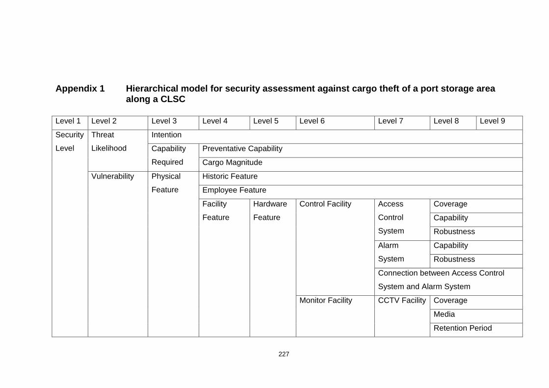
227
Appendix 1 Hierarchical model for security assessme nt against cargo theft of a port storage area along a CLSC
Level 1 Level 2 Level 3 Level 4 Level 5 Level 6 Level 7 Level 8 Level 9
Security
Level
Threat
Likelihood
Intention
Capability
Required
Preventative Capability
Cargo Magnitude
Vulnerability Physical
Feature
Historic Feature
Employee Feature
Facility
Feature
Hardware
Feature
Control Facility Access
Control
System
Coverage
Capability
Robustness
Alarm
System
Capability
Robustness
Connection between Access Control
System and Alarm System
Monitor Facility CCTV Facility Coverage
Media
Retention Period

228
Lighting
Facility
Coverage
Capability
Software Feature
Intervention
Measures
Preventative
Measures
Managerial
Measures
Regulations General
regulations
regarding
overall
security
Application of ISPS
Code
Regulations for security
culture
Regulations
regarding
access
control
Towards current
employees
Towards terminated
employees
Towards visitors
Regulations
regarding
procedure
control
Procedure for stuffing
and loading/unloading
Procedure for security
incident report
Management on
Regulations
Monitor on execution status of
regulations
Audit on execution status of regulations

229
Update on regulations
Operative
Measures
Operations relevant
to access control
Photo-ID badge
Key/Key Card
Operations relevant
to employee
training/auditing
Training of employee
Auditing of current status of employee
Operations relevant
to records
Keeping of
Records
Security
system
related
records
Logs of
alarm
system
Logs of
access
control
system
Employee
related
records
Records of
emergency
contact
Records of
employee
training
Records of

230
terminated
employees
in recent 3
years
Protection of Records
Management of Records
Operations relevant
to security related
equipments
Control of cargo-handling equipments
Test/maintenance/repair for security
systems
UPS equipments or other forms of
emergency power supply of security
systems
Operations relevant
to other issues
Cargo
Inspection
Inspection on containers
Inspection on trash
Vulnerability assessment
Guarding and patrolling
Responsive
Measures
Response
Activity
Development of contingency plan
Update of contingency plan
Drill on contingency plan
Response Rescue Facility Capability

231
Facility Availability
Communication Facility
Recovery Measures
Potential
Consequence
Human Loss
Financial Loss
Corporate Image Loss
Economic Loss
Environmental Loss
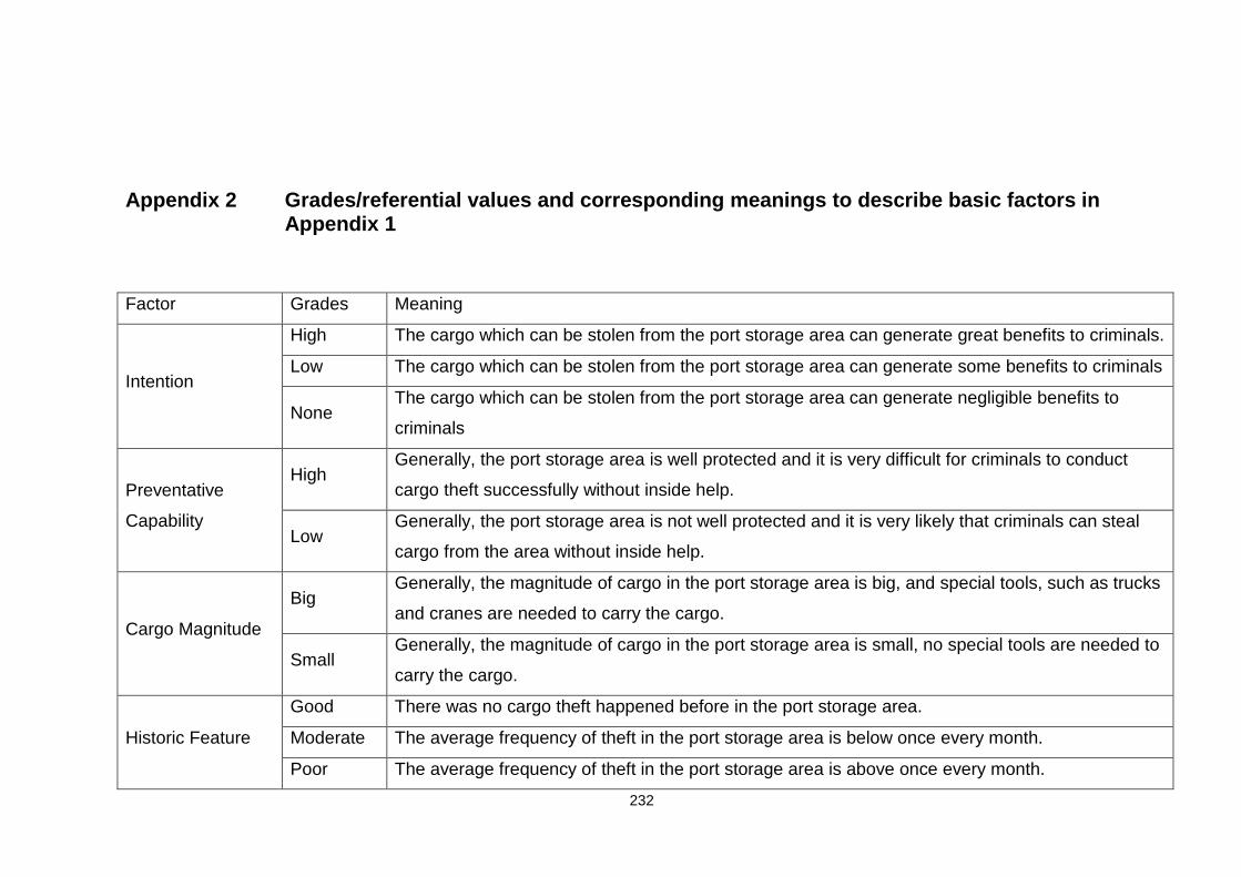
232
Appendix 2 Grades/referential values and correspond ing meanings to describe basic factors in Appendix 1
Factor Grades Meaning
Intention
High The cargo which can be stolen from the port storage area can generate great benefits to criminals.
Low The cargo which can be stolen from the port storage area can generate some benefits to criminals
None The cargo which can be stolen from the port storage area can generate negligible benefits to
criminals
Preventative
Capability
High Generally, the port storage area is well protected and it is very difficult for criminals to conduct
cargo theft successfully without inside help.
Low Generally, the port storage area is not well protected and it is very likely that criminals can steal
cargo from the area without inside help.
Cargo Magnitude
Big Generally, the magnitude of cargo in the port storage area is big, and special tools, such as trucks
and cranes are needed to carry the cargo.
Small Generally, the magnitude of cargo in the port storage area is small, no special tools are needed to
carry the cargo.
Historic Feature
Good There was no cargo theft happened before in the port storage area.
Moderate The average frequency of theft in the port storage area is below once every month.
Poor The average frequency of theft in the port storage area is above once every month.

233
Employee Feature Good There is no employee in the port storage area who was involved in cargo theft before.
Poor There are employees in the port storage area who were involved in cargo theft before
Access Control
System Coverage
Wide It covers all office entrances, all storage area entrances/exits and the areas between office and
storage area
Moderate It covers most office entrances and most storage area entrances/exits
Limited It only covers most office entrances or most storage area entrances/exits
Access Control
System Capability
High The access is controlled by biometric systems
Moderate The access is controlled by electric systems
Low The access is controlled by traditional locks/keys
Access Control
System
Robustness
Robust There is almost no failure or error occurring during the operation of the system
Not Robust Failure and error occurs from time to time during the operation of the system
Alarm System
Capability
High The alarm system is sensitive with few false alarms, and the alarm information can be sent to
relevant security staff once the alarm system is triggered.
Moderate The alarm system is sensitive with few false alarms
Low Alarm system is not sensitive, or with a number of false alarms.
Alarm System
Robustness
Robust Alarms are difficult to be disabled; a backup system will be effective immediately after it is
disabled.
Not robust Alarms are easily to be disabled.
Connection Yes Alarm system can be triggered automatically once access control system is breached

234
between access
control system and
alarm system
No Alarm system cannot be triggered automatically after access control system is breached
CCTV Coverage
Wide CCTV covers all access control points, all loading/unloading areas and all storage yards.
Moderate CCTV covers all access control points
Limited Not all access control points are covered by CCTV system.
CCTV Media VCR CCTV information is recorded by VCR
DVR CCTV information is recorded by DVR
CCTV Retention
period
Long 50 days
Medium 40 days
Short 30 days
Lighting Coverage
Wide Lighting facility illuminates all entrances/exits, all loading/unloading areas
Moderate Lighting facility illuminates all entrances/exits and most loading/unloading areas
Limited Lighting facility does not illuminate all entrances/exits
Lighting Capability
High All vehicles and individuals are clearly identifiable under the lighting area through CCTV
Moderate Vehicles and individuals are identifiable in most cases under the lighting area through CCTV
Low Vehicles and individuals can be barely identified under lighting area through CCTV
Software Feature Good In history, there was no breach into the information system operated in the storage area
Poor In history, there were some breaches into the information system operated in the storage area
Application of Yes ISPS Code is applied in the port

235
ISPS Code No ISPS Code is not applied in the port
Regulations for
security culture
Effective There is a set of regulations developed to create and maintain security culture, and most
employees can realize the importance of security for the operation in the port
Not
Effective
There is a set of regulations developed to create and maintain security culture, however,only few
employees realize the importance of security for the operation in the port
None There is no regulations developed to create or maintain security culture
Regulations
regarding access
control towards
current employees
Yes There is a set of regulations developed for access control towards current employees
No There is no regulation developed for access control towards current employees
Regulations
regarding access
control towards
terminated
employees
Yes There is a set of regulations developed for access control towards terminated employees
No There is no regulation developed for access control towards terminated employees
Regulations
regarding access
control towards
visitors
Yes There is a set of regulations developed for access control towards visitors
No There is no regulation developed for access control towards visitors
Regulations on Yes There is a set of regulations developed on procedure for stuffing and loading/unloading

236
procedure for
stuffing and
loading/unloading
No There is no regulation developed on procedure for stuffing and loading/unloading
Regulations on
procedure for
security incident
report
Yes There is a set of regulations developed on procedure for security incident report
No There is no regulation developed on procedure for security incident report
Monitor on
execution status of
regulations
Yes Yes, the execution status of regulations is monitored
No No, the execution status of regulations is not monitored
Audit on execution
status of
regulations
Yes Yes, the execution status of regulations is audited
No No, the execution status of regulations is not audited
Update on
Regulations
Yes The regulations are updated regularly and when necessary
No The regulations are not updated
Application of
Photo-ID Badge
Well
applied All employees and contractors are issued with a photo-ID badge
Applied Not all employees and contractors are issued with a photo-ID badge
Not
applied No photo-ID badge is applied.
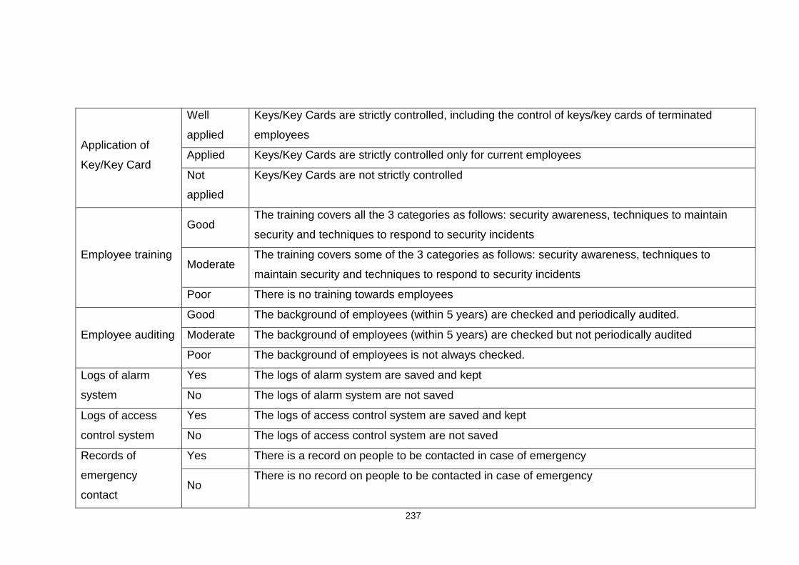
237
Application of
Key/Key Card
Well
applied
Keys/Key Cards are strictly controlled, including the control of keys/key cards of terminated
employees
Applied Keys/Key Cards are strictly controlled only for current employees
Not
applied
Keys/Key Cards are not strictly controlled
Employee training
Good The training covers all the 3 categories as follows: security awareness, techniques to maintain
security and techniques to respond to security incidents
Moderate The training covers some of the 3 categories as follows: security awareness, techniques to
maintain security and techniques to respond to security incidents
Poor There is no training towards employees
Employee auditing
Good The background of employees (within 5 years) are checked and periodically audited.
Moderate The background of employees (within 5 years) are checked but not periodically audited
Poor The background of employees is not always checked.
Logs of alarm
system
Yes The logs of alarm system are saved and kept
No The logs of alarm system are not saved
Logs of access
control system
Yes The logs of access control system are saved and kept
No The logs of access control system are not saved
Records of
emergency
contact
Yes There is a record on people to be contacted in case of emergency
No There is no record on people to be contacted in case of emergency
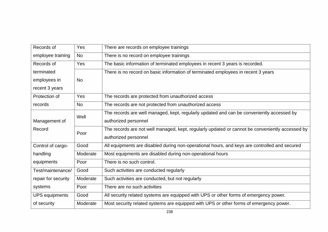
238
Records of
employee training
Yes There are records on employee trainings
No There is no record on employee trainings
Records of
terminated
employees in
recent 3 years
Yes The basic information of terminated employees in recent 3 years is recorded.
No
There is no record on basic information of terminated employees in recent 3 years
Protection of
records
Yes The records are protected from unauthorized access
No The records are not protected from unauthorized access
Management of
Record
Well The records are well managed, kept, regularly updated and can be conveniently accessed by
authorized personnel
Poor The records are not well managed, kept, regularly updated or cannot be conveniently accessed by
authorized personnel
Control of cargo-
handling
equipments
Good All equipments are disabled during non-operational hours, and keys are controlled and secured
Moderate Most equipments are disabled during non-operational hours
Poor There is no such control.
Test/maintenance/
repair for security
systems
Good Such activities are conducted regularly
Moderate Such activities are conducted, but not regularly
Poor There are no such activities
UPS equipments
of security
Good All security related systems are equipped with UPS or other forms of emergency power.
Moderate Most security related systems are equipped with UPS or other forms of emergency power.
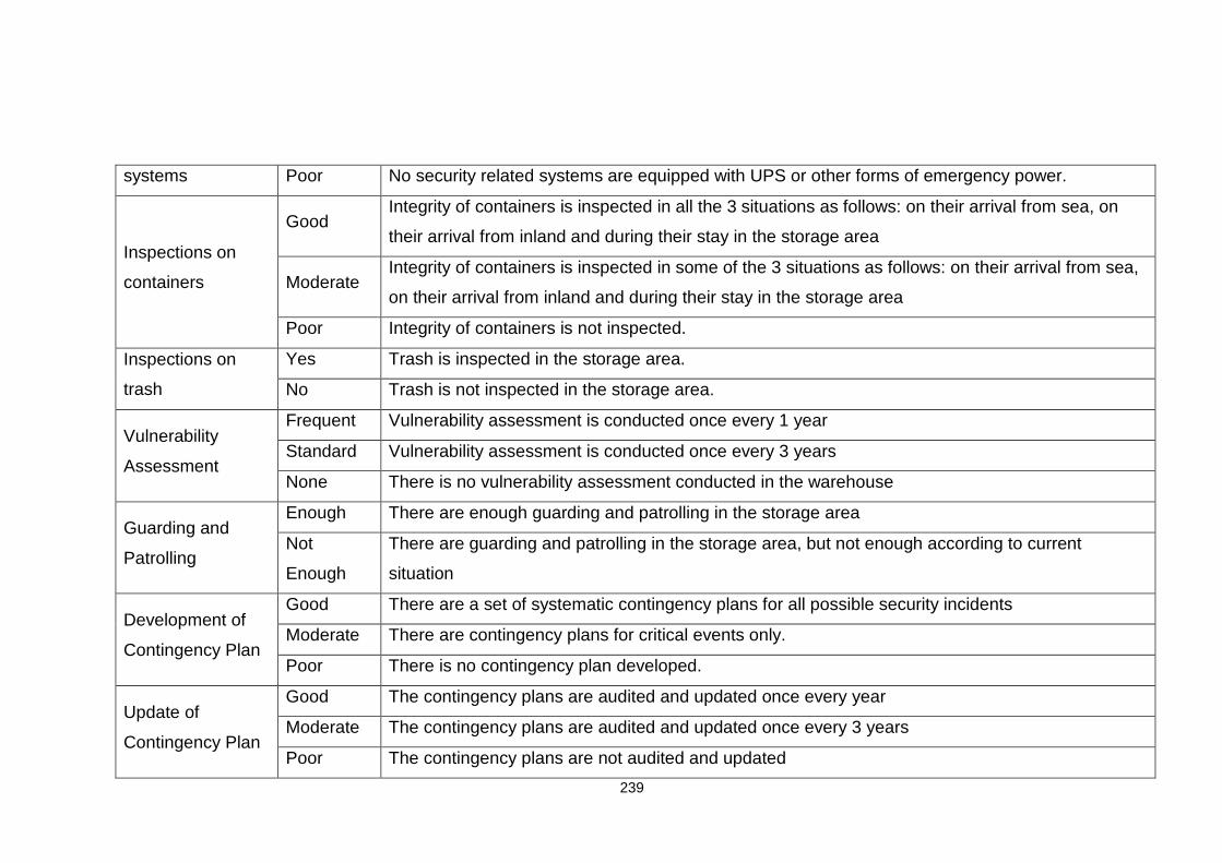
239
systems Poor No security related systems are equipped with UPS or other forms of emergency power.
Inspections on
containers
Good Integrity of containers is inspected in all the 3 situations as follows: on their arrival from sea, on
their arrival from inland and during their stay in the storage area
Moderate Integrity of containers is inspected in some of the 3 situations as follows: on their arrival from sea,
on their arrival from inland and during their stay in the storage area
Poor Integrity of containers is not inspected.
Inspections on
trash
Yes Trash is inspected in the storage area.
No Trash is not inspected in the storage area.
Vulnerability
Assessment
Frequent Vulnerability assessment is conducted once every 1 year
Standard Vulnerability assessment is conducted once every 3 years
None There is no vulnerability assessment conducted in the warehouse
Guarding and
Patrolling
Enough There are enough guarding and patrolling in the storage area
Not
Enough
There are guarding and patrolling in the storage area, but not enough according to current
situation
Development of
Contingency Plan
Good There are a set of systematic contingency plans for all possible security incidents
Moderate There are contingency plans for critical events only.
Poor There is no contingency plan developed.
Update of
Contingency Plan
Good The contingency plans are audited and updated once every year
Moderate The contingency plans are audited and updated once every 3 years
Poor The contingency plans are not audited and updated
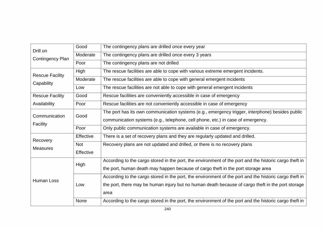
240
Drill on
Contingency Plan
Good The contingency plans are drilled once every year
Moderate The contingency plans are drilled once every 3 years
Poor The contingency plans are not drilled
Rescue Facility
Capability
High The rescue facilities are able to cope with various extreme emergent incidents.
Moderate The rescue facilities are able to cope with general emergent incidents
Low The rescue facilities are not able to cope with general emergent incidents
Rescue Facility
Availability
Good Rescue facilities are conveniently accessible in case of emergency
Poor Rescue facilities are not conveniently accessible in case of emergency
Communication
Facility
Good The port has its own communication systems (e.g., emergency trigger, interphone) besides public
communication systems (e.g., telephone, cell phone, etc.) in case of emergency.
Poor Only public communication systems are available in case of emergency.
Recovery
Measures
Effective There is a set of recovery plans and they are regularly updated and drilled.
Not
Effective
Recovery plans are not updated and drilled, or there is no recovery plans
Human Loss
High According to the cargo stored in the port, the environment of the port and the historic cargo theft in
the port, human death may happen because of cargo theft in the port storage area
Low
According to the cargo stored in the port, the environment of the port and the historic cargo theft in
the port, there may be human injury but no human death because of cargo theft in the port storage
area
None According to the cargo stored in the port, the environment of the port and the historic cargo theft in
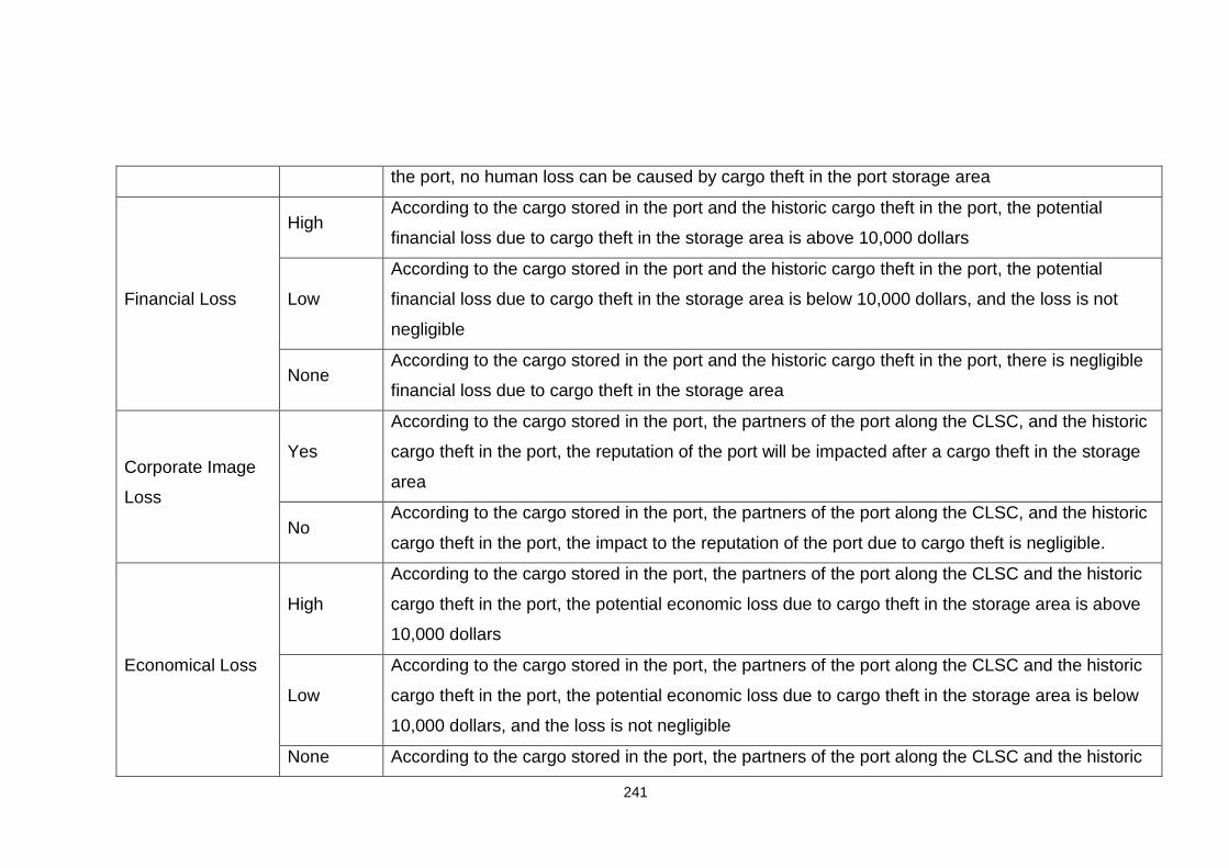
241
the port, no human loss can be caused by cargo theft in the port storage area
Financial Loss
High According to the cargo stored in the port and the historic cargo theft in the port, the potential
financial loss due to cargo theft in the storage area is above 10,000 dollars
Low
According to the cargo stored in the port and the historic cargo theft in the port, the potential
financial loss due to cargo theft in the storage area is below 10,000 dollars, and the loss is not
negligible
None According to the cargo stored in the port and the historic cargo theft in the port, there is negligible
financial loss due to cargo theft in the storage area
Corporate Image
Loss
Yes
According to the cargo stored in the port, the partners of the port along the CLSC, and the historic
cargo theft in the port, the reputation of the port will be impacted after a cargo theft in the storage
area
No According to the cargo stored in the port, the partners of the port along the CLSC, and the historic
cargo theft in the port, the impact to the reputation of the port due to cargo theft is negligible.
Economical Loss
High
According to the cargo stored in the port, the partners of the port along the CLSC and the historic
cargo theft in the port, the potential economic loss due to cargo theft in the storage area is above
10,000 dollars
Low
According to the cargo stored in the port, the partners of the port along the CLSC and the historic
cargo theft in the port, the potential economic loss due to cargo theft in the storage area is below
10,000 dollars, and the loss is not negligible
None According to the cargo stored in the port, the partners of the port along the CLSC and the historic
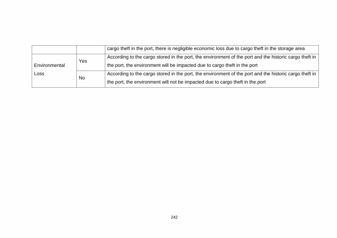
242
cargo theft in the port, there is negligible economic loss due to cargo theft in the storage area
Environmental
Loss
Yes According to the cargo stored in the port, the environment of the port and the historic cargo theft in
the port, the environment will be impacted due to cargo theft in the port
No According to the cargo stored in the port, the environment of the port and the historic cargo theft in
the port, the environment will not be impacted due to cargo theft in the port

243
Appendix 3 Grades/values for the non-basic factors in Appendix 1
Factor Grades Factor Grades Factor Grades Factor Grades Factor Grades
Security
Level
Very
High
Threat
Likelihood
Quite
likely
Vulnerability
Vulnerable
Potential
Consequence
Catastrophic
Capability
Required
High High Severe
Medium Likely Moderate Moderate
Low Not likely Not
Vulnerable
Not severe Low
Very Low Impossible None
Physical
Feature
Good
Intervention
Measures
Effective
Facility
Feature
Good
Preventative
Measures
Effective
Responsive
Measures
Effective
Moderate Moderate Moderate Moderate Moderate
Poor Not
Effective Poor
Not
Effective
Not
Effective
Hardware
Feature
Good
Managerial
Measures
Effective
Operative
Measures
Effective
Response
Activity
Effective
Response
Facility
Good
Moderate Moderate Moderate Moderate Moderate
Poor Not
Effective
Not
Effective
Not
Effective Poor
Control
Facility
Good Monitor
Facility
Good Regulations
Effective Management
on
Effective Operations
relevant to Effective
Moderate Moderate Not Moderate

244
Effective Regulations access
control Poor Poor None Not effective
Not
Effective
Operations
relevant to
employee
training and
auditing
Effective Operations
relevant to
records
Effective Operations
relevant to
security
related
equipments
Effective Operations
relevant to
other issues
Effective
Rescue
Facility
Good
Moderate
Not
Effective
Not
Effective
Not
Effective
Not
Effective Poor
Access
Control
System
Good
Alarm
System
Good
CCTV
Facility
Good
Lighting
Facility
Good General
regulations
regarding
overall
security
Effective
Moderate Moderate Moderate Moderate Not
Effective
Poor Poor Poor Poor None
Regulations
regarding
access
control
Effective Regulations
regarding
procedure
control
Effective Keeping of
Records
Yes Cargo
Inspection
Effective Security
system
related
Records
Yes
Not
Effective
Not
Effective Moderate
None None No Not effective No
Employee
related
Records
Yes
No

245
Appendix 4 Questionnaire to collect information fro m PFSOs
Questionnaire on Assessment of Security Level against Cargo Theft in a Port
Storage Area along a Container Line Supply Chain
1. Please assign a percentage score (0-100) to represent the security level
against cargo theft in your port storage area according to your impression:
______
OR
Please assign a degree (0-1) to which the security of your port storage
against cargo theft can be described by each of the following grades (Note
that the sum of the degrees assigned to the following grades should be 1):
Very High: ____; High: ____; Moderate: ____; Low: ____; Very Low: ____
2. Considering the type of cargo stored in the port, what is the intention for
criminals to conduct cargo theft?
A. High B. Low C. None
3. Regarding the preventative capability of the storage area, is it difficult for
criminals to conduct cargo theft successfully? (For example, do they need
inside help to successfully conduct a cargo theft?)
A. Yes B. No
4. In general, what is the magnitude of cargo stored in the port?
A. Generally, the magnitude of cargo in the storage area is big, and special
tools, such as trucks and cranes, are needed to carry such cargo.
B. Generally, the magnitude of cargo in the storage area is small, no special
tools are needed to carry such cargo.
5. What is the frequency of historic thefts in the storage area? _____
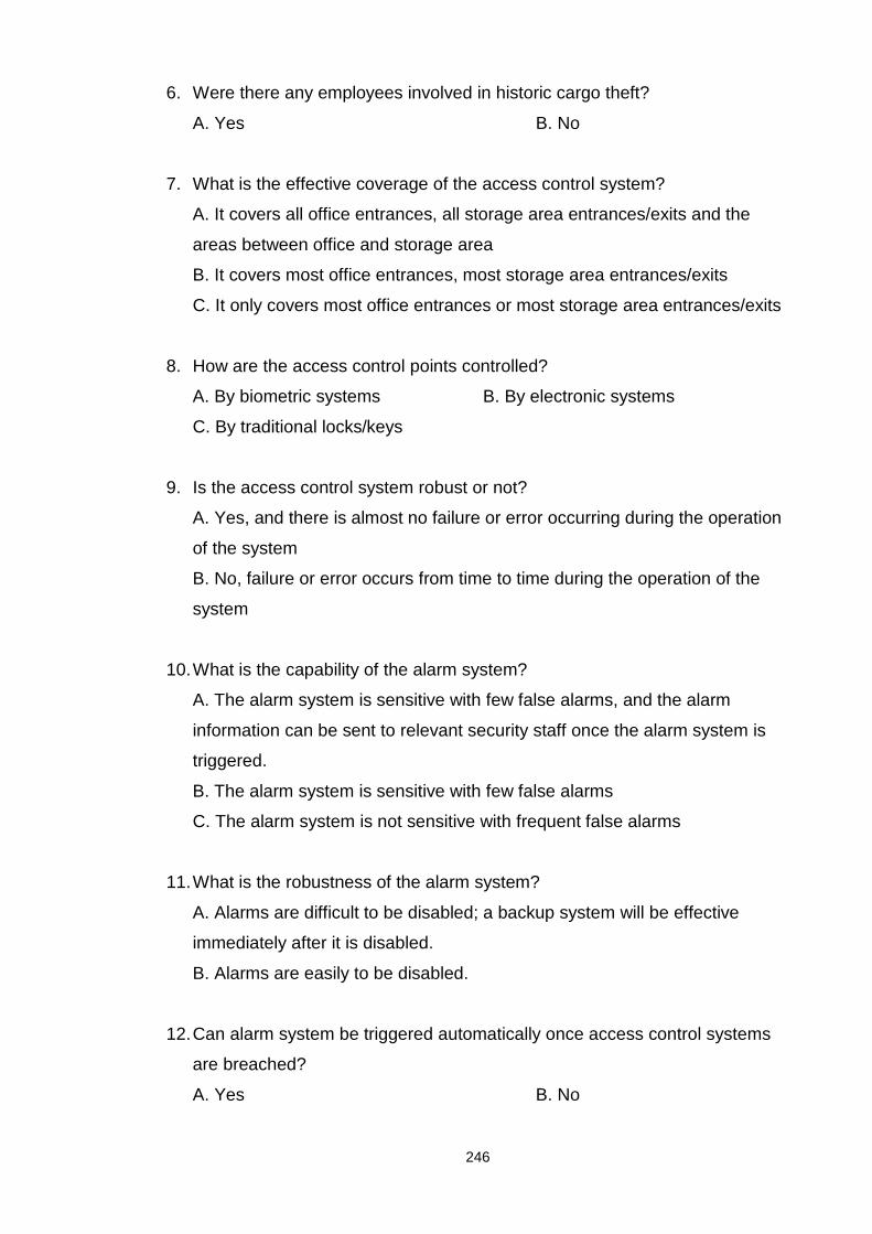
246
6. Were there any employees involved in historic cargo theft?
A. Yes B. No
7. What is the effective coverage of the access control system?
A. It covers all office entrances, all storage area entrances/exits and the
areas between office and storage area
B. It covers most office entrances, most storage area entrances/exits
C. It only covers most office entrances or most storage area entrances/exits
8. How are the access control points controlled?
A. By biometric systems B. By electronic systems
C. By traditional locks/keys
9. Is the access control system robust or not?
A. Yes, and there is almost no failure or error occurring during the operation
of the system
B. No, failure or error occurs from time to time during the operation of the
system
10. What is the capability of the alarm system?
A. The alarm system is sensitive with few false alarms, and the alarm
information can be sent to relevant security staff once the alarm system is
triggered.
B. The alarm system is sensitive with few false alarms
C. The alarm system is not sensitive with frequent false alarms
11. What is the robustness of the alarm system?
A. Alarms are difficult to be disabled; a backup system will be effective
immediately after it is disabled.
B. Alarms are easily to be disabled.
12. Can alarm system be triggered automatically once access control systems
are breached?
A. Yes B. No
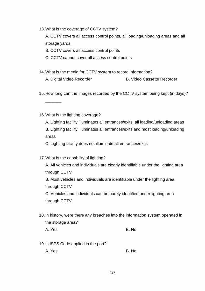
247
13. What is the coverage of CCTV system?
A. CCTV covers all access control points, all loading/unloading areas and all
storage yards.
B. CCTV covers all access control points
C. CCTV cannot cover all access control points
14. What is the media for CCTV system to record information?
A. Digital Video Recorder B. Video Cassette Recorder
15. How long can the images recorded by the CCTV system being kept (in days)?
_______
16. What is the lighting coverage?
A. Lighting facility illuminates all entrances/exits, all loading/unloading areas
B. Lighting facility illuminates all entrances/exits and most loading/unloading
areas
C. Lighting facility does not illuminate all entrances/exits
17. What is the capability of lighting?
A. All vehicles and individuals are clearly identifiable under the lighting area
through CCTV
B. Most vehicles and individuals are identifiable under the lighting area
through CCTV
C. Vehicles and individuals can be barely identified under lighting area
through CCTV
18. In history, were there any breaches into the information system operated in
the storage area?
A. Yes B. No
19. Is ISPS Code applied in the port?
A. Yes B. No

248
20. Are there any regulations developed to create and maintain security culture
in the port?
A. Yes, there is a set of regulations developed to create and maintain
security culture, and most employees can realize the importance of security
for the operation in the port
B. Yes, there is a set of regulations developed to create and maintain
security culture, however, only few employees realize the importance of
security for the operation in the port
C. No, there is no regulation developed to create or maintain security culture
21. Are the access control regulations considering the access control of current
employees?
A. Yes B. No
22. Are the access control regulations considering the access control of
terminated employees?
A. Yes B. No
23. Are the access control regulations considering the access control of visitors?
A. Yes B. No
24. Are there any regulations on stuffing and loading/unloading procedures?
A. Yes B. No
25. Are there any regulations on the process of timely reporting security incident?
A. Yes B. No
26. Is the execution status of regulations monitored?
A. Yes B. No
27. Is the execution status of regulations audited?
A. Yes B. No
28. Are the regulations updated regularly and when necessary?

249
A. Yes B. No
29. What is the status of application of Photo-ID Badge?
A. All employees and contractors are issued with a photo-ID badge
B. Not all employees and contractors are issued with a photo-ID badge
C. No photo-ID badge is applied.
30. What is the status of key/key card control?
A. Keys/Key Cards are strictly controlled, including the control of keys/key
cards of terminated employees
B. Keys/Key Cards are strictly controlled only for current employees
C. Keys/Key Cards are not strictly controlled
31. Are the following issues covered by the training towards employees: security
awareness, techniques to maintain the security and techniques to respond
to security incidents?
A. All the 3 issues are covered B. Some of the 3 issues are covered
C. None of the 3 issues are covered
32. Are there any background checks and periodic audit of employees?
A. Yes, the background of employees (within 5 years) are checked and
periodically audited.
B. Yes, the background of employees (within 5 years) are checked but not
periodically audited
C. No, there is no check on the background of employees.
33. Are there any logs for the operation of alarm system?
A. Yes B. No
34. Are there any logs for the operation of access control system?
A. Yes B. No
35. Is there a record for emergency contact?
A. Yes B. No
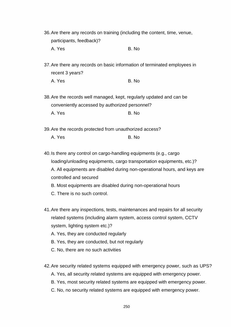
250
36. Are there any records on training (including the content, time, venue,
participants, feedback)?
A. Yes B. No
37. Are there any records on basic information of terminated employees in
recent 3 years?
A. Yes B. No
38. Are the records well managed, kept, regularly updated and can be
conveniently accessed by authorized personnel?
A. Yes B. No
39. Are the records protected from unauthorized access?
A. Yes B. No
40. Is there any control on cargo-handling equipments (e.g., cargo
loading/unloading equipments, cargo transportation equipments, etc.)?
A. All equipments are disabled during non-operational hours, and keys are
controlled and secured
B. Most equipments are disabled during non-operational hours
C. There is no such control.
41. Are there any inspections, tests, maintenances and repairs for all security
related systems (including alarm system, access control system, CCTV
system, lighting system etc.)?
A. Yes, they are conducted regularly
B. Yes, they are conducted, but not regularly
C. No, there are no such activities
42. Are security related systems equipped with emergency power, such as UPS?
A. Yes, all security related systems are equipped with emergency power.
B. Yes, most security related systems are equipped with emergency power.
C. No, no security related systems are equipped with emergency power.
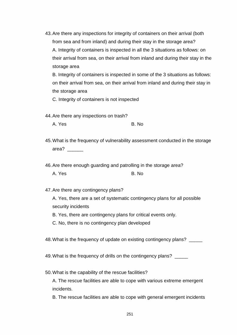
251
43. Are there any inspections for integrity of containers on their arrival (both
from sea and from inland) and during their stay in the storage area?
A. Integrity of containers is inspected in all the 3 situations as follows: on
their arrival from sea, on their arrival from inland and during their stay in the
storage area
B. Integrity of containers is inspected in some of the 3 situations as follows:
on their arrival from sea, on their arrival from inland and during their stay in
the storage area
C. Integrity of containers is not inspected
44. Are there any inspections on trash?
A. Yes B. No
45. What is the frequency of vulnerability assessment conducted in the storage
area? ______
46. Are there enough guarding and patrolling in the storage area?
A. Yes B. No
47. Are there any contingency plans?
A. Yes, there are a set of systematic contingency plans for all possible
security incidents
B. Yes, there are contingency plans for critical events only.
C. No, there is no contingency plan developed
48. What is the frequency of update on existing contingency plans? _____
49. What is the frequency of drills on the contingency plans? _____
50. What is the capability of the rescue facilities?
A. The rescue facilities are able to cope with various extreme emergent
incidents.
B. The rescue facilities are able to cope with general emergent incidents

252
C. The rescue facilities are not able to cope with general emergent incidents
51. Are rescue facilities conveniently accessible in case of emergency?
A. Yes B. No
52. Does the storage area have its own communication systems (e.g.,
interphone) besides public communication systems (e.g., telephone, cell
phone) in case of emergency?
A. Yes B. No
53. Are there any recovery plans?
A. Yes, There are a set of recovery plans and they are regularly updated
and drilled.
B. Recovery plans are not updated and drilled, or there is no recovery plans
54. According to the cargo stored in the port (e.g., whether the cargo listed in
IMDG Code stored in the storage area?), the environment of the port and
the historic cargo theft in the port, will there be any human loss due to cargo
theft in the port?
A. Yes, there may be human deaths caused by cargo theft in the port
B. Yes, there may be human injuries but no human caused by cargo in the
port
C. No, there will be no human loss caused by cargo theft in the port
55. According to the cargo stored in the port and the historic cargo theft in the
port, what is the potential financial loss due to cargo theft in the port?
A. More than 10,000 dollars
B. Below 10,000 dollars, but not negligible
C. Negligible
56. According to the cargo stored in the port, the partners of the port along the
CLSC, and the historic cargo theft in the port, will there be any reputational
loss if cargo theft happens in the port?
A. Yes B. No, negligible

253
57. According to the cargo stored in the port, the partners of the port along the
CLSC and the historic cargo theft in the port, what is the potential economic
loss due to cargo theft in the port?
A. More than 10,000 dollars
B. Below 10,000 dollars, but not negligible
C. Negligible
58. According to the cargo stored in the port, the environment of the port and the
historic cargo theft in the port, will the environment be impacted if cargo theft
happens in the port?
A. Yes B. No
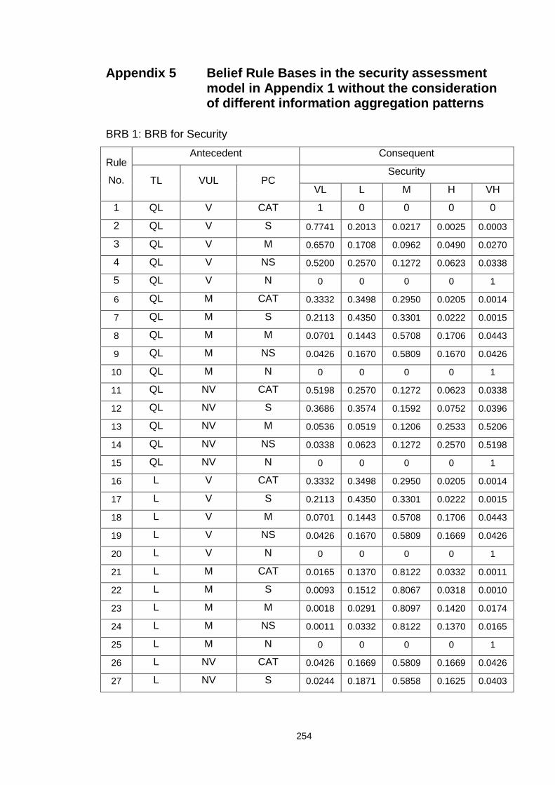
254
Appendix 5 Belief Rule Bases in the security assess ment model in Appendix 1 without the consideration of different information aggregation patterns
BRB 1: BRB for Security
Rule
No.
Antecedent Consequent
TL VUL PC Security
VL L M H VH
1 QL V CAT 1 0 0 0 0
2 QL V S 0.7741 0.2013 0.0217 0.0025 0.0003
3 QL V M 0.6570 0.1708 0.0962 0.0490 0.0270
4 QL V NS 0.5200 0.2570 0.1272 0.0623 0.0338
5 QL V N 0 0 0 0 1
6 QL M CAT 0.3332 0.3498 0.2950 0.0205 0.0014
7 QL M S 0.2113 0.4350 0.3301 0.0222 0.0015
8 QL M M 0.0701 0.1443 0.5708 0.1706 0.0443
9 QL M NS 0.0426 0.1670 0.5809 0.1670 0.0426
10 QL M N 0 0 0 0 1
11 QL NV CAT 0.5198 0.2570 0.1272 0.0623 0.0338
12 QL NV S 0.3686 0.3574 0.1592 0.0752 0.0396
13 QL NV M 0.0536 0.0519 0.1206 0.2533 0.5206
14 QL NV NS 0.0338 0.0623 0.1272 0.2570 0.5198
15 QL NV N 0 0 0 0 1
16 L V CAT 0.3332 0.3498 0.2950 0.0205 0.0014
17 L V S 0.2113 0.4350 0.3301 0.0222 0.0015
18 L V M 0.0701 0.1443 0.5708 0.1706 0.0443
19 L V NS 0.0426 0.1670 0.5809 0.1669 0.0426
20 L V N 0 0 0 0 1
21 L M CAT 0.0165 0.1370 0.8122 0.0332 0.0011
22 L M S 0.0093 0.1512 0.8067 0.0318 0.0010
23 L M M 0.0018 0.0291 0.8097 0.1420 0.0174
24 L M NS 0.0011 0.0332 0.8122 0.1370 0.0165
25 L M N 0 0 0 0 1
26 L NV CAT 0.0426 0.1669 0.5809 0.1669 0.0426
27 L NV S 0.0244 0.1871 0.5858 0.1625 0.0403

255
28 L NV M 0.0023 0.0175 0.2861 0.3528 0.3414
29 L NV NS 0.0014 0.0205 0.2950 0.3500 0.3332
30 L NV N 0 0 0 0 1
31 NL V CAT 0.5200 0.2570 0.1272 0.0623 0.0338
32 NL V S 0.3686 0.3574 0.1592 0.0752 0.0396
33 NL V M 0.0536 0.0519 0.1206 0.2533 0.5206
34 NL V NS 0.0338 0.0623 0.1272 0.2570 0.5198
35 NL V N 0 0 0 0 1
36 NL M CAT 0.0426 0.1669 0.5809 0.1669 0.0426
37 NL M S 0.0244 0.1871 0.5858 0.1625 0.0403
38 NL M M 0.0023 0.0175 0.2861 0.3528 0.3414
39 NL M NS 0.0014 0.0205 0.2950 0.3498 0.3332
40 NL M N 0 0 0 0 1
41 NL NV CAT 0.0338 0.0623 0.1272 0.2570 0.5198
42 NL NV S 0.0201 0.0728 0.1338 0.2608 0.5124
43 NL NV M 0.0004 0.0014 0.0131 0.1137 0.8714
44 NL NV NS 0.0002 0.0016 0.0138 0.1152 0.8691
45 NL NV N 0 0 0 0 1
46 N V CAT 0 0 0 0 1
47 N V S 0 0 0 0 1
48 N V M 0 0 0 0 1
49 N V NS 0 0 0 0 1
50 N V N 0 0 0 0 1
51 N M CAT 0 0 0 0 1
52 N M S 0 0 0 0 1
53 N M M 0 0 0 0 1
54 N M NS 0 0 0 0 1
55 N M N 0 0 0 0 1
56 N NV CAT 0 0 0 0 1
57 N NV S 0 0 0 0 1
58 N NV M 0 0 0 0 1
59 N NV NS 0 0 0 0 1
60 N NV N 0 0 0 0 1
TL: Threat Likelihood, VUL: Vulnerability, PC: Pote ntial Consequence
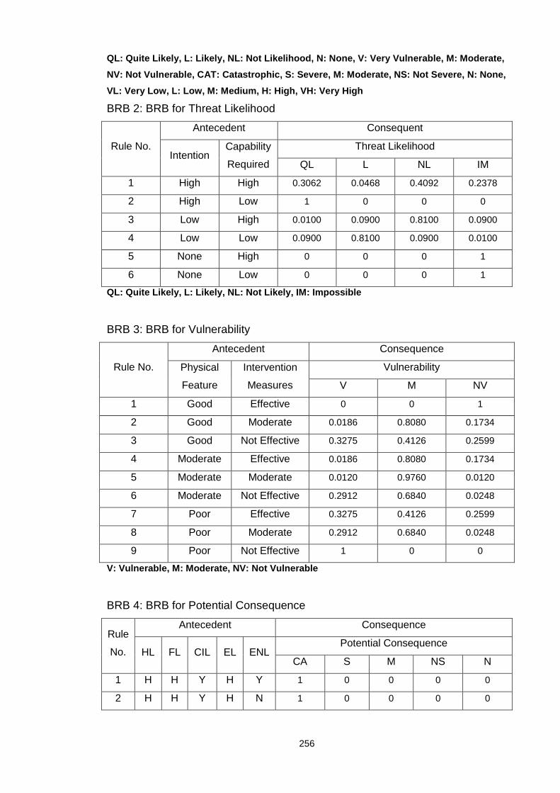
256
QL: Quite Likely, L: Likely, NL: Not Likelihood, N: None, V: Very Vulnerable, M: Moderate,
NV: Not Vulnerable, CAT: Catastrophic, S: Severe, M : Moderate, NS: Not Severe, N: None,
VL: Very Low, L: Low, M: Medium, H: High, VH: Very High
BRB 2: BRB for Threat Likelihood
Rule No.
Antecedent Consequent
Intention Capability
Required
Threat Likelihood
QL L NL IM
1 High High 0.3062 0.0468 0.4092 0.2378
2 High Low 1 0 0 0
3 Low High 0.0100 0.0900 0.8100 0.0900
4 Low Low 0.0900 0.8100 0.0900 0.0100
5 None High 0 0 0 1
6 None Low 0 0 0 1
QL: Quite Likely, L: Likely, NL: Not Likely, IM: Im possible
BRB 3: BRB for Vulnerability
Rule No.
Antecedent Consequence
Physical
Feature
Intervention
Measures
Vulnerability
V M NV
1 Good Effective 0 0 1
2 Good Moderate 0.0186 0.8080 0.1734
3 Good Not Effective 0.3275 0.4126 0.2599
4 Moderate Effective 0.0186 0.8080 0.1734
5 Moderate Moderate 0.0120 0.9760 0.0120
6 Moderate Not Effective 0.2912 0.6840 0.0248
7 Poor Effective 0.3275 0.4126 0.2599
8 Poor Moderate 0.2912 0.6840 0.0248
9 Poor Not Effective 1 0 0
V: Vulnerable, M: Moderate, NV: Not Vulnerable
BRB 4: BRB for Potential Consequence
Rule
No.
Antecedent Consequence
HL FL CIL EL ENL Potential Consequence
CA S M NS N
1 H H Y H Y 1 0 0 0 0
2 H H Y H N 1 0 0 0 0

257
3 H H Y L Y 1 0 0 0 0
4 H H Y L N 1 0 0 0 0
5 H H Y N Y 1 0 0 0 0
6 H H Y N N 1 0 0 0 0
7 H H N H Y 1 0 0 0 0
8 H H N H N 1 0 0 0 0
9 H H N L Y 1 0 0 0 0
10 H H N L N 1 0 0 0 0
11 H H N N Y 1 0 0 0 0
12 H H N N N 1 0 0 0 0
13 H L Y H Y 1 0 0 0 0
14 H L Y H N 1 0 0 0 0
15 H L Y L Y 1 0 0 0 0
16 H L Y L N 1 0 0 0 0
17 H L Y N Y 1 0 0 0 0
18 H L Y N N 1 0 0 0 0
19 H L N H Y 1 0 0 0 0
20 H L N H N 1 0 0 0 0
21 H L N L Y 1 0 0 0 0
22 H L N L N 1 0 0 0 0
23 H L N N Y 1 0 0 0 0
24 H L N N N 1 0 0 0 0
25 H N Y H Y 1 0 0 0 0
26 H N Y H N 1 0 0 0 0
27 H N Y L Y 1 0 0 0 0
28 H N Y L N 1 0 0 0 0
29 H N Y N Y 1 0 0 0 0
30 H N Y N N 1 0 0 0 0
31 H N N H Y 1 0 0 0 0
32 H N N H N 1 0 0 0 0
33 H N N L Y 1 0 0 0 0
34 H N N L N 1 0 0 0 0
35 H N N N Y 1 0 0 0 0
36 H N N N N 1 0 0 0 0
37 L H Y H Y 0.3141 0.4833 0.1427 0.0581 0.0019

258
38 L H Y H N 0.5405 0.3693 0.0765 0.0064 0.0072
39 L H Y L Y 0.1194 0.0975 0.1739 0.6010 0.0081
40 L H Y L N 0.4361 0.1582 0.1981 0.1414 0.0662
41 L H Y N Y 0.4361 0.1582 0.1981 0.1414 0.0662
42 L H Y N N 0.6015 0.0969 0.0852 0.0126 0.2039
43 L H N H Y 0.3517 0.4953 0.0594 0.0596 0.0340
44 L H N H N 0.5249 0.3283 0.0277 0.0057 0.1134
45 L H N L Y 0.1249 0.0934 0.0677 0.5755 0.1385
46 L H N L N 0.2340 0.0777 0.0395 0.0694 0.5793
47 L H N N Y 0.2340 0.0777 0.0395 0.0694 0.5793
48 L H N N N 0.1482 0.0219 0.0078 0.0028 0.8193
49 L L Y H Y 0.0820 0.3589 0.4361 0.1199 0.0031
50 L L Y H N 0.2091 0.4067 0.3469 0.0197 0.0176
51 L L Y L Y 0.0165 0.0383 0.2815 0.6565 0.0071
52 L L Y L N 0.0919 0.0949 0.4891 0.2356 0.0885
53 L L Y N Y 0.0919 0.0949 0.4891 0.2356 0.0885
54 L L Y N N 0.1841 0.0844 0.3054 0.0304 0.3956
55 L L N H Y 0.1119 0.4484 0.2214 0.1498 0.0686
56 L L N H N 0.2061 0.3668 0.1272 0.0178 0.2822
57 L L N L Y 0.0189 0.0402 0.1199 0.6882 0.1328
58 L L N L N 0.0455 0.0430 0.0901 0.1068 0.7145
59 L L N N Y 0.0455 0.0430 0.0901 0.1068 0.7145
60 L L N N N 0.0269 0.0113 0.0166 0.0041 0.9412
61 L N Y H Y 0.1119 0.4484 0.2214 0.1498 0.0686
62 L N Y H N 0.2061 0.3668 0.1272 0.0178 0.2822
63 L N Y L Y 0.0189 0.0402 0.1199 0.6882 0.1328
64 L N Y L N 0.0455 0.0430 0.0901 0.1068 0.7145
65 L N Y N Y 0.0456 0.0430 0.0901 0.1068 0.7145
66 L N Y N N 0.0269 0.0113 0.0166 0.0041 0.9412
67 L N N H Y 0.0601 0.2205 0.0443 0.0737 0.6014
68 L N N H N 0.0396 0.0645 0.0091 0.0031 0.8838
69 L N N L Y 0.0065 0.0127 0.0154 0.2176 0.7478
70 L N N L N 0.0038 0.0033 0.0028 0.0082 0.9818
71 L N N N Y 0.0038 0.0033 0.0028 0.0082 0.9818
72 L N N N N 0.0017 0.0007 0.0004 0.0002 0.9969

259
73 N H Y H Y 0.1119 0.4484 0.2214 0.1498 0.0686
74 N H Y H N 0.2061 0.3668 0.1272 0.0178 0.2822
75 N H Y L Y 0.0189 0.0402 0.1199 0.6882 0.1328
76 N H Y L N 0.0455 0.0430 0.0901 0.1068 0.7145
77 N H Y N Y 0.0455 0.0430 0.0901 0.1068 0.7145
78 N H Y N N 0.0269 0.0113 0.0166 0.0041 0.9412
79 N H N H Y 0.0601 0.2205 0.0443 0.0737 0.6014
80 N H N H N 0.0396 0.0644 0.0091 0.0031 0.8838
81 N H N L Y 0.0065 0.0127 0.0154 0.2176 0.7478
82 N H N L N 0.0038 0.0033 0.0028 0.0083 0.9818
83 N H N N Y 0.0038 0.0033 0.0028 0.0082 0.9818
84 N H N N N 0.0017 0.0007 0.0004 0.0002 0.9969
85 N L Y H Y 0.0200 0.2278 0.4631 0.2115 0.0777
86 N L Y H N 0.0441 0.2235 0.3190 0.0301 0.3832
87 N L Y L Y 0.0024 0.0146 0.1796 0.6957 0.1076
88 N L Y L N 0.0069 0.0186 0.1600 0.1280 0.6865
89 N L Y N Y 0.0069 0.0186 0.1600 0.1280 0.6865
90 N L Y N N 0.0043 0.0051 0.0311 0.0051 0.9544
91 N L N H Y 0.0107 0.1120 0.0926 0.1040 0.6806
92 N L N H N 0.0066 0.0308 0.0179 0.0041 0.9406
93 N L N L Y 0.0010 0.0054 0.0270 0.2574 0.7092
94 N L N L N 0.0006 0.0015 0.0052 0.0103 0.9824
95 N L N N Y 0.0006 0.0015 0.0052 0.0103 0.9824
96 N L N N N 0.0003 0.0003 0.0007 0.0003 0.9984
97 N N Y H Y 0.0107 0.1121 0.0926 0.1040 0.6806
98 N N Y H N 0.0066 0.0308 0.0179 0.0041 0.9406
99 N N Y L Y 0.0010 0.0054 0.0270 0.2574 0.7092
100 N N Y L N 0.0006 0.0015 0.0052 0.0103 0.9824
101 N N Y N Y 0.0006 0.0015 0.0052 0.0103 0.9824
102 N N Y N N 0.0003 0.0003 0.0007 0.0003 0.9984
103 N N N H Y 0.0009 0.0090 0.0030 0.0084 0.9786
104 N N N H N 0.0004 0.0018 0.0004 0.0002 0.9971
105 N N N L Y 0.0000 0.0004 0.0009 0.01994 0.9787
106 N N N L N 0.0000 0.0000 0.0001 0.0006 0.9992
107 N N N N Y 0.0000 0.0000 0.0001 0.0006 0.9992

260
108 N N N N N 0 0 0 0 1
HL: Human Loss, FL: Financial Loss, CIL: Cooperate Image Loss, EL: Economic Loss,
ENL: Environmental Loss
H: High, L: Low, N: None, Y: Yes, N: No, CAT: Catas trophic, S: Severe, M: Moderate, NS:
Not Severe, N: None
BRB 5: BRB for Capability Required
Rule No.
Antecedent Consequence
Preventative
Capability
Cargo
Magnitude
Capability Required
High Low
1 High Big 1 0
2 High Small 0.1818 0.8182
3 Low Big 0.5625 0.4375
4 Low Small 0 1
BRB 6: BRB for Physical Feature
Rule No.
Antecedent Consequence
Historic
Features
Employee
Features
Facility
Features
Physical Feature
Good Moderate Poor
1 Good Good Good 1 0 0
2 Good Good Moderate 0.8440 0.1426 0.0134
3 Good Good Poor 0.7900 0.0734 0.1366
4 Good Poor Good 0.7375 0.1773 0.0852
5 Good Poor Moderate 0.1799 0.6263 0.1938
6 Good Poor Poor 0.0682 0.1307 0.8011
7 Moderate Good Good 0.9034 0.0843 0.0123
8 Moderate Good Moderate 0.4035 0.5453 0.0512
9 Moderate Good Poor 0.3198 0.2379 0.4423
10 Moderate Poor Good 0.2600 0.4998 0.2403
11 Moderate Poor Moderate 0.0267 0.7433 0.2300
12 Moderate Poor Poor 0.0091 0.1390 0.8520
13 Poor Good Good 0.7497 0.1624 0.0879
14 Poor Good Moderate 0.1912 0.5998 0.2090
15 Poor Good Poor 0.0683 0.1179 0.8138
16 Poor Poor Good 0.0745 0.3323 0.5932
17 Poor Poor Moderate 0.0071 0.4620 0.5309
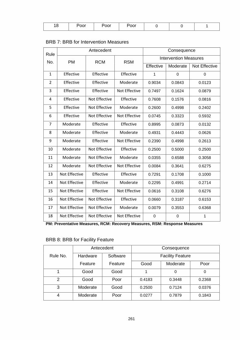
261
18 Poor Poor Poor 0 0 1
BRB 7: BRB for Intervention Measures
Rule
No.
Antecedent Consequence
PM RCM RSM Intervention Measures
Effective Moderate Not Effective
1 Effective Effective Effective 1 0 0
2 Effective Effective Moderate 0.9034 0.0843 0.0123
3 Effective Effective Not Effective 0.7497 0.1624 0.0879
4 Effective Not Effective Effective 0.7608 0.1576 0.0816
5 Effective Not Effective Moderate 0.2600 0.4998 0.2402
6 Effective Not Effective Not Effective 0.0745 0.3323 0.5932
7 Moderate Effective Effective 0.8995 0.0873 0.0132
8 Moderate Effective Moderate 0.4931 0.4443 0.0626
9 Moderate Effective Not Effective 0.2390 0.4998 0.2613
10 Moderate Not Effective Effective 0.2500 0.5000 0.2500
11 Moderate Not Effective Moderate 0.0355 0.6588 0.3058
12 Moderate Not Effective Not Effective 0.0084 0.3641 0.6275
13 Not Effective Effective Effective 0.7291 0.1708 0.1000
14 Not Effective Effective Moderate 0.2295 0.4991 0.2714
15 Not Effective Effective Not Effective 0.0616 0.3108 0.6276
16 Not Effective Not Effective Effective 0.0660 0.3187 0.6153
17 Not Effective Not Effective Moderate 0.0079 0.3553 0.6368
18 Not Effective Not Effective Not Effective 0 0 1
PM: Preventative Measures, RCM: Recovery Measures, RSM: Response Measures
BRB 8: BRB for Facility Feature
Rule No.
Antecedent Consequence
Hardware
Feature
Software
Feature
Facility Feature
Good Moderate Poor
1 Good Good 1 0 0
2 Good Poor 0.4183 0.3448 0.2368
3 Moderate Good 0.2500 0.7124 0.0376
4 Moderate Poor 0.0277 0.7879 0.1843
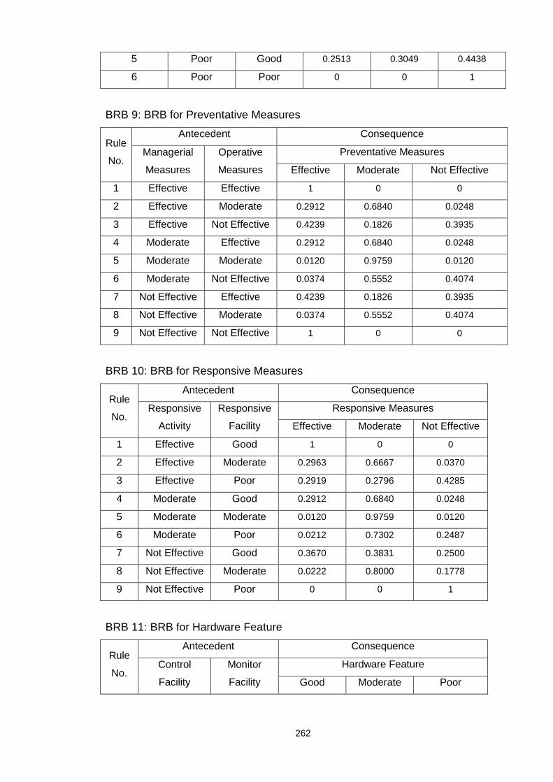
262
5 Poor Good 0.2513 0.3049 0.4438
6 Poor Poor 0 0 1
BRB 9: BRB for Preventative Measures
Rule
No.
Antecedent Consequence
Managerial
Measures
Operative
Measures
Preventative Measures
Effective Moderate Not Effective
1 Effective Effective 1 0 0
2 Effective Moderate 0.2912 0.6840 0.0248
3 Effective Not Effective 0.4239 0.1826 0.3935
4 Moderate Effective 0.2912 0.6840 0.0248
5 Moderate Moderate 0.0120 0.9759 0.0120
6 Moderate Not Effective 0.0374 0.5552 0.4074
7 Not Effective Effective 0.4239 0.1826 0.3935
8 Not Effective Moderate 0.0374 0.5552 0.4074
9 Not Effective Not Effective 1 0 0
BRB 10: BRB for Responsive Measures
Rule
No.
Antecedent Consequence
Responsive
Activity
Responsive
Facility
Responsive Measures
Effective Moderate Not Effective
1 Effective Good 1 0 0
2 Effective Moderate 0.2963 0.6667 0.0370
3 Effective Poor 0.2919 0.2796 0.4285
4 Moderate Good 0.2912 0.6840 0.0248
5 Moderate Moderate 0.0120 0.9759 0.0120
6 Moderate Poor 0.0212 0.7302 0.2487
7 Not Effective Good 0.3670 0.3831 0.2500
8 Not Effective Moderate 0.0222 0.8000 0.1778
9 Not Effective Poor 0 0 1
BRB 11: BRB for Hardware Feature
Rule
No.
Antecedent Consequence
Control
Facility
Monitor
Facility
Hardware Feature
Good Moderate Poor

263
1 Good Good 1 0 0
2 Good Moderate 0.3365 0.6274 0.0361
3 Good Poor 0.3982 0.1362 0.4657
4 Moderate Good 0.3365 0.6274 0.0361
5 Moderate Moderate 0.0120 0.9759 0.0120
6 Moderate Poor 0.0374 0.5552 0.4074
7 Poor Good 0.3982 0.1362 0.4657
8 Poor Moderate 0.0374 0.5552 0.4074
9 Poor Poor 0 0 1
BRB 12: BRB for Managerial Measures
Rule
No.
Antecedent Consequence
RE MR Managerial Measures
Effective Moderate Not Effective
1 Effective Effective 1 0 0
2 Effective Moderate 0.5353 0.4191 0.0456
3 Effective Not Effective 0.4568 0.3366 0.2067
4 Moderate Effective 0.3379 0.5985 0.0636
5 Moderate Moderate 0.0588 0.8823 0.0588
6 Moderate Not Effective 0.0490 0.6910 0.2601
7 Not Effective Effective 0.2971 0.2189 0.4839
8 Not Effective Moderate 0.0629 0.3926 0.5445
9 Not Effective Not Effective 0 0 1
RE: Regulations, MR: Management on Regulations
BRB 13: BRB for Operative Measures
Rule
No.
Antecedent Consequence
OAC OTA ORE OSE OOI Operative Measures
E M NE
1 E E E E E 1 0 0
2 E E E E NE 0.9819 0.0175 0.0006
3 E E E NE E 0.9819 0.0175 0.0006
4 E E E NE NE 0.7429 0.1939 0.0633
5 E E NE E E 0.9819 0.0175 0.0006
6 E E NE E NE 0.7429 0.1939 0.0633

264
7 E E NE NE E 0.7429 0.1939 0.0633
8 E E NE NE NE 0.0603 0.2311 0.7085
9 E NE E E E 0.9819 0.0175 0.0006
10 E NE E E NE 0.7429 0.1939 0.0633
11 E NE E NE E 0.7429 0.1939 0.0633
12 E NE E NE NE 0.0603 0.2311 0.7085
13 E NE NE E E 0.7429 0.1939 0.0633
14 E NE NE E NE 0.0603 0.2311 0.7085
15 E NE NE NE E 0.0603 0.2311 0.7085
16 E NE NE NE NE 0.0006 0.0335 0.9659
17 NE E E E E 0.9819 0.0175 0.0006
18 NE E E E NE 0.7429 0.1939 0.0633
19 NE E E NE E 0.7429 0.1939 0.0633
20 NE E E NE NE 0.0603 0.2311 0.7085
21 NE E NE E E 0.7429 0.1939 0.0633
22 NE E NE E NE 0.0603 0.2311 0.7085
23 NE E NE NE E 0.0603 0.2311 0.7085
24 NE E NE NE NE 0.0006 0.0335 0.9659
25 NE NE E E E 0.7429 0.1939 0.0633
26 NE NE E E NE 0.0603 0.2311 0.7085
27 NE NE E NE E 0.0603 0.2311 0.7085
28 NE NE E NE NE 0.0006 0.0335 0.9659
29 NE NE NE E E 0.0603 0.2311 0.7085
30 NE NE NE E NE 0.0006 0.0335 0.9659
31 NE NE NE NE E 0.0006 0.0335 0.9659
32 NE NE NE NE NE 0 0 1
OAC: Operations regarding Access Control, OTA: Oper ations regarding Employee
Training/Auditing, ORE: Operations regarding Record s, OSE: Operations regarding
Security related Equipments, OOI: Operations regard ing Other Issues
E: Effective, NE: Not Effective, M: Moderate
BRB 14: BRB for Responsive Activity
Rule No.
Antecedent Consequence
DCP UCP DRCP Responsive Activity
E M NE
1 Good Good Good 1 0 0

265
2 Good Good Moderate 0.8569 0.1258 0.0173
3 Good Good Poor 0.7670 0.1388 0.0942
4 Good Moderate Good 0.8569 0.1258 0.0173
5 Good Moderate Moderate 0.5166 0.4280 0.0554
6 Good Moderate Poor 0.3739 0.3821 0.2440
7 Good Poor Good 0.7670 0.1388 0.0942
8 Good Poor Moderate 0.3739 0.3821 0.2440
9 Good Poor Poor 0.1606 0.2023 0.6372
10 Moderate Good Good 0.4620 0.5217 0.0164
11 Moderate Good Moderate 0.1322 0.8429 0.0249
12 Moderate Good Poor 0.1000 0.7857 0.1144
13 Moderate Moderate Good 0.1322 0.8429 0.0249
14 Moderate Moderate Moderate 0.0263 0.9474 0.0263
15 Moderate Moderate Poor 0.0194 0.8624 0.1182
16 Moderate Poor Good 0.1000 0.7857 0.1144
17 Moderate Poor Moderate 0.0194 0.8624 0.1182
18 Moderate Poor Poor 0.0108 0.5903 0.3989
19 Poor Good Good 0.5166 0.3129 0.1706
20 Poor Good Moderate 0.1620 0.5539 0.2841
21 Poor Good Poor 0.0629 0.2654 0.6716
22 Poor Moderate Good 0.1620 0.5539 0.2841
23 Poor Moderate Moderate 0.0337 0.6517 0.3146
24 Poor Moderate Poor 0.0123 0.2921 0.6956
25 Poor Poor Good 0.0629 0.2654 0.6716
26 Poor Poor Moderate 0.0123 0.2921 0.6956
27 Poor Poor Poor 0 0 1
DCP: Development of Contingency Plan, UCP: Update o f Contingency Plan, DRCP: Drill
of Contingency Plan
E: Effective, M: Moderate, NE: Not Effective
BRB 15: BRB for Responsive Facility
Rule No.
Antecedent Consequence
Rescue
Facility
Communication
Facility
Responsive Facility
Good Moderate Poor
1 Good Good 1 0 0
2 Good Poor 0.3333 0.3333 0.3334

266
3 Moderate Good 0.3365 0.6274 0.0361
4 Moderate Poor 0.0186 0.8080 0.1734
5 Poor Good 0.3333 0.3333 0.3334
6 Poor Poor 0 0 1
BRB 16: BRB for Control Facility
Rule No.
Antecedent Consequence
ACS CON AS Control Facility
Good Moderate Poor
1 Good Yes Good 1 0 0
2 Good Yes Moderate 0.6765 0.3127 0.0108
3 Good Yes Poor 0.6483 0.2297 0.1220
4 Good No Good 0.8125 0.1562 0.0313
5 Good No Moderate 0.1946 0.7172 0.0881
6 Good No Poor 0.1095 0.3090 0.5816
7 Moderate Yes Good 0.6765 0.3127 0.0108
8 Moderate Yes Moderate 0.0996 0.8817 0.0187
9 Moderate Yes Poor 0.1000 0.6788 0.2211
10 Moderate No Good 0.1947 0.7172 0.0881
11 Moderate No Moderate 0.0130 0.9179 0.0691
12 Moderate No Poor 0.0085 0.4603 0.5311
13 Poor Yes Good 0.6483 0.2297 0.1220
14 Poor Yes Moderate 0.1000 0.6788 0.2211
15 Poor Yes Poor 0.0311 0.1617 0.8072
16 Poor No Good 0.1094 0.3090 0.5816
17 Poor No Moderate 0.0085 0.4603 0.5311
18 Poor No Poor 0 0 1
ACS: Access Control System, AS: Alarm System, CON: Connection between ACS and AS
BRB 17: BRB for Monitor Facility
Rule No.
Antecedent Consequence
CCTV
Facility
Lighting
Facility
Monitor Facility
Good Moderate Poor
1 Good Good 1 0 0
2 Good Moderate 0.3365 0.6274 0.0361
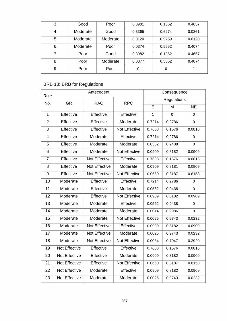
267
3 Good Poor 0.3981 0.1362 0.4657
4 Moderate Good 0.3365 0.6274 0.0361
5 Moderate Moderate 0.0120 0.9759 0.0120
6 Moderate Poor 0.0374 0.5552 0.4074
7 Poor Good 0.3982 0.1362 0.4657
8 Poor Moderate 0.0377 0.5552 0.4074
9 Poor Poor 0 0 1
BRB 18: BRB for Regulations
Rule
No.
Antecedent Consequence
GR RAC RPC Regulations
E M NE
1 Effective Effective Effective 1 0 0
2 Effective Effective Moderate 0.7214 0.2786 0
3 Effective Effective Not Effective 0.7608 0.1576 0.0816
4 Effective Moderate Effective 0.7214 0.2786 0
5 Effective Moderate Moderate 0.0562 0.9438 0
6 Effective Moderate Not Effective 0.0909 0.8182 0.0909
7 Effective Not Effective Effective 0.7608 0.1576 0.0816
8 Effective Not Effective Moderate 0.0909 0.8181 0.0909
9 Effective Not Effective Not Effective 0.0660 0.3187 0.6153
10 Moderate Effective Effective 0.7214 0.2786 0
11 Moderate Effective Moderate 0.0562 0.9438 0
12 Moderate Effective Not Effective 0.0909 0.8182 0.0909
13 Moderate Moderate Effective 0.0562 0.9438 0
14 Moderate Moderate Moderate 0.0014 0.9986 0
15 Moderate Moderate Not Effective 0.0025 0.9743 0.0232
16 Moderate Not Effective Effective 0.0909 0.8182 0.0909
17 Moderate Not Effective Moderate 0.0025 0.9743 0.0232
18 Moderate Not Effective Not Effective 0.0034 0.7047 0.2920
19 Not Effective Effective Effective 0.7608 0.1576 0.0816
20 Not Effective Effective Moderate 0.0909 0.8182 0.0909
21 Not Effective Effective Not Effective 0.0660 0.3187 0.6153
22 Not Effective Moderate Effective 0.0909 0.8182 0.0909
23 Not Effective Moderate Moderate 0.0025 0.9743 0.0232
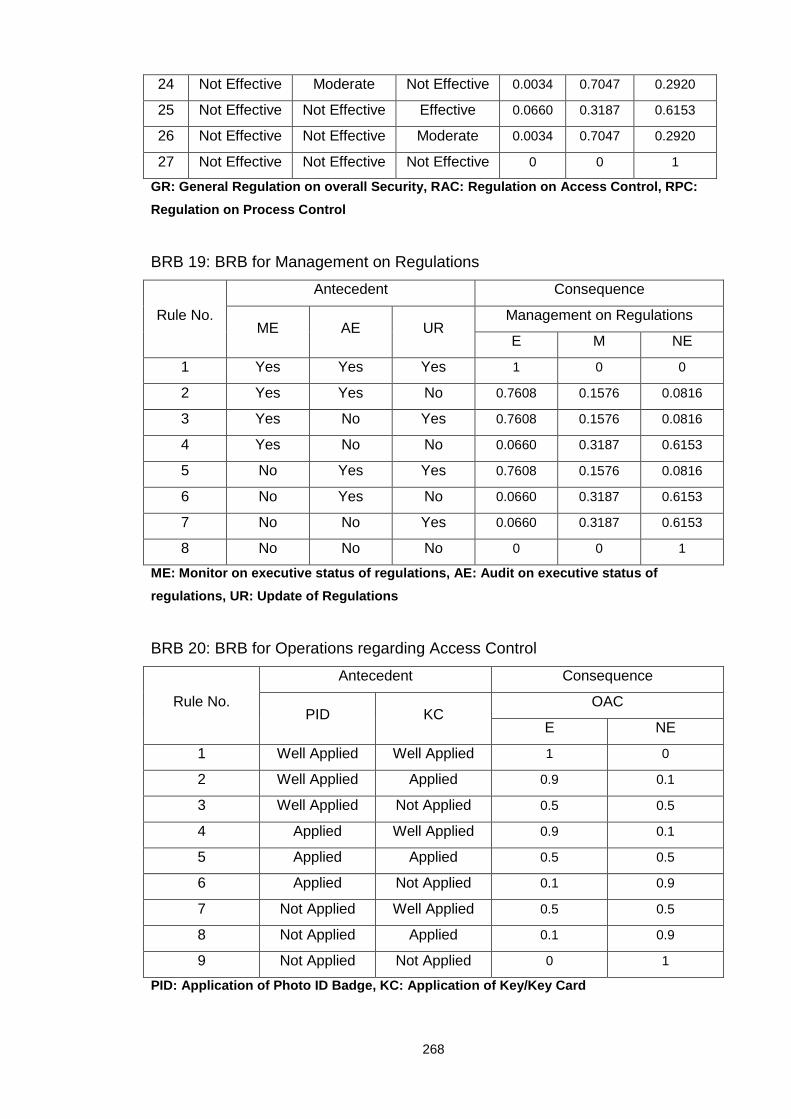
268
24 Not Effective Moderate Not Effective 0.0034 0.7047 0.2920
25 Not Effective Not Effective Effective 0.0660 0.3187 0.6153
26 Not Effective Not Effective Moderate 0.0034 0.7047 0.2920
27 Not Effective Not Effective Not Effective 0 0 1
GR: General Regulation on overall Security, RAC: Re gulation on Access Control, RPC:
Regulation on Process Control
BRB 19: BRB for Management on Regulations
Rule No.
Antecedent Consequence
ME AE UR Management on Regulations
E M NE
1 Yes Yes Yes 1 0 0
2 Yes Yes No 0.7608 0.1576 0.0816
3 Yes No Yes 0.7608 0.1576 0.0816
4 Yes No No 0.0660 0.3187 0.6153
5 No Yes Yes 0.7608 0.1576 0.0816
6 No Yes No 0.0660 0.3187 0.6153
7 No No Yes 0.0660 0.3187 0.6153
8 No No No 0 0 1
ME: Monitor on executive status of regulations, AE: Audit on executive status of
regulations, UR: Update of Regulations
BRB 20: BRB for Operations regarding Access Control
Rule No.
Antecedent Consequence
PID KC OAC
E NE
1 Well Applied Well Applied 1 0
2 Well Applied Applied 0.9 0.1
3 Well Applied Not Applied 0.5 0.5
4 Applied Well Applied 0.9 0.1
5 Applied Applied 0.5 0.5
6 Applied Not Applied 0.1 0.9
7 Not Applied Well Applied 0.5 0.5
8 Not Applied Applied 0.1 0.9
9 Not Applied Not Applied 0 1
PID: Application of Photo ID Badge, KC: Application of Key/Key Card

269
E: Effective, NE: Not Effective
BRB 21: BRB for Operations regarding Employee Training/Auditing
Rule No.
Antecedent Consequence
Training Auditing OTA
E NE
1 Good Good 1 0
2 Good Moderate 0.9 0.1
3 Good Poor 0.5 0.5
4 Moderate Good 0.9 0.1
5 Moderate Moderate 0.5 0.5
6 Moderate Poor 0.1 0.9
7 Poor Good 0.5 0.5
8 Poor Moderate 0.1 0.9
9 Poor Poor 0 1
OTA: Operations regarding Employee Training/Auditin g
E: Effective, NE: Not Effective
BRB 22: BRB for Operations regarding Records
Rule No.
Antecedent Consequence
Records Protection
on Records
Management
on Records
ORE
E NE
1 Yes Yes Well 1 0
2 Yes Yes Poor 0.9 0.1
3 Yes No Well 0.9 0.1
4 Yes No Poor 0.2647 0.7353
5 No Yes Well 0.7353 0.2647
6 No Yes Poor 0.1 0.9
7 No No Well 0.1 0.9
8 No No Poor 0 1
ORE: Operations regarding Records
E: Effective, NE: Not Effective
BRB 23: BRB for Operations regarding Security related Equipments
Rule No. Antecedent Consequence
CCH TMR UPS OSE

270
E NE
1 Good Good Good 1 0
2 Good Good Moderate 0.9878 0.0122
3 Good Good Poor 0.9 0.1
4 Good Moderate Good 0.9878 0.0122
5 Good Moderate Moderate 0.9 0.1
6 Good Moderate Poor 0.5 0.5
7 Good Poor Good 0.9 0.1
8 Good Poor Moderate 0.5 0.5
9 Good Poor Poor 0.1 0.9
10 Moderate Good Good 0.9878 0.0122
11 Moderate Good Moderate 0.9 0.1
12 Moderate Good Poor 0.5 0.5
13 Moderate Moderate Good 0.9 0.1
14 Moderate Moderate Moderate 0.5 0.5
15 Moderate Moderate Poor 0.1 0.9
16 Moderate Poor Good 0.5 0.5
17 Moderate Poor Moderate 0.1 0.9
18 Moderate Poor Poor 0.0122 0.9878
19 Poor Good Good 0.9 0.1
20 Poor Good Moderate 0.5 0.5
21 Poor Good Poor 0.1 0.9
22 Poor Moderate Good 0.5 0.5
23 Poor Moderate Moderate 0.1 0.9
24 Poor Moderate Poor 0.0122 0.9878
25 Poor Poor Good 0.1 0.9
26 Poor Poor Moderate 0.0122 0.9878
27 Poor Poor Poor 0 1
CCH: Control on cargo-handling equipments, TMR: Tes t/maintenance/repair for security
systems, UPS: UPS equipments on security systems, O SE: Operations regarding
Security related Equipments
E: Effective, NE: Not Effective
BRB 24: BRB for Operations regarding Other Issues
Rule No. Antecedent Consequence
CI VA GP OOI
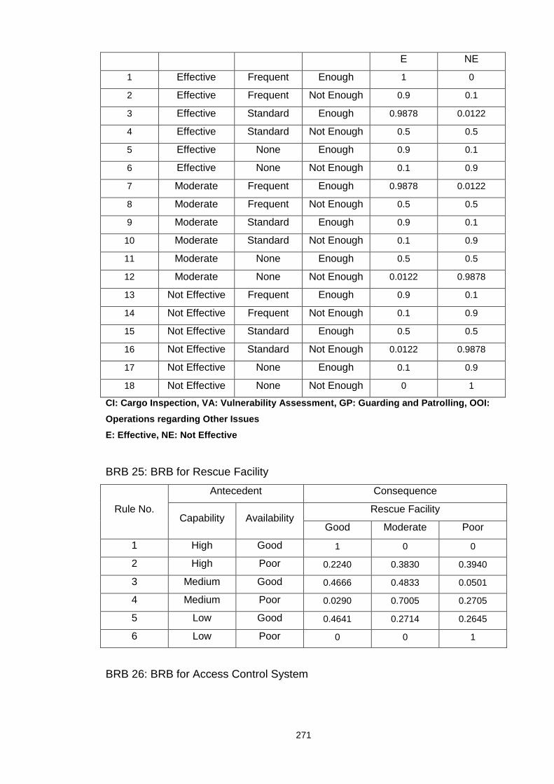
271
E NE
1 Effective Frequent Enough 1 0
2 Effective Frequent Not Enough 0.9 0.1
3 Effective Standard Enough 0.9878 0.0122
4 Effective Standard Not Enough 0.5 0.5
5 Effective None Enough 0.9 0.1
6 Effective None Not Enough 0.1 0.9
7 Moderate Frequent Enough 0.9878 0.0122
8 Moderate Frequent Not Enough 0.5 0.5
9 Moderate Standard Enough 0.9 0.1
10 Moderate Standard Not Enough 0.1 0.9
11 Moderate None Enough 0.5 0.5
12 Moderate None Not Enough 0.0122 0.9878
13 Not Effective Frequent Enough 0.9 0.1
14 Not Effective Frequent Not Enough 0.1 0.9
15 Not Effective Standard Enough 0.5 0.5
16 Not Effective Standard Not Enough 0.0122 0.9878
17 Not Effective None Enough 0.1 0.9
18 Not Effective None Not Enough 0 1
CI: Cargo Inspection, VA: Vulnerability Assessment, GP: Guarding and Patrolling, OOI:
Operations regarding Other Issues
E: Effective, NE: Not Effective
BRB 25: BRB for Rescue Facility
Rule No.
Antecedent Consequence
Capability Availability Rescue Facility
Good Moderate Poor
1 High Good 1 0 0
2 High Poor 0.2240 0.3830 0.3940
3 Medium Good 0.4666 0.4833 0.0501
4 Medium Poor 0.0290 0.7005 0.2705
5 Low Good 0.4641 0.2714 0.2645
6 Low Poor 0 0 1
BRB 26: BRB for Access Control System

272
Rule No.
Antecedent Consequence
Coverage Robustness Capability Access Control System
Good Moderate Poor
1 Wide Robust High 1 0 0
2 Wide Robust Medium 0.8905 0.0964 0.0131
3 Wide Robust Low 0.8125 0.1242 0.0633
4 Wide Not Robust High 0.7000 0.1965 0.1034
5 Wide Not Robust Medium 0.2967 0.4703 0.2330
6 Wide Not Robust Low 0.1350 0.3020 0.5630
7 Moderate Robust High 0.5379 0.4482 0.0138
8 Moderate Robust Medium 0.1712 0.8054 0.0234
9 Moderate Robust Low 0.1195 0.7937 0.0868
10 Moderate Not Robust High 0.0686 0.8369 0.0945
11 Moderate Not Robust Medium 0.0130 0.8922 0.0948
12 Moderate Not Robust Low 0.0073 0.7091 0.2836
13 Limited Robust High 0.5929 0.2650 0.1421
14 Limited Robust Medium 0.2085 0.5260 0.2655
15 Limited Robust Low 0.0883 0.3144 0.5973
16 Limited Not Robust High 0.0491 0.3210 0.6300
17 Limited Not Robust Medium 0.0094 0.3479 0.6426
18 Limited Not Robust Low 0 0 1
BRB 27: BRB for Alarm System
Rule No.
Antecedent Consequent
Capability Robustness Alarm System
Good Moderate Poor
1 High Robust 1 0 0
2 High Not Robust 0.2240 0.3830 0.3930
3 Medium Robust 0.4666 0.4833 0.0500
4 Medium Not Robust 0.0290 0.7005 0.2705
5 Low Robust 0.4641 0.2714 0.2645
6 Low Not Robust 0 0 1
BRB 28: BRB for CCTV System
Rule No. Antecedent Consequent
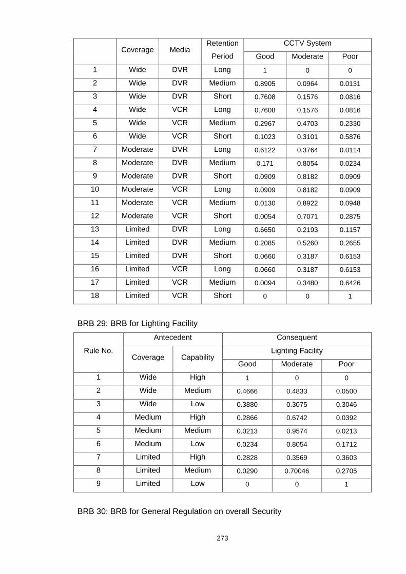
273
Coverage Media Retention
Period
CCTV System
Good Moderate Poor
1 Wide DVR Long 1 0 0
2 Wide DVR Medium 0.8905 0.0964 0.0131
3 Wide DVR Short 0.7608 0.1576 0.0816
4 Wide VCR Long 0.7608 0.1576 0.0816
5 Wide VCR Medium 0.2967 0.4703 0.2330
6 Wide VCR Short 0.1023 0.3101 0.5876
7 Moderate DVR Long 0.6122 0.3764 0.0114
8 Moderate DVR Medium 0.171 0.8054 0.0234
9 Moderate DVR Short 0.0909 0.8182 0.0909
10 Moderate VCR Long 0.0909 0.8182 0.0909
11 Moderate VCR Medium 0.0130 0.8922 0.0948
12 Moderate VCR Short 0.0054 0.7071 0.2875
13 Limited DVR Long 0.6650 0.2193 0.1157
14 Limited DVR Medium 0.2085 0.5260 0.2655
15 Limited DVR Short 0.0660 0.3187 0.6153
16 Limited VCR Long 0.0660 0.3187 0.6153
17 Limited VCR Medium 0.0094 0.3480 0.6426
18 Limited VCR Short 0 0 1
BRB 29: BRB for Lighting Facility
Rule No.
Antecedent Consequent
Coverage Capability Lighting Facility
Good Moderate Poor
1 Wide High 1 0 0
2 Wide Medium 0.4666 0.4833 0.0500
3 Wide Low 0.3880 0.3075 0.3046
4 Medium High 0.2866 0.6742 0.0392
5 Medium Medium 0.0213 0.9574 0.0213
6 Medium Low 0.0234 0.8054 0.1712
7 Limited High 0.2828 0.3569 0.3603
8 Limited Medium 0.0290 0.70046 0.2705
9 Limited Low 0 0 1
BRB 30: BRB for General Regulation on overall Security

274
Rule No.
Antecedent Consequent
RSC ISPS GR
Effective Moderate Not Effective
1 Effective Yes 1 0 0
2 Effective No 0.2240 0.3830 0.3930
3 Not Effective Yes 0.4912 0.5088 0
4 Not Effective No 0.0290 0.7005 0.2705
5 None Yes 0.4641 0.2714 0.2645
6 None No 0 0 1
RSC: Regulations for security culture, ISPS: Applic ation of ISPS Code, GR: General
Regulation on overall Security
BRB 31: BRB for Regulation on Access Control
Rule No.
Antecedent Consequent
TCE TTE TV Regulation on Access Control
Effective Moderate Not Effective
1 Yes Yes Yes 1 0 0
2 Yes Yes No 0.8125 0.1242 0.0633
3 Yes No Yes 0.7000 0.1965 0.1034
4 Yes No No 0.1350 0.3020 0.5630
5 No Yes Yes 0.5929 0.2650 0.1421
6 No Yes No 0.0883 0.3144 0.5973
7 No No Yes 0.0491 0.3210 0.6300
8 No No No 0 0 1
TCE: Towards Current Employees, TTE: Towards Termin ated Employees, TV: Towards
Visitors
BRB 32: BRB for Regulation on Procedure Control
Rule No.
Antecedent Consequent
PSL PSR Regulation on Procedure Control
Effective Moderate Not Effective
1 Yes Yes 1 0 0
2 Yes No 0.3333 0.3334 0.3333
3 No Yes 0.3333 0.3334 0.3333
4 No No 0 0 1
PSL: Procedure for stuffing and loading/unloading, Procedure for security incident report

275
BRB 33: BRB for Record
Rule No.
Antecedent Consequent
SR ER Record
Yes No
1 Yes Yes 1 0
2 Yes No 0.5 0.5
3 No Yes 0.5 0.5
4 No No 0 1
SR: Security system related records, ER: Employee r elated records
BRB 34: BRB for Cargo Inspection
Rule
No.
Antecedent Consequence
Inspection on
Containers
Inspection
on Trash
Cargo Inspection
Effective Moderate Not Effective
1 Good Yes 1 0 0
2 Good No 0.4183 0.3448 0.2368
3 Moderate Yes 0.2500 0.7124 0.0376
4 Moderate No 0.0277 0.7879 0.1843
5 Poor Yes 0.2513 0.3049 0.4438
6 Poor No 0 0 1
BRB 35: BRB for Security system related records
Rule No.
Antecedent Consequent
LAS LACS SR
Yes No
1 Yes Yes 1 0
2 Yes No 0.5 0.5
3 No Yes 0.5 0.5
4 No No 0 1
LAS: Logs of Alarm System, LACS: Logs of Access Con trol System, SR: Security system
related records
BRB 36: BRB for Employee related records
Rule No. Antecedent Consequent

276
REC RT RTE Employee related records
Yes No
1 Yes Yes Yes 1 0
2 Yes Yes No 0.6666 0.3334
3 Yes No Yes 0.6666 0.3334
4 Yes No No 0.3334 0.6666
5 No Yes Yes 0.6666 0.3334
6 No Yes No 0.3334 0.6666
7 No No Yes 0.3334 0.6666
8 No No No 0 1
REC: Records on Emergency Contact, RT: Records on T raining, RTE: Records on
terminated employees in recent 3 years
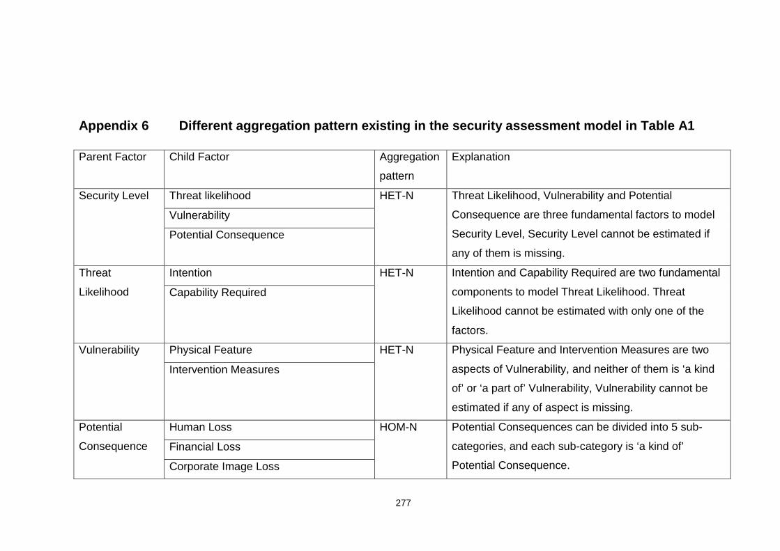
277
Appendix 6 Different aggregation pattern existing i n the security assessment model in Table A1
Parent Factor Child Factor Aggregation
pattern
Explanation
Security Level Threat likelihood HET-N Threat Likelihood, Vulnerability and Potential
Consequence are three fundamental factors to model
Security Level, Security Level cannot be estimated if
any of them is missing.
Vulnerability
Potential Consequence
Threat
Likelihood
Intention HET-N Intention and Capability Required are two fundamental
components to model Threat Likelihood. Threat
Likelihood cannot be estimated with only one of the
factors.
Capability Required
Vulnerability Physical Feature HET-N Physical Feature and Intervention Measures are two
aspects of Vulnerability, and neither of them is ‘a kind
of’ or ‘a part of’ Vulnerability, Vulnerability cannot be
estimated if any of aspect is missing.
Intervention Measures
Potential
Consequence
Human Loss HOM-N Potential Consequences can be divided into 5 sub-
categories, and each sub-category is ‘a kind of’
Potential Consequence.
Financial Loss
Corporate Image Loss

278
Economic Loss
Environment Loss
Capability
Required
Preventative Capability HET-N Preventative Capability and Cargo Magnitude are two
aspects of Capability Required, neither of them is ‘a
kind of’ or ‘a part of’ Capability Required, Capability
Required cannot be estimated if any of the aspect is
missing.
Cargo Magnitude
Physical
Feature
Historic Feature HOM-V Physical Feature has 3 sub-categories, and each
category is ‘a kind of’ physical feature. Among the 3
categories, if Historical Feature is not good, in general,
Facility Feature is more likely to be ‘Poor’ than to be
‘Good’. Thus, in general, the probability that Facility
Feature taking its referential values is influenced by the
referential values taken by Historic Feature. Therefore,
Historic Feature is a VIF of Facility Feature. Similarly,
Historic Feature is also a VIF of Employee Feature.
Employee Feature
Facility Feature
Intervention
Measures
Preventative Measures HOM-E There are 3 kinds of intervention activities: prevention,
response and recovery. The 3 parent factors are
corresponding to those 3 activities. In addition, as for
any security incident, prevention is more crucial than
Responsive Measures
Recovery Measures

279
response and recovery, if the utility of Preventative
Measures is under a threshold, the effect of
Responsive Measures and Recovery Measures on
Intervention Measures will be restricted. In other words,
low performance of Preventative Measures cannot be
compensated by high performance of either
Responsive Measures or Recovery Measures.
Therefore, Preventative Measures is an EIF of both
Responsive Measures and Recovery Measures
regarding Intervention Measures.
Facility Feature Hardware Feature HOM-E Both hardware and software are ‘a kind of’ facilities,
and Facility Feature has the same nature with both
Hardware Feature and Software Feature. In addition,
for a port, most of security related activities are
accomplished and supported by hardware, thus, if the
utility of Hardware Feature is below a certain threshold,
the effect of Software Feature on Facility Feature will
be influenced. In other words, low performance of
hardware cannot be compensated by high performance
of software. Therefore, Hardware Feature is an EIF of
Software Feature

280
Software Feature regarding Facility Feature
Preventative
Measures
Managerial Measures HOM-N Both Managerial Measures and Operative Measures
are ‘a kind of’ Preventative Measures. Operative Measures
Responsive
Measures
Response Activity HET-N Responsive Measures are modelled by both Response
Activity and Response Facility. Response Measures
cannot be estimated with only one element.
Response Facility
Hardware
Feature
Control Facility HOM-N The features of both Control Facility and Monitor
Facility are “a kind of” Hardware Feature. Monitor Facility
Managerial
Measures
Regulations HOM-E Development of Regulations and Management on
Regulations are two parts of Managerial Measures. If
the utility of Management on Regulations is below a
certain threshold, the impact of Regulations on
Managerial Measures will be limited. In other words,
low performance of Management on Regulations
cannot be compensated by high performance of
Regulations, therefore, Management on Regulation is
an EIF of Regulations regarding Managerial Measures.
Management on Regulations
Operative
Measures
Operations relevant to access control HOM-N All parent factors are ‘a kind of’ Operative Measures
and they share the same nature with Operative
Measures.
Operations relevant to employee
training/auditing
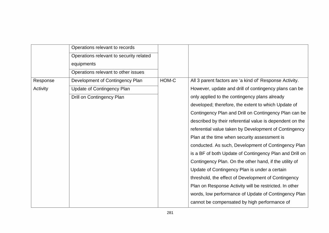
281
Operations relevant to records
Operations relevant to security related
equipments
Operations relevant to other issues
Response
Activity
Development of Contingency Plan HOM-C All 3 parent factors are ‘a kind of’ Response Activity.
However, update and drill of contingency plans can be
only applied to the contingency plans already
developed; therefore, the extent to which Update of
Contingency Plan and Drill on Contingency Plan can be
described by their referential value is dependent on the
referential value taken by Development of Contingency
Plan at the time when security assessment is
conducted. As such, Development of Contingency Plan
is a BF of both Update of Contingency Plan and Drill on
Contingency Plan. On the other hand, if the utility of
Update of Contingency Plan is under a certain
threshold, the effect of Development of Contingency
Plan on Response Activity will be restricted. In other
words, low performance of Update of Contingency Plan
cannot be compensated by high performance of
Update of Contingency Plan
Drill on Contingency Plan

282
Development of Contingency Plan. Therefore, Update
of Contingency Plan is an EIF of Development of
Contingency Plan regarding Response Activity.
Similarly, Drill of Contingency Plan is also an EIF of
Development of Contingency Plan regarding Response
Activity.
Response
Facility
Rescue Facility HOM-N Both Rescue Facility and Communication Facility are ‘a
kind of’ Response Facility. Communication Facility
Control Facility Access Control System HOM-N All the parent factors are ‘a part of’ Control Facility.
Alarm System
Connection between Access Control
System and Alarm System
Monitor Facility CCTV Facility HOM-E Both CCTV Facility and Lighting Facility are ‘a part of’
Monitor Facility. As CCTV Facility can function with its
full capacity only when lighting condition is not poor,
Lighting Facility is an EIF of CCTV Facility regarding
Monitor Facility, i.e., if the utility of Lighting Facility is
below a certain threshold, the effect of CCTV Facility
on Monitor Facility is limited, and thus low performance
of Lighting Facility cannot be compensated by high
Lighting Facility

283
performance of CCTV Facility.
Regulations General Regulations regarding overall
security
HOM-N All parent factors are ‘a part of’ regulations
Regulations regarding access control
Regulations regarding procedure control
Management on
Regulations
Monitor on execution status of
regulations
HOM-N Monitor, Audit and Update are all ‘a kind of’
Management on Regulations.
Audit on execution status of regulations
Update on regulations
Operations
relevant to
access control
Photo-ID Badge HOM-N Both parent factors can be considered as ‘a kind of’
Operations relevant to access control Key/Key Card
Operations
relevant to
employee
training/auditing
Training of employee HOM-N Both parent factors are ‘a kind of’ Operations relevant
to employee training/auditing. Auditing of current status of employee
Operations
relevant to
records
Keeping of Records HOM-C All the parent factors are ‘a kind of’ Operations relevant
to Records. As protection and management of records
can be only applied to existing records, the extent to
which Protection of Records and Management of
Protection of Records
Management of Records

284
Records can be described by their referential value is
influenced by referential value taken by Keeping of
Records. Therefore, Keeping of Records is a BF to
both Protection of Records and Management of
Records. On the other hand, as poor protection of
records may lead to unauthorized access to the
records, when the utility of Protection of Records is
below a certain threshold, the effects of Keeping of
Records and Management of Records on Operations
relevant to records are influenced, in other words, low
performance of Protection of Records cannot be
compensated by high performance of Keeping of
Records or Management of Records. Therefore,
Protection of Records is an EIF of Keeping of Records
and Management of Records regarding Operations
relevant to records. Similarly, Management of Records
is an EIF of Keeping of Records and Protection of
Records regarding Operations relevant to records.
Operations
relevant to
Control on cargo-handling equipments HOM-N All parent factors are ‘a kind of’ Operations relevant to
security related equipments. Test/maintenance/repair for security

285
security related
equipments
systems
UPS equipments or other forms of
emergency power supply of security
systems
Operations
relevant to other
issues
Operations relevant to cargo inspection HOM-N All parent factors are ‘a kind of’ Operations relevant to
other issues Operations relevant to vulnerability
assessment
Operations relevant to guarding and
patrolling
Rescue facility Capability HET-N Capability and Availability are 2 essential factors to
model Rescue Facility. The nature of the 3 factors is
different from each other.
Availability
Access Control
System
Coverage HET-N Access Control System is modelled by the 3
components represented by 3 parent factors. The
performance of Access Control System cannot be
estimated if any of the 3 components is missing.
Capability
Robustness
Alarm System Capability HET-N Capability and Robustness are two essential attributes
to describe Alarm System, neither of them has the
same nature as Alarm System.
Robustness
CCTV Facility Coverage HET-N All parent factors are the attributes used to describe
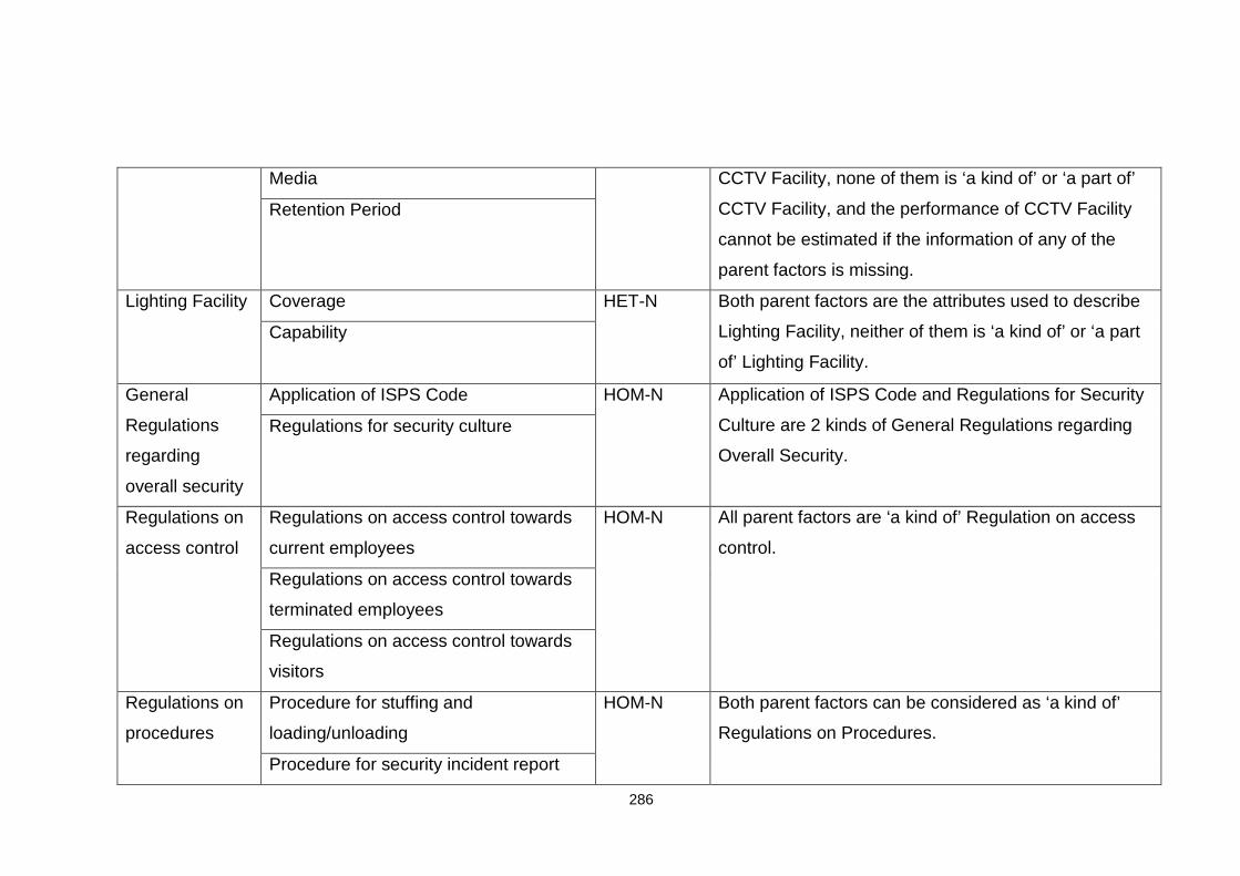
286
Media CCTV Facility, none of them is ‘a kind of’ or ‘a part of’
CCTV Facility, and the performance of CCTV Facility
cannot be estimated if the information of any of the
parent factors is missing.
Retention Period
Lighting Facility Coverage HET-N Both parent factors are the attributes used to describe
Lighting Facility, neither of them is ‘a kind of’ or ‘a part
of’ Lighting Facility.
Capability
General
Regulations
regarding
overall security
Application of ISPS Code HOM-N Application of ISPS Code and Regulations for Security
Culture are 2 kinds of General Regulations regarding
Overall Security.
Regulations for security culture
Regulations on
access control
Regulations on access control towards
current employees
HOM-N All parent factors are ‘a kind of’ Regulation on access
control.
Regulations on access control towards
terminated employees
Regulations on access control towards
visitors
Regulations on
procedures
Procedure for stuffing and
loading/unloading
HOM-N Both parent factors can be considered as ‘a kind of’
Regulations on Procedures.
Procedure for security incident report
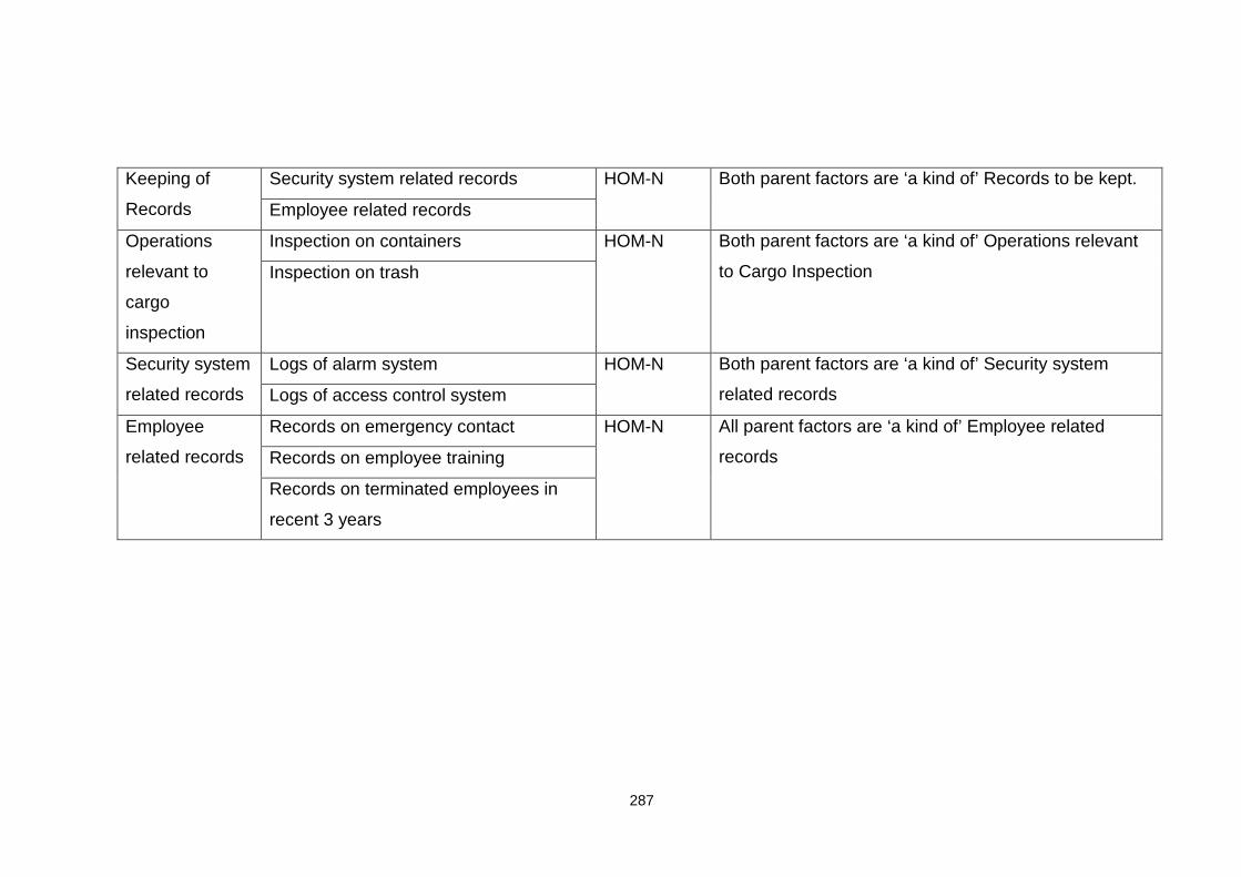
287
Keeping of
Records
Security system related records HOM-N Both parent factors are ‘a kind of’ Records to be kept.
Employee related records
Operations
relevant to
cargo
inspection
Inspection on containers HOM-N Both parent factors are ‘a kind of’ Operations relevant
to Cargo Inspection Inspection on trash
Security system
related records
Logs of alarm system HOM-N Both parent factors are ‘a kind of’ Security system
related records Logs of access control system
Employee
related records
Records on emergency contact HOM-N All parent factors are ‘a kind of’ Employee related
records Records on employee training
Records on terminated employees in
recent 3 years

288
Appendix 7 Belief Rule Bases for the security asses sment model in Appendix 1 with a homogeneous information aggregation pattern
BRB 4: BRB for Potential Consequence
Rule
No.
Antecedent Consequence
HL FL CIL EL ENL Potential Consequence
CA S M NS N
1 H H Y H Y 1 0 0 0 0
2 H H Y H N 1 0 0 0 0
3 H H Y L Y 1 0 0 0 0
4 H H Y L N 1 0 0 0 0
5 H H Y N Y 1 0 0 0 0
6 H H Y N N 1 0 0 0 0
7 H H N H Y 1 0 0 0 0
8 H H N H N 1 0 0 0 0
9 H H N L Y 1 0 0 0 0
10 H H N L N 1 0 0 0 0
11 H H N N Y 1 0 0 0 0
12 H H N N N 1 0 0 0 0
13 H L Y H Y 1 0 0 0 0
14 H L Y H N 1 0 0 0 0
15 H L Y L Y 1 0 0 0 0
16 H L Y L N 1 0 0 0 0
17 H L Y N Y 1 0 0 0 0
18 H L Y N N 1 0 0 0 0
19 H L N H Y 1 0 0 0 0
20 H L N H N 1 0 0 0 0
21 H L N L Y 1 0 0 0 0
22 H L N L N 1 0 0 0 0
23 H L N N Y 1 0 0 0 0
24 H L N N N 1 0 0 0 0
25 H N Y H Y 1 0 0 0 0
26 H N Y H N 1 0 0 0 0
27 H N Y L Y 1 0 0 0 0

289
28 H N Y L N 1 0 0 0 0
29 H N Y N Y 1 0 0 0 0
30 H N Y N N 1 0 0 0 0
31 H N N H Y 1 0 0 0 0
32 H N N H N 1 0 0 0 0
33 H N N L Y 1 0 0 0 0
34 H N N L N 1 0 0 0 0
35 H N N N Y 1 0 0 0 0
36 H N N N N 1 0 0 0 0
37 L H Y H Y 0.2843 0.2533 0.1862 0.1994 0.0769
38 L H Y H N 0.2920 0.2513 0.1769 0.0954 0.1844
39 L H Y L Y 0.2640 0.1522 0.1829 0.3028 0.0981
40 L H Y L N 0.2717 0.1502 0.1736 0.1988 0.2056
41 L H Y N Y 0.2717 0.1502 0.1736 0.1988 0.2056
42 L H Y N N 0.2794 0.1483 0.1644 0.0948 0.3130
43 L H N H Y 0.2685 0.2346 0.1179 0.1808 0.1982
44 L H N H N 0.2762 0.2327 0.1086 0.0768 0.3057
45 L H N L Y 0.2483 0.1335 0.1146 0.2842 0.2194
46 L H N L N 0.2560 0.1316 0.1053 0.1802 0.3268
47 L H N N Y 0.2560 0.1316 0.1053 0.1802 0.3268
48 L H N N N 0.2637 0.1297 0.0961 0.0762 0.4343
49 L L Y H Y 0.2066 0.2455 0.2449 0.2184 0.0846
50 L L Y H N 0.2143 0.2436 0.2356 0.1144 0.1921
51 L L Y L Y 0.1864 0.1444 0.2416 0.3218 0.1058
52 L L Y L N 0.1941 0.1425 0.2324 0.2178 0.2133
53 L L Y N Y 0.1941 0.1425 0.2324 0.2178 0.2133
54 L L Y N N 0.2018 0.1405 0.2231 0.1138 0.3208
55 L L N H Y 0.1909 0.2269 0.1766 0.1997 0.2059
56 L L N H N 0.1986 0.2250 0.1673 0.0957 0.3134
57 L L N L Y 0.1707 0.1258 0.1733 0.3032 0.2271
58 L L N L N 0.1784 0.1238 0.1641 0.1992 0.3346
59 L L N N Y 0.1784 0.1238 0.1641 0.1992 0.3346
60 L L N N N 0.1861 0.1219 0.1548 0.0952 0.4420
61 L N Y H Y 0.1909 0.2269 0.1766 0.1997 0.2059
62 L N Y H N 0.1986 0.2250 0.1673 0.0957 0.3134

290
63 L N Y L Y 0.1707 0.1258 0.1733 0.3032 0.2271
64 L N Y L N 0.1784 0.1238 0.1641 0.1992 0.3346
65 L N Y N Y 0.1784 0.1238 0.1641 0.1992 0.3346
66 L N Y N N 0.1861 0.1219 0.1548 0.0952 0.4420
67 L N N H Y 0.1751 0.2083 0.1083 0.1811 0.3272
68 L N N H N 0.1828 0.2063 0.0990 0.0771 0.4347
69 L N N L Y 0.1549 0.1071 0.1050 0.2846 0.3484
70 L N N L N 0.1626 0.1052 0.0958 0.1806 0.4558
71 L N N N Y 0.1626 0.1052 0.0958 0.1806 0.4558
72 L N N N N 0.1703 0.1033 0.0865 0.0766 0.5633
73 N H Y H Y 0.1909 0.2269 0.1766 0.1997 0.2059
74 N H Y H N 0.1986 0.2250 0.1673 0.0957 0.3134
75 N H Y L Y 0.1707 0.1258 0.1733 0.3032 0.2271
76 N H Y L N 0.1784 0.1238 0.1641 0.1992 0.3346
77 N H Y N Y 0.1784 0.1238 0.1641 0.1992 0.3346
78 N H Y N N 0.1861 0.1219 0.1548 0.0952 0.4420
79 N H N H Y 0.1751 0.2083 0.1083 0.1811 0.3272
80 N H N H N 0.1828 0.2063 0.0990 0.0771 0.4347
81 N H N L Y 0.1549 0.1071 0.1050 0.2846 0.3484
82 N H N L N 0.1626 0.1052 0.0958 0.1806 0.4558
83 N H N N Y 0.1626 0.1052 0.0958 0.1806 0.4558
84 N H N N N 0.1703 0.1033 0.0865 0.0766 0.5633
85 N L Y H Y 0.1132 0.2191 0.2353 0.2187 0.2136
86 N L Y H N 0.1209 0.2172 0.2260 0.1147 0.3211
87 N L Y L Y 0.0930 0.1180 0.2320 0.3222 0.2348
88 N L Y L N 0.1007 0.1161 0.2228 0.2182 0.3423
89 N L Y N Y 0.1007 0.1161 0.2228 0.2182 0.3423
90 N L Y N N 0.1084 0.1142 0.2135 0.1142 0.4497
91 N L N H Y 0.0975 0.2005 0.1670 0.2001 0.3349
92 N L N H N 0.1052 0.1986 0.1577 0.0961 0.4424
93 N L N L Y 0.0773 0.0994 0.1638 0.3035 0.3561
94 N L N L N 0.0850 0.0975 0.1545 0.1995 0.4635
95 N L N N Y 0.0850 0.0975 0.1545 0.1995 0.4635
96 N L N N N 0.0927 0.0955 0.1452 0.0955 0.5710
97 N N Y H Y 0.0975 0.2005 0.1670 0.2001 0.3349

291
98 N N Y H N 0.1052 0.1986 0.1577 0.0961 0.4424
99 N N Y L Y 0.0773 0.0994 0.1638 0.3035 0.3561
100 N N Y L N 0.0850 0.0975 0.1545 0.1995 0.4635
101 N N Y N Y 0.0850 0.0975 0.1545 0.1995 0.4635
102 N N Y N N 0.0927 0.0955 0.1452 0.0955 0.5710
103 N N N H Y 0.0818 0.1819 0.0987 0.1815 0.4562
104 N N N H N 0.0895 0.1800 0.0895 0.0775 0.5637
105 N N N L Y 0.0615 0.0808 0.0955 0.2849 0.4773
106 N N N L N 0.0692 0.0788 0.0862 0.1809 0.5848
107 N N N N Y 0.0692 0.0788 0.0862 0.1809 0.5848
108 N N N N N 0 0 0 0 1
HL: Human Loss, FL: Financial Loss, CIL: Cooperate Image Loss, EL: Economic Loss,
ENL: Environmental Loss
H: High, L: Low, N: None, Y: Yes, N: No, CAT: Catas trophic, S: Severe, M: Moderate, NS:
Not Severe, N: None
BRB 6: BRB for Physical Feature
Rule No.
Antecedent Consequence
Historic
Features
Employee
Features
Facility
Features
Physical Feature
Good Moderate Poor
1 Good Good Good 1 0 0
2 Good Good Moderate 0.5556 0.3161 0.1282
3 Good Good Poor 0.5135 0.1567 0.3297
4 Good Poor Good 0.5194 0.2216 0.2590
5 Good Poor Moderate 0.3325 0.3691 0.2984
6 Good Poor Poor 0.2904 0.2097 0.4999
7 Moderate Good Good 0.5835 0.2747 0.1418
8 Moderate Good Moderate 0.3965 0.4222 0.1813
9 Moderate Good Poor 0.3545 0.2628 0.3827
10 Moderate Poor Good 0.3603 0.3277 0.3120
11 Moderate Poor Moderate 0.1734 0.4752 0.3515
12 Moderate Poor Poor 0.1313 0.3158 0.5529
13 Poor Good Good 0.5235 0.2166 0.2599
14 Poor Good Moderate 0.3366 0.3640 0.2994
15 Poor Good Poor 0.2945 0.2046 0.5009
16 Poor Poor Good 0.3003 0.2695 0.4301

292
17 Poor Poor Moderate 0.1134 0.4170 0.4696
18 Poor Poor Poor 0 0 1
BRB 7: BRB for Intervention Measures
Rule
No.
Antecedent Consequence
PM RCM RSM Intervention Measures
Effective Moderate Not Effective
1 Effective Effective Effective 1 0 0
2 Effective Effective Moderate 0.5835 0.2747 0.1418
3 Effective Effective Not Effective 0.5235 0.2166 0.2599
4 Effective Not Effective Effective 0.5273 0.2150 0.2577
5 Effective Not Effective Moderate 0.3603 0.3277 0.3120
6 Effective Not Effective Not Effective 0.3003 0.2695 0.4301
7 Moderate Effective Effective 0.5802 0.2761 0.1437
8 Moderate Effective Moderate 0.4132 0.3889 0.1979
9 Moderate Effective Not Effective 0.3532 0.3307 0.3161
10 Moderate Not Effective Effective 0.3571 0.3291 0.3138
11 Moderate Not Effective Moderate 0.1900 0.4418 0.3681
12 Moderate Not Effective Not Effective 0.1301 0.3837 0.4862
13 Not Effective Effective Effective 0.5189 0.2157 0.2654
14 Not Effective Effective Moderate 0.3519 0.3284 0.3197
15 Not Effective Effective Not Effective 0.2919 0.2703 0.4378
16 Not Effective Not Effective Effective 0.2957 0.2687 0.4356
17 Not Effective Not Effective Moderate 0.1287 0.3814 0.4899
18 Not Effective Not Effective Not Effective 0 0 1
PM: Preventative Measures, RCM: Recovery Measures, RSM: Response Measures
BRB 8: BRB for Facility Feature
Rule No.
Antecedent Consequence
Hardware
Feature
Software
Feature
Facility Feature
Good Moderate Poor
1 Good Good 1 0 0
2 Good Poor 0.4177 0.2431 0.3393
3 Moderate Good 0.3863 0.5170 0.0967
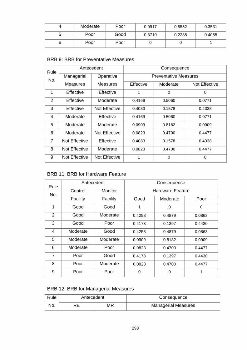
293
4 Moderate Poor 0.0917 0.5552 0.3531
5 Poor Good 0.3710 0.2235 0.4055
6 Poor Poor 0 0 1
BRB 9: BRB for Preventative Measures
Rule
No.
Antecedent Consequence
Managerial
Measures
Operative
Measures
Preventative Measures
Effective Moderate Not Effective
1 Effective Effective 1 0 0
2 Effective Moderate 0.4169 0.5060 0.0771
3 Effective Not Effective 0.4083 0.1578 0.4338
4 Moderate Effective 0.4169 0.5060 0.0771
5 Moderate Moderate 0.0909 0.8182 0.0909
6 Moderate Not Effective 0.0823 0.4700 0.4477
7 Not Effective Effective 0.4083 0.1578 0.4338
8 Not Effective Moderate 0.0823 0.4700 0.4477
9 Not Effective Not Effective 1 0 0
BRB 11: BRB for Hardware Feature
Rule
No.
Antecedent Consequence
Control
Facility
Monitor
Facility
Hardware Feature
Good Moderate Poor
1 Good Good 1 0 0
2 Good Moderate 0.4258 0.4879 0.0863
3 Good Poor 0.4173 0.1397 0.4430
4 Moderate Good 0.4258 0.4879 0.0863
5 Moderate Moderate 0.0909 0.8182 0.0909
6 Moderate Poor 0.0823 0.4700 0.4477
7 Poor Good 0.4173 0.1397 0.4430
8 Poor Moderate 0.0823 0.4700 0.4477
9 Poor Poor 0 0 1
BRB 12: BRB for Managerial Measures
Rule
No.
Antecedent Consequence
RE MR Managerial Measures
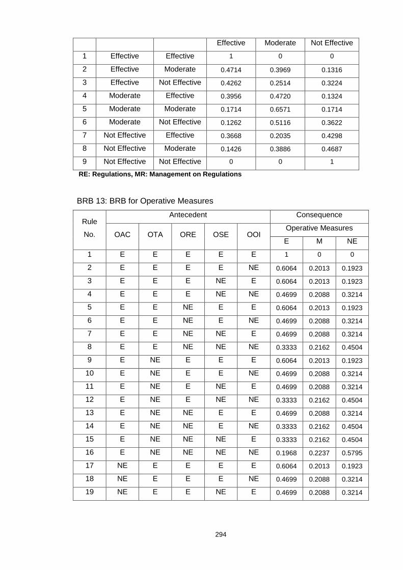
294
Effective Moderate Not Effective
1 Effective Effective 1 0 0
2 Effective Moderate 0.4714 0.3969 0.1316
3 Effective Not Effective 0.4262 0.2514 0.3224
4 Moderate Effective 0.3956 0.4720 0.1324
5 Moderate Moderate 0.1714 0.6571 0.1714
6 Moderate Not Effective 0.1262 0.5116 0.3622
7 Not Effective Effective 0.3668 0.2035 0.4298
8 Not Effective Moderate 0.1426 0.3886 0.4687
9 Not Effective Not Effective 0 0 1
RE: Regulations, MR: Management on Regulations
BRB 13: BRB for Operative Measures
Rule
No.
Antecedent Consequence
OAC OTA ORE OSE OOI Operative Measures
E M NE
1 E E E E E 1 0 0
2 E E E E NE 0.6064 0.2013 0.1923
3 E E E NE E 0.6064 0.2013 0.1923
4 E E E NE NE 0.4699 0.2088 0.3214
5 E E NE E E 0.6064 0.2013 0.1923
6 E E NE E NE 0.4699 0.2088 0.3214
7 E E NE NE E 0.4699 0.2088 0.3214
8 E E NE NE NE 0.3333 0.2162 0.4504
9 E NE E E E 0.6064 0.2013 0.1923
10 E NE E E NE 0.4699 0.2088 0.3214
11 E NE E NE E 0.4699 0.2088 0.3214
12 E NE E NE NE 0.3333 0.2162 0.4504
13 E NE NE E E 0.4699 0.2088 0.3214
14 E NE NE E NE 0.3333 0.2162 0.4504
15 E NE NE NE E 0.3333 0.2162 0.4504
16 E NE NE NE NE 0.1968 0.2237 0.5795
17 NE E E E E 0.6064 0.2013 0.1923
18 NE E E E NE 0.4699 0.2088 0.3214
19 NE E E NE E 0.4699 0.2088 0.3214
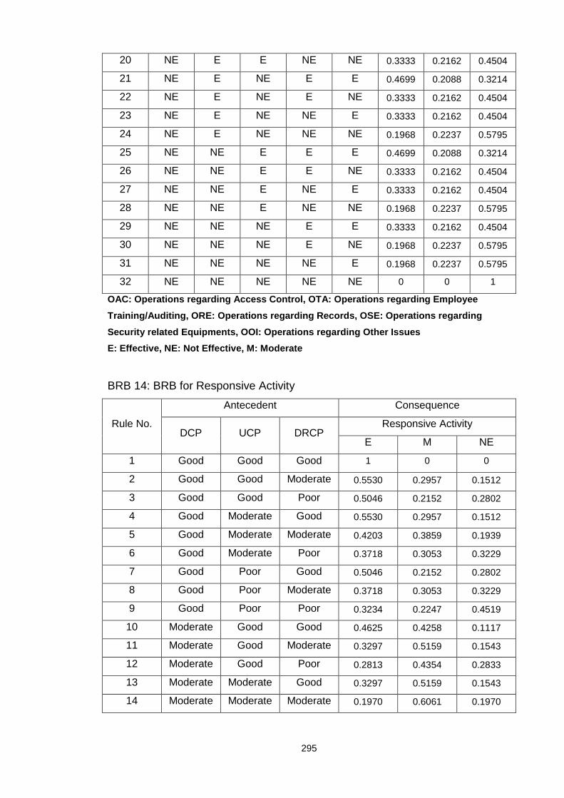
295
20 NE E E NE NE 0.3333 0.2162 0.4504
21 NE E NE E E 0.4699 0.2088 0.3214
22 NE E NE E NE 0.3333 0.2162 0.4504
23 NE E NE NE E 0.3333 0.2162 0.4504
24 NE E NE NE NE 0.1968 0.2237 0.5795
25 NE NE E E E 0.4699 0.2088 0.3214
26 NE NE E E NE 0.3333 0.2162 0.4504
27 NE NE E NE E 0.3333 0.2162 0.4504
28 NE NE E NE NE 0.1968 0.2237 0.5795
29 NE NE NE E E 0.3333 0.2162 0.4504
30 NE NE NE E NE 0.1968 0.2237 0.5795
31 NE NE NE NE E 0.1968 0.2237 0.5795
32 NE NE NE NE NE 0 0 1
OAC: Operations regarding Access Control, OTA: Oper ations regarding Employee
Training/Auditing, ORE: Operations regarding Record s, OSE: Operations regarding
Security related Equipments, OOI: Operations regard ing Other Issues
E: Effective, NE: Not Effective, M: Moderate
BRB 14: BRB for Responsive Activity
Rule No.
Antecedent Consequence
DCP UCP DRCP Responsive Activity
E M NE
1 Good Good Good 1 0 0
2 Good Good Moderate 0.5530 0.2957 0.1512
3 Good Good Poor 0.5046 0.2152 0.2802
4 Good Moderate Good 0.5530 0.2957 0.1512
5 Good Moderate Moderate 0.4203 0.3859 0.1939
6 Good Moderate Poor 0.3718 0.3053 0.3229
7 Good Poor Good 0.5046 0.2152 0.2802
8 Good Poor Moderate 0.3718 0.3053 0.3229
9 Good Poor Poor 0.3234 0.2247 0.4519
10 Moderate Good Good 0.4625 0.4258 0.1117
11 Moderate Good Moderate 0.3297 0.5159 0.1543
12 Moderate Good Poor 0.2813 0.4354 0.2833
13 Moderate Moderate Good 0.3297 0.5159 0.1543
14 Moderate Moderate Moderate 0.1970 0.6061 0.1970
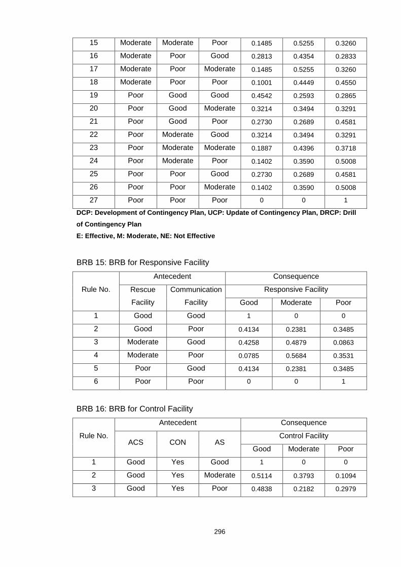
296
15 Moderate Moderate Poor 0.1485 0.5255 0.3260
16 Moderate Poor Good 0.2813 0.4354 0.2833
17 Moderate Poor Moderate 0.1485 0.5255 0.3260
18 Moderate Poor Poor 0.1001 0.4449 0.4550
19 Poor Good Good 0.4542 0.2593 0.2865
20 Poor Good Moderate 0.3214 0.3494 0.3291
21 Poor Good Poor 0.2730 0.2689 0.4581
22 Poor Moderate Good 0.3214 0.3494 0.3291
23 Poor Moderate Moderate 0.1887 0.4396 0.3718
24 Poor Moderate Poor 0.1402 0.3590 0.5008
25 Poor Poor Good 0.2730 0.2689 0.4581
26 Poor Poor Moderate 0.1402 0.3590 0.5008
27 Poor Poor Poor 0 0 1
DCP: Development of Contingency Plan, UCP: Update o f Contingency Plan, DRCP: Drill
of Contingency Plan
E: Effective, M: Moderate, NE: Not Effective
BRB 15: BRB for Responsive Facility
Rule No.
Antecedent Consequence
Rescue
Facility
Communication
Facility
Responsive Facility
Good Moderate Poor
1 Good Good 1 0 0
2 Good Poor 0.4134 0.2381 0.3485
3 Moderate Good 0.4258 0.4879 0.0863
4 Moderate Poor 0.0785 0.5684 0.3531
5 Poor Good 0.4134 0.2381 0.3485
6 Poor Poor 0 0 1
BRB 16: BRB for Control Facility
Rule No.
Antecedent Consequence
ACS CON AS Control Facility
Good Moderate Poor
1 Good Yes Good 1 0 0
2 Good Yes Moderate 0.5114 0.3793 0.1094
3 Good Yes Poor 0.4838 0.2182 0.2979

297
4 Good No Good 0.5317 0.2323 0.2360
5 Good No Moderate 0.3317 0.4057 0.2626
6 Good No Poor 0.3042 0.2447 0.4511
7 Moderate Yes Good 0.5114 0.3793 0.1094
8 Moderate Yes Moderate 0.3113 0.5527 0.1359
9 Moderate Yes Poor 0.2838 0.3917 0.3245
10 Moderate No Good 0.3317 0.4057 0.2626
11 Moderate No Moderate 0.1317 0.5792 0.2891
12 Moderate No Poor 0.1042 0.4181 0.4776
13 Poor Yes Good 0.4838 0.2182 0.2979
14 Poor Yes Moderate 0.2838 0.3917 0.3245
15 Poor Yes Poor 0.2563 0.2306 0.5130
16 Poor No Good 0.3042 0.2447 0.4511
17 Poor No Moderate 0.1042 0.4181 0.4776
18 Poor No Poor 0 0 1
ACS: Access Control System, AS: Alarm System, CON: Connection between ACS and AS
BRB 17: BRB for Monitor Facility
Rule No.
Antecedent Consequence
CCTV
Facility
Lighting
Facility
Monitor Facility
Good Moderate Poor
1 Good Good 1 0 0
2 Good Moderate 0.4258 0.4879 0.0863
3 Good Poor 0.4173 0.1397 0.4430
4 Moderate Good 0.4258 0.4879 0.0863
5 Moderate Moderate 0.0909 0.8182 0.0909
6 Moderate Poor 0.0823 0.4700 0.4477
7 Poor Good 0.4173 0.1397 0.4430
8 Poor Moderate 0.0823 0.4700 0.4477
9 Poor Poor 0 0 1
BRB 18: BRB for Regulations
Rule
No.
Antecedent Consequence
GR RAC RPC Regulations
E M NE

298
1 Effective Effective Effective 1 0 0
2 Effective Effective Moderate 0.5872 0.4128 0.0000
3 Effective Effective Not Effective 0.5292 0.2113 0.2595
4 Effective Moderate Effective 0.5872 0.4128 0.0000
5 Effective Moderate Moderate 0.3444 0.6556 0.0000
6 Effective Moderate Not Effective 0.3059 0.4315 0.2626
7 Effective Not Effective Effective 0.5292 0.2113 0.2595
8 Effective Not Effective Moderate 0.3059 0.4315 0.2626
9 Effective Not Effective Not Effective 0.2976 0.2650 0.4374
10 Moderate Effective Effective 0.5872 0.4128 0.0000
11 Moderate Effective Moderate 0.3444 0.6556 0.0000
12 Moderate Effective Not Effective 0.3059 0.4315 0.2626
13 Moderate Moderate Effective 0.3444 0.6556 0.0000
14 Moderate Moderate Moderate 0.1000 0.9000 0.0000
15 Moderate Moderate Not Effective 0.0826 0.6517 0.2657
16 Moderate Not Effective Effective 0.3059 0.4315 0.2626
17 Moderate Not Effective Moderate 0.0826 0.6517 0.2657
18 Moderate Not Effective Not Effective 0.0743 0.4852 0.4405
19 Not Effective Effective Effective 0.5292 0.2113 0.2595
20 Not Effective Effective Moderate 0.3059 0.4315 0.2626
21 Not Effective Effective Not Effective 0.2976 0.2650 0.4374
22 Not Effective Moderate Effective 0.3059 0.4315 0.2626
23 Not Effective Moderate Moderate 0.0826 0.6517 0.2657
24 Not Effective Moderate Not Effective 0.0743 0.4852 0.4405
25 Not Effective Not Effective Effective 0.2976 0.2650 0.4374
26 Not Effective Not Effective Moderate 0.0743 0.4852 0.4405
27 Not Effective Not Effective Not Effective 0 0 1
GR: General Regulation on overall Security, RAC: Re gulation on Access Control, RPC:
Regulation on Process Control
BRB 19: BRB for Management on Regulations
Rule No.
Antecedent Consequence
ME AE UR Management on Regulations
E M NE
1 Yes Yes Yes 1 0 0
2 Yes Yes No 0.5292 0.2113 0.2595
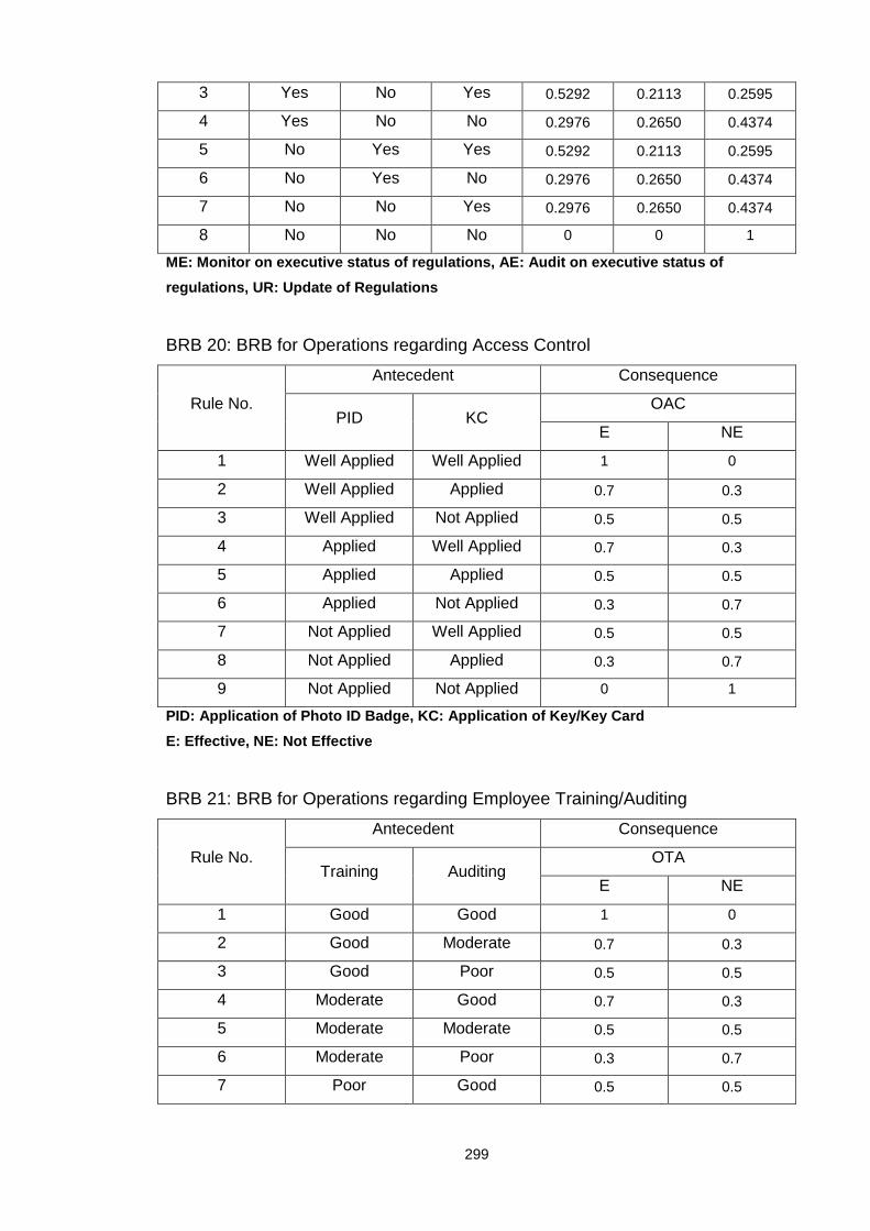
299
3 Yes No Yes 0.5292 0.2113 0.2595
4 Yes No No 0.2976 0.2650 0.4374
5 No Yes Yes 0.5292 0.2113 0.2595
6 No Yes No 0.2976 0.2650 0.4374
7 No No Yes 0.2976 0.2650 0.4374
8 No No No 0 0 1
ME: Monitor on executive status of regulations, AE: Audit on executive status of
regulations, UR: Update of Regulations
BRB 20: BRB for Operations regarding Access Control
Rule No.
Antecedent Consequence
PID KC OAC
E NE
1 Well Applied Well Applied 1 0
2 Well Applied Applied 0.7 0.3
3 Well Applied Not Applied 0.5 0.5
4 Applied Well Applied 0.7 0.3
5 Applied Applied 0.5 0.5
6 Applied Not Applied 0.3 0.7
7 Not Applied Well Applied 0.5 0.5
8 Not Applied Applied 0.3 0.7
9 Not Applied Not Applied 0 1
PID: Application of Photo ID Badge, KC: Application of Key/Key Card
E: Effective, NE: Not Effective
BRB 21: BRB for Operations regarding Employee Training/Auditing
Rule No.
Antecedent Consequence
Training Auditing OTA
E NE
1 Good Good 1 0
2 Good Moderate 0.7 0.3
3 Good Poor 0.5 0.5
4 Moderate Good 0.7 0.3
5 Moderate Moderate 0.5 0.5
6 Moderate Poor 0.3 0.7
7 Poor Good 0.5 0.5
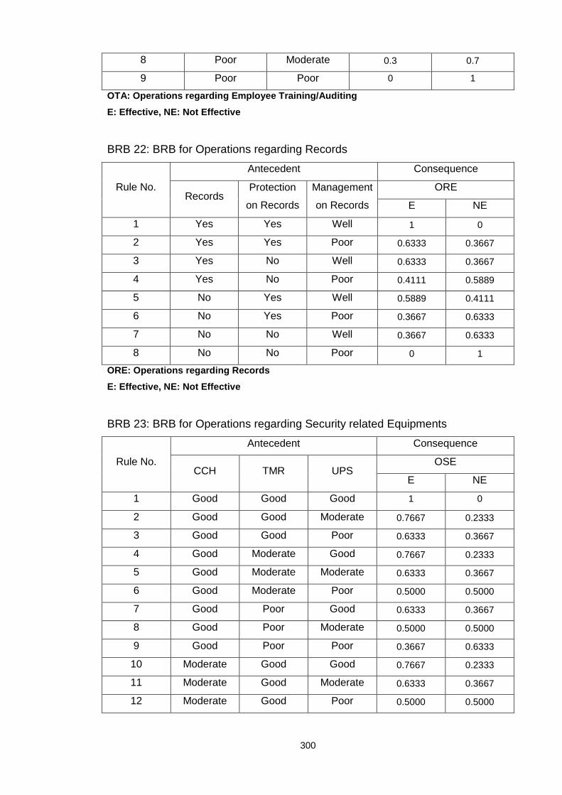
300
8 Poor Moderate 0.3 0.7
9 Poor Poor 0 1
OTA: Operations regarding Employee Training/Auditin g
E: Effective, NE: Not Effective
BRB 22: BRB for Operations regarding Records
Rule No.
Antecedent Consequence
Records Protection
on Records
Management
on Records
ORE
E NE
1 Yes Yes Well 1 0
2 Yes Yes Poor 0.6333 0.3667
3 Yes No Well 0.6333 0.3667
4 Yes No Poor 0.4111 0.5889
5 No Yes Well 0.5889 0.4111
6 No Yes Poor 0.3667 0.6333
7 No No Well 0.3667 0.6333
8 No No Poor 0 1
ORE: Operations regarding Records
E: Effective, NE: Not Effective
BRB 23: BRB for Operations regarding Security related Equipments
Rule No.
Antecedent Consequence
CCH TMR UPS OSE
E NE
1 Good Good Good 1 0
2 Good Good Moderate 0.7667 0.2333
3 Good Good Poor 0.6333 0.3667
4 Good Moderate Good 0.7667 0.2333
5 Good Moderate Moderate 0.6333 0.3667
6 Good Moderate Poor 0.5000 0.5000
7 Good Poor Good 0.6333 0.3667
8 Good Poor Moderate 0.5000 0.5000
9 Good Poor Poor 0.3667 0.6333
10 Moderate Good Good 0.7667 0.2333
11 Moderate Good Moderate 0.6333 0.3667
12 Moderate Good Poor 0.5000 0.5000

301
13 Moderate Moderate Good 0.6333 0.3667
14 Moderate Moderate Moderate 0.5000 0.5000
15 Moderate Moderate Poor 0.3667 0.6333
16 Moderate Poor Good 0.5000 0.5000
17 Moderate Poor Moderate 0.3667 0.6333
18 Moderate Poor Poor 0.2333 0.7667
19 Poor Good Good 0.6333 0.3667
20 Poor Good Moderate 0.5000 0.5000
21 Poor Good Poor 0.3667 0.6333
22 Poor Moderate Good 0.5000 0.5000
23 Poor Moderate Moderate 0.3667 0.6333
24 Poor Moderate Poor 0.2333 0.7667
25 Poor Poor Good 0.3667 0.6333
26 Poor Poor Moderate 0.2333 0.7667
27 Poor Poor Poor 0 1
CCH: Control on cargo-handling equipments, TMR: Tes t/maintenance/repair for security
systems, UPS: UPS equipments on security systems, O SE: Operations regarding
Security related Equipments
E: Effective, NE: Not Effective
BRB 24: BRB for Operations regarding Other Issues
Rule No.
Antecedent Consequence
CI VA GP OOI
E NE
1 Effective Frequent Enough 1 0
2 Effective Frequent Not Enough 0.6333 0.3667
3 Effective Standard Enough 0.7667 0.2333
4 Effective Standard Not Enough 0.5000 0.5000
5 Effective None Enough 0.6333 0.3667
6 Effective None Not Enough 0.3667 0.6333
7 Moderate Frequent Enough 0.7667 0.2333
8 Moderate Frequent Not Enough 0.5000 0.5000
9 Moderate Standard Enough 0.6333 0.3667
10 Moderate Standard Not Enough 0.3667 0.6333
11 Moderate None Enough 0.5000 0.5000
12 Moderate None Not Enough 0.2333 0.7667
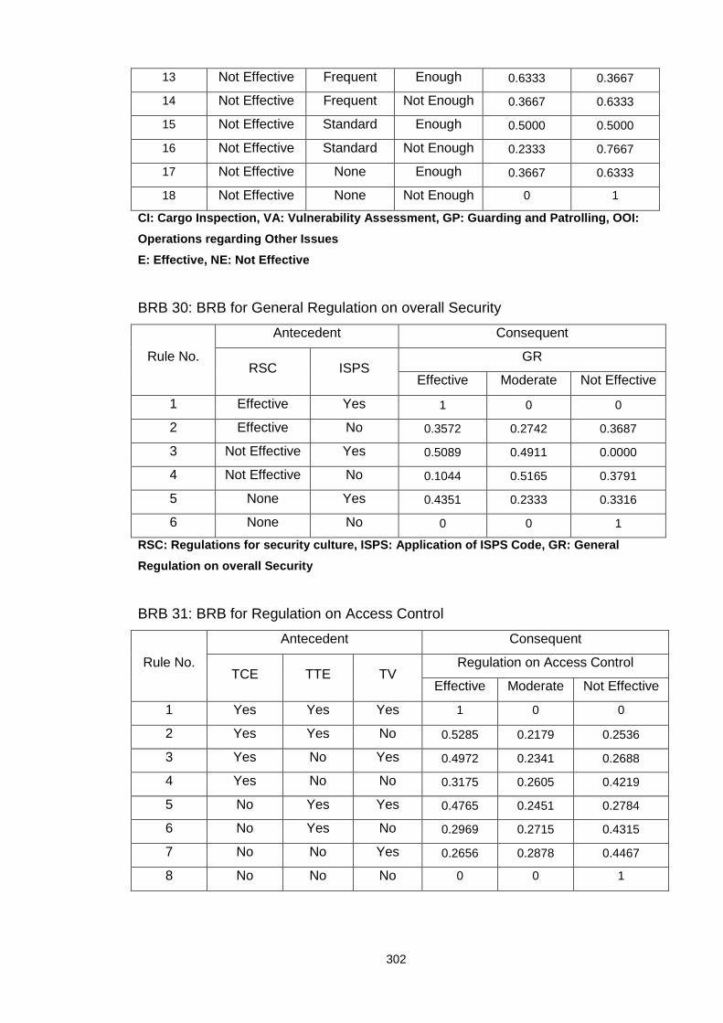
302
13 Not Effective Frequent Enough 0.6333 0.3667
14 Not Effective Frequent Not Enough 0.3667 0.6333
15 Not Effective Standard Enough 0.5000 0.5000
16 Not Effective Standard Not Enough 0.2333 0.7667
17 Not Effective None Enough 0.3667 0.6333
18 Not Effective None Not Enough 0 1
CI: Cargo Inspection, VA: Vulnerability Assessment, GP: Guarding and Patrolling, OOI:
Operations regarding Other Issues
E: Effective, NE: Not Effective
BRB 30: BRB for General Regulation on overall Security
Rule No.
Antecedent Consequent
RSC ISPS GR
Effective Moderate Not Effective
1 Effective Yes 1 0 0
2 Effective No 0.3572 0.2742 0.3687
3 Not Effective Yes 0.5089 0.4911 0.0000
4 Not Effective No 0.1044 0.5165 0.3791
5 None Yes 0.4351 0.2333 0.3316
6 None No 0 0 1
RSC: Regulations for security culture, ISPS: Applic ation of ISPS Code, GR: General
Regulation on overall Security
BRB 31: BRB for Regulation on Access Control
Rule No.
Antecedent Consequent
TCE TTE TV Regulation on Access Control
Effective Moderate Not Effective
1 Yes Yes Yes 1 0 0
2 Yes Yes No 0.5285 0.2179 0.2536
3 Yes No Yes 0.4972 0.2341 0.2688
4 Yes No No 0.3175 0.2605 0.4219
5 No Yes Yes 0.4765 0.2451 0.2784
6 No Yes No 0.2969 0.2715 0.4315
7 No No Yes 0.2656 0.2878 0.4467
8 No No No 0 0 1
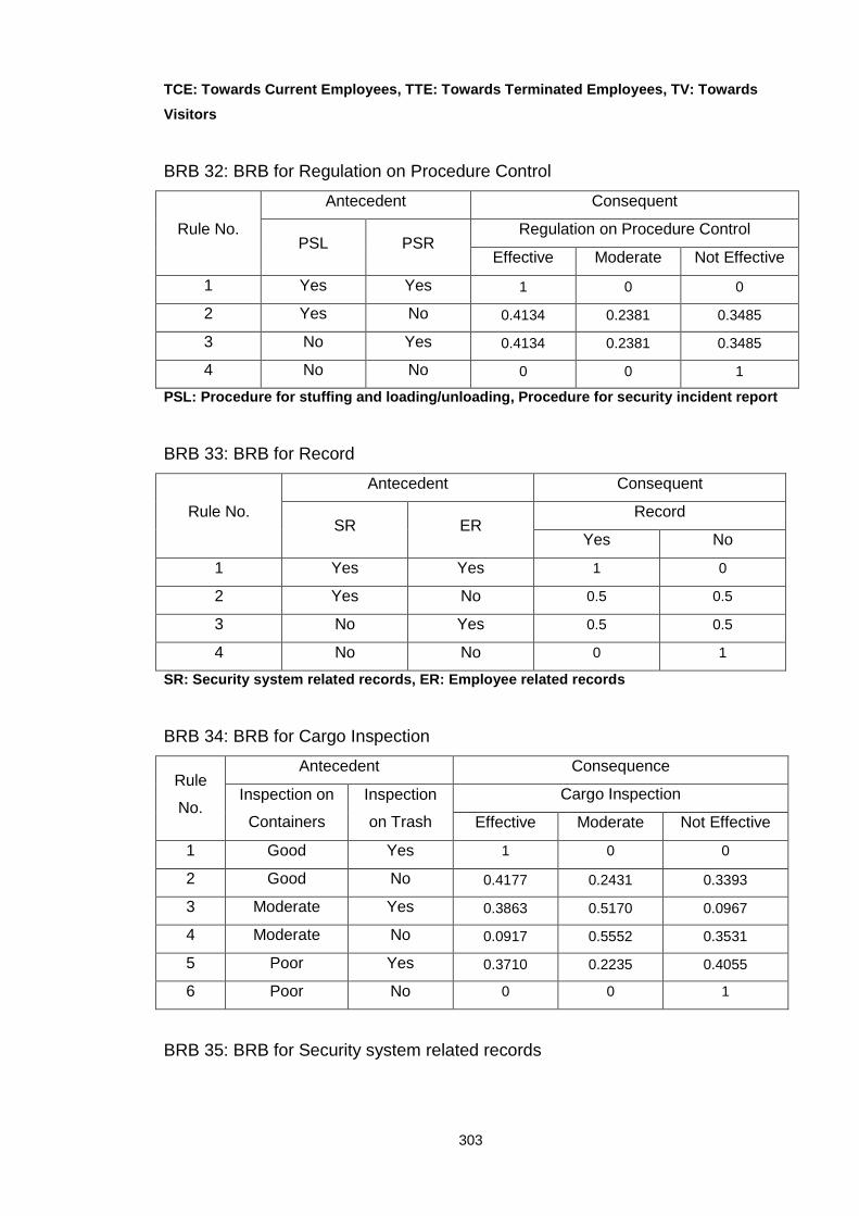
303
TCE: Towards Current Employees, TTE: Towards Termin ated Employees, TV: Towards
Visitors
BRB 32: BRB for Regulation on Procedure Control
Rule No.
Antecedent Consequent
PSL PSR Regulation on Procedure Control
Effective Moderate Not Effective
1 Yes Yes 1 0 0
2 Yes No 0.4134 0.2381 0.3485
3 No Yes 0.4134 0.2381 0.3485
4 No No 0 0 1
PSL: Procedure for stuffing and loading/unloading, Procedure for security incident report
BRB 33: BRB for Record
Rule No.
Antecedent Consequent
SR ER Record
Yes No
1 Yes Yes 1 0
2 Yes No 0.5 0.5
3 No Yes 0.5 0.5
4 No No 0 1
SR: Security system related records, ER: Employee r elated records
BRB 34: BRB for Cargo Inspection
Rule
No.
Antecedent Consequence
Inspection on
Containers
Inspection
on Trash
Cargo Inspection
Effective Moderate Not Effective
1 Good Yes 1 0 0
2 Good No 0.4177 0.2431 0.3393
3 Moderate Yes 0.3863 0.5170 0.0967
4 Moderate No 0.0917 0.5552 0.3531
5 Poor Yes 0.3710 0.2235 0.4055
6 Poor No 0 0 1
BRB 35: BRB for Security system related records

304
Rule No.
Antecedent Consequent
LAS LACS SR
Yes No
1 Yes Yes 1 0
2 Yes No 0.5 0.5
3 No Yes 0.5 0.5
4 No No 0 1
LAS: Logs of Alarm System, LACS: Logs of Access Con trol System, SR: Security system
related records
BRB 36: BRB for Employee related records
Rule No.
Antecedent Consequent
REC RT RTE Employee related records
Yes No
1 Yes Yes Yes 1 0
2 Yes Yes No 0.6333 0.3667
3 Yes No Yes 0.6333 0.3667
4 Yes No No 0.3667 0.6333
5 No Yes Yes 0.6333 0.3667
6 No Yes No 0.3667 0.6333
7 No No Yes 0.3667 0.6333
8 No No No 0 1
REC: Records on Emergency Contact, RT: Records on T raining, RTE: Records on
terminated employees in recent 3 years
305
Appendix 8 Publications Relevant to the Thesis
[1]. D.W. Tang, J. B. Yang and D. L. Xu, “Different aggregation patterns in Multi
Criteria Decision Making with application in security evaluation for Container
Supply Chains”, the 21st International Conference on Multiple Criteria Decision
Making, Jyväskylä, Finland, June 13th -17th, 2011.
[2]. D.W. Tang, D. L. Xu, S.L. Yang and J. B. Yang, “Evaluation based
Resource Allocation to Improve Security in Container Line Supply Chain”, the
19th Conference of the International Federation of Operational Research
Societies, Melbourne, Australia, July 10th – 15th, 2011.
[3]. D.W. Tang, D.L. Xu, J.B. Yang and Y.W. Chen, “A model for security
evaluation of a port storage area against theft in a Container Line Supply Chain”,
Joint Conference of the 4th International Conference of Operations and Supply
Chain Management and The 15th Asia Pacific Decision Sciences Institute,
Hong Kong & Guangzhou, China, 25 – 31 July 2010.
[4]. D.W. Tang, D.L. Xu, J.B. Yang and K.S. Chin, “A Bayesian network model
with a probability generation approach to evaluate risks in new product
development project”, the 14th International Conference on Automation and
Computing, Brunel, England, 6 September 2008.
[5]. K.S. Chin, D.W. Tang, J.B. Yang, S.Y. Wong and H.W. Wang, “Assessing
New Product Development Project Risk by Bayesian Network with a Systematic
Probability Generation Methodology”, Expert Systems with Applications, Vol. 36,
No. 6, pp. 9879-9890, 2009 (Note: First author is the supervisor)
Note: among the publications, [1] is corresponding to Chapter 6 of the thesis, [2]
is corresponding to Chapter 5 of the thesis, [3] is corresponding to Chapter 3 of
the thesis, while [4] and [5] are corresponding to Chapter 4 of the thesis. In
addition, a paper corresponding to Chapter 7 is drafted for submission to a high
quality journal.