Contact Details Distributed Source Coding: Theory and Practice · coding (NC) SW coding WZ coding...

1

Distributed Source Coding:Theory and Practice

EUSIPCO’08Lausanne, Switzerland

August 25 2008

Speakers: Dr Vladimir Stankovic, Dr Lina Stankovic, Dr Samuel Cheng

Contact Details

• Vladimir Stanković� Department of Electronic and Electrical Engineering, University of

Strathclyde� Email: [email protected]� Web: http://personal.strath.ac.uk/vladimir.stankovic

• Lina Stanković� Department of Electronic and Electrical Engineering, University of

Strathclyde� Email: [email protected]� Web: http://personal.strath.ac.uk/lina.stankovic

• Samuel Cheng� Department of Electrical and Computer Engineering, University of

Oklahoma� Email: [email protected]� Web: http://faculty-staff.ou.edu/C/Szeming.Cheng-1/

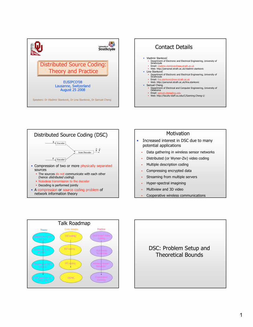
Distributed Source Coding (DSC)

• Compression of two or more physically separatedsources� The sources do not communicate with each other

(hence distributed coding)

� Noiseless transmission to the decoder

� Decoding is performed jointly

• A compression or source coding problem of network information theory

EncoderX

EncoderY

Joint DecoderX Y^ ^

• Increased interest in DSC due to many potential applications

� Data gathering in wireless sensor networks

� Distributed (or Wyner-Ziv) video coding

� Multiple description coding

� Compressing encrypted data

� Streaming from multiple servers

� Hyper-spectral imagining

� Multiview and 3D video

� Cooperative wireless communications

Motivation

Talk Roadmap

Slepian-Wolf (SW) problem

Wyner-Ziv (WZ) problem

Multiterminal (MT)problem

DSC and Network coding (NC)

SW coding

WZ coding

MT coding

DS-NC

Wireless Sensor Networks

Distributed Video Coding

Cooperative Diversity

Multimedia Streaming

Theory Code designs Practice

DSC: Problem Setup and Theoretical Bounds

2

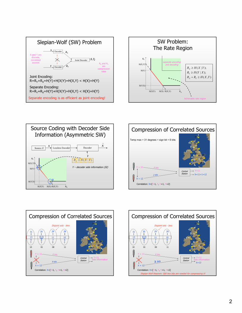
Slepian-Wolf (SW) Problem

EncoderX

EncoderY

Joint DecoderY),(X ˆˆ

RX

RY

Joint Encoding: R=RY+RX=H(Y)+H(X|Y)=H(X,Y) < H(X)+H(Y)

Separate encoding is as efficient as joint encoding!

Separate Encoding: R=RY+RX=H(Y)+H(X|Y)=H(X,Y) < H(X)+H(Y)

RX and RY

are compression

rates

X and Y are discrete,

correlated sources

SW Problem: The Rate Region

),(

);|(

);|(

YXHRR

XYHR

YXHR

YX

Y

X

≥+

≥

≥

RX

H(Y|X)

H(X)

H(Y)

H(X|Y)

RY

H(X,Y)

H(X,Y)

Achievable rate region

separate encoding and decoding

Source Coding with Decoder Side Information (Asymmetric SW)

Lossless EncoderSource XX

DecoderX^

Y

RX

H(Y|X)

H(X)

H(Y)

H(X|Y)

RY

H(X,Y)

H(X,Y)

A

B

)|( YXHRX ≥

Y – decoder side information (SI)

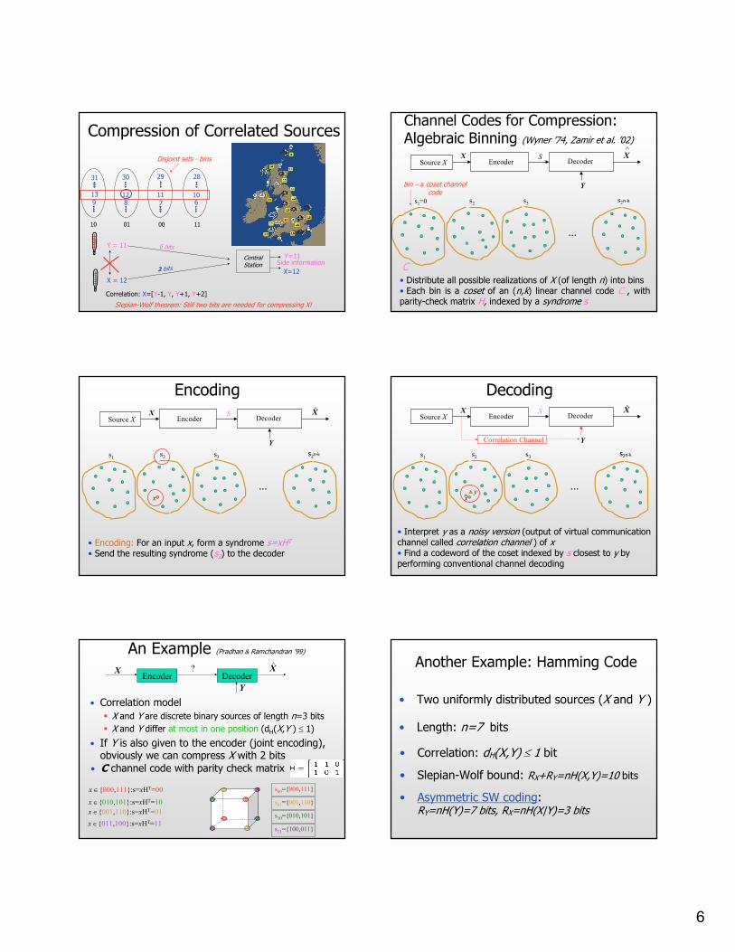
Compression of Correlated Sources

Y = 11

X = 12

CentralStation

Correlation: X=[Y-1, Y, Y+1, Y+2]

6 bits

2 bits

Y=11

X=11+1=12

Temp max = 31 degrees + sign bit = 6 bits


Y = 11

X = 12

CentralStation

6 bits

? bits

Y=11


Side information

10

30 29 28

13 12 11 109 8 7 6

01 00 11

31

Disjoint sets - bins


Y = 11

X = 12

CentralStation

6 bits

2 bits

Y=11

Slepian-Wolf theorem: Still two bits are needed for compressing X!


X=12

Side information

10

30 29 28

13 12 11 109 8 7 6

01 00 11

31

Disjoint sets - bins

3

X1X2

Encoder

Encoder

X1

X2

Decoder

Slepian-Wolf network (Slepian & Wolf ’73)

Encoder

Encoder

X1

X2

Decoder

Slepian-Wolf-Cover network (Wolf ’74, Cover ’75)

Encoder

Encoder

X3

X4

Encoder

Encoder

X1

X2

Encoder

Encoder

X3

X4

Network

Decoder

Decoder

X1 X2

X3

Uncorrelated sources over network (Ahlswede et al. ’00)

X4

X1 X2

X3 X4

X1 X2

X3 X4

Encoder

Encoder

X1

X2

Decoder

Lossless multiterminal network (Csiszár & Körner ’80, Han & Kobayashi ’80)

Encoder

Encoder

X3

X4

X2Decoder X3 X4

X1 X2 X3

X1X2

Encoder

Encoder

X1

X2

Decoder

Slepian-Wolf network (Slepian & Wolf ’73)

Encoder

Encoder

X1

X2

Decoder

Slepian-Wolf-Cover network (Wolf ’74, Cover ’75)

Encoder

Encoder

X3

X4

Encoder

Encoder

X1

X2

Encoder

Encoder

X3

X4

Network

Decoder

Decoder

X1 X2

X3

Correlated sources over network (Song & Yeung ’01)

X4

X1 X2

X3 X4

X1 X2

X3 X4

Encoder

Encoder

X1

X2

Decoder

Encoder

Encoder

X3

X4

X2Decoder X3 X4

X1 X2 X3

Lossless multiterminal network (Csiszár & Körner ’80, Han & Kobayashi ’80)

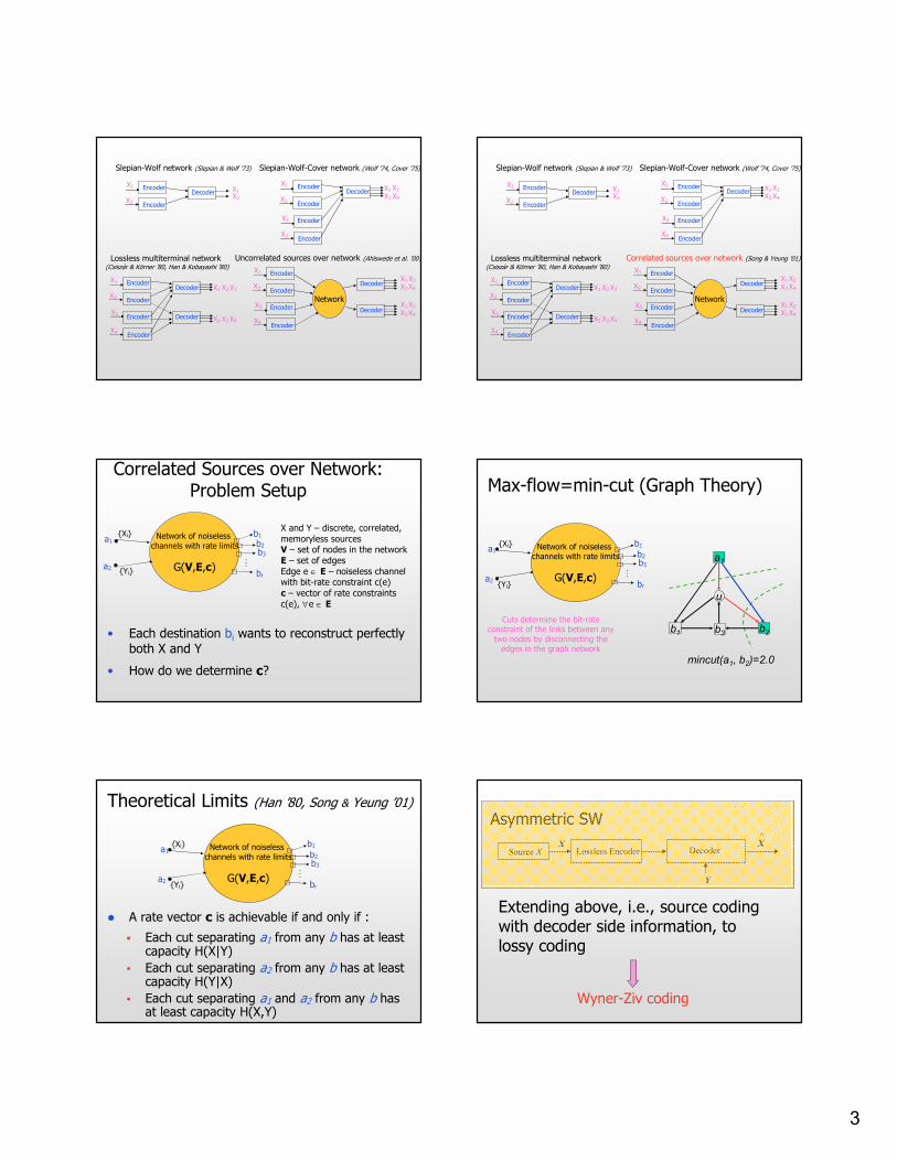
Correlated Sources over Network: Problem Setup

Network of noiseless channels with rate limits

G(V,E,c)

b1

b2

b3

br

a1

a2

...

{Xi}

{Yi}

X and Y – discrete, correlated, memoryless sourcesV – set of nodes in the networkE – set of edgesEdge e ∈ E – noiseless channel with bit-rate constraint c(e) c – vector of rate constraints c(e), ∀e ∈ E

• Each destination bi wants to reconstruct perfectly both X and Y

• How do we determine c?

Max-flow=min-cut (Graph Theory)

b3b1 b2

a1

u

mincut(a1, b2)=2.0


G(V,E,c)

b1

b2

b3

br

a1

a2

...

{Xi}

{Yi}

Cuts determine the bit-rate constraint of the links between any

two nodes by disconnecting the edges in the graph network

Theoretical Limits (Han ’80, Song & Yeung ’01)

� A rate vector c is achievable if and only if :

� Each cut separating a1 from any b has at least capacity H(X|Y)

� Each cut separating a2 from any b has at least capacity H(Y|X)

� Each cut separating a1 and a2 from any b has at least capacity H(X,Y)


G(V,E,c)

b1

b2

b3

br

a1

a2

...

{Xi}

{Yi}

Extending above, i.e., source coding with decoder side information, to lossy coding

Wyner-Ziv coding


DecoderX^

Y

Asymmetric SW

4

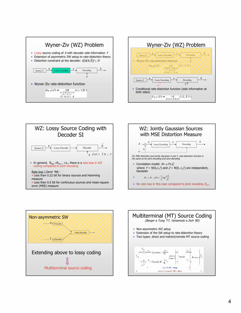
Wyner-Ziv (WZ) Problem

Lossy EncodingSource XX V

DecodingX̂

Y

• Wyner-Ziv rate-distortion function

• Lossy source coding of X with decoder side information Y• Extension of asymmetric SW setup to rate-distortion theory

• Distortion constraint at the decoder: E[d(X,X)] ≤ D^

Wyner-Ziv (WZ) Problem

Lossy EncodingSource XX V

DecodingX̂

Y• Wyner-Ziv rate-distortion function

• Conditional rate-distortion function (side information at both sides)

Source XX V X̂

YY

Lossy Encoding Decoding

WZ: Lossy Source Coding with Decoder SI

Lossy EncoderSource XX

DecoderX^

Y

Rate loss (Zamir ’96) :� Less than 0.22 bit for binary sources and Hamming measure� Less than 0.5 bit for continuous sources and mean-square error (MSE) measure

• In general, RWZ ≥RX|Y , i.e., there is a rate loss in WZ coding compared to joint encoding

WZ: Jointly Gaussian Sources with MSE Distortion Measure

•

Lossy EncodingX V

DecodingX̂

Y

Z

• Correlation model: X= αY+Z,

where Y ~ N(0,σY2) and Z ~ N(0, σZ

2) are independent, Gaussian

• No rate loss in this case compared to joint encoding RX|Y

α

DDRR Z

YXWZ

2

log2

1)(|

σ==

For MSE distortion and jointly Gaussian X and Y, rate-distortion function is the same as for joint encoding and joint decoding

Extending above to lossy coding

Multiterminal source coding

Non-asymmetric SW

EncoderX

EncoderY

Joint Decoder

Multiterminal (MT) Source Coding(Berger & Tung ’77, Yamamoto & Itoh ’80)

• Non-asymmetric WZ setup

• Extension of the SW setup to rate-distortion theory

• Two types: direct and indirect/remote MT source coding

5

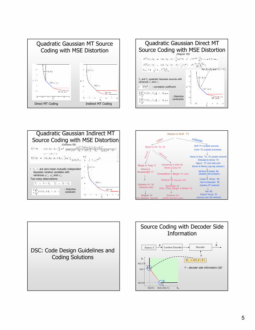
Quadratic Gaussian MT Source Coding with MSE Distortion

Direct MT Coding Indirect MT Coding

(Wagner ’05)

Quadratic Gaussian Direct MT Source Coding with MSE Distortion

Y1 and Y2 quadratic Gaussian sources with variances and 2

1yσ 2

2yσ

- correlation coefficient

- Distortion constraints

for D1=D2 and 2

2

2

1 yy σσ =

are zero-mean mutually independent Gaussian random variables with variances , and .

Two noisy observations:

(Oohama ’05)

Quadratic Gaussian Indirect MT Source Coding with MSE Distortion

2

2nσ2

xσ 2

1nσ

- Distortion constraint

Slepian & Wolf ’73

Wyner & Ziv ’76, ’78

Berger & Tung ’77

Omura &

Housewright ’77

Oohama ’97, ’05(Gaussian case)

Yamamoto & Itoh ’80

Flynn & Gray ’87

Viswanathan & Berger ’97 (CEO)

Oohama ’98 (Gaussian CEO)

Viswanath ’02Chen, Zhao, Berger & Wicker ’03

Direc

t M

T Indirect MT Wyner & Gray ’74, ’75 (simple network)

Ahlswede & Körner ’75

Sgarro ’77 (two-help-one)

Körner & Marton (zig-zag network )

Gel’fand & Pinsker ’80(lossless CEO problem)

Csiszár & Körner ’80

Han & Kobayashi ’80

(lossless MT network)

Oohama ’05 (Jointly Gaussian case)

LOSSY LOSSLESS

Wolf ’74 (multiple sources)

Cover ’75 (ergodic processes)

Han ’80

Song & Yeung ’01

(sources over the network)Wagner ’05

(two Gaussian sources)

DSC: Code Design Guidelines and Coding Solutions

Source Coding with Decoder Side Information

RX

H(Y|X)

H(X)

H(Y)

H(X|Y)

RY

H(X,Y)

H(X,Y)

A

B

)|( YXHRX ≥


DecoderX^

Y

Y – decoder side information (SI)

6


Y = 11

X = 12

CentralStation

6 bits

2 bits

Y=11

Slepian-Wolf theorem: Still two bits are needed for compressing X!


X=12

Side information

10

30 29 28

13 12 11 109 8 7 6

01 00 11

31

Disjoint sets - bins EncoderSource XX S

DecoderX^

Y

Channel Codes for Compression: Algebraic Binning (Wyner ’74, Zamir et al. ’02)

• Distribute all possible realizations of X (of length n) into bins• Each bin is a coset of an (n,k) linear channel code C , with parity-check matrix H, indexed by a syndrome s

bin – a coset channel code

s1=0 s2 s3

…

s2n-k

C

Encoding

• Encoding: For an input x, form a syndrome s=xHT

• Send the resulting syndrome (s2) to the decoder

EncoderSource XX S

DecoderX̂

Y

s1s2 s3

x

…

s2n-k

Decoding

• Interpret y as a noisy version (output of virtual communication channel called correlation channel ) of x• Find a codeword of the coset indexed by s closest to y by performing conventional channel decoding

EncoderSource XX S

DecoderX̂

YCorrelation Channel

s1s2 s3

x

…

s2n-k

y^

• Correlation model� X and Y are discrete binary sources of length n=3 bits

� X and Y differ at most in one position (dH(X,Y ) ≤ 1)

• If Y is also given to the encoder (joint encoding), obviously we can compress X with 2 bits

An Example (Pradhan & Ramchandran ’99)

Encoder DecoderX ?

Y

X^

• C channel code with parity check matrix

x ∈{000,111}:s=xHT=00

x ∈{001,110}:s=xHT=01

x ∈{010,101}:s=xHT=10

x ∈{011,100}:s=xHT=11

s00={000,111}

s10={010,101}

s01={001,110}

s11={100,011}

Another Example: Hamming Code

• Two uniformly distributed sources (X and Y )

• Length: n=7 bits

• Slepian-Wolf bound: RX+RY=nH(X,Y)=10 bits

• Correlation: dH(X,Y) ≤ 1 bit

• Asymmetric SW coding: RY=nH(Y)=7 bits, RX=nH(X|Y)=3 bits

7

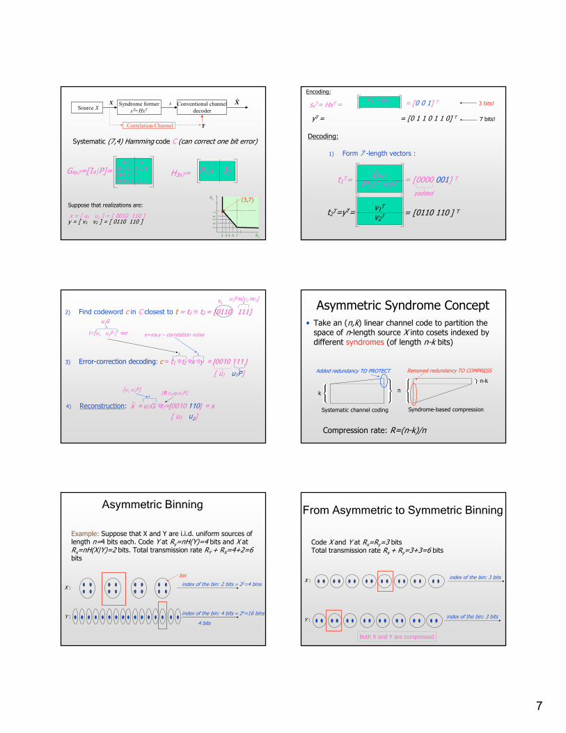
Syndrome former

sT=HxTSource XX s Conventional channel

decoder

X̂

YCorrelation Channel

Systematic (7,4) Hamming code C (can correct one bit error)

G4x7=[I4 P]=1 0 0 0 1 0 10 1 0 0 1 1 00 0 1 0 1 1 10 0 0 1 0 1 1

H33x7= P4x3T

I3

x = [ u1 u2 ] = [ 0010 110 ]y = [ v1 v2 ] = [ 0110 110 ]

Suppose that realizations are:

3 4 5 6 7

7 6

5 4

3

(3,7)

Rx

Ry

Encoding:

sxT= HxT = = [0 0 1] T

yT = = [0 1 1 0 1 1 0] T

3 bits!

7 bits!

PTu1T u2T

1) Form 7 -length vectors :

t1T=O4x1

PTu1T u2T = [0000 001] T

t2T=yT=v1T

v2T = [0110 110 ] T

Decoding:

padded

4) Reconstruction:: x = ux = u11G tG t11=[0010 =[0010 110110] = x] = x^

3)3) ErrorError--correction decodingcorrection decoding:: cc == tt11 tt2 2 xx y = [0010 111 ]y = [0010 111 ]

[ u1 u1P]

2) Find codeword c in C closest to tt = t= t11 tt2 2 = [0110 111]= [0110 111]

vv11u1P [u2 v2]

t=[u1 u1P ] e e=x y – correlation noise

[u1 u1P][0 u2 u1P]

[ u1 u2]

uu11GG

Asymmetric Syndrome Concept• Take an (n,k) linear channel code to partition the

space of n-length source X into cosets indexed by different syndromes (of length n-k bits)

nk

n-k

Systematic channel coding Syndrome-based compression

Compression rate: R=(n-k)/n

Added redundancy TO PROTECT Removed redundancy TO COMPRESS

Asymmetric Binning

Example:Example: Suppose that X and Y are i.i.d. uniform sources of length n=4 bits each. Code Y at Ry=nH(Y)=4 bits and X at Rx=nH(X|Y)=2 bits. Total transmission rate RY + RX=4+2=6bits

X :

bin

Y :

index of the bin: 2 bits ≡ 22=4 bins

index of the bin: 4 bits ≡ 24=16 bins

4 bits

X :

Y :

Code X and Y at Rx=Ry=3 bitsTotal transmission rate Rx + Ry=3+3=6 bits

index of the bin: 3 bits

index of the bin: 3 bits

From Asymmetric to Symmetric Binning

Both X and Y are compressed

8

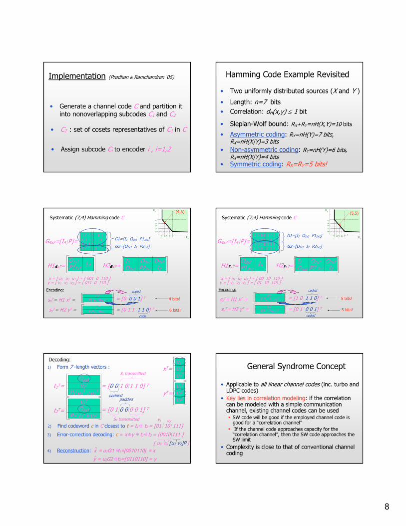
Implementation (Pradhan & Ramchandran ‘05)

• Generate a channel code C and partition it into nonoverlapping subcodes C1 and C2

• C2 : set of cosets representatives of C1 in C

• Assign subcode Ci to encoder i , i=1,2

Hamming Code Example Revisited

• Two uniformly distributed sources (X and Y )

• Length: n=7 bits

• Slepian-Wolf bound: RX+RY=nH(X,Y)=10 bits

• Correlation: dH(x,y) ≤ 1 bit

• Asymmetric coding: RY=nH(Y)=7 bits, RX=nH(X|Y)=3 bits

• Symmetric coding: RX=RY=5 bits!

• Non-asymmetric coding: RY=nH(Y)=6 bits, RX=nH(X|Y)=4 bits

G4x7=[I4 P]=1 0 0 0 1 0 10 1 0 0 1 1 00 0 1 0 1 1 10 0 0 1 0 1 1

G1=[I3 O3x1 P13x3]

G2=[O1x3 I1 P21x3]

H144x7=O1x3

P13x3T I4 H266x7=

I3 O3x1 O3x3

O3x3 P23x1 I3T

3 4 5 6 7

7 6

5 4

3

Systematic (7,4) Hamming code C

x = [ u1 u2 u3 ] = [ 001 0 110 ]y = [ v1 v2 v3 ] = [ 011 0 110 ]

Encoding:

sxT= H1 xT = = [0 0 0 1] T

syT= H2 yT =v1T

P2Tv2T v3T = [0 1 1 1 1 0] T

4 bits!

6 bits!

u2T

P1Tu1T u3T

(4,6)

Rx

Ry

coded

coded

G4x7=[I4 P]=1 0 0 0 1 0 10 1 0 0 1 1 00 0 1 0 1 1 10 0 0 1 0 1 1

G1=[I2 O2x2 P12x3]

G2=[O2x2 I2 P22x3]

H15x7=O2x2

P13x2T I5 H25x7=

I2 O2x2 O2x3

O3x2 P2 3x2 I3T

(5,5)

3 4 5 6 7

7 6

5 4

3

Systematic (7,4) Hamming code C

x = [ u1 u2 u3 ] = [ 00 10 110 ]y = [ v1 v2 v3 ] = [ 01 10 110 ]

Rx

Ry

Encoding:

sxT= H1 xT = = [1 0 1 1 0] T

syT= H2 yT =v1T

P2Tv2T v3T = [0 1 0 0 1] T

5 bits!

5 bits!

u2T

P1Tu1T u3T

coded

coded

1) Form 7 -length vectors :

t1T=O2x1

u2T

P1Tu1T u3T= [0 0 1 0 1 1 0] T

t2T=

v1T

O2x1

P2Tv2T v3T= [0 1 0 0 0 0 1] T

Decoding:

4) Reconstruction:: x = ux = u11G1 tG1 t11=[0010110] = x=[0010110] = x

y = uy = u22G2 tG2 t22=[0110110] = y=[0110110] = y^

^

u1T

u2T

u3TxT=

v1T

v2T

v3TyT=

Sx transmitted

paddedpadded

SY transmitted

3) Error-correction decoding: c = x y t1 t2 = [0010 111 ]

[ u1 v2 [u1 v2]P ]

2) Find codeword c in C closest to tt = t= t11 tt2 2 = [01 10 111]= [01 10 111]

vv11 uu22

General Syndrome Concept

• Applicable to all linear channel codes (inc. turbo and LDPC codes)

• Key lies in correlation modeling: if the correlation can be modeled with a simple communication channel, existing channel codes can be used� SW code will be good if the employed channel code is

good for a “correlation channel”

� If the channel code approaches capacity for the “correlation channel”, then the SW code approaches the SW limit

• Complexity is close to that of conventional channel coding

9

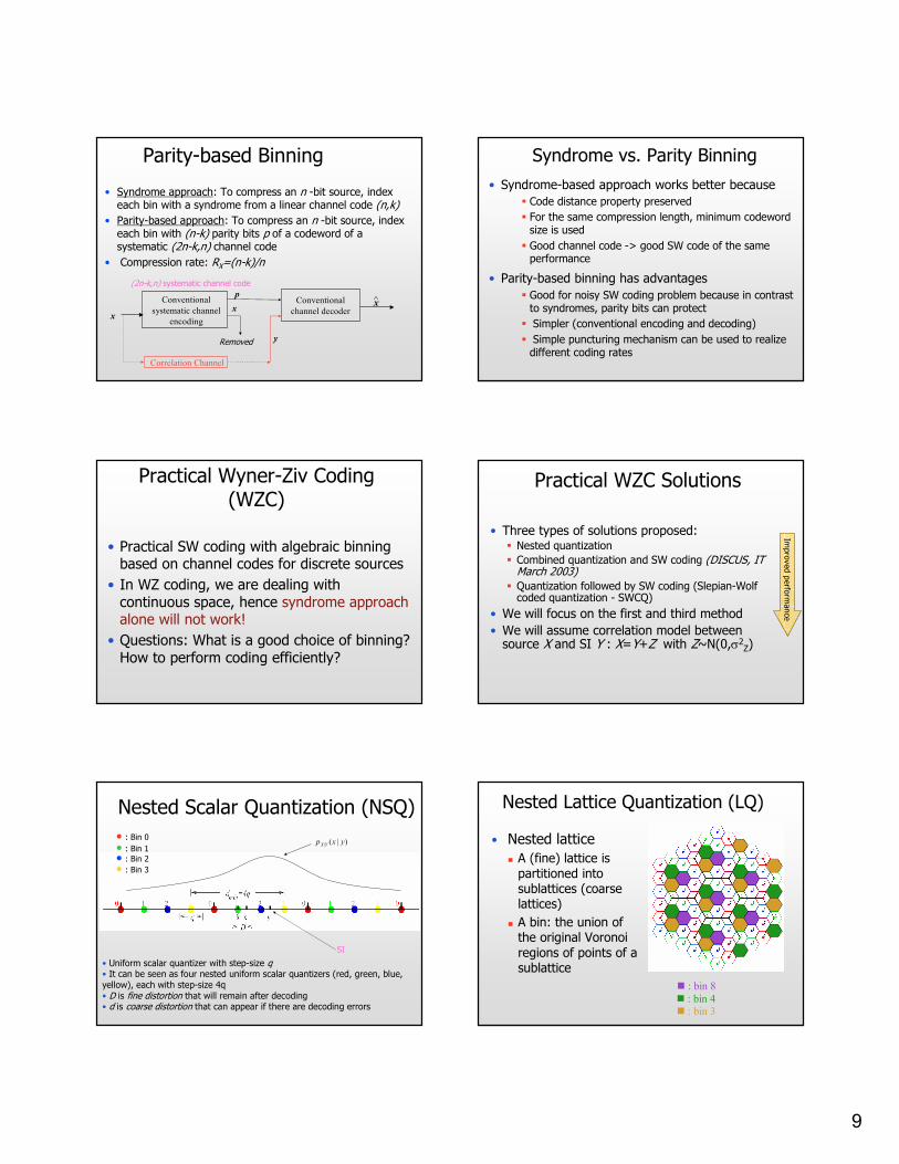
Parity-based Binning

• Syndrome approach: To compress an n -bit source, index each bin with a syndrome from a linear channel code (n,k)

• Parity-based approach: To compress an n -bit source, index each bin with (n-k) parity bits p of a codeword of a systematic (2n-k,n) channel code

• Compression rate: RX=(n-k)/n

Conventional

systematic channel

encodingx

Conventional

channel decoderx̂

y

Correlation Channel

p

x

Removed

(2n-k,n) systematic channel code

Syndrome vs. Parity Binning

• Syndrome-based approach works better because� Code distance property preserved

� For the same compression length, minimum codeword size is used

� Good channel code -> good SW code of the same performance

• Parity-based binning has advantages� Good for noisy SW coding problem because in contrast

to syndromes, parity bits can protect

� Simpler (conventional encoding and decoding)

� Simple puncturing mechanism can be used to realize different coding rates

• Practical SW coding with algebraic binning based on channel codes for discrete sources

• In WZ coding, we are dealing with continuous space, hence syndrome approach alone will not work!

• Questions: What is a good choice of binning? How to perform coding efficiently?

Practical Wyner-Ziv Coding (WZC)

• Three types of solutions proposed: � Nested quantization

� Combined quantization and SW coding (DISCUS, IT March 2003)

� Quantization followed by SW coding (Slepian-Wolf coded quantization - SWCQ)

• We will focus on the first and third method

• We will assume correlation model between source X and SI Y : X=Y+Z with Z~N(0,σ2

Z)

Practical WZC Solutions

Impro

ved p

erfo

rmance

Nested Scalar Quantization (NSQ)

• Uniform scalar quantizer with step-size q• It can be seen as four nested uniform scalar quantizers (red, green, blue, yellow), each with step-size 4q• D is fine distortion that will remain after decoding• d is coarse distortion that can appear if there are decoding errors

SI

• : Bin 0

• : Bin 1• : Bin 2

• : Bin 3

)|(| yxp YX

Nested Lattice Quantization (LQ)

• Nested lattice

� A (fine) lattice is partitioned into sublattices (coarse lattices)

� A bin: the union of the original Voronoiregions of points of a sublattice

� : bin 8

� : bin 4

� : bin 3

10

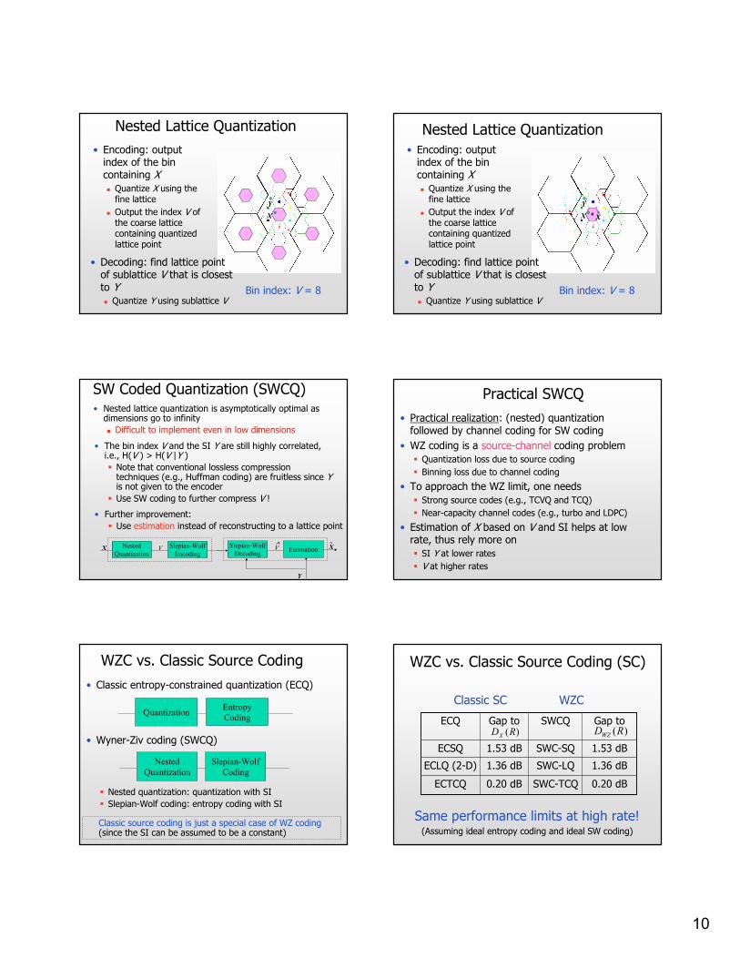
• Encoding: output index of the bin containing X� Quantize X using the

fine lattice

� Output the index V of the coarse lattice containing quantized lattice point

Y

Nested Lattice Quantization

• Decoding: find lattice point of sublattice V that is closest to Y� Quantize Y using sublattice V

Bin index: V = 8

X

Y

Nested Lattice Quantization

Bin index: V = 8

X^X

• Encoding: output index of the bin containing X� Quantize X using the

fine lattice

� Output the index V of the coarse lattice containing quantized lattice point

• Decoding: find lattice point of sublattice V that is closest to Y� Quantize Y using sublattice V

SW Coded Quantization (SWCQ)• Nested lattice quantization is asymptotically optimal as

dimensions go to infinity

� Difficult to implement even in low dimensions

Nested

Quantization

Slepian-Wolf

Encoding

Slepian-Wolf

DecodingEstimationV V

Y

X X^

• The bin index V and the SI Y are still highly correlated, i.e., H(V ) > H(V |Y ) � Note that conventional lossless compression

techniques (e.g., Huffman coding) are fruitless since Yis not given to the encoder

� Use SW coding to further compress V !

• Further improvement:

� Use estimation instead of reconstructing to a lattice point

^

Practical SWCQ

• Practical realization: (nested) quantization followed by channel coding for SW coding

• WZ coding is a source-channel coding problem� Quantization loss due to source coding

� Binning loss due to channel coding

• To approach the WZ limit, one needs � Strong source codes (e.g., TCVQ and TCQ)

� Near-capacity channel codes (e.g., turbo and LDPC)

• Estimation of X based on V and SI helps at low rate, thus rely more on� SI Y at lower rates

� V at higher rates

WZC vs. Classic Source Coding

• Classic entropy-constrained quantization (ECQ)

• Wyner-Ziv coding (SWCQ)

� Nested quantization: quantization with SI

� Slepian-Wolf coding: entropy coding with SI

QuantizationEntropy

Coding

Nested

Quantization

Slepian-Wolf

Coding

Classic source coding is just a special case of WZ coding(since the SI can be assumed to be a constant)

0.20 dBSWC-TCQ0.20 dBECTCQ

1.36 dBSWC-LQ1.36 dBECLQ (2-D)

1.53 dBSWC-SQ1.53 dBECSQ

Gap toSWCQGap to ECQ)(RDX

)(RDWZ

Classic SC WZC

Same performance limits at high rate!(Assuming ideal entropy coding and ideal SW coding)

WZC vs. Classic Source Coding (SC)

11

1V

1( ', )y V2V

'y

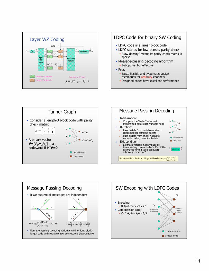
Layer WZ Coding

Q(.)X

1 1( ', ,..., )ny V V −

nV

CombineBitplane

SplitBit-

plane⋯

EstimateV̂V X̂

: binary SW encoder

: binary SW decoder1 1( ', ,..., )ky y V V −=

Side info at kth level

SWC

LDPC Code for binary SW Coding

• LDPC code is a linear block code

• LDPC stands for low-density parity-check� “Low-density” means its parity-check matrix is

sparse

• Message-passing decoding algorithm� Suboptimal but effective

• Pros� Exists flexible and systematic design

techniques for arbitrary channels

� Designed codes have excellent performance

Tanner Graph

V1+V2+V3

V1+V2

V1

V2

V3

: variable node

: check node

• Consider a length-3 block code with parity check matrix

• A binary vector V=[V1,V2,V3] is a codeword if HTV=0

Message Passing Decoding

1. Initialization:� Compute the “belief” of actual

transmitted bit at each variable node

2. Iteration:� Pass beliefs from variable nodes to

check nodes; combine beliefs� Pass beliefs from check nodes to

variable nodes; combine beliefs

3. Exit condition:� Estimate variable node values by

thresholding current beliefs. Exit if the estimates form a valid codeword; otherwise, back to 2.

Belief usually in the form of log-likelihood ratio

: variable node

: check node

channelV Y

V3

V2

V1

==

)1|(

)0|(log

Vyp

Vyp

• If we assume all messages are independent


• Message passing decoding performs well for long block-length code with relatively few connections (low-density)

y

21)1|(

)0|(log mm

Vyp

Vyp++

==

=Ψ 1 2tanh tanh tanh2 2 2

m mΦ=

SW Encoding with LDPC Codes

• Encoding:� Output check values S

• Compression rate: � R=(n-k)/n = 4/6 = 2/3

1

1

1

0

1

0

1

0

uncompressed

binary source

compressed

output

(syndrome)

0

1

: variable node

: check node

V

S

12

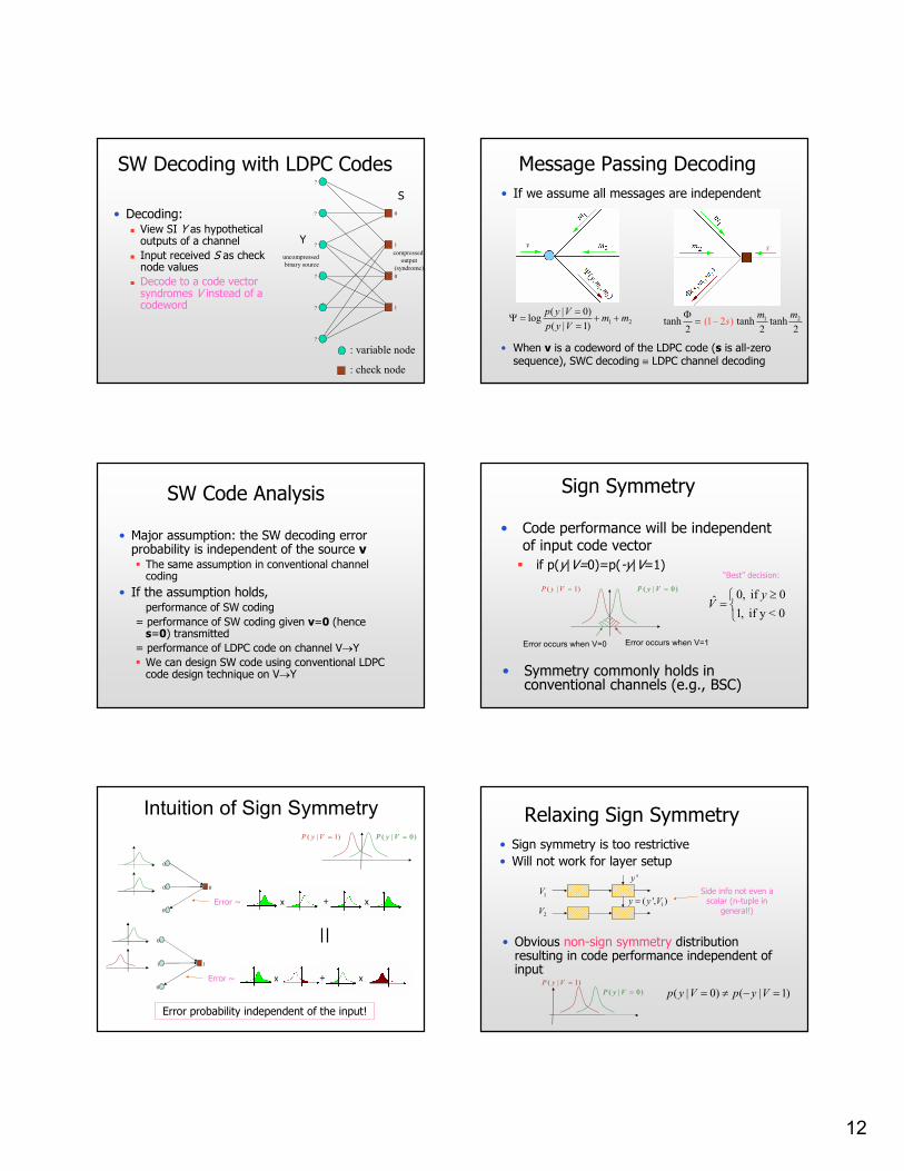
SW Decoding with LDPC Codes

• Decoding:� View SI Y as hypothetical

outputs of a channel

� Input received S as check node values

� Decode to a code vector syndromes V instead of a codeword

?

?

?

?

?

?

1

0

uncompressed

binary source

compressed

output

(syndrome)

0

1

: variable node

: check node

Y

S • If we assume all messages are independent


• When v is a codeword of the LDPC code (s is all-zero sequence), SWC decoding ≡ LDPC channel decoding

y

21)1|(

)0|(log mm

Vyp

Vyp++

==

=Ψ

s

tanh2

Φ= (1 2 )s− 1 2tanh tanh

2 2

m m

SW Code Analysis

• Major assumption: the SW decoding error probability is independent of the source v� The same assumption in conventional channel

coding

• If the assumption holds,performance of SW coding

= performance of SW coding given v=0 (hence s=0) transmitted

= performance of LDPC code on channel V→Y

� We can design SW code using conventional LDPC code design technique on V→Y

Sign Symmetry

• Code performance will be independent of input code vector

� if p(y|V=0)=p(-y|V=1)

)0|( =VyP)1|( =VyP

Error occurs when V=1Error occurs when V=0

• Symmetry commonly holds in conventional channels (e.g., BSC)

“Best” decision:

0, if 0

1, if y < ˆ

0

yV

≥=

Intuition of Sign Symmetry

0

0 0

Error ~ x + x

0

1 1

Error ~ x x

)1|( =VyP )0|( =VyP

+

Error probability independent of the input!

0

0

Relaxing Sign Symmetry

• Sign symmetry is too restrictive

• Will not work for layer setup

• Obvious non-sign symmetry distribution resulting in code performance independent of input

)1|( =VyP

)0|( =VyP

1V

1( ', )y y V=2V

'y

Side info not even a scalar (n-tuple in

general!)

(( )| | 10) p Vy V yp = ≠ − =

13

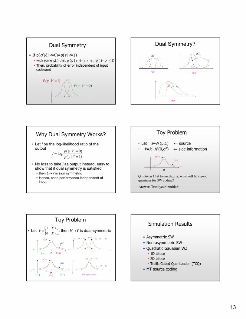
Dual Symmetry

• If p(g(y)|V=0)=p(y|V=1)

� with some g(•) that g (g (y ))=y (i.e., g (•)=g -1(•))

� Then, probability of error independent of input codeword

)1|( =VyP

)0|( =VyP

)(·g

Dual Symmetry?

)(·g

YES!YES!

)(·g

NO!

Why Dual Symmetry Works?

• Let l be the log-likelihood ratio of the output

• No loss to take l as output instead, easy to show that if dual symmetry is satisfied

� then L→Y is sign symmetric

� Hence, code performance independent of input

(log

(

0)

)

|

| 1

p y Vl

p y V

==

=

Toy Problem

• Let X~N (µ,1) ← source

• Y=X+N (0,σ2) ← side information

µ

p(x)

p(y)

Q.: Given 1 bit to quantize X, what will be a good

quantizer for SW coding?

Answer: Trust your intuition!

Toy Problem

• Let , then V→Y is dual-symmetric

<

≥=

µµ

X

XV

0

1

µ

p(x)

p(y)

V=1 V=0

)1|( =Vyp )0|( =Vyp)( ·g

µ

p(x)

p(y)

V=1 V=0 V=1

)1|( =Vyp

)0|( =Vyp

Not symmetric

Simulation Results

• Asymmetric SW

• Non-asymmetric SW

• Quadratic Gaussian WZ

� 1D lattice

� 2D lattice

� Trellis Coded Quantization (TCQ)

• MT source coding

14

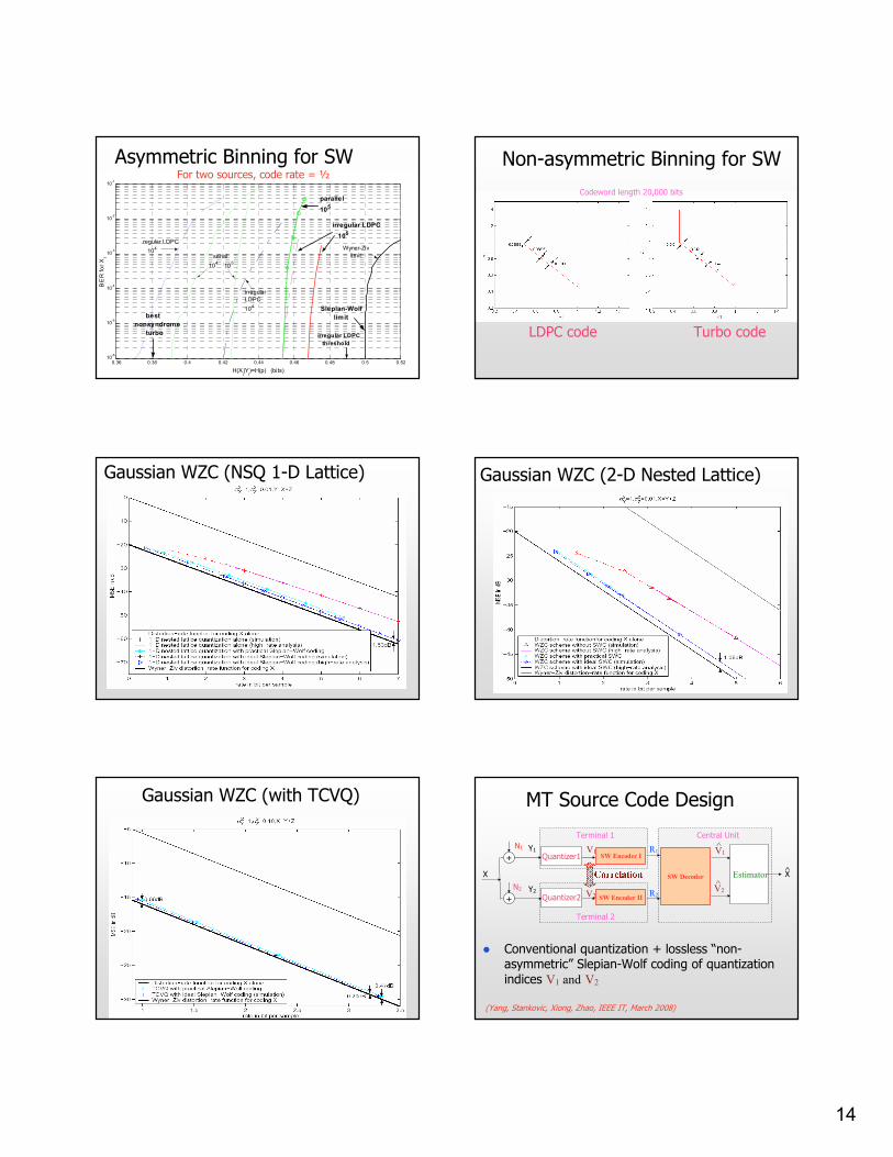
Asymmetric Binning for SW

0.36 0.38 0.4 0.42 0.44 0.46 0.48 0.5 0.5210

-6

10-5

10-4

10-3

10-2

10-1

H(Xi|Y

i)=H(p) (bits)

BE

R f

or

Xi

irregular

LDPC

104

regular LDPC

104

best

nonsyndrome

turbo

Slepian-Wolf

limit

irregular LDPC

105

parallel

105

irregular LDPC

threshold

Wyner-Ziv

limit serial

104 10

5

For two sources, code rate = ½Non-asymmetric Binning for SW

LDPC code Turbo code

Codeword length 20,000 bits

Gaussian WZC (NSQ 1-D Lattice)

1.53dB

Gaussian WZC (2-D Nested Lattice)

Gaussian WZC (with TCVQ)

Central UnitTerminal 1

MT Source Code Design

SW Encoder I

SW Encoder II

SW Decoder

R1

X

+

+

N1

N2

Quantizer1

Quantizer2

Y1

Y2

X^

V1

V2

Estimator

R2

V1

V2

Terminal 2

� Conventional quantization + lossless “non-asymmetric” Slepian-Wolf coding of quantization indices V1 and V2

(Yang, Stankovic, Xiong, Zhao, IEEE IT, March 2008)

^

^

15

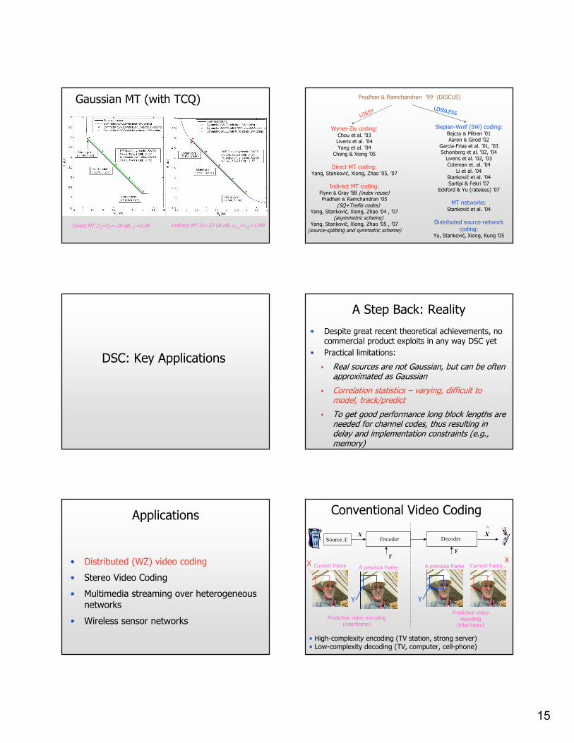
Gaussian MT (with TCQ)

Direct MT D1=D2=-30 dB, ρ=0.99 Indirect MT D=-22.58 dB, σn1=σn2=1/99

Slepian-Wolf (SW) coding:Bajcsy & Mitran ’01Aaron & Girod ’02

Garcia-Frias et al. ’01, ’03Schonberg et al. ’02, ’04

Liveris et al. ’02, ’03Coleman et. al. ’04

Li et al. ’04Stanković et al. ’04 Sartipi & Fekri ’07

Eckford & Yu (rateless) ’07

MT networks:Stanković et al. ’04

Distributed source-network coding:

Yu, Stanković, Xiong, Kung ’05

Pradhan & Ramchandran ’99 (DISCUS)

LOSSYLOSSLESS

Wyner-Ziv coding:Chou et al. ’03Liveris et al. ’04Yang et al. ’04

Cheng & Xiong ’05

Direct MT coding:Yang, Stanković, Xiong, Zhao ’05, ’07

Indirect MT coding:Flynn & Gray ’88 (index reuse)Pradhan & Ramchandran ’05

(SQ+Trellis codes)Yang, Stanković, Xiong, Zhao ’04 , ’07

(asymmetric scheme)Yang, Stanković, Xiong, Zhao ’05 , ’07

(source-splitting and symmetric scheme)

DSC: Key Applications

A Step Back: Reality

• Despite great recent theoretical achievements, no commercial product exploits in any way DSC yet

• Practical limitations:

� Real sources are not Gaussian, but can be often approximated as Gaussian

� Correlation statistics – varying, difficult to model, track/predict

� To get good performance long block lengths are needed for channel codes, thus resulting in delay and implementation constraints (e.g., memory)

Applications

• Distributed (WZ) video coding

• Stereo Video Coding

• Multimedia streaming over heterogeneous networks

• Wireless sensor networks

XX

• High-complexity encoding (TV station, strong server)• Low-complexity decoding (TV, computer, cell-phone)

Conventional Video Coding

EncoderSource XX

DecoderX^

Y

Predictive video encoding (interframe)

Predictive video decoding

(interframe)

Current frame A previous frame Current frame

Y

A previous frame

YY

16

Y

XX

• The encoder does not need to know SI Y

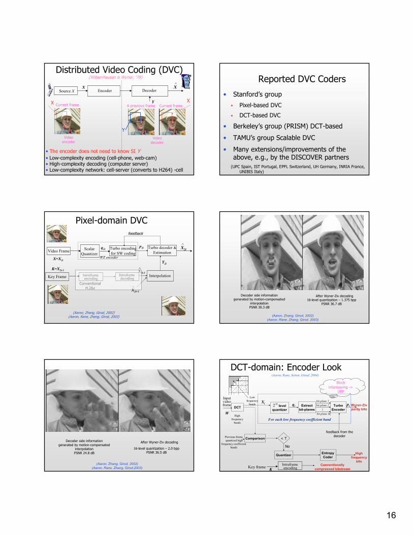
Distributed Video Coding (DVC)

EncoderSource XX

DecoderX^

Y

Videoencoder

Videodecoder

Current frame A previous frame

(Witsenhausen & Wyner, ‘78)

Current frame

• Low-complexity encoding (cell-phone, web-cam)• High-complexity decoding (computer server)• Low-complexity network: cell-server (converts to H264) -cell

Reported DVC Coders

• Stanford’s group

� Pixel-based DVC

� DCT-based DVC

• Berkeley’s group (PRISM) DCT-based

• TAMU’s group Scalable DVC

• Many extensions/improvements of the above, e.g., by the DISCOVER partners

(UPC Spain, IST Portugal, EPFL Switzerland, UH Germany, INRIA France, UNIBIS Italy)

Pixel-domain DVC

Scalar

QuantizerVideo Frame

X=X2i

Turbo decoder &

Estimation

X2i

^

Y2i

Turbo encoding

for SW codingWZ encoder

Interpolation

(Aaron, Zhang, Girod, 2002)(Aaron, Rane, Zhang, Girod, 2003)

Key Frame Intraframeencoding

Intraframedecoding

X2i-1

ConventionalH.26x

feedback

q2ip2i

K=X2i-1 ^

X2i+1

^

Decoder side informationgenerated by motion-compensated

interpolationPSNR 30.3 dB

After Wyner-Ziv decoding16-level quantization – 1.375 bpp

PSNR 36.7 dB

(Aaron, Zhang, Girod, 2002)

(Aaron, Rane, Zhang, Girod, 2003)

Decoder side informationgenerated by motion-compensated

interpolationPSNR 24.8 dB

After Wyner-Ziv decoding

16-level quantization – 2.0 bppPSNR 36.5 dB

(Aaron, Zhang, Girod, 2002)

(Aaron, Rane, Zhang, Girod,2003)

DCT-domain: Encoder Look(Aaron, Rane, Setton, Girod, 2004)

For each low frequency coefficient band

level

quantizerDCT

iM2 Turbo

Encoder

Extract

bit-planes

bit-plane 1

bit-plane 2

bit-plane Mi

…

Inputvideo frame

QuantizerEntropy

Coder

ComparisonPrevious-frame

quantized high

frequency coefficient

bands

Wyner-Ziv

parity bits

High

frequency

bits

Low

frequency

bands

feedback from the decoder

W

Xi qi

Key frameIntraframeencodingK

Conventionally

compressed bitstream

pi

Block interleaving ->

UEP

< T

High

frequency

bands

No

17

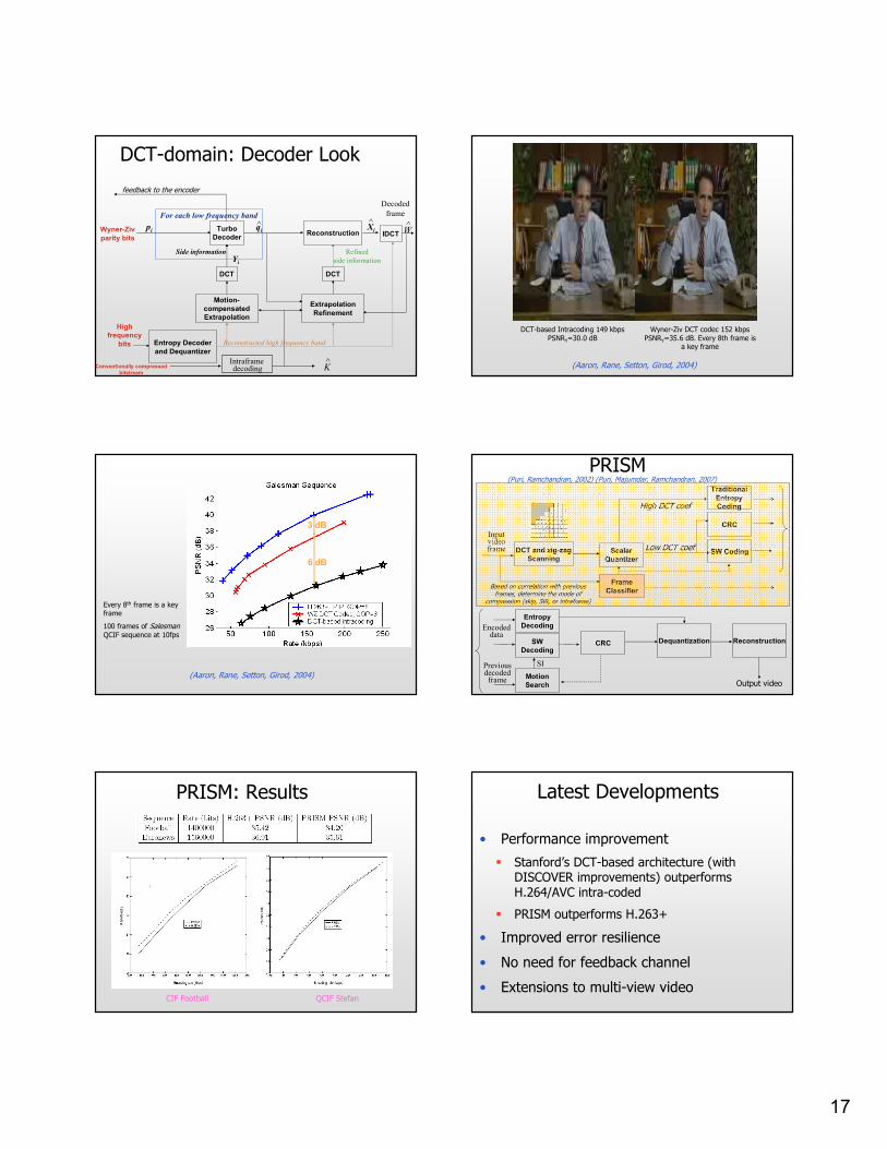
DCT-domain: Decoder Look

IDCTReconstruction

DCT

Entropy Decoder

and Dequantizer

Side information

Wyner-Ziv

parity bits

High

frequency

bits

Turbo

Decoder

Motion-

compensated

Extrapolation

DCT

Refined

side information

Extrapolation

Refinement

For each low frequency band

Decoded

frame

Reconstructed high frequency band

feedback to the encoder

pi qi^ ^

Xi^

W

Yi

Intraframedecoding

^KConventionally compressed

bitstream

(Aaron, Rane, Setton, Girod, 2004)

DCT-based Intracoding 149 kbps PSNRY=30.0 dB

Wyner-Ziv DCT codec 152 kbps PSNRY=35.6 dB. Every 8th frame is

a key frame

(Aaron, Rane, Setton, Girod, 2004)

Every 8th frame is a key frame

100 frames of SalesmanQCIF sequence at 10fps

6 dB

3 dB

PRISM(Puri, Ramchandran, 2002) (Puri, Majumdar, Ramchandran, 2007)

Inputvideo frame Scalar

Quantizer

DCT and zig-zag

ScanningSW Coding

Frame

Classifier

CRC

SW

Decoding

Encoded data

CRC

Motion

Search

Dequantization

Based on correlation with previous frames, determine the mode of

compression (skip, SW, or intraframe)

Low DCT coef

Traditional

Entropy

CodingHigh DCT coef

Previous decoded

frame

SI

Entropy

Decoding

Reconstruction

Output video

PRISM: Results

CIF Football QCIF Stefan

Latest Developments

• Performance improvement

� Stanford’s DCT-based architecture (with DISCOVER improvements) outperforms H.264/AVC intra-coded

� PRISM outperforms H.263+

• Improved error resilience

• No need for feedback channel

• Extensions to multi-view video

18

QCIF Hall Monitor QCIF Foreman

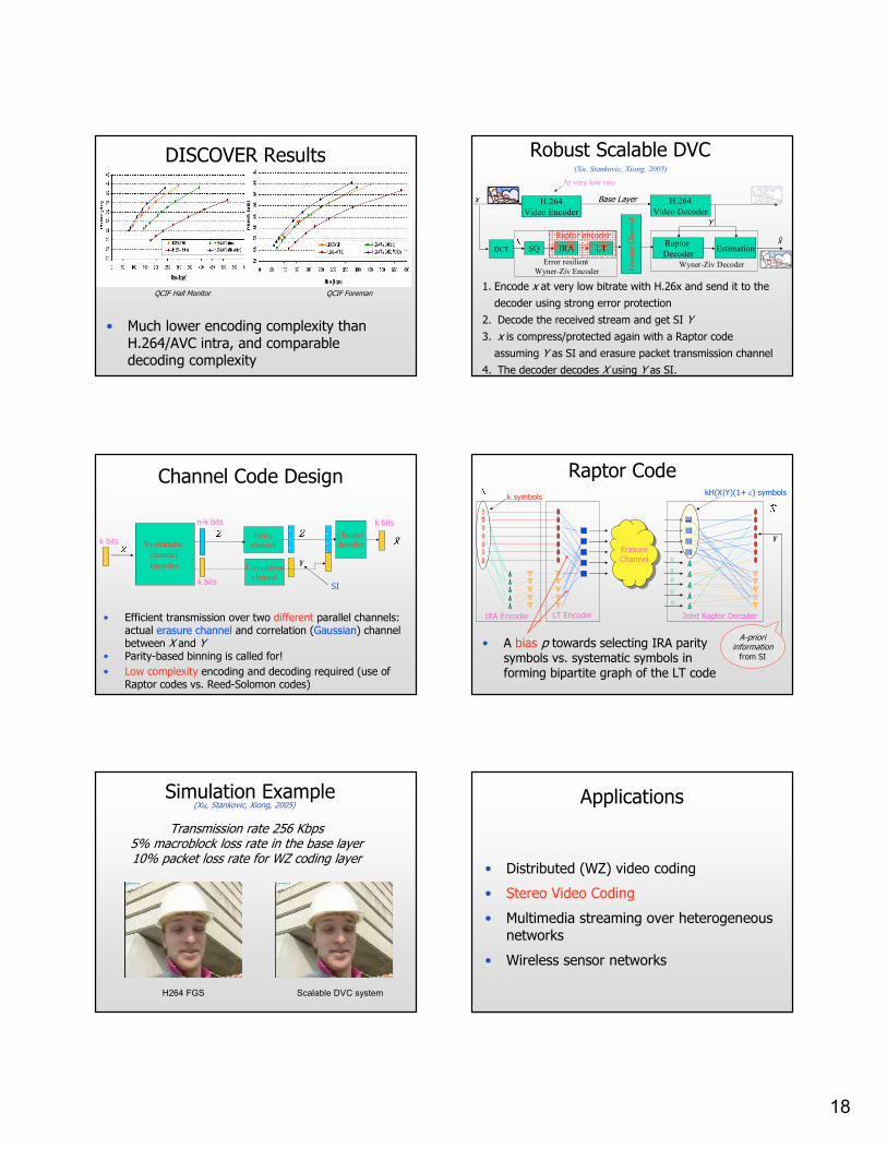
• Much lower encoding complexity than H.264/AVC intra, and comparable decoding complexity

DISCOVER Results Robust Scalable DVC

H.264

Video Encoder

H.264

Video Decoder

Era

sure

Chan

nel

DCT SQ IRARaptor

DecoderEstimation

Error resilient

Wyner-Ziv EncoderWyner-Ziv Decoder

x

x̂LT

Raptor encoder

Y

Base Layer

1. Encode x at very low bitrate with H.26x and send it to the

decoder using strong error protection

2. Decode the received stream and get SI Y

3. x is compress/protected again with a Raptor code

assuming Y as SI and erasure packet transmission channel

4. The decoder decodes X using Y as SI.

(Xu, Stankovic, Xiong, 2005)

At very low rate

Channel Code Design

Noisy

channel

Channel

decoder

Y

Systematic

channel

encoder

• Efficient transmission over two different parallel channels: actual erasure channel and correlation (Gaussian) channel between X and Y

• Parity-based binning is called for!

• Low complexity encoding and decoding required (use of Raptor codes vs. Reed-Solomon codes)

k bits

Correlation

channelk bits

k bits

SI

n-k bits

Raptor Code

Erasure Channel 0

0

0

0

0

IRA Encoder LT Encoder Joint Raptor Decoder

Y

AA--priori priori informationinformation

from SIfrom SI

k symbolskH(X|Y)(1+ ε) symbols

• A bias p towards selecting IRA parity symbols vs. systematic symbols in forming bipartite graph of the LT code

Scalable DVC systemH264 FGS

Transmission rate 256 Kbps5% macroblock loss rate in the base layer10% packet loss rate for WZ coding layer

Simulation Example(Xu, Stankovic, Xiong, 2005)

Applications





19

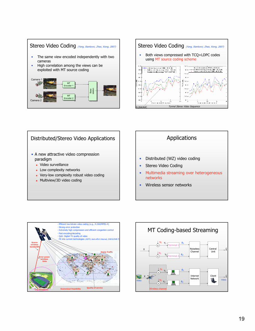
Stereo Video Coding (Yang, Stankovic, Zhao, Xiong, 2007)

• The same view encoded independently with two cameras

• High correlation among the views can be exploited with MT source coding

MT

Encoder 2

MT

Encoder 2

Ba

se

sta

tio

n

Ba

se

sta

tio

n

MT

Encoder 1

MT

Encoder 1

Camera 1

Camera 2

Stereo Video Coding (Yang, Stankovic, Zhao, Xiong, 2007)

• Both views compressed with TCQ+LDPC codes using MT source coding scheme

Tunnel Stereo Video SequenceH.264/AVC

Distributed/Stereo Video Applications

• A new attractive video compression paradigm

� Video surveillance

� Low complexity networks

� Very-low complexity robust video coding

� Multiview/3D video coding

Applications





Scarce wireless bandwidth

- Efficient low-bitrate video coding (e.g., H.264/MPEG-4)

Error-prone wireless links

- Strong error protection

Heavy Traffic

- Extremely high compression and efficient congestion control

Live Broadcast

- Fast encoding/decoding

Economical Feasibility

-Fit into current technologies (HDTV, best-effort Internet, DVB-S/DVB-T)

Quality of service

- QoS: Digital TV quality of video

MT Coding-based Streaming

X

+

+

N1

N2

Terminal 1

Terminal 2

Y1

Y2

NoiselessChannel

R1

R2

Central Unit

X^

X

+

+

N1

N2

Y1

Y2

InternetNetwork

R1

R2

Client X^

Video

Wireless channel

Video

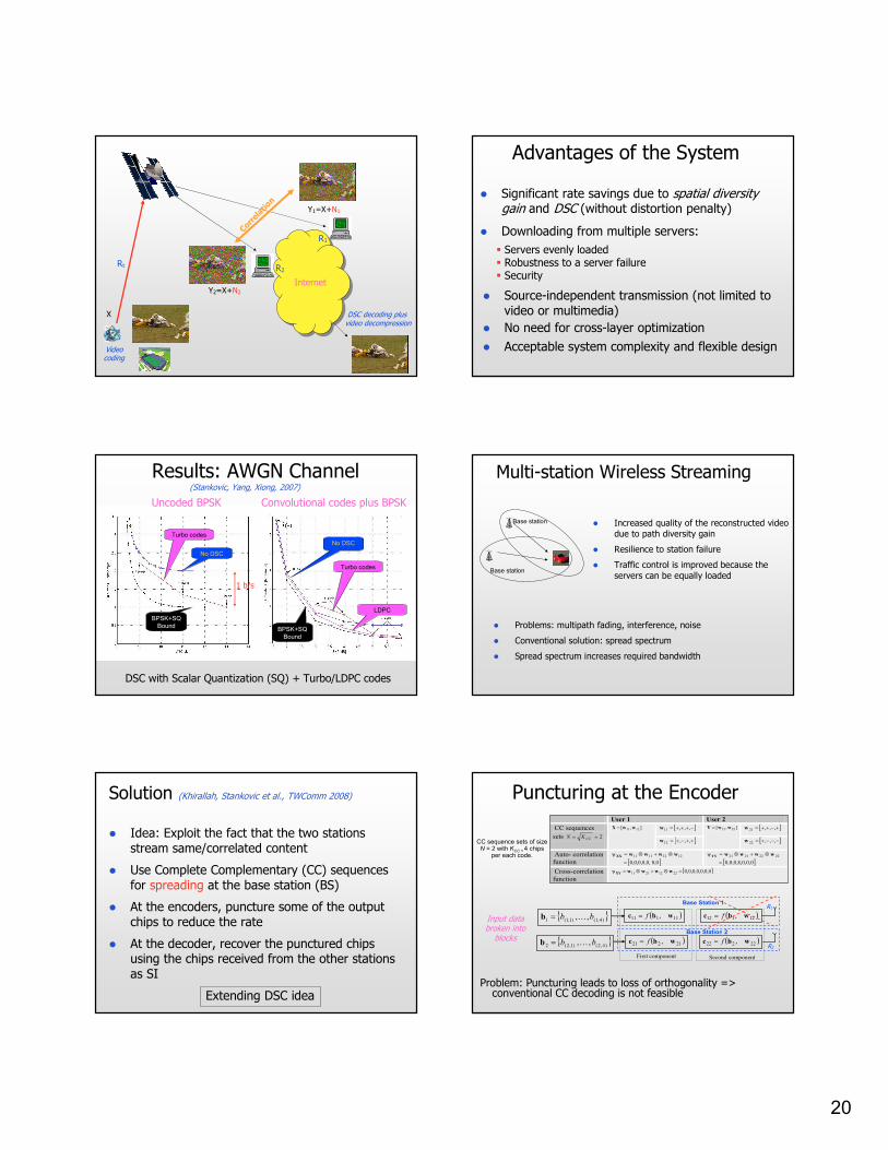
20

Video coding

Internet

DSC decoding plus video decompression

Y2=X+N2

Y1=X+N1

Rt R2

R1

X

Correlation

Advantages of the System

� Significant rate savings due to spatial diversity gain and DSC (without distortion penalty)

� Downloading from multiple servers:

� Source-independent transmission (not limited to video or multimedia)

� No need for cross-layer optimization

� Servers evenly loaded� Robustness to a server failure� Security

� Acceptable system complexity and flexible design

Results: AWGN Channel

DSC with Scalar Quantization (SQ) + Turbo/LDPC codes

BPSK+SQ

Bound

No DSC

Turbo codes

BPSK+SQ

Bound

No DSC

Turbo codes

LDPC

Uncoded BPSK Convolutional codes plus BPSK

1 b/s

(Stankovic, Yang, Xiong, 2007)

Multi-station Wireless Streaming

Base station

Base station� Increased quality of the reconstructed video

due to path diversity gain

� Resilience to station failure

� Traffic control is improved because the servers can be equally loaded

� Problems: multipath fading, interference, noise

� Conventional solution: spread spectrum

� Spread spectrum increases required bandwidth

Solution (Khirallah, Stankovic et al., TWComm 2008)

� Idea: Exploit the fact that the two stations stream same/correlated content

� Use Complete Complementary (CC) sequences for spreading at the base station (BS)

� At the encoders, puncture some of the output chips to reduce the rate

� At the decoder, recover the punctured chips using the chips received from the other stations as SI

Extending DSC idea

{ })4,1()1,1(1 ,, bb …=b

{ })4,2()1,2(2 ,, bb …=b

( )11111 , wbc f= ( )12112 , wbc f=

( )21221 , wbc f= ( )22222 , wbc f=

First component Second component

R1

R2

Base Station 1

Base Station 2

Puncturing at the Encoder

Problem: Puncturing leads to loss of orthogonality => conventional CC decoding is not feasible

Input data broken into

blocks

User 1 User 2

[ ]−+++= ,,,11w [ ]+−++= ,,,21w CC sequences

sets 2== CCKN

],[ 1211 wwX =

[ ]++−+= ,,,12w

],[ 2221 wwY =

[ ]−−−+= ,,,22w

Auto- correlation

function [ ]0,00,0,0,8,0,

ψ 12121111

=

⊗+⊗= wwwwXX [ ]0,0,0,8,0,0,0

ψ 22222121

=

⊗+⊗= wwwwYY

Cross-correlation

function

[ ]0,0,0,0,0,0,0ψ 22122111 =⊗+⊗= wwwwXY

CC sequence sets of size N = 2 with KCC = 4 chips

per each code.

21

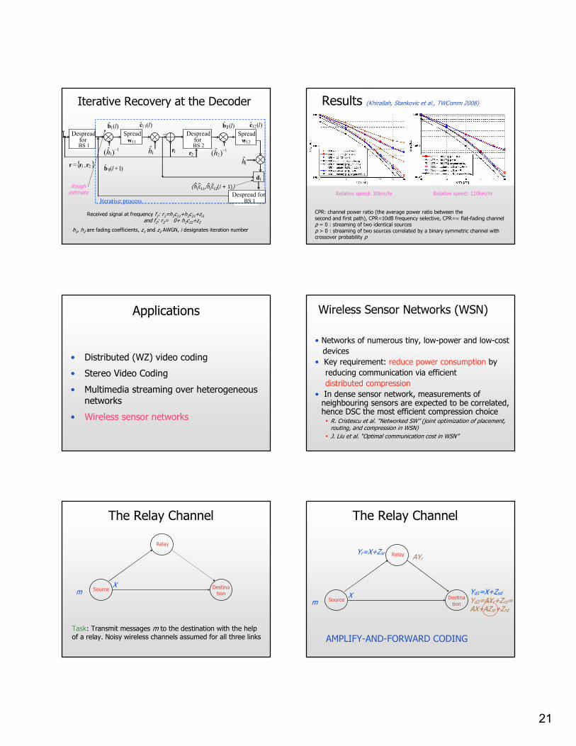
Iterative Recovery at the Decoder

Terminal 1

Terminal 1

Terminal 2

{ }21 ,rrr =

)(ˆ12 lc

Despreadfor BS 1

)(ˆ11 lc

Spread

11w

Despreadfor

Spread

12w

12)ˆ(

−h

11)ˆ(

−h 1r

_

1̂h

1d

Despread for

1̂h

)1(ˆ +l1b

Iterative process

)(ˆ1 lb )(ˆ l2b

2r

BS 2

BS 1

h1, h2 are fading coefficients, z1 and z2 AWGN, l designates iteration number

Received signal at frequency f1: r1=h1c11+h2c21+zi1

and f2: r2= 0+ h2c22+z2

{h1c11;h1c12(l + 1)}^^ ^^Rough estimate

Results (Khirallah, Stankovic et al., TWComm 2008)

Relative speed: 30km/hr Relative speed: 120km/hr

CPR: channel power ratio (the average power ratio between thesecond and first path), CPR=10dB frequency selective, CPR=∞ flat-fading channelp = 0 : streaming of two identical sourcesp > 0 : streaming of two sources correlated by a binary symmetric channel with crossover probability p

Applications





• Networks of numerous tiny, low-power and low-cost

devices

• Key requirement: reduce power consumption by

reducing communication via efficient

distributed compression

• In dense sensor network, measurements of neighbouring sensors are expected to be correlated, hence DSC the most efficient compression choice� R. Cristescu et al. “Networked SW” (joint optimization of placement,

routing, and compression in WSN)

� J. Liu et al. “Optimal communication cost in WSN”

Wireless Sensor Networks (WSN)

The Relay Channel

Source

Relay

Destinationm

X

Task: Transmit messages m to the destination with the help of a relay. Noisy wireless channels assumed for all three links

The Relay Channel

Source

Relay

Destinationm

X

Yr=X+Zsr

Yd1=X+Zsd

AYr

Yd2=AYr+Zrd=AX+AZsr+Zrd

AMPLIFY-AND-FORWARD CODING

22

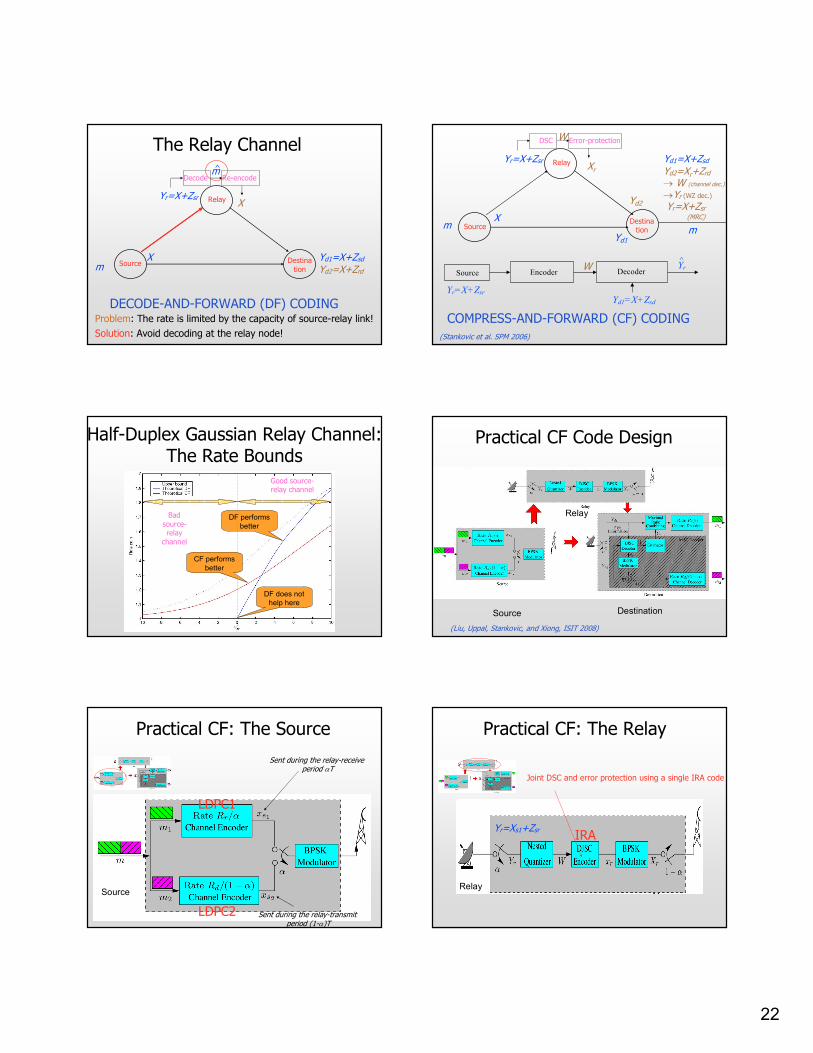
The Relay Channel

Source

Relay

Destinationm

X

Yr=X+Zsr

Yd1=X+Zsd

DECODE-AND-FORWARD (DF) CODINGProblem: The rate is limited by the capacity of source-relay link!

Yd2=X+Zrd

X

Decode Re-encodem^

Solution: Avoid decoding at the relay node!

Source

Relay

Destination

mX

Yr=X+Zsr Yd1=X+Zsd

COMPRESS-AND-FORWARD (CF) CODING

Yd2=Xr+Zrd

→ W (channel dec.)

→Yr (WZ dec.)

Yr=X+Zsr(MRC)

m

W

Xr

DSC Error-protection

EncoderSource

Yr=X+Zsr

WDecoder

^

Yd1=X+Zsd

Yr

Yd1

Yd2

(Stankovic et al. SPM 2006)

Half-Duplex Gaussian Relay Channel:The Rate Bounds

DF performs

better

DF does not

help here

CF performs

better

Bad source-relay

channel

Good source-relay channel

Practical CF Code Design

Source Destination

Relay

(Liu, Uppal, Stankovic, and Xiong, ISIT 2008)

Source

Practical CF: The Source

Sent during the relay-receive period αT

Sent during the relay-transmit period (1-α)T

LDPC1

LDPC2

Relay

Practical CF: The Relay

Joint DSC and error protection using a single IRA code

Yr=Xs1+ZsrIRA

23

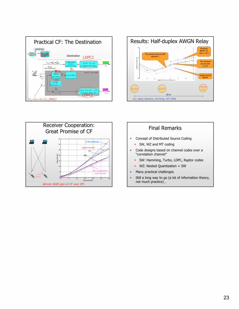
Destination

Practical CF: The Destination

=Xs1+Zsd

Yd2=Xs2+Xr+Zrd (MAC)

LDPC1

LDPC2

IRA

Results: Half-duplex AWGN Relay

Upper bound

BPSK

Practical

BPSK CF

with α=0.5

The scheme

bound with

α=0.5

The scheme bound with optimal α

Source RELAYDestina

tion

10 m

(Liu, Uppal, Stankovic, and Xiong, ISIT 2008)

Receiver Cooperation: Great Promise of CF

-10 0 10 20 30 40 500

5

10

15

20

25

30

35

Received SNR

Rate

(bit/s

/Hz)

2 Rx Antenna

Upper bound

CF

DF

No cooperation

upper/lower

Almost 20dB gain of CF over DF!

• Concept of Distributed Source Coding

� SW, WZ and MT coding

• Code designs based on channel codes over a “correlation channel”

� SW: Hamming, Turbo, LDPC, Raptor codes

� WZ: Nested Quantization + SW

• Many practical challenges

• Still a long way to go (a lot of information theory, not much practice)…

Final Remarks

Classic References:

Lossless Distributed Source Coding:

1. D. Slepian and J.K. Wolf, “Noiseless coding of correlated information sources,” IEEE Trans.

Inform. Theory, vol. IT-19, pp. 471-480, July 1973.

2. J.K. Wolf, “Data reduction for multiple correlated sources,” Proc. 5th Colloquium Microwave

Communication, pp. 287-295, June 1973.

3. A. Wyner, “Recent results in the Shannon theory,” IEEE Trans. Inform. Theory, vol. 20, pp. 2-

10, January 1974.

4. R.M. Gray and A.D. Wyner, “Source coding for a simple network,” Bell Syst. Tech. J., vol. 53,

pp. 1681-1721, November 1974.

5. T. Cover, “A proof of the data compression theorem of Slepian and Wolf for ergodic sources,”

IEEE Trans. Inform. Theory, vol. IT-21, pp. 226-228, March 1975.

6. A.D. Wyner, “On source coding with side information at the decoder,” IEEE Trans. Inform.

Theory, vol. IT-21, pp. 294-300, May 1975.

7. R.F. Ahlswede and J. Korner, “Source coding with side information and a converse for

degraded broadcast channels,” IEEE Trans. Inform. Theory, vol. IT-21, pp. 629-637, November

1975.

8. A. Sgarro, “Source coding with side information at several decoders,” IEEE Trans. Inform.

Theory, vol. IT-23, pp. 179-182, March 1977.

9. J. Korner and K. Marton, “Images of a set via two channels and their role in multi-user

communication,” IEEE Trans. Inform. Theory, vol. IT-23, pp. 751-761, November 1977.

10. S.I. Gel`fand and M.S. Pinsker, “Coding of sources on the basis of observations with

incomplete information,” Probl. Peredach. Inform., vol. 15, pp. 45-57, April-June 1979.

11. T.S. Han and K. Kobayashi, “A unified achievable rate region for a general class of

multiterminal source coding systems,” IEEE Trans. Inform. Theory, vol. IT-26, pp. 277-288, May

1980.

12. I. Csiszar and J. Korner, “Towards a general theory of source networks,” IEEE Trans. Inform.

Theory, vol. IT-26, pp. 155-165, March 1980.

13. T. S. Han, “Slepian-Wolf-Cover theorems for networks of channels,” Inform. and Control,

vol. 47, pp. 67.83, 1980.

14. I. Csiszar and J. Korner, Information Theory: Coding Theorems for Discrete Memoryless

Systems, Academic Press, 1981.

15. T. Cover and J. Thomas, Elements of Information Theory, New York: Wiley, 1991.

16. L. Song and R. W. Yeung, “Network information flow – multiple sources,” in Proc. ISIT-

2001 Int'l Symp. Inform. Theory, June 2001.

Lossy Distributed Source Coding:

1. A. Wyner and J. Ziv, “The rate-distortion function for source coding with side information at

the decoder,” IEEE Trans. Inform.Theory, vol. 22, pp. 1-10, January 1976.

2. T. Berger, “Multiterminal source coding”, The Inform. Theory Approach to Communications,

G. Longo, Ed., New York: Springer-Verlag, 1977.

3. S. Tung, Multiterminal Rate-distortion Theory, Ph. D. Dissertation, School of Electrical

Engineering, Cornell University, Ithaca, NY, 1978.

4. A. Wayner, “The rate-distortion function of source coding with side information at the

decoder-II: General sources,” Inform. Contr., vol. 38, pp. 60-80, 1978.

5. H. Yamamoto and K. Itoh, “Source coding theory for multiterminal communication systems

with a remote source,” Trans. IECE of Japan, vol. E63, pp. 700–706, October 1980.

6. A. Kaspi and T. Berger, “Rate-distortion for correlated sources with partially separated

encoders,” IEEE Trans. Inform. Theory, vol. 28, pp. 828-840, November 1982.

7. C. Heegard and T. Berger, “Rate-distortion when side information may be absent,” IEEE

Trans. Inform. Theory, vol. IT-31, pp. 727-734, November 1985.

8. T. Berger and R. Yeung, “Multiterminal source encoding with one distortion criterion,” IEEE

Trans. Inform. Theory, vol. 35, pp. 228-236, March 1989.

9. T. Flynn and R. Gray, “Encoding of correlated observations,” IEEE Trans. Inform. Theory, vol.

33, pp. 773–787, November 1987.

10. T. Berger, Z. Zhang, and H. Viswanathan, “The CEO problem,” IEEE Trans. Inform. Theory,

vol. 42, pp. 887-902, May 1996.

11. R. Zamir, “The rate loss in the Wyner-Ziv problem,” IEEE Trans. Inform. Theory, vol. 42, pp.

2073-2084, November 1996.

12. H. Viswanathan and T. Berger, “The quadratic Gaussian CEO problem,” IEEE Trans. Inform.

Theory, vol. 43, pp. 1549–1559, September 1997.

13. Y. Oohama, “Gaussian multiterminal source coding,” IEEE Trans. Inform. Theory, vol. 43,

pp. 1912-1923, November 1997.

14. Y. Oohama, “The rate-distortion function for the quadratic Gaussian CEO problem,” IEEE

Trans. Inform. Theory, vol. 44, pp. 1057–1070, May 1998.

15. R. Zamir and T. Berger, “Multiterminal source coding with high resolution,” IEEE Trans.

Inform. Theory, vol. 45, pp. 106–117, January 1999.

16. Y. Oohama, “Multiterminal source coding for correlated memoryless Gaussian sources with

several side information at the decoder,” Proc. ITW-1999 Information Theory Workshop, Kruger

National Park, South Africa, June 1999.

17. S. Servetto, “Lattice quantization with side information,” Proc. DCC-2000, Snowbird, UT,

March 2000.

18. R. Zamir, S. Shamai, and U. Erez, “Nested linear/lattice codes for structured multiterminal

binning”, IEEE Trans. Inform. Theory, vol. 48, pp. 1250–1276, June 2002.

19. S. Pradhan and K. Ramchandran, “Distributed source coding using syndromes (DISCUS):

Design and construction,” IEEE Trans. Inform. Theory, vol. 49, pp. 626–643, March 2003.

20. Y. Oohama, “Rate-distortion theory for Gaussian multiterminal source coding systems with

several side informations at the decoder,” IEEE Trans. Inform. Theory, vol. 38, pp. 2577-2593,

July 2005.

21. A. Wagner, S. Tavildar, and P. Viswanath, “The rate region of the quadratic Gaussian two-

encoder source-coding problem,” IEEE Trans. Inform. Theory, to appear.

Some Research Groups:

DSC Theory:

T. Cover, Stanford, http://www.stanford.edu/~cover/

Cornell University (T. Berger, A. Wagner, S. Wicker, L. Tong), http://www.ece.cornell.edu/

R. Zamir, Tel Aviv University, http://www.eng.tau.ac.il/~zamir/

Y. Oohama, University of Tokushima, http://pub2.db.tokushima-

u.ac.jp/ERD/person/147725/profile-en.html

M. Vetterli, EPFL, http://lcavwww.epfl.ch/~vetterli/

S. Pradhan, Mitchigen Ann Arbor, http://www.eecs.umich.edu/~pradhanv/

J. Chen, McMaster, http://www.ece.mcmaster.ca/~junchen/

DSC Code Design:

K. Ramchandran, Berkeley, http://basics.eecs.berkeley.edu/

Z. Xiong, TAMU, http://lena.tamu.edu/

F. Fekri, Georgia Tech, http://users.ece.gatech.edu/~fekri/

M. Effros, California Institute of Technology, http://www.ee2.caltech.edu/Faculty/effros/

J. Garcia-Frias, University of Delaware, http://www.ece.udel.edu/~jgarcia/ S. Pradhan, Mitchigen Ann Arbor, http://www.eecs.umich.edu/~pradhanv/

E. Magli, Politecnico di Torino, http://www.telematica.polito.it/sas-ipl/Magli/

IBM T. J. Watson Research Center, http://www.watson.ibm.com/

Mitsubishi Electric Research Labs, http://www.merl.com

DVC and other applications to multimedia:

B. Girod, Stanford, http://www.stanford.edu/~bgirod/

K. Ramchandran, Berkeley, http://basics.eecs.berkeley.edu/


DISCOVERY Project, http://www.discoverdvc.org/

A. Ortega, Southern California, http://sipi.usc.edu/~ortega/

E. Delp, Purdue, http://cobweb.ecn.purdue.edu/~ips/

E. Tuncel, University of California, River Side, http://www.ee.ucr.edu/~ertem/

A. Fernando, University of Surrey, http://www.ee.surrey.ac.uk/CCSR/research/ilab/

P. Frossard, http://lts4www.epfl.ch/~frossard/

P.L. Dragotti, Imperial College London, http://www.commsp.ee.ic.ac.uk/~pld/

Stankovic’s, University of Strathclyde, http://www.eee.strath.ac.uk/

Compress-and-forward:


E. Erkip, Polytechnic University, http://eeweb.poly.edu/~elza/

M. Gastpar, Berkeley, http://www.eecs.berkeley.edu/Faculty/Homepages/gastpar.html

J. Li (Tiffany), Lehigh University, http://www.cse.lehigh.edu/~jingli/

Motorola Labs Paris

Contact Details Distributed Source Coding: Theory and Practice · coding (NC) SW coding WZ coding...

Documents

Transcript of Contact Details Distributed Source Coding: Theory and Practice · coding (NC) SW coding WZ coding...