Consumption and the Great Recession;/media/publications/economic... · Federal Reserve Bank of...

1Federal Reserve Bank of Chicago

Introduction and summary

The Great Recession of 2008–09 was characterized by the most severe year-over-year decline in consumption the United States had experienced since 1945. The consumption slump was both deep and long lived. It took almost 12 quarters for total real personal con-sumption expenditures (PCE) to go back to its level at the previous peak (2007:Q4).

In this article, we document key facts about aggre-gate consumption and its subcomponents over time and look at the behavior of important determinants of consumption, such as consumers’ expectations about their future income and changes in consumers’ wealth positions related to house prices and stock valuations. Then, we use a simple permanent-income model to determine whether the observed drop in consumption can be explained by these observed drops in wealth and income expectations.

We begin our data analysis by using macroeco-nomic data to study the behavior of consumption and its subcomponents. We then use microeconomic data from the Reuters/University of Michigan Surveys of Consumers1 to study nominal expected income growth and inflationary expectations.

Our main findings from the macrodata are the fol-lowing. First, the Great Recession marked the most severe and persistent decline in aggregate consump-tion since World War II. All subcomponents of con-sumption declined during this period. However, the large drop in services consumption stands out most, relative to previous recessions. Second, while the de-cline was historic, the trends in consumption and its subcomponents leading up the recession were not substantially different from past recessionary periods. Third, the recovery path of consumption following the Great Recession has been uncharacteristically weak. It took nearly three years for total consumption to re-turn to its level just prior to the recession. In contrast,

the second-worst rebound observed in the data followed the 1974 recession and lasted just over one year. We find that this persistence is reflected most in the sub-components of nondurables and especially in services.

Our main findings from the analysis of the micro-data are as follows. First, expected nominal income growth declined significantly during the Great Recession. This is the worst drop ever observed in these data, and this measure has not yet fully recovered to pre-recession levels. Second, the decline exists for all age groups,

Consumption and the Great Recession

Mariacristina De Nardi, Eric French, and David Benson

Mariacristina De Nardi is a senior economist and research advisor; Eric French is a senior economist and research advisor; and David Benson is an associate economist in the Economic Research Department of the Federal Reserve Bank of Chicago. The authors thank Richard Porter and an anonymous referee for helpful comments and Helen Koshy for editorial advice.

© 2012 Federal Reserve Bank of Chicago Economic Perspectives is published by the Economic Research Department of the Federal Reserve Bank of Chicago. The views expressed are the authors’ and do not necessarily reflect the views of the Federal Reserve Bank of Chicago or the Federal Reserve System.Charles L. Evans, President ; Daniel G. Sullivan, Executive Vice President and Director of Research; Spencer Krane, Senior Vice President and Economic Advisor; David Marshall, Senior Vice President, financial markets group; Daniel Aaronson, Vice President, microeconomic policy research; Jonas D. M. Fisher, Vice President, macroeconomic policy research; Richard Heckinger,Vice President, markets team; Anna L. Paulson, Vice President, finance team; William A. Testa, Vice President, regional programs, Richard D. Porter, Vice President and Economics Editor; Helen Koshy and Han Y. Choi, Editors; Rita Molloy and Julia Baker, Production Editors; Sheila A. Mangler, Editorial Assistant.Economic Perspectives articles may be reproduced in whole or in part, provided the articles are not reproduced or distributed for commercial gain and provided the source is appropriately credited. Prior written permission must be obtained for any other reproduc-tion, distribution, republication, or creation of derivative works of Economic Perspectives articles. To request permission, please contact Helen Koshy, senior editor, at 312-322-5830 or email [email protected].

ISSN 0164-0682

2 1Q/2012, Economic Perspectives

FIguRE 2

Nominal PCE to nominal GDP ratio during recessions since 1962

PCE – GDP ratio

Notes: PCE is personal consumption expenditures; GDP is gross domestic product. Shaded areas indicate recession periods as defined by the National Bureau of Economic Research.

Source: Haver Analytics.

FIguRE 1

Level of real personal consumption expenditures

billions of 2005 dollars

Note: PCE is personal consumption expenditures.

Source: Haver Analytics.

1962 ’68 ’74 ’80 ’86 ’92 ’98 2004 ’100.54

0.56

0.58

0.60

0.62

0.64

0.66

0.68

0.70

0.72

education levels, and income quin-tiles. Relative to previous recessions, those with higher levels of income and education are more pessimistic coming out of this recession than their poorer and less-educated counterparts. Third, expectations for real income growth have also declined, and the decline in expected real income growth is more severe when personal inflation expectations are used instead of actual Consumer Price Index (CPI) inflation. Fourth, expected income growth is a strong predictor of actual future income growth. Since expected income growth is a very important determi-nant of consumption decisions, the observed drop in expected income has the potential to explain at least part of the observed decline in consumption.

In the context of a simple perma-nent-income model, we find that the negative wealth effect (coming from decreased stock market valuations and housing prices) and consumers’ decreased income expectations were big factors in determining the ob-served consumption drop. In fact, we find that in this model, the ob-served drops in wealth and income expectations can explain the observed drop in consumption in its entirety, depending on what we assume about future income growth beyond the time horizon covered by the Reuters/University of Michigan Surveys of Consumers data set.

Reinhart and Rogoff (2009) have stressed the similarities be-tween the current financial crisis and many earlier ones stretching across centuries, continents, and economies. These crises entailed large declines in real housing prices, equity collapses, and profound declines in out-put and employment. They emphasize the importance of balance sheet repair. We complement their research by emphasizing the role played by consumers’ income expectations, as well as wealth effects.

Macrodata: Total real PCE

Figure 1 displays the level of real PCE from 1962 to 2011:Q3. Even over this long horizon, the chart

shows a flattening out of the consumption growth rate in 2008–09. The fact that this pattern is clearly visible, even over a period of almost 50 years, highlights the severity and persistence of the Great Recession and the very slow recovery that is following it.

Figure 2 shows that consumption growth outpaced gross domestic product (GDP) growth through past recessionary periods. The nominal PCE–GDP ratio has increased in each recession since 1962. In contrast, during the Great Recession, it increased more modestly. Since the latest recession, this ratio has either fallen or stagnated. Thus, as a share of GDP, consumption

1962 ’70 ’78 ’86 ’94 2002 ’100

2,000

4,000

6,000

8,000

10,000


FIguRE 3

Normalized real PCE levels over recession periods

peak level = 1


Sources: Haver Analytics and authors’ calculations.

FIguRE 4

Real total quarterly PCE growth over 2008–09 versus previous recessions since 1974

quarterly growth (annual rate)



−16 −14 −12 −10 −8 −6 −4 −2 10 12 14 16

2007:Q4

2001:Q1

1990:Q3

1981:Q3

1980:Q1

1973:Q4

2 40 6 8

quarters since peak

0.80

0.85

0.90

0.95

1.00

1.05

1.10

1.15

1.20

−6

−4

−2

0

2

4

6

2007:Q4

Average of previous recessions

−16 −14 −12 −10 −8 −6 −4 −2 10 12 14 162 40 6 8

quarters since peak

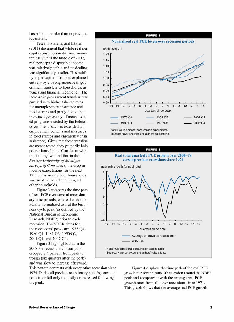
has been hit harder than in previous recessions.

Petev, Pistaferri, and Eksten (2011) document that while real per capita consumption declined mono-tonically until the middle of 2009, real per capita disposable income was relatively stable and its decline was significantly smaller. This stabil-ity in per capita income is explained entirely by a strong increase in gov-ernment transfers to households, as wages and financial income fell. The increase in government transfers was partly due to higher take-up rates for unemployment insurance and food stamps and partly due to the increased generosity of means-test-ed programs enacted by the federal government (such as extended un-employment benefits and increases in food stamps and emergency cash assistance). Given that these transfers are means tested, they primarily help poorer households. Consistent with this finding, we find that in the Reuters/University of Michigan Surveys of Consumers, the drop in income expectations for the next 12 months among poor households was smaller than that among all other households.

Figure 3 compares the time path of real PCE over several recession-ary time periods, where the level of PCE is normalized to 1 at the busi-ness cycle peak (as defined by the National Bureau of Economic Research, NBER) prior to each recession. The NBER dates for the recessions’ peaks are 1973:Q4, 1980:Q1, 1981:Q3, 1990:Q3, 2001:Q1, and 2007:Q4.

Figure 3 highlights that in the 2008–09 recession, consumption dropped 3.4 percent from peak to trough (six quarters after the peak) and was slow to increase afterward. This pattern contrasts with every other recession since 1974. During all previous recessionary periods, consump-tion either fell only modestly or increased following the peak.

Figure 4 displays the time path of the real PCE growth rate for the 2008–09 recession around the NBER peak and compares it with the average real PCE growth rates from all other recessions since 1971. This graph shows that the average real PCE growth


FIguRE 5

Normalized real PCE services over several recessions

peak level = 1

Notes: PCE is personal consumption expenditures. For each recession, the level of PCE services is normalized to 1 at the business cycle peak (as defined by the National Bureau of Economic Research) prior to the recession.


−16 −14 −12 −10 −8 −6 −4 −2 10 12 14 16

2007:Q4

2001:Q1

1990:Q3

1981:Q3

1980:Q1

1973:Q4

2 40 6 8

quarters since peak

0.80

0.85

0.90

0.95

1.00

1.05

1.10

1.15

1.20

FIguRE 6

Normalized real nondurables PCE over several recessions

peak level = 1

Notes: PCE is personal consumption expenditures. For each recession, the level of nondurables PCE is normalized to 1 at the business cycle peak (as defined by the National Bureau of Economic Research) prior to the recession.


−16 −14 −12 −10 −8 −6 −4 −2 10 12 14 16

2007:Q4

2001:Q1

1990:Q3

1981:Q3

1980:Q1

1973:Q4

2 40 6 8

quarters since peak

0.80

0.85

0.90

0.95

1.00

1.05

1.10

1.15

1.20

rate around the 2008–09 recession was significantly lower than the corresponding average over the previous five recessions. Consump-tion has grown 4.1 percent in total over the past five years, or an aver-age rate of 0.8 percent per year. This consumption growth rate con-trasts sharply with its average rate since 1971 of 3.1 percent, adding up to about 15 percent growth over an average five-year period. Thus, consumption expenditures are about 15% – 4% = 11% below what they would have been had they grown at their historical averages from 2007:Q4 onward.

All subcomponents of PCE fell during the Great Recession. Durables growth was somewhat weaker than in the previous five recessionary periods, both in terms of average growth rate and pattern of recovery. However, nondurables, and espe-cially services, were the most de-pressed compared with previous recessions.

Macrodata: Total real PCE services

Figure 5 highlights that the be-havior of PCE services was starkly different over the 2008–09 reces-sion from all other recessions since 1974. In all other recessions, PCE services grew both before and after the peak, while during the latest recession, it stagnated starting two quarters after the peak (four quar-ters before the trough) and kept stagnating for four additional quar-ters afterward. PCE services took until 2010:Q4 to return to peak levels.

Regarding the main services subcomponents, Petev, Pistaferri, and Eksten (2011) document that spending on health services in-creased, held stable for housing and utilities, but declined substantially for services related to transportation, food, and recreation. In sum, the most adjustable services dropped, while those components that the consumer has little discretion to adjust did not.

Macrodata: Total real nondurables PCE

We can see from figure 6 that the rise in PCE nondurables was similar to that experienced in most other recessions before the peak, but its recovery path


FIguRE 7

Normalized real durables PCE over several recessions

peak level = 1

Notes: PCE is personal consumption expenditures. For each recession, the level of durables PCE is normalized to 1 at the business cycle peak (as defined by the National Bureau of Economic Research) prior to the recession.


0.6

0.7

0.8

0.9

1.0

1.1

1.2

1.3

1.4

1.5

−16 −14 −12 −10 −8 −6 −4 −2 10 12 14 16

2007:Q4

2001:Q1

1990:Q3

1981:Q3

1980:Q1

1973:Q4

2 40 6 8quarters since peak

in the latest recession was among the worst.

Petev, Pistaferri, and Eksten (2011) document an unusual de-cline in spending on food, an im-portant indicator of consumer well-being, which raises concerns about the extent and depth of the strains on households during the latest recession. An interesting new paper by Aguiar, Hurst, and Karabarbounis (2011), however, documents that during the most re-cent recession, a significant fraction of foregone market work hours went to home production (based on diary information)—35 percent, including childcare. This is an im-portant channel that could produce more goods (such as food) and ser-vices (such as childcare) at a lower cost. More research is needed to determine if home production could completely explain the ob-served decline in food spending.

Macrodata: Total real PCE durables

Figure 7 displays a large drop for durables over the most recent recession. Five to six quarters after the peak, this recession actually displayed the largest drop in durables, compared with the previous five re-cessions. In addition, the pace of recovery in durables was slow—it took 12 quarters for durables to regain the previous peak level.

Petev, Pistaferri, and Eksten (2011) document that the bulk of the decline in real per capita spending is attributable to purchases of cars (a 25 percent decline by the end of 2008) and partly of furniture (a 9 percent decline).

To summarize, our main findings from the macro-data are as follows. First, the Great Recession marked the most severe and persistent decline in aggregate consumption since World War II. All subcomponents of consumption declined during this period. However, we find that the significant drop in consumed services stands out most, compared with previous recessions. Second, while the decline was historic, the time path of consumption and its subcomponents leading up the recession was not substantially different from past recessionary periods. Third, the recovery path of consumption following the Great Recession has been uncharacteristically weak. It took nearly three years for total consumption to return to its level just prior

to the recession. In contrast, the second-worst rebound observed in the data followed the 1974 recession and was just over one year. We find that this persistence is reflected most in the subcomponents of nondurables and especially in services consumption.

Microdata: Expected income

This section uses consumer expectations for future income from the Reuters/University of Michigan Surveys of Consumers, both in nominal and real terms, to see whether shocks to expected future income are contribut-ing to the consumption dip that we have experienced. The survey asks two questions to identify the magnitude and sign of income changes.

1. “During the next 12 months, do you expect your income to be higher or lower than during the past year?”

2. “By about what percent do you expect your income to (increase/decrease) during the next 12 months?”

The resulting index of expected income growth ranges widely across individuals, but on average, the estimates tend to accord with what we might have anticipated ex ante. The historical mean is +5.5 percent, split between +4.8 percent during recessions and +5.6 percent during expansions. While the realized


FIguRE 8

Realized and expected nominal disposable income

income growth

Sources: Haver Analytics, Reuters/University of Michigan Surveys of Consumers, and authors’ calculations.

FIguRE 9

Average expected nominal income growth rates around recessionary periods

expected nominal income growth

Sources: Reuters/University of Michigan Surveys of Consumers and authors’ calculations.

1978 ’82 ’86 ’90 ’94 ’98 2002 ’06 ’10−6

−4

−2

0

2

4

6

8

10

12

14

Nominal disposal income growth

Expected nominal income growth

−2

0

2

4

6

8

10

12

−16 −14 −12 −10 −8 −6 −4 −2 10 12 14 16

1980:Q1

1981:Q3

1990:Q3

2001:Q1

Great Recession 2007:Q4

2 40 6 8

quarters since peak

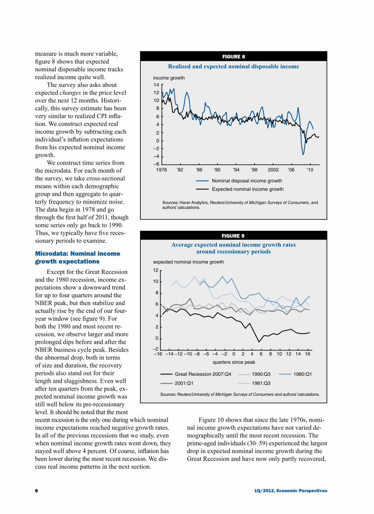
measure is much more variable, figure 8 shows that expected nominal disposable income tracks realized income quite well.

The survey also asks about expected changes in the price level over the next 12 months. Histori-cally, this survey estimate has been very similar to realized CPI infla-tion. We construct expected real income growth by subtracting each individual’s inflation expectations from his expected nominal income growth.

We construct time series from the microdata. For each month of the survey, we take cross-sectional means within each demographic group and then aggregate to quar-terly frequency to minimize noise. The data begin in 1978 and go through the first half of 2011, though some series only go back to 1990. Thus, we typically have five reces-sionary periods to examine.

Microdata: Nominal income growth expectations

Except for the Great Recession and the 1980 recession, income ex-pectations show a downward trend for up to four quarters around the NBER peak, but then stabilize and actually rise by the end of our four-year window (see figure 9). For both the 1980 and most recent re-cession, we observe larger and more prolonged dips before and after the NBER business cycle peak. Besides the abnormal drop, both in terms of size and duration, the recovery periods also stand out for their length and sluggishness. Even well after ten quarters from the peak, ex-pected nominal income growth was still well below its pre-recessionary level. It should be noted that the most recent recession is the only one during which nominal income expectations reached negative growth rates. In all of the previous recessions that we study, even when nominal income growth rates went down, they stayed well above 4 percent. Of course, inflation has been lower during the most recent recession. We dis-cuss real income patterns in the next section.

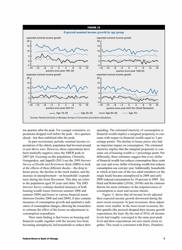
Figure 10 shows that since the late 1970s, nomi-nal income growth expectations have not varied de-mographically until the most recent recession. The prime-aged individuals (30–59) experienced the largest drop in expected nominal income growth during the Great Recession and have now only partly recovered,


FIguRE 10

Expected nominal income growth by age group




expected nominal income growth expected nominal income growth

quarters since peak 1981:Q3 quarters since peak 1990:Q3

quarters since peak 2001:Q1 quarters since peak 2007:Q4−Great Recession

Age 70+Age 60−69Age 30−59Age 18−29

−12 −8 −4 12 16−5

0

5

10

15

20

0 4 8−16

−12 −8 −4 12 16−5

0

5

10

15

20

0 4 8−16 −12 −8 −4 12 16−5

0

5

10

15

20

0 4 8−16

−12 −8 −4 12 16−5

0

5

10

15

20

0 4 8−16

ten quarters after the peak. For younger consumers, ex-pectations dropped well before the peak—five quarters ahead—but then stabilized after the peak.

In past recessionary periods, nominal income ex-pectations of the elderly population had hovered around or just above zero. However, these expectations have been markedly negative since the NBER peak in 2007:Q4. Focusing on this population, Christelis, Georgarakos, and Jappelli (2011) use the 2009 Internet Survey of Health and Retirement Study (HRS) to look at the effects of three different shocks—the drop in house prices, the decline in the stock market, and the increase in unemployment—on households’ expendi-tures during the Great Recession. This data set refers to the population aged 50 years and older. The HRS Internet Survey contains detailed measures of both housing wealth losses (between summer 2006 and summer 2009) and losses in various financial assets (between October 2008 and mid-2009). It also contains measures of consumption growth and qualitative indi-cators of consumption changes, allowing the researchers to estimate the effect of the losses on adjustments in consumption expenditure.

Their main finding is that losses on housing and financial wealth, together with the income loss from becoming unemployed, led households to reduce their

spending. The estimated elasticity of consumption to financial wealth implies a marginal propensity to con-sume with respect to financial wealth equal to 3 per-centage points. The decline in house prices also had an important impact on consumption: The estimated elasticity implies that the marginal propensity to con-sume out of housing wealth is 1 percentage point. Put differently, these estimates suggest that every dollar of financial wealth lost reduces consumption three cents per year and every dollar of housing wealth lost reduces consumption one cent per year. Additionally, households in which at least one of the two adult members (or the single head) became unemployed in 2008 and early 2009 reduced consumption by 10 percent in 2009. See Hurd and Rohwedder (2010a, 2010b) and the citations therein for more estimates on the responsiveness of consumption to asset and income shocks.

Figure 11 shows that all income levels adjusted their expected income growth downward during the most recent recession. In past recessions, these adjust-ments were smaller. In the most recent recession, the first quintile (the poorest) dropped their income growth expectations the least. By the end of 2010, all income levels had roughly converged to the same post-peak level and their expectations are now much closer to-gether. This result is consistent with Petev, Pistaferri,


FIguRE 11

Expected nominal income growth by income quintile





5th quintile4th quintile2nd quintile1st quintile



3rd quintile

−16 −12 −8 −4 12 16−5

0

5

10

15

0 4 8 −16 −12 −8 −4 12 16−5

0

5

10

15

0 4 8

−12 −8 −4 12 16−5

0

5

10

15

0 4 8−16 −12 −8 −4 12 16−5

0

5

10

15

0 4 8

and Eksten’s findings. First, they find that increased government transfers propped up income among the poorest households during the Great Recession. Second, using the Michigan Index of Consumer Sentiment (constructed using a subset of questions from the Reuters/University of Michigan Surveys of Consumers), they document that high-income individuals became more pessimistic than other groups during the Great Recession.2 Finally, using the Bureau of Labor Statistics’ Consumer Expenditure Survey (CEX), they find that respondents in the top decile of the wealth distribution are the ones who decreased spending during the Great Recession (–5.4 percent). This finding holds for the subcategories of nondurables and services. This drop in consumption might be due to the large negative wealth effect experienced by these households due to declining house prices and stock market valuations.

Figure 12 shows that in previous recessions, income expectations across education groups were rather flat over the cycle. In the most recent recession, everyone reduced their expected income growth.

Microdata: Real income growth expectations

Nominal income growth during the Great Recession was low, but realized inflation was also low. To study the behavior of real income expectations, we measure

inflation in two ways. First, we use actual CPI inflation over the 12-month period covered by the survey ques-tion, which assumes that consumers have perfect fore-sight over the next year concerning inflation. Second, we use the answer to the survey question about the individual’s expectation about growth in prices over the next 12 months. Using these two measures, we construct individual-level expected real income growth and then aggregate up to population-quarter means.

The two inflation series have diverged in the past, but after the late 1970s the differences are minor. At the start of the Great Recession, however, a large gap opened up, making for the largest discrepancy we have observed between these two data series. The swing in 2008:Q2 is +6 percent in expected inflation, compared with –1 percent actual CPI inflation. The two measures have since become much closer (see figure 13). The gap in these two measures, of course, affects measured real income growth expectations as we document next.

In figure 14, there is no clear cyclical pattern pri-or to the Great Recession in real income expectations. Before the most recent recession, real income growth was rather flat; it dropped into negative territory several quarters before the peak; and it then went up to about 4 percent four quarters after the peak. From then on, however, it had a large drop, reaching –3 percent five


FIguRE 12

Expected nominal income growth by educational level





FIguRE 13

Time series of 12 months forward inflation since 1978(CPI versus personal inflation expectations for the Reuters/University of Michigan Surveys of Consumers)

year-over-year inflation

Note: CPI is Consumer Price Index.


College +Some collegeHigh school graduatesHigh school dropouts



−12−15 −8 −4 12 160 4 8−5

0

5

10

15

−12−15 −8 −4 12 160 4 8−5

0

5

10

15

−12−15 −8 −4 12 160 4 8−5

0

5

10

15

−12−15 −8 −4 12 160 4 8−5

0

5

10

15

−6

−4

−2

0

2

4

6

8

10

12

14

16

1978 ’80 ’82 ’84 ’86 ’88 ’90 ’92 ’94 ’96 ’98 2000 ’02 ’04 ’06 ’08 ’10

CPI inflation

Consumer expected inflation


FIguRE 14

Expected real income growth, deflated by CPI inflation


Note: CPI is Consumer Price Index.


FIguRE 15

Expected real income growth, using consumers’ inflation expectations



−6

−4

−2

0

2

4

6

−16 −14 −12 −10 −8 −6 −4 −2 10 12 14 162 40 6 8

quarters since peak

1980:Q1

1981:Q3

1990:Q3

2001: Q1


−6

−4

−2

0

2

4

6

quarters since peak

1980:Q1

1981:Q3

1990:Q3

2001: Q1


−16 −14 −12 −10 −8 −6 −4 −2 10 12 14 162 40 6 8

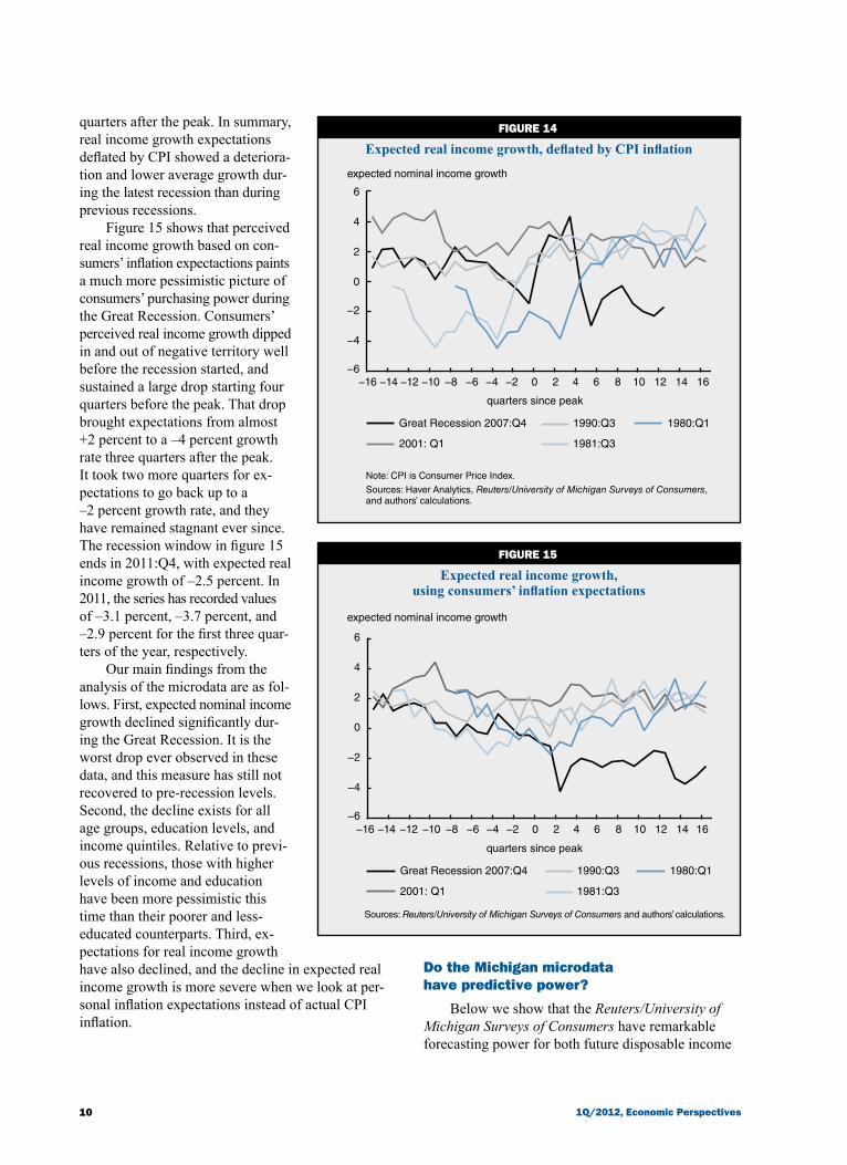
quarters after the peak. In summary, real income growth expectations deflated by CPI showed a deteriora-tion and lower average growth dur-ing the latest recession than during previous recessions.

Figure 15 shows that perceived real income growth based on con-sumers’ inflation expectactions paints a much more pessimistic picture of consumers’ purchasing power during the Great Recession. Consumers’ perceived real income growth dipped in and out of negative territory well before the recession started, and sustained a large drop starting four quarters before the peak. That drop brought expectations from almost +2 percent to a –4 percent growth rate three quarters after the peak. It took two more quarters for ex-pectations to go back up to a –2 percent growth rate, and they have remained stagnant ever since. The recession window in figure 15 ends in 2011:Q4, with expected real income growth of –2.5 percent. In 2011, the series has recorded values of –3.1 percent, –3.7 percent, and –2.9 percent for the first three quar-ters of the year, respectively.

Our main findings from the analysis of the microdata are as fol-lows. First, expected nominal income growth declined significantly dur-ing the Great Recession. It is the worst drop ever observed in these data, and this measure has still not recovered to pre-recession levels. Second, the decline exists for all age groups, education levels, and income quintiles. Relative to previ-ous recessions, those with higher levels of income and education have been more pessimistic this time than their poorer and less- educated counterparts. Third, ex-pectations for real income growth have also declined, and the decline in expected real income growth is more severe when we look at per-sonal inflation expectations instead of actual CPI inflation.

Do the Michigan microdata have predictive power?

Below we show that the Reuters/University of Michigan Surveys of Consumers have remarkable forecasting power for both future disposable income


and consumption growth.3 We estimate the regression for disposable income (Yt ) in period t first:

((Yt+k+4 – Yt+k )/Yt+k ) = α0 + α1 ((Yt – Yt–4)/Yt–4) + α2 gMt + εt+k ,

where α0, α1, α2 are parameters to be estimated, and α1 and α2 are reported in table 1. The variable ((Yt+k+4 – Yt+k )/Yt+k ) is next year’s annual income growth k quarters from now, so k is 0 when forecasting income growth over the next year and 4 when fore-casting income growth over the subsequent year. ((Yt – Yt–4 )/Yt–4 ) is income growth over the past year, and gMt is expected real income growth from the Michigan surveys, where we deflate using expected inflation from the survey.

As can be seen in table 1, lagged income growth has a negative coefficient, and expected income growth has a positive coefficient. The coefficient on expected income growth in the next year is 0.8, indicating that a 1 percent decline in expected income growth reduces next year’s income growth 0.8 percent, taking into account the previous year’s income growth. The right-hand column shows that predicted income growth over

the next year (2011:Q3 to 2012:Q3), using lagged income growth and expected income growth, is 0.6 per-cent, well below its average of 2.8 percent over the 1978–2011 sample period. Income growth between 2012:Q3 and 2013:Q3 is also forecasted to be low.

Expected income growth also turns out to be a good predictor of consumption growth. Table 1 presents regressions using future consumption growth as the left-hand-side variable and lagged consumption growth and the Michigan expectations variable as the right-hand-side variables. Using these estimates, the con-sumption forecast for 2011:Q3 to 2012:Q3 calls for a meager growth rate of 0.1 percent.

In short, the low expected income growth in the expectations data of the Reuters/University of Michigan Surveys of Consumers suggests that the U.S. will ex-perience low growth in both income and consumption over the next two years. Obviously, there are many things not included in this specification, so the estimates should only be taken as suggestive. However, the results are fairly robust to changes in model specification and to the addition of a few other variables, such as the unemployment rate.

TaBlE 1

Regression results

Lagged Lagged Forecasted income Michigan consumption annual growth income growth growth,Dependent variable variable expectations variable Q3/Q3 R-squared

Annual income growth –0.35 0.80 — 0.61* 0.29 1 year forward (0.10) (0.17)

Annual income growth 0.06 0.36 — 1.24** 0.08 2 years forward (0.08) (0.17)

Annual income growth –0.34 0.42 — 2.16*** 0.08 3 years forward (0.13) (0.20)

Annual consumption growth — 0.71 0.08 0.05* 0.37 1 year forward (0.23) (0.13)

Annual consumption growth — 0.77 –0.25 0.13** 0.18 2 years forward (0.23) (0.16)

Annual consumption growth — 0.58 –0.49 1.15*** 0.11 3 years forward (0.27) (0.19)

Annual consumption growth –0.20 0.75 0.18 0.39* 0.39 1 year forward (0.14) (0.21) (0.14)

Annual consumption growth 0.10 0.76 –0.31 –0.07** 0.17 2 years forward (0.14) (0.23) (0.19)

Annual consumption growth –0.09 0.59 –0.44 1.36*** 0.11 3 years forward (0.16) (0.27) (0.21)

Notes: Regressions are run with data from 1978:Q1 to 2011:Q2. Newey-West standard errors in parentheses. Average annual income and consumption growth are 2.78 and 2.91, respectively. Using data up to 2011:Q3, forecast of growth between: *2011:Q3 and 2012:Q3; **2012:Q3 and 2013:Q3; ***2013:Q3 and 2014:Q3.

Sources: Authors’ calculations based on data from Haver Analytics and Reuters/University of Michigan Surveys of Consumers.


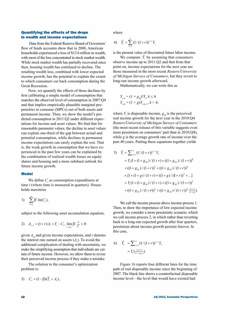
Quantifying the effects of the drops in wealth and income expectations

Data from the Federal Reserve Board of Governors’ flow of funds accounts show that in 2008, American households experienced a loss of $13.6 trillion in wealth, with most of the loss concentrated in stock market wealth. While stock market wealth has partially recovered since then, housing wealth has continued to decline. The resulting wealth loss, combined with lower expected income growth, has the potential to explain the extent to which consumers cut back consumption during the Great Recession.

Now, we quantify the effects of these declines by first calibrating a simple model of consumption that matches the observed level of consumption in 2007:Q4 and that implies empirically plausible marginal pro-pensities to consume (MPCs) out of both assets and permanent income. Then, we show the model’s pre-dicted consumption in 2011:Q2 under different expec-tations for income and asset values. We find that for reasonable parameter values, the decline in asset values can explain one-third of the gap between actual and potential consumption, while declines in permanent income expectations can easily explain the rest. That is, the weak growth in consumption that we have ex-perienced in the past few years can be explained by the combination of realized wealth losses on equity shares and housing and a more subdued outlook for future income growth.

Model

We define Ct as consumption expenditures at time t (where time is measured in quarters). House-holds maximize

10

) ln( ),t t

ttC

=

∞

∑β

subject to the following asset accumulation equation,

2 1 01) ( ) , limA r A Y Ct t t tt

t AC

t

t

+→∞

= + + − =β

given At 0 and given income expectations, and r denotes the interest rate earned on assets (At ). To avoid the additional complication of dealing with uncertainty, we make the simplifying assumption that individuals are cer-tain of future income. However, we allow them to revise their perceived income process if they make a mistake.

The solution to the consumer’s optimization problem is:

3 1) ( )( )C Y At t t= − +β � ,

where 4 1 1) ( ( ))Y r Yt

t

t= / +=

∞−∑

τ

ττ

is the present value of discounted future labor income.

We compute Yt by assuming that consumers observe income up to 2011:Q2 and that from that point on, income expectations for the next year are those measured in the most recent Reuters/University of Michigan Surveys of Consumers, but they revert to long-run income growth afterward.

Mathematically, we can write this as

Yt+k = (1 + gM )kYt, k ≤ 4

Yt+k = (1 + g)Yt+k−1, k > 4,

where Yt is disposable income, gM is the perceived real income growth for the next year in the 2010:Q4 Reuters/University of Michigan Surveys of Consumers (the most recent release of this variable suggests even more pessimism on consumers’ part than in 2010:Q4), while g is the average growth rate of income over the past 40 years. Putting these equations together yields

5 1 1

1 1 1 1 1

) ( ( ))

( ( ) ( ) (( ) ( ))

Y r Y

Y g r g r

t tt

t M M

= / +

= + + / + + + / +

=

∞ −∑ττ

τ

22

3 41 1 1 1

1 1 1 1

+ + / + + + / +

× + + / + + + /

(( ) ( )) (( ) ( ))

[ ( ) ( ) (( ) (

g r g r

g r gM M

11

1 1 1 1 1

1 1

2

2

+ + ...

= + + / + + + / +

+ + / +

r

Y g r g r

g

t M M

M

)) ]

( ( ) ( ) (( ) ( ))

(( ) ( rr g rMr

r g)) (( ) ( )) )( )( )

3 4 11 1+ + / + .+−

We call the income process above income process 1. Then, to show the importance of low expected income growth, we consider a more pessimistic scenario, which we call income process 2, in which rather than reverting back to a long-run expected growth after four quarters, pessimism about income growth persists forever. In this case,

6 1 11

) ( ( ))

( )( )( )

Y r Y

Y

t tt

tr

r gM

= / +

= .

=

∞ −

+−

∑ττ

τ

Figure 16 reports four different lines for the time path of real disposable income since the beginning of 2007. The black line shows a counterfactual disposable income level—the level that would have existed had


it continued to grow at its historical average rate of 3.2 percent from 2007:Q4 onward. The blue line shows realized disposable income up to 2011:Q2. The grey dotted line begins with realized disposable income in 2011:Q2. It then tacks on the expected level of disposable income using expectations data from the Reuters/University of Michigan Surveys of Consumers for all periods thereafter. This corresponds to income process 2. The blue dotted line begins in 2012:Q2, assuming that income grows according to the Reuters/University of Michigan Surveys of Consumers between 2011:Q2 and 2012:Q4 and then at its historical rate afterwards. It corresponds to income process 1.

CalibrationThe three key moments we wish to match are the

marginal propensity to consume (MPC) out of assets, the MPC out of permanent income, and the level of consumption in 2007:Q4.

Most estimates of the MPC out of assets are in the range 0.01–0.05, and most estimates of the MPC out of permanent income are between 0.5 and 1. We assume the MPC out of assets is 0.03 per year. We use per capita income growth for the individual’s de-cision problem. Thus, we set g = .032 – .014 = .018 (average disposable income growth over the 1967:Q4 to 2007:Q4 period less population growth of those

aged 16 and older over the same period). We then pick r and β to match the MPC out of assets and the level of consumption in 2007:Q4. Thus, we match

∂CAt

t∂= − = .( )1 03β

C Y rr g

A

Q Q

Q

2007 4 2007 4

2007 4

1 1: :

:

= −+−

+

( )[

],

β

where C2007:Q4 = $9,312.6 billion (at an annualized rate), Y2007:Q4 = $9,944 billion (annualized), and A2007:Q4 = $69,139 billion.

The unit of time in this analysis is a quarter. So, we convert annual growth rates to quarterly ones, using the formula (1 + g)(1/4) – 1 when taking the quarterly growth rate for g. For dollar amounts, we divide by 4. After converting everything to quarterly rates, we use the above two equations to solve for β and r. Table 2 presents all variables at quarterly and annualized rates. At annualized rates, β = 0.97 and r = 0.060.This gives a quarterly MPC out of permanent income equal to

∂∂

= − + / − = .CY

r r gt

t

( )[( ) ( )] ,1 1 730β

FIguRE 16

Disposable income and assumed income processes



2006 ’07 ’08 ’09 ’10 ’11 ’129,500

10,000

10,500

11,000

11,500

12,000

Disposable income Counterfactual disposable income

Income process 1 Income process 2


TaBlE 2

Model parameters

Annual Quarterly (dollars in billions)

Exogenously set gM – 0.016 – 0.0040Population growth 0.014 0.0035g 0.018 0.0045MPC out of assets 0.030 0.0074 Y2007:Q4 9,944 2,486C2007:Q4 9,313 2,328A2007:Q4 69,139 69,139

Endogenously determinedβ 0.970 0.993r 0.060 0.015Implied MPC out of income 0.730

Note: MPC is marginal propensity to consume.

Sources: Authors’ calculations based on data from Haver Analytics and the Reuters/University of Michigan Surveys of Consumers.

2007:Q4 and predict Y as of 2011:Q2, had income grown steadily at its long-run historical average. Second, we calculate Y , given realized income in 2007:Q4 and the two income processes that we described previously. To be clear, taking into account population growth rates, we calculate Y Q2011 2: ,� given the information set from 2007:Q4, as 11 14gr

r g ,+−

�Y =2011:Q2 2007:Q4 1 pY ) ( ++(( ))where the term in the exponent (14) is the number of quarters between 2007:Q4 and 2011:Q2.

Once we calculate the loss in Y under different income and interest rate scenarios, we use the model to calculate the resulting consumption loss. The con-sumption loss associated with income process 1 is $0.917 trillion, which is reasonably close to the ob-served consumption loss. This computation is sensitive to the time path of the interest rate as well. The baseline calibration yields a yearly interest rate of 6 percent. In the lower short-term interest rate scenario, we assume that over the first year the yearly interest rate is 3 percent and then reverts back to 6 percent. In this case, income is less heavily discounted; hence its present value is higher and the implied consumption drop is smaller, $710 billion rather than $917 billion. Unsurprisingly, the very pessimistic income expectation scenario con-sidered in income process 2 generates a huge consump-tion loss of $4.038 trillion, which is almost four times larger than the consumption shortfall we wish to explain.

TaBlE 3

Results

Realized consumption level 2011:Q2 9,379Predicted consumption level 2011:Q2, given information in 2007:Q4 10,472Consumption loss 1,093

Consumption loss due to asset value decline Asset value decline 9,746Predicted consumption decline due to asset price decline 289

Consumption loss, given disposable income decline Income process 1 917Income process 1 and lower short-term interest rate 710Income process 2 4,038

Consumption loss given both asset and income declines Income process 1 1,206Income process 1 and lower short-term interest rate 999Income process 2 4,328

Note: All amounts in billions of dollars.

Sources: Authors’ calculations and data from Haver Analytics.which is about in the middle of the normal range esti-mates in the literature for the MPC.

Over the past 40 years, annual population growth for those aged 16 and older is 1.4 percent, which we define as p. We assume this rate of population growth continues in the future. Income growth in the individ-ual’s decision problem is in per capita terms. We then account for aggregate growth at the end by adjusting up disposable income by 1.4 percent at an annual rate.

Results

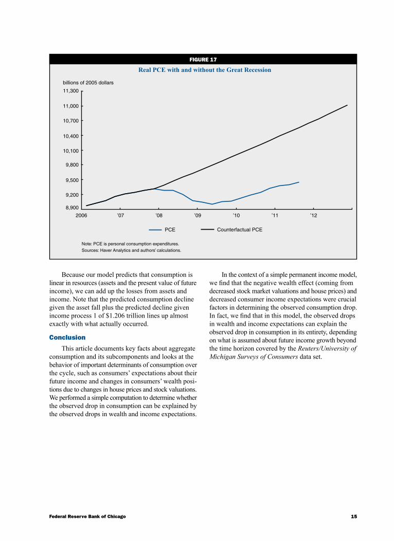
Table 3 explains our key findings. All quarterly numbers in this section are annualized; that is, they are the quarterly flows multiplied by 4. Consumption ex-penditures in 2011:Q2 were $9,379 billion. Had they grown at average rates from 2007:Q4 onward, they would have been at $10,472 billion in 2011:Q2, which is 10 percent higher than they are today. This difference of $1,093 billion, line 3 of the table, is the shortfall we seek to explain with the model. Figure 17 depicts this shortfall graphically.

Lines 4 and 5 in table 3 trace out the effects of the decline in asset prices. Net worth fell $9,746 billion in real terms over this period. Given a quarterly MPC of 0.0074 out of assets, we predict a ($9,746 billion) × (0.0074) × 4 = $289 billion fall in consumption, at an annualized rate.

The following lines in the table predict the consump-tion fall due to various permanent income scenarios. To perform this computation, we first put ourselves in


Because our model predicts that consumption is linear in resources (assets and the present value of future income), we can add up the losses from assets and income. Note that the predicted consumption decline given the asset fall plus the predicted decline given income process 1 of $1.206 trillion lines up almost exactly with what actually occurred.

Conclusion

This article documents key facts about aggregate consumption and its subcomponents and looks at the behavior of important determinants of consumption over the cycle, such as consumers’ expectations about their future income and changes in consumers’ wealth posi-tions due to changes in house prices and stock valuations. We performed a simple computation to determine whether the observed drop in consumption can be explained by the observed drops in wealth and income expectations.

In the context of a simple permanent income model, we find that the negative wealth effect (coming from decreased stock market valuations and house prices) and decreased consumer income expectations were crucial factors in determining the observed consumption drop. In fact, we find that in this model, the observed drops in wealth and income expectations can explain the observed drop in consumption in its entirety, depending on what is assumed about future income growth beyond the time horizon covered by the Reuters/University of Michigan Surveys of Consumers data set.

FIguRE 17

Real PCE with and without the Great Recession




2006

8,900

9,200

9,500

9,800

10,100

10,400

10,700

11,000

11,300

PCE Counterfactual PCE

’07 ’08 ’09 ’10 ’11 ’12


1This survey also collects the data that form the well-known Michigan Consumer Confidence Index. The survey is published monthly by the University of Michigan and Thomson Reuters.

2As a possible explanation for the pessimism of the wealthy, Shapiro (2010) finds that these households were exposed more to the stock market and experienced larger declines in wealth as a

consequence. The median decline in wealth was 15% in Shapiro’s data, and those who lost at least 10% of their net worth had almost twice the mean wealth and 3.5 times the median wealth of the sample.

3See Souleles (2004), Ludvigson (2004), and Barsky and Sims (2009) for more on the predictive power of the Michigan surveys.

Aguiar, Mark A., Erik Hurst, and Loukas Karabarbounis, 2011, “Time use during recessions,” National Bureau of Economic Research, working paper, No. 17259, July.

Barsky, Robert B., and Eric R. Sims, 2009 “Infor-mation, animal spirits, and the meaning of innova-tions in consumer confidence,” National Bureau of Economic Research, working paper, No. 15049, June.

Christelis, Dimitris, Dimitris Georgarakos, and Tullio Jappelli, 2011 “Wealth shocks, unemployment shocks and consumption in the wake of the Great Recession,” University of Naples, Italy, Centre for Studies in Economics and Finance, working paper, No. 279, October.

Hurd, Michael D., and Susann Rohwedder, 2010a, “Effects of the financial crisis and Great Recession on American households,” National Bureau of Economic Research, working paper, No. 16407, September.

__________, 2010b, “The effects of the economic crisis on the older population,” University of Michigan, Michigan Retirement Research Center, working paper, No. WP 2010-231, March.

Ludvigson, Sydney C., 2004, “Consumer confidence and consumer spending,” Journal of Economic Perspectives, Vol. 18, No. 2, Spring, pp. 29–50.

Petev, Ivaylo, Luigi Pistaferri, and Itay Saporta Eksten, 2011, “Consumption and the Great Recession: An analysis of trends, perceptions, and distributional effects,” Stanford University, mimeo, August.

Reinhart, Carmen M., and Kenneth S. Rogoff, 2009, This Time Is Different: Eight Centuries of Financial Folly, Princeton, NJ: Princeton University Press.

Shapiro, Matthew D., 2010, “The effects of the financial crisis on the well-being of older Americans: Evidence from the cognitive economic study,” University of Michigan, Michigan Retirement Research Center, working paper, No. WP 2010-228, September.

Souleles, Nicholas S., 2004, “Expectations, heteroge-neous forecast errors, and consumption: Micro evidence from the Michigan Consumer Sentiment Surveys,” Journal of Money, Credit and Banking, Vol. 36, No. 1, February.

NOTES

REFERENCES

Consumption and the Great Recession;/media/publications/economic... · Federal Reserve Bank of...

Documents

Transcript of Consumption and the Great Recession;/media/publications/economic... · Federal Reserve Bank of...