NBER WORKING PAPER SERIES

CONSUMER SPENDING AND THE ECONOMIC STIMULUS PAYMENTS OF2008

Jonathan A. ParkerNicholas S. Souleles

David S. JohnsonRobert McClelland

Working Paper 16684http://www.nber.org/papers/w16684

NATIONAL BUREAU OF ECONOMIC RESEARCH1050 Massachusetts Avenue

Cambridge, MA 02138January 2011

We thank Jeffrey Campbell, Adair Morse, Joel Slemrod, and participants at the 2009 ASSA meeting,the Fall 2010 NBER Economic Fluctuations and Growth Research Meeting, and seminars at the Boardof Governors of the Federal Reserve System, the Federal Reserve Bank of Chicago, Kellogg, Michigan,Princeton, Wisconsin and Wharton for helpful comments. We thank the staff of the Division of ConsumerExpenditure Surveys at the Bureau of Labor Statistics for their work in getting the economic stimuluspayment questions added to the Consumer Expenditure Survey. Parker thanks the Zell Center at theKellogg School of Management for funding. The views expressed in this paper are those of the authorsand do not necessarily correspond to those of the U.S. Census Bureau, the Bureau of Labor Statistics,or the National Bureau of Economic Research.

© 2011 by Jonathan A. Parker, Nicholas S. Souleles, David S. Johnson, and Robert McClelland. Allrights reserved. Short sections of text, not to exceed two paragraphs, may be quoted without explicitpermission provided that full credit, including © notice, is given to the source.

Consumer Spending and the Economic Stimulus Payments of 2008Jonathan A. Parker, Nicholas S. Souleles, David S. Johnson, and Robert McClellandNBER Working Paper No. 16684January 2011JEL No. D12,D14,D91,E21,E62,E65,H24,H31

ABSTRACT

We measure the response of household spending to the economic stimulus payments (ESPs) disbursedin mid-2008, using special questions added to the Consumer Expenditure Survey and variation arisingfrom the randomized timing of when the payments were disbursed. We find that, on average, householdsspent about 12-30% (depending on the specification) of their stimulus payments on non-durable expendituresduring the three-month period in which the payments were received. Further, there was also a significantincrease in spending on durable goods, in particular vehicles, bringing the average total spending responseto about 50-90% of the payments. Relative to research on the 2001 tax rebates, these spending responsesare estimated with greater precision using the randomized timing variation. The estimated responsesare substantial and significant for older, lower-income, and home-owning households. We furtherextend the literature in two ways. First, we find little evidence that the propensity to spend varies withthe method of disbursement (paper check versus electronic transfer). Second, we evaluate a complementarymethodology for quantifying the impact of tax cuts, which asks consumers to self-report whether theyspent their tax cuts. The response of spending to the ESPs is indeed largest for self-reported spenders.However, self-reported savers also spent a significant fraction of the payments.

Jonathan A. ParkerFinance DepartmentKellogg School of ManagementNorthwestern University2001 Sheridan RoadEvanston, IL 60208-2001and NBERJonathan-Parker@Kellogg.Northwestern.edu

Nicholas S. SoulelesFinance DepartmentThe Wharton School2300 SH-DHUniversity of PennsylvaniaPhiladelphia, PA 19104-6367and NBERsouleles@wharton.upenn.edu

David S. JohnsonUS Census BureauRoom 7H174Washington, DC 20233-8500david.s.johnson@census.gov

Robert McClellandSuite 31052 Massachusetts Ave NEWashington DC 20212-0001McClelland.Robert@bls.gov

1

In the winter of 2007-08, facing the fallout from an increasingly severe financial crisis

and already contemplating the limitations of traditional monetary policy, Congress and the

Administration turned to fiscal policy to help stabilize the U.S. economy. The Economic

Stimulus Act (ESA) of 2008, enacted in February 2008, consisted primarily of a 100 billion

dollar program that sent economic stimulus payments (ESPs) to approximately 130 million U.S.

tax filers. The desirability of this historically-important use of fiscal policy depends critically on

the extent to which these tax cuts directly changed household spending, as well as on any

subsequent multiplier or price effects.

In this paper, we measure the direct spending effect caused by the receipt of the ESPs, the

existence of which is a necessary (though not sufficient) condition for the efficacy of this

counter-cyclical policy. We begin by measuring the average spending response of households,

using variation in the randomized timing of when the ESPs were disbursed. Further, to help

improve our understanding of consumption in this recession and our models of consumer

behavior in general, we also analyze the heterogeneity in the spending response across

households with different characteristics and across different categories of consumption

expenditures. Finally, we evaluate whether another well-known and complementary

methodological approach to identifying the impact of tax cuts -- asking consumers to self-report

whether they spent (or intend to spend) their tax cuts (e.g., Shapiro and Slemrod, 2009) --

accurately identifies households that do and do not actually spend their tax cuts.

We measure the spending effects of the 2008 ESPs using a natural experiment provided

by the structure of the payments. The ESPs varied across households in amount, method of

disbursement, and timing. Typically, single individuals received $300-$600 and couples received

$600-$1200; in addition, households received $300 per child that qualified for the child tax

credit. Households received these payments through either paper checks sent by mail or

electronic funds transfers (EFTs) into their bank accounts. Most importantly, within each

disbursement method, the timing of receipt was determined by the final two digits of the

recipient’s Social Security number (SSN), digits that are effectively randomly assigned.1 We

exploit this random variation to cleanly estimate the causal effect of the payments on household 1 The last four digits of an SSN are assigned sequentially to applicants within geographic areas (which determine the first three digits of the SSN) and a “group” (the middle two digits of the SSN).

2

spending, by comparing the spending of households that received payments in a given period to

the spending of households that received payments in other periods.

To conduct our analysis, we worked with the staff at the Bureau of Labor Statistics (BLS)

to add supplemental questions about the payments to the ongoing Consumer Expenditure (CE)

Survey, which contains comprehensive measures of household-level expenditures for a stratified

random sample of U.S. households. These supplemental questions ask CE households to report

the amount and month of receipt of each stimulus payment they received, as well as the method

of disbursement of each payment (mailed paper check versus EFT). The responses to these

questions allow us to measure the impact of the payments on the spending of CE households and

study the extent to which the method of disbursement influences the propensity to spend. We

also added a question asking households who previously received stimulus payments to self-

report whether they thought their payments were mostly spent, mostly saved, or mostly used to

pay down debt. This question mimics the questions in the Michigan Survey of Consumers that

have been used to study recent changes in tax policy, as in Shapiro and Slemrod (2003a).

Summarizing our main findings, on average households spent about 12-30% of their

stimulus payments, depending on the specification, on non-durable consumption goods and

services (as defined in the CE survey) during the three-month period in which the payments were

received. This response is statistically and economically significant. Although our findings do

not depend on any particular theoretical model, the response is inconsistent with both Ricardian

equivalence, which implies no spending response, and with the canonical life-cycle/permanent

income hypothesis (LCPIH), which implies that households should consume at most the

annuitized value of a transitory increase in income like that induced by the one-time stimulus

payments. We also find a significant effect on the purchase of durable goods and related

services, primarily the purchase of vehicles, bringing the average response of total consumption

expenditures to about 50-90% of the payments during the three-month period of receipt.

These results are statistically and economically broadly consistent across specifications

that use different forms of variation, including specifications that focus on the randomized timing

variation within each of the two disbursement methods. The estimated spending responses are

statistically and economically similar for ESPs received by EFT compared to those received by

mail, although there is little temporal variation in the former group with which to identify the key

effect. We also find some evidence of an ongoing though smaller response in the subsequent

3

three-month period following that of ESP receipt, but this response cannot be estimated with

precision.

The point estimates of the fraction of the ESPs spent suggest that, relative to the effects

of the 2001 tax rebates estimated in Johnson, Parker, and Souleles (2006) (JPS), in 2008 the

spending effect was slightly smaller for nondurable expenditures but more targeted towards

durables. While this finding may be due to sampling error, it may also reflect some of the

differences in the details of the tax cut and economic environment in 2008 compared to earlier

periods. For instance, on average the stimulus payments in 2008 were about twice the size of the

rebates in 2001, consistent with some prior research that finds that larger payments lead to a

different composition of spending. While JPS finds no significant response of durable goods in

2001, Souleles (1999) finds a significant increase in both nondurable and durable goods (in

particular auto purchases) in response to spring-time Federal income tax refunds, which are

substantially larger than the 2001 tax rebates.2

Our results suggest a significant macroeconomic effect of the 2008 ESPs. The point

estimates imply that the ESPs directly caused an increase in consumer demand for CE-defined

nondurable expenditures of $32 to $80 billion (at an annual rate) in the second quarter of 2008

and $15 to $36 billion (at an annual rate) in the third quarter. Our estimates for total CE

spending imply a direct increase of about 1.3 to 2.3 percent of personal consumption

expenditures (PCE) in the second quarter, and 0.6 to 1.0 percent of PCE in the third quarter

(again at annual rates).3 We return to these numbers in the conclusion, but here note again that

these direct effects on nominal spending demand may have also led to higher prices (not only

increases in real spending) and/or additional spending through multiplier effects.

As for results that further inform theories of consumer behavior and credit markets,

across households, the responses are largest for older and low-income households, groups which

have substantial and statistically significant spending responses. According to the point

estimates, the responses are largest for high-asset households, but this result is not statistically

2 See also Barrow and McGranahan (2000) and Adams, Einav, and Levin (2009) for related results for the EITC and for subprime auto sales. Federal tax refunds currently average around $2500 per recipient, whereas the average rebate in 2001 came to about $480 (JPS). 3 These figures are based on estimates in Tables 4 and 5 and so omit statistically-insignificant lagged spending. The calculations assume that the contemporaneous estimates represent spending done in the month of receipt and the month after. Using estimates from Table 7 that include lagged spending effects, the corresponding estimates are, for CE-defined nondurable expenditures, $66 billion in the second quarter and $75 billion in the third, and for total spending, $198 billion in the second quarter and $227 billion in the third, or 1.9 and 2.2 percent of PCE respectively.

4

significantly different from zero. Further, motivated by the collapse of the housing market in

2008, we find that homeowners on average spent more of their ESPs than did renters, a

difference that is statistically significant at the ten percent level.

Finally, turning to the evaluation of self-reports, we find that households that self-report

that they mostly spent their ESPs on average did spend more than self-reported savers, yet the

self-reported savers (including those reporting they reduced debt) also spent a statistically and

economically significant fraction of their payments. This suggests that relying on self-reports can

understate the actual causal change in spending in response to changes in income like tax cuts.

In addition to analyzing the amount of spending directly caused by the 2008 ESPs, our

paper builds on the related literature in a number of ways. First, relative to JPS, as discussed

below, we measure with greater precision the response of spending when focusing on random

variation in the timing of ESP receipt. Second, we consider whether the disbursement method

(check versus EFT) affects the amount of spending. The 2008 tax cut was the first large tax cut

to use EFTs, and EFTs seem likely to be used increasingly frequently in the future. Third, we

evaluate the accuracy of the self-reported responses to the payments, by comparing the self-

reports to our causal estimates using the data on actual spending and ESP receipt. Such an

evaluation is useful given the potential benefits of surveys that elicit such self-reported data. E.g.,

such surveys can be put into the field and analyzed quickly after policy changes, and they can be

used to evaluate hypothetical policies and the relevance of different theoretical reasons for

households’ reported behavior. As a result, the results from such surveys are widely reported.

This paper is structured as follows. Sections I and II briefly describe the literature and

relevant aspects of ESA 2008. Section III describes the CE data and Section IV sets forth our

empirical methodology. Section V presents the main results regarding the short-run response to

the economic stimulus payments, while Section VI examines the longer-run response. Sections

VII and VIII examine the differences in response across different households, and across

different categories of expenditure, respectively. After a concluding section, the Appendices

contain additional information about ESA 2008 and the data.

I. Related Literature

Of the many papers that test the consumption-smoothing implications of the rational-

expectations LCPIH, the most closely related to our work is the set of papers that uses

5

household-level data and quasi-experiments to identify the effects on consumption caused by

predictable changes in income, including in particular income changes induced by tax policy.

Deaton (1992), Browning and Lusardi (1996), JPS, and Jappelli and Pistaferri (2010) review

these literatures well.4

Our paper is most closely related to JPS, which uses a similar module of questions

appended to the CE survey to study the 2001 income tax rebates. JPS finds a relatively large

response in nondurable expenditure, amounting to about 20-40% of the rebates on average

during the three-month period in which they were received, but no significant response in

durable goods. Unlike the current study, however, JPS is unable to identify the response of

nondurables with precision using only the random variation in timing of rebate receipt. JPS finds

larger than average responses for households with low liquid wealth or low income, and a

significant though decaying lagged spending effect, so that on average roughly two-thirds of the

rebates was spent cumulatively during the quarter of receipt and subsequent three-month period.5

Agarwal, Liu, and Souleles (2007) finds consistent results using credit card data and

direct indicators of being credit constrained; in particular, the spending responses are largest for

consumers that are constrained by their credit limits. Shapiro and Slemrod (2003a) finds, using

the Michigan Survey of Consumers, that about 22% of respondents who received (or expected to

receive) a 2001 rebate report that they will mostly spend their rebate. The authors calculate that,

under certain assumptions, this result implies an average marginal propensity to consume (MPC)

of about one third, which is consistent with the short-run response of expenditure in JPS

estimated from data on actual spending and rebate receipt.

A few other studies also investigate the 2008 ESPs. First, using scanner data on a subset

of nondurable retail goods in the first few weeks after the payments started to be disbursed,

Broda and Parker (2008) finds that spending on such goods increased by a significant amount,

3.5% in the four weeks after payment receipt. The increase is larger than average for low asset

and low income households. Second, using data from a payday lender, Bertrand and Morse

(2009) finds that receipt of an ESP initially reduces the probability of taking out a payday loan.

The magnitude of the reduction in debt is modest relative to the ESPs, and, after two cycles,

4 For a survey of recent fiscal policy, see e.g., Auerbach and Gale (2009). 5 Johnson, Parker, and Souleles (2009) finds qualitatively similar responses to the 2003 child tax credit payments using CE data. Coronado, Lupton, and Sheiner (2006) also study the 2003 child payments, using the Michigan Survey.

6

borrowing returns to its pre-ESP level on average. For the most constrained borrowers, by

contrast, debt does not decline, consistent with the spending dynamics discussed in Agarwal,

Liu, and Souleles (2007).

Third, Shapiro and Slemrod (2009) uses the Michigan Survey to analyze the 2008

stimulus payments, and finds similar results as in Shapiro and Slemrod (2003a), with about 20%

of respondents self-reporting that they will mostly spend their payment. This again corresponds

to an average MPC of about one third. This response is larger than expected under the LCPIH for

a transitory tax cut, and it implies a noticeable expansionary effect on aggregate consumption in

the second and third quarters of 2008. The Michigan survey results provide no clear evidence of

greater spending by low-income or potentially constrained households.6

Finally, Bureau of Labor Statistics (2009) reports various summary statistics about the

CE data on the ESPs and self-reported usage. Nearly half of CE households reported that they

used their ESP mostly to pay down debt, 18% reported they mostly saved their ESP, and 30%

reported that they mostly spent it, more than found in Shapiro and Slemrod (2009).

II. The 2008 Economic Stimulus Payments

ESA 2008 provided ESPs to the majority of U.S. households (roughly 85% of “tax

units”). The ESP consisted of a basic payment and -- conditional on eligibility for the basic

payment -- a supplemental payment of $300 per child that qualified for the child tax credit. To be

eligible for the basic payment, a household needed to have positive net income tax liability, or at

least sufficient “qualifying income”.7 For eligible households, the basic payment was generally

the maximum of $300 ($600 for couples filing jointly) and their tax liability up to $600 ($1,200

6 In 2008, of the 80 percent of respondents who report they will mostly save their ESP, the majority (about 60 percent) report that they will mostly pay down debt (as opposed to accumulate assets). See also Sahm, Shapiro and Slemrod (2010). The Michigan Survey includes additional subjective questions about expected future spending. Of respondents who said they will initially mostly use the rebate to pay down debt, most report that they will “try to keep [down their] lower debt for at least a year.” (There are analogous results for respondents who said they will save by accumulating assets.) The Survey included similar questions in 2001 and yielded similar results (Shapiro and Slemrod, 2003b). By contrast, using data on actual spending in 2001, Agarwal, Liu, and Souleles (2007) finds that, while on average households initially used some of their rebates to increase credit card payments and thereby pay down debt, the resulting liquidity was soon followed by a substantial increase in spending. 7 While the stimulus payments were commonly referred to as “tax rebates,” strictly speaking they were advance payments for credit against tax year 2008 taxes. To expedite the disbursement of the payments, they were calculated using data from the tax year 2007 returns (and so only those filing 2007 returns received the payments). If subsequently a household’s tax year 2008 data implied a larger payment, the household could claim the difference on its 2008 return filed in 2009. However, if the 2008 data implied a smaller payment, the household did not have to return the difference.

7

for couples). Households without tax liability received basic payments of $300 ($600 for

couples), so long as they had at least $3,000 of qualifying income (which includes earned income

and Social Security benefits, as well as certain Railroad Retirement and veterans’ benefits).

Moreover, the total stimulus payment phased out with income, being reduced by five percent of

the amount by which adjusted gross income exceeded $75,000 ($150,000 for couples). As a

result, the stimulus payments were more targeted to lower-income households than were the

2001 income tax rebates.

The key to our measurement strategy is that the timing of ESP disbursement was

effectively randomized across households. Table 1 shows the schedule of ESP disbursement.8

For recipients who had provided the IRS with their personal bank routing number (i.e., for direct

deposit of a tax refund), the stimulus payments were disbursed electronically over a three-week

period ranging from late April to mid May.9 The IRS mailed a notice to the recipients in advance

of the EFTs. Appendix A provides an example of this notice. For households that did not provide

a personal bank routing number, the payments were mailed using paper checks over a nine-week

period ranging from early May through early July.10 The recipients of these checks received a

similar notice in advance of the checks.11 Importantly, within each disbursement method, the

particular timing of the payment was determined by the last two digits of the recipients’ Social

Security numbers, which are effectively randomly assigned.

8 The IRS schedule reports the latest date by which the ESPs are supposed to have been received by households. Accordingly, as also discussed below, the payments were disbursed (ie, put in the mail or electronically transferred to banks) slightly earlier. 9 Payments were directly deposited only to personal bank accounts. Payments were mailed to tax filers who had provided the IRS with their tax preparer’s routing number, eg as part of taking out a “refund anticipation loan”. Such situations are common, representing about a third of the tax refunds delivered via direct deposit in 2007. 10 Due to the electronic deposits, about half of the aggregate stimulus payments were disbursed by the end of May. While most of the rest of the payments came in June and July, taxpayers that filed their 2007 return late could receive their payment later than the above schedule. Since about 92 percent of taxpayers typically file at or before the normal April 15th deadline (Slemrod et al., 1997), this source of variation is small. Nonetheless, we present results below that exclude such late payments. Finally, due to human and computer error, about 350,000 households (less than 1 percent) did not receive the child tax credit component of their ESP with their basic ESP. The IRS took steps to identify these households and sent all affected households paper checks for the amount due for just the child credit, starting in early July. 11 For paper checks, the notices were mailed about a week before the checks were mailed. For EFTs, the notices were sent a couple of business days before the direct deposits were supposed to be credited. The recipients’ banks were also notified a couple of days before the date of the electronic transfers, and some banks might have credited some of the electronic payments to the recipients’ accounts a day or more before the official payment date. For example, some EFTs deposited on Monday April 28 were reported to the banks on Thursday April 24, and some banks appear to have credited accounts on Friday April 25.

8

In aggregate the stimulus payments in 2008 were historically large, amounting to about

$100 billion, which in real terms is about double the size of the 2001 rebate program. According

to the Department of the Treasury (2008), $78.8 billion in ESPs was disbursed in the second

quarter of 2008, which corresponds to about 2.2% of GDP or 3.1% of PCE in that quarter.

During the third quarter, $15 billion in ESPs was disbursed, corresponding to about 0.4% of

GDP or 0.6% of PCE. The stimulus payments constituted about two-thirds of the total ESA

package, which also included various business incentives and foreclosure relief.12 This paper

focuses on the stimulus payments, as recorded in our CE dataset.

III. The Consumer Expenditure Survey

The CE interview survey contains detailed measures of the expenditures of a stratified

random sample of U.S. households. CE households are interviewed five times. After an

introductory interview that collects demographic and income information, households are

interviewed up to four more times, at three month intervals. In these second to fifth interviews,

households report their expenditures during the preceding three months (the “reference period”).

The CE survey also gathers some limited information about wealth. New households are added

to the survey every month, so the data can be used to identify spending effects from ESPs

disbursed in different months. We use the 2007 and 2008 waves of the CE data (which include

interviews in the first quarter of 2009).

Two special modules of questions about the 2008 ESPs were added to the CE survey in

interviews conducted between June 2008 and March 2009, which covers the crucial time during

which the payments were disbursed.13 The first module of questions was phrased to be consistent

with the style of other CE questions and the 2001 tax rebate questions. The new questions asked

households whether they received any “economic stimulus payments… also called a tax rebate”

since the beginning of the reference period for the interview and, if so, the amount of each

payment and the date it was received. Going beyond the 2001 questions, this first module also

asked, for each payment, whether it was received by check or direct deposit. These questions

were asked in all five CE interviews.14

12 For more details on ESA, see e.g., CCH (2008) and Sahm, Shapiro and Slemrod (2010). 13 Ideally, since some ESPs arrived in April, the survey would have been in the field in May, e.g. for respondents whose last interview was in May. 14 In the introductory interview, the ESP reference period is the preceding one month.

9

The second module, also new in 2008, was asked at most once, and only of households

that had previously reported a payment. These households were asked whether the payment led

them “mostly to increase spending, mostly to increase savings, or mostly to pay off debt.” The

wording of this question closely follows the main question in the Michigan Survey of Consumers

analyzed by Shapiro and Slemrod (2009). Appendix B contains the language of the CE survey

instruments.

Turning to our use of the CE data, for each household-reference period, we follow JPS

and sum all stimulus payments received by the household in that three-month period to create

our main economic stimulus payment variable, ESP. We also follow JPS in our definition of

expenditures. Specifically, we focus on a series of increasingly aggregated measures of

consumption expenditures. First, we study expenditures on food, which include food consumed

away from home, food consumed at home, and purchases of alcoholic beverages. Much previous

research has studied such expenditure on food, largely because of its availability in most years of

the Panel Study of Income Dynamics, but it is a narrow measure of expenditure. Our second

measure of consumption expenditures is a subset of nondurable expenditures, denoted “strictly

nondurable” expenditures, which follows Lusardi (1996) and includes CE categories like

utilities, household operations, gas, personal care, and tobacco. Third, our broadest and main

measure of spending on nondurable goods and services, denoted nondurable expenditures,

follows previous research using the CE survey and includes semi-durable categories like apparel,

health and reading materials. Finally, total expenditures also includes durable expenditures such

as home furnishings, entertainment equipment, and auto purchases.15 Appendix C provides

further details about the data.

For our analysis, we use only data on households that have at least one expenditure

interview during the period in which the ESP questions were in the field. The resulting sample

period starts with interviews in September 2007 (when period t in equation (1) below covers

expenditures in June to August 2007) and runs through interviews in March 2009 (when period

t+1 covers December 2008 to February 2009). Also, we drop from the sample any household

15 Unlike in JPS, we find that the spending effect on total expenditures in 2008 is estimated with relative statistical precision. This could in part reflect the larger number of payments (about 30 percent more) in the sample in 2008, and the larger size (over double) of these payments. Suggestive of an improvement in data quality, there is also a decline in the ratio of the standard deviation of the change in household-level expenditures to the average level of expenditures between 2001 and 2008 for all our major categories. This may be due to the CE survey’s transition in 2003 from using survey booklets to using computer-assisted personal-interview (CAPI) software.

10

observation (t or t+1) with implausibly low expenditures (the bottom 1% of nondurable

expenditures in levels), unusually large changes in age or family size, and uncertain stimulus

payment status.16

Figure 1 shows our calculations of the aggregate amount of ESPs reported in the raw CE

data by month, and the corresponding amount of ESP disbursement reported in the Daily

Treasury Statements (DTS) (Department of the Treasury (2008)). During 2008, the ESPs

reported in the CE survey aggregate to $94.6 billion, which is quite close to the $96.2 billion in

ESPs in the DTS data. The temporal pattern of ESP receipt is also broadly similar across the two

sources, though the CE data has fewer ESPs reported during the peak month of May and more in

the following months. This suggests the possibility that some households took time to notice

their ESP receipt, or that there is some other tendency to report a somewhat later date of receipt

than actually occurred.

Table 2 presents summary statistics for our final full sample and subsamples that we

further analyze. The average value of ESP, conditional on a positive value, is about $1000.

Households that receive ESPs by EFT have slightly higher expenditures, are slightly younger,

have higher incomes and liquid assets, and have larger ESPs, than households that receive the

payments by mail.

Table 3 shows more information about the distribution of ESPs in our dataset. Panel A

shows that, consistent with the payments specified by ESA, most reported ESPs are in multiples

of $300, with about 55% of reports reflecting the (maximum) basic payments of $600 or $1,200.

Panel B shows the pattern of ESPs by interview reference period. During the expenditure

reference period that covers the main time of disbursement of the payments (May - July), about

two-thirds of households report receiving a payment.

IV. Empirical Methodology

Consistent with specifications in the previous literature (e.g., Zeldes (1989), Lusardi

(1996), Parker (1999), Souleles (1999), and JPS), our main estimating equation is:

Ci,t+1 - Ci,t = !s "0s*months,i + "1'Xi,t + "2 ESPi,t+1 + ui,t+1 , (1)

16 Our initial analysis of the ESP data uncovered a peculiar pattern in the raw data. When we notified the BLS, they determined that there had been an internal processing error, and worked rapidly to release a corrected version of the ESP data. We use this corrected version.

11

where i indexes households and t indexes time, C is either household consumption expenditures

or their log; month represents a complete set of indicator variables for every period in the

sample, used to absorb the seasonal variation in consumption expenditures as well as the average

of all other concurrent aggregate factors; and X represents control variables (here age and

changes in family size) included to absorb some of the preference-driven differences in the

growth rate of consumption expenditures across households. ESPi,t+1 represents our key stimulus

payment variable, which takes one of three forms: i) the total dollar amount of payments

received by household i in period t+1 (ESPi,t+1); ii) a dummy variable indicating whether any

payment was received in t+1 (I(ESPi,t+1>0)); and iii) a distributed lag of ESP or I(ESP >0), used

to measure the longer-run effects of the payments. We correct the standard errors to allow for

arbitrary heteroskedasticity and within-household serial correlation. As an extension, to analyze

heterogeneity in the response to the payments, we interact ESPi,t+1 with indicators for different

types of households. The key coefficient "2 measures the average response of household

expenditure to the arrival of a stimulus payment.17

Most of the recent literature on the LCPIH focuses on testing the null hypothesis that "2

is zero using variation in predictable changes in income and the assumption that the residual

(ui,t+1) is orthogonal to all information potentially known to a household at the start of period t,

including the change in income (Chamberlain, 1984; Souleles, 2004). By contrast, we can use

the randomized timing of ESP receipt to ensure orthogonality between the residual and the

predictable change in income that comes with the arrival of an ESP. This allows us to estimate "2

and thus measure the causal effect of the payments on expenditure, regardless of whether the

LCPIH is true or not. That said, our estimate still provides a direct test of the LCPIH.18 The

rational-expectations LCPIH (or Ricardian equivalence) implies that "2=0. Even if instead

17 Our empirical approach focuses on consumers’ response to the receipt of their stimulus payments, a point in time that our data identifies. Our methodology cannot estimate the magnitude of any earlier response that may have occurred in anticipation of the payments, both because the passage of ESA cannot be separated from other aggregate effects captured by our time dummies, such as seasonality, and because there is no single point in time at which a tax cut went from being entirely unexpected to being entirely expected. 18 Even though February 2008 can fall in period t for some sample households receiving a payment, under our maintained assumptions, any effect of the announcement on spending due to the passage of ESA does not bias our estimate of "2. Whenever information about the tax cuts underlying the ESPs became publicly available, whether preceding the actual passage of ESA or not, any resulting wealth effects should be small, and should have arisen at the same time(s) for all consumers, so their average effects on expenditure would be picked up by the corresponding time dummies in equation (1). More importantly, heterogeneity in such wealth effects (or in !2) should not be correlated with the timing of ESP receipt, so (the average) "2 should still be estimated consistently.

12

households were actually surprised by the payment, "2 should still be small under the LCPIH,

because the one-time payment represents a transitory increase in income.

V. The Short-Run Response of Expenditure

This section estimates the short-run change in consumption expenditures caused by

receipt of the stimulus payments, using the contemporaneous payment variables ESPt+1 and

I(ESPt+1>0) in equation (1). We begin by estimating (the average) "2 in the full sample using all

available variation. While this variation is analogous to that used in most of the previous LCPIH

literature, we can go further and assess the validity of this variation. We refine our identification

strategy by dropping non-recipients and late recipients from our sample and by using only the

variation in the timing of ESP receipt within each method of disbursement (check versus EFT).

The following section estimates the lagged response to the payments.

A. Variation across all households

We begin by estimating equation (1) using all available households and using ESP as the

key regressor, which utilizes all of the available information about the payments received by

each household, including the dollar amount of the ESP. In Table 4, the first set of four columns

displays the results of estimating equation (1) by ordinary least squares (OLS), with the dollar

change in consumption expenditures as the dependent variable and the contemporaneous amount

of the payment (ESPt+1) as the key independent variable. The resulting estimates of "2 measure

the average fraction of the payment spent on the different expenditure aggregates in each

column, within the three-month reference-period in which the payment was received.

We find that, during the three-month period in which a payment was received, relative to

the previous three-month period, a household on average increased its expenditures on food by

about 2% of the payment, its strictly nondurable expenditures by 8% of the payment, and its

nondurable expenditures by 12% of the payment. The third result is statistically significant. In

the fourth column, total consumption expenditures increased on average by 52% of the payment,

a substantial and statistically significant amount. This result is relatively precisely estimated,

especially considering that the difference with the preceding results largely reflects durable

expenditures, which are much more volatile than nondurable expenditures.

These results identify the effect of a payment from variation in both the timing of

payment receipt and the dollar amount of the payment. While the variation in the payment

13

amount is possibly uncorrelated with the residual in equation (1), it is not purely random since

the amount depends upon household characteristics such as tax status, income, and number of

dependents. Unlike most previous research, we can refine the variation that we use.

The remaining columns of Table 4 use only variation in whether a payment was received

at all in a given period, not the dollar amount of payments received. The second set of columns

in the table uses the indicator variable I(ESPt+1>0) in equation (1). In this case "2 measures the

average dollar increase in expenditures caused by receipt of a payment. The estimated responses

again increase in magnitude across the successive expenditure aggregates. During the three-

month period in which a payment was received, relative to the previous three-month period,

households on average increased their nondurable expenditures by about $120, which is

statistically significant at the 7% level. Total expenditures increased by a significant $495.

Compared to an average payment of just under $1,000, these results are consistent with the

previous estimates in the first set of columns, which also used variation in the magnitude of the

payments received.

As a robustness check, the third set of columns in Table 4 uses the change in log

expenditures as the dependent variable. On average in the three-month period in which a

payment was received, relative to the previous three-month period, nondurable expenditures

increased by 2.1%, and total expenditures increased by 3.2%. These are again statistically and

economically significant effects. At the average ESP and level of nondurable and total

expenditures (Table 2), these results imply propensities to spend of 0.116 and 0.354 respectively,

which are consistent with, though slightly smaller than, the previous results in the table.

Finally, to estimate a value interpretable as a marginal propensity to spend upon the

payment’s arrival without using variation in ESP amount, we estimate equation (1) by two-stage

least squares (2SLS). We instrument for the payment amount, ESP, using the indicator variable,

I(ESP >0), along with the other independent variables. As in the first four columns, "2 then

measures the fraction of the payment that is spent within the three-month period of receipt. As

shown in the last set of columns in Table 4, the estimated marginal propensities to spend remain

close in magnitude to those estimated in the first four columns, which did not treat ESP as

14

potentially non-exogenous. The findings in Table 4 are generally robust across a number of

additional sensitivity checks.19

B. Variation among households that receive ESPs at some time

The results in Table 4 identify the effect on spending by comparing the behavior of

households that received payments at different times to the behavior of households that did not

receive payments at those times. Since some households did not receive any payment, in any

period, the results still use some information that comes from comparing households that

received payments to households that never received payments. We now investigate the role of

this variation using a number of different approaches, for brevity focusing on strictly nondurable

expenditures, nondurable expenditures, and total expenditures.

First, in Table 5, Panel A adds to equation (1) an indicator for households that received a

payment in any reference quarter, I(!household ESP >0), which allows the expenditure growth of

payment recipients to differ on average from that of non-recipients. In this case, the main

regressor I(ESPt+1>0) captures only higher-frequency variation in the timing of payment receipt

-- receipt in quarter t+1 in particular -- conditional on receipt in some quarter. As reported in

Table 5, the estimated coefficients on I(!household ESP >0) are always small and statistically

insignificant. Hence, apart from the effect of the payment, the expenditure growth of payment

recipients is on average similar to that of non-recipients over the quarters in the sample period

around the payments. Moreover, the estimated coefficients for the effect of the payment (ESPt +1

and I(ESPt +1>0)) are rather similar to those in Table 4. Hence the results in Table 4 are not

driven by differences in expenditure growth between payment recipients and non-recipients over

the sample period. That is, controlling for whether a household ever received a payment,

spending significantly increases in the particular quarter of payment receipt.

Our second approach is more stringent. Panel B of Table 5 excludes from the sample all

households that did not report a payment in any of their reference quarters. The advantage of this

19 For example, using median regressions or winsorizing the dependent variable leads to very similar results for food, strictly nondurables, and nondurables. For total expenditures, the resulting coefficients are generally smaller than in Table 4, though still statistically and economically significant (substantially larger than those for nondurable expenditures). This reduction in point estimates for total expenditures is consistent with iatrogenic bias in these alternative specifications, since the distribution of expenditure changes (dC) has much more of its mass in the tails for total expenditures than for nondurable expenditures. In particular, below we find that much of durable spending is the purchase of cars. If the ESPs cause car purchases, then by dropping these “outliers,” one obviously biases down the estimates of the average spending caused by the ESP. Weighting the sample leads to very similar results as in Table 4, for all four expenditure aggregates.

15

approach is that, when we do not use variation in ESP amount, the response of spending is

identified using only the variation in the timing of payment receipt conditional on receipt. That

is, identification comes from comparing the spending of households that received payments in a

given period to the spending of households that also received payments but in other periods. The

disadvantage of this approach is that it leads to a reduction in power due to the resulting decline

in sample size and effective variation. Nonetheless, the results are broadly consistent with the

previous results (especially when considering the confidence intervals). While as expected the

standard errors increase, the point estimates are also somewhat larger than before, and so the

results are all statistically significant.

Finally, we focus on the randomized variation in the timing of ESP receipt by dropping

all households that received late stimulus payments, after the main period of their (randomized)

disbursement. Although the timing of late payments is not necessarily endogenous, it is not

randomized. The vast majority of households that received late ESPs did so due to filing late tax

returns for tax-year 2007, although as seen in Figure 2, there also seem to be some lags in

reporting (or in noticing) the payments in the CE survey. We follow JPS and allow one month’s

“grace period” in excluding late ESPs, so that we consider a mailed payment late if it is reported

received after August, and an electronic payment (or one with missing data on the method of

disbursement) late if it is reported received after June.

Table 5 Panel C shows that the results remain statistically and economically significant.

In the final set of columns using 2SLS, on average nondurable expenditures increased by 31% of

the payment in the quarter of receipt, relative to the previous quarter, and total expenditures

increased by 91% of the payment. Given that this approach has sufficient power to identify the

key parameter of interest, we focus on this sample as our main sample for the balance of the

paper.

As another robustness check, Figure 2 compares histograms of the distribution of changes

in expenditure for observations during which an ESP is received versus observations during

which an ESP is not received. The figure focuses on the sample of on-time recipients and the

time period during which the ESPs were being distributed (i.e., when the t+1 interview occurs

between June 2008 and October 2008, with the corresponding expenditure reference periods

covering the preceding three months). As shown, there is a larger share of recipients than non-

recipients in most ranges of increases in spending, and a larger share of non-recipients than

16

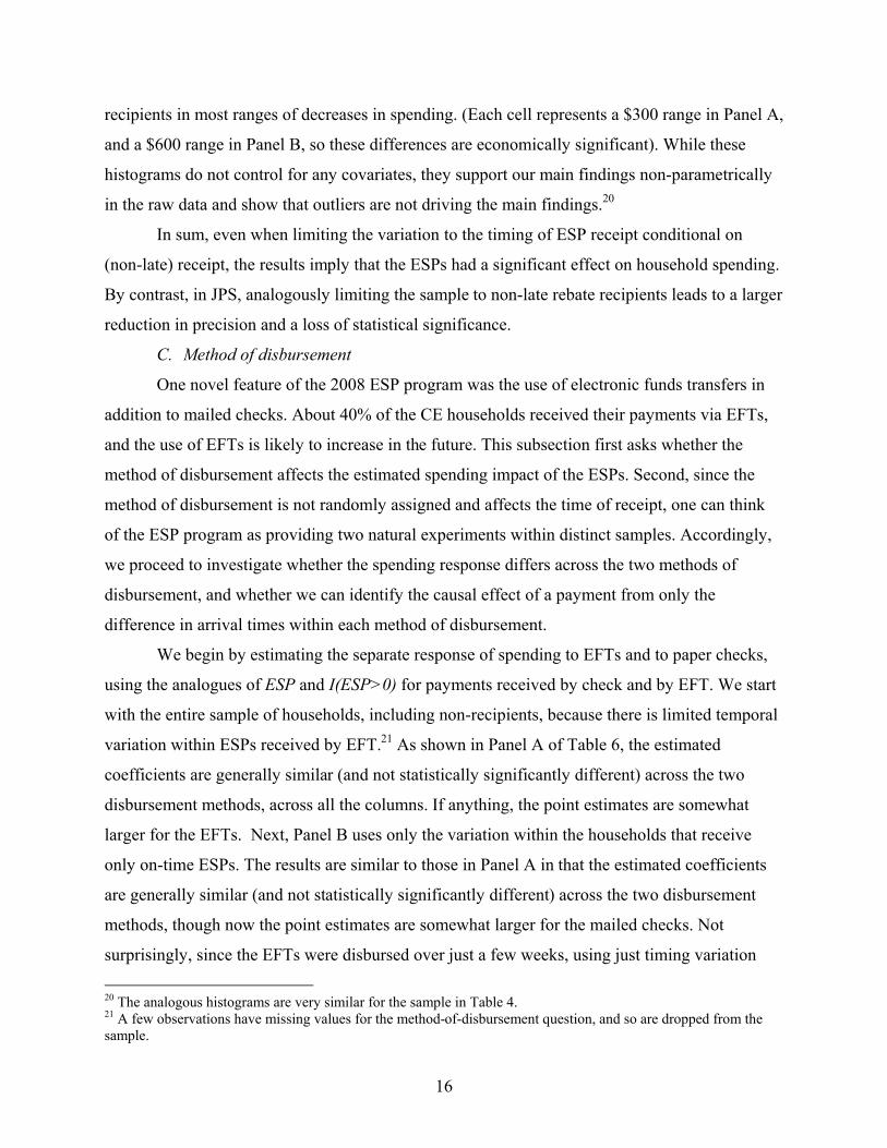
recipients in most ranges of decreases in spending. (Each cell represents a $300 range in Panel A,

and a $600 range in Panel B, so these differences are economically significant). While these

histograms do not control for any covariates, they support our main findings non-parametrically

in the raw data and show that outliers are not driving the main findings.20

In sum, even when limiting the variation to the timing of ESP receipt conditional on

(non-late) receipt, the results imply that the ESPs had a significant effect on household spending.

By contrast, in JPS, analogously limiting the sample to non-late rebate recipients leads to a larger

reduction in precision and a loss of statistical significance.

C. Method of disbursement

One novel feature of the 2008 ESP program was the use of electronic funds transfers in

addition to mailed checks. About 40% of the CE households received their payments via EFTs,

and the use of EFTs is likely to increase in the future. This subsection first asks whether the

method of disbursement affects the estimated spending impact of the ESPs. Second, since the

method of disbursement is not randomly assigned and affects the time of receipt, one can think

of the ESP program as providing two natural experiments within distinct samples. Accordingly,

we proceed to investigate whether the spending response differs across the two methods of

disbursement, and whether we can identify the causal effect of a payment from only the

difference in arrival times within each method of disbursement.

We begin by estimating the separate response of spending to EFTs and to paper checks,

using the analogues of ESP and I(ESP>0) for payments received by check and by EFT. We start

with the entire sample of households, including non-recipients, because there is limited temporal

variation within ESPs received by EFT.21 As shown in Panel A of Table 6, the estimated

coefficients are generally similar (and not statistically significantly different) across the two

disbursement methods, across all the columns. If anything, the point estimates are somewhat

larger for the EFTs. Next, Panel B uses only the variation within the households that receive

only on-time ESPs. The results are similar to those in Panel A in that the estimated coefficients

are generally similar (and not statistically significantly different) across the two disbursement

methods, though now the point estimates are somewhat larger for the mailed checks. Not

surprisingly, since the EFTs were disbursed over just a few weeks, using just timing variation

20 The analogous histograms are very similar for the sample in Table 4. 21 A few observations have missing values for the method-of-disbursement question, and so are dropped from the sample.

17

leads to relatively less power for estimating the effect of EFT receipt, especially for the noisier

total expenditure category. And the smaller number of ESPs used to identify the effects of a

mailed ESP also raise its standard errors. In sum, these results provide little evidence that the

method of disbursement significantly affected the average response of spending.

We now turn to the question of whether we can identify the spending effect using only

the randomized variation in spending within households that receive only on-time ESPs by check

and within households that receive only on-time ESPs by EFT. This approach allows for the

selection into each group to be non-random. For example, households receiving EFTs have

somewhat higher income on average than households receiving paper checks, and might also be

different in other, hard to observe ways (e.g., perhaps they are more technologically savvy).

Panels A and B, already discussed, provide some evidence that the spending effect does

not differ by method of disbursement. The coefficients in panel B in particular are identified

from variation within each group. Importantly, for ESPs received by mail, which provide more

temporal variation, the results are statistically significant and broadly similar to the average

response in the final panel of Table 5. That is, even separately controlling for receipt of EFTs,

using the random variation in the timing of the mailed checks still yields a significant response of

spending to the mailed checks.

These results still impose common month dummies and common demographic effects

(age and changes in family size) across EFT and mailed-check recipients. Also, to gauge the

impact of the stimulus program, we want to estimate the average response to the stimulus

payments. Accordingly, as an extension, Panel C of Table 6 presents estimates from a pooled

regression that allows for separate time dummies and demographic effects across three groups of

households: a) households who received only paper checks; b) households who received only

EFTs; c) households who received both paper checks and EFTs.22 The resulting coefficient

measures the average spending effect of the receipt of an ESP independent of its method of

disbursement, but allowing for households to be distributed across the different possible

disbursement methods in a way that is potentially correlated with their spending dynamics due to

other factors. While slightly smaller and less statistically significant, the estimates in Panel C 22 About 2 percent of households received both EFTs and paper checks. Across all the columns in Panel C, the coefficients on the time dummies (jointly) and the demographic variables (jointly) never significantly vary across the two main groups of households, those who received only EFTs and those who received only mailed checks. These coefficients are sometimes significantly different only for the few households who received both EFTs and paper checks, relative to the two main groups.

18

remain broadly similar to the previous estimates, even though they are driven only by the

randomized variation in timing within each group (primarily paper checks, since the EFTs have

limited timing variation).

In sum, our findings remain broadly consistent across specifications that use different

forms of variation. Of course, using different variation sometimes induces changes in the point

estimates across specifications, especially for total expenditures, but not significantly so relative

to the corresponding confidence intervals.

VI. The Longer-Run Response of Expenditure

To investigate the longer-run effect of the stimulus payments, we add the first lag of the

payment variable, ESPt, as an additional regressor in equation (1). We continue to focus on the

sample of households that only receive ESPs on time (as in Panel C of Table 5).

As shown in Table 7, the presence of the lagged variable does not much alter our

previous conclusions about the short-run impact of the payment, although the coefficients on

ESPt+1 are slightly smaller than the corresponding results in Panel C of Table 5. Moreover, the

receipt of a payment causes a change in spending one quarter later (i.e., from the three-month

period of receipt to the next three-month period) that uniformly is negative but smaller in

absolute magnitude than the contemporaneous change. Since the net effect of the payment on the

level of spending in the later quarter (relative to the level in the quarter before receipt) is given

by the sum of the coefficients on ESPt and ESPt+1, this implies that, after increasing in the three-

month period of payment receipt, spending remains high, though less high, in the subsequent

three-month period.

These lagged spending effects are, however, estimated with less precision than the

contemporaneous effects. For example, in the second-to-last column, for nondurable

expenditures using 2SLS, nondurable expenditures rise by 25.4% of the payment in the quarter

of receipt. The expenditure change in the next quarter is -9.7%, so that nondurable expenditures

in the second three-month period are still higher on net than before payment receipt by 25.4%-

9.7% ! 15.7% of the payment (penultimate row of results). The cumulative change in nondurable

expenditures over both three-month periods is then estimated to be 25.4% + 15.7% = 41.1% of

the payment (bottom row). However, neither the 15% change in the second period nor the 41%

cumulative change is statistically significant. The second-period and cumulative changes are also

19

insignificant in the other columns that use 2SLS. However, in the first triplet of columns, using

variation in the amount of the ESP increases statistical power, so that we find statistically

significant effects on spending in the second period for strictly nondurable goods, and on

cumulative spending for both strictly nondurable and nondurable expenditure.23

In sum, while the point estimates suggest some ongoing though decaying spending

response to the ESPs in the subsequent quarter after receipt, this lagged response cannot be

estimated with precision, even on average over the sample period. Hence, in the subsequent

extensions in which we estimate spending effects on subsamples of households and goods, which

reduces statistical power, we focus on the more precisely estimated short-run response.

VII. Differences in Responses across Households

This section and the next section analyze heterogeneity in the response to the stimulus

payment, across different types of households and different subcategories of consumption

expenditures, respectively. This analysis provides some evidence about why households’

expenditures respond to the payments. For brevity, we report results from the 2SLS specification,

instrumenting the payment ESP (and any interaction terms) with the corresponding indicator

variables for payment receipt I(ESP>0) (and their interactions, along with the other independent

variables), for the sample of households receiving only non-late payments.

A. Spending propensities by age, income and liquid wealth

The presence of liquidity constraints is a leading explanation for why household spending

might increase in response to a previously announced increase in income. To investigate this

explanation, we test whether households that were relatively likely to be constrained were more

likely to increase their spending upon the arrival of a payment. Constrained households may be

unable or unwilling to increase their spending prior to the payment arrival. On the other hand,

unconstrained households (e.g., high wealth or high income households) may find the costs of

not smoothing consumption across the arrival of the payment to be small (Caballero, 1995;

Parker, 1999; Sims, 2003; and Reis, 2006).

Expanding equation (1), we interact the intercept and ESPt+1 variable with indicator

variables (Low and High) based on various household characteristics (all from households’ first

23 The coefficients are generally slightly smaller and the statistical significance slightly lower in the sample comprised of all households.

20

CE expenditure interview to minimize any endogeneity). We use three different proxy variables

to identify households that may be disproportionately likely to be liquidity constrained: age,

income (family income before taxes), and liquid assets (the sum of balances in checking and

saving accounts). While liquid assets is arguably the most directly relevant of these variables for

identifying liquidity constraints, it is the least well measured and the most often missing in the

CE data, so we start with the other two variables.24 For each variable, we split households into

three groups (Low, High, and the intermediate baseline group), with the cutoffs between groups

chosen to include about a third of the payment recipients in each group.

Table 8 begins by testing whether the propensity to spend the stimulus payments differs

by age. Because young households typically have low liquid wealth and high income growth,

they are disproportionately likely to be liquidity constrained (e.g., Jappelli, 1990; Jappelli et. al.,

1998).25 In the first set of columns in the table, Low refers to young households (40 years old or

younger) and High refers to older households (older than 58), and the coefficients on the

interaction terms with these variables represent differences relative to the households in the

baseline, middle-age group. As reported, the point estimates for the interaction terms suggest that

young households spent relatively less of the payment and old households spent relatively more.

However these differences, while economically large, are not statistically significant.

Nonetheless, in absolute terms the spending by old households (see bottom panel for the

interacted groups) and by the middle-age households (main panel for the baseline group) are both

statistically and economically significant.

The second set of columns in Table 8 tests for differences in spending across income

groups. The point estimates suggest that low-income households spent a much larger fraction of

their payment on total expenditures relative to the typical (baseline middle-income) household.

In absolute terms for total expenditures, of the three groups, only the response for the low-

income households is statistically significant. The response is also economically significant,

averaging about 125% of the payment.26 However, while suggestive of possible role for liquidity

24 The CE survey does not include the direct measures of borrowing and credit constraints used by Jappelli (1990) and Jappelli et. al. (1998), or Agarwal, Liu, and Souleles (2007). 25 There is also evidence that some older households increase their spending on receiving their (predictable) pension checks (Wilcox, 1989; and Stephens, 2003). Outside the null LCPIH hypothesis of "2=0, older households might also spend relatively more because they have shorter time horizons on average. 26 It is not inconsistent for the average spending response to be larger in magnitude than the average payment, even putting aside the confidence intervals for the former, if enough households buy large durables like autos in response to receiving a payment, as found below.

21

constraints, the difference between this result and that for the baseline group, although

economically large at about 70% of the ESP, is not statistically significant.

The last set of columns in Table 8 tests for differences by liquid asset holdings. While the

point estimates suggest little spending by low-asset households, the associated confidence

interval is quite large, and none of the differences (although large in point estimate) are

statistically significant. Indeed, even the total amounts of spending in absolute terms are

insignificant for all three groups, for both nondurable expenditures and total expenditures. The

loss of precision when using the asset variable might reflect the smaller sample sizes due to

missing asset values and measurement error in the available asset values.

One possible complication in assessing liquidity constraints during the sample period is

that households might have expected the recent recession to last longer than usual. For instance,

if constrained households expect their constraints to bind for a year or two after receiving a

payment, rather than for just a few months, this would reduce the magnitude of their current

response to the payment.

B. Spending propensities by homeownership status

Another key characteristic of the recent recession was the large decline in housing wealth

and the reduced ability to borrow against home equity. To examine the potential implications for

the response to the ESPs, Table 9 presents estimates of the spending responses according to

housing status. The baseline group is renters (23% of the sample), and the two interacted groups

are homeowners with a mortgage (50%) and homeowners without a mortgage (27%). The point

estimates suggest much larger spending responses by both groups of homeowners relative to

renters, though the differences are not statistically significant. In absolute terms, homeowners

have large and significant responses for all three expenditure categories, whereas the response of

renters is smaller and insignificant. As an extension, combining homeowners into one group, the

estimated spending responses for total expenditures are 1.051 (0.351) for homeowners and 0.434

(0.454) for renters, and these estimates are statistically significantly different at the 10 percent

level.27

27 The results for homeowners do not simply reflect the preceding results for older households. E.g., if one drops from the sample the households older than 65, the coefficients for nondurable expenditure remain very similar to those reported in Table 9, for all three groups of homeowner status. The coefficients for total expenditure remain very similar for renters and homeowners with mortgages. While the coefficient for total expenditure loses significance for homeowners without mortgages, presumably in part due to the reduced sample of such homeowners,

22

C. Spending propensities by self-reported spending propensities

Finally, we evaluate the alternative methodological approach that identifies the impact of

tax cuts by asking consumers to self-report whether they spent their tax cut. In our sample of on-

time ESP recipients, 32% reported that they mostly spent their payment, 18% reported they

mostly saved it, and 50% reported they mostly used it to pay down debt.28 We interact ESP with

indicator variables for self-reports of mostly spend and of mostly pay down debt, with mostly

save being the baseline category.

Supporting the use of self-reports, Table 10 shows that households reporting that they

mostly spent their ESPs did in fact spend more of the payment than the other groups, according

to the point estimates. In absolute terms their spending is statistically and economically

significant, across all the expenditure categories. In relative terms, they spent about 35% more of

the payment on nondurable expenditures than the baseline group, the self-reported savers, and

this difference is statistically significant. The corresponding difference for total expenditures is

even larger in magnitude, at 75% of the ESP on average, but is not statistically significant.

On the other hand, even for the self-reported “non-spenders,” the receipt of an ESP

caused significant spending. For self-reported savers, the response of total expenditures is

statistically significant and large at 95% of the payment on average. For households who

reported they paid down debt, the response of total expenditures is still large at about 63%, albeit

statistically insignificant, and the response of nondurable expenditures is statistically significant

and still rather large at 27% of the payment. In this sense self-reported spending may understate

the actual amount of spending (see also Agarwal, Liu, and Souleles, 2007).

VIII. Differences in Responses across Types of Expenditure

Turning to differences across types of expenditures, each column in Table 11 reports the

estimated change in spending for each subcategory of expenditures within the broad measure of

nondurable expenditures (a complete decomposition). The columns also report, in the bottom

panel, the share of the estimated overall increase in nondurable expenditures due to the ESPs that

is accounted for by each of the subcategories, and for benchmarking, the average share of each

it remains large in magnitude; and as in the table, the coefficient for nondurable expenditure remains significant and is largest for homeowners without mortgages, compared to the other two groups. 28 These results are very close to those in Bureau of Labor Statistics (2009), reported above, which used the entire sample of data on self-reported usage, without considering its relation to actual spending.

23

subcategory in nondurable expenditures. Of course, comparisons of different subsets of

nondurable expenditure must be interpreted cautiously because of potential non-separabilities

across goods.

Further, note that in general the results are statistically weak, with only the estimated

coefficient for utilities and household operations being statistically significant. This response is

roughly in proportion to the share of this subcategory in nondurable expenditures. As for the

other categories, the point estimates suggest a disproportionately large response in alcohol,

personal care (and miscellaneous items), tobacco, and apparel, though these responses are

nonetheless statistically insignificant. For such narrow subcategories of expenditures there is

much more variability in the dependent variable that is unrelated to the payment regressor. Our

previous results, by summing the subcategories into broader aggregates of nondurable

expenditures, averaged out much of this unrelated variability (such as, for example, whether a

trip to the supermarket happened to fall just inside or outside the expenditure reference-period).

Panel A of Table 12 provides the analogous decomposition of the response of the

durable goods and services part of total expenditures (i.e., the part of total expenditures not in the

nondurables category). While there are sizable responses on average in housing (which includes

shelter and furniture/appliances) and entertainment (which includes TVs and other electronic

equipment), these responses are statistically insignificant and not large relative to their category

share in durable goods. The bulk of the response in durables comes in transportation, spending

on which increases by 53% of the payments on average, a statistically and economically

significant amount. This response is large in light of the small average share of transportation in

durable expenditures. Panel B in turn decomposes the response of the different subcategories of

transportation. According to the point estimates, the transportation response is largely driven by

purchases of vehicles, primarily new vehicles. These results imply that auto purchases, although

weakening during the recession, would have been even weaker in the absence of the payments.

In sum, receipt of a stimulus payment increased the probability of purchasing a vehicle,

relative to the counterfactual of no payment, and such purchases are large enough in magnitude

that they imply large average responses of total expenditures to the payments.

24

IX. Conclusion

We find that on average households spent about 12-30% of their stimulus payments,

depending on the specification, on (CE-defined) nondurable expenditures during the three-month

period in which the payments were received. This response is larger than implied by the LCPIH

or Ricardian equivalence. We also find a significant effect on the purchase of durable goods,

primarily the purchase of new vehicles, bringing the average response of total consumption

expenditures to about 50-90% of the payments in the quarter of receipt. These results are

statistically and economically significant. They remain broadly consistent and significant across

specifications that use different forms of variation. Indeed, the point estimates are at the high end

of these ranges in specifications that focus most directly on randomized timing variation.

For nondurable expenditures, the estimated spending response to the 2008 EPSs is

generally only slightly smaller in magnitude (and not significantly different) than the response to

the 2001 tax rebates. This difference might partly reflect the more transitory nature of the 2008

tax cut. However, the composition of spending is different than in 2001, so that the estimated

spending effect on total expenditures is larger than that in 2001 due to a larger role for durables

in 2008. This difference might reflect the larger size of the payments in 2008.

We also find some evidence of an ongoing though smaller response in the subsequent

three-month period after ESP receipt, but this response cannot be estimated with precision.

These estimates suggest a significant macroeconomic effect of the 2008 ESPs on

consumer demand. To give a sense of the effect, we calculate alternative paths for aggregate

consumption that subtract the direct spending caused by the ESPs, as implied by our point

estimates and the monthly pattern of distribution of the ESPs. In Figure 3, the (blue) solid line

shows the National Income and Product Accounts measure of actual total aggregate PCE from

the third quarter of 2007 to the second quarter of 2009. The dashed lines show this series less

estimates of the direct spending effect of the ESP program from different specifications used in

the paper. In all cases the implied effects of the ESPs are economically significant.

Quantitatively, our preferred point estimates for total expenditures from Tables 4 and 5 imply

that the ESPs increased PCE by about 1.3 to 2.3 percent in 2008Q2 and 0.6 to 1.0 percent in

2008Q3 (at annual rates). Of course, this accounting exercise does not include any potential

effects of resource constraints and multiplier effects, but instead simply reveals the magnitude of

the direct aggregate demand effect relative to total PCE.

25

Regarding the implementation of new method of delivering tax cuts, the estimated

responses do not significantly differ across paper checks and electronic transfers.

Across households, the responses are largest for older and low-income households,

groups which have substantial and statistically significant spending responses. According to the

point estimates, the responses are largest for high-asset households but this spending response is

not statistically significantly different from zero, and more generally all of the asset results suffer

from a lack of statistical power. Also, homeowners are estimated to have higher spending

propensities than renters.

Finally, the responses are largest for self-reported spenders, supporting the

informativeness of surveys that elicit self-reported usage. However, self-reported savers

(including those reporting they reduced debt) also spent a statistically and economically

significant fraction of their payments, suggesting that relying on self-reports can understate the

actual amount of spending.

26

Appendix A: A notification letter for an ESP by electric funds transfer

27

Appendix B: The 2008 ESP Survey Instrument

a) The following questions were asked in all CE interviews in June 2008 – March 2009: [Earlier this year/Last year] the Federal government approved an economic stimulus package. [Many households will receive a one-time economic stimulus payment, either by check or direct deposit/Previously you or your CU [[consumer unit]] reported receiving one or more economic stimulus payments.] This is also called a tax rebate and is different from a refund on your annual income taxes. Since the first of the reference month, have you or any members of your CU received a/an additional 10. Tax rebate? [Economic Stimulus Payment] 99. None/No more entries Who was the rebate for? [enter text] _____________ * Collect each rebate separately and include the name(s) of the recipient(s). In what month did you receive the rebate? [enter text] _____________ What was the total amount of the rebate? [enter value] _____________ * Probe if the amount is not an expected increment such as $300, $600, $900, $1,200, etc Was the rebate received by - ? 1. check? 2. direct deposit? Did you or any members of your CU receive any other tax rebate [economic stimulus payment]? 1. Yes 2. No If yes, return to “Who was the tax rebate for?” b) The following question was asked (during June 2008 – March 2009) of households that previously reported receiving an economic stimulus payment. Once the question was answered, it was not asked again. [Earlier in this interview/Last interview/Previously] [you/your consumer unit] reported receiving a one-time tax rebate that was part of the Federal government's economic stimulus package. Did the tax rebate lead [you/your consumer unit] mostly to increase spending, mostly to increase savings, or mostly to pay off debt?

1. mostly to increase spending 2. mostly to increase saving 3. mostly to pay off debt

28

Appendix C: The CE Data

We construct the economic stimulus payment variable ESP from the CE ESP data

(Appendix A) in a similar manner to JPS’s construction of the 2001 tax rebate variable. The

2008 data require fewer consistency checks and adjustments, however. This is partly because by

2008 the CE survey used CAPI software to input and cross-check respondents’ replies.

Moreover, with a few exceptions, each interview records only ESPs received during the months

of the interview’s reference period. We adjusted the exceptions to bring their payments into the

appropriate consumption reference period.

We use the following definitions of the other main variables. Age is the average age of

the head and spouse when the household is a married couple, otherwise it is just the age of the

head. The number of children is calculated as the number of members of the household younger

than 18.

Following Lusardi (1996), strictly nondurable expenditures include expenditures on food

(away from home, at home and alcoholic beverages), utilities (and fuels and public services),

household operations, public transportation and gas and motor oil, personal care, tobacco, and

miscellaneous goods. Nondurable expenditures (broadly defined) adds spending on apparel

goods and services, health care (excluding payments by employers or insurers), and reading

materials, following Lusardi (1996) but excluding education. Total expenditure adds spending on

education, housing (including furniture and appliances and shelter but excluding utilities and

household operations, which are already included in nondurable expenditures), transportation

(including vehicle purchases, maintenance, and insurance, but excluding public transportation

and gas and motor oil), and entertainment (e.g., including TVs and other electronics, as well as

fees).

Turning to the sample, we omit observations missing any of the key data that we use in

our regressions. Our sample omits the bottom one percent of nondurable consumption

expenditures in levels (after adjusting for family size and allowing for a time trend), since this

data implies implausibly small (often negative) consumption expenditures. Finally, we drop

household observations that report living in student housing, that report age less than 21 or

greater than 85, that report age changing by more than one or a negative amount between

quarters, or that report changes in the number of children or adults greater than three in absolute

magnitude. When we split the sample based on income, we drop households flagged as

29

incompletely reporting income. When we split based on liquid assets, we drop households if the

asset information used in computing initial assets (as the difference between final assets and the

change in assets) is topcoded.

30

References

Adams, William, Einav, Liran, and Levin, Jonathan, 2009, “Liquidity Constraints and Imperfect

Information in Subprime Lending,” American Economic Review, 99(1), March, pp. 49-84.

Agarwal, Sumit; Liu, Chunlin and Souleles, Nicholas S., 2007, “The Response of Consumer

Spending and Debt to Tax Rebates – Evidence from Consumer Credit Data,” Journal of

Political Economy, 115(6), December, pp. 986-1019.

Auerbach, Alan J., and Gale, William G., 2009, “Activist Fiscal Policy to Stabilize Economic

Activity,” working paper, September.

Barrow, Lisa, and McGranahan, Leslie, 2000, “The Effects of Earned Income Credit on the

Seasonality of Household Expenditures,” National Tax Journal, December, 53, pp. 1211-44.

Bertrand, Marianne, and Morse, Adair, 2009, What do High-Interest Borrowers Do with their

Tax Rebate?” American Economic Review (Papers and Proceedings), May.

Broda, Christian, and Parker, Jonathan, 2008, “The Impact of the 2008 Tax Rebates on

Consumer Spending: Preliminary Evidence,” working paper, July.

Browning, Martin and Lusardi, Annamaria, 1996, “Household Saving: Micro Theories and

Macro Facts,” Journal of Economic Literature, 34(4), pp 1797-1855.

Bureau of Labor Statistics, U.S. Department of Labor, 2009, “Consumer Expenditure Survey

Results on the 2008 Economic Stimulus Payments (Tax Rebates),” October,

(http://www.bls.gov/cex/taxrebate.htm).

Caballero, Ricardo J., 1995, “Near Rationality, Heterogeneity, and Aggregate Consumption,”

Journal of Money, Credit, and Banking, February, 27(1), pp. 29-48.

CCH, 2008, “CCH Tax Briefing: Economic Stimulus Package,” February 13.

Chamberlain, Gary, 1984, “Panel Data,” in Griliches, Zvi, and Intriligator, Michael D., eds.,

Handbook of Econometrics, Amsterdam: North-Holland.

Coronado, Julia Lynn, Lupton, Joseph P., and Sheiner, Louise M., 2006, “The Household

Spending Response to the 2003 Tax Cut: Evidence from Survey Data,” working paper.

Deaton, Angus, 1992, Understanding Consumption, Oxford: Clarendon Press.

Jappelli, Tullio, 1990, “Who is Credit Constrained in the U.S. Economy?” Quarterly Journal of

Economics, February, 105, pp. 219-234.

Jappelli , Tullio and Luigi Pistaferri, 2010, “The Consumption Response to Income Changes,”

NBER Working Paper 15739, February.

31

Jappelli, Tullio, Pischke, Jörn-Steffen, and Souleles, Nicholas S., 1998, “Testing for Liquidity

Constraints in Euler Equations with Complementary Data Sources,” The Review of

Economics and Statistics, 80, pp. 251-262.

Johnson, David S., Parker, Jonathan A., and Souleles, Nicholas S., 2006, “Household

Expenditure and the Income Tax Rebates of 2001,” American Economic Review, 96, pp.

1589-1610.

Johnson, David S., Parker, Jonathan A., and Souleles, Nicholas S., 2009, “The Response of

Consumer Spending to Rebates During an Expansion: Evidence from the 2003 Child Tax

Credit,” working paper, April.

Lusardi, Annamaria, 1996, “Permanent Income, Current Income, and Consumption: Evidence

from Two Panel Data Sets,” Journal of Business Economics and Statistics, January, 14(1),

pp. 81-90.

Parker, Jonathan A., 1999, “The Reaction of Household Consumption to Predictable Changes in

Social Security Taxes,” American Economic Review, September, 89(4), pp. 959-973.

Reiss, Ricardo, 2006, “Inattentive Consumers,” Journal of Monetary Economics, 53(8), pp.

1761-80.

Sahm, Claudia R., Shapiro, Matthew D. and Slemrod, Joel B., 2010, “Household Response to the

2008 Tax Rebates: Survey Evidence and Aggregate Implications,” in Tax Policy and The

Economy, ed. Jeffrey R. Brown, Cambridge: MIT Press.

Shapiro, Matthew D. and Slemrod, Joel B., 2003a, “Consumer Response to Tax Rebates,”

American Economic Review, 85, pp. 274-283.

Shapiro, Matthew D., and Slemrod, Joel B., 2003b, “Did the 2001 Tax Rebate Stimulate

Spending? Evidence from Taxpayer Surveys,” Tax Policy and the Economy, ed. James

Poterba, Cambridge: MIT Press.

Shapiro, Matthew W. and Slemrod, Joel B., 2009, “Did the 2008 Tax Rebates Stimulate

Spending?” American Economic Review, May, 99(2), pp. 374-79.

Sims, Christopher A., 2003, “Implications of Rational Inattention,” Journal of Monetary

Economics, April, 50(3), pp. 665-690.

Slemrod, Joel B., Christian, Charles, London, Rebecca, and Parker, Jonathan A., 1997, “April 15

Syndrome,” Economic Inquiry, October, 35(4), pp. 695-709.

32

Souleles, Nicholas S., 1999, “The Response of Household Consumption to Income Tax

Refunds,” American Economic Review, September, 89(4), pp. 947-958.

Souleles, Nicholas S., 2004, “Expectations, Heterogeneous Forecast Errors, and Consumption:

Micro Evidence from the Michigan Consumer Sentiment Surveys,” Journal of Money,

Credit, and Banking, February, 36 (1), pp. 39-72.

Stephens, Melvin, Jr., 2003, “3rd of tha Month: Do Social Security Recipients Smooth

Consumption Between Checks?” American Economic Review, 93, pp. 406-422.

Department of the Treasury, “Daily Treasury Statement,” Washington: GPO, 2008, various

issues.

Wilcox, David W., 1989, “Social Security Benefits, Consumption Expenditures, and the Life

Cycle Hypothesis,” Journal of Political Economy, 97, pp. 288-304.

Zeldes, Stephen P., 1989, “Consumption and Liquidity Constraints: An Empirical Investigation,”

Journal of Political Economy, 97, pp. 305-346.

!

Table 1: The timing of the economic stimulus payments

Last two digits of taxpayer SSN

Date ESP funds transferred to

account byLast two digits of

taxpayer SSNDate ESP check in

the mail by

00 – 20 May 2 00 – 09 May 16

21 – 75 May 9 10 – 18 May 23

76 – 99 May 16 19 – 25 May 30

26 – 38 June 6

39 – 51 June 13

52 – 63 June 20

64 – 75 June 27

76 – 87 July 4

88 – 99 July 11

Source: Internal Revenue Service (http://www.irs.gov/newsroom/article/0,,id=180247,00.html)

Panel A: Payments by electronic funds transfer

Panel B: Payments by paper check

Table 2: Sample statistics

Sample:Variable Mean (std dev) Mean (std dev) Mean (std dev) Mean (std dev)Expenditures on: Food 1,902 (1,356) 1,910 (1,305) 1,792 (1,336) 2,045 (1,176) Strictly nondurables 4,298 (2,657) 4,361 (2,440) 4,077 (2,418) 4,690 (2,304) Nondurables 5,342 (3,296) 5,461 (2,973) 5,090 (2,943) 5,901 (2,827) Total 10,492 (8,124) 10,591 (7,228) 9,694 (6,999) 11,713 (7,162) Change in Expenditures on: Food 7.7 (1,130) 12.7 (1,115) 16.8 (1,164) 6.2 (1,018) Strictly nondurables 59.0 (1,918) 59.1 (1,820) 48.4 (1,807) 73.3 (1,796) Nondurables 46.7 (2,279) 49.3 (2,180) 38.2 (2,174) 62.1 (2,148) Total -87.5 (7,361) -80.9 (7,165) -36.3 (6,675) -153.6 (7,628) Level of: Number of Adults 1.9 (0.8) 1.9 (0.8) 1.9 (0.8) 1.9 (0.7) Number of Children 0.7 (1.1) 0.8 (1.1) 0.7 (1.1) 0.9 (1.1)Change in: Number of Adults 0.0 (0.24) 0.0 (0.23) 0.0 (0.24) 0.0 (0.23) Number of Children 0.0 (0.19) 0.0 (0.19) 0.0 (0.20) 0.0 (0.18)Age 48.4 (14.9) 48.5 (14.8) 50.6 (15.4) 45.4 (13.2)

ESP 215 (472) 307 (538) 284 (496) 332 (581)I(ESP>0) 0.23 (0.42) 0.32 (0.47) 0.32 (0.47) 0.31 (0.46)ESP | ESP>0 (N=690) 960 (520) 971 (518) 899 (490) 1082 (527)

Income 74,770 (148,814) 66,387 (108,738) 58,153 (103,035) 77,310 (112,638) Liquid Assets 9,553 (20,193) 9,959 (20,145) 9,244 (19,454) 11,165 (21,466)

Notes: The first two samples correspond to those used in Table 4 and Table 5 Panel C. The final two samples together with households that receive payments both by electronic transfer of funds and by check, comprise the sample used in Table 6 Panels B and C. The samples used to calculate income and liquid assets data include only households with valid information on these variables and so are subsamples of the samples used in these tables. For the income and assets variables, the on-time recipients sample corresponds to the samples used in the final two triplets of columns in Table 8.

Households with onlyon-time ESPs by check

Households with onlyon-time ESPs by EFTOn-time recipientsFull sample

Table 3: The distribution of reported economic stimulus payments

Sample:

Percent of Percent of Percent ofESP value Number ESPs Number ESPs Number ESPs0<ESP<300 47 1.5 26 1.6 10 1.0ESP=300 343 11.2 220 13.1 69 6.8300<ESP<600 77 2.5 40 2.4 16 1.6ESP=600 943 30.9 558 33.3 278 27.3600<ESP<900 52 1.7 31 1.8 13 1.3ESP=900 168 5.5 99 5.9 55 5.4900<ESP<1200 42 1.4 27 1.6 11 1.1ESP=1200 800 26.2 440 26.3 287 28.21200<ESP<1500 27 0.9 15 0.9 9 0.9ESP=1500 213 7.0 88 5.3 104 10.21500<ESP<1800 25 0.8 11 0.7 12 1.2ESP=1800 195 6.4 74 4.4 99 9.71800<ESP<2100 7 0.2 1 0.1 4 0.4ESP=2100 63 2.1 25 1.5 31 3.02100<ESP<2400 4 0.1 0 0.0 4 0.4ESP=2400 23 0.8 9 0.5 9 0.92400<ESP<2700 1 0.0 1 0.1 0 0.0ESP=2700 7 0.2 4 0.2 2 0.22700<ESP<3000 2 0.1 1 0.1 1 0.1ESP=3000 10 0.3 4 0.2 4 0.4ESP>3000 3 0.1 2 0.1 0 0.0

Mean Num (%) of obs Mean Num (%) of obs Mean Num (%) of obsExpenditure Period ESP| ESP >0 with ESP>0 ESP| ESP >0 with ESP>0 ESP| ESP >0 with ESP>0Mar - May, 2008 1,021 467 (33) 858 136 (33) 1,091 308 (88)Apr - June, 2008 1,009 780 (57) 932 397 (76) 1,091 341 (100)May - July, 2008 973 924 (68) 909 572 (98) 1,071 298 (100)June- Aug, 2008 891 539 (39) 867 398 (78) 1,043 71 (20)July - Sept, 2008 875 223 (16) 917 151 (28) - 0 (0)Aug - Oct, 2008 811 62 (5) 735 22 (4) - 0 (0)Sept - Nov, 2008 703 22 (2) - 0 (0) - 0 (0)Oct - Dec, 2008 703 20 (1) - 0 (0) - 0 (0)Nov - Jan, 2009 890 11 (1) - 0 (0) - 0 (0)Dec - Feb, 2009 435 4 (0) - 0 (0) - 0 (0)Notes: The first sample corresponds to that used in Table 4. The second and third samples together with households that receive payments both by electronic funds transfer and by check, comprise the sample used in Table 6 Panel C.

Full sampleHouseholds with only on-

time ESPs by checkHouseholds with only on-

time ESPs by EFT

Panel B: by expenditure period

Panel A: by amount of ESP

Table 4: The contemporaneous response of expenditures to the ESPs among all households

DependentVariable:

Food Strictly Non-

durables

Non-durable

spending

Total spending

Food Strictly Non-

durables

Non-durable

spending

Total spending

Food Strictly Non-

durables

Non-durable

spending

Total spending

Food Strictly Non-

durables

Non-durable

spending

Total spending

Estimationmethod: OLS OLS OLS OLS OLS OLS OLS OLS OLS OLS OLS OLS 2SLS 2SLS 2SLS 2SLS

ESP 0.016 0.079 0.121 0.516 0.012 0.079 0.128 0.523(0.027) (0.046) (0.055) (0.179) (0.033) (0.060) (0.071) (0.219)

I(ESP) 10.9 74.8 121.5 494.5 0.69 1.74 2.09 3.24(31.7) (56.6) (67.2) (207.2) (1.27) (0.96) (0.94) (1.17)

Age 0.72 -0.23 0.96 6.56 0.70 -0.35 0.77 5.77 0.048 0.009 0.029 0.045 0.70 -0.20 1.00 6.60(0.34) (0.65) (0.81) (2.25) (0.34) (0.65) (0.81) (2.24) -0.010 -0.010 -0.010 -0.010 (0.30) (0.60) (0.80) (2.30)

Change in 198 448 561 452 198 448 561 452 8.96 8.43 8.99 4.78 198 448 561 453 # adults (55) (106) (118) (375) (55) (106) (118) (375) (1.77) (1.34) (1.32) (1.63) (55) (106) (118) (375)

Change in 89 139 185 -254 89 139 186 -252 4.50 3.35 3.93 1.42 89 139 185 -254 # children (48) (96) (111) (388) (48) (96) (111) (388) (2.02) (1.53) (1.50) (2.10) (48) (96) (111) (388)

Num of obs 17,478 17,478 17,478 17,478 17,478 17,478 17,478 17,478 17,427 17,475 17,478 17,478 17,478 17,478 17,478 17,478

Dollar change in Dollar change in Percent change in Dollar change in

Notes: All regressions also include a full set of month dummies, following equation (1). Reported standard errors are adjusted for arbitrary within-household correlations and heteroskedasticity. The coefficients in the third set of columns are multiplied by 100 so as to report a percent change. The last four columns report results from 2SLS regressions where the indicator variable for ESP receipt and the other regressors are used as instruments for the amount of the ESP.

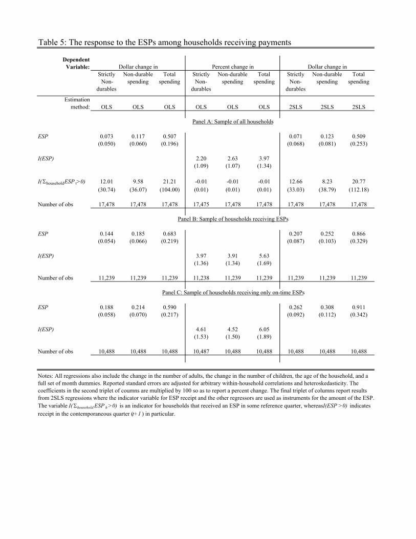
Table 5: The response to the ESPs among households receiving payments

Strictly Non-

durables

Non-durable spending

Total spending

StrictlyNon-

durables

Non-durable spending

Total spending

StrictlyNon-

durables

Non-durable spending

Total spending

Estimation method: OLS OLS OLS OLS OLS OLS 2SLS 2SLS 2SLS

ESP 0.073 0.117 0.507 0.071 0.123 0.509(0.050) (0.060) (0.196) (0.068) (0.081) (0.253)

I(ESP) 2.20 2.63 3.97(1.09) (1.07) (1.34)

I(!householdESP t>0) 12.01 9.58 21.21 -0.01 -0.01 -0.01 12.66 8.23 20.77(30.74) (36.07) (104.00) (0.01) (0.01) (0.01) (33.03) (38.79) (112.18)

Number of obs 17,478 17,478 17,478 17,475 17,478 17,478 17,478 17,478 17,478

ESP 0.144 0.185 0.683 0.207 0.252 0.866(0.054) (0.066) (0.219) (0.087) (0.103) (0.329)

I(ESP) 3.97 3.91 5.63(1.36) (1.34) (1.69)

Number of obs 11,239 11,239 11,239 11,238 11,239 11,239 11,239 11,239 11,239

ESP 0.188 0.214 0.590 0.262 0.308 0.911(0.058) (0.070) (0.217) (0.092) (0.112) (0.342)

I(ESP) 4.61 4.52 6.05(1.53) (1.50) (1.89)

Number of obs 10,488 10,488 10,488 10,487 10,488 10,488 10,488 10,488 10,488

Dependent Variable: Dollar change in Percent change in Dollar change in

Panel B: Sample of households receiving ESPs

Panel C: Sample of households receiving only on-time ESPs

Notes: All regressions also include the change in the number of adults, the change in the number of children, the age of the household, and a full set of month dummies. Reported standard errors are adjusted for arbitrary within-household correlations and heteroskedasticity. The coefficients in the second triplet of coumns are multiplied by 100 so as to report a percent change. The final triplet of columns report results from 2SLS regressions where the indicator variable for ESP receipt and the other regressors are used as instruments for the amount of the ESP. The variable I(!household ESP h >0) is an indicator for households that received an ESP in some reference quarter, whereas I(ESP >0) indicates receipt in the contemporaneous quarter (t+1 ) in particular.

Panel A: Sample of all households

Table 6: The response to the ESPs by method of disbursement

DependentVariable:

Strictly Non-

durables

Non-durable

spending

Total spending

StrictlyNon-

durables

Non-durable

spending

Total spending

StrictlyNon-

durables

Non-durable

spending

Total spending

Estimation method: OLS OLS OLS OLS OLS OLS 2SLS 2SLS 2SLS

ESP by Check 0.104 0.141 0.473 0.060 0.112 0.333(0.064) (0.077) (0.215) (0.087) (0.104) (0.305)

ESP by EFT 0.086 0.144 0.583 0.108 0.169 0.661(0.066) (0.081) (0.305) (0.083) (0.097) (0.332)

I(ESP by check) 1.92 2.19 3.59(1.31) (1.29) (1.61)

I(ESP by EFT) 2.81 3.35 4.00(1.44) (1.41) (1.83)

Number of obs 17,281 17,281 17,281 17,278 17,281 17,281 17,281 17,281 17,281

ESP by Check 0.220 0.245 0.746 0.257 0.308 0.868(0.072) (0.086) (0.235) (0.110) (0.133) (0.379)

ESP by EFT 0.188 0.218 0.361 0.281 0.313 0.702

Dollar change in Dollar change in

Panel B: Sample of households receiving only on-time ESPs

Panel A: Sample of all households

Percent change in

y(0.071) (0.090) (0.317) (0.095) (0.117) (0.402)

I(ESP by check) 4.13 3.99 5.78(1.67) (1.63) (2.03)

I(ESP by EFT) 5.19 4.84 4.30(1.83) (1.81) (2.38)

Number of obs 10,362 10,362 10,362 10,361 10,362 10,362 10,362 10,362 10,362

ESP 0.187 0.211 0.529 0.240 0.262 0.784(0.066) (0.078) (0.232) (0.128) (0.149) (0.401)

I(ESP) 3.96 3.63 5.48(1.87) (1.79) (2.23)

Number of obs 10,362 10,362 10,362 10,361 10,362 10,362 10,362 10,362 10,362

Notes: All regressions also include the change in the number of adults, the change in the number of children, the age of the household, a full set of month dummies, and indicators for: a) receiving only ESPs by check; b) receiving only EFTs; and c) receiving both checks and EFTs. In panels B and C, there are also separate sets of all other control variables for households in categories a), b), and c). Reported standard errors are adjusted for arbitrary within-household correlations and heteroskedasticity. The coefficients in the second triplet of coumns are multiplied by 100 so as to report a percent change. The final triplet of columns reports results from 2SLS regressions where I(ESP>0), its interactions, and the other regressors are used as instruments for ESP and its interactions.

Panel C: Households receiving only on-time ESPs, allowing different effect of all non-ESP regressors by disbursement method

Table 7: The longer-run response of expenditures to the ESPs

Strictly Non-

durables

Non-durable

spending

Total spending

StrictlyNon-

durables

Non-durable

spending

Total spending

StrictlyNon-

durables

Non-durable

spending

Total spending

Estimation method: OLS OLS OLS OLS OLS OLS 2SLS 2SLS 2SLS

ESP t+1 or I(ESP t+1 ) 0.186 0.201 0.517 3.58 3.92 4.96 0.219 0.254 0.757(0.055) (0.067) (0.211) (1.58) (1.55) (1.96) (0.089) (0.110) (0.360)

ESP t or I(ESP t ) -0.009 -0.054 -0.288 -2.09 -1.23 -2.22 -0.076 -0.097 -0.278(0.068) (0.080) (0.214) (1.51) (1.50) (1.92) (0.092) (0.113) (0.330)

Implied spending effect in 0.177 0.147 0.229 NA NA NA 0.143 0.157 0.479second three-month period (0.087) (0.104) (0.303) (0.142) (0.178) (0.568)

Implied cumulative fractionof rebate spent over both 0.363 0.348 0.746 NA NA NA 0.362 0.411 1.236

three-month periods (0.128) (0.155) (0.477) (0.218) (0.273) (0.892)

Number of observations 10,488 10,488 10,488 10,487 10,488 10,488 10,488 10,488 10,488

Notes: All regressions also include the change in the number of adults, the change in the number of children, the age of the household, and a full set of month dummies. The sample includes only households receiving only on-time ESPs. Standard errors are adjusted for arbitrary within-household correlations and heteroskedasticity. The coefficients in the second triplet of columns are multiplied by 100 so as to report a percent change. The final triplet of columns reports results from 2SLS regressions where I(ESP) and the other regressors are used as instruments for ESP .

Dependent Variable: Dollar change in Percent change in Dollar change in

Table 8: The propensity to spend across different households

Dependent variable:

Strictly Non-

durables

Non-durable spending

Total spending

Strictly Non-

durables

Non-durable spending

Total spending

Strictly Non-

durables

Non-durable spending

Total spending

ESP 0.269 0.345 0.952 0.157 0.215 0.568 0.297 0.275 0.851 (0.110) (0.133) (0.398) (0.096) (0.124) (0.442) (0.134) (0.164) (0.558)

ESP*Low -0.103 -0.150 -0.461 0.096 0.024 0.715 -0.181 -0.253 -0.844(group difference) (0.101) (0.124) (0.399) (0.121) (0.155) (0.500) (0.156) (0.184) (0.527)

ESP*High 0.100 0.044 0.414 0.026 -0.009 0.205 -0.051 -0.075 0.083(group difference) (0.121) (0.151) (0.472) (0.113) (0.139) (0.466) (0.154) (0.186) (0.631)

Number of obs 10,488 10,488 10,488 8,592 8,592 8,592 5,071 5,071 5,071

Low group 0.166 0.195 0.491 0.253 0.239 1.283 0.116 0.022 0.007(0.092) (0.114) (0.394) (0.137) (0.180) (0.564) (0.173) (0.205) (0.566)

High group 0.369 0.389 1.366 0.183 0.206 0.773 0.246 0.200 0.934(0.136) (0.168) (0.498) (0.105) (0.133) (0.464) (0.162) (0.202) (0.678)

Dollar change in Dollar change in Dollar change in

Low: ! 40 Low: ! 32,000 Low: ! 500

Panel A Panel B Panel C

Interaction: Age Interaction: Income Interaction: Liquid Assets

Notes: All regressions also include separate intercepts for the High and Low groups, the change in the number of adults, the change in the number of children, the age of the household, and a full set of month dummies. The sample includes only households receiving only on-time ESPs. All results are from 2SLS regressions where I (ESP>0) and its interactions, along with the other regressors, are used as instruments for ESP and its interactions. Reported standard errors are adjusted for arbitrary within-household correlations and heteroskedasticity. All sample splits are chosen to include about 1/3 of ESP recipients in each grouping.

High: age >58 High: > 74,677 High: > 7,000

Implied total spending

Table 9: The propensity to spend by homeownership status

Dependent variable:Strictly Non-

durables

Non-durable spending

Total spending

ESP 0.197 0.213 0.431(0.128) (0.153) (0.455)

ESP*I(Owned with mortgage) 0.030 0.043 0.543(group difference) (0.110) (0.131) (0.394)

ESP*I(Owned without mortgage) 0.175 0.260 0.800(group difference) (0.133) (0.169) (0.514)

N 10,380 10,380 10,380

Implied total spending

Homeowners with 0.227 0.256 0.974mortgages (0.093) (0.112) (0.364)

Homeowners without 0.372 0.473 1.231mortgages (0.135) (0.175) (0.508)

Notes: All regressions also include separate intercepts for owners with mortgages and owners without, the change in the number of adults, the change in the number of children, the age of the household, and a full set of month dummies. The sample includes only households receiving only on-time ESPs, and excludes households that occupy without payment of cash rent or that live in student housing. All results are from 2SLS regressions where I (ESP>0) and its interactions, along with the other regressors, are used as instruments for ESP and its interactions. Reported standard errors are adjusted for arbitrary within-household correlations and heteroskedasticity.

First interaction: owners with mortgages (50%)Second interaction: owners without mortgages (27%)

Baseline group: renters (23% of sample)

Dollar change in

Table 10: The propensity to spend by self-reported usage

Dependent variable:Strictly Non-

Non-durable spending

Total spending

ESP 0.230 0.173 0.952(0.131) (0.162) (0.465)

ESP*I(Report mostly spend) 0.158 0.349 0.755(group difference) (0.136) (0.169) (0.496)

ESP*I(Report mostly pay debt) -0.005 0.098 -0.319(group difference) (0.126) (0.156) (0.453)

N 10,072 10,072 10,072

Implied total spending

Households that self-report 0.388 0.522 1.707mostly to increase spending (0.115) (0.142) (0.457)

Households that self-report 0.225 0.271 0.633mostly to pay off debts (0.106) (0.131) (0.393)

Notes: All regressions also include separate intercepts for each self-reported usage category, the change in the number of adults, the change in the number of children, the age of the household, and a full set of month dummies. The sample includes only households self-reporting usage and receiving only on-time ESPs. All results are from 2SLS regressions where I (ESP>0) and its interactions, along with the other regressors, are used as instruments for ESP and its interactions. Reported standard errors are adjusted for arbitrary within-household correlations and heteroskedasticity.

Second interaction: mostly pay debt (50%)First interaction: mostly spend (32%)

Baseline group: mostly save (18% of sample)

Dollar change in

Table 11: The propensity to spend on subcategories of non-durable expenditures

Dependent Panel A: Foodvariable: Dollar change in Dollar change in

Food at home

Food away from home

Alcoholic beverages

Utilities, Household operations

Personal care and

misc.

Gas, motor fuel, public

transportation

Tobacco products

Apparel Health Reading

ESP 0.050 0.025 0.011 0.059 0.083 0.027 0.007 0.022 0.025 -0.001(0.032) (0.033) (0.007) (0.027) (0.049) (0.039) (0.009) (0.021) (0.048) (0.003)

Implied share of changein non-durable spending 0.16 0.08 0.04 0.19 0.27 0.09 0.02 0.07 0.08 0.00

Avg. share of non-durable spending 0.25 0.10 0.01 0.24 0.04 0.15 0.02 0.05 0.14 0.01

Panel C: Additional nondurablesPanel B: Additional strictly nondurables

Notes: N=10,488 for all regressions. All regressions also include the change in the number of adults, the change in the number of children, the age of the household, and a full set of month dummies. The sample includes only households receiving only on-time ESPs. Reported standard errors are adjusted for arbitrary within-household correlations and heteroskedasticity. All results are from 2SLS regressions where I(ESP) and the other regressors are used as instruments for ESP .

Dollar change in

Table 12: The propensity to spend on subcategories of durable expenditures

Dependentvariable: Dollar change in

Housing(shelter &

furnishings)

Entertainment (TVs, stereos, recreational equip., fees)

Education Transportation(car purchases, maintenance,

insurance)

New vehicle purchases

Used vehicle purchases

Other vehicle purchases

Maintenance and repairs

Other (insurance, fin chrgs, rentals,

leases, licenses)

ESP 0.099 0.077 -0.100 0.527 0.357 0.123 0.011 0.009 0.027(0.092) (0.099) (0.042) (0.269) (0.204) (0.149) (0.054) (0.028) (0.024)

Implied share of changein durable spending 0.16 0.13 -0.17 0.87 0.59 0.20 0.02 0.01 0.04

Avg. share ofdurable spending 0.56 0.13 0.04 0.27 0.07 0.06 0.01 0.04 0.09

Notes: N=10,488 for all regressions. All regressions also include the change in the number of adults, the change in the number of children, the age of the household, and a full set of month dummies. The sample includes only households receiving only on-time ESPs. Reported standard errors are adjusted for arbitrary within-household correlations and heteroskedasticity. All results are from 2SLS regressions where I(ESP) and the other regressors are used as instruments for ESP .

Panel A: Subcategories of durable spending Panel B: Subcategories of transportationDollar change in

Figure 1: Economic stimulus payments during 2008

Notes:!Source:!Daily!Treasury!Statements!and!authors'!calculations!from!the!CE!data.

0

5

10

15

20

25

30

35

40

45

50

Apr May Jun Jul Aug Sep Oct Nov Dec

(billions!of!dollars)

Raw!CE!data!(weighted)

Total!amounts!from!Daily!Treasury!Statements

Figure 2: Histograms of change in expenditure for ESP recipients during the program

Panel B: change in total expenditureCurrent recipients Current nonrecipients

Panel A: change in nondurable expenditure

Current recipients Current nonrecipients

Notes: Plots are histograms of change in expenditures in household-periods. The sample of households includes only households receiving only on-time ESPs at some time. The sample period includes only periods in which some households report receiving on-time ESPs during the second three-month period covered in the change (interviews from June through October 2008). The total number of households is normalized to be equal across samples so that the histogram is a discrete estimate of the density function.

Panel B: change in total expenditureCurrent recipients Current nonrecipients

Panel A: change in nondurable expenditure

Current recipients Current nonrecipients

Figure 3: Actual aggregate personal consumption expenditures and alternatives

Notes: All calculations use estimates from instrumental variables specifications. Alternative scenarios subtract only the estimated direct effect of the stimulus payments on spending. The aggregate effect is calculated by applying the estimated average share of stimulus payments spent to the actual monthly time series of payments. We assume that the meas red contemporaneo s share spent is spent e enl o er the month of receipt and the s bseq ent month and that

9,600

9,700

9,800

9,900

10,000

10,100

10,200

10,300

Q3!07 Q4!07 Q1!08 Q2!08 Q3!08 Q4!08 Q1!09 Q2!09

Billion

s

Actual!PCE Without!ESPs!(Table!4)

Without!ESPs!(Table!5) Without!ESPs!(Table!7)

measured contemporaneous share spent is spent evenly over the month of receipt and the subsequent month, and that any lagged spending occurs evenly over the following three months.