Consumer Incomes and Expenditures

In the Newport-Toledo Area

SPECIAL REPORT 237

MAY 1967

Agricultural Experiment StationOregon State UniversityCorvallis

CONTENTS

Introduction 1

Objectives 1

Consumption and Income 2

The Statistical Consumption Function 2

Selection of the Sample 3

Ara of study 3

Sampling 6

Analysis of Income-Consumption Relationship 6

Consumption as explained by income 7

Consumption as explained by income andother variables 14

Summary 17

Authors: K. C. Gibbs is Graduate Trainee in Water Quality Economics,Department of Agricultural Economics. H. H. Stoevener is AssistantProfessor, Department of Agricultural Economics.

The authors are indebted to E. N. Castle, A. A. Sokoloski, andJ. B. Stevens for their contributions to other economic aspects of thisresearch.

The research reported here was supported financially by researchand training programs in the economics of water quality sponsored bythe Federal Water Pollution Control Administration. The grant numbersare WP-107 and 2TI-WP-71. r4,?

CONSUMER INCOMES AND EXPENDITURES IN THENEWPORT-TOLEDO AREA

by

K. C. Gibbs and H. H. Stoevener

INTRODUCTION

Consumer expenditures are an important segment of the total demandfaced by an economy. Nationally,. 63% of the gross national product consistedof purchases by consumer households in 1964. This proportion is indicativeof the important role assumed by household expenditures in affecting economicactivity. The level of purchases by consumer units is determined largelyby the income of these units. Knowledge of the relationship between thesetwo variables is a prerequisite for analyzing the effects of various economicpolicies.

In this study we are concerned with estimating the relationship betweenhousehold income and consumption in the Newport and Toledo area. In analyzingeffects. of economic policies upon economic activity in a small area suchas this, household expenditures are an especially important component inthe "multiplier" effect. Household expenditures, more so than many typesof expenditures by business firms, are centered predominantly in the localeconomy. This makes possible future beneficial effects upon the economy underconsideration.

Knowledge of household incomes in a certain area and of the relationshipbetween those incomes and the distribution of household expenditures in thearea is also useful to business firms for planning purposes. The profitabilityof investments often hinges upon the availability and interpretation of dataon consumer incomes and spending in the market area.

Objectives

The objectives of this study were to determine (1) the relationship be-tween income and consumption for the Newport-Toledo economy, both for aggregateconsumption expenditures and for various expenditure categories, and (2)the relationship between consumption and other variables in addition to income.

/1 U.S. Bureau of the Census, Statistical Abstract of the United States,1964. (Eighty-seventh edition) Washington, D.C., 1966, p. 320.

2

CONSUMPTION AND INCOME

Many economists have developed hypotheses about the existence of a relation-ship between consumption and income. Keynes, who was the first to stateexplicitly that consumption is a particular function of income, asserts thatconsumption depends primarily upon real income. All other determining factorsare given and held constant. He states a fundamental "psychological law" that"men are disposed, as a rule and on the average, to increase their consumptionas their income increases, but not by as much as the increase in their income."j

Duesenberry states that the savings rate depends not on the level ofincome but on the relative position on the income scale, in his "relativeincome hypothesis." Friedman,j on the other hand, says that incomes tend tofluctuate from period to period while consumption exhibits more stability.From this he argues that consumption must depend more closely on the averageincome over a number of periods, rather than the current income in any givenperiod.

The discussion above indicates that the analysis of consumption is a verycomplex matter and that consumption spending does not stem from merely currentincome, but rather involves some complex average of past and expected incomes.The fields of economics, psychology, and sociology all can add to the explana-tion of consumer behavior; however, the problem of measurement still prevails.It is very difficult to determine a person's relative income, for example,in a given year. This study used current disposable income as the variablethat determines current consumption. Of the hypotheses listed, the one usedin this study is most closely related to that of Keynes.

THE STATISTICAL CONSUMPTION FUNCTION

The consumption-income relationship can be observed in two . ways. Thereis the historical record of the relationship between income and consumptionin different years, and there are also family budget studies which show howmuch is consumed and saved at different levels of income during a given periodof time.

The historical consumption-income relationship exhibits the relationshipof consumption to income over a number of years. It indicates how consumptioncan be expected to respond to income changes in the future, both the short-run

John Maynard Keynes. The General Theory of Employment. Interest and Money, New York, Harcourt, Brace and World, 1935, p. 96.

.12 James Duesenberry. Income Savings and the Theory of Consumer Behavior.Cambridge, Massachusetts, Harvard University Press, 1949.

ft Milton Friedman. A Theory of the Consumption Function. Princeton,National Bureau of Economic Research, 1957.

3

and the long-run. Observation of the consumption-income relationship entailsthe use of time-series data.

The cross-sectional consumption function is obtained by observing house-hold budgets. A sample of families with different incomes in a particularperiod is used. Given this distribution of family incomes, the relationshipportrays the manner in which consumption and savings vary with the level offamily income at any given time. Cross-sectional data were used as the basisfor this study, principally because data on consumption and income for pastyears were not available for this area.

Selection of the Sample

Area of study

This study was based on the Yaquina Bay area located in Lincoln County,Oregon (Figure 1). The area contains approximately 220 square miles, withan estimated population of 14,630./5 The geographic distribution of popula-tion centers is indicated in Table 1. For example, in the Agate Beachdivision the populations of four cities are recorded: Newport, South Beach,Agate Beach, and Otter Rock. These towns contain approximately 5,994 of the7,594 people in the division. The remaining 1,600 reside in the rural areasor in towns with fewer than 50 inhabitants.

Using the 1960 census estimate of an average of three persons per house-hold, there is a total of 4,876 households in the Yaquina Bay area. Table 1also shows the number of households in each of the census divisions.

The two main cities in the area are Newport and Toledo. Newport islocated at the mouth of the Yaquina estuary, has about 5,300 occupants,and is the county seat of Lincoln County. Newport has an adequate harborfor commercial fishing boats and for ocean-going vessels, and some of thecommercial catch of fish is processed there. Many sports fishing boatsalso use this harbor. Because of the availability of water-related recrea-tional resources, its access to inland Oregon, and its location on a majornorth-south tourist highway, Newport has developed the tourist trade as itsprominent industry.

The other major city in this area is Toledo. Toledo, with a populationof about 3,100, is located on Yaquina Bay about 10 miles inland from theocean. Unlike Newport, the lumber industry dominates this town.

The area surrounding Newport and Toledo was included in the study todefine approximately the labor market for commercial establishments in thetwo cities. This delineation makes the study area economically more self-sufficient than it would be if its borders were drawn closer to the twoprincipal towns.

J This was estimated by the use of 1960 census data.

FIGURE I. YAQUINA BAY AREA,

LINCOLN CO., OREGON

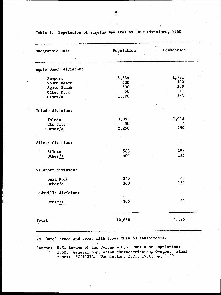
Table 1. Population of Yaquina Bay Area by Unit Divisions, 1960

Geographic unit Population Households

Agate Beach division:

Newport 5,344 1,781

South Beach 300 100

Agate Beach 300 100

Otter Rock 50 17

Other/a 1,600 533

Toledo division:

Toledo 3,053 1,018Elk City 50 17

Other)a 2,250 750

Siletz division:

Siletz 583 194

Other la 400 133

Waldport division:

Seal Rock 240 80

Other/a 360 120

Eddyville division:

Other) 100 33

Total 14,630 4,876

la Rural areas and towns with fewer than 50 inhabitants.Source: U.S. Bureau of the Census - U.S. Census of Population:

1960. General population characteristics, Oregon. Finalreport, PC(1)39A. Washington, D.C., 1961, pp. 1-20.

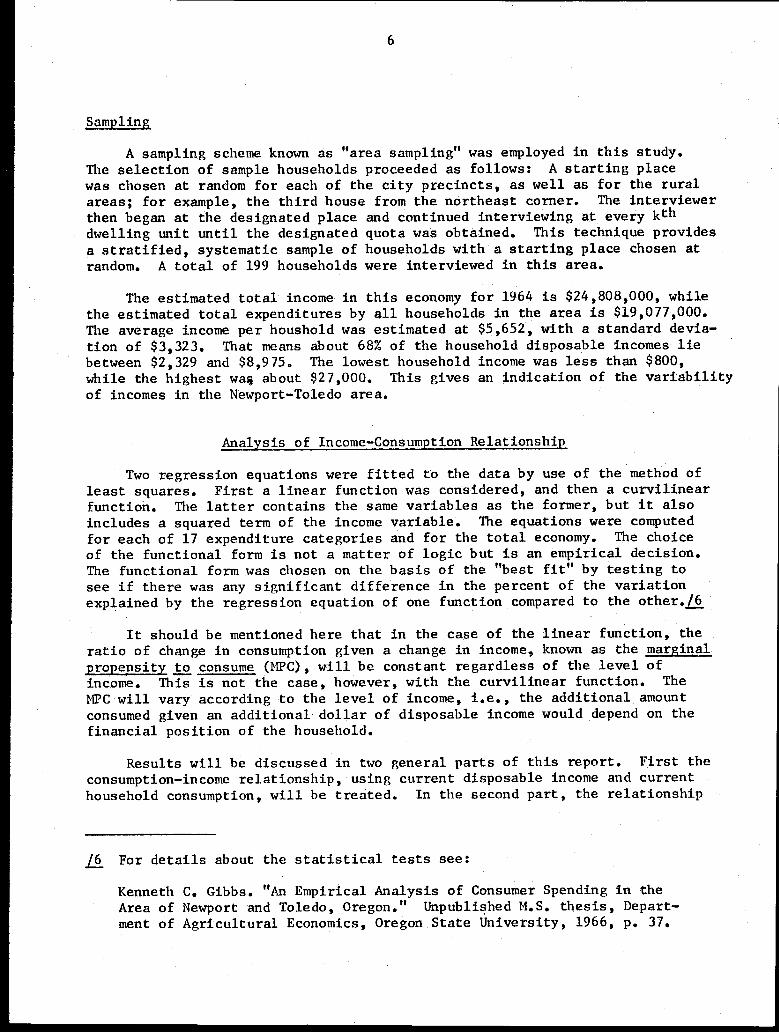
Sampling

A sampling scheme known as "area sampling" was employed in this study.The selection of sample households proceeded as follows: A starting placewas chosen at random for each of the city precincts, as well as for the ruralareas; for example, the third house from the northeast corner. The interviewerthen began at the designated place and continued interviewing at every kthdwelling unit until the designated quota was obtained. This technique providesa stratified, systematic sample of households with a starting place chosen atrandom. A total of 199 households were interviewed in this area.

The estimated total income in this economy for 1964 is $24,808,000, whilethe estimated total expenditures by all households in the area is $19,077,000.The average income per houshold was estimated at $5,652, with a standard devia-tion of $3,323. That means about 68% of the household disposable incomes liebetween $2,329 and $8,975. The lowest household income was less than $800,while the highest was about $27,000. This gives an indication of the variabilityof incomes in the Newport-Toledo area.

Analysis of Income-Consumption Relationship

Two regression equations were fitted to the data by use of the method ofleast squares. First a linear function was considered, and then a curvilinearfunction. The latter contains the same variables as the former, but it alsoincludes a squared term of the income variable. The equations were computedfor each of 17 expenditure categories and for the total economy. The choiceof the functional form is not a matter of logic but is an empirical decision.The functional form was chosen on the basis of the "best fit" by testing tosee if there was any significant difference in the percent of the variationexplained by the regression equation of one function compared to the other./6

It should be mentioned here that in the case of the linear function, theratio of change in consumption given a change in income, known as the marginal propensity to consume (MPC), will be constant regardless of the level ofincome. This is not the case, however, with the curvilinear function. TheMPC will vary according to the level of income, i.e., the additional amountconsumed given an additional dollar of disposable income would depend on thefinancial position of the household.

Results will be discussed in two general parts of this report. First theconsumption-income relationship, using current disposable income and currenthousehold consumption, will be treated. In the second part, the relationship ,

j For details about the statistical tests see:

Kenneth C. Gibbs. "An Empirical Analysis of Consumer Spending in theArea of Newport and Toledo, Oregon." Unpublished M.S. thesis, Depart-ment of Agricultural Economics, Oregon State University, 1966, p. 37.

7

between consumption and income and three additional independent variableswill be discussed.

Consumption as explained by income

The general form of the regression equation in the first part is asfollows:

Ci = a + bY

where: C is the current household consumption in the ith

sector, or expenditurecategory, and Y is the current disposable income of the household, i.e., thegross income of the household less income taxes paid during 1964. The defini-tion of household used in this study is: (1) a group of people usually livingtogether who pool their incomes and draw from a common fund for their majoritems of expense, (2) a person living alone, and (3) a person who isfinancially independent but lives with others, i.e., his income and. expendi-tures are not pooled.

The various sectors of consumption expenditures are enumerated below.

Product-oriented wholesale and retail sector. A few examples of consumptionitems in the product-oriented wholesale and retail sector are groceries,clothing, shoes, home furnishings, flowers, jewelry, electricity, gas, andfeed and seed. The average amount consumed per household for these items was$2,092. The average propensity to consume (APC), i.e., the ratio of consumptionexpenditures to disposable income, at an average income of $5,652, is .37.That is to say, 37% of an average household's income will be spent for goodsand services in this sector./7 The positive relationship between expendituresin this sector and current income does not seem unrealistic. As the level ofincome increases, more furniture, jewelry, shoes, clothing, and the like willbe purchased.

Service-oriented wholesale and retail sector. The service-oriented whole-sale and retail sector includes such consumption items as services from barbershops, beauty shops, laundries and dry cleaners, nonprofit organizations,painters, plumbers, and hospitals. The marginal propensity to. consume is .058,while the average propensity to consume at an average level of income is .066.

/7 The estimated equation pertaining to the product-oriented sector is:

C = $1,015.13 + .19Y

P(.026)

where C is the amount of consumption per household for itemsin the focal product-oriented wholesale and retail firms during1964, and Y is the household disposable income for 1964. Thefigures in parentheses accompanying this and subsequent equationsare the standard errors of the coefficients.

8

The average amount consumed in this sector was $374. Thus, if a householdhad an income of $5,652, it would be expected to consume about 6.6% of itsincome, or $374, for services in this sector.E1

Again, for the service items combined in this expenditure category onewould expect a positive relationship between income and expenditures. Expendi-tures for entertainment and contributions to nonprofit organizations arereadily curtailed at low-income levels and expanded as incomes rise. Theservices of plumbers and painters may be substituted for "do it yourself"labor as incomes rise.

Local government sector. The local government sector includes expendituresfor water and sewage, real estate property taxes, and personal property taxes.The word "consumption" in this context may be misleading. Households makepayments to the local government in the form of taxes for the services itprovides, i.e., for police and fire protection, education, water and sewagedisposal, and so forth. The amount paid to the local government by. householdsis an inadequate measure of the amount of government services consumed by them;however, this amount was used as an approximation of the "consumption" of localgovernment services.

The average amount spent for local government services was $231, with theAPC at an average income of .0441 That is, at an income level of $5,652, ahousehold would be expected to spend approximately 4% of its income for localgovernment services. The MPC is .028; thus, if an additional dollar of dis-posable income were given to a household, on the average about 2.8 cents of itwould be paid to the local government.

Cafes and taverns sector. The cafes and taverns sector consists oflocal consumption in the cafes, restaurants, and bars. The average amountspent in this sector was $218. There was a high degree of variability ofthe amount consumed per household in this expenditure category.

The conclusion reached concerning this sector is that, on the average,a household in the Newport-Toledo area spends about 3.9% of its income in the

/8 The function chosen for this sector is linear, as:

Cs = $48.47 + .058Y

(.0095)where C is the amount of consumption in the service sector by ahousehold in 1964.

/9 The estimated equation for this sector is:

Cg = $74.72 + .028Y(.004)

where C is the amount "consumed" per household in the localgovernment sector.

9

cafes and taverns sector, while if the household had an additional dollaravailable, it would spend approximately another 4 cents in this sector.L10It is interesting to note that among the various expenditure categoriesanalyzed, expenditures in the cafes and taverns sector were the only onesfor which the APC did not exhibit a tendency to decline as incomes rose.

Automotive sector. The average amount spent in this sector was about$619, with a standard deviation of $847. This includes purchases from servicestations, automobile dealers and repair shops, auto supply stores, and motor-cycle sales and service establishments. It was concluded that a positiverelationship exists between current disposable income and household consumption.in this sector. 11

The MPC for this sector is .072 for any level of income. This indicatesthat if, on the average, a household's income went up by one dollar theamount consumed in the automotive sector would increase by 7.2 cents. Sucha relationship can readily be explained. Households with higher incomes arelikely to maintain more automobiles or more expensive ones and are likelyto use them more often than lower-income households. This will result inhigher expenditures for car purchases,. gasoline, repairs, tires, and so forth.

The APC at the average level of income is .11, and will decrease as thelevel of income is increased. Thus, a smaller percent of the disposableincome will be consumed in this sector by the higher than by the lower-incomehouseholds.

It is worth noting that more than 87% of the households in the samplemade expenditures in this sector. There was a relatively wide range inthe amount spent, as can be seen by the high standard deviation.

Communication and transportation sector. Expenditures in this sectorare for such consumption items as newspapers, local trucking, telegrams,television cable, shipping, railroad, and taxis.

/10 The equation that best fits this data is:

Ce = -$25.20 + .043Y

(.017)where C is the dollar value of consumption in the local cafesand taverns in 1964 per household.

/11 The linear function was chosen as:

$.0002 + .0716Yss (.017)

where C is the consumption for goods and services purchasedfrom thSs firms in the automotive sector per household during1964.

10

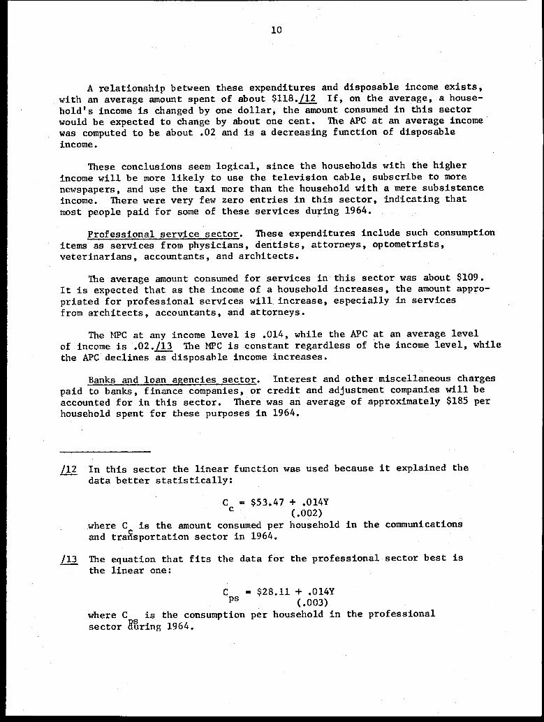
A relationship between these expenditures and disposable income exists,with an average amount spent of about $118411 If, on the average, a house-hold's income is changed by one dollar, the amount consumed in this sectorwould be expected to change by about one cent. The APC at an average incomewas computed to be about .02 and is a decreasing function of disposableincome.

These conclusions seem logical, since the households with the higherincome will be more likely to use the television cable, subscribe to morenewspapers, and use the taxi more than the household with a mere subsistenceincome. There were very few zero entries in this sector, indicating thatmost people paid for some of these services during 1964.

Professional service sector. These expenditures include such consumptionitems as services from physicians, dentists, attorneys, optometrists,veterinarians, accountants, and architects.

The average amount consumed for services in this sector was about $109.It is expected that as the income of a household increases, the amount appro-priated for professional services will. increase, especially in servicesfrom architects, accountants, and attorneys.

The MPC at any income level is .014, while the APC at an average levelof income is .02./13 The MPC is constant regardless of the income level, whilethe APC'declines as disposable income increases.

Banks and loan agencies sector. Interest and other miscellaneous chargespaid to banks, finance companies, or credit and adjustment companies will beaccounted for in this sector. There was an average of approximately $185 perhousehold spent for these purposes in 1964.

In this sector the linear function was used because it explained thedata better statistically:

C = $53.47 + .014Y(.002)

where C is the amount consumed per household in the communicationsand transportation sector in 1964.

/13 The equation that fits the data for the professional sector best isthe linear one:

Cps = $28.11 + .014Y (.003)

where C is the consumption per household in the professionalsector Raring 1964.

11

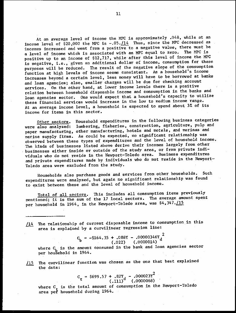
At an average level of income the MPC is approximately .048, while at anincome level of $20,000 the MPC is -.05./14 Thus, since the MPC decreased asincomes increased and went from a positive to a negative value, there must bea level of income which is associated with an MPC equal to zero. The MPC ispositive up to an income of $12,717, while after this level of income the MPCis negative, i.e., given an additional dollar of income, consumption for thesepurposes will be reduced. The result of the negative slope of the consumptionfunction at high levels of income seems consistent. As a household's incomeincreases beyond a certain level, less money will have to be borrowed at banksand loan agencies; also, smaller charges will be due for checking accountservices. On the other hand, at lower income levels there is a positiverelation between household disposable income and consumption in the banks andloan agencies sector. One would expect that a household's capacity to utilizethese financial services would increase in the low to medium income range.At an average income level, a household is expected to spend about 3% of itsincome for items in this sector.

Other sectors. Household expenditures in the following business categorieswere also analyzed: lumbering, fisheries, construction, agriculture, pulp andpaper manufacturing, other manufacturing, hotels and motels, and marinas andmarine supply firms. As could be expected, no significant relationship wasobserved between these types of expenditures and the level of household income.The kinds of businesses listed above derive their incomes largely from otherbusinesses either inside or outside of the study area, or from private indi-viduals'who do not reside in the Newport-Toledo area. Business expendituresand private expenditures made by individuals who do not reside in the NewportToledo area were excluded from the study.

Households also purchase goods and services from other households. Suchexpenditures were analyzed, but again no significant relationship was foundto exist between these and the level of household income.

Total of all sectors. This includes all consumption items previouslymentioned; it is the sum of the 17 local sectors. The average amount spentper household in 1964, in the Newport-Toledo area, was $4,347./15

/14 The relationship of current disposable income to consumption in thisarea is explained by a curvilinear regression line:

Cb = -$164.35 + .088Y - .00000346Yd2

(.022) (.0000014)

where Cb is the amount consumed in the bank and loan agencies sectorper household in 1964.

/15 The curvilinear function was chosen as the one that best explainedthe data:

2C t = $699.57 +

(.where C

t is the total amount of

area per household during 1964.

.82Y - .000023Y111)

d (.0000068)consumption in the Newport-Toledo

12

The APC is .769 for an average income level, i.e., a household with adisposable income of $5,652 would be expected to consume approximately 77%of its income in the Newport-Toledo area. The remaining 23% would eitherbe saved or consumed outside of the area. As the level of income increases,the APC decreases.

The MPC declines as the level of income rises. If an additional dollarof income were made available to a household at the average income level($5,652), one would expect that 56 cents of it would be spent in the studyarea. A higher percentage would be spent locally for income increases atlower income levels. For example, a household receiving an additional, dollarof income when it has only $2,000 available annually for consumption wouldbe expected to spend 73% of it locally. On the other hand, at incomeslarger than $17,826 it is expected that when given an incremental increasein income, a household would actually spend less in this area, but not asmuch less as the increase in income.

It is interesting to speculate about the possible reasons for thenature of this relationship. Two explanations suggest themselves. First,as incomes increase, the marginal propensity to consume goods, regardlessof their place of purchase, may decline. This means that proportionatelylarger amounts of income increases go into savings at higher income levelsthan at lower income levels. Given the use of cross-sectional data in thestudy, this explanation does not seem unreasonable.

Another reason for the curvilinear relationship in this consumptionfunction may be found in the definition of the consumption variable. As willbe recalled, the latter reflects only consumption expenditures made in theNewport-Toledo area. It may be that as incomes rise, a greater proportion ofconsumption expenditures is made outside the local area. Goods and serviceswhich are not available locally may be relatively more important in thehouseholds with larger budgets than in those with smaller ones. Expendituresfor higher education may be an example of this. It may also be possible thathouseholds with relatively high incomes exercise a preference for shoppingin retail markets which are larger than those available in the study area.

Two warnings should be issued at this point about the interpretationof these consumption function results. First, few observations of householdincomes higher than $17,000 were made; thus, not much reliability should beplaced on the consumption-income relationship past this point. Second, theimplications of the cross-sectional consumption function are crucial formaking certain predictions about consumer behavior. Cross-sectional analysisinvolves the observation of consumer spending patterns carried out by house-holds at different income levels. It may be argued that the estimatedfunctional relationship is a good indicator of the change in behavior ofone income group as its financial position changes to that of another incomegroup. Cross-sectional data are an inadequate basis, however, for makingpredictions about consumer behavior when overall changes in incomes occurwhich leave a household's relative income unchanged.

The empirical results presented up to this point are summarized in Table

13

Table 2. Consurptien by Sector, Marginal Propensity to Consume, AveragePropensity to Consume, and Form of Consumption Function(Newport-Toledo Households, 1964)

Additionalamountconsumedgiven anadditional Percent of

Average dollar of income FunctionalSector amount spentLa income (MPC)/11 consumed (APC)a.) form

Product Linear2,092 19.0 37.0

Service 374 5.8 6.6 Linear

Lumber No relation

Government 231 2.8 4.1 Linear

Hotel, motel No relation

Cafes & taverns 218 4.3 3.9 Linear

Marinas & supply -- No relation

Fisheries -- No relation

Automotive 619 7.2 11.0 Linear

Communication 118 1.4 2.1 Linear

Professional 109 1.4 1.9 Linear

Banks & loan 185 4.8 3.3 Curvilinear

Construction -- No relation

Agriculture -- No relation

Households No relation

Pulp & paper -- No relation

All other mfg. -- No relation

Total local 4,347 56.03 76.9 Curvilinear,

La Includes expenditures in those categories only in which the average amountspent was sufficiently large for the relationship with income to be signifi-cant.

DI Computed at an average income of $5,652.

x1

Number living in thehousehold during 1964

3.58(1.77)

x2Number of full-time wage .90earners in the household (.56)in 1964

Age of the head of thehousehold in 1964

Current disposable incomeper household in 1964

42(18)

$5,652($3,323)

x3

x4

14

Consumption as explained by income and other variables

In the theories of consumer behavior, income is singled out in one formor another as the most important variable in explaining consumption. Allother factors are "held constant." Some of these "other factors" are nowconsidered as independent variables (Table 3).

Table 3. Independent Variables Used, Their Means and Standard Deviations

(Newport-Toledo Households, 1964)

Average value of variableSymbol

Variable (Standard deviation of variable)

Each sector was analyzed separately and in each case the independentvariables were chosen as the ones thought to have a relationship withconsumption in that particular sector. The regression equations were computedusing those variables thought to be relevant.

In some of the sectors the independent variables were entered as squaredterms, merely indicating that the relationship was curvilinear rather thanlinear. The statistical procedure used previously was employed here to deter-mine which functional form fit the data best.

The following discussion is devoted to the variables chosen on a sectorby sector basis and to the conclusions drawn about those sectors which utilizedvariables different from those used in the first method. The average amountconsumed in each sector was the same as in the method discussed previously.

15

Product-oriented wholesale and retail sector. The two independent vari-ables chosen in this sector were X 1 , the number in the household, and X4, 4'current disposable income./16

Their relation can readily be justified. As the size of the familyincreases, more money will be spent for food, clothing, shoes, and other house-hold items; thus, a positive relationship exists between X1 and, consumptionin this sector. The relationship of disposable income to consumption in theproduct-oriented sector has already been established.

If the size of a household is held constant and the income were increased.by one dollar, the household would be expected to consume approximately11.9 cents additional in this sector. On the other hand, if the income levelis held constant while the number in the household is increased by one, it isexpected that an additional $275 will be consumed in this sector.

Service-oriented wholesale and retail sector. The same independentvariables that were assumed to be significant in the products sector werechosen in this sector, for similar reasons./17

In this case, the relationship is linear with respect to the level ofincome but curvilinear with respect to the size of the household. If thesize of the household is held constant and the level of income is increasedby one dollar, then an additional 4.6 cents will be consumed in this sector.If, on the other hand, the level of income is held constant and the size ofthe household is changed from two to three, then an additional $18 will beconsumed in this sector. The curvilinear relationship between householdsize and expenditures in this category indicates that larger additions toconsumption for a unit-increase in household size are made in large householdsthan in small ones.

Automotive sector. Disposable income and the number of full-time wageearners were chosen as the independent variables in this sector. If thenumber of wage earners increased, increased expenditures for commuting towork probably would be reflected as consumption in this sector. If, on theaverage, the level of income is held constant and the number of full-time

/16 The regression equation is:

C = $343.96 + 274.66X 1 + .119X

4(46.585) (.021)

where C is consumption in the product-oriented sector.

/17 The data from the sample support this hypothesis. The equation is:

Cs = $1.34 + 3.62X 2 + .046X4

(1.745)1(.006)

where Cs is the amount consumed in the service sector per household.

16

wage earners increases by one, then an additional $236 would be consumedin this sector. /18

Professional services sector. The main expense items in this sector arefor services provided by physicians and dentists; thus, it was thought thatthe level of income, the size of the household, and the age of the householdhead were appropriate independent variables. It should be noted that the agevariable, X3, was not found to be significant./19 This can be attributed, inpart at least, to the fairly high correlation between the variables X1 and X3.

When X1 is entered into the solution, most of the variation is explained, i.e.,

X accounts for very little additional unexplained variation.3

If the level of income is held constant and the size of the householdis allowed to vary by one person, then it is expected that consumption in thissector will change on the average, by $15.

Total of all sectors. Two independent variables were chosen as relevantfor consumption in the Newport-Toledo area: household size and disposableincome.

If the level of income were held constant and the size of the householdincreased from two to three, an additional $204 would be expected to be con-sumed in this area per household, while if the size changed from four to five,$368 additional could be expected to be consumed. 20 Thus, total local con-sumption is a function, increasing at an increasing rate, of the householdsize. If the size of the household were fixed and the level of incomeincreased from $2,000 to $3,000, then, on the average, an additional $502could be expected to be consumed in the area. If, however, the income levelchanged from $10,000 to $11,000, one could expect only $310 more to beconsumed in this area. That is to say that total local consumption is afunction, increasing at a decreasing rate, of disposable income.

/18 The following equation was estimated:

C = $143.01 + 236.25X 2 + .041X4ss (114.54) (.016)

where Css is consumption in the automotive sector per household.

/19 The equation that exhibits the relationship of these items is:

C = -$5.01 + 15.04X1 + .00937X

ps (5.550) (.00025) 4where Cps is consumption in the professional services sector.

/20 The computed equation is:

C t = $726.79 + 40.89X,2 + .562X - .000012X4

2

(10.184T (.09247 (.000004g)where C t

is the total amount consumed in the Newport-Toledoarea per household.

17

SUMMARY

This study had a two-fold objective: (1) to determine the relationshipbetween income and consumption for the Newport-Toledo economy, and (2) todetermine the relationship between consumption and other independent variables,in addition to income. The economy of this area was segregated into 17 expendi-ture categories. A sample of households was chosen, and each one was personallyinterviewed to determine its income and the corresponding amount of consumptionin each of the expenditure categories for the year \of 1964.

The results of this analysis fall into two main categories. The firstdeals with the consumption-income relationship. This method had two variables:current disposable income was the independent variable, and current annualexpenditures for 1964 the dependent variable.

The equation computed for the total local consumption was:

Ct = $699.57 + .82Yd

- .000023Yd2

where C is the total local consumption per household and Y d is the currentdisposable income of the household. The average level of income in this area

'was approximately $5,652, which projects an estimated total income in theeconomy of $24,808,000. The average amount spent per household in 1964 was$4,347; there was an estimated total expenditure in the Newport-Toledo areaof $19,077,000. The previous figures indicate that about 77% of the incomeof the total area was spent within the area.

The second category in which the results were classified is the relation-ship between consumption and three additional independent variables. Thedependent variable was current annual expenditures for 1964. The independentvariables were chosen, from a list of four, for each sector individually. Thefour possible variables were: the size of the household; the number of full-time wage earners; the age of the household head; and current disposableincome. Four sectors, namely product, service, automotive, and professional,were found to exhibit a relation significantly different from that when dispos-able income was the only explanatory variable. The equation derived for totallocal consumption was:

Ct = $726.79 + 40.98X + .562X4 - .000012X

212

4 4

where X4 is current disposable income, X 1

is the size of the household, and

Ct is the total local consumption per household. Total local consumption

is a function, increasing at an increasing rate, of household size. On theother hand, however, total local consumption is a function, increasing ata decreasing rate, of disposable income.