Construction of Minimal Gauge Invariant Subsets of Feynman ... · Construction of Minimal Gauge...

Construction of Minimal Gauge InvariantSubsets of Feynman Diagrams with Loops

in Gauge Theories

Vom Fachbereich Physikder Technischen Universitat Darmstadt

zur Erlangung des Gradeseines Doktors der Naturwissenschaften

(Dr. rer. nat)

genehmigte Dissertation vonDipl.-Phys. David Ondreka

aus Hanau

Referent: Prof. Dr. P. ManakosKorreferent: Prof. Dr. J. Wambach

Tag der Einreichung: 12. 4. 2005Tag der Prufung: 6. 6. 2005

Darmstadt 2005D17

Zusammenfassung

Diese Arbeit beschaftigt sich mit Feynmandiagrammen mit Schleifen in re-normierbaren Eichtheorien mit oder ohne spontane Symmetriebrechung. Es wirdgezeigt, dass die Menge der Feynmandiagramme, die zur Entwicklung einer zu-sammenhangenden Green’schen Funktion in einer bestimmten Schleifenordnungbeitragen, mit Hilfe von graphischen Manipulationen an Feynmandiagrammen,sogenannten Eichflipps, in minimal eichinvariante Untermengen zerlegt werdenkann. Zu diesem Zweck werden die Slavnov-Taylor-Identitaten fur die Entwick-lung der Green’schen Funktionen in Schleifenordnung so zerlegt, dass sie furUntermengen der Menge aller Feynmandiagramme definiert werden konnen. Eswird dann mit diagrammatischen Methoden bewiesen, dass die mittels Eich-flipps konstruierten Untermengen tatsachlich minimal eichinvariante Untermen-gen sind. Anschließend werden die Eichflipps benutzt, um die minimal eichin-varianten Untermengen von Feynmandiagrammen mit Schleifen im Standard-modell zu klassifizieren. Es wird ein ausfuhrliches Beispiel diskutiert und mitResultaten verglichen, die mit Hilfe eines fur die vorliegende Arbeit entwickeltenComputerprogramms erhalten wurden.

Abstract

In this work, we consider Feynman diagrams with loops in renormalizablegauge theories with and without spontaneous symmetry breaking. We demon-strate that the set of Feynman diagrams with a fixed number of loops, con-tributing to the expansion of a connected Green’s function in a fixed order ofperturbation theory, can be partitioned into minimal gauge invariant subsets bymeans of a set of graphical manipulations of Feynman diagrams, called gaugeflips. To this end, we decompose the Slavnov-Taylor identities for the expansionof the Green’s function in such a way that these identities can be defined forsubsets of the set of all Feynman diagrams. We then prove, using diagram-matical methods, that the subsets constructed by means of gauge flips reallyconstitute minimal gauge invariant subsets. Thereafter, we employ gauge flipsin a classification of the minimal gauge invariant subsets of Feynman diagramswith loops in the Standard Model. We discuss in detail an explicit example,comparing it to the results of a computer program which has been developed inthe context of the present work.

i

Contents

1 Introduction 11.1 Overview . . . . . . . . . . . . . . . . . . . . . . . . . . . . . . 5

2 Identities in Gauge Theories 62.1 From Classical Lagrangian to BRST Invariance . . . . . . . . . 62.2 Quantum BRST Transformations and Slavnov-Taylor Identities 9

2.2.1 STI in Unbroken Gauge Theories . . . . . . . . . . . . . 142.2.2 STI in Spontaneously Broken Gauge Theories . . . . . . 15

2.3 Graphical Representation of STIs . . . . . . . . . . . . . . . . . 172.4 STI for Ghost Green’s Functions . . . . . . . . . . . . . . . . . 212.5 Perturbative Expansion . . . . . . . . . . . . . . . . . . . . . . 22

3 Tree Level STIs and Gauge Flips 243.1 STIs and Effective BRST Vertices . . . . . . . . . . . . . . . . 24

3.1.1 Propagator and Inverse Propagator STIs . . . . . . . . . 253.1.2 Cubic Vertices . . . . . . . . . . . . . . . . . . . . . . . 253.1.3 Quartic Vertices . . . . . . . . . . . . . . . . . . . . . . 263.1.4 Five-Point Vertices . . . . . . . . . . . . . . . . . . . . 27

3.2 STIs of Connected Green’s Functions: Examples . . . . . . . . . 283.2.1 The STI for the Connected Three-Point Function . . . . 283.2.2 The STI for the Connected Four-Point Function . . . . 29

3.3 Diagrammatical Relations . . . . . . . . . . . . . . . . . . . . . 313.3.1 Sums and Sets . . . . . . . . . . . . . . . . . . . . . . . 313.3.2 Contraction as Map . . . . . . . . . . . . . . . . . . . . 333.3.3 Decomposing the Contraction Map Θ . . . . . . . . . . . 37

3.4 The STI for the Two-Ghost Four-Point Function . . . . . . . . 393.5 Gauge Cancellations and Gauge Flips . . . . . . . . . . . . . . 413.6 Projections . . . . . . . . . . . . . . . . . . . . . . . . . . . . . 43

4 Groves of General Connected Green’s Functions 444.1 Preliminaries . . . . . . . . . . . . . . . . . . . . . . . . . . . 444.2 STI at One-Loop . . . . . . . . . . . . . . . . . . . . . . . . . 45

4.2.1 Production of Contact Terms . . . . . . . . . . . . . . . 454.2.2 Cancellations in B4(G) . . . . . . . . . . . . . . . . . . 464.2.3 Cancellations in B5(G) . . . . . . . . . . . . . . . . . . 524.2.4 Cancellations in Bc(G) . . . . . . . . . . . . . . . . . . 54

4.3 Groves and Gauge Flips . . . . . . . . . . . . . . . . . . . . . . 584.3.1 Constructing Groves . . . . . . . . . . . . . . . . . . . . 59

4.4 STI at n-loop . . . . . . . . . . . . . . . . . . . . . . . . . . . 64

iii

4.4.1 Production of Contact Terms . . . . . . . . . . . . . . . 644.4.2 Cancellations in B4(G) and B5(G) . . . . . . . . . . . . 674.4.3 Cancellations in Bc(G) . . . . . . . . . . . . . . . . . . 694.4.4 Groves and Gauge Flips . . . . . . . . . . . . . . . . . . 72

5 Unflavored Flips 745.1 Flips Without Flavor: The Basic Tool . . . . . . . . . . . . . . 74

5.1.1 Forest and Flips in Unflavored φ-Theory . . . . . . . . . 755.1.2 Forest and Flips for Higher Order Processes . . . . . . . 775.1.3 1PI Diagrams . . . . . . . . . . . . . . . . . . . . . . . 815.1.4 Amputated Diagrams . . . . . . . . . . . . . . . . . . . 845.1.5 An Explicit Example . . . . . . . . . . . . . . . . . . . 86

6 Flips and Groves in Gauge Theories 926.1 Flips in Gauge Theories . . . . . . . . . . . . . . . . . . . . . . 926.2 Gauge Flips in QCD . . . . . . . . . . . . . . . . . . . . . . . 936.3 Gauge Flips and Groves in the Standard Model . . . . . . . . . 95

6.3.1 Gauge Flips . . . . . . . . . . . . . . . . . . . . . . . . 966.3.2 Gauge Motions . . . . . . . . . . . . . . . . . . . . . . 996.3.3 Pure Boson Forests . . . . . . . . . . . . . . . . . . . . 1046.3.4 General SM Forests . . . . . . . . . . . . . . . . . . . . 1096.3.5 Structure of SM Forests: An Explicit Example . . . . . . 1216.3.6 Generalization . . . . . . . . . . . . . . . . . . . . . . . 1326.3.7 Results . . . . . . . . . . . . . . . . . . . . . . . . . . . 132

7 Summary 136

A BRST Feynman Rules 138A.1 Unbroken Gauge Theories . . . . . . . . . . . . . . . . . . . . . 138

A.1.1 BRST Vertices . . . . . . . . . . . . . . . . . . . . . . . 138A.1.2 Inhomogeneous Parts . . . . . . . . . . . . . . . . . . . 139

A.2 Spontaneously Broken Gauge Theories . . . . . . . . . . . . . . 139A.2.1 BRST Vertices . . . . . . . . . . . . . . . . . . . . . . . 140A.2.2 Inhomogeneous Parts . . . . . . . . . . . . . . . . . . . 140

B Tree Level STIs 142B.1 Propagator and Inverse Propagator STIs . . . . . . . . . . . . . 142B.2 Vertex STIs . . . . . . . . . . . . . . . . . . . . . . . . . . . . 142

B.2.1 Cubic Vertices . . . . . . . . . . . . . . . . . . . . . . . 142B.2.2 Quartic Vertices . . . . . . . . . . . . . . . . . . . . . . 143B.2.3 Five-Point Vertices . . . . . . . . . . . . . . . . . . . . 143

C Automated Grove Construction 144C.1 Implementation . . . . . . . . . . . . . . . . . . . . . . . . . . 144

C.1.1 Representing Feynman Diagrams . . . . . . . . . . . . . 144C.1.2 Comparing Feynman Diagrams . . . . . . . . . . . . . . 145C.1.3 Constructing Groves . . . . . . . . . . . . . . . . . . . . 145

C.2 Usage . . . . . . . . . . . . . . . . . . . . . . . . . . . . . . . 146

iv

—1—Introduction

Over the past decades, the Standard Model has provided us with a remarkablyaccurate description of all experiments within the reach of currently availableexperiments. To challenge the Standard Model, we have to either perform ex-periments at higher energy scales, or else look for deviations from StandardModel predictions in high precision measurements.

In the former case, the processes observed at future high energy colliders(LHC, TESLA) will involve increasingly complicated final states. In particular,at LHC, calculations for processes with eight or more particles in the final statewill have to be performed. In the latter case, increasingly accurate predictionsfrom theory will be required to compare with the experimental results. Thiswill necessitate routine calculations of higher order corrections in the StandardModel.

Despite the indisputable successes of the Standard Model, calculations ofprocesses with many particles in the final state as well as calculations of a fullset of higher order corrections are still inherently difficult. In particular, untilnow there is no tool available for doing fully automated calculations of fullone-loop or two-loop corrections to Standard Model processes.

The reason for this situation is twofold. On the one hand, even at one-loop, the calculation of the contributions of higher tensor n-point functions isextraordinarily difficult, numerically or analytically, through the presence ofmany different masses and the intricate structure of many particle phase space.On the other hand, the number of Feynman diagrams increases dramatically(roughly, the growth is factorial) with the number of loops and the number ofparticles in the final state.

If we aim at a fully automated calculation of higher order corrections inthe Standard Model, progress has to be made in both respects. In this work,we will not be concerned with the problem of actually calculating higher orderdiagrams. Rather, we shall focus on the question whether it is possible to reducethe number of Feynman diagrams necessary to obtain sensible partial results.

One way to avoid the factorial growth of individual contributions to theamplitude is to dispense completely with the definition of the amplitude interms of Feynman diagrams. In QCD calculations, a possible approach is toexpress the amplitude in terms of subamplitudes corresponding to color SU(3)invariants.[1] The contributions of a single invariant will in general be given bya sum of fewer terms than the complete amplitude. However, such an approachis not possible in a gauge theory with spontaneous symmetry breaking, since itmakes use of the linear realization of the color SU(3) symmetry.

1

A second approach, particularly suited to calculations in spontaneously bro-ken gauge theories, is motivated by the observation that in a typical set ofFeynman diagrams there are always subsets of diagrams that have large partsin common. If one can find a systematic way to exploit this feature, the com-plexity of the problem can be considerably reduced. Indeed, an algorithm formatrix element generation based on this approach has been developed [2], whichreduces the combinatorial complexity from a factorial of the number of externalparticles to an exponential. A related earlier algorithm satisfying these require-ments is [3]. However, at present these algorithms are limited to the lowestorder of perturbation theory.

For the calculation of higher order corrections, we still need the contribu-tion of the full set of Feynman diagrams to compute the complete amplitude.However, a major problem in gauge theories like the Standard Model is that thenumerical contribution of an individual diagram to the amplitude may be con-siderably larger, under certain conditions even by several orders of magnitude,than the sum of all diagrams. This can lead to serious numerical problems.In gauge theories, it is therefore desirable to partition the set of all Feynmandiagrams into subsets, such that all the large cancellations dictated by gaugeinvariance would occur separately within each subset.

In fact, few Standard Model calculations of complete higher order correctionsto scattering processes with four or more particles in the final state exist. In mostcases, approximations based on estimation and evaluation of the numericallymost important corrections are used. In general then, only a subset of the fullhigher order corrections is taken into account. Doing this naively may leadto incorrect results due to violation of gauge invariance. In particular, gaugeinvariance in principle dictates the selection of other diagrams once a certainsubset of the complete set of diagrams has been selected, so as to render theresulting expressions gauge invariant.

Of course, by consistently working in a particular gauge, it is actually pos-sible to do calculations with a subset of Feynman diagrams which is not gaugeinvariant by itself, if the contributions of the omitted diagrams are negligible inthe chosen gauge. However, in order to make sure that the omitted diagramscan safely be disregarded, one still has to determine the full set of diagrams thatwould lead to a gauge invariant final result.

It is then natural to ask whether in a gauge theory, spontaneously brokenor not, the set of Feynman diagrams contributing to a given process can bedivided into subsets that lead to gauge invariant expressions by themselves.In this work, we derive and implement an algorithm for the construction ofminimal gauge invariant subsets of Feynman diagrams with loops in generalgauge theories. The algorithm is based on a set of graphical manipulations ofFeynman diagrams, called gauge flips, originally invented for the constructionof minimal gauge invariant subsets of tree diagrams.[4]

Gauge flips are defined as the transformations in four-point subdiagramswith external gauge boson lines.1 As a specific example, consider the transfor-

1In spontaneously broken gauge theories, there are also gauge flips of five-point subdia-grams. For simplicity, we ignore these in the present chapter.

2

mations among the following sets of subdiagrams in the Standard Model:2 , ,

(1.1)

,

(1.2)

Here, wavy lines represent the neutral bosons, i. e. Z0 and photon, while arroweddouble lines denote the charged W bosons.

Although gauge flips have been invented for tree level diagrams, they can bereadily extended to diagrams with loops. As an example, consider the followingdiagram contributing to the process e+e− → uudd at the one-loop level:

e+

e−

d

d

u

u

(1.3)

If we choose to flip the subdiagram defined by the four W -lines connected bythe neutral gauge boson line, we can apply the gauge flips in (1.1) to obtain:

(1.3) →

e+

e−

d

d

u

u

,

e+

e−

d

d

u

u

(1.4)Observe that the flip has decreased the number of vertices in the loop.

We can also increase the number of vertices in the loop. To this end, in (1.3)consider the subdiagram defined by the electron line. This subdiagram can be

2The complete set of Standard Model gauge flips is discussed in chapter 6.

3

flipped using (1.2):

(1.3) →

e+

e−

d

d

u

u

(1.5)

By repeatedly applying similar gauge flips to the resulting diagram, we canincrease the number of vertices in the loop further, producing diagrams withfive or six vertices in the loop:

(1.5) →

e+

e−

d

d

u

u

→

e+

e−

d

d

u

u

(1.6)Thus, gauge flips can be used to transform diagrams contributing to e+e− →uudd into each other. However, this may or may not be true for the completeset of diagrams contributing to this process, called the forest. In general, thegauge flips induce a partition of the forest into disjoint subsets called groves.

For tree level processes, the connection between gauge flips and gauge in-variance is made by a theorem, stating that the groves of a tree level forest areprecisely the minimal gauge invariant subsets of the corresponding connectedGreen’s function.[4][5]

Using this theorem, one can set out to classify the groves of tree level Stan-dard Model processes. One finds [6] that, for purely fermionic external stateswith fermions in the dublet representation of SU(2), the finest possible parti-tioning of the forest corresponds to a classification according to the flavors inthe external state, if a charged boson line is present in the diagrams. On theother hand, for diagrams without a charged boson line, the groves constitute,in general, a finer partitioning.

In this work, we extend the stated theorem to the case of diagrams withloops in general gauge theories. Subsequently, we use the method of gauge flipsto classify the forest of n-loop corrections to general Standard Model processes.We find that, for diagrams containing charged boson lines, the finest possiblepartitioning is characterized by the flavors of fermions in the external state andthe number of fermion loops. On the other hand, the diagrams without chargedboson lines generally show a richer structure of groves than in the tree levelcase.

4

1.1 Overview

The remainder of this work is organized as follows. We intend to prove that thegroves obtained by gauge flips correspond to the minimal gauge invariant subsetsof Feynman diagrams corresponding to the expansion of a connected Green’sfunction at n-loop order in a general gauge theory. To this end, we have to verifythat the relevant Slavnov-Taylor-Identities (STIs) for the Green’s functions ofthe gauge theory are satisfied. In order to put these STIs in a context and tointroduce the necessary notation, we briefly review the derivation of STIs forGreen’s functions in a general gauge theory in the next chapter. There, we alsointroduce a graphical notation for the expansion of STIs in perturbation theory.This requires additional Feynman rules compared to the usual Feynman rulesof a gauge theory.

Our proof of the STIs will be performed by using the STIs for tree levelvertices inside diagrams with loops. Therefore, we derive the relevant tree levelSTIs in chapter 3. We demonstrate the use of vertex STIs in the proof of STIsfor connected Green’s functions at tree level, providing the connection to gaugeflips. Also, we develop further tools that will help to simplify the complicatedcombinatorics of gauge cancellations at the n-loop order.

Chapter 4 is then devoted to the actual proof that groves are the minimalgauge invariant subsets of n-loop forests. We begin by studying the gaugecancellations in one-loop diagrams, then extend our arguments to the n-loopcase. We demonstrate that all cancellations occur within the groves of theforest.

In chapter 5, we introduce the concept of flips for diagrams with loops inde-pendent from the connection with gauge invariance.

In chapter 6, the decomposition of Standard Model forests using gauge flipsis discussed in detail. We obtain a very general classification of Standard Modelforests. As an application, we elaborate on the structure of the one-loop forestfor e+e− → uudd, which we have employed for demonstration purposes above.For this example, we present the results we have obtained by means of ourcomputer program implementing the algorithm for the construction of grovesusing gauge flips. We conclude the main part with a summary.

In the appendix, we collect the Feynman rules for the expansion of STIs, thetree level STIs used in chapters 3 and 4, and a brief description of our programfor grove construction.

5

—2—Identities in Gauge Theories

In this chapter we are going to introduce the Slavnov-Taylor identities (STIs) ofconnected and 1PI Green’s functions in gauge theories. It is these identities thatwe shall use later to demonstrate how the expansion of a connected Green’s func-tion in perturbation theory can be decomposed into separately gauge invariantpieces.

The STIs follow directly from the BRST invariance of the quantized gaugetheory. Therefore, we begin our discussion by briefly sketching the derivation ofBRST invariance. We then demonstrate how BRST invariance can be used toderive STIs for the generating functionals of the Green’s functions of the theory.From these identities the STIs for individual Green’s functions follow easily. Weadopt a notation for the graphical representation of STIs, introducing Feynmanrules to write out the perturbative expansions of STIs.

2.1 From Classical Lagrangian to BRST Invariance

We consider a gauge theory with a gauge group G, which in general may be thedirect product of compact simple groups and abelian U(1) factors. However, forease of notation we shall denote the set of generators of G by a single symbolta. These generators satisfy the commutation relations[

ta, tb]

= ifabctc , (2.1)

with fabc the structure constants of the Lie algebra of G, which we may assumeto be completely antisymmetric. If G is not simple, then fabc vanishes unlessall indices belong to a single simple factor of G.

The gauge bosons W aµ are coupled to a set of fermions Ψ and a set of scalars

Φ. Both Ψ and Φ transform under some—in general reducible—representationof G. Without loss of generality the scalars can be chosen real, in which casethe representation matrices Xa are real and antisymmetric:[

Xa, Xb]

= fabcXc (2.2)

In particular, an infinitesimal gauge transformation, parametrized by a space-time dependent parameter ωa, takes the form

Ψ→ Ψ + iωataΨ (2.3)Φ→ Φ− ωaXaΦ . (2.4)

6

Fermions and scalars are coupled to the gauge bosons through the (gauge) co-variant derivatives. For simplicity, we introduce only vector couplings for thefermions. Thus, the covariant derivatives are given, respectively, by

DµΨ = ∂µΨ− igW aµ t

aΨ (2.5)

DµΦ = ∂µΦ + gW aµX

aΦ . (2.6)

Note that, for a non-simple gauge group G, instead of the product gW a wewould have one such term for each factor of G:

gW a →∑

r

grWar (2.7)

This interpretation will be implied in the following.For the covariant derivatives of Ψ and Φ to transform like Ψ and Φ, respec-

tively, under infinitesimal local gauge transformations, the gauge bosons musttransform according to

W aµ →W a

µ +1g∂µω

a − fabcωbW cµ . (2.8)

It follows that the field strenght tensor F aµν of the gauge bosons, defined by the

commutator of covariant derivatives

[Dµ, Dν ] ≡ −igF aµνt

a , (2.9)

transforms homogeneously under local gauge transformations:

F aµν → F a

µν + ωcfcabF bµν (2.10)

From the classical fields W aµ , Ψ and Φ we can construct the classical Lagrangian

Lcl of the gauge theory, invariant under Lorentz transformations as well as thelocal gauge transformations (2.3), (2.4) and (2.8), and containing only renor-malizable interactions:

Lcl = −14F a

µνFaµν + Ψ (i /D −m) Ψ +

12

(DµΦ) (DµΦ)− V (Φ) (2.11)

Here, the scalar potential V (Φ) is a polynomial in the fields Φ of degree at mostfour, which is invariant under gauge transformations.1

As it stands, the classical Lagrangian (2.11) is not suitable for quantizationin the canonical or path integral formulation. In the former case, the obstacleis the occurrence of first class constraints (in Dirac’s terminology [7]), in thelatter case the path integral is ill defined because the weight factor exp (iScl) isconstant along orbits of the local gauge transformation due to the local gaugeinvariance of the classical action Scl.

If a Lorentz covariant quantization is desired, the standard way to obtainan effective Lagrangian suitable for quantization is the Faddeev-Popov proce-dure [8]. In effect, it amounts to the addition of a gauge fixing Lagrangian Lgf

as well as a ghost Lagrangian Lgh to Lcl:

Lgf = − 12ξa

(Ga[ϕ])2 (2.12)

1Note that we have omitted Yukawa couplings of scalars to fermions. In principle, thesecould be incorporated, but in order to do so we would have to make further assumptions aboutthe representations ta and Xa.

7

Lgh = −ca δGa[ϕω]δωb

cb (2.13)

The gauge fixing functional Ga[ϕ] depends on the gauge fields W aµ and Φ, here

denoted collectively by ϕ. ϕω denotes the gauge transformed fields. For theformalism to be consistent, Ga must not be invariant under local gauge trans-formations. The gauge parameters ξa are arbitrary positive real numbers. ca

and ca are the Faddeev-Popov ghost fields, two multiplets of real, anticommut-ing scalar fields in the adjoint representation.

Given the infinitesimal form of the local gauge transformations (2.8) and (2.4),the functional derivative of the gauge fixing functional Ga can be expressed as

δGa[ϕω]δωb

=δGa

δϕ

δϕω

δωb=δGa

δW bµ

(∂µ − gfabcW c

µ

)− δGa

δΦj(XaΦ)j . (2.14)

In unbroken gauge theories, the gauge fixing function is usually chosen indepen-dent of the scalar fields. The situation is different in spontaneously broken gaugetheories. Here, the gauge fixing function is usually chosen to depend on boththe gauge fields and the scalar fields, at least if the Lagrangian is used to deriveFeynman rules for doing actual calculations in perturbation theory. We willcome back to this point later when we discuss gauge theories with spontaneoussymmetry breaking in a little more detail in a separate section.

Adding Lgf and Lgh to the classical Lagrangian, we get an effective La-grangian suitable for quantization via the path integral approach:

L = Lcl + Lgf + Lgh

= −14F a

µνFaµν + Ψ (i /D −m) Ψ +

12

(DµΦ) (DµΦ)− V (Φ)

− 12ξa

(Ga[ϕ])2 − ca δGa[ϕω]δωb

cb (2.15)

Remarkably, this Lagrangian, though no longer invariant under local gaugetransformations, is invariant under a set of global nonlinear transformationsof the fields, called BRST transformations.[9][10] Under these transformations,a general field ϕ (now including fermion fields) undergoes the change

ϕ→ ϕ+ δϕ , (2.16)

where δϕ is written asδϕ = λsϕ , (2.17)

with λ an infinitesimal Grassmann number. Explicitely, the BRST transforma-tions are given by

sW aµ = ∂µc

a − gfabccbW cµ (2.18a)

sΦ = −gcaXaΦ (2.18b)sΨ = igcataΨ (2.18c)sΨ = −igcaΨta (2.18d)

sca = −12gfabccbcc (2.18e)

sca = − 1ξaGa (2.18f)

8

For the fields W aµ , Ψ and Φ, present in the classical Lagrangian, the BRST

transformation is just a local gauge transformation parametrized by the ghostfield ca (or, rather, by the commuting quantity λca). Therefore, the invariance ofthe classical Lagrangian under BRST transformations is evident. The invarianceof the gauge fixing and ghost terms can be shown using the Jacobi identity forthe structure constants fabc.

Although the effective Lagrangian (2.15) in connection with the BRST in-variance is sufficient for a consistent covariant quantization of the gauge theoryvia the path integral approach, the BRST invariance can best be exploited byrecasting (2.15) into a slightly different form through the introduction of theNakanishi-Lautrup auxiliary field Ba.[11][12] To this end, instead of the gaugefixing Lagrangian (2.12) one chooses the Lagrangian

LNL =ξa

2BaBa +BaGa . (2.19)

The equation of motion for Ba following from this Lagrangian is

0 = ξaBa +Ga . (2.20)

Thus, Ba has no independent dynamics. (This justifies the term “auxiliary”field.) Solving for Ba and inserting back into (2.19), we get back to the originalgauge fixing Lagrangian (2.12). Also, through this equation of motion, theBRST transformations (2.18f) and (2.21) are equivalent.

The advantage of choosing LNL instead of Lgf is that the BRST transfor-mation s is now nilpotent also off-shell, provided we modify the BRST trans-formation properties according to

sca = Ba (2.21)sBa = 0 . (2.22)

The BRST invariance of the modified Lagrangian

L′ = Lcl + LNL + Lgh (2.23)

follows easily from the nilpotency of the BRST operator s and the observationthat the gauge fixing plus ghost Lagrangian can be written as a BRST variation:

LNL + Lgh = s

(ca

(ξa2Ba +Ga

))(2.24)

Thus, since, as argued above, the classical Lagrangian is BRST invariant, so isthe complete Lagrangian L′.

2.2 Quantum BRST Transformations andSlavnov-Taylor Identities

So far, we have discussed the BRST invariance of the effective gauge theoryLagrangian L in (2.15) (or, equivalently, the modified Lagrangian L′ in (2.23))in a purely classical setting.

We must now ask whether the BRST invariance of the classical Lagrangiansurvives the quantization procedure. This question is nontrivial because the

9

BRST transformations are nonlinear in the fields and therefore require renor-malization. Fortunately, the quantized gauge theory is still invariant underrenormalized BRST transformations.

In the operator formulation, i. e. canonical quantization, this means that,provided the theory is free of anomalies, there exists a renormalized BRSToperator Q, which generates the BRST transformation on the state vector spaceof the theory, such that

[iλQ,ϕ] = λsϕ , (2.25)

where ϕ is a generic (renormalized) field operator, and λ a Grassmann valuedparameter.[13][14]

In the path integral formulation, the statement means that the identitiesobtained by naively applying the classical BRST transformations are valid inthe renormalized theory.

The importance of the BRST operator Q for a consistent Lorentz covariantquantization can hardly be overemphasized. In particular, Q can be used toconstruct a physically satisfactory Hilbert Space with a positive definite metric,in which the S-matrix for physical external states can be shown to be unitaryand gauge invariant. In fact, the classification of the asymptotic state vectorspace into physical and unphysical states depends crucially on the existenceof the BRST operator Q. Namely, unphysical states are states |β〉 for whichQ |β〉 6= 0, while physical external states |phys〉 must satisfy Q |phys〉 = 0.In addition, there are states states |α〉 of the form |α〉 = Q |β〉, which satisfyQ |α〉 automatically due to the nilpotency of Q. These states are called BRST-exact. A BRST-exact state is physically equivalent to the null vector. That is,|phys〉+ |α〉 and |phys〉 describe the same physical state.

The BRST transformations of the asymptotic states can be derived fromthe BRST transformations of the asymptotic field operators, using the LSZformalism. Asymptotically, only terms linear in field operators contribute tothe BRST transformations. We split the BRST transformation sϕ of a genericfield into a term linear and quadratic in fields, respectively, according to

sϕ = %ϕ[c] + ca∆aϕ . (2.26)

Here, %ϕ[c] may contain derivatives, while ∆a is just a complex valued matrix.As an example, consider the BRST transformation law (2.18a) of the gaugeboson, where we have %a

W [c] = ∂ca and ∆abcW

c = −gf bacW c.Equivalently, (2.26) is a split into inhomogeneous and homogeneous pieces,

respectively. Using this decomposition, the asymptotic field operator corre-sponding to ϕ generates an unphysical state precisely if %ϕ[c] is nonzero. TheBRST-exact states then are generated by the asymptotic field operators corre-sponding to %ϕ[c].

Given the existence of renormalized BRST transformations, we can derivethe Slavnov-Taylor identities for Green’s functions of the gauge theory. To thisend, we consider the generating functional for the full Green’s functions of thetheory. Due to the necessity to renormalize the nonlinear BRST transforma-tions, we are forced to introduce not only sources J` for the generic field ϕ`,but also sources K` for the BRST transforms sϕ`. Furthermore, if we do notconsider Green’s functions with Ba fields, we can use the Lagrangian L andomit the field Ba everywhere, using (2.18f) as the BRST transformation of theantighost field. We assume that the gauge fixing functional Ga is linear in the

10

fields. Therefore, we need not introduce a source term for the BRST transformof the antighost. Under these assumptions, the generating functional Z[J,K] ofGreen’s functions with insertions of BRST transformed field operators is thengiven explicitely, in path integral formulation, by

Z[J,K] =∫D[ϕ] exp

i

(S +

∑ϕ

Jϕ · ϕ+∑

ϕ 6=ca

Kϕ · sϕ

). (2.27)

In this equation, a dot denotes space time integration. S =∫d4xL is the action

corresponding to the effective Lagrangian L. The sums extend over all fields inL, except that the antighost field can be omitted in the second sum, because ofthe linearity of Ga.

Using the invariance of the path integral measure and the action S underBRST transformations, we obtain the Slavnov-Taylor identities (STIs) for thegenerating functional Z:[15][16]

0 =

∑ϕ 6=ca

(−1)ϕJϕ ·δ

δKϕ+

1ξaGa

[δ

δJ

]Jca

Z[J,K] (2.28)

Here, (−1)ϕ is +1 or −1 for bosonic or fermionic fields, respectively.Defining the generating functional Zc[J,K] of connected Green’s functions

(with insertions of BRST transformed field operators) by

Z[J,K] = exp (iZc[J,K]) , (2.29)

it is easy to see that Zc satisfies an identical STI:

0 =

∑ϕ 6=ca

(−1)ϕJϕ ·δ

δKϕ+

1ξaGa

[δ

δJ

]Jca

Zc[J,K] (2.30)

Connected Green’s functions are obtained from Zc by taking functional deriva-tives2 of Zc w.r.t. the sources Jϕ, putting all sources J and K to zero afterwards.Therefore, the STI (2.30) for Zc implies STIs for individual connected Green’sfunctions.

Now in order to obtain a nonzero Green’s function after setting sources tozero, functional derivatives w.r.t. fermionic sources, i. e. the sources JΨ, JΨ, Jca ,and Jca , must come in pairs. That is, there must be as many derivatives w.r.t. JΨ

and Jca as there are derivatives w.r.t. JΨ and Jca , respectively. However, thefunctional differentiation operator acting on Zc in (2.30) has ghost number one.Therefore, in order to obtain a nonzero STI for an individual connected Green’sfunction, we have to take an additional functional derivative w.r.t. the sourceof the antighost Jca .

In this work, we will be exclusively concerned with the STIs for connectedGreen’s functions with a single insertion of the gauge fixing functional Ga.Therefore, we shall use the term “STI” exclusively in this sense in this work,unless explicitely stated otherwise. In particular, these STIs ensure that a single

2We take all functional derivatives with respect to anticommuting quantities as left deriva-tives.

11

insertion of the unphysical linear combination of fields corresponding to Ga doesnot contribute in matrix elements on the mass shell.

Now consider the functional derivative of (2.30) w.r.t. the source Jcb . Takingcare of fermion signs, we get

0 =

∑ϕ 6=ca

Jϕδ

δJcb

δ

δKϕ− 1ξbGb

[δ

δJ

]+

1ξaGa

[δ

δJ

]Jca

δ

δJcb

Zc[J,K] .

(2.31)Evidently, further functional derivatives w.r.t. Jca will produce further termswith a single insertion of Ga, but no Green’s function with more than oneinsertion of Ga can be produced. Therefore, all STIs for connected Green’sfunctions with a single insertion of the gauge fixing functional Ga are exhaustedby taking arbitrary functional derivatives of (2.30) w.r.t. sources Jϕ.3

In order to determine the explicit form of an STI for a connected Green’sfunction, it is actually easier to work in the canonical formalism. Remember thatin the canonical formalism we have the BRST operator Q which is nilpotent,hermitean, and annihilates the ground state |0〉. Therefore, if φ` are genericfields of the theory, we immediately have4

0 =⟨[

iλQ,ϕ1 . . . ϕn

]⟩c, (2.32)

where here and in the following, the superscript c indicates a connected Green’sfunction. Evaluating the commutator with the help of (2.25), we get

0 =∑

`

〈ϕ1 . . . (λsϕ`) . . . ϕn〉c . (2.33)

Using the decomposition (2.26) of sϕ, this can be rewritten

0 =∑

`

(−1)σ`

(〈ϕ1 . . . %ϕ`

. . . ϕn〉c + 〈ϕ1 . . . (ca∆aϕ`) . . . ϕn〉c). (2.34)

The sign factor counts the number of anticommuting field operators precedingthe `th field.

We can get rid of the sign factor for the second term by moving the ghost ca inthe homogeneous parts to the left. The same can be done for all inhomogeneouspieces in the BRST transformation of bosonic fields, because % is fermionic forthese. On the other hand, the only fermionic field variables with a nonzero %are the antighost fields ca. It is convenient to write

%ca = − 1ξaGa ≡ Ba , (2.35)

using Ba as an abbreviation.5 If we write antighost fields first in connectedGreen’s functions, the generic STI takes the form, with ϕ` now denoting anyfield except antighosts and a caret indicating omission,

3Remember that, if there is no derivative w.r.t. Jϕ, or if derivatives w.r.t. fermion sourcesdon’t come in pairs, the resulting identity is just the trivial statement 0 = 0.

4In this and subsequent equations, we suppress the spacetime arguments of the field oper-ators in Green’s functions. The correct argument should always be clear from the indices.

5Note that we have defined the generating functionals Z and Zc with the action S =Rd4xL, in which Ba does not appear.

12

0 =m∑

k=1

(−1)k+1 〈ca1 . . . Bak . . . camϕ1 . . . ϕn〉c

+∑

`

(〈%ϕ`

ca1 . . . camϕ1 . . . ϕ` . . . ϕn〉c +⟨cbca1 . . . camϕ1 . . . (∆bϕ`) . . . ϕn

⟩c)(2.36)

The signs in the first sum are essential. However, if this sum has more thanone term, we have an STI for a Green’s function with external ghost lines.6

Since ghosts are unphysical degrees of freedom, such Green’s functions are lessfrequently needed, although in unbroken gauge theories, like QCD, ghost am-plitudes may be usefully employed in evaluating gluon polarization sums. Inspontaneously broken gauge theories, like the SM, amplitudes for ghost produc-tion are rarely needed.

In this work—with a single exception, that can easily be treated explicitely—we will not need STIs for Green’s functions with external ghost lines. Therefore,we specialize now to the case of a single antighost field. The resulting STI forconnected Green’s functions is the central identity in this work:

0 = 〈Baϕ1 . . . ϕn〉c

+∑

`

(〈%ϕ`

caϕ1 . . . ϕ` . . . ϕn〉c +⟨cbcaϕ1 . . . (∆bϕ`) . . . ϕn

⟩c)(2.37)

We will later introduce a graphical notation to represent this STI. First, however,we discuss the STIs for the 1PI Green’s functions of the theory. We denoteby Γ[ϕ,K] the generating functional for 1PI Green’s functions with insertionsof BRST transformed operators. Γ[ϕ,K]. Is obtained from Zc by Legendretransformation w.r.t. the sources Jϕ, but not Kϕ:

Γ[ϕ,K] = Zc[J,K]−∑ϕ

Jϕ · ϕ (2.38)

Here, the argument ϕ of Γ is defined as

ϕ = 〈ϕ〉cJ,K =δZc

δJϕ[J,K] . (2.39)

Note that we use the same symbol ϕ for the expectation value as well as for thefield operator. The subscript on the connected Green’s function indicates thatthe Green’s function is to be evaluated in the presence of the external sourcesJ and K. Thus, Γ[ϕ,K] is the effective action in the presence of the externalsources K.

We will generally denote functional derivatives of Γ w.r.t. ϕ or K by sub-scripts. Thus,

δΓδϕ≡ Γϕ (2.40)

δΓδKϕ

≡ ΓKϕ . (2.41)

6Of course, the insertions of BRST transformed operators may lead to Green’s functionswith external ghost fields in the STI. These external ghosts are unavoidable.

13

Γ[ϕ,K] satisfies the fundamental relations

Γϕ[ϕ,K] = −(−1)ϕJϕ (2.42)δΓδKϕ

[ϕ,K] =δZc

δKϕ[J [ϕ],K] . (2.43)

Using (2.42) and (2.43) and the chain rule for functional differentiation, (2.30)can be transformed into an identity for Γ:

0 =∑

ϕ 6=ca

Γϕ · ΓKϕ −1ξaGa[ϕ]Γca (2.44)

This is the STI for the generating functional of 1PI Green’s functions, also calledLee identity.[17][18] The Lee identity implies STIs for individual 1PI Green’sfunctions. Eventually, we will introduce a graphical notation for these identies,too. Before we can do this, however, we must leave our general discussion andconsider the explicit form of the STIs for connected and 1PI Green’s functionsin unbroken and broken gauge theories.

2.2.1 STI in Unbroken Gauge Theories

In unbroken gauge theories, the scalars Φ coupled to the gauge bosons mustnot have vacuum expectation values that would break the invariance under agenerator Xa of the gauge group, i. e. the vacuum expectation value 〈Φ〉 mustsatisfy

Xa 〈Φ〉 = 0 . (2.45)

for all generators Xa, which implies 〈Φ〉 = 0 for all components of Φ thatcouple to at least one gauge boson. But this means that sΦ = 0, which in turnis equivalent to the statement that all scalars are physical fields. In particular,there is no inhomogeneous term in the BRST transformation of the scalars. Thesame applies to the fermion fields Ψ and Ψ.

Consequently, apart from the antighost field, the gauge field W aµ is the only

field with an inhomogeneous term in the BRST transformation law. We choosethe Lorentz covariant linear gauge fixing functional

Ga = ∂µW aµ . (2.46)

Equivalently, we set

Ba = − 1ξa∂µW a

µ . (2.47)

Of course, for doing actual calculations one would choose the ξa equal withina factor of the gauge group G, since this makes the gauge fixing Lagrangianinvariant under global gauge transformations. However, this is only a matter ofconvenience.

We can now write down the explicit form of the STI (2.37) in an unbrokengauge theory:

0 = − 1ξa∂µ⟨W a

µϕ1 . . . ϕn

⟩c+

∑ϕ`=W a

µ

∂µ`〈ca` caϕ1 . . . ϕ` . . . ϕn〉c +

∑ϕ` 6=ca

〈ca` caϕ1 . . . (∆a`ϕ`) . . . ϕn〉c

(2.48)

14

2.2.2 STI in Spontaneously Broken Gauge Theories

In a spontaneously broken gauge theory, the scalar potential V produces anonzero vacuum expectation value (vev) 〈Φ〉 ≡ Φ0, which in general is invariantunder a subgroup H of the full gauge group G. We use greek indices to labelthe generators of broken symmetries and latin indices following q to label thegenerators of unbroken symmetries. Thus, broken and unbroken generatorssatisfy, respectively,

XαΦ0 6= 0 (2.49)XqΦ0 = 0 (2.50)

. (2.51)

According to Goldstone’s theorem,[19][20] before the theory is coupled to thegauge bosons, there is a massless Goldstone boson corresponding to each brokengenerator Xα. Once the set of broken generators has been determined, we canalways arrange Φ in such a way that its first components correspond preciselyto the Goldstone bosons φα. This leads to the following decomposition of Φ:

Φ =(φη

)(2.52)

Correspondingly, the generators Xa of G can be written as block matrices:

Xa =(

ta ua

−(ua)T T a

)(2.53)

Φ0 has no components in the directions of the Goldstone bosons:

Φ0 =(

0v

)with v = 〈η〉 (2.54)

To generate a useful perturbative expansion, the Lagrangian L has to be ex-panded about the vev Φ0. To this end, the scalars η are reparametrized as

η = v +H . (2.55)

We will not carry out the expansion of the Lagrangian, for the results are wellknown. Most importantly, the gauge bosons corresponding to broken generatorsaquire masses through the Higgs mechanism. For our further considerations, wewill need an expression for the gauge boson masses in terms of the brokengenerators Xα and the vev v. First, observe that the broken generators Tα

must satisfyTαv = 0 , (2.56)

because all nonzero vectors of this form point into the direction of Goldstoneboson fields. Next, by choosing the basis in the space of Goldstone bosonsaccordingly, we can always arrange that

uαv ≡ 1gMαe

α , (2.57)

where eα is a unit vector in the Goldstone boson subspace in the direction ofuαv. With these conventions, the mass matrix M2 for the gauge bosons isdiagonal:

M2αβ = g2vT (uα)T

uβv = M2αδαβ . (2.58)

15

On the other hand, from fact that the unbroken generators Xq form a subgroup,it can be shown that these generators are block diagonal, i. e. both φ and Htransform linearly under the subgroup H:

XqΦ = Xq(Φ− Φ0

)=(tqφT qH

)(2.59)

We are now ready to determine the BRST transformation properties of the scalarfields φ and H. The Lagrangian L is invariant under a BRST transformation ofthe original field Φ. Inserting the expansion (2.55), we obtain

sφα = −cαMα − gcβ((tβφ)α + (uβH)α

)− gcq(tqφ)α (2.60a)

sH = −gcα(− (uα)T

φ+ TαH)− gcqT qH . (2.60b)

The inhomogeneous term in the BRST transformation law of φ indicates clearlythat the Goldstone bosons, when coupled to gauge bosons, become unphysicaldegrees of freedom. Therefore, they are often referred to in the literature aswould-be Goldstone bosons or Goldstone ghosts. In this work, we will use theterm “Goldstone boson” exclusively for the unphysical scalar degrees of freedomof a spontaneously broken gauge theory. No confusion is possible, because wedo not consider physical Goldstone bosons of a broken global symmetry.

On the other hand, the fields H, lacking an inhomogeneous term in theirBRST transformation law, form a set of physical scalars, which we refer to asHiggs bosons.7

Like in the case of the unbroken gauge theory, the BRST transformationof the antighost is determined by the gauge fixing functional. For the massivegauge bosons corresponding to broken symmetries, we choose a general linear’t Hooft gauge fixing:[21]

Gα = ∂µWαµ − ξαMαφ

α ≡ −ξαBα (2.61)

This choice is essentially uniquely determined by requiring, in addition to lin-earity in fields and Lorentz covariance, that the Lagrangian contain no bilinearmixing between Goldstone bosons and gauge bosons. Thus, the BRST trans-formation law of the antighost fields cα explicitely reads

scα = − 1ξa∂µWα

µ +Mαφα . (2.62)

For the massless gauge bosons corresponding to unbroken symmetries, we choosethe same gauge fixing (2.46) as in the case of unbroken gauge theories. Likewise,the BRST transformation properties of W a

µ , ca, Ψ and Ψ remain the same. Con-sequently, the explicit form of the STI (2.37), for an antighost cα correspondingto a broken generator, is given by

0 = − 1ξα∂µ⟨Wα

µ ϕ1 . . . ϕn

⟩c +Mα 〈φαϕ1 . . . ϕn〉c

7In general, only some of the components of η will aquire a nonzero vev. In other words,the vector v may contain many zeros. Those components of η with nonzero vevs are the realHiggs bosons, while the remaining components have nothing to do with symmetry breaking.It is, however, not uncommon to use the term “Higgs boson” for all components of H.

16

+∑

ϕ`=W aµ

∂µ`〈ca` cαϕ1 . . . ϕ` . . . ϕn〉c −

∑ϕ`=φα

Mα`〈ca` cαϕ1 . . . ϕ` . . . ϕn〉c

+∑

ϕ` 6=ca

〈ca` cαϕ1 . . . (∆a`ϕ`) . . . ϕn〉c . (2.63)

Observe that, in contrast to the situation in unbroken gauge theories, this iden-tity relates two different Green’s functions for unphysical fields to the sums overGreen’s functions with BRST insertions.

The choice of the ’t Hooft gauge fixing (2.61) has other profound effects: Onone hand, it leads to the gauge parameter dependent masses

√ξαMα for the

scalar modes of a massive gauge boson Wαµ as well as the associated Goldstone

bosons and ghosts φα, cα, and cα, respectively. On the other hand, it intro-duces gauge parameter dependent ghost-scalar interactions. These effects areimportant when studying the gauge parameter dependence of Green’s functions.

2.3 Graphical Representation of STIs

Having discussed in detail the explicit form of the STIs for connected Green’sfunctions in unbroken and broken gauge theories, we are now going to discussa graphical notation to represent these STIs, invented in [5]. We can treatunbroken and broken gauge theories on an equal footing, if we formally defineMq = 0 and φq ≡ 0 for unbroken generatros Xq. The details can always be filledin by going back to the explicit expressions derived in the foregoing section.

An even more compact notation is obtained if we treat gauge bosons andGoldstone bosons as components of a single five dimensional gauge field Aa

r :

Aar =

(W a

µ , φa)

(2.64)

Introduce a five dimensional derivative operator according to

Θar(x) =

(− 1ξa∂x

µ,Ma

)(2.65)

Θar(x) =

(∂x

µ,−Ma

). (2.66)

Employing this notation, the insertion of Ba in a Green’s function can be written

〈Baϕ1 . . . ϕn〉c = Θar 〈Aarϕ1 . . . ϕn〉c . (2.67)

The inhomogeneous terms in the BRST transformation laws of gauge bosonsand Goldstone bosons are given by

sAar

∣∣inhom

= Θarc

a . (2.68)

Then, the STI for connected Green’s functions takes the unified form

0 = Θas 〈Aasϕ1 . . . ϕn〉c +

∑ϕ` 6=ca

〈ca` caϕ1 . . . (∆a`ϕ`) . . . ϕn〉c

+∑

ϕ`=Aar

Θa`r 〈ca` caϕ1 . . . ϕ` . . . ϕn〉c . (2.69)

17

We will represent all fields but ghost and antighosts collectively as straightlines. Ghosts and antighosts, on the other hand,are drawn, as usual, in dottedstyle with arrows indicating ghost number flow. Thus, we have the followingassociations:

Aar ,H,Ψ, Ψ

→ (2.70)

ca, ca → c c (2.71)

We will frequently need a special notation for gauge bosons and Goldstonebosons, which have inhomogeneous terms in their BRST transformation laws.To denote these fields exclusively, we use a wavy line:

Aar → (2.72)

Next we have to represent the BRST transformed operators sϕ. We will useseparate notations for the homogeneous parts and the inhomogeneous parts.The homogeneous parts, present for all fields except antighosts, will be drawnas follows:

ca∆aϕ → (2.73)

The inhomogeneous parts in the transformation of gauge bosons and Goldstonebosons are denoted by

Θarc

a → r. (2.74)

Finally, the insertion of Ba will be represented by a double line:

Ba = ΘarAar → (2.75)

Using these conventions, the STI (2.69) is represented graphically as

0 = +∑

`

`

+∑

`

`

. (2.76)

To complete our conventions for the graphical notation, we note that connectedGreen’s functions will always be denoted by shaded blobs. Next, a dot at theend of an external line indicates that the corresponding line is not amputated.Since we will later deal with 1PI Green’s functions and Green’s functions withamputated external lines, these distinctions are essential. Finally, observe thatwe have deliberately chosen a diamond shaped blob for the connected Green’sfunctions with insertions of ca∆aϕ. This distinction is made because, in pertur-bation theory, most contributions to these Green’s functions are contact terms.This means that, in momentum space, most contributions vanish when all ex-ternal lines are multiplied by inverse propagators and external momenta are setto onshell values.

The case of the two-point function, i. e. the propagator, is special, because inthis case it does not make sense to consider amputation. Therefore, we do notuse a diamond shaped blob in the corresponding STI, which we state explicitely:

0 = + + (2.77)

18

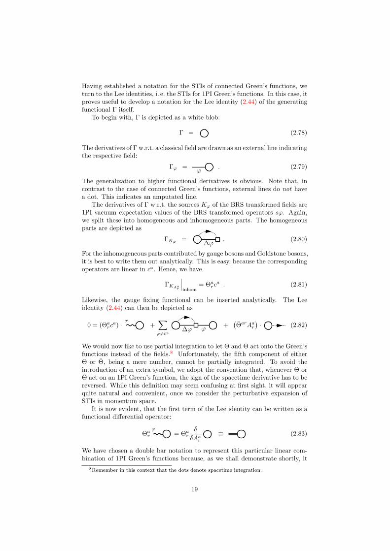
Having established a notation for the STIs of connected Green’s functions, weturn to the Lee identities, i. e. the STIs for 1PI Green’s functions. In this case, itproves useful to develop a notation for the Lee identity (2.44) of the generatingfunctional Γ itself.

To begin with, Γ is depicted as a white blob:

Γ = (2.78)

The derivatives of Γ w.r.t. a classical field are drawn as an external line indicatingthe respective field:

Γϕ =ϕ

. (2.79)

The generalization to higher functional derivatives is obvious. Note that, incontrast to the case of connected Green’s functions, external lines do not havea dot. This indicates an amputated line.

The derivatives of Γ w.r.t. the sources Kϕ of the BRS transformed fields are1PI vacuum expectation values of the BRS transformed operators sϕ. Again,we split these into homogeneous and inhomogeneous parts. The homogeneousparts are depicted as

ΓKϕ=

∆ϕ. (2.80)

For the inhomogeneous parts contributed by gauge bosons and Goldstone bosons,it is best to write them out analytically. This is easy, because the correspondingoperators are linear in ca. Hence, we have

ΓKAar

∣∣∣inhom

= Θarc

a . (2.81)

Likewise, the gauge fixing functional can be inserted analytically. The Leeidentity (2.44) can then be depicted as

0 = (Θarc

a) · r +∑

ϕ 6=ca∆ϕ ϕ

+(ΘarAa

r

)· (2.82)

We would now like to use partial integration to let Θ and Θ act onto the Green’sfunctions instead of the fields.8 Unfortunately, the fifth component of eitherΘ or Θ, being a mere number, cannot be partially integrated. To avoid theintroduction of an extra symbol, we adopt the convention that, whenever Θ orΘ act on an 1PI Green’s function, the sign of the spacetime derivative has to bereversed. While this definition may seem confusing at first sight, it will appearquite natural and convenient, once we consider the perturbative expansion ofSTIs in momentum space.

It is now evident, that the first term of the Lee identity can be written as afunctional differential operator:

Θar

r= Θa

r

δ

δAar

≡ (2.83)

We have chosen a double bar notation to represent this particular linear com-bination of 1PI Green’s functions because, as we shall demonstrate shortly, it

8Remember in this context that the dots denote spacetime integration.

19

is closely related to the insertion of Ba in a connected Green’s function. In asimilar manner, we can represent the last term as

Aar · Θar =

r ·Aar (2.84)

Notice the absence of a dot at the end of the line. This allows a distinctionfrom the symbols used for connected Green’s functions. The change in theorder of factors has been performed to make more apparent, that the spacetimeargument associated with the end of the ghost line is the same as that of Aa

r .The Lee identity for the generating functional of 1PI Green’s functions now

takes the final form

0 = ca × +∑

ϕ 6=ca∆ϕ ϕ

+r ·Aa

r . (2.85)

Some remarks concerning the interpretation of this identity are in order. Mostimportantly, this identity is still dependent on external sources. Therefore, de-spite appearances, ghost number is not violated in the displayed diagrams. Asecond consequence of the source dependence is that individual 1PI Green’sfunctions in the identity are in general not proportional to momentum conserv-ing delta functions in momentum space. Finally, since, in this work, we have noneed for Green’s functions with more than one insertion of a BRST transformedoperator, we will implicitely assume that the sources Kϕ are set to zero.

A further remark concerns the term involving the homogeneous parts of theBRST transformations. We emphasize that the ϕ-line in the homogeneous termis not a propagator. Rather, this term represents the multiplication (or, moreprecisely, convolution) of two 1PI Green’s functions.

In spite of these cautionary remarks, the prescription for deriving STIs forindividual 1PI Green’s functions is actually simple: Take a suitable number offunctional derivatives w.r.t. fields ϕ, remembering to apply the product rule fordifferentiation, and afterwards set sources to zero. In particular, to obtain anonzero identity after setting sources to zero, at least one derivative w.r.t. aghost field ca must be taken.

To illustrate the rules, we derive a master identity for 1PI Green’s funtionswithout external ghost lines. This is done by taking a functional derivativew.r.t. ca and setting ca and ca to zero. The result is:

0 = +∑

ϕ 6=ca,ca∆ϕ ϕ

+r ·Aa

r (2.86)

We will soon need the STI for the inverse propagators with at least one Aar -line,

which we can readily get by taking a functional derivative w.r.t. Aar and setting

all sources to zero:

0 = + + (2.87)

Here and in the following, the sum over fields should be implied. In momentumspace, this is now really an identity among momentum conserving 1PI Green’sfunctions, where the homogeneous term contains the product of two such Green’s

20

functions. The sum is over all bosonic fields that do not carry a conservedquantum number.

Since the Lee identities are nonlinear identities, the product rule would makeit rather cumbersome to depict an STI for an individual 1PI Green’s functionwith several external lines, like we did for the STIs of connected Green’s func-tions in (2.76). Therefore, we refrain from doing so in this general setting. Wewill have ample opportunity to demonstrate the explicit form of such STIs inthe perturbative expansions.

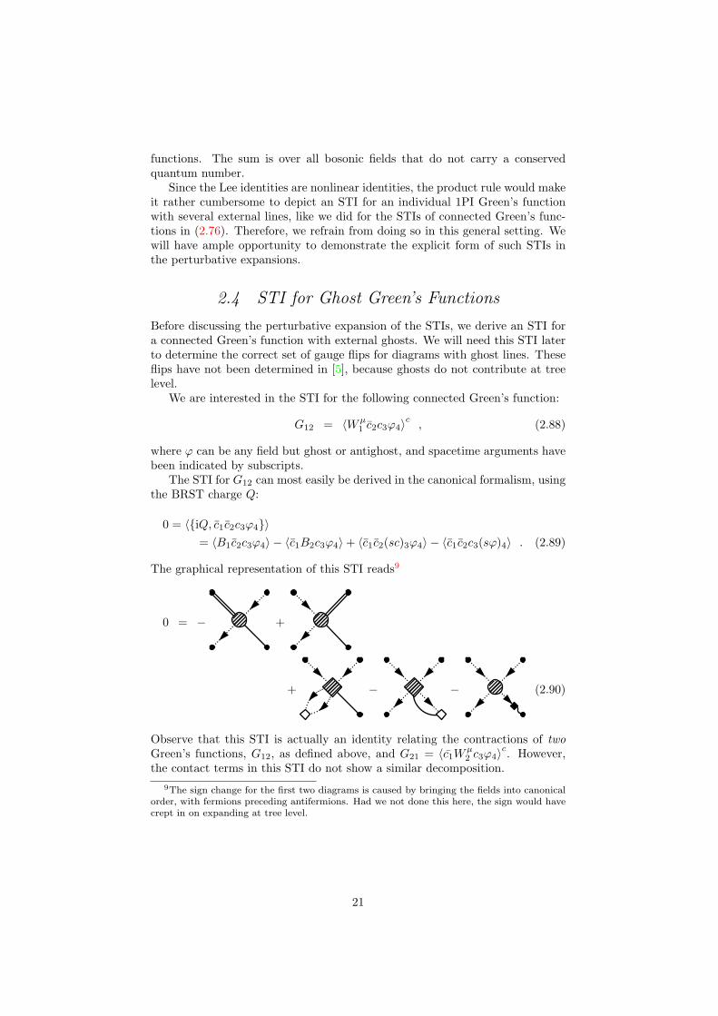
2.4 STI for Ghost Green’s Functions

Before discussing the perturbative expansion of the STIs, we derive an STI fora connected Green’s function with external ghosts. We will need this STI laterto determine the correct set of gauge flips for diagrams with ghost lines. Theseflips have not been determined in [5], because ghosts do not contribute at treelevel.

We are interested in the STI for the following connected Green’s function:

G12 = 〈Wµ1 c2c3ϕ4〉

c, (2.88)

where ϕ can be any field but ghost or antighost, and spacetime arguments havebeen indicated by subscripts.

The STI for G12 can most easily be derived in the canonical formalism, usingthe BRST charge Q:

0 = 〈iQ, c1c2c3ϕ4〉= 〈B1c2c3ϕ4〉 − 〈c1B2c3ϕ4〉+ 〈c1c2(sc)3ϕ4〉 − 〈c1c2c3(sϕ)4〉 . (2.89)

The graphical representation of this STI reads9

0 = − +

+ − − (2.90)

Observe that this STI is actually an identity relating the contractions of twoGreen’s functions, G12, as defined above, and G21 = 〈c1Wµ

2 c3ϕ4〉c. However,

the contact terms in this STI do not show a similar decomposition.9The sign change for the first two diagrams is caused by bringing the fields into canonical

order, with fermions preceding antifermions. Had we not done this here, the sign would havecrept in on expanding at tree level.

21

2.5 Perturbative Expansion

The STIs for connected Green’s functions in (2.76) and (2.90) as well as theSTIs for 1PI Green’s functions derived from the Lee identity (2.85) must beevaluated in perturbation theory.

This can be done in the standard way, for instance, by using the Gell-Man-Low formula for expressing the Green’s functions in the interaction picture,using Wick’s theorem to evaluate contractions. The resulting expansion in thecoupling constant can, as usual, be expressed through Feynman rules. In addi-tion to the normal Feynman rules of the gauge theory, however, additional rulesare necessary for the insertions of BRST transformed operators.

We have already introduced graphical notations for these operators in thelast section. Now, however, we promote these drawings from mere mnemonicdevices to representatives for analytical expressions. Consider, for instance, thehomogeneous part in the BRST transformation rule of a gauge boson W a

µ :

sW aµ

∣∣hom

= cb∆bW aµ = −gfabccbW c

µ (2.91)

The Feynman rule for this operator is just what remains when the field operatorsare taken away by contractions. Therefore, we have the rule

a, µ

b

c, ν

= −gfabcδνµ . (2.92)

In a similar way, the Feynman rules for the homogeneous parts in the BRSTtransformation laws of the other fields can be obtained. They are listed in theappendix A.

The inhomogeneous parts in the BRST transformation laws of gauge bosons,Goldstone bosons and antighosts are all expressible by means of the operatorsΘ and Θ. These operators contain derivatives. Therefore, we have to be carefulto obtain the correct momentum space Feynman rules. To this end, we definethe Fourier transforms of Θ and Θ by∫

d4x eipx Θar(x)f(x) =

(−ipµ,−Ma

)f(p) ≡ Θa

r(p)f(p) (2.93)∫d4x eipx Θa

r(x)f(x) =(

1ξa

ipµ,Ma

)f(p) ≡ Θa

r(p)f(p) . (2.94)

The sign in the exponential function of the Fourier transformation correspondsto outgoing momenta. Thus, the momentum space Feynman rules for connectedGreen’s functions are given by

p= Θr(p)

p

r(2.95)

p

r=

pΘr(p) . (2.96)

22

In both cases, the momentum p is to be interpreted as outgoing, i. e. p is directedfrom the blob to the end of the external line.

1PI Green’s functions will generally be defined with incoming momenta.This definition is actually the most useful for the following reason: The tree level1PI Green’s functions correspond precisely to the inverse propagator and theinteraction vertices of the theory. When momenta are interpreted as incoming,the interaction vertex in momentum space corresponding to particles ϕ1, ϕ2,and ϕ3 with incoming momenta p1, p2, and p3, respectively, is obtained as

Γϕ1(p1)ϕ2(p2)ϕ3(p3) . (2.97)

Had we chosen outgoing momenta, this functional derivative would correspondto an interaction vertex of three conjugate particles ϕ1, ϕ2, and ϕ3.

For 1PI Green’s functions, the correct momentum space Feynman rules forthe inhomogeneous parts in the BRST transformation laws are then, with mo-menta interpreted as incoming,

p= Θr(p)

p

r(2.98)

p

r=

pΘr(p) . (2.99)

Observe that the momentum dependence of Θ and Θ in these Feynman rulesis consistent with our earlier definitions for the action of these operators onconnected and 1PI Green’s functions. Indeed, the respective definitions differby a sign in the derivative part, which in momentum space translates into asign change of the momentum. If we replace incoming by outgoing momenta inthe Feynman rules for 1PI Green’s functions, this sign change is apparent. Theusefulness of these definitions can be appreciated in the next chapter, where wediscuss the expansion of STIs at tree level.

23

—3—Tree Level STIs and Gauge Flips

As mentioned before, the ultimate aim of our work is to show how minimalgauge invariant classes of Feynman diagrams with loops for connected Green’sfunctions in gauge theories can be constructed by employing a set of graphicalmanipulations, called gauge flips. Due to the intricacies of multi-loop diagrams,this is a complicated task. Therefore, it is essential that we decompose thistask into manageable parts, using an appropriate notation. The purpose of thepresent chapter is to introduce the corresponding decomposition and notation.To this end, we first state the STIs for the tree level vertices of the theory. Next,we demonstrate how minimal gauge invariant classes of tree Feynman diagramscan be constructed using the STIs for tree level vertices, and then provide thelink to gauge flips.

The essence of this chapter is the realization that STIs can be proven in apurely diagrammatical way, dispensing completely with any explicit analyticalexpressions. We will first demonstrate this on specific examples, then go on todevelop a systematic approach implementing this strategy for the general case.

The present chapter has some overlap with [5]. However, since our approachto the diagrammatical proof of STIs differs significantly from the one presentedin [5], we consider the inclusion of this material necessary for a self-containedpresentation of the subject.

3.1 STIs and Effective BRST Vertices

In this section we derive all STIs for the tree level vertices of the gauge theory.These identities are crucial for our later work, because we will be using tree levelidentities to show how minimal gauge invariant classes of Feynman diagrams canbe constructed in higher orders of perturbation theory, i. e. for diagrams withloops.

We begin by discussing the STIs for propagator and inverse propagator,which, of course, are closely related. Then, we derive all STIs for tree level 1PIGreen’s functions, which we shall refer to simply as vertices, because they areidentical to the interaction vertices of the gauge theory. Note that the tree levelSTIs derived in this section are collected in appendix B.

24

3.1.1 Propagator and Inverse Propagator STIs

The STIs for the full propagator and the full inverse propagator have beenderived in (2.77) and (2.87). In both cases, the homogeneous parts in the BRSTtransformation laws do not contribute at tree level. Consequently, the tree levelSTIs read, respectively

= − (3.1)

= − . (3.2)

Since we have chosen the gauge fixing term to eliminate tree level mixing be-tween gauge and Goldstone bosons, these STIs actually relate gauge boson andGoldstone boson two-point functions to the ghost two-point functions.

Of course, the STIs for propagator and inverse propagator are not indepen-dent. In fact, one could have been obtained from the other by applying theidenties

−1 = · = · . (3.3)

For good measure, we state explicitely the analytical expressions correspondingto the STIs for the inverse propagators. These are given, for gauge bosons andGoldstone bosons, respectively, by

(−ipµ)(−i)(

(p2 −M2a )gµν −

(1− 1

ξa

)pµpν

)= −

(1ξa

(−ipν))(

i(p2 − ξaM2a ))

(3.4)

(−Ma)(i(p2 − ξaM2

a ))

= − (Ma)(i(p2 − ξaM2

a )).(3.5)

3.1.2 Cubic Vertices

In the STIs for cubic vertices, there will be terms involving tree level inversepropagators multiplying tree level BRST vertices. To make the notation un-ambiguous, we cannot but introduce an extra piece of notation to make inversepropagators recognizable. We choose to do this by adding a cross at one end ofthe line representing the inverse propagator:

→ (3.6)

The STIs for physical cubic vertices, i. e. vertices without ghost lines,1 are ob-tained by taking two functional derivatives of the master identity (2.86). Theresult is

0 = + + + + .

(3.7)

1This definition of “physical” is, of course, not compatible with the notion of physical ex-ternal states. However, in the present context we find it convenient to use the term “physical”for all fields but ghosts or antighosts.

25

At this point, we emphasize that the last two terms are present only for gaugeboson and Goldstone boson lines. This feature will prove very important in thenext chapters.

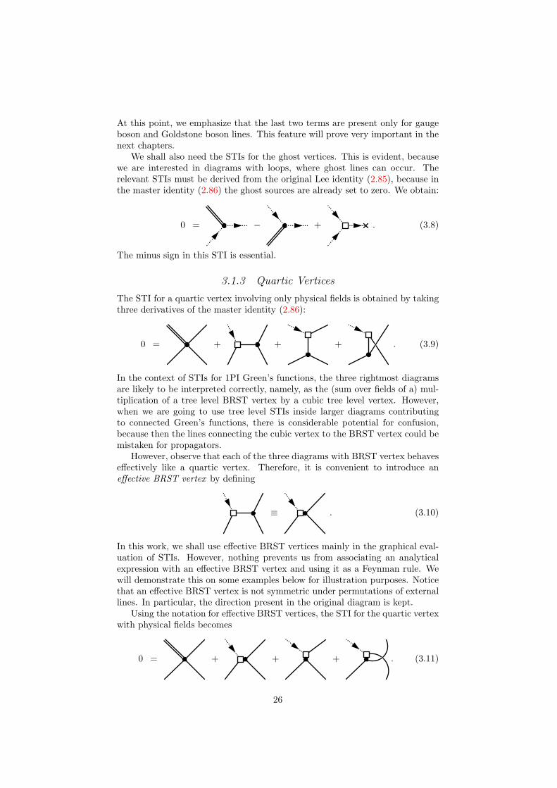
We shall also need the STIs for the ghost vertices. This is evident, becausewe are interested in diagrams with loops, where ghost lines can occur. Therelevant STIs must be derived from the original Lee identity (2.85), because inthe master identity (2.86) the ghost sources are already set to zero. We obtain:

0 = − + . (3.8)

The minus sign in this STI is essential.

3.1.3 Quartic Vertices

The STI for a quartic vertex involving only physical fields is obtained by takingthree derivatives of the master identity (2.86):

0 = + + + . (3.9)

In the context of STIs for 1PI Green’s functions, the three rightmost diagramsare likely to be interpreted correctly, namely, as the (sum over fields of a) mul-tiplication of a tree level BRST vertex by a cubic tree level vertex. However,when we are going to use tree level STIs inside larger diagrams contributingto connected Green’s functions, there is considerable potential for confusion,because then the lines connecting the cubic vertex to the BRST vertex could bemistaken for propagators.

However, observe that each of the three diagrams with BRST vertex behaveseffectively like a quartic vertex. Therefore, it is convenient to introduce aneffective BRST vertex by defining

≡ . (3.10)

In this work, we shall use effective BRST vertices mainly in the graphical eval-uation of STIs. However, nothing prevents us from associating an analyticalexpression with an effective BRST vertex and using it as a Feynman rule. Wewill demonstrate this on some examples below for illustration purposes. Noticethat an effective BRST vertex is not symmetric under permutations of externallines. In particular, the direction present in the original diagram is kept.

Using the notation for effective BRST vertices, the STI for the quartic vertexwith physical fields becomes

0 = + + + . (3.11)

26

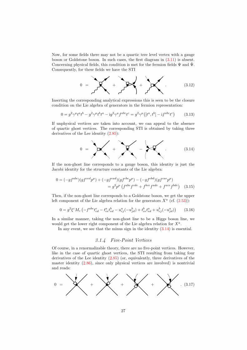
Now, for some fields there may not be a quartic tree level vertex with a gaugeboson or Goldstone boson. In such cases, the first diagram in (3.11) is absent.Concerning physical fields, this condition is met for the fermion fields Ψ and Ψ.Consequently, for these fields we have the STI

0 = + + . (3.12)

Inserting the corresponding analytical expressions this is seen to be the closurecondition on the Lie algebra of generators in the fermion representation:

0 = g2γµtatb − g2γµtbta − ig2γµfabctc = g2γµ([ta, tb]− ifabctc

)(3.13)

If unphysical vertices are taken into account, we can appeal to the absenceof quartic ghost vertices. The corresponding STI is obtained by taking threederivatives of the Lee identity (2.85):

0 = + − . (3.14)

If the non-ghost line corresponds to a gauge boson, this identity is just theJacobi identity for the structure constants of the Lie algebra:

0 = (−gfabe)(gfcedpµ) + (−gfead)(gfcbepµ)− (−gfebd)(gfcaepµ)

= g2pµ(fabefcde + f bcefade + facef bde

)(3.15)

Then, if the non-ghost line corresponds to a Goldstone boson, we get the upperleft component of the Lie algebra relation for the generators Xa (cf. (2.53)):

0 = g2ξcMc

(−fabetecd − tacet

bed − ua

cj(−ubjd) + tbcet

aed + ub

cj(−uajd))

(3.16)

In a similar manner, taking the non-ghost line to be a Higgs boson line, wewould get the lower right component of the Lie algebra relation for Xa.

In any event, we see that the minus sign in the identity (3.14) is essential.

3.1.4 Five-Point Vertices

Of course, in a renormalizable theory, there are no five-point vertices. However,like in the case of quartic ghost vertices, the STI resulting from taking fourderivatives of the Lee identity (2.85) (or, equivalently, three derivatives of themaster identity (2.86), since only physical vertices are involved) is nontrivialand reads:

0 = + + + . (3.17)

27

Here, we have again used the notion of effective BRST vertices to rewrite

≡ . (3.18)

3.2 STIs of Connected Green’s Functions: Examples

3.2.1 The STI for the Connected Three-Point Function

Denote by G3 the generic connected three-point Green’s function with at leastone external gauge boson or Goldstone boson line and only physical externallines on tree level. In terms of Feynman diagrams, G3 can be written

G3 = . (3.19)

The STI for G3 is obtained by expanding (2.76) for three external lines at treelevel:

0 = + + + +

(3.20)Actually, we could take this identity as a starting point for the analysis of STIsof Green’s functions with more external lines, instead of deriving it from STIs forthe tree level vertices. However, using this STI has the advantage of keeping thenumber of Feynman diagrams very small, making it easier to see what happens.

To begin with, we use (3.1) to replace the double line, corresponding to aninsertion of Ba, in the first diagram on the RHS. This leads to

p= −

Θr(−p)= − · . (3.21)

To understand this important relation, remember that the Feynman rules forvertices were defined for incoming momenta. On the other hand, the momentump must be interpreted as outgoing. Therefore, according to (2.98), the contrac-tion of Θr(−p) with the cubic vertex produces the first term on the RHS of theSTI (3.7).

We will encounter this pattern, which does apply at a quartic vertex in thesame way, over and over again in subsequent chapters. Therefore, it is useful tointroduce a concise and intuitive notation for the above relation. To this end,we define

· ≡ (3.22)

28

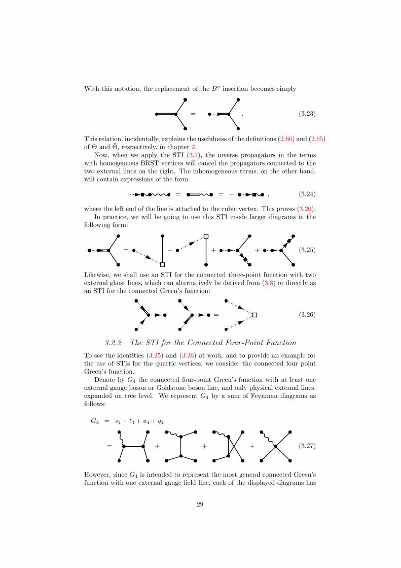
With this notation, the replacement of the Ba insertion becomes simply

= − . (3.23)

This relation, incidentally, explains the usefulness of the definitions (2.66) and (2.65)of Θ and Θ, respectively, in chapter 2.

Now, when we apply the STI (3.7), the inverse propagators in the termswith homogeneous BRST vertices will cancel the propagators connected to thetwo external lines on the right. The inhomogeneous terms, on the other hand,will contain expressions of the form

= = − , (3.24)

where the left end of the line is attached to the cubic vertex. This proves (3.20).In practice, we will be going to use this STI inside larger diagrams in the

following form:

= + + + (3.25)

Likewise, we shall use an STI for the connected three-point function with twoexternal ghost lines, which can alternatively be derived from (3.8) or directly asan STI for the connected Green’s function:

− = . (3.26)

3.2.2 The STI for the Connected Four-Point Function

To see the identities (3.25) and (3.26) at work, and to provide an example forthe use of STIs for the quartic vertices, we consider the connected four pointGreen’s function.

Denote by G4 the connected four-point Green’s function with at least oneexternal gauge boson or Goldstone boson line, and only physical external lines,expanded on tree level. We represent G4 by a sum of Feynman diagrams asfollows:

G4 = s4 + t4 + u4 + q4

= + + + (3.27)

However, since G4 is intended to represent the most general connected Green’sfunction with one external gauge field line, each of the displayed diagrams has

29

to be interpreted as a sum over all possible Feynman diagrams with the giventopology. This sum may be zero if no Feynman diagram exists according to theFeynman rules. For instance, if two external lines correspond to fermions, thediagram with quartic vertex will be absent. On the other hand, there may bemore than one Feynman diagram for a particular topology, if the propagatormay correspond to more than one field. (Remember in this context that, forour present purposes, gauge bosons and Goldstone bosons count as members ofa single field Aa

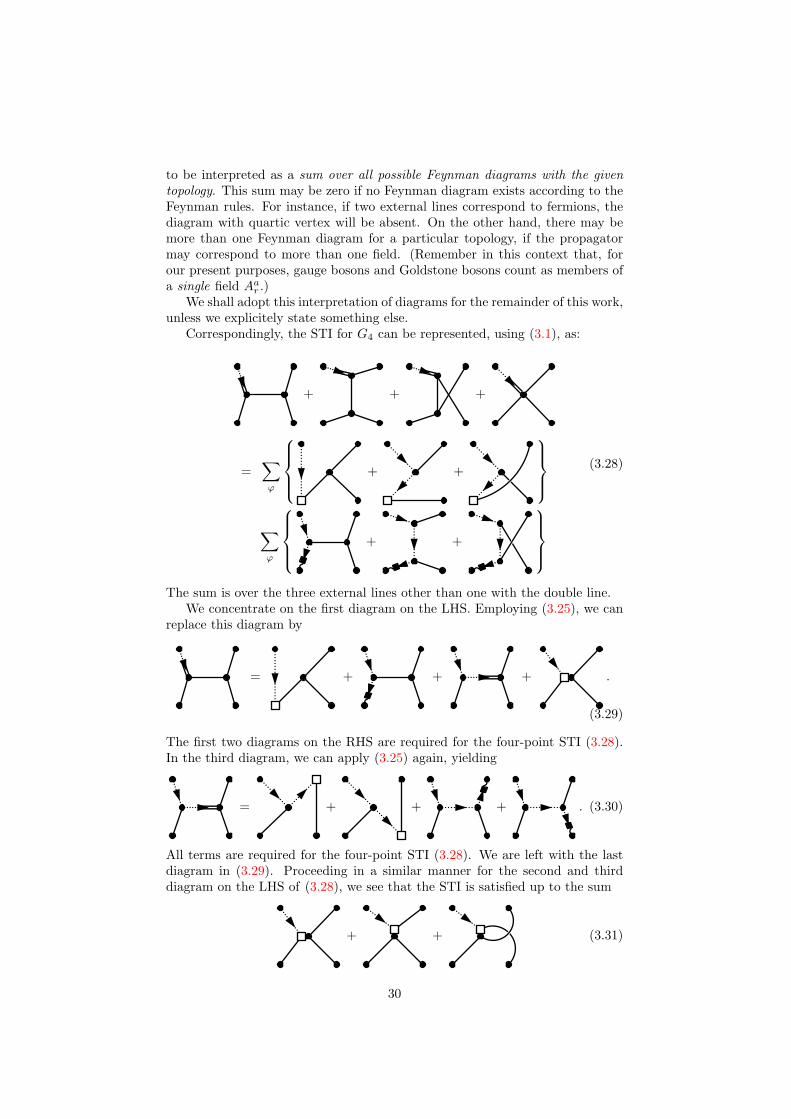
r .)We shall adopt this interpretation of diagrams for the remainder of this work,

unless we explicitely state something else.Correspondingly, the STI for G4 can be represented, using (3.1), as:

+ + +

=∑ϕ

+ +

∑ϕ

+ +

(3.28)

The sum is over the three external lines other than one with the double line.We concentrate on the first diagram on the LHS. Employing (3.25), we can

replace this diagram by

= + + + .

(3.29)

The first two diagrams on the RHS are required for the four-point STI (3.28).In the third diagram, we can apply (3.25) again, yielding

= + + + . (3.30)

All terms are required for the four-point STI (3.28). We are left with the lastdiagram in (3.29). Proceeding in a similar manner for the second and thirddiagram on the LHS of (3.28), we see that the STI is satisfied up to the sum

+ + (3.31)

30

This sum is precisely cancelled by the contribution of the diagram with quarticvertex in (3.28). To see this, just multiply the STI (3.11) by one ghost propaga-tor at the upper left line, and three propagators for the remaining, unspecifiedexternal lines.

3.3 Diagrammatical Relations

In the last section, we demonstrated on several examples how tree level STIsfor connected Green’s functions can be derived from the STIs for the vertices.Remarkably, although analytical expressions could have been inserted in eachintermediate step, we did not have to write out a single formula in order to provethe validity of the STIs. Rather, we demonstrated that a sum of diagrams couldbe obtained by making replacements in other diagrams, the ones with doublelines, according to the rules specified by vertex STIs.

In this section we will put this strategy on a sound basis. This will enableus to think and calculate entirely in terms of diagrams instead of analyticalexpressions, using an appropriate terminology. Once we have done this, we arein a good position to attack the really interesting case of Green’s functions inhigher orders of perturbation theory.

We introduce the necessary terminology in the next subsection. After that,we will define the replacement of a diagram with a double line by applyingSTIs as a map among linear combinations of diagrams. We are then going toinvestigate the properties of this map. Having established the formalism, wetreat, as our last tree level example, the connected four-point Green’s functionwith two external ghost lines. Once we have finished this, we are ready to makethe connection to gauge flips as a means of constructing gauge invariant classesof Feynman diagrams.

3.3.1 Sums and Sets

Consider an arbitrary Green’s function G. At a particular order of perturbationtheory, G has an expansion in terms of Feynman diagrams with a fixed number ofloops. We denote by F (G) the set of all diagrams contributing to this expansion,leaving the number of loops implicit. F (G) is called the forest of G.

Given the forest F (G) of Feynman diagrams, we define the Green’s functionG itself as

G =∑

d∈F(G)

χ(d)d . (3.32)

In this expression, the weight factor χ(d) is the product of symmetry factorsand fermion loop signs pertaining to the diagram d according to the Feymmanrules. Note, that we really define G as a linear combination of diagrams, notof the corresponding analytical expressions. (Although the transition from theformer to the latter is, of course, trivial.)

Now consider a Green’s function G with an external gauge boson line. Ingeneral, we can extract from G a contribution to a scattering amplitude of aphysically polarized gauge boson. Replace the gauge boson by the unphysi-cal linear combination Ba (the gauge fixing functional), and call the resultingGreen’s function Θ(G).2 There is a corresponding STI, in which Θ(G) is set

2The use of the symbol Θ will be justified in the next subsection.

31

equal to a sum over Green’s functions with insertion of a single BRST trans-formed operator. We denote this sum by W(G) and refer to it as the contactterms of the STI. For instance, in the STI for the propagator 〈W a

µWbν 〉

c,

0 = 〈BaW bν 〉

c+ 〈ca(sW b

ν )〉c , (3.33)

we haveΘ(G) = 〈BaW b

ν 〉c

and W(G) = 〈ca(sW bν )〉c . (3.34)

We define the expansions of Θ(G) andW(G) in complete analogy to the expan-sion (3.32) of G:

Θ(G) =∑

d∈F(Θ(G))

χ(d)d (3.35)

W(G) =∑

d∈F(W(G))

χ(d)d (3.36)

The point of these definitions is that they allows us to formally consider con-tributions to Green’s functions or STIs as elements in the free vector spaceof Feynman diagrams, with rational coefficients. This construction is well de-fined, because the Feynman rules instruct us to sum over topologically differentFeynman diagrams only, such that the underlying Feynman diagrams are re-ally linearly independent. The statement that a certain linear combination ofFeynman diagrams vanishes has a precise and unambigous meaning in this con-text: The coefficient of every diagram in the linear combination must vanishseparately.

On the other hand, for some purposes it is convenient to be able to use setterminology for the Green’s functions G, Θ(G) orW(G). A particular example,which we shall encounter in this work, concerns the question whether a givendiagram can be produced by replacing the contracted external line in anotherdiagram according to the vertex STIs, irrespective of the coefficients. We willsoon define this replacement as a map in the free vector space of Feynmandiagrams. The question could then be formulated in the language of linearcombinations as follows: d is contained in a sum S of diagrams if it appears inS with a nonvanishing coefficient. Such phrases could only avoided by definingthe abovementioned map for sets of Feynman diagrams, too.

Therefore, we shall use set terminology in connection with G, Θ(G) andW(G) in an intuitive sense. In particular, we will say that a diagram d iscontained in a Green’s function G. Also, we will say that a set of Feynmandiagrams satisfies an STI, implying that the STI is satisfied by the sum over alldiagrams with corresponding coefficients.

Note, however, that relations among linear combinations of diagrams willnever be understood in the set theoretical sense. Thus, if we write down anequality between two expansions in Feynman diagrams, we always mean equalityof coefficients for every Feynman diagram in the sum.

As a simple example, consider the gauge boson self energy Πµν in a pureYang-Mills theory. In dimensional regularization, there are just two nonzerodiagrams. Thus,

F (Πµν) =

,

(3.37)

32

The Green’s function itself is expanded as

Πµν =12

− . (3.38)

Πµν satisfies the STI (2.86), evaluated at one-loop level. The statement thatthe set (3.37) satisfies the STI will be taken to mean just that.

3.3.2 Contraction as Map

In the previous section, we have defined the Green’s function Θ(G) as theGreen’s function obtained from G by replacing a certain gauge boson by theunphysical linear combination Ba of gauge bosons and Goldstone bosons. Werefer to this replacement as contraction, since it amounts to contracting theoperator Θr or Θr with a Green’s function of the (formally) five dimensionalgauge field Ar.

The STI for the Green’s function G expresses the statement that the sumof the contraction Θ(G) and the contact terms W(G) is a vanishing linear com-bination of Feynman diagrams. We have already seen in the explicit tree levelexamples of section 3.2, that the contraction produces a sum of diagrams fromeach diagram contributing to G. It is therefore natural to consider the contrac-tion as a linear map Θ in the space of linear combinations of Feynman diagrams.We use the same symbol here as for the operators Θr and Θr to emphasize theclose relationship.3 The use of different symbols for connected and 1PI Green’sfunctions is unnecessary here, because it will always be clear from the contextwhich one applies.

We now have to give a definition of the map Θ. Since Θ is assumed to belinear, it suffices to define it for a single diagram d contributing to G. Recallhow, in the derivation of the STI for the four-point function, we had to usethe STI (3.7) repeatedly (cf. the discussion around (3.29) and (3.30)). Thisis the general pattern: The sum of diagrams Θ(d) will always be obtained byrepeatedly applying contractions at vertices of d.

To formalize this observation, we define the elementary contraction θ of avertex to extract the homogeneous parts in the tree level STIs:

θ ≡ + (3.39)

θ

≡ (3.40)

In particular, for the quartic vertex θ is equal to the full contraction. On theother hand, for the cubic vertex we have

0 = +θ

+ + . (3.41)

3In fact, for the analytical expressions corresponding to G, the operators Θr and Θr dothe same as the operator Θ for the formal linear combination of Feynman diagrams.

33

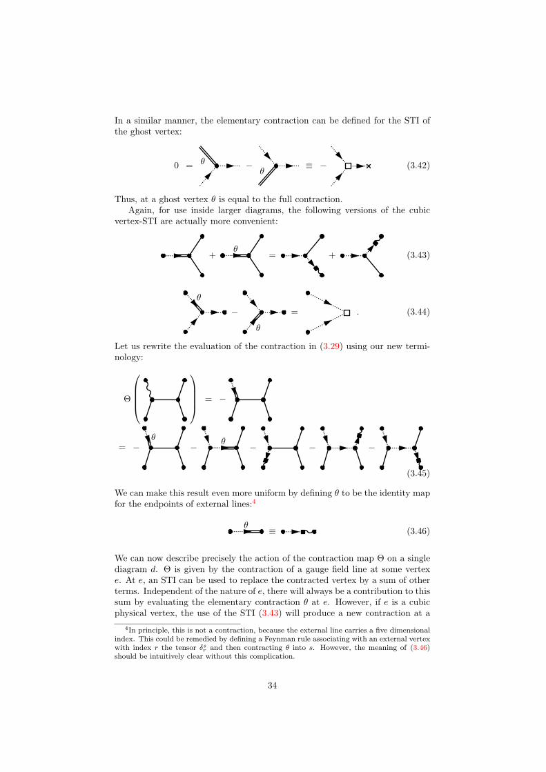
In a similar manner, the elementary contraction can be defined for the STI ofthe ghost vertex:

0 = θ −θ

≡ − (3.42)

Thus, at a ghost vertex θ is equal to the full contraction.Again, for use inside larger diagrams, the following versions of the cubic

vertex-STI are actually more convenient:

+θ

= + (3.43)

θ

−

θ

= . (3.44)

Let us rewrite the evaluation of the contraction in (3.29) using our new termi-nology:

Θ

= −

= −θ

− θ − − −

(3.45)

We can make this result even more uniform by defining θ to be the identity mapfor the endpoints of external lines:4

θ ≡ (3.46)

We can now describe precisely the action of the contraction map Θ on a singlediagram d. Θ is given by the contraction of a gauge field line at some vertexe. At e, an STI can be used to replace the contracted vertex by a sum of otherterms. Independent of the nature of e, there will always be a contribution to thissum by evaluating the elementary contraction θ at e. However, if e is a cubicphysical vertex, the use of the STI (3.43) will produce a new contraction at a

4In principle, this is not a contraction, because the external line carries a five dimensionalindex. This could be remedied by defining a Feynman rule associating with an external vertexwith index r the tensor δs

r and then contracting θ into s. However, the meaning of (3.46)should be intuitively clear without this complication.

34

neighboring vertex v, if e is connected to v by a gauge boson or Goldstone bosonline. At v, we can evaluate the contraction in exactly the same way. Observethat, in this process, the gauge boson or Goldstone boson line connecting e andv is replaced by a ghost line. This process is recursively iterated. The recursionterminates, when no more cubic vertex with outgoing gauge field lines can bereached from another contracted vertex.

When the recursion stops, Θ(d) will be expressed as a sum of diagrams, eachof which can be characterized uniquely in the following way. Define a path ind as a sequence of gauge field propagators, connecting e to some vertex v of dvia cubic vertices, such that no propagator appears twice. In particular, thisimplies that a path always starts at an external vertex. Evidently, the recursiveevaluation of Θ(d) will eventually proceed along every path in d. Also, if a vertexw cannot be reached by a path, there will be no term in Θ(d) corresponding toa contraction at w. As an example, consider the following diagram, where allgauge bosons have been made explicit:

d =

e

24

53

1 (3.47)

There are three paths in this diagram, which we indicate in by drawing thecorresponding gauge field propagators in a bold line style:

e

24

53

1

e

24

53

1

e

24

53

1

P1 = e, 1 P2 = e, 1, 2 P3 = e, 1, 3

(3.48)

The vertices 4 and 5, on the other hand, cannot be reached by any path. Thus,the contraction Θ(d) will decompose into a sum over contributions of the pathsP1, P2, and P3.

Consider now the evaluation of the elementary contraction θ at the endpointv of a path P . If v is an external vertex, θ will produce a single term accordingto (3.46). If v is a cubic vertex, θ produces a sum of two diagrams:

θn1

n2

n3

v = −n1

n2

n3

−n1

n2

n3

(3.49)

Either of the two diagrams on the RHS can be identified uniquely by specifyingthe second propagator, apart from the ghost propagator, coincident with theeffective BRST vertex. These are (n3, n2) for the first diagram as well as (n2, n3)

35

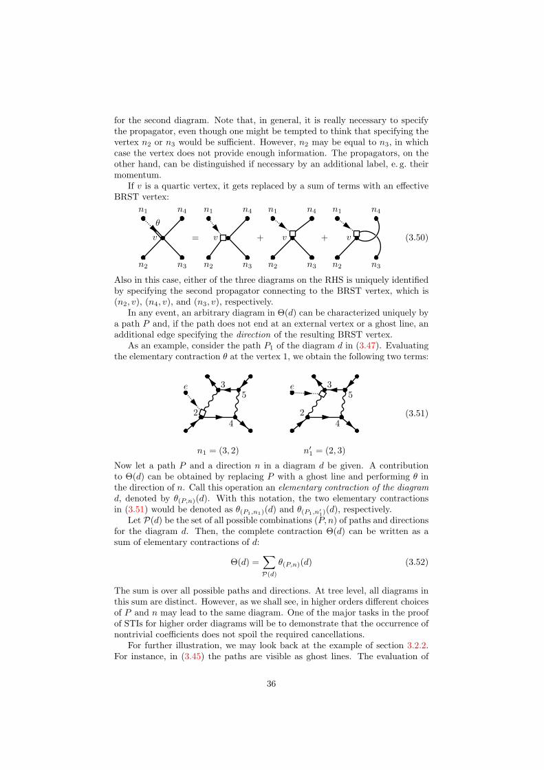
for the second diagram. Note that, in general, it is really necessary to specifythe propagator, even though one might be tempted to think that specifying thevertex n2 or n3 would be sufficient. However, n2 may be equal to n3, in whichcase the vertex does not provide enough information. The propagators, on theother hand, can be distinguished if necessary by an additional label, e. g. theirmomentum.

If v is a quartic vertex, it gets replaced by a sum of terms with an effectiveBRST vertex:

θ

n1 n4

n2 n3

v =

n2

n1

n3

n4

v +

n2

n1

n3

n4

v +

n2

n1

n3

n4

v (3.50)

Also in this case, either of the three diagrams on the RHS is uniquely identifiedby specifying the second propagator connecting to the BRST vertex, which is(n2, v), (n4, v), and (n3, v), respectively.

In any event, an arbitrary diagram in Θ(d) can be characterized uniquely bya path P and, if the path does not end at an external vertex or a ghost line, anadditional edge specifying the direction of the resulting BRST vertex.

As an example, consider the path P1 of the diagram d in (3.47). Evaluatingthe elementary contraction θ at the vertex 1, we obtain the following two terms:

e

24

53 e

24

53

n1 = (3, 2) n′1 = (2, 3)

(3.51)

Now let a path P and a direction n in a diagram d be given. A contributionto Θ(d) can be obtained by replacing P with a ghost line and performing θ inthe direction of n. Call this operation an elementary contraction of the diagramd, denoted by θ(P,n)(d). With this notation, the two elementary contractionsin (3.51) would be denoted as θ(P1,n1)(d) and θ(P1,n′

1)(d), respectively.

Let P(d) be the set of all possible combinations (P, n) of paths and directionsfor the diagram d. Then, the complete contraction Θ(d) can be written as asum of elementary contractions of d:

Θ(d) =∑P(d)

θ(P,n)(d) (3.52)

The sum is over all possible paths and directions. At tree level, all diagrams inthis sum are distinct. However, as we shall see, in higher orders different choicesof P and n may lead to the same diagram. One of the major tasks in the proofof STIs for higher order diagrams will be to demonstrate that the occurrence ofnontrivial coefficients does not spoil the required cancellations.

For further illustration, we may look back at the example of section 3.2.2.For instance, in (3.45) the paths are visible as ghost lines. The evaluation of

36

the elementary contraction θ in the first and second diagram can be read fromrelations (3.29) and (3.30). As an example of an elementary contraction at aquartic vertex, cf. (3.31).

Equation (3.52) defines the action of Θ on a single diagram. Its action on alinear combination of diagrams is then defined in an obvious way by linearity.

Evidently, we do not learn anything new about the STI of G4 in this termi-nology. The point of the decomposition of Θ(d) in terms of elementary contrac-tions is that it allows for a reorganization which will simplify the diagrammaticalproof of STIs immensely.

3.3.3 Decomposing the Contraction Map Θ

In this section, we show how the contraction Θ as well as the elementary con-traction θ, of diagrams as well as vertices, can be decomposed in such a waythat the production of contact terms can be disentangled from the cancellationsoccurring in the diagrammatical proofs of STIs.

In section 3.2.2 we showed how the diagrams in the four point Green’s func-tion G4 conspire to produce the contact terms W(G4) of the STI when the con-traction Θ(G4) is evaluated. In general, Θ(d) for a single diagram d containedcontact term diagrams as well as diagrams that had to cancel in order for theSTI to be satisfied. The cancellation was then achieved by picking appropriateterms from the contributions of all diagrams.

While this approach ultimately worked, the proof of the STIs can be arrangedmuch clearer by separating the production of contact term diagrams from thecancellations. The basic idea is the following: Let G be some connected Green’sfunction and W(G) the sum of contact terms. The contraction Θ(G) is givenby

Θ(G) =∑d∈G

χ(d)Θ(d) =∑d∈G

χ(d)∑P(d)

θ(P,n)(d) , (3.53)

with χ(d) the weight factor of the diagram d.We now decompose Θ(G) as follows:

Θ(G) = Ω(G) + B4(G) + B5(G) + Bc(G) (3.54)

We define the various maps in this sum for single diagrams and then extend bylinearity. Then, let G be some Green’s function and d a diagram in d. If G hasno external ghost lines, Ω(d) is the sum over all diagrams in Θ(d) with one ofthe following subdiagrams at the end of external lines:

θ(3.55a)

(3.55b)

For Green’s functions with external ghost lines, we include, in addition, diagramswith an elementary contraction at a ghost line, if the outgoing ghost line is an

37

external line (indicated here by an open circle):

θ

n

(3.55c)

B4(d) is the sum over all diagrams in Θ(d) with a quartic effective BRST vertexwithout extra ghost lines:

, (3.56)

B5(d) is the sum over all diagrams in Θ(d) with a five-point effective BRSTvertex:

. (3.57)

Finally, Bc(d) is the sum over all diagrams in Θ(d) with either an elementarycontraction at a ghost line or an effective BRST vertex with extra ghost lines,but not if the outgoing ghost line is an external line:

θ

n

(3.58a)

(3.58b)

Given the decomposition (3.54) of Θ(G), the STI Θ(G) +W(G) = 0 can beverified by proving separately Ω(G)+W(G) = 0 and B4(G)+B5(G)+Bc(G) = 0.We will do this in the next chapter.

First, however, we show how the various terms in the decomposition canbe expressed quite naturally as sums over decomposed elementary contractions.To this end, consider again a single diagram d. Clearly, it is possible to expressΩ(d) as a sum over paths and directions. Now, however, only those combinations(P, n) are selected, for which the contraction θ(P,n) satisfies the correspondingcriteria. Denote the set of such combinations (P, n) by PΩ(d). Then

Ω(d) =∑PΩ(d)

θ(P,n)(d) . (3.59)

It is possible to eliminate the restriction on the summed paths by defining anelementary contraction ω as follows:

ω(P,n)(d) =θ(P,n)(d) for (P, n) ∈ PΩ(d)

0 for (P, n) /∈ PΩ(d) (3.60)

38

In complete analogy, we define the restricted path sets PB4(d), PB5(d), andPBc

(d), as well as the elementary contractions β4, β5 and βc. Obviously, P isthe disjoint union of the restricted path sets:

P(d) = PΩ(d) ∪ PB4(d) ∪ PB5(d) ∪ PBc(d) (3.61)

Therefore, we have the following decomposition of the elementary contractionsθ of d:

θ(P,n)(d) = ω(P,n)(d) + (β4)(P,n)(d) + (β5)(P,n)(d) + (βc)(P,n)(d) . (3.62)

For every pair (P, n), exactly one of the terms in this sum is nonzero.Finally, the decomposition (3.62) of elementary contractions θ(P,n)(d) of di-

agrams induces a corresponding decomposition of the elementary contraction θof a single vertex. For instance, β4 will perform only replacements that lead toa subdiagram of the form (3.56).

For many purposes, it is useful to decompose the elementary contraction β4

further into β43 and β44 according to the origin of the quartic BRST vertex. Inparticular, β43 will act only at a cubic vertex:

β34

= + . . . (3.63)

β44, on the other hand, will produce quartic BRST vertices from quartic vertices:

β44

= − − − (3.64)

Accordingly, we decompose the elementary contraction (β4)(P,v) into (β43)(P,v)

and (β44)(P,v). Likewise, B4 is split into B43 and B44.The foregoing discussion might appear very formal. However, there is a very

intuitive explanation for what our definitions achieve. Suppose we are interestedin how the diagrams in B4(G), i. e. with subdiagrams of the form (3.56), canbe produced by applying STIs in the diagrams of G. Of course, we could justrecursively evaluate the contraction Θ(d) as described in the last subsection,throwing away all undesired diagrams. A better approach would be to just pro-duce the desired contractions, ignoring paths (P, n) which would not contributeto B4(G). The neglected elementary contractions can then be picked up laterby one of the remaining maps. The above definitions just formalize this simpleidea.

3.4 The STI for the Two-Ghost Four-Point Function

In this section, we use the formalism developed in the last section to verify theSTI (2.90) for the connected four-point Green’s function G12 with two externalghost lines at tree level. This will enable us to derive gauge flips for diagramsexternal ghost lines.

39

First, we write down the expansion of G12 at tree level:

G12 = s12 + t12 + u12 = + + (3.65)

The names have been introduced for future reference. G21 is obtained from G12

by exchanging the gauge field line with the incoming ghost line:

G21 = s21 + t21 + u21 = + + (3.66)

The contact terms of the STI (2.90), evaluated at tree level, are given by

W(G12) = − W(G21) = − +

− − + + . (3.67)

To verify the STI (2.90) at tree level, we have to show that

Θ(G12)−Θ(G21) =W(G12) . (3.68)

To begin with, let us note that B4 and B5 are identically zero in this case, theformer because every elementary contraction of a diagram will involve a ghostline, the latter because there are no five-point subdiagrams.

Next consider Bc. For s12, we have

Bc(s12) = Θ(s12) = −

βc

. (3.69)

Doing the same for s21 and using the STI (3.26), we get

Bc(s12)− Bc(s21) = − . (3.70)

Then, we have

Bc(u12) = − (3.71)

40

Bc(t21) = − (3.72)

On the remaining diagrams, Bc gives zero. Collecting the contributions to Bc,we get a cancellation by making use of the STI (3.14):

Bc(s12)− Bc(s21) + Bc(u12)− Bc(t21) = 0 (3.73)

Finally, we have to evaluate the contributions of Ω. From t21, we get

Ω(t21) = − − − ω. (3.74)

Next evaluate the contribution from t12:

Ω(t12) = −ω

(3.75)

Using (3.26), we can add up the two contributions to get

Ω(t12)− Ω(t21) = + − . (3.76)

This is precisely one half of the contact terms. Doing the same manipulationsfor u12 and u21 we arrive at

Ω(t12) + Ω(u12)− Ω(t21)− Ω(u21) =W(G12) . (3.77)

We have exhausted all nonzero contributions to Θ(G12) and Θ(G21). Therefore,the STI (3.68) is proven.

3.5 Gauge Cancellations and Gauge Flips

In this section, we want to make a connection between cancellations in the STIsfor G4 on the one hand and G12 as well as G21 on the other hand, and gaugeflips. We have already established a notation for the diagrams in these Green’sfunctions (cf. (3.27), (3.65), and (3.66)).

Let us briefly recall the derivation of the STI for G4, using the terminologydeveloped above: The contact terms W(G4) are produced by Ω, i. e. we haveΩ(G4) +W(G4) = 0. B5(G4) and Bc(G4) are identically zero, the former dueto lack of a sufficient number of external lines, the latter due to the absence ofghost lines. B4 is split into B43 and B44 according to (3.63) and (3.64). Now

41

B43 yields zero on q4, while B44 yields zero on s4, t4 and u4. The remainingnonzero contributions cancel precisely:

B43(s4) + B43(t4) + B43(u4) + B44(q4) = 0 (3.78)

This relation clearly shows that no real subset S of G4 can satisfy the STI onits own.5 For this to be true, S would have to satisfy

Θ(S) = Ω(S) . (3.79)

But this impliesB4(S) = 0 , (3.80)

which is impossible for a real subset of G4 according to (3.78).We can put it another way. If we start with one diagram, s4 say, and

require that diagrams be added until (3.79) holds, we see that we are successivelyforced to add t4, u4, and q4 as well. Now elementary gauge flips are definedas the possible transformations among elements of F (G4). Therefore, we canexpress this result as the statement that all possible elementary gauge flipsmust be applied to s4 in order to obtain a set of diagrams satisfying (3.79).This demonstrates the connection between gauge cancellations and elementarygauge flips for G4.

Next we are going to derive elementary gauge flips for diagrams in G12 byconsidering the cancellations in the STI (3.68) for G12 and G21. Since this isan STI for two Green’s functions at the same time, we need to find a general-ization of the requirement (3.79) for a subset of diagrams to satisfy the STI byitself. Denoting by S12 and S21 subsets of G12 and G21, respectively, a naturalgeneralization would be to demand

Θ(S12)−Θ(S21) = Ω(S12)− Ω(S21) . (3.81)

However, this requirement is actually not sufficient to guarantee that the RHSis a subset of the contact termsW(G12). To see this, observe that, for diagramswith ghost lines, ω does not produce a contact term directly when applied toa single diagram in G12. Rather, we must subtract the contribution of a corre-sponding diagram in G21 to get a contact term. We have seen this explicitelyin (3.76). Therefore, (3.81) has to be supplemented by the constraint that theRHS must be contained in the contact terms W(G12).

A glance at (3.73) shows that the cancellations alone already select twodiagrams each from G12 and G21. The supplementary constraint then forces usto choose all of G12 and G21. Since elementary gauge flips for diagrams withtwo external ghost lines are precisely the transformations among diagrams inG12 (or, equivalently, G21), this is again equivalent to the statement that (3.81)can only be satisfied by a set which is invariant under elementary gauge flips.

Before closing this section, let us comment on two points. First, the readerfamiliar with the literatur on gauge flips may wonder why we did not discuss el-ementary gauge flips among four-point diagrams with four external ghost lines.The reason is that, as we shall see in the next chapters, these are really notneeded to prove the STIs we consider. However, for more general STIs (e. g.

5Here and in the rest of this section, we make extensive use of set terminology for Green’sfunctions. For a justification, cf. section 3.3.1.

42

STIs with several contractions), or in the study of the gauge parameter depen-dence of Green’s functions, the situation may be different. As a second remark,we note that the STI for the (non-existent) five-point vertices has not been usedup to this point, because we only considered four-point Green’s function on treelevel. However, this STI plays a crucial role in the gauge cancellations alreadyat tree level [5]. Likewise, it will have to do its part in the case of higher orderdiagrams.

3.6 Projections

Before we enter into the discussion of gauge cancellations in higher order dia-grams, we introduce yet one more useful tool. Clearly, it would be desirableif we did not have to consider all diagrams of a Green’s function at once. Tothis end, observe that an elementary contraction θ of a diagram d preservesmany properties of d. In particular, although θ exchanges cubic gluon verticesby ghost gluon vertices (and propagators accordingly) on the path to the con-tracted vertex, this does not change the total number of cubic vertices. When θacts on a vertex inside d, it may remove a propagator, joining two cubic verticesinto an effective BRS vertex. Essentially, this produces a quartic vertex fromtwo cubic ones. But this can happen only once for every elementary contractionof d. Consequently, cancellations can only take place among diagrams for whichthe number of quartic vertices differs by one. We have seen an example of thisin the discussion of the STI for G4 in section 3.2.2.

Therefore, it makes sense to consider for a Green’s function G the subset ofdiagrams with exactly ν quartic vertices. More precisely, since G is an elementof the free vector space over Feynman diagrams, we can consider the projectionof G onto the subspace of diagrams with ν quartic vertices. We will denote thisprojection as

[G]ν . (3.82)

There is another important property of a diagram d that can only be changedin a very controlled way, namely, the number ρ of ghost loops. Of course, thisis irrelevant on tree level. However, decomposing a connected Green’s functionaccording to the number of ghost loops will simplify the proof of cancellationsinvolving the STIs for ghost vertices a lot. Therefore, we introduce a projectionof G on the subspace of diagrams with ρ ghost loops, denoted as

[G]ρ . (3.83)

Clearly, both projections are independent. Therefore we can consider the sub-space of diagrams with ν quartic vertices and ρ ghost loops. The projection ofG onto that subspace is then

[G]νρ . (3.84)

The contact terms W(G) can be projected in the same way.If the theory contains physical fermions, the number of fermion loops is

actually preserved by elementary contractions. In principle, then, we could in-troduce a further projection onto the subspace of diagrams with a fixed numberof fermion loops. However, because this number does not change at all, all rela-tions among diagrams will hold separately in each subspace. We can thereforeleave this decomposition implicit.

43

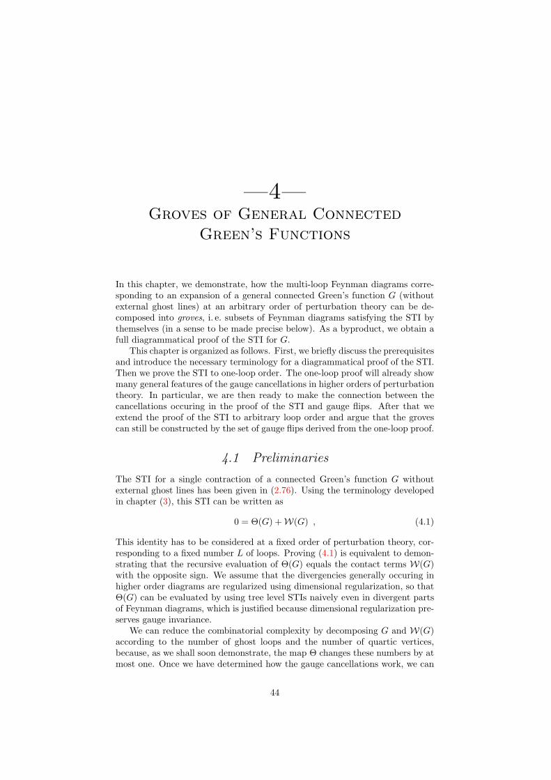
—4—Groves of General Connected

Green’s Functions

In this chapter, we demonstrate, how the multi-loop Feynman diagrams corre-sponding to an expansion of a general connected Green’s function G (withoutexternal ghost lines) at an arbitrary order of perturbation theory can be de-composed into groves, i. e. subsets of Feynman diagrams satisfying the STI bythemselves (in a sense to be made precise below). As a byproduct, we obtain afull diagrammatical proof of the STI for G.

This chapter is organized as follows. First, we briefly discuss the prerequisitesand introduce the necessary terminology for a diagrammatical proof of the STI.Then we prove the STI to one-loop order. The one-loop proof will already showmany general features of the gauge cancellations in higher orders of perturbationtheory. In particular, we are then ready to make the connection between thecancellations occuring in the proof of the STI and gauge flips. After that weextend the proof of the STI to arbitrary loop order and argue that the grovescan still be constructed by the set of gauge flips derived from the one-loop proof.

4.1 Preliminaries

The STI for a single contraction of a connected Green’s function G withoutexternal ghost lines has been given in (2.76). Using the terminology developedin chapter (3), this STI can be written as

0 = Θ(G) +W(G) , (4.1)

This identity has to be considered at a fixed order of perturbation theory, cor-responding to a fixed number L of loops. Proving (4.1) is equivalent to demon-strating that the recursive evaluation of Θ(G) equals the contact terms W(G)with the opposite sign. We assume that the divergencies generally occuring inhigher order diagrams are regularized using dimensional regularization, so thatΘ(G) can be evaluated by using tree level STIs naively even in divergent partsof Feynman diagrams, which is justified because dimensional regularization pre-serves gauge invariance.

We can reduce the combinatorial complexity by decomposing G and W(G)according to the number of ghost loops and the number of quartic vertices,because, as we shall soon demonstrate, the map Θ changes these numbers by atmost one. Once we have determined how the gauge cancellations work, we can

44

use this information to define the correct set of gauge flips for the constructionof minimal gauge invariant subsets of F (G).

4.2 STI at One-Loop

In this section we take G and W(G) to refer to their respective expansions inone-loop Feynman diagrams. Using the decomposition (3.54), we will verify theSTI (4.1) by successively proving the following statements:

Ω(G) +W(G) = 0 (4.2a)B4(G) = 0 (4.2b)B5(G) = 0 (4.2c)Bc(G) = 0 (4.2d)

4.2.1 Production of Contact Terms

We begin by proving (4.2a), which states that the production of contact termsis entirely described by the action of Ω. From the defining contractions (3.55) ofΩ it is obvious that these contractions can change neither the number of quarticvertices nor the number of ghost loops. For the elementary contraction ω is zeroat a quartic vertex or ghost vertex. Therefore, (4.2a) must hold separately forevery projection [G]νρ of G. Since we can project the contact termsW(G) in thesame way, we have to show

Ω([G]νρ

)+ [W(G)]νρ = 0 . (4.3)

For notational convenience, however, we shall continue to write G instead of[G]νρ, and likewise forW(G), in the remainder of this section, the decompositionbeing implicitely understood. We can do so safely, because Ω preserves ν andρ.

We are going to verify (4.3) in two steps. First, we demonstrate that for everydiagram d in G, Ω(d) is contained in W(G) with the opposite sign. (Formally,this means that the projection of Ω(d) +W(G) onto Ω(d) vanishes.) In thesecond step, we show that every diagram inW(G) can be produced by applyingan elementary contraction ω to some d in G. These two statements clearly implythe relation (4.3).

Every diagram produced by applying an elementary contraction ω(P,v) to din G constitutes a valid Feynman diagram for W(G). This is clear, because theforest F (W(G)) consists of all diagrams with a subdiagram (3.55a) or (3.55b)in place of an external line, with the ghost line replacing a gauge field lineoriginating at the contracted external gauge field line. Note that this argumentis actually independent of the number L of loops. Furthermore, the relative signbetween ω(P,v)(d) and the corresponding contribution toW(G) is caused by therelation (3.23). Consequently, we need only show that every nonzero ω(P,v)(d)is produced with the correct symmetry factor. (Since the number ρ of ghostloops is preserved by ω, the sign of the weight factor is automatically correct.)

Let d′ = ω(P,v)(d). d′ will have the same symmetry factor as d unless theghost line in d′ destroys an automorphism of d. This can happen because aghost line is always directed while the gauge field line it replaces may be not, if

45

the gauge field is neutral. Examples are provided by the gluon ghosts in QCDor the ghosts of photon and Z0 in the SM.

At one loop level, d can only have a nontrivial automorphism if it containsone of the following tadpole or self energy diagrams as subdiagram:

(4.4)

Among these, only in the rightmost diagram, i. e. the self energy, can the pathP pass through the loop. For definiteness, we consider the case of the gluonself energy in QCD. Now, while the gluon self energy has a symmetry factor1/2, the ghost self energy has not. On the other hand, there are two equivalentpaths through the gluon self energy. Both paths are appear in the sum Ω(d),whence the ghost self energy is produced twice:

Ω−→ + (4.5)

Thus, the symmetry factor is cancelled, and consequently d′ will be producedwith the correct symmetry factor of unity. This shows that Ω(G) is containedin W(G).

We are not yet ready, however, because in principle it would be possiblethat there exists a diagram d′ in W(G), which is not in Ω(G). This is, however,impossible, because given d′ in W(G) we can always reverse the contraction byreplacing the ghost line by a gauge field line and reading the definition of theelementary contraction ω backwards. This process will give us a valid Feynmandiagram for G. (Although not necessarily with the correct weight, but that doesnot matter here.) Consequently, d′ must be in Ω(G). This completes the proofof (4.3), hence (4.2a).

In the next sections, we will verify the remaining relations of (4.2). The proofof these relation is actually at the heart of this work, because it will disclose thegauge cancellations among various diagrams, thus allowing us to justify the useof gauge flips in constructing gauge invariant classes of Feynman for one loopprocesses.

4.2.2 Cancellations in B4(G)

In this section, we are going to verify the validity of (4.2b). We have seen anexplicit example of the cancellations in B4(G4) in the derivation of the STI forthe four-point Green’s function G4 on tree level in chapter 3. This identity is arelation for offshell values of the external momenta. Therefore, the same cancel-lation would take place among four larger diagrams related to each other by theexchange of a single four-point subdiagram, chosen from the set s4, t4, u4, q4of diagrams constituting F (G4). Indeed, this observation is the basis for theconstruction of gauge invariant classes of Feynman diagrams in the tree levelcase.[4][5]

It is reasonable to expect that in the one loop case, too, similar cancellationstake place among diagrams for which the number of quartic vertices differs byone, irrespective of the number of ghost loops. Indeed, we shall now prove that

B43

([G]ν

)+ B44

([G]ν+1

)= 0 . (4.6)

46

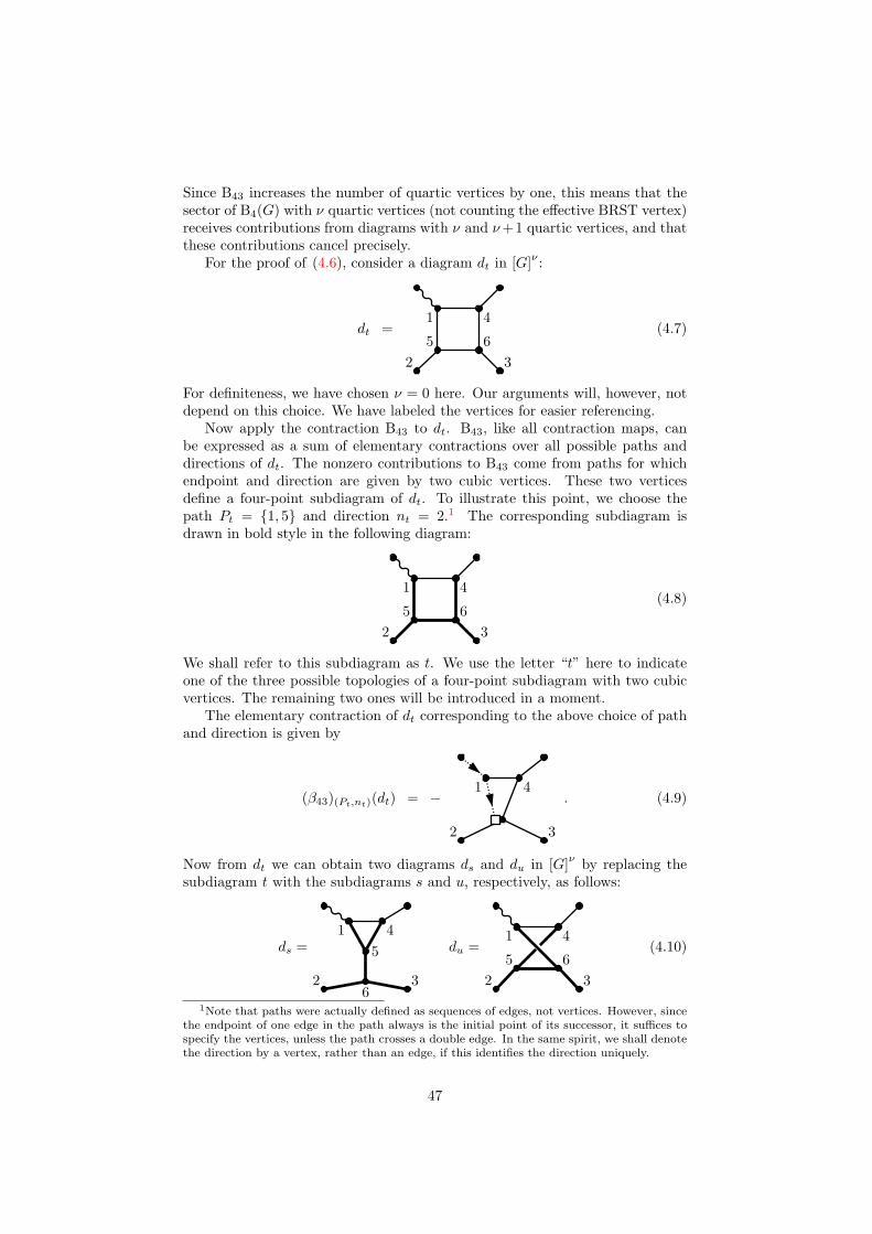
Since B43 increases the number of quartic vertices by one, this means that thesector of B4(G) with ν quartic vertices (not counting the effective BRST vertex)receives contributions from diagrams with ν and ν+1 quartic vertices, and thatthese contributions cancel precisely.

For the proof of (4.6), consider a diagram dt in [G]ν :

dt =

2 35 6

1 4(4.7)

For definiteness, we have chosen ν = 0 here. Our arguments will, however, notdepend on this choice. We have labeled the vertices for easier referencing.

Now apply the contraction B43 to dt. B43, like all contraction maps, canbe expressed as a sum of elementary contractions over all possible paths anddirections of dt. The nonzero contributions to B43 come from paths for whichendpoint and direction are given by two cubic vertices. These two verticesdefine a four-point subdiagram of dt. To illustrate this point, we choose thepath Pt = 1, 5 and direction nt = 2.1 The corresponding subdiagram isdrawn in bold style in the following diagram:

2 35 6

1 4(4.8)

We shall refer to this subdiagram as t. We use the letter “t” here to indicateone of the three possible topologies of a four-point subdiagram with two cubicvertices. The remaining two ones will be introduced in a moment.

The elementary contraction of dt corresponding to the above choice of pathand direction is given by

(β43)(Pt,nt)(dt) = −

2 3

1 4. (4.9)

Now from dt we can obtain two diagrams ds and du in [G]ν by replacing thesubdiagram t with the subdiagrams s and u, respectively, as follows:

ds =

2 3

1 45

6

du =

2 35 6

1 4(4.10)

1Note that paths were actually defined as sequences of edges, not vertices. However, sincethe endpoint of one edge in the path always is the initial point of its successor, it suffices tospecify the vertices, unless the path crosses a double edge. In the same spirit, we shall denotethe direction by a vertex, rather than an edge, if this identifies the direction uniquely.

47

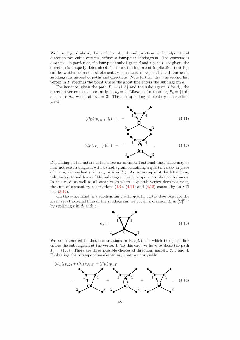
We have argued above, that a choice of path and direction, with endpoint anddirection two cubic vertices, defines a four-point subdiagram. The converse isalso true. In particular, if a four-point subdiagram d and a path P are given, thedirection is uniquely determined. This has the important implication that B43

can be written as a sum of elementary contractions over paths and four-pointsubdiagrams instead of paths and directions. Note further, that the second lastvertex in P specifies the point where the ghost line enters the subdiagram d.

For instance, given the path Ps = 1, 5 and the subdiagram s for ds, thedirection vertex must necessarily be ns = 4. Likewise, for choosing Pu = 1, 6and u for du, we obtain nu = 3. The corresponding elementary contractionsyield

(β43)(Ps,ns)(ds) = −

2 3

1 4(4.11)

(β43)(Pu,nu)(du) = −

2 3

1 4. (4.12)

Depending on the nature of the three uncontracted external lines, there may ormay not exist a diagram with a subdiagram containing a quartic vertex in placeof t in dt (equivalently, s in ds or u in du). As an example of the latter case,take two external lines of the subdiagram to correspond to physical fermions.In this case, as well as all other cases where a quartic vertex does not exist,the sum of elementary contractions (4.9), (4.11) and (4.12) cancels by an STIlike (3.12).

On the other hand, if a subdiagram q with quartic vertex does exist for thegiven set of external lines of the subdiagram, we obtain a diagram dq in [G]ν+1

by replacing t in dt with q:

dq =

2 35

1 4(4.13)

We are interested in those contractions in B44(dq), for which the ghost lineenters the subdiagram at the vertex 1. To this end, we have to chose the pathPq = 1, 5. There are three possible choices of direction, namely, 2, 3 and 4.Evaluating the corresponding elementary contractions yields

(β44)(Pq,2) + (β44)(Pq,3) + (β44)(Pq,4)

=

2 3

1 4+

2 3

1 4+

2 3

1 4. (4.14)

48

This cancels precisely with (4.9), (4.11) and (4.12), just as we anticipated atthe beginning of the section. It is easy to see why there is no difference tothe tree level case in our present example: The four-point subdiagram underconsideration has four distinct external points 1, 2, 3, and 4. Locally, then,there is essentially no difference to the tree level case, if we use a regularizationscheme with shift invariance, like dimensional regularization.

Since the choice of path and subdiagram was arbitrary, our proof is completeonce we can show that, for every choice of four-point subdiagram and path, thecontributions of the elementary contractions β43 and β44 add up with equalweight. For one-loop diagrams, this is a nontrivial assertion, because four-point subdiagrams may have coincident external vertices. When the four-pointsubdiagram is transformed in all possible ways as above, some of the diagramsso obtained may be identical. In this situation, it is not obvious that the gaugecancellations still work as before.

We must now investigate the implications of symmetries which affect thechosen four-point subdiagram d. (If a symmetry does not affect d, since wealways pick diagrams that differ at most in d, the effect of the symmetry canbe at most a global factor.) We begin with the four-point subdiagram q witha quartic vertex, because this subdiagram evidently has the highest symmetry.The three ways to replace q by a subdiagram with a pair of connected cubic ver-tices correspond precisely to the three different ways to group the four externaledges of q in pairs:

e1

e

e3

e2

→

e1

e

e3

e2

⇔ (e, e1)(e2, e3)

,

e1

e

e3

e2

⇔ (e, e2)(e1, e3)

,

e1

e

e3

e2

⇔ (e, e3)(e1, e2)

(4.15)

In fact, the edge e is distinguished because it is part of the path leading to thequartic vertex. Therefore, it actually suffices to specify the second member ofthe pair containing e or, equivalently, the second pair.

Now consider applying the elementary contraction β44 to q. According tothe STI (3.11), we get a sum of three diagrams with an effective BRST vertex:

e1 e3

e2

= −

e1 e3

e2

−

e1 e3

e2

−

e1 e3

e2

(4.16)

Inside a larger diagram, the three diagrams with effective BRST vertex cor-respond to three elementary contractions with the same path but different di-rections. Evidently, these directions can be characterized by the same pairingsof edges as the three subdiagram topologies above. Therefore, the relevantsymmetries of the four-point subdiagram are automorphisms of the three undis-tinguished edges. Furthermore, an elementary contraction characterized by the

49

pair (e, ek) will automatically have the same symmetries as the correspondingfour-point subdiagram.

At one-loop level, there are only two such automorphisms. On one hand,two edges may connect to the same vertex:

Vq = (4.17)

On the other hand, two edges may actually coincide:2

Sq = (4.18)

When the quartic vertex in Vq and Sq is expanded, the edge automorphism ofthe subdiagram can be either preserved or spoiled. In the latter case, due to theautomorphism of the original diagram, there must be different pairings leadingto the same expanded diagram. All this can clearly be seen in the expansionsof Vq and Sq:

Vq → Vs, Vt, Vu =

, ,

(4.19)

Sq → Ss, St, Su =

, ,

(4.20)

Vs and Ss have the same automorphism as Vq and Sq. Vt and Vu are identicalbecause Vq is invariant under a permutation of the two edges which connect tothe same vertex. A similar argument explains the equality of St and Su. In thiscase, however, the resultant subdiagrams still have an automorphism.

Now we have to evaluate the contractions of these diagrams and look whethersymmetry factors are global ones. First, consider the vertex diagrams:

12β44(Vq) =

12

= −12

− (4.21)

12β43(Vs) =

12

=12

(4.22)

β43(Vt) = = (4.23)

2The symbols V and S stand for “vertex” and “self energy”.

50

The sum of all contributions cancels. Since Vt = Vu, we could write this in amore symmetric way as follows:

12β44(Vq) +

12β43(Vs) + β43(Vt) =

12(β44(Vq) + β43(Vs) + β43(Vt) + β43(Vu)

).

(4.24)We see that the symmetry factor has turned into a common prefactor.

In a similar way, we get for the contractions of the self energy diagrams Sq

and Ss:

12β44(Sq) =

12

= −12

− (4.25)

12β43(Ss) =

12

=12

(4.26)

To evaluate the contraction of Vt, we must be a little more precise about thedefinition of elementary contractions. Actually, the elementary contractionsconsidered here should be contractions of diagrams, hence carry a direction. Inthe previous cases the direction was always clear, so we could safely omit it.Now, however, there are two choices:

12

=12

+12

= (4.27)

Both choices lead to equal diagrams. The reason is the same symmetry underpermutation of edges that led to the coefficient of unity in (4.27). Again, wecan use St = Su to turn the symmetry factor into a common prefactor:

12(β44(Sq) + β43(Ss) + 2β43(St)

)=

12(β44(Sq) + β43(Ss) + β43(St) + β43(Su)

)(4.28)

On the other hand, in both cases the potential problems with the symmetryfactors produced by automorphisms were resolved again through these auto-morphisms. As we shall see when we investigate the multi-loop case, this is ageneral scheme.

The demonstration of the cancellations in the four-point subdiagrams withnontrivial symmetry factors completes the proof of (4.6). We emphasize that,in order to produce the cancellations we do not have to match diagrams in [G]ν

and [G]ν+1, which is in general impossible because four-point subdiagrams canoverlap. Rather, we need only match diagrams in B43

([G]ν

)and B44

([G]ν+1) to

make sure that the required gauge cancellations take place. This works becausethe contractions B43 and B44 produce separate additive contributions for everypossible choice of four-point subdiagram. Thereby, overlapping subdiagrams aredisentangled.

Pictorially speaking, B43

([G]ν

)and B44

([G]ν+1) each produce a pile of dia-

grams with effective BRST vertex. These can be sorted according to the subdia-grams that contain the effective BRST vertex. It then turns out that both piles

51

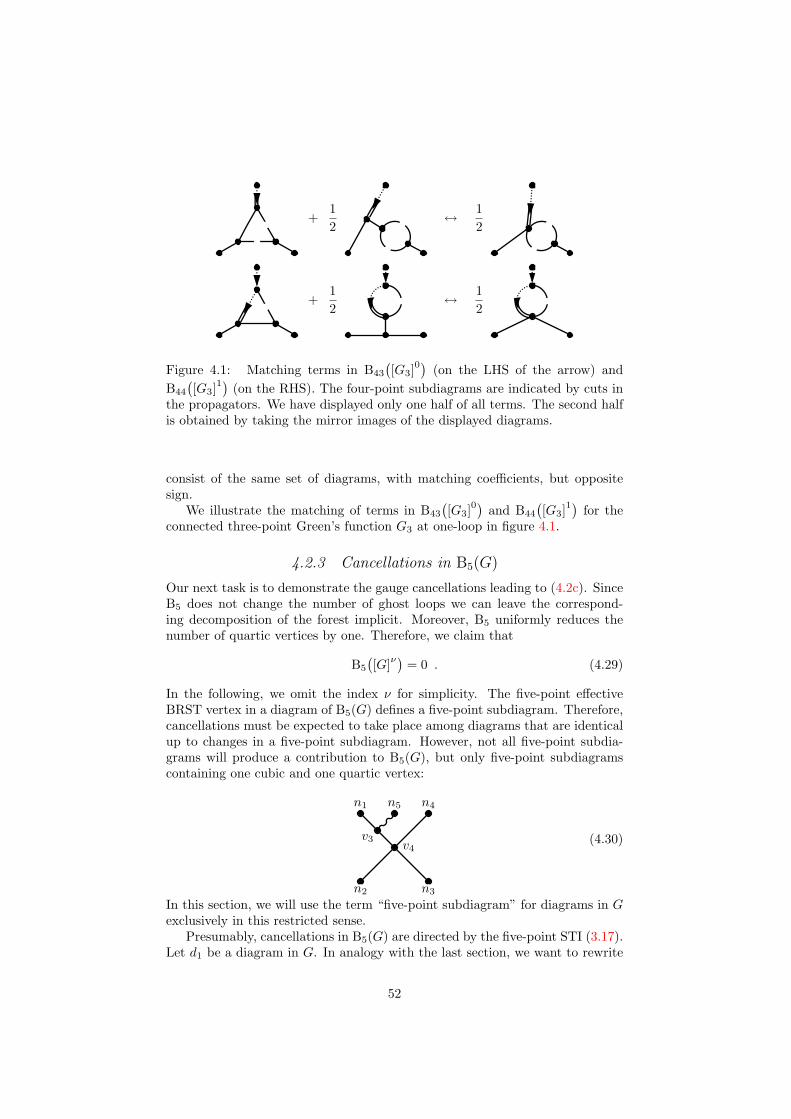
+12

↔ 12

+12

↔ 12

Figure 4.1: Matching terms in B43

([G3]

0) (on the LHS of the arrow) andB44

([G3]

1) (on the RHS). The four-point subdiagrams are indicated by cuts inthe propagators. We have displayed only one half of all terms. The second halfis obtained by taking the mirror images of the displayed diagrams.

consist of the same set of diagrams, with matching coefficients, but oppositesign.

We illustrate the matching of terms in B43

([G3]

0) and B44

([G3]

1) for theconnected three-point Green’s function G3 at one-loop in figure 4.1.

4.2.3 Cancellations in B5(G)

Our next task is to demonstrate the gauge cancellations leading to (4.2c). SinceB5 does not change the number of ghost loops we can leave the correspond-ing decomposition of the forest implicit. Moreover, B5 uniformly reduces thenumber of quartic vertices by one. Therefore, we claim that

B5

([G]ν

)= 0 . (4.29)

In the following, we omit the index ν for simplicity. The five-point effectiveBRST vertex in a diagram of B5(G) defines a five-point subdiagram. Therefore,cancellations must be expected to take place among diagrams that are identicalup to changes in a five-point subdiagram. However, not all five-point subdia-grams will produce a contribution to B5(G), but only five-point subdiagramscontaining one cubic and one quartic vertex:

n2

n1

n3

n4

v4

n5

v3 (4.30)

In this section, we will use the term “five-point subdiagram” for diagrams in Gexclusively in this restricted sense.

Presumably, cancellations in B5(G) are directed by the five-point STI (3.17).Let d1 be a diagram in G. In analogy with the last section, we want to rewrite

52

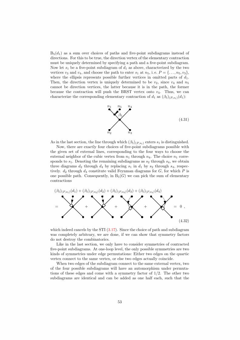
B5(d1) as a sum over choices of paths and five-point subdiagrams instead ofdirections. For this to be true, the direction vertex of the elementary contractionmust be uniquely determined by specifying a path and a five-point subdiagram.Now let s1 be a five-point subdiagram of d1 as above, characterized by the twovertices v3 and v4, and choose the path to enter s1 at n5, i. e. P = . . . , n5, v3,where the ellipsis represents possible further vertices in omitted parts of d1.Then, the direction vertex is uniquely determined to be v2, since v4 and n5

cannot be direction vertices, the latter because it is in the path, the formerbecause the contraction will push the BRST vertex onto v4. Thus, we cancharacterize the corresponding elementary contraction of d1 as (β5)(P,s1)(d1):

β5

n2

n1

n3

n4n5

(4.31)

As in the last section, the line through which (β5)(P,s1) enters s1 is distinguished.Now, there are exactly four choices of five-point subdiagrams possible with

the given set of external lines, corresponding to the four ways to choose theexternal neighbor of the cubic vertex from n1 through n4. The choice n1 corre-sponds to s1. Denoting the remaining subdiagrams as s2 through s4, we obtainthree diagrams d2 through d4 by replacing s1 in d1 by s2 through s4, respec-tively. d2 through d4 constitute valid Feynman diagrams for G, for which P isone possible path. Consequently, in B5(G) we can pick the sum of elementarycontractions

(β5)(P,s1)(d1) + (β5)(P,s2)(d2) + (β5)(P,s3)(d3) + (β5)(P,s4)(d4)

= + + + = 0 ,

(4.32)

which indeed cancels by the STI (3.17). Since the choice of path and subdiagramwas completely arbitrary, we are done, if we can show that symmetry factorsdo not destroy the combinatorics.

Like in the last section, we only have to consider symmetries of contractedfive-point subdiagrams. At one-loop level, the only possible symmetries are twokinds of symmetries under edge permutations: Either two edges on the quarticvertex connect to the same vertex, or else two edges actually coincide.

When two edges of the subdiagram connect to the same external vertex, twoof the four possible subdiagrams will have an automorphism under permuta-tions of these edges and come with a symmetry factor of 1/2. The other twosubdiagrams are identical and can be added as one half each, such that the

53

symmetry factor turns into a global prefactor:

12

+12

+

=12

+ + +

= 0

(4.33)

In the second case, two of four subdiagrams have a tadpole edge and come withsymmetry factor 1/2. The other two subdiagrams are identical, having a doubleedge between cubic and quartic vertex, and consequently carry a symmetryfactor 1/2, too. For the latter subdiagrams, the contraction yields two identicalterms, making up for the symmetry factor, such that only a global factor is left:

12

+12

+12

=12

+ + +

= 0

(4.34)

Thus, we have proved (4.29).

4.2.4 Cancellations in Bc(G)

In this section we will demonstrate the cancellation of diagrams with contrac-tions at ghost lines. Since we are presently considering only diagrams withoutexternal ghost lines, it would appear that such contractions can only be gen-erated in diagrams with a ghost loop. This guess is, however, wrong. Indeed,in the one-loop case, we shall find that diagrams without ghost loop providecancellations for diagrams with ghost loop.

In this section, we can leave the decomposition of the forest according tothe number of quartic vertices implicit, because the elementary contraction βc

cannot change this number. On the other hand, the decomposition of G into[G]0 and [G]01 according to the number of ghost loops is essential.

First, let us demonstrate how a diagram d in [G]0 can produce a contributionto Bc(G) even though by definition it does not contain a ghost line. To this end,recall that the action of the complete contraction map Θ can be described as a

54

recursive operation: Θ enters d through the contracted external line, performingthe elementary contraction θ at every vertex on its way, and then forking at everycubic vertex in all possible ways. Thereby, Θ replaces each gauge field line bya ghost line. Pictorially speaking, Θ drags a ghost line behind while forkingthrough the d. The action of Bc on d can be described in exactly the same way,with the elementary contraction θ replaced by βc.

Now let dt be a diagram in G with a closed gauge field loop containing onlycubic vertices:

dt =

1

24

5

3(4.35)

If Bc can enter the loop, it will circle the loop until it reaches the entry pointagain. But since Bc drags a ghost line behind, the contraction will now encountera ghost line. This corresponds to an elementary contraction with a path Pt

the endpoint of which is already contained in Pt. For definiteness, we choosePt = 1, 2, 3, 4, 5, 3. For our present purposes, it is convenient to split Pt into asubpath P = 1, 2, 3, connecting the start point of the path to the entry pointinto the loop, and a subpath Lt = 4, 5, 3, passing through the loop. Denotingcomposition of subpaths by P Lt, the corresponding elementary contraction(βc)Pt

reads:3

(βc)Pt(dt) = −βc

1

24

5

3(4.36)

(The minus sign is the obligatory one from (3.23).) As the tree level examplein section 3.4 suggests, a diagram in Bc(G) with an elementary contraction at aghost line must be combined with a similar diagram, producing a ghost BRSTvertex according to the STI (3.8) (or, equivalently, (3.26)).

From the above example, it is clear that a matching diagram can alwaysbe found in Bc

([G]1

), i. e. among the contributions of diagrams with one ghost

loop. In particular, replace the loop in dt by a ghost loop, choosing the directionof the ghost arrow identical to that in (βc)Pt

(dt), to obtain a diagram ct in [G]1:

ct =

1

24

5

3(4.37)

The subpath P is a valid path for an elementary contraction in Bc(ct). Evalu-

3Remember that no direction needs to be specified if βc is applied directly at a ghost line.

55

ating this contraction yields

(βc)P (ct) = −βc

1

24

5

3. (4.38)

Adding both contributions using (3.26) we get, remembering to add the minussign for the fermion loop,

(βc)PLt(dt)− (βc)P (ct) =

1

23

5

. (4.39)

The effective BRST vertex in this diagram defines a four-point subdiagram,together with a direction. Presumably, a cancellation will take place with twoother contributions to Bc(G) according to the STI (3.14). Therefore, we haveto look whether such contributions can be found.

Go back to the original diagram dt. Consider the four-point subdiagramdefined by the vertices 3 and 4. These vertices are actually uniquely determinedby the path Pt, as entry point into the loop and its successor, respectively.Transform this subdiagram as follows to obtain a diagram du:

1

23

54 (4.40)

In Bc(du), we can find an elementary contraction with path P Lu, Lu =3, 5, 4:

(βc)PLu(du) = −

1

23

5

(4.41)

Evidently, the ghost effective BRST vertex is contained in the same four-pointsubdiagram as the one in (4.39). Since, in addition, the path P to the subdia-gram is the same in both diagrams, we have found the first of the two matchingcontributions.

The second one should be the same as (4.41) except for an interchange ofthe two incoming ghost lines at the BRST vertex. This elementary contractioncan be found in Bc(cs), where

cs =

1

2

3

4

5

. (4.42)

56

Observe that cs can be obtained from ct by a transformation of the four-pointsubdiagram defined by the vertices 3 and 4, which are again uniquely determinedby the path Pt.

The desired elementary contraction in Bc(cs) is obtained by choosing thepath P :

(βc)P (cs) = −

1

23

5

(4.43)

Adding up all contributions, with appropriate fermion loop signs, we get acomplete cancellation:

(βc)PLt(dt)− (βc)P (ct) + (βc)PLu

(du)− (βc)P (cs) = 0 (4.44)

It may seem that the indicated cancellation depends on the properties of thechosen example diagram. This is, however, not the case. With one exception,to be treated in a moment, the above proof covers the general one-loop case.To see this, first note that all changes in the diagrams are confined to a singlefour-point subdiagram. All parts of the diagrams outside this subdiagram werecompletely arbitrary and did not change at all. Also, the number of vertices inthe loop was (almost) not essential. Indeed, we could have added any numberof vertices to the loop in almost all places without affecting the proof. The onlynecessary constraint is, that the vertices 3 and 4 have to be neighbors. But ifthey were not, 3 and 4 could by no means be contracted into an effective BRSTvertex anyway.

There is, however, one point we have to be careful about. In particular,observe that the diagram cs in the above example has one vertex less in theloop than dt, du and ct. Since this will be the case for any number of verticesin the loop, this opens the possibility that there are unmatched contributionsfor the maximum and minimum possible numbers.

Concerning the maximum possible number of vertices, observe that, if thepath P contains only the external line, no diagram of the form (4.43) is actuallyproduced. To see this, consider the following example:

βc1

24

3−

βc12

4

3(4.45)

When the two contractions are combined like in (4.39), they will contributeto a cancellation among diagrams in Bc(G) with two ghost propagators in theloop, not three. In fact, there is no diagram at all in Bc(G) with three ghostpropagators. Now observe that the number of vertices in the loop is actuallyirrelevant for this argument, which depends only on the fact that the subpathP from the external contraction to the loop is a trivial path consisting of justa single external line. Therefore, we may conclude that no unmatched contri-butions remain for one-loop diagrams with the maximum possible number ofvertices in the loop.

57

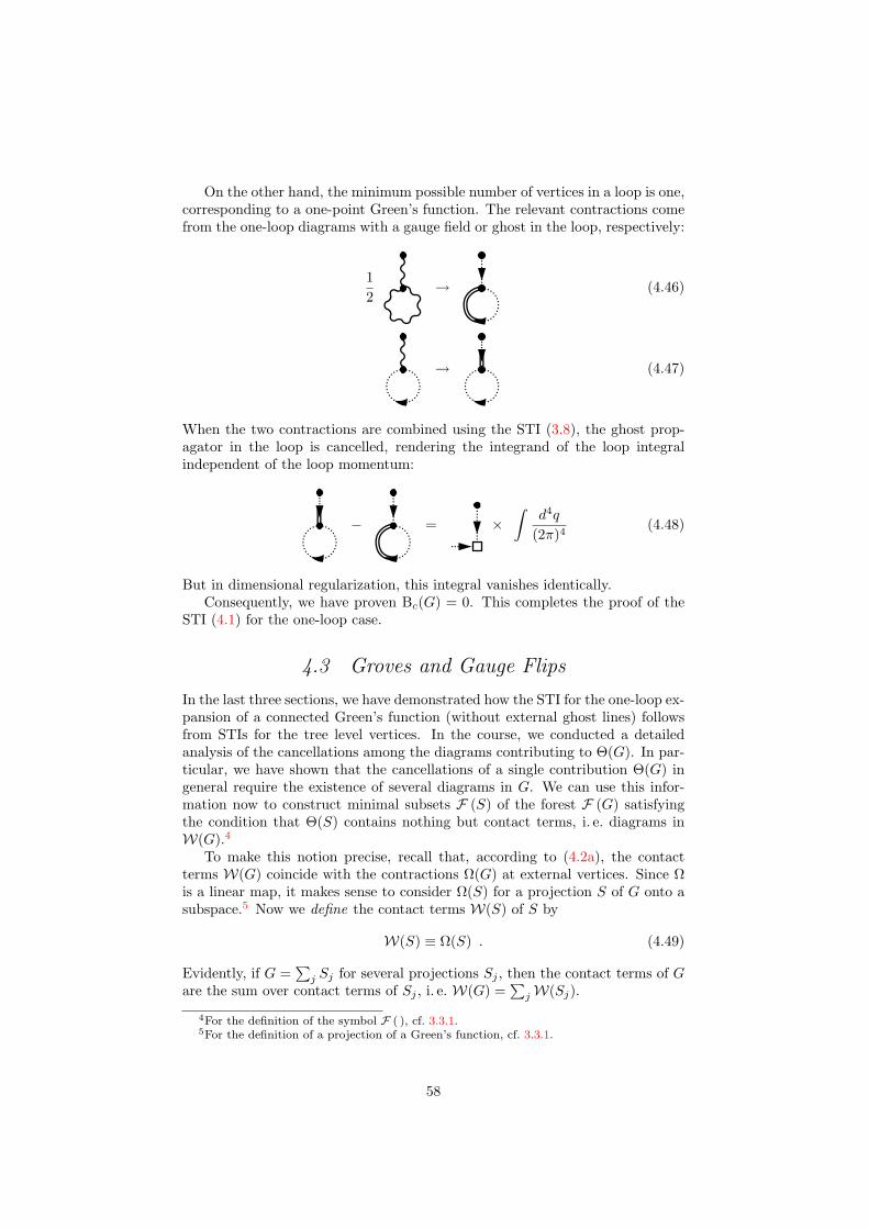
On the other hand, the minimum possible number of vertices in a loop is one,corresponding to a one-point Green’s function. The relevant contractions comefrom the one-loop diagrams with a gauge field or ghost in the loop, respectively:

12

→ (4.46)

→ (4.47)

When the two contractions are combined using the STI (3.8), the ghost prop-agator in the loop is cancelled, rendering the integrand of the loop integralindependent of the loop momentum:

− = ×∫

d4q

(2π)4(4.48)

But in dimensional regularization, this integral vanishes identically.Consequently, we have proven Bc(G) = 0. This completes the proof of the

STI (4.1) for the one-loop case.

4.3 Groves and Gauge Flips

In the last three sections, we have demonstrated how the STI for the one-loop ex-pansion of a connected Green’s function (without external ghost lines) followsfrom STIs for the tree level vertices. In the course, we conducted a detailedanalysis of the cancellations among the diagrams contributing to Θ(G). In par-ticular, we have shown that the cancellations of a single contribution Θ(G) ingeneral require the existence of several diagrams in G. We can use this infor-mation now to construct minimal subsets F (S) of the forest F (G) satisfyingthe condition that Θ(S) contains nothing but contact terms, i. e. diagrams inW(G).4

To make this notion precise, recall that, according to (4.2a), the contactterms W(G) coincide with the contractions Ω(G) at external vertices. Since Ωis a linear map, it makes sense to consider Ω(S) for a projection S of G onto asubspace.5 Now we define the contact terms W(S) of S by

W(S) ≡ Ω(S) . (4.49)

Evidently, if G =∑

j Sj for several projections Sj , then the contact terms of Gare the sum over contact terms of Sj , i. e. W(G) =

∑jW(Sj).

4For the definition of the symbol F ( ), cf. 3.3.1.5For the definition of a projection of a Green’s function, cf. 3.3.1.

58

An invariant subset of the forest F (G) is defined as the set F (S), where Sis a projection of G satisfying

Θ(S) =W(S) . (4.50)

If F (G) is the (disjoint) union of r > 1 invariant subsets F (Sj), this means thatall cancellations required to satisfy the STI for G take place separately withineach invariant subset.

If the Green’s function G has several external gauge boson lines, the con-traction Θ can be applied to each gauge boson line. Denoting by Θ`(G) thecontraction of G at the `-th gauge boson line and by W`(G) the correspondingcontact terms, we must then extend the definition of an invariant subset S toinclude all possible contractions:

Θ`(S) =W`(S) for all ` (4.51)

In the following, (4.50) is always understood in this sense, so we will continueto omit the label for the external gauge boson line.

In analogy to the tree level case [4], we now define the groves of F (G) asthe elements of the finest possible partitioning of F (G) into invariant subsets,which in addition we require to be independent of the gauge parameters, onceonshell matrix elements are extracted from G.6

If F (Gr) is a grove, then no diagram can be omitted from F (Gr) withoutviolating the condition Θ(Gr) =W(Gr) or the gauge parameter independence.It is in this sense, that groves are the minimal gauge invariant classes of Feynmandiagrams.

We are now going to demonstrate that the groves of a connected Green’sfunction G can be constructed by performing graphical operations, called gaugeflips, on Feynman diagrams.

4.3.1 Constructing Groves

To construct a grove, we start with a set F (S) containing a single diagram din the connected Green’s function G. (This means S = χ(d)d.) Applying Θ toS, we get

Θ(S) = Ω(S) + B4(S) + B5(S) + Bc(S) . (4.52)

In general, the B terms will be nonzero. Therefore, in order to satisfy Θ(S) =Ω(S), we must add diagrams of G which provide the necessary cancellations.

First, consider B4(S). According to the discussion in 4.2.2, the requiredcancellations will come from diagrams which differ from d in a single four-pointsubdiagram. Specifically, call a subdiagram with at least one external gaugefield line a gauge subdiagram. A gauge subdiagram which can be reached bya path is denoted as a reachable gauge subdiagram. Remember in this contextthat, by definition, a path always starts at an external line.

We have seen that B4(d) can be written as a sum of elementary contractionsover reachable four-point gauge subdiagrams. Therefore, we have to add to

6The proper framework for the discussion of the gauge parameter dependence of Green’sfunctions is provided by the so-called Nielsen identities [22]. A detailed discussion of thegauge parameter dependence is, however, beyond the scope of this work and therefore left toa separate publication [23]. We give a more intuitive definition here instead.

59

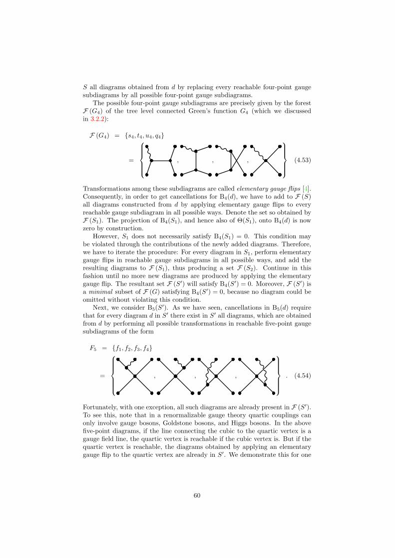
S all diagrams obtained from d by replacing every reachable four-point gaugesubdiagrams by all possible four-point gauge subdiagrams.

The possible four-point gauge subdiagrams are precisely given by the forestF (G4) of the tree level connected Green’s function G4 (which we discussedin 3.2.2):

F (G4) = s4, t4, u4, q4

=

, , ,

(4.53)

Transformations among these subdiagrams are called elementary gauge flips [4].Consequently, in order to get cancellations for B4(d), we have to add to F (S)all diagrams constructed from d by applying elementary gauge flips to everyreachable gauge subdiagram in all possible ways. Denote the set so obtained byF (S1). The projection of B4(S1), and hence also of Θ(S1), onto B4(d) is nowzero by construction.

However, S1 does not necessarily satisfy B4(S1) = 0. This condition maybe violated through the contributions of the newly added diagrams. Therefore,we have to iterate the procedure: For every diagram in S1, perform elementarygauge flips in reachable gauge subdiagrams in all possible ways, and add theresulting diagrams to F (S1), thus producing a set F (S2). Continue in thisfashion until no more new diagrams are produced by applying the elementarygauge flip. The resultant set F (S′) will satisfy B4(S′) = 0. Moreover, F (S′) isa minimal subset of F (G) satisfying B4(S′) = 0, because no diagram could beomitted without violating this condition.

Next, we consider B5(S′). As we have seen, cancellations in B5(d) requirethat for every diagram d in S′ there exist in S′ all diagrams, which are obtainedfrom d by performing all possible transformations in reachable five-point gaugesubdiagrams of the form

F5 = f1, f2, f3, f4

=

, , ,

. (4.54)

Fortunately, with one exception, all such diagrams are already present in F (S′).To see this, note that in a renormalizable gauge theory quartic couplings canonly involve gauge bosons, Goldstone bosons, and Higgs bosons. In the abovefive-point diagrams, if the line connecting the cubic to the quartic vertex is agauge field line, the quartic vertex is reachable if the cubic vertex is. But if thequartic vertex is reachable, the diagrams obtained by applying an elementarygauge flip to the quartic vertex are already in S′. We demonstrate this for one

60

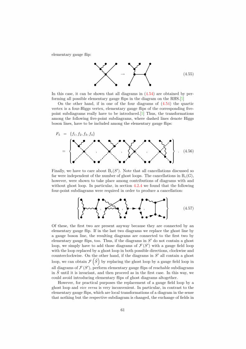
elementary gauge flip:

→ (4.55)

In this case, it can be shown that all diagrams in (4.54) are obtained by per-forming all possible elementary gauge flips in the diagram on the RHS.[5]

On the other hand, if in one of the four diagrams of (4.54) the quarticvertex is a four-Higgs vertex, elementary gauge flips of the corresponding five-point subdiagrams really have to be introduced.[5] Thus, the transformationsamong the following five-point subdiagrams, where dashed lines denote Higgsboson lines, have to be included among the elementary gauge flips:

F5 = f1, f2, f3, f4

=

, , ,

. (4.56)

Finally, we have to care about Bc(S′). Note that all cancellations discussed sofar were independent of the number of ghost loops. The cancellations in Bc(G),however, were shown to take place among contributions of diagrams with andwithout ghost loop. In particular, in section 4.2.4 we found that the followingfour-point subdiagrams were required in order to produce a cancellation: , , ,

(4.57)

Of these, the first two are present anyway because they are connected by anelementary gauge flip. If in the last two diagrams we replace the ghost line bya gauge boson line, the resulting diagrams are connected to the first two byelementary gauge flips, too. Thus, if the diagrams in S′ do not contain a ghostloop, we simply have to add those diagrams of F (S′) with a gauge field loopwith the loop replaced by a ghost loop in both possible directions, clockwise andcounterclockwise. On the other hand, if the diagrams in S′ all contain a ghostloop, we can obtain F

(S)

by replacing the ghost loop by a gauge field loop inall diagrams of F (S′), perform elementary gauge flips of reachable subdiagramsin S until it is invariant, and then proceed as in the first case. In this way, wecould avoid introducing elementary flips of ghost diagrams altogether.

However, for practical purposes the replacement of a gauge field loop by aghost loop and vice versa is very inconvenient. In particular, in contrast to theelementary gauge flips, which are local transformations of a diagram in the sensethat nothing but the respective subdiagram is changed, the exchange of fields in

61

a loop is not a local operation, because the loop may possibly pass through allvertices of the diagram. It is therefore desirable to reduce the number of loopreplacements in favor of local operations.

This can be achieved by introducing elementary gauge flips of four-pointgauge subdiagrams with two ghost lines as follows. First, note that a singleloop replacement is unavoidable, or else we could never get a diagram with aghost loop if the diagrams in S′ had none, and vice versa. But once we havetwo matching diagrams with and without ghost loop, all effects of elementarygauge flips in the diagram with the gauge field loop can be simultaneouslytransferred to the diagram with the ghost loop by defining elementary gaugeflips as transformations among the following four-point gauge subdiagrams:

F (G12) = s12, t12, u12 =

, ,

(4.58)

Observe that, as indicated, this is just the forest F (G12) of the tree level two-ghost connected Green’s function, for which we proved the STI in 3.4. Thus,this definition of elementary ghost gauge flips is consistent with the verificationof STIs for tree level connected Green’s functions with external ghost lines.Similar to the case of the tree level STI for G12, we do not need a flip of afour-point subdiagram with four external ghost lines in the proof of the ghostcancellations (4.2d).

Let us summarize what we have shown. Given a diagram d in G, the min-imal invariant subset S of G containing d can be constructed by the followingprocedure: Initially, take S = d. Then, add to S all diagrams obtained fromd by applying elementary gauge flips, as defined in (4.53), (4.56), and (4.58), inreachable subdiagrams. After that, add all diagrams obtained from diagrams inS by replacing a ghost loop with a gauge field loop and vice versa. This step isnecessary, because a gauge field loop containing a quartic vertex becomes repla-cable by a ghost loop if the quartic vertex is eliminated through an elementarygauge flip. Repeat this process until no more new diagrams are created by eitherelementary gauge flips or replacements.

We would now like to conclude that, apart from the necessary replacementsof a ghost loop by a gauge field loop, and vice versa, the groves of G can be foundby repeatedly applying gauge flips to every diagram in S in all possible ways,until no more new diagrams are found. A gauge flip of a diagram is defined asthe operation of applying an elementary gauge flip to an arbitrary four-pointgauge subdiagram. On the other hand, the proof of the STI (4.1) does onlyrequire that we include elementary gauge flips of reachable four-point gaugesubdiagrams. Thus, in principle the invariant subsets constructed by applyingall gauge flips to S may not be minimal invariant subsets, through the inclusionof elementary gauge flips in non-reachable subdiagrams.

To provide a concrete example of how this might happen, consider the fol-

62

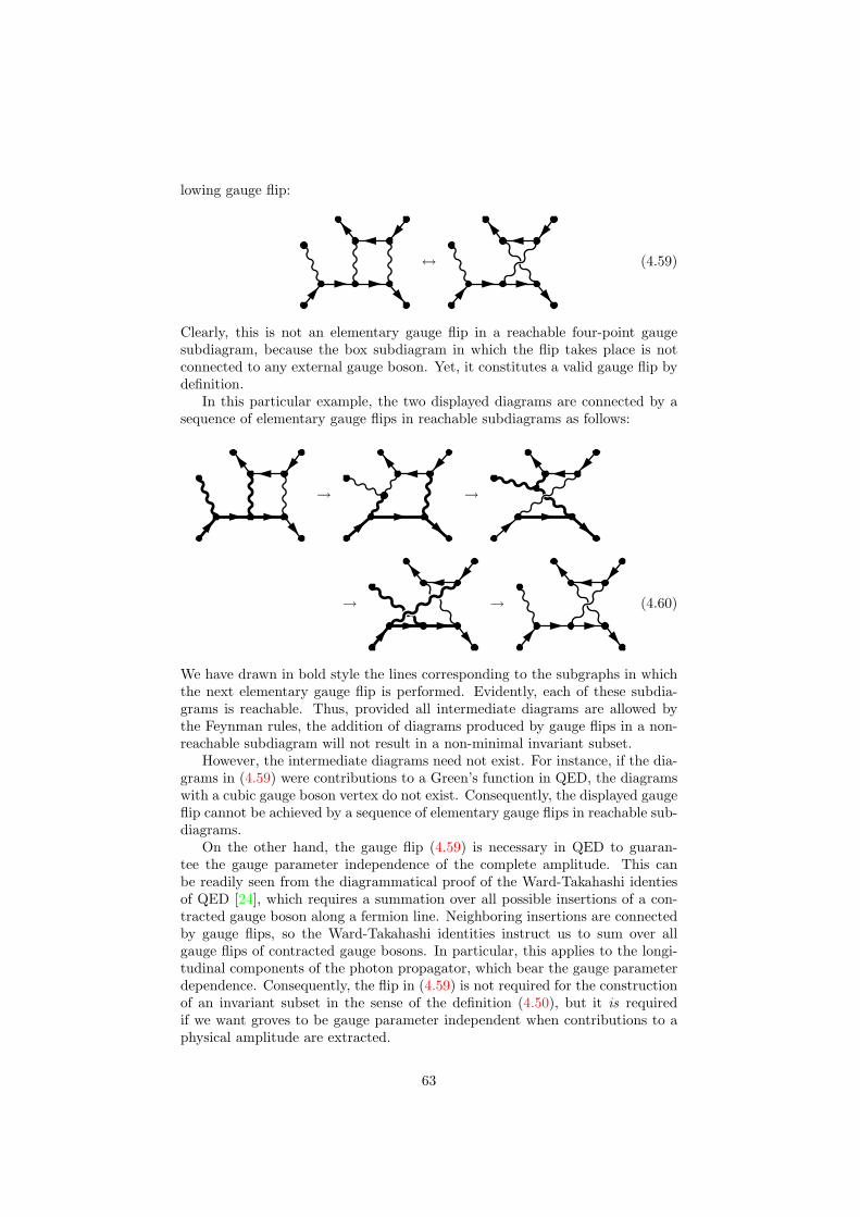
lowing gauge flip:

↔ (4.59)

Clearly, this is not an elementary gauge flip in a reachable four-point gaugesubdiagram, because the box subdiagram in which the flip takes place is notconnected to any external gauge boson. Yet, it constitutes a valid gauge flip bydefinition.

In this particular example, the two displayed diagrams are connected by asequence of elementary gauge flips in reachable subdiagrams as follows:

→ →

→ → (4.60)

We have drawn in bold style the lines corresponding to the subgraphs in whichthe next elementary gauge flip is performed. Evidently, each of these subdia-grams is reachable. Thus, provided all intermediate diagrams are allowed bythe Feynman rules, the addition of diagrams produced by gauge flips in a non-reachable subdiagram will not result in a non-minimal invariant subset.

However, the intermediate diagrams need not exist. For instance, if the dia-grams in (4.59) were contributions to a Green’s function in QED, the diagramswith a cubic gauge boson vertex do not exist. Consequently, the displayed gaugeflip cannot be achieved by a sequence of elementary gauge flips in reachable sub-diagrams.

On the other hand, the gauge flip (4.59) is necessary in QED to guaran-tee the gauge parameter independence of the complete amplitude. This canbe readily seen from the diagrammatical proof of the Ward-Takahashi identiesof QED [24], which requires a summation over all possible insertions of a con-tracted gauge boson along a fermion line. Neighboring insertions are connectedby gauge flips, so the Ward-Takahashi identities instruct us to sum over allgauge flips of contracted gauge bosons. In particular, this applies to the longi-tudinal components of the photon propagator, which bear the gauge parameterdependence. Consequently, the flip in (4.59) is not required for the constructionof an invariant subset in the sense of the definition (4.50), but it is requiredif we want groves to be gauge parameter independent when contributions to aphysical amplitude are extracted.

63

For the case of a general non-abelian gauge theory, broken or unbroken, thisresult has also been proven for the tree level case [5]. Its extension to the one-loop or multi-loop order will be discussed in [5]. In any event, we shall take thegroves of G from now on to denote the equivalence classes of G under sequencesof gauge flips, i. e. two diagrams d and d′ in G belong to the same grove if andonly if d′ can be obtained by successively applying a sequence of gauge flipsto d, and vice versa. With this definition, groves are always invariant subsets,because the elementary gauge flips in reachable subdiagrams are a subset of allpossible gauge flips.

In the next section, when we extend the above proof of the STI (4.1) to themulti-loop case, it will be seen that no new elementary gauge flips have to beintroduced in order to satisfy the STI. Therefore, the set of elementary gaugeflips is already the complete set even in the multi-loop case.

4.4 STI at n-loop

When we proved the general STI (4.1) at one-loop level in (4.2), only some ofour arguments depended on the fact that the diagrams in the Green’s functionG contained exactly one loop. Thus, in order to generalize to the multi-loopcase, we do not need to repeat the complete proof.

However, we shall organize the generalization in the same way as we orga-nized the proof in the one-loop case. We claim that, in the multi-loop case, theproduction of contact terms and the gauge cancellations can still be separatedinto the statements of (4.2). We are now going to consider each statementin turn, indicating the modifications required to transfer the proof from theone-loop case to the multi-loop case.

4.4.1 Production of Contact Terms

The proof of the statement (4.2a) was based on the observations that all dia-grams produced by the elementary contraction ω (cf. (3.55)) are in W(G), andthat, conversely, every diagram in W(G) was given as the elementary contrac-tion ω of a diagram in G. These statements are clearly true in the multi-loopcase, too. Therefore, like in the one-loop case, we only have to worry aboutsymmetry factors.

For one-loop diagrams, there was only one potential source for a mismatchof symmetry factors, which we could easily treat explicitely. In the multi-loopcase, we can no longer treat all possible cases by exhaustion. Rather, we haveto provide general arguments. However, to keep our discussion concrete, we willillustrate our arguments on specific examples. For simplicity, we shall chooseour examples from a pure Yang-Mills theory, drawing gauge bosons as straightlines for ease of notation. None of our arguments will depend on this choice.

Relation (4.2a) can be written, using the definition of elementary contrac-tions of diagrams, as

Ω(G) =∑P(d)

χ(d)ωP (d) =∑

F(W(G))

χ(c)c =W(G) . (4.61)

We know already that both sums are linear combinations of the same set ofdiagrams. We now have to show that, if c is contained in ωP (d) (in the set

64

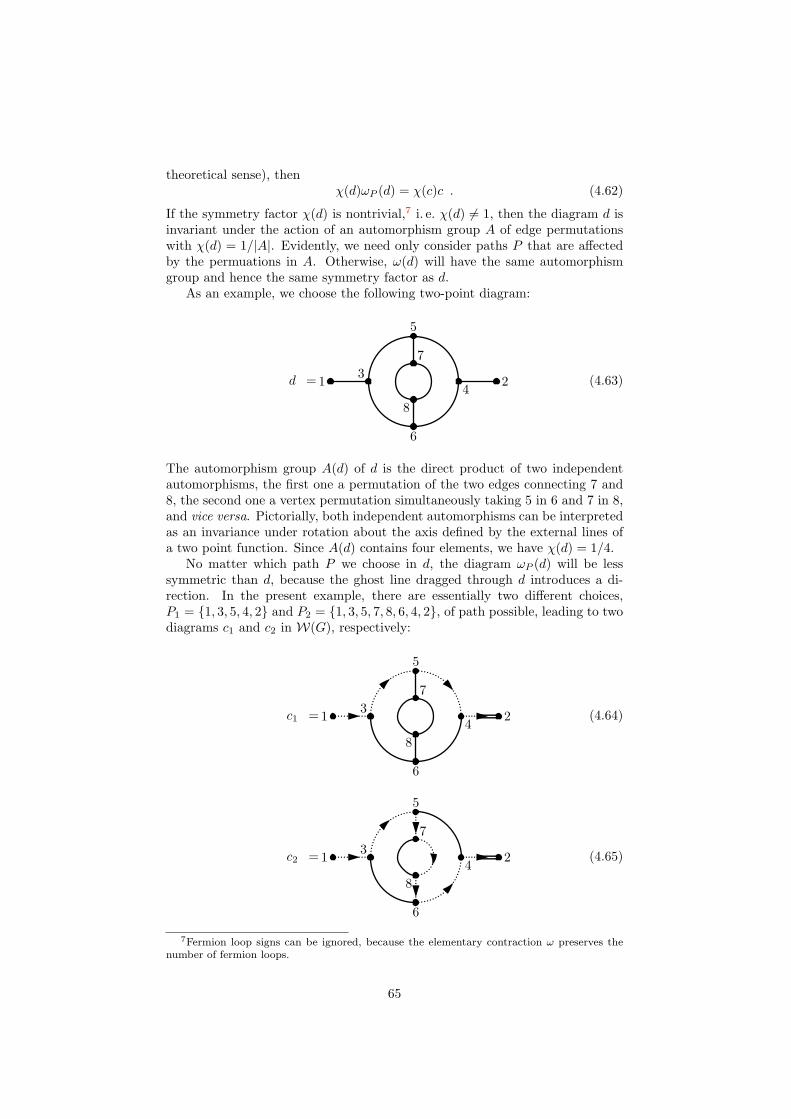
theoretical sense), thenχ(d)ωP (d) = χ(c)c . (4.62)

If the symmetry factor χ(d) is nontrivial,7 i. e. χ(d) 6= 1, then the diagram d isinvariant under the action of an automorphism group A of edge permutationswith χ(d) = 1/|A|. Evidently, we need only consider paths P that are affectedby the permuations in A. Otherwise, ω(d) will have the same automorphismgroup and hence the same symmetry factor as d.

As an example, we choose the following two-point diagram:

d =1 23

5

4

6

7

8

(4.63)

The automorphism group A(d) of d is the direct product of two independentautomorphisms, the first one a permutation of the two edges connecting 7 and8, the second one a vertex permutation simultaneously taking 5 in 6 and 7 in 8,and vice versa. Pictorially, both independent automorphisms can be interpretedas an invariance under rotation about the axis defined by the external lines ofa two point function. Since A(d) contains four elements, we have χ(d) = 1/4.

No matter which path P we choose in d, the diagram ωP (d) will be lesssymmetric than d, because the ghost line dragged through d introduces a di-rection. In the present example, there are essentially two different choices,P1 = 1, 3, 5, 4, 2 and P2 = 1, 3, 5, 7, 8, 6, 4, 2, of path possible, leading to twodiagrams c1 and c2 in W(G), respectively:

c1 =1 23

5

4

6

7

8

(4.64)

c2 =1 23

5

4

6

7

8

(4.65)

7Fermion loop signs can be ignored, because the elementary contraction ω preserves thenumber of fermion loops.

65

c1 is still invariant under the permutation of the double edge, and consequentlyhas χ(c1) = 1/2, while c2 no longer has an automorphism.

Now, consider choosing P ′1 = 1, 3, 6, 4, 2 instead of P1:

c′1 =1 23

5

4

6

7

8

(4.66)

c1 and c′1 are actually identical Feynman diagrams, because one is obtainedfrom the other by a mere index relabeling simultaneously taking 5 in 6 and 7 in8, and vice versa. But this is precisely the action of the original automorphismof d, which has been destroyed by the contraction.

In a similar way, we can find three more paths leading to a diagram identicalto c2:

, ,

(4.67)Again, these are identical Feynman diagrams, once vertex labelings are removed,while the respective vertex labelings are obtained from the one of c2 by applyingthe automorphisms A(d) of the original diagram. Altogether, we get

Ω(d) = χ(d)∑P(d)

ωP (d) =14

(2c1 + 4c2) =12c1+c2 = χ(c1)c1+χ(c2)c2 . (4.68)

Thus, the automorphism ensure that the symmetry factors come out correct inthis example.

This is also true in the general case: Given a diagram d with automorphismgroup A(d) and a path P in d, we can consider the action of the elementarycontraction ωP (d), leading to a contact term diagram c. We say that ωP pre-serves the symmetries corresponding to a subgroup H of A(d), if H is equal tothe automorphism group A(c) of c. In terms of diagrams, this means that thepath P does not pass through the parts of d affected by the automorphisms inH. The remaining automorphisms can be parametrized by the set A(d)/H of(left or right) cosets. Now choose an α in A(d)/H. By definition, α must affectthe path P . Let us denote by Pα the path obtained from P by applying α tothe vertices in P . Then, we have

ωPα(d) = ωP (α(d)) = ωP (d) = c . (4.69)

The coefficient of c in the contact term sum W(G) is given by the sum overelementary contrations and paths that produce c:

66

χ(d)∑

P ′:c∈ωP ′ (d)

ωP ′(d) =1

|A(d)|∑

α∈A(d)/H

ωPα(d)

=1

|A(d)|∑

α∈A(d)/H

ωPα(d) =

1|A(d)|

|A(d)||H|

c =1|H|

c =1

|A(c)|c = χ(c)c (4.70)

This calculation shows that every diagram c in the contact term sum W(G)is produced with the correct weight, proving (4.62), and hence (4.2a), in themulti-loop case.

4.4.2 Cancellations in B4(G) and B5(G)

For the cancellations in B4(G) and B5(G) to work, the contracted four-point orfive-point gauge subdiagrams must come with the correct symmetry factor. Wewould now like to give a general argument that this is always the case.

First, recall that the relevant symmetries are the symmetries of the con-tracted diagrams. These are given as a sum of elementary contractions overpaths and subdiagrams. Consider a particular diagram d in G, as well as apath P and a subdiagram s in d. Denote by H(d, P ) the subgroup of all au-tomorphisms A(d) of d which leaves the path P unaffected. The remainingautomorphisms can be parametrized as in the last section by the set of (leftor right) cosets A(d)/H(d, P ). By an argument identical to the one given inthe last section, the automorphisms affecting the path just make sure that theoriginal symmetry factor 1/|A(d)| is reduced to the factor 1/|H(d, P )|, in ac-cordance with the symmetries remaining when the ghost line has been draggedalong the path P . Now the cancellations in B4(G) and B5(G) take place amongdiagrams that differ only in the subdiagram s, but, in particular, not in the partcontaining P . Therefore, we need only take into account the automorphisms inH(d, P ).

We discuss the cancellations in B4(G) first. For fixed P and four-pointsubdiagram s, consider, as in (4.16), the contraction of the diagram dq in G,which is obtained from d by replacing s with a quartic vertex:

e1 e3

e2

= −

e1 e3

e2

−

e1 e3

e2

−

e1 e3

e2

(4.71)

We display the four-point subdiagram only. It should be understood that thediagram dq extends further, and that some of the displayed edges may coincideor connect to the same vertex.

Denote by K(dq) the subgroup of H(dq) which leaves the edges e1 throughe3 unaffected.8 We must assume that K(dq) is really smaller than H(dq), orelse the symmetry factor 1/|H(dq)| is just a global factor for each of the threediagrams on the RHS of (4.71). The automorphisms in the cosets H(dq)/K(dq)will then necessarily permute one of the edges e1 through e3. However, for thepermutation to be an automorphism, it can at most permute the three edgesamong themselves. (Remember that the edge with the contraction is invariant

8we omit the path argument in H(P, dq), because we consider a fixed path P .

67

under H(dq), because it belongs to the path.) Since the three diagrams witheffective BRST vertex coincide outside the subdiagram s, we have reduced theproblem to the investigation of automorphisms under permutations of the edgese1 through e3.

We can exclude the possibility that two of the three edges coincide, becausethis case has already been treated in section 4.2.2, in the discussion follow-ing (4.16). This leaves only two cases to consider, namely, an automorphismunder permutation of either a pair of edges or all three edges. As an exampleof the former case, consider the following two-loop diagram:

e1 e2

(4.72)

Now, remember that the three elementary contractions on the RHS of (4.71) arecharacterized uniquely by the pair of edges not connected to the effective BRSTvertex. In the present case, if we choose the pair (e1, e2), the correspondingelementary contraction will still be invariant under the automorphism. On theother hand, the two remaining choices lead to identical diagrams, owing tothe action of the automorphism. Therefore, all symmetry factors turn into aglobal prefactor. The argument is really the same as in our discussion of Vq insection 4.2.2, so there’s no need to repeat the details here.

As an example for an invariance under permutation of all three edges, con-sider

. (4.73)

In this case, all three elementary contractions are identical owing to the au-tomorphism, leaving an invariance under permutation of two out of the threeedges. Thus, taking symmetry factors into account, we have

16

= −12

. (4.74)

By the same argument, expanding the quartic vertex in dq into a pair of cubicvertices leads to three identical diagrams with an invariance under permutationof two out of three edges. Evaluating the corresponding contraction yields

12

=12

. (4.75)

Thus, the sum of all contributions cancels. This proves (4.2b) for arbitrarynumbers of loops.

68

For the cancellations in B5(G), we can proceed in an analogous manner. Thesubdiagram s is then a five-point subdiagram as in (4.30), with one out of fiveexternal edges distinguished as lying on the path. The elementary contractionβ5 produces a five-point effective BRST vertex, which singles out one more outof the remaining four edges (cf. (4.32)). Thus, the relevant automorphisms inH/K are those permuting two or three edges at the quartic vertex of the five-point subdiagram. (The case of a tadpole edge, i. e. a pair of coincident edges,has already been treated as a special case in 4.2.3.) If at most two edges arepermuted by the automorphism, the symmetry factors work out exactly as in(4.33).

As an example for the case of three permuted edges, consider the elementarycontraction

16

=16

. (4.76)

Owing to the invariance under permutations of the three symmetric edges atthe quartic vertices, the remaining three elementary contractions, characterizedby connecting one of the symmetric edges to the cubic vertex, are all equal, stillhaving an automorphism under permutation of two out of the symmetric edges:

12

= 3 · 16

(4.77)

Thus, the four elementary contractions contribute with a common factor 1/6,hence cancel according to (4.32). This proves (4.2c) for an arbitrary number ofloops.

4.4.3 Cancellations in Bc(G)

In contrast to the case of cancellations in B4(G) and B5(G), symmetry factorsplay no role for cancellations in Bc(G). This is easily seen from the structure ofthe relevant four-point subgraphs in the STI (3.14): Of the three ghost effectiveBRST vertices, only the one where two incoming ghost lines meet at the BRSTvertex can potentially support a symmetry under edge permutations. However,in our applications there can be no automorphism under permutation of thetwo incoming ghost lines, because one of them will circle a loop, while the otherbegins at an external line. Of course, automorphisms affecting the path mayexist, but these can be treated exactly as in the last two sections. Consequently,we can forget about symmetry factors altogether.

On the other hand, if we consider diagrams with L loops, there are nowdiagrams with any number of ghost loops from 0 to L. Recall that, in the one-loop case, the cancellations took place among diagrams with zero and one ghostloop. In the multi-loop case, we shall now prove that[

Bc

([G]ρ + [G]ρ+1

)]ρ+1

= 0 . (4.78)

69

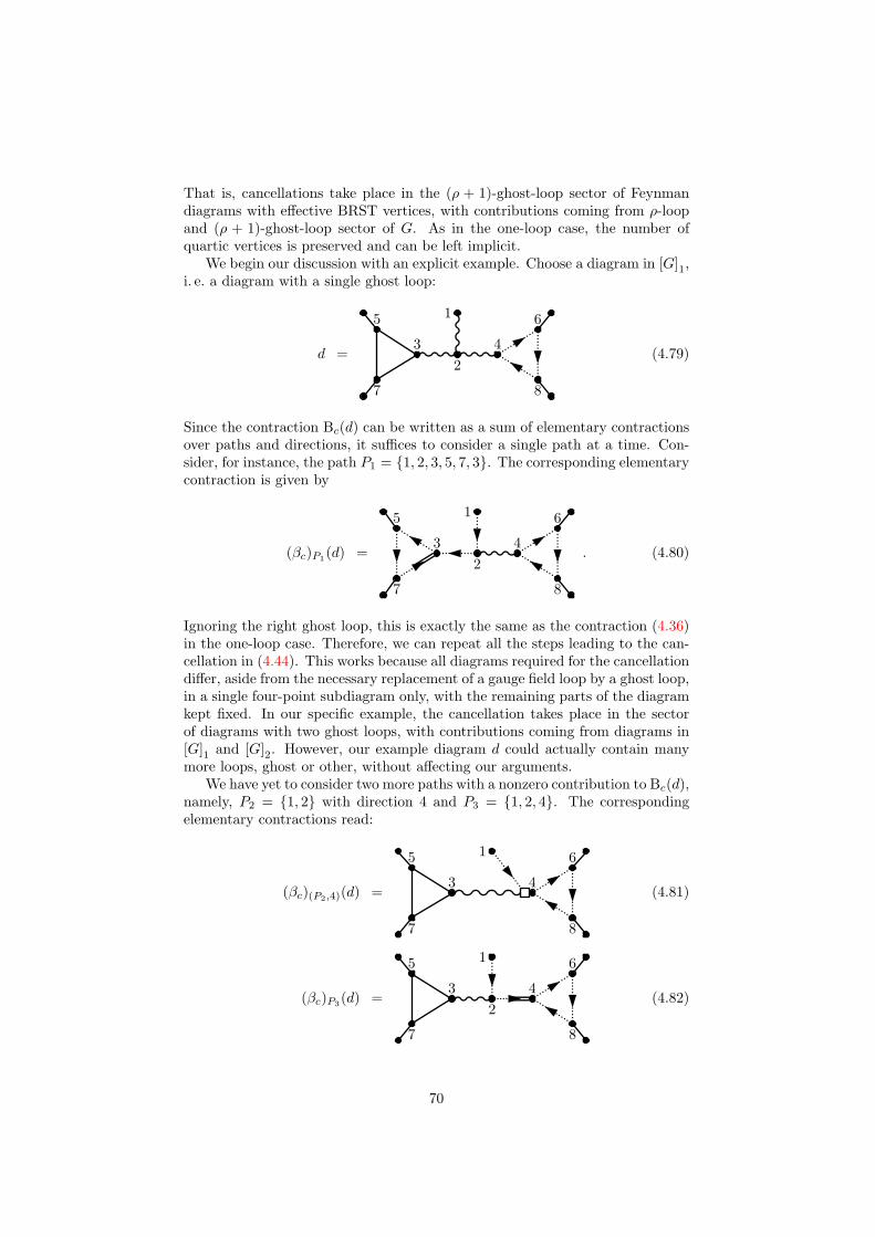
That is, cancellations take place in the (ρ + 1)-ghost-loop sector of Feynmandiagrams with effective BRST vertices, with contributions coming from ρ-loopand (ρ + 1)-ghost-loop sector of G. As in the one-loop case, the number ofquartic vertices is preserved and can be left implicit.

We begin our discussion with an explicit example. Choose a diagram in [G]1,i. e. a diagram with a single ghost loop:

d =

15

7 8

6

3 42

(4.79)

Since the contraction Bc(d) can be written as a sum of elementary contractionsover paths and directions, it suffices to consider a single path at a time. Con-sider, for instance, the path P1 = 1, 2, 3, 5, 7, 3. The corresponding elementarycontraction is given by

(βc)P1(d) =

15

7 8

6

3 42

. (4.80)

Ignoring the right ghost loop, this is exactly the same as the contraction (4.36)in the one-loop case. Therefore, we can repeat all the steps leading to the can-cellation in (4.44). This works because all diagrams required for the cancellationdiffer, aside from the necessary replacement of a gauge field loop by a ghost loop,in a single four-point subdiagram only, with the remaining parts of the diagramkept fixed. In our specific example, the cancellation takes place in the sectorof diagrams with two ghost loops, with contributions coming from diagrams in[G]1 and [G]2. However, our example diagram d could actually contain manymore loops, ghost or other, without affecting our arguments.

We have yet to consider two more paths with a nonzero contribution to Bc(d),namely, P2 = 1, 2 with direction 4 and P3 = 1, 2, 4. The correspondingelementary contractions read:

(βc)(P2,4)(d) =

15

7 8

6

3 4(4.81)

(βc)P3(d) =

15

7 8

6

3 42

(4.82)

70

However, this time we can just ignore the left loop and proceed as in the one-loopcase. The displayed elementary contractions will then combine with elementarycontractions of diagrams in [G]0 without a ghost loop to form a cancellationin the sector of diagrams with a single ghost loop. (Note that (βc)(P2,4)(d)and (βc)P3(d) contribute to different cancellations.) Again, the structure of theunaffected parts of the diagrams is actually arbitrary.

Finally, since cancellations take place among diagrams for which the numberof vertices in the contracted ghost loop differs by one, the cases of ghost loopswith the maximum or minimum possible number of loops can be treated inexactly the same way as in the one-loop case. (Cf. the discussion at the end ofsection 4.2.4.) Concerning cancellations in Bc(G), there is then essentially nodifference between the one-loop diagrams and multi-loop diagrams.

Given the possibility of overlapping gauge field loops, this result might ap-pear a little surprising. Therefore, we will give a further illustration of thecombinatorics of the cancellations. To this end, we consider the action of thecontraction Bc on a diagram d as a recursive map. The contraction is prop-agated into the diagram along gauge field lines, forking at every cubic vertex,dragging a ghost line behind. Nonzero contributions require that the contrac-tion encounters a ghost line. This happens in two ways: The contraction caneither hit a ghost loop, or it can traverse a gauge field loop completely, until ithits the ghost line it dragged behind itself.

The latter case is particularly interesting, because then the contraction in-creases the number of ghost loops by one. To see what this means for the caseof overlapping gauge field loops, suppose d has a two-point subdiagram of theform

. (4.83)

When the contraction propagates into this subdiagram from the left, it willproduce the following elementary contractions: , ,

(4.84)

Evidently, the contraction Bc produces a separate elementary contraction forevery possible choice of a single gauge field loop. But to each choice therecorresponds precisely a diagram with one more ghost loop than d, identical tod up to the displayed two-point subdiagrams: , ,

(4.85)

This property of the contraction Bc generalizes immediately to the case of an ar-bitrary number of overlapping loops: The contraction Bc produces for a diagramd a separate elementary contraction for every possible choice of a traversablegauge field loop in d. Traversable here means that a path circling the loop must

71

exist. Consequently, since the number of ghost loops of d was arbitrary, thereis a correspondence between the elementary contractions with ρ+1 ghost loopsin Bc

([G]ρ

)and the diagrams in [G]ρ+1.

To see how this correspondence can be exploited to simplify the combi-natorics of cancellations in Bc(G), consider the diagrams without ghost loop,i. e. [G]0. Suppose of Bc circles a gauge field loop L0 along path P0 in a diagramd0 in [G]0, producing (βc)P0L0(d0). Then, the corresponding diagram d1 in[G]1 is obtained simply replacing the ghost line leading to L0 in (βc)P0(d0) bythe original gauge field line that was present in d0. The existence of the elemen-tary contraction (βc)P0(d1) is then automatically guaranteed. The existence ofthe other elementary contractions required for the cancellation follows from thediscussion above. Since Bc can do nothing else but pick a ghost loop in [G]0,Bc

([G]0

)is cancelled completely. The same applies to all diagrams with a single

ghost loop in Bc

([G]1

), because these were all required to cancel Bc

([G]0

).

However, we have not yet exhausted the action of Bc on [G]1. In fact, givend1 in [G]1,

9 Bc may circle a gauge field loop L1 along a path P1 in d1. By thesame arguments as before, the existence of matching contributions in Bc

([G]1

)and Bc

([G]2

)can be inferred.

Evidently, we can continue this process up to an arbitrary number ρ of ghostloops. The process will terminate when there is no more gauge field loop thatcould be circled by Bc. Thus, we have proven that the cancellations in Bc takeplace as claimed in (4.78). This completes the proof of the STI (4.1) for anarbitrary number of loops.

4.4.4 Groves and Gauge Flips

Having completed the diagrammatical proof of the STI (4.1) for an arbitrarynumber of loops, we can now extend the notions of groves and gauge flips to themulti-loop case. LetG denote the expansion of a connected Green’s function intoFeynman diagrams at n-loop order. The definition (4.50) of invariant subsets ofthe forest F (G) is taken over unchanged. Also, the groves of F (G) are againthe elements of the finest possible partitioning of F (G) into invariant subsets.

A priori, the cancellations in the multi-loop case could require the introduc-tion of further gauge flips, in addition to the ones constructed for the one-loopcase (cf. 4.3). However, the cancellations in B4(G), B5(G), and Bc(G) still in-volve the same reachable four-point or five-point gauge subdiagrams as in theone-loop case. Indeed, the multi-loop case just introduced additional combina-torial factors, but not new kinds of cancellations. Therefore, we conclude thatthe elementary gauge flips as defined in (4.53), (4.56), and (4.58) constitute thecorrect set of elementary gauge flips for the construction of invariant subsets ofF (G) at an arbitrary order of perturbation theory.

On the other hand, in the multi-loop case we need a more general proce-dure to make sure that diagrams with all possible numbers of ghost loops areproduced. Recall that, if overlapping gauge field loops are present, mutuallyexclusive choices of ghost loops are possible (cf. (4.84)). Therefore, we startfrom a diagram d without ghost loop. (If d contains ghost loops, we just replacethem by gauge field loops.)

9Of course, this d1 is not the same as the one in the last paragraph.

72

Given d without ghost loop, we apply all possible elementary gauge flips inreachable subdiagrams as in the one-loop case. This will produce all requireddiagrams without ghost loop. After that, choose a single diagram without ghostloop and replace an arbitrary gauge field loop by a ghost loop, if there is any.All other required diagrams with a ghost loop are then produced by applyinggauge flips to this single diagram. This is true, because the ghost-gauge bosonsubdiagrams have the same gauge flips as pure gauge boson subdiagrams.

Therefore, in order to construct the diagrams with all possible numbers ofghost loops, we need only repeat the procedure just described: Having addedall gauge flipped diagrams with one ghost loop, we choose a single diagram withone ghost loop and replace some gauge field loop by a second ghost loop. Afterthat, we apply gauge flips again to obtain all diagrams with two ghost loops.This process is continued until the maximum possible number of ghost loops isreached.

Having determined a general procedure for the construction of minimal in-variant subsets of a connected Green’s function G in the multi-loop case, weemphasize again that we have defined groves as the equivalence classes of F (G)under sequences of all gauge flips, not only gauge flips in reachable subdiagrams.Therefore, also in the multi-loop case the groves of F (G) are not necessarily theminimal subsets satisfying (4.50). However, as will be demonstrated in [23], theinclusion of elementary gauge flips in non-reachable subdiagrams is necessary tomake the contribution of a single grove to a physical amplitude gauge parameterindependent.

Before closing this chapter, we remark that, for practical purposes, a differentbut equivalent strategy for the construction of groves may be more efficient.In particular, once we have determined all diagrams without ghost loop, therequired diagrams with n ghost loops can be obtained by replacing, in eachdiagram without ghost loop, n non-overlapping gauge field loops in all possibleways (which, of course, can be done recursively, increasing the number of ghostloops by one in each step). This procedure will lead to the same set of diagramsas the one described above, because the gauge flips performed in the diagramswith ghost loops occur also in the diagrams without a ghost loop.

73

—5—Unflavored Flips

Having described an algorithm for the construction of groves in gauge theories bymeans of gauge flips, as defined in section 4.3, the logical next step would be thatwe apply this algorithm to investigate the forest of connected Green’s functionsin the Standard Model, which is our paradigm for a spontaneously broken gaugetheory. However, flips, when interpreted as graphical operations on Feynmandiagrams, have a meaning independent of the context of gauge theories. Inparticular, they can be used for the construction of Feynman diagrams in generalperturbative quantum field theories with renormalizable interactions. In thischapter, we shall develop a formalism for flips of unflavored diagrams. Weshall derive a number o derive a number of results on the structure of theforest of unflavored n-loop diagrams with certain properties, e. g. 1PI diagramsor amputated diagrams. Gauge theories are then taken up again in the nextchapter.

5.1 Flips Without Flavor: The Basic Tool

In the previous chapter, we have proven that the groves of a connected Green’sfunction at an arbitrary loop order can be constructed by applying gauge flipsto Feynman diagrams, i. e. exchanging a certain four-point gauge subdiagramby another one. Thus, a gauge flip transforms Feynman diagrams into eachother, an operation that can be described in purely graphical terms, where nomore reference to the meaning of a Feynman diagram as a representative for ananalytical expression is made.

We can go even further and detach the notion of flips completely from thecontext of gauge theories. To this end, we forget about the field types, i. e. thequantum numbers, of the lines in a Feynman diagram and consider transforma-tions in an arbitrary four-point subdiagram. That is, we consider the possibletopologies of Feynman diagrams in a general renormalizable gauge theory, andhow they can be transformed into each other by exchanging four-point subdia-grams.

The relevant topologies of Feynman diagrams can easily be generated fromthe Feynman rules corresponding to the theory of a self-interacting real scalarfield with cubic and quartic interactions. Such a theory has no quantum numbersconnected with internal degrees of freedom, and the interaction degrees cover allrenormalizable interactions in non-abelian gauge theories. It can be described

74

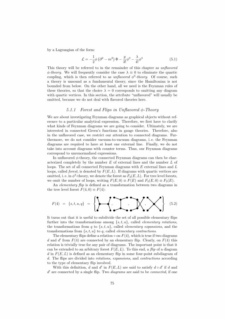
by a Lagrangian of the form:

L = −12φ(∂2 −m2

)Φ− g

3!φ3 − λ

4!φ4 (5.1)

This theory will be referred to in the remainder of this chapter as unflavoredφ-theory. We will frequently consider the case λ ≡ 0 to eliminate the quarticcoupling, which is then referred to as unflavored φ3-theory. Of course, sucha theory is unsound as a fundamental theory, since the Hamiltonian is notbounded from below. On the other hand, all we need is the Feynman rules ofthese theories, so that the choice λ = 0 corresponds to omitting any diagramwith quartic vertices. In this section, the attribute “unflavored” will usually beomitted, because we do not deal with flavored theories here.

5.1.1 Forest and Flips in Unflavored φ-Theory

We are about investigating Feynman diagrams as graphical objects without ref-erence to a particular analytical expression. Therefore, we first have to clarifywhat kinds of Feynman diagrams we are going to consider. Ultimately, we areinterested in connected Green’s functions in gauge theories. Therefore, alsoin the unflavored case, we restrict our attention to connected diagrams. Fur-thermore, we do not consider vacuum-to-vacuum diagrams, i. e. the Feynmandiagrams are required to have at least one external line. Finally, we do nottake into account diagrams with counter terms. Thus, our Feynman diagramscorrespond to unrenormalized expressions.

In unflavored φ-theory, the connected Feynman diagrams can then be char-acterized completely by the number E of external lines and the number L ofloops. The set of all connected Feynman diagrams with E external lines and Lloops, called forest, is denoted by F (E,L). If diagrams with quartic vertices areomitted, i. e. in φ3-theory, we denote the forest as F3(E,L). For tree level forests,we omit the number of loops, writing F (E, 0) ≡ F (E) and F3(E, 0) ≡ F3(E).

An elementary flip is defined as a transformation between two diagrams inthe tree level forest F (4, 0) ≡ F (4):

F (4) = s, t, u, q =

, , ,

(5.2)

It turns out that it is useful to subdivide the set of all possible elementary flipsfurther into the transformations among s, t, u, called elementary rotations,the transformations from q to s, t, u, called elementary expansions, and thetransformations from s, t, u to q, called elementary contractions.

The elementary flips define a relation on F (4), which is true if two diagramsd and d′ from F (4) are connected by an elementary flip. Clearly, on F (4) thisrelation is trivially true for any pair of diagrams. The important point is that itcan be extended to an arbitrary forest F (E,L). To this end, a flip of a diagramd in F (E,L) is defined as an elementary flip in some four-point subdiagram ofd. The flips are divided into rotations, expansions, and contractions accordingto the type of elementary flip involved.

With this definition, d and d′ in F (E,L) are said to satisfy d d′ if d andd′ are connected by a single flip. Two diagrams are said to be connected, if one

75

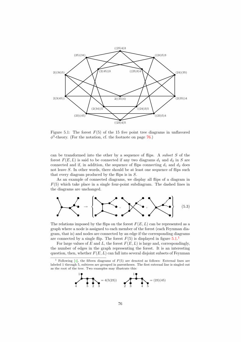
(23)(45)

2(3(45))

2((34)5)

(25)(34)

((25)4)3

((24)5)3

(24)(35)

(2(35))4

((23)5)4

((23)4)5

(2(45))3

(2(34))5

2((35)4)

((24)3)5

((25)3)4

Figure 5.1: The forest F (5) of the 15 five point tree diagrams in unflavoredφ3-theory. (For the notation, cf. the footnote on page 76.)

can be transformed into the other by a sequence of flips. A subset S of theforest F (E,L) is said to be connected if any two diagrams d1 and d2 in S areconnected and if, in addition, the sequence of flips connecting d1 and d2 doesnot leave S. In other words, there should be at least one sequence of flips suchthat every diagram produced by the flips is in S.

As an example of connected diagrams, we display all flips of a diagram inF (5) which take place in a single four-point subdiagram. The dashed lines inthe diagrams are unchanged.

→

, ,

(5.3)

The relations imposed by the flips on the forest F (E,L) can be represented as agraph where a node is assigned to each member of the forest (each Feynman dia-gram, that is) and nodes are connected by an edge if the corresponding diagramsare connected by a single flip. The forest F (5) is displayed in figure 5.1.1

For large values of E and L, the forest F (E,L) is large and, correspondingly,the number of edges in the graph representing the forest. It is an interestingquestion, then, whether F (E,L) can fall into several disjoint subsets of Feynman

1 Following [4], the fifteen diagrams of F (5) are denoted as follows: External lines arelabeled 1 through 5, subtrees are grouped in parentheses. The first external line is singled outas the root of the tree. Two examples may illustrate this:

1

4 5 2 3

= 4(5(23))

1

2 3 4 5

= (23)(45)

76

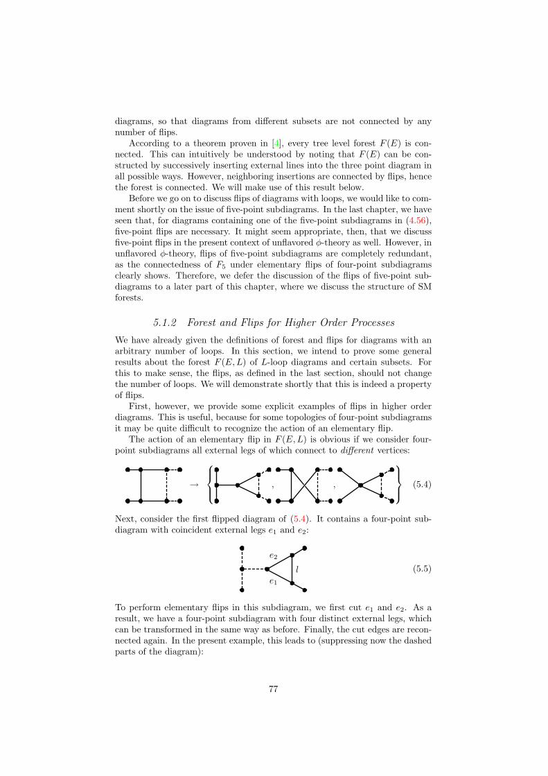
diagrams, so that diagrams from different subsets are not connected by anynumber of flips.

According to a theorem proven in [4], every tree level forest F (E) is con-nected. This can intuitively be understood by noting that F (E) can be con-structed by successively inserting external lines into the three point diagram inall possible ways. However, neighboring insertions are connected by flips, hencethe forest is connected. We will make use of this result below.

Before we go on to discuss flips of diagrams with loops, we would like to com-ment shortly on the issue of five-point subdiagrams. In the last chapter, we haveseen that, for diagrams containing one of the five-point subdiagrams in (4.56),five-point flips are necessary. It might seem appropriate, then, that we discussfive-point flips in the present context of unflavored φ-theory as well. However, inunflavored φ-theory, flips of five-point subdiagrams are completely redundant,as the connectedness of F5 under elementary flips of four-point subdiagramsclearly shows. Therefore, we defer the discussion of the flips of five-point sub-diagrams to a later part of this chapter, where we discuss the structure of SMforests.

5.1.2 Forest and Flips for Higher Order Processes

We have already given the definitions of forest and flips for diagrams with anarbitrary number of loops. In this section, we intend to prove some generalresults about the forest F (E,L) of L-loop diagrams and certain subsets. Forthis to make sense, the flips, as defined in the last section, should not changethe number of loops. We will demonstrate shortly that this is indeed a propertyof flips.

First, however, we provide some explicit examples of flips in higher orderdiagrams. This is useful, because for some topologies of four-point subdiagramsit may be quite difficult to recognize the action of an elementary flip.

The action of an elementary flip in F (E,L) is obvious if we consider four-point subdiagrams all external legs of which connect to different vertices:

→

, ,

(5.4)

Next, consider the first flipped diagram of (5.4). It contains a four-point sub-diagram with coincident external legs e1 and e2:

le1

e2

(5.5)

To perform elementary flips in this subdiagram, we first cut e1 and e2. As aresult, we have a four-point subdiagram with four distinct external legs, whichcan be transformed in the same way as before. Finally, the cut edges are recon-nected again. In the present example, this leads to (suppressing now the dashedparts of the diagram):

77

→

, ,

=

, ,

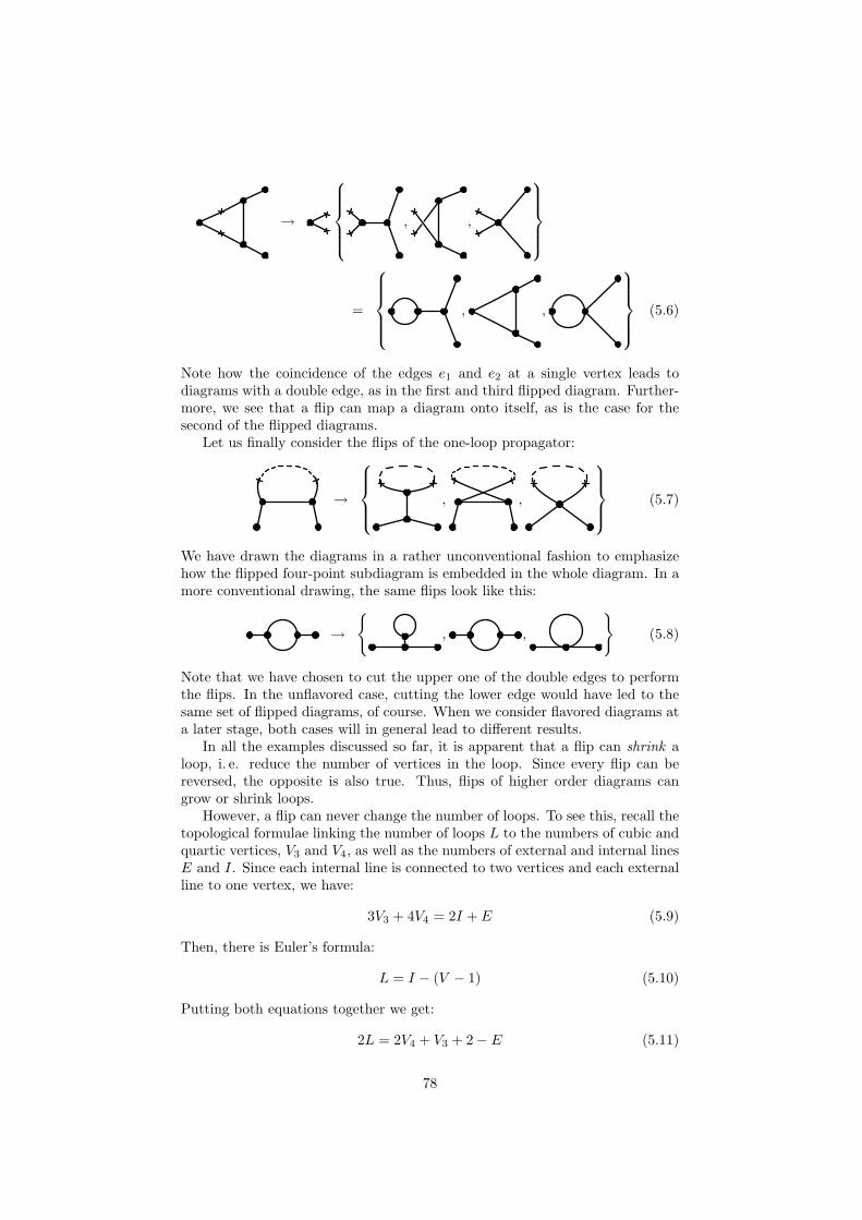
(5.6)

Note how the coincidence of the edges e1 and e2 at a single vertex leads todiagrams with a double edge, as in the first and third flipped diagram. Further-more, we see that a flip can map a diagram onto itself, as is the case for thesecond of the flipped diagrams.

Let us finally consider the flips of the one-loop propagator:

→

, ,

(5.7)

We have drawn the diagrams in a rather unconventional fashion to emphasizehow the flipped four-point subdiagram is embedded in the whole diagram. In amore conventional drawing, the same flips look like this:

→

, ,

(5.8)

Note that we have chosen to cut the upper one of the double edges to performthe flips. In the unflavored case, cutting the lower edge would have led to thesame set of flipped diagrams, of course. When we consider flavored diagrams ata later stage, both cases will in general lead to different results.

In all the examples discussed so far, it is apparent that a flip can shrink aloop, i. e. reduce the number of vertices in the loop. Since every flip can bereversed, the opposite is also true. Thus, flips of higher order diagrams cangrow or shrink loops.

However, a flip can never change the number of loops. To see this, recall thetopological formulae linking the number of loops L to the numbers of cubic andquartic vertices, V3 and V4, as well as the numbers of external and internal linesE and I. Since each internal line is connected to two vertices and each externalline to one vertex, we have:

3V3 + 4V4 = 2I + E (5.9)

Then, there is Euler’s formula:

L = I − (V − 1) (5.10)

Putting both equations together we get:

2L = 2V4 + V3 + 2− E (5.11)

78

Now look a the elementary flips among the diagrams in (5.2). The flips amongs, t, and u just reorganize the given vertices and lines, so they do not changeL. A flip to q decreases V3 by two, I by one and increases V4 by one, whileleaving E invariant. Thus, the number of loops L and therefore the completeforest F (E,L) is invariant under flips.

Since F (E,L) is invariant, it makes sense to ask whether or not it is con-nected. As we shall now prove, it is:

Theorem 5.1 The unflavored forest F (E,L) of connected L-loop diagrams isconnected for any number E of external lines and any number L of loops.

To prove this statement, we note that from a diagram in F (E,L) we can obtaina diagram of the tree level forest F (E + 2L) by cutting L lines. Conversely,from every diagram in F (E + 2L) we can get a diagram in F (E,L) by joining2L external lines. Now take d1 and d2 in F (E,L). First, cut L external linesin d1 and d2 to obtain d′1 and d′2 in F (E + 2L), respectively. Then, d′1 and d′2are connected in F (E + 2L), because all tree level forests are connected. But asequence of flips in F (E + 2L) defines a valid sequence of flips in F (E,L), if wejoin the L cut lines again. Hence F (E,L) is connected, as was to be proved. Ofcourse, there is in general no unique prescription to perform the L cuts. This is,however, not necessary, because we need only demonstrate existence of at leastone sequence of flips connecting d1 and d2.

This result is of practical importance, because it guarantees that the com-plete forest F (E,L) can be produced from a single diagram by repeatedly ap-plying flips. However, at higher orders of perturbation theory, constructing thecomplete forest of diagrams representing a connected Green’s function is notalways desired. For instance, if we are interested in scattering matrix elements,only amputated diagrams must be taken into account. At tree level, there isno difference between amputated and non-amputated diagrams, except for thedifferent interpretation of external lines. For diagrams with loops, on the otherhand, the amputated diagrams are a real subset of the complete forest F (E,L).Also, we may or may not want to include one-point insertions, or we may requirejust the subset of 1PI diagrams.

This means that, in many cases, we will be interested in a subset S of thecomplete forest F (E,L). If we want to produce the diagrams in S by performingflips, starting from a given diagram d in S, it would clearly be advantageous ifwe knew that every diagram in S can be generated from d by a sequence of flipsleading only to diagrams within S. In other words, S should be a connectedsubset. For then we could throw away immediately any flipped diagram whichis not in S.

Of course, an arbitrarily chosen subset of F (E,L) need not necessarily beconnected. In the remainder of this section, we want to study the connectednessof the aforementioned subsets of the complete forest F (E,L). This study can besimplified by demonstrating that the four-point subdiagram q in (5.2) is actuallymeaningless for the connectedness of a forest. This is the reason why we dividedthe flips into rotations on one hand as well as expansions and contractions onthe other hand. (Cf. the definitions below (5.2).)

Now, we can state and prove the connectedness of the forest F3(E,L), whichis the subset of F (E,L) of diagrams without quartic vertices:

79

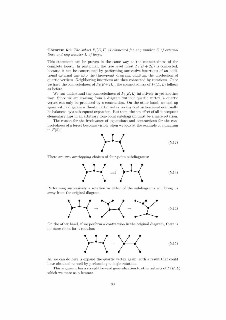
Theorem 5.2 The subset F3(E,L) is connected for any number E of externallines and any number L of loops.

This statement can be proven in the same way as the connectedness of thecomplete forest. In particular, the tree level forest F3(E + 2L) is connected,because it can be constructed by performing successive insertions of an addi-tional external line into the three-point diagram, omitting the production ofquartic vertices. Neighboring insertions are then connected by rotations. Oncewe have the connectedness of F3(E+2L), the connectedness of F3(E,L) followsas before.

We can understand the connectedness of F3(E,L) intuitively in yet anotherway. Since we are starting from a diagram without quartic vertex, a quarticvertex can only be produced by a contraction. On the other hand, we end upagain with a diagram without quartic vertex, so any contraction must eventuallybe balanced by a subsequent expansion. But then, the net effect of all subsequentelementary flips in an arbitrary four-point subdiagram must be a mere rotation.

The reason for the irrelevance of expansions and contractions for the con-nectedness of a forest becomes visible when we look at the example of a diagramin F (5):

(5.12)

There are two overlapping choices of four-point subdiagrams:

and (5.13)

Performing successively a rotation in either of the subdiagrams will bring usaway from the original diagram:

→ → (5.14)

On the other hand, if we perform a contraction in the original diagram, there isno more room for a rotation:

→ (5.15)

All we can do here is expand the quartic vertex again, with a result that couldhave obtained as well by performing a single rotation.

This argument has a straightforward generalization to other subsets of F (E,L),which we state as a lemma:

80

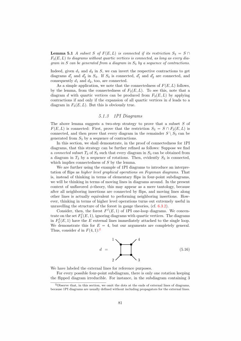
Lemma 5.1 A subset S of F (E,L) is connected if its restriction S3 = S ∩F3(E,L) to diagrams without quartic vertices is connected, as long as every dia-gram in S can be generated from a diagram in S3 by a sequence of contractions.

Indeed, given d1 and d2 in S, we can invert the respective contractions to getdiagrams d′1 and d′2 in S3. If S3 is connected, d′1 and d′2 are connected, andconsequently d1 and d2, too, are connected.

As a simple application, we note that the connectedness of F (E,L) follows,by the lemma, from the connectedness of F3(E,L). To see this, note that adiagram d with quartic vertices can be produced from F3(E,L) by applyingcontractions if and only if the expansion of all quartic vertices in d leads to adiagram in F3(E,L). But this is obviously true.

5.1.3 1PI Diagrams

The above lemma suggests a two-step strategy to prove that a subset S ofF (E,L) is connected: First, prove that the restriction S3 = S ∩ F3(E,L) isconnected, and then prove that every diagram in the remainder S \ S3 can begenerated from S3 by a sequence of contractions.

In this section, we shall demonstrate, in the proof of connectedness for 1PIdiagrams, that this strategy can be further refined as follows: Suppose we finda connected subset T3 of S3 such that every diagram in S3 can be obtained froma diagram in T3 by a sequence of rotations. Then, evidently S3 is connected,which implies connectedness of S by the lemma.

We are further using the example of 1PI diagrams to introduce an interpre-tation of flips as higher level graphical operations on Feynman diagrams. Thatis, instead of thinking in terms of elementary flips in four-point subdiagrams,we will be thinking in terms of moving lines in diagrams around. In the presentcontext of unflavored φ-theory, this may appear as a mere tautology, becauseafter all neighboring insertions are connected by flips, and moving lines alongother lines is actually equivalent to performing neighboring insertions. How-ever, thinking in terms of higher level operations turns out extremely useful inunravelling the structure of the forest in gauge theories, (cf. 6.3.2).

Consider, then, the forest F I(E, 1) of 1PI one-loop diagrams. We concen-trate on the set F I

3 (E, 1), ignoring diagrams with quartic vertices. The diagramsin F I

3 (E, 1) have the E external lines immediately attached to the single loop.We demonstrate this for E = 4, but our arguments are completely general.Thus, consider d in F (4, 1):2

d =

2

1

3

4

(5.16)

We have labeled the external lines for reference purposes.For every possible four-point subdiagram, there is only one rotation keeping

the flipped diagram irreducible. For instance, in the subdiagram containing 32Observe that, in this section, we omit the dots at the ends of external lines of diagrams,

because 1PI diagrams are usually defined without including propagators for the external lines.

81

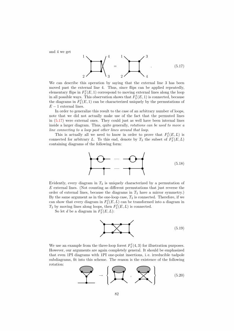
and 4 we get

2

1

3

4

=

2

1

4

3

. (5.17)

We can describe this operation by saying that the external line 3 has beenmoved past the external line 4. Thus, since flips can be applied repeatedly,elementary flips in F I

3 (E, 1) correspond to moving external lines along the loopin all possible ways. This observation shows that F I

3 (E, 1) is connected, becausethe diagrams in F I

3 (E, 1) can be characterized uniquely by the permutations ofE − 1 external lines.

In order to generalize this result to the case of an arbitrary number of loops,note that we did not actually make use of the fact that the permuted linesin (5.17) were external ones. They could just as well have been internal linesinside a larger diagram. Thus, quite generally, rotations can be used to move aline connecting to a loop past other lines around that loop.

This is actually all we need to know in order to prove that F I3 (E,L) is

connected for arbitrary L. To this end, denote by T3 the subset of F I3 (E,L)

containing diagrams of the following form:

(5.18)

Evidently, every diagram in T3 is uniquely characterized by a permutation ofE external lines. (Not counting as different permutations that just reverse theorder of external lines, because the diagrams in T3 have a mirror symmetry.)By the same argument as in the one-loop case, T3 is connected. Therefore, if wecan show that every diagram in F I

3 (E,L) can be transformed into a diagram inT3 by moving lines along loops, then F I

3 (E,L) is connected.So let d be a diagram in F I

3 (E,L):

(5.19)

We use an example from the three-loop forest F I3 (4, 3) for illustration purposes.

However, our arguments are again completely general. It should be emphasizedthat even 1PI diagrams with 1PI one-point insertions, i. e. irreducible tadpolesubdiagrams, fit into this scheme. The reason is the existence of the followingrotation:

→

,

(5.20)

82

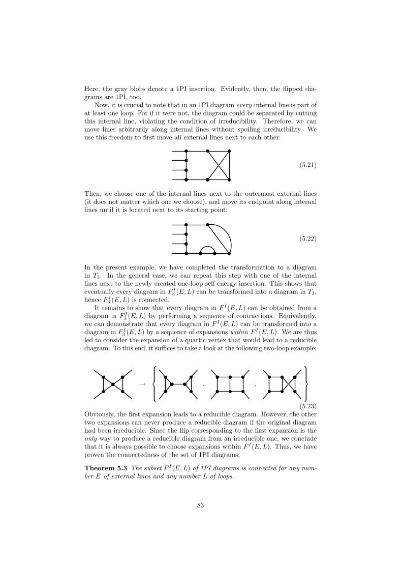
Here, the gray blobs denote a 1PI insertion. Evidently, then, the flipped dia-grams are 1PI, too.

Now, it is crucial to note that in an 1PI diagram every internal line is part ofat least one loop. For if it were not, the diagram could be separated by cuttingthis internal line, violating the condition of irreducibility. Therefore, we canmove lines arbitrarily along internal lines without spoiling irreducibility. Weuse this freedom to first move all external lines next to each other:

(5.21)

Then, we choose one of the internal lines next to the outermost external lines(it does not matter which one we choose), and move its endpoint along internallines until it is located next to its starting point:

(5.22)

In the present example, we have completed the transformation to a diagramin T3. In the general case, we can repeat this step with one of the internallines next to the newly created one-loop self energy insertion. This shows thateventually every diagram in F I

3 (E,L) can be transformed into a diagram in T3,hence F I

3 (E,L) is connected.It remains to show that every diagram in F I(E,L) can be obtained from a

diagram in F I3 (E,L) by performing a sequence of contractions. Equivalently,

we can demonstrate that every diagram in F I(E,L) can be transformed into adiagram in F I

3 (E,L) by a sequence of expansions within F I(E,L). We are thusled to consider the expansion of a quartic vertex that would lead to a reduciblediagram. To this end, it suffices to take a look at the following two-loop example:

→

, ,

(5.23)

Obviously, the first expansion leads to a reducible diagram. However, the othertwo expansions can never produce a reducible diagram if the original diagramhad been irreducible. Since the flip corresponding to the first expansion is theonly way to produce a reducible diagram from an irreducible one, we concludethat it is always possible to choose expansions within F I(E,L). Thus, we haveproven the connectedness of the set of 1PI diagrams:

Theorem 5.3 The subset F I(E,L) of 1PI diagrams is connected for any num-ber E of external lines and any number L of loops.

83

5.1.4 Amputated Diagrams

We turn now to the subset of amputated diagrams. We shall assume E ≥ 3 inthis section, because otherwise the notion of an amputated diagram does notmake sense.3 Amputated diagrams are in general reducible. However, ampu-tated diagrams are distinguished by the property that none of the two discon-nected pieces obtained by cutting through a single internal line is a diagramwith two external lines.

On the other hand, we do not exclude the possibility of one-point inser-tions. Therefore, we consider two subsets of amputated diagrams: the subsetsFA(E,L) and F ∗(E,L) of amputated diagrams with and without one-pointinsertions, respectively.

We shall first prove that the restrictions FA3 (E,L) and F ∗3 (E,L) to diagrams

without quartic vertices are connected. We begin with one-loop diagrams. Aone-loop diagram is always amputated if the loop contains three or more vertices.If the loop contains exactly two vertices, the diagram is amputated if none ofthe two tree subdiagrams obtained by removing the loop consist of a single line.Finally, if the loop contains just a single particle, corresponding to a one-looptadpole, the tree subdiagram obtained by removing the loop must have at leastfour external vertices.4

As an example, consider the following three diagrams from F3(4, 1), succes-sively linked by flips:

↔ ↔ ↔

(5.24)The latter three diagrams are amputated, while the former is not. This exampleagain demonstrates a kind of a graphical higher order operation representing anelementary rotation. In particular, observe that the displayed flips correspondto moving a line from the loop onto an adjecent line and vice versa. Combinedwith the operation of moving lines along loops, this means that sequences ofrotations are equivalent to all possible motions of lines along other lines withina diagram.

In the one-loop case, it is now easy to see that all diagrams in FA3 (E, 1)

are connected within FA3 (E, 1) to the set of irreducible diagrams F I

3 (E, 1): Wejust have to move all external lines onto the loop. This can only fail if in thebeginning the loop contains a single vertex, i. e. if the diagram contains a one-loop tadpole. In this case, for the original diagram to be amputated, it mustcontain the last diagram of (5.24) as subdiagram. But, reading the flips in (5.24)from right to left, we see that also in this case all intermediate diagrams areamputated. This proves the connectedness of FA

3 (E, 1). But F ∗3 (E, 1) is alsoconnected, because the flip to the one-loop tadpole is not required to connectthe other diagrams, whence one-point insertions can be omitted without spoiling

3In principle, amputation could be defined for one-point diagrams, i. e. E = 1. However,an amputated one-point diagram is an 1PI diagram, and 1PI diagrams have been treated inthe last section.

4We ignore here the one-loop self-energy diagrams, for which amputation is not actuallydefined. Anyway, these diagrams are 1PI, so they have been treated before.

84

the connectedness of the remaining diagrams.We would like to use a similar line of reasoning in the multi-loop case. To

this end, recall that connected diagrams, and hence amputated diagrams, havea skeleton expansion consisting of tree diagrams with 1PI functions for vertices,connected by full propagators. For our purposes, this means that an ampu-tated diagram consists of 1PI subdiagrams linked by single lines, as e. g. thefirst flipped diagram in (5.23). Now, every single line connecting two 1PI sub-diagrams defines a four-point subdiagram, the rotations of which will join thetwo 1PI subdiagrams into a single one:

→

,

(5.25)

Consequently, every diagram in FA3 (E,L) can be transformed by rotations

within FA3 (E,L) into an 1PI diagram in F I

3 (E,L). Since the latter set is con-nected, FA

3 (E,L) is connected, too. Again, the same applies if we omit one-pointinsertions, i. e. F ∗3 (E,L) is also connected.

We must now ask, whether all diagrams in FA(E,L) can be expanded withinFA(E,L) into diagrams in FA

3 (E,L), and similar for F ∗(E,L). Let us considerF ∗(E,L) first. By an argument similar to the one used in the last section, ifone expansion of a quartic vertex leads to a non-amputated diagram, there isalways another one that does not:5

→

,

(5.26)

Thus, F ∗(E,L) is connected.If one-point insertions are taken into account, these can be rotated away as

in (5.20), unless they are inserted into a quartic vertex. In this case, the quarticvertex has to be expanded first, but this may lead to a non-amputated diagramif external lines are coupled to the quartic vertex:

→

, ,

(5.27)

We have displayed the case of a one-loop tadpole, but clearly the argumentapplies to the general case as well. Now, if at least one of the three non-tadpolelines is not an external one, the insertion of the tadpole in this line is stillan amputated diagram. The tadpole can then again be transformed away asin (5.20), and all our previous arguments remain valid. Only if all non-tadpolelines at the quartic vertex are external lines is it impossible to avoid a non-amputated intermediate diagram. This case, which must be noted as a special

5Due to coinciding vertices, two expansions are identical here.

85

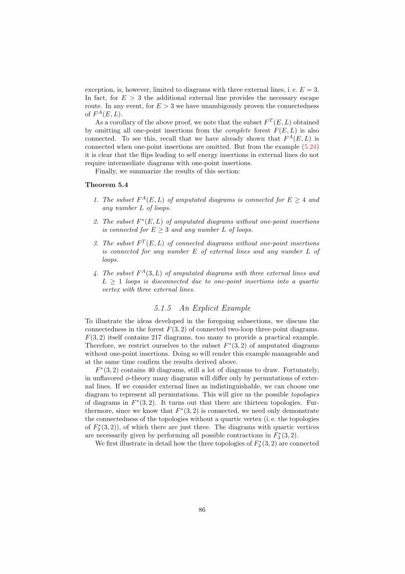
exception, is, however, limited to diagrams with three external lines, i. e. E = 3.In fact, for E > 3 the additional external line provides the necessary escaperoute. In any event, for E > 3 we have unambigously proven the connectednessof FA(E,L).

As a corollary of the above proof, we note that the subset FT (E,L) obtainedby omitting all one-point insertions from the complete forest F (E,L) is alsoconnected. To see this, recall that we have already shown that FA(E,L) isconnected when one-point insertions are omitted. But from the example (5.24)it is clear that the flips leading to self energy insertions in external lines do notrequire intermediate diagrams with one-point insertions.

Finally, we summarize the results of this section:

Theorem 5.4

1. The subset FA(E,L) of amputated diagrams is connected for E ≥ 4 andany number L of loops.

2. The subset F ∗(E,L) of amputated diagrams without one-point insertionsis connected for E ≥ 3 and any number L of loops.

3. The subset FT (E,L) of connected diagrams without one-point insertionsis connected for any number E of external lines and any number L ofloops.

4. The subset FA(3, L) of amputated diagrams with three external lines andL ≥ 1 loops is disconnected due to one-point insertions into a quarticvertex with three external lines.

5.1.5 An Explicit Example

To illustrate the ideas developed in the foregoing subsections, we discuss theconnectedness in the forest F (3, 2) of connected two-loop three-point diagrams.F (3, 2) itself contains 217 diagrams, too many to provide a practical example.Therefore, we restrict ourselves to the subset F ∗(3, 2) of amputated diagramswithout one-point insertions. Doing so will render this example manageable andat the same time confirm the results derived above.

F ∗(3, 2) contains 40 diagrams, still a lot of diagrams to draw. Fortunately,in unflavored φ-theory many diagrams will differ only by permutations of exter-nal lines. If we consider external lines as indistinguishable, we can choose onediagram to represent all permutations. This will give us the possible topologiesof diagrams in F ∗(3, 2). It turns out that there are thirteen topologies. Fur-thermore, since we know that F ∗(3, 2) is connected, we need only demonstratethe connectedness of the topologies without a quartic vertex (i. e. the topologiesof F ∗3 (3, 2)), of which there are just three. The diagrams with quartic verticesare necessarily given by performing all possible contractions in F ∗3 (3, 2).

We first illustrate in detail how the three topologies of F ∗3 (3, 2) are connected

86

by flips:

1

2 3

4 5 =

5

4

2 31 =

5

1 32 4

l

1

2 3

4 5 = 34

15

2=

5

1 3

2

4

l

1

2 3

5

4= 3

4 15

2

(5.28)

The diagrams are drawn in the left column in what could be called a conven-tional style. The middle and right column show how the flipped four-pointsubdiagrams—displayed in dashed line style—are embedded in these diagrams,leading to rather unconventional drawings. We denote the three topologies ofF ∗3 (3, 2) from top down as crossed ladder, ladder and self energy topology, re-spectively.

Note that the vertices are labeled in the above diagrams only only to easerecognition of the topologies. When comparing topologies, these labels have tobe forgotten. On the other hand, when we discuss the diagrams in F ∗3 (3, 2), thelabels 1, 2, and 3 must be kept to distinguish external lines.

Let us first count the number of diagrams in F ∗3 (3, 2): The permutations ofexternal lines (i. e. of the labels 1, 2, and 3) produce three different diagramsfor the ladder and self energy topology. On the other hand, every permutationof external lines leaves the crossed ladder invariant. Thus, F ∗3 (3, 2) consists ofseven diagrams, one crossed ladder, three ladders and three self energies.

Next we need the flips in F ∗3 (3, 2). We begin with the most symmetricdiagram, the crossed ladder, which we abbreviate as C. Due to the symmetryof C, every flip must lead to a ladder:

C =

1

2 3

→

1

2 3,

2 3

1

,

3

1

2

≡ L1, L2, L3

(5.29)

87

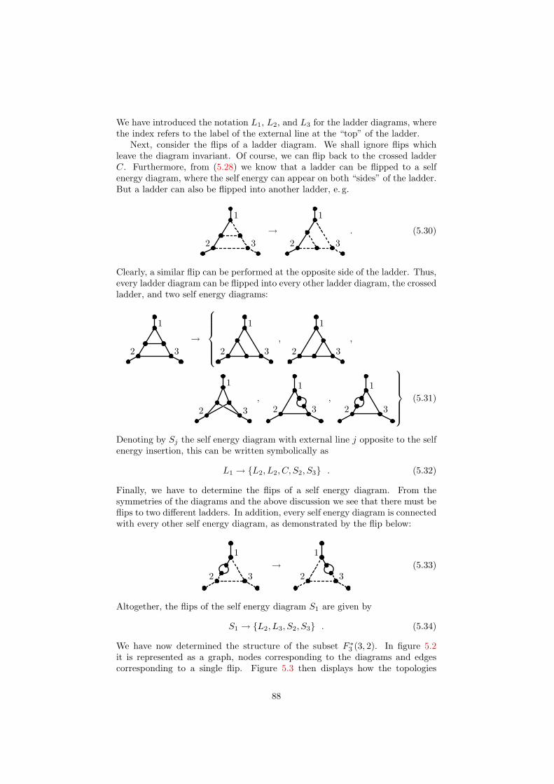
We have introduced the notation L1, L2, and L3 for the ladder diagrams, wherethe index refers to the label of the external line at the “top” of the ladder.

Next, consider the flips of a ladder diagram. We shall ignore flips whichleave the diagram invariant. Of course, we can flip back to the crossed ladderC. Furthermore, from (5.28) we know that a ladder can be flipped to a selfenergy diagram, where the self energy can appear on both “sides” of the ladder.But a ladder can also be flipped into another ladder, e. g.

1

2 3→

2 3

1

. (5.30)

Clearly, a similar flip can be performed at the opposite side of the ladder. Thus,every ladder diagram can be flipped into every other ladder diagram, the crossedladder, and two self energy diagrams:

1

2 3→

2 3

1

,

3

1

2,

1

2 3,

2 3

1,

3

1

2

(5.31)

Denoting by Sj the self energy diagram with external line j opposite to the selfenergy insertion, this can be written symbolically as

L1 → L2, L2, C, S2, S3 . (5.32)

Finally, we have to determine the flips of a self energy diagram. From thesymmetries of the diagrams and the above discussion we see that there must beflips to two different ladders. In addition, every self energy diagram is connectedwith every other self energy diagram, as demonstrated by the flip below:

3

1

2→

2 3

1(5.33)

Altogether, the flips of the self energy diagram S1 are given by

S1 → L2, L3, S2, S3 . (5.34)

We have now determined the structure of the subset F ∗3 (3, 2). In figure 5.2it is represented as a graph, nodes corresponding to the diagrams and edgescorresponding to a single flip. Figure 5.3 then displays how the topologies

88

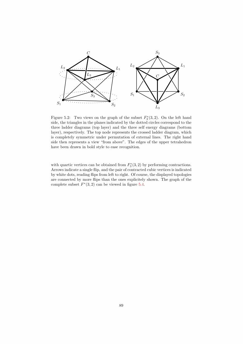
S2

S3

S1

L1L2

L3

C

L1L2

L3

S1 S2

S3

C

Figure 5.2: Two views on the graph of the subset F ∗3 (3, 2). On the left handside, the triangles in the planes indicated by the dotted circles correspond to thethree ladder diagrams (top layer) and the three self energy diagrams (bottomlayer), respectively. The top node represents the crossed ladder diagram, whichis completely symmetric under permutation of external lines. The right handside then represents a view “from above”. The edges of the upper tetrahedronhave been drawn in bold style to ease recognition.

with quartic vertices can be obtained from F ∗3 (3, 2) by performing contractions.Arrows indicate a single flip, and the pair of contracted cubic vertices is indicatedby white dots, reading flips from left to right. Of course, the displayed topologiesare connected by more flips than the ones explicitely shown. The graph of thecomplete subset F ∗(3, 2) can be viewed in figure 5.4.

89

→

→ →

→

→ →

→ →

→ →

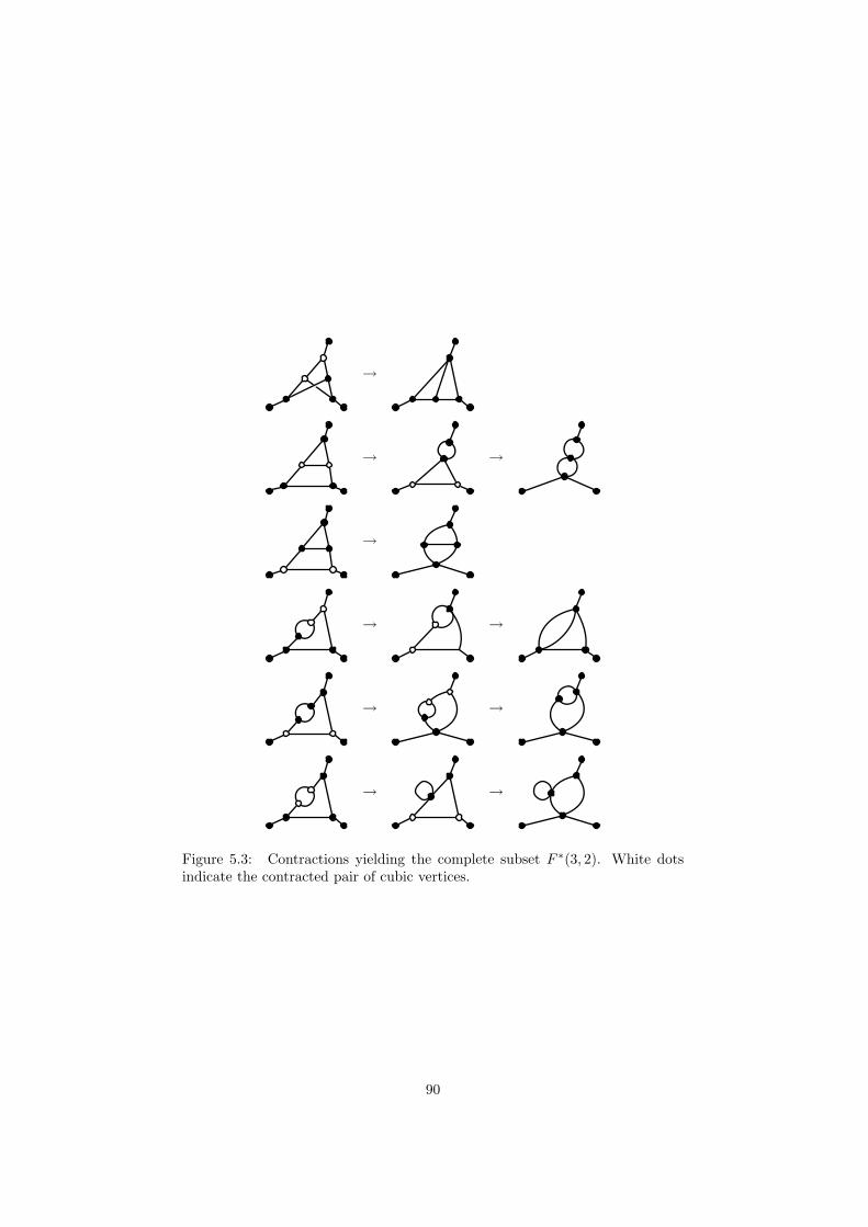
Figure 5.3: Contractions yielding the complete subset F ∗(3, 2). White dotsindicate the contracted pair of cubic vertices.

90

Figure 5.4: The graph of the complete subset F ∗(3, 2). Solid lines correspond torotations, dotted lines to contractions or expansions. In the center of the forest,we recognize the subset F ∗3 (3, 2). The view corresponds to the one displayed inthe right hand side of figure 5.2.

91

—6—Flips and Groves in Gauge Theories

In this chapter, we study the groves of connected Green’s functions in gaugetheories, employing the gauge flips, as defined in section 4.3. We shall arguethat the formalism of gauge flips and groves is mainly useful in spontaneouslybroken gauge theories. To this end, we briefly discuss the situation in QCD,as an example of an unbroken gauge theory. After that, we turn to our maingoal, the classification of groves of connected Green’s functions in the (minimal)Standard Model, the external lines of which correspond to physical particles.

It will then prove extremely useful to express the possible actions of gaugeflips in terms of more intuitive, higher level graphical transformations of Feyn-man diagrams, such as shifting a certain line along other lines of a diagram,breaking up a loop or joining two loops into a single one. These operations,called gauge motions will enable us to determine the structure of SM forests forvery general SM forests. We then turn to a specific example, which we discussin much detail. Finally, we compare the theoretical results thus obtained withthe results of an investigation by means of a computer program implementingthe decomposition of the forest by gauge flips as we have described it.

6.1 Flips in Gauge Theories

In the previous chapter we have investigated the forest F (E,L) of connectedFeynman diagrams in unflavored φ-theory. Flips were interpreted as higher levelgraphical operations on Feynman diagrams, through which the connectednessof the complete forest F (E,L) as well as various subsets could be proven. Whilethe connectedness of these subsets is of considerable practical interest, it hasno physical significance. In particular, amplitudes in unflavored φ-theory arenot constrained by any symmetries. Consequently, there are no relations amongFeynman diagrams induced by a gauge symmetry.

The situation is different in gauge theories. As we have demonstrated atlength in the first part of this work, the STIs in gauge theories induce relationsamong diagrams. In particular, in chapter 4 we proved that the groves of aconnected Green’s function G, i. e. the minimal gauge invariant subsets of G,can be constructed by applying gauge flips to diagrams of G.

Now, if we forget about the flavors pertaining to the lines of a diagram d in G,we can treat d as a diagram in unflavored φ-theory, because the renormalizableinteractions of a gauge theory are covered by the interaction degrees of φ-theory.The gauge flips in d are then just a subset of all possible flips of d. Consequently,

92

under gauge flips the forest F (G) of G will fall into disjoint subsets, which arejust the groves of G.

Since gauge flips have already been defined in 4.3—more specifically, in (4.53),(4.56), and (4.58)—we are now in principle in a position to analyze the struc-ture of the groves in a general gauge theory. However, it turns out that, inorder to obtain useful results, we have to be sufficiently explicit about the fieldcontent of the gauge theory. Therefore, we will discuss the QCD and the SM,as paradigms for an unbroken and broken gauge theory, respectively, in detail.The generalization of our results to other gauge theories should then be obvious.

6.2 Gauge Flips in QCD

Gauge flips develop their full power only in spontaneously broken gauge the-ories. To appreciate why this is the case, consider QCD as an example of anunbroken gauge theory. We have already mentioned in the introduction thatthe most efficient ways to calculate QCD amplitudes actually abandon the def-inition of the amplitude in terms of a sum of all possible Feynman diagrams.[1]Nevertheless, let us see what gauge flips have to say.

The elementary gauge flips of four-gluon subdiagrams are given by the trans-formations among the set of diagrams contributing to the four-gluon connectedGreen’s function at tree level: , , ,

(6.1)

Essentially, this set of diagrams is identical to the set F (4) of diagrams inunflavored φ-theory. This means that a pure gluon forest at tree level is nodifferent from the unflavored forest F (E). In particular, the forest of puregluon connected Green’s function at tree level always consists of a single grove.The same applies in higher orders, if we consider QCD without quarks, becausethe diagrams with ghost loops cannot produce separate groves. Thus, in anunbroken pure Yang-Mills theory, the forest can never be partitioned in morethan a single grove.

If quarks are taken into account, the situation changes because then diagramswith a fixed number of quark loops are gauge invariant by themselves. Thiscan be demonstrated using gauge flips, because a gauge flip never changes thenumber of fermion loops, as is apparent from the set of four-point diagrams witha single quark line, defining the relevant elementary gauge flips: , ,

(6.2)

Thus, the formalism of gauge flip confirms the known fact [25] that the STIsin gauge theories apply separately to diagrams with a fixed number of fermionloops.

93

However, gauge flips were invented in order to search for a finer partitioningthan the partitioning according to the number of fermion loops. On the otherhand, as we have argued above, the usual treatment of QCD diagrams impliesthat, concerning flips, they behave effectively like unflavored diagrams. In otherwords, the group structure of QCD is completely ignored by the QCD gaugeflips in (6.1) and (6.2).

To illustrate this, we consider the four-quark connected Green’s functionat one-loop level. Assuming, for simplicity, that the flavors of the quarks aredifferent, the diagrams without a quark loop form a single grove:

, , , ,

, , , ,

, . . .

(6.3)

We have omitted all but one of the four diagrams with a quark self energy inan external leg.

Without any specific information on the colors of gluon and quarks, wecannot exclude a single diagram of this set. On the other hand, the structureconstants fabc of the color gauge group SU(3) do vanish for many choices ofcolor indices. For instance, in the usual Gell-Man basis, the structure constantsfabc are identically zero if both a and b are equal to 3 or 8, because the Gell-Manmatrices λ3 and λ8 mutually commute. Thus, if we choose the two gluons in thelast two diagrams of (6.3) to correspond to these generators, the diagrams withthe triple gluon vertex will be absent. This, in turn, implies that the followingsubsets of the above grove are in fact groves themselves:

ab

c1

c1

c2

c2

, a

b

c1

c1

c2

c2

,

ab

c1

c1

c2

c2

(6.4)

94

b

a

c1

c1

c2

c2

, a

b

c1

c1

c2

c2

,

ab

c1

c1

c2

c2

(6.5)

b

a

c1

c1

c2

c2

,

a

bc1

c1

c2

c2

(6.6)

Here, the color indices a and b of the gluons take on the values 3 or 8. Ofcourse, these diagrams are identically zero if either of a or b is 3 and one ofthe quark colors c1 or c2 has the value “blue”, because λ3 yield zero on the“blue” component of the quark color multiplet. Note, however, that for othercombinations of gluon colors, like 1 and 2, 4 and 5, or 6 and 7, the diagramsin (6.3) will all be present and form a single grove.

The origin of this additional structure in the QCD forests is caused by theintroduction of an arbitrary but fixed basis in color space. This was done hereby choosing the representation of Gell-Man for the generators of SU(3). Asa matter of principle, there is nothing wrong with such an approach. On theother hand, Green’s functions with colored external states are unphysical dueto confinement in QCD. Therefore, in all practical applications, color sums willhave to be performed. It is then much more convenient not to use an explicitbasis, because, at least if amplitudes are defined through Feynman diagrams,the color structure can always be separated from the Lorentz and kinematicalstructure. Color sums can then be performed by group theory techniques, whichis generally more efficient than using the brute force method of summing overa fixed basis. But without specifying an explicit color value for the two inter-mediate gluons, the forest has no structure but the one induced by the numberof fermion loops. Thus, the real reason why gauge flips are not very useful forQCD is that in QCD the gauge symmetry is unbroken, such that every choiceof basis in color space is necessarily an arbitrary one.

To turn the argument on its head, this means that gauge flips will be usefulif physics chooses a direction in the representation space of the gauge group.This happens precisely in gauge theories with spontaneous symmetry breaking,where the choice of ground state fixes a direction in group space, at least forthe broken generators of the gauge group. We will discuss this in detail in thenext section.

6.3 Gauge Flips and Groves in the Standard Model

To determine the structure of Standard Model (SM) forests, we must list thepossible gauge flips in some detail, taking into account the real field content ofthe SM. In order not to get lost in notation, we use a collective notation for theSM fields where this is appropriate. For instance, we shall distinguish quarksand leptons only if QCD couplings are considered. Also, we shall use a singlesymbol for the photon as well as the Z0 boson (together with its associated

95

Goldstone boson). To be specific, the following notation is employed for thefields of the SM:1

W±µ , φ

± → (6.7a)

Aµ, Z0µ, φ

0 → (6.7b)

H → (6.7c)

`, ν`, q → (6.7d)

Gaµ → (6.7e)

Ghosts can be ignored for the determination of groves.It is important to note here, that we consider only fermions in the dublet

representation of SU(2), that is, the usual quarks and leptons. If other rep-resentations are of interest, as e. g. in supersymmetric extensions of the SM,the set of gauge flips involving fermions, discussed in the next section, andhence the structure of the forest, will change. We will indicate the places wheremodifications would be necessary.

Also, we consider fermions generically as massive. This means that fermionsgenerally are coupled to the H boson and the Goldstone bosons. Later, we shallinvestigate the changes brought about by considering fermions as massless indetail. We shall, however, indicate briefly the places where a vanishing fermionmass would make a difference.

Sometimes, we have to distinguish clearly between photon and Z0. In thiscase, the latter shall be represented by a zigzag line:

Z0µ, φ

0 → (6.8)

Note that we shall refer to the bosons of the electroweak (EW) sector of theSM, i. e. H, Aµ, Z0

µ, Wµ, and the associated Goldstone bosons, collectively asEW bosons, or even just as bosons, if no confusion is possible. Gluons, on theother hand, shall always be referred to as such.

6.3.1 Gauge Flips

Neglecting the flips of ghost subdiagrams in (4.58), the gauge flips in the SMare given by the transformations among the four-point subdiagrams with atleast one external gauge boson as well as the five-point subdiagrams with atleast one external gauge boson and three H bosons. The SM gauge flips havebeen derived in the context of tree level diagrams in [5]. We list them here forreference purposes. On one hand, there are the four-point subdiagrams withonly bosonic external lines: , , ,

(6.9a)

1We denote the field corresponding to the photon as Aµ. However, we shall refer to thephoton as a particle as γ.

96

, ,

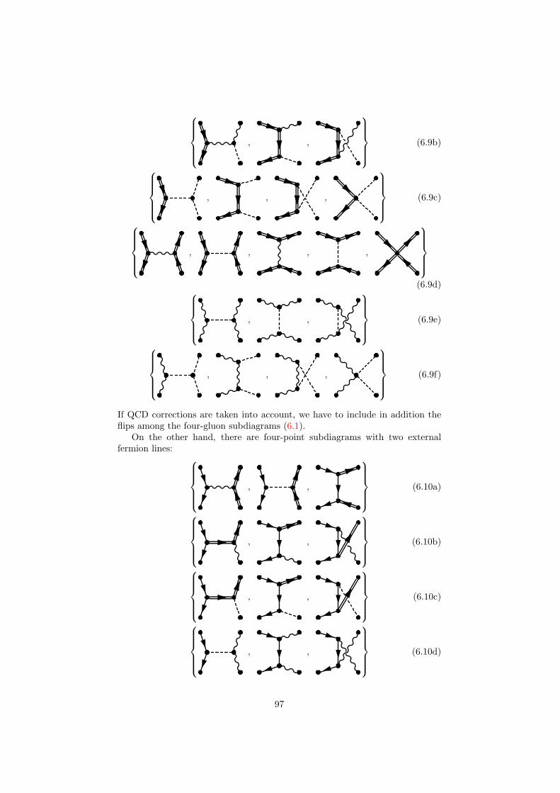
(6.9b)

, , ,

(6.9c)

, , , ,

(6.9d) , ,

(6.9e)

, , ,

(6.9f)

If QCD corrections are taken into account, we have to include in addition theflips among the four-gluon subdiagrams (6.1).

On the other hand, there are four-point subdiagrams with two externalfermion lines: , ,

(6.10a)

, ,

(6.10b)

, ,

(6.10c)

, ,

(6.10d)

97

, ,

(6.10e)

,

(6.10f)

,

(6.10g)

Note that, in the last subset, we have chosen a plain line to represent any neutralEW boson. Here, we have to add the quark-gluon subdiagrams from (6.2) toaccount for QCD corrections.

This set of gauge flips is the correct one for massive fermions in the dubletrepresentation of SU(2). For massless fermions, the subdiagrams with couplingsof the H boson to the fermion line are absent. We do not consider fermions inrepresentations of SU(2) other than the dublet representation in this work.However, we would like to mention that, for fermions in other representationsof SU(2), additional gauge flips appear of four-point subdiagrams with twoW bosons of like charge. Such diagrams simply cannot exist for fermions in thedublet representation.2

Finally, there are the following gauge flips of five-point subdiagrams: , , ,

(6.11)

, , ,

(6.12)

Using a collective notation for SM fields comes at the price that we are notguaranteed the existence of the displayed subdiagrams for all allowed choicesof external lines. For instance, neutrinos will not couple to the photon. Moreimportantly, for massless fermions no coupling to the H boson exists. Masslessfermions will be discussed in detail later. However, we note that in the SM everyfermion couples to the Z0 boson, which is a simple consequence of the SU(2)part in the SM gauge group SU(2)×U(1). This fact will be put to use later inthe determination of the groves of SM connected Green’s functions.

2For a discussion of the structure of the forest in and SU(2) gauge theory with fermionsin arbitrary irreducible representations of SU(2), see [6].

98

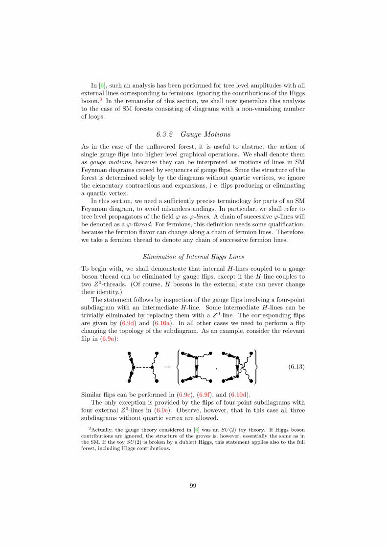
In [6], such an analysis has been performed for tree level amplitudes with allexternal lines corresponding to fermions, ignoring the contributions of the Higgsboson.3 In the remainder of this section, we shall now generalize this analysisto the case of SM forests consisting of diagrams with a non-vanishing numberof loops.

6.3.2 Gauge Motions

As in the case of the unflavored forest, it is useful to abstract the action ofsingle gauge flips into higher level graphical operations. We shall denote themas gauge motions, because they can be interpreted as motions of lines in SMFeynman diagrams caused by sequences of gauge flips. Since the structure of theforest is determined solely by the diagrams without quartic vertices, we ignorethe elementary contractions and expansions, i. e. flips producing or eliminatinga quartic vertex.

In this section, we need a sufficiently precise terminology for parts of an SMFeynman diagram, to avoid misunderstandings. In particular, we shall refer totree level propagators of the field ϕ as ϕ-lines. A chain of successive ϕ-lines willbe denoted as a ϕ-thread. For fermions, this definition needs some qualification,because the fermion flavor can change along a chain of fermion lines. Therefore,we take a fermion thread to denote any chain of successive fermion lines.

Elimination of Internal Higgs Lines

To begin with, we shall demonstrate that internal H-lines coupled to a gaugeboson thread can be eliminated by gauge flips, except if the H-line couples totwo Z0-threads. (Of course, H bosons in the external state can never changetheir identity.)

The statement follows by inspection of the gauge flips involving a four-pointsubdiagram with an intermediate H-line. Some intermediate H-lines can betrivially eliminated by replacing them with a Z0-line. The corresponding flipsare given by (6.9d) and (6.10a). In all other cases we need to perform a flipchanging the topology of the subdiagram. As an example, consider the relevantflip in (6.9a):

→

,

(6.13)

Similar flips can be performed in (6.9c), (6.9f), and (6.10d).The only exception is provided by the flips of four-point subdiagrams with

four external Z0-lines in (6.9e). Observe, however, that in this case all threesubdiagrams without quartic vertex are allowed.

3Actually, the gauge theory considered in [6] was an SU(2) toy theory. If Higgs bosoncontributions are ignored, the structure of the groves is, however, essentially the same as inthe SM. If the toy SU(2) is broken by a dublett Higgs, this statement applies also to the fullforest, including Higgs contributions.

99

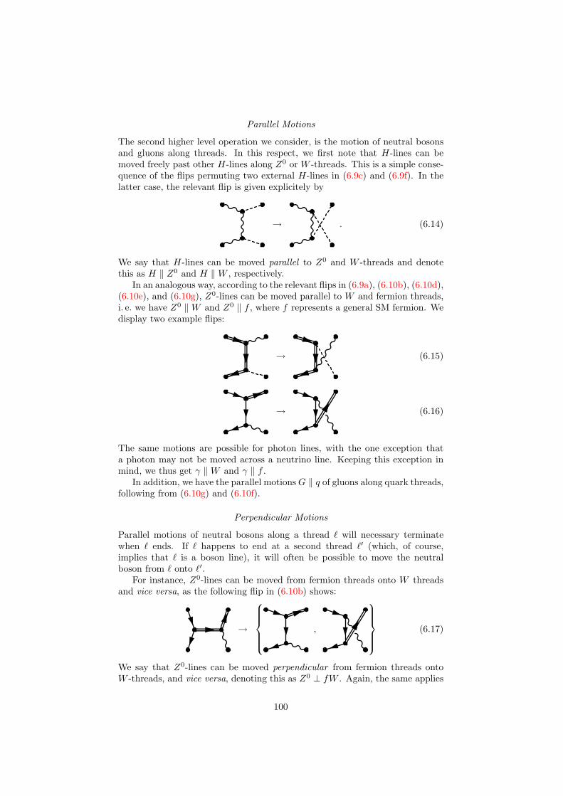
Parallel Motions

The second higher level operation we consider, is the motion of neutral bosonsand gluons along threads. In this respect, we first note that H-lines can bemoved freely past other H-lines along Z0 or W -threads. This is a simple conse-quence of the flips permuting two external H-lines in (6.9c) and (6.9f). In thelatter case, the relevant flip is given explicitely by

→ . (6.14)

We say that H-lines can be moved parallel to Z0 and W -threads and denotethis as H ‖ Z0 and H ‖W , respectively.

In an analogous way, according to the relevant flips in (6.9a), (6.10b), (6.10d),(6.10e), and (6.10g), Z0-lines can be moved parallel to W and fermion threads,i. e. we have Z0 ‖W and Z0 ‖ f , where f represents a general SM fermion. Wedisplay two example flips:

→ (6.15)

→ (6.16)

The same motions are possible for photon lines, with the one exception thata photon may not be moved across a neutrino line. Keeping this exception inmind, we thus get γ ‖W and γ ‖ f .

In addition, we have the parallel motionsG ‖ q of gluons along quark threads,following from (6.10g) and (6.10f).

Perpendicular Motions

Parallel motions of neutral bosons along a thread ` will necessary terminatewhen ` ends. If ` happens to end at a second thread `′ (which, of course,implies that ` is a boson line), it will often be possible to move the neutralboson from ` onto `′.

For instance, Z0-lines can be moved from fermion threads onto W threadsand vice versa, as the following flip in (6.10b) shows:

→

,

(6.17)

We say that Z0-lines can be moved perpendicular from fermion threads ontoW -threads, and vice versa, denoting this as Z0 ⊥ fW . Again, the same applies

100

for photon lines, i. e. there is a perpendicular motion γ ⊥ fW . Note that thereis no restriction for photon lines if the photon is moved from the fermion threadonto the W -thread. For if the last line of the fermion thread was a neutrinoline, the photon would not have been there in the first place.

For H-lines, there are three perpendicular motions. Instead of displaying therelevant flips explicitely, we will refer to the respective subsets. Thus, (6.10c)implies H ⊥ fW , (6.10e) implies H ⊥ fZ0, and (6.9b) implies H ⊥ Z0W .

Observe that we have chosen to define the perpendicular motions of H-linesinvolving fermions as motions from the fermion thread onto the gauge bosonthread. The reverse motions, from a gauge boson thread onto a fermion thread,are possible only for a massive fermion thread. As we shall later see, the lackof this gauge motion for massless fermions leads to additional structure of theSM forests with massless fermions.

Finally, for gluons we have the perpendicular motion G ⊥ qG, which followsfrom (6.2). Note that the interpretation is slightly different in this case. Inparticular, it does not actully make sense to speak of a gluon thread, becausecolor can flow into all three directions at a triple gluon vertex. However, it iscertainly true that a gluon coupled to quark thread can always be moved ontoa neighboring gluon line. We shall understand G ⊥ qG in this way.

Crossover Motions

There are yet more intricate motions of neutral bosons. In particular, while aZ0-line certainly cannot move parallel to a Z0-thread, it can use a Z0-line toswitch from a W -thread to another W -thread or a fermion thread. For the caseof two W -threads, the relevant flips come from (6.9d) and (6.9a):

→ → →

(6.18)We say that the Z0-line is moved crossover from W -thread to W -thread, usinga Z0-line as a bridge, and denote this as Z0 ×WZ0W .

For the case of one fermion thread and one W -thread we need (6.10a) andthe perpendicular motion Z0 ⊥ fW :

→ → →

(6.19)Thus, we have Z0×fZ0W . Again, for photons the identical motions γ×WZ0Wand Z0 × fZ0W are possible.

Finally, using (6.9f), we can show that H has the crossover motion H ×Z0HZ0. That is, a H-line can use another H-line as a bridge from Z0-thread

101

to Z0-thread:

→ → →

(6.20)Note that H × WZ0W and H × fZ0W as well as H × fZ0f , Z0 × fWf ,and G × qGq, although valid motions with the effect of a crossover motion,are actually sequences of perpendicular motions. In contrast, the real crossovermotions displayed above cannot be represented as sequences of perpendicularmotions only.

Crossing Threads

The last two operations we shall need in order to discuss the structure of SMforests are concerned with the crossing of threads. Actually, we have seen suchan operation at work in the discussion of crossover motions. To see this, take alook back at (6.18). In the first diagram, we recognize twoW -threads, connectedby a Z0-line. The flip to the second diagram then breaks up both W -threadsand reconnects them in a different way. In particular, if we take the arrows toindicate a direction along the threads, the tail of the first thread is joined ontothe head of the second thread, and vice versa. We say that the two W -threadshave been crossed.

To appreciate the significance of thread crossing, suppose the diagramsin (6.18) were contributions to the amplitude (or, rather, connected Green’sfunction) for the processW+W− →W+W−Z0. In that case, beginning and endof the W threads are distinguished by the momenta of the external W bosons.Thread crossing then realizes the two possible ways of connecting the externalW -lines into threads. As we shall see below, this generalizes to the case of morethan two W -threads.

Thread crossing is also possible for two Z0-threads connected by an H-line,which follows readily from (6.9e). In fact, since a Z0-thread has no intrinsicdirection, the broken up threads can be reconnected in all possible ways.

Absorbing Closed Threads

Thread crossing can be used to absorb a closed W -thread or Z0-thread, i. e. aW -loop or Z0-loop, into another W -thread or Z0-thread, respectively. We listthis case separately, because it is very important for the structure of the SMforests.

As an example, consider the case of a closed W -thread:

→ (6.21)

102

In an analogous way, closed Z0-threads can be absorbed into into Z0-threads.Note that the absorbing thread can be either an open thread or a closed thread.

The possibility of absorbing closed threads clearly shows that the number ofW -loops and Z0-loops is not invariant under gauge flips. Of course, the totalnumber of loops remains fixed.

Elimination of H4 Vertices

This gauge motion answers the question under which conditions a H4 vertexcan be expanded by a gauge flip. This is important, because the expansion of aH4 vertex as a four-point subdiagram into a subdiagram with two H3 vertices isnot a gauge flip. Consequently, diagrams with different numbers of H4 verticeswould be candidates for separate invariant subsets, unless the five-point gaugeflips can be used to perform this transformation indirectly.

This is, however, the case, as is apparent from (6.11) and (6.12). For def-initeness, we consider the former five-point subdiagrams with two W bosons.We first use a five-point flip to replace the H4 vertex by a W+W−H2 vertex:

→ (6.22)

The W+W−H2 vertex can then be expanded by a gauge flip of a four-pointsubdiagram:

→ (6.23)

In the same way, the H4 vertex can be expanded if the W -thread is replaced bya Z0-thread. Thus, if a H4 vertex is coupled to a W -thread or Z0-thread, thethree H-lines not connected to the thread can be absorbed onto the thread bya gauge motion.

Summary of Gauge Motions

Let us summarize the set of valid gauge motions, i. e. the possible transforma-tions of Feynman diagrams achievable by sequences of gauge flips:

1. Elimination of internal H-lines, except for H-lines connecting two Z0-threads.

2. The parallel motions H ‖ Z0, H ‖ W , Z0 ‖ W , Z0 ‖ f , γ ‖ W ,γ ‖ f 6= ν, G ‖ q.

3. The perpendicular motions Z0 ⊥ fW , γ ⊥ fW , H ⊥ fW , H ⊥ fZ0,H ⊥ Z0W , G ⊥ qG.

4. The crossover motions Z0×WZ0W , Z0×fZ0W , γ×WZ0W , γ×fZ0W ,H × Z0HZ0.

103

5. Thread crossing of two W -threads or two Z0-threads.

6. Absorption of closed W -threads and Z0-threads.

7. Elimination of H4 vertices coupled to W -threads or Z0-threads.

6.3.3 Pure Boson Forests

In this section, we shall analyze the structure of SM forests without fermions.Connected Green’s functions without any fermionic contributions are of lim-ited direct physical interest, because the initial and final states of high energyscattering processes usually contain many fermions. However, knowledge of thestructure of the pure boson forests will prove indispensable for unraveling thestructure of general forests.

Pure gluon forests have been discussed in 6.2. On the other hand, a pureboson forest involving EW bosons can never contain gluons, because color SU(3)commutes with SU(2) × U(1), and hence gluons do not couple to EW bosons.Thus, we can ignore gluons in this section.

In the following, we leave the number L of loops of the diagrams in the forestsimplicit. A general SM forest is then characterized completely by the externalstate E , i. e. the number and nature of the external lines. Given a particularexternal state E , we shall denote the corresponding forest as F (E). Note thatwe characterize all external lines by particle labels corresponding to outgoingparticles. In the SM, this implies that the sum over the electromagnetic chargesof the external particles vanishes.

We shall distinguish pure boson forests according to the number NW ofexternal W lines. Owing to charge conservation, this number must be a multipleof two. As we are going to demonstrate shortly, the number of neutral externalboson lines is irrelevant for the determination of the structure of the forest.Therefore, we denote a purely bosonic external state with NW external W -linesas B(NW ).

Diagrams With a Single Open W -Thread

We begin our discussion with the forest F (B(2)) corresponding to external statescontaining exactly one W+ and one W− boson, and in addition an arbitrarynumber of neutral bosons. Because all interactions in the SM conserve the elec-tromagnetic charge, diagrams in F (B(2)) contain precisely one open W -thread,starting and terminating at two external vertices. We will now demonstratethat this W -thread is sufficient to make F (B(2)) connected under gauge flips.That is, F (B(2)) always consists of a single grove.

To prove this, we adopt a strategy similar to the one we used when we provedthe connectedness of subsets of the forest in unflavored φ-theory. In particular,we first restrict our attention to the subset F3(B(2)) of diagrams without aquartic vertex. Next, we shall designate a subset T3 of F3(B(2)), connectedunder gauge flips, with a canonical topology. Connectedness of F3(B(2)) thenfollows if we can show that every diagram in F3(B(2)) can be transformed intoa diagram in T3 by means of gauge motions.

To be specific, we choose the diagrams in T3 to have the following topology:

104

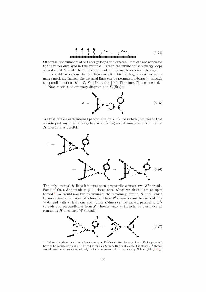
(6.24)

Of course, the numbers of self-energy loops and external lines are not restrictedto the values displayed in this example. Rather, the number of self-energy loopsshould equal L, while the numbers of neutral external bosons are arbitrary.

It should be obvious that all diagrams with this topology are connected bygauge motions. Indeed, the external lines can be permuted arbitrarily throughthe parallel motions H ‖W , Z0 ‖W , and γ ‖W . Therefore, T3 is connected.

Now consider an arbitrary diagram d in F3(B(2)):

d = (6.25)

We first replace each internal photon line by a Z0-line (which just means thatwe interpret any internal wavy line as a Z0-line) and eliminate as much internalH-lines in d as possible:

d →

→ → (6.26)

The only internal H-lines left must then necessarily connect two Z0-threads.Some of these Z0-threads may be closed ones, which we absorb into an openthread.4 We would now like to eliminate the remaining internal H-lines, whichby now interconnect open Z0-threads. These Z0-threads must be coupled to aW -thread with at least one end. Since H-lines can be moved parallel to Z0-threads and perpendicular from Z0-threads onto W -threads, we can move allremaining H-lines onto W -threads:

→ (6.27)

4Note that there must be at least one open Z0-thread, for else any closed Z0-loops wouldhave to be connected to the W -thread through a H-line. But in this case, the closed Z0-threadwould have been broken up already in the elimination of the connecting H-line. (Cf. (6.13))

105

The H-lines can now be eliminated again using the gauge flip (6.13). At thispoint, d has been transformed, using gauge motions, into a diagram d′ withoutinternal H-lines:

d′ → (6.28)

d′ must then necessarily consist of one open and an unspecified number of closedW -threads, interconnected by Z0-lines. That is, there can be no Z0-threadconsisting of more than a single Z0-line. But then all closed W -threads can beabsorbed into the single open W -thread by means of thread crossing:

d′ → (6.29)

The resulting diagram is easily transformed into a diagram of the form (6.24) byparallel motions along the W -thread. Therefore, F3(B(2)) is connected undergauge flips.

For this to imply that the complete forest F (B(2)), including diagrams withquartic vertices, is connected under gauge flips, we yet have to demonstratethat every diagram in F (B(2)) can be transformed into a diagram in F3(B(2))using gauge flips. This is readily seen to be true for diagrams without a H4

vertex, because all other quartic vertices involve gauge bosons, and hence theirexpansion is always a gauge flip. Thus, the only potential obstacle is providedby diagrams with H4 vertices. However, according to the gauge motion 7, thesecan be absorbed into the W -thread, thereby replacing the H4 vertex by twocubic vertices. This means that every diagram in F (B(2)) can be transformedinto a diagram in F3(B(2)) using gauge motions, as was to be shown.

Diagrams With Several Open W -Threads

We now consider the forests F (B(NW )) for NW > 2, which means that there areseveral open W -threads present. We claim that these forests are also connectedunder gauge flips.

The treatment of this case is very similar to the case of a single open W -thread. Indeed, given a diagram in F3(B(NW )), we can eliminate all internalH-lines and closed Z0-threads exactly as before. We then have a diagram withNW /2 open W -threads and any number of closed W -threads, interconnectedby Z0-lines. The closed W -threads are absorbed into open ones, no matterwhich. This leaves us with a diagram consisting of just NW /2 W -threads,

106

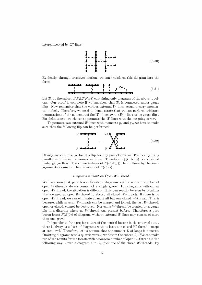
interconnected by Z0-lines:

(6.30)

Evidently, through crossover motions we can transform this diagram into theform:

(6.31)

Let T3 be the subset of F3(B(NW )) containing only diagrams of the above topol-ogy. Our proof is complete if we can show that T3 is connected under gaugeflips. Now remember that the various external W -lines actually carry momen-tum labels. Therefore, we need to demonstrate that we can perform arbitrarypermutations of the momenta of theW+-lines or the W−-lines using gauge flips.For definiteness, we choose to permute the W -lines with the outgoing arrow.

To permute two external W -lines with momenta p1 and p2, we have to makesure that the following flip can be performed:

p2

p1

→

p2

p1

(6.32)

Clearly, we can arrange for this flip for any pair of external W -lines by usingparallel motions and crossover motions. Therefore, F3(B(NW )) is connectedunder gauge flips. The connectedness of F (B(NW )) then follows by the samearguments as used in the discussion of F (B(2)).

Diagrams without an Open W -Thread

We have seen that pure boson forests of diagrams with a nonzero number ofopen W -threads always consist of a single grove. For diagrams without anopen W -thread, the situation is different. This can readily be seen by recallingthat we used an open W -thread to absorb all closed W -threads. If there is noopen W -thread, we can eliminate at most all but one closed W -thread. This isbecause, while several W -threads can be merged and joined, the last W -thread,open or closed, cannot be destroyed. Nor can a W -thread be created by a gaugeflip in a diagram where no W -thread was present before. Therefore, a pureboson forest F (B(0)) of diagrams without external W lines may consist of morethan one grove.

Independent of the precise nature of the neutral bosons in the external state,there is always a subset of diagrams with at least one closed W -thread, exceptat tree level. Therefore, let us assume that the number L of loops is nonzero.Omitting diagrams with a quartic vertex, we obtain the subset C3. We can makeuse of the results for the forests with a nonzero number of open W -threads in thefollowing way. Given a diagram d in C3, pick one of the closed W -threads. By

107

cutting aW -line, we obtain a diagram d′ with a single openW -thread. But theseare connected. Therefore, C3 is connected, too. As before the connectednessof all diagrams in F (B(0)) with at least one W -thread (including those withquartic vertices), follows from this result.

Next, consider the case where the external state contains a nonzero (even)number NZ of Z0 bosons. The subset of F (B(0)) of diagrams without anyW -thread then consists of diagrams with NZ/2 open and an arbitrary numberof closed Z0-threads. Denote by N3 the restriction of this subset to diagramswithout quartic vertices. Note that diagrams in N3 cannot contain a photonline, because photons do not couple to neutral bosons. On the other hand, N3

is non-empty even at tree level. We claim that N3 is connected under gaugeflips. To see this, choose an arbitrary diagram d in N3. We first eliminate asmany internal H-lines as possible. Afterwards, we absorb all closed Z0-threadsinto an open Z0-thread. This leaves us with a diagram d′ consisting of openZ0-threads, interconnected by H-lines:

(6.33)

Since H-lines can be moved parallel along Z0-threads and crossover from oneZ0-thread onto another, all diagrams inN3 can be transformed into the followingtopology:

(6.34)

By an argument similar to the one given below (6.31), arbitrary permutationsof external Z0-lines can be performed by crossing Z0-threads. Therefore, dia-grams of the form (6.34) are connected, hence N3 is connected, which in turnimplies that, for nonzero NZ, all diagrams in F3(B(0)) without a W -thread areconnected. Again, this implies that the subset of diagrams without a W -threadof the complete forest F (B(0)) is connected, because all quartic vertices can bereplaced by two cubic vertices through gauge motions, where H4 vertices areabsorbed into some Z0-thread.

This leaves us with an external state consisting of H bosons only. Thesubset of diagrams with at least one (closed) W -thread is connected by thesame arguments as before. Next, consider the subset of diagrams without W -thread, but with at least one (closed) Z0-thread (which, of course, requires anonzero number of loops). By arguments similar to the case of diagrams withone or more closed W -threads, this subset is connected under gauge flips. Theremaining diagrams contain neither a W -thread nor a Z0-thread, which, in thepresent context of pure boson forest, means that they contain H bosons only.Every such diagram is trivially gauge invariant, because it does not depend onunphysical degrees of freedom in any way.

108

Summary of the Structure of Pure Boson Forests

We collect the results about the pure boson forests F (B(NW )) with NW openW -threads in a theorem. To make our notation more concise, we shall refer toa diagram with at least one W -thread as a charged diagram, and to a diagramwithout a W -thread as a neutral diagram. Correspondingly, the terms chargedgrove and neutral grove are used to denote a grove containing only charged andonly neutral diagrams, respectively.5 The theorem about the pure boson forestcan then be stated as follows:

Theorem 6.1

1. A pure boson forest with external W bosons consists of a single grove.

2. A pure boson forest with external photons consists of a single grove.

3. A pure boson forest with an external state consisting solely of neutralbosons, at least one of which is a Z0 boson, decomposes into

(a) a grove containing all charged diagrams;

(b) a grove containing all neutral diagrams.

4. A pure boson forest with an external state consisting solely of H bosonsdecomposes into


(b) a grove containing all neutral diagrams with at least a single Z0-loop;

(c) a separate grove for each diagram without gauge boson lines.

6.3.4 General SM Forests

In this section, we investigate the structure of SM forests with massive fermions.Massless fermions will be discussed later on an explicit example.

As mentioned before, the STIs in gauge theories apply separately to diagramswith a fixed number of fermion loops.[25] In the present context, this can easilybe seen by inspection of the gauge flips involving fermion lines, (6.10) and (6.2).Indeed, none of these flips can create or destroy a fermion loop. It is then clearthat the groves of a general SM forest respect this structure. This can also beseen from the fact that, in principle, arbitrarily many fermion dublets can beadded to the SM Lagrangian without violating gauge invariance. Therefore, ifwe increase the number of fermion loops by one, can always imagine that theadditional fermion loop belongs to a new, distinct flavor. Consequently, thediagrams with an additional fermion loop must be separately gauge invariant.

Let us denote by F (E , λ) the subset of a general SM forest with externalstate E and λ fermion loops. We will refer to F (E , λ) as a subforest. The totalnumber L of loops is left implicit. (Of course, λ ≤ L.) More specifically, wedenote by E(Nf ) an external state containing Nf fermion lines, where, owingto fermion number conservation, Nf must be a multiple of two.

Like for the pure boson forest discussed in the last section, a subset S ofF (E , λ) is connected under gauge flips if and only if the subset S3 of diagrams

5This terminology for groves is justified, because, as we shall see, a grove can never containboth charged and neutral diagrams.

109

in S without a quartic vertex is connected. Therefore, we shall infer the decom-position of F (E , λ) from the subset of diagrams without a quartic vertex. Tokeep our notation compact, we shall not, however, introduce an extra notationfor this subset. It should then be implicitely understood that only diagramswithout a quartic vertex are to be considered.

In order to put the results of the last section to use in the investigation ofSM forests with fermions, we shall proceed according to the following generalstrategy. We will try to move as many boson lines as possible perpendicularfrom the fermion threads onto boson threads. Clearly, if all boson lines excepta single one can be stripped off the fermion lines, the remaining gauge motionsare just those of pure boson forests, for which the above results can be applied.

Note that, since diagrams without gauge bosons (including Goldstone bosons)are trivially gauge invariant, every such diagram forms a separate grove. Wewill mention these trivial groves briefly when they can occur. Our main focus is,however, on diagrams with at least one gauge boson line, where the cancellationof unphysical degrees of freedom is essential to ensure the consistency of thetheory.

Diagrams With a Single Open Fermion Thread

We begin by analyzing F (E(2), 0), i. e. the subforest of diagrams with a singleopen fermion thread and no closed fermion thread. Of course, E(2) can containan arbitrary number of SM bosons. However, as long as the precise nature ofthe additional external bosons does not matter, we will leave this part of theexternal state implicit.

For simplicity, we will consider external states E(2) without gluons at first.To begin with, we want to show that, in a charged diagram, all boson lines butone can be stripped off the fermion thread. To this end, we focus on the bosonscoupled to the fermion thread. Assuming that at least one W -thread is coupledto the fermion line, the structure of the fermion thread looks as follows:

(6.35)

Of course, the number of boson lines is arbitrary, except that, ignoring neutralbosons, W+ and W−-lines must be alternating, with at most one excess W+

or W−-line. The reason is that we have restricted ourselves to fermions inthe dublet representation of SU(2). In other representations, more generaldistributions of the W -lines would be possible.

Note that some of the displayed boson lines may couple to the same vertex,or may even coincide. Also, photons cannot always be brought into the displayedorder, because neutrino lines may inhibit their parallel motion along the fermionthread. For the moment, we treat photons and Z0 bosons on the same footing.This will be justified below.

110

Now, we first move all neutral bosons onto a single W -thread:

(6.36)

If, unlike in the present example, there is only a single W -thread coupled tothe fermion thread, we have accomplished our goal. Else, we join the remainingW -threads in pairs, using the gauge flip (6.10a):

(6.37)

Note that we have chosen to join theW -thread with the attached neutral bosons,because this works also if no additional W -thread is coupled to the fermionthread. At this point, at most a single W -thread is coupled directly to thefermion thread. In addition, there are one or more W -threads coupled to thefermion thread by a single Z0-line. If, as in the present example, there is asingle W -thread coupled to the fermion thread left, we move all Z0-lines ontothis thread by means of the perpendicular motion Z0 ⊥ fW :

(6.38)

On the other hand, if there is no W -thread coupled to the fermion line, we canemploy the crossover motion Z0×fZ0W to move all but one Z0-line onto someW -thread:

→ (6.39)

Thus, if at least one W -thread is coupled directly to the fermion thread, all butone boson can be stripped of the fermion thread by gauge motions.

The same is true, if the diagram d contains a W -thread, which is not coupleddirectly to the fermion thread. To see this, recall that any diagram in a pureboson forest with at least one W -thread can be brought into the form (6.24).Now, if we remove the fermion thread in d, the diagram will be partitioned into

111

several disconnected pure boson subdiagrams:

⇒ (6.40)

One of these subdiagrams must contain the W -thread, and therefore can betransformed into the form (6.24):

→ (6.41)

Evidently, this means that, if we reintroduce the fermion thread again, theW -thread is connected to the fermion thread by a single Z0-line:

(6.42)

This Z0-line can be used as a bridge to move all other neutral bosons from thefermion thread onto the W -thread:

(6.43)

We conclude that the presence of a single W -thread in a diagram of F (E(2), 0)is sufficient to strip off all but one boson from the fermion thread.

If we now remove the fermion thread, we obtain a diagram in the pure bosonforest F (B(NW )), where NW is determined by the number of external W bosonspresent in the original external state E(2) and, in addition, by the flavors f1 andf2 of the two external fermions. In particular, if the sum of the eletromagneticcharges of f1 and f2 is nonzero, the stripping of the fermion thread will leave aW boson as last boson, as in (6.38). On the other hand, if the sum of chargesis zero, the last boson will be a Z0 boson, as in (6.43). We say that the fermionpair (f1, f2) is charged or neutral, respectively.

For a given original external state E(2), then, the external state B(NW )obtained by removing the fermion thread is uniquely determined. Therefore,F (E(2), 0) is connected if F (B(NW )) is. According to theorem 6.1, this is truefor NW > 0. For NW = 0, F (B(0)) decomposes into the two groves of diagramswith and without W -threads. Therefore, the charged diagrams in F (E(2), 0) arealways connected.

At this point, a word must be said about photons and neutrinos. In theforegoing discussion, we have implicitely assumed that neutral gauge bosons can

112

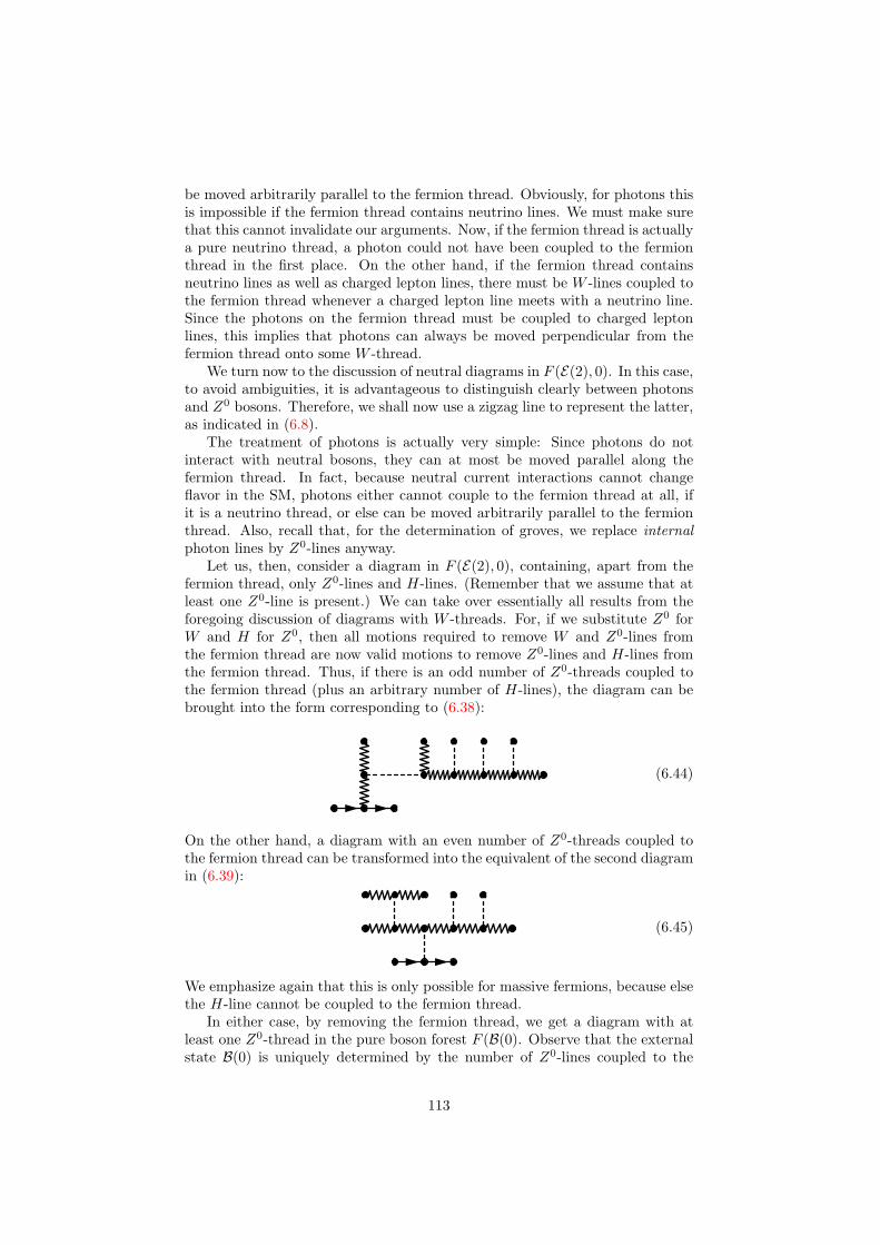
be moved arbitrarily parallel to the fermion thread. Obviously, for photons thisis impossible if the fermion thread contains neutrino lines. We must make surethat this cannot invalidate our arguments. Now, if the fermion thread is actuallya pure neutrino thread, a photon could not have been coupled to the fermionthread in the first place. On the other hand, if the fermion thread containsneutrino lines as well as charged lepton lines, there must be W -lines coupled tothe fermion thread whenever a charged lepton line meets with a neutrino line.Since the photons on the fermion thread must be coupled to charged leptonlines, this implies that photons can always be moved perpendicular from thefermion thread onto some W -thread.

We turn now to the discussion of neutral diagrams in F (E(2), 0). In this case,to avoid ambiguities, it is advantageous to distinguish clearly between photonsand Z0 bosons. Therefore, we shall now use a zigzag line to represent the latter,as indicated in (6.8).

The treatment of photons is actually very simple: Since photons do notinteract with neutral bosons, they can at most be moved parallel along thefermion thread. In fact, because neutral current interactions cannot changeflavor in the SM, photons either cannot couple to the fermion thread at all, ifit is a neutrino thread, or else can be moved arbitrarily parallel to the fermionthread. Also, recall that, for the determination of groves, we replace internalphoton lines by Z0-lines anyway.

Let us, then, consider a diagram in F (E(2), 0), containing, apart from thefermion thread, only Z0-lines and H-lines. (Remember that we assume that atleast one Z0-line is present.) We can take over essentially all results from theforegoing discussion of diagrams with W -threads. For, if we substitute Z0 forW and H for Z0, then all motions required to remove W and Z0-lines fromthe fermion thread are now valid motions to remove Z0-lines and H-lines fromthe fermion thread. Thus, if there is an odd number of Z0-threads coupled tothe fermion thread (plus an arbitrary number of H-lines), the diagram can bebrought into the form corresponding to (6.38):

(6.44)

On the other hand, a diagram with an even number of Z0-threads coupled tothe fermion thread can be transformed into the equivalent of the second diagramin (6.39):

(6.45)

We emphasize again that this is only possible for massive fermions, because elsethe H-line cannot be coupled to the fermion thread.

In either case, by removing the fermion thread, we get a diagram with atleast one Z0-thread in the pure boson forest F (B(0). Observe that the externalstate B(0) is uniquely determined by the number of Z0-lines coupled to the

113

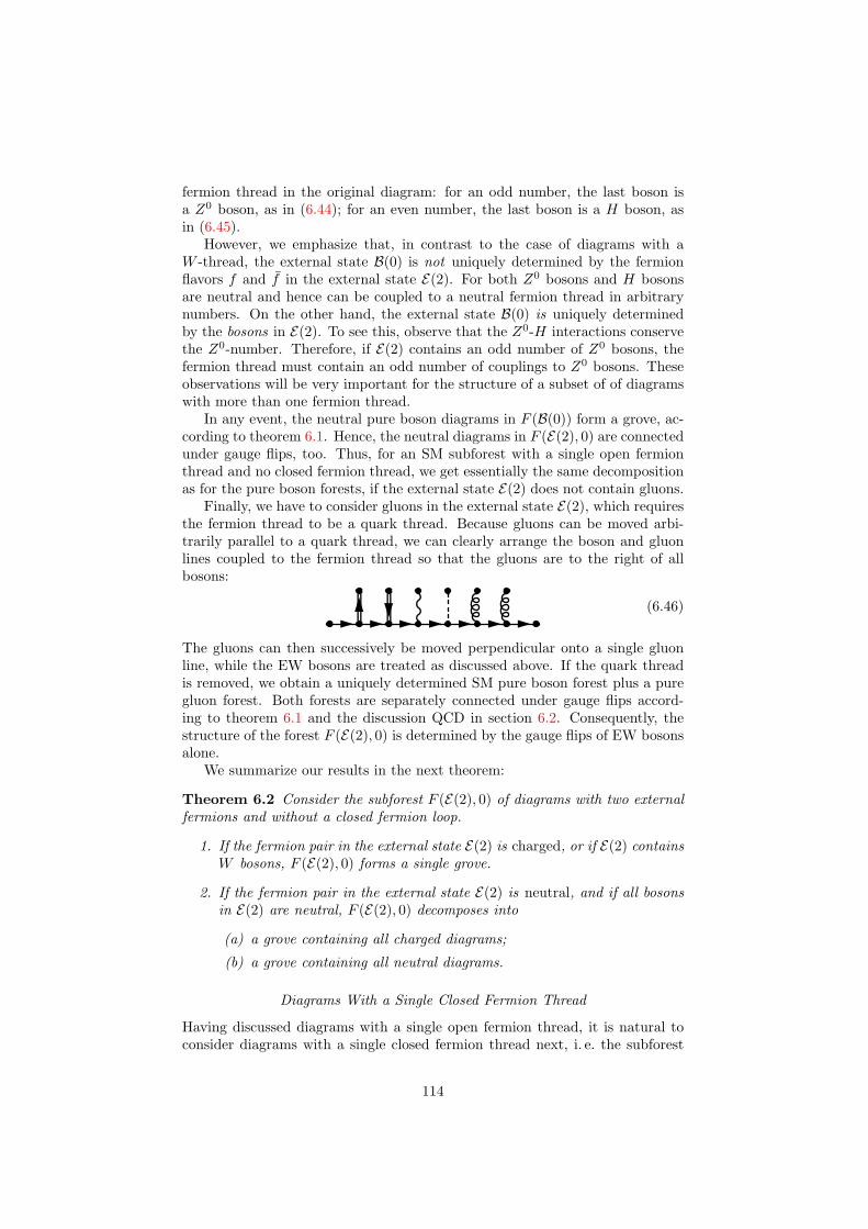
fermion thread in the original diagram: for an odd number, the last boson isa Z0 boson, as in (6.44); for an even number, the last boson is a H boson, asin (6.45).

However, we emphasize that, in contrast to the case of diagrams with aW -thread, the external state B(0) is not uniquely determined by the fermionflavors f and f in the external state E(2). For both Z0 bosons and H bosonsare neutral and hence can be coupled to a neutral fermion thread in arbitrarynumbers. On the other hand, the external state B(0) is uniquely determinedby the bosons in E(2). To see this, observe that the Z0-H interactions conservethe Z0-number. Therefore, if E(2) contains an odd number of Z0 bosons, thefermion thread must contain an odd number of couplings to Z0 bosons. Theseobservations will be very important for the structure of a subset of of diagramswith more than one fermion thread.

In any event, the neutral pure boson diagrams in F (B(0)) form a grove, ac-cording to theorem 6.1. Hence, the neutral diagrams in F (E(2), 0) are connectedunder gauge flips, too. Thus, for an SM subforest with a single open fermionthread and no closed fermion thread, we get essentially the same decompositionas for the pure boson forests, if the external state E(2) does not contain gluons.

Finally, we have to consider gluons in the external state E(2), which requiresthe fermion thread to be a quark thread. Because gluons can be moved arbi-trarily parallel to a quark thread, we can clearly arrange the boson and gluonlines coupled to the fermion thread so that the gluons are to the right of allbosons:

(6.46)

The gluons can then successively be moved perpendicular onto a single gluonline, while the EW bosons are treated as discussed above. If the quark threadis removed, we obtain a uniquely determined SM pure boson forest plus a puregluon forest. Both forests are separately connected under gauge flips accord-ing to theorem 6.1 and the discussion QCD in section 6.2. Consequently, thestructure of the forest F (E(2), 0) is determined by the gauge flips of EW bosonsalone.

We summarize our results in the next theorem:

Theorem 6.2 Consider the subforest F (E(2), 0) of diagrams with two externalfermions and without a closed fermion loop.

1. If the fermion pair in the external state E(2) is charged, or if E(2) containsW bosons, F (E(2), 0) forms a single grove.

2. If the fermion pair in the external state E(2) is neutral, and if all bosonsin E(2) are neutral, F (E(2), 0) decomposes into


(b) a grove containing all neutral diagrams.

Diagrams With a Single Closed Fermion Thread

Having discussed diagrams with a single open fermion thread, it is natural toconsider diagrams with a single closed fermion thread next, i. e. the subforest

114

F (E(0), 1). An external state E(0) without fermions is actually equal to a pureboson external state B. Thus, we are now taking into account the contributionsof diagrams with a single fermion loop to the pure boson forest F (B).

Evidently, the treatment of diagrams with a closed fermion thread is quitesimilar to the treatment of diagrams with an open fermion thread. Indeed, wemade essentially no use of the fact that the fermion thread was open in thediscussion of F (E(2), 0), except that a charged fermion thread must be open.On the other hand, for a neutral open fermion thread, nothing prevents us fromconnecting the end of the thread to the start, thus forming a closed thread.

Observe, that when all but one boson are stripped of a closed neutral fermionthread, the resulting diagram contains a one-loop tadpole diagram contributingto the one-point function of some neutral boson:

(6.47)

Such a tadpole diagram is zero by Lorentz invariance for the neutral gaugebosons, i. e. photon and Z0, because the corresponding integral would, if nonzero,define a preferred four-momentum:

γ,Z0

= 0 (6.48)

However, the Goldstone boson and H tadpole diagrams are generally nonzerofor massive fermions. In fact they are proportional to the fermion masses.Therefore, we can really take over all arguments from the case of a closed fermionthread and obtain the following result:

Theorem 6.3 Consider the subforest F (E(0), 1) of diagrams without externalfermions and with a single closed fermion loop. F (E(0), 1) decomposes into

1. a grove containing all charged diagrams;

2. a grove containing all neutral diagrams.

General SM Diagrams

We are now in a position to study general SM forests, i. e. diagrams with anarbitrary number of fermion threads, open or closed. As we have seen above,closed fermion threads can be treated in the same way as open ones. Therefore,it suffices to consider diagrams with a fixed number of fermion threads. Sinceno gauge flip can change the number of fermion threads, this is automaticallycompatible with gauge invariance.

Denote by F (E , τ) a forest of diagrams with τ fermion threads and an ex-ternal state E , which is only subject to the constraint that it must not containmore than 2τ fermions. The τ fermion threads can be assumed to belong mu-tually distinct fermion dublets. For, if some fermion threads belong to identicaldublets, the complete forest will decompose into invariant subsets related toeach other by permutations of fermion threads and crossing symmetry.

For instance, take F (E , 3) to be the forest of diagrams without fermion loopfor the SM process e+e− → e+e−µ+µ− at one-loop level. For every diagram

115

d1 contributing to this process, there is a second diagram d2 related to d1 by apermutation of external electron lines, i. e. by crossing symmetry. A priori bothd1 and d2 might belong to a single grove of the forest for this process. However,the e+-e− pair in the final state could have been replaced by a quark-antiquarkpair without violating gauge invariance, in which case no permutation of externallines would be possible. Consequently, d1 and d2 must belong to different grovesS1 and S2, related to each other by crossing symmetry.

Given that all fermion threads belong to distinct fermion dublets, our strat-egy for determining the structure of the subforest F (τ) will be as follows: Leav-ing QCD couplings aside, we first consider external states E without photons.For such external states, we can remove all but one boson from every fermionthread. This should be clear, because we just have to treat each fermion threadin turn like we did above. Removing afterwards the trivial fermion threads willgive us a diagram from a pure boson forest F (B) with a bosonic external stateB. The structure of F (τ) then follows from the structure of the pure bosonforest, which, according to theorem 6.1, is characterized by the bosonic externalstate B. Once we have derived the structure of the forest for an external stateE without photons, the effects of adding the latter gauge bosons can easily bedetermined.

Consider, then, an external state E without photons. If E contains W bosonsor charged external fermion pairs, the last boson kept at each fermion threadis uniquely determined, if we demand that the last boson at all neutral fermionthreads be a Z0 (or φ0, for closed fermion threads). This is true because thesediagrams contain open W -threads, to which all neutral bosons can eventually beattached. But a H-line coupled to a W -thread can always be eliminated in favorof a Z0-line or φ0-line. Consequently, the external state B of the pure bosonforest obtained by removing the stripped fermion threads is uniquely determinedand contains external W bosons. According to theorem 6.1, F (B) is connectedin this case. Therefore, F (E , τ) is connected, too. The same is true if photonsare added to the original external state E , because these can always be movedonto some W -thread. Thus, adding external photons just changes the purelybosonic external state B.

If no W bosons or charged fermion pairs are present in the original exter-nal state E , the forest F (E , τ) decomposes into the invariant subsets containingcharged and neutral diagrams, respectively. The subset of charged diagrams is,in fact, a grove, which follows again from the uniqueness of the purely bosonic ex-ternal state B obtained by first stripping and then removing all fermion threads.Theorem 6.1 then ensures the connectedness of the charged diagrams. Again,photons can be added to E without invalidating this result, because they maybe attached to a W -thread.

Thus, independent of the external state E , the charged diagrams in F (E , τ)always form a single grove.

We turn now to the discussion of neutral diagrams. Of course, for these toexist, the external state E must not contain charged bosons or fermion pairs.This will be implicitely understood in the sequel. Because, even with theseconstraints, there are still charged diagrams in F (E , τ), we denote the subset ofneutral diagrams as F0(E , τ).

Let E again denote an external state without photons. For each diagram inF0(E , τ), we can remove all but one boson from open fermion threads. Once wehave done this, removing the open fermion threads gives us a purely bosonic

116

external state B containing H and Z0 bosons only. This time, however, B isnot uniquely determined. To see this, observe that, since all fermion threads indiagrams of F0(E , τ) are neutral, the last boson at each fermion thread must beeither a H or a Z0 (or φ0). However, in a neutral diagram there is no way toreplace a H-line by a Z0-line.

Indeed, in a neutral diagram, an internal H-line must either connect twofermion threads or else be coupled to at least one HZ0Z0 or HHH-vertex. Inthe latter case, the absence of a HHZ0 or a Z0Z0Z0-vertex in the SM forbidsthe replacement of aH-line. In the former case, a replacement would in principlebe possible. It is, however, not a gauge motion, because the exchange of H-lineand Z0-line in a four-point subdiagram with four fermion lines is not a gaugeflip:

/↔ (6.49)

Therefore, different ways of choosing the last boson at each fermion thread,corresponding to different pure boson external states B obtained by strippingand removing the fermion threads, lead to separate groves. Thus, in order todetermine the groves of F0(E , τ), we must determine all possible pure bosonexternal states B.

For instance, consider F0(E , 3) for an external state E containing three dis-tinct neutral fermion pairs at the one-loop order. A specific example is providedby the SM process e+e− → e+e−µ+µ− described above. In this case, we haveto take into account all pure boson external states B consisting of three neutralbosons, each either a Z0 or a H. Because the Z0-H interactions conserve the Z0

number, B must contain either zero or two Z0 bosons. For the latter possibility,there are three choices, characterized by specifying the fermion threads to whichthe Z0-lines are attached. We illustrate this by displaying one representativediagram for each choice of external state:

(6.50)Evidently, the four choices of external state B are independent of the number ofloops, as long as we do not introduce a fermion loop (which would be equivalentto changing τ). This is true because, according to 6.1, the neutral pure bosongroves are uniquely determined by the external state B for any number of loops.

It is also easy to extend the original external state E by adding H bosonsor pairs of Z0 bosons, because these can always be attached to one of the Z0-threads already present in the pure boson part of the diagram. The groves wouldthen still be characterized by the four choices of last boson at the three fermionthreads. On the other hand, if we wanted to add just a single Z0 boson to theexternal state E , we would have to choose an odd number of fermion threadsfor which the last boson is a Z0.

117

In any event, the foregoing discussion shows that in F0(E , τ) there are gen-erally several independent choices of last boson at the τ fermion threads. Eachchoice leads to a different pure boson external state B and hence to a separategrove. Alternatively, because the number modulo two of Z0 bosons at a fermionthread is determined uniquely by the choice of last boson, we can characterizethe groves of F0(E , τ) by these numbers. This will be illustrated further whenwe discuss an explicit example later.

We summarize what we have learned about the subforest F0(E , τ) of neutraldiagrams without external photons in a lemma:

Lemma 6.1 The forest F0(E , τ) of neutral diagrams with τ fermion threadsdecomposes into one grove for every independent choice of last boson at the τfermion threads. If the number of external Z0 bosons is even or odd, thesechoices correspond to all possible ways of selecting an even or odd number offermion threads, respectively, for which the last boson is a Z0.

Adding external photons will in general lead to a further decomposition ofF0(E , τ). To see this, observe that, while photons can be moved parallel toa fermion thread, it is impossible to remove a photon from a fermion thread ina diagram containing only neutral bosons through gauge motions, simply be-cause there is no charged boson to which the photon could be attached. Thismeans that we cannot transfer photons from one fermion thread to another bygauge flips.

Therefore, if photons are added to the external state E , the groves describedin the lemma will decompose further into one grove for every independent wayof distributing the photons over the fermion threads.

As a simple example, consider the process e+e− → µ+µ−γ at tree level.Ignoring the photon, there are two choices of last boson at the fermion threads,corresponding to Z0-exchange or H-exchange. For both choices, we can attachthe photon to the electron line or the muon line. Consequently, the forest forthis process decomposes into four groves: , , ,

(6.51)

, , ,

(6.52)

,

(6.53)

118

,

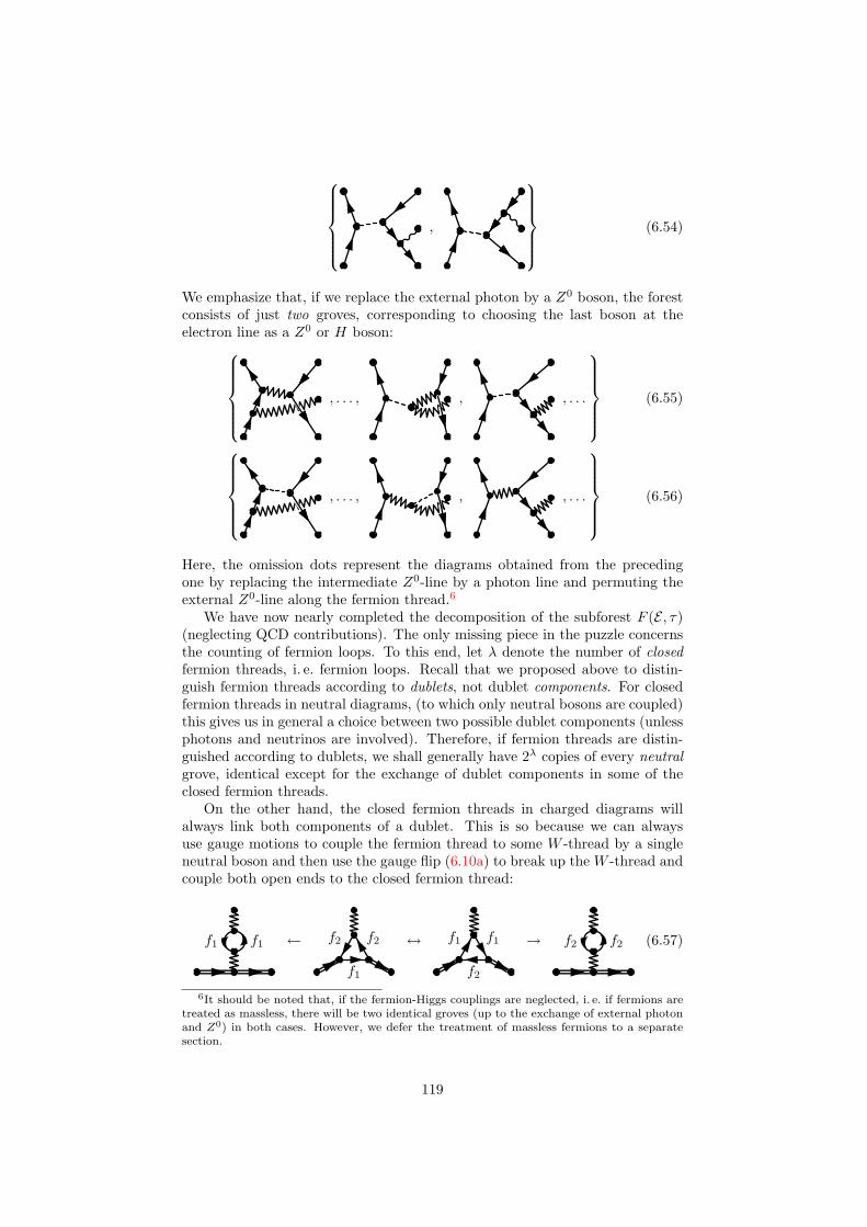
(6.54)

We emphasize that, if we replace the external photon by a Z0 boson, the forestconsists of just two groves, corresponding to choosing the last boson at theelectron line as a Z0 or H boson: , . . . , , , . . .

(6.55)

, . . . , , , . . .

(6.56)

Here, the omission dots represent the diagrams obtained from the precedingone by replacing the intermediate Z0-line by a photon line and permuting theexternal Z0-line along the fermion thread.6

We have now nearly completed the decomposition of the subforest F (E , τ)(neglecting QCD contributions). The only missing piece in the puzzle concernsthe counting of fermion loops. To this end, let λ denote the number of closedfermion threads, i. e. fermion loops. Recall that we proposed above to distin-guish fermion threads according to dublets, not dublet components. For closedfermion threads in neutral diagrams, (to which only neutral bosons are coupled)this gives us in general a choice between two possible dublet components (unlessphotons and neutrinos are involved). Therefore, if fermion threads are distin-guished according to dublets, we shall generally have 2λ copies of every neutralgrove, identical except for the exchange of dublet components in some of theclosed fermion threads.

On the other hand, the closed fermion threads in charged diagrams willalways link both components of a dublet. This is so because we can alwaysuse gauge motions to couple the fermion thread to some W -thread by a singleneutral boson and then use the gauge flip (6.10a) to break up the W -thread andcouple both open ends to the closed fermion thread:

f1f1 ←

f1

f2f2 ↔ f1

f2

f1 → f2f2 (6.57)

6It should be noted that, if the fermion-Higgs couplings are neglected, i. e. if fermions aretreated as massless, there will be two identical groves (up to the exchange of external photonand Z0) in both cases. However, we defer the treatment of massless fermions to a separatesection.

119

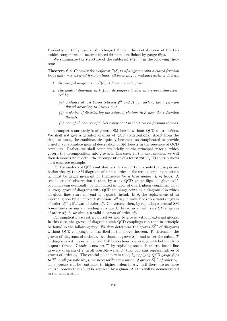
Evidently, in the presence of a charged thread, the contributions of the twodublet components in neutral closed fermions are linked by gauge flips.

We summarize the structure of the subforest F (E , τ) in the following theo-rem:

Theorem 6.4 Consider the subforest F (E , τ) of diagrams with λ closed fermionloops and τ−λ external fermion lines, all belonging to mutually distinct dublets.

1. All charged diagrams in F (E , τ) form a single grove.

2. The neutral diagrams in F (E , τ) decompose further into groves character-ized by

(a) a choice of last boson between Z0 and H for each of the τ fermionthread according to lemma 6.1;

(b) a choice of distributing the external photons in E over the τ fermionthreads;

(c) one of 2λ choices of dublet component in the λ closed fermion threads.

This completes our analysis of general SM forests without QCD contributions.We shall not give a detailed analysis of QCD contributions. Apart from thesimplest cases, the combinatorics quickly becomes too complicated to providea useful yet complete general description of SM forests in the presence of QCDcouplings. Rather, we shall comment briefly on the principal criteria, whichgovern the decomposition into groves in this case. In the next section, we willthen demonstrate in detail the decomposition of a forest with QCD contributionson a concrete example.

For the analysis of QCD contributions, it is important to note that, in pertur-bation theory, the SM diagrams of a fixed order in the strong coupling constantαs must be gauge invariant by themselves for a fixed number L of loops. Asecond crucial observation is that, by using QCD gauge flips, all gluon self-couplings can eventually be eliminated in favor of quark-gluon couplings. Thatis, every grove of diagrams with QCD couplings contains a diagram d in whichall gluon lines start and end at a quark thread. In d, the replacement of aninternal gluon by a neutral EW boson, Z0 say, always leads to a valid diagramof order αn−1

s , if d was of order αns . Conversely, then, by replacing a neutral SM

boson line starting and ending at a quark thread in an arbitrary SM diagramof order αn−1

s , we obtain a valid diagram of order αns .

For simplicity, we restrict ourselves now to groves without external gluons.In this case, the groves of diagrams with QCD couplings can then in principlebe found in the following way: We first determine the groves S(0)

i of diagramswithout QCD couplings, as described in the above theorem. To determine thegroves of diagrams of order αs, we choose a grove S(0)

i and select the subset Tof diagrams with internal neutral EW boson lines connecting with both ends toa quark thread. Obtain a new set T ′ by replacing one such neutral boson linein every diagram of T in all possible ways. T ′ then contains representatives ofgroves of order αs. The crucial point now is that, by applying QCD gauge flipsto T ′ in all possible ways, we necessarily get a union of groves S(1)

k of order αs.This process can be continued to higher orders in αs, until there are no moreneutral bosons that could be replaced by a gluon. All this will be demonstratedin the next section.

120

While the procedure just described gives us a way to construct the grovesof diagrams with QCD couplings, it does not actually characterize these groves.We will now make some general remarks about the characterization of groveswith QCD couplings. Suppose, then, that we want to classify the groves of orderαs. A diagram of order αs contains a single gluon, which can either connect twodifferent quark threads or couple to a single quark thread. The groves are thendistinguished at least by the choices of two or one quark thread, respectively.In most cases, there will be further choices associated with the couplings ofEW bosons to the quark threads. We shall demonstrate this explicitely for asufficiently simple, yet nontrivial, example in the next section.

In a similar way, one can in principle characterize the groves of higher or-ders in αs. However, the combinatorics required for devising a general schemebecomes forbiddingly complicated. On the other hand, the formalism of flips isideally suited for an implementation in a computer program. We have imple-mented the algorithm for the construction of groves of the SM. The results willbe presented later. However, in order to make a connection with our theoreticaldiscussion, we shall demonstrate the decomposition of the forest into groves onan explicit example, which we shall then analyze by means of our computerprogram.

6.3.5 Structure of SM Forests: An Explicit Example

We have now all the information at hand which is needed to decompose a generalSM forest into its groves. Instead of describing the general procedure, whichwould soon become very awkward, we shall discuss a specific example illustratingthe essential steps. Our arguments will also be applicable in the general case.For simplicity, we specialize to the one-loop case, i. e. L = 1.

Consider, then, the connected Green’s function G for the process e+e− →uudd. The complete forest of all one-loop diagrams contributing to G, includingQCD contributions, will be denoted as F . The invariant subsets of diagrams oforder α0

s, α1s, and α2

s are referred to as F (0), F (1), and F (2), respectively.

Purely Electroweak Contributions

We shall first treat the forest F (0) of diagrams without QCD couplings, takingaccount of QCD contributions later. There are two ways of associating theexternal fermions to fermion threads, corresponding to the groupings (u, u) and(d, d) or (u, d) and (d, u), respectively. In other words, the forest of one-loopdiagrams of G decomposes into two invariant subsets F (0)

(En)

and F (0)(Ec),

characterized by the external states

En =(e+, e−), (u, u), (d, d)

(6.58)

Ec =(e+, e−), (u, d), (d, u)

. (6.59)

F (0)(En)

and F (0)(Ec)

can be further decomposed according to the numberλ of fermion loops, which can be 0 or 1. For λ = 0, we denote the subsets asF (0)

(En, 0

)and F (0)

(Ec, 0

), respectively. For λ = 1, we characterize the fermion

loop by the fermion dublet, f , in the case of Ec, or by the dublet component,fk, in the case of En, writing, respectively, F (0)

(En, fk

)or F (0)

(Ec, f

).

Before going into the details of the decomposition, we have to say that itwould be too much to display the complete groves. However, since groves are

121

equivalence classes of diagrams under gauge flips, we can display a representativefor each grove, using brackets to denote the respective equivalence class. Thus,if d is a diagram in a grove S, we write S = [d]. In the next section, we willthen report the sizes of these groves as we have obtained them by means of ourcomputer program.

We begin with the decomposition of F (0)(Ec). All diagrams in this subset

are charged, because the external state Ec contains charged fermion threads.According to theorem 6.4, the charged diagrams without fermion F (0)

(Ec, 0

)loop form a single grove:

F (0)(Ec, 0

)=

e+

e−

d

d

u

u

(6.60)

Note that this diagrams is the same as (1.3), which we choose to illustrate theaction of gauge flips in the introduction. Therefore, any of the diagrams inchapter 1 could have been used as a representative for this grove.

The diagrams with a single fermion loop form one grove F (0)(Ec, f) for eachfermion dublet f :

F (0)(Ec, f

)=

f

e+

e−

d

d

u

u

(6.61)

The subset F (0)(En, 0

)contains, according to theorem (6.4), a charged grove

F(0)+

(En, 0

):

F(0)+

(En, 0

)=

e+

e−

d

d

u

u

(6.62)

We have now exhausted all charged diagrams. Indeed, a diagram in F (0)(En, fk

)cannot contain a W -thread, because in a diagram with a neutral external statethe W -thread must be part of a loop. However, the only loop in F (0)

(En, fk

)is

a closed fermion thread, hence there is no room for a W -thread.

122

The invariant subset F (0)0

(En, 0

)of neutral diagrams in F (0)

(En, 0

)decom-

poses, according to theorem 6.4, into neutral groves according to the number(modulo two) of Z0 bosons coupled to each fermion thread. We have illustratedthese choices for the case at hand as an example in (6.50). Thus, there are fourgroves, which we characterize by specifying the flavors of the fermion threadsto which an odd number of Z0 bosons is coupled. We display three of these:

F(0)0

(En, 0; 0

)=

e+

e−

d

d

u

u

(6.63)

F(0)0

(En, 0;u, d

)=

e+

e−

d

d

u

u

(6.64)

F(0)0 (En, 0; e, u) =

e+

e−

d

d

u

u

(6.65)

The representative for the remaining grove F (0)0

(En, 0; e, d

)is obtained by per-

muting u and d in an obvious way.In a similar manner, the neutral groves in F (0)

(En, fk

)decompose into neu-

tral groves, which can again be characterized by specifying the flavor of thefermion threads to which have an odd number of couplings to Z0 bosons. First,there is the grove F (0)

(En, fk; e, u, d, (fk)

)corresponding to an odd number of

Z0 couplings at every fermion thread:

F (0)(En, fk; e, u, d, (fk)

)=

fk

e+

e−

d

d

u

u

(6.66)

Here, the fermion propagating in the loop has been put into extra parenthesesto distinguish it from the external fermions.

123

Then, we can choose an odd number of Z0 couplings at just two fermionthreads, which may be either two external fermion threads or one external threadand the loop. We display one choice for both cases (the notation should beevident by now):

F (0)(En, fk;u, d

)=

fk

e+

e−

d

d

u

u

(6.67)

F (0)(En, fk; e, (fk)

)=

fk

e+

e−

d

d

u

u

(6.68)

The other four choices lead to the groves F (0)(En, fk; e, u

)and F (0)

(En, fk; e, d

)on one hand as well as F (0)

(En, fk;u, (fk)

)and F (0)

(En, fk; d, (fk)

)on the other

hand.This completes the decomposition of the forest for the Green’s function G.

Let us briefly summarize the groves, neglecting trivial groves of diagrams with-out gauge bosons, and restricting ourselves to a simplified version of the SMwith just one generation of fermions, i. e. the leptons e and ν as well as thequarks u and d. There is no loss of generality in this restriction, because, aswe have argued above, the groves of the complete SM can be obtained from theone-generation SM by merely exchanging flavors in the fermion loops.

First, we have the groves without fermion loop, which are the two chargedgroves F (0)

(Ec, 0

)and F

(0)+

(En, 0

)as well as the neutral groves F (0)

0

(En, 0; 0

)plus three groves F (0)

0

(En, 0; t1, t2

), where t1 and t2 refer to the open fermion

threads. Thus, there are six groves without fermion loop. The groves withfermion loop are given by two copies of the charged grove F (0)

(Ec, f

), one each

for the two dublets, and four copies each of F (0)(En, fk; e, n, d, (fk)

), of the three

choices F (0)(En, fk; t1, t2

), and of the three choices F (0)

(En, fk; t, (fk)

)(where t

again refers to the three open fermion threads), one for each of the four dubletcomponents. All in all, this makes up for 36 nontrivial groves.

Of course, the forest of G, as we have discussed it, is not really equal tothe set of diagrams from which G would be computed in practice. For, at themoment we include Higgs couplings to all SM fermions, whereas, for practicalpurposes, the couplings of light fermions to the Higgs can often be ignored. Wewill discuss the implications of treating fermions as massless below. Here, wejust make two general remarks. First, the structure of the charged groves isnot affected by treating fermions as massless. This is intuitively clear, becauseinternal H-lines can always be eliminated in a diagram with W -thread. Second,

124

treating fermions as massless will usually lead to a further decomposition ofsome neutral groves for massive fermions, although other neutral groves may becompletely absent. Also, we have to say something about QCD contributions.We will take up these issues below.

Before we do that, however, we want to briefly comment on the impact onthe structure of the forest brought about by adding an external photon. Thatis, we consider now the process e+e− → uuddγ. The corresponding externalstates external states E ′n and E ′c are then given by including the extra photon inEn and Ec, respectively:

E ′n =(e+, e−), (u, u), (d, d), γ

(6.69)

E ′c =(e+, e−), (u, d), (d, u), γ

. (6.70)

According to theorem 6.4, the structure of charged groves is unaffected by theadditional photon. For instance, the grove F (0)

(E ′c, 0

)is obtained by adding the

photon in all diagrams of F (0)(Ec, 0

)in all possible places.

On the other hand, adding the photon to a neutral grove will lead to severalseparate groves, one for each choice of fermion thread to which the photon canbe attached. We illustrate this for the neutral grove F (0)

(E ′n, fk;u, d

), charac-

terizing the four groves by the flavor of the fermion thread to which the photonis attached:

F (0)(E ′n, fk;u, d; e

)=

fk

e+

e−

d

d

u

u

(6.71)

F (0)(E ′n, fk;u, d;u

)=

fk

e+

e−

d

d

u

u

(6.72)

F (0)(E ′n, fk;u, d; d

)=

fk

e+

e−

d

d

u

u

(6.73)

125

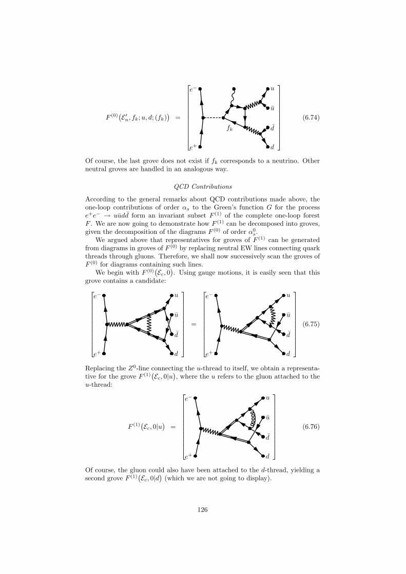
F (0)(E ′n, fk;u, d; (fk)

)=

fk

e+

e−

d

d

u

u

(6.74)

Of course, the last grove does not exist if fk corresponds to a neutrino. Otherneutral groves are handled in an analogous way.

QCD Contributions

According to the general remarks about QCD contributions made above, theone-loop contributions of order αs to the Green’s function G for the processe+e− → uudd form an invariant subset F (1) of the complete one-loop forestF . We are now going to demonstrate how F (1) can be decomposed into groves,given the decomposition of the diagrams F (0) of order α0

s.We argued above that representatives for groves of F (1) can be generated

from diagrams in groves of F (0) by replacing neutral EW lines connecting quarkthreads through gluons. Therefore, we shall now successively scan the groves ofF (0) for diagrams containing such lines.

We begin with F (0)(Ec, 0

). Using gauge motions, it is easily seen that this

grove contains a candidate:e+

e−

d

d

u

u

=

e+

e−

d

d

u

u

(6.75)

Replacing the Z0-line connecting the u-thread to itself, we obtain a representa-tive for the grove F (1)

(Ec, 0|u

), where the u refers to the gluon attached to the

u-thread:

F (1)(Ec, 0|u

)=

e+

e−

d

d

u

u

(6.76)

Of course, the gluon could also have been attached to the d-thread, yielding asecond grove F (1)

(Ec, 0|d

)(which we are not going to display).

126

This does not yet exhaust the groves obtained from F (0)(Ec, 0

), because

there is also a representative with a Z0-line connecting both quark threads:e+

e−

d

d

u

u

=

e+

e−

d

d

u

u

(6.77)

Replacing the Z0-line here gives us a third grove F (1)(Ec, 0|u, d

):

e+

e−

d

d

u

u

(6.78)

Since the general principle should by now be clear, we shall no longer display theoriginal representatives and candidates. Rather, we display the representativefrom F (1) directly. The candidate can be inferred from this representative in anobvious way by replacing the gluon with a Z0 or H-line.

Two further charged groves can be constructed from F(0)+

(En, 0

). We display

the first one:

F(1)+

(En, 0|u

)=

e+

e−

d

d

u

u

(6.79)

The second grove, F (1)+

(En, 0|d

)is obtained in an obvious way by attaching the

Z0-line to the d-thread instead of the u-thread. This exhausts the list of chargedgroves, because in F (0)

(Ec, f

)there are no candidate diagrams.

Let us, then, turn to neutral diagrams. There, we can replace a Z0-linebetween quark threads by a gluon line, which can be part of the loop or not.In the former case, we obtain three groves from each of F (0)

0

(En, 0; t1, t2

). For

127

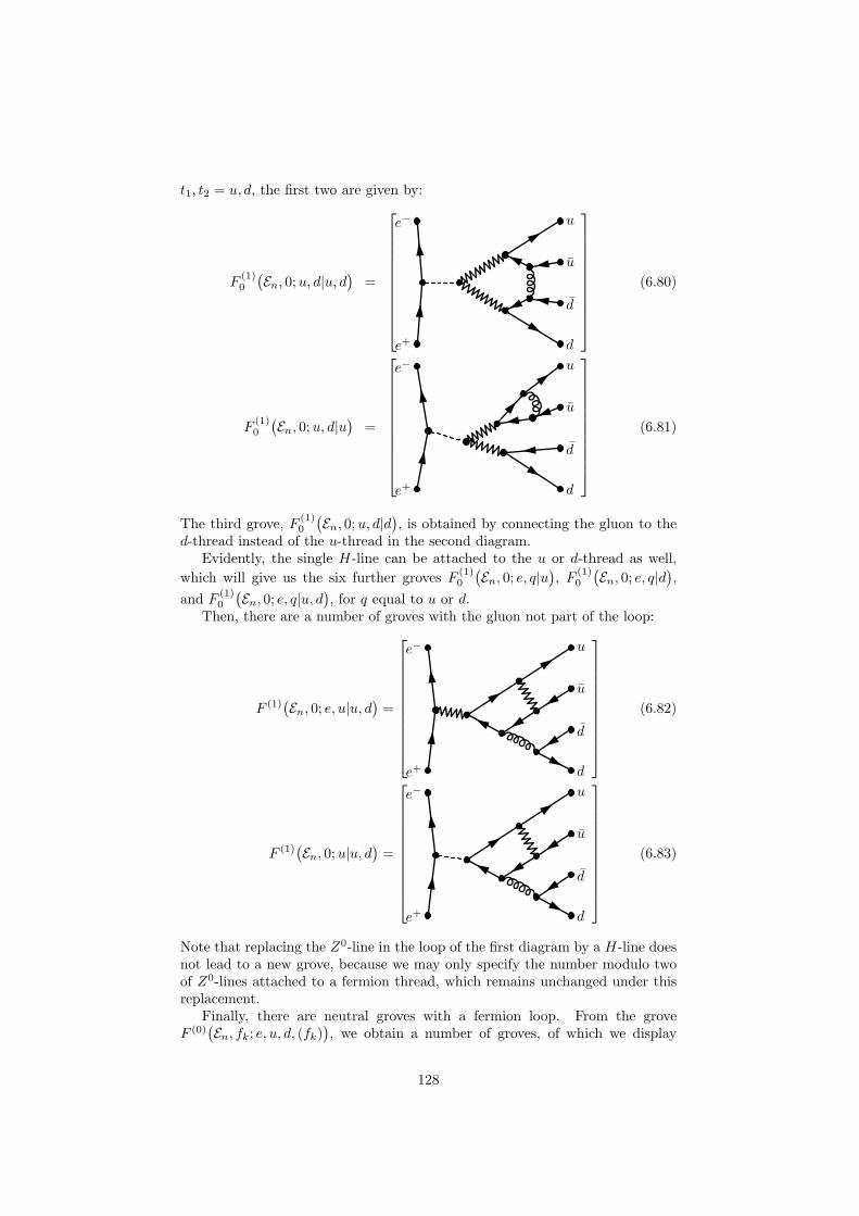
t1, t2 = u, d, the first two are given by:

F(1)0

(En, 0;u, d|u, d

)=

e+

e−

d

d

u

u

(6.80)

F(1)0

(En, 0;u, d|u

)=

e+

e−

d

d

u

u

(6.81)

The third grove, F (1)0

(En, 0;u, d|d

), is obtained by connecting the gluon to the

d-thread instead of the u-thread in the second diagram.Evidently, the single H-line can be attached to the u or d-thread as well,

which will give us the six further groves F (1)0

(En, 0; e, q|u

), F (1)

0

(En, 0; e, q|d

),

and F (1)0

(En, 0; e, q|u, d

), for q equal to u or d.

Then, there are a number of groves with the gluon not part of the loop:

F (1)(En, 0; e, u|u, d

)=

e+

e−

d

d

u

u

(6.82)

F (1)(En, 0;u|u, d

)=

e+

e−

d

d

u

u

(6.83)

Note that replacing the Z0-line in the loop of the first diagram by a H-line doesnot lead to a new grove, because we may only specify the number modulo twoof Z0-lines attached to a fermion thread, which remains unchanged under thisreplacement.

Finally, there are neutral groves with a fermion loop. From the groveF (0)


), we obtain a number of groves, of which we display

128

some explicitely:

F (1)(En, fk; e, (fk)|u, d

)=

fk

e+

e−

d

d

u

u

(6.84)

F (1)(En, qk; e, (qk), u, d|u, qk

)=

qk

e+

e−

d

d

u

u

(6.85)

F (1)(En, qk; e, d|u, qk

)=

qk

e+

e−

d

d

u

u

(6.86)

Here, qk refers to the component of a quark multiplet. The further grovesobtained from F (0)


)correspond to permuting u and d-thread

in the above diagrams. Observe that some of these groves can also be obtainedfrom other groves of F (0). For instance, the grove F (1)(En, qk; e, d|u, qk) canalso be obtained from F (0)(En, hk; e, d), by replacing a H-line with a gluon.This does not contradict our general remark that a grove in F (0) is turned intoa union of groves in F (1) when all possible replacements and QCD gauge flips areperformed, because we did not claim that the groves in F (1) would be differentfor different original groves in F (0).

The remaining neutral groves in F (1) are similar in structure to the threeones displayed last, with Z0-lines replaced by H-lines, and vice versa, in allpossible ways. This completes the construction of the groves of F (1). Lookingback at the representatives for these groves, it is apparent that these can indeedbe characterized by specifying the quark threads to which the gluon is attached,and, in addition, to which fermion threads the EW bosons are coupled. Wehave used this fact in an intuitive way to denote the groves in F (1).

We shall not analyze the subset F (2) of order α2s in the same detail. The con-

struction of the groves can be performed in an analogous way. Instead, we justdisplay example representatives for all occuring structures (without introducing

129

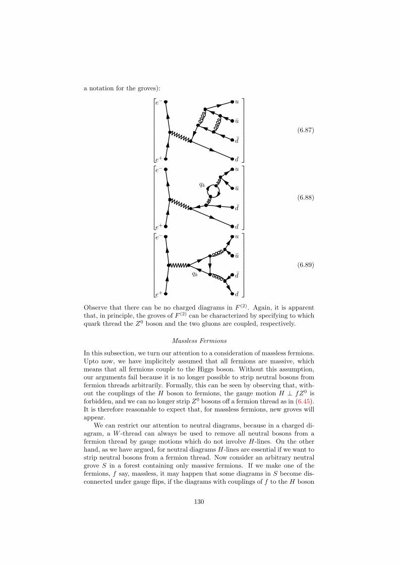
a notation for the groves):e+

e−

d

d

u

u

(6.87)

qk

e+

e−

d

d

u

u

(6.88)

qk

e+

e−

d

d

u

u

(6.89)

Observe that there can be no charged diagrams in F (2). Again, it is apparentthat, in principle, the groves of F (2) can be characterized by specifying to whichquark thread the Z0 boson and the two gluons are coupled, respectively.

Massless Fermions

In this subsection, we turn our attention to a consideration of massless fermions.Upto now, we have implicitely assumed that all fermions are massive, whichmeans that all fermions couple to the Higgs boson. Without this assumption,our arguments fail because it is no longer possible to strip neutral bosons fromfermion threads arbitrarily. Formally, this can be seen by observing that, with-out the couplings of the H boson to fermions, the gauge motion H ⊥ fZ0 isforbidden, and we can no longer strip Z0 bosons off a fermion thread as in (6.45).It is therefore reasonable to expect that, for massless fermions, new groves willappear.

We can restrict our attention to neutral diagrams, because in a charged di-agram, a W -thread can always be used to remove all neutral bosons from afermion thread by gauge motions which do not involve H-lines. On the otherhand, as we have argued, for neutral diagrams H-lines are essential if we want tostrip neutral bosons from a fermion thread. Now consider an arbitrary neutralgrove S in a forest containing only massive fermions. If we make one of thefermions, f say, massless, it may happen that some diagrams in S become dis-connected under gauge flips, if the diagrams with couplings of f to the H boson

130

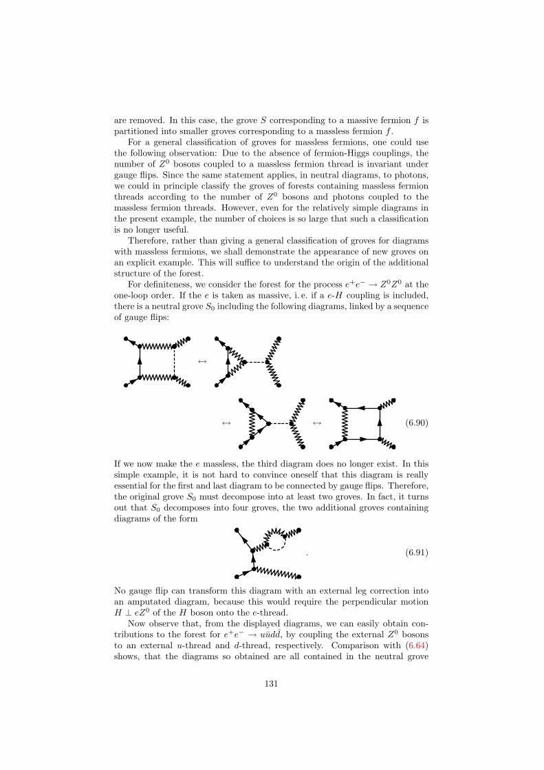
are removed. In this case, the grove S corresponding to a massive fermion f ispartitioned into smaller groves corresponding to a massless fermion f .

For a general classification of groves for massless fermions, one could usethe following observation: Due to the absence of fermion-Higgs couplings, thenumber of Z0 bosons coupled to a massless fermion thread is invariant undergauge flips. Since the same statement applies, in neutral diagrams, to photons,we could in principle classify the groves of forests containing massless fermionthreads according to the number of Z0 bosons and photons coupled to themassless fermion threads. However, even for the relatively simple diagrams inthe present example, the number of choices is so large that such a classificationis no longer useful.

Therefore, rather than giving a general classification of groves for diagramswith massless fermions, we shall demonstrate the appearance of new groves onan explicit example. This will suffice to understand the origin of the additionalstructure of the forest.

For definiteness, we consider the forest for the process e+e− → Z0Z0 at theone-loop order. If the e is taken as massive, i. e. if a e-H coupling is included,there is a neutral grove S0 including the following diagrams, linked by a sequenceof gauge flips:

↔

↔ ↔ (6.90)

If we now make the e massless, the third diagram does no longer exist. In thissimple example, it is not hard to convince oneself that this diagram is reallyessential for the first and last diagram to be connected by gauge flips. Therefore,the original grove S0 must decompose into at least two groves. In fact, it turnsout that S0 decomposes into four groves, the two additional groves containingdiagrams of the form

. (6.91)

No gauge flip can transform this diagram with an external leg correction intoan amputated diagram, because this would require the perpendicular motionH ⊥ eZ0 of the H boson onto the e-thread.

Now observe that, from the displayed diagrams, we can easily obtain con-tributions to the forest for e+e− → uudd, by coupling the external Z0 bosonsto an external u-thread and d-thread, respectively. Comparison with (6.64)shows, that the diagrams so obtained are all contained in the neutral grove

131

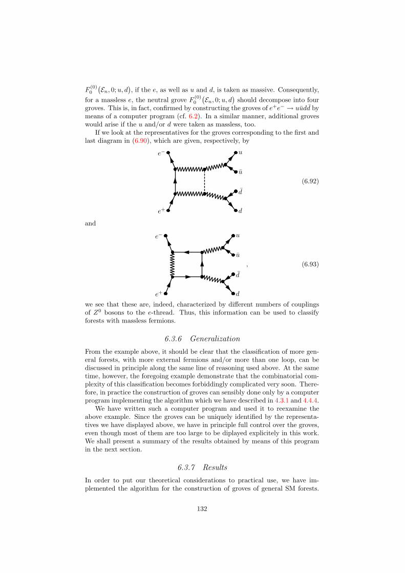
F(0)0

(En, 0;u, d

), if the e, as well as u and d, is taken as massive. Consequently,

for a massless e, the neutral grove F (0)0

(En, 0;u, d

)should decompose into four

groves. This is, in fact, confirmed by constructing the groves of e+e− → uudd bymeans of a computer program (cf. 6.2). In a similar manner, additional groveswould arise if the u and/or d were taken as massless, too.

If we look at the representatives for the groves corresponding to the first andlast diagram in (6.90), which are given, respectively, by

e+

e−

d

d

u

u

(6.92)

and

e+

e−

d

d

u

u

, (6.93)

we see that these are, indeed, characterized by different numbers of couplingsof Z0 bosons to the e-thread. Thus, this information can be used to classifyforests with massless fermions.

6.3.6 Generalization

From the example above, it should be clear that the classification of more gen-eral forests, with more external fermions and/or more than one loop, can bediscussed in principle along the same line of reasoning used above. At the sametime, however, the foregoing example demonstrate that the combinatorial com-plexity of this classification becomes forbiddingly complicated very soon. There-fore, in practice the construction of groves can sensibly done only by a computerprogram implementing the algorithm which we have described in 4.3.1 and 4.4.4.

We have written such a computer program and used it to reexamine theabove example. Since the groves can be uniquely identified by the representa-tives we have displayed above, we have in principle full control over the groves,even though most of them are too large to be diplayed explicitely in this work.We shall present a summary of the results obtained by means of this programin the next section.

6.3.7 Results

In order to put our theoretical considerations to practical use, we have im-plemented the algorithm for the construction of groves of general SM forests.

132

e+e− → uudd (L = 1) mf 6= 0 mν = 0 me = 0 mq = 0

O(α0s)

Number of Diagrams 58382 54272 18713 4233Gauge Groves 36 36 45 57Pure Higgs Groves 601 520 0 0

O(α1s)


O(α2s)


Table 6.1: Total number of diagrams (omitting diagrams with ghost loops)and number of groves for the one-loop corrections to e+e− → uudd in a one-generation SM, according to the number of fermions treated as massless. Detailsare explained in the text.

In this section, we will present the results obtained for the one-loop forest ofthe process e+e− → uudd, which we have discussed in much detail in the lastsection.

For the sake of simplicity, we have again restricted the SM to one fermiongeneration. Furthermore, we have omitted diagrams with ghosts. As we haveshown in chapter 4, the number of groves is unaffected by this restriction. Ofcourse, if numerical calculations of matrix elements should be performed, thediagrams with ghost loops would have to be included. This can, however, easilybe done once the groves of diagrams without ghosts have been constructed.

In the following, we consider different ways of choosing SM fermions asmassless. If all fermions, including ν, are considered as massive, we refer to thischoice of fermion masses as “mf 6= 0”. If neutrinos are considered massless,we denote this as mν = 0. If the electron e is also taken as massless, we writeme = 0. Finally, if quark masses are set to zero as well, we denote this as“mq = 0”.

In the table 6.1, we first report the total number of diagrams as well as thenumber of groves for the pure electroweak diagrams, the diagrams includingQCD corrections of order αs, and the diagrams including QCD corrections oforder α2

s, respectively. In all cases, we refer to the non-trivial groves of diagramswith SM bosons as “gauge groves”, while the remaining groves are denoted as“pure Higgs groves”. For diagrams with QCD couplings, the latter term ismeant to include diagrams containing gluons, because we are not particularlyinterested in diagrams without SM bosons.

Note that, for the O(α2s) corrections, the equality of the cases mf 6= 0 and

mν = 0 on one hand and of me = 0 and mq = 0 on the other hand, is a simpleconsequence of the fact that with two gluons in the diagram there is just no

133

room for a ν-thread or for couplings of H to u and d.In table 6.1 we find the confirmation of our counting of gauge groves for the

mf 6= 0 case, where we recognize the 36 non-trivial gauge groves.In table 6.2 we then present a detailed analysis of the decomposition of the

groves pertaining to the purely electroweak corrections, when more and morefermions are taken as massless. The table contains an entry for each groveof F (0), for which we have displayed a representative in (6.61) through (6.67).When the groves contain a fermion loop with a generic fermion fk, we make aseparate entry corresponding to fk equal to ν, e, and u, respectively, becausethese will behave differently under the various choices of massless fermions. Ofcourse, the names of the groves in the first column corrrespond to choosing allfermions as massive. The numbers listed are the sizes of the respective groves.The decomposition of groves is indicated by a subdivision of the rows.

Table 6.2 confirms a number of statements we made in the above discussion.First, it shows that the charged groves never decompose into several groves,no matter how many fermions are taken as massless. The reason is that theW -threads present in charged diagrams can always be used to strip the fermionthreads to the minimal possible length. The neutral groves, on the other hand,feature a rich structure, especially if all fermions are taken as massless.

Next, we find the confirmation for our claim at the end of the previoussection, that the neutral grove F (0)

0

(En, 0;u, d

)would decompose into four groves

if the electron e is taken as massless. Indeed, the corresponding decompositionis apparent from the second row of the neutral groves.

From table 6.2 we can also learn something about the relative weight (re-garding size) of charged and neutral groves. It is immediately apparent thatthe charged groves are generally large. This was to be anticipated, because thecharged W -threads are very effective in connecting diagrams.

Interestingly, the size of the largest neutral groves is almost of the same orderas that of the charged groves, as long as all fermions are massive. The reason isthat, as we have seen in the discussion of the neutral diagrams around (6.45), theH-Z0 flips are nearly as effective as the W -Z0 flips in connecting diagrams, aslong as the H boson couples to the fermion threads. On the other hand, the lastcolumn demonstrates that the situation changes dramatically if all fermions aremassless. In this case, we end up with two huge charged groves without fermionloops, containing almost two third of the total 3624 diagrams listed in table 6.1.

From a practical point of view, this result means that the combinatorialcomplexity in defining the amplitude for the process e+e− → uudd at one-loopvia a sum of Feynman diagrams is reduced by a factor of three by decomposingthe forest into groves.

134

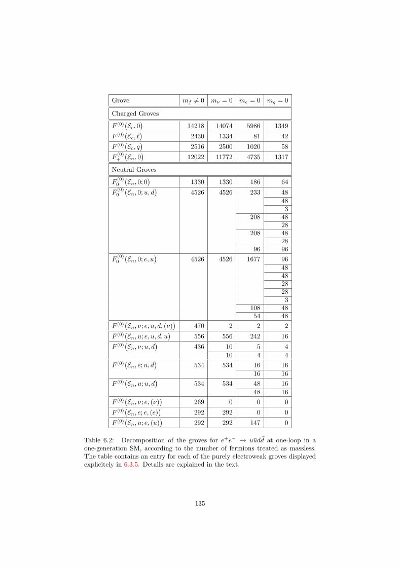
Grove mf 6= 0 mν = 0 me = 0 mq = 0

Charged Groves

F (0)(Ec, 0

)14218 14074 5986 1349

F (0)(Ec, `

)2430 1334 81 42

F (0)(Ec, q

)2516 2500 1020 58

F(0)+

(En, 0

)12022 11772 4735 1317

Neutral Groves

F(0)0

(En, 0; 0

)1330 1330 186 64

F(0)0

(En, 0;u, d

)4526 4526 233 48

483

208 4828

208 4828

96 96F

(0)0

(En, 0; e, u

)4526 4526 1677 96

484828283

108 4854 48

F (0)(En, ν; e, u, d, (ν)

)470 2 2 2

F (0)(En, u; e, u, d, u

)556 556 242 16

F (0)(En, ν;u, d

)436 10 5 4

10 4 4F (0)

(En, e;u, d

)534 534 16 16

16 16F (0)

(En, u;u, d

)534 534 48 16

48 16F (0)

(En, ν; e, (ν)

)269 0 0 0

F (0)(En, e; e, (e)

)292 292 0 0

F (0)(En, u; e, (u)

)292 292 147 0

Table 6.2: Decomposition of the groves for e+e− → uudd at one-loop in aone-generation SM, according to the number of fermions treated as massless.The table contains an entry for each of the purely electroweak groves displayedexplicitely in 6.3.5. Details are explained in the text.

135

—7—Summary

The experimental accuracy of planned high energy physics experiments at fu-ture particle colliders requires equally accurate theoretical predictions for themeasured observables like cross sections, branching ratios, decay widths etc. Inorder to achieve the required precision, radiative corrections have to be included.

Now, in the Standard model, scattering amplitudes and decay matrix ele-ments are usually computed from a perturbative expansion defined in terms ofFeynman diagrams. The inclusion of radiative corrections to these quantitiesimplies that Feynman diagrams with loops have to be taken into account. Thisis a difficult problem, mainly for two reasons: On one hand, the number ofFeynman diagrams contributing to a particular Standard Model process growsvery rapidly with the number of loops and the number of external particles. Onthe other hand, the Standard Model being a gauge theory, care must be takennot to violate gauge invariance.

The resulting complexity of Standard Model calculations makes the use ofautomatization indispensable. However, even with the computing power of mod-ern computers the construction of fully automated tools remains a challengingtask. For numerical reasons, one would therefore like to subdivide the calcu-lation of the scattering amplitude into smaller pieces, which independently ofeach other give sensible, i. e. gauge invariant, results. It is therefore of interestwhether a partitioning of the full set of diagrams contributing to a scatteringamplitude or decay matrix element into separately gauge invariant pieces canbe found.

For the lowest order scattering amplitude, i. e. the set of tree level diagrams,an algorithm for the construction of minimal gauge invariant subsets has beendescribed in [4] and formally proven in [5]. The algorithm uses a set of graphicaloperations on Feynman diagrams, called gauge flips, to decompose the full setof Feynman diagrams into the minimal gauge invariant subsets.

In the present work, we have extended this algorithm to Feynman diagramswith loops. To this end, we have studied the Slavnov-Taylor-Identities of con-nected Green’s functions in a general gauge theory. We have shown how theSTI for the expansion of a connected Green’s function at n-loop order followsfrom the STIs for the tree level vertices of the theory. We have then used thegained insight to show that the gauge flips of [4] can indeed be used to constructminimal gauge invariant subsets also for diagrams with loops.

We emphasize that, although diagrammatical proofs for the STIs in gaugetheories have been given before [26][27], they make statements only about thefull set of diagrams defining the expansion of the Green’s function under consid-

136

eration. Therefore, our proof of the STIs for subsets of the full set of Feynmandiagrams is original.

We have then used the formalism of gauge flips to derive rules for a clas-sifcation of the minimal gauge invariant subsets of general connected Green’sfunctions in the Standard Model. Using these rules, we have studied the minimalgauge invariant subsets of a specific Standard Model process. The theoreticalresults so obtained were then confirmed and further illustrated by reexaminingthe diagrams for this process by means of a computer program for the con-struction of the minimal gauge invariant subsets for Feynman diagrams withloops, which we have designed and implemented on the basis of the theoreticalconsiderations in this work.

The explicit results we obtained show that the decomposition of the full setof diagrams into minimal gauge invariant subsets leads to a moderate reductionof the combinatorial complexity.

137

—A—BRST Feynman Rules

In this appendix, we collect the Feynman rules for insertions of the operatorssϕ, where s is the generator of BRST transformations and ϕ a generic field ofthe gauge theory. sϕ is split into an inhomogeneous part and a homogeneouspart according to (2.26):

sϕ = %ϕ[c] + ca∆aϕ . (A.1)

The inhomogeneous part, %ϕ[c] is, in fact, nonzero only for gauge bosons orGoldstone bosons.

The Feynman rules for the homogeneous part can be read off from the BRSTtransformation laws (2.18) and (2.60). We shall refer to them as BRST vertices.

In order to define the Feynman rules for the inhomogeneous parts, we mustcarefully distinguish between connected Green’s functions and 1PI Green’s func-tions, because identical symbols are used for different expressions. We havepointed out in section 2.5, why this is indeed useful. Anyway, we shall empha-size the distinction clearly below.

A.1 Unbroken Gauge Theories

We use the conventions of section 2.1 to denote fields and generators of thegauge group. The fields are represented with the following line styles:

W aµ → (A.2)

Φj → (A.3)ψj , ψj

→ ψ ψ (A.4)

ca, ca → c c (A.5)

A.1.1 BRST Vertices

a, µ

b

c, ν

= −gfabcδνµ (A.6)

a

b

c

= −gfabc (A.7)

138

j

k

a

= igtajk (A.8)

j

k

a

= −igtakj (A.9)

j

a

k

= −gXajk (A.10)

A.1.2 Inhomogeneous Parts

First, we list the Feynman rules for connected Green’s functions, which aredistinguished by the dot at the end of the line. Note that the momentum isdirected from left to right.

p

µ= −ipµ

p(A.11)

p

µ= −1

ξipν

p

ν µ(A.12)

Now, we specify the Feynman rules for 1PI Green’s functions. Again, themomentum points from left to right.

p

µ=

1ξipµ (A.13)

p

µ= −ipµ (A.14)

A.2 Spontaneously Broken Gauge Theories

For spontaneously broken gauge theories, we use the conventions of section 2.2.2.In particular, to denote the generators of the gauge group, we use the lettersa, b, c for arbitrary generators, α, β, γ for broken generators, and q, r, s forunbroken generators.

The scalar multiplet Φ is decomposed into Goldstone bosons φ and Higgsbosons H according to:

Φ =(

φv +H

)(A.15)

In this basis, the generators Xa in the scalar sector are parametrized as follows:

Xa =(

ta ua

−(ua)T T a

)(A.16)

Of course, uq = 0 for unbroken generators.Gauge bosons and Goldstone bosons are combined into a five-dimensional

gauge field as in (2.64):Aa

r =(W a

µ , φa)

(A.17)

139

In Feynman rules, gauge bosons and Goldstone bosons will then be distinguishedby the five-dimensional index, which is a Lorentz index (µ or ν) for gauge bosons,and 4 for Goldstone bosons.

The following line styles are used to represent the fields of a spontaneouslybroken gauge theory:

Aar → (A.18)

Hj → (A.19)ψj , ψj

→ ψ ψ (A.20)

ca, ca → c c (A.21)

A.2.1 BRST Vertices

Note that, for all particles but scalars, the BRST Feynman rules for the homo-geneous parts are identical to the rules in an unbroken theory. Therefore we listonly the rules for scalars:

α, 4

β

γ, 4

= −gtβαγ (A.22)

α, 4q

β, 4

= −gtβαγ (A.23)

α, 4

β

j

= −guβαj (A.24)

j

α

β, 4

= guαjβ (A.25)

j

α

k

= −gTαjk (A.26)

A.2.2 Inhomogeneous Parts

To define the Feynman rules for the inhomogeneous parts in the BRST trans-formation laws of gauge bosons and Goldstone bosons, we make use of the five-dimensional contraction operators Θ(p) and ¯Θ(p), defined in (2.93) and (2.94):

Θr(p) =(−ipµ,−M

)(A.27)

Θr(p) =(

1ξipµ,M

). (A.28)

These formulae can be taken over for massless gauge bosons by setting M = 0.

140

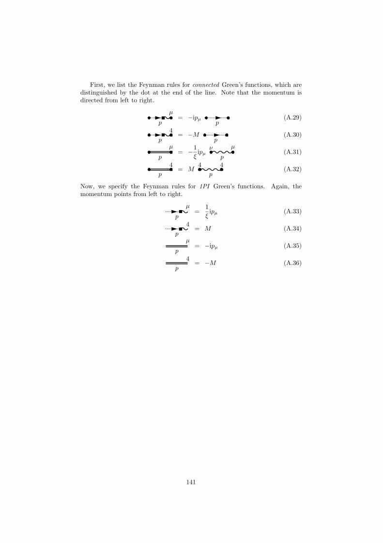
First, we list the Feynman rules for connected Green’s functions, which aredistinguished by the dot at the end of the line. Note that the momentum isdirected from left to right.

p

µ= −ipµ

p(A.29)

p

4= −M

p(A.30)

p

µ= −1

ξipµ

p

ν µ(A.31)

p

4= M

p

4 4(A.32)

Now, we specify the Feynman rules for 1PI Green’s functions. Again, themomentum points from left to right.

p

µ=

1ξipµ (A.33)

p

4= M (A.34)

p

µ= −ipµ (A.35)

p

4= −M (A.36)

141

—B—Tree Level STIs

In this appendix we collect all tree level STIs used in the proof of the STI forconnected Green’s functions in chapter 4.

B.1 Propagator and Inverse Propagator STIs

= − (B.1)

= − . (B.2)

Note in particular the minus sign.

B.2 Vertex STIs

B.2.1 Cubic Vertices

In the STIs for cubic vertices, the lines with a cross at the end denote a treelevel inverse propagator. (Cf. (3.6))

0 = + + + + .

(B.3)

0 = − + . (B.4)

For use inside larger diagrams, the STIs (B.3) and (B.4) are often inconvenientdue to the occurrence of the inverse propagators. Therefore, we list separatelythe STIs obtained from (B.3) and (B.4) by multiplying with three propagators.Note the sign changes.

= + + + (B.5)

142

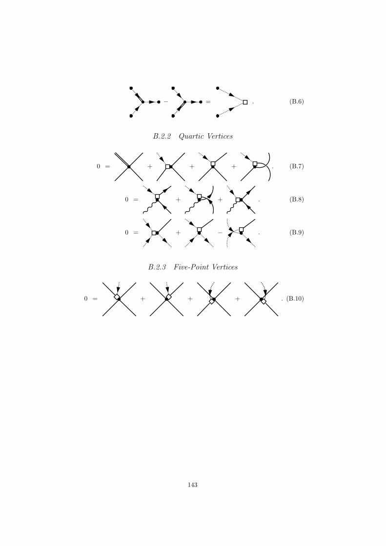
− = . (B.6)

B.2.2 Quartic Vertices

0 = + + + . (B.7)

0 = + + . (B.8)

0 = + − . (B.9)

B.2.3 Five-Point Vertices

0 = + + + . (B.10)

143

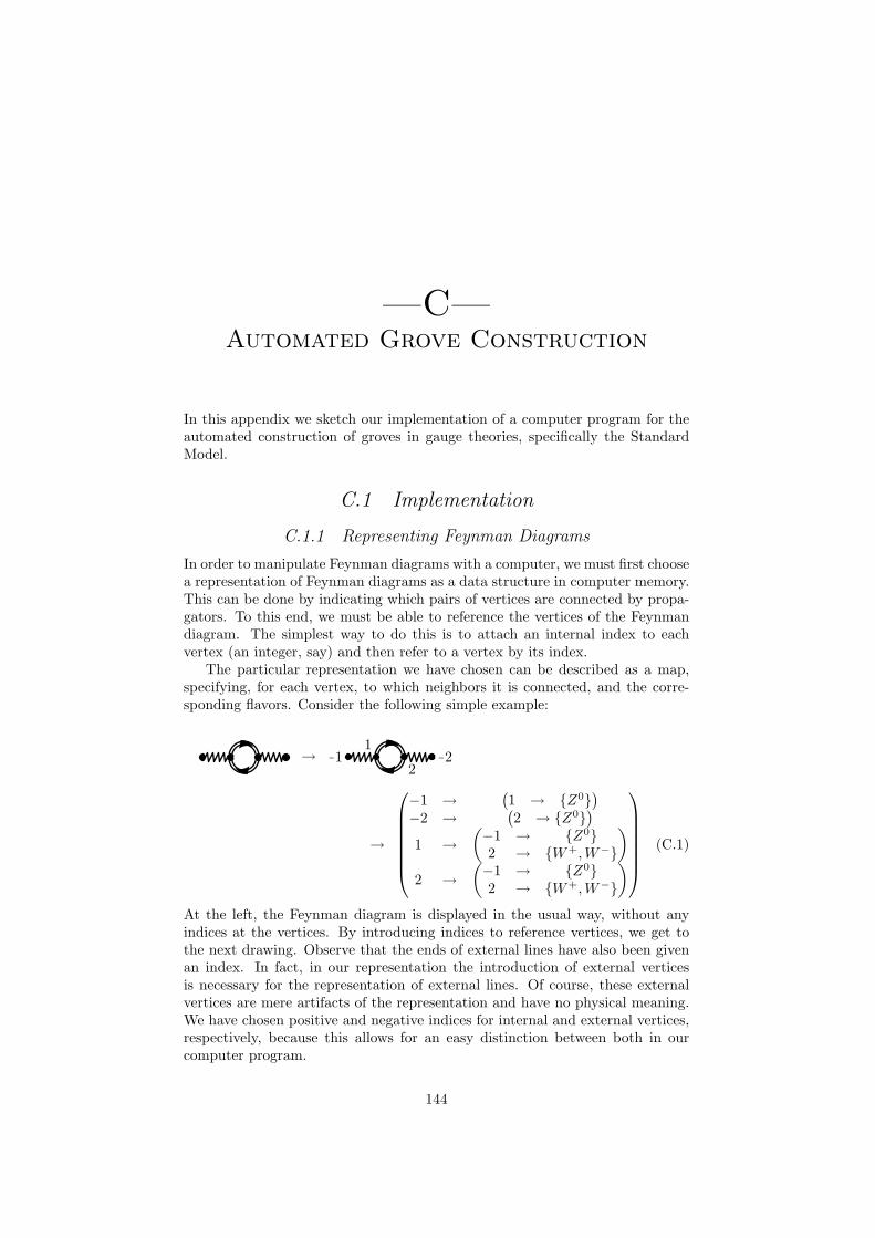
—C—Automated Grove Construction

In this appendix we sketch our implementation of a computer program for theautomated construction of groves in gauge theories, specifically the StandardModel.

C.1 Implementation

C.1.1 Representing Feynman Diagrams

In order to manipulate Feynman diagrams with a computer, we must first choosea representation of Feynman diagrams as a data structure in computer memory.This can be done by indicating which pairs of vertices are connected by propa-gators. To this end, we must be able to reference the vertices of the Feynmandiagram. The simplest way to do this is to attach an internal index to eachvertex (an integer, say) and then refer to a vertex by its index.

The particular representation we have chosen can be described as a map,specifying, for each vertex, to which neighbors it is connected, and the corre-sponding flavors. Consider the following simple example:

→ 91 921

2

→

−1 →

(1 → Z0

)−2 →

(2 → Z0

)1 →

(−1 → Z02 → W+,W−

)2 →

(−1 → Z02 → W+,W−

)

(C.1)

At the left, the Feynman diagram is displayed in the usual way, without anyindices at the vertices. By introducing indices to reference vertices, we get tothe next drawing. Observe that the ends of external lines have also been givenan index. In fact, in our representation the introduction of external verticesis necessary for the representation of external lines. Of course, these externalvertices are mere artifacts of the representation and have no physical meaning.We have chosen positive and negative indices for internal and external vertices,respectively, because this allows for an easy distinction between both in ourcomputer program.

144

The indexed Feynman diagram is easily translated into the displayed map.For instance, one should read the first entry as stating that “vertex 91 is con-nected to vertex 1 by a Z0-line”. Observe that the notation for the map is stillan abstract representation. There may be many different ways to implementsuch a map as a data structure. However, it turns out that, in order to dealwith comparisons efficiently (cf. the next section), the chosen data structureshould satisfy the constraint that identical maps correspond to identical datastructures.

C.1.2 Comparing Feynman Diagrams

The algorithm for the construction of groves instructs us to repeatedly addall gauge flipped diagrams to a given set of diagrams, starting from a singlediagram, until no more new diagrams are created. In order to implement thisalgorithm, we have to be able to test the representations of Feynman diagramsin computer memory for equality, or else we will not be able to assert whetheror not a diagram has already been produced.

We have already argued that our representation of Feynman diagrams withloops introduces indices to identify the vertices of the diagram. However, theseindices are unrelated to the physical meaning of Feynman diagrams. Therefore,two representations of Feynman diagrams that differ only by a permutation ofthe vertex indices actually denote the same Feynman diagram. On the otherhand, different permutations of indices will usually lead to different data struc-tures (unless the permutation corresponds to an automorphism of the Feynmandiagram). This means that we cannot naively compare representations, i. e. datastructures in computer memory, in order to test two Feynman diagrams forequality.

We can, however, compare representations if we find a prescription to pro-duce a unique indexation for every possible Feynman diagram. In graph theory,this strategy is formalized by considering permutations of indices as an equiva-lence relation on the set of representations of Feynman diagrams. A Feynmandiagram corresponds then actually to an equivalence class of representations. Aunique prescription to pick a representative from an equivalence class is said tobe a canonical label. Accordingly, the corresponding representative is called acanonical representative. Given a canonical label, two Feynman diagrams can becompared by comparing the data structures of their canonical representatives.

We have based our canonical label algorithm on the algorithm nauty,[28]by adapting it to the peculiarities of Feynman diagrams with loops. Due tothe nature of the nauty algorithm, we are able to produce not only canonicalrepresentatives of Feynman diagrams, where external lines are assumed to carrydistinct momenta, but also topologies of Feynman diagrams, by ignoring themomenta of some or all external lines. Recall that, for forests with externalfermions, the groves can be characterized by permutations of identical fermions.Our canonical label algorithm allows for a simple way to produce just one of allpossible permutations.

C.1.3 Constructing Groves

Given an implementation of flips for canonically labeled Feynman diagrams, theconstruction of groves is performed precisely as described in the main part of

145

this work, by partitioning the forest.At present, we use an external program, qgraf,[29] for the production of the

forest. The groves can then be constructed by a simple depth-first-search.On the other hand, since the unflavored forest is connected according to the

results of chapter 5, it is also possible to construct the groves incrementally,starting from a single diagram. In particular, once the grove correspondingto the first diagram has been completed, we try to obtain a new diagram byperforming unflavored non-gauge flips. If we find one, it can be used to constructa new grove, and we can repeat the procedure. If no more new diagram is found,the forest must be complete.

This strategy is, however, not very well suited for theories with many differ-ent fermion flavors, like the SM. The reason is that, in order for the forest to beconnected, we must ignore the fermion flavors completely. But this will generallylead to the production of redundant diagrams, because the unflavored diagramsgenerated may not be compatible with the flavors of the actual external state.

C.2 Usage

We have actually written two implementations of the algorithm for grove con-struction: The first one, mangroves, deals with general gauge theories, whilethe second one, smgroves, is tailored to the special properties of the StandardModel. It is the latter implementation that we have used to produce the resultsof section 6.3.7 and that we shall describe here.

The program smgroves is run from the command line. To illustrate thepossible options, we display the output of the command smgroves -help:1

Usage: smgroves [options] -l #loops flavor_1 ... flavor_n-sm:no_fermions SM without fermions.-sm:one_dublet SM with a single quark dublet.-sm:one_generation SM with one lepton and one quark.-sm:massive_neutrinos SM with all fermions massive.-sm:massless_neutrinos SM with massless neutrinos.-sm:massless_leptons SM with massless leptons.-sm:massless_fermions SM with massless fermions.-sm:with_ghosts Include ghost diagrams.-sm:with_QCD Include QCD contributions.-qcd n Select of order n in alpha_s.-onshell Select amputated diagrams.-onepi Select 1PI diagrams.-notadpoles Omit diagrams with tadpoles.-topl Produce topologies, not diagrams.-help Display this list of options--help Display this list of options

As can be seen, smgroves must be given the number of loops and the set ofexternal flavors. Further options can be used to control the particle and couplingcontent of the SM.

A typical invocation of smgroves is given by:1There are actually more options, most of them for controlling the output of smgroves,

which are not listed here.

146

smgroves \-sm:one_generation -sm:massive_fermions \-sm:with_QCD -qcd 2 -l 1 ep em u ubar d dbar

In fact, the groves of the O(α1s) contributions to the mf 6= 0 case in the example

of section 6.3.7 have been generated with precisely this command. The outputof smgroves for this run has been used to produce the O(α1

s) entry in table 6.1.In addition to the program smgroves, we have written a helper program

smanalyze to determine the inclusion of groves for different choices of masslessfermions. This program has been used to produce the numbers in table 6.2.

147

Bibliography

[1] L. Dixon, in QCD and beyond, edited by D. E. Soper (World Scientific,Singapore, 1996), p. 539, hep-ph/9601359.

[2] M. Moretti, T. Ohl, and J. Reuter, O’Mega: An optimizing matrix ele-ment generator, Technical Report No. LC-TOOL-2001-040, DESY, in *2ndECFA/DESY Study 1998-2001* 1981-2009 (2001).

[3] F. Caravaglios and M. Moretti, Phys. Lett. B358, 332 (1995).

[4] E. Boos and T. Ohl, Phys. Rev. Lett. 83, 480 (1999), hep-ph/9903357.

[5] C. Schwinn, Gauge Checks, Consistency of Approximation Schemes andNumerical Evaluation of Scattering Amplitudes, 2003, PhD thesis, TU-Darmstadt.

[6] D. Ondreka, Eichinvarianzklassen von Feynman-Diagrammen in einerEichtheorie mit Fermionen in irreduziblen SU(2)-Darstellungen, 2000,Diplomarbeit, TU-Darmstadt.

[7] P. A. M. Dirac, Lectures on Quantum Mechanics (Yeshiva University, NewYork, 1964).

[8] L. D. Faddeev and V. N. Popov, Phys. Lett. 25B, 29 (1967).

[9] C. Becchi, A. Rouet, and R. Stora, Ann. Phys. 98, 287 (1976).

[10] I. V. Tyutin, Lebedev Institute preprint N39, 1975.

[11] N. Nakanishi, Prog. Theor. Phys. 35, (1966).

[12] B. E. Lautrup, Mat. Phys. Medd. Kon. Dan. Vid.-Sel. Medd. 35, (1967).

[13] T. Kugo and I. Ojima, Prog. Theor. Phys. Suppl. 66, 1 (1979).

[14] O. Piguet, Algebraic Renormalization: Perturbative Renormalization, Sym-metries and Anomalies (Springer, Berlin, 1995).

[15] A. A. Slavnov, Theo. Math. Phys. 10, 99 (1972).

[16] J. C. Taylor, Nucl. Phys. B33, 436 (1971).

[17] B. W. Lee and J. Zinn-Justin, Phys. Rev. D5, 3121 (1972).

[18] B. W. Lee, in Methods in Field Theory, edited by R. Balian and J. Zinn-Justin (North-Holland/World-Scientific, Amsterdam, 1976), p. 77.

149

[19] J. Goldstone, Nouvo Cim. 19, 154 (1961).

[20] J. Goldstone, A. Salam, and S. Weinberg, Phys. Rev. 127, 965 (1962).

[21] G. ’t Hooft, Nucl. Phys. B35, 167 (1971).

[22] O. Piguet and K. Sibold, Nucl. Phys. B253, 517 (1985); E. Kraus and K.Sibold, Nucl. Phys. B (Proc. Suppl.) 37B, 120 (1994); O. M. D. Cima,D. H. T. Franco, and O. Piguet, Nucl. Phys. B551, 813 (1999).

[23] C. Schwinn, Forests and Groves: From Trees To Loops, work in preparation.

[24] M. E. Peskin and D. V. Schroeder, An Introduction To Quantum FieldTheory (Addison-Wesley, Reading, USA, 1995), p. 842.

[25] G. ’t Hooft and M. Veltman, Nucl. Phys. B44, 189 (1972).

[26] G. ’t Hooft, Nucl. Phys. B33, 173 (1971).

[27] G. ’t Hooft and M. Veltman, Nucl. Phys. B50, 318 (1972).

[28] B. D. McKay, Congressus Numerantium 30, 45 (1981).

[29] P. Nogueira, J. Comp. Phys. 105, 279 (1993).

150

Danksagung

Ich danke Herrn Prof. Manakos fur die Aufnahme in seine Arbeitsgruppe unddafur, dass er es mir ermoglicht hat, diese Arbeit anzufertigen. Mein besondererDank gilt Herrn Dr. Thorsten Ohl, der mein Interesse am Thema der Arbeitgeweckt hat, fur seine guten Ratschlage, seine Geduld und sein LATEX-PaketFeynMF. Großen Dank schulde ich auch meinem Kollegen Dr. Christian Schwinnfur die vielen fruchtbaren und geistreichen Diskussionen uber Eichtheorien undfur wertvolle Hinweise auf die richtige Literatur.

Danken mochte ich auch den Mitgliedern der Arbeitsgruppen von HerrnProf. Wambach und Herrn Prof. Roth fur die gute Atmosphare im vierten Stock-werk und fur die Anschaffung der Kaffeemaschine. Bei Dominik Nickel, Dr. AxelMaas und Dr. Bernd-Jochen ”BJ“ Schaefer bedanke ich mich fur einige hilfrei-che Diskussionen uber Physik. Herzlichen Dank auch an Verena Werth, MarkusHild, Mathias Wagner und Dr. Thomas Roth fur die taglichen Espresso- undCappucino-Pausen. Bei Mathias Wagner und Thomas Roth mochte ich michinsbesondere auch fur ihre Hilfe bei Computerproblemen jeglicher Art bedan-ken.

Nicht zuletzt mochte ich auch meiner Familie danken, am meisten und in-nigsten meiner Frau Felizitas fur die Unterstutzung, die sie mir hat zuteil werdenlassen, und fur die Geduld, mit der sie meine langen Arbeitszeiten in den heißenPhasen der Fertigstellung dieser Arbeit ertragen hat. Danken mochte ich auchmeinen Kindern, die mich oft genug vermisst haben, fur ihr Verstandnis. De-nen, die noch zu klein sind, um Verstandnis zu haben, danke ich dafur, dass siemich, wenn es darauf ankam, doch wieder haben schlafen lassen. Fur die Betreu-ung der Kinder mochte ich mich auch bei meinen Eltern und Schwiegerelternbedanken.

Diese Arbeit wurde in Teilen vom Bundesministerium fur Bildung und For-schung, Deutschland, unterstutzt. (O5HT1RDA/6)

151

Lebenslauf

David OndrekaScheffelstraße 863071 Offenbach

Personliche Daten

Geburt: 27. 8. 1973 in Hanau

Eltern: Werner Ondreka (Hausmann) und Eva-Maria Ondreka (Bibliotheka-rin)

Familienstand: verheiratet, funf Kinder

Staatsangehorigkeit: deutsch

Ausbildung

1980-1984 Grundschule Buchhugel Offenbach

1984-1986 Bachschule Offenbach

1986-1993 Leibniz-Gymnasium Offenbach

1993 Abitur mit der Durchschnittsnote 1.0

1993-1994 Wehrdienst bei der Bundesmarine in Eckernforde

1994-2000 Physikstudium an der TU Darmstadt

1996 Vordiplom mit der Note ”sehr gut“

seit 1998 Betreuung von Ubungsgruppen im Fach Theoretische Physik

153

Juni 2000 Diplomprufung. Diplomarbeit mit dem Titel ”Eichinvarianzklassenvon Feynman-Diagrammen in einer Eichtheorie mit Fermionen in irredu-ziblen SU(2)-Darstellungen“ in der Arbeitsgruppe von Prof. Manakos ander TU Darmstadt

Juli 2000 Beginn der Doktorarbeit auf dem Gebiet der theoretischen Elementar-teilchenphysik in der Arbeitsgruppe von Prof. Manakos an der TU Darm-stadt

September 2001 Teilnahme an der Herbstschule fur Hochenergiephysik inMaria Laach

154

Eidesstattliche Erklarung

Hiermit erklare ich an Eides statt, dass ich die vorliegende Arbeit selbstandigund nur mit den angegebenen Hilfsmitteln angefertigt habe. Ich habe vorherkeinen weiteren Promotionsversuch unternommen.

Darmstadt, 11. April 2005

David Ondreka

155

Construction of Minimal Gauge Invariant Subsets of Feynman ... · Construction of Minimal Gauge...

Documents

Transcript of Construction of Minimal Gauge Invariant Subsets of Feynman ... · Construction of Minimal Gauge...