CONSTRUCTION OF LARGE-PERIOD SYMPLECTIC MAPS BYINTERPOLATIVE METHODS ∗

Robert L. Warnock † and Yunhai Cai‡

SLAC National Accelerator Laboratory, Stanford University, Menlo Park, CA 94025, USAJames A. Ellison§

Dept. of Mathematics and Statistics, University of New Mexico, Albuquerque, NM 87131, USA

Abstract

The goal is to construct a symplectic evolution map fora large section of an accelerator, say a full turn of a largering or a long wiggler. We start with an accurate track-ing algorithm for single particles, which is allowed to beslightly non-symplectic. By tracking many particles fora distance S one acquires sufficient data to construct themixed-variable generator of a symplectic map for evolu-tion over S, given in terms of interpolatory functions. Twoways to find the generator are considered: (i) Find its gra-dient from tracking data, then the generator itself as a lineintegral. (ii) Compute the action integral on many orbits. Atest of method (i) has been made in a difficult example: afull turn map for an electron ring with strong nonlinearitynear the dynamic aperture. The method succeeds at fairlylarge amplitudes, but there are technical difficulties nearthe dynamic aperture due to oddly shaped interpolation do-mains. For a generally applicable algorithm we proposemethod (ii), realized with meshless interpolation methods.

1. INTRODUCTION

The method of differential algebra, giving automatic dif-ferentiation of functions defined by complex algorithms,allows the construction of the truncated Taylor series of amap defined by a tracking code. After this method was im-plemented by Martin Berz [1], the option of producing aTaylor map eventually became a feature of several trackingcodes. The Taylor map is not symplectic, but some codesuse the Taylor coefficients to produce the mixed-variablegenerator of a symplectic map, itself represented as a trun-cated power series [2]. Another way is to use the Taylorcoefficients to form the symplectic “jolt factorization” ofIrwin, Abell, and Dragt [3]. The Taylor map, symplectifiedor not, is good at small phase space amplitudes, but has arange of usefulness at larger amplitudes that varies with thetype of accelerator lattice considered. It appears to be fairlyuseful for hadron rings, but can fail badly for electron ringswith stronger nonlinearity near the dynamic aperture. Inthis paper we choose such a lattice for a demanding test ofmapping methods.

∗Work supported in part by U.S. Department of Energy contracts DE-AC02-76SF00515 and DE-FG-99ER41104.

† warnock@slac.stanford.edu; also affiliated with LBNL and UNM.‡ yunhai@slac.stanford.edu§ ellison@math.unm.edu

−0.05 0 0.05

−0.01

−0.005

0

0.005

0.01

q

p

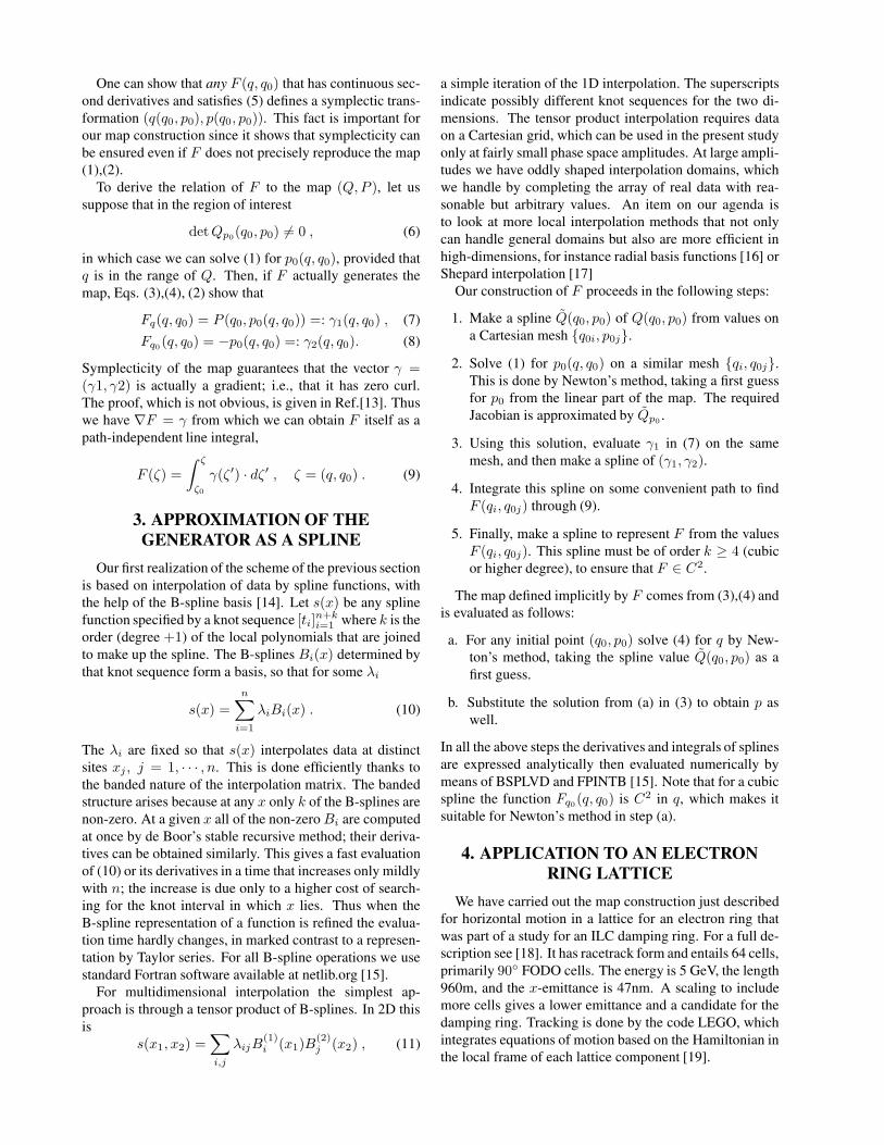
Figure 1: Phase plot from element-by-element tracking,1000 turns, νx = 16.23.

For our example the Taylor map fails at large amplitudes.For a striking illustration we choose a tune νx = 16.23.Element-by-element tracking gives the plot of Fig.1 on aPoincare section at a fixed position in the ring; p is dimen-sionless and q is in meters. The corresponding plot fromiteration of the 10th order Taylor map is shown in Fig.2.The prominent 9th order island chain is only vaguely vis-ible, and there is spurious stochasticity. The result is notimproved by going to 13th order. The symplectified Taylormap [2] shows islands and gets rid of the stochasticity, butthe shape of phase contours is all wrong. Changing to abetter tune of νx = 15.81, for which the lattice has a muchlarger dynamic aperture, we find that the Taylor map stillbreaks down at about the same amplitude.

One can easily see, however, that producing a more suc-cessful map when the Taylor series fails is not out of thequestion. A spline fit to one-turn tracking data on a gridof initial conditions gives a map which produces the plotof Fig.3 in 1000 iterations. To graphical accuracy it agreeswith the tracking map of Fig.1, but the symplectic condi-tion is badly violated at large amplitudes: the determinantof the map’s Jacobian differs from 1 at some points by asmuch as 0.004. Nevertheless it does not do badly over 105

iterations, as is seen in Fig.4. The main features of thephase plot persist correctly, but fuzziness appears near endsof the islands. By 106 turns there is a clear failure, withspurious damping, whereas phase curves including the is-lands are sharply defined in tracking for 106 turns. Thespline is a tensor product B-spline interpolating tracking

SLAC-PUB-13867

−0.05 0 0.05

−0.01

−0.005

0

0.005

0.01

q

p

Figure 2: Phase plot from 10th order Taylor map, 1000turns, νx = 16.23.

−0.05 0 0.05

−0.01

−0.005

0

0.005

0.01

q

p

Figure 3: Phase plot from Spline Map, 1000 turns, νx =16.23.

data on a 40 × 40 uniform mesh; the spline coefficientswere determined in 0.6 sec, and the time for 105 iterationswas 0.14 sec. Computation times are for a single 2.66 GHzprocessor.

This example supports our belief that interpolative meth-ods can produce maps that are both accurate and fast, evenin cases where power series are not useful. Actually, thepromise of interpolative map construction was evident longago, in the work of Refs.[4, 5, 6, 7]. That work resulted inthe generator of a fast symplectic map represented in po-lar coordinates in a hybrid Fourier-spline basis. It was ap-plied successfully to an early LHC lattice, but in a slightlyrestricted region of phase space owing to a coordinate sin-gularity arising from the polar coordinates. In work go-ing back to 1984, G. Wustefeld and collaborators have ap-plied generating functions to maps for complicated mag-netic fields, sometimes using interpolative methods [8].

In 1999 two of the authors proposed a method to findthe map generator in Cartesian coordinates, with splinesin all variables [9]. (Earlier, Berz had described a for-mally similar construction of the generator, but to be re-alized through power series rather than splines [10].) The

−0.05 0 0.05

−0.01

−0.005

0

0.005

0.01

q

p

Figure 4: Phase plot from Spline Map, 105 turns, νx =16.23.

present paper gives the first numerical implementation ofthe scheme of Ref.[9]. Another idea, which came to lightwhen one of the authors was preparing an article on theHamilton-Jacobi equation [11], is to compute the genera-tor directly as Hamilton’s Principal Function, which is theintegral of the Lagrangian regarded as a function of initialand final spatial coordinates.

2. RELATION OF THE GENERATOR TOTHE TRACKING MAP

We denote the map defined through an element-by-element tracking code as follows:

q = Q(q0, p0) , (1)

p = P (q0, p0) , (2)

where z = (q, p) = (z1, · · · , z2n) and z0 = (q0, p0) arefinal and initial phase space points for a system with n de-grees of freedom. The map can refer to an arbitrary periodin a circular or linear machine, but in the present applica-tion it is for one turn of a circular machine. In the the-ory of canonical transformations [11] the map is expressedimplicitly in terms of a generating function or generator,which we take to be a “Type 1” generator of the formF (q, q0). The implicit map is defined by the equations

p = Fq(q, q0) , (3)

p0 = −Fq0(q, q0) , (4)

where subscripts denote partial derivatives: Fq =(∂F/∂q1, · · · , ∂F/∂qn). We suppose that for q and q0 inthe region of interest, the n×n Hessian matrix Fqq0 is non-singular:

detFqq0 (q, q0) �= 0 . (5)

Then one can solve (4) for q = q(q0, p0) (at least locally)and substitute the result in (3) to obtain also p(q0, p0) =Fq(q(q0, p0), q0) [12]. We wish to determine F so that thefunctions q(q0, p0), p(q0, p0) can be identified with the mapcomponents Q(q0, p0), P (q0, p0).

One can show that any F (q, q0) that has continuous sec-ond derivatives and satisfies (5) defines a symplectic trans-formation (q(q0, p0), p(q0, p0)). This fact is important forour map construction since it shows that symplecticity canbe ensured even if F does not precisely reproduce the map(1),(2).

To derive the relation of F to the map (Q, P ), let ussuppose that in the region of interest

detQp0(q0, p0) �= 0 , (6)

in which case we can solve (1) for p0(q, q0), provided thatq is in the range of Q. Then, if F actually generates themap, Eqs. (3),(4), (2) show that

Fq(q, q0) = P (q0, p0(q, q0)) =: γ1(q, q0) , (7)

Fq0 (q, q0) = −p0(q, q0) =: γ2(q, q0). (8)

Symplecticity of the map guarantees that the vector γ =(γ1, γ2) is actually a gradient; i.e., that it has zero curl.The proof, which is not obvious, is given in Ref.[13]. Thuswe have ∇F = γ from which we can obtain F itself as apath-independent line integral,

F (ζ) =∫ ζ

ζ0

γ(ζ′) · dζ′ , ζ = (q, q0) . (9)

3. APPROXIMATION OF THEGENERATOR AS A SPLINE

Our first realization of the scheme of the previous sectionis based on interpolation of data by spline functions, withthe help of the B-spline basis [14]. Let s(x) be any splinefunction specified by a knot sequence [ti]n+k

i=1 where k is theorder (degree +1) of the local polynomials that are joinedto make up the spline. The B-splines Bi(x) determined bythat knot sequence form a basis, so that for some λi

s(x) =n∑

i=1

λiBi(x) . (10)

The λi are fixed so that s(x) interpolates data at distinctsites xj , j = 1, · · · , n. This is done efficiently thanks tothe banded nature of the interpolation matrix. The bandedstructure arises because at any x only k of the B-splines arenon-zero. At a given x all of the non-zero Bi are computedat once by de Boor’s stable recursive method; their deriva-tives can be obtained similarly. This gives a fast evaluationof (10) or its derivatives in a time that increases only mildlywith n; the increase is due only to a higher cost of search-ing for the knot interval in which x lies. Thus when theB-spline representation of a function is refined the evalua-tion time hardly changes, in marked contrast to a represen-tation by Taylor series. For all B-spline operations we usestandard Fortran software available at netlib.org [15].

For multidimensional interpolation the simplest ap-proach is through a tensor product of B-splines. In 2D thisis

s(x1, x2) =∑i,j

λijB(1)i (x1)B

(2)j (x2) , (11)

a simple iteration of the 1D interpolation. The superscriptsindicate possibly different knot sequences for the two di-mensions. The tensor product interpolation requires dataon a Cartesian grid, which can be used in the present studyonly at fairly small phase space amplitudes. At large ampli-tudes we have oddly shaped interpolation domains, whichwe handle by completing the array of real data with rea-sonable but arbitrary values. An item on our agenda isto look at more local interpolation methods that not onlycan handle general domains but also are more efficient inhigh-dimensions, for instance radial basis functions [16] orShepard interpolation [17]

Our construction of F proceeds in the following steps:

1. Make a spline Q(q0, p0) of Q(q0, p0) from values ona Cartesian mesh {q0i, p0j}.

2. Solve (1) for p0(q, q0) on a similar mesh {qi, q0j}.This is done by Newton’s method, taking a first guessfor p0 from the linear part of the map. The requiredJacobian is approximated by Qp0 .

3. Using this solution, evaluate γ1 in (7) on the samemesh, and then make a spline of (γ1, γ2).

4. Integrate this spline on some convenient path to findF (qi, q0j) through (9).

5. Finally, make a spline to represent F from the valuesF (qi, q0j). This spline must be of order k ≥ 4 (cubicor higher degree), to ensure that F ∈ C2.

The map defined implicitly by F comes from (3),(4) andis evaluated as follows:

a. For any initial point (q0, p0) solve (4) for q by New-ton’s method, taking the spline value Q(q0, p0) as afirst guess.

b. Substitute the solution from (a) in (3) to obtain p aswell.

In all the above steps the derivatives and integrals of splinesare expressed analytically then evaluated numerically bymeans of BSPLVD and FPINTB [15]. Note that for a cubicspline the function Fq0(q, q0) is C2 in q, which makes itsuitable for Newton’s method in step (a).

4. APPLICATION TO AN ELECTRONRING LATTICE

We have carried out the map construction just describedfor horizontal motion in a lattice for an electron ring thatwas part of a study for an ILC damping ring. For a full de-scription see [18]. It has racetrack form and entails 64 cells,primarily 90◦ FODO cells. The energy is 5 GeV, the length960m, and the x-emittance is 47nm. A scaling to includemore cells gives a lower emittance and a candidate for thedamping ring. Tracking is done by the code LEGO, whichintegrates equations of motion based on the Hamiltonian inthe local frame of each lattice component [19].

−0.08 −0.06 −0.04 −0.02 0 0.02 0.04 0.06 0.08 0.1

−0.02

−0.015

−0.01

−0.005

0

0.005

0.01

0.015

0.02

q (m)

p

Figure 5: Phase plot from tracking, νx = 15.81.Dynamic aperture (2000 turns) just beyond outer curve.

The motion of this example becomes very nonlinear asthe dynamic aperture is approached. This makes it a chal-lenging example for map construction. A hadron machinesuch as the LHC has weaker sextupoles and weaker nonlin-earity out to the dynamic aperture, notwithstanding impor-tant effects of random higher order multipoles which con-tribute to long-term diffusion. On the basis of earlier work[5, 6, 7] we expect that the present algorithm will be use-ful for the LHC over a bigger range of amplitudes than itis in the present example. Nevertheless, the difficulties ofthis example have been very informative, and the lessonslearned will certainly be relevant to other cases.

We now choose a tune, νx = 15.81, for which theshort term dynamic aperture is large, near the orbit with(q0, p0) = (7cm, 0). There are no easily found resonancesexcept for an 11th order one very close to the dynamic aper-ture. A phase plot is shown in Fig.5.

We try to construct a map on a rectangular region |q0| ≤r1, |p0| ≤ r2, and expect that some sub-region will bemapped into itself by the constructed map. We thereforeseek to construct F (q, q0) in a square domain, |q|, |q0| ≤r1. For r1 = 2.5cm everything goes according to the planof the previous section. This is in accord with the mathe-matical analysis of Ref.[9] which showed that the schemeshould work at small amplitude. Passing to r1 = 4.5cm,we encounter a new situation. The solution for p0(q, q0)does not exist in one corner of the domain, as is seen inFig.(6). Let us call this triangular region B, for BermudaTriangle. The Newton iteration, which converges beauti-fully elsewhere, diverges in B in a mode such that iteratesget larger and larger. To generate the plot of successful so-lutions in Fig.6 the Newton iteration was declared a failurewhen iterates p

(n)0 got bigger than a small multiple of r2, or

when it failed to converge to desired accuracy within a setmaximum number of iterations. As expected, the bound-ary of B corresponds closely to the curve along which thecondition of Eq.(6) first fails.

In order to make a tensor product spline of γ(q, q0) inspite of the missing values, we have to fill in the array

−0.05 0 0.05−0.05

−0.04

−0.03

−0.02

−0.01

0

0.01

0.02

0.03

0.04

0.05

q (m)

q0 (

m)

Figure 6: Points at which p0(q, q0) exists, in blue. Thecurves represent values of (q, q0) on the orbits of Fig.7.The path of integration for Eq.(9) is shown in red.

−0.05 0 0.05

−0.01

−0.005

0

0.005

0.01

q

p

Figure 7: Symplectic map from generator, 107 turns. Itera-tion time 20-25 sec. for 107 turns, per orbit.

in some reasonable manner. We choose to put in valuesclose to those on the boundary of B, line-by-line in the q-direction. Of course, the path in the line integral must avoidthe region B. We choose the path shown in Fig.6.

This procedure with a 50 × 50 mesh leads to a symplec-tic map that gives the phase plot of Fig.7, where each orbitis followed for 107 turns in 20-25 seconds. We have alsofollowed the outer orbit for 109 turns, finding no changeto graphical accuracy from the result of 107 turns. Map-ping time per turn is 20-200 times faster than the under-lying tracking code (depending on the tracking integratorchosen), but this is not a fair comparison since our trackingcode is not optimal for 2D tracking; it routinely computesthe time of flight which is not needed in 2D. Nevertheless,the timing suggests a good outlook for speed in higher di-mensions. The Newton iteration to solve (4) converged tomachine precision in two or three steps.

The plot of Fig.7 is graphically indistinguishable fromthe corresponding plot from tracking over 105 turns. Thequantitative agreement is not spectacular, however. At the

−0.08 −0.06 −0.04 −0.02 0 0.02 0.04 0.06 0.08 0.1−0.08

−0.06

−0.04

−0.02

0

0.02

0.04

0.06

0.08

0.1

q

q0

Figure 8: Two orbits in (q, q0) plane close to the boundaryof the region in which F (q, q0) exists. The dotted pointsare the same as those of Fig.6.

0.025 0.03 0.035 0.04 0.045 0.05 0.0550.055

0.06

0.065

0.07

0.075

0.08

0.085

0.09

q

q0

Figure 9: An enlargement of the top of Fig.8 showing in-tersecting orbits in (q, q0) plane.

one turn level we have agreement to 5 digits at small am-plitudes, declining to 4 digits at the outermost curve. Asthe map is iterated a lot of phase error quickly builds up,even though the iterates adhere to a clearly defined invari-ant curve. This is in accord with much earlier experiencein approximating maps. For a quantitative test in spite ofphase error one has to make an accurate representation ofan invariant curve from tracking, then see how well the mapfollows it; this can be done with the method of [20].

When we try to go beyond the outermost curve of Fig.7,the method abruptly breaks down. The reason can be un-derstood by using the tracking code to plot orbits in the(q, q0) coordinates for increasingly large amplitudes. Atsome point two curves for neighboring initial conditionscross, as is seen in the upper right corner of Fig.8. Thereare two crossings, as seen in the enlargement in Fig.9. Afterthis happens, the pair (q, q0) does not determine a uniqueorbit, hence p0(q, q0) is not a single-valued function andthe construction of F (q, q0) must fail. The curve withsmaller initial condition (q0 = 0.0604m, p0 = 0) roughly

defines the boundary of existence of F . As seen in Fig.8,the divergence of the Newton method defines part of theboundary quite accurately.

We should be able with sufficient care to construct thegenerator in its full region of existence. The reason thatour attempted construction failed abruptly with increasingamplitude is seen by comparing Fig.6 and Fig.8, both ofwhich show the points at which p0(q, q0) was determinedby Newton’s method. The orbits of higher amplitude thatwe seek go into the cusp-like region in the upper right cor-ner of Fig.8, but the path of integration used in the code canreach such points only by penetrating the boundary of theallowed region, thus giving nonsensical F . This could beavoided by a better choice of path, but that would be dif-ficult if not impossible to generalize to higher dimensions.Even with a better path, we have to face the problem of in-terpolation, which becomes increasingly awkward for thetensor product spline.

One might ask whether a generator F2(q, p0) exists whenF (q, q0) = F1(q, q0) does not. Plotting the same two or-bits of Fig.8 in (q, p0) coordinates, we find again two inter-sections but at negative q ≈ −.0605,−.025, rather than thepositive q ≈ .0375, .0475 of the intersections in (q, q0) co-ordinates. Thus when (q, q0) fails to specify an orbit (q, p0)succeeds, and vice versa. Each of the generators fails to ex-ist at some points on each of the two orbits. The symplec-tic condition in 2D phase space is Qq0Pp0 − Qp0Pq0 = 1which shows that Qp0 and Qq0 cannot vanish simultane-ously, hence either F1 or F2 must exist locally. A theoremin [21] generalizes this statement to higher dimensions.

5. GENERATOR CONSTRUCTION BYACTION INTEGRAL

We have shown one way to construct the generator,through a partial map inversion to give p0(q, q0) anda line integral. Another method goes back to Hamil-ton’s original work of 1830-1832 [11]. He obtainedthe generator through the integral of the Lagrangian.Namely,

S(q0, p0, t) =∫ t

0

[p(τ, z0) · q(τ, z0) − H(z(τ, z0), τ)

]dτ ,

(12)

where H is the Hamiltonian and the second argument of theorbit z(τ, z0) indicates its initial condition, z0 = (q0, p0).The time-like variable t would normally be path length s inaccelerator physics. Hamilton’s essential idea was to regardthe action as a function of (q, q0) rather than (q0, p0). Thenthe generator, which is a solution of the Hamilton-Jacobiequation called Hamilton’s Principal Function, is

F (q, q0, t) = S(q0, p0(q, q0, t), t) . (13)

This is identical to the function of the previous sectionswhen t = T is the period of the map.

The advantage of this formula for a practical construc-tion is that it avoids the line integral (9), which could bealmost impossible to deal with in higher dimensions withexcluded regions. A disadvantage is that the tracking codemust be augmented to calculate the action integral in thecourse of tracking. Fortunately, LEGO is able to furnishthe Hamiltonian needed in the integrand.

6. LOCAL INTERPOLATION AND THEUSE OF SCATTERED DATA

Tensor product splines may be adequate in many prob-lems but in general we need a more local sort of interpola-tion or approximation that can be used in non-rectangulardomains. One possibility is a generalized Shepard method[17] based on the formula

F (ζ) =∑

i

Pi(ζ)wi(ζ)∑j wj(ζ)

,

wi(ζ) = c(ζ − ζi)‖ζ − ζi‖−n , (14)

where n is a positive integer such as 4 or 6. Here Pi(ζ) is apolynomial that interpolates or approximates values of F atζi and a few nearby sites. The factor c(ζ − ζi) is a smoothcutoff that restricts the sum at any evaluation. For ζ closeto ζi this behaves like Pi(ζ) with small corrections fromother terms in the sum. The formula is globally smooth,with the degree of smoothness controlled by that of c.

This formula works when the sites ζi lie on a mesh oreven when they are scattered. In the latter case one wouldnormally use a least squares fit to determine the coefficientsof Pi, rather than strict interpolation, since the interpola-tion matrix could be nearly singular for some dispositionsof sites. Interpolation could be done by replacing the poly-nomial by a radial basis function [16].

As suggested by Fasshauer (private communication) itmay be advantageous to use scattered sites from a quasi-random (low discrepancy) sequence. This might enjoy theadvantage that quasi - Monte Carlo quadrature has overmesh based quadrature in high dimensions [22]. Such ascheme was tried in Ref.[23], in connection with solutionof a Vlasov equation. In 2D it was possible to reduce thenumber of data sites by a factor of 8 in comparison to meshbased interpolation. A much bigger advantage is expectedin higher dimensions, and this augurs well for constructionof maps in 4D or 6D phase space using quasi-random data.

7. CONCLUSION

After analysis of a difficult example in 2D phase space,we have a plan for building fast symplectic maps in higherdimensions. The method described in Sec.3 will proba-bly succeed in many cases, but in general we shall needa more powerful approach using local interpolation andHamilton’s Principal Function. The use of scattered inter-polation sites from quasi-random sequences may increasethe efficiency of interpolation in high dimensions.

ACKNOWLEDGMENT

We thank J. Scott Berg and Ronald Ruth for helpful re-marks and encouragement.

REFERENCES

[1] M. Berz, Particle Accelerators 24, 109 (1989).

[2] D. Douglas, E. Forest, and R. V. Servranckx, IEEE Trans.Nuc. Sci., NS-32, 2279 (1985); Y. Yan, P. Channell, and M.Syphers, SSCL-Preprint-157 (1992).

[3] D. T. Abell, E. McIntosh, and F. Schmidt, Phys. Rev. STAccel. Beams 6, 064001 (2003) and references therein.

[4] J. S. Berg and R. L. Warnock, Proc. IEEE 1991 Part. Accel.Conf., San Francisco, p.1654.

[5] J. S. Berg, R. L. Warnock, R. D. Ruth, and E. Forest, Phys.Rev. E 49, 722-739 (1994).

[6] R. L. Warnock and J. S. Berg, Particle Accelerators 54, 213-222 (1996).

[7] R. L. Warnock and J. S. Berg, AIP Conf. Proc. 395, 423-445(1997).

[8] G. Wustefeld, “A Generating Function for Particle Tracking”,note obtained from wuestefeld@bessy.de; M. Scheer, Ph.D.Thesis, Humboldt-Universitat, Berlin (2008).

[9] R. L. Warnock and J. A. Ellison, Applied Numerical Math.29, 89-98 (1999).

[10] M. Berz, in Nonlinear Problems in Future Accelerators,(World Scientific, Singapore, 1991), pp. 288-296.

[11] R. L. Warnock, “The Hamilton-Jacobi Equation”, under Dy-namical Systems at scholarpedia.com.

[12] Although a local solution does not imply a single-valuedglobal solution, we can proceed assuming (5) and try to verifya global solution.

[13] R. L. Warnock and J. A. Ellison, AIP Conf. Proc. 405, 41-45(1997).

[14] C. de Boor, “A Practical Guide to Splines”, Revised Edition,(Springer, New York, 2001)

[15] See libraries pppack and dierckx at netlib.org. In pppack findSPLINT for interpolation, BSPLVD with INTERV for evalu-ation and differentiation. In dierckx find FPINTB for integra-tion .

[16] G. Fasshauer, “Meshless Approximation Methods withMatlab”, (World Scientific, Singapore, 2007).

[17] R. Farwig, Math. of Computation 46, 577-590 (1986).

[18] Y. Cai, SLAC-PUB-11084 (2005).

[19] Y. Cai, SLAC-PUB-8011 (1998).

[20] R. L. Warnock and R. D. Ruth, Physica D 56, 188-215(1992).

[21] V. I. Arnol’d, “Mathematical Methods of ClassicalMechanics”, (Springer, New York, 1978), Section 48-B.

[22] H. Niederreiter, “Random Number Generation and Quasi -Monte Carlo Methods”, (SIAM, Philadelphia,1992).

[23] R. L. Warnock, J. A. Ellison, K. Heinemann, and G. Q.Zhang, Proc. EPAC’08, Genova, paper TUPP109.