Constraint Satisfaction Problems (CSPs) Chapter 6.1 – 6.4, except 6.3.3.
57
Constraint Satisfaction Problems (CSPs) Chapter 6.1 – 6.4, except 6.3.3
-
Upload
baldwin-miller -
Category
Documents
-
view
226 -
download
0
Transcript of Constraint Satisfaction Problems (CSPs) Chapter 6.1 – 6.4, except 6.3.3.

Constraint Satisfaction Problems (CSPs)
Chapter 6.1 – 6.4, except 6.3.3

Outline
• What is a CSP
• Backtracking for CSP
• Local search for CSPs

You Will Be Expected to Know
• Basic definitions (section 6.1)
• Arc consistency (6.2.2); Sudoku example (6.2.6)
• Backtracking search (6.3)
• Variable and value ordering: minimum-remaining values, degree heuristic, least-constraining-value (6.3.1)
• Forward checking (6.3.2)
• Local search for CSPs: min-conflict heuristic (6.4)
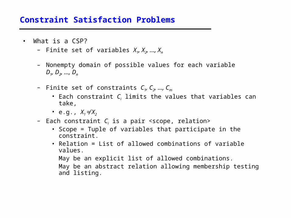
Constraint Satisfaction Problems
• What is a CSP?– Finite set of variables X1, X2, …, Xn
– Nonempty domain of possible values for each variable D1, D2, …, Dn
– Finite set of constraints C1, C2, …, Cm
• Each constraint Ci limits the values that variables can take, • e.g., X1 ≠ X2
– Each constraint Ci is a pair <scope, relation>• Scope = Tuple of variables that participate in the constraint.• Relation = List of allowed combinations of variable values.
May be an explicit list of allowed combinations.May be an abstract relation allowing membership testing and listing.

8-Queens
• Variables: Queens, one per column– Q1, Q2, …, Q8
• Domains: row placement, {1,2,…,8}
• Constraints:• Qi != Qj (j != i)• |Qi – Qj| != |i – j|
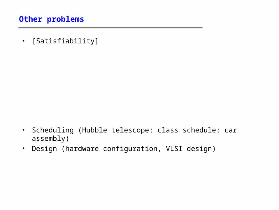
Other problems
• [Satisfiability]
• Scheduling (Hubble telescope; class schedule; car assembly)• Design (hardware configuration, VLSI design)

CSPs --- what is a solution?
• A state is an assignment of values to some or all variables.– An assignment is complete when every variable has a value. – An assignment is partial when some variables have no values.
• Consistent assignment– assignment does not violate the constraints
• A solution to a CSP is a complete and consistent assignment.
• Some CSPs require a solution that maximizes an objective function.
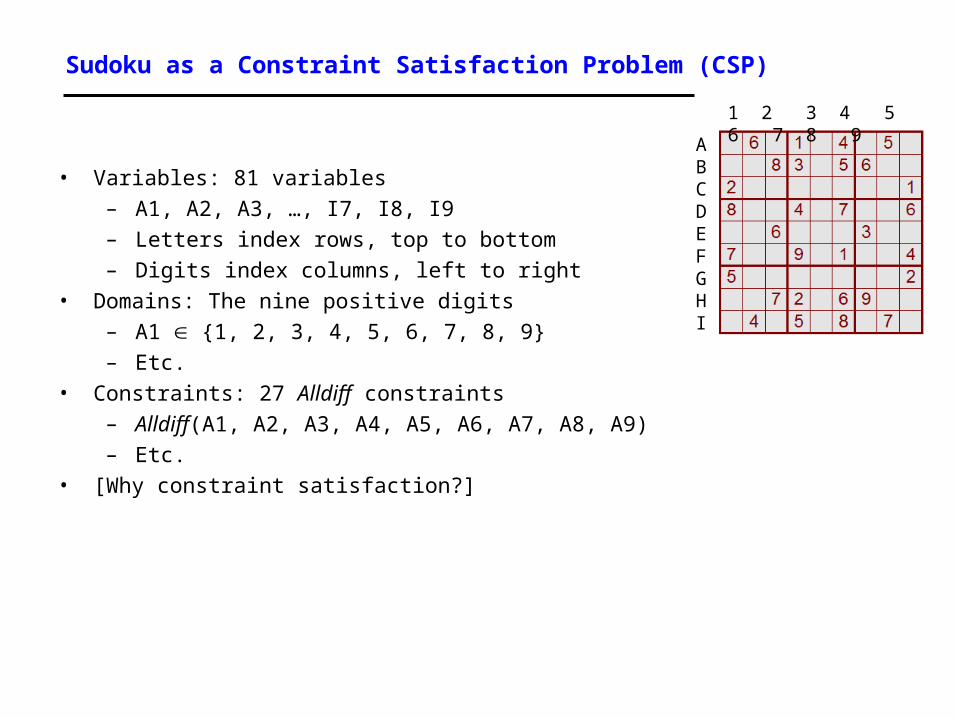
Sudoku as a Constraint Satisfaction Problem (CSP)
• Variables: 81 variables– A1, A2, A3, …, I7, I8, I9– Letters index rows, top to bottom– Digits index columns, left to right
• Domains: The nine positive digits– A1 {1, 2, 3, 4, 5, 6, 7, 8, 9}– Etc.
• Constraints: 27 Alldiff constraints– Alldiff(A1, A2, A3, A4, A5, A6, A7, A8, A9)– Etc.
• [Why constraint satisfaction?]
ABCDEFGHI
1 2 3 4 5 6 7 8 9

CSP example: map coloring
• Variables: WA, NT, Q, NSW, V, SA, T
• Domains: Di={red,green,blue}
• Constraints:adjacent regions must have different colors.• E.g. WA NT

CSP example: map coloring
• Solutions are assignments satisfying all constraints, e.g. {WA=red,NT=green,Q=red,NSW=green,V=red,SA=blue,T=green}

Constraint graphs
• Constraint graph:
• nodes are variables
• arcs are binary constraints
• Graph can be used to simplify search e.g. Tasmania is an independent subproblem

Varieties of constraints
• Unary constraints involve a single variable.– e.g. SA green
• Binary constraints involve pairs of variables.– e.g. SA WA
• Higher-order constraints involve 3 or more variables.– Professors A, B,and C cannot be on a committee together– Can always be represented by multiple binary constraints
• Preference (soft constraints) – e.g. red is better than green often can be represented by a cost for
each variable assignment – combination of optimization with CSPs

CSP Example: Cryptharithmetic puzzle

CSP Example: Cryptharithmetic puzzle

CSP as a standard search problem
• A CSP can easily be expressed as a standard search problem.
• Incremental formulation
– Initial State: the empty assignment {}
– Successor function: Assign a value to an unassigned variable provided that it does not violate a constraint
– Goal test: the current assignment is complete (by construction it is consistent)
– Path cost: constant cost for every step (not really relevant)
• Can also use complete-state formulation– Local search techniques (Chapter 4)
CSP as a standard search problem
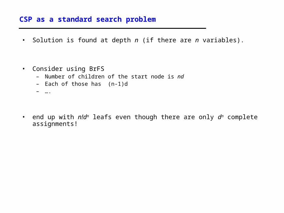
• Solution is found at depth n (if there are n variables).
• Consider using BrFS– Number of children of the start node is nd – Each of those has (n-1)d– ….
• end up with n!dn leafs even though there are only dn complete assignments!

Commutativity
• CSPs are commutative.
– The order of any given set of actions has no effect on the outcome.
– Another Example: choose colors for Australian territories one at a time
• [WA=red then NT=green] same as [NT=green then WA=red]
• All CSP search algorithms can generate successors by considering assignments for only a single variable on each level there are dn leaves
(will need to figure out later which variable to assign a value to at each node)

Backtracking search
• Depth-first searchin the context of CSP is also called “backtracking”• Chooses values for one variable at a time and backtracks when a
variable has no legal values left to assign.• Nice: we have a standard representation. No need for a domain-
specific initial state, successor function, or goal test.

Backtracking search
function BACKTRACKING-SEARCH(csp) return a solution or failurereturn BACKTRACK({} , csp)
function BACKTRACK(assignment, csp) return a solution or failureif assignment is complete then return assignmentvar SELECT-UNASSIGNED-VARIABLE(csp,assignment)for each value in ORDER-DOMAIN-VALUES(var, assignment, csp) do
if value is consistent with assignment thenadd {var=value} to assignment
inferences INFERENCE(csp,assignment)if inferences != failure
add inferences to assignment result BACTRACK(assignment, csp)
if result failure then return resultremove {var=value} and inferences from assignment (if you added it)
return failure

Improving CSP efficiency
• Previous improvements on uninformed search introduce heuristics
• For CSPS, general-purpose methods can give large gains in speed, e.g.,– Which variable should be assigned next?– In what order should its values be tried?– Can we detect inevitable failure early?

Backtracking search
SELECT-UNASSIGNED-VARIABLE• Minimum Remaining Values (MRV)
– Most constrained variable– Most likely to fail soon (so prunes pointless searches)
• If a tie (such as choosing the start state), choose the variable involved in the most constraints (degree heuristic) E.g., in the map example, SA adjacent to the most states.– Reduces branching factor, since fewer legal successors of that node

CSP example: map coloring
• Solutions are assignments satisfying all constraints, e.g. {WA=red,NT=green,Q=red,NSW=green,V=red,SA=blue,T=green}

Backtracking search
ORDER-DOMAIN-VALUES– Least Constraining Value– Rules out the fewest choices for the variables it is in constraints
with– Leave the maximum flexibility– You’ve chosen the variable, now let’s make the most of it

Minimum remaining values (MRV)
var SELECT-UNASSIGNED-VARIABLE(assignment,csp)
– Before the assignment to the rightmost state: one region has one remaining; one region has two; three regions have three. Choose the region with only one remaining
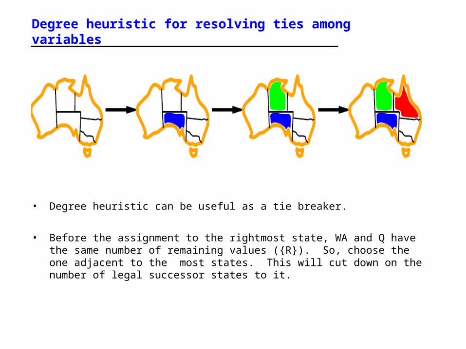
Degree heuristic for resolving ties among variables
• Degree heuristic can be useful as a tie breaker.
• Before the assignment to the rightmost state, WA and Q have the same number of remaining values ({R}). So, choose the one adjacent to the most states. This will cut down on the number of legal successor states to it.

Least constraining value for value-ordering
• Least constraining value heuristic
• Heuristic Rule: given a variable choose the least constraining value– leaves the maximum flexibility for subsequent variable assignments

Forward checking (INFERENCE)
• Can we detect inevitable failure early?– And avoid it later?
• Forward checking idea: keep track of remaining legal values for unassigned variables.
• Terminate search when any variable has no legal values.

Forward checking
• Assign {WA=red}
• Effects on other variables connected by constraints to WA– NT can no longer be red– SA can no longer be red
• Note: this example is not using MRV; if it were, we would choose NT or SA next. But, we will choose Q next. This example is from the text. It shows the example here, then talks through what would happen if we had used MRV.

Forward checking
• Assign {Q=green}
• Effects on other variables connected by constraints with WA– NT can no longer be green– NSW can no longer be green– SA can no longer be green

Forward checking
• Assign {V=blue}
• Effects on other variables connected by constraints with WA– NSW can no longer be blue– SA is empty
• Forward Checking has detected that partial assignment is inconsistent with the constraints and backtracking can occur.

Backtracking search
function BACKTRACKING-SEARCH(csp) return a solution or failurereturn BACKTRACK({} , csp)
function BACKTRACK(assignment, csp) return a solution or failureif assignment is complete then return assignmentvar SELECT-UNASSIGNED-VARIABLE(csp,assignment)for each value in ORDER-DOMAIN-VALUES(var, assignment, csp) do
if value is consistent with assignment thenadd {var=value} to assignment
inferences INFERENCE(csp,assignment)if inferences != failure
add inferences to assignment result BACTRACK(assignment, csp)
if result failure then return resultremove {var=value} and inferences from assignment (if you added it)
return failure

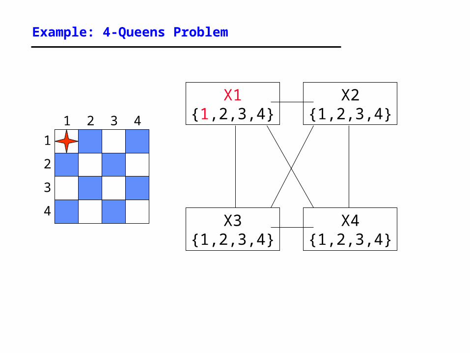
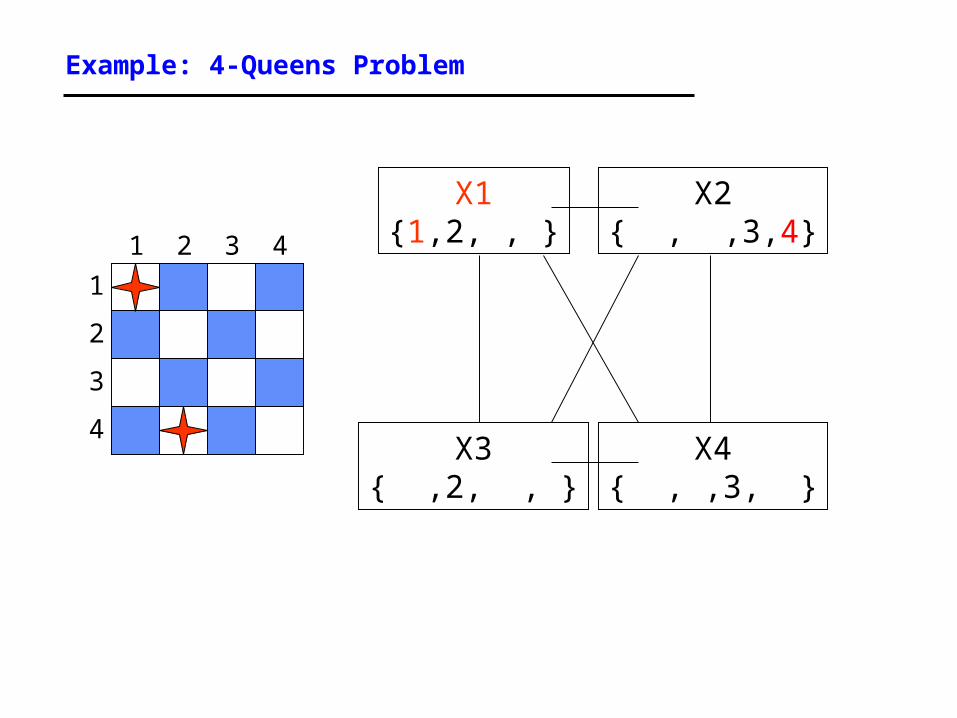
Example: 4-Queens Problem
1
3
2
4
32 41
X1{1,2,3,4}
X3{1,2,3,4}
X4{1,2,3,4}
X2{1,2,3,4}
Example: 4-Queens Problem
1
3
2
4
32 41
X1{1,2,3,4}
X3{1,2,3,4}
X4{1,2,3,4}
X2{1,2,3,4}

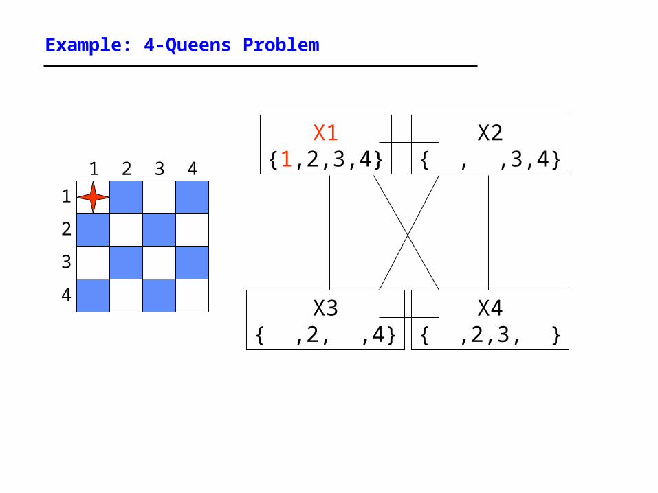
Example: 4-Queens Problem
1
3
2
4
32 41
X1{1,2,3,4}
X3{ ,2, ,4}
X4{ ,2,3, }
X2{ , ,3,4}

Example: 4-Queens Problem
1
3
2
4
32 41
X1{1, , , }
X3{ , , , }
X4{ ,2, , }
X2{ , ,3,4}
Example: 4-Queens Problem
1
3
2
4
32 41
X1{1,2,3,4}
X3{ ,2, ,4}
X4{ ,2,3, }
X2{ , ,3,4}

Example: 4-Queens Problem
1
3
2
4
32 41
X1{1,2,3,4}
X3{ ,2, , }
X4{ ,2,3, }
X2{ , ,3,4}
Example: 4-Queens Problem
1
3
2
4
32 41
X1{1,2, , }
X3{ ,2, , }
X4{ , ,3, }
X2{ , ,3,4}

Example: 4-Queens Problem
1
3
2
4
32 41
X1{1,2, , }
X3{ ,2, , }
X4{ , ,3, }
X2{ , ,3,4}

Example: 4-Queens Problem
1
3
2
4
32 41
X1{1, , , }
X3{ ,2, , }
X4{ , , , }
X2{ , , ,4}

Solving CSPs (backtrack) with combination of heuristics plus forward checking is more efficient than either approach alone
But Forward Checking does not see all inconsistencies
Consider our map coloring search, after we have assigned WA=red and Q=green

Forward checking
• WA=Red; Q=green• Forward checking gives us the third row
• At this point, we can see that this is inconsistent, since NT and SA are forced to be blue, yet they are adjacent. Forward checking doesn’t see this, and proceeds onward in the search from this state (as we saw earlier)
Constraint propagation
• Forward checking (FC) is in effect eliminating parts of the search space
• Constraint propagation goes further than FC by repeatedly enforcing constraints locally– Needs to be faster than actually searching to be effective
• Arc-consistency (AC) is a systematic procedure for constraint propagation

Arc consistency
• An Arc X Y is consistent iffor every value x of X there is some value y consistent with x
• Consider state of search after WA and Q are assigned:
SA NSW is consistent: if SA=blue NSW could be =red
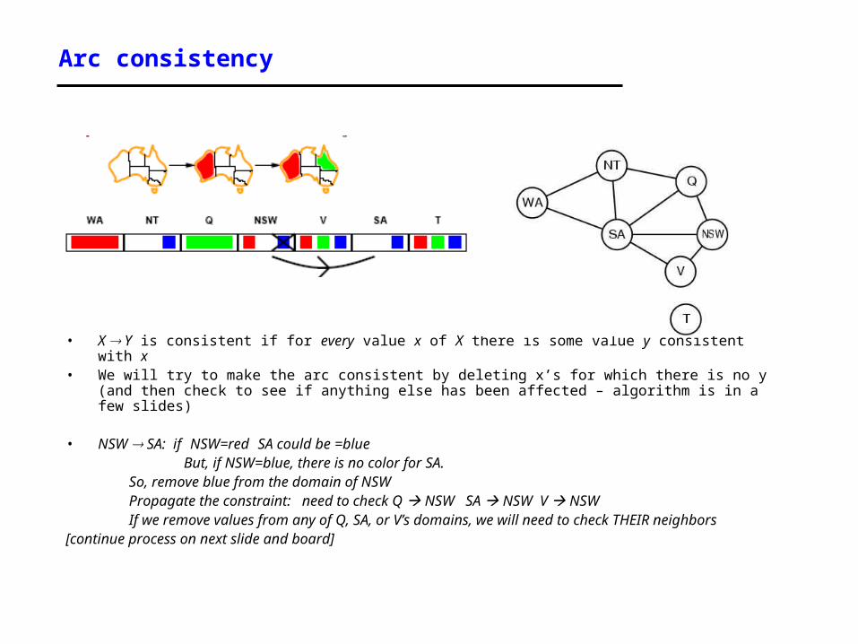
Arc consistency
• X Y is consistent if for every value x of X there is some value y consistent with x• We will try to make the arc consistent by deleting x’s for which there is no y (and then check to
see if anything else has been affected – algorithm is in a few slides)
• NSW SA: if NSW=red SA could be =blueBut, if NSW=blue, there is no color for SA.
So, remove blue from the domain of NSW Propagate the constraint: need to check Q NSW SA NSW V NSW If we remove values from any of Q, SA, or V’s domains, we will need to check THEIR
neighbors[continue process on next slide and board]
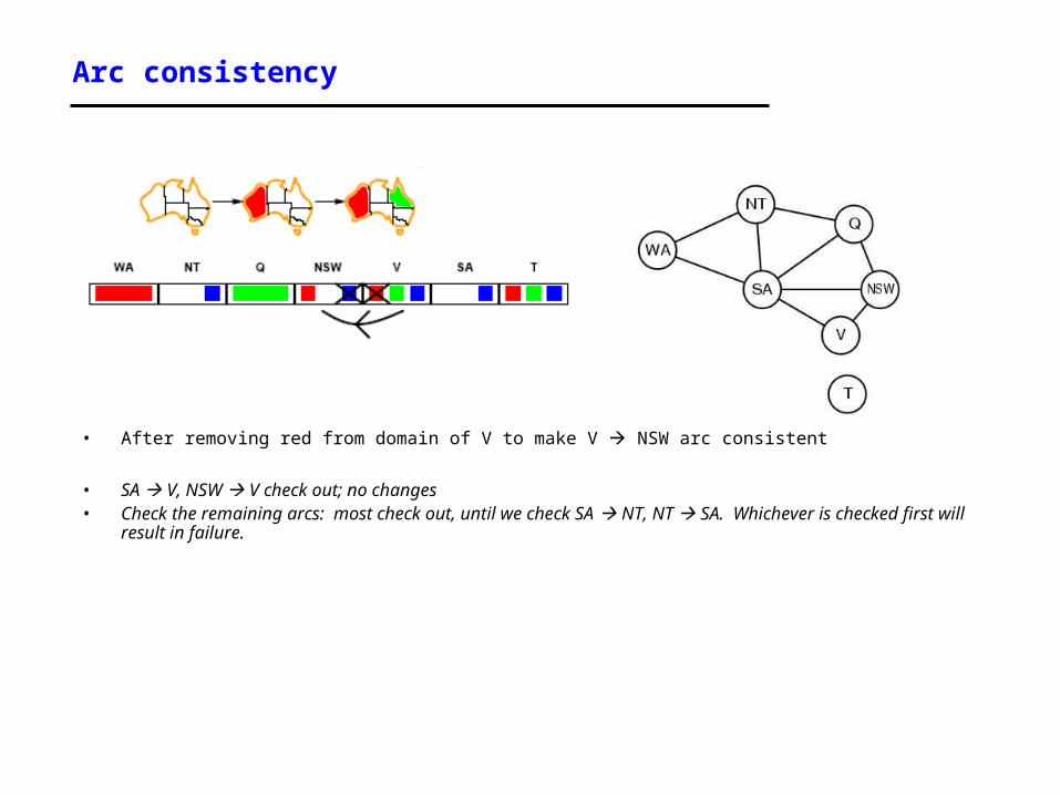
Arc consistency
• After removing red from domain of V to make V NSW arc consistent
• SA V, NSW V check out; no changes• Check the remaining arcs: most check out, until we check SA NT, NT SA. Whichever is
checked first will result in failure.
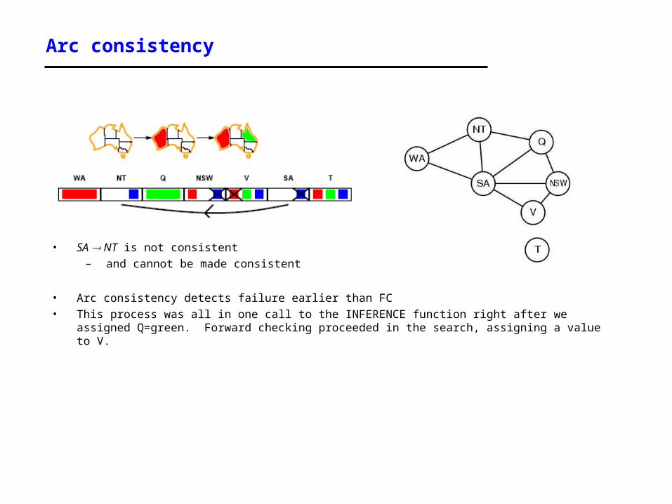
Arc consistency
• SA NT is not consistent
– and cannot be made consistent
• Arc consistency detects failure earlier than FC• This process was all in one call to the INFERENCE function right after we assigned Q=green.
Forward checking proceeded in the search, assigning a value to V.
Arc consistency checking
• AC must be run until no inconsistency remains
• Trade-off– Requires some overhead to do, but generally more effective than direct search– In effect it can eliminate large (inconsistent) parts of the state space more effectively
than search can
• Need a systematic method for arc-checking – If X loses a value, neighbors of X need to be rechecked:
i.e. incoming arcs can become inconsistent again (outgoing arcs will stay consistent).
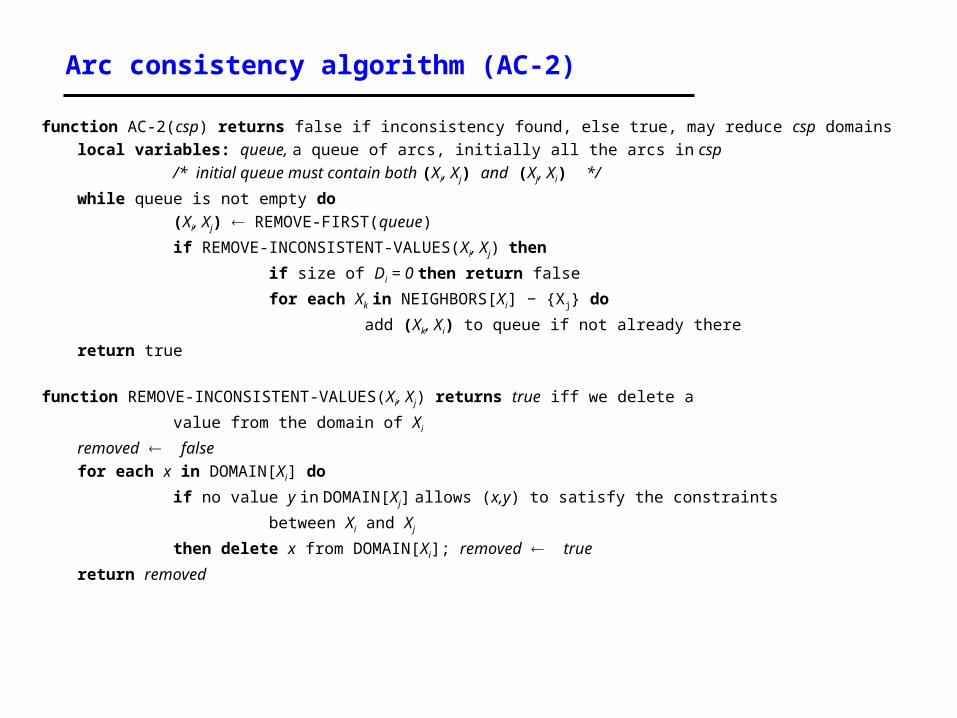
Arc consistency algorithm (AC-2)
function AC-2(csp) returns false if inconsistency found, else true, may reduce csp domainslocal variables: queue, a queue of arcs, initially all the arcs in csp
/* initial queue must contain both (Xi, Xj) and (Xj, Xi) */
while queue is not empty do(Xi, Xj) REMOVE-FIRST(queue)
if REMOVE-INCONSISTENT-VALUES(Xi, Xj) then
if size of Di = 0 then return false
for each Xk in NEIGHBORS[Xi] − {Xj} do
add (Xk, Xi) to queue if not already there
return true
function REMOVE-INCONSISTENT-VALUES(Xi, Xj) returns true iff we delete a
value from the domain of Xi
removed falsefor each x in DOMAIN[Xi] do
if no value y in DOMAIN[Xj] allows (x,y) to satisfy the constraints
between Xi and Xj
then delete x from DOMAIN[Xi]; removed true
return removed

Complexity of AC-2
• A binary CSP has at most n2 arcs
• Each arc can be inserted in the queue d times (worst case)– (X, Y): only d values of X to delete
• Consistency of an arc can be checked in O(d2) time (d values of the first * d values of the second)
• Complexity is O(n2 d3)
• Although substantially more expensive than Forward Checking, Arc Consistency is usually worthwhile.

Trade-offs
• Running stronger consistency checks…– Takes more time– But will reduce branching factor and detect more inconsistent partial assignments
– No “free lunch” • In worst case n-consistency takes exponential time
• Generally helpful to enforce 2-Consistency (Arc Consistency)
• Sometimes helpful to enforce 3-Consistency
• Higher levels may take more time to enforce than they save.
Local search for CSPs
• Use complete-state representation– Initial state = all variables assigned values– Successor states = change a value
• For CSPs– allow states with unsatisfied constraints (unlike backtracking)– operators reassign variable values– hill-climbing with n-queens is an example (we saw in earlier notes)
• Variable selection: randomly select any conflicted variable
• Value selection: min-conflicts heuristic– Select new value that results in a minimum number of conflicts with the other variables

Local search for CSP
function MIN-CONFLICTS(csp, max_steps) return solution or failureinputs: csp, a constraint satisfaction problem
max_steps, the number of steps allowed before giving up
current an initial complete assignment for cspfor i = 1 to max_steps do
if current is a solution for csp then return currentvar a randomly chosen, conflicted variable from VARIABLES[csp]value the value v for var that minimize
CONFLICTS(var,v,current,csp)set var = value in current
return failure
Min-conflicts example
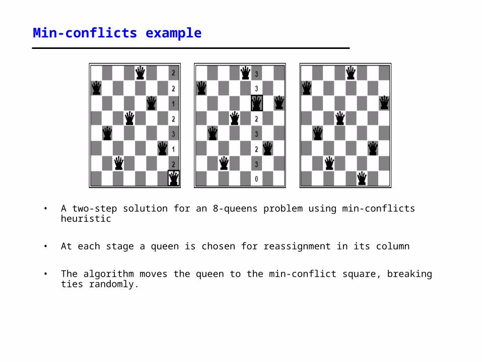
• A two-step solution for an 8-queens problem using min-conflicts heuristic
• At each stage a queen is chosen for reassignment in its column
• The algorithm moves the queen to the min-conflict square, breaking ties randomly.

Advantages of local search
• Local search can be particularly useful in an online setting– Airline schedule example
• E.g., mechanical problems require that a plane is taken out of service• Can locally search for another “close” solution in state-space• Much better (and faster) in practice than finding an entirely new schedule
• The runtime of min-conflicts is roughly independent of problem size for the 8-queens (observation in the 1990’s that gave rise to much research).
– Can solve the millions-queen problem in roughly 50 steps.– Why?
• n-queens is easy for local search because of the relatively high density of solutions in state-space

Summary
• CSPs – special kind of problem: states defined by values of a fixed set of variables,
goal test defined by constraints on variable values
• Backtracking=depth-first search with one variable assigned per level
• Heuristics– Variable ordering and value selection heuristics help significantly
• Constraint propagation does additional work to constrain values and detect inconsistencies
– Works effectively when combined with heuristics
• Iterative min-conflicts is often effective in practice.

Wrapup: You Will Be Expected to Know
• Basic definitions (section 6.1)
• Arc consistency (6.2.2); Sudoku example (6.2.6)
• Backtracking search (6.3)
• Variable and value ordering: minimum-remaining values, degree heuristic, least-constraining-value (6.3.1)
• Forward checking (6.3.2)
• Local search for CSPs: min-conflict heuristic (6.4)