Constraining Cosmology with Lyman-alpha Emitters - a Study ...
153
Constraining Cosmology with Lyman-alpha Emitters a Study Using HETDEX Parameters Ralf Koehler M¨ unchen 2009
Transcript of Constraining Cosmology with Lyman-alpha Emitters - a Study ...

Constraining Cosmology withLyman-alpha Emitters
a Study Using HETDEX Parameters
Ralf Koehler
Munchen 2009

Constraining Cosmology withLyman-alpha Emitters
a Study Using HETDEX Parameters
Ralf Koehler
Dissertation
an der Fakultat fur Physik
der Ludwig–Maximilians–Universitat
Munchen
vorgelegt von
Ralf Koehler
aus Munchen
Munchen, den 20.01.2009

Erstgutachter: Prof. Dr. Ralf Bender
Zweitgutachter: Prof. Dr. Jochen Weller
Tag der mundlichen Prufung: 23.04.2009

Contents
Zusammenfassung xiii
Abstract xiv
1 Introduction 1
1.1 Motivation . . . . . . . . . . . . . . . . . . . . . . . . . . . . . . . . . . . . 1
1.2 Power Spectrum Cosmology . . . . . . . . . . . . . . . . . . . . . . . . . . 2
1.2.1 Power Spectrum . . . . . . . . . . . . . . . . . . . . . . . . . . . . . 2
1.2.2 Geometry . . . . . . . . . . . . . . . . . . . . . . . . . . . . . . . . 3
1.2.3 Growth . . . . . . . . . . . . . . . . . . . . . . . . . . . . . . . . . 4
1.3 Lyman Alpha Emitters . . . . . . . . . . . . . . . . . . . . . . . . . . . . . 5
1.3.1 Biasing . . . . . . . . . . . . . . . . . . . . . . . . . . . . . . . . . . 5
1.3.2 Contamination . . . . . . . . . . . . . . . . . . . . . . . . . . . . . 6
1.4 Dark Energy . . . . . . . . . . . . . . . . . . . . . . . . . . . . . . . . . . . 6
1.5 HETDEX . . . . . . . . . . . . . . . . . . . . . . . . . . . . . . . . . . . . 7
1.5.1 VIRUS . . . . . . . . . . . . . . . . . . . . . . . . . . . . . . . . . . 8
1.5.2 The Survey . . . . . . . . . . . . . . . . . . . . . . . . . . . . . . . 8
1.5.3 Cosmology . . . . . . . . . . . . . . . . . . . . . . . . . . . . . . . . 9
1.5.4 VIRUS-P . . . . . . . . . . . . . . . . . . . . . . . . . . . . . . . . 10
1.6 Overview . . . . . . . . . . . . . . . . . . . . . . . . . . . . . . . . . . . . . 11
2 Probing Dark Energy with Baryonic Acoustic Oscillations 13
2.1 Introduction . . . . . . . . . . . . . . . . . . . . . . . . . . . . . . . . . . . 13
2.2 Baryonic Acoustic Oscillations (BAOs) . . . . . . . . . . . . . . . . . . . . 15
2.3 Extracting BAOs under Linear Conditions . . . . . . . . . . . . . . . . . . 19
2.4 Extracting BAOs under Quasi-Nonlinear Conditions . . . . . . . . . . . . . 23
2.5 Extracting BAOs in Redshift Space . . . . . . . . . . . . . . . . . . . . . . 30
2.6 Extracting BAOs from Biased Samples . . . . . . . . . . . . . . . . . . . . 34
2.7 Cosmological Tests with BAOs . . . . . . . . . . . . . . . . . . . . . . . . . 37
2.8 Discussion and Conclusions . . . . . . . . . . . . . . . . . . . . . . . . . . 43

vi CONTENTS
3 The Impact of Sparse Sampling on Power Spectrum Cosmology 45
3.1 Introduction . . . . . . . . . . . . . . . . . . . . . . . . . . . . . . . . . . . 45
3.2 The Simulations . . . . . . . . . . . . . . . . . . . . . . . . . . . . . . . . . 46
3.3 Selection Functions . . . . . . . . . . . . . . . . . . . . . . . . . . . . . . . 47
3.3.1 Radial Window Function . . . . . . . . . . . . . . . . . . . . . . . . 48
3.3.2 Angular Window Function . . . . . . . . . . . . . . . . . . . . . . . 49
3.3.3 Luminosity Calibration . . . . . . . . . . . . . . . . . . . . . . . . . 52
3.3.4 Cartesian Window Function . . . . . . . . . . . . . . . . . . . . . . 52
3.3.5 Samples . . . . . . . . . . . . . . . . . . . . . . . . . . . . . . . . . 54
3.4 Error Analysis . . . . . . . . . . . . . . . . . . . . . . . . . . . . . . . . . . 55
3.4.1 Systematic Errors . . . . . . . . . . . . . . . . . . . . . . . . . . . . 55
3.4.2 Statistical Errors . . . . . . . . . . . . . . . . . . . . . . . . . . . . 59
3.4.3 Correlation Matrix . . . . . . . . . . . . . . . . . . . . . . . . . . . 61
3.5 Cosmological Test . . . . . . . . . . . . . . . . . . . . . . . . . . . . . . . . 63
3.5.1 Geometric Test . . . . . . . . . . . . . . . . . . . . . . . . . . . . . 63
3.5.2 Growth Test . . . . . . . . . . . . . . . . . . . . . . . . . . . . . . . 64
3.5.3 Test Setup . . . . . . . . . . . . . . . . . . . . . . . . . . . . . . . . 65
3.5.4 Results . . . . . . . . . . . . . . . . . . . . . . . . . . . . . . . . . . 66
3.6 Conclusions . . . . . . . . . . . . . . . . . . . . . . . . . . . . . . . . . . . 70
4 Estimating galaxy bias in pencil-beam surveys with low point densities 73
4.1 Introduction . . . . . . . . . . . . . . . . . . . . . . . . . . . . . . . . . . . 73
4.2 Survey Layouts . . . . . . . . . . . . . . . . . . . . . . . . . . . . . . . . . 74
4.3 Estimators . . . . . . . . . . . . . . . . . . . . . . . . . . . . . . . . . . . . 76
4.3.1 Power Spectrum . . . . . . . . . . . . . . . . . . . . . . . . . . . . . 76
4.3.2 Correlation Function . . . . . . . . . . . . . . . . . . . . . . . . . . 77
4.4 Analytical Error Analysis of 3D Power Spectra . . . . . . . . . . . . . . . . 77
4.5 Low Point Density Performance . . . . . . . . . . . . . . . . . . . . . . . . 79
4.6 Realistic Data . . . . . . . . . . . . . . . . . . . . . . . . . . . . . . . . . . 80
4.6.1 The VIRUS-P survey . . . . . . . . . . . . . . . . . . . . . . . . . . 82
4.6.2 The Simulation . . . . . . . . . . . . . . . . . . . . . . . . . . . . . 82
4.6.3 Shapes . . . . . . . . . . . . . . . . . . . . . . . . . . . . . . . . . . 83
4.6.4 Errors . . . . . . . . . . . . . . . . . . . . . . . . . . . . . . . . . . 88
4.6.5 Window Function . . . . . . . . . . . . . . . . . . . . . . . . . . . . 92
4.6.6 Correlation Matrix . . . . . . . . . . . . . . . . . . . . . . . . . . . 94
4.7 Bias Determination . . . . . . . . . . . . . . . . . . . . . . . . . . . . . . . 97
4.7.1 χ2-Test . . . . . . . . . . . . . . . . . . . . . . . . . . . . . . . . . . 98
4.7.2 Results . . . . . . . . . . . . . . . . . . . . . . . . . . . . . . . . . . 98
4.8 Conclusions . . . . . . . . . . . . . . . . . . . . . . . . . . . . . . . . . . . 100

CONTENTS vii
5 The CURE Pipeline 1035.1 Introduction . . . . . . . . . . . . . . . . . . . . . . . . . . . . . . . . . . . 1035.2 Generic Reduction . . . . . . . . . . . . . . . . . . . . . . . . . . . . . . . 1045.3 Modelling Fibers . . . . . . . . . . . . . . . . . . . . . . . . . . . . . . . . 104
5.3.1 Modelling Fiber Positions . . . . . . . . . . . . . . . . . . . . . . . 1045.3.2 Modelling Fiber Profiles . . . . . . . . . . . . . . . . . . . . . . . . 1075.3.3 Models and Reality . . . . . . . . . . . . . . . . . . . . . . . . . . . 108
5.4 Subtracting Sky . . . . . . . . . . . . . . . . . . . . . . . . . . . . . . . . . 1105.5 Detecting Emission Lines . . . . . . . . . . . . . . . . . . . . . . . . . . . . 1155.6 Testing the Pipeline . . . . . . . . . . . . . . . . . . . . . . . . . . . . . . . 1165.7 Conclusions . . . . . . . . . . . . . . . . . . . . . . . . . . . . . . . . . . . 118
6 Conclusions and Outlook 1216.1 Conclusions . . . . . . . . . . . . . . . . . . . . . . . . . . . . . . . . . . . 1216.2 Outlook . . . . . . . . . . . . . . . . . . . . . . . . . . . . . . . . . . . . . 123
Acknowledgments 134

viii CONTENTS

List of Figures
1.1 Hobby Eberly Telescope . . . . . . . . . . . . . . . . . . . . . . . . . . . . 81.2 VIRUS IFU Layout . . . . . . . . . . . . . . . . . . . . . . . . . . . . . . . 91.3 HETDEX Survey Layout . . . . . . . . . . . . . . . . . . . . . . . . . . . . 101.4 HETDEX H accuracy . . . . . . . . . . . . . . . . . . . . . . . . . . . . . . 111.5 The VIRUS Prototype . . . . . . . . . . . . . . . . . . . . . . . . . . . . . 12
2.1 Transfer function . . . . . . . . . . . . . . . . . . . . . . . . . . . . . . . . 182.2 Template corrections . . . . . . . . . . . . . . . . . . . . . . . . . . . . . . 222.3 Matter power spectra and transfer functions . . . . . . . . . . . . . . . . . 242.4 Wiggles in real space . . . . . . . . . . . . . . . . . . . . . . . . . . . . . . 272.5 Extraction of different primordial power spectra . . . . . . . . . . . . . . . 282.6 Extraction from analytical function . . . . . . . . . . . . . . . . . . . . . . 292.7 Oscillations at low redshift . . . . . . . . . . . . . . . . . . . . . . . . . . . 302.8 Redshift space effects . . . . . . . . . . . . . . . . . . . . . . . . . . . . . . 312.9 Wiggles in redshift space . . . . . . . . . . . . . . . . . . . . . . . . . . . . 322.10 Wiggles in redshift space . . . . . . . . . . . . . . . . . . . . . . . . . . . . 332.11 Biased wiggles . . . . . . . . . . . . . . . . . . . . . . . . . . . . . . . . . . 352.12 Biased wiggles . . . . . . . . . . . . . . . . . . . . . . . . . . . . . . . . . . 362.13 w0 scaling . . . . . . . . . . . . . . . . . . . . . . . . . . . . . . . . . . . . 382.14 Scaled transfer functions . . . . . . . . . . . . . . . . . . . . . . . . . . . . 392.15 Combined wiggles . . . . . . . . . . . . . . . . . . . . . . . . . . . . . . . . 412.16 Cosmological test results . . . . . . . . . . . . . . . . . . . . . . . . . . . . 42
3.1 Mean power spectrum of 400 cubes . . . . . . . . . . . . . . . . . . . . . . 483.2 Radial selection function . . . . . . . . . . . . . . . . . . . . . . . . . . . . 493.3 Angular selection function . . . . . . . . . . . . . . . . . . . . . . . . . . . 503.4 Angular window function . . . . . . . . . . . . . . . . . . . . . . . . . . . . 513.5 Breaking of distant observer relation . . . . . . . . . . . . . . . . . . . . . 533.6 2D Log window function . . . . . . . . . . . . . . . . . . . . . . . . . . . . 543.7 Power spectral ratios . . . . . . . . . . . . . . . . . . . . . . . . . . . . . . 563.8 Convoluted power spectra . . . . . . . . . . . . . . . . . . . . . . . . . . . 583.9 Zero-point correction . . . . . . . . . . . . . . . . . . . . . . . . . . . . . . 593.10 Relative Errors . . . . . . . . . . . . . . . . . . . . . . . . . . . . . . . . . 60

x LIST OF FIGURES
3.11 Correlation Matrices . . . . . . . . . . . . . . . . . . . . . . . . . . . . . . 623.12 χ2 results of undistorted sample . . . . . . . . . . . . . . . . . . . . . . . . 673.13 χ2 test results comparing distorting effects . . . . . . . . . . . . . . . . . . 683.14 χ2 test results comparing errors and correlations . . . . . . . . . . . . . . . 693.15 Artificial systematic errors . . . . . . . . . . . . . . . . . . . . . . . . . . . 703.16 χ2 test with systematic errors . . . . . . . . . . . . . . . . . . . . . . . . . 71
4.1 Mean power spectra of samples with variing point densities . . . . . . . . . 814.2 Mean correlation functions of samples with variing point densities . . . . . 814.3 Radial VIRUS-P selection function . . . . . . . . . . . . . . . . . . . . . . 824.4 Mean power spectra of samples with variing angular diameter using a cube 854.5 Mean power spectra of samples with variing angular diameter using a cuboid 854.6 Mean correlation functions of samples with variing angular diameter . . . . 864.7 Mean power spectra of samples with variing point densities using cubes . . 864.8 Mean power spectra of samples with variing point densities using cuboids . 874.9 Mean correlation functions of samples with variing point densities . . . . . 874.10 Power spectral errors of samples with variing angular diameter using cubes 884.11 Power spectral errors of samples with variing angular diameter using cuboids 894.12 Correlation function errors of samples with variing angular diameter . . . . 904.13 Power spectral errors compared with theoretical rpedictions . . . . . . . . 914.14 Window functions of samples with varring angular diameter in the FFT cube 934.15 Window functions of samples with varring angular diameter in the FFT cuboid 934.16 Autocorrelation functions of samples with variing angular diameter . . . . 944.17 Correlation matrices . . . . . . . . . . . . . . . . . . . . . . . . . . . . . . 954.18 Zoomed in correlation matrices . . . . . . . . . . . . . . . . . . . . . . . . 964.19 χ2 results . . . . . . . . . . . . . . . . . . . . . . . . . . . . . . . . . . . . 99
5.1 Flow diagram . . . . . . . . . . . . . . . . . . . . . . . . . . . . . . . . . . 1055.2 Masterarc fits file . . . . . . . . . . . . . . . . . . . . . . . . . . . . . . . . 1065.3 Mastertrace fits file . . . . . . . . . . . . . . . . . . . . . . . . . . . . . . . 1075.4 Fiber profiles . . . . . . . . . . . . . . . . . . . . . . . . . . . . . . . . . . 1095.5 Breathing of distortion pattern . . . . . . . . . . . . . . . . . . . . . . . . 1105.6 CURE sky re-construction . . . . . . . . . . . . . . . . . . . . . . . . . . . 1115.7 Sky versus no-sky data . . . . . . . . . . . . . . . . . . . . . . . . . . . . . 1125.8 Statistics of empty resolution elements . . . . . . . . . . . . . . . . . . . . 1145.9 PSF standard deviations . . . . . . . . . . . . . . . . . . . . . . . . . . . . 1165.10 Detected Lyman-alpha emitters . . . . . . . . . . . . . . . . . . . . . . . . 1175.11 CURE detection efficiency . . . . . . . . . . . . . . . . . . . . . . . . . . . 1185.12 CURE detection accuracy . . . . . . . . . . . . . . . . . . . . . . . . . . . 119

List of Tables
2.1 Power spectrum cubes . . . . . . . . . . . . . . . . . . . . . . . . . . . . . 25
3.1 Pinocchio Parameters . . . . . . . . . . . . . . . . . . . . . . . . . . . . . . 473.2 CAMB Parameters . . . . . . . . . . . . . . . . . . . . . . . . . . . . . . . 65
4.1 Properties of low density samples . . . . . . . . . . . . . . . . . . . . . . . 804.2 Cosmological Parameters of the Hubble Volume Simulation . . . . . . . . . 834.3 Properties of the geometry and density test samples . . . . . . . . . . . . . 834.4 Accuracies of amplitude estimates . . . . . . . . . . . . . . . . . . . . . . . 100

xii LIST OF TABLES

Zusammenfassung
Diese Dissertation befasst sich mit den technischen Aspekten der Messung und Auswer-tung von Leistungspektren von weit entfernten Galaxien um mit deren Hilfe kosmologischeParameter einzugrenzen.
Wir untersuchen die Methode der Extraktion von baryonischen Akkustischen Oszilla-tionen (BAOs) aus dem Leistungsspektrum von Lyman-alpha emittierenden Galaxien aufseine Stabilitat und Anfalligkeit fur Fehler. Dazu schlagen wir ein parametrisches Verfahrenvor um BAOs ohne Wissen um den genauen Inhalt des Universums zu extrahieren. Wirbenutzen die Hubble Volume Simulationen um zu zeigen, dass auf diese Weise extrahierteBAOs auch trotz vorhandener Rotverschiebungseffekte, nicht linearem Wachstum und ohneKenntnis des Bias einen zuverlassigen Datensatz darstellen. Wir zeigen, dass die Oszilla-tionslange der BAOs verwendet werden kann um in einem geometrischen Test robusteResultate uber verschiedene kosmologische Modelle zu erhalten. Wir untersuchen denEinfluss von grobmaschigen Abtastmethoden auf die Fahigkeit die Amplitude und Formdes Leistungsspektrums innerhalb der Parameter des HETDEX Versuchs zu extrahieren.Dazu simulieren 400 Kuben mit einer Seitenlange von 500h−1Mpc und zeigen, dass selbsteine extrem inhomogene Fensterfunktion und der Einfluss von Kalibirierungsfehlern, denInformationsgehalt des Datensatzes nur wenig veranden. Obwohl das Leistungsspektrumdurch beide Effekte schwer verzerrt wird, kann das wahre Leistungsspektrum daraus ex-trahiert werden. Korrelationen die durch die Fensterfunktion und Kallibrierungsfehlereingefuhrt werden verringern die Fhigkeit des resultierenden Leistungsspektrums kosmol-ogische Parameter einzugrenzen nur wenig. Der Unterschied zwischen den Uberdichtender Galaxienverteilung und der zu Grunde liegenden Dichteverteilung der dunklen Ma-terie, das so genannte Biasing, ist fr die Vorhersage von kosmologischen Tests mit Hilfedes Leistungsspektrum extrem wichtig. Wir untersuchen die beste Methode um den Bi-asing Faktor aus Beobachtungsdaten mit extrem langlicher Geometrie und sehr geringerPunktdichte, wie er von VIRUS-P bereit gestellt werden wird, zu extrahieren. Wir zeigen,wie das Biasing mit Hilfe von Fast Fourier Transformationen mit quaderformigen Dimen-sionen zuverlassig geschatzt werden kann, die mit den Korrelationsfunktionen desselbenDatensatzes auch gut ubereinstimmen. Zuletzt beschreiben wir die Algorithmen und dieGenauigkeit des Reduktionsprogrammes CURE, welches in der Lage ist Daten, wie sievom im HETDEX Experiment genutzten VIRUS Spektrographen bereitgestellt werden, inEchtzeit und vollstandig automatisch zu reduzieren.

xiv Abstract

Abstract
The equation of state of dark energy is currently one of the most discussed topics in as-trophysics with a large number of ongoing or planned surveys. This thesis focuses on thetechnical aspects of measuring and recovering the power spectra of distant galaxies to con-strain cosmological parameters.
We investigate the robustness of the extraction of Baryonic Acoustic Oscillations (BAOs)from the power spectrum of Lyman-alpha emitters at high redshifts. We propose a para-metric method to recover the BAOs without any specific knowledge about the actualcomposition of the universe. We use the Hubble Volume simulation to show that BAOsextracted in this way represent a robust data set, even in the presence of redshift-spaceeffects, non-linear growth and without any knowledge of biasing. We show that BAOs areable to robustly constrain cosmological models using the BAO scale as a standard ruler fora geometric test. We explore the impact of proposed sparse sampling techniques on theability to recover the amplitude and shape of the power spectrum using the parametersof the HETDEX survey. We simulate 400 with a length of 500h−1Mpc to show that thehighly inhomogeneous window function and zero-point effects do not decrease the infor-mation content of the observed data set by a large factor. Although the power spectrum isheavily distorted by both effects, the true power spectrum can be recovered. Correlationsintroduced by the window function and zero-point errors are slightly decreasing the abilityof the resulting power spectrum to constrain cosmological paremeters. The difference inoverdensities between galaxies and the underlying dark matter field, the so-called biasing,is crucial in predicting accuracy of a cosmological test using galaxies as tracer particles forthe underlying power spectrum. We investigate the best method to extract a bias estimateout of pencil-beam like surveys like the VIRUS-P survey currently under way. VIRUS-Pwill deliver a very low density data set with a highly elongated geometry. We show that thebiasing can be estimated robustly using Fast Fourier Transforms with non-equal dimensionsthat are in good agreement with results obtained facilitating the correlation function. Wefinally describe the algorithms and accuracy of the CURE pipeline that is able to reducethe data provided by the VIRUS spectrograph used in HETDEX automatically and almostin real time.

xvi Abstract

Chapter 1
Introduction
1.1 Motivation
In the last ten years, cosmology has arrived in what a lot of scientists call “precisioncosmology”. The times when only orders of magnitude results could be given are over. Atleast since the COBE (COsmic Microwave Background Explorer) mission, we are able tomeasure cosmological parameters on the percent and sometimes sub-percent niveau.
Another exciting part of the universe was discovered only recently. Also about ten yearsago Riess et al. (1998); Perlmutter et al. (1998) discovered, using light curves of supernovaeas standard candles, the accelerated expansion of the universe. We have come a long waysince that, and various models that explain the accelerated expansion have been proposed.Some invoke the infamous cosmological constant, others claim that gravity itself is notEinsteinian at large scales, some argue that the Einsteinian description is enough and themeasured expansion is only an illusion created by local inhomogeneities. But by far themost popular explanation is dark energy (see Sect. 1.4).
Whatever the explanation is, it will have a strong impact on the future evolution atthe universe. Using the dark energy description, about 75% of the energy content in theuniverse are comprised of dark energy (see Komatsu et al., 2008). In this scenario, theuniverse is no longer dominated by matter (be it dark or baryonic), but by something elsewhich we do not understand yet.
White (2007) argues, that it is not the task of astronomers to do the particle physicistsand theorists job and put a large amount of resources into experiments to measure thenature of dark energy. Other organizations, like the Dark Energy Task Force (see Albrechtet al., 2006), show that there is indeed strong interest in the astronomers community todo exactly that.
Whatever the personal opinion is, the topic of the accelerated expansion of the universeis at least controversial, and interesting. Cosmology and the evolution and fate of theuniverse have always been one of the most interesting scientific topics that are able to gaina wide audience even outside the community astronomers and even physicits. The workdone in this thesis tries to be just another small brick in the theoretical and experimental

2 1. Introduction
framework that will, hopefully, one day explain the nature of the cosmic expansion andgrowth history, which is, maybe, some kind of dark energy.
1.2 Power Spectrum Cosmology
Since the 1980s (see e.g. Frenk et al., 1983; Bardeen et al., 1987; Bond & Efstathiou,1987) power spectra have been extensively used and refined to discriminate between var-ious cosmological parameters. The approach is quite simple: The structure we observein the universe today, was only able to form, because small initial quantum-fluctuations(Bardeen et al., 1983). These fluctuations were blown up by inflation (see Guth, 1981)to cosmological scales, and are the perturbations in the otherwise very homogeneous uni-verse, that allowed galaxies and clusters of galaxies to form. These overdensities can bedescribed statistically using a power spectrum. We know the shape of the power spectrumof the Cosmic Microwave Background (CMB) and the initial matter density distributiondepending on various cosmological parameters (see Eisenstein & Hu, 1998), like the totalmatter content, Ωm, the dark energy content, ΩΛ, or the curvature of the universe, ΩK.Both spectra can be calculated using simple plasma physics (see Sect. 2.2).
However, the shape and amplitude can be distorted. This is caused either by the space-time geometry, through which we observe the power spectrum, or by to structure growth,which, upon other effects, enhances the amplitude of the power spectrum. Both effectscan be calculated to a degree which enables us to derive cosmological parameters to goodaccuracy by comparing the observed power spectra with theoretical predictions. The mostprominent experiments today is the Wilkinson Microwave Anisotropy Probe (WMAP),that has brought us the most accurate estimates of cosmological parameters available (seeKomatsu et al., 2008).
Much of the work in this thesis will revolve around power spectra in various coordinatesystems. It is thus useful to give a short summary of the mathematical calculation andmain attributes of power spectra.
1.2.1 Power Spectrum
Throughout this work we use a Fourier transformation convention such that the inversetransformation in real space r of a quantity in k space becomes:
δ(~r) =1
(2π)3
∫d3k δ(~k) e−i
~k·~r . (1.1)
When talking about power spectra, this work will always refer to the power spectra ofoverdensities (in the case of the Cosmic Microwave Background temperature fluctuations),δ(~r). They are readily calculated from the mean local density, ρ(~r):
δ(~r) =ρ(~r) − ρ
ρ. (1.2)

1.2 Power Spectrum Cosmology 3
The mean local density is dependent on redshift, distance to the observer and otherparameters, which are in turn dependent on the position ~r. The correlation function ξ(r)describes the correlation of the density field with itself (autocorrelation) at a given distancer:
ξ(r) = 〈δ(~r′ + ~r) δ(~r′)〉 . (1.3)
The power spectrum, P (k), is now the Fourier transform of the spatial two pointcorrelation function ξ(r), and vice versa,
P (k) =∫d3r ξ(~r) ei
~k·~r . (1.4)
With the definition of the Dirac delta distribution,
δD(~k) =1
(2π)3
∫d3r e±i
~k·~r , (1.5)
and the Fourier transformed overdensities,
δ(~k) =∫d3r δ(~r) ei
~k·~r . (1.6)
the relation between the power spectrum and the fluctuation can be expressed explicitly:
〈δ(~k) δ∗(~k′)〉 = (2π)3 P (k) δD(~k − ~k′) . (1.7)
Note that an asterisk denotes the complex conjugate. The power spectrum dependingon ~k is a direct measure of the power carried per fluctuation mode ~k.
1.2.2 Geometry
A geometrical test involves the transformation of a specific scale length, in this case thescales provided by the theoretically predicted power spectrum, depending on space-timegeometry. A power spectrum survey measures angular positions, φ, on the sky, and red-shifts, which are transformed into the co-moving coordinates, x, using a certain referencecosmology. The co-moving coordinates are used to calculate a test power spectrum, whichcan then compared to a theoretically predicted power spectrum that acts as a standardruler. The transformations for angular, x‖, and line of sight, x⊥, coordinates
x‖ =∫ z2
z1
c
H(z)dz , (1.8)
x⊥ = φ∫ z2
0
c
H(z)dz , (1.9)
depends mostly on the Hubble constant, H(z). In a flat universe, the evolution of theconstant can be expressed like:

4 1. Introduction
H(z) = H0
√Ωm (1 + z)3 + ΩΛ e
3∫ z0d ln(1+z′) [1+w(z′)] , (1.10)
with c being the speed of light and the Hubble constant today H0 ≈ 72 km
sMpc. The
measured transformed distances can than be compared to the predictions. However, it isoften easier to calculate the power spectrum only once and use a “stretching factor”, sbetween two different cosmologies to stretch it. Because we have two angular dimensionsand one line of sight dimension, the stretch factor can be calculated from the ratio of scalelengths between a reference cosmology, x and a test cosmology, x, like:
s (ΩΛ,Ωm, w) =1
3
x‖x‖
+2
3
x⊥x⊥
. (1.11)
The one dimensionally average power spectrum scales with this stretching factor asfollows,
P (k, s) = s−3 P (k s) . (1.12)
The biggest impact, the boost or reduction of amplitude is explained by the volumeindependence of the power spectrum. If the same power is detected in a larger volume, theamplitude of the power spectrum goes down and vice versa.
1.2.3 Growth
Growth measures the speed of structure growth (or growth suppression when looking back-ward in time) due to gravitational forces. On first order dark energy is delaying structuregrowth, as it leads to an acceleration of the expansion of the universe. This results instructures being formed at a later time compared to a universe without dark energy.
Linear growth can be calculated by solving the growth equation:
∂2δ
∂t2+ 2
a
a
∂δ
∂t= 4π Gρ δ , (1.13)
with G being the the gravitational constant, a the expansion factor of the universe andthe time t.
Assuming a flat universe the growth function of the growing mode can be approximated(see Peebles, 1993):
δ(t) ∼ a
a
∫ t
0
da
a3= H(z)
5 Ωm
2
∫ ∞z
1 + z′
H3(z′)dz′ = D(z) , (1.14)
with ˙ = d/dt, and the scale factor a ∝ (1 + z)−1. The power spectrum itself scaleswith the growth ratio D only in amplitude
P (~k,D) = D2(z)P (~k) . (1.15)

1.3 Lyman Alpha Emitters 5
By measuring the amplitude of the power spectrum at different times, for example atthe epoch of recombination and at a redshift of z = 1, we can pinpoint a reference cosmol-ogy, that can be compared to measurements at other redshifts to constrain cosmologicalparameters.
1.3 Lyman Alpha Emitters
Lyman-alpha emitters (LAEs) (see Charlot & Fall, 1993) are young star-forming galaxies.The mostly ultraviolet emission of young and hot stars is absorbed by neutral hydrogenand re-emitted as Lyman-alpha emission at a wavelength of 121.6nm. This absorptionand re-emission process can occur a number of times, till the radiation finally escapes thegalaxy.
The main advantage of LAEs in surveys is the ability to detect the Lyman-alpha emis-sion line of high-redshift galaxies in the visible spectrum. The emission line is much easierto detect than the galaxies of continuum emission and thus enables us to observe galaxieswhich are not accessible by any other means. After a long period of unsuccessful searchesfor LAEs, the first emitters were found in the mid 1990 (see e.g. Steidel et al., 1996; Huet al., 1998) and have led to a run for finding the most distant emitters today (see e.g.Taniguchi et al., 2005; Ota et al., 2008).
Because of their properties, LAEs are ideal tracers for the dark matter distribution athigh redshifts. However, some problems have to be solved to facilitate their full potential.
1.3.1 Biasing
The properties of Lyman-alpha emitters are still not very well understood. Although therehave been efforts to model the population and evolution of LAEs (see Delliou et al., 2006;Orsi et al., 2008), statistical properties are still not well known. Their mostly irregularshape, the fact they are young and maybe still in formation further complicates the processof understanding LAEs.
Especially important for power spectrum cosmology is the so-called biasing. It describesthe fact that galaxies tend to form only in the highest overdensities of the underlyingdark matter distribution. The amplitude of the observed power spectrum, Pobs(k) is thusboosted by the scale dependent biasing b(k), compared to the dark matter power spectrum,PDM(k):
Pobs(k) = b2(k)PDM(k) . (1.16)
Although biasing does not affect cosmological tests looking only at the scale lengths ofthe power spectrum, it seriously affects growth tests. The best biasing estimates for LAEsat the moment are summarized by Orsi et al. (2008). The error of these measurements isstill in the range of 80-100%. Knowing the biasing of the observed galaxy population is alsoimportant for the prediction of the expected observation accuracies. Some statistical errorsare not dependent on the amplitude of the power spectrum. If the amplitude of the power

6 1. Introduction
spectrum increases and these errors stay constant, the overall accuracy of the measurementincreases. As biasing enters the power spectrum as its square, a small difference in basingcan change the result by a large amount.
1.3.2 Contamination
Another problem in using the population of Lyman-alpha emitters as tracers for the under-lying dark matter density field is the possibility of contamination. LAEs are not the onlyline-emission galaxies in the targeted spectral range. OII emission lines (372.7nm) origi-nating from much closer galaxies (at lower redshift) can be mistaken for highly redshiftedLyman-alpha emission, if the spectral range is not brad enough to find the related OIIIline. Or an OIII line emission (496.1/500.7nm) could be mistaken for even higher redshiftLAEs, if the spectral resolution is not good enough to resolve the OII lines. The observedpower spectrum, Pobs(~k), is then a sum of the true LAE power spectrum, PLAE(~k) and
the OII power spectrum, POII(~ks):
Pobs(~k) = PLAE(~k) + f 2 POII(~ks). (1.17)
The OII power spectrum is stretched by a cosmology dependent stretching factor s, asthe redshift information is mistaken for LAE redshifts at the given wavelength. The sumis weighted by the fraction of contaminating OIIs, f , from the whole sample.
1.4 Dark Energy
Observations show that the acceleration of the universe seems not to decrease, like onewould expect from a matter dominated universe, but to increase. These observations aremade using and combining various techniques, like the measurement of the angular powerspectrum of the cosmic microwave background (see Komatsu et al., 2008), the observationof light curves of supernovae (see e.g. Riess et al., 2007), the distribution of galaxies onthe sky (see e.g. Cole et al., 2005; Percival et al., 2001b) or weak lensing signals of thedark matter distribution (see e.g. Hoekstra et al., 2006). The expansion of the universe isexpressed by Einsteins field equation:
a
a= −4
3πG (ρ + 3p) , (1.18)
w =p
ρ, (1.19)
with the density, ρ, and pressure, p, of the dominant constituent of the universe. Theparameter w is the equation-of-state parameter (see Turner & White, 1997). One caneasily see, that a w value, smaller than -1/3 leads to a positive acceleration a
a.
Various forms of solutions have been proposed for the problem that known today as“dark energy” (see e.g. Peebles & Ratra, 2003).

1.5 HETDEX 7
The first solution proposed was the Cosmological Constant (see e.g. Copeland et al.,2006), introduced and later dismissed by Einstein himself. A Cosmological Constant has aw-value of exactly -1. The biggest problem of a cosmological Constant is that it can not beexplained by any means in the modern theoretical framework (see Weinberg, 1989). Thebest explanation, the zero-point energy of vacuum , is off by 120 order of magnitude.
Another explanation are various forms of scalar or vector fields, called dark energy,quintessence, k-essence, or phantom energy (see e.g. Copeland et al., 2006). They vary,upon other things, in their w-value both in absolute value and in time. Depending on themodel, they solve issues like the question why the dark energy density is comparable to thedark matter density today, which means that it has to be extremely fine tuned at earliertimes in the universe. All scalar field solutions are similar to the scalar fields responsiblefor the primordial inflation of the universe.
A further theory claims that Einsteinian gravity itself does not hold at the very largescales of the universe. It is called Modified Gravity (see e.g. Nojiri & Odintsov, 2006)and expands Einsteinian gravity at large scales, while maintaining the limits we get fromconstraints in the solar system at small scales.
More exotic solutions can be found using string theory. The braneworld model (see e.g.Shani & Shtanov, 2003) describes our universe as a 3-dimensional brane that is embeddedin a 4 or more dimensional bulk. All forces except gravity stay on our brane, while gravity isleaking into the bulk and can thus generate phenomena like the ones observed and termed“dark energy”.
Finally, some models claim that one does not need any new scalar fields, dimensions ormodified gravity it all. The so called backreaction models (see e.g. Kolb et al., 2006) claim,thatlarge scale inhomogeneities make is believe that the close universe (both in space andtime) is expanding faster than the more distant (both in scape and time) universe.
At the moment only astronomical observations probing the geometry and growth rateof the structure of the universe seem to have the power to discriminate between the variousproposed models.
1.5 HETDEX
The Hobby-Eberly-Telescope (see Fig. 1.1), located in West Texas, has one of the largestconstructed mirrors with a dimension of 11.1 times 9.8 meters. However, only about 9.2meffective aperture is used at any given moment, as the telescope tracks elevation by movingthe tracker instead of the mirror. It is thus ideally suited to do surveys of certain fractionsof the sky.
HETDEX, the Hobby-Eberly-Telescope Dark Energy eXperiment, is designed to survey0.8 million Lyman-alpaha emitters at a redshift range of 1.9 < z 3.5 to measure their powerspectrum and constrain the expansion and growth history of the universe. It was originallydesigned to measure the constant and time dependent term of w, but has just started tolook at other ways to constrain cosmological parameters using the expected data set.

8 1. Introduction
Figure 1.1: The Hobby Eberly Telescope
1.5.1 VIRUS
To achieve this, HETDEX will build and facilitate the Visible Integral-Field ReplicableUnit Spectrograph (VIRUS).
The VIRUS consists of about 92 wide-field integral-field units (IFUs) consisting ofabout 500 fibers each. The fibers are fed to 184 spectrographs with a resolution of R ≈800 and a spectral range of 350 to 550 nm. Each fiber will have a diameter of ∼ 1.5arsecs with a somewhat larger separation between each fiber, leading to a field of view ofabout 1 arcmin for each fiberhead. Using three dither positions of 300 seconds each perobservation, to reach a fill-factor in each fiber head of 1, VIRUS will reach a flux limit of3 × 10−17 ergs cm−2 s−1 at 5-σ.
The 90 fiber heads of the IFUs will be arranged in the focal plane of the telescope ina regular grid. The new wide-field corrector developed for the instrument has a field ofview of 20 arcmin diameter, leading to a total fill-factor of ∼ 1/7th. This will help toincrease the volume of surveys taken with the VIRUS at the expense of sparser sampling(see Chapt. 3). The instrument itself is stationary, because of its total weight of 30,000kg. It is connected to the fiber heads by fibers with a length of 20m.
1.5.2 The Survey
HETDEX is going to survey an area of 420 deg2 for three years to obtain an expected 0.8million Lyman-alpha emitters. With the expected redshift coverage of 1.9 < z < 3.5, thesurvey will cover a co-moving volume of over 3h−3 Gpc. An expected 4000 fields will beobserved using a total of 1400 hours.
The survey region is shown in Fig. 1.3. It is located right on top of the big dipper.

1.5 HETDEX 9
Figure 1.2: Proposed layout of the VIRUS fiberheads in one shot.
Besides the 0.8 million Lyman-alpha emitters, it is going to get spectroscopic data fromabout 1 million OII emitting galaxies, about 0.4 million other galaxies, 0.25 million starsand about 2000 Abell richness clusters.
HETDEX will mostlikely need a complementary imaging survey to separate detectedOII emission lines from LAEs. This is possible, as OII lines have a much higher equivalentwidth, so that their continuum should be detectable in a modestly deep survey in the Vad B band to about 25.5 AB magnitudes.
1.5.3 Cosmology
HETDEX, being a spectroscopic survey, is going to measure the power spectrum in allthree dimensions using spectroscopic information. This gives rise to various opportunitieson constraining cosmology:
First and foremost, the oscillating features created by baryons (Baryonic Acoustic Os-cillations, or BAOs) can be used to get a bias free and very robust measurement of theco-moving distance in angular direction and the co-moving distance in line of sight direc-tion which is a direct measure for the expansion rate H(z) (see 1.8). The robustness andperformance of BAOs is investigated in Chapt. 2.
However, HETDEX will try and measure the whole shape of the power spectrum tofully exploit the available information. Detecting the effect of dark energy in a measureof the expansion rate H(z) would be the first direct detection of dark energy. Using thewhole information contained in the power spectrum, HETDEX would be able to detect

10 1. Introduction
Figure 1.3: HETDEX survey layout with reddening map.
dark energy directly at a 3σ level. Figure 1.4 shows the predicted accuracies in H(z)compared to other experiments.
The measurement of the co-moving distance in angular dimensions, and thus the angulardiameter distance DA, can be used to directly constrain the curvature of the universe at theobserved redshift (see Knox, 2006). HETDEX would be able to reach an accuracy of about0.2% in curvature, which is about a magnitude better than constraints available today.This will help low-redshift experiments, by providing good priors to their calculations.
However, the biggest advantage of HETDEX, compared to other ground based surveys,is the high redshift and high redshift-range. This does not only help with constrainingthe expansion and growth history of the universe over a larger z-space, but also allowsto directly compare two different redshifts using the same data set. This is especiallyimportant, as most models of dark energy require an evolution of the w parameter to avoidthe fine tuning problem mentioned above.
1.5.4 VIRUS-P
To investigate the properties of Lyman-alpha emitters, especially their number density,luminosity function, and biasing, the VIRUS Prototype (VIRUS-P) survey was started in2007.
The VIRUS-P consists of a single VIRUS IFU with 246 fibers and a field of view of∼ 4 arcmin2. Using 6 hour exposures on the 2.7m telescope, VIRUS-P has a 5-σ flux limitof 6 × 10⁻¹⁷ ergs cm−2 s−1 at 430 nm.
Figure 1.5 shows the VIRUS-P instrument mounted on the 2.7m telescope conductingthe pilot survey. Up to now more than 20 fields have been observed with 6 hour exposures.About 100 galaxies have been detected, half of which are securely confirmed as OII emitters

1.6 Overview 11
Figure 1.4: Predicted detection accuracy for HETDEX on H. Figure provided by Karl Gebhardt.
and one third as Lyman-alpha emitters.
It is planned to survey two fields with an area of 50 − 100 arcmin2 each until start of2011. Until then an expected number of 300 Lyman-alpha emitters will be found, togetherwith 500 OII emitters. The redshift range is the same as for the VIRUS, leading to a veryelongated survey volume with a length-to-width ratio of about 60. Chapter 4 investigateshow biasing can be estimated from pencil-beam shape surveys, like the VIRUS-P.
1.6 Overview
The first Chapter 2 will investigate the robustness of the Baryonic Acoustic Oscillationsas a cosmological probe. It will suggest a method to extract BAOs from real life powerspectra without any prior knowledge about the specific cosmological parameters. It willshow that this method is robust in a non-linear, redshift-space environment with biasedgalaxies. Finally a cosmological test will be performed to show that the presented methodis able to robustly recover the equation of state of dark energy w from a set of observedgalaxies.
Chapter 4 will look at the ability to recover the three dimensional power spectrumusing data from a survey applying sparse sampling strategies. Both the window functionand zero-point effects have a strong impact on the shape, the errors and the correlationsof the resulting data set. We show, that all effects can either be corrected for or have asmall impact on the information content of the data set. We show this by performing a

12 1. Introduction
Figure 1.5: The VIRUS Prototype mounted on Harlan J. Smith Telescope
cosmological test probing for both the expansion and growth history of the universe.Chapter 3 will explore the various possibilities to recover biasing from a pencil-beam
like survey. We show that standard power spectrum estimation carries the risk of beingbiased towards higher amplitudes at samples with very low point densities. We comparethe ability of power spectra generated with two different algorithms and the correlationfunction to constrain galaxy biasing in a pencil beam like survey using a cosmological test.
Chapter 5 describes the CURE reduction pipline for VIRUS. It gives an overview ofthe basic reduction process and the modeling of observed data to achieve optimum skysubtraction. The detection algorithm of emission line objects is also described. Finally,the performance of CURE to detect emission line galaxies is tested using simulated emittersin real data.

Chapter 2
Probing Dark Energy with BaryonicAcoustic Oscillations at HighRedshifts
Note: This chapter was published as Koehler et al. (2007). It expands and heavily usesresults from Koehler (2005) (Master Thesis).
2.1 Introduction
Acoustic oscillations as observed in the temperature anisotropies of the cosmic microwavebackground radiation (CMB) are traditionally used to constrain the values of certain cos-mological parameters. The intrinsic amplitudes and locations of the oscillations are deter-mined by the densities and pressures of the various energy components in the very earlyand hot Universe. The oscillations are furthermore modified by their subsequent geometricprojection onto the present hypersphere, where they are observed. It turns out that bothintrinsic CMB oscillations and their geometric projection are mainly shaped by the phys-ical properties at high redshifts. Excluding the very large scales where cosmic variancemakes analysis quite difficult, the observed oscillations in the CMB are highly degenerateagainst certain changes of the energy density ρDE and the equation of state parameter,w = pDE/ρDEc
2, of the dark energy, dominating at low redshifts (see Caldwell et al., 1998).
However, related so-called baryonic acoustic oscillations (BAOs) are expected to beobservable at lower redshifts in the matter power spectrum. Therefore, the phases of theBAOs can be used as cosmic rulers in a similar manner as the CMB oscillations, but nowat much smaller redshifts (Eisenstein et al., 1998). Here, the observed phases are affectedby the late-time geometry and thus by the value of w, the prime cosmological parameterof the present investigation.
The BAOs are classical Doppler peaks in the density distribution of matter (e.g. Hu &Sugiyama, 1996). They are triggered in the hot Universe by oscillatory velocity patternsof the baryons. These velocity oscillations are generated, in the same environment as the

14 2. Probing Dark Energy with Baryonic Acoustic Oscillations
CMB density oscillations, by sound waves on scales where radiation pressure could stabilizethe fluid against gravitational collapse. At later times, this oscillatory velocity pattern ofthe baryon field produces kinematically a new field of matter density fluctuations in formof quasi-regular matter oscillations. The amplitudes of these BAOs are determined bythe ratio of baryonic matter to the overall matter density. The BAOs thus constitute aquasi-regular pattern of oscillating substructures superposed with small amplitudes onto ageneral density field which fluctuates irregularly with several 100 times higher amplitudes.
The imprints of the BAOs on galaxy and clusters distributions, gravitational shearmaps etc. can provide at least in principle a clean cosmic ruler for precise tests of thew parameter. The characteristic scale, s, of these imprints is the comoving distance,sound waves can travel during the epoch where baryons and photons are strongly coupledthrough Compton and Thomson scattering (Compton drag). Cosmological tests basedon the resulting sound horizon, s, as a metric ruler are expected to have only very smallsystematic errors because the phases of the BAOs located at scales small compared to s aresolely determined by well-understood physical processes. A practical problem is, however,to separate the oscillatory BAO modes from the irregular fluctuation field with sufficientaccuracy.
One might object that the small amplitudes of the BAOs can easily be washed outespecially by structure growth which can mix perturbation modes with adjacent wavenum-bers k. This is certainly true for oscillations in the non-linear regime (Meiksin, White &Peacock 1999). On larger scales, however, recent observations of 2dF galaxies at redshiftsz < 0.3 clearly show several BAOs in the galaxy power spectrum (Cole et al., 2005). Inaddition, the sequence of BAOs in k-space is projected into a single wiggle in the spacedomain. The corresponding excess galaxy correlation was in fact observed in the two-pointspatial correlation function of the luminous red SDSS galaxies at z < 0.5 (Eisenstein et al.,2005). In addition to these observational indications, results from recent numerical simu-lations suggest that within certain redshift and scale ranges, stable BAOs could exist asuseful probes for cosmological investigations (e.g. Seo & Eisenstein, 2003; Springel et al.,2005; Jeong & Komatsu, 2006). However, several critical issues like the exact behavior ofbaryons during structure growth on BAO-scales can only be discussed with much largersimulations and a better understanding of galaxy formation.
Applications of BAOs for cosmological tests of w are confronted with the followingsituation. Present observational constraints of w using different combinations of CMB,galaxy clusters, galaxies, and gravitational lensing data are all found to be consistent withw = −1, i.e., the value for the cosmological constant. The 1σ error of the w values, derivedfrom partially dependent observations, is around 10-20% (for a recent review see, e.g.,Schuecker, 2005). To improve current estimates, we thus have to extract the BAOs andto measure their phases quite accurately in the presence of non-linear and scale-dependenteffects. Therefore, even tiny systematic errors in the analysis on percent levels can havesevere consequences for the observational accuracy of w.
The basic aim of the present paper is to describe a new, simple, and robust method toextract BAOs from (non)linear, scale and redshift-dependent biased, redshift-space galaxypower spectra under realistic lightcone survey conditions. For brevity, we call the method

2.2 Baryonic Acoustic Oscillations (BAOs) 15
‘fit and extract’ (FITEX). The method has the potential to reduce many of the above-mentioned sources of systematic errors. Our starting point is to use as few assumptions aspossible for the extraction of the BAOs from a complex power spectrum. For reasons whichwill become clear later, we do the separation by fitting a flexible non-oscillating functionto an observable which is directly related to the transfer function and not to the powerspectrum itself. The crucial point is to show that BAOs extracted in this simple mannerare still governed by simple physical processes, and that FITEX stays robust even undercomplex survey conditions. We believe that such model-independent approaches are quiteimportant, especially in light of the fact that at least in the near future we cannot expectto model the abovementioned non-linear and scale-dependent effects with accuracies onthe sub-percent level.
Our computations are in several cases optimized to galaxy surveys covering typicallyseveral 100 square degrees on the sky in the redshift range between z = 2− 4. This choiceis motivated by the Hobby Eberly Dark Energy Experiment (HETDEX), which is plannedto measure the w parameter with several million Ly-α emitting galaxies at these redshifts(see Hill et al., 2008). We see the results of the present paper as a useful contribution toa realistic error forecast for this important project.
We organized the paper as follows. In Sect. 2.2 we motivate the basic idea of theFITEX algorithm. In the following sections we test its performance to separate BAOsfrom a complex power spectrum under linear conditions (Sect. 2.3), under quasi-non-linearconditions (Sect. 2.4), in redshift space (Sect. 2.5), and from biased samples (Sect. 2.6).Finally, we illustrate the performance of FITEX including all effects and use a cosmologicaltest of w as a benchmark to investigate the quality of the BAO extraction together withthe theoretical template (Sect. 2.7). Our results are mainly based on a deep data wedgeextracted by the Virgo Consortium from the Hubble Volume Simulation. The paper thuspresents for the first time constraints on the application of BAOs for cosmological testsunder realistic lightcone survey conditions.
If not mentioned explicitly, we assume a spatially flat Friedmann-Lemaıtre Robertson-Walker world model with the Hubble constant in units of h = H0/(100 km s−1 Mpc−1), thepresent values of the total matter density Ωmh
2 = 0.147 and baryon density Ωbh2 = 0.0196,
the density of relativistic matter (e.g. neutrinos) Ων = 0, and the mean CMB temperatureTCMB = 2.728 K (concordance cosmology).
2.2 Baryonic Acoustic Oscillations (BAOs)
In this section, we discuss the ‘theoretical wiggle function’, that is, a reference function(see Eq. 2.1 below) we use in our cosmological tests of w to match the BAOs extracted ina certain manner from the complex galaxy power spectrum. The power spectrum may bewritten in the form P (k, z) = A(k, z, b) kn T 2(k). The amplitude A(k, z, b) includes theprimordial amplitude, redshift and scale-dependent effects of redshift space distortions,linear and non-linear structure growth, and galaxy biasing which will be discussed in thecourse of the paper. The exponent n is the slope of the primordial power spectrum, and

16 2. Probing Dark Energy with Baryonic Acoustic Oscillations
T (k) the transfer function. Our further treatment of the formation of BAOs is based onHu & Sugiyama (1996) where a detailed description of the relevant physical processes canbe found, and on the fitting equations derived by Hu et al. (1998).
Between the epoch of matter-radiation equality at redshift zeq ≈ 3526 (concordancecosmology) and the end of the Compton drag epoch at zd ≈ 1026, the baryons follow aregular velocity pattern which can generate new density fluctuations kinematically. Onsmall scales and at zd, this effect (velocity overshoot) overrides the intrinsic density fluc-tuations of the baryons. As adiabatic modes dominate the isocurvature modes, the baryondensity oscillates as sin(ks). The phase of the BAOs is frozen out at zd at the value ks,with s ≈ 152 Mpc being the comoving sound horizon at zd and k the comoving wavenum-ber of the oscillation. The BAOs are thus π/2 out of phase with the corresponding CMBfluctuations. The sound horizon s at zd is the standard ruler we are looking for. Itsvalue calibrates the phases of the theoretical wiggle function and can be measured quiteeasily with CMB experiments on the sub-percent level. This includes the contribution ofunknown relativistic energy components (see Eisenstein & White, 2004). For consistencywith the Hubble Volume Simulations (see Sect. 2.4) we use Ων = 0.
The sinusoidal fluctuations in the baryon density are dampened by expansion drag,gravitational forcing, and Silk damping. In addition, cosmic expansion forces the velocitycontributions to fall off at large scales, and amplitudes decline when dark matter dominatesthe energy density. While these effects only reduce the amplitude of the fluctuations anddo not affect the phase, the damping may be summarized by the pseudo transfer functionTw(k) ∼ j0(k s)e−(k/kSilk)ms/[1 + (βb / k s)
3], with j0 the spherical Bessel function of orderzero, the exponent ms ≈ 1.4 which is basically independent from cosmology, kSilk =
1.6(Ωbh2)0.52(Ωmh
2)0.73[1+(10.4Ωmh2)−0.95], and βb = 0.5+fb +(3−2fb)
√(17.2Ωmh2)2 + 1
with fb = Ωb/Ωm. However, velocity overshoot dominates only on scales small comparedto s. On larger scales, the original sound horizon, s, appears to be reduced by (s/s)3 =1 + (β/ks)3, with β = 8.41(Ωmh
2)0.435. This correction of s is about 0.2% at 60h−1 Mpcand 1.3% at 120h −1 Mpc. Though relatively small, the corrections are important as theychange the length of the standard ruler s depending on k. Collecting all scale-dependentterms we get the oscillatory solution (theoretical wiggle function)
Tw(k) ∼ e−(k/kSilk)ms
1 + (βb / k s)3j0(k s) . (2.1)
A way to extract BAOs from a complex power spectrum can be found when we specifythe relation between the wiggle function, Tw(k), and the total transfer function T (k), whichwe discuss now. Each particle species, in the present case CDM and baryonic matter withthe corresponding densities Ωc and Ωb, should have separate effective transfer functions,Tc and Tb. Though, after the drag epoch at zd, baryons appear basically pressureless andwill fall into the potential wells of CDM. This results in a transfer function valid for bothspecies of matter,
T (k) =Ωc
Ωm
Tc(k) +Ωb
Ωm
Tb(k) , (2.2)
2.2 Baryonic Acoustic Oscillations (BAOs) 17
with Tc(k) = fT0(k, 1, βc)+(1−f)T0(k, αc, βc), written in terms of the generalized transferfunction T0(k, αc, βc) as defined in Eisenstein & Hu (1998). Here, f = 1/[1 + (ks/5.4)4]smooths the combination of the almost baryon-free and baryon-loaded solutions near s,and
Tb(k) = Tb(k) + Tw(k) , (2.3)
where Tb(k) = j0(ks)T0(k,1,1)1+(ks/5.2)2
. These approximations are better than 2% for Ωb /Ωm < 0.5.
Note that Ωb/Ωm → 0 corresponds to αc, βc → 1. If Ωc >> Ωb, the effects of dark matterdominate over velocity overshoot of the BAOs. Written in this way, we immediately seethat the oscillatory part (2.1) is added on top of a non-oscillatory part and can be computedby subtracting off a smooth continuum from the complete transfer function. This processestablishes the basic methodology of FITEX.
The different terms of the transfer function are shown in Fig. 2.1. The upper panel showsthe components which determine the global shape of the transfer function. Note that anadditional oscillating component, the first term in Eq. (2.3), is necessary to describe thetransition from large to small scales with sufficient accuracy. This is a direct consequenceof the fact that the main effect of the baryons on the transfer function is a damping of theoverall growth of dark matter between zeq and zd which significantly reduces the fluctuationpower at scales smaller than s. The resulting break is the imprint of the baryons on thepower spectrum which is easiest to observe. The term Tb thus contributes mainly to theshape as it is rapidly declining on scales smaller than s to model the damping effect of thebaryons.
In the lower panel of Fig. 2.1, the two parts of the baryon transfer function are shown.One can clearly see the first to fifth oscillations. Note that Tb declines very fast and is almostzero after the second oscillation. It is compared to the second term of the baryonic transferfunction, Tw(k), and a reference function, T
w,ref, which is formally constructed to containall oscillations. Thus, the reference function includes both the small-scale oscillations fromTw(k) and the large-scale oscillations from Tb(k). The latter is, however, also determined bythe dark matter function T0(k, 1, 1) (see below Eq. 2.3). Therefore, excluding or includingknowledge of the shape of the dark matter function for the extraction of BAOs correspondsto working either with Tw(k) or with T
w,ref. Both Tw(k) and Tw,ref agree reasonably well
beyond k ≥ 0.05hMpc−1, especially when one keeps in mind that only the phases of theoscillations are relevant as the amplitudes are subject to distortions anyway (see below).
The good agreement between the phases of Tw(k) and Tw,ref means, that quite simple
physics as described by Tw (mainly velocity overshoot and Silk damping) dominate theoscillations expected to be seen in the overall power spectrum. However, on larger scales,the physics get more complex due to the growing influence of CDM and the backreaction ofthe baryons on structure growth. Thus Tw and T
w,ref differ accordingly. Nevertheless, onsmall scales, Tw is a good theoretical wiggle function for BAOs phases which can be usedas a standard ruler for cosmological tests, with a minimum of theoretical assumptions.

18 2. Probing Dark Energy with Baryonic Acoustic Oscillations
Figure 2.1: Comparison of different terms of the transfer function computed with Ωb h2 =
0.0196, Ωm h2 = 0.147 and TCMB = 2.728 K. Upper panel: Non-oscillatory parts. The function
Tshape is the sum of the other three. Lower panel: Oscillating parts. The residuals of thesubtraction between the transfer function and its corresponding non-oscillatory fit is shown aslong-dashed line. Note the different scaling of the y-axes. See main text for more details.

2.3 Extracting BAOs under Linear Conditions 19
2.3 Extracting BAOs under Linear Conditions
The main advantages of constraining cosmological parameters with BAOs are its smallsystematic errors, the ability to discriminate between geometrical effects (homogeneousuniverse) and structure growth effects (inhomogeneous universe) of cosmological parame-ters, and the potential to constrain dark energy without assuming a certain dark mattermodel. The observed phase of the BAOs is only affected by the geometry of the universe,while the observed amplitude of the oscillations is mainly affected by structure growthand other amplitude effects (see Sects. 2.4 to 2.6). It is thus very important to extractthe BAOs from the power spectrum in a way that does not mix these two benchmarks.As suggested by the previous discussion, BAOs, described by simple physical processes,should be extracted by subtracting the shape of the non-oscillatory part of the transferfunction. This method is able to disentangle phase effects from amplitude effects in aneffective manner.
In contrast to this method, previous studies (Blake & Glazebrook, 2003; Angulo et al.,2005; Seo & Eisenstein, 2003; Hutsi, 2006; White, 2005) used the CDM-based theoreticalnon-oscillatory power spectrum, Pref(k, z), given in Eisenstein & Hu (1998) to analyze theBAOs. This is done by dividing the measured power spectrum, Pobs(k, z), by this referencepower spectrum. Assuming that the transfer function can be split into a shape part,Tshape, and an oscillatory part, Twiggle, where Tshape > Twiggle (Sect. 2.2), the result of sucha division is
Pobs(k, z)
Pref(k, z)=
Aobs(k,z) [Tshape(k) +Twiggle(k)]2 kn
Aref(k,z)T2shape
(k) kn(2.4)
≈ 2Aobs(k,z)Twiggle(k)
Aref(k,z)Tshape(k)+ Aobs(k,z)
Aref(k,z). (2.5)
Eq.(2.4) gives a spectral ratio, which strongly deviates from the simple functional form ofEq. (2.1) expected from basic physical principles, and thus unnecessarily complicates anyfurther analysis of the resulting “BAOs”. A possible result of such a division is given in(Fig. 6 Springel et al., 2005). It can easily be seen that phase information and amplitudeinformation is mixed.
In addition, the use of a theoretical non-oscillatoy reference power spectrum, Pref(k, z),
or the related theoretical “boosted” transfer function, Aref(k, z)Tref(k, z) =√Pref(k, z)/kn,
has a number of drawbacks:(1) The shape of the transfer function and thus the power spectrum vary with the
cosmological parameters. To compute a reference power spectrum one has to know theexact values of several cosmological parameters. Furthermore one has to assume a CDMmodel as a prior. (2) The reference power spectrum has to be flexible to compensate forvarious distortions: structure growth, redshift space distortions, biasing etc. distort thetransfer function and thus its shape. Most of the effects vary with redshift as well as withk. (3) The reference power spectrum has to be exact on the sub-percent level. The BAOsmake up only ∼ 2% of the transfer function depending on the ratio Ωb/Ωm. An analyticalfunction has to be more accurate to extract the oscillations from the transfer function. (4)

20 2. Probing Dark Energy with Baryonic Acoustic Oscillations
It is non-trivial to provide an assumption-free template for the resulting power ratio toperform a cosmological test. Instead, very accurate knowledge of the cosmology as well asamplitude effects is needed.
Most of these issues are well-known and useful corrections are already available fromthe simulations. However, these calibrations have certainly not reached the sub-percentaccuracy level which is necessary for the cosmological tests, and one can doubt whetherthis is achievable at all. Furthermore, one of the main advantages of the BAO method, theability not to assume a certain dark matter model, is negated.
The Eqs. (2.1-2.3) instead suggest that the computation of the difference of transferfunctions to extract BAOs is the most direct approach. Therefore, FITEX does not dividethe observed power spectrum by a theoretical non-oscillating reference power spectrum butsubtracts a phenomenological non-oscillating fitting function from the observed boostedtransfer function, to extract the BAOs. Formally FITDEX can be described as follows:√
P (k, z, b, )
k− F (k, b, z) =
√A(k, z, b)
Ωb
Ωm
Tw(k) . (2.6)
We found that the formula
F (k) =A
1 + B kδe(k / k1)α (2.7)
is able to fit all non-oscillating distortions to a satisfactory degree and leaves enough freeparameters to allow for a wide range of transfer functions. Eq. (2.7) has no oscillatorycomponents and can thus only trace the shape of a transfer function. Most of the drawbacksof the reference power spectrum division can be avoided:
(1) No cosmology or dark matter model has to be assumed to extract the BAOs. (2)The formula is flexible enough to compensate for various non-oscillating distortions withouthaving to care about the source or physics of the distortions (see Sect. 2.4 - 2.6). (3) Theformula is able to fit power spectra reliably on the sub percent level (see Sect. 2.4). (4) Itis possible to provide a theoretical template function that can be used without assumingknowledge about dark matter and various amplitude effects by leaving the amplitude asa free parameter, as phase information and amplitude information is disentangled. Theamplitude could be used for a further cosmological test.
To test FITEX, i.e., the combination of both the fitting function F (k) and the wigglefunction Tw(k) under linear conditions, we first computed normalized transfer functionswith CMBfast with the parameter values w = −1 (the transfer functions are affected byw only on scales above several Gpc, Ma et al. (1999)), Ωm = 0.3, Ωb = 0.04, h = 0.70,the primordial slope n = 1, the average CMB temperature TCMB = 2.728 K, the He massfraction after primordial nucleosynthesis YHe = 0.24, and the number of neutrino familiesNν = 3.04. In the second step, the phenomenological continuum function (Eq. 2.7) wasfitted to the multi-component transfer functions in the range 0.01 < k < 0.3h Mpc−1. Theresults were subtracted from the original transfer functions to extract the BAOs. Oneexample with Ωm = 0.3 is shown in Fig. 2.2. In the first panel, the multi-componenttransfer function is plotted (solid line) as well as the phenomenological fitting function

2.3 Extracting BAOs under Linear Conditions 21
(dashed line). In the second and third panels, the differences between the transfer functionand the continuum fit are plotted (solid lines), together with the theoretical wiggle functions(dashed lines) computed with Eq. (2.1).
With typical baryon fractions, fb ∼ 0.15, baryonic oscillations are hardly visible as theymake up only ∼ 2% of the multi-component transfer function. This illustrates the main ob-servational challenge in using wiggles as a metric ruler for cosmological investigations. Onsmall scales, k > 0.15hMpc−1, Fig. 2.2 shows that the theoretical wiggle function describesthe baryonic oscillations to a satisfactory degree. This is expected, as the transfer functionis dominated by the effects of velocity overshoot and Silk damping on these scales and thewiggle function was designed to model these effects. On large scales, k < 0.05hMpc−1, theBAOs have to cope with competing CDM effects that dominate in these k-ranges. As theinfluence of CDM increases, the transfer function can not be described by baryonic physicsalone and further corrections and assumptions have to be applied. Two related effects are:
(1) Turnover-effect: The turnover in the matter power spectrum occurs on the scale keq
of the particle horizon at zeq, which coincides with the approximate location of the firstwiggle. No observation has hitherto clearly revealed this turnover in spectral power. Themain problem in identifying the turnover is mostly due to the fact, that it is located atlarge scales where precise measurements of spectral power are difficult: the surveys covertoo small volumes with slice-like shapes leading to strong smoothing (up to factors of twofor the 2dF survey, Percival et al. (2001a)) and significant leakage in the derived powerspectra. Under such conditions it appears quite difficult if not impossible to discriminatethe first wiggle from the turnover when even the position of the turnover could not yetbeen determined to some accuracy. To do this, an excellent signal to noise ratio would beneeded as well as precise knowledge of the underlying linear theory matter power spectrum.This includes information of distortions of the power spectrum to the sub-percent level. Asa consequence, a model-independent approach like separating the BAOs from the multi-component transfer function with a phenomenological fitting function will only be able todetect the first wiggle when the baryon fraction is about as high as 40 percent or more, aswe found with CMBfast simulations. However, we will show that our cosmological test ismost sensitive to changes of w on scales around k = 0.1hMpc−1. Therefore, the inabilityof a model-independent approach to detect the first BAO does not matter much as thisfirst wiggle barely contributes any information to the cosmological test, even more as theamplitude of the first wiggle is comparatively low as it is dampened by CDM effects (seeSect. 2.7).
(2) Phase-shift effects: As mentioned in Sect. 2.2, the increasing effect of dark matteron large scales introduces a k-dependent phase-shift of the BAOs. The theoretical wigglefunction (Eq. 2.1) already includes a phenomenological correction for this effect (replacings by s). A similar effect on the phases, but in the opposite direction, is introduced by thedamping of baryons on structure growth. In fact, the main effect of baryons on the multi-component power spectrum is, assuming a standard cosmology, a sharp break in powerstarting on scales smaller than the turnover. Formally, this break is caused by the rapiddecay of the Tb component of the transfer function (see Fig. 2.1). As the break occursright after the turnover, it is very hard to distinguish shape components from oscillations.

22 2. Probing Dark Energy with Baryonic Acoustic Oscillations
Figure 2.2: Performance of the phenomenological fitting function under linear conditions. Theupper panel shows the CMB fast transfer function (solid line) and the best non-oscillating fit(dashed line). In the lower panels, the residuals of the subtraction are plotted (solid line) as wellas the theoretical transfer function (dashed line). The original model gives the performance ofthe original theoretical function (Eq. 2.1) while the corrected model uses the modified function(Eq. 2.8)

2.4 Extracting BAOs under Quasi-Nonlinear Conditions 23
For the extraction of BAOs in that scale range we have found that this spectral breakmust be modeled in detail (with an accuracy on the sub-percent level) or artificial phase-shifts with sizes of the order of interesting w effects are introduced when naive fittingfunctions ignoring this baryonic backreaction are subtracted from the multi-componentpower spectrum. Thus the model independent fitting function presented in this work(Eq. 2.7), but also traditional wiggle-free dark matter transfer functions with a slightlydifferent functional approach like those given in Bardeen et al. (1986) or Efstathiou et al.(1992), introduce artificial phase-shifts of the generic form(
s
s
)3/2
= 0.98 +
[5.1 (Ωm h
2)0.47
k s
]3/2
, (2.8)
which gives a useful summary of the phase-shifts (about 0.7% at 60h−1Mpc and 4% at120h−1Mpc) even for very different baryon fractions. This equation was derived phe-nomenologically from fits to CMBfast simulations. The second panel in Fig. 2.2 shows anexample for the concordance cosmology. It is seen that the phase-shifts are most prominentat intermediate scales, k < 0.15hMpc−1, and counteracts the phase-shifts introduced bylarge-scale CDM potentials. The dashed line in the fourth panel shows the corrected the-oretical wiggle function, replacing s in Eq. (2.1) by s from Eq. (2.8). It is clearly seen thatthe extracted wiggle function follows the predicted theoretical, and phenomenologicallycorrected, wiggle function on the 0.5%-level in the range 0.05 < k < 0.3hMpc−1 which isrelevant for a cosmological test of the parameter w. In the following, Eqs. (2.1) and (2.8)constitute our final theoretical wiggle function which we use in FITEX to match the BAOsextracted from the simulated data.
2.4 Extracting BAOs under Quasi-Nonlinear Condi-
tions
The simulated data used to test FITEX for BAO extraction under more realistic conditionsare provided by the ΛCDM version of the Hubble Volume Simulations conducted by theVirgo Consortium (Evrard et al., 2002). One billion dark matter particles were simulatedwith h = 0.7, Ωm = 0.3, ΩΛ = 0.7, Ωb = 0.04, Ων = 0, and the normalization of the matterpower spectrum, σ8 = 0.9, in a cube with a comoving length of L = 3000 h−1 Mpc anda mass of 2.25 · 1012 h−1M per particle. The simulations were started with a ‘glass-like’load (see Baugh et al., 1995). During the simulation itself, long range gravitational forceswere computed on a 10243 grid yielding a Nyquist critical frequency of kc = 1.07 hMpc−1.The short range gravitational forces were computed via direct summation and softenedon a scale of 0.1 h−1 Mpc. We used the 10 × 10 deg2 fraction of the XW extended deepwedge which uses periodic boundary conditions from a redshift of z = 4.4 to provide asurvey lightcone up to the redshift zmax = 6.8. The lightcone output comprises of datathat includes cluster evolution and thus mimics real life observations. Larger distance fromthe observer correspond to higher redshifts where structures are less pronounced due tolinear and non-linear growth.

24 2. Probing Dark Energy with Baryonic Acoustic Oscillations
Figure 2.3: Upper panel: Power spectra of the matter distribution from the cubes 7 (upperspectrum) to 10 (lower spectrum) of the XW deep wedge N-body simulation with superposedlinear theory predictions. The linear matter power spectrum was taken from Eisenstein & Hu(1998). Amplitude corrections for linear structure growth were implemented in the standardmanner. For better illustration, the 2nd, 3rd and 4th spectrum is shifted downwards by thefactors dex(0.1), dex(0.2), dex(0.3), respectively. The extraction of BAOs described in the maintext is restricted to the k-range bordered by the two vertical dashed lines. Lower panel: Sameas upper panel for the corresponding boosted transfer functions with superposed fits of the phe-nomenological fitting functions. The fit at z = 2.3 uses the following parameters: A = 540.0,B = 35.45, k1 = −0.32354, α = 2.493, δ = 1.420.

2.4 Extracting BAOs under Quasi-Nonlinear Conditions 25
Table 2.1: Parameters of the cubes for the power spectrum estimation. Col. 1: Cubenumber. Col. 2: Comoving length of the cube (concordance cosmology). Col. 3: Redshiftrange covered by the cube. Col. 4: Fundamental mode of the discrete Fourier transforma-tion which corresponds to the sample bin size of the power spectrum in k space. Col. 5:Nyquist critical wavenumber of the Fast Fourier Transformation.
Sample length z-range ∆k kc[h−1 Mpc] [hMpc−1] [hMpc−1]
cube1 200 0.58 – 0.68 0.031 4.0cube2 226 0.68 – 0.79 0.028 3.6cube3 256 0.79 – 0.92 0.025 3.1cube4 291 0.92 – 1.1 0.022 2.8cube5 329 1.1 – 1.3 0.019 2.4cube6 373 1.3 – 1.6 0.017 2.2cube7 423 1.6 – 2.0 0.015 1.9cube8 479 2.0 – 2.5 0.013 1.7cube9 500 2.5 – 3.2 0.013 1.6cube10 500 3.2 – 4.1 0.013 1.6cube11 500 4.1 – 5.4 0.013 1.6
Power spectra, Pobs(k, z, b), were estimated at different redshifts and for different galaxybiasing schemes b (see below) with the Fast Fourier Transform using the variance-optimizedmethod of Feldman et al. (1994) for cubes along the line-of-sight (LOS) of the XW wedge.All the cubes were selected to fully fit into the lightcone in order to not introduce anon-trivial window function. The parameters of the cubes are given in Tab. 2.1. Notethat the spectroscopic SDSS survey of normal galaxies covers an effective volume whichis comparable to cubes with L ≈ 500h−1 Mpc. The errors of the power spectral densitiesat wavenumber k were estimated with standard mode counting arguments by σP/P (k) =√
2π1 + 1/[P (k)n]/kL to provide a first estimate. Here, n is the mean comoving particlenumber density in the box, and L the length of the box. We found that the initial glassload reduces the shotnoise level significantly below the standard Poisson case at redshiftsz > 2 (see Smith et al., 2003). Instead of correcting our spectral estimator for this artifact(see, e.g. Smith et al., 2003), we could in the end neglect its impact on the cosmologicaltest, because our phenomenological fitting function was flexible enough to compensate forthe small residuals of this artifact seen in our standard scale range k < 0.3hMpc−1.
In order to extract the BAOs from the power spectra Pobs(k, z, b), we computed the cor-
responding boosted transfer functions first,√A(k, z, b)T (k) =
√Pobs(k, z, b)/k, assuming
a primordial spectrum with n = 1 (see below). Fig. 2.3 shows the estimated power spec-tra and the corresponding boosted transfer functions for an unbiased dark matter particle

26 2. Probing Dark Energy with Baryonic Acoustic Oscillations
distribution in configuration space. Error bars include shot noise and sample variance.In most spectra the 2nd and 3rd BAOs are clearly visible. For k ≥ 0.05hMpc−1, thephenomenological fitting function (Eq. 2.7) can be computed very accurately as it is con-strained by a large number of spectral data with relatively small errors, that can be tracedreasonably well by a power law. Sample variance is negligible, as in this k-range, eachspectral point represents the average over a large number of modes. For k < 0.05hMpc−1,only a very small number of spectral densities, each estimated with a small number of inde-pendent modes, exists and the phenomenological function has to fit a wiggle that coincideswith the turnover. Therefore, the results in the range 0 < k < 0.05hMpc−1 vary quitea bit. However, we already excluded this range from the cosmological test (see verticaldashed lines in Fig. 2.3 and the discussion at the end of Sect. 2.3).
The extracted BAOs for the four cubes 7-10 of the XW deep wedge simulation cor-responding to the redshifts z = 1.8-3.7 are shown in Fig. 2.4. Spectral densities in therange 0.05 < k < 0.3hMpc−1 which is relevant for unbiased cosmological tests are plot-ted (dots) together with the theoretical wiggle function (Eqs. 2.1,2.8) multiplied by anappropriate amplitude
√A (solid line). We see that even for very large galaxy samples
filling a box-like survey volume with a length of L = 500h−1 Mpc error bars are mainlydetermined by sample variance and are of the same order as the amplitudes of the BAOs.Therefore, only surveys with significantly larger survey volumes can show the BAOs withhigher significance.
We further see that the amplitudes of the wiggle functions in Fig. 2.4 decrease withincreasing redshift, due to growth suppression (we verified the amplitude change with zaccording to standard linear structure growth). This is a direct consequence of the fact,that distortions of the power spectrum are directly translated into the boosted transferfunction and thus into distortions of the amplitude of the BAOs. To see how this worksand how deviations from the assumed primordial spectrum with n = 1 affect the wigglefunction, we rewrite the primordial spectrum in the form k1+2ε with |ε| small compared tounity. For the assumed power spectrum, P (k, z, b) = A(k, z, b)knT 2(k), this choice gives√
P (k, z, b)
k− F (k, b, z) =
√A(k, z, b)kε
Ωb
Ωm
Tw(k) , (2.9)
where the phenomenological function (Eq. 2.7) effectively fits the amplitude and shape-dependencies (see Eqs. 2.2, 2.3)
F (k, z, b) =√A(k, b, z)kε
[Ωc
Ωm
Tc(k) +Ωb
Ωm
Tb(k)]. (2.10)
It is seen that the phases of the wiggle functions remain unchanged by the FITEX proce-dure. This result is shown in Fig. 2.5 where the extracted oscillations from power spectrawith different spectral index models in the primordial power spectra are plotted. Theoscillations were retrieved by calculating a power spectrum with a spectral index n = 1(solid line), an index of n = 0.9 (long dashed line) and a simple running spectral indexmodel k1−0.1 ln k (short dashed line) and applying the FITDEX method. The parameters

2.4 Extracting BAOs under Quasi-Nonlinear Conditions 27
Figure 2.4: Extracted baryonic oscillations of dark matter particles (dots) with error bars in-cluding shot noise and sample variance at different redshifts ranging from z = 1.8 (upper leftpanel) to z = 3.8 (lower right panel). Superimposed is the theoretical wiggle function (Eq. 2.1)with an appropriate amplitude.

28 2. Probing Dark Energy with Baryonic Acoustic Oscillations
are chosen to conservatively cover the range of primordial power spectra not excluded byWMAP 3rd year data (see Bridges et al., 2006).
Figure 2.5: Wiggle extraction from power spectra with different primordial k dependencies. Theresulting oscillations using FITDEX on primordial models with a spectral index n = 1 (solid line)is compared to a model with different spectral index n = 0.9 (long dashed line) and a runningspectral index with α = 0.1 (short dashed line).
Only the amplitudes of the wiggle functions are modulated by possibly scale-dependentfactors. Although a lot of interesting information about galaxy formation and cosmologyis contained in the amplitude factors of the wiggle function, we skip this detail here and
perform an amplitude rescaling,√A(k, z, b)kεΩb/Ωm →
√A(k, b, z), with A(k, z, b) being a
basically arbitrary function after rescaling, summarizing distortions like structure growth,galaxy biasing, redshift space effects, deviations from the Harrison-Zel’dovich case etc.Thus, with FITEX we are not deriving a pure undistorted wiggle function, but a spectrumwhich is subject to all the distortions that work on the power spectrum.
While the oscillations extracted from the Hubble Volume Simulations are consistentwith the theoretical template, the error bars prevent a precise evaluation of the accuracyof FITEX (all 4 cubes will be combined later, see Fig. 2.15). To get a better estimate ofnon-linearities that might wash out wiggles at higher k values, we use a non-linear analyticform of the power spectrum. This was computed by Jeong & Komatsu (2006) using 3rd-order perturbation theory, which is able to model non-linear N-body matter power spectrato better than 1% at z > 2 and k < 0.3hMpc−1.

2.4 Extracting BAOs under Quasi-Nonlinear Conditions 29
Figure 2.6: BAO extracted from an analytic power spectrum of Jeong & Komatsu (2006) thatincludes non-linear growth at z = 2.3 (dots). The continuous line is the theoretical wigglefunction derived in Sect. 2.2, multiplied by an appropriate amplitude. See the main text for amore detailed discussion of the treatment of the amplitudes of the wiggle function and the analyticpower spectrum.
Figure 2.6 shows the results of the FITEX extraction applied to the analytic non-linearpower spectrum using Hubble Volume parameters. As expected, the amplitude deviatesfrom the theoretical prediction at small k-values, where the shape contribution of thebaryons dominates (see. Fig. 2.1), but the phase of the oscillations in the analytical non-linear function is recovered to better than 1% accuracy. This clearly shows, that, at leastin theory, FITEX is able to model non-linear effects and recover the oscillations with highaccuracy.
As an additional test, the power spectrum of the Hubble Volume Simulation (OCTANTdata), a wedge covering on eighth of the sky from z = 0 − 1.3 including redshift-spaceeffects, was computed with about 60 million particles in a fast Fourier box with a legnth of1600h−1 Mpc and the FITDEX algorithm used to extract the oscillations (Fig. 2.7). Theoscillations can be seen, although non-linear growth is heavily washing out the wiggles atk > 0.22hMpc−1.
Furthermore, we see a very good correspondence between a FITEX-extracted wigglefunction obtained from N-body simulations as well as the analytic non-linear power spec-trum and the theoretical wiggle function of FITEX (Eq. 2.1) in the HETDEX redshift

30 2. Probing Dark Energy with Baryonic Acoustic Oscillations
Figure 2.7: Extracted BAOs using the Hubble Volume Simulation covering one eighth of thesky from redshift 0 to 1.3. Error bars include sample variance and shotnoise but do not coverwashing out effects introduced by the correlation of modes through non-linear growth and distantobserver approximation.
range. Both linear and non-linear structure growth change the power spectrum and thusthe BAOs, but FITEX still gives quite stable and easy to analyze results for the 2nd to5th BAO. The presence of the BAOs is consistent with the results of recent simulations ofe.g. Springel et al. (2005) and (Seo & Eisenstein, 2005). However, no specific method toextract the BAOs was applied and their simulations did not include lightcone effects. Inthe following we concentrate on the effects of redshift space and scale-dependent galaxybiasing on the results obtained with FITEX.
2.5 Extracting BAOs in Redshift Space
The main problem in relating redshift space coordinates with comoving coordinates is thedifferentiation between red-shifting due to the expansion of the Universe and red-shiftingdue to peculiar velocities of the measured particles. Two effects might be important.
(1) In the linear regime and in combination with the distant observer approximation,peculiar velocities introduce a boosting factor β along the LOS. Only the k-modes parallelto the LOS, k‖, are boosted by the square of the factor 1 + β(z, b)k2
‖/(k2‖ + k2
⊥) with

2.5 Extracting BAOs in Redshift Space 31
β(z, b) = −d lnD(z)/[d ln(1 + z)b(k, z)], D(z) the linear structure growth, and b(k, z) thebiasing parameter (Kaiser 1987).
(2) In the non-linear regime, velocity dispersion of galaxies in (partially) virializedstructures cause the well-known ‘fingers of God’ effect in redshift space. We assume thatthe effect is mainly restricted to small scales and is describable by a simple exponentialdamping of the power spectrum by the factor exp(−αk2
‖). Here, the redshift-dependentparameter α gives a measure of the average pairwise velocity dispersion in the given redshiftshell.
Figure 2.8: Redshift space spectra divided by their corresponding real space spectra at differentredshifts (filled areas). Overplotted lines represent the best fit of the kernel of Eq. (2.11).
The combination of (1) and (2) constitute one version of the standard dispersion modelof peculiar velocities which relates the one-dimensional redshift and real space power spec-

32 2. Probing Dark Energy with Baryonic Acoustic Oscillations
tra by
Ps(k, z, b) = P (k, z, b)∫ 1
0dµ[1 + β(z, b)µ2
]2e−α(kµ)2 , (2.11)
where µ is the cosine between the direction of the actual wavevector and the LOS, i.e.,µk = k‖, and k2 = k2
‖ + k2⊥ (for more detailed models see Scoccimarro 2004). On large
scales, the real space power and thus the wiggle function is boosted in a k-independentmanner (Kaiser factor). On small scales, the power spectrum is dampened in a k-dependentmanner by the factor 0.5
√π erf(αk)/αk, with erf the standard error function of statistics.
In Schuecker et al. (1996) it is shown that Gaussian redshift errors can be described withthe same model (for β = 0). Eq. (2.11) suggests that only the amplitudes but not thephases of the BAOs can be changed by this type of redshift space distortion.
Figure 2.9: Ratios of boosted redshift and real-space transfer functions for different redshifts.As expected, the redshift space effects increase with decreasing redshift in a smooth manner.Increasing ratios at high redshifts are an artifact caused by the glass-like initial load of the N-body simulations. To illustrate the relation between redshift space effects and amplitudes ofBAOs, the ratio between BAOs and the transfer function is plotted in the upper panel.
Figure 2.8 illustrates the combined effect in more detail. Two redshift space power spec-tra, as obtained from the Hubble Volume Simulation, were divided by their correspondingreal space spectra at different redshifts and plotted as filled areas. The kernel of Eq. (2.11)was fitted to this ratio and the best fit results superposed (black solid lines). We foundthat the model is accurate on the 5%-level over the complete redshift range. For z > 2,

2.5 Extracting BAOs in Redshift Space 33
Figure 2.10: Comparison of wiggle functions at z = 1.2 (upper panel) and z = 2.3 (lower panel)obtained from real space (filled circles and continuous lines) and redshift space (open circles anddashed lines). Note the overall boost of the wiggle functions by redshift space effects which,however, leaves the phases of the BAOs invariant. The non-linear growth effects, start to washout the wiggles at k > 0.2hMpc−1 in the upper panel.

34 2. Probing Dark Energy with Baryonic Acoustic Oscillations
the parameter α is virtually zero because no virialization had time to take place on thescales shown. As redshift decreases, galaxy clusters start to form and virialize and theα parameter starts to distort not the amplitude in the two dimensional power spectrumdepending on the angular component, like β does, but changes the amplitude depending onthe modulus of the k vector. This means that the shape of the wiggles could be influencedby this effect as the amplitude of the power spectrum and thus the amplitude of the wigglesis dampened at high k-values.
Fortunately, this anisotropy only gradually changes the amplitude of each consecutivemode over which is averaged in a k-shell from perpendicular to parallel modes. This isillustrated in Fig. 2.9 where the ratios of boosted transfer functions are plotted. A roughidea about the relation between redshift space effects and the amplitudes of BAOs isprovided by the ratio between BAO and the transfer function plotted in the upper part ofFig. 2.9.
Two examples of wiggle functions boosted by redshift-space effects and extracted withFITEX are plotted in Fig. 2.10. The result of the anisotropic redshift space is that modeswith a more parallel component get more weight than those with a more perpendicularcomponent, which are not boosted. Whereas the overall shape of the wiggle functionappears to be slightly changed, the phases of the wiggles are not distorted at all. Instead,the whole wiggle function receives a boost of the monopole component of the Kaiser factor.
The fitting function is obviously able to model the redshift space distortions on thesub-percent level and oscillations can be derived. If the wiggles were not extracted withFITEX-like methods but by dividing the observed power spectrum by a standard non-oscillatory linear theory power spectrum, as was done by in Springel et al. (2005) and Coleet al. (2005), the baseline of the oscillations would start to depart from zero at smallerscales. Such an oscillation spectrum could not easily be used in a cosmological test as itfit only nontrivial theoretical model spectra.
2.6 Extracting BAOs from Biased Samples
In the Hubble Volume, CDM particles are simulated. What is actually observed are galaxiesmade out of dark matter and baryonic matter, especially in the case of the proposedHETDEX survey, where Lyman-α emitting galaxies are used as tracers of the underlyingmatter distribution. Because of the different properties of dark matter and baryonic matter(Benson et al., 2000; Delliou et al., 2006), both need not necessarily follow exactly the samedensity distribution.
To test the stability of FITEX under such conditions, we introduce some sort of biasinginto the N-body simulations. Formally, biasing is described by the mean biasing function(Dekel & Lahav, 1999),
b(δd) δd = 〈δg | δd〉 =∫dδg P (δg | δd) δg , (2.12)
that relates the dark matter distribution δd to the galaxy distribution δg (Somerville et al.,2001). Here, P (δg| δd) is the local conditional biasing distribution, i.e. the probability that
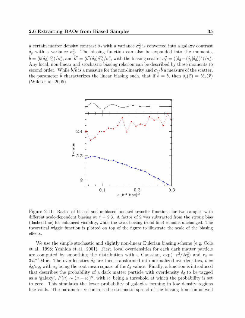
2.6 Extracting BAOs from Biased Samples 35
a certain matter density contrast δd with a variance σ2d is converted into a galaxy contrast
δg with a variance σ2g . The biasing function can also be expanded into the moments,
b = 〈b(δd) δ2d〉/σ2
d, and b2 = 〈b2(δd)δ2d〉/σ2
d, with the biasing scatter σ2b = 〈(δd−〈δg|δd〉)2〉/σ2
d.Any local, non-linear and stochastic biasing relation can be described by these moments tosecond order. While b/b is a measure for the non-linearity and σb/b a measure of the scatter,the parameter b characterizes the linear biasing such, that if b = b, then δg(~x) = bδd(~x)(Wild et al. 2005).
Figure 2.11: Ratios of biased and unbiased boosted transfer functions for two samples withdifferent scale-dependent biasing at z = 2.3. A factor of 2 was subtracted from the strong bias(dashed line) for enhanced visibility, while the weak biasing (solid line) remains unchanged. Thetheoretical wiggle function is plotted on top of the figure to illustrate the scale of the biasingeffects.
We use the simple stochastic and slightly non-linear Eulerian biasing scheme (e.g. Coleet al., 1998; Yoshida et al., 2001). First, local overdensities for each dark matter particleare computed by smoothing the distribution with a Gaussian, exp(−r2/2r2
0) and r0 =3h−1 Mpc. The overdensities δd are then transformed into normalized overdensities, ν =δd/σd, with σd being the root mean square of the δd-values. Finally, a function is introducedthat describes the probability of a dark matter particle with overdensity δd to be taggedas a ‘galaxy’, P (ν) ∼ (ν − νc)α, with νc being a threshold at which the probability is setto zero. This simulates the lower probability of galaxies forming in low density regionslike voids. The parameter α controls the stochastic spread of the biasing function as well

36 2. Probing Dark Energy with Baryonic Acoustic Oscillations
Figure 2.12: Boosted wiggle functions extracted with FITEX and theoretical wiggle functions forthe unbiased sample (filled circles and continuous line), for the strongly biased sample (trianglesand shot-dashed line) and for the less biased sample (open circles and long-dashed line). Thetheoretical wiggle functions are multiplied by the b-moment of the biasing function.
as its non-linearity. A value of α = 0.2 is a good compromise between reasonable non-linearity and a comparably tight spread. Two samples with νc = −0.2 and 0.6 weregenerated. Both parameters, α and νc, were adjusted to model the biasing parameters andnumber densities found by observation. SUBARU data (Hamana et al., 2004) suggests acomoving LAE density of n = 0.00301 ± 0.00194h3 Mpc−3 and a biasing parameter ofb = 4-5 at a redshift z = 5, which should decrease slightly with redshift. As discussedin Sect. 2.4 the biasing function b(δd) should translate into a boost of the power spectrumb2(k, z). Because the average slope of the biasing function is b, to first order we expectPbias(k) = P (k)b2(k, z) ∼ P (k)b2(z).
The two prescriptions lead to a biasing that either decreases or increases with k (seeFig. 2.11). Both values are consistent with the calculated b parameter. The comparativelystrong scale dependence of the biasing becomes evident when the ratios of the boostedtransfer functions are compared with the ratio of the wiggle amplitude to the transferfunction plotted on top of Fig. 2.11.
Figure 2.12 illustrates, that FITEX extracts BAOs even from biased galaxy distribu-tions. Plotted are the wiggle functions of the less strongly biased sample (open circles),the more strongly biased sample (open triangles) and the unbiased sample (filled circles)

2.7 Cosmological Tests with BAOs 37
at z = 2.3. The unbiased and biased oscillations vary because of shot noise, as the biasedsamples have a 2 and 10 times lower point density, respectively. Superimposed are thetheoretical wiggle functions (Eq. 2.1), normalized to the unbiased wiggle function (contin-uous line) and multiplied by the first moment of the biasing, b (dashed lines). The boostof the power spectrum obviously translates into an amplitude boost of the BAOs. As inredshift space, only the phenomenological fitting function as used in FITEX extracts theBAOs with a zero baseline, unlike when using a linear theory power spectrum.
However, not only the overall boost of the power spectrum, but also the k-dependencyof the biasing function should directly affect the amplitude of the BAOs. We tried to verifythis by fitting the Tw(k) function supplemented by a ‘linear biasing model’ to describe theextracted wiggle function Tex(k) = (a0 + a1 k)Tw(k). We notice that both parametersa0 and a1 are highly degenerate, mainly due to the fact that only data points at theextrema of the wiggle function significantly contribute to the fit. Data points at or nearthe nodes of the wiggle function are very insensitive to changes of the amplitude. Dueto the degeneracy, any amplitude a0 can easily be compensated by an appropriate valueof the parameter a1. Though the full fits had the expected slopes, the effects were verysmall and of no significance for the cosmological test. We may thus conclude that in acosmological test, which is mostly about detecting phase-shifts, it seems to be enough tofit the theoretical wiggle function with only an amplitude parameter, when the k-dependentbiasing is as weak as simulated here. However, more realistic simulations are needed toanalyze higher order effects.
2.7 Cosmological Tests with BAOs
The cosmological test compares the phases of the extracted BAOs with the theoretical wig-gle function, projected onto the hypersphere of the observer. As the theoretical templatedoes not model the amplitude of the oscillations with high accuracy, we are not able toinclude amplitude effects in the cosmological test and marginalize over the wiggle ampli-tude. Future tests should include this parameter, which is sensitive to w by e.g. structuregrowth.
A general feature of the test is that one first has to assume a certain reference cos-mology to get the metric scale of the wiggle function from the data, and to perform ina second step the comparison of the metric scale of the theoretical wiggle function rela-tive to the chosen reference cosmology (Glazebrook & Blake, 2005). In the present paper,we are interested in the performance of the BAOs extracted with FITEX in constrainingthe redshift-independent part of the w parameter of the dark energy. The amplitude ofthe theoretical function is also fitted but later marginalized. The remaining cosmologicalparameters are fixed to their values given at the end of Sect. 2.1.
As metric scales, comoving distances of the BAOs parallel and perpendicular to the LOSare used. Recall that in the plane-parallel or distant observer approximation, comovingdistances between two points with the same angular positions but different redshifts arex‖ =
∫ z2z1
dxdzdz = c
H0
∫ z2z1
dzE(z)
, where H(z) = H0E(z) is the Hubble parameter at redshift z

38 2. Probing Dark Energy with Baryonic Acoustic Oscillations
and E(z) the w-dependent transformation of the Hubble constant, H0, from redshift zeroto z (e.g. Peebles, 1993). To compute not distances between two points in space withdifferent redshifts, but parallel scaling factors between the two sets of cosmologies denotedby primed and unprimed symbols, one has to take the limit ∆z = z2−z1 → 0, which yields
x′‖ = x‖dx′
dx. (2.13)
Comoving perpendicular separations represent distances two points with the same redshiftbut different angular positions are separated, x⊥ = θ
∫ z20
dxdzdz, where θ is the angle be-
tween the two points. The scaling relation for the perpendicular component between twocosmologies thus becomes
x′⊥ = x⊥x′
x. (2.14)
In Fig. 2.13 the transformation ratio of the wiggle function is plotted at different red-shifts for two cosmologies that differ from the reference model only in w0 (the redshift-independent part of w). The reference model is the concordance cosmology. Fig. 2.13shows that the largest deviations from the reference model appear at redshifts in the range0.5 < z < 1.5. Differences in parallel and perpendicular scaling introduce anisotropies thatcould be measured, too (see below).
Figure 2.13: Transformation of perpendicular (solid) and parallel (dashed) distances in compar-ison to the concordance model with w0 = −0.7 (upper part) and w0 = −1.3 (lower part).
Figure 2.14 shows the scaled wiggle function at redshift z = 2.5 for w0 = −0.7. Thereference and the distorted wiggle function are plotted. Note that an elongation of thecoordinates in real space leads to a compression of the coordinates in k-space and viceversa. In the upper panel, it can be seen that the wiggle function gets more and moreout of phase as k increases. Thus the sensitivity of a cosmological test should increase athigh values of k. However, the amplitudes of the oscillations decrease exponentially withk (e.g., Silk damping). This can be seen in the lower panel of Fig. 2.14 where the scaledwiggle function is subtracted from the reference (w0 = −1) wiggle function: Though the

2.7 Cosmological Tests with BAOs 39
Figure 2.14: Scaled wiggle functions at z = 2.5 for w0 = −0.7 (dashed line) compared to thew0 = −1 cosmology (solid line, top panel). The normalized modulus of the difference betweenthe reference cosmology and the scaled cosmology is shown in the bottom panel. The dashedvertical lines mark the region relevant for the cosmological test.
difference in phase is increasing, the amplitude decreases so fast that the difference betweenthe projected oscillations increases at small values of k and decreases at high values of k.
The present version of the cosmological test comprises the following steps: (1) Angularand redshift coordinates of the ‘observed’ (simulated) data are transformed into comov-ing coordinates using a concordance model as the reference cosmology. (2) The comovingdata sample is Fourier-transformed to estimate the boosted transfer functions. (3) BAOsare extracted with FITEX. (4) The theoretical wiggle function is computed for the corre-sponding cosmological model. (5) The parallel and perpendicular scaling factors betweenthe test cosmology and the reference cosmology are computed at the redshift of the datasample. (6) The theoretical wiggle function is scaled by constructing a three-dimensionalwiggle function, scaling each mode and collapsing it to one dimension. (7) The observedwiggle function is compared to the re-scaled theoretical wiggle function assuming Gaussianstatistical errors (χ2 test). Only the steps (4-7) have to be repeated to test a differentcosmology, allowing a fast test of various parameters.
Note that the three-dimensional wiggle function is only constructed to simulate theeffects of different parallel and perpendicular scaling factors. It does not address theanisotropy introduced by redshift space effects, because we found that this only boosts

40 2. Probing Dark Energy with Baryonic Acoustic Oscillations
the various modes but not change the phases of the theoretical wiggle function (see Sect2.5). The boost effect of the redshift space distortions, along with other boosting effectslike biasing and growth suppression, will force us to add an additional parameter to thecosmological test.
Figure 2.15 shows in the upper left panel the combined wiggle function of the four XWwedge cubes of the Hubble Volume Simulation. The combination is performed by averagingover k-bins of discrete size. The errors represent the standard deviation of all wiggle pointsin the corresponding k-bins. After averaging, the 2nd to 5th BAOs are now clearly visible.We thus conclude that a volume at least 4 times larger than SDSS has to be sampledin order to see the BAOs with FITEX with high significance. One has to keep in mind,though, that our cubes are located at much higher redshifts, where the smoothing effectof non-linear structure growth is obviously much smaller. We also neglected the fact, thatlarger sky coverages reduce the sizes of the fundamental modes, leading to higher (better)sampling rates of BAOs.
With the 100 square degree sample, the possibility of data points appearing at positionswhich severely inhibit the accuracy of the cosmological test is relatively high, due to thehigh sample variance. Especially as only a few data points, which are far away frompositions where theoretical wiggle functions of different cosmological models intersect, havegreat statistical weight in the cosmological test. This fact is shown in Fig. 2.14, wherethe modulus of the difference between the theoretical transfer functions for two modelsdepending on position in k-space is plotted.
Figure 2.16 shows the results of the cosmological test obtained with BAOs extractedwith FITEX under different survey conditions. For surveys covering 100 square degrees wewould expect errors of σw0 = 0.25. The asymmetry of the error distributions directly reflectsthe increased sensitivity of metric scales on w for w0 > −1 compared to w0 < −1. At thesew0 values, the theoretical wiggle function gets quite compressed, so that at large k valuesthe amplitude decreases rapidly due to Silk damping. When w0 → −∞, the theoreticalwiggle function formally mimics the case of zero amplitude, so that low values of w0 areexcluded with about the same significance as the “no-wiggle” case of zero amplitude. Theminima of all error distributions plotted in Fig. 2.16 are slightly off-set from the inputw0 = −1 value, but well within all formal 1σ ranges.
Note that the constraints given above are based solely on the phases of the oscillationsin the one-dimensional power spectrum, assuming perfect knowledge of the sound horizonat drag epoch. The w-constraints are expected to further improve when the full twodimensional redshift space effects as well as the amplitudes of the BAOs are used.
Perhaps the most important result of the present investigation is the comparativelysmall decrease of only 8% of σw0 when comparing the w test with unbiased matter distri-butions in configuration space, (dashed line in Fig. 2.16) i.e., the simplest survey condition,with the test that includes all aforementioned effects (solid line). The robustness of theFITEX method to extract BAOs from boosted transfer functions with phenomenologicalfitting functions is mainly related to the fact that only the amplitudes of the wiggle func-tions are boosted by redshift-space and biasing effects, but the phases are not affected.

2.7 Cosmological Tests with BAOs 41
Figure 2.15: Combined wiggle functions from the four Hubble Volume cubes. The upper leftpanel shows the combined data point (dots) with self-consistent error bars for the 100 squaredegree field. The upper right panel shows expected error bars for 200 square degrees and thelower row with error bars for 300 and 600 square degrees, respectively. The continuous lines arethe theoretical wiggle functions for the reference (concordance) cosmology.

42 2. Probing Dark Energy with Baryonic Acoustic Oscillations
Figure 2.16: χ2 distributions for the w0 parameter obtained after marginalization over theamplitude parameter and for different conditions of BAO extraction. Short-dashed line: darkmatter distribution in configuration space over 100 sq. deg obtained from the simulation of darkmatter particles in configuration space. Continuous line: biased particle distribution in redshiftspace over 100 sq. deg. Dotted line: biased particle distribution in redshift space over 300 sq. deg(extrapolation). Dashed-dotted line: biased particle distribution in redshift space over 600 sq. deg(extrapolation). The horizontal dashed line marks the 1σ error level.
To give an idea of the performance of FITEX based on surveys of larger size, weextrapolated the results from the 100 square degree data. The upper right panel of Fig. 2.15shows wiggle functions extracted from the 100 square degree data but with error barsexpected for 200 - 600 square degrees. The error bars were extrapolated by scaling themaccording to the expected number of additional k-modes. The different survey fields arethus assumed to be not adjacent.
Figure 2.15 shows that increasing the survey volume to 200 square degrees does notreduce the error bars significantly, still allowing for crucial data points at peaks of theoscillating wiggle function to be reduced to zero amplitude. Error bars are still of the sameorder of magnitude as the oscillations. Only at 300 square degrees (lower left panel), theprobability for smoothing out the oscillations due to statistical errors gets considerably low.Following our extrapolations, for a survey of 600 square degrees, the errors are expectedto get much smaller than the amplitude of the oscillations and the chance of statisticaldeviations from the predicted function is of an order of magnitude that allows for veryaccurate cosmological probing.
The accuracies of the w0 parameter (Fig.2.16) range from σw0 = 0.25 for 100 sq. degwhich corresponds to 3 SDSS volumes, to σw0 = 0.09 for 600 sq. deg, corresponding to 21

2.8 Discussion and Conclusions 43
SDSS volumes. These results are obtained for biased samples in redshift space, i.e., themost complex survey condition. The improvement is directly related to the larger numberof independent k-modes in larger survey volumes and is consistent with results obtainedwith Monte-Carlo simulations (Blake & Glazebrook, 2003).
Future studies should also investigate the various parameters of the cosmological testto get constraints under less strong priors.
2.8 Discussion and Conclusions
We have seen that it is critical for the extraction of BAOs to either fit a phenomenologicalfunction to the continuum of the boosted transfer function (FITEX), or to calculate theshape of the boosted transfer function, including all distortions down to the sub-percentlevel. The latter approach has been carried out recently. Glazebrook & Blake (2005),Hutsi (2006), and Springel et al. (2005) used a linear theory power spectrum and dividedthe ‘observed’ data by this reference. Almost the same approach, but with the additionof linearizing the observational data before the division, to correct for non-linear structuregrowth was used in Angulo et al. (2005). There are two drawbacks of this method:
First, the ratio of a complex power spectrum and a reference power spectrum does notresemble a wiggle function as defined in the text, but something more complicated (seeEq. 2.4). The simple form of the theoretical wiggle function (Eq. 2.1) is strongly deformedby both the chosen transfer function of the reference spectrum and the distortions intro-duced by redshift space and galaxy biasing. These distortions make the comparison withtheoretically expected model spectra unnecessarily complicated. FITEX transforms theobserved power spectrum into a boosted transfer function where the subtraction of a non-oscillating phenomenological continuum function is directly related to Tw(k), multiplied byan amplitude factor.
The second drawback is the linear theory power spectrum itself. By computing acorrect shape of the power spectrum, one has to rely strongly on assumptions about thenature of the dark matter and various other physical processes. The method is no morethe ‘assumption free’ approach that was intended. Furthermore, the calculation of theamplitude factor that includes all the distortions ranging from linear structure growth,non-linear structure growth to redshift space distortions and biasing is a problem. Thiscalculation has to be accurate to the sub-percent level, as the oscillations themselves makeup only ∼ 2% of the transfer function.
A more phenomenological approach was conducted by White (2005). He assumedthat redshift space distortions as well as linear and non-linear structure growth could becalculated with reasonable accuracy. Leaving only the ratio between dark matter powerspectra and ‘galaxy’ power spectra, he found that one can fit this ratio with about 2%accuracy using a cubic polynomial. This adds further evidence that a phenomenologicalapproach can model power spectrum distortions without assuming much about the physicsof the distortions themselves.
With the FITEX method, we have shown that one is able to extract the BAOs without

44 2. Probing Dark Energy with Baryonic Acoustic Oscillations
any strong priors on the nature of dark matter or the shape of the power spectrum from thecomplex multi-component transfer function. All the aforementioned effects are modeled bythe continuum function and need not be known very accurately, as long as the phases of theoscillations are not distorted or washed out. This extraction is accurate on the sub-percentlevel within k-ranges relevant for the cosmological test. Furthermore, FITDEX is able todisentangle phase information from amplitude information which could in the future beused to test the geometry of the Universe on the one hand and the growth history on theother hand. This type of cosmological test could be used to discriminate Dark Energy fromModified Gravity theories.
We thank Ralf Bender for initiating this work on baryonic acoustic oscillations, theHETDEX team, the Virgo Consortium for the provision of the data of the Hubble Vol-ume Simulation, Urs Seljak and Mathias Zaldarriga for the CMBfast software, and DanielEisenstein and Wayne Hu for the software to compute transfer functions for high baryonfractions.

Chapter 3
The Impact of Sparse Sampling onPower Spectrum Cosmology
Note: this chapter will be submitted as Koehler et al. 2009. The work was performed underthe supervision of Niv Drory and with comments and suggestions by Eiichiro Komatsu.
3.1 Introduction
In the past, Blake et al. (2006) investigated the effect of sparse sampling on the ability torecover Baryonic Acoustic Oscillations (BAOs) in the galaxy power spectrum. They alsosimulated its impact on a cosmological test to constrain cosmological parameters like theequation of state of dark energy w. Sparse sampling introduces correlations between thedifferent Fourier modes (see Blake et al., 2006) and washes out the oscillations reducingtheir amplitude and thus their detectability. By using the full shape of the of the powerspectrum, one is less prone to effects of correlations, but has to model the spectrum veryaccurately including non-linear growth and scale dependent biasing to the percent level.Recently, Jeong & Komatsu (2006) and Jeong & Komatsu (2008) have shown that it is pos-sible to calculate these effects accurately at higher redshifts, using third order perturbationtheory and exploiting information from the bi-spectrum.
Cosmic variance describes the error of a sub sample representing the statistical proper-ties of the related super sample. The bigger the volume of a survey, the bigger the fractionof the universe covered and the smaller the cosmic variance. Cosmic variance affects mostlysmaller k modes, as increasingly more k modes of larger value fit into a given volume. Shotnoise describes the error of a sample with a finite point density representing the propertiesof an underlying continuous density field. The higher the point density the smaller thefluctuations in the density can be that can be accurately modeled. Shot noise affects mostlylarger k modes, as a higher point density is needed to model smaller scales correctly.
To increase survey volume and thus minimize error from cosmic variance, sparse sam-pling surveys do not sample the sky continuously, but leave large gaps between measure-ments, to trade volume for point density. The related window functions heavily distort the

46 3. The Impact of Sparse Sampling on Power Spectrum Cosmology
resulting power spectrum and introduce correlations both in the power itself and its error.
The upcoming Hobby-Eberly-Telescope Dark Energy eXperiment (HETDEX) (Hillet al., 2008) survey is utilizing Integral Field Spectroscopy Units (IFUs) and applies sparsesampling techniques (see Kaiser, 1986; Colombi et al., 1998) to search for Lyman AlphaEmitters (LAEs) as tracers for the underlying matter density field of the universe. Thepower spectra derived from this matter field can be used to test cosmological models, ex-ploiting the impact of cosmological parameters like the equation of state of dark energyw on the shape of the power spectrum. The ability to constrain cosmological parametersdepends on the relative accuracy of the measurement σ(k), which is dominated by the twosources of errors: Cosmic variance and shot noise. The shot noise depends on the powerin the sample P (k) and the average point density n, while cosmic variance depends on thesize of the survey L:
σ(k) =
√2π
k L
[1 +
1
n P (k)
]. (3.1)
In the present work, we will investigate the impact of such a window function on theresults of a cosmological test utilizing the full shape of the power spectrum. We will usea set of simulations described in Sect. 3.2 to directly test the impact of the proposedHETDEX IFU selection functions as well as additional zero-point effects (Sect. 3.3) on thepower spectrum. Section 3.4 will investigate the effect on the errors of the power spectrum,the error correlation matrix, and show how and to what extent one is able to correct forthe distortions. Finally we will show how the introduced additional errors and correlationsare affecting the accuracy of a cosmological test exploiting both geometrical and growtheffects of cosmological parameters in Sect. 3.5.
3.2 The Simulations
To test the various effects of different selection functions on the power spectrum and its er-rors we simulate 400 cubes with a baseline of 500h−1 Mpc and a total volume of 50h−1 Gpcusing the Pinocchio (PINpointing Orbit-Crossing Collapsed Hierarchical Objects) semi an-alytical method (see Monaco et al., 2002). The Pinocchio algorithm uses a numericalrepresentation of a linear density field to emulate non-linear structure growth by groupingparticles into halos, simulating the effects of accretion and mergers during the procedure.It calculates positions, velocities, merger history, and angular momentum of dark matterhalos, where positions are accurate to 2 Mpc and velocities to about 100 km s−1. We usethe power spectrum generated with the fitting function of Eisenstein & Hu (1998) as initialcondition.
Table 3.1 gives additional parameters of the simulations. The maximum and minimumk-values accessible to the simulation are given by the scale length of 500h−1 Mpc, andthe Nyquist frequency k = 1.61hMpc−1 of the simulations which equals 3.9h−1 Mpc,respectively. However, surveys with a baseline of smaller than 2h−1 Gpc or which are

3.3 Selection Functions 47
Table 3.1: Pinocchio ParametersPar Value DescriptionLgrid 256 grid size in 1 dimension
n 1.3e6 initial particlesΩΛ 0.75 dark energy densityΩm 0.25 matter densityΩb 0.045 baryon densityH100 0.72 normalized Hubble constantL 500 cube length in h−1 Mpcz 2.00 final redshiftσ8 0.8 power normalization
highly elongated do not gain a relevant amount of information from scales larger than500h−1 Mpc, and are thus also covered by the scale of the simulations used in this work.
Further testing suggest that the simulations should only be trusted to about 0.5hMpc−1
which equals a scale length of 12.6h−1 Mpc. This is mostly because of rapid power lossat larger k values due to the initial conditions of the simulations, where the particles arearranged on a regular grid. Similar effects can be found in other numerical simulations likethe Hubble Volume Simulation (see Koehler et al., 2007), where an initial glass distributiondistorts low k modes at high redshift.
The final redshift-space power spectrum averaged over all the 400 cubes is illustratedin Fig. 3.1. One can clearly see the power decay at higher values of k, where it deviatesfrom the linear prediction. The given error bars are calculated from the variance of thefull set of simulations and represent the errors of only one cube and agree very well withpredictions (see Subsect. 3.4.2). The errors of the mean power spectrum itself are smallerby a factor of
√400.
3.3 Selection Functions
Various selection functions work on the power spectrum to produce the final power ob-served.
The proposed HETDEX survey will utilize 96 IFUs, arrayed on a regular grid. TheIFUs themselves have a fill factor of only 1/3rd, but a dithering pattern will ensure acomplete sampling on the area of one IFU. This setup introduces, along with the radialselection function of a luminosity limited survey, a unique angular selection function.
We start looking at the radial selection function, which is dominated by the luminosityfunction of the LAEs and the thoughput of the telescope and instrument. Then, we willinvestigate the angular window function, dominated by the field of view of the IFUs andtheir fill factor of about 1/6th. And finally we will look at, zero-point offsets in theluminosity calibration that introduce correlations between nights, weeks and months, bysystematically over or under estimating the true matter density in one night, week, or

48 3. The Impact of Sparse Sampling on Power Spectrum Cosmology
0.1
1
10
100
1000
10000
100000
0.01 0.1 1
P(k
) [M
pc h
-1]3
k [Mpc-1 h]
Mean Power Spectrum
Figure 3.1: Mean power spectrum of 400 cubes with error bars of one cube calculated from thevariance within the whole sample.
month.
3.3.1 Radial Window Function
As HETDEX is a flux limited survey, the luminosity function and the distance to the objectdominate the radial selection function. However, because HETDEX utilizes IFUs to takespectra of every position on the sampled sky, the instruments throughput depending onwavelength and the sky spectrum also introduce selection effects in the radial direction.While the luminosity distance and instrument throughput are smooth functions of thedistance to, and thus wavelength of, the LAE, the sky spectrum is not smooth at all andcould potentially introduce strong correlations in the resulting power spectrum.
Figure 3.2 shows the radial selection function. It is calculated by multiplying thethroughput with the object density depending on distance and dividing by the sky spec-trum, as sky lines decrease the probability of finding a LAE at the related wavelength.
As the Pinocchio simulations only model dark matter halos and not galaxies, we simplyapply the radial selection function by selecting each halo according to a probability givenby the relative throughput of the selection function. This procedure neglects the fact thatLAEs with higher luminosities might or might not have a higher biasing than LAEs withlower luminosities. However, this topic is not yet well investigated, and the effect is mostlya change in slope and amplitude of the biasing. For a cosmological test the biasing has to

3.3 Selection Functions 49
0.3
0.4
0.5
0.6
0.7
0.8
0.9
1
3800 4000 4200 4400 4600 4800 5000
rela
tive
thro
ughp
ut
x [Mpc h-1]
Radial Selection Function
z-selectionsimulated cubes
Figure 3.2: Predicted fraction of LAEs detected at a certain distance normalized to the maximumdensity. Vertical lines contain the region used for the simulations.
be calculated using the higher order statistics of the bi-spectrum as suggested in Jeong &Komatsu (2008). In this work, we assume that biasing was determined using the suggestedmethods to a maximum k value of 0.3hMpc−1.
3.3.2 Angular Window Function
The proposed HETDEX selection function in angular dimension is heavily dominated bythe setup of fiberheads in the Visible Integral-field Replicable Unit Spectrograph (VIRUS).VIRUS covers only a small fraction of the telescopes field of view. The ratio of coveredarea, and thus volume, to uncovered area and volume, the fill factor, is only about 1/6th.This allows HETDEX to find an optimal balance between the cosmic variance error thatis dominated by the covered volume, and the shot noise error, which is dominated by thenumber of observed LAEs (see Eqn. 3.1).
As the IFU mask completely masks out a majority of the sky in angular direction, theresulting window function is conceptually different from angular selection functions of otherlarge surveys where power spectra are estimated like the SDSS (Tegmark et al., 2006) or2dF (Cole et al., 2005). In these surveys areas can be weighted according to their particledensity to compensate for selection effects like extinction or luminosity limitations. In thecase of HETDEX, the appropriate weight for a region with a points density of 0 would beinfinity and can not be corrected for or weighted. The information in the masked out area

50 3. The Impact of Sparse Sampling on Power Spectrum Cosmology
-4000
-2000
0
2000
4000
-4000 -2000 0 2000 4000
y [a
rcse
c]
x [arcsec]
Angular Selection Function
Figure 3.3: Angular selection functions displaying one shot of VIRUS (big squares) and the 96fiber-heads in each shot (small squares). The figure shows only a small part of the whole survey.
is lost.
Figure 3.3 illustrates the IFU selection function on they sky in angular coordinates. Itshows only a small part of the 400 degree survey area. A number of shots containing the 96fiber-heads are arranged in a static and very regular pattern in one shot. Our simulationsshow, that it is not necessary to arrange the IFUs in a shot randomly or even randomizethe IFU setting from shot to shot (see below), as the length scale of one IFU on the skyis only about 0.5h−1 Mpc, while the scales HETDEX is working on are about 50h−1 Mpc.The static setup of the IFUs in the shots is broken by a large gap in the middle, with asize of two times two fiberheads. This gap is used for other instruments.
The shots themselves are arranged in a semi random way using Monte Carlo methods.Firstly the shots are distributed on a regular grid, with some gaps between the shots. Thenone shot is randomly selected and moved by a random small distance in a random direction.If the shot overlaps another shot, the new position is canceled, if there is no overlap (withina small allowance) the new position is accepted. This procedure is repeated until the peakin the resulting power spectrum on the scale of the shot-separation is washed out as muchas possible.
We use this technique to simulate the semi random shot distribution resulting from thedistribution of stars on the sky. HETDEX will want to cover as many foreground stars aspossible for calibration. To achieve this, the shots will be nudged just a little from theiroriginal position on a regular grid to cover an optimal number of stars within their 1/6th

3.3 Selection Functions 51
fill factor.
1e-05
1e-04
0.001
0.01
0.1
1
0 0.005 0.01 0.015 0.02
w2 (k
)
k [arcsec-1]
Angular Window function
Semi-random SetupStatic Setup
Random SetupRandom Random Setup
Figure 3.4: The angular window function of a selection based on shots on a regular grid (longdashed line), a semi-random shot distribution (solid line), a random distribution (short dashedline), and a random shot, random IFU distribution (dotted line).
The difference between this semi-random shot setup and a complete regular grid is,however, not that big. Figure 3.4 shows the averaged 1-dimensional angular window func-tions of both setups. In the semi-random setup, the two dominant peaks from the gridsize itself at k = 5 × 10⁻³arcsec−1 and the harmonies at two and four times this value arewashed out in comparison to the regular grid. However, the semi-random window functionhas more power itself, than the static function, which will lead to a stronger distortion ofthe power spectrum in the end.
A completely random placement of the shots with an average distance D was alsoconsidered. This has the advantage of having a simple window function with a 1/D profile,where all other features are washed out and smoothed as much as possible (see Kaiser,1998). However, as D is comparable to scales of interest, the window function is verybroad and has a lot of power itself. Furthermore, the completely random placing leadsto heavy overlap, effectively decreasing the sampled volume by a considerable amount.Because of this, the completely random shot setup was dismissed.
Finally one can compare the completely random shot setup with IFUs placed on a staticgrid within a shot, and a setup where not only the shots are randomized, but also the IFUssetup within every shot. Figure 3.4 shows a difference on the scale of k = 0.01arcsecand higher where the correlations are dampened compared to the static IFU case. The

52 3. The Impact of Sparse Sampling on Power Spectrum Cosmology
difference is, however, not big enough to compensate for the effort to mechanically reshufflethe setup of the IFUs for every shot.
3.3.3 Luminosity Calibration
Not only the pattern of shots itself, but also the clustering of shots within one night oreven week or month might introduce correlations into the data. The shots of one HETDEXreference design night are clustered into two squares approximately 10 degrees apart. Ata redshift of two, this equals more than the maximum scale length 500h−1 Mpc of oursimulations. Thus, we only capture the effect introduced by the correlations of one cluster.
To simulate this effect, we randomly calculate the extinction in this night, based onreal data. We assume that luminosity zero-point is calculated correctly with a lognormalerror distribution
δzp(x) =1
σ√
2 πe−
(ln(x)−µ)2
2σ2 , (3.2)
normalized to a standard deviation of of 5% and 10% and a mode of 1. The lognormaldistribution is motivated by the experience from the VIRUS-P prototype survey (see Hillet al., 2008).
Each shot in a night shares the same zero-point error, which means that all the shots inone night are 100% correlated. The error in number counts is then computed by calculat-ing the difference in number density for the real extinction, and the errornous extinctiondepending on distance, and applying this ratio as a weight to all the detected LAEs in onenight.
We assume a three by three shot pattern for one of the two clusters a night, only oneof which will fall into our simulated volume. Correlations between weeks and months arenot considered in this work, as the nightly correlations will be much stronger and can thus,especially with a maximum correlation of 1, be used as an ideal test case to judge theimpact of correlations of other time scales and correlation strengths.
3.3.4 Cartesian Window Function
In spherical coordinates, both the angular as well as the radial correlation function areindependent of each other. However, a three dimensional power spectrum can not easilybe calculated using spherical coordinates, as the resulting power spectrum scales changefrom radial shell to radial shell and can not easily be added up to a cumulative or meanpower spectrum of the whole volume without washing out major features. Angular powerspectra in redshift slices are used to achieve this (see Blake et al., 2007), but throw awayinformation in form of the correlations between the slices. It was furthermore shown thatlightcone effects and the breaking of the distant observer relation in rectangular volumes ofabout 10h−1 Gpc and a redshift of 2 and more do not affect the calculated power spectrummuch (see Wagner et al., 2008).

3.3 Selection Functions 53
-100
-50
0
50
100
-100 -50 0 50 100
y [M
pc h
-1]
x [Mpc h-1]
Shot allignement at different Redshifts
Figure 3.5: Spatial distribution of shots on a regular grid at a distance of 3500h−1 Mpc (graysquares) and 4000h−1 Mpc (black squares).
We will thus investigate the impact of both the angular and radial selection functionsusing a Cartesian Fourier transform to calculate the power spectrum. The breaking of thedistant observer relation leads to a mixing of the formerly independent selection functionsand heavily distorts the angular pattern depending on the distance to the observer.
Figure 3.5 shows how an angular selection function with equally spaced shots in angularcoordinates would work on a sample of simulated LAEs in a distance of 3500 (blue) and4000h−1 Mpc (red). One can clearly see that any distinct scales, like the spacing of thevarious shots from each other, or the size of the shots themselves, are distorted with thedistance from the center of the cube, and the distance to the observer. Because of this,the power on any angular scale is washed out and distributed within the whole cube in theCartesian Fourier transform.
As a result, only the modes purely parallel to the line of sight carry the signal of thewashed out radial selection function and the modes purely transversal to the line of sightcarry the signal of the washed out angular selection function. Figure 3.6 shows a logarith-mic representation of the two dimensional window function, where the two perpendiculardimensions were integrated to one. Modes that comprise of both parallel and perpendicularparts have practically no power and resulting correlations are kept to a minimum.

54 3. The Impact of Sparse Sampling on Power Spectrum Cosmology
1e-07
1e-06
1e-05
1e-04
0.001
0.01
0.1
0 0.1
0.2 0.3
0.4 0.5
0.6 0.7
0.8
0 0.1
0.2 0.3
0.4 0.5
0.6 0.7
0.8
1e-08
1e-07
1e-06
1e-05
1e-04
0.001
0.01
0.1
1
w2(k)
2D Window function
LOS k [Mpc-1 h]perp k [Mpc-1 h]
w2(k)
Figure 3.6: Window function in both the parallel and perpendicular direction. Note the loga-rithmic scale in z.
3.3.5 Samples
By applying all the selection functions to the 400 simulation cubes, we end up with fivedifferent samples:
• an undistorted sample, including redshift-space effects and (semi-analytic) non-lineargrowth
• a sample including the above plus radial selection effects
• a sample including the above plus angular selection effects
• a sample including the above plus 5% zero-point errors
• a sample like the above but with 10% zero-point errors
All the samples were generated by projecting the angular and radial selection functionsto a Cartesian coordinate system, placing the cubes at a distance of 4000 to 4500h−1 Mpcfrom the observer at an average redshift of 2.5.

3.4 Error Analysis 55
A number of effects are not covered. They include, but are not limited to:
• lightcone effects (see Wagner et al., 2008)
• scale dependent biasing (see Jeong & Komatsu, 2008)
• luminosity dependent biasing (see Orsi et al., 2008)
• velocity dispersion effects of emitting medium (see Tapken et al., 2007)
All of them should, however, not affect the comparison of power spectra with differentwindow functions.
3.4 Error Analysis
This section will show the effects of the various selection functions on the power spectrumitself, the errors of the power spectrum, and the correlations of the errors.
3.4.1 Systematic Errors
All three window functions introduce distortions to the power spectrum. An initial over-density distribution δ(~x) is transformed by an arbitrary selection function n(~x) like,
δ(~x) = n(~x)δ(~x), (3.3)
with 0 ≤ ~k ≤ 1. The FKP algorithm (see Feldman et al., 1994) calculates overdensitiescorrectly by subtracting a homogeneous sample multiplied by the selection function fromthe inhomogeneous sample. The resulting estimated power spectrum after subtraction ofshot noise is then a convolution of the true power spectrum with the window function:
P (~k) = P (~k)⊗ |n(~k)|2 . (3.4)
The window function is given by
n(~k) =∫d3x n(~x) exp(i~k · ~x), (3.5)
the square of the Fourier transformed selection function. The power spectrum itself iscalculated using the FKP algorithm (see Feldman et al., 1994) using a grid with 256 gridpoints and a next grid point allocation algorithm (NGP). We do not correct for aliasingeffects, but it was shown by Jing (2005) that the lower k-modes are not affected by aliasing.
The ratios between the undistorted power spectrum and the z-selected and IFU-selectedpower spectra of the 400 cubes are plotted in the upper panel of Fig. 3.7. The lower panelshows the ratio between the IFU-selected power spectra and the 5% and 10% zero-pointerrors power spectra, respectively.

56 3. The Impact of Sparse Sampling on Power Spectrum Cosmology
0.01
0.04
0.16
0.64
0.1 0.2 0.3 0.4 0.5
Rat
io -
1
k [Mpc-1 h]
Power Spectra Ratios
z-selectionIFU-selection
0.005
0.025
0.125
0.625
0.1 0.2 0.3 0.4 0.5
Rat
io -
1
k [Mpc-1 h]
5% weather10% weather
Figure 3.7: Upper panel: z-selected (+) and IFU-selected (x) power spectra divided by theundistorted redshift-space power spectra.Lower panel: Power spectra from data with 5% zero-point errors (+) and 10% zero-point errors(x) divided by the IFU-selected power spectrum without zero-point effects.

3.4 Error Analysis 57
While the absolute change in amplitude due to the radial window function and thezero-point errors are relatively small, the angular window function heavily distorts theobserved power spectrum.
Another difference is the scale most affected by the distortions. Angular effects increaseat smaller scales, while zero-point effects decrease at smaller scales. This is expected, asthe angular window function is dominated by the relatively small scale of the shots, butmuch more by the scale of the IFUs fiberheads themselves which are, however, too small tobe resolved by the power spectra of our simulations. Zero-point effects on the other handare dominated by the much larger cluster scale of correlated shots in one night.
Correcting for Selection
To measure the impact of the distortions due to the window functions on a cosmologicaltest we have to calculate how accurately the initial power spectrum can be recovered fromthe observations, or how well a distorted template can be calculated.
As a convolution is much easier to calculate than a deconvolution we try to modelthe distorted power spectrum by convolving a theoretical model power spectrum by thewindow function. It is not necessary to do this convolution for all possible scale factors inthe following geometric test, as we are only probing for small variations from the referencecosmology. In this case, the linear expansion, and thus a simple re-scaling of the convolutedpower spectrum to the tested scale factor ( see Sect. 3.5) does suffice.
We compute the three dimensional window function numerically by applying the IFU-and z-selection functions on a high density random sample and compute the Fourier trans-form with fast Fourier transform algorithm (FFT).
Figure 3.8 shows the ratio between the convolutions with various degrees of resolutionsand the power spectrum including the radial and angular selection effects. We start with256 grid points per 500h−1 Mpc cube and increase to 512 and 1024 grid points. However weachieve this not by increasing the actual number of grid points but use the same numberof grid points on the full cube, a smaller sub-cube with half the length, and an againsmaller sub-cube with one fourth the base length. This distorts the lower k-scales of thehigher resolution spectra and only the high k-scales should be accurate. Furthermore,the different resolutions vary, because the smaller samples of the higher resolutions onlycapture a fraction of the overall, inhomogeneous, window function.
The convolution with the lowest resolution agrees well at low k-scales, which was ex-pected. The highest resolution agrees well with the power spectrum including the selectioneffects at higher k-scales, while it is loosing power on large scales. However, the error barsdue to different shot noise and sample variance are still of an order of 1% per data point,which is approximately the accuracy of a survey with 8h−3 Gpc3 volume and 10 milliontracer particles with a biasing of 2 at k = 0.2hMpc−1 and a redshift of 2. HETDEX isreaching an accuracy of about 2.5% at this k-value.
Thus, we can conclude that the issue of correcting for the window function has to beexamined further to exclude any systematic effects at an accuracy comparable to the sur-veys statistical error. The problem is not to calculate the window function to an arbitrary

58 3. The Impact of Sparse Sampling on Power Spectrum Cosmology
0.7
0.8
0.9
0.95
1
1.05
0 0.1 0.2 0.3 0.4 0.5
Rat
io -
1
k [Mpc-1 h]
Comparison of convolution ratios
undistortedsingle resolution
double resolutionquadrouble resolution
Figure 3.8: Ratio between the undistorted power spectrum (solid line), the single resolutionconvolution (long dashed line), double resolution convolution (short dashed line), quadruple res-olution convolution (dashed dotted line) and the IFU-selected power spectrum.
accuracy, but confirming the accuracy by carrying out the convolution.
Correcting for Zero-Point Uncertainties
Assuming a Gaussian zero-point error distribution with a variance of σ2zp and a window
function w(x) the overdensities δ(~x) with zero-point errors can be calculated like:
δ(~x) = n(~x) [δ(~x) + σww(~x) δ(~x)] . (3.6)
Because of the distributivity of convolution, we can express the power spectrum withzero-point effects and selection effects, P (k), by a sum of only the spectrum with selectioneffects, P (k), and an additional power term:
P (~k) = P (~k) + σ2w P (~k) ⊗
∣∣∣w(~k)∣∣∣2 , (3.7)
with w(k) being the Fourier transformed window function.The additional power term is proportional to the square of the error in the luminosity
calibration σzp.To test how well the relation holds in a simulated environment, we calculate the addi-
tional power by subtracting P (k) from P (k) with 5% zero-point errors. As the sigma-ratiobetween the 10% and 5% error case is 2, we multiply the additional term by 4 and add it

3.4 Error Analysis 59
0.005
0.025
0.125
0.625
0 0.1 0.2 0.3 0.4 0.5
(Pk
- P
k ref
)/P
k ref
k [Mpc-1 h]
Weather correction
5% weather5% weather x 4
10% weather
Figure 3.9: Ratio between the power spectrum with 5% zero-point errors (+), the 10% zero-pointerrors (*) and the IFU-selected power spectrum. The crosses with errorbars show the 5% datacorrected in amplitude to match the 10% data.
to P (k). The result should match the 10% error case. Figure 3.9 shows the excellent agree-ment of the original 10% zero-point error power spectrum and the model. The agreementis better than the random errors of the 400 cubes. These are not affecting this comparison,as both the 5% and 10% case share the same error in the initial power spectrum, due tocosmic variance and shot noise, but not in the statistically independent zero-point errors.
As the correction is better than the statistical error of the initial power spectrum, theimpact of the zero-point effects can be corrected for and thus neglected in the cosmologicaltest as long as the shape of the error distribution is well known. While a different shapeis changing the form of the additional power term, the integral, measured to first order byσw, is proportional to the amplitude of the additional term. In the case of HETDEX theerror of the luminosity calibration should be known to about 1%.
3.4.2 Statistical Errors
Using simple mode counting arguments, the relative error of a power spectrum σP (k) isgiven by Eqn. 3.1.
Additional errors are introduced by mode coupling and mixing due to redshift and non-linear growth effects. Both of them are, to some extent, included in the semi-numericalsimulation. Note that, because of the high redshift range of HETDEX, these errors arevery small. More errors are introduced via correlations with the window functions and

60 3. The Impact of Sparse Sampling on Power Spectrum Cosmology
zero-point effects. In this section, we will investigate the impact of the various selectioneffects on the absolute error.
The error of the error can be calculated as,
Stddev(σ) = σ1√2N
. (3.8)
With N = 400 cubes, this results in a relative error accuracy of 3.5% per data point,or a cumulative 0.4% for all 40 data points of one power spectrum to a maximum k valueof 0.3hMpc−1
0.02
0.1
0.5
0 0.1 0.2 0.3 0.4 0.5
Rel
ativ
e E
rror
k [Mpc-1 h]
Undistorted
measured errorscalculated errors
0.02
0.1
0.5
0 0.1 0.2 0.3 0.4 0.5
Rel
ativ
e E
rror
k [Mpc-1 h]
z-selection
measured errorscalculated errors
0.1
0.5
0 0.1 0.2 0.3 0.4 0.5
Rel
ativ
e E
rror
k [Mpc-1 h]
IFU-selection
measured errorscalculated errors
0.1
0.5
0 0.1 0.2 0.3 0.4 0.5
Rel
ativ
e E
rror
k [Mpc-1 h]
10% weather
measured errorscalculated errors
Figure 3.10: Relative errors calculated from Eqn.3.1 (solid line) and estimated from the numericalsample (data points). The error bars are given by Eqn. 3.8. From left to right and bottom to top:Undistorted power spectra, z-selected power spectra, IFU-selected power spectra, power spectrawith 10% zero-point errors.
Figure 3.10 shows the errors computed using the statistical variance of the simulationsthemselves and the errors predicted by Eqn. 3.1. We plot the errors of the undistortedspectra in the lower right panel, and errors of a power spectrum with radial selectioneffects in the lower right panel. The upper left and right show spectra with additional

3.4 Error Analysis 61
angular selection effects and 10% zero-point effects, respectively. The absolute error ofthe simulations is increasing from left to right and bottom to top, because more and moreparticles are excluded due to selection and thus increase shotnoise errors.
Because of the high redshift of z = 2 of the simulations, redshift-space effects andnon-linear growth do not affect the error budget of the power spectrum much, and theundistorted redshift-space power spectrum matches the predictions perfectly, at least atscales relevant for HETDEX up to k = 0.3hMpc−1. The radial selection function also doesnot introduce considerable errors, while the angular selection function increases the errorsby a relative mean of 5%. The zero-point effects do not further alter the error budgetconsiderably.
For a cosmological test this means that a relative increase of the error by5% translatesdirectly into a decrease of accuracy by a relative 5%.
3.4.3 Correlation Matrix
The correlation matrix gives the correlation of a mode k with another mode k′, with thecase of total correlation normalized to 1 and total anticorrelation normalized to -1. Wecalculate the mean correlation matrix ρ(k, k′) by calculating the mean power 〈P (k)〉 andthe error σ(k) from the N = 400 cubes, compute the correlation matrix for one cube, andaverage over all the cubes i using
ρ(k, k′) =1
N
N∑i=1
(〈P (k)〉 − Pi(k)) (〈Pi(k′)〉 − P (k′))
σ(k)σ(k′). (3.9)
Figure 3.11 shows the correlation matrices of the various samples. Unfortunately theaccuracy of each element in the correlation matrix is, given Eqn. 3.8 and Gaussian errorpropagation, only 5%. Figure 3.11 clearly shows fluctuations on the order of 5%.
Within the error bars, the z-selection does not have a considerable effect on correlations.This was expected, as the selection in line of sight direction only affects one third of themodes, in contrast to two thirds for the angular selection function. The function itself isquite smooth with uncorrelated modulations due to the spectrum of the night sky whichmodulates the selection in z-direction. Further resolution effects of the instrument can beneglected as z-resolution scale is far smaller than any scale of interest. The angular windowfunction introduces noticeable correlations along all length scales. This agrees well with theassumption that the strong correlations form the angular window function are washed outin Cartesian space and distributed over all length scales. The correlations due to zero-pointeffects seem to increase rapidly with higher values of k. The main correlation length of thevolume covered in one night is 60h−1 Mpc which corresponds to a k value of 0.1hMpc−1.All scales smaller than this length should have the correlations from the angular windowenhanced, as the zero-point distortions are working on exactly that pattern.
The lower panel of Fig. 3.11 is zoomed in on the k values relevant for HETDEX. Here,the correlations are dominated by the IFU selection function, while the effect of both z-selection and zero-point effects is small. The increase in correlation due to IFU-selection

62 3. The Impact of Sparse Sampling on Power Spectrum Cosmology
-0.1 -0.05 0 0.05 0.1 0.15
Undistorted
0 0.2 0.4 0.6 0.8 1 1.2 1.4 1.6
k [Mpc-1 h]
0 0.2 0.4 0.6 0.8
1 1.2 1.4 1.6
k [M
pc-1
h]
-0.1 -0.05 0 0.05 0.1 0.15
z-selection
0 0.2 0.4 0.6 0.8 1 1.2 1.4 1.6
k [Mpc-1 h]
0 0.2 0.4 0.6 0.8
1 1.2 1.4 1.6
k [M
pc-1
h]
-0.1 -0.05 0 0.05 0.1 0.15
IFU-selection
0 0.2 0.4 0.6 0.8 1 1.2 1.4 1.6
k [Mpc-1 h]
0 0.2 0.4 0.6 0.8
1 1.2 1.4 1.6
k [M
pc-1
h]
-0.1 -0.05 0 0.05 0.1 0.15
10% weather
0 0.2 0.4 0.6 0.8 1 1.2 1.4 1.6
k [Mpc-1 h]
0 0.2 0.4 0.6 0.8
1 1.2 1.4 1.6
k [M
pc-1
h]
-0.1 -0.05 0 0.05 0.1 0.15
Undistorted
0 0.1 0.2 0.3 0.4 0.5
k [Mpc-1 h]
0
0.1
0.2
0.3
0.4
0.5
k [M
pc-1
h]
-0.1 -0.05 0 0.05 0.1 0.15
z-selection
0 0.1 0.2 0.3 0.4 0.5
k [Mpc-1 h]
0
0.1
0.2
0.3
0.4
0.5
k [M
pc-1
h]
-0.1 -0.05 0 0.05 0.1 0.15
IFU-selection
0 0.1 0.2 0.3 0.4 0.5
k [Mpc-1 h]
0
0.1
0.2
0.3
0.4
0.5
k [M
pc-1
h]
-0.1 -0.05 0 0.05 0.1 0.15
10% weather
0 0.1 0.2 0.3 0.4 0.5
k [Mpc-1 h]
0
0.1
0.2
0.3
0.4
0.5
k [M
pc-1
h]
Figure 3.11: Upper Panel: Correlation matrices of, from left to right and bottom to top,undistorted power spectra, z-selected power spectra, IFU-selected power spectra, and powerspectra with 10% zero-point errors.Lower Panel: Same correlation matrices, but zoomed in on the region relevant for HETDEX.

3.5 Cosmological Test 63
at these scale seems to, at least with the resolution provided by the 400 cubes, affect allscales uniformly with a mean increase in correlation to about 0.04.
3.5 Cosmological Test
A wide variety of dark energy models are currently proposed (see Copeland et al., 2006)with various parametrization of the equation of state of dark energy, w, and its behaviorin time. Models include, but are not limited to, standard dark energy (Carroll et al.,2003), brane world models (Sahni & Shtanov, 2003), or quintessence (Caldwell & Linder,2005). Because the time dependent as well as the time independent characteristics of ware affecting the power spectrum as a function of redshift, we do not test for w directly,but only calculate the impact on geometry and growth. Given a certain dark energy modelone can then convert these results to accuracies on w and its various parametrizations.
The effect of w on geometry is measured by calculating the goodness of fit from the dataand a reference cosmology scaled by a dimensional scale factor, s. The effect on growth iscalculated by computing the goodness of fit between the data and a reference cosmologywith an amplitude scaled by a growth ratio d.
3.5.1 Geometric Test
The geometric cosmological test is based on the fact that the distance of an object on thesky both in radial and in angular direction is a function of cosmological parameters, likethe dark energy density ΩΛ, the total matter density, Ωm, and the equation of state ofdark energy, w. Surveys only measure the redshift, z, and the angular separation, φ, ofobjects. The co-moving line of sight distance, x‖, and the co-moving angular distance, x⊥,are calculated from redshift and angular separation:
x‖ =∫ z2
z1
dx
dzdz , (3.10)
x⊥ = φ∫ z2
0
dx
dzdz , (3.11)
using the relation,
dx
dz=
c
H(z,ΩΛ,Ωm, w). (3.12)
with H(z) being the redshift dependent Hubble constant.In the case of a flat universe, the Hubble constant can be approximated as,
H(z) = H0
√Ωm (1 + z)3 + ΩΛ e
3∫ z0d ln(1+z′) [1+w(z′)] , (3.13)
with H0 being the Hubble constant measured today.

64 3. The Impact of Sparse Sampling on Power Spectrum Cosmology
To perform a geometric test, redshifts and angular separations have to be convertedinto into co-moving distances using a test cosmology. A power spectrum can then be cal-culated from the resulting positions and the result compared to a template power sectrumcalculated from theory using a reference cosmology.
As this is very time consuming, this process can, as shown in Koehler et al. (2007) beemulated by scaling only the resulting power spectrum. The ratio in scale length s is afunction of the ratios in parallel and perpendicular direction
s (ΩΛ,Ωm, w) =1
3
x‖x‖
+2
3
x⊥x⊥
, (3.14)
with x denoting the length scale of a test cosmology and x being the length scale ofthe reference cosmology. Although the parallel and perpendicular modes can not, dueto the braking of the distant observer relation, be directly translated into the Cartesiancoordinates of the Fourier transform, Wagner et al. (2008) has shown that the difference canbe neglected in HETDEX like surveys, where only a small fraction of the sky is sampled.
The power spectrum itself scales with the scale ratio s both in frequency and in ampli-tude
P (k, s) = s−3 P (k s) . (3.15)
As the power spectrum declines at higher k values like a power law with a slope of-1.8, the scaling relation is dominated by the decline in amplitude and not by the phasecontribution.
3.5.2 Growth Test
Cosmological parameters like w are also affecting linear structure growth, by delaying oramplifying the growth rate, and thus the amplitude of the power spectrum, independentlyfrom the geometrical effect. To measure both the geometrical part and the linear growthD, we include the ratio of structure growth factors
d (ΩΛ,Ωm, w) =D
D, (3.16)
where the reference growth factor D is determined by the reference cosmology and Dby the cosmological parameters of the test cosmology. D can be approximated (see Linder& Jenkins, 2003) like
D (ΩΛ,Ωm, w) =5
2ΩmH(z)
∫ a
0da [aH(z)]−3 , (3.17)
with the scale factor a ∝ (1 + z)−1. The power spectrum itself scales with the growthratio d only in amplitude
P (k, d) = d2 P (k) . (3.18)

3.5 Cosmological Test 65
In this case, the scaling relation is purely determined by amplitude.
3.5.3 Test Setup
Combining both the geometrical and growth scaling relations we end up comparing a testpower spectrum
P ∗(k, s, d) = d2 s−3 P (k s) , (3.19)
with the reference power spectrum P (k) depending on various cosmological parameters,including biasing b, structure growth D, matter and dark energy content Ωm,ΩΛ, and thenormalization σ8 in addition to some other parameters.
We use a simple χ2-test to calculate to goodness of fit between the reference and the testcosmology. The power spectral template is computed using CAMB (Lewis et al., 2000).
Table 3.2: CAMB ParametersPar Value Descriptionw -1 equation of state of DEΩΛ 0.75 dark energy densityΩm 0.25 matter densityΩb 0.045 baryon densityH100 0.72 normalized Hubble constantz 0.0 final redshiftσ8 0.79 power normalizationτ 0.087 optical depth
The errors and the effects of the various selection functions are estimated to first orderby computing the error σ(k) according to Eqn. 3.1 an multiplying them by the ratioof simulated to computed error given in Fig. 3.10 to include errors introduced by nonlinearities, redshift-space, and of course the selection functions. The covariance matrixcovij is calculated using covij = σi ρij σj.
The final χ2 test is then computed using:
χ2 = [P ∗(k)− P (k)]T cov−1(k, k′) [P ∗(k′)− P (k′)] . (3.20)
We only include the modes to a maximum k value kmax. It is suggested by Jeong& Komatsu (2006) that at redshift two, the maximum reliable wavelength is kmax =0.3, hMpc−1.
The test proceeds as follows:
• Calculate reference power spectrum
• Convolute reference power spectrum
• Chose test parameters s and d

66 3. The Impact of Sparse Sampling on Power Spectrum Cosmology
• Calculate test power spectrum
• Calculate errors of the test spectrum
• Simulate data with errors using Monte Carlo methods
• Calculate χ2 value
In our test we rescale the errors to match those of a survey with a volume of 2.7h−3 Gpc3
and 0.8 million particles at a redshift of 2.5 and a mean biasing of 2.5. For simplicity, andbecause we only want to differentially compare the impact of the selection function, weneglect the fact that the particle densities in a flux limited survey are distributed in-homogeneously and that biasing might change with redshift.
3.5.4 Results
Figure 3.12 shows the result of the cosmological test using the undistorted power spectrum.The two parameters d and s are highly degenerate. Fortunately the impact of w on thescale ratio s and the growth ratio d is, according to most sensible models (see Linder &Jenkins, 2003) correlated in their effect on the power spectrum. When w goes up, the scaleratio goes down, which leads to an increase of amplitude. A more positive w also leads toan increase in the growth ratio and thus an increase of amplitude.
The gray area in Fig. 3.12 illustrates what parameter combinations are allowed withcurrent models of dark energy. With s and d being antiproportional in most current modelsof dark energy, the resulting model curve in the s-d-plane with a negative slope breaks thedegeneracy of the test and leads to well constrained values.
To better show the effect of the selection functions on the test, we fix one parameterat 1, which actually underestimates the accuracy because of the anti correlation of theparameters given a model of dark energy, and vary the other. In Figure 3.13 the χ2 valuesfor the undistorted, the z-selected, the IFU-selected, and the 10% zero-point errors aregiven. In the top panel of the figure, the results for the scale parameters s are given,while the lower panel shows the results for the growth parameter d. The scale parameteris much better constrained than its counterpart in growth, as the power spectrum has aphase dependence on s and a stronger amplitude dependence than d.
While the impact of the z-selection on both parameters is barely visible, the IFU-selection decreases the accuracy of the test by a relative 16%. The 10% zero-point errorsdecrease the accuracy by 23% relative to the undistorted case.
To test whether the increase of absolute error, or the correlations introduced by theselection functions have the most impact on accuracy, we conduct two additional cosmo-logical tests:
• the best errors (undistorted) and the worst correlation matrix (10% zero-point errors)
• the worst errors (10% zero-point) and the best correlation matrix (undistorted)
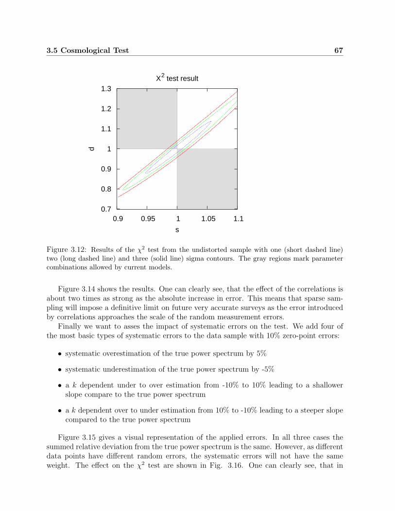
3.5 Cosmological Test 67
Χ2 test result
0.9 0.95 1 1.05 1.1
s
0.7
0.8
0.9
1
1.1
1.2
1.3d
Figure 3.12: Results of the χ2 test from the undistorted sample with one (short dashed line)two (long dashed line) and three (solid line) sigma contours. The gray regions mark parametercombinations allowed by current models.
Figure 3.14 shows the results. One can clearly see, that the effect of the correlations isabout two times as strong as the absolute increase in error. This means that sparse sam-pling will impose a definitive limit on future very accurate surveys as the error introducedby correlations approaches the scale of the random measurement errors.
Finally we want to asses the impact of systematic errors on the test. We add four ofthe most basic types of systematic errors to the data sample with 10% zero-point errors:
• systematic overestimation of the true power spectrum by 5%
• systematic underestimation of the true power spectrum by -5%
• a k dependent under to over estimation from -10% to 10% leading to a shallowerslope compare to the true power spectrum
• a k dependent over to under estimation from 10% to -10% leading to a steeper slopecompared to the true power spectrum
Figure 3.15 gives a visual representation of the applied errors. In all three cases thesummed relative deviation from the true power spectrum is the same. However, as differentdata points have different random errors, the systematic errors will not have the sameweight. The effect on the χ2 test are shown in Fig. 3.16. One can clearly see, that in

68 3. The Impact of Sparse Sampling on Power Spectrum Cosmology
0
5
10
15
20
0.97 0.98 0.99 1 1.01 1.02 1.03
∆ Χ
2
s
Χ2 tests with different spectra
undistortedz-selection
IFU-selection10% weather
0
5
10
15
20
0.925 0.95 0.975 1 1.025 1.05 1.075
∆ Χ
2
d
undistortedz-selection
IFU-selection10% weather
Figure 3.13: Results of the χ2 test with d parameter fixed at 1 (upper panel) and the s parameterfixed at 1 (lower panel). The solid line denotes the results of the undistorted sample, the longdashed line of the z-selected sample, the short dashed line of the IFU-selected sample, and thedash-dotted line of the sample with 10% zero-point effects. Horizontal dashed lines give the one,two, and three sigma levels for the goodness of fit.

3.5 Cosmological Test 69
0
5
10
15
20
0.97 0.98 0.99 1 1.01 1.02 1.03
∆ Χ
2
s
Χ2 tests with different spectra
undistortedhigh error, low correlationlow error, high correlation
0
5
10
15
20
0.925 0.95 0.975 1 1.025 1.05 1.075
∆ Χ
2
d
undistortedhigh error, low correlationlow error, high correlation
Figure 3.14: Results of the χ2 test with d parameter fixed at 1 (upper panel) and the s parameterfixed at 1 (lower panel). The solid line shows the results of the undistorted sample, the long dashedline of a test using the worst error of all samples and the best correlation matrix, the short dashedline gives the results for the best errors and worst correlation matrix. Horizontal dashed linesdenote the one, two, and three sigma levels for the goodness of fit.

70 3. The Impact of Sparse Sampling on Power Spectrum Cosmology
-0.15
-0.1
-0.05
0
0.05
0.1
0.15
0.01 0.1
rela
tive
erro
r
k [Mpc-1 h]
Systematic errors
no errorsymmetric +5%symmetric +5%
shallowersteeper
Figure 3.15: The applied systematic errors of a relative 5% (long dashed), -5% (short dashed),k dependent shallower slope (dotted) and k dependent steeper slope (dashed dotted).
both cases the pure over or under estimation leads to the stronger deviations of 2.5% inthe estimation of d and 1% in the estimation of s. This is expected as the retrieval of boththe scale factor s and the growth factor d relies heavily on amplitude information.
The effect is somewhat weaker in the determination of s, as this fit also uses phaseinformation, compared to d that is determined purely on amplitude. In the case of steeperand shallower slope, the situation is reversed. Here s is, compare to pure under and overestimation, more affected than d. This effect would get stronger if the under and overestimation would follow a power law. In this case it would be degenerate with changesin the phase of the power spectrum and be able to maximally distort this part of theinformation. For HETDEX, the relative systematic errors should be brought to below 1%,in order to not heavily distort the recovered values for the scale factor and growth factor.
3.6 Conclusions
We simulate 400 cubes with a base line of 500h−1 Mpc at a redshift of 2, to test theeffects of various selection functions on the accuracy of a χ2-test to constrain cosmologicalparameters like the equation of state of dark energy w.
We show, that the effect of the angular- and z-selection functions on the power spectrumcan be corrected for by convoluting the calculated respective window functions with theundistorted power spectrum. This works especially well for zero-point effects if the errordistribution is known to better than 10% of the absolute zero-point error. Correcting forthe distortions introduced by the radial and angular selection functions works within theerrors of the simulations, which are, however, not small enough to be acceptable. Further

3.6 Conclusions 71
0
5
10
15
20
0.97 0.98 0.99 1 1.01 1.02 1.03
∆ Χ
2
s
Χ2 with systematic errors
undistortedsymmetric +5%symmetric -5%
shallowersteeper
0
5
10
15
20
0.925 0.95 0.975 1 1.025 1.05 1.075
∆ Χ
2
d
undistortedsymmetric +5%symmetric -5%
shallowersteeper
Figure 3.16: Results of the χ2 test with d parameter fixed at 1 (upper panel) and the s parameterfixed at 1 (lower panel). The values for a test with applied systematic errors of a relative 5%(long dashed), -5% (short dashed), k dependent shallower slope (dotted) and k dependent steeperslope (dashed dotted) are given.

72 3. The Impact of Sparse Sampling on Power Spectrum Cosmology
testing is needed, while there are, at least in principle, no conceptual problems to calculatethe convolution to arbitrary accuracy.
We calculate the increase in absolute errors, introduced by the selection and correla-tions. The impact on the errors is small, only a relative 5-10% in the worst case. Theeffect on a sample cosmological test is a decrease in relative accuracy of about 10%.
The effect of selection on the correlations of the errors is investigated, with the result,that correlations are introduced on the order of 5%, at all length scales and of 15% atvery small range scales which are, however, not relevant for the HETDEX. The introducedcorrelations have a noticeable effect on the accuracy of the cosmological test, reducing theaccuracy by a relative 20%.
Neither the window function, nor the zero-point errors introduce systematic offsets inthe recovered s and d values, assuming perfect knowledge of the window function andzero-point error distribution. In order to avoid errors from systematics, HETDEX shouldcorrect the various distorting effects to an accuracy of about 1%.

Chapter 4
Estimating galaxy bias inpencil-beam surveys with low pointdensities
Note: this chapter will be submitted as Koehler 2009. The work was performed under thesupervision of Niv Drory.
4.1 Introduction
The properties of high redshift galaxies are, though under investigation form various groups(see Delliou et al., 2006; Ouchi et al., 2008; Gawiser et al., 2006), still poorly understood.Large samples of Lyman-alpha emitters (LAEs) have only recently been detected (seeOuchi et al., 2008) and make statistical analysis of their characteristics, like clusteringlengths, luminosity functions, and biasing possible. High redshift galaxies are importantnot only for our knowledge about the evolution of galaxies and structures in the earlyuniverse, but also work as tracers of the underlying dark matter density field to be used incosmological tests. LAEs have been proposed as one of these ideal tracers (Steidel et al.,1996, 1999; Hu et al., 1998), as their emission line of these early star forming galaxiescan be easily detected over large distances. However, pinpointing the statistical propertiesof these tracer particles is paramount to the reliability for cosmological test using themas probes for geometry and growth. As cosmological tests get more and more accurate,uncertainties in properties like galaxy biasing introduce systematic errors of the order ofthe statistical fluctuations due to the size of the survey (cosmic variance) and discretenesseffects. It is thus important to look into statistical effects of properties of LAEs on thegalaxy power spectrum to judge the performance of future experiments like HETDEX (Hillet al., 2008) using LAEs as tracer particles for cosmological tests.
The distribution of Lyman alpha emitters was measured using narrow band imaging(see Ouchi et al., 2008; Gawiser et al., 2007) or long slit spectroscopy of gravitationallylensed regions (see Santos et al., 2004). Orsi et al. (2008) investigated the resulting angular

74 4. Estimating galaxy bias in pencil-beam surveys with low point densities
correlation functions to infer LAE characteristics like the luminosity function and biasingfrom these surveys. One of the main drawbacks of narrowband studies is the extremelysmall redshift range of the observed sample. This means that predictions are not onlylimited to a small redshift range, but also renders the volume covered very small and thusintroduces large cosmic variance errors in the resulting sample. Long slit spectroscopy ofgravitationally lensed regions on the other hand can not be used for the majority of theavailable volume on the sky and thus faces the same problems. Recently (Hill et al., 2008)are using integral field spectroscopy in the VIRUS-P survey to sample large volumes ata wide range of redshifts (1.8 < z < 3.8) for LAEs. The volume of the final sample willbe about 8 times bigger than the volume of the two biggest surveys to date, the MUSYC(Gawiser et al., 2006) and the SXDS survey (Ouchi et al., 2008, 2005), combined.
In this work we will investigate the effect of a pencil-beam geometry on the abilityto measure the amplitude of both power spectrum and correlation function, to recoverbiasing. Sect. 4.4 we will calculate the difference in accuracy between statistical analysisof a super sample as a whole and the combined analysis of sub samples. In Sect.4.5 theeffect of extremely low point densities on the power spectrum and correlation functionwill be explored. These calculations and simulations will be used to discuss the effect ofpencil-beam survey geometries on realistic data in Sect. 4.6, where we look at the shapesof both correlation function and power spectrum, as well as their errors and correlationmatrices. Finally a simple χ2 test will be conducted to investigate the ability of the datarecoverd by the three estimators to constrain basing.
4.2 Survey Layouts
The main difference between narrow-band surveys and surveys utilizing integral field spec-troscopy units (IFUs) is the geometry of the covered volume. From an observational pointof view, three different basic geometries are possible. A cube, a z-slice, and a pencil-beam.All three of them require different methods of analyzing the statistical information contentin correlations and impose different problems on the computation.
Cube A cube can be used when a survey covers large volumes both in angular as wellas in radial direction. Imaging surveys using spectroscopic redshifts like SDSS (Tegmarket al., 2004, 2006; Percival et al., 2001b) or 2dF (see Percival et al., 2001a; Cole et al.,2005) produce these kind of galaxy catalogs. In the case of a volume limited survey acube is the natural geometry to compute correlations using Cartesian coordinates. Itallows the calculation of all modes in the volume in all three dimensions, with an optimalwindow function and minimal error correlations. Compact, cube like surveys have also theadvantage of offering the highest information content of two-point statistics per volume,with their large number of correlations growing with a power of 2 with distance.
z-slice A z-slice is produced by narrow band surveys, that restrict their redshift rangeby relying on filters with a narrow z-range, or the radiometers probing for the cosmic

4.2 Survey Layouts 75
microwave background radiation, that is only emitted in a very narrow z-range. As aresult, all the detected information lies in the selected z-range. Examples are the MUSYC(see Gawiser et al., 2007) and SXDS (see Ouchi et al., 2008) or the CMB surveys likethe WMAP experiment (see e.g. Komatsu et al., 2008) or its predecessor COBE (see e.g.Smoot et al., 1997). Angular power spectra or correlation functions are able to exploit allthe information in a z-shell. As they throw away all the correlations of the density field inthe radial direction, they are ideal for computing survey volumes which are of very smallthickness. z-slices provide the second highest information content within the comparedgeometries, with the number of correlations growing linearly with survey extent in themostly two dimensions of the survey.
Pencil-Beam A pencil-beam is produced by IFU surveys today but have been producedin the past using photometric redshifts (see e.g. Broadhurst et al., 1990; Fernandez-Sotoet al., 1999; Heidt et al., 2004) or spectroscopic redshifts using long-slit or multi-objectspectroscopy (see e.g. Cowie et al., 2004; Noll et al., 2004). As modern IFUs tend to havesmall fields of view compared to imaging surveys, the angular dimensions of the resultingsurveys are small. On the other hand, they detect LAEs spectroscopically in a wide rangeof redshifts, giving an IFU survey a very elongated geometry. A pencil-beams informationcan not be calculated using angular correlation functions or power spectra as most of theinformation lies within the radial correlations of the density field, that are thrown awayby purely angular statistics. One dimensional statistics are best suited to this survey ge-ometry. Pencil-beams offer the lowest information content for two point statistics, as thenumber of correlations stays constant with distance in the pencil-beams largest dimension.
All three of the survey techniques mentioned are able to trade survey volume againstpoint density and vice versa by either making longer exposures (and thus detect faintergalaxies) to increase point density, or making shorter but more numerous exposures toincrease the survey volume. The function translating time into point density and volumeis highly non-linear and often has sweet spots where longer or shorter exposures are notdesireable. The maximum volume is limited by the luminosity of the brightest galaxies,while the point density is limited by the number of galaxies and the slope of the luminosityfunction.
Sparse sampling techniques (see Kaiser, 1986; Colombi et al., 1998; Blake et al., 2006)allow for a direct trade of volume for point density, but also allow a survey to vary geometry.A narrow band survey can use different filters to extend its size in the z-direction, while anIFU survey can set its exposures further apart to increase the size in angular dimension.The change from one geometry to another does not only change the information content byaltering the cosmic variance and point density parameters, but also influences the choiceof estimator. In principle each survey geometry would need its own tailored estimator likea Karhunen-Loeve Eigenvalue estimator (see e.g. Tegmark et al., 1997) as implemented byTegmark et al. (2002).

76 4. Estimating galaxy bias in pencil-beam surveys with low point densities
4.3 Estimators
In this work, we will investigate the performance of three different estimators to measureclustering strength and difference between dark matter and galaxy clustering, the galaxybias. Two of the estimators are different approaches to measure the power spectrum, theother one is the two point auto correlation function.
4.3.1 Power Spectrum
We measure using the FKP (see Feldman et al., 1994) algorithm to compute the darkmatter power spectrum PDM(k) of overdensities in δg(r):
PDM(k) =(2π)3
Vk
∫Vk
d3k δ3D(~k − ~k′) < |δ(~k) δ∗(~k′)| > , (4.1)
=1
Nk
∑k<|~k|<k+δk
|n(k)− n(k)|2 − Pshot . (4.2)
with nk, nk being the Fourier transformed galaxy density field and average density andNk the number of modes averaged in a k-shell. Pshot is the shot noise due to discretenesseffects.
The observed power spectrum Pobs(k) is convolved with the window function |w(k)|2 ofthe survey. It is the Fourier transform of the product of the the radial, line of sight windowfunction introduced by the wave-length dependent throughput of the instrument and theangular window function due to the cone like observation window. The observed powerspectrum is related to the true underlying dark matter power spectrum by the relation:
Pobs(k) =[b2(k) PDM(k)
]⊗ |w(k) |2 . (4.3)
The biasing function b(k), which connects the dark matter overdensities δm to theobserved galaxy overdensities δg , can be expanded into a linear and scale dependent term:
δg(k) = b(k) δm(k) = b [1 + b(k)] δm(k) . (4.4)
We consider two ways to grid the data for the Fast Fourier Transform (FFT).
• (A) In a cube of the length of the pencil-beam survey
• (B) In a cuboid with the length of the pencil-beam survey width and height equal tothe maximal expansion of the survey in each direction on the sky
The two methods are distinct in various ways: In case A, the fundamental mode of theFourier transform will be of equal size in all dimensions, while in case B, the fundamentalmode varies with dimension. This means, that the volume each mode occupies in the cuboidwill also be elongated, leading to a non-standard sampling of k-space. The sampling in

4.4 Analytical Error Analysis of 3D Power Spectra 77
the cube will be regular as normal. The cube will, however, be mostly empty, as only asmall fraction of the volume is occupied by galaxies. This will lead to a extremely shallowwindow function and strong correlations in the errors and data. The cuboid will not sufferfrom these correlations, as the modes are, with the exception of edge effects due to thewedge like geometry, independent. As the shot noise is directly proportional to the fillingfactor, the cube will suffer from much higher shot noise than the cuboid, which will mostlyretain the shot noise of the original sample.
To carry out the FFT we use the well tested FFT libraries FFTW (2008).
4.3.2 Correlation Function
The correlation function, the Fourier transform of the power spectrum, is measured us-ing the algorithm proposed by (Landy & Szalay, 1993) that was shown to have almostPoissonian variance:
ξ(~r) =∫
d3k P (~k) ei~k·~r , (4.5)
=< DD(r)− 2DR(r) +RR(r) >
< RR(r) >. (4.6)
DD(r), DR(r), and RR(r) are the normalized data-data, data-random, and random-random pair number counts per distance r. We chose to use a logarithmic binning in thiswork to better sample the correlation function at small scales, but will increase bin sizeand thus decrease the error along r.
4.4 Analytical Error Analysis of 3D Power Spectra
Both the volume and the point density are critical for the estimation of the informationcontent of a survey. The smaller a survey is, the higher the probability that the localrealization of the overall density shows random deviations from the real mean of the wholesample. The lower the point density is, the higher the noise from the Poisson processdistributing the discrete galaxies on the continuous density field gets.
The errors of an averaged 1- dimensional power spectrum without significant contribu-tion from the window function can be estimated analytically using simple mode counting.In the case of a one dimensional power spectrum, the error is proportional to the numberof modes in a k-shell of the original three dimensional power spectrum. The volume Vk ofthe shell depends only on the length k of the vector ~k and the thickness of the shell ∆,
Vk = 4π k2 ∆. (4.7)
To minimize correlation between the different modes, the binning should be at least ofthe size of the fundamental mode ∆k:

78 4. Estimating galaxy bias in pencil-beam surveys with low point densities
∆k =2π
L. (4.8)
In the following calculations we set the binning, and thus the thickness of a k-shell ∆equal to the fundamental mode ∆k. The mode density mk is then simply given by the sizeof the bins,
mk =1
(∆k)3 . (4.9)
The relative error σ(k) of the mode average, the square root of the number of modesMk per k-shell, becomes:
σ(k) =1√Mk
=1√Vkmk
=
√2π
Lk. (4.10)
It is useful to calculate the difference in errors when computing a power spectrum froma full cube compared to computing the spectrum from small volume sub-samples of thecube and then combining them. To do this we divide the full cube with a length L1 intox3 smaller cubes with a length of Lx = L/x. As we are considering biasing we want toassess the ability of the measured data to constrain the amplitude of the power spectrumin a k range defined by kmin < k < kmax. Assuming the data is optimally binned inmultiples of the fundamental mode ∆k of the respective cube we can calculate the error ofthe amplitude estimation σA(x), by adding up all data points in the relevant k region:
σA(x) =1
(Nx − nx)
√√√√ Nx∑i=nx
[σ (i∆kx)]2 , (4.11)
with the first and last data point nx and Nx given by
∆kx =2π
Lx=x 2π
L1
, (4.12)
nx =kmin
∆kx=n1
x, (4.13)
Nx =kmax
∆kx=N1
x. (4.14)
Using these definitions, Eqn. (4.11) can be further simplified,
σA(x) =1
(Nx − nx)
√√√√√ Nx∑i=nx
[1
i√
2π
]2
. (4.15)
The same data points can be found in the smaller cubes as well as the larger cubes.They differ only in number, as well as in the value of the error. Using Eqn. (4.11) we canform the relation

4.5 Low Point Density Performance 79
1
Nx − nx
Nx∑i=nx
1
i=
x
N1 − n1
N1∑i=n1
x
i=
x2
N1 − n1
N1∑i=n1
1
i. (4.16)
We can now combine all the smaller cubes, adding up their data points using simpleGaussian error propagation to the total error of all measurements Σx,
Σx =1√x3σx . (4.17)
and combine Eqns. (4.15) - (4.16) to arrive at the relation
ΣA(x) =
√x
N1 − n1
√√√√√ N1∑i=n1
[1
i√
2π
]2
. (4.18)
The total error for the amplitude ΣA(x) only depends on the k-range used and theratio of cube lengths x. The error goes up with x which means that the smaller the cubesare the more information we lose, and the worse the amplitude of the power spectrum isconstrained. This can readily explained by the loss of information which is represented bythe correlations between the density fields in the different cubes that are caught by usinga large cube, but are thrown away when using lots of smaller cubes.
In the case of a pencil-beam survey one can either separate the volume into smallerparts of cube like geometry or use the whole volume accepting a heavily distorting win-dow function and strongly correlated errors. But dividing the whole volume into smallerfractions does not only neglect information, but also introduces the numerical challenge ofvery small samples.
In reality we are not dealing with smooth densities but rather with discrete representa-tions of an underlying density field, like galaxies. This introduces a further source of errors,the shot noise. The more subtle fluctuations in a power spectrum are, the more points areneeded to sample these differences. Thus the errors introduced by discrete sampling areindirectly proportional to the spectral power of that scale,
σ(k) =
√2π
Lk
[1 +
1
n P (k)
]. (4.19)
However, Eqn. (4.18) still holds as both the full sample and the sub sample will havethe same point density. This will change when we examine a situation where the surveygeometry is not cube like but elongated. In this case, the full sample itself put into a cubewill have a much lower point density than the smaller subsamples.
4.5 Low Point Density Performance
In the case of VIRUS-P about 250 LAEs are expected in a volume of about 4×10⁵ h−3 Mpc3.The average distance between emitters equals about 10 Mpc. If one was to divide the whole

80 4. Estimating galaxy bias in pencil-beam surveys with low point densities
volume into cubes of equal size, every cube would only contain a couple of LAEs. In thissection we want to investigate the impact of extremely low point densities on widely usednumerical implementations of both power spectrum and correlation function estimators.
We use a 5003 h−3 Mpc3 cube from the Hubble Volume simulation (see Sect. 4.6.2) at aredshift of 2.5 and divide it in 1000 subcubes with a length of 50 h−1 Mpc. Starting with adensity of 0.02 particles per h−3 Mpc3 we gradually reduce the density and calculate bothpower spectra and correlation functions in seven steps. Each step halves the point density.Table 4.1 gives point densities, average particles per cube and average distance of particlesin Fourier space to next particle.
Table 4.1: Point densities, shot noise, number of particles and average distance in k-spaceof seven samples consisting of 1000 realizations each from the Hubble Volume Simulation
Sample Point Density Shotnoise Particles k distance# [h3 Mpc−3] [h−3 Mpc3] [per Cube] [hMpc−1]1 1.9 × 10⁻² 5.3 × 101 2375 1.72 9.5 × 10⁻³ 1.1 × 10² 1188 1.33 4.7 × 10⁻³ 2.1 × 10² 594 1.14 2.4 × 10⁻³ 4.2 × 10² 297 0.845 1.2 × 10⁻³ 8.4 × 10² 148 0.676 5.9 × 10⁻⁴ 3.4 × 10³ 74 0.537 3.0 × 10⁻⁴ 6.7 × 10³ 37 0.42
The results for the Fourier transform are shown in Fig. 4.1. One can clearly see thatwith decreasing point density, the average power spectrum deviates more and more fromthe true spectrum at larger and larger k values, as the average distances between particlesincreases.
The results for the correlation function are shown in Fig. 4.2. In this case the correla-tions do not, within the error bars, deviate from the true correlation function.
This artificial bias should be taken into account when analyzing surveys with low pointdensities at small scales with Fourier transforms. Like shot noise, this sampling effectdepends mostly on the scale probed and the power in the sample. Thus surveys likeHETDEX with an expected 800,000 galaxies in a volume of 2.7Gpc3h−1 and a resultingparticle density of 2.9 × 10⁻⁴ will have to cope with this effect on the percent niveau onk values bigger than about 0.3 hMpc−1 as their expected biasing is about 2, effectivelymultiplying the expected power by 4.
4.6 Realistic Data
After investigating the effect of low point densities in an artificial environment, we nowwant to test the effect of both low point densities and highly elongated surveys on the esti-mation of correlation function and power spectrum. We use the VIRUS-P survey currently

4.6 Realistic Data 81
10
100
1000
0.1 1
P(k
) [M
pc h
-1]3
k [Mpc-1 h]
Mean Power Spectra
Figure 4.1: The mean power spectra of the 1000 cubes with a cube length of 50 h−1Mpc andan average distance in k of (from bottom line to top data points) 1.7, 0.84, 0.67, 0.53, and 0.42hMpc−1. The latter two spectra include error bars derived from the sample to visualize thesignificance of the deviations.
0.001
0.01
0.1
10
ξ(r)
[M
pc h
-1]3
r [Mpc h-1]
Mean Correlation Functions
Figure 4.2: The mean correlation functions of the 1000 cubes with a cube length of 50h−1 Mpcand a point density of (analogous to Fig. 4.1) 1.9 × 10⁻², 2.5 × 10⁻³, 1.2 × 10⁻³, 5.9 × 10⁻⁴,and 3.0 × 10⁻⁴ hMpc−1. Error bars are given for the latter two samples.

82 4. Estimating galaxy bias in pencil-beam surveys with low point densities
underway as an example and simulate various geometries and point densities around thisconfiguration.
4.6.1 The VIRUS-P survey
The VIRUS-P survey, a pilot survey for the planned HETDEX experiment, (see Hill et al.,2008), is using an a integral field spectroscopy unit with a field of view of 4.2 arcmin2 todetect LAEs within a z-range of 1.8 to 3.8. It is going to sample 250 arcmin2 in threecontinuous fields of two times 100 and 50 arcmin2. In this way, the survey will cover atotal volume of 4 × 10⁵ h−3 Mpc3. The average angular size of one survey field of about25 h−1 Mpc is roughly 60 times smaller than its expansion in the line of sight direction of1400 h−1 Mpc.
The radial selection function of VIRUS-P is given in Fig. 4.3. This function includesthe throughput of the telescope and decreased detection probabilities at the position ofvarious sky lines.
0.3
0.4
0.5
0.6
0.7
0.8
0.9
1
3800 4000 4200 4400 4600 4800 5000
rela
tive
thro
ughp
ut
x [Mpc h-1]
Radial Selection Function
z-selectionsimulated cubes
Figure 4.3: The radial selection function includes throughput of the instrument and loss indetection performance due to sky lines.
4.6.2 The Simulation
We are using the Hubble Volume Simulation (see Evrard et al., 2002) to simulate theVIRUS-P survey. It was already used before to simulate pencil-beam redshift surveys(see Yoshida et al., 2001). The Hubble Volume simulation offers light cone data of 10square degrees at the required redshifts. The light cone data includes the velocities of dark

4.6 Realistic Data 83
matter particles to simulate redshift space, proper variations in redshift with distance tothe observer, and non-linear growth. Table 4.2 gives the parameters of the length of thesimulation box L, the dark energy content ΩΛ, the dark matter content Ωm, the Hubbleconstant h, the amplitude normalization σ8, and the mass per particle mp.
Table 4.2: Cosmological Parameters of the Hubble Volume Simulation
Model L ΩΛ Ωm h σ8 mp(M/h)ΛCDM 3000 0.7 0.3 0.7 0.9 2.25 × 10¹²
To investigate the effects of geometry and sampling on the ability to recover the powerspectrum and correlation function we generate 5 different samples consisting of 100 real-izations of a survey geometry.
A subsample of three samples share the same point density and vary in angular diame-ter, while another subsample of three samples varies in point density and shares the sameangular diameter. All the samples versus the same extension in line of sight direction,resembling the VIRUS-P redshift range between 1.8 < z < 3.8. See Tab. 4.3 for detailedinformation.
Table 4.3: Geometrical properties and point densities of the 5 samples consisting of 100realizations extracted from the Hubble Volume Simulations
Sample Angular Size Point Density Elongation# [arcmin2] [h3 Mpc−3] [h−1 Mpc]1 25 2.8× 10⁻² 13702 400 2.8× 10⁻² 13703 100 2.8× 10⁻² 13704 100 2.8× 10⁻³ 13705 100 5.6× 10⁻⁴ 1370
The samples were generated by dividing the whole Hubble Volume light cone into 100realizations with the appropriate geometry. All samples were selected using the VIRUS-Pwindow function in radial direction.
As the samples do not contain galaxies, but only dark matter halos, the bias of allsamples equals 1. Interactions between biasing and redshift space are not included in thisanalysis.
4.6.3 Shapes
We compute power spectra using both FFT methods and correlation functions of all sam-ples given in Tab. 4.3. To explore the effect of a different survey geometry, we first usesamples 1-3, which vary in angular diameter. Point density is at the constant value of2.8 × 10−2[h3 Mpc−3] for all the samples. Figure 4.4 shows the mean power spectra of100 realistions using the cube FFT. The smaller the angular diameter, the shallower the

84 4. Estimating galaxy bias in pencil-beam surveys with low point densities
window function, and the stronger the deviation from the true power spectrum. However,the effect is not most prominent on large scales, as the window function leads to a strongmigration of power from larger scales to smaller scales.
The same behavior is found in the estimated power spectrum using the cuboid FFT,as shown in Fig. 4.5. In this case, the smaller scales are not affected by the artificialwindow function introduced by the elongated geometry, although the larger scales still seethe window effect of the wedge like geometry and the selection function. These effectsdominate, as expected, in the more elongated samples, as the power spectrum propagatescloser to the 1 dimensional case. This was already investigated by (Kaiser & Peacock,1991). They give the one dimensional power spectrum of a cone-like survey as within thelimit of the elongated dimension being much larger than the angular dimension as:
Pobs ∝1
2π
∫kdk kP (k) . (4.20)
This leads to a projection of small scale power to larger scales and thus a suppressionof the power at small k-values. The exact amount of projection depends on the powerspectrum itself. Park & Gott (1990) give examples on how large scale power is affecteddepending on the shape of the spectrum.
The exponential fall-off of the input power spectrum compared to a linear theory spec-trum at scales smaller than 0.4 hMpc−1 can be explained by the initial glass-distributionof the Hubble Volume simulation (see Smith et al., 2003), that leads to less power anda smaller variance at small scales. Furthermore redshift space effects are dampening thepower at smaller scales due to the Finger of God effect.
The mean correlation functions for samples 1-3 are plotted in Fig. 4.6. Here the effectsof the window functions on larger scales are more prominent. While in the case of thepower spectrum the window function lead mostly to a strong correlation along all modes(see Sect. 4.6.6), the effect is more intuitive in the correlation function. The smaller theangular diameter of the pencil-beam, the more correlations are suppressed at larger scales.Another noteable feature is the lack of correlation at very small scales, in this case smallerthan 3h−1 Mpc, where the correlation function exhibits a slope of about 0. This is due tothe resolution of the Hubble Volume simulation and the afore mentioned glass effect of theinitial distribution.
To compare the effect of low point densities on both statistics we compare the samples3 - 5. All have the same angular diameter of 10 arcmin and vary in point density by afactor of 1/10th and 1/50th. The effect investigated in Sect. 4.5 is also present in thecurrent data set. Figure 4.7 using the FFT cube and Fig. 4.8 using the FFT cuboid bothshow the same behavior as the test samples without a window function, plotted in Fig. 4.1.Depending on k-value, the power systematically deviates from the true power spectrum.This deviation exhibits the same dependence, even quantitatively, on point density, whencompared to the earlier tests.
The results of the correlation function, shown in Fig 4.9, are also consistent with theprevious simulations. Within the error bars, no deviations from the true correlation func-tion are found. The functions of the realizations with very low point densities, shown as

4.6 Realistic Data 85
10000
100000
1e+06
1e+07
1e+08
0.01 0.1 1
P(k
) [M
pc h
-1]3
k [Mpc-1 h]
Mean Power Spectra
Figure 4.4: Power spectra with different angular diameter using a FFT cube for estimation. Theangular diameter size varies from 5 arcmin (about 6 h−1 Mpc at a redshift of 2.5, solid line), to10 arcmin (12 h−1 Mpc, long dashed line), and 20 arcmin (24 h−1 Mpc, short dashed line). Thedotted line gives the re-scaled input power spectrum.
1
10
100
1000
10000
0.01 0.1 1
P(k
) [M
pc h
-1]3
k [Mpc-1 h]
Mean Power Spectra
Figure 4.5: Power spectra with different angular diameter using a elongated FFT cuboid forestimation. The angular diameter size varies from 5 arcmin (about 6 h−1 Mpc at a redshift of2.5, solid line), to 10 arcmin (12 h−1 Mpc, long dashed line), and 20 arcmin (24 h−1 Mpc, shortdashed line). The dotted line gives the input power spectrum.

86 4. Estimating galaxy bias in pencil-beam surveys with low point densities
1e-04
0.001
0.01
0.1
1
1 10
ξ(r)
[M
pc h
-1]3
r [Mpc h-1]
Mean Correlation Functions
Figure 4.6: Correlation functions with different angular diameter. The angular diameter sizevaries from 5 arcmin (about 6 h−1 Mpc at a redshift of 2.5, solid line), to 10 arcmin (12 h−1 Mpc,long dashed line), and 20 arcmin (24 h−1 Mpc, short dashed line).
100
1000
10000
100000
1e+06
1e+07
0.01 0.1 1
P(k
) [M
pc h
-1]3
k [Mpc-1 h]
Mean Power Spectra
Figure 4.7: Power spectra of the FFT cube with different point densities. The point densityvaries from 5.6 × 10⁻⁴ (solid line), to 2.8 × 10⁻³ (long dashed line), and 2.8 × 10⁻² h3 Mpc−3
(short dashed line).

4.6 Realistic Data 87
1
10
100
1000
0.01 0.1 1
P(k
) [M
pc h
-1]3
k [Mpc-1 h]
Mean Power Spectra
Figure 4.8: Power spectra of the elongated FFT cuboid with different point densities. Thepoint density varies from 5.6 × 10⁻⁴ (solid line), to 2.8 × 10⁻³ (long dashed line), and 2.8 ×10⁻² h3 Mpc−3 (short dashed line).
1e-04
0.001
0.01
0.1
1
10
1 10
ξ(r)
[M
pc h
-1]3
r [Mpc h-1]
Mean Correlation Functions
Figure 4.9: Correlation functions with different point densities. The point density varies from5.6 × 10−4 (+), to 2.8 × 10⁻³ (x), and 2.8 × 10⁻² h3 Mpc−3 (short dashed line).

88 4. Estimating galaxy bias in pencil-beam surveys with low point densities
dots, seem to have a bias towards higher correlations at larger scales, but this is only aneffect of the logarithmic plotting.
4.6.4 Errors
We estimate the errors of the power spectra and correlation functions from the variation ofthe 100 realizations of each sample itself. The accuracy of the errors given 100 realizationsis 7% of the errors. Figure 4.10 gives the relative errors for the samples 1-3.
0.1
1
0.01 0.1 1
σ(k)
/P(k
)
k [Mpc-1 h]
Power Spectra Errors
Figure 4.10: The relative power spectral errors derived from the simulations for the samples with(from top to bottom) 5 arcmin, 10 arcmin, and 20 arcmin angular dimension using FFT cubes.
The error behavior of the power spectrum can be roughly divided into two stages: Inthe first stage the number of modes stays constant as they now see the elongated structureof the survey geometry. In the second stage the number of modes increases quadraticallyagain as the related scales are now small enough to fit into the small dimensions of thevolume. In the case of the FFT cube, this transition is continuous, as all three dimensionsare sampled with equal resolution. The number of modes in the cube is proportional to theautocorrelation function of a homogeneous sample with a geometry of the survey shown inFig. 4.16.
In the case of the FFT cuboid, the different dimensions are not sampled with equalresolution. In this case, all the larger k values are sampled an equal number if times, tillthe k value exceed the fundamental mode of the smaller dimensions. At this point, thetransformation instantly sees the two other dimensions and the number of modes in a shellstarts to increase with a power of 2. This behavior is shown in Fig. 4.11. In the case of the20 and 10 arcmin survey, the sudden drop in errors at the size of the smaller dimensions

4.6 Realistic Data 89
0.1
1
10
0.01 0.1 1
σ(k)
/P(k
)
k [Mpc-1 h]
Power Spectra Errors
Figure 4.11: The relative power spectral errors derived from the simulations for the samples with(from top to bottom) 5 arcmin, 10 arcmin, and 20 arcmin angular dimension using FFT cuboids.
is clearly visible. In the case of the 5 arcmin sample, the drop is not visible due to theoverlay with the onsetting shot noise and exponential fall off of the input power spectrum.
The errors for the correlation function of samples 1-3 are plotted in Fig. 4.12. Theaforementioned behavior of two stages can also be found in this representation. However,this time not in the relative errors, but in the absolute measurement errors. On smallscales the errors decrease rapidly, as they see all three dimensions of the cube and thenumber of pairs restricted by the discrete sampling increases. Intermediate scales see onlyone dimension and thus have mostly the same error. And large scales increase in error,as the number of pairs goes down again. The absolute errors of the correlation functionare inversely proportional to the square root of the correlation function of a homogeneoussample (see Fig. 4.16) of the same geometry, as it just gives the number of correlationsper radial bin and thus the Poissonian error. Note that the decrease in the errors in thisworks correlation function is steeper than expected, as we are using logarithmic binning.In this case the bin gets bigger depending on radius and thus adds up more correlationsresulting in smaller errors. Using linear binning, the number of correlation pairs in anhomogeneously distributed cube grows with the power of 2, while it grows with approxi-mately the power of 3 using logarithmic binning.
Figure 4.13 compares the power spectral errors of sample 1 using the FFT cube (1cube),and the FFT cuboid ((1cuboid) with the calculated errors (using Eqns. 4.18 and 4.19) oftwo artificial samples:

90 4. Estimating galaxy bias in pencil-beam surveys with low point densities
0.01
0.1
1
1 10 100 1000
σ(r)
Correlation Function Errors
0.1
1
10
1 10 100 1000
σ(r)
/ξ((
r)
r [Mpc h-1]
Figure 4.12: The absolute (upper panel) and relative (lower panel) errors derived from thesimulations for the samples with (from top to bottom) 5 arcmin, 10 arcmin, and 20 arcminangular dimension.

4.6 Realistic Data 91
Sample A , filling the whole FFT cube of sample 1 with a length of 1370h−1 Mpc, andthe same FFT point density, and thus the same number of particles, as sample 1. Thepoint density is much smaller, as the volume is much bigger than the volume of sample 1.
Sample B , 60 FFT cubes with the same angular diameter as the simulated sample(about 22h−1Mpc), and a total volume and number of particles as sample 1.
Both samples A, and B have the optimal window function of a FFT cube.
0.1
1
0.01 0.1 1
σ(k)
/P(k
)
k [Mpc-1 h]
Power Spectra Errors
Figure 4.13: Sample errors of sample 1 (points with error bars) and calculated errors for sampleA (dashed dotted line), and sample B (dotted line). See text for sample description.
Although sample A and 1cube share the same technical shot noise, meaning that theyhave the same point density averaged over the whole FFT cube, they do not have the same“turn around” scale, where the increase in error due to higher shot-noise to spectral powerratio compensates for the decrease in error due to more modes contributing to the powerspectrum at smaller scales. The “effective” shot noise of sample 1cube is much closer to thevalue computed by only using the actual sample volume and neglecting the sourroundingempty cube used for the FFT. Both samples 1cube and 1cuboid start with an error of 1 at theirfundamental mode, a clear indication that only one dimensional information is available.A three dimensional power spectrum using a bin-size of the fundamental k-mode wouldalready see 8 independent modes. The different slope at large scales due to the differentresolutions of sample 1cube and sample 1cuboid, is also clearly visible. The errors of sample1cuboid agree perfectly with the predictions of sample B, as the fundamental mode of thetwo smaller dimensions of the former,is equal to the fundamental mode of the latter. Shotnoise is also equivalent, so the power spectrum of the cuboid is in principle the sum of anumber of uncorrelated Fourier cubes with a length of the smaller dimension.

92 4. Estimating galaxy bias in pencil-beam surveys with low point densities
Comparing samples A on the one hand and B and 1cuboid on the other, shows the effectof trading shot noise for volume when one dimension of the geometry has a fixed length,like in an IFU survey. Both samples have the same number of particles, but vary in volume.As expected, the smaller scales are much better constrained by the sample with the lowervolume but higher point density (B), and larger scales are better constrained by the surveywith lower point density and higher volume (A). This would be visible even more if theglass distribution would force the power sectrum to fall off exponentially on that scales andthus lead to an exponential increase in relative error. The exact transition point dependson the spectral power of the sample and the total number of particles. In the case ofan IFU survey, this trade off is also restricted by the minimum shot noise of the averagenumber of particles found in the volume of one reasonably deep exposure.
Looking at the absolute error value of all the samples, it is instantly clear that theerrors of sample 1cuboid have to be highly correlated to be so small, as the should never besmaller than the errors of both sample A and B. They can, however, be smaller than B atlarger scales, because of the better sampling, and A at small scales, because of the smallereffective shot noise.
4.6.5 Window Function
The effect of the sample geometry on the shape of the power spectrum and the correlationof the errors is best examined by looking at the window function of the survey. Figure 4.14shows the integrated window functions of all three tested geometries using the cube FFT.All three samples show a window function with a very shallow slope at small k values,leading to very strong correlations. Depending on the actual survey geometry, the windowfunction falls off at the scale of the angular diameter of the sample. The fall off is clearlyvisible for the 20, 10, and 5 arcmin samples, at the k values of 0.2, 0.4, and 0.8 hMpc−1,corresponding to the angular diameter scales. In the case of the 20 arcmin sample, thehigher order peaks of the Fourier transformed rectangle are also visible.
The integrated window function of the cuboid FFTs is plotted in Fig. 4.15. The slopefalls off much faster than in the case of the FFT cube estimation. Three effects preventthe window function from falling off exponentially: The window function introduced bythe line of sight selection function, the window function introduced by the cone like surveygeometry, and the oversampling in one dimension with respect to the two smaller dimen-sions, leading to a projection of power from smaller to larger scales. The fundamental modeof the elongated dimension is much smaller than the fundamental modes of the angulardimensions, which leads to elongated volumina of the sampled modes, and correlations onthe scale of the fundamental modes of the smaller dimensions.
The window function of the correlation function is simply the cuboid itself. However,it is instructive to calculate the auto correlation function of all geometries, populated witha homogeneous particle distribution. The result is simply the number of pairs availablewithin a given separation interval. This value is antiproportional to the square of the error.The autocorrelation function of the homogeneous samples are shown in Fig. 4.16. As inthe previous discussion, the samples see the three dimensions at small scales, where the

4.6 Realistic Data 93
1e-09
1e-08
1e-07
1e-06
1e-05
1e-04
0.001
0.01
0.1
1
0.01 0.1 1
P(k
) [M
pc h
-1]3
k [Mpc-1 h]
FFT Window Functions
Figure 4.14: Window functions for the samples with (from top to bottom) 5 arcmin, 10 arcmin,and 20 arcmin angular dimension using the FFT cube.
1e-05
1e-04
0.001
0.01
0.1
1
0.01 0.1 1
P(k
) [M
pc h
-1]3
k [Mpc-1 h]
FFT Window Functions
Figure 4.15: Window functions for the samples with (from top to bottom) 5 arcmin, 10 arcmin,and 20 arcmin angular dimension using the FFT cuboid.

94 4. Estimating galaxy bias in pencil-beam surveys with low point densities
number of correlating particles increases with the surface of a sphere around every particle,and see only one dimension at large scales, where the number of correlating particles staysconstant. In this work, we use logarithmic bins and thus add a factor of about 1 to theslope. The autocorrelation function for a homogeneous cube with a side length equal tothe length of all surveys is also plotted. It sees all three dimensions at every scale and thushas the same slope throughout the whole r range.
1e-10
1e-09
1e-08
1e-07
1e-06
1e-05
1e-04
0.001
0.01
0.1
1 10 100 1000
ξ(r)
[M
pc h
-1]3
r [Mpc h-1]
CR Window Functions
Figure 4.16: Autocorrelation functions for a homogeneous point distribution within the geome-tries of the samples with 5 arcmin (solid line), 10 arcmin (long dashed line), 20 arcmin (shortdashed line) and a full cube (dotted line).
4.6.6 Correlation Matrix
The correlation matrix gives the correlation of a mode k with another mode k′, with thecase of total correlation normalized to 1 and total anticorrelation normalized to -1. Wecalculate the mean correlation matrix ρ(k, k′) by calculating the mean power 〈P (k)〉 andthe error σ(k) from the N = 100 realizations, compute the correlation matrix for onerealization, and average over all the realizations i using
ρ(k, k′) =1
N
N∑i=1
(〈P (k)〉 − Pi(k)) (〈Pi(k′)〉 − P (k′))
σ(k)σ(k′). (4.21)
The results for sample 1-3, that vary in angular diameter but not in point density, areshown in Fig. 4.17. We only plot the correlation matrices of the power spectrum estimatedwith the FFT cube and the correlation function. The correlation matrices estimated using

4.6 Realistic Data 95
-0.1
-0.0
5 0
0.0
5 0
.1 0
.15
Und
isto
rted
0 0
.2 0
.4 0
.6 0
.8 1
1.2
1.4
1.6
k [M
pc-1
h]
0 0
.2 0
.4 0
.6 0
.8 1 1
.2 1
.4 1
.6
k [Mpc-1
h]
-0.1
-0.0
5 0
0.0
5 0
.1 0
.15
z-se
lect
ion
0 0
.2 0
.4 0
.6 0
.8 1
1.2
1.4
1.6
k [M
pc-1
h]
0 0
.2 0
.4 0
.6 0
.8 1 1
.2 1
.4 1
.6
k [Mpc-1
h]
-0.1
-0.0
5 0
0.0
5 0
.1 0
.15
IFU
-sel
ectio
n
0 0
.2 0
.4 0
.6 0
.8 1
1.2
1.4
1.6
k [M
pc-1
h]
0 0
.2 0
.4 0
.6 0
.8 1 1
.2 1
.4 1
.6k [Mpc
-1 h]
-0.1
-0.0
5 0
0.0
5 0
.1 0
.15
10%
wea
ther
0 0
.2 0
.4 0
.6 0
.8 1
1.2
1.4
1.6
k [M
pc-1
h]
0 0
.2 0
.4 0
.6 0
.8 1 1
.2 1
.4 1
.6
k [Mpc-1
h]
Figure 4.17: Correlation matrices for correlation functions (left column) and power spectra usingFFT cubes (right column). The samples 1-3 are organized from top to bottom starting with the20 arcmin diameter sample, followed by 10 and 5 arcmin. All samples share the same pointdensity of 2.8× 10⁻² h3 Mpc−3.

96 4. Estimating galaxy bias in pencil-beam surveys with low point densities
-0.1
-0.0
5 0
0.0
5 0
.1 0
.15
Und
isto
rted
0 0
.1 0
.2 0
.3 0
.4 0
.5
k [M
pc-1
h]
0
0.1
0.2
0.3
0.4
0.5
k [Mpc-1
h]
-0.1
-0.0
5 0
0.0
5 0
.1 0
.15
z-se
lect
ion
0 0
.1 0
.2 0
.3 0
.4 0
.5
k [M
pc-1
h]
0
0.1
0.2
0.3
0.4
0.5
k [Mpc-1
h]
-0.1
-0.0
5 0
0.0
5 0
.1 0
.15
IFU
-sel
ectio
n
0 0
.1 0
.2 0
.3 0
.4 0
.5
k [M
pc-1
h]
0
0.1
0.2
0.3
0.4
0.5
k [Mpc-1
h]
-0.1
-0.0
5 0
0.0
5 0
.1 0
.15
10%
wea
ther
0 0
.1 0
.2 0
.3 0
.4 0
.5
k [M
pc-1
h]
0
0.1
0.2
0.3
0.4
0.5
k [Mpc-1
h]
Figure 4.18: Correlation matrices for correlation functions (left column) and power spectra (rightcolumn). The samples 3-5 are organized from top to bottom starting with the 2.8×10⁻² h3 Mpc−3
sample, followed by 2.8 × 10⁻⁴ and 5.6 × 10⁻⁴ h3 Mpc−3. All samples share the same angulardiameter of 10 arcmin.

4.7 Bias Determination 97
the FFT cuboid from the 100 realizations are, within the errorbars of ± 0.15, in agreementwith the unit matrix, meaning no measureable correlations.
The correlations for the power spectrum estimated using the FFT cube are extremelystrong and evident throughout all three samples. As predicted by the window function, thesamples with smaller angular diameter are correlated stronger than samples with largerangular diameter. In the limit of a vanishing window function one would expect the powerspectrum to not show any correlations at all, while the correlation function is expected toshow considerable correlations. In the samples examined in this work, the correlation func-tion displays correlations that are an order of magnitude smaller than the power spectrum.Furthermore, the correlations decrease with smaller angular diameter of the sample. Thiscan be explained by that fact that the less dimensions a sample has, the fewer correlationbins a single particle contributes to, and thus the weaker the correlation between the bins.
Figure 4.18 gives the results of samples 3-5, that vary in point density but not in angulardiameter. In both cases, power spectrum and correlation function, the correlation betweenthe different bins decreases with decreasing point densities. This can be explained by theimpact of increasing shot noise, which works independently on various scales. As shot noiseincreases the error budget becomes dominated by the uncorrelated discreetness errors andthe correlations go down.
4.7 Bias Determination
We will now examine the impact of the survey geometry on the ability to recover the ampli-tude of both correlation function and power spectrum and thus its accuracy in constrainingamplitude dependent effects like galaxy bias.
Biasing works on the amplitude of the underlying dark matter distribution and thus onthe respective dark matter power spectrum, PDM(k), and correlation function, ξDM(r), togenerate the observable galaxy power spectra, Pobs(k), and correlation functions, ξobs(k).However, the galaxy power spectrum and correlation function itself is distorted by thesurvey window function to produce the observed quantities:
Pobs(k) =[b2 PDM(k)
]⊗ |w(k) |2 (4.22)
= b2[PDM(k) ⊗ |w(k) |2
], (4.23)
ξobs(r) = b2 ξDM(r) w2(r) . (4.24)
In this case we are only looking at the overall scale independent biasing factor b. Boththe convolution with the window function and the related multiplication in real space areassociative with biasing. We can thus simply compute the accuracy in the measurementof amplitude in the distorted samples and do not have to deconvolve them.

98 4. Estimating galaxy bias in pencil-beam surveys with low point densities
4.7.1 χ2-Test
We compute the ability of the power spectrum to constrain the amplitude, and thus scaleindependent biasing, using a simple χ2 test:
χ2 = [Pm(k′)− Po(k′)]T
cov−1(k, k′) [Pm(k)− Po(k)] . (4.25)
The covariance matrix cov(k, k′) is calculated from the simulations. To fully recoverthe effects of any correlations we use the sample of 100 estimated power spectra as theobserved power spectra Po(k). The model power spectrum Pm(k) is simply the meanpower spectrum of the 100 realizations multiplied by the tested amplitude.
We restrict the test to a k range of 0 < k < 0.8hMpc−1 in the case of the powerspectrum and an r range of 3 < r < 12h−1 Mpc in the case of the correlation function.The maximum k value is motivated by the fact, that the input power spectrum, computedfrom the whole simulation light cone at the appropriate redshift values, turns negative at kvalues bigger than 0.8, because of the initial glass distribution (see Fig. 4.4 and 4.5). Theminimum r range is motivated by the fact that correlation function starts to deviate fromthe predicted monotonously decreasing power law behavior at that value (see Fig. 4.6).The maximum r range was picked due to the exponential increase in relative error of thecorrelation function at that value (see Fig. 4.12).
4.7.2 Results
We calculate χ2-values for all 5 samples estimated with the FFT cube, FFT cuboid andcorrelation function. We plot the results of all tests in Fig. 4.19, grouping them dependingon estimator, geometry comparison, and point density comparison.
Comparing the results of the samples with varying geometry and the results with vary-ing point density, we find that point density is affecting the results much more strongly.This is the case, because the error is reduced only by the the cube root of the volume, butgoes down linearly with increasing point density, if the shot noise is much bigger than thepower in the sample. This is true for the two low-density samples, where the density is de-creased by a factor of 1/10th and 1/50th, while the volume only varies by a factor of 1/4thand 1/16th in the samples with variable geometries. It is thus advisable to trade volumefor point density till the shot noise falls below the amplitude of the power spectrum.
Looking at the different estimators, we see that the FFT using the cuboid and thecorrelation function generate roughly the same results. The results of the correlationfunction are somewhat worse than the FFT cuboid results at higher point densities andbetter at low point densities. Furthermore, the results of the correlation function showa bias towards higher amplitudes at lower point densities. This could be an indicationthat even the correlation function is biased towards higher amplitudes at small scales. Thepower spectrum does not show this effect, as the maximum k value is small enough to notinclude the observed bias at high k values.
The FFT using the cube however is far off. The correlations introduced by the ex-tremely shallow window function and the additional shot noise introduced by the mostly

4.7 Bias Determination 99
0
2
4
6
8
10
∆ χ2 o
f ξ
Geometry Point Density
0
2
4
6
8
10
∆ χ2 o
f Pcu
boid
0.2 0.4 0.6 0.8 1 1.2 1.4 1.6 1.8
Amplitude
0
2
4
6
8
10
0.2 0.4 0.6 0.8 1 1.2 1.4 1.6 1.8
∆ χ2 o
f Pcu
be
Amplitude
Figure 4.19: χ2 test results for the estimators correlation function (first row), power spectrumusing an FFT cuboid (second row), and power spectrum using an FFT cube (third row) comparingsamples with different geometry (first column, samples 1-3) and different point density (secondcolumn, samples 3-5). Samples in the first column are 1 (solid line), 2 (long dashed line), and 3(short dashed line). Samples in the second column are sample 3 (solid line), 4 (long dashed line)and 5 (short dashed line).

100 4. Estimating galaxy bias in pencil-beam surveys with low point densities
empty cube destroy much of the information. In the case of the 5 arcmin diameter sam-ple and the low point density samples, the χ2 test using the FFT cube estimates is evennumerically extremely unstable and thus not plotted. The overall behavior of the FFTcube is numerically very unstable, especially in the case of matrix inversion, regardless ofalgorithm used. We are thus not able to recover the information content of the samples toa degree comparative with the FFT cuboid estimation of correlation function estimation.
Table 4.4: 1σ intervals for the amplitude measurement of all 5 samples using the 3 differentestimators. The amplitude is normalized to 1.
Sample ξ(r) Pcuboid(k) Pcube(k)1 0.95 - 1.05 0.96 - 1.04 0.92 - 1.102 0.93 - 1.07 0.97 - 1.07 0.76 - 1-203 0.83 - 1.16 0.85 - 1.14 -4 0.80 - 1.23 0.74 - 1.26 -5 0.55 - 1.58 0.41 - 1.58 -
The exact values for the 1σ interval of the amplitude measurement accuracy are givenin Tab. 4.4. The VIRUS-P survey is best modeled by sample 4. Although the shot noisein the VIRUS-P survey is best modeled by sample 5, the expected biasing of about 2increases the power versus shot noise ratio by a factor of 4, which is modeled by sample4. The VIRUS-P survey can expect the measure the amplitude with one survey volumeto about 25% and the biasing to about 12% in the k-range of 0.01 to 0.8 h−1 Mpc. Theinclusion of smaller scales will increase accuracy, but not considerably, as the shot-noiseversus power ratio is already very high at these small scales, and both power spectrum andcorrelation function estimators show possible systematic errors at higher k-values.
4.8 Conclusions
We have calculated the effect of various survey geometries on the ability of three two-point estimators to recover the information content. As expected by the short analyticalcalulations made, the information content decreases as the the survey gets less and lesscompact in its geometry.
We use the Hubble Volume Simulation to show that the FKP power spectrum estima-tor shows a strong bias at very low point densities and see hints that the Landy-Szalaycorrelation function estimator shows similar behavior.
We use three dimensional estimators on various pencil-beam like survey geometries toretrieve power spectra and correlation functions. We find that the inclusion of the twosmaller dimensions in VIRUS-P like surveys carries considerable advantages compared tousing the one dimensional pendants as all estimators “see” the two smaller dimensions atsome point and let them contribute to the overall information budget.
We show that the Fourier transform pairs, power spectrum and correlation function,yield, within edge effects and numerical accuracies, the same results in constraining the

4.8 Conclusions 101
amplitude and thus biasing of the investigated samples. The investigated samples showa strong dependency on point density in the ability to constrain biasing and a weakerdependency on survey volume and elongation vs. width ratio. This can easily explainedby the high shot noise and its domination of the budget.
We are not able to probe both very small scales smaller than 3 h−1 Mpc and largescales of the order of 1500 h−1 Mpc as the Hubble Volume Simulations do not have enoughresolution for this. Future investigations should also implement a realistic biasing modelto probe for scale dependent biasing and interactions between redshift and biasing.
The predictions are, however, accurate enough to predict an estimated accuracy on thebiasing measurement for the completed VIRUS-P survey of about 12% in the k range of0.01 to 0.8 h−1 Mpc for one of their two 100arcmin2 fields.

102 4. Estimating galaxy bias in pencil-beam surveys with low point densities

Chapter 5
The CURE Pipeline
This chapter describes the CURE pipeline developed in association with Niv Drory withhelp from Claus Gossl, and Helena Relke.
5.1 Introduction
In contrast to most imaging instruments that can make use of various generic reductionpipelines, integral field spectroscopy units need reduction pipelines which are tailored tofit the needs of a specific instrument (see Scodeggio et al., 2005; Sanchez, 2006; Modgilianiet al., 2007).
The CURE pipeline is designed to reduce the data coming from ≈ 200 integral fieldspectroscopy units (IFUs) of the VIRUS (see Hill et al., 2008) spectrograph and detectline emission objects, in this case Lyman-alpha emitters (LAEs), almost in real time andwithout human intervention. As most emission lines will be just above the detection limitand/or only visible in one fiber, CURE has to use robust error propagation to deliverdetection probabilities together with the detections themselves.
The data CURE will be reducing is, contrary to imaging and alike spectroscopy, ex-tremely inhomogeneous: The angular information is distributed along the y-direction ofthe chip. It is projected in the form of various fiber beams that guide the light from thedifferent angular positions from the fiber-head through the grating to the camera. Theline-of-sight (LOS) direction is distributed along the x-axis of the chip, in the form of dif-ferent wavelengths, dispersed by the grating. The transformation between the coordinatesis in principle only a geometrical one. However, the projection from fibers and wavelengthto x and y coordinates on the chip is not uniform. Furthermore, the profile of the fiberitself, and thus the point spread function (PSF) has to be taken into account. After thegeometrical mapping, the sky has to be subtracted from the science data. This task hasto be especially thorough, as sky lines could easily be mistaken for emission lines, and thetotal flux of a line emission object is very small. Finally, CURE has to detect line emissionobjects, combining various dithers taken to reach a fill factor of one, and pinpoint theirposition on the sky.

104 5. The CURE Pipeline
5.2 Generic Reduction
The general philosophy of the CURE pipeline is to modify science frames as less as possibleand avoid re-sampling to other coordinate systems as much as possible. In this way, errorsare not distorted and correlations are kept to a minimum. This is important, as we donot only want to optimally detect various sources, but also give each detection a robustdetection probability. Looking at the error statistics is also a good tool to check forconsistency and the right treatment of the data.
Fig 5.1 show a flow diagram of the reduction and object detection process. The firststep is to median the relevant calibration exposures (Arc Lights, Traces, and Biasing). Inour case we separate evening and morning calibration exposures (see Sect. 5.3.3). Bias issubtracted from all calibration exposures and science exposures. Finally, an error frame isconstructed for all exposures and the respective photon noise is added, as all the flux shouldnow be from photons. We use the tools developed by Gossl & Riffeser (2002) to calculateerror frames along with the reduction and track errors with Gaussian error propagationthroughout every step of the reduction. Every frame is thus related to its correspondingerror frame.
Afterwards the deformer and deformer2 processes construct the distortion model (see5.3.1) and fiber model (see 5.3.2), that describes the projection of the wavelength and fiberspace onto the chip. A corrected trace, science exposure specific trace is also constructed.
With the artificial models and the corrected trace, the sky is subtracted (see 5.4) fromall science exposures.
Finally the detection routine searches the sky subtracted science exposures for emissionlines (see 5.5).
5.3 Modelling Fibers
To model the projection of the light of the sky onto the chip, we can separate two differentprojections. The transformation of wavelengths and fiber coordinates onto the chip, andthe profile of the fibers itself.
5.3.1 Modelling Fiber Positions
The wavelengths, w, and positions in fiber space, f , are projected onto the CCD with xand y coordinates depending on the geometry of the camera and grating. To model thedistortion we use an N -dimensional polygon with cross terms:
F =N∑
j,i=0
Aijxiyj . (5.1)
If the coefficients Aij are known, the f and w coordinates can be calculated for everypoint (x, y) on the chip:

5.3 Modelling Fibers 105
Figure 5.1: The flow diagram for the reduction and object detection process of CURE. Cuboidswith round corners represent fits data files, cuboids represent text data files and hexagons repre-sent processes.

106 5. The CURE Pipeline
f = Ff (x, y) , (5.2)
w = Fw(x, y) . (5.3)
We measure (w, x, y) triples by fitting seven parameter (amplitude, x-position, y-position, x-sigma, y-sigma, rotation angle, offset) Gaussians to the calibration lines ofarclight exposures. Wavelengths are supposed to be constant at the same arc line. How-ever, the w values have to be corrected, as the non uniform infall-angle for the fiber beamsinto the grating introduces a different w-offset in x direction per fiber. We measure thisoffset over a set of especially well constrained arc lines and apply it to the w(x, y) solution.
Figure 5.2: An arc frame used for calibration. The green lines show the position of fiber peaksand the position of the arc lights from the measured distortion model.
Figure 5.2 shows a cutout of an arc frame. The fitted wavelength solution at thepositions of the arc lights is overlay-ed in green.
The (k, x, y) triples are also known from two dimensional Gaussian fits to arc lights,as the peak of the Gaussian is also the peak of the fiber at that wavelength, and by onedimensional Gaussian fits along the y-direction to the peak positions of the fibers. Wearbitrarily construct the f -coordinates to match the y-coordinates at a certain referencewavelength. Fiber coordinates are constant along the peak flux of a fiber.
Figure 5.3 shows a cutout of a trace frame. The fitted fiber-peak solution is overlay-edin green. Note that even very dark fibers are traced all the way from blue to red.
We also calculate coefficients for inverse and hybrid transformations, x(w, f), y(w, f),y(f, x), and call the sum of the transformations the distortion model. We can get anestimate of the accuracy of the transformations by looking at the standard deviation ofthe fitted triples and by doing a forward and backward transformation for all the pixels onthe chip.

5.3 Modelling Fibers 107
Figure 5.3: A trace frame used for calibration. The green lines show the fitted positions of fiberpeaks from the measured distortion mode.
The transformations using trace and arc-light data (f(x, y), y(f, x)) are typically cor-rect to about 0.02 pixel sizes, while wavelength transformations, using arc-light data only,are accurate to about 0.2 pixel sizes.
5.3.2 Modelling Fiber Profiles
To model the profile of the fibers on the chip, we fit first-order Gauss-Hermites (GH(y))to cuts along the y-direction of the chip:
GH(y) = A exp
[−0.5
y2 − µ2
σ2
] [1 + h2
(y2 − µ2
σ2− 1
)], (5.4)
Flux(y) = GHF+1(y) +GHF (y) +GHF−1(y) . (5.5)
The starting position of the peak in y-direction µ is given by the distortion solutionacquired earlier, leaving us with the standard deviation σ and the first-order Hermitecoefficient h2.
Because of the overlapping fiber fluxes, we fit three adjacent fibers (F, F + 1, F − 1)simultaneously, using the result as starting point for next fiber triple and keeping the fitsfor the fibers next and right to the probed fiber fixed. This procedure is iterated until theGH parameters converge. At the red parts of the chip, the possible parameter space hasto be constrained as the fit tries to exploit the degeneracy of the data by alternating thesign of h2.
The parameters of the Gauss-Hermite (especially y and σ) vary over the chip. We againfit a polynomial with cross terms to the measured Amplitude A, width σ, and first Hermitecoefficient h2:

108 5. The CURE Pipeline
A = FA(x, y) , (5.6)
σ = Fσ(x, y) , (5.7)
h2 = Fh2(x, y) . (5.8)
Unfortunately, the fiber profiles are overlapping quite a bit in some regions of thechip, leading to degeneracies between the different parameters of he Gauss-Hermite model.Figure 5.4 shows the fiber profile of three adjacent fibers in the blue, green and red spectrumon the chip. One can instantly see the broadening of the fiber profile and the resultingoverlap. It is also obvious that it is much harder to estimate the profile of a single fiber inthe case of heavily overlapping fiber profiles, where the cumulative fiber profile (solid linesin Fig 5.4) and the single fiber profile (dashed lines in Fig 5.4) deviate so much.
5.3.3 Models and Reality
Reaching a model accuracy of about 1% on the chip is not an easy task. While the fiberpeaks have relatively high fluxes and are thus easy to constrain, the fiber edges, whichcover more area, are much fainter (see Fig. 5.4). In the blue, where the fibers have onlynegligible overlap, the flux difference is large. In the red, the flux difference is no so big,but the strong overlap reduces the accuracy of the fit. In both cases, the model has to bemuch more accurate than 1% at the peak of a fiber to reach this accuracy at the edges ofthe fiber.
We also find, that both the distortion patterns and fiber models vary within a night.Figure 5.5 shows the deviations of both the fiber positions in y-direction and the σ-valuesof the model from calibration exposures at the start and the end of a night. This behavioris most likely explained by changes in temperature and the resulting breathing of theinstrument. The impact of this effect is strong, especially because the fiber profiles arequite steep and a small change in position or width results in a large change in flux at agiven position. This forces us to correct distortions and models acquired from calibrationframes taken at the start and the end of the night for science exposures taken during thenight.
To correct the distortion model, we keep the w(x, f) transformation and correct thef(x, y) transformation by measuring the peak positions (and thus f) from the sky flux inthe science exposures. The fiber model is also corrected, by measuring σ and h2 directlyfrom the science exposures, using the Gauss fitting technique mentioned earlier (see Sect.5.3.1 and 5.3.2).
However, due to degeneracies in the fit, and because the Gauss-Hermite is probably notthe best fitting model, a trace constructed from the fiber model of a science exposure isnot as accurate as measured trace from earlier or later that night. Thus we also calculatea trace frame that is corrected for the change in the distortion model by re-sampling itto the correct fiber peak positions, but is not corrected for changes in the fiber model(especially the width of the profile). The re-sampling is not that much of a problem here,

5.3 Modelling Fibers 109
0
0.05
0.1
0.15
1200 1205 1210 1215 1220
flux
f
Fiber Profiles
0
0.4
0.8
1.2
1.6
1200 1205 1210 1215 1220
flux
f
0
0.1
0.2
0.3
0.4
1200 1205 1210 1215 1220
flux
f
Figure 5.4: Fiber profiles from the blue (top panel), green (middle panel), and red (bottompanel) of the chip. The filled red areas give the data points in the trace frame. The long-dashedline is the fitted artificial fiber model summed over all fibers. The short-dashed line gives theartificial fiber model for the nearest fiber only.

110 5. The CURE Pipeline
-0.05
0
0.05
0.1
0.15
0.2
Difference y
4000 4500 5000 5500
w
0
500
1000
1500
2000
f
-0.05
0
0.05
0.1
0.15
0.2
Difference σ
4000 4500 5000 5500
w
0
500
1000
1500
2000
f
Figure 5.5: Differences in the measured y-positions of fiber peaks (left) and width of the fibers(right) of two trace frames at the start and end of a night.
as the trace is only used as a weight for sky subtraction. We call this fits file the correctedtrace. The corrected trace can only be used in cases, where the cumulative flux of all fibersis looked at, as it can not reproduce fiber profiles of single fibers. This is needed in thesky subtraction to eliminate continuum sources. For these purposes, CURE uses the fittedfiber model.
5.4 Subtracting Sky
HETDEX is a blind survey looking for emission line galaxies. Because of this, most of theobserved area, both in angular direction as well as in wavelength direction, will by emptyand thus contain only sky emission. By exploiting this fact, CURE is able to take the skyfor sky subtraction directly out of the science exposure.
In order to subtract the sky from the science frame, we first divide the whole scienceframe by the corrected trace. In this way, all fluxes of one wavelength will be broughtto the same level. We then construct the sky by looking at the flux per wavelength (inthis case the pixels size in wavelength space) of each pixel on the CCD and assign it therespective wavelength. Because of the distortions introduced by the camera, the sky issampled with a much higher resolution than the size of the pixels in Angstrom, as everypixel gets light from a slightly different wavelength.
Only pixels of a certain window around a reference fiber for which the sky is constructedare used, because the sky changes slightly over the chip due to instrument distortions. Theresulting sky-flux - wavelength pairs are interpolated using a b-spline, clipping all valueswith an offset of a certain value over the estimated spline in a second step to get rid ofcosmics and possible continuum sources.
Figure 5.6 shows the performance of the spline fit. The upper panel gives the sky of a

5.4 Subtracting Sky 111
20
40
60
80
100
120
140
160
3500 4000 4500 5000 5500
flux
wavelength [Angstrom]
Sky Lines
25
30
35
40
45
50
55
4350 4400 4450 4500 4550 4600
flux
wavelength [Angstrom]
Figure 5.6: Examples of sky construction with CURE. The top panel shows the full sky with thereconstructed sky (solid line), while the bottom panel shows a cutout of the sky with reconstructedsky spectra from 4 areas of the chip. Both panels show contributing pixels (+) and rejected pixels(x).

112 5. The CURE Pipeline
100 pixel window around a fiber in the middle of the chip, while the lower panel shows asmall section with sky fits from four different fibers equally distributed on the chip.
The sky construction is robust until about 50% of the available chip space is contam-inated with continuum sources, as CURE automatically detects continuum sources andignores them during sky construction.
After the construction of the sky, the wavelength for every pixel of the science exposureis calculated and the sky flux at the appropriate wavelength, multiplied by the correctedtrace, is subtracted.
Figure 5.7: Science frame before and after sky subtraction. The residuals of the 5577 A sky-lineand the higher fluctuations due to higher photon noise on the fiber peaks are clearly visible.
Figure 5.7 show the difference between a section of a science exposure before and afterthe sky subtraction. Although one can still see the fibers in the sky subtracted sky, thisis due to the higher absolute photon noise in the fiber peaks compared to the fiber edges.Sky lines, except for the 5577, are eliminated to the point where they vanish in the noise.Two fibers do now clearly show continuum, which is filtered out by the sky subtraction

5.4 Subtracting Sky 113
routine when constructing the sky. If the continuum sources were not filtered out forsky construction, the estimated sky around these fibers had a higher flux leading to anoversubtraction in this area. Note that the science exposure is not corrected for cosmicrays, as the sky subtraction routine also automatically neglects them when constructingthe sky.
After sky subtraction, the science frame should have a uniform distribution around zerowith deviations given by the error frame. In the case of inaccurate sky subtraction fiberprofiles will not completely vanish which has a severe impact on statistical detection ofline emission sources. To check for accurate sky subtraction we look at various statisticalproperties of resolution elements on the chip. Each resolution element is centered on afiber peak. The dimensions in fiber and wavelength space are given by the size of the pointspread function at that position, with a total pixel number n.
We measure the histogram of the average sum of fluxes, f , in the resolution element:
sum =1
n
n∑i=1
f(i) , (5.9)
the significance, σ, of all the pixels within a resolution element,
σ =n∑i=1
f(i)
e2(i), (5.10)
the root-mean-square, rms, of the pixels within a resolution element,
rms =
√√√√ 1
n
n∑i=1
f 2(i) , (5.11)
and the reduced χ2-value of the resolution element,
χ2 =1
n
n∑i=1
f 2(i)
e2(i). (5.12)
The histograms for the statistics of a typical sky-subtracted frame are shown in Fig.5.8. The sum of all the pixels in a resolution element of a mostly empty frame should be0, with a Gaussian distribution and a standard deviation of the error of one pixel dividedby the square root of the number of pixels. The error of one pixels is the rms of the pixelsin a resolution element. One can read of two peaks in the rms histogram that representthe errors of mostly empty pixels at the edge of a fiber, where read noise dominates, andpixels in a fiber, where read noise and photon noise are added up. The error of fiberpixels is fitted with a value of 11. Having 64 pixels per resolution element, the standarddeviation of the sum should be 88, which agrees well with the fitted 85. The histogram ofthe significance σ should resemble a Gaussian distribution with mean of 0 and a standarddeviation of exactly 1. The fit shows a good agreement with this prediction. Finally, theχ2 histogram should follow a χ2 distribution with k = 64 degrees of freedom. We fit sucha distribution with an additional offset term, e, to the histogram. The offset we measure,

114 5. The CURE Pipeline
0
200
400
600
800
100
0
-400
-200
0 2
00 4
00
Sum
first
0
200
400
600
800
100
0
-400
-200
0 2
00 4
00
Sum
first
s:85
.228
, m:-
1.01
4
0
100
200
300
400
500
600
700
4 6
8 1
0 1
2 1
4 1
6
RM
S
first
0
100
200
300
400
500
600
700
4 6
8 1
0 1
2 1
4 1
6
RM
S
first
s:1.
364,
m:1
1.04
6
0
200
400
600
800
100
0
120
0
140
0
0 0
.5 1
1.5
2 2
.5 3
Chi
Squ
are
first
0
200
400
600
800
100
0
120
0
140
0
0 0
.5 1
1.5
2 2
.5 3
Chi
Squ
are
first
e:0.
107,
k:6
4.00
0
0
100
200
300
400
500
600
700
800
900
-4-2
0 2
4
Sig
ma
first
0
100
200
300
400
500
600
700
800
900
-4-2
0 2
4
Sig
ma
first
s:1.
010,
m:-
0.00
4
Figure 5.8: Histograms of the sum (lower left), σ (lower right), rms (upper right), and χ2 (upperleft) values of the resolution elements in a sky subtracted frame. Dashed lines denote Gaussianfits (sum, rms, σ) and χ2-distribution fits (χ2) to the histogram data.

5.5 Detecting Emission Lines 115
e ≈ 0.1, is very small, and the χ2 distribution fits the histogram very well. We notice anexcess of resolution elements with higher χ2 values, which are due to non empty resolutionelements (cosmics, continuum sources, line emission).
All in all the statistics look consistent and match the predicted values. Although theoffset in χ2 shows, that there are still some minor systematic errors in the sky subtraction,that introduce asymmetries in the error weighted fluxes.
5.5 Detecting Emission Lines
After sky subtraction, CURE is ready to detect LAEs on the science exposures. All scienceexposures have to be binned into bundles containing all the dithers of one observation field.CURE does not need to have multiple science exposures at the same dither positions forcosmic ray elimination, as they are rejected at a later time.
Arc-light frames are also needed for every science exposure. They are used to calculatethe point spread function (PSF) by fitting a seven-dimensional Gaussian to the arc lights.The resulting parameters are then fitted by a polynomial to describe the evolution of thePSF over the chip. The quality of this fit is visualized in Fig. 5.9. The strong variationsof the PSF’s standard deviation are captured well by the polynomial fit.
The detection routine starts to sample the sky covered by the observation (α , δ) and thewavelength range observed (w)on a three-dimensional grid. It calculates the flux in eachfiber of the available science exposures using the geometry (position and size of the fibers)of the IFU and the seeing of the related science exposure. The fluxes are then projected onthe chip using the fiber and wavelength information together with the distortion solutions.
The possible LAE positions (it can be more than one, as the same LAE can appearin different fibers in one dither and in different dithers) is then checked for signal on thechip. Only if the cumulative singal to noise in the expected positions is above a definedthreshold, the position together with the expected flux and signal to noise ratio is stored.
After all positions on the grid were checked for singals, the resulting positions inα− , δ− , w-space with enough signal to noise are segmented, looking for roughly spher-ical regions of high signal to noise. Elongated segments represent continuum sources andare not probed for LAEs.
Suitable segments are probed for possible LAEs. The stored fluxes on the possibleLAE are distributed according to the PSF on the stored spots on the chip and comparedto the observed data using a simple χ2-test. All regions in the various science frames witha minimum expected flux are taken into account.
The detection algorithm produces a list of χ2-values, and signal to noise ratios for everyprobed position in the segment.

116 5. The CURE Pipeline
3500 4000
4500 5000
5500 0
500
1000
1500
2000
3 4 5 6 7 8 9
10 11
σ
σ values
w
f
σ
Figure 5.9: Standard deviations fitted to the point spread function over the chip. Crosses showthe measured standard deviations, while the grid visualizes the fitted polynomial plane.
5.6 Testing the Pipeline
To test the pipeline we use a set of observations from VIRUS-P, the prototype instrumentfor HETDEX. We simulate a number of LAEs into the set of observations by using thedetection template for the χ2-test and put these directly into the unreduced science framesadding photon noise on top of it. We then put the science frame through the wholereduction and detection process and see how well we can reproduce the input parametersof various LAE sources.
Figure 5.10 shows the detection result of an artificial Lyman alpha emitter. Only theresult with the minimum χ2 value is plotted. To check for the detection performance, wesimulate a couple of hundred sources with a signal to noise below and above to the expecteddetection limit and some very bright sources. We find that ∼ 97% of the generated sourcesare found. The 3% missing sources are lost due to the following reasons:
• part of the source source is not fully projected onto the chip (edge of chip of IFU)

5.6 Testing the Pipeline 117
Figure 5.10: A Lyman-alpha emitter detected in three fibers distributed over three dither steps.The data shows, from left to right, the flux of the predicted LAE model, the values per pixel thatcontribute to the χ2 test, the sky-subtracted data, and the corresponding errors.
• part of the source is projected onto a comic ray
• part of the source is projected onto the 5577 sky line
None of the sources were missed without an obvious reason. Together with the detectionof generated sources a lot of fake sources were detected. Figure 5.11 shows the reduced χ2
versus σ distribution of the generated sources (x) and fake detections (+).Within the given σ-range, the generated sources do not show a strong dependency
on chi2. This is expected, as the generated sources should, by construction, all have areduced χ2 value of ∼ 1. Any deviations apart from the usual random fluctuations shouldbe coming from the underlying flux distribution due to systematic errors in the reductionprocess. By looking at the χ2-statistics of the reduced sky spectra we already know thatonly a small offset to higher chi2-values exists.
Fake sources are much more numerous at lower σ values, as the probability for randomfluctuations increases with decreasing absolute total flux in the fluctuation. Cosmic raysare almost never mistaken for LAEs, as their chi2-values are very high and are thus notshown in the plot.
The reduced χ2-value of fake sources seems to be proportional with the σ-value. Thisis also expected, because higher randomly distributed flux increases the χ2 value whencompared to a specific model. A composite threshold of σ > 4 and χ2 < 1.3 seems toexclude virtually all fake sources, and only generated sources with very low flux. Furtherinvestigation is needed to infer better exclusion functions.
When CURE is searching for a line emission, it looks at one segment of connectedregions (in angular-redshift-space) of high singal to noise and tries to get the best fittingposition of a LAE. This is represented by the smallest χ2-value in the segment. We use therelated angular and redshift position as best fit for the actual location of the detected LAE.When comparing the actual input position with the recovered position after reduction anddetection we can asses the accuracy of the CURE pipeline.

118 5. The CURE Pipeline
0.5
1
1.5
2
2.5
3
0 2 4 6 8 10
χ2
σ
χ2 vs. σ
Figure 5.11: Comparison of χ2 and σ values between generated sources (x) and fake detections(+).
Figure 5.12 shows the accuracy we reach modelling VIRUS with a fiber size of 1.2 arcsecand an average fiber separation of 2.1 arcsec using three dither positions to achieve a fillfactor of 1. The recovered plane resembles a Gaussian with a standard deviation of about1 arcsec in angular space and 10−4 z in redshift-space. Both values are centered around 0and show no signs of systematic errors. This accuracy was reached by using a very smallinitial search grid, both in angular and in redshift coordinates. Making the initial gridmuch more coarse results in less accuracy and in systematic offsets.
5.7 Conclusions
We develop a pipeline that is able to reduce large quantities of IFU data automaticallyand robustly. This is achieved mostly by consistent use of Gaussian error propagationthroughout the whole reduction process and by avoiding the re-sampling of actual sciencedata as much as possible. CURE is able to accurately model the projection of fiber ,f , andwavelength, w, coordinates to x and y coordinates on the chip and correct for wavelengthoffsets due to variation in the infall angle of fiber beams. Fiber profiles are modeled toa satisfactory degree using first order Gauss-Hermite terms. This could be improved fur-ther, as a good fiber model is imperative to fit parameters in an environment where fibers

5.7 Conclusions 119
-0.0003
-0.0002
-0.0001
0
0.0001
0.0002
0.0003
-3 -2 -1 0 1 2 3
LOS
Pos
ition
[z]
Angular Position [Arcsec]
Detection Accuracy
Figure 5.12: Accuracy (position of generated source minus position of detected source) of lineemission detections in angular coordinates and redshift coordinates.
overlap heavily and a fit carries the risk of exploiting degeneracies. We show that CUREis subtracting sky, using sky information from science frames only, robustly and unbiasedon the percent niveau. This is the case even in the presence of continuum sources of upto 50% and lots of cosmic rays in the science frame. CURE is able to detect artificiallygenerated LAEs reliably and with a good detection accuracy of the order of the fiber diam-eter in angular coordinates and to the resolution limit of the spectrograph in wavelengthcoordinates. The Gaussian error propagation enables CURE to calculate robust statisticswhich help to discriminate between true and fake detections.

120 5. The CURE Pipeline

Chapter 6
Conclusions and Outlook
6.1 Conclusions
During the course of this work we have shown that the various physical and technicalproblems that could arise in the course of using a Lyman-alpha emitter power spectrumto constrain cosmological parameters can be corrected for or neglected.
We have shown that Baryonic Acoustic Oscillations can be extracted from the over-all power spectrum without any further assumptions about the specific composition ofthe universe using a parametric fit to the non-oscillating dark matter part of the powerspectrum. We provide a robust method to apply a theoretical template to the transferfunction calculated from the power spectrum. The Oscillations themselves have, althoughrepresenting only a small part of the overall information content contained in the powerspectrum, prooven to be a very robust tool to measure cosmological parameters. Thephases of the BAOs are, within the parameters of a survey like HETDEX, not affectedby effects like non-linear growth, biasing or redshift-space distortions. However, recentstudies (see Sanchez et al., 2008) have shown that in the sub percent regime, which is notaccessible to simulations like the Hubble Volume used in this work, non-linear growth andredshift-space effects do indeed change the phase of the oscillations. This has to be takeninto account for future, even more accurate surveys.
Because of their robustness and low systematics BAOs could even be used as a tool tocheck for the consistency of a survey, as the amplitude of the oscillations should behaveexactly like the amplitude of the power spectrum itself. In principle cosmological testsprobing for growth could be enhanced by using both the amplitude of the BAOs and theamplitude of the whole power spectrum.
Using the whole shape of the power spectrum greatly increases the power of a survey toconstrain cosmological parameters, but also introduces more systematic errors and muchstronger demands on the survey design, instruments and statistical treatment of the data.The power spectrum has to be modeled to the sub percent niveau including non-linear

122 6. Conclusions and Outlook
growth, redshift-space effects, and biasing. Jeong & Komatsu (2006) and Jeong & Komatsu(2008) have made good progress on that. The requirements to the statistical treatment ofrealistic data remain.
We have shown that effects introduced by sparse sampling, especially the highly in-homogeneous window function and the additional zero-point effects, can be corrected for.The correlations introduced by sparse sampling techniques are not strong enough to de-stroy the additional information content gained by the additional survey volume and rendersparse sampling a usefull tool in the observational arsenal. A cosmological test can eitherbe completed by recovering the amplitude and shape of the input power spectrum usingdecomposition or the theoretical template itself can be convolved.
We used the realistic dataset to try and recover both the geometrical stretching factorand the amplitude of the power spectrum that can then be used to constrain cosmologicalmodels. The simulations show that all instrumental effects are under controll and do notdecrease the accuracy much beyond the theoretical prediction of an ideal data set. Theyfurthermore do not introduce strong systematic errors if the distribution of random errorsis known well enough. This is especially important as larger surveys that are plannedtoday, reduce statistical errors to a point where resulting estimates are heavily dominatedby systematic errors.
Getting good estimates of the biasing is essential in predicting the accuracy and de-signing the parameters of an effective power spectrum survey. The higher the biasing, themore point density can be traded for area to increase the accuracy of the power spectrumestimation. However, the statistical data available for estimating the biasing is not veryinformation rich.
We have investigated the available possibilities to recover the biasing from a pencil-beam like survey, that will be produced by the VIRUS prototype. We have found that thestandard FKP estimator is, because of numerical effects, biased towards higher amplitudes.The correlation function seems to show this effect, too, though not as strongly developed.Using Fast Fourier Transforms of non-equal dimension size, we found that both the powerspectrum and the correlation function give the same accuracies on a biasing estimate.This proves the robustness of both measures, as relative error bars and the amount ofcorrelations in the recovered datasets vary greatly with both estimators.
The accuracy of the estimate is, however, strongly dependent on the geometry of thesurvey. More compact surveys yield much better results than elongated ones. This is truefor surveys with one, two or three dimensions. For three dimensional surveys, we give ashort formula to calculate the loss of information.
Finally, we describe the algorithms and accuracies of the CURE pipeline, both in re-ducing future VIRUS data and detecting line emission objects like LAEs. CURE is able toreduce the data provided by VIRUS and detect LAEs almost in real time and automati-cally without human intervention. Statistical evaluation of the sky-subtracted data showsthat the reduction is robust and statistically consistent, even in the presence of cosmic raysand continuum sources. Accuracy test confirm that we reach the demanded 5-σ limit on

6.2 Outlook 123
detections and are able to recover the positions of the source to sub fiber-diameter accuracyusing dithered exposures.
Remaining issues, like a more accurate fiber model, and the ability to correct for pixel-to-pixel variations will be solved, once the fiber-profile of VIRUS is measured in moredetail. At the time of this writing the CURE pipeline is used to reduce real data from theVIRUS-P and has found its first Lyman-alpha emitter candidates.
6.2 Outlook
The HETDEX survey is scheduled to start in 2011 and is supposed to be completed until2013. Up to that time, we should have fairly robust knowledge about the statistics of theLAE properties from the VIRUS-P survey. We expect to get a biasing estimate with anaccuracy of about 30%, and a very good knowledge of the surface density and luminosityfunction. This will help to finalize the already well researched survey parameters. Thegroup around Eiichiro Komatsu is working hard to further refine their methods to pinpointthe biasing in the final dataset, model non-linear biasing and correct for redshift-spaceeffects. Further help could be provided by progress in re-normalized perturbation theory(see Crocce & Scoccimarro, 2008).
For the final HETDEX results an in depth numerical simulation with about 10-100times the volume of the actual HETDEX survey will be needed to assess the exact natureof the various effect that work on the power spectrum, including all observational andinstrumental effects. One volume of the simulation should have a resolution of better than1h−1Mpc (that equals about 6hMpc−1 in k space) and a size of more than 1500h−1Mpc,available in a light cone output to include the evolution of the large scale structure withredshift. Such simulations have just become possible on modern day supercomputers (seee.g. Angulo et al., 2008; HORIZON, 2008; Kim et al., 2008) and will hopefully be availablein multiple volumes by the time of 2011-2013. A full end-to-end simulation can then bemade using the final survey parameters, including:
• redshift-dependent non-linear structure growth
• redshift and scale dependent biasing
• exact angular window-function of the survey
• exact radial window function of the survey
• Lyman-alpha emitter luminosity function
• contamination rates
• CURE detection probabilities

124 6. Conclusions and Outlook
Only then a robust error estimation can be guaranteed.This is especially important as modern surveys get bigger and bigger, both in depth
and in angular dimension, to minimize statistical errors on the observed samples. Thesesurveys are more and more limited by the systematic errors of the used instruments andestimation methods. Especially supernova experiments and weak lensing surveys are heav-ily dependent on the robustness of their assumptions and reduction methods. While BAOsare relatively robust, using the whole amplitude and shape of the power spectrum alsointroduces this problem into power spectrum cosmology that uses galaxies as tracers.
However, the statistical methods of analyzing the power spectrum can not only berefined and made robust, but also expanded combining multiple parameter dependencies toconstrain cosmological models. The equal scaling of the amplitude of the power spectrumitself and the BAOs could be exploited to check for systematic errors. Redshift-spaceeffects can be measured by doing a full three-dimensional analysis of the power spectrum(see Shoji et al., 2008; Guzzo et al., 2008). The biasing dependence of redshift-space effectscan be used to further refine the information on biasing.
A large number of surveys is currently planned to constrain the equation of state ofdark energy, w, and look for evolution of this value. Be it ground based surveys likeWiggelz1, HETDEX2, BOSS3, and Pan-STARRS4, or satellite missions like EUCLID (for-merly DUNE5 and SPACE6), SNAP7 or PLANCK8. Methods like power spectrum cosmol-ogy, weak lensing tomography, or supernovae light cure measurements are used, discussedand refined. The equation of state of dark energy, or whatever model it will turn out tobe, is currently getting a lot of attention and will be heavily constrained ten years fromnow.
At the moment, the Cosmological Constant is the best fitting model to the data, wherew has to be exactly -1. Only very few models can currently be ruled out and a large zoo oftheories awaits to be falsified. The question has been asked how accurate we will have tomeasure w if it was really -1? One might argue that there is no reason to stop measuringw if it was known to 1 ± 0.001 as it could still be both a cosmological constant, phantomenergy that has a w of smaller than -1 or any dark energy model with w > −1. However,the same question could be asked about a couple of other measurements, like the equalityof inertial mass and gravitational mass. People simply stop measuring when it gets toexpensive.
As from now, the future of dark energy seems to be a bright one. Being one of thetopics that heavily shape the view of our world and universe, it will be interesting to followand participate in the progress to determine its properties.
1http:/wigglez.swin.edu.au2http://www.hetdex.org3http://www.sdss3.org4http://www.ps1sc.org5http://www.dune-mission.net6http://www.spacesat.info7http://www.snap.lbl.gov8http://www.rssd.esa.int/index.php?project=Planck

Bibliography
Albrecht, A., Bernstein, G., Cahn, R., Freedman, W. L., Hewitt, J., Hu, W., Huth, J., &Kamionkowski, M. (2006). Repor tof the dark energy task force. arXiv:astro-ph/0609591 .
Angulo, R., Baugh, C., Frenk, C. S., Bower, R. G., Jenkins, A., & Morris, S. L. (2005).Constraints on the dark energy equation of state from the imprint of the baryons on thepower spectrum of clusters. Monthly Notices of the Royal Astronomical Society , 362 ,L25–L29.
Angulo, R., Baugh, C., Frenk, C. S., & Lacey, G. C. (2008). The detectability of baryonicaccoustic oscillations in future galaxy surveys. Monthly Notices of the Royal AstronomicalSociety , 383 , 755–776.
Bardeen, J., Bond, J. R., Kaiser, N., & Szalay, A. S. (1986). The statistics of peaks ofgaussian random fields. The Astrophysics Journal , 304 , 15–61.
Bardeen, J. M., Bond, J. R., & Efstathiou, G. (1987). Cosmic fluctuation spectra withlarge-scale power. The Astrophysical Journal , 321 , 28–35.
Bardeen, J. M., Steinhardt, P. J., & Turner, M. S. (1983). Spontaneuous creation ofalmost scale-free density perturbations in an inflationary universe. Physical Review D ,28 , 679–693.
Baugh, C. M., Gaztanga, E., & Efstathiou, G. (1995). A comparison of the evolution ofdensity fields in perturbation theory and numerical simulatons- ii. counts-in-cells analy-sis. Monthly Notices of the Royal Astronomical Society , 274 , 1049–1070.
Benson, A. J., Cole, S., Frenk, C. S., Baugh, C. M., & Lacey, C. G. (2000). The natureof galaxy bias and clustering. Monthly Notices of the Royal Astronomical Society , 311 ,793–808.
Blake, C., Collister, A., Bridle, S., & Lahav, O. (2007). Cosmological baryonic matterdensities from 600000 sdss luminous red galaxies with photometric redshifts. MonthlyNotices of the Royal Astronomical Society , 374 , 1527–1548.
Blake, C., D. Parkinson, B. B., Glazebrook, K., Kunz, M., & Nichol, R. C. (2006). Universalfitting formulae for baryon oscillation surveys. Monthly Notices of the Royal AstronomicalSociety , 365 , 255–264.

126 BIBLIOGRAPHY
Blake, C., & Glazebrook, K. (2003). Probing dark energy using baryonic oscillations inthe galaxy power spectrum ans a cosmological ruler. The Astrophysical Journal , 594 ,665–673.
Bond, J. R., & Efstathiou, G. (1987). The statistics of cosmic microwave backgroundradiation fluctuations. Monthly Notices of the Royal Astronomical Society , 226 , 655–687.
Bridges, M., Lasenby, A. N., & Hobson, M. P. (2006). A bayesian analysis of the primordialpower spectrum. Monthly Notices of the Royal Astronomical Society , 369 , 1132–1130.
Broadhurst, T. J., Ellis, R. S., Koo, D. C., & Szalay, A. S. (1990). Large-scale distributionof galaxies at the galactic poles. Nature, 343 , 726–728.
Caldwell, R. R., Dave, R., & Steinhardt, R. J. (1998). Cosmological imprint of an energycomponent with general equation of state. Physical Review Letters , 80 , 1582–1585.
Caldwell, R. R., & Linder, E. V. (2005). Limits of quintessence. Physical Review Letters ,95 , 141301.
Carroll, S. M., Hoffman, M., & Trodden, M. (2003). Can the dark energy equation of stateparameter w be less than -1? Physical Review D , 68 , 023509.
Charlot, S., & Fall, S. M. (1993). Lyman-alpha emission from galaxies. The AstrophysicalJournal , 415 , 580.
Cole, S., hatton, S., Weinberg, D. H., & Frenk, C. S. (1998). Mock 2df and sdss galaxyredshift surveys. Monthly Notices of the Royal Astronomical Society , 300 , 945–966.
Cole, S., Percival, W. J., Peacock, J. A., Norberg, P., & Baugh, C. M. (2005). The 2dfgalaxy redshift survey: power-spectrum analysis of the final data set and cosmologicalimplications. Monthly Notices of the Royal Astronomical Society , 362 , 505–534.
Colombi, S., Szapudi, I., & Szalay, A. S. (1998). Effects of sampling on statistics of large-sclae structure. Monthly Notices of the Royal Astronomical Society , 296 , 253–274.
Copeland, E. J., Sami, M., & Shinji, T. (2006). Dynamics of dark energy. arXiv:hep-th/0603057v3 .
Cowie, L. L., Barger, A. J., Hu, E. M., Capak, P., & Songaila, A. (2004). A large sampleof spectrsocopic redshifts in the acs-goods region of the hubble deep field north. TheAstronomical Journal , 127 , 3137–3145.
Crocce, M., & Scoccimarro, R. (2008). Nonlinear evolution of baryon acoustic oscillations.Physical Review D , 77 , 023533.
Dekel, A., & Lahav, O. (1999). Stochastic nonlinear galaxy biasing. The AstrophysicalJournal , 520 , 24–34.

BIBLIOGRAPHY 127
Delliou, M. L., Lacey, C. G., Baugh, C. M., & Morris, S. L. (2006). The properties ofly-alpha emitting galaxies in hierarchical galaxy formation models. Monthly Notices ofthe Royal Astronomical Society , 365 , 712–726.
Efstathiou, G., Bond, J., & White, S. (1992). Cobe background radiation anisotropies andlarge-scale structure in the universe. Monthly Notices of the Royal Astronomical Society ,258 , 1P–6P.
Eisenstein, D., & White, M. (2004). Theoretical uncertainty in baryon oscillations. PhysicalReview D , 70 , 103523.
Eisenstein, D. J., & Hu, W. (1998). Baryonic features in the matter transfer function. TheAstrophysical Journal , 496 , 605–614.
Eisenstein, D. J., Hu, W., & Tegmark, M. (1998). Cosmic complementarity: H 0 and omegam from combining cosmic microwave background experiments and redshift surveys. TheAstrophysical Journal Letters , 504 , 57.
Eisenstein, D. J., Zehavi, I., Hogg, D. W., Scoccimaro, R., Blanton, M. R., Nichol, R. C.,Scranton, R., & Seo, H. (2005). Detection of the baryon accoustic peak in the large-scalecorrelation function of the sdss luminous red galaxies. The Astrophysical Journal , 633 ,560–574.
Evrard, A. E., MacFarland, T. J., Couchman, H. M. P., Colberg, J. M., Yoshida, N.,White, S. D. M., Jenkins, A., & Frend, C. S. (2002). Galaxy clusters in hubble volumesimulation: Cosmological constraints from sky survey populations. The AstrophysicalJournal , 573 , 7–36.
Feldman, H. A., Kaiser, N., & Peacock, J. A. (1994). Power-spectrum analysis of three-dimensional redshift surveys. The Astrophysical Journal , 426 , 23–37.
Fernandez-Soto, A., Lanzetta, K. M., & Yahil, A. (1999). A new catalog of photometricresdshifts in the hubble deep field. The Astrophysical Journal , 513 , 34–50.
FFTW (2008). FFTW - The Fastest Fourier Transform in the West .URL http://www.fftw.org
Frenk, C. S., White, S. D. M., & Davis, M. (1983). Nonlinear evolution of large-scalestrcuture in the universe. The Astrophysical Journal , 271 , 417–430.
Gawiser, E., Francke, H., Kamson, L., Schawinski, K., Gronwall, C., Ciardullo, R., Quadri,R., & Orsi, A. (2007). Ly-alpha emitting galaxies at z = 3.1:l* progenitors experiencingrapid star formation. The Astrophysical Journal , 671 , 278.
Gawiser, E., van Dokkum, P., , Gronwall, C., Ciardullo, R., Blanc, G. A., Castander, F. J.,Feldmeier, J., & Francke, H. (2006). The physical nature of ly-alpha emitting galaxiesat z=3.1. The Astrophysical Journal , 642 , L13–L16.

128 BIBLIOGRAPHY
Glazebrook, K., & Blake, C. (2005). Measuring the cosmic evolution of dark energy withbayonic oscillaitons in the glaxy power spectrum. The Astrophysical Journal , 631 , 1–20.
Gossl, C. A., & Riffeser, A. (2002). Image reduction pipeline for the detection of variablesources in highly crowded fields. Astronomy and Astrophysics , 381 , 1095–1109.
Guth, A. H. (1981). Inflatonary universe: A possible solution to the horizon and flatnessproblem. Physical Review D , 23 , 347–356.
Guzzo, L., Perleoini, M., Meneux, B., Branchini, E., Fevre, O., Marinoni, C., Garilli, B.,& Blaizot, J. (2008). A test of the nature of cosmic acceleration using galxy redshiftdistortions. Nature, 451 , 541–544.
Hamana, T., Ouchi, M., Shimasaku, K., Kayo, I., & Suto, Y. (2004). Properties of hosthaloes of lyman-break galaxies and lyman-α emitters from their number densities andangular clustering. Monthly Notices of the Royal Astronomical Society , 347 , 813–823.
Heidt, J., Appenzeller, I., Gabasch, A., Jaager, K., Seitz, S., Bender, R., Bohm, A., &Snigula, J. (2004). The fors deep field:field selection, photometric observations andphotometric catalog. Astronomy and Astrophysics , 398 , 49–61.
Hill, G., Gebhardt, K., Komatsu, E., Drory, N., & MacQueen, P. (2008). The hobby-eberlytelecope dark energy experiment (hetdex): Description and early pilot survey results.arXiv:0806.0183 .
Hoekstra, A., Mellier, Y., van Waerbeke, L., Sembolini, E., Fu, L., Hudson, M. J., Parker,L. C., Tereno, I., & Benabed, K. (2006). First cosmic shear results from the canada-france-hawaii telescope wide synoptic legacy survey. The Astrophysical Journal , 647 ,116–127.
HORIZON (2008). The horizon project .URL http://www.project-horizon.fr
Hu, E. M., Cowie, L. L., & McMahon, R. G. (1998). The density of ly alpha emitters atvery high redshift. The Astrophysical Journal , 502 , L99.
Hu, W., & Sugiyama, N. (1996). Small-scale Cosmological Perturbations: An AnalyticalApproach. The Astrophysical Journal , 471 , 542–570.
Hutsi, G. (2006). Clustering of sz clusters on a past light-cone: Acoustic oscillations andconstraints on dark energy. Astronomy and Astrophysics , 446 , 43–60.
Jeong, D., & Komatsu, E. (2006). Perturbation theory reloaded: Analytical calculation ofnonlinearity in baryonic acoustic oscillations in the reals-space matter power spectrum.The Astrophysical Journal , 651 , 651–619.

BIBLIOGRAPHY 129
Jeong, D., & Komatsu, E. (2008). Perturbation theory reloaded ii: Non-linear bias, baryonacoustic oscillations and millenium simulation in real space. arXiv:0805.2632v2 .
Jing, Y. (2005). Correcting for the alias effect when measuring the power spectrum usingfast fourier transform. The Astrophysical Journal , 620 , 559–563.
Kaiser, N. (1986). A sparse-sampling strategy for the estimation of large-scale clusteringfrom redshift surveys. Monthly Notices of the Royal Astronomical Society , 219 , 785–790.
Kaiser, N. (1998). Weak lensing and cosmology. The Astrophysical Journal , 498 , 26.
Kaiser, N., & Peacock, J. A. (1991). Power-spectrum analysis of one-dimensional redshiftsurveys. The Astrophysical Journal , 379 , 482–506.
Kim, J., Park, C., Gott, R., & Dubinski, J. (2008). The horizon run n-body simula-tion: Baryonic acoustic oscilations and tolopogy of large scale structure of the universe.arXiv:0812.1392 .
Knox, L. (2006). Precision measurement of the mean curvature. Physical Review D , 73 ,023503.
Koehler, R. S. (2005). Baryonic acoustic oscillations as a csomological probe. Master’sthesis, Ludwig-Maximilians-Universitat.
Koehler, R. S., Schuecker, P., & Gebhardt, K. (2007). Probing dark energy with baryonicacoustic oscillations at high redshifts. Astronomy and Astrophysics , 426 , 7–20.
Kolb, E. W., Matarrese, S., & Riotto, A. (2006). On cosmic acceleration without darkenergy. New Journal of Physics , 8 , 322.
Komatsu, E., Dunkley, J., Nolta, M. R., Bennett, C. L., Gold, B., Hinshaw, G., Jarosik,N., & Larson, D. (2008). Five-year wilkinson microwave anisotropy probe (wmap) ob-servations: Cosmological interpretation. arXiv:0803.0547 .
Landy, S. D., & Szalay, A. S. (1993). Bias and variance of angular correlation functions.The Astrophysical Journal , 412 , 64.
Lewis, A., Challinor, A., & Lasenby, A. (2000). Efficient computation of cosmic microwavebackground anisotropies in closed friedmann-robertrson-walker models. The Astrophys-ical Journal , 538 , 473–476.
Linder, E. V., & Jenkins, A. (2003). Cosmic structure growth and dark energy. MonthlyNotices of the Royal Astronomical Society , 346 , 573–583.
Ma, C., Caldwell, R. R., Bode, P., & Wang, L. (1999). The mass power spectrum inquintessence cosmological models. The Astrophysical Journal , 521 , L1–L4.

130 BIBLIOGRAPHY
Modgiliani, A., Hummel, W., Abuter, R., Amico, P., Ballester, P., Davies, R., Dumas, C.,& Horrobin, M. (2007). The sinfoni pipeline. arXiv:astro-ph/0701297 .
Monaco, P., Theuns, T., & Taffoni, G. (2002). The pinocchio algorithm; pinpointing orbit-crossing collapsed hierarchical objects in a linear density field. Monthly Notices of theRoyal Astronomical Society , 331 , 587–608.
Nojiri, S., & Odintsov, S. D. (2006). Introduction to modified gravity and graviatationalalternative for dark energy. arXiv:hep-th/0601213 .
Noll, S., Mehlert, D., Appenzeller, I., bender, R., Bohm, A., Gabasch, A., Heidt, J., &Hopp, U. (2004). The fors deep field spectroscopic survey. Astronomy and Astrophysics ,418 , 885–906.
Orsi, A., Lacey, C., Baugh, C., & Infante, L. (2008). The clustering of ly-alpha emittersin a lambdacdm universe. arXiv:0807.3347 .
Ota, K., Iye, M., Kashikawa, N., Shimasuka, K., Kobayashi, M., Totani, T., Nagashima,M., & Morokuma, T. (2008). Reionisation and galaxy evolution probed by z = 7 lyman-alpha emitters. The Astrophysical Journal , 677 , 12–26.
Ouchi, M., Shimasaki, K., Akiyama, M., Sekiguchi, K., Furusawa, H., Okamura, S.,Kashikawa, N., & Iye, M. (2005). The discovery of primeval large-scale structures withforming clusters at redshift 6. The Astrophysical Journal , 620 , L1–L4.
Ouchi, M., Shimasaki, K., Akiyama, M., Simpson, C., Saito, T., Ueda, Y., Furusawa, H.,& Sekiguchi, K. (2008). The subaru/xmm-newton deep survey (sxds). iv. evolution ofly-alpha emitters from z=3.1 to 5.7 in the 1 deg2 field: Luminosity functions and agn.The Astrophysical Journal Supplement Series , 176 , 301.
Park, C., & Gott, J. R. (1990). Simulated deep redshift surveys. Monthly Notices of theRoyal Astronomical Society , 249 , 288–299.
Peebles, P. (1993). Principles of Physical Cosmology . Princeton: Princeton UniversityPress.
Peebles, P., & Ratra, B. (2003). The cosmological constant and dark energy. Reviews ofModern Physics , 75 , 559–606.
Percival, W. J., Baugh, C. M., Bland-Hawthorn, J., Bridges, T., Cannon, R., Cole, S.,Colless, M., & Collins, C. (2001a). The 2df galaxy redshift survey: the power spectrumand the matter content of the universe. The Astrophysical Journal , 327 , 645–664.
Percival, W. J., Robert, C., Eisenstein, D. J., Frieman, J. A., Fukugita, M., Loveday, J.,Pope, A. C., & Schneider, D. P. (2001b). The shape of the sloan digital sky survey datarelease 5 galaxy power spectrum. Monthly Notices of the Royal Astronomical Society ,327 , 1297–1306.

BIBLIOGRAPHY 131
Perlmutter, S., Gabi, S., Goldhaber, G., Goobar, A., Groom, D. E., Hook, I. M., Kim,A. G., & Kim, M. Y. (1998). Discovery of a supernova explosion at half the age of theuniverse. Nature, 391 , 51.
Riess, A. G., Filippenko, A. V., Challis, P., Clochiatti, A., , Diercks, A., Garnavich, P. M.,Gilliland, R. L., & Hogan, C. J. (1998). Observational evidence from supernovae foran accelerating unvierse and a cosmological constant. The Astronomical Journal , 116 ,1009–1038.
Riess, A. G., Strolger, L., Casertano, S., Ferguson, H. C., Mobasher, B., Gold, B., Challis,P. J., & Filippenko, A. V. (2007). New hubble space telescope discoveries of tpye iasupernovae at z >= 1: Narrowing constraints on the early behaviour of dark energy.The Astrophysical Journal , 659 , 98–121.
Sahni, V., & Shtanov, Y. (2003). Brane world models of dark energy. Journal of Cosmologyand Astroparticle Physics , 11 , 014.
Sanchez, A. G., Baugh, C. M., & Angulo, R. (2008). What is the best way to measurethe baryonic accoustic oscillations. Monthly Notices of the Royal Astronomical Society ,390 , 1470–1490.
Sanchez, S. (2006). Techniques for reducing fiber-fed and integral-field spectroscopy data:An implementation on r3d. Astronomische Nachrichten, 327 , 850.
Santos, M. R., Ellis, R. S., Kneib, J. P., Richard, J., & Kuijken, K. (2004). The abundanceof low-luminosity la-alpha emitters at high redshift. The Astrophysical Journal , 606 ,683–701.
Schuecker, P. (2005). New cosmology with clusters of galaxies. astro-ph/0502234 .
Schuecker, P., Ott, H., & Seitter, W. C. (1996). The muenster redshift projet. i. simulationsof power spectra and analytical correlations. The Astrophysical Journal , 459 , 467.
Scodeggio, M., Franzetti, P., Garilli, B., Zachinelli, A., Paltani, S., Maccagani, D., Bottini,D., & Brun, V. L. (2005). The vvds data-reduction pipeline: Introducing vipgi andthe vimos interactive pipeline and graphical interface. The Astronomical Society of thePacific, 117 , 1284–1295.
Seo, H., & Eisenstein, D. J. (2003). Probing dark energy with baryonic acoustic oscillationsfrom future large galaxy redshift surveys. The Astrophysical Journal , 598 , 720–740.
Seo, H., & Eisenstein, D. J. (2005). Baryonic accoustic oscillations in simulated galaxyredshift surveys. The Astrophysical Journal , 633 , 575–588.
Shani, V., & Shtanov, Y. (2003). Braneworld models of dark energy. Journal of Cosmologyand Astroparticle Physics , 11 , 014.

132 BIBLIOGRAPHY
Shoji, M., Jeong, D., & Komatsu, E. (2008). Extracting angular diameter distance andexpansion rate of the universe from two-dimensional galaxy power spectrum at highredhsifts: Baryonic acoustic oscillations fitting versus full modeling. arXiv:0805.4238 .
Smith, R. E., Peacock, J. A., Jenkins, A., White, S. D. M., Frenk, C. S., Pearce, F. R.,Thomas, P. A., Efstathiou, G., & Couchman, H. M. P. (2003). Stable clustering, thehalo model and non-linear cosmological power spectra. Monthly Notices of the RoyalAstronomical Society , 341 , 1311–1332.
Smoot, G. F., Bennett, C. L., Kogout, A., Wright, E. L., Aymon, J., Boggess, N., Cheng,E., & de Amici, G. (1997). Structure of cobe differential microwave radiometer first-yearmaps. The Astrophysical Journal , 396 , L1–L5.
Somerville, R. S., Lemson, G., Sigad, Y., Dekel, A., Kauffmann, G., & White, S. D. M.(2001). Non-linear stochastic galaxy biasing in cosmological simulations. Monthly Noticesof the Royal Astronomical Society , 320 , 289–306.
Springel, V., White, S. D. M., Jenkins, A., Frenk, C. S., Yoshida, N. ., Gao, L., Navarro, J.,& Thacker, R. (2005). Simulations of the formation, evolution and clustering of galaxiesand quasars. Nature, 435 , 629–636.
Steidel, C. C., Adelberger, K. L., Giavalisco, M., Dickinson, M., & Pettini, M. (1999).Lyman-break galaxies at z¿4 and the evolution of the ultra violet luminosity density athigh redshift. The Astrophysical Journal , 519 , 1–17.
Steidel, C. C., Giavalisco, M., Pettini, M., Dickinson, M., & Adelberger, K. L. (1996).Spectroscopic confirmation of a population of normal star-forming galaxies at redshiftz 3. The Astrophysical Journal , 462 , L17.
Taniguchi, Y., Ajiki, M., Nagao, T., Shioya, Y., Murayama, T., Kashikawa, N., Kodaira,K., & Kaifu, N. (2005). The subaru deep field project: Lyman-alpha emitters at aredshift of 6.6. Publications of the Astronomical Society of Japan, 57 , 165–182.
Tapken, C., Appenzeller, I., Noll, S., Richling, S., Heidt, J., Meinkohn, E., & Mehlert, D.(2007). Ly alpha emission in high-redshift galaxies. Astronomy and Astrophysics , 467 ,63–72.
Tegmark, M., Blanton, M. R., Strauss, M. A., Hoyle, F., Schlegel, D., Scoccimarro, R.,Vogeley, M. S., & Weinberg, D. H. (2004). The three-dimensional power spectrum ofgalaxies from the sloan digital sky survey. The Astrophysical Journal , 606 , 702–740.
Tegmark, M., Eisenstein, D. J., Strauss, M. A., Weinberg, D. H., & Blanton, M. R.(2006). Cosmological constraints from sdss luminous red galaxies. Physical ReviewD , 74 , 123507.
Tegmark, M., Hamilton, A. J., & Xu, Y. (2002). The power spectrum of galaxies in the 2df100k redshift survey. Monthly Notices of the Royal Astronomical Society , 335 , 887–908.

133
Tegmark, M., Taylor, A. N., & Heavens, A. F. (1997). Karhunen-loeve eigenvalue problemsin cosmology: How should we tackle large data sets? The Astrophysical Journal , 480 ,22.
Turner, M. S., & White, M. (1997). Cdm models with a smooth component. PhysicalReview D , 56 , 4439.
Wagner, C., Mueller, V., & Steinmetz, M. (2008). Constraining dark energy via baryonacoustic oscillations in the (an)isotropic light-cone power spectrum. Astronomy andAstrophysics , 487 , 63–74.
Weinberg, S. (1989). The cosmological constant problem. Reviews of Modern Physics , 61 ,1–23.
White, M. (2005). Baryonic oscillations. Astroparticle Physics , 24 , 334–344.
White, S. M. D. (2007). Fundamentalist physics: why dark energy is bad for astronomy.Reports on Progress in Physics , 70 , 883–897.
Yoshida, N., Colberg, J., White, S. D. M., Evrard, A. E., MacFarland, T. J., Couchman,H., Jenkins, A., & Frenk, C. S. (2001). Simulations of deep pencil-beam redshift surveys.Monthly Notices of the Royal Astronomical Society , 325 , 803–816.

134

Acknowledgments
A lot of people have helped me finishing this thesis.First and foremost I want to thank Peter Schuecker, who also supervised my Diploma
thesis and unfortunately died during the early stages of my work for this thesis in November2006. I learned a lot from him and I would have never made it so far without his knowledgeand support.
Then I want to thank Ralf Bender, who made it possible for me to finish this work. Hisdaily efforts in managing the group result in one of the most desireable working groups,where science is not only work, but also a lot of fun.
I want to thank Niv Drory who took over after Peter was gone, as well as Ulrich Hoppand Stephanie Phleps for guidance and co-supervision. Thanks for the support and thanksNiv, for the insights into C++. If there is something I will take from this work it is somehard earned knowledge about the language, which will always come in handy.
I want to thank my mother for supporting me till I could stand on my own feet (andhelping me after that point, still).
I also want to thank the ever changing crew of room 360, for lots of interesting discus-sions, experiments about sneezing and blessing, and THE infamous experiment that mayyet prove that man can create life in a bottle of Punica (or at least contaminate room 360with permanent bio-hazard).
I want to thank my brother, again, for not eating everything in the fridge and toleratingsome changes in my (and his) life, which certainly made my life better.
I want to thank the SessionMOB crew for fragging them with style, the MunichRPGgroup for lots of fun, and all my friends for the good time. Life is not only work, and it isgood to have good people around you in your free time.
Finally I want to thank my fiance, for bringing lots of changes into my life, that makeit more colorful and interesting. Life would be much poorer without you.

136

Curriculum Vitae
Ralf Stephan Koehler
15.10.1979 Geburt in Munchen
08.1986 - 06.1990 Besuch der Grundschule an der Ostpreußenstraße
08.1990 - 06.1999 Besuch des Wilhelm Hausenstein Gymnasiums
06.1999 - 03.2000 Wehrdienst bei den Gebirgspionieren Brannenburg
10.2000 - 10.2005 Studium der Physik an der Ludwig-Maximilians-Universitat Munchen
10.2005 - 01.2009 Promotion in Physik an der Ludwig-Maximilians-Universitat Munchen


![URANIUM - National Film Board of Canada1].pdf · alpha emitters are the least harmful while gamma emitters are more dangerous than beta emitters. Inside the body, however, alpha emitters](https://static.fdocuments.us/doc/165x107/604a60e06cb0dd2c8f04d503/uranium-national-film-board-of-1pdf-alpha-emitters-are-the-least-harmful-while.jpg)