
Constrained Multistate Sequence Design for Nucleic Acid...
49
Supplementary Information Constrained Multistate Sequence Design for Nucleic Acid Reaction Pathway Engineering Brian R. Wolfe 1,# , Nicholas J. Porubsky 2,# , Joseph N. Zadeh 1 , Robert M. Dirks 1,‡ , and Niles A. Pierce 1,3,4,⇤ Contents S1 Algorithm S4 S1.1 Secondary Structure Model ...................................... S4 S1.2 Analyzing Equilibrium Base-Pairing in the Multistate Test Tube Ensemble ............. S4 S1.3 Test Tube Ensemble Focusing .................................... S5 S1.4 Hierarchical Ensemble Decomposition ................................ S6 S1.4.1 Structure-Guided Decomposition of On-Target Complexes .................. S6 S1.4.2 Stop Condition Stringency ................................... S6 S1.5 Efficient Estimation of Test Tube Ensemble Properties ....................... S6 S1.5.1 Complex Partition Function Estimate ............................. S6 S1.5.2 Complex Pair Probability Matrix Estimate ........................... S6 S1.5.3 Complex Concentration Estimate using Deflated Mass Constraints .............. S6 S1.5.4 Complex Ensemble Defect Estimate .............................. S6 S1.5.5 Test Tube Ensemble Defect Estimate ............................. S7 S1.5.6 Multistate Test Tube Ensemble Defect Estimate ........................ S7 S1.6 Adjusting Design Priorities using Defect Weights .......................... S8 S1.7 Sequence Optimization at the Leaves of the Decomposition Forest ................. S8 S1.7.1 Initialization .......................................... S8 S1.7.2 Leaf Mutation ......................................... S8 S1.7.3 Leaf Reoptimization ...................................... S9 S1.8 Subsequence Merging, Redecomposition, and Reoptimization .................... S9 S1.9 Test Tube Evaluation, Refocusing, and Reoptimization ....................... S10 S1.10 Hierarchical Ensemble Decomposition Using Multiple Exclusive Split-Points ........... S10 S1.10.1 Probability-Guided Decomposition using Multiple Exclusive Split-Points .......... S10 S1.10.2 Structure- and Probability-Guided Decomposition using Multiple Exclusive Split-Points . . S10 S1.10.3Multistate Test Tube Ensemble Defect Estimate Using Multiple Exclusive Decompositions . S11 S1.11 Generation of Feasible Sequences .................................. S11 S1.11.1 Constraint Satisfaction Problem ................................ S11 S1.11.2 Branch and Propagate Algorithm ................................ S11 S1.11.3 Feasible Sequence Inititialization ............................... S12 S1.11.4 Feasible Sequence Mutation .................................. S12 S1.11.5 Feasible Sequence Reseeding ................................. S12 S1.12 Pseudocode .............................................. S14 S1.13 Default Algorithm Parameters ..................................... S15 1 Division of Biology & Biological Engineering, California Institute of Technology, Pasadena, CA 91125, USA. 2 Division of Chemistry & Chemical Engineering, California Institute of Technology, Pasadena, CA 91125, USA. 3 Division of Engineering & Applied Science, California Institute of Technology, Pasadena, CA 91125, USA. 4 Weatherall Institute of Molecular Medicine, University of Oxford, Oxford, OX3 9DS, UK. # These authors contributed equally. ‡ Deceased. ⇤ Corresponding author: [email protected] S1
Transcript of Constrained Multistate Sequence Design for Nucleic Acid...
Supplementary Information
Constrained Multistate Sequence Design forNucleic Acid Reaction Pathway Engineering
Brian R. Wolfe1,#, Nicholas J. Porubsky2,#, Joseph N. Zadeh1, Robert M. Dirks1,‡, and Niles A. Pierce1,3,4,⇤
Contents
S1 Algorithm S4S1.1 Secondary Structure Model . . . . . . . . . . . . . . . . . . . . . . . . . . . . . . . . . . . . . . S4S1.2 Analyzing Equilibrium Base-Pairing in the Multistate Test Tube Ensemble . . . . . . . . . . . . . S4S1.3 Test Tube Ensemble Focusing . . . . . . . . . . . . . . . . . . . . . . . . . . . . . . . . . . . . S5S1.4 Hierarchical Ensemble Decomposition . . . . . . . . . . . . . . . . . . . . . . . . . . . . . . . . S6
S1.4.1 Structure-Guided Decomposition of On-Target Complexes . . . . . . . . . . . . . . . . . . S6S1.4.2 Stop Condition Stringency . . . . . . . . . . . . . . . . . . . . . . . . . . . . . . . . . . . S6
S1.5 Efficient Estimation of Test Tube Ensemble Properties . . . . . . . . . . . . . . . . . . . . . . . S6S1.5.1 Complex Partition Function Estimate . . . . . . . . . . . . . . . . . . . . . . . . . . . . . S6S1.5.2 Complex Pair Probability Matrix Estimate . . . . . . . . . . . . . . . . . . . . . . . . . . . S6S1.5.3 Complex Concentration Estimate using Deflated Mass Constraints . . . . . . . . . . . . . . S6S1.5.4 Complex Ensemble Defect Estimate . . . . . . . . . . . . . . . . . . . . . . . . . . . . . . S6S1.5.5 Test Tube Ensemble Defect Estimate . . . . . . . . . . . . . . . . . . . . . . . . . . . . . S7S1.5.6 Multistate Test Tube Ensemble Defect Estimate . . . . . . . . . . . . . . . . . . . . . . . . S7
S1.6 Adjusting Design Priorities using Defect Weights . . . . . . . . . . . . . . . . . . . . . . . . . . S8S1.7 Sequence Optimization at the Leaves of the Decomposition Forest . . . . . . . . . . . . . . . . . S8
S1.7.1 Initialization . . . . . . . . . . . . . . . . . . . . . . . . . . . . . . . . . . . . . . . . . . S8S1.7.2 Leaf Mutation . . . . . . . . . . . . . . . . . . . . . . . . . . . . . . . . . . . . . . . . . S8S1.7.3 Leaf Reoptimization . . . . . . . . . . . . . . . . . . . . . . . . . . . . . . . . . . . . . . S9
S1.8 Subsequence Merging, Redecomposition, and Reoptimization . . . . . . . . . . . . . . . . . . . . S9S1.9 Test Tube Evaluation, Refocusing, and Reoptimization . . . . . . . . . . . . . . . . . . . . . . . S10S1.10 Hierarchical Ensemble Decomposition Using Multiple Exclusive Split-Points . . . . . . . . . . . S10
S1.10.1 Probability-Guided Decomposition using Multiple Exclusive Split-Points . . . . . . . . . . S10S1.10.2 Structure- and Probability-Guided Decomposition using Multiple Exclusive Split-Points . . S10S1.10.3 Multistate Test Tube Ensemble Defect Estimate Using Multiple Exclusive Decompositions . S11
S1.11 Generation of Feasible Sequences . . . . . . . . . . . . . . . . . . . . . . . . . . . . . . . . . . S11S1.11.1 Constraint Satisfaction Problem . . . . . . . . . . . . . . . . . . . . . . . . . . . . . . . . S11S1.11.2 Branch and Propagate Algorithm . . . . . . . . . . . . . . . . . . . . . . . . . . . . . . . . S11S1.11.3 Feasible Sequence Inititialization . . . . . . . . . . . . . . . . . . . . . . . . . . . . . . . S12S1.11.4 Feasible Sequence Mutation . . . . . . . . . . . . . . . . . . . . . . . . . . . . . . . . . . S12S1.11.5 Feasible Sequence Reseeding . . . . . . . . . . . . . . . . . . . . . . . . . . . . . . . . . S12
S1.12 Pseudocode . . . . . . . . . . . . . . . . . . . . . . . . . . . . . . . . . . . . . . . . . . . . . . S14S1.13 Default Algorithm Parameters . . . . . . . . . . . . . . . . . . . . . . . . . . . . . . . . . . . . . S151Division of Biology & Biological Engineering, California Institute of Technology, Pasadena, CA 91125, USA. 2Division of Chemistry
& Chemical Engineering, California Institute of Technology, Pasadena, CA 91125, USA. 3Division of Engineering & Applied Science,California Institute of Technology, Pasadena, CA 91125, USA. 4Weatherall Institute of Molecular Medicine, University of Oxford, Oxford,OX3 9DS, UK. #These authors contributed equally. ‡Deceased. ⇤Corresponding author: [email protected]
S1
S2 Engineering Case Studies S16S2.1 Reaction Pathways . . . . . . . . . . . . . . . . . . . . . . . . . . . . . . . . . . . . . . . . . . S16
S2.1.1 Conditional Self-Assembly via Hybridization Chain Reaction (HCR) . . . . . . . . . . . . S16S2.1.2 Boolean Logic AND using Toehold Sequestration Gates . . . . . . . . . . . . . . . . . . . S17S2.1.3 Self-Assembly of a 3-Arm Junction via Catalytic Hairpin Assembly (CHA) . . . . . . . . . S18S2.1.4 Boolean Logic AND using a Cooperative Hybridization Gate . . . . . . . . . . . . . . . . . S19S2.1.5 Conditional Dicer Substrate Formation via Shape and Sequence Transduction with Small
Conditional RNAs (scRNAs) . . . . . . . . . . . . . . . . . . . . . . . . . . . . . . . . . . S20S2.2 Specification of Target Test Tubes . . . . . . . . . . . . . . . . . . . . . . . . . . . . . . . . . . S21
S2.2.1 General Formulation . . . . . . . . . . . . . . . . . . . . . . . . . . . . . . . . . . . . . . S21S2.2.2 Conditional Self-Assembly via HCR . . . . . . . . . . . . . . . . . . . . . . . . . . . . . . S23S2.2.3 Boolean Logic AND using Toehold Sequestration Gates . . . . . . . . . . . . . . . . . . . S25S2.2.4 Self-Assembly of a 3-Arm Junction via CHA . . . . . . . . . . . . . . . . . . . . . . . . . S27S2.2.5 Boolean Logic AND using a Cooperative Hybridization Gate . . . . . . . . . . . . . . . . . S29S2.2.6 Conditional Dicer Substrate Formation via Shape and Sequence Transduction with scRNAs S31
S2.3 Algorithm Performance . . . . . . . . . . . . . . . . . . . . . . . . . . . . . . . . . . . . . . . . S33S2.4 Residual Defects . . . . . . . . . . . . . . . . . . . . . . . . . . . . . . . . . . . . . . . . . . . . S35
S2.4.1 Conditional Self-Assembly via HCR . . . . . . . . . . . . . . . . . . . . . . . . . . . . . . S36S2.4.2 Boolean Logic AND using Toehold Sequestration Gates . . . . . . . . . . . . . . . . . . . S37S2.4.3 Self-Assembly of a 3-Arm Junction via CHA . . . . . . . . . . . . . . . . . . . . . . . . . S38S2.4.4 Boolean Logic AND using a Cooperative Hybridization Gate . . . . . . . . . . . . . . . . . S39S2.4.5 Conditional Dicer Substrate Formation via Shape and Sequence Transduction with scRNAs S40
S2.5 Importance of Negative Design in Reducing Crosstalk . . . . . . . . . . . . . . . . . . . . . . . . S41S2.6 Effect of Sequence Constraints . . . . . . . . . . . . . . . . . . . . . . . . . . . . . . . . . . . . S42
S2.6.1 mRNA Sequences used for Window Constraints . . . . . . . . . . . . . . . . . . . . . . . S43S2.7 Robustness of Predictions to Model Perturbations . . . . . . . . . . . . . . . . . . . . . . . . . . S45
S3 Additional Design Studies S46S3.1 Performance for Test Tube Design . . . . . . . . . . . . . . . . . . . . . . . . . . . . . . . . . . S46S3.2 Performance for Complex Design . . . . . . . . . . . . . . . . . . . . . . . . . . . . . . . . . . . S47
S2
List of Figures
S1 Reaction pathway for conditional self-assembly via hybridization chain reaction (HCR) . . . . . . . S16S2 Reaction pathway for Boolean logic AND using toehold sequestration gates . . . . . . . . . . . . . S17S3 Reaction pathway for self-assembly of a 3-arm junction via catalytic hairpin assembly (CHA) . . . S18S4 Reaction pathway for Boolean logic AND using a cooperative hybridization gate . . . . . . . . . . S19S5 Reaction pathway for conditional Dicer substrate formation via shape and sequence transduction
with small conditional RNAs (scRNAs) . . . . . . . . . . . . . . . . . . . . . . . . . . . . . . . . S20S6 Target test tubes for conditional self-assembly via HCR . . . . . . . . . . . . . . . . . . . . . . . . S24S7 Target test tubes for Boolean logic AND using toehold sequestration gates . . . . . . . . . . . . . . S26S8 Target test tubes for self-assembly of a 3-arm junction via CHA. . . . . . . . . . . . . . . . . . . . S28S9 Target test tubes for Boolean logic AND using a cooperative hybridization gate . . . . . . . . . . . S30S10 Target test tubes for conditional Dicer substrate formation via shape and sequence transduction with
scRNAs . . . . . . . . . . . . . . . . . . . . . . . . . . . . . . . . . . . . . . . . . . . . . . . . . S32S11 Algorithm performance for design of 1, 2, 4, or 8 orthogonal systems . . . . . . . . . . . . . . . . . S33S12 Reduced design cost and quality using f
stop
= 0.05 instead of fstop
= 0.02 . . . . . . . . . . . . . S34S13 Residual defects for conditional self-assembly via HCR . . . . . . . . . . . . . . . . . . . . . . . . S36S14 Residual defects for Boolean logic AND using toehold sequestration gates . . . . . . . . . . . . . . S37S15 Residual defects for self-assembly of a 3-arm junction via CHA . . . . . . . . . . . . . . . . . . . S38S16 Residual defects for Boolean logic AND using a cooperative hybridization gate . . . . . . . . . . . S39S17 Residual defects for conditional Dicer substrate formation via shape and sequence transduction with
scRNAs . . . . . . . . . . . . . . . . . . . . . . . . . . . . . . . . . . . . . . . . . . . . . . . . . S40S18 Importance of negative design in reducing crosstalk . . . . . . . . . . . . . . . . . . . . . . . . . . S41S19 Algorithm performance including explicit sequence constraints . . . . . . . . . . . . . . . . . . . . S42S20 Robustness of design quality predictions to perturbations in model parameters . . . . . . . . . . . . S45S21 Algorithm performance for test tube design on the engineered test set . . . . . . . . . . . . . . . . S46S22 Algorithm performance for test tube design on the random test set . . . . . . . . . . . . . . . . . . S46S23 Algorithm performance for complex design using on-target structures from the engineered test set . S47S24 Algorithm performance for complex design using on-target structures from the random test set . . . S47
List of Tables
S1 IUPAC degenerate nucleotide codes . . . . . . . . . . . . . . . . . . . . . . . . . . . . . . . . . . S11S2 Default algorithm parameters for constrained multistate test tube ensemble defect optimization . . . S15S3 Window constraints for each reaction pathway . . . . . . . . . . . . . . . . . . . . . . . . . . . . . S44
List of Algorithms
S1 Pseudocode for constrained multistate test tube ensemble defect optimization . . . . . . . . . . . . S14
S3
S1 Algorithm
The constrained multistate test tube design algorithm described in the present work builds on the test tube designalgorithm described by Wolfe and Pierce.1 The two algorithms were developed concurrently so that the notationand concepts employed for sequence design over the ensemble of a single test tube would generalize naturally toperforming sequence design over the ensemble of an arbitrary number of test tubes subject to user-specified sequenceconstraints. Readers interested in a detailed understanding of the present algorithm will benefit from reading theAlgorithm section of Reference 1, which contains thorough descriptions of a subset of the algorithmic ingredientsused in the present work. For conciseness, if an algorithmic ingredient requires no or minimal generalization andthere is little risk of confusion, we simply refer to Reference 1 for details (using the same section heading for clarity).If some generalization in notation or concept is required and there is a risk of confusion, we restate the descriptionof Reference 1 with updated details below (again using the same section heading for clarity). If a new algorithmicingredient is required in the present setting, we provide full details below.
S1.1 Secondary Structure Model
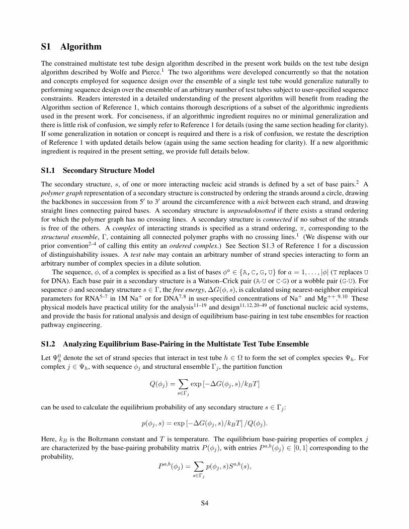
The secondary structure, s, of one or more interacting nucleic acid strands is defined by a set of base pairs.2 Apolymer graph representation of a secondary structure is constructed by ordering the strands around a circle, drawingthe backbones in succession from 50 to 30 around the circumference with a nick between each strand, and drawingstraight lines connecting paired bases. A secondary structure is unpseudoknotted if there exists a strand orderingfor which the polymer graph has no crossing lines. A secondary structure is connected if no subset of the strandsis free of the others. A complex of interacting strands is specified as a strand ordering, ⇡, corresponding to thestructural ensemble, Γ, containing all connected polymer graphs with no crossing lines.1 (We dispense with ourprior convention2–4 of calling this entity an ordered complex.) See Section S1.3 of Reference 1 for a discussionof distinguishability issues. A test tube may contain an arbitrary number of strand species interacting to form anarbitrary number of complex species in a dilute solution.
The sequence, φ, of a complex is specified as a list of bases φa 2 {A,C,G,U} for a = 1, . . . , |φ| (T replaces Ufor DNA). Each base pair in a secondary structure is a Watson–Crick pair (A·U or C·G) or a wobble pair (G·U). Forsequence φ and secondary structure s 2 Γ, the free energy, ∆G(φ, s), is calculated using nearest-neighbor empiricalparameters for RNA5–7 in 1M Na+ or for DNA7, 8 in user-specified concentrations of Na+ and Mg++.9, 10 Thesephysical models have practical utility for the analysis11–19 and design11, 12, 20–49 of functional nucleic acid systems,and provide the basis for rational analysis and design of equilibrium base-pairing in test tube ensembles for reactionpathway engineering.
S1.2 Analyzing Equilibrium Base-Pairing in the Multistate Test Tube Ensemble
Let 0
h
denote the set of strand species that interact in test tube h 2 ⌦ to form the set of complex species h
. Forcomplex j 2
h
, with sequence φj
and structural ensemble Γ
j
, the partition function
Q(φj
) =
X
s2Γj
exp [−∆G(φj
, s)/kB
T ]
can be used to calculate the equilibrium probability of any secondary structure s 2 Γ
j
:
p(φj
, s) = exp [−∆G(φj
, s)/kB
T ] /Q(φj
).
Here, kB
is the Boltzmann constant and T is temperature. The equilibrium base-pairing properties of complex jare characterized by the base-pairing probability matrix P (φ
j
), with entries P a,b
(φj
) 2 [0, 1] corresponding to theprobability,
P a,b
(φj
) =
X
s2Γj
p(φj
, s)Sa,b
(s),
S4
that base pair a ·b forms at equilibrium within ensemble Γj
. Here, S(s) is a structure matrix with entries Sa,b
(s) = 1
if structure s contains base pair a · b and Sa,b
(s) = 0 otherwise. For convenience, the structure and probabilitymatrices are augmented with an extra column to describe unpaired bases. The entry Sa,|s|+1
(s) is unity if base a isunpaired in structure s and zero otherwise; the entry P a,|j |+1
(φj
) 2 [0, 1] denotes the equilibrium probability thatbase a is unpaired over ensemble Γ
j
. Hence the row sums of the augmented S(s) and P (φj
) matrices are unity.Let Q
h⌘ Q
j
8j 2
h
denote the set of partition functions for the complexes in tube h. The set of equilib-rium concentrations, x
h, h, (specified as mole fractions) are the unique solution to the strictly convex optimization
problem:2
min
xh, h
X
j2 h
xh,j
(log xh,j
− logQj
− 1) (S1a)
subject to Ai,j
xh,j
= x0h,i
8i 2
0
h
, (S1b)
where the constraints impose conservation of mass. A is the stoichiometry matrix with entries Ai,j
corresponding tothe number of strands of type i in complex j, and x0
h,i
is the total concentration of strand i introduced to test tube h.To analyze the equilibrium base-pairing properties of all test tubes h 2 ⌦, the partition function, Q
j
, andequilibrium pair probability matrix, P
j
, must be calculated for each complex j 2 using ⇥(|φj
|3) dynamic pro-grams.2, 50–57 The equilibrium concentrations, x
h, h8h 2 ⌦, are calculated by solving a convex programming
problem using an efficient trust region method at a cost that is typically negligible by comparison.2 The overall timecomplexity to analyze the test tubes in ⌦ is then O(| ||φ|3
max
), where |φ|max
is the size of the largest complex.Evaluation of the multistate test tube ensemble defect, M, requires calculation of the complex partition func-
tions, Q
, which are used to calculate the equilibrium concentrations, xh, h
8h 2 ⌦, as well as the equilibrium pairprobability matrices, P
on , which are used to calculate the complex ensemble defects, n
on , and the normalized testtube ensemble defects, M
⌦
. Hence, the time complexity to evaluate the design objective function over the set oftarget test tubes, ⌦, is the same as the time complexity to analyze equilibrium base-pairing in ⌦.
S1.3 Test Tube Ensemble Focusing
To reduce the cost of sequence optimization, the set of complexes, , is partitioned into two disjoint sets:
=
active [
passive,
where
active denotes complexes that will be actively designed and
passive denotes complexes that will inheritsequence information from
active. Only the complexes in
active are directly accounted for in the focused test tubeensembles that are used to evaluate candidate sequences. Initially, we set
active
=
on,
passive
=
o↵ , (S2)
where
on ⌘ [h2⌦
on
h
is the set of complexes that appear as on-targets in at least one test tube, and
o↵ ⌘ −
on
is the set of complexes that appear as off-targets in at least one test tube and do not appear as on-targets in any testtube. Hence, with test tube ensemble focusing, only complexes that are on-targets in at least one test tube are activelydesigned at the outset of sequence design.
S5
S1.4 Hierarchical Ensemble Decomposition
To enable efficient estimation of test tube ensemble properties, the structural ensemble Γ
j
of each complex j 2
active is hierarchically decomposed into a (possibly unbalanced) binary tree of conditional subensembles, yieldinga forest of decomposition trees. Each complex j 2
active contributes a single tree to the decomposition forestwhether it is contained in one or more tubes h 2 ⌦. The structural ensemble of each parent node within the forest isdecomposed using one or more exclusive split-points to partition the parent nucleotides to its children. See Reference1 for details on hierarchical ensemble decomposition. Let ⇤ denote the set of all nodes in the forest. Let ⇤
d
denotethe set of all nodes at depth d.
S1.4.1 Structure-Guided Decomposition of On-Target Complexes
At the outset of sequence design, equilibrium base-pairing probabilities are not yet available to guide ensembledecomposition. Instead, structure-guided hierarchical ensemble decomposition is performed (using a single split-point per parent) for each on-target complex j 2
active, yielding a forest of | on| decomposition trees. SeeReference 1 for details on structure-guided decomposition.
S1.4.2 Stop Condition Stringency
In order to build in a tolerance for a basal level of decomposition defect as subsequences are merged moving up thedecomposition forest, the stringency of the stop condition (3) is increased by a factor of f
stringent
2 (0, 1) at eachlevel moving down the decomposition forest:
f stop
d
⌘ fstop
(fstringent
)
d−1 8d 2 {1, . . . , D}.
S1.5 Efficient Estimation of Test Tube Ensemble Properties
During sequence optimization, the design objective function is estimated based on physical quantities calculatedefficiently at any depth d 2 {1, . . . , D} in the decomposition forest.
S1.5.1 Complex Partition Function Estimate
For each complex j 2
active, the complex partition function estimate, ˜Qj
, is calculated from conditional partitionfunctions evaluated efficiently at any depth d 2 {1, . . . , D} as described in Reference 1.
S1.5.2 Complex Pair Probability Matrix Estimate
For each complex j 2
active, the complex pair probability matrix estimate, ˜Pj
, is calculated from conditional pairprobability matrices evaluated efficiently at any depth d 2 {1, . . . , D} as described in Reference 1.
S1.5.3 Complex Concentration Estimate using Deflated Mass Constraints
For each tube h 2 ⌦, the complex concentration estimates, xh,
active
h, are calculated using the complex partition
function estimates ˜Q
active
hpreviously evaluated at any depth d 2 {1, . . . , D} as described in Reference 1. Deflated
mass constraints are used to model the effect of the neglected off-target complexes in
passive
h
.
S1.5.4 Complex Ensemble Defect Estimate
For each complex j 2
on, the complex ensemble defect estimate, nj
, is calculated using the complex pair probabil-ity matrix estimate ˜P
j
previously evaluated at any depth d 2 {1, . . . , D} as described in Reference 1. For complex
S6
j, the contribution of nucleotide a to the complex ensemble defect estimate is given by:
na
j
= 1−X
1b|j |+1
˜P a,b
j
Sa,b
j
and the complex ensemble defect estimate is then:
nj
=
X
1a|j |
na
j
. (S3)
S1.5.5 Test Tube Ensemble Defect Estimate
For each tube h 2 ⌦, the test tube ensemble defect estimate based on xh,
active
hand n
on
hcalculated at any depth
d 2 {1, . . . , D}, is:˜Ch
=
X
j2 on
h
ch,j
, (S4)
where
ch,j
= nj
min (xh,j
, yh,j
) + |φj
|max (yh,j
− xh,j
, 0) (S5)
is the contribution of complex j. The normalized test tube ensemble defect estimate for tube h 2 ⌦ at depthd 2 {1, . . . , D} is then:
˜Mh
=
˜Ch
/ynth
, (S6)
whereynth
=
X
j2 on
h
|φj
|yh,j
is the total concentration of nucleotides in tube h.
S1.5.6 Multistate Test Tube Ensemble Defect Estimate
For the set of target test tubes ⌦, the objective function estimate based on ˜M⌦
evaluated at any depth d 2 {1, . . . , D}is then:
˜M =
1
|⌦|X
h2⌦
˜Mh
. (S7)
We write ˜Md
in subsequent equations where it is helpful note the depth d at which ˜M was calculated.Note that equations (S3)–(S7) may be collected into the single equation:
˜M =
X
h2⌦
X
j2 on
h
X
1a|j |
˜Ma
h,j
(S8)
where˜Ma
h,j
⌘ 1
|⌦|ynth
⇥na
j
min(xh,j
, yh,j
) + max(yh,j
− xh,j
, 0)⇤, (S9)
is the contribution of nucleotide a in complex j 2
on
h
in tube h 2 ⌦ to the multistate test tube ensemble defectestimate, ˜M, evaluated at any depth d 2 {1, . . . , D}. This representation is convenient when defining objectivefunction weights (Section S1.6) and when defining defect-weighted mutation sampling during leaf mutation anddefect-weighted reseeding during leaf reoptimization (Sections S1.7.2 and S1.7.3).
S7
S1.6 Adjusting Design Priorities using Defect Weights
The user may adjust design priorities by specifying weights for contributions to the multistate test tube ensembledefect estimate, ˜M:
• Nucleotide weight: wa
h,j
weights the contribution of nucleotide a in complex j 2
on
h
in tube h 2 ⌦.• Complex weight: w
h,j
weights the contribution of complex j 2
on
h
in tube h 2 ⌦ (equivalent to setting wa
h,j
for all nucleotides 1 a |φj
|).• Test tube weight: w
h
weights the contribution of tube h 2 ⌦ (equivalent to setting wh,j
for all complexesj 2
on
h
).
Each weight takes a value in the interval [0,1). By default, all weights are unity. Increasing the weight for anucleotide, complex, or test tube will lead to a corresponding increase in the allocation of effort to designing thisentity, typically leading to a corresponding reduction in the defect contribution of the entity. Likewise, decreasingthe weight for a nucleotide, complex, or test tube will lead to a corresponding decrease in the allocation of effort todesigning this entity, typically leading to a corresponding increase in the defect contribution of the entity.
Weights are incorporated into the objective function by replacing the defect contribution (S9) with the weighteddefect contribution
˜Ma
h,j
⌘wh
wh,j
wa
h,j
|⌦|ynth
⇥na
j
min(xh,j
, yh,j
) + max(yh,j
− xh,j
, 0)⇤, (S10)
and summing using (S8) as before. If desired, the user can set weights at all three levels, leading to a multiplicativeeffect. The complex weights and test tube weights exist purely for convenience, as their effects can always bereplicated by appropriately setting nucleotide weights (more tediously).
S1.7 Sequence Optimization at the Leaves of the Decomposition Forest
S1.7.1 Initialization
At the outset of sequence optimization, sequences are randomly initialized subject to the constraints in R by solvinga constraint satisfaction problem using a branch and propagate algorithm (Section S1.11.3).
S1.7.2 Leaf Mutation
To minimize computational cost, all candidate mutation sets are evaluated at the leaf nodes, k 2 ⇤
D
, of the decom-position forest. Leaf mutation terminates if the leaf stop condition,
˜MD
f stop
D
, (S11)
is satisfied. Here, ˜MD
denotes the objective function estimated at level D. A candidate mutation set is accepted ifit decreases the objective function estimate (S8) and rejected otherwise.
We perform defect weighted mutation sampling by selecting nucleotide a in complex j 2
on
h
in tube h 2 ⌦ formutation with probability,
˜Ma
h,j
/ ˜MD
, (S12)
proportional to its contribution to the objective function. After selecting a candidate mutation position, a candidatemutation is randomly selected from the set of permitted nucleotides at that position. If the resulting sequence isinfeasible (due to constraint violations caused by the candidate mutation), a feasible candidate sequence, ˆφ
⇤D, is
generated by solving a constraint satisfaction problem using a branch and propagate algorithm (Section S1.11.4).A feasible candidate sequence, ˆφ
⇤D, is evaluated via calculation of the objective function estimate, ˜M
D
, if thecandidate mutation set, ⇠, is not in the set of previously rejected mutation sets, γ
bad
. The set, γbad
, is updated aftereach unsuccessful mutation and cleared after each successful mutation. The counter m
bad
is used to keep track ofthe number of consecutive failed mutation attempts; it is incremented after each unsuccessful mutation and reset tozero after each successful mutation. Leaf mutation terminates unsuccessfully if m
bad
≥ Mbad
. The outcome of leafmutation is the feasible sequence, φ
⇤D, corresponding to the lowest encountered ˜M
D
.
S8
S1.7.3 Leaf Reoptimization
After leaf mutation terminates, if the leaf stop condition (S11) is not satisfied, leaf reoptimization commences. At theoutset of each round of leaf reoptimization, we perform defect-weighted reseeding of M
reseed
positions by selectingnucleotide a for reseeding (with a new random initial sequence) with probability (S12). Following reseeding, afeasible candidate sequence, ˆφ
⇤D, is generated by solving a constraint satisfaction problem using a branch and
propagate algorithm (Section S1.11.5). After a new round of leaf mutation starting from this reseeded feasiblesequence, the reoptimized candidate sequence, ˆφ
⇤D, is accepted if it decreases ˜M
D
and rejected otherwise. Thecounter m
reopt
is used to keep track of the number of rounds of leaf reoptimization; mreopt
is incremented aftereach rejection and reset to zero after each acceptance. Leaf reoptimization terminates successfully if the leaf stopcondition is satisfied and unsuccessfully if m
reopt
≥ Mreopt
. The outcome of leaf reoptimization is the feasiblesequence, φ
⇤D, corresponding to the lowest encountered ˜M
D
.
S1.8 Subsequence Merging, Redecomposition, and Reoptimization
Moving down the decomposition forest, hierarchical ensemble decomposition makes the assumption that base pairssandwiching parental split-points form with probability approaching unity. Conditional child ensembles enforcethese sandwiching base pairs at all levels in the decomposition forest in accordance with the decomposition assump-tion. As subsequences are merged moving up the decomposition forest, the accuracy of the decomposition assump-tion is checked. If the assumption is correct, the child-estimated defect will accurately predict the parent-estimateddefect. If the assumption is incorrect, the child-estimated defect will not accurately predict the parent-estimateddefect since the conditional child ensembles neglect the contributions of structures that lack the sandwiching basepairs. During subsequence merging, if the decomposition assumption is discovered to be incorrect, hierarchical en-semble redecomposition is performed based on the newly available parental base-pairing information. The detailsof subsequence merging, redecomposition, and reoptimization are as follows.
After leaf reoptimization terminates, parent nodes at depth d = D− 1 merge their left and right child sequencesto create the candidate sequence ˆφ
⇤d. The parental objective function estimate, ˜M
d
, is calculated and the candidatesequence, ˆφ
⇤d, is accepted if it decreases ˜M
d
and rejected otherwise. If the parental stop condition
˜Md
max(f stop
d
, ˜Md+1
/fstringent
) (S13)
is satisfied, merging continues up to the next level in the forest. Otherwise, failure to satisfy the parental stopcondition indicates the existence of the decomposition defect,
˜Md
− ˜Md+1
/fstringent
> 0,
exceeding the basal level permitted by the parameter fstringent
. The parent node at depth d whose replacement byits children results in the greatest underestimate of the objective function at level d is subjected to structure- andprobability-guided hierarchical ensemble decomposition (Section S1.10.2). Additional parents are redecomposeduntil
˜Md
− ˜M⇤d+1
/fstringent
fredecomp
(
˜Md
− ˜Md+1
/fstringent
)
where ˜Md+1
is the child defect estimate before any redecomposition, ˜M⇤d+1
is the child defect estimate afterredecomposition, and f
redecomp
2 (0, 1).After redecomposition, the current sequences at depth d are pushed to level D, the lowest encountered defect
estimate is reset for all levels below d, and a new round of leaf mutation and leaf reoptimization is performed. Fol-lowing leaf reoptimization, merging begins again. Subsequence merging and reoptimization terminate successfullyif the parental stop condition (S13) is satisfied at depth d = 1. The outcome of subsequence merging, redecomposi-tion, and reoptimization is the feasible sequence, φ
⇤
1
, corresponding to the lowest encountered ˜M1
.
S9
S1.9 Test Tube Evaluation, Refocusing, and Reoptimization
Using test tube ensemble focusing, initial sequence optimization is performed for the on-target complexes in
active,neglecting the off-target complexes in
passive. At the termination of initial forest optimization, the estimated designobjective function is ˜M
1
, calculated using (S8). The estimated contributions for each tube h 2 ⌦ are based oncomplex concentration estimates, x
h,
active
h, calculated using deflated total strand concentrations (equation (10) of
Reference 1) to create a built-in defect allowance for the effect of the neglected off-targets in
passive
h
. The exactdesign objective function, M, is then evaluated for the first time over the full ensemble . For this exact calculation,the objective function, M, is based on complex concentrations, x
h, h, calculated using the full strand concentrations
(equation (9) of Reference 1).If the objective function satisfies the termination stop condition,
M max(fstop
, ˜M1
), (S14)
sequence design terminates successfully. Otherwise, failure to satisfy the termination stop condition indicates theexistence of the focusing defect,
M− ˜M1
> 0. (S15)
The multistate test tube ensemble is refocused by transferring the highest-concentration off-target in
passive to
active. Additional off-targets are transferred from
passive to
active until
M− ˜M⇤1
frefocus
(M− ˜M1
), (S16)
where ˜M1
is the forest-estimated defect before any refocusing, ˜M⇤1
is the forest-estimated defect after refocusing(calculated using deflated total strand concentrations (equation (10) of Reference 1) if passive 6= ;), and f
refocus
2(0, 1).
The new off-targets in
active are then decomposed using probability-guided hierarchical ensemble decomposi-tion (Section S1.10.1), the decomposition forest is augmented with new nodes at all depths, and forest reoptimizationcommences starting from the final sequences from the previous round of forest optimization. During forest reopti-mization, the algorithm actively attempts to destabilize the off-targets that were added to
active. This process of testtube ensemble refocusing and forest reoptimization is repeated until the termination stop condition (S14) is satisfied,which is guaranteed to occur in the event that all off-targets are eventually added to
active. At the conclusion ofsequence design, the algorithm returns the feasible sequence set, φ
, that yielded the lowest encountered objectivefunction, M.
S1.10 Hierarchical Ensemble Decomposition Using Multiple Exclusive Split-Points
Prior to sequence optimization, in the absence of base-pairing probability information, hierarchical ensemble decom-position is performed for each complex j 2
active based on user-specified target structures. During subsequencemerging, if decomposition defects are encountered, or during test tube evaluation, if focusing defects are encoun-tered, subsequent hierarchical ensemble decomposition takes advantage of the newly available parental base-pairingprobabilities. In either case, selection of the optimal set of exclusive split-points is determined using a branch andbound algorithm to minimize the cost of evaluating the child nodes (see Section S1.4 of Reference 1).
S1.10.1 Probability-Guided Decomposition using Multiple Exclusive Split-Points
During redecomposition (Section S1.8) and refocusing (Section S1.9), parent nodes that lack a target structure aredecomposed via probability-guided decomposition using multiple exclusive split-points. See Reference 1 for detailson probability-guided decomposition.
S1.10.2 Structure- and Probability-Guided Decomposition using Multiple Exclusive Split-Points
During redecomposition (Section S1.8), parent nodes that have a target structure are decomposed via structure- andprobability-guided decomposition using multiple exclusive split-points. See Reference 1 for details on structure-and probability-guided decomposition.
S10

Table S1. IUPAC degenerate nucleotide codes for RNA.
Code Nucleotides
M A or CR A or GW A or US C or GY C or UK G or UV A, C, or GH A, C, or UD A, G, or UB C, G, or UN A, C, G, or U
T replaces U for DNA.
S1.10.3 Multistate Test Tube Ensemble Defect Estimate Using Multiple Exclusive Decompositions
Because exclusive split-points lead to exclusive structural ensembles, the expressions used to estimate ensembleproperties over ⌦ (Section S1.5) can be generalized to account for the possibility of multiple exclusive split-pointswithin any parent in the decomposition forest. See Reference 1 for details.
S1.11 Generation of Feasible Sequences
Each time the sequence is initialized, mutated, or reseeded, a feasible sequence is generated by solving a constraintsatisfaction problem based on the user-specified constraints in R.
S1.11.1 Constraint Satisfaction Problem
A constraint satisfaction problem (CSP)58 is specified as:
• a set of variables,• a set of domains, each listing the possible values for the corresponding variable,• a set of constraints, each defined by a constraint relation operating on a subset of the variables.
In the present setting, each variable is the sequence, φa, of a nucleotide, a. For RNA, the domain for each variable is{A,C,G,U}. Each constraint in R is specified using one of the constraint relations in Table 1 applied to one or morenucleotides (e.g., specification of constraint Rmatch
a,b
requires that φa
= φb for nucleotides a and b).In general, constraint satisfaction problems are NP-complete, so general-purpose polynomial-time algorithms
are unavailable.58 Empirically, we find that CSPs arising in the context of nucleic acid reaction pathway engineeringspecified in terms of the diverse constraint relations of Table 1 can typically be solved efficiently using the branchand propagate algorithm described below.
S1.11.2 Branch and Propagate Algorithm
We solve the CSP using a branch and propagate algorithm that returns a solution if one exists and returns a warningif no solution exists. Initially, the domain for each variable is {A,C,G,U}. We first pre-process the CSP by triviallyremoving any value from the domain of a variable a that is inconsistent with a constraint (e.g., an assignmentor library constraint). We further pre-process the CSP using constraint propagation to impose arc consistency asdescribed below.
The branch and propagate algorithm involves iterated application of two ingredients:
S11
• constraint propagation is used to narrow the search space by imposing arc consistency on each pair of vari-ables: for any value in the domain of variable a there must be a consistent value in the domain of every othervariable b, otherwise that value of variable a is inconsistent and can be removed from the domain of a (see“Chapter 3: Consistency-Enforcing and Constraint Propagation” of Reference 58).
• depth-first branching is used to extend a candidate partial solution by assigning a consistent value to oneadditional variable a, followed by backtracking to reassign the value of the most-recently assigned variable ifno value in the domain of a is consistent with previous assignments (see “Chapter 5: General Search Strategies:Look-Ahead” of Reference 58).
S1.11.3 Feasible Sequence Inititialization
Sequence initialization (Section S1.7.1) commences with constraint propagation to impose arc consistency and thena first branching step in which a variable, a, is randomly selected and randomly assigned a value from the domain ofa. Constraint propagation is then used to impose arc consistency and the next branching step is taken by randomlyselecting an unassigned variable, b, and assigning a consistent value from the domain of b. Backtracking is performedif no consistent value for b exists. The branch and propagate algorithm returns a feasible set of initial sequences,φ
active
, if one exists, and a warning otherwise.
S1.11.4 Feasible Sequence Mutation
During leaf mutation (Section S1.7.2), a feasible candidate sequence is generated by mutating the current leaf se-quence, φ
⇤D. This process begins with the sequence design algorithm randomly selecting a nucleotide a for mutation
with probability (S12) and randomly assigning a new value from the domain of a. We then solve a CSP to obtaina valid candidate sequence consistent with the new value of a. Constraint propagation is used to impose arc con-sistency with the new value of a and any variables that require reassignment are added to the candidate mutationset, ⇠
a
. Initially, branching is performed by randomly selecting an unassigned variable b from ⇠a
with probabilityproportional to the size of the domain of b (i.e., using weight
wb
= |domain(b)| (S17)
to calculate the probability of selecting b). For each value φb in the domain of b, we check the implications ofarc consistency on the size of the candidate mutation set, ⇠
a,b
, and create a priority queue based on the minimumincrease in |⇠
a,b
| relative to |⇠a
|. Let |⇠a,b
1
| denote the minimum increase, |⇠a,b
2
| denote the next largest increase, andso on. Branching is performed by exploring the values of b according to their rank order in this priority queue. If noconsistent value of b exists, backtracking is performed and the selection weight for variable b (S17) is updated using
wb
= ✏wb
+ (1− ✏)(|⇠a,b
1
|− |⇠a
|). (S18)
where ✏ = 0.5 is a decay constant. The heuristics (S17) and (S18) seek to preferentially select highly constrainedvariables early in the branching process to avoid excessive backtracking. The initial weights (S17) assume that eachvariable b will imply a mutation set ⇠
a,b
that increases in size with the size of domain(b), preferentially selectingvariables with larger domains. With (S18), as we explore different variables b in ⇠
a
, we explicitly calculate theimplied increase in ⇠
a,b
due to each branching decision, and update the weights to bias future searching towardselection of b variables that cause the highest minimal increase in the size of the mutation set ⇠
a
.The branch and propagate algorithm returns a feasible candidate sequence, ˆφ
⇤D, if one exists. Otherwise, the
new value of a is invalid and is removed from the domain of a; a new value of a is randomly selected from thedomain of a, and branch and propagate is applied again. If the only valid value of a is the current value, then m
bad
is incremented and the leaf mutation procedure selects a new nucleotide for mutation with probability (S12).
S1.11.5 Feasible Sequence Reseeding
During leaf reoptimization (Section S1.7.3), a feasible candidate reseeded sequence, ˆφ⇤D
, is generated by intro-ducing M
reseed
feasible sequence mutations to the current leaf sequence, φ⇤D
, via Mreseed
consecutive calls to the
S12

branch and propagate algorithm of Section S1.11.4 (selecting nucleotide a for mutation without replacement withprobability (S12)).
S13
S1.12 Pseudocode
OPTIMIZETUBES(⌦, on
⌦
,
o↵
⌦
, , s
, y
⌦, ,R)
active
,
passive
on
,
o↵
φ
active
INITSEQ(s
active
,R)
⇤, D MAKEFOREST(s
active
)
φ
⇤
,
˜M1
OPTIMIZEFOREST(φ⇤
, D)
M EVALUATEDEFECT(φ
)
ˆ
φ
,
ˆM φ
,Mwhile ˆM > max(f
stop
,
˜M1
)
active
,
passive REFOCUSTUBES( active
,
passive
,
{xh,
passive
h})
⇤, D AUGMENTFOREST(⇤, D,
ˆ
P
active
)
ˆ
φ
⇤
,
˜M1
OPTIMIZEFOREST(ˆφ⇤
, D)
ˆM EVALUATEDEFECT(ˆφ
)
if ˆM < Mφ
,M ˆ
φ
,
ˆMreturn φ
OPTIMIZEFOREST(φ⇤
, D)
˜Md 1 8d 2 {1, . . . , D}β
merge
falsewhile ¬β
merge
φ
⇤D ,
˜MD OPTIMIZELEAVES(φ⇤D , D)
d D − 1
β
merge
truewhile d ≥ 1 and β
merge
ˆ
φ
⇤d MERGESEQ(φ⇤d+1
)
ˆMd ESTIMATEDEFECT(ˆφ⇤d)
if ˆMd <
˜Md
φ
⇤d ,˜Md ˆ
φ
⇤d ,ˆMd
if ˆMd > max(f
stop
d ,
˜Md+1
/f
stringent
)
β
merge
false⇤, D REDECOMPOSEFOREST(⇤, D, s
⇤d ,ˆ
P
⇤d)
φ
⇤D SPLITSEQ(ˆφ⇤d)
˜Md0 1 8d0 2 {d+ 1, . . . , D}d d− 1
return φ
⇤
1
,
˜M1
OPTIMIZELEAVES(φ⇤D , D)
φ
⇤D ,
˜MD MUTATELEAVES(φ⇤D , D)
m
reopt
0
while ˜MD > f
stop
D and m
reopt
< M
reopt
ˆ
φ
⇤D RESEEDSEQ(φ⇤D , { ˜Ma
h,j},R)
ˆ
φ
⇤D ,
ˆMD MUTATELEAVES(ˆφ⇤D , D)
if ˆMD <
˜MD
φ
⇤D ,
˜MD ˆ
φ
⇤D ,
ˆMD
m
reopt
0
elsem
reopt
m
reopt
+ 1
return φ
⇤D , ˜MD
MUTATELEAVES(φ⇤D , D)
˜MD ESTIMATEDEFECT(φ⇤D )
γ
bad
;, m
bad
0
while ˜MD > f
stop
D and m
bad
< M
bad
⇠,
ˆ
φ
⇤D SAMPLEMUTATION(φ⇤D , { ˜Ma
h,j},R)
if ⇠ 2 γ
bad
m
bad
m
bad
+ 1
elseˆMD ESTIMATEDEFECT(ˆφ
⇤D )
if ˆMD <
˜MD
φ
⇤D ,
˜MD ˆ
φ
⇤D ,
ˆMD
γ
bad
;, m
bad
0
elseγ
bad
γ
bad
[ ⇠, m
bad
m
bad
+ 1
return φ
⇤D ,
˜MD
ESTIMATEDEFECT(φ⇤d)
˜
Q
⇤d ,˜
P
⇤d CONDITIONALNODALPROPERTIES(φ⇤d)
˜
Q
active
ESTIMATECOMPLEXPFUNCS( ˜Q⇤d)
˜
P
active
ESTIMATECOMPLEXPAIRPROBS( ˜P⇤d)
for h 2 ⌦
x
0
h, 0
h DEFLATEMASSCONSTRAINTS(x0
h, 0
h)
xh, active
h ESTIMATECOMPLEXCONCS( ˜Q
active
h, x
0
h, 0
h)
{ ˜Mah,j} ESTIMATECONTRIBS( ˜P
on
h, s
on
h, xh, on
h, yh, on
h)
˜Md P
h2⌦
Pj2
on
h
P1a|j |
˜Mah,j
return ˜Md
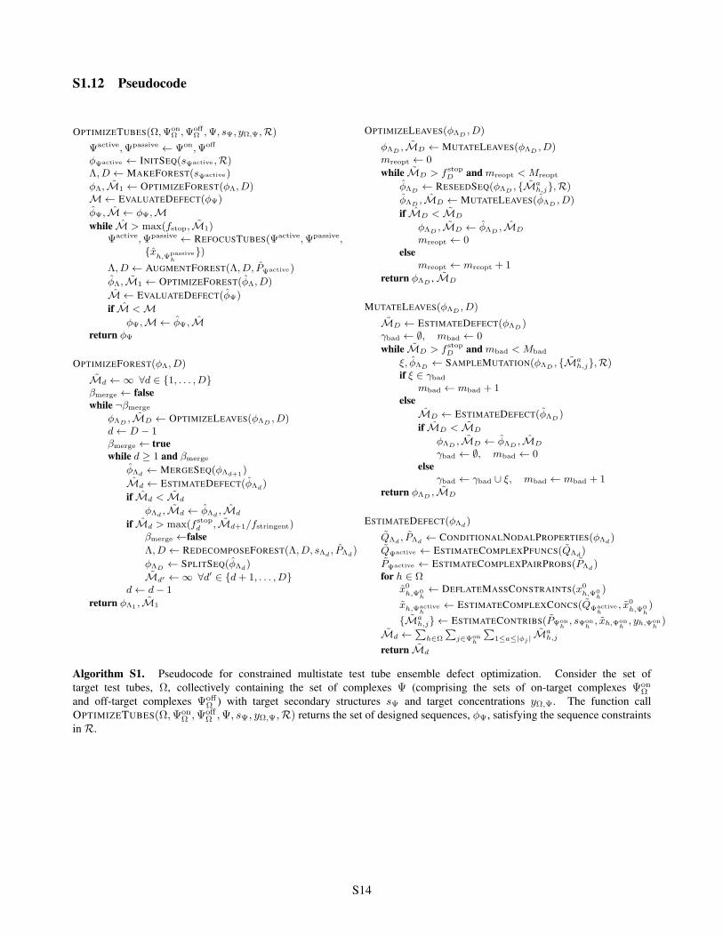
Algorithm S1. Pseudocode for constrained multistate test tube ensemble defect optimization. Consider the set oftarget test tubes, ⌦, collectively containing the set of complexes (comprising the sets of on-target complexes
on
⌦
and off-target complexes
o↵
⌦
) with target secondary structures s
and target concentrations y⌦, . The function call
OPTIMIZETUBES(⌦, on
⌦
, o↵
⌦
, , s
, y⌦, ,R) returns the set of designed sequences, φ
, satisfying the sequence constraintsin R.
S14

S1.13 Default Algorithm Parameters
Default algorithm parameters are shown in Table S2.
Table S2. RNA design: default algorithm parameters for constrained multistate test tube ensemble defect optimization.
Parameter Value
fstop
0.02fpassive
0.01H
split
2
Nsplit
12
fsplit
0.99fstringent
0.99∆Gclamp −25 kcal/molM
bad
300
Mreseed
50
Mreopt
3
fredecomp
0.03frefocus
0.03
For DNA design, Hsplit
= 3.
S15
S2 Engineering Case Studies
S2.1 Reaction Pathways
S2.1.1 Conditional Self-Assembly via Hybridization Chain Reaction (HCR)
A
c*
b*
b
a
A
c*
b*
b
a
b*
a*
X
B
a*
b
b*
c
X·A
c*
b*
b
a
b*
a*
X·A·B
b*
b*
c*
c
b
b
b*
a*
a*
a
X·A·A·B
a*
a
b
b*
c*
c
b*
b
b*
a*a
b
b*
c*
Step 2
Step 1Step 3
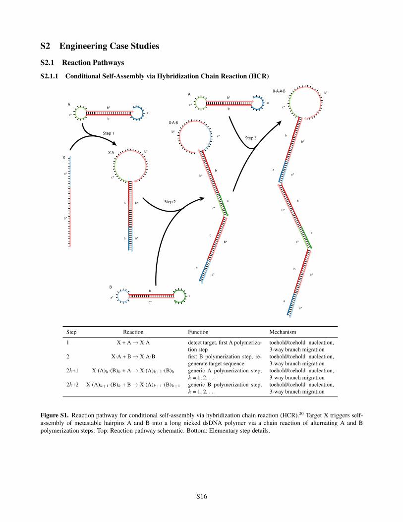
Step Reaction Function Mechanism
1 X + A ! X·A detect target, first A polymeriza-tion step
toehold/toehold nucleation,3-way branch migration
2 X·A + B ! X·A·B first B polymerization step, re-generate target sequence
toehold/toehold nucleation,3-way branch migration
2k+1 X·(A)k·(B)k + A ! X·(A)k+1
·(B)k generic A polymerization step,k = 1, 2, . . .
toehold/toehold nucleation,3-way branch migration
2k+2 X·(A)k+1
·(B)k + B ! X·(A)k+1
·(B)k+1
generic B polymerization step,k = 1, 2, . . .
toehold/toehold nucleation,3-way branch migration
Figure S1. Reaction pathway for conditional self-assembly via hybridization chain reaction (HCR).20 Target X triggers self-assembly of metastable hairpins A and B into a long nicked dsDNA polymer via a chain reaction of alternating A and Bpolymerization steps. Top: Reaction pathway schematic. Bottom: Elementary step details.
S16
S2.1.2 Boolean Logic AND using Toehold Sequestration Gates
Step 1
Step 2Step 3
a* e* f*
e f
h*
gA·B
X·A
B·CY·D
B
X
Y
e f g
a b
a
a* e* f* h*
b
C·D·E
D·E
E
i
d*g*
f*
z y
c*
w
x
w
x
y
z
dc
g* f*
g f
e
d*c*
d
i
c
d*
iz y
c*
w
x
Step Reaction Function Mechanism
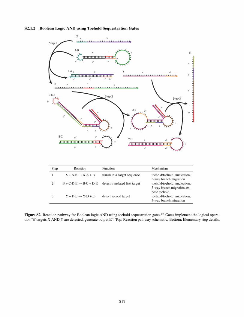
1 X + A·B ! X·A + B translate X target sequence toehold/toehold nucleation,3-way branch migration
2 B + C·D·E ! B·C + D·E detect translated first target toehold/toehold nucleation,3-way branch migration, ex-pose toehold
3 Y + D·E ! Y·D + E detect second target toehold/toehold nucleation,3-way branch migration
Figure S2. Reaction pathway for Boolean logic AND using toehold sequestration gates.59 Gates implement the logical opera-tion “if targets X AND Y are detected, generate output E”. Top: Reaction pathway schematic. Bottom: Elementary step details.
S17
S2.1.3 Self-Assembly of a 3-Arm Junction via Catalytic Hairpin Assembly (CHA)
X
Step 1 Step 2
Step 3b Step 3a
A·B·C
X·A
X·A·B
X·A·B·C
A
B
C
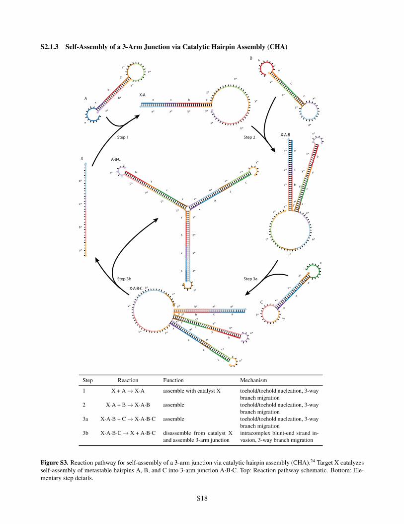
Step Reaction Function Mechanism
1 X + A ! X·A assemble with catalyst X toehold/toehold nucleation, 3-waybranch migration
2 X·A + B ! X·A·B assemble toehold/toehold nucleation, 3-waybranch migration
3a X·A·B + C ! X·A·B·C assemble toehold/toehold nucleation, 3-waybranch migration
3b X·A·B·C ! X + A·B·C disassemble from catalyst Xand assemble 3-arm junction
intracomplex blunt-end strand in-vasion, 3-way branch migration
Figure S3. Reaction pathway for self-assembly of a 3-arm junction via catalytic hairpin assembly (CHA).24 Target X catalyzesself-assembly of metastable hairpins A, B, and C into 3-arm junction A·B·C. Top: Reaction pathway schematic. Bottom: Ele-mentary step details.
S18
S2.1.4 Boolean Logic AND using a Cooperative Hybridization Gate
cbB
ab c
d
a*
b* c*
d*
Y·A·X
a b X
c dY
a
b
b* c*
c d*A·B
Step 1
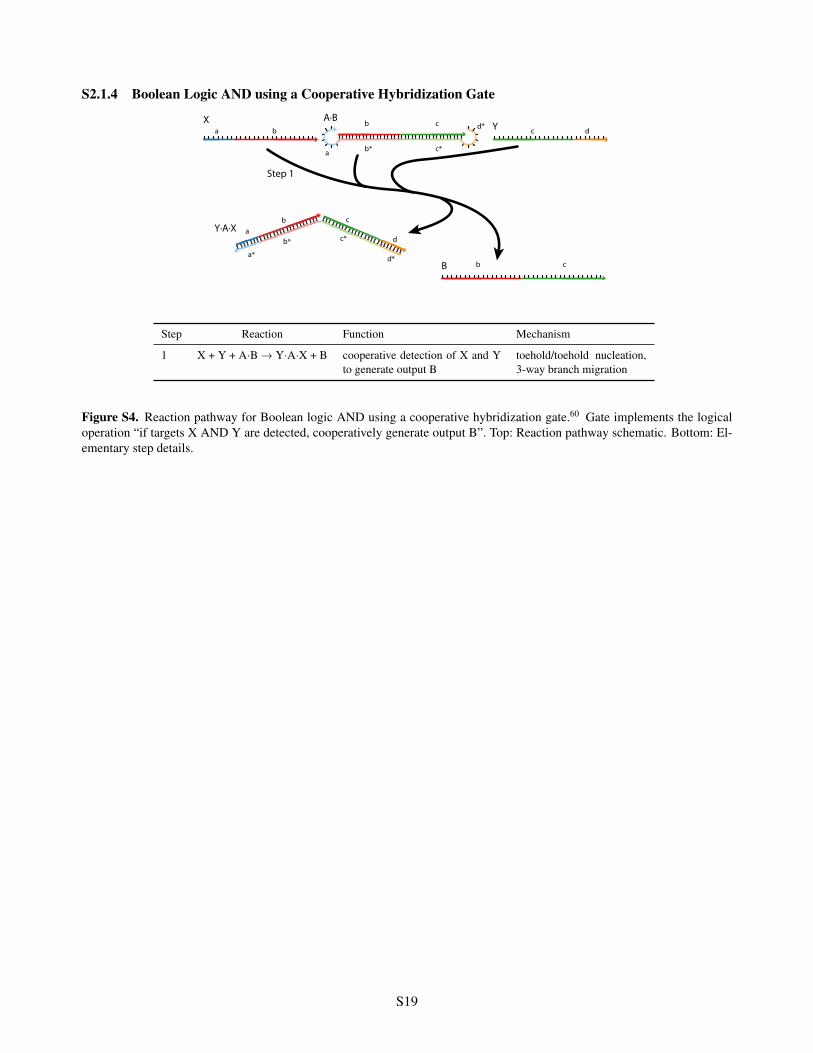
Step Reaction Function Mechanism
1 X + Y + A·B ! Y·A·X + B cooperative detection of X and Yto generate output B
toehold/toehold nucleation,3-way branch migration
Figure S4. Reaction pathway for Boolean logic AND using a cooperative hybridization gate.60 Gate implements the logicaloperation “if targets X AND Y are detected, cooperatively generate output B”. Top: Reaction pathway schematic. Bottom: El-ementary step details.
S19
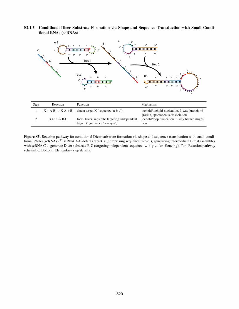
S2.1.5 Conditional Dicer Substrate Formation via Shape and Sequence Transduction with Small Condi-tional RNAs (scRNAs)
Step 1Step 2
C
a b c
a*
y*
z*b* c*
X·A B·C
B
a
b
c
y
x
z
a
b
ys
x w
y*z*
a*x* w*
x y z a
x*w*
y* z* a*
b
w
x
ys
A·By
x
z a b
y* z* a* b*
c*X
Step Reaction Function Mechanism
1 X + A·B ! X·A + B detect target X (sequence ‘a-b-c’) toehold/toehold nucleation, 3-way branch mi-gration, spontaneous dissociation
2 B + C ! B·C form Dicer substrate targeting independenttarget Y (sequence ‘w-x-y-z’)
toehold/loop nucleation, 3-way branch migra-tion
Figure S5. Reaction pathway for conditional Dicer substrate formation via shape and sequence transduction with small condi-tional RNAs (scRNAs).33 scRNA A·B detects target X (comprising sequence ‘a-b-c’), generating intermediate B that assembleswith scRNA C to generate Dicer substrate B·C (targeting independent sequence ‘w-x-y-z’ for silencing). Top: Reaction pathwayschematic. Bottom: Elementary step details.
S20
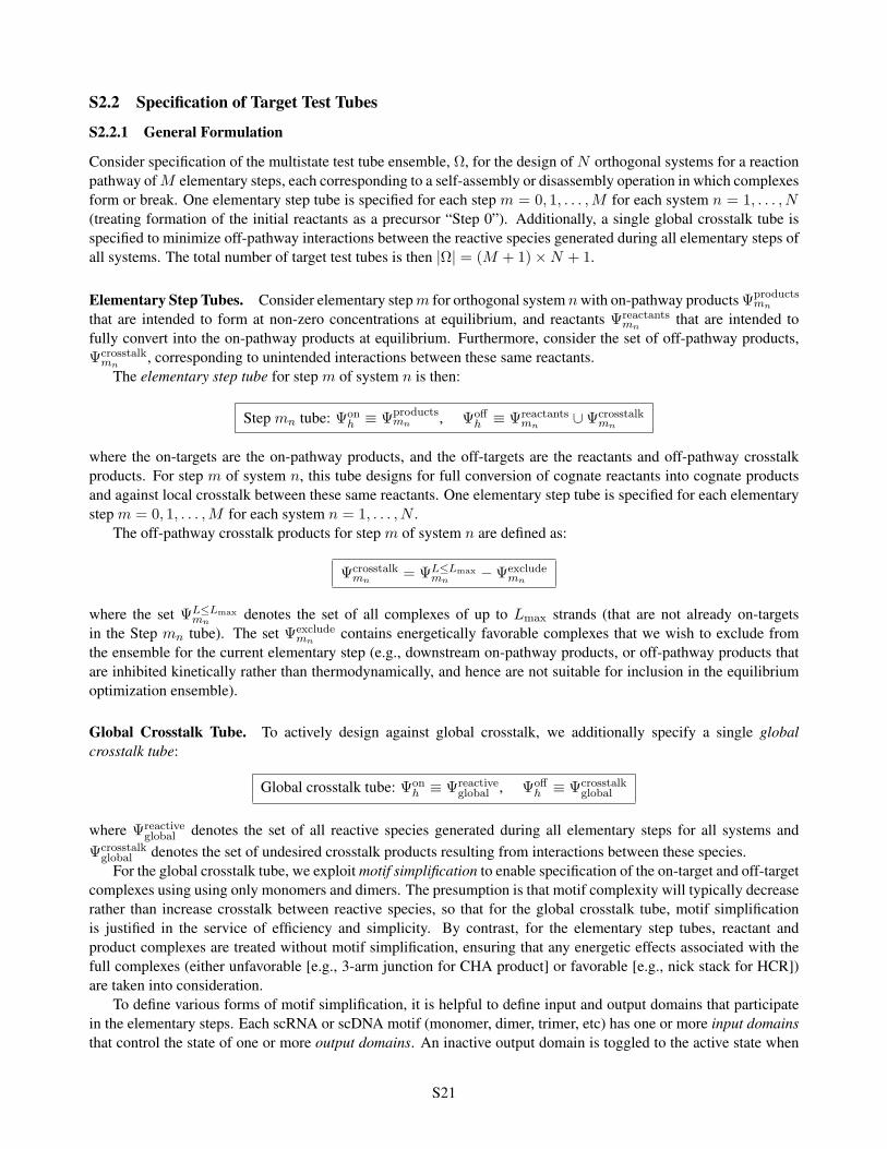
S2.2 Specification of Target Test Tubes
S2.2.1 General Formulation
Consider specification of the multistate test tube ensemble, ⌦, for the design of N orthogonal systems for a reactionpathway of M elementary steps, each corresponding to a self-assembly or disassembly operation in which complexesform or break. One elementary step tube is specified for each step m = 0, 1, . . . ,M for each system n = 1, . . . , N(treating formation of the initial reactants as a precursor “Step 0”). Additionally, a single global crosstalk tube isspecified to minimize off-pathway interactions between the reactive species generated during all elementary steps ofall systems. The total number of target test tubes is then |⌦| = (M + 1)⇥N + 1.
Elementary Step Tubes. Consider elementary step m for orthogonal system n with on-pathway products products
mn
that are intended to form at non-zero concentrations at equilibrium, and reactants
reactants
mnthat are intended to
fully convert into the on-pathway products at equilibrium. Furthermore, consider the set of off-pathway products,
crosstalk
mn, corresponding to unintended interactions between these same reactants.
The elementary step tube for step m of system n is then:
Step mn
tube: on
h
⌘
products
mn ,
o↵
h
⌘
reactants
mn[
crosstalk
mn
where the on-targets are the on-pathway products, and the off-targets are the reactants and off-pathway crosstalkproducts. For step m of system n, this tube designs for full conversion of cognate reactants into cognate productsand against local crosstalk between these same reactants. One elementary step tube is specified for each elementarystep m = 0, 1, . . . ,M for each system n = 1, . . . , N .
The off-pathway crosstalk products for step m of system n are defined as:
crosstalk
mn=
LL
max
mn−
exclude
mn
where the set LL
max
mndenotes the set of all complexes of up to L
max
strands (that are not already on-targetsin the Step m
n
tube). The set exclude
mncontains energetically favorable complexes that we wish to exclude from
the ensemble for the current elementary step (e.g., downstream on-pathway products, or off-pathway products thatare inhibited kinetically rather than thermodynamically, and hence are not suitable for inclusion in the equilibriumoptimization ensemble).
Global Crosstalk Tube. To actively design against global crosstalk, we additionally specify a single globalcrosstalk tube:
Global crosstalk tube: on
h
⌘
reactive
global
,
o↵
h
⌘
crosstalk
global
where
reactive
global
denotes the set of all reactive species generated during all elementary steps for all systems and
crosstalk
global
denotes the set of undesired crosstalk products resulting from interactions between these species.For the global crosstalk tube, we exploit motif simplification to enable specification of the on-target and off-target
complexes using using only monomers and dimers. The presumption is that motif complexity will typically decreaserather than increase crosstalk between reactive species, so that for the global crosstalk tube, motif simplificationis justified in the service of efficiency and simplicity. By contrast, for the elementary step tubes, reactant andproduct complexes are treated without motif simplification, ensuring that any energetic effects associated with thefull complexes (either unfavorable [e.g., 3-arm junction for CHA product] or favorable [e.g., nick stack for HCR])are taken into consideration.
To define various forms of motif simplification, it is helpful to define input and output domains that participatein the elementary steps. Each scRNA or scDNA motif (monomer, dimer, trimer, etc) has one or more input domainsthat control the state of one or more output domains. An inactive output domain is toggled to the active state when
S21
sequestering input domains hybridize to active output domains generated by earlier elementary steps in the reactionpathway. Nucleation with an input domain occurs via hybridization to an accessible loop or toehold. Targets thatserve as inputs to a reaction pathway may be viewed as unconditionally active output domains that are available tohybridize to complementary input domains at any step in a reaction pathway.
Using motif simplification, we specify the reactive species and cognate products for system n as follows:
• λsimple
n
: scRNA and scDNA motifs with multiple input or output domains are simplified so that only the inputand output domains for a single elementary step are present in each simplified motif.
• λss-outn
: single-stranded output domains are specified for each elementary step, removing other concatenatedor hybridized domains that represent the history or future of the reaction (participating in previous or futureelementary steps).
• λss-inn
: single-stranded nucleation sites within input domains (toeholds or loops) are specified isolated from thesurrounding domains representing the history or future of the reaction.⇤
• λreactive
n
⌘ {λsimple [simp
λss-out [simp
λss-in}n
: the set of reactive species for system n is specified using aunion operator [
simp
that eliminates redundancies when one monomer species is an accessible subsequenceof another monomer species.
• λcognate
n
: cognate products expected to form from reactive species in λreactive
n
based on sequence complemen-tarity imposed by the reaction pathway (e.g., an input domain within a motif in λsimple
n
is expected to hybridizeto a complementary output domain in λss-out
n
).
These definitions for λreactive
n
and λcognate
n
are then used to define the on-targets for the global crosstalk tube:
reactive
global
⌘ [n=1,...,N
{λreactive
n
}
and the off-targets for the global crosstalk tube:
crosstalk
global
⌘
LL
max
global
− [n=1,...,N
{λcognate
n
}
Here, LL
max
global
denotes the set of all complexes of up to Lmax
strands (that are not already on-targets in the globalcrosstalk tube). The set [
n=1,...,N
{λcognate
n
} contains all the cognate products that the reactive species in the Northogonal systems are expected to form based on sequence complementarity. Crucially, by excluding these cognateproducts from
crosstalk
global
, they do not appear in the global crosstalk tube as either on-targets or off-targets. Hence,all reactive species in the global crosstalk tube are forced to perform either no reaction (remaining as desired on-targets) or to undergo a crosstalk reaction (forming undesired off-targets), providing the basis for minimization ofglobal crosstalk during sequence optimization.
⇤The role of λss-inn is to enable
crosstalk
global
(the off-targets for the global crosstalk tube) to be specified without requiring any complexeslarger than dimers. For example, consider a dimer motif with an exposed toehold. Crosstalk via kissing of this toehold with that of anotherdimer motif would yield a tetramer off-target; including these toeholds as isolated monomers in λ
ss-inn allows this crosstalk interaction to be
described by an off-target dimer, which is automatically included in
crosstalk
global
by considering all off-targets of up to L
max
= 2 strands.Further, inclusion of loop nucleation sites in λ
ss-inn enables designing against pseudoknotted toehold/loop and loop/loop crosstalk interactions
without needing to explicitly include pseudoknots in the structural ensemble of any complex.
S22

S2.2.2 Conditional Self-Assembly via HCR
Target test tubes are defined using the specification of Section S2.2.1 with the following definitions. The total numberof target test tubes is |⌦| =
Pn=1,...,N
{Step 0, Step 1, Step 2, Step 3}n
+ Crosstalk = 4N + 1; the target test tubesin the multistate test tube ensemble, ⌦, are indexed by h = 1, . . . , 4N + 1. L
max
= 2 for all tubes.
Reactants for system n
• Target: Xn
• Hairpins: {A, B}n
Elementary step tubes for system n
• Step 0n
tube: products
0n⌘ {X, A, B}
n
; reactants
0n⌘ {A·B}
n
(dimer nucleus that inhibits leakage); exclude
0n⌘
{X·A}n
(downstream on-pathway product)
• Step 1n
tube: products
1n⌘ {X·A}
n
; reactants
1n⌘ {X, A}
n
; exclude
1n⌘ ;
• Step 2n
tube: products
2n⌘ {X·A·B}
n
; reactants
2n⌘ {X·A, B}
n
; exclude
2n⌘ ;
• Step 3n
tube: products
3n⌘ {X·A·A·B}
n
; reactants
3n⌘ {X·A·B, A}
n
; exclude
3n⌘ ;
Global crosstalk tube
• Crosstalk tube: reactive
global
⌘ [n=1,...,N
{λreactive
n
};
crosstalk
global
⌘
LL
max
global
− [n=1,...,N
{λcognate
n
}
The reactive species and cognate products for system n are:
• λsimple
n
⌘ {A, B}n
• λss-outn
⌘ {X, Aout, Bout}n
• λss-inn
⌘ {Atoe, Btoe}n
• λreactive
n
⌘ {A, B, Aout, Bout}n
• λcognate
n
⌘ {Aout·B, Bout·A}n
based on the definitions (listed 50 to 30 using the sequence domain notation of Figure S1):
• A ⌘ Ain-Aout
• Atoe ⌘ a• Ain ⌘ a-b• Aout ⌘ c*-b*• B ⌘ Bout-Bin
• Btoe ⌘ c• Bin ⌘ b-c• Bout ⌘ b*-a*• X ⌘ b*-a*
Note: Xn
is identical to Bout
n
, so it is implicitly included in the definition of λreactive
n
. To avoid redundancy, thetoeholds of λss-in
n
are not included in the definition of λreactive
n
; these toeholds are already available to form dimercrosstalk products in the hairpin monomers of λsimple
n
.
S23
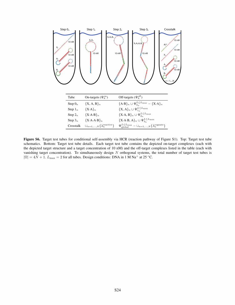
Step 0 Step 1 Step 2 Step 3 Crosstalk
Aout
X ·A ·B
X ·A ·A ·B
10 nM
10 nM
10 nM
10 nM 10 nM 10 nM
A
B
X 10 nM
10 nM
X
X ·A
n = 1,...,N
nn n n n
n
10 nMAn
10 nM
Bn
nnnn
n n n
n n
n
n
n
Tube On-targets ( on
h ) Off-targets ( o↵
h )
Step 0n {X, A, B}n {A·B}n [
LLmax
0n− {X·A}n
Step 1n {X·A}n {X, A}n [
LLmax
1n
Step 2n {X·A·B}n {X·A, B}n [
LLmax
2n
Step 3n {X·A·A·B}n {X·A·B, A}n [
LLmax
3n
Crosstalk [n=1,...,N{λreactive
n }
LLmax
global
− [n=1,...,N{λcognate
n }
Figure S6. Target test tubes for conditional self-assembly via HCR (reaction pathway of Figure S1). Top: Target test tubeschematics. Bottom: Target test tube details. Each target test tube contains the depicted on-target complexes (each withthe depicted target structure and a target concentration of 10 nM) and the off-target complexes listed in the table (each withvanishing target concentration). To simultaneously design N orthogonal systems, the total number of target test tubes is|⌦| = 4N + 1. L
max
= 2 for all tubes. Design conditions: DNA in 1 M Na+ at 25 C.
S24

S2.2.3 Boolean Logic AND using Toehold Sequestration Gates
Target test tubes are defined using the specification of Section S2.2.1 with the following definitions. The total numberof target test tubes is |⌦| =
Pn=1,...,N
{Step 0, Step 1, Step 2, Step 3}n
+ Crosstalk = 4N + 1; the target test tubesin the multistate test tube ensemble, ⌦, are indexed by h = 1, . . . , 4N + 1. L
max
= 2 for all tubes.
Reactants for system n
• Targets: {X, Y}n
• Translator gate: {A·B}n
• AND gate: {C·D·E}n
Elementary step tubes for system n
• Step 0n
: products
0n⌘ {X, Y, A·B, C·D·E}
n
; reactants
0n⌘ {A, B, C, D, E, C·D, D·E}
n
; exclude
0n⌘ {X·A}
n
• Step 1n
: products
1n⌘ {X·A, B}
n
; reactants
1n⌘ {X, A·B}
n
; exclude
1n⌘ ;
• Step 2n
: products
2n⌘ {B·C, D·E}
n
; reactants
2n⌘ {B, C·D·E}
n
; exclude
2n⌘ ;
• Step 3n
: products
3n⌘ {Y·D, E}
n
; reactants
3n⌘ {Y, D·E}
n
; exclude
3n⌘ ;
Global crosstalk tube
• Crosstalk tube: reactive
global
⌘ [n=1,...,N
{λreactive
n
};
crosstalk
global
⌘
LL
max
global
− [n=1,...,N
{λcognate
n
}
The reactive species and cognate products for system n are:
• λsimple
n
⌘ {A·B, C·Dout, D·E}n
• λss-outn
⌘{X, Y, B, Dout, E}n
• λss-inn
⌘ {Atoe, Ctoe, Dtoe}n
• λreactive
n
⌘ {A·B, C·Dout, D·E, X, Y, B, Dout, E, Atoe, Ctoe}n
• λcognate
n
⌘ {X·A, B·C, Y·D, X·Atoe, B·Ctoe}n
based on the definitions (listed 50 to 30 using the sequence domain notation of Figure S2):
• A ⌘ h*-f*-e*-a*• Atoe ⌘ a*• B ⌘ e-f-g• C ⌘ g*-f*• Ctoe ⌘ f*• D ⌘ Dout-Din
• Dtoe ⌘ d*• Din ⌘ c*• Dout ⌘ i-d*• E ⌘ w-x-y-z• X ⌘ a-b• Y ⌘ c-d
Note: Dtoe
n
is contained in Dout
n
, providing a toehold adjacent to Din
n
. To avoid redundancy, we omit Dtoe
n
fromλreactive
n
because it is a subsequence of Dout
n
in λss-outn
.
S25
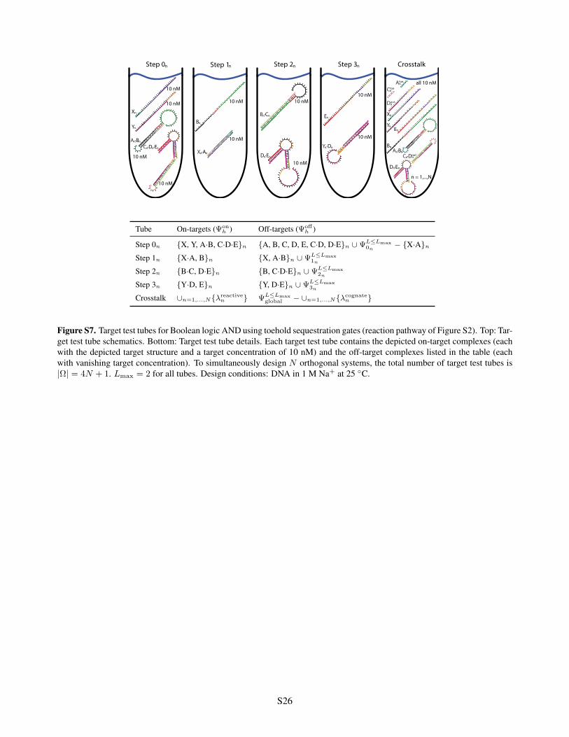
Step 0 Step 3Step 2Step 1 Crosstalk
all 10 nM
10 nM
10 nM
10 nM 10 nM 10 nM
10 nM
10 nM
10 nM
10 nM
10 nM
A ·B
A ·B
X ·AB
BX
Y
X
Y
C ·D ·E
C ·Dout
Atoe
Ctoe
Dout
D ·E
B ·C
D ·E
E
Y ·D
E
n = 1,...,N
n
n
n
n
nn
n
nn
n
nn
n
n
n
n n
n n n
n n
n
n n
nnn
n n
n n n n
Tube On-targets ( on
h ) Off-targets ( o↵
h )
Step 0n {X, Y, A·B, C·D·E}n {A, B, C, D, E, C·D, D·E}n [
LLmax
0n− {X·A}n
Step 1n {X·A, B}n {X, A·B}n [
LLmax
1n
Step 2n {B·C, D·E}n {B, C·D·E}n [
LLmax
2n
Step 3n {Y·D, E}n {Y, D·E}n [
LLmax
3n
Crosstalk [n=1,...,N{λreactive
n }
LLmax
global
− [n=1,...,N{λcognate
n }
Figure S7. Target test tubes for Boolean logic AND using toehold sequestration gates (reaction pathway of Figure S2). Top: Tar-get test tube schematics. Bottom: Target test tube details. Each target test tube contains the depicted on-target complexes (eachwith the depicted target structure and a target concentration of 10 nM) and the off-target complexes listed in the table (eachwith vanishing target concentration). To simultaneously design N orthogonal systems, the total number of target test tubes is|⌦| = 4N + 1. L
max
= 2 for all tubes. Design conditions: DNA in 1 M Na+ at 25 C.
S26

S2.2.4 Self-Assembly of a 3-Arm Junction via CHA
Target test tubes are defined using the specification of Section S2.2.1 with the following definitions. The total numberof target test tubes is |⌦| =
Pn=1,...,N
{Step 0, Step 1, Step 2, Step 3a, Step 3b}n
+ Crosstalk = 5N + 1; the targettest tubes in the multistate test tube ensemble, ⌦, are indexed by h = 1, . . . , 5N + 1. L
max
= 2 for all tubes.
Reactants for system n
• Target: Xn
• Hairpins: {A, B, C}n
Elementary step tubes for system n
• Step 0n
: products
0n⌘ {X, A, B, C}
n
; reactants
0n⌘ ;; exclude
0n⌘ {X·A}
n
• Step 1n
: products
1n⌘ {X·A}
n
; reactants
1n⌘ {X, A}
n
; exclude
1n⌘ ;
• Step 2n
: products
2n⌘ {X·A·B}
n
; reactants
2n⌘ {X·A, B}
n
; exclude
2n⌘ ;
• Step 3an
: products
3an ⌘ {X·A·B·C}n
; reactants
3an ⌘ {X·A·B, C}n
; exclude
3an ⌘ ;• Step 3b
n
: products
3bn ⌘ {X, A·B·C}n
; reactants
3bn ⌘ {X·A·B·C}n
; exclude
3bn ⌘ ;
Note: Step 3 combining an assembly operation (Step 3a; addition of C) with a disassembly operation (Step 3b;removal of X) is described using two target test tubes; the Step 3a tube prevents completion of the full operation byexcluding the final product A·B·C from the ensemble (L
max
= 2 includes all off-targets up to dimers).
Crosstalk tube
• Crosstalk tube: reactive
global
⌘ [n=1,...,N
{λreactive
n
};
crosstalk
global
⌘
LL
max
global
− [n=1,...,N
{λcognate
n
}
The reactive species and cognate products for system n are:
• λsimple
n
⌘ {A, B, C}n
• λss-outn
⌘ {X, Aout, Bout, Cout}n
• λss-inn
⌘ {Atoe, Btoe, Ctoe}n
• λreactive
n
⌘ {A, B, C, X, Aout, Bout, Cout}n
• λcognate
n
⌘ {X·A, Aout·B, Bout·C, Cout·A, Cout·B, Bout·A, Aout·C}n
based on the definitions (listed 50 to 30 using the sequence domain notation of Figure S3):
• A ⌘ Ain-Aout
• Atoe ⌘ a• Ain ⌘ a-x-b-y• Aout ⌘ z*-c*-y*-b*-x*• B ⌘ Bin-Bout
• Btoe ⌘ b• Bin ⌘ b-y-c-z• Bout ⌘ x*-a*-z*-c*-y*• C ⌘ Cin-Cout
• Ctoe ⌘ c• Cin ⌘ c-z-a-x• Cout ⌘ y*-b*-x*-a*-z*• X ⌘ y*-b*-x*-a*
S27
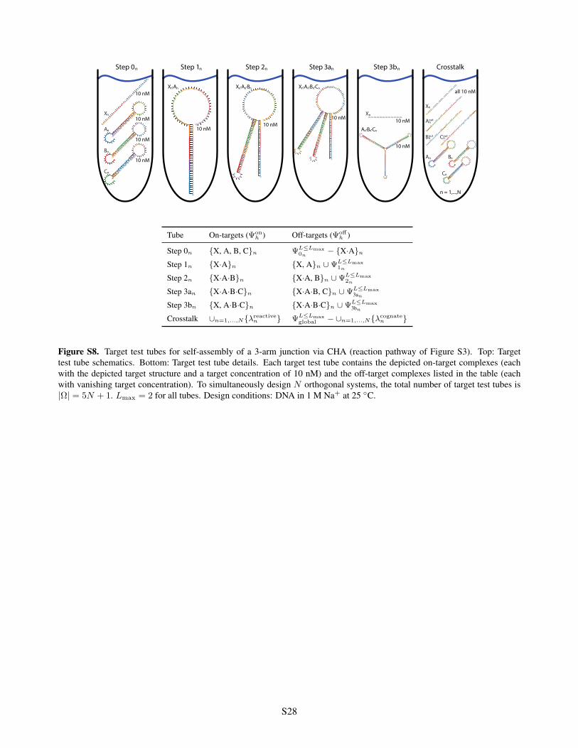
CrosstalkStep 3bStep 0 Step 1 Step 2 Step 3a
10 nM
10 nM
10 nM
10 nM
10 nM 10 nM
10 nM 10 nM
all 10 nM
10 nM
A
Aout
X
Bout Cout
B
C
A
X X
B
C
A ·B ·C
X ·A X ·A ·B X ·A ·B ·C
n = 1,...,N
n
n n n
nn nnnnn
n
n
n
n
n n
n
n n
n
n
n
n
nnnnn
Tube On-targets ( on
h ) Off-targets ( o↵
h )
Step 0n {X, A, B, C}n
LLmax
0n− {X·A}n
Step 1n {X·A}n {X, A}n [
LLmax
1n
Step 2n {X·A·B}n {X·A, B}n [
LLmax
2n
Step 3an {X·A·B·C}n {X·A·B, C}n [
LLmax
3an
Step 3bn {X, A·B·C}n {X·A·B·C}n [
LLmax
3bn
Crosstalk [n=1,...,N{λreactive
n }
LLmax
global
− [n=1,...,N{λcognate
n }
Figure S8. Target test tubes for self-assembly of a 3-arm junction via CHA (reaction pathway of Figure S3). Top: Targettest tube schematics. Bottom: Target test tube details. Each target test tube contains the depicted on-target complexes (eachwith the depicted target structure and a target concentration of 10 nM) and the off-target complexes listed in the table (eachwith vanishing target concentration). To simultaneously design N orthogonal systems, the total number of target test tubes is|⌦| = 5N + 1. L
max
= 2 for all tubes. Design conditions: DNA in 1 M Na+ at 25 C.
S28

S2.2.5 Boolean Logic AND using a Cooperative Hybridization Gate
Target test tubes are defined using the specification of Section S2.2.1 with the following definitions. The total numberof target test tubes is |⌦| =
Pn=1,...,N
{Step 0, Step 1}n
+ Crosstalk = 2N +1; the target test tubes in the multistatetest tube ensemble, ⌦, are indexed by h = 1, . . . , 2N + 1. L
max
= 2 for all tubes.
Reactants for system n
• Targets: {X, Y}n
• Cooperative gate: {A·B}n
Elementary step tubes for system n
• Step 0n
: products
0n⌘ {X, Y, A·B}
n
; reactants
0n⌘ {A·X·B, A·Y·B}
n
; exclude
0n⌘ ;
• Step 1n
: products
1n⌘ {Y·A·X, B}
n
; reactants
1n⌘ {X, Y, A·B}
n
; exclude
1n⌘ ;
Note: Individual targets do not appreciably bind the cooperative gate. In the Step 0n
tube, the reactants are preventedfrom generating the product Y·A·X, because this trimer is excluded from the test tube ensemble (L
max
= 2 includesall off-targets up to dimers).
Crosstalk tube
• Crosstalk tube: reactive
global
⌘ [n=1,...,N
{λreactive
n
};
crosstalk
global
⌘
LL
max
global
− [n=1,...,N
{λcognate
n
}
The reactive species and cognate products for system n are:
• λsimple
n
⌘ {Aleft·Bleft, Aright·Bright}n
• λss-outn
⌘ {X, Y, B}n
• λss-inn
⌘ {Aleft-toe, Aright-toe}n
• λreactive
n
⌘ {Aleft·Bleft, Aright·Bright, X, Y, B, Aleft-toe, Aright-toe}n
• λcognate
n
⌘ {X·Aleft, Y·Aright, X·Aleft-toe, Y·Aright-toe, Aleft·B, Aright·B}n
based on the definitions (listed 50 to 30 using the sequence domain notation of Figure S4):
• A ⌘ Aright-Aleft
• Aleft-toe ⌘ a*• Aleft ⌘ b*-a*• Aright-toe ⌘ d*• Aright ⌘ d*-c*• B ⌘ Bleft-Bright
• Bleft ⌘ b• Bright ⌘ c• X ⌘ a-b• Y ⌘ c-d
S29
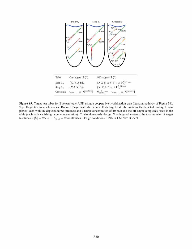
Step 0 Step 1 Crosstalk
10 nM
10 nM
10 nM
10 nM
10 nM
10 nM
10 nM
10 nM 10 nM
10 nM
10 nM
10 nM
A ·B
Y ·A ·X
BB
X X Y
Y
Aleft-toe
Aright-toe
Aleft ·Bleft
Aright ·Bright
n = 1,...,N
n
n
n
n
n
n
n n
n n
n
n
n
n
n
n n
n n
Tube On-targets ( on
h ) Off-targets ( o↵
h )
Step 0n {X, Y, A·B}n {A·X·B, A·Y·B}n [
LLmax
0n
Step 1n {Y·A·X, B}n {X, Y, A·B}n [
LLmax
1n
Crosstalk [n=1,...,N{λreactive
n }
LLmax
global
− [n=1,...,N{λcognate
n }
Figure S9. Target test tubes for Boolean logic AND using a cooperative hybridization gate (reaction pathway of Figure S4).Top: Target test tube schematics. Bottom: Target test tube details. Each target test tube contains the depicted on-target com-plexes (each with the depicted target structure and a target concentration of 10 nM) and the off-target complexes listed in thetable (each with vanishing target concentration). To simultaneously design N orthogonal systems, the total number of targettest tubes is |⌦| = 2N + 1. L
max
= 2 for all tubes. Design conditions: DNA in 1 M Na+ at 25 C.
S30
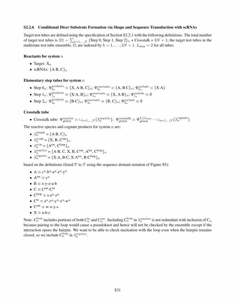
S2.2.6 Conditional Dicer Substrate Formation via Shape and Sequence Transduction with scRNAs
Target test tubes are defined using the specification of Section S2.2.1 with the following definitions. The total numberof target test tubes is |⌦| =
Pn=1,...,N
{Step 0, Step 1, Step 2}n
+ Crosstalk = 3N + 1; the target test tubes in themultistate test tube ensemble, ⌦, are indexed by h = 1, . . . , 3N + 1. L
max
= 2 for all tubes.
Reactants for system n
• Target: Xn
• scRNAs: {A·B, C}n
Elementary step tubes for system n
• Step 0n
: products
0n⌘ {X, A·B, C}
n
; reactants
0n⌘ {A, B·C}
n
; exclude
0n⌘ {X·A}
• Step 1n
: products
1n⌘ {X·A, B}
n
; reactants
1n⌘ {X, A·B}
n
; exclude
1n⌘ ;
• Step 2n
: products
2n⌘ {B·C}
n
; reactants
2n⌘ {B, C}
n
; exclude
2n⌘ ;
Crosstalk tube
• Crosstalk tube: reactive
global
⌘ [n=1,...,N
{λreactive
n
};
crosstalk
global
⌘
LL
max
global
− [n=1,...,N
{λcognate
n
}
The reactive species and cognate products for system n are:
• λsimple
n
= {A·B, C}n
• λss-outn
= {X, B, Cout}n
• λss-inn
= {Atoe, Cloop}n
• λreactive
n
= {A·B, C, X, B, Cout, Atoe, Cloop}n
• λcognate
n
= {X·A, B·C, X·Atoe, B·Cloop}n
based on the definitions (listed 50 to 30 using the sequence domain notation of Figure S5):
• A ⌘ c*-b*-a*-z*-y*• Atoe ⌘ c*• B ⌘ x-y-z-a-b• C ⌘ Cout-Cin
• Cloop ⌘ s-a*-z*• Cin ⌘ a*-z*-y*-x*-w*• Cout ⌘ w-x-y-s• X ⌘ a-b-c
Note: Cloop
n
includes portions of both Cin
n
and Cout
n
. Including Cloop
n
in λreactive
n
is not redundant with inclusion of Cn
because pairing to the loop would cause a pseudoknot and hence will not be checked by the ensemble except if theinteraction opens the hairpin. We want to be able to check nucleation with the loop even when the hairpin remainsclosed, so we include Cloop
n
in λreactive
n
.
S31
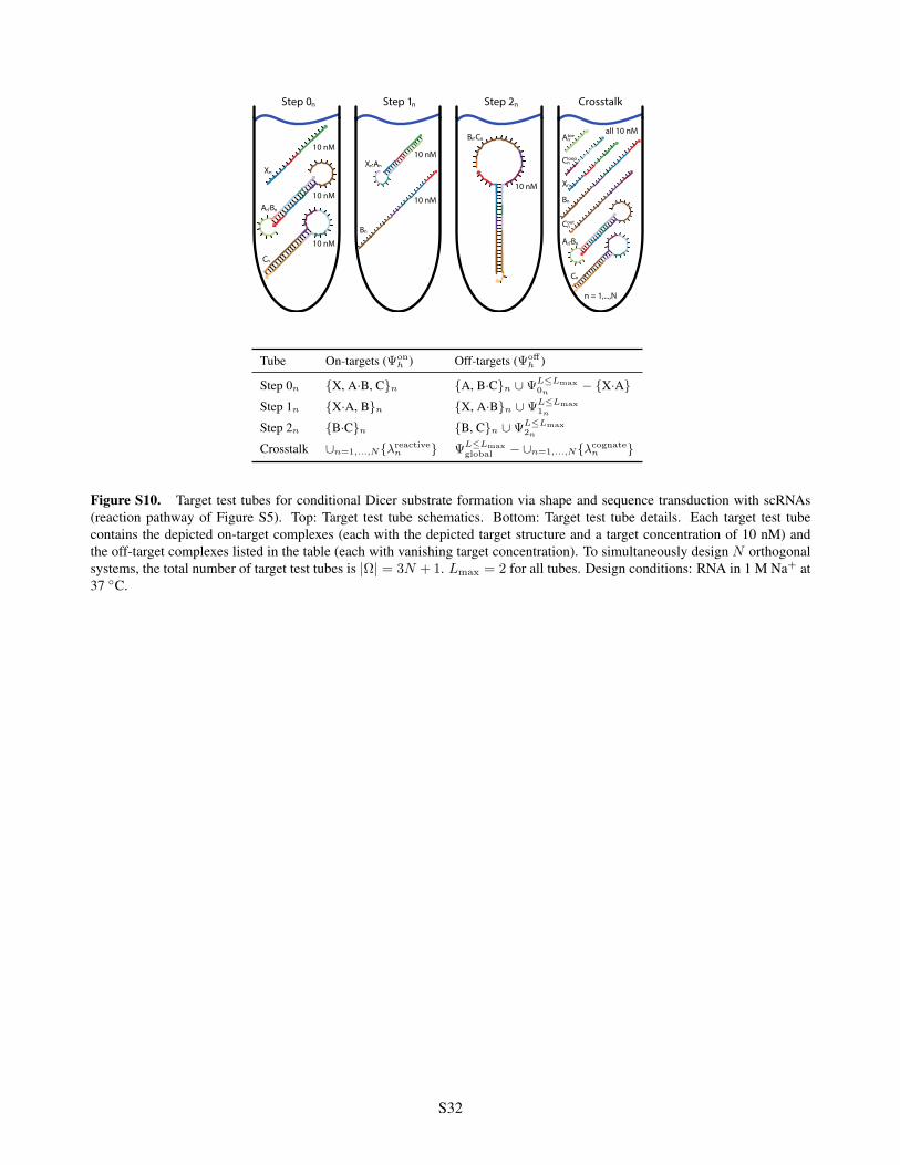
Step 0 Step 1 Step 2 Crosstalk
all 10 nM
10 nM 10 nM
10 nM
10 nM
B ·C Atoe
Cloop
Cout
C
A ·B
X
n = 1,...,N
B
X
C
n
n
n
n
n n
n
n
n
n
10 nMX ·An n
10 nM
Bn
n
A ·Bn n
n
n n n
Tube On-targets ( on
h ) Off-targets ( o↵
h )
Step 0n {X, A·B, C}n {A, B·C}n [
LLmax
0n− {X·A}
Step 1n {X·A, B}n {X, A·B}n [
LLmax
1n
Step 2n {B·C}n {B, C}n [
LLmax
2n
Crosstalk [n=1,...,N{λreactive
n }
LLmax
global
− [n=1,...,N{λcognate
n }
Figure S10. Target test tubes for conditional Dicer substrate formation via shape and sequence transduction with scRNAs(reaction pathway of Figure S5). Top: Target test tube schematics. Bottom: Target test tube details. Each target test tubecontains the depicted on-target complexes (each with the depicted target structure and a target concentration of 10 nM) andthe off-target complexes listed in the table (each with vanishing target concentration). To simultaneously design N orthogonalsystems, the total number of target test tubes is |⌦| = 3N + 1. L
max
= 2 for all tubes. Design conditions: RNA in 1 M Na+ at37 C.
S32
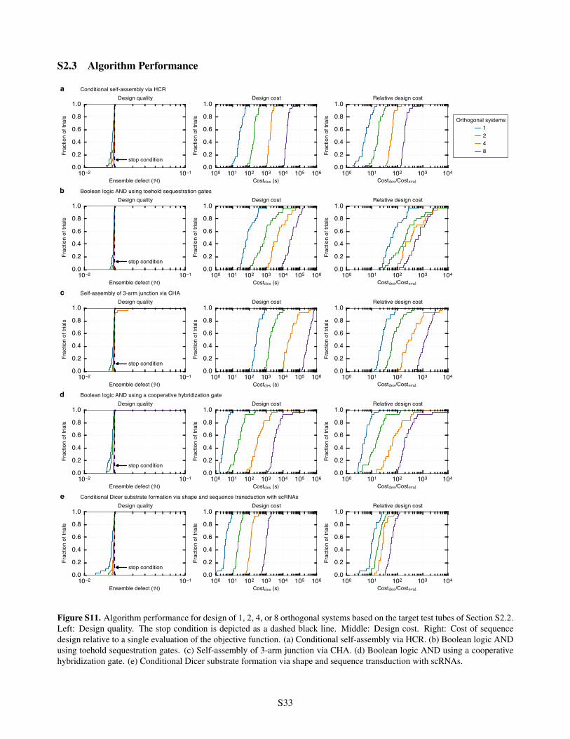
S2.3 Algorithm Performance
10−2 10−1
Ensemble defect (M)
0.0
0.2
0.4
0.6
0.8
1.0
Frac
tion
of tr
ials
stop condition
aDesign quality
100 101 102 103 104 105 106
Costdes (s)
0.0
0.2
0.4
0.6
0.8
1.0
Frac
tion
of tr
ials
Design cost
100 101 102 103 104
Costdes/Costeval
0.0
0.2
0.4
0.6
0.8
1.0
Frac
tion
of tr
ials
Relative design cost
10−2 10−1
Ensemble defect (M)
0.0
0.2
0.4
0.6
0.8
1.0
Frac
tion
of tr
ials
stop condition
bDesign quality
100 101 102 103 104 105 106
Costdes (s)
0.0
0.2
0.4
0.6
0.8
1.0Fr
actio
n of
tria
lsDesign cost
100 101 102 103 104
Costdes/Costeval
0.0
0.2
0.4
0.6
0.8
1.0
Frac
tion
of tr
ials
Relative design cost
10−2 10−1
Ensemble defect (M)
0.0
0.2
0.4
0.6
0.8
1.0
Frac
tion
of tr
ials
stop condition
cDesign quality
100 101 102 103 104 105 106
Costdes (s)
0.0
0.2
0.4
0.6
0.8
1.0
Frac
tion
of tr
ials
Design cost
100 101 102 103 104
Costdes/Costeval
0.0
0.2
0.4
0.6
0.8
1.0
Frac
tion
of tr
ials
Relative design cost
10−2 10−1
Ensemble defect (M)
0.0
0.2
0.4
0.6
0.8
1.0
Frac
tion
of tr
ials
stop condition
dDesign quality
100 101 102 103 104 105 106
Costdes (s)
0.0
0.2
0.4
0.6
0.8
1.0
Frac
tion
of tr
ials
Design cost
100 101 102 103 104
Costdes/Costeval
0.0
0.2
0.4
0.6
0.8
1.0
Frac
tion
of tr
ials
Relative design cost
10−2 10−1
Ensemble defect (M)
0.0
0.2
0.4
0.6
0.8
1.0
Frac
tion
of tr
ials
stop condition
eDesign quality
100 101 102 103 104 105 106
Costdes (s)
0.0
0.2
0.4
0.6
0.8
1.0
Frac
tion
of tr
ials
Design cost
100 101 102 103 104
Costdes/Costeval
0.0
0.2
0.4
0.6
0.8
1.0
Frac
tion
of tr
ials
Relative design cost
Conditional self-assembly via HCR
Boolean logic AND using toehold sequestration gates
Self-assembly of 3-arm junction via CHA
Boolean logic AND using a cooperative hybridization gate
Conditional Dicer substrate formation via shape and sequence transduction with scRNAs
Orthogonal systems1248
Figure S11. Algorithm performance for design of 1, 2, 4, or 8 orthogonal systems based on the target test tubes of Section S2.2.Left: Design quality. The stop condition is depicted as a dashed black line. Middle: Design cost. Right: Cost of sequencedesign relative to a single evaluation of the objective function. (a) Conditional self-assembly via HCR. (b) Boolean logic ANDusing toehold sequestration gates. (c) Self-assembly of 3-arm junction via CHA. (d) Boolean logic AND using a cooperativehybridization gate. (e) Conditional Dicer substrate formation via shape and sequence transduction with scRNAs.
S33
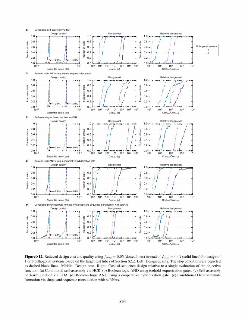
10−2 10−1
Ensemble defect (M)
0.0
0.2
0.4
0.6
0.8
1.0
Frac
tion
of tr
ials
2.0% 5.0%
aDesign quality
100 101 102 103 104 105 106
Costdes (s)
0.0
0.2
0.4
0.6
0.8
1.0
Frac
tion
of tr
ials
Design cost
100 101 102 103 104
Costdes/Costeval
0.0
0.2
0.4
0.6
0.8
1.0
Frac
tion
of tr
ials
Relative design cost
10−2 10−1
Ensemble defect (M)
0.0
0.2
0.4
0.6
0.8
1.0
Frac
tion
of tr
ials
2.0% 5.0%
bDesign quality
100 101 102 103 104 105 106
Costdes (s)
0.0
0.2
0.4
0.6
0.8
1.0Fr
actio
n of
tria
ls
Design cost
100 101 102 103 104
Costdes/Costeval
0.0
0.2
0.4
0.6
0.8
1.0
Frac
tion
of tr
ials
Relative design cost
10−2 10−1
Ensemble defect (M)
0.0
0.2
0.4
0.6
0.8
1.0
Frac
tion
of tr
ials
2.0% 5.0%
cDesign quality
100 101 102 103 104 105 106
Costdes (s)
0.0
0.2
0.4
0.6
0.8
1.0
Frac
tion
of tr
ials
Design cost
100 101 102 103 104
Costdes/Costeval
0.0
0.2
0.4
0.6
0.8
1.0
Frac
tion
of tr
ials
Relative design cost
10−2 10−1
Ensemble defect (M)
0.0
0.2
0.4
0.6
0.8
1.0
Frac
tion
of tr
ials
2.0% 5.0%
dDesign quality
100 101 102 103 104 105 106
Costdes (s)
0.0
0.2
0.4
0.6
0.8
1.0
Frac
tion
of tr
ials
Design cost
100 101 102 103 104
Costdes/Costeval
0.0
0.2
0.4
0.6
0.8
1.0
Frac
tion
of tr
ials
Relative design cost
10−2 10−1
Ensemble defect (M)
0.0
0.2
0.4
0.6
0.8
1.0
Frac
tion
of tr
ials
2.0% 5.0%
eDesign quality
100 101 102 103 104 105 106
Costdes (s)
0.0
0.2
0.4
0.6
0.8
1.0
Frac
tion
of tr
ials
Design cost
100 101 102 103 104
Costdes/Costeval
0.0
0.2
0.4
0.6
0.8
1.0
Frac
tion
of tr
ials
Relative design cost
Conditional self-assembly via HCR
Boolean logic AND using toehold sequestration gates
Self-assembly of 3-arm junction via CHA
Boolean logic AND using a cooperative hybridization gate
Conditional Dicer substrate formation via shape and sequence transduction with scRNAs
Orthogonal systems18
Figure S12. Reduced design cost and quality using fstop
= 0.05 (dotted lines) instead of fstop
= 0.02 (solid lines) for design of1 or 8 orthogonal systems based on the target test tubes of Section S2.2. Left: Design quality. The stop conditions are depictedas dashed black lines. Middle: Design cost. Right: Cost of sequence design relative to a single evaluation of the objectivefunction. (a) Conditional self-assembly via HCR. (b) Boolean logic AND using toehold sequestration gates. (c) Self-assemblyof 3-arm junction via CHA. (d) Boolean logic AND using a cooperative hybridization gate. (e) Conditional Dicer substrateformation via shape and sequence transduction with scRNAs.
S34

S2.4 Residual Defects
For each case study, the residual defect plots that follow display for each target test tube h 2 ⌦:
• The structural defect and concentration defect contributions of each on-target complex to the test tube ensem-ble defect, M
h
. The fact that bars are not depicted for off-targets does not mean that the defects associatedwith off-targets are neglected. By conservation of mass, nonzero off-target concentrations imply deficien-cies in on-target concentrations, and these on-target concentration defects are depicted in the bar graphs andincorporated in M
h
via (1) and (5).• The total structural defect and total concentration defect contributions of the tube to the multistate test tube
ensemble defect, M.
S35
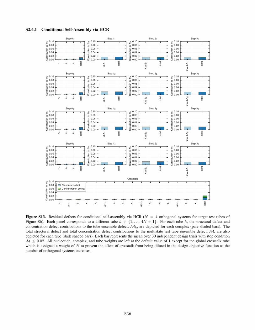
S2.4.1 Conditional Self-Assembly via HCR
A 1 B 1 X 1 tota
l0.000.020.040.060.080.10
Cont
ribut
ion
to M
h
Step 01
X⋅A 1 tota
l0.000.020.040.060.080.10
Cont
ribut
ion
to M
h
Step 11
X⋅A⋅
B 1 tota
l0.000.020.040.060.080.10
Cont
ribut
ion
to M
h
Step 21
X⋅A⋅
A⋅B 1
tota
l0.000.020.040.060.080.10
Cont
ribut
ion
to M
h
Step 31
A 2 B 2 X 2 tota
l0.000.020.040.060.080.10
Cont
ribut
ion
to M
h
Step 02
X⋅A 2 tota
l0.000.020.040.060.080.10
Cont
ribut
ion
to M
h
Step 12
X⋅A⋅
B 2 tota
l0.000.020.040.060.080.10
Cont
ribut
ion
to M
h
Step 22
X⋅A⋅
A⋅B 2
tota
l0.000.020.040.060.080.10
Cont
ribut
ion
to M
h
Step 32
A 3 B 3 X 3 tota
l0.000.020.040.060.080.10
Cont
ribut
ion
to M
h
Step 03
X⋅A 3 tota
l0.000.020.040.060.080.10
Cont
ribut
ion
to M
h
Step 13
X⋅A⋅
B 3 tota
l0.000.020.040.060.080.10
Cont
ribut
ion
to M
h
Step 23
X⋅A⋅
A⋅B 3
tota
l0.000.020.040.060.080.10
Cont
ribut
ion
to M
h
Step 33
A 4 B 4 X 4 tota
l0.000.020.040.060.080.10
Cont
ribut
ion
to M
h
Step 04
X⋅A 4 tota
l0.000.020.040.060.080.10
Cont
ribut
ion
to M
h
Step 14X⋅
A⋅B 4 tota
l0.000.020.040.060.080.10
Cont
ribut
ion
to M
h
Step 24
X⋅A⋅
A⋅B 4
tota
l0.000.020.040.060.080.10
Cont
ribut
ion
to M
h
Step 34
A 1
Aout
1 B 1 X 1 A 2
Aout
2 B 2 X 2 A 3
Aout
3 B 3 X 3 A 4
Aout
4 B 4 X 4 tota
l0.000.020.040.060.080.10
Cont
ribut
ion
to M
h
Crosstalk
Structural defectConcentration defect
Figure S13. Residual defects for conditional self-assembly via HCR (N = 4 orthogonal systems for target test tubes ofFigure S6). Each panel corresponds to a different tube h 2 {1, . . . , 4N + 1}. For each tube h, the structural defect andconcentration defect contributions to the tube ensemble defect, Mh, are depicted for each complex (pale shaded bars). Thetotal structural defect and total concentration defect contributions to the multistate test tube ensemble defect, M, are alsodepicted for each tube (dark shaded bars). Each bar represents the mean over 30 independent design trials with stop conditionM 0.02. All nucleotide, complex, and tube weights are left at the default value of 1 except for the global crosstalk tubewhich is assigned a weight of N to prevent the effect of crosstalk from being diluted in the design objective function as thenumber of orthogonal systems increases.
S36
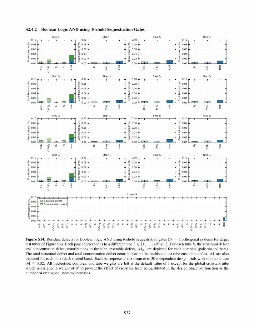
S2.4.2 Boolean Logic AND using Toehold Sequestration Gates
A⋅B 1
C⋅D⋅
E 1 X 1 Y 1 tota
l0.00
0.02
0.04
0.06
0.08
0.10
Cont
ribut
ion
to M
h
Step 01
B 1
X⋅A 1 tota
l0.00
0.02
0.04
0.06
0.08
0.10
Cont
ribut
ion
to M
h
Step 11
B⋅C
1
D⋅E 1 tota
l0.00
0.02
0.04
0.06
0.08
0.10
Cont
ribut
ion
to M
h
Step 21
E 1
Y⋅D
1
tota
l0.00
0.02
0.04
0.06
0.08
0.10
Cont
ribut
ion
to M
h
Step 31
A⋅B 2
C⋅D⋅
E 2 X 2 Y 2 tota
l0.00
0.02
0.04
0.06
0.08
0.10
Cont
ribut
ion
to M
h
Step 02
B 2
X⋅A 2 tota
l0.00
0.02
0.04
0.06
0.08
0.10Co
ntrib
utio
n to
Mh
Step 12
B⋅C
2
D⋅E 2 tota
l0.00
0.02
0.04
0.06
0.08
0.10
Cont
ribut
ion
to M
h
Step 22
E 2
Y⋅D
2
tota
l0.00
0.02
0.04
0.06
0.08
0.10
Cont
ribut
ion
to M
h
Step 32
A⋅B 3
C⋅D⋅
E 3 X 3 Y 3 tota
l0.00
0.02
0.04
0.06
0.08
0.10
Cont
ribut
ion
to M
h
Step 03
B 3
X⋅A 3 tota
l0.00
0.02
0.04
0.06
0.08
0.10
Cont
ribut
ion
to M
h
Step 13
B⋅C
3
D⋅E 3 tota
l0.00
0.02
0.04
0.06
0.08
0.10
Cont
ribut
ion
to M
h
Step 23
E 3
Y⋅D
3
tota
l0.00
0.02
0.04
0.06
0.08
0.10
Cont
ribut
ion
to M
h
Step 33
A⋅B 4
C⋅D⋅
E 4 X 4 Y 4 tota
l0.00
0.02
0.04
0.06
0.08
0.10
Cont
ribut
ion
to M
h
Step 04
B 4
X⋅A 4 tota
l0.00
0.02
0.04
0.06
0.08
0.10
Cont
ribut
ion
to M
h
Step 14
B⋅C
4
D⋅E 4 tota
l0.00
0.02
0.04
0.06
0.08
0.10
Cont
ribut
ion
to M
h
Step 24
E 4
Y⋅D
4
tota
l0.00
0.02
0.04
0.06
0.08
0.10
Cont
ribut
ion
to M
h
Step 34
A⋅B 1
Atoe
1 B 1C⋅
Dou
t 1
Cto
e 1
D⋅E 1
Dou
t 1 E 1 X 1 Y 1A⋅
B 2At
oe2 B 2
C⋅D
out 2
Cto
e 2
D⋅E 2
Dou
t 2 E 2 X 2 Y 2A⋅
B 3At
oe3 B 3
C⋅D
out 3
Cto
e 3
D⋅E 3
Dou
t 3 E 3 X 3 Y 3A⋅
B 4At
oe4 B 4
C⋅D
out 4
Cto
e 4
D⋅E 4
Dou
t 4 E 4 X 4 Y 4 tota
l0.00
0.02
0.04
0.06
0.08
0.10
Cont
ribut
ion
to M
h
Crosstalk
Structural defectConcentration defect
Figure S14. Residual defects for Boolean logic AND using toehold sequestration gates (N = 4 orthogonal systems for targettest tubes of Figure S7). Each panel corresponds to a different tube h 2 {1, . . . , 4N +1}. For each tube h, the structural defectand concentration defect contributions to the tube ensemble defect, Mh, are depicted for each complex (pale shaded bars).The total structural defect and total concentration defect contributions to the multistate test tube ensemble defect, M, are alsodepicted for each tube (dark shaded bars). Each bar represents the mean over 30 independent design trials with stop conditionM 0.02. All nucleotide, complex, and tube weights are left at the default value of 1 except for the global crosstalk tubewhich is assigned a weight of N to prevent the effect of crosstalk from being diluted in the design objective function as thenumber of orthogonal systems increases.
S37
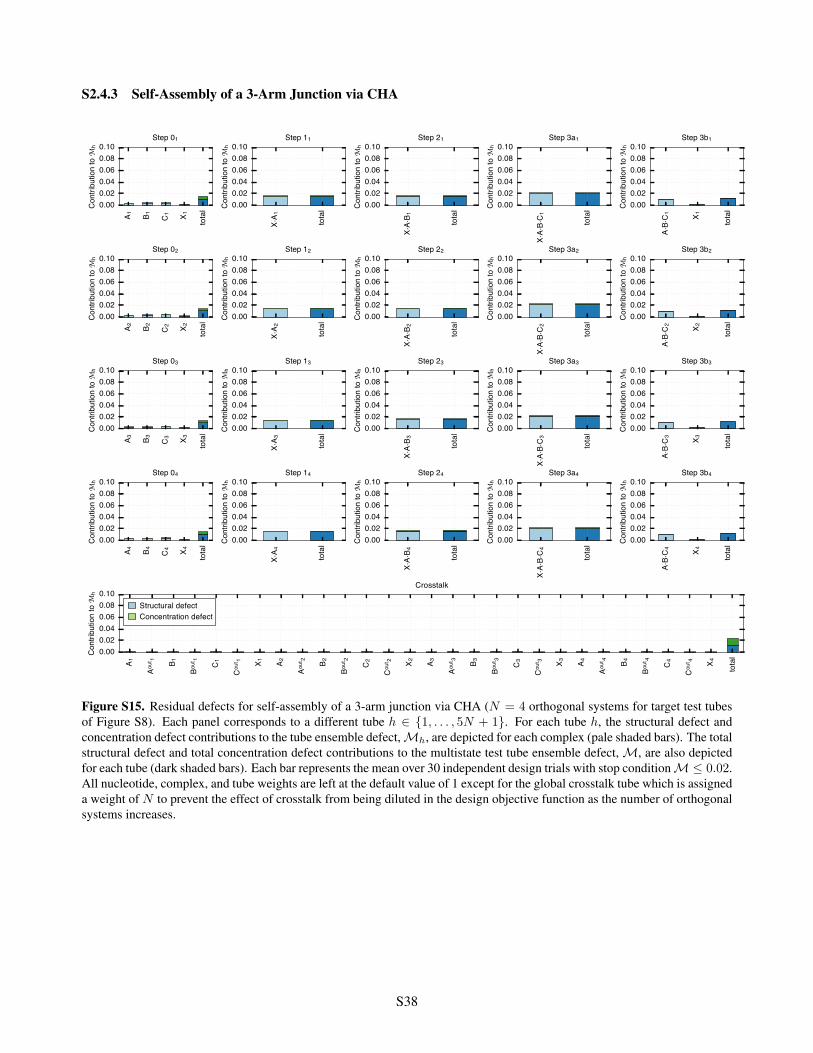
S2.4.3 Self-Assembly of a 3-Arm Junction via CHA
A 1 B 1 C1 X 1 to
tal0.00
0.020.040.060.080.10
Cont
ribut
ion
to M
h
Step 01
X⋅A 1 tota
l0.000.020.040.060.080.10
Cont
ribut
ion
to M
h
Step 11
X⋅A⋅
B 1 tota
l0.000.020.040.060.080.10
Cont
ribut
ion
to M
h
Step 21
X⋅A⋅
B⋅C
1
tota
l0.000.020.040.060.080.10
Cont
ribut
ion
to M
h
Step 3a1
A⋅B⋅
C1 X 1 to
tal0.00
0.020.040.060.080.10
Cont
ribut
ion
to M
h
Step 3b1
A 2 B 2 C2 X 2 to
tal0.00
0.020.040.060.080.10
Cont
ribut
ion
to M
h
Step 02
X⋅A 2 tota
l0.000.020.040.060.080.10
Cont
ribut
ion
to M
h
Step 12
X⋅A⋅
B 2 tota
l0.000.020.040.060.080.10
Cont
ribut
ion
to M
h
Step 22
X⋅A⋅
B⋅C
2
tota
l0.000.020.040.060.080.10
Cont
ribut
ion
to M
h
Step 3a2
A⋅B⋅
C2 X 2 to
tal0.00
0.020.040.060.080.10
Cont
ribut
ion
to M
h
Step 3b2
A 3 B 3 C3 X 3 to
tal0.00
0.020.040.060.080.10
Cont
ribut
ion
to M
h
Step 03
X⋅A 3 tota
l0.000.020.040.060.080.10
Cont
ribut
ion
to M
h
Step 13
X⋅A⋅
B 3 tota
l0.000.020.040.060.080.10
Cont
ribut
ion
to M
hStep 23
X⋅A⋅
B⋅C
3
tota
l0.000.020.040.060.080.10
Cont
ribut
ion
to M
h
Step 3a3
A⋅B⋅
C3 X 3 to
tal0.00
0.020.040.060.080.10
Cont
ribut
ion
to M
h
Step 3b3
A 4 B 4 C4 X 4 to
tal0.00
0.020.040.060.080.10
Cont
ribut
ion
to M
h
Step 04
X⋅A 4 tota
l0.000.020.040.060.080.10
Cont
ribut
ion
to M
h
Step 14
X⋅A⋅
B 4 tota
l0.000.020.040.060.080.10
Cont
ribut
ion
to M
h
Step 24
X⋅A⋅
B⋅C
4
tota
l0.000.020.040.060.080.10
Cont
ribut
ion
to M
h
Step 3a4
A⋅B⋅
C4 X 4 to
tal0.00
0.020.040.060.080.10
Cont
ribut
ion
to M
h
Step 3b4
A 1
Aout
1 B 1
Bout
1
C1
Cou
t 1 X 1 A 2
Aout
2 B 2
Bout
2
C2
Cou
t 2 X 2 A 3
Aout
3 B 3
Bout
3
C3
Cou
t 3 X 3 A 4
Aout
4 B 4
Bout
4
C4
Cou
t 4 X 4 tota
l0.000.020.040.060.080.10
Cont
ribut
ion
to M
h
Crosstalk
Structural defectConcentration defect
Figure S15. Residual defects for self-assembly of a 3-arm junction via CHA (N = 4 orthogonal systems for target test tubesof Figure S8). Each panel corresponds to a different tube h 2 {1, . . . , 5N + 1}. For each tube h, the structural defect andconcentration defect contributions to the tube ensemble defect, Mh, are depicted for each complex (pale shaded bars). The totalstructural defect and total concentration defect contributions to the multistate test tube ensemble defect, M, are also depictedfor each tube (dark shaded bars). Each bar represents the mean over 30 independent design trials with stop condition M 0.02.All nucleotide, complex, and tube weights are left at the default value of 1 except for the global crosstalk tube which is assigneda weight of N to prevent the effect of crosstalk from being diluted in the design objective function as the number of orthogonalsystems increases.
S38

S2.4.4 Boolean Logic AND using a Cooperative Hybridization Gate
A⋅B 1 X 1 Y 1 tota
l0.00
0.02
0.04
0.06
0.08
0.10
Cont
ribut
ion
to M
h
Step 01
B 1
Y⋅A⋅
X 1 tota
l0.00
0.02
0.04
0.06
0.08
0.10
Cont
ribut
ion
to M
h
Step 11
A⋅B 2 X 2 Y 2 tota
l0.00
0.02
0.04
0.06
0.08
0.10
Cont
ribut
ion
to M
h
Step 02
B 2
Y⋅A⋅
X 2 tota
l0.00
0.02
0.04
0.06
0.08
0.10
Cont
ribut
ion
to M
h
Step 12
A⋅B 3 X 3 Y 3 tota
l0.00
0.02
0.04
0.06
0.08
0.10
Cont
ribut
ion
to M
h
Step 03
B 3
Y⋅A⋅
X 3 tota
l0.00
0.02
0.04
0.06
0.08
0.10Co
ntrib
utio
n to
Mh
Step 13
A⋅B 4 X 4 Y 4 tota
l0.00
0.02
0.04
0.06
0.08
0.10
Cont
ribut
ion
to M
h
Step 04
B 4
Y⋅A⋅
X 4 tota
l0.00
0.02
0.04
0.06
0.08
0.10
Cont
ribut
ion
to M
h
Step 14
Alef
t ⋅Ble
ft 1
Alef
t−to
e 1
Arig
ht⋅B
right
1
Arig
ht−
toe 1
B 1 X 1 Y 1Al
eft ⋅B
left 2
Alef
t−to
e 2
Arig
ht⋅B
right
2
Arig
ht−
toe 2
B 2 X 2 Y 2Al
eft ⋅B
left 3
Alef
t−to
e 3
Arig
ht⋅B
right
3
Arig
ht−
toe 3
B 3 X 3 Y 3Al
eft ⋅B
left 4
Alef
t−to
e 4
Arig
ht⋅B
right
4
Arig
ht−
toe 4
B 4 X 4 Y 4 tota
l0.00
0.02
0.04
0.06
0.08
0.10
Cont
ribut
ion
to M
h
Crosstalk
Structural defectConcentration defect
Figure S16. Residual defects for Boolean logic AND using a cooperative hybridization gate (N = 4 orthogonal systems fortarget test tubes of Figure S9). Each panel corresponds to a different tube h 2 {1, . . . , 2N + 1}. For each tube h, the structuraldefect and concentration defect contributions to the tube ensemble defect, Mh, are depicted for each complex (pale shadedbars). The total structural defect and total concentration defect contributions to the multistate test tube ensemble defect, M,are also depicted for each tube (dark shaded bars). Each bar represents the mean over 30 independent design trials with stopcondition M 0.02. All nucleotide, complex, and tube weights are left at the default value of 1 except for the global crosstalktube which is assigned a weight of N to prevent the effect of crosstalk from being diluted in the design objective function asthe number of orthogonal systems increases.
S39
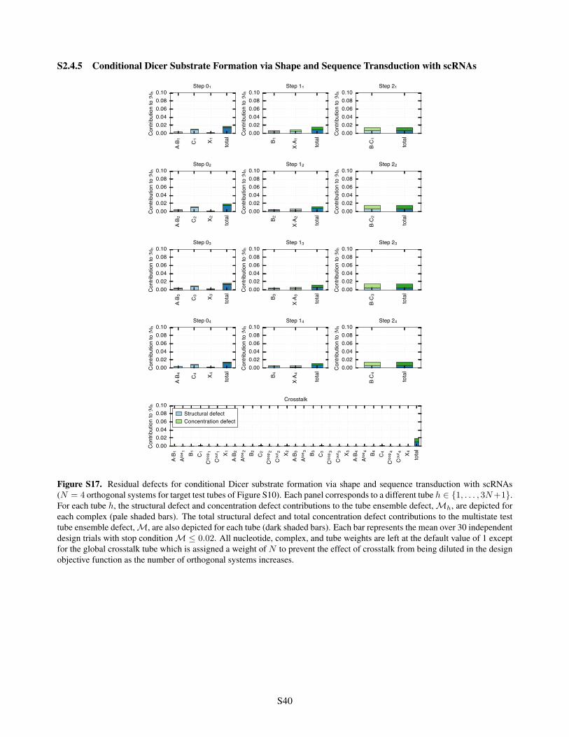
S2.4.5 Conditional Dicer Substrate Formation via Shape and Sequence Transduction with scRNAs
A⋅B 1 C
1 X 1 tota
l0.000.020.040.060.080.10
Cont
ribut
ion
to M
h
Step 01
B 1
X⋅A 1 tota
l0.000.020.040.060.080.10
Cont
ribut
ion
to M
h
Step 11
B⋅C
1
tota
l0.000.020.040.060.080.10
Cont
ribut
ion
to M
h
Step 21
A⋅B 2 C
2 X 2 tota
l0.000.020.040.060.080.10
Cont
ribut
ion
to M
h
Step 02
B 2
X⋅A 2 tota
l0.000.020.040.060.080.10
Cont
ribut
ion
to M
h
Step 12
B⋅C
2
tota
l0.000.020.040.060.080.10
Cont
ribut
ion
to M
h
Step 22
A⋅B 3 C
3 X 3 tota
l0.000.020.040.060.080.10
Cont
ribut
ion
to M
h
Step 03
B 3
X⋅A 3 tota
l0.000.020.040.060.080.10
Cont
ribut
ion
to M
hStep 13
B⋅C
3
tota
l0.000.020.040.060.080.10
Cont
ribut
ion
to M
h
Step 23
A⋅B 4 C
4 X 4 tota
l0.000.020.040.060.080.10
Cont
ribut
ion
to M
h
Step 04
B 4
X⋅A 4 tota
l0.000.020.040.060.080.10
Cont
ribut
ion
to M
h
Step 14
B⋅C
4
tota
l0.000.020.040.060.080.10
Cont
ribut
ion
to M
h
Step 24
A⋅B 1
Atoe
1 B 1 C1
Clo
op1
Cou
t 1 X 1A⋅
B 2At
oe2 B 2 C2
Clo
op2
Cou
t 2 X 2A⋅
B 3At
oe3 B 3 C3
Clo
op3
Cou
t 3 X 3A⋅
B 4At
oe4 B 4 C4
Clo
op4
Cou
t 4 X 4 tota
l0.000.020.040.060.080.10
Cont
ribut
ion
to M
h
Crosstalk
Structural defectConcentration defect
Figure S17. Residual defects for conditional Dicer substrate formation via shape and sequence transduction with scRNAs(N = 4 orthogonal systems for target test tubes of Figure S10). Each panel corresponds to a different tube h 2 {1, . . . , 3N+1}.For each tube h, the structural defect and concentration defect contributions to the tube ensemble defect, Mh, are depicted foreach complex (pale shaded bars). The total structural defect and total concentration defect contributions to the multistate testtube ensemble defect, M, are also depicted for each tube (dark shaded bars). Each bar represents the mean over 30 independentdesign trials with stop condition M 0.02. All nucleotide, complex, and tube weights are left at the default value of 1 exceptfor the global crosstalk tube which is assigned a weight of N to prevent the effect of crosstalk from being diluted in the designobjective function as the number of orthogonal systems increases.
S40
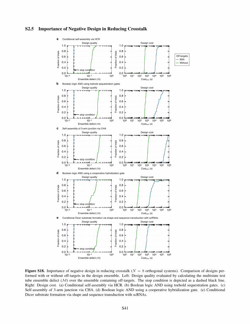
S2.5 Importance of Negative Design in Reducing Crosstalk
10−2 10−1 100
Ensemble defect (M)
0.0
0.2
0.4
0.6
0.8
1.0
Frac
tion
of tr
ials
stop condition
aDesign quality
100 101 102 103 104 105 106
Costdes (s)
0.0
0.2
0.4
0.6
0.8
1.0
Frac
tion
of tr
ials
Design cost
10−2 10−1 100
Ensemble defect (M)
0.0
0.2
0.4
0.6
0.8
1.0
Frac
tion
of tr
ials
stop condition
bDesign quality
100 101 102 103 104 105 106
Costdes (s)
0.0
0.2
0.4
0.6
0.8
1.0
Frac
tion
of tr
ials
Design cost
10−2 10−1 100
Ensemble defect (M)
0.0
0.2
0.4
0.6
0.8
1.0
Frac
tion
of tr
ials
stop condition
cDesign quality
100 101 102 103 104 105 106
Costdes (s)
0.0
0.2
0.4
0.6
0.8
1.0
Frac
tion
of tr
ials
Design cost
10−2 10−1 100
Ensemble defect (M)
0.0
0.2
0.4
0.6
0.8
1.0
Frac
tion
of tr
ials
stop condition
dDesign quality
100 101 102 103 104 105 106
Costdes (s)
0.0
0.2
0.4
0.6
0.8
1.0
Frac
tion
of tr
ials
Design cost
10−2 10−1 100
Ensemble defect (M)
0.0
0.2
0.4
0.6
0.8
1.0
Frac
tion
of tr
ials
stop condition
eDesign quality
100 101 102 103 104 105 106
Costdes (s)
0.0
0.2
0.4
0.6
0.8
1.0
Frac
tion
of tr
ials
Design cost
Conditional self-assembly via HCR
Boolean logic AND using toehold sequestration gates
Self-assembly of 3-arm junction via CHA
Boolean logic AND using a cooperative hybridization gate
Conditional Dicer substrate formation via shape and sequence transduction with scRNAs
Off-targetsWithWithout
Figure S18. Importance of negative design in reducing crosstalk (N = 8 orthogonal systems). Comparison of designs per-formed with or without off-targets in the design ensemble. Left: Design quality evaluated by calculating the multistate testtube ensemble defect (M) over the ensemble containing off-targets. The stop condition is depicted as a dashed black line.Right: Design cost. (a) Conditional self-assembly via HCR. (b) Boolean logic AND using toehold sequestration gates. (c)Self-assembly of 3-arm junction via CHA. (d) Boolean logic AND using a cooperative hybridization gate. (e) ConditionalDicer substrate formation via shape and sequence transduction with scRNAs.
S41
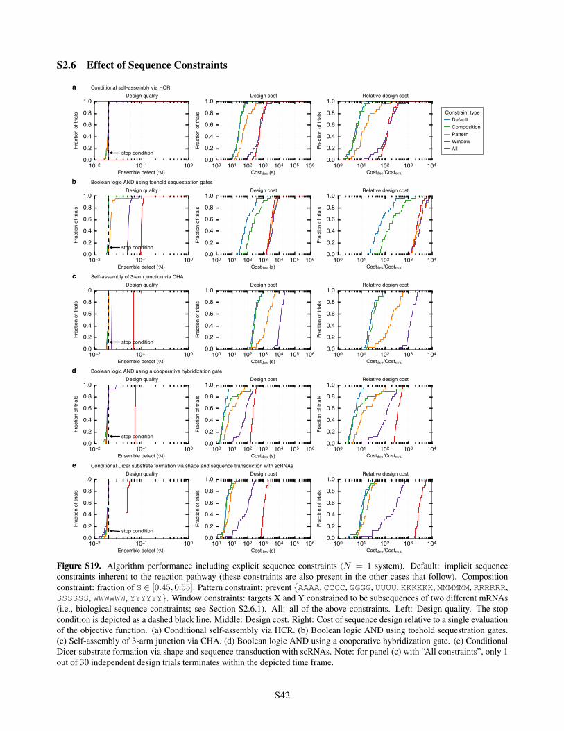
S2.6 Effect of Sequence Constraints
10−2 10−1 100
Ensemble defect (M)
0.0
0.2
0.4
0.6
0.8
1.0
Frac
tion
of tr
ials
stop condition
aDesign quality
100 101 102 103 104 105 106
Costdes (s)
0.0
0.2
0.4
0.6
0.8
1.0
Frac
tion
of tr
ials
Design cost
100 101 102 103 104
Costdes/Costeval
0.0
0.2
0.4
0.6
0.8
1.0
Frac
tion
of tr
ials
Relative design cost
10−2 10−1 100
Ensemble defect (M)
0.0
0.2
0.4
0.6
0.8
1.0
Frac
tion
of tr
ials
stop condition
bDesign quality
100 101 102 103 104 105 106
Costdes (s)
0.0
0.2
0.4
0.6
0.8
1.0Fr
actio
n of
tria
lsDesign cost
100 101 102 103 104
Costdes/Costeval
0.0
0.2
0.4
0.6
0.8
1.0
Frac
tion
of tr
ials
Relative design cost
10−2 10−1 100
Ensemble defect (M)
0.0
0.2
0.4
0.6
0.8
1.0
Frac
tion
of tr
ials
stop condition
cDesign quality
100 101 102 103 104 105 106
Costdes (s)
0.0
0.2
0.4
0.6
0.8
1.0
Frac
tion
of tr
ials
Design cost
100 101 102 103 104
Costdes/Costeval
0.0
0.2
0.4
0.6
0.8
1.0
Frac
tion
of tr
ials
Relative design cost
10−2 10−1 100
Ensemble defect (M)
0.0
0.2
0.4
0.6
0.8
1.0
Frac
tion
of tr
ials
stop condition
dDesign quality
100 101 102 103 104 105 106
Costdes (s)
0.0
0.2
0.4
0.6
0.8
1.0
Frac
tion
of tr
ials
Design cost
100 101 102 103 104
Costdes/Costeval
0.0
0.2
0.4
0.6
0.8
1.0
Frac
tion
of tr
ials
Relative design cost
10−2 10−1 100
Ensemble defect (M)
0.0
0.2
0.4
0.6
0.8
1.0
Frac
tion
of tr
ials
stop condition
eDesign quality
100 101 102 103 104 105 106
Costdes (s)
0.0
0.2
0.4
0.6
0.8
1.0
Frac
tion
of tr
ials
Design cost
100 101 102 103 104
Costdes/Costeval
0.0
0.2
0.4
0.6
0.8
1.0
Frac
tion
of tr
ials
Relative design cost
Conditional self-assembly via HCR
Boolean logic AND using toehold sequestration gates
Self-assembly of 3-arm junction via CHA
Boolean logic AND using a cooperative hybridization gate
Conditional Dicer substrate formation via shape and sequence transduction with scRNAs
Constraint typeDefaultCompositionPatternWindowAll
Figure S19. Algorithm performance including explicit sequence constraints (N = 1 system). Default: implicit sequenceconstraints inherent to the reaction pathway (these constraints are also present in the other cases that follow). Compositionconstraint: fraction of S 2 [0.45, 0.55]. Pattern constraint: prevent {AAAA, CCCC, GGGG, UUUU, KKKKKK, MMMMMM, RRRRRR,SSSSSS, WWWWWW, YYYYYY}. Window constraints: targets X and Y constrained to be subsequences of two different mRNAs(i.e., biological sequence constraints; see Section S2.6.1). All: all of the above constraints. Left: Design quality. The stopcondition is depicted as a dashed black line. Middle: Design cost. Right: Cost of sequence design relative to a single evaluationof the objective function. (a) Conditional self-assembly via HCR. (b) Boolean logic AND using toehold sequestration gates.(c) Self-assembly of 3-arm junction via CHA. (d) Boolean logic AND using a cooperative hybridization gate. (e) ConditionalDicer substrate formation via shape and sequence transduction with scRNAs. Note: for panel (c) with “All constraints”, only 1out of 30 independent design trials terminates within the depicted time frame.
S42

S2.6.1 mRNA Sequences used for Window Constraints
The window constraints used for the studies of Figures 5 and S19 constrain targets X and Y to be subsequences ofzebrafish mRNA sequences tpm3 (2175 nt) and desma (1798 nt), respectively. Zebrafish mRNA sequences wereobtained from the National Center for Biotechnology Information (NCBI).61 Sequences are listed below 5
0 to 3
0.Table S3 lists the sequence domains constrained by window constraints for each reaction pathway, the number ofcandidate windows within each mRNA, and the number of these candidate windows that also satisfy the compositionconstraints, the pattern prevention constraints, or both the composition and pattern prevention constraints.
mRNA: tropomyosin 3 (tpm3)Sequence: gAACACUAUUAgCUAUUUgUAgUACUCUAAAgAggACUgCAgAACgCAUCgCAgUAgUggUgAAAAgCCgUgCgUgCgCgUgAAACAUCUgAUCC
UCACgUUACUUCCACUCgCUCUgCgUUUgACUUgUUggCggggCgUUggUgCCUUggACUUUUUUUUCCUCCUUCUCUUCUUCgCggCUCggUCCACUACgCUgC
UCgAgAggAAUCUgCUUUAUUCgACCACACUACUCCUAAAgUAACACAUUAAAAUggCCggAUCAAACAgCAUCgAUgCAgUUAAgAgAAAAAUCAAAgUUUUAC
AACAgCAAgCAgAUgAggCAgAAgAAAgAgCCgAgAUUUUgCAgAgACAggUCgAggAggAgAAgCgUgCCAgggAgCAggCUgAggCAgAggUggCUUCUCUgA
ACAggCgUAUCCAgCUggUUgAggAggAgUUggAUCgUgCUCAggAgAgACUggCCACAgCCCUgCAAAAgCUggAggAAgCCgAgAAggCCgCAgAUgAgAgCg
AgAgAgggAUgAAggUgAUUgAgAACAgggCUCUgAAggAUgAggAgAAgAUggAgCUgCAggAgAUCCAgCUUAAggAggCCAAgCACAUUgCUgAggAggCUg
ACCgCAAAUAUgAAgAggUggCUCgUAAgCUggUgAUCgUUgAgggAgAgUUggAgCgUACAgAggAgAgAgCAgAgCUUgCAgAgAgCCAUgUCAAgCAgAUgg
AggAggAgCUgAgAgCUCUUgACCAgACACUgAAgACUCUUCAggCCUCAgAggAgAAgUAUUCCCAgAAggAggACAAgUAUgAggAAgAAAUCAAgAUCCUCA
CUgAUAAgCUgAAggAggCUgAgACCCgUgCAgAgUUUgCUgAgAggUCUgUggCCAAACUggAgAAAACCAUUgAUgAUUUggAAgAgAAACUgAgAgAUgCUA
AAgAggAgAACAUCAAgAUCCAUgCUACUUUggACCAgACCCUgAgCgAgCUCAAUAgUUUCUAAAgAAgACCUggAgCAgAAAAAAggCCUUUUCUUCCCUUCU
UgACUCCCUCAUCUCAUUUUggUUUCUUUgUCUCUgCACAUCUgAUUCUCCCCCUUUUUUUUUCUUCUCUUCUUCUgCUggAggAUAAgCUCACCAAgCCAACCA
gCAAAAAUgUggUgCCUCUCAAUUUUUCCAAACUACUAUUCCAAgUgAUUUgAgAAAUgAUCUACUACgAUACUCCUCAAgAgUCAAAUgUUgACCUCggggAgC
CUUUUUUggUAUUgCUCCAUgAUCAgAgCUUUACgAgCUAgUgUUUUUUCUgCAUAUCAgCCCAAACUCUCAAUgAUAAUUUUACUggAggCUgAUUUUUgUAAA
AUUUUgUgCCAUAAAAgCCUUgUUggCUUgUCUCUUgCUUggCUUUAgAUCAUUCUCAAgCCAUUUUUUUCCUgCUgUUgCUCUgACACAggUUgUUUUUgCUgg
UCUUgUUggUgCCUgAUCCACUgCUAUCCUUUUCACACCUCUUUUUUUUUUUUCUUCAUCCUgCACAAgUUUCUgCUgCCUgUUAgUCggCAUCACCggUUUUgg
gACCAAAACCACAUCAUgUggUCUgUAACAgUAUgCACAACCAUgCCgUgAggACCAAAUUUgUUUUAUUAUUgUUAUUAUUAUUAAAAgCCUUUgCUUCCAUUC
ggAgUUUgUUUUUUUgAgUAAUAUAUgUAUUCAUUgUUUgggUCgAAUCCCCUUgCUUUUUUAACACAAAUgUUUUgCAAACCACUAUUUgAAAUggUgCACUgU
UAUgggCUUAUggUgAgCAgAUgAggCCAAgUCAUggUUUCUUCAUUAUAAUUUUCUUUUCAUUUgCUUUAAAgAgCCAUAUUCUACCCAgggAAgAAAggUUgA
AgUUgUUUUgUUUUUUUACCgUgAgUUCAAAgCAgUggCACUgCCAgAUUUAAAAggUUCAAAAgCCgUgCAgAUCUAAAAUAUgUAUUAUgAACACAgUAAUgg
gAgCgAAUUgUAACACUUAAUAgUAUACAAAUUUAAgAAACAggggUgAACACAUAgUUUUAACUggAAAAAgCCCACAAUgAUgUgUAAUCACUUUgUUACUgU
CUgUAUCUUgUgUAAUgAUACCUAAAUUCUUUUUUUAAAUAAAAACCAUgAUUUUUACUgUCACUgAAAAAAAAAAAAAAAAAAA
mRNA: desmin a (desma)Sequence: CAUUUACACAgCgUACAAACCCAACAggCCCAgUCAUgAgCACgAAAUAUUCAgCCUCCgCCgAgUCggCgUCCUCUUACCgCCgCACCUUUggC
UCAggUUUgggCUCCUCUAUUUUCgCCggCCACggUUCCUCAggUUCCUCUggCUCCUCAAgACUgACCUCCAgAgUUUACgAggUgACCAAgAgCUCCgCUUCU
CCCCAUUUUUCCAgCCACCgUgCgUCCggCUCUUUCggAggUggCUCggUggUCCgUUCCUACgCUggCCUUggUgAgAAgCUggAUUUCAAUCUggCUgAUgCC
AUAAACCAggACUUCCUCAACACgCgUACUAAUgAgAAggCCgAgCUCCAgCACCUCAAUgACCgCUUCgCCAgCUACAUCgAgAAggUgCgCUUCCUCgAgCAg
CAgAACUCUgCCCUgACggUggAgAUUgAgCgUCUgCggggUCgCgAgCCCACCCgUAUUgCAgAgCUgUACgAggAggAgAUgAgAgAgCUgCgCggACAggUg
gAggCACUgACCAAUCAgAgAUCCCgUgUggAgAUCgAgAgggACAACCUAgUCgAUgACCUACAgAAACUAAAgCUCAgACUUCAAgAggAgAUCCACCAgAAA
gAggAAgCUgAAAACAACCUUUCUgCUUUCAgAgCUgAUgUCgAUgCUgCCACUCUggCCAggCUggACCUggAAAgACgUAUCgAgggUCUUCACgAAgAgAUU
gCAUUCCUCAggAAgAUUCAUgAggAggAgAUCCgUgAgCUgCAgAACCAgAUgCAggAgAgUCAggUgCAgAUCCAAAUggACAUgUCCAAACCAgACCUgACU
gCggCCCUCAgAgACAUUCgCCUgCAgUACgAggCUAUCgCUgCCAAgAAUAUCAgCgAggCCgAggACUggUAUAAgUCUAAggUUUCAgAUUUgAACCAggCA
gUgAACAAgAAUAACgAggCUCUCAgAgAAgCCAAgCAggAgACCAUgCAgUUCCgUCACCAgCUCCAgUCCUACACCUgCgAgAUUgACUCUCUCAAgggCACC
AAUgAgUCUCUgAggAggCAAAUgAgUgAgAUggAggAgCggCUgggACgUgAggCCggUggUUAUCAggACACUAUCgCCCgUCUCgAggCUgAgAUCgCAAAA
AUgAAAgACgAgAUggCCCgCCACCUCCgCgAgUACCAggAUCUgCUgAAUgUgAAgAUggCUCUggAUgUggAgAUCgCCACCUACAggAAgCUUUUggAAggA
gAggAgAgCAggAUCUCgCUgCCCgUgCAgUCCUUUUCAUCCCUgAgUUUCAgAgAgAgCAgUCCAgAgCAgCACCACCACCAgCAgCAgCAACCACAACgCUCA
UCUgAAgUCCACUCCAAgAAAACAgUCCUgAUCAAgACCAUCgAgACCCgCgAUggCgAggUCgUCAgCgAgUCCACACAgCACCAgCAggACgUCAUgUAAAgC
UUgAgAAACAgAUCgAgUUUCACAgAAUgCCUUgCAUUUUCACUgAUggCCUCAggCUUUUUUAAgCACACACCCAgUAUUgCCgUgACCCAUUACCgCAUgUgg
AUgACgCAUggAgACAAAAggAAAgUgAgCUgAAAAACCAgAgggAggAAAAgUggAAUggUgUgAUgCUgAgCgUUCAgAAAgUggCCAgAUgAgCUCAgAgUU
UCUgAUUUAAUgAAUgUAUgUgUgCgUgUgUgUgUggUUgggUCAUAUCUgAgACACUgUUCCACAgCAACAAAAACAAUAAAAUUCACUgUAUUUUCUCCUAAA
AAAAAAAAAAAAAAAAAAAAAAA
S43
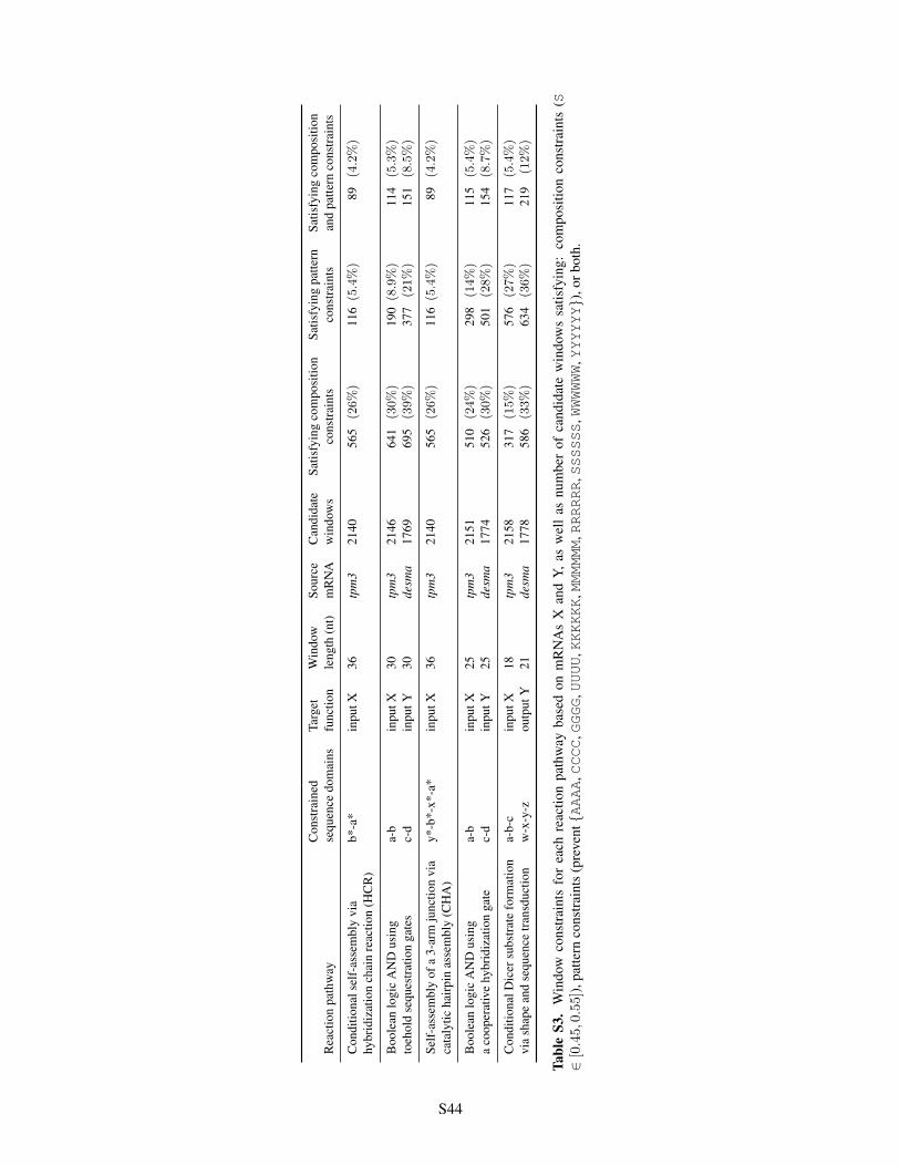
Con
stra
ined
Targ
etW
indo
wSo
urce
Can
dida
teSa
tisfy
ing
com
posi
tion
Satis
fyin
gpa
ttern
Satis
fyin
gco
mpo
sitio
nR
eact
ion
path
way
sequ
ence
dom
ains
func
tion
leng
th(n
t)m
RN
Aw
indo
ws
cons
trai
nts
cons
trai
nts
and
patte
rnco
nstr
aint
s
Con
ditio
nals
elf-
asse
mbl
yvi
ab*
-a*
inpu
tX36
tpm
321
4056
5(26%)
116(5.4%)
89(4.2%)
hybr
idiz
atio
nch
ain
reac
tion
(HC
R)
Boo
lean
logi
cA
ND
usin
ga-
bin
putX
30tp
m3
2146
641
(30%)
190(8.9%)
114
(5.3%)
toeh
old
sequ
estr
atio
nga
tes
c-d
inpu
tY30
desm
a17
6969
5(39%)
377
(21%)
151
(8.5%)
Self
-ass
embl
yof
a3-
arm
junc
tion
via
y*-b
*-x*
-a*
inpu
tX36
tpm
321
4056
5(26%)
116(5.4%)
89(4.2%)
cata
lytic
hair
pin
asse
mbl
y(C
HA
)
Boo
lean
logi
cA
ND
usin
ga-
bin
putX
25tp
m3
2151
510
(24%)
298
(14%)
115
(5.4%)
aco
oper
ativ
ehy
brid
izat
ion
gate
c-d
inpu
tY25
desm
a17
7452
6(30%)
501
(28%)
154
(8.7%)
Con
ditio
nalD
icer
subs
trat
efo
rmat
ion
a-b-
cin
putX
18tp
m3
2158
317
(15%)
576
(27%)
117
(5.4%)
via
shap
ean
dse
quen
cetr
ansd
uctio
nw
-x-y
-zou
tput
Y21
desm
a17
7858
6(33%)
634
(36%)
219
(12%)
Tabl
eS3
.W
indo
wco
nstr
aint
sfo
rea
chre
actio
npa
thw
ayba
sed
onm
RN
As
Xan
dY,
asw
ell
asnu
mbe
rof
cand
idat
ew
indo
ws
satis
fyin
g:co
mpo
sitio
nco
nstr
aint
s(S
2[0.45,0.55]),
patte
rnco
nstr
aint
s(p
reve
nt{AAAA
,CCCC
,GGGG
,UUUU
,KKKKKK
,MMMMMM
,RRRRRR
,SSSSSS
,WWWWWW
,YYYYYY})
,orb
oth.
S44
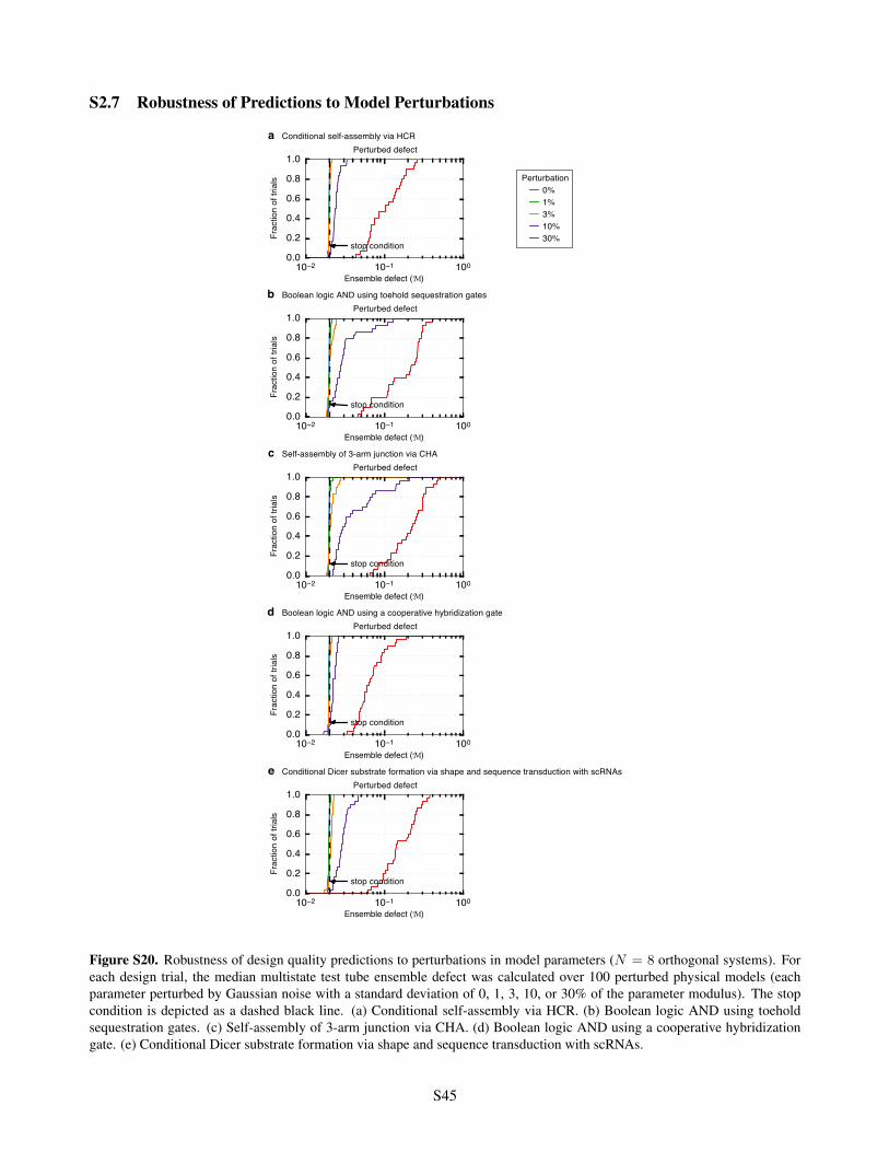
S2.7 Robustness of Predictions to Model Perturbations
10−2 10−1 100
Ensemble defect (M)
0.0
0.2
0.4
0.6
0.8
1.0
Frac
tion
of tr
ials
stop condition
aPerturbed defect
10−2 10−1 100
Ensemble defect (M)
0.0
0.2
0.4
0.6
0.8
1.0
Frac
tion
of tr
ials
stop condition
bPerturbed defect
10−2 10−1 100
Ensemble defect (M)
0.0
0.2
0.4
0.6
0.8
1.0
Frac
tion
of tr
ials
stop condition
cPerturbed defect
10−2 10−1 100
Ensemble defect (M)
0.0
0.2
0.4
0.6
0.8
1.0
Frac
tion
of tr
ials
stop condition
dPerturbed defect
10−2 10−1 100
Ensemble defect (M)
0.0
0.2
0.4
0.6
0.8
1.0
Frac
tion
of tr
ials
stop condition
ePerturbed defect
Conditional self-assembly via HCR
Boolean logic AND using toehold sequestration gates
Self-assembly of 3-arm junction via CHA
Boolean logic AND using a cooperative hybridization gate
Conditional Dicer substrate formation via shape and sequence transduction with scRNAs
Perturbation0%1%3%10%30%
Figure S20. Robustness of design quality predictions to perturbations in model parameters (N = 8 orthogonal systems). Foreach design trial, the median multistate test tube ensemble defect was calculated over 100 perturbed physical models (eachparameter perturbed by Gaussian noise with a standard deviation of 0, 1, 3, 10, or 30% of the parameter modulus). The stopcondition is depicted as a dashed black line. (a) Conditional self-assembly via HCR. (b) Boolean logic AND using toeholdsequestration gates. (c) Self-assembly of 3-arm junction via CHA. (d) Boolean logic AND using a cooperative hybridizationgate. (e) Conditional Dicer substrate formation via shape and sequence transduction with scRNAs.
S45
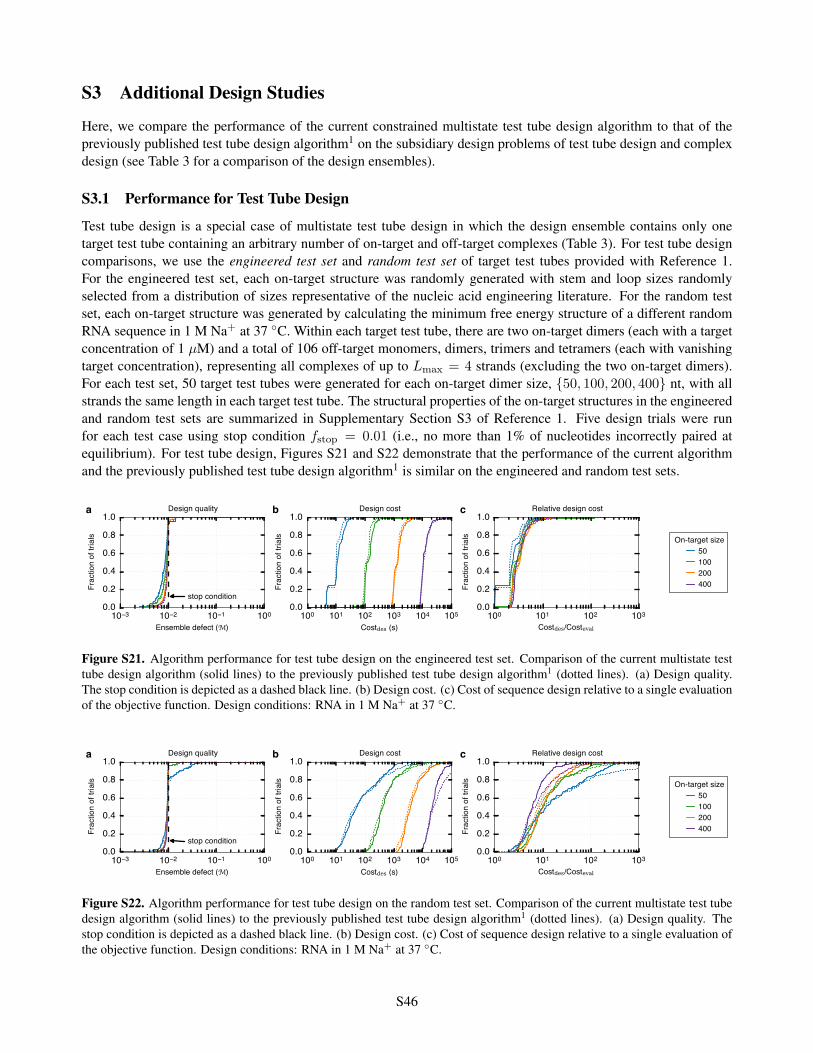
S3 Additional Design Studies
Here, we compare the performance of the current constrained multistate test tube design algorithm to that of thepreviously published test tube design algorithm1 on the subsidiary design problems of test tube design and complexdesign (see Table 3 for a comparison of the design ensembles).
S3.1 Performance for Test Tube Design
Test tube design is a special case of multistate test tube design in which the design ensemble contains only onetarget test tube containing an arbitrary number of on-target and off-target complexes (Table 3). For test tube designcomparisons, we use the engineered test set and random test set of target test tubes provided with Reference 1.For the engineered test set, each on-target structure was randomly generated with stem and loop sizes randomlyselected from a distribution of sizes representative of the nucleic acid engineering literature. For the random testset, each on-target structure was generated by calculating the minimum free energy structure of a different randomRNA sequence in 1 M Na+ at 37 ◦C. Within each target test tube, there are two on-target dimers (each with a targetconcentration of 1 µM) and a total of 106 off-target monomers, dimers, trimers and tetramers (each with vanishingtarget concentration), representing all complexes of up to L
max
= 4 strands (excluding the two on-target dimers).For each test set, 50 target test tubes were generated for each on-target dimer size, {50, 100, 200, 400} nt, with allstrands the same length in each target test tube. The structural properties of the on-target structures in the engineeredand random test sets are summarized in Supplementary Section S3 of Reference 1. Five design trials were runfor each test case using stop condition f
stop
= 0.01 (i.e., no more than 1% of nucleotides incorrectly paired atequilibrium). For test tube design, Figures S21 and S22 demonstrate that the performance of the current algorithmand the previously published test tube design algorithm1 is similar on the engineered and random test sets.
10−3 10−2 10−1 100
Ensemble defect (M)
0.0
0.2
0.4
0.6
0.8
1.0
Frac
tion
of tr
ials
stop condition
a Design quality
100 101 102 103 104 105
Costdes (s)
0.0
0.2
0.4
0.6
0.8
1.0
Frac
tion
of tr
ials
b Design cost
100 101 102 103
Costdes/Costeval
0.0
0.2
0.4
0.6
0.8
1.0
Frac
tion
of tr
ials
c Relative design cost
On-target size50100200400
Figure S21. Algorithm performance for test tube design on the engineered test set. Comparison of the current multistate testtube design algorithm (solid lines) to the previously published test tube design algorithm1 (dotted lines). (a) Design quality.The stop condition is depicted as a dashed black line. (b) Design cost. (c) Cost of sequence design relative to a single evaluationof the objective function. Design conditions: RNA in 1 M Na+ at 37 C.
10−3 10−2 10−1 100
Ensemble defect (M)
0.0
0.2
0.4
0.6
0.8
1.0
Frac
tion
of tr
ials
stop condition
a Design quality
100 101 102 103 104 105
Costdes (s)
0.0
0.2
0.4
0.6
0.8
1.0
Frac
tion
of tr
ials
b Design cost
100 101 102 103
Costdes/Costeval
0.0
0.2
0.4
0.6
0.8
1.0
Frac
tion
of tr
ials
c Relative design cost
On-target size50100200400
Figure S22. Algorithm performance for test tube design on the random test set. Comparison of the current multistate test tubedesign algorithm (solid lines) to the previously published test tube design algorithm1 (dotted lines). (a) Design quality. Thestop condition is depicted as a dashed black line. (b) Design cost. (c) Cost of sequence design relative to a single evaluation ofthe objective function. Design conditions: RNA in 1 M Na+ at 37 C.
S46
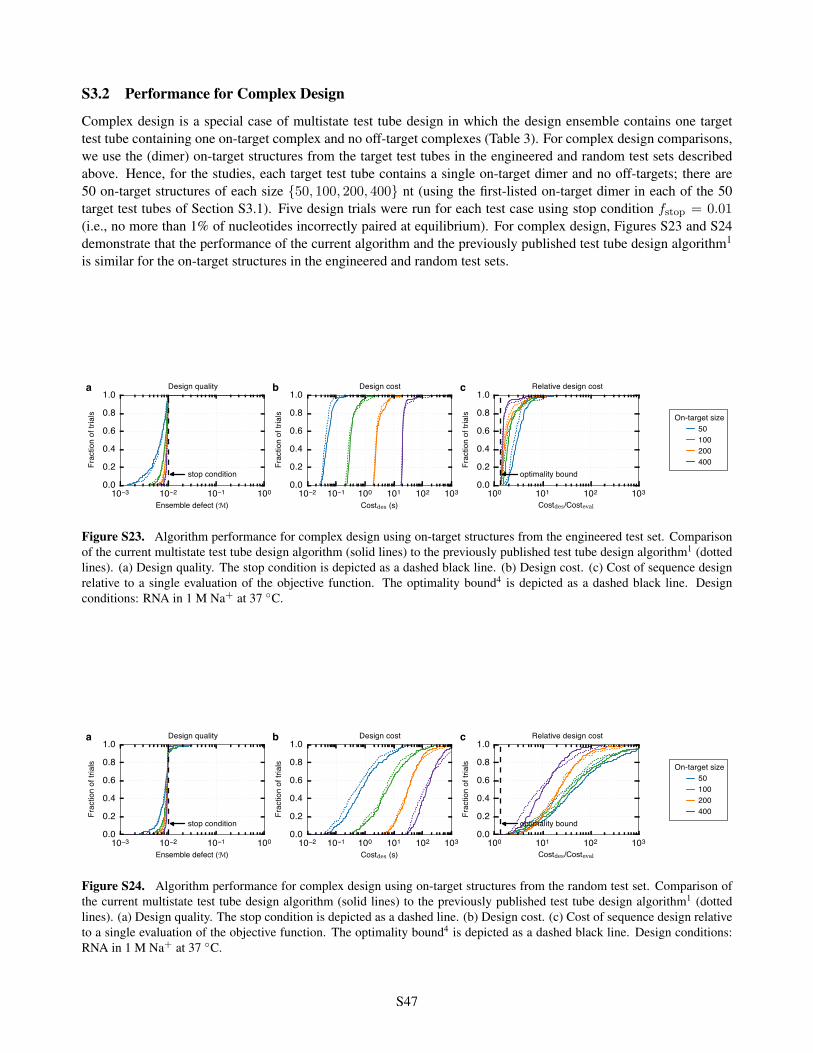
S3.2 Performance for Complex Design
Complex design is a special case of multistate test tube design in which the design ensemble contains one targettest tube containing one on-target complex and no off-target complexes (Table 3). For complex design comparisons,we use the (dimer) on-target structures from the target test tubes in the engineered and random test sets describedabove. Hence, for the studies, each target test tube contains a single on-target dimer and no off-targets; there are50 on-target structures of each size {50, 100, 200, 400} nt (using the first-listed on-target dimer in each of the 50target test tubes of Section S3.1). Five design trials were run for each test case using stop condition f
stop
= 0.01(i.e., no more than 1% of nucleotides incorrectly paired at equilibrium). For complex design, Figures S23 and S24demonstrate that the performance of the current algorithm and the previously published test tube design algorithm1
is similar for the on-target structures in the engineered and random test sets.
10−3 10−2 10−1 100
Ensemble defect (M)
0.0
0.2
0.4
0.6
0.8
1.0
Frac
tion
of tr
ials
stop condition
a Design quality
10−2 10−1 100 101 102 103
Costdes (s)
0.0
0.2
0.4
0.6
0.8
1.0
Frac
tion
of tr
ials
b Design cost
100 101 102 103
Costdes/Costeval
0.0
0.2
0.4
0.6
0.8
1.0
Frac
tion
of tr
ials
optimality bound
c Relative design cost
On-target size50100200400
Figure S23. Algorithm performance for complex design using on-target structures from the engineered test set. Comparisonof the current multistate test tube design algorithm (solid lines) to the previously published test tube design algorithm1 (dottedlines). (a) Design quality. The stop condition is depicted as a dashed black line. (b) Design cost. (c) Cost of sequence designrelative to a single evaluation of the objective function. The optimality bound4 is depicted as a dashed black line. Designconditions: RNA in 1 M Na+ at 37 C.
10−3 10−2 10−1 100
Ensemble defect (M)
0.0
0.2
0.4
0.6
0.8
1.0
Frac
tion
of tr
ials
stop condition
a Design quality
10−2 10−1 100 101 102 103
Costdes (s)
0.0
0.2
0.4
0.6
0.8
1.0
Frac
tion
of tr
ials
b Design cost
100 101 102 103
Costdes/Costeval
0.0
0.2
0.4
0.6
0.8
1.0
Frac
tion
of tr
ials
optimality bound
c Relative design cost
On-target size50100200400
Figure S24. Algorithm performance for complex design using on-target structures from the random test set. Comparison ofthe current multistate test tube design algorithm (solid lines) to the previously published test tube design algorithm1 (dottedlines). (a) Design quality. The stop condition is depicted as a dashed line. (b) Design cost. (c) Cost of sequence design relativeto a single evaluation of the objective function. The optimality bound4 is depicted as a dashed black line. Design conditions:RNA in 1 M Na+ at 37 C.
S47
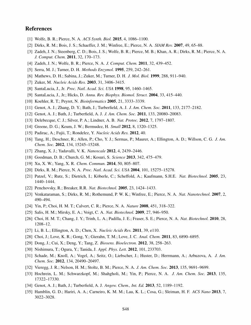
References
[1] Wolfe, B. R.; Pierce, N. A. ACS Synth. Biol. 2015, 4, 1086–1100.[2] Dirks, R. M.; Bois, J. S.; Schaeffer, J. M.; Winfree, E.; Pierce, N. A. SIAM Rev. 2007, 49, 65–88.[3] Zadeh, J. N.; Steenberg, C. D.; Bois, J. S.; Wolfe, B. R.; Pierce, M. B.; Khan, A. R.; Dirks, R. M.; Pierce, N. A.
J. Comput. Chem. 2011, 32, 170–173.[4] Zadeh, J. N.; Wolfe, B. R.; Pierce, N. A. J. Comput. Chem. 2011, 32, 439–452.[5] Serra, M. J.; Turner, D. H. Methods Enzymol. 1995, 259, 242–261.[6] Mathews, D. H.; Sabina, J.; Zuker, M.; Turner, D. H. J. Mol. Biol. 1999, 288, 911–940.[7] Zuker, M. Nucleic Acids Res. 2003, 31, 3406–3415.[8] SantaLucia, J., Jr. Proc. Natl. Acad. Sci. USA 1998, 95, 1460–1465.[9] SantaLucia, J., Jr.; Hicks, D. Annu. Rev. Biophys. Biomol. Struct. 2004, 33, 415–440.
[10] Koehler, R. T.; Peyret, N. Bioinformatics 2005, 21, 3333–3339.[11] Genot, A. J.; Zhang, D. Y.; Bath, J.; Turberfield, A. J. J. Am. Chem. Soc. 2011, 133, 2177–2182.[12] Genot, A. J.; Bath, J.; Turberfield, A. J. J. Am. Chem. Soc. 2011, 133, 20080–20083.[13] Delebecque, C. J.; Silver, P. A.; Lindner, A. B. Nat. Protoc. 2012, 7, 1797–1807.[14] Greene, D. G.; Keum, J. W.; Bermudez, H. Small 2012, 8, 1320–1325.[15] Padirac, A.; Fujii, T.; Rondelez, Y. Nucleic Acids Res. 2012, 40.[16] Tang, H.; Deschner, R.; Allen, P.; Cho, Y. J.; Sermas, P.; Maurer, A.; Ellington, A. D.; Willson, C. G. J. Am.
Chem. Soc. 2012, 134, 15245–15248.[17] Zhang, X. J.; Yadavalli, V. K. Nanoscale 2012, 4, 2439–2446.[18] Goodman, D. B.; Church, G. M.; Kosuri, S. Science 2013, 342, 475–479.[19] Xu, X. W.; Yang, X. R. Chem. Commun. 2014, 50, 805–807.[20] Dirks, R. M.; Pierce, N. A. Proc. Natl. Acad. Sci. USA 2004, 101, 15275–15278.[21] Patzel, V.; Rutz, S.; Dietrich, I.; Koberle, C.; Scheffold, A.; Kaufmann, S.H.E. Nat. Biotechnol. 2005, 23,
1440–1444.[22] Penchovsky, R.; Breaker, R.R. Nat. Biotechnol. 2005, 23, 1424–1433.[23] Venkataraman, S.; Dirks, R. M.; Rothemund, P. W. K.; Winfree, E.; Pierce, N. A. Nat. Nanotechnol. 2007, 2,
490–494.[24] Yin, P.; Choi, H. M. T.; Calvert, C. R.; Pierce, N. A. Nature 2008, 451, 318–322.[25] Salis, H. M.; Mirsky, E. A.; Voigt, C. A. Nat. Biotechnol. 2009, 27, 946–950.[26] Choi, H. M. T.; Chang, J. Y.; Trinh, L. A.; Padilla, J. E.; Fraser, S. E.; Pierce, N. A. Nat. Biotechnol. 2010, 28,
1208–12.[27] Li, B. L.; Ellington, A. D.; Chen, X. Nucleic Acids Res. 2011, 39, e110.[28] Choi, J.; Love, K. R.; Gong, Y.; Gierahn, T. M.; Love, J. C. Anal. Chem. 2011, 83, 6890–6895.[29] Dong, J.; Cui, X.; Deng, Y.; Tang, Z. Biosens. Bioelectron. 2012, 38, 258–263.[30] Nishimura, T.; Ogura, Y.; Tanida, J. Appl. Phys. Lett. 2012, 101, 233703.[31] Schade, M.; Knoll, A.; Vogel, A.; Seitz, O.; Liebscher, J.; Huster, D.; Herrmann, A.; Arbuzova, A. J. Am.
Chem. Soc. 2012, 134, 20490–20497.[32] Vieregg, J. R.; Nelson, H. M.; Stoltz, B. M.; Pierce, N. A. J. Am. Chem. Soc. 2013, 135, 9691–9699.[33] Hochrein, L. M.; Schwarzkopf, M.; Shahgholi, M.; Yin, P.; Pierce, N. A. J. Am. Chem. Soc. 2013, 135,
17322–17330.[34] Genot, A. J.; Bath, J.; Turberfield, A. J. Angew. Chem., Int. Ed. 2013, 52, 1189–1192.[35] Hamblin, G. D.; Hariri, A. A.; Carneiro, K. M. M.; Lau, K. L.; Cosa, G.; Sleiman, H. F. ACS Nano 2013, 7,
3022–3028.
S48
[36] Santini, C. C.; Bath, J.; Tyrrell, A. M.; Turberfield, A. J. Chem. Commun. 2013, 49, 237–239.[37] Choi, H. M. T.; Beck, V. A.; Pierce, N. A. ACS Nano 2014, 8, 4284–4294.[38] Jiang, Y. S.; Bhadra, S.; Li, B. L.; Ellington, A. D. Angew. Chem., Int. Ed. 2014, 53, 1845–1848.[39] Geary, C.; Rothemund, P. W. K.; Andersen, E. S. Science 2014, 345, 799–804.[40] Green, A. A.; Silver, P. A.; Collins, J. J.; Yin, P. Cell 2014, 159, 925–939.[41] Hu, J. M.; Yu, Y. J.; Brooks, J. C.; Godwin, L. A.; Somasundaram, S.; Torabinejad, F.; Kim, J.; Shannon, C.;
Easley, C. J. J. Am. Chem. Soc. 2014, 136, 8467–8474.[42] Machinek, R. R. F.; Ouldridge, T. E.; Haley, N. E. C.; Bath, J.; Turberfield, A. J. Nat. Commun. 2014, 5, 5324.[43] Franco, E.; Giordano, G.; Forsberg, P. O.; Murray, R. M. ACS Synth. Biol. 2014, 3, 589–599.[44] Koos, B.; Cane, G.; Grannas, K.; Lof, L.; Arngarden, L.; Heldin, J.; Clausson, C. M.; Klaesson, A.; Hirvonen,
M. K.; de Oliveira, F. M. S.; Talibov, V. O.; Pham, N. T.; Auer, M.; Danielson, U. H.; Haybaeck, J.; Kamali-Moghaddam, M.; Soderberg, O. Nat. Commun. 2015, 6, 7294.
[45] Zalatan, J. G.; Lee, M. E.; Almeida, R.; Gilbert, L. A.; Whitehead, E. H.; La Russa, M.; Tsai, J. C.; Weissman,J. S.; Dueber, J. E.; Qi, L. S.; Lim, W. A. Cell 2015, 160, 339–350.
[46] Galimidi, R. P.; Klein, J. S.; Politzer, M. S.; Bai, S. Y.; Seaman, M. S.; Nussenzweig, M. C.; West, A. P.;Bjorkman, P. J. Cell 2015, 160, 433–446.
[47] Raschle, T.; Lin, C. X.; Jungmann, R.; Shih, W. M.; Wagner, G. ACS Chem. Biol. 2015, 10, 2448–2454.[48] Takahashi, M. K.; Watters, K. E.; Gasper, P. M.; Abbott, T. R.; Carlson, P. D.; Chen, A. A.; Lucks, J. B. RNA
2016, 22, 920–933.[49] Lee, Y. J.; Hoynes-O’Connor, A.; Leong, M. C.; Moon, T. S. Nucleic Acids Res. 2016, 44, 2462–2473.[50] Zuker, M.; Stiegler, P. Nucleic Acids Res. 1981, 9, 133–147.[51] McCaskill, J.S. Biopolymers 1990, 29, 1105–1119.[52] Hofacker, I.L.; Fontana, W.; Stadler, P.F.; Bonhoeffer, L.S.; Tacker, M.; Schuster, P. Chem. Mon. 1994, 125,
167–188.[53] Lyngsø, R. B.; Zuker, M.; Pedersen, C. N. S. Bioinformatics 1999, 15, 440–445.[54] Dirks, R. M.; Pierce, N. A. J. Comput. Chem. 2004, 25, 1295–1304.[55] Dimitrov, R.A.; Zuker, M. Biophys. J. 2004, 87, 215–226.[56] Andronescu, M.; Zhang, Z.C.; Condon, A. J. Mol. Biol. 2005, 345, 987–1001.[57] Bernhart, S.H.; Tafer, H.; Muckstein, U.; Flamm, C.; Stadler, P.F.; Hofacker, I.L. Algorithms Mol. Biol. 2006,
1.[58] Dechter, R. 2003 Constraint Processing (Morgan Kaufmann, New York).[59] Seelig, G.; Soloveichik, D.; Zhang, D.Y.; Winfree, E. Science 2006, 314, 1585–1588.[60] Zhang, D. Y. J. Am. Chem. Soc. 2011, 133, 1077–1086.[61] McEntyre, J.; Ostell, J. 2002 The NCBI Handbook [Internet] (National Center for Biotechnology Information
(US), Bethesda, MD).
S49