Finance and Economics Discussion SeriesDivisions of Research & Statistics and Monetary Affairs

Federal Reserve Board, Washington, D.C.

Constituencies and Legislation: The Fight over the McFadden Actof 1927

Rodney Ramcharan and Rajan G. Raghuram

2012-61

NOTE: Staff working papers in the Finance and Economics Discussion Series (FEDS) are preliminarymaterials circulated to stimulate discussion and critical comment. The analysis and conclusions set forthare those of the authors and do not indicate concurrence by other members of the research staff or theBoard of Governors. References in publications to the Finance and Economics Discussion Series (other thanacknowledgement) should be cleared with the author(s) to protect the tentative character of these papers.

Constituencies and Legislation: The Fight over the McFadden Act of 19271

Raghuram G. Rajan Rodney Ramcharan Booth School, University of Chicago                 Federal Reserve Board 

Abstract The McFadden Act of 1927 was one of the most hotly contested pieces of legislation in U.S. banking history, and its influence was still felt over half a century later. The act was intended to force states to accord the same branching rights to national banks as they accorded to state banks. By uniting the interests of large state and national banks, it also had the potential to expand the number of states that allowed branching. Congressional votes for the act therefore could reflect the strength of various interests in the district for expanded banking competition. We find congressmen in districts in which landholdings were concentrated (suggesting a landed elite), and where the cost of bank credit was high and its availability limited (suggesting limited banking competition and high potential rents), were significantly more likely to oppose the act. The evidence suggests that while the law and the overall regulatory structure can shape the financial system far into the future, they themselves are likely to be shaped by well organized elites, even in countries with benign political institutions.

1 Raghuram Rajan: rajan@chicagobooth.edu, Rodney Ramcharan: Rodney.Ramcharan@frb.gov. We thank Edward Scott Adler, Daron Acemoglu, Lee Alston, Charles Calomiris, Price Fishback, Oded Galor, Sebnem Kalemli-Ozcan, Gary Richardson, Howard Rosenthal, Eugene White and seminar participants at the IMF, and the NBER Development of the American Economy and Income Distribution and Macroeconomic Groups for useful comments. Rajan thanks the Stigler Center for the Study of the State and the Economy and the Initiative on Global Markets, both at the University of Chicago’s Booth School, as well as the National Science Foundation, for funding. Keith T. Poole and Kris James Mitchener kindly provided data.

2

Constituencies or interest groups that arise from the pattern of land holdings or

other forms of economic production in a country can shape important economic

institutions such as the financial system, and consequently, economic development

(Engerman and Sokoloff (2002, 2003), Haber (2005), Rajan and Ramcharan (2011)). But

the channel through which interest groups might operate remains a matter of debate.

Some (see, for example, Acemoglu, Johnson, and Robinson (2005)) argue that the

mediating channel is political institutions, as elite interest groups create coercive political

institutions that give them the power to hold back the development of economic

institutions, such as finance, and hence economic growth. However, legislation, and its

effects on perpetuating rents and hence political power, may be another principal channel

through which constituencies might shape the financial system and project their influence

through time, even in benign democratic political systems (see Do (2004), Glaeser,

Scheinkman, and Shleifer (2004), or Mian et. al (2010), for example).

In this paper, we study whether, and how, constituencies influence the

development of the financial system, using evidence from congressional voting on the

McFadden Act of 1927. The United States has long had a dual banking system, where

state banks are chartered and regulated at the state level, while national banks operate

under federal oversight. Before the McFadden Act, some states allowed state banks to

open multiple branches, while others prohibited all branching. However, nationally

chartered banks were, in all cases, not allowed to open branches (Cartinhour and

Westerfield (1980), Southworth (1928)). As a result, an increasing number of national

banks gave up their charter (which typically meant their leaving the Federal Reserve

3

System also).2 The McFadden Act attempted to level the playing field by forcing states to

accord largely the same branching rights to national banks as to state banks (Preston

(1927)). It was the key piece of federal legislation regulating bank branching, and hence

bank competition, in the United States for about 70 years—up until the passage of the

Riegle-Neal Act in 1994.

The act proved enormously controversial, and a study of how the vote of each

congressional district varied with the constituencies in that district can be extremely

informative on (1) whether constituencies had political influence; and (2) whether the

influence was directed in expected ways for, or against, greater competition and financial

development. Of course, there has already been an enormous amount of work on the

political economy of the McFadden Act (see, for example, Economides, Hubbard, and

Palia (1996)). Much of the work has examined whether legislators from states with unit

banks voted disproportionately against the Act, and the results are mixed at best – for

instance, Economides, Hubbard, and Palia (1996) find that the influence of the proportion

of banks with branches in the state on the fraction of state representatives voting for

branching is negative and insignificant (though they find that states with poorly

capitalized state banks voted against branching). Our contribution is to dive deeper into

the determinants of the constituencies against branching within state. This allows us to

focus on a richer, and more detailed, pattern of interests than previously examined, as

2 The Comptroller of Currency in 1922 observed: “National banks are compelled to compete with state institutions. If state laws are more liberal they will constitute an inducement to banks to operate under the laws of the states rather than the Nation…If the system is to be perpetuated there must be national banks in sufficient number and strength…they must be given charters liberal enough to remain in the system. The advantage of the more liberal conditions that can be enjoyed outside the national banking system…will presently become a menace to the strength, and may ultimately threaten the very existence, of the Federal Reserve System (Report of the Comptroller of Currency (1922)).

4

well as exploit within state differences in voting patterns. Unlike previous work, we find

strong evidence of constituency influence.

In Rajan and Ramcharan (2011), constituencies do appear to influence the

structure of the financial sector. Specifically, landed elites—a key political constituency

during this period--were successful in restricting local bank competition in different

counties in the United States. Counties where the agricultural elite had disproportionately

large land holdings had significantly fewer banks per capita, even correcting for state

level effects. Moreover, credit appears to have been costlier, and access to it more

limited, in these counties.

The literature suggests three main reasons why landed interests might have

opposed more local bank competition. First, limits on bank competition and control over

exit could provide landowners insurance during periods of agricultural distress. While

large national banks or state banks with branches could foreclose more easily on loans

and exit the locality, transferring capital to urban or less distressed rural areas, small local

banks would have fewer options, and would have to continue lending to large local

farmers during periods of distress (Calomiris and Ramirez (2004)).

Second, control over bank entry could accord landed interests greater influence

over the local financial system, enabling them to prevent or delay the emergence of

alternative centers of economic power and status (Chapman (1934)). For example, a

rapidly growing manufacturing sector could increase the returns to schooling and attract

labor away from agriculture, and there is evidence that landed interests may have used

5

their political influence to restrict not just finance, but education and other public goods

(Galor et. al (2009), Ramcharan (2010)). 3

Third, large landowners generated surpluses which they could lend. They also

often had a stake in, or influence over, the local bank. The entry of more formal credit

institutions could be competition for their lending business. They also had indirect

reasons to keep out competition in lending. Landowners often owned the local store.

Tenants and small farmers needed credit to buy supplies from the local store. By limiting

credit from alternative sources – for instance by keeping banks out -- the local merchant

cum landlord could lock the farmer in and charge exorbitant prices, perpetuating the

lucrative debt peonage system (Haney (1914, p55-56).4 5 There is, however, some

controversy among economic historians about the extent of debt peonage and the

“bankability” of tenant farmers and share croppers during this period.6

3 Alston and Ferrie (1993) argue that because landed interests wanted to maintain a paternalistic state in order to ensure a steady supply of farm labor, the Southern congressional delegation systematically blocked the development of the federal welfare state in the U.S. until mechanization reduced the demand for unskilled labor.

4 Initially, there was a conflict of interest between large landlords and the local merchant because both had an interest in tenant farmers. But “as time went on the two classes tended more and more to become one.” Landlords were drawn into the store business by “the desirability of supplying their tenants ”, while “storekeepers frequently became landowners by taking over the farms of those who were indebted to them or by direct purchase at the prevailing low price”. Hicks (1931, p32). Haney (1914, p54) writes that in most parts of central Texas, “over 90 percent of those tenants who owe the store are also indebted to their landlords for larger or smaller advances.” See also the surveys in Goodwyn (1978) and Ransom and Sutch (2001).

5 There were other benefits for the rich landlord to limiting access. Landlords would also enjoy a competitive advantage, for instance by being able to buy land cheaply when small farmers were hit by adversity, or by having privileged access to loans in the midst of a prolonged drought.

6 For example, the evidence in Fishback (1989) suggests that most farmers may have been able to repay their debts shortly after harvests. Also, while debt peonage is most closely associated with racial discrimination, Alston and Kauffman (2001) find little evidence of discrimination in sharecropper pay for a sample of southern counties. However, the most extreme versions of debt peonage (forced land sales because of distress, racial discrimination, etc.) need not apply for landowners cum storeowners to have an incentive to monopolize credit.

6

While we know the landed elite had the incentive and the ability to influence

outcomes, we do not know whether their influence worked through the political process.

For instance, Rajan and Ramcharan (2011) argue that landed elites could have shaped

local bank competition by giving business to favored banks. Indeed, if politicians were

strictly motivated by doing good for the mass of voters (the public interest view of

legislation), it seems unlikely that they would have sided with the views of the landed

interests. If, however, concentrated money power trumped dispersed voter interests, one

might expect a district’s politicians to reflect the interests of the landed elite (the private

interest view).7 If so, we should see representatives of districts where landed elites were

important vote disproportionately against the McFadden Act.

The McFadden Act proposed to extend bank branching powers to national banks

only in those states that already allowed state banks the right to open branches.

Contemporary texts (see, for example, Preston (1927)) suggest that the expectation was

that if the McFadden Act allowed national banks liberal branching powers, then

subsequent to the passage of the act, national banks would unite with large state banks to

push for branching in all states. Thus landed elites in non-branching states could be

expected to be even more opposed to the McFadden Act than were landed elites in

branching states, especially because the latter’s rents would already have been diminished

by branching by state banks.

7 There is evidence that local politicians had some influence over bank structure, over and above their votes on legislation. For example, members of Congress often influenced bank chartering decisions in their district. Referring to state charter applications, American Bankers Association (1935) quotes a Comptroller on political influence: “prior to the disposition of an application a copy thereof is sent to the national-bank examiner, to the Member of Congress for the district in which the bank is located, and to the superintendent of the state banking department, with request for information on the character and standing of the applicants, the existing demand for a bank at the locality, and an expression of opinion as to whether success is probable.”

7

The Act evolved in Congress as constituencies worked to influence the

legislation. Examining the initial congressional roll call data, controlling for state fixed

effects (which allow us to absorb state differences in regulations, among other factors),

we find that congressmen from districts with more concentrated land holdings (our proxy

for the relative importance of landed interests) were far more likely to oppose the

McFadden Act during its first House vote in 1926. The results are stronger still when we

instrument land concentration with a technological determinant of the optimal size of

land holdings, the pattern of rainfall in the area.

The association of land concentration with congressional opposition was

especially strong in those districts where agriculture was relatively more important than

manufacturing, suggesting that landed elites were politically more effective when they

also dominated economically. Similarly, the association of landed interests with

congressional opposition was particularly strong in non-branching states, perhaps because

of the fears of the local elite about the incipient spread of branching.

Also, using hand collected data from the 1930 Census on measures of credit cost

and access, such as the interest rate and loan to value ratios of farms, we find that

congressional support for the McFadden Act, was significantly lower in those districts

with high credit costs and limited credit availability, suggesting that the desire to protect

incumbents’ rents may have indeed inspired political opposition to the Act.

We use the legislative history of the McFadden Act to help identify more

precisely the role of landed interests in shaping its passage. Some of the more aggrieved

landowners, especially those in smaller communities, were appeased by provisions that

were introduced into the act limiting the ability of national banks to open branches in

8

small towns. The historical commentary also suggests that political horse-trading in the

House may have been key in securing the Act’s final passage, as government price

support for grain was extended to cotton and tobacco, allegedly in order to entice the

Southern delegation to support the McFadden Bill and break the deadlock with the Senate

(the House disagreed with the Senate version that was more favorable towards bank

competition). Consistent with this narrative, we find evidence that the association

between congressional opposition and the strength of landed elites declined significantly

in tobacco growing districts, ensuring the Act’s passage.

Finally, using county level data, we explore the impact of the Act on local

banking structures. There is evidence that in those states allowing branching, the Act’s

passage did lead to faster national bank growth, and a decline in deposits held in state

banks. The legislation thus had a significant impact on local bank structures.

Eventually, technological changes in banking, which allowed banking at a

distance, made it hard to maintain bank branching restrictions in the US (Kroszner and

Strahan (1999)). The Riegle-Neal Act repealed the remaining restrictions on bank

branching in 1994. A summary evaluation then is that by restricting the scope of the

McFadden Act and protecting small banks from competition, landed interests

strengthened small community banks, which gained political influence and maintained

the protections long after their initial protectors lost their economic and political heft.

Thus constituencies can have influence long after they pass from the scene.

Ours is not the first paper to show that landed interests matter for financial

development (see, for example, Rajan and Ramcharan (2011), and Vollrath (2009)).

While Rajan and Ramcharan (2011) argue that landed interests have influence that helps

9

them restrict local bank entry and competition, they do not provide evidence of such

influence working through political channels and congressional votes. The pattern of

voting on the McFadden Act helps us establish the necessary link between landed

interests and political influence.

Finally, there is an extensive literature on the political economy of banking

legislation more generally (for recent examples, see Acharya, van Nieuwerburgh,

Richardson and White (2011), Brown and Dinc (2005), Dinc (2005), Cetorelli and

Strahan (2006), Mian, Sufi, and Trebbi (2010), or Igan, Mishra, and Tressel (2011)). Our

incremental contribution to the widely accepted finding that narrow directly-affected

interest groups influence legislation is to demonstrate the influence of deeper (possibly

technologically-determined) constituencies that drove one of the most salient pieces of

financial legislation in U.S. history.

In the next section we briefly describe the Act. We describe the data in section III,

the main results are in section IV, we discuss the impact of the act on bank structures in

section V, and then conclude.

I. THE MCFADDEN ACT

The Federal Reserve Act of 1913 did not grant national banks branching rights.

National bank regulators therefore feared that the national banks would not be

competitive with state banks in states that allowed state banks branching powers. The

Comptroller of the Currency ruled in 1922 that national banks could open intra-city

offices for the purpose of collecting deposits when this did not conflict with state laws

(see White (1985)). Two days after the Comptroller’s ruling, the First National Bank of

St. Louis opened a full-fledged branch and argued that, as a federally chartered

10

institution, it was not subject to state regulation. Two years later, the Supreme Court

ruled against it, but the fight had been joined.

Fearing that once the national banks got branching powers, they would join large

state banks in pressing for branch banking in every state, banks in many of the unit

banking states formed state associations that declared themselves opposed to branch

banking. On the national level, the United States Bankers Association Opposed to Branch

Banking was formed. Unit bankers pressed their state legislatures to remove any

ambiguity about whether branching banking was prohibited, and by 1924, nine states

added anti-branching provisions to their banking laws.

The McFadden Act was motivated by the federal government’s desire to resolve

the ambiguity about the powers of national banks, and preserve the attractiveness of

national bank charters and membership in the nascent Federal Reserve System against

regulatory competition from state bank regulators. It provided that in states where state

branch banking existed, or could exist in the future, both national and state bank members

of the Federal Reserve System would be allowed to operate branches within the city

limits of the parent bank. This was viewed as a step towards further branching

liberalization and greater bank competition at the local level.

The local political constituencies who had historically guarded their control of the

banking system saw their rents threatened by the prospect of increased competition and

the potential dominance of local banking by large national banks. Moreover, as discussed

above, they feared that the Act would lead to more states opening up to branching.

Opposition to branching was also intense in those areas with many small unit banks. The

1920s was a period of agricultural distress, and rural small bank failures became

11

increasingly common. These unit bankers feared that the introduction of bank branching

and the entry of large national banks into small towns could accelerate small bank

failures. The Mid West, especially Chicago, heavily populated with small unit banks,

became the epicenter of opposition to the McFadden Act (see Chapman and Westerfield

(1980), Southworth (1928), White (1985)).

As an aside, we should note that while the landed elite may have been concerned

by the pro-competitive aspects of the McFadden Act, Populist forces may have pushed

for preserving unit banking because it limited the power of distant bankers. Politics

makes strange bedfellows -- different constituencies may make common cause over

regulations because they like different aspects of it, even though the constituencies

fundamentally oppose each other. Moreover, popular populist policies – keep banking

local – may capture the public’s imagination even if they are not broadly good for the

populace, or framed with their interests in mind. Our detailed examination of district-by-

district voting patterns can help us focus on local influences, which may be lost if we

were to examine state-level voting patterns, as some previous studies have done.

The Act went through several metamorphoses in Congress, as the various

constituencies sought to influence the legislation. In its original form, before February of

1926, the branching issue was phrased in language widely viewed as favoring further

branching and local competition. 8 But the Hull amendment, which delayed the Act’s

passage amid much controversy, sought to “limit bank branching to those States which

permitted branch banking at the time of the approval of the bill—so far as the national

8 Specifically, this version of the Act “provided that state bank members of the Federal Reserve System might not establish branches outside their home cities and that national banks might establish branches in their home cities in those states where state banks were accorded a like privilege ”Collins, “Report on the Bank Branching Question”, pp 82-83.

12

banking and the Federal Reserve Systems are concerned.” In so doing, the amendment

was intended to preserve the coalition against the spread of branching, thus allowing the

act to obtain support from unit-banking states. That is, the Hull amendment would ensure

that any subsequent legislation to permit branching would encounter three-fold

opposition from (1) national banks that could not now have branches in those states (2)

the state bank members of the Federal Reserve System, who also could not have any

branches in those states (3) and of course, the incumbent unit bankers. The Hull

amendment was dropped from the final bill before it passed.

In sum, the sections pertaining to branching in the Act were vigorously contested,

right from the Act’s introduction in the House in 1922 through its final passage in 1927,

which was assured only after the Senate invoked a cloture motion for the third time in its

history at that point. The Act was signed into law by President Coolidge in February

1927.

Clearly, unit banks were opposed to the Act. But what interests lay behind the unit

banks? As we argue in the introduction and in Rajan and Ramcharan (2011), landed

agrarian interests were strongly opposed to any reforms perceived to be fostering more

local bank competition. In what follows, we will attempt to tease out the role of these

deeper interests in opposing competition.

II. DATA

A. LAND CONCENTRATION

What could be a proxy for the strength of landed interests and their desire to limit

access to finance? In any of these hypotheses where there is a group of larger farmers

who “exploit”, there has to be another group of small farmers or tenants who are

13

explicitly “exploited” (as in the debt peonage hypothesis) or are implicitly “exploited”

(for instance, if they contribute savings to the local pool but do not get loans in a

downturn because their access to finance is deliberately left underdeveloped, as in

Calomiris and Ramirez (2004)). One measure of the strength of these two constituencies

is the Gini coefficient of land farmed, which measures the degree of inequality of land

holdings. If land holdings are very unequal, large landowners could have both the ability

and incentive to limit access to finance, while if land holdings are relatively equal

(whether uniformly large or small), no one has the power or the interest to alter access for

others.9

Our measure of the concentration of land holdings is based on the distribution of

farm sizes as in Rajan and Ramcharan (2011). The data are collected by the U.S. Census

Bureau at the county level for 1920. A farm is defined as “all the land which is farmed by

one person, either by his own labor alone or with the assistance of members of his

household or hired hands”. Note that a tenant is also a farmer by this definition. We have

information on the number of farms falling within particular acreage categories or bins,

ranging from below 3 acres up to 1000 acres. Assuming the midpoint of each bin is the

average size of farms in that bin, we construct the Gini coefficient to summarize the farm

acreage data (see Appendix for a precise formula and definitions). The Gini coefficient is

a measure of concentration that lies between 0 and 1, and higher values indicate that

farms at both ends of the size distribution account for a greater proportion of total

agricultural land—that is, the holding of agricultural land is unequally distributed.

9 This presupposes, of course, that those without land either do not have the basic minimum surplus to be worth squeezing (such as field hands) or live in towns, far from the sphere of influence of the landlords. We will show that a greater fraction of activity in manufacturing (a measure of non-land activity) does diminish the effect of land concentration on opposition to the Act.

14

In 1920, the average Gini coefficient of a county is 0.426, the 99th percentile

county is at 0.687, the 1st percentile county is at 0.2, and the standard deviation is 0.10.

The correlation between the Gini for a county and the share of agricultural land in small

farms (below 20 acres) is positive, as is the correlation with the share in large farms

(above 175 acres). The correlation between the Gini and the share in medium sized farms

(between 20 acres and 175 acres) is negative. Thus counties with high Gini coefficients

tend, as we would expect, to have more land in both small, as well as large, farms.

Interestingly, as a result of the greater weight in small farms, counties with Gini above

median have smaller farms on average than counties with Gini below median.

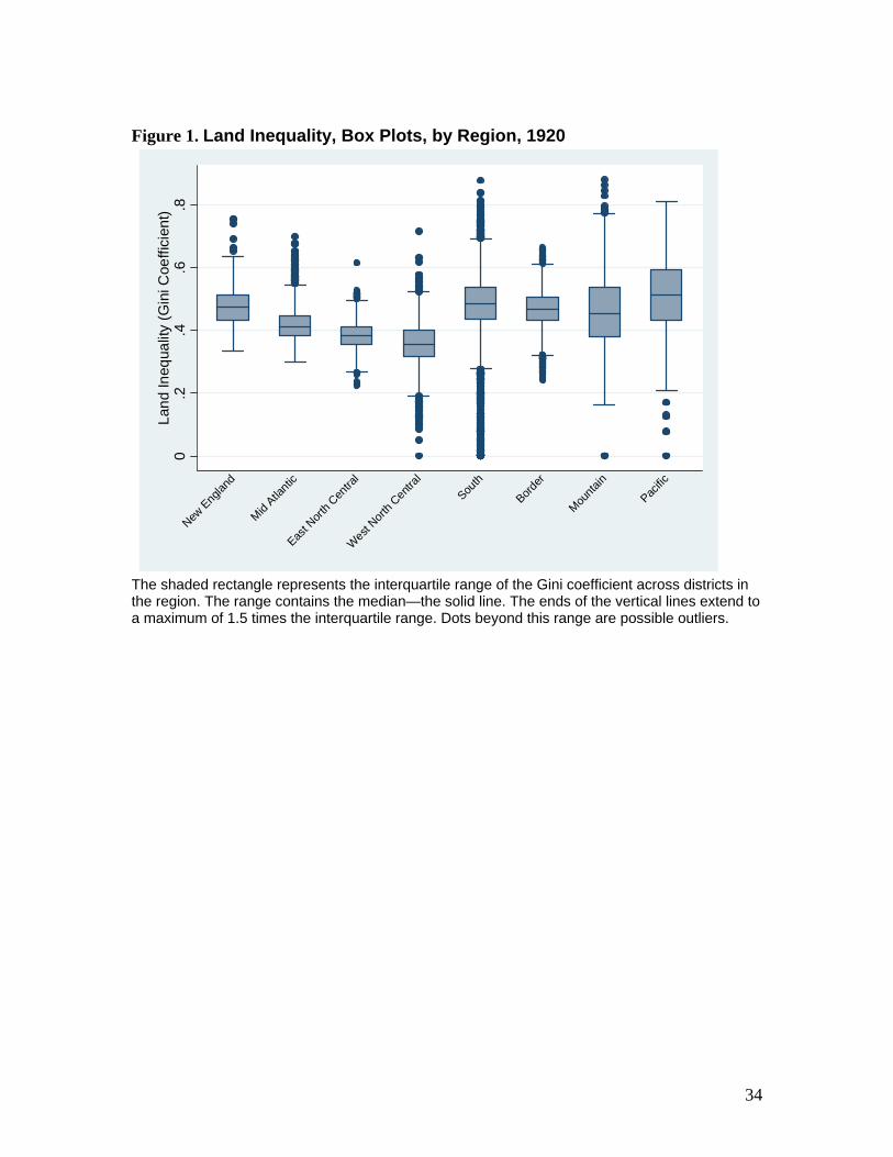
This pattern of correlations between the Gini coefficient and farm sizes suggest

that agricultural production might have been increasingly dominated by a landed elite in

those counties with a higher Gini coefficient. Figure 1 indicates that the Southern and

Border counties, areas known for plantation agriculture, generally had higher Gini

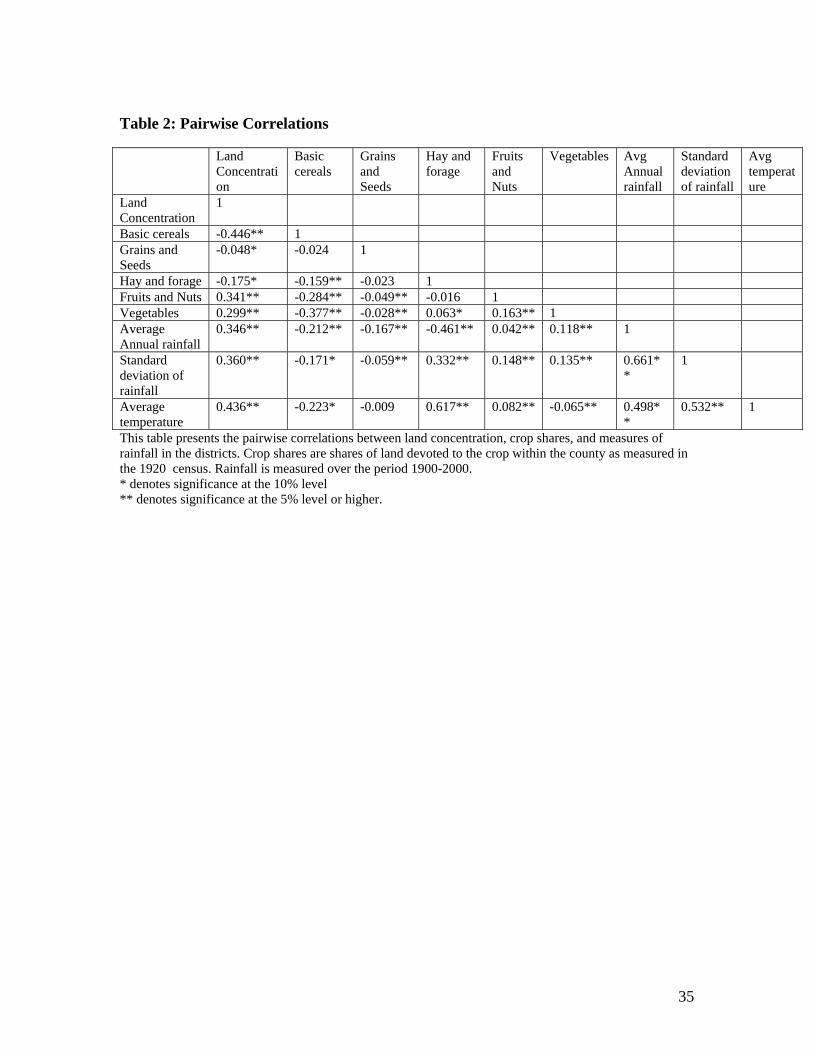
coefficients than elsewhere. Similarly, the correlations in Table 2 suggest that areas with

high levels of land concentration tended to have higher levels of rainfall, a key

requirement for plantation crops like cotton and sugar; counties with higher Gini

coefficients also tended to specialize less in grain and other crops more suited to

independent smaller family farms, given the technologies of the era (see Ramcharan

(2010) and the references contained therein). All this also suggests that land

concentration was determined substantially by technological forces outside finance.

B. Congressional District Votes

The McFadden Act was first introduced into the 69th Congress on Feb 4th, 1926.

There is a weak positive correlation between the percent of a state’s congressional

15

delegation that voted against the Act and the average level of land concentration within

that state in 1920. But the voting behavior of House members, in contrast to the Senate, is

designed to reflect the interests of local constituents rather than aggregate state level

issues, and we focus more systematically on the district level voting data (see Rusk

(2001) and references contained therein).

To this end, we merge the detailed county level data on land concentration and

other demographic, geographic, and economic variables with the congressional district

voting data on the McFadden Act. There are about 3000 counties surveyed in 1920

Census, but only 427 districts in the 69th Congress, which were apportioned based on the

population estimates from the 1920 Census. In about 330 cases there is a direct

correspondence between congressional districts and counties: one or more whole counties

are aggregated into a single district. In these cases, we construct the district level data by

aggregating the “whole” county level data using basic measures of central tendency such

as the mean and weighted by each county’s relative size in the district. For instance, the

First congressional district of Maine is comprised of both Cumberland and York counties,

and we use the population weighting scheme: each county’s characteristic is attributed to

the First district in proportion to the county’s relative population in the district.

However, for about 20 districts, counties have either been split into several

districts, or pieces of various counties and towns have been combined to form a district.

We call these cases “splits” and they primarily occur in urban areas. For example,

Manhattan (New York county ) was “split” or divided into 11 different districts in the

69th Congress. For county level data in the “split” districts, we simply ascribe the

county’s characteristics uniformly to those districts contained within the county (Adler

16

(2002)). Some districts were however formed from towns and were omitted from the

sample as there is no correspondence with county level data. We are thus left with a

sample of 354 congressional districts.

In Table 3A, we decompose the initial vote on Feb 4th, 1926, and this suggests

that the voting pattern in the available sample of districts is similar to the full roll call

data – 66 percent voted Yea and 23 percent voted Nay in the available sample versus 67

percent and 21 percent respectively in the full roll call vote. And while 80 percent of

House Republicans and only 47 percent of the Democrats voted in favor of the act, this

difference in support across party lines largely reflected varying regional economic

interests rather than ideological differences (Southworth (1928)). For instance, from

Table 3B we see that opposition was mainly concentrated in the agrarian South, and parts

of the upper mid West.

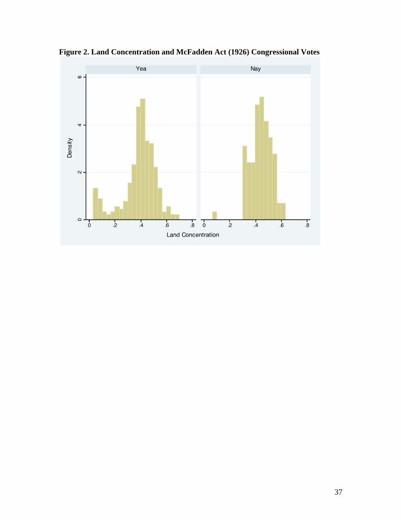
The correlation between land concentration and a “Nay” vote is 0.17, which is

significant at the 5 percent level. Also, Figure 2, which plots the distribution of land

concentration by ”Yea” and “Nay” votes, suggests that House members from districts

with a greater similarity in the size of land holdings—“more equal counties”—were far

more likely to vote in favor of the legislation than those from more unequal districts.

These differences across the two distributions are significant at the one percent level. Of

course, this non parametric evidence is only suggestive; omitted demographic,

geographic, and economic variables might explain the motivation for opposition to the

Act, rather than simply the influence of landed interests. We thus use the legislative

history of the Act to understand the role of landed interests in shaping the legislation.

17

III. RESULTS: LAND CONCENTRATION AND THE MCFADDEN ACT

A. THE INITIAL BILL, 1926

To this end, in the first two columns in Table 4A we use a simple linear

probability model to measure the relationship between land concentration within a

congressional district and the probability that the district’s representative voted against

the McFadden Act in its initial form on February 4th 1926. Specifically, omitting the

abstentions and paired votes, the dependent variable equals 1 if a congressman voted

against the act, and 0 if he voted “Yea”. We also include state-level indicator variables in

all specifications to control for the potential impact of state level factors on the House

vote. These correct for state level differences in regulations such as unit versus branch

banking and presence of deposit insurance, as well as other differences such as average

capital levels (Economides, Hubbard, and Palia (1996)) that the prior literature has

focused on.10

Consistent with the non-parametric evidence, there is a statistically significant and

large positive relationship between the probability of a “Nay” vote and land concentration

in column 1. A one standard deviation increase in land concentration is associated with a

0.05 increase in the probability of observing a “Nay” vote; recall that the unconditional

probability of a “Nay” vote in the sample is 0.26.

There are, of course, important district-level differences we should correct for.

We include a broad array of geographic and demographic controls in Table 4A column 2.

10 The bicameral nature of the Congress and the design of House terms are intended to make House members more responsive to local interests than the Senate, but aggregate state and regional factors might still affect House voting patterns. For example, state level “machine” politics might sway the House delegation from a given state to vote in a particular way. Likewise, broad regional interests—the Mid West and South were far more agrarian than other parts of the country—could also sway the voting behavior of a state’s House delegation (Rusk (2001)).

18

Waterways were centers of economic activity as well as transportation (and if freshwater,

of irrigation). For instance, waterways such as the Great Lakes in the upper mid west, and

the Atlantic Ocean along the East coast helped spur industrialization and the demand for

financial services in those regions (Pred (1966)). And including these variables help

control for plausibly exogenous determinants of a district’s prosperity and the kind of

economic activity it might undertake. The socioeconomic controls include: the fraction of

the district’s population that is illiterate, the fraction that is young, and the fraction that is

black. Also included are the log of district population, as well as the fraction of the

population that is urban (reflecting the fact that urban interests vis a viz banking might

have differed from rural groups).

In addition, we also include as controls the ideology index developed by Poole

and Rosenthal (2007) for each congressman voting on the Act. The first dimension of the

index is generally interpreted as the congressman’s preference for redistribution—liberal

or conservative bias. The second dimension focuses on urban relative to agrarian biases.

Since both dimensions probably influenced voting on the act, we include both indices,

recognizing that we may be overcorrecting since the landed elite might well determine

the ideological preferences of the congressman in power. In this, our baseline

specification, the coefficient estimate on land concentration in Table 4 column 2 nearly

doubles, and remains significant at the 5 percent level.

The concentration of land holdings might be related to the value of land

ownership itself, and there is some evidence that the value of landownership may have

directly affected preferences for different types of bank structures. For example,

Calomiris and Ramirez (2004) find evidence that unit banking was more likely in states

19

with higher farm wealth, suggesting that the returns to preserving local bank lending

might have been higher in those states where land was more valuable. In column 3, we

control for the per capita farm wealth within the congressional district—the value of land,

crops, buildings and implements divided by the farm population. The coefficient estimate

on land concentration increases slightly in magnitude, suggesting it is not a proxy for per-

capita farm wealth. Interestingly, per capital farm wealth, while positive, is not

statistically significant. Also, because the land concentration measure does not

distinguish between forms of ownership, in results available upon request, we control for

the share of tenant farmers within the congressional district. This variable is not

significant (p-value=0.63), while the land concentration coefficient is largely unchanged

relative to column 2.

Land concentration may not be exogenous to banking structure. For instance,

areas with small, and relatively few, banks may have relatively concentrated banking

markets, which in turn may result in land concentration. Put differently, our discussion

above has been based on an assumption that land concentration is the deeper driving

variable. To address concerns about this assumption (and to place identification on firmer

ground), we exploit the variation in land concentration that can arise from the plausibly

exogenous variation in rainfall.

Rainfall patterns can shape the pattern of agricultural production. Plantation

crops, such as cotton and sugar, are better suited to areas with plentiful rainfall, while

wheat and grain, which were often grown on smaller more uniform plot sizes during this

period, thrive in areas with less precipitation (Gardner (2002), Tomich, Kilby and

Johnston (1995) and the references in Rajan and Ramcharan (2011)). Consistent with

20

these ideas, there is a large first stage conditional correlation between land concentration

and the log average rainfall in the district—reported in the notes to Table 4A.

In column 4, we use average rainfall as an instrument for land concentration. The

IV results are less precisely estimated (p-value=0.09), but the coefficient is about 80

percent larger than the OLS estimate in column 2. As a robustness check, in column 5,

we include both the average rainfall, as well as its standard deviation jointly as

instruments. The latter is a common measure of weather risk, and has also been shown to

affect the pattern of land holdings in the United States during this period (Ramcharan

(2010)). As described in the notes to Table 4A, both variables are individually and jointly

positively associated with land concentration. The estimates for instrumented land

concentration in columns 4 and 5 are similar, and the over-identification test that the

availability of two instruments permits us lends some plausibility to the exclusion

restriction assumption, suggesting that land concentration in the district may have played

an economically important role in shaping voting outcomes.

While the results using the rainfall instrument are reassuring about the direction of

causality, congressional districts club together areas with varied rainfall patterns. This

introduces noise, which is especially problematic when we split the sample, as some

robustness tests require. Therefore, in the robustness exercises that follow, we will revert

to the more conservative OLS estimates, though IV estimates are available on request.

In Table 4B, we perturb the baseline specification in a number of different ways

in order to better understand the role of landed interests on voting outcomes. The relative

economic clout of agrarian interests within a district might affect their ability to influence

the political process. During this period the manufacturing sector, an important consumer

21

of financial services, was growing, and becoming increasingly politically powerful. And

in those districts where the economic power of the agricultural sector was offset by the

power of the manufacturing sector, the influence of land concentration on congressional

voting behavior might have been more muted. Conversely, in districts in which landed

interests were the dominant economic power, they would likely wield greater political

power, and thus, have greater influence over congressional district voting behavior.

We thus exploit the variation in the underlying economic structure across districts

in order to understand better the possible role of landed interests and other constituencies

in shaping the legislation. One measure of the relative economic power of the

manufacturing sector is the ratio of the value of manufacturing output to the value of

manufacturing and agriculture output in 1920. In Table 4B Column 1, we include the

interaction between manufacturing share and land concentration in our baseline

regression, taking care to include manufacturing share and its square directly. The

estimates suggest that the positive impact of land concentration on congressional

opposition to the Act was significantly more muted in those districts in which

manufacturing was economically more important. For a district at the 25 percentile share

of manufacturing in output, a one standard deviation increases in land concentration is

associated with a 0.18 increase in the probability of observing a “Nay” vote. However,

for a district at the 75 percentile, with a relatively economically important manufacturing

base, a similar change in land concentration suggests only a 0.12 increase in the

probability of a “No”.11

11 Clearly, we cannot rule out the possibility that the extent of manufacturing share (or of national bank share, see below) was endogenous – areas where agrarian interests were stronger held back financial development and hence industrialization. This is not inconsistent with our point that the extent of

22

National banks obviously stood to gain from the Act’s passage, possibly at the

expense of small state unit banks, and we next explore the association between the

existing structure of the local banking system and local political support for the act. In

Table 4 Column 2, we include the share of national banks in total banks within the

district in 1920 (and thus unaffected by the Act’s passage in 1927). The coefficient

estimate indicates that congressional opposition to the Act was significantly attenuated in

those districts in which national banks were more dominant in the local banking system.

A one standard deviation increase in this share suggests a 0.05 decline in the probability

of observing a “Nay” vote.

Clearly, districts with few banks or with smaller banks may have been

differentially disposed to vote on the legislation. To proxy for the relative number of such

banks, we include the per capita number of state banks, and to proxy for bank size, we

include the average value of deposits in each state bank in the district in Table 4B

Column 3. Of course, these “explanatory” variables are endogenous since we have argued

that bank structure is shaped by landed interests, and we must be careful in drawing

strong conclusions from this exercise. Nevertheless, it is interesting that in Table 4B

Column 3, the coefficient on land concentration remains significant, and increases in

magnitude.

The debate over the McFadden Act occurred against a backdrop of banking sector

distress in the country side, as many small state banks failed during the 1920s bust in

commodity prices. This distress could perhaps have shaped preferences over regulations,

and also affected the relative power of the various interest groups in the battle over the

industrialization is a proxy for the political power of agrarian interests, which is all we want to draw from this exercise.

23

act. In Column 4, we include the state bank suspension rate over the period 1921-25 to

help proxy for financial sector distress within the congressional district. The coefficient

for land concentration remains significantly positive, while the bank suspension rate is

negative and not significant.12

Pre-existing state level branching regulations may also illustrate the impact of

local constituencies on congressional support. Specifically, while the McFadden Act was

in part focused on equalizing the regulatory environment surrounding branching between

national and state banks, it was viewed by its opponents more generally as a fundamental

step towards more widespread bank branching. Thus, opposition to the McFadden Act

among local constituencies would have been expected to even be more vigorous in those

states that did not already permit branching, fearing that the Act’s passage would

embolden supporters of branching. 13

We explore this hypothesis in columns 5 and 6 of Table 4B, estimating separately

the baseline specification for the subsample of districts located in states that did allow

bank branching in 1920 (column 5), and those that did not allow branching (column 6).

Among the unit banking states, the impact of land concentration on the probability of

observing a “Nay” vote is about two thirds higher than the overall sample in column 2 of

12 That we do not find these district level factors to matter does not mean they have no influence on a congressman’s attitude. To the extent that a state adopts a common position, say because of widespread state-level distress, it will be reflected in the state vote. Our test is calibrated to pick up the incremental constituency position.

13 State regulators themselves may have had an interest in the act, as the possible expansion of national banks and branching may have affected regulatory rents. There is for example some evidence that features of the state regulatory system may have been designed for rent seeking at the expense of stability in the 1930s (Mitchener (2007)). However, we find no evidence that measures of the state regulatory system, from data kindly provided by Kris Mitchener, such as the length of the supervisor’s term and whether the supervisor had the power to charter or liquidate banks, shaped congressional opposition to the act—these results are available upon request.

24

Table 4A, suggesting that in those states already opposed to branching and concerned

about its spread, the influence of local land interests on the vote appeared to have been

substantial. In contrast, the land concentration coefficient in the subsample of states

allowing branching is considerably smaller, and not significant.

Several states shifted to branching in the 1920s, while a few passed more

restrictive branching laws during the decade (Dehejia and Lleras-Muney (2008)).

However, the observed differences in estimates are qualitatively similar if we use

branching regulations observed in 1930 (columns 7 and 8).

This larger positive association between land concentration and the likelihood of

voting against the Act in non-branching states suggests that perhaps the incentives of

landed interests to oppose the Act may have been especially strong in those states that did

not have branching in the 1920s. Equally, the forces for branch banking (and hence for

McFadden) may have been inherently weaker in these states, which is why they did not

have branch banking in the first place. Indeed, Rajan and Ramcharan (2011) find that

states with more concentrated landholdings were less likely to have bank branching. It is

not possible for us to tell apart the greater desire and incentive in unit banking states to

oppose the act from the possibility that anti-branching advocates were more influential in

those states.

Cost and Availability of Credit

Our hypothesis is that the opposition to the McFadden Act was largely driven by

the desire of incumbents to preserve the local market structure in order to protect rents.

We now investigate this hypothesis more directly. We collected by hand several county

level indicators of local land mortgage loans from the 1930 US Census archives. We have

25

the average interest on farm mortgages held by banks, a proxy for the cost of credit. We

also have data on the fraction of indebted farms, and the debt to value ratio for farms.

Finally, we have the amount of bank mortgage credit, which when scaled by local state

bank deposits, gives us a credit to deposit ratio, a standard measure of local credit

activity.

Of course, it is possible to argue against each of these variables taken alone as a

measure of local rents – they could be a measure of effective demand, as determined both

by the need for credit as well as the creditworthiness of the borrower. However, assuming

the underlying distribution of creditworthiness after correcting for economic, geographic,

and demographic variables is the largely similar across counties, the simultaneous

prevalence of lower interest rates and higher credit volumes is more consistent with

higher supply and less rents. The simple correlations in Table 5 suggest that counties with

lower interest rates also had a greater fraction of indebted farms and higher loan to value

ratios. To focus further on common supply side factors, we extract the principal

component from our four proxies for access to credit. The first component explains about

41% of the variance in the data, nearly twice as much as the second component.

Moreover, it correlates negatively with interest rates and positively with the proxies for

credit volume; the share of indebted farms, the debt to value ratio, and the mortgage

credit to deposit ratio, suggesting that the first component might be a useful summary

measure of local credit supply conditions.

In Table 6A, we examine the impact of these credit variables on voting outcomes.

There is evidence that congressmen in districts with higher interest rates and less credit

availability were more likely to vote against the Act. In Table 6A Column 1, for example,

26

a one standard deviation increase in the interest rate is associated with a 0.21 increase in

the probability of a “Nay” vote. However, the statistical significance of these estimates is

generally weak. We should note that since these credit variables are observed about three

years after Act’s passage, they could reflect the impact of the Act rather than simple rent

preservation.

To address this issue, we instrument the 1930 district level credit variables with

1920 land concentration. Land concentration in 1920 is observed well before the Act’s

introduction in Congress, and it can be taken as predetermined. There is also substantial

evidence that landed interests restrained the number of banks in order to restrict credit

and make it more expensive at the county level (see Rajan and Ramcharan (2011)). When

conditioned on a wide array of district level observables, the 1920 land concentration

variable is also likely to satisfy the exclusion restriction assumption.

In Table 6B, the IV estimates using land concentration as an instrument are

uniformly significant and economically large. A one standard deviation increase in the

fraction of indebted farms within the district (signifying greater availability of credit) is

associated with a decline in the probability of observing congressional opposition to the

Act by 0.2. A similar increase in state bank lending, scaled by deposits, suggests a 0.46

drop in the probability of a “Nay” vote, suggesting that congressional opposition to the

Act was significantly more likely in districts with less credit availability. The coefficient

on the principal component—the summary measure of district credit supply conditions—

is also negative and statistically significant.

To gauge the robustness of this identification strategy, in column 6 we use

average rainfall as an instrument. The coefficient estimate for the principal component is

27

nearly identical to column 5, though less precisely estimated. The noisier estimates may,

as we have argued, result from the noise introduced by aggregating rainfall across a

district.

In sum, districts where credit was less easily available, and more costly when

available, tended to vote against the act, even though its primary intent was to level the

playing field and increase bank competition.

B. Final House Roll Call, Jan 1927

The House bill that was initially passed contained the Hull amendments which

“…limit branch banking to those States which permitted branch banking at the time of

the approval of the bill – so far as the national banking and the Federal Reserve System

are concerned.” This was an attempt to defang the opposition of the congressmen from

unit-banking states, who were worried that national banks and state bank members of the

Federal Reserve System might join hands after the passage of the Act to push for branch

banking in their states. By limiting the branching powers of national banks to only those

states that allowed branch banking at the time of the Act, national banks elsewhere would

continue to have an incentive to oppose branch banking.

The Senate Committee eliminated both the Hull amendments as well as some

limitations on post-Act branching imposed on state members of the Federal Reserve

System. In May 1926, the Senate passed the bill in its Senate Committee form. The

differences between the House and the Senate were finally overcome when the House

adopted a resolution on Jan 24th 1927, accepting all the important amendments to the bill

made by the Senate Committee. Bitter recriminations followed.

28

It was alleged that advocates of the bill in the House had made a deal with

supporters of farm-relief legislation. Specifically, it was alleged that the McNary-

Haugen Farm Bill, which originally included government price support for grain, was

extended to cotton and tobacco allegedly in order to entice the Southern delegation to

support the McFadden Bill. Price supports for plantation crops would have greatly

benefitted landed interests, especially those in plantation districts. We now investigate the

role of landed interests in explaining the switch in the House position on the Hull

Amendment, which led to the Act’s passage.

In Table 7 column 1, the dependent variable is 1 if the representative voted

against the final vote in favor of the Senate’s position on the bill (Jan 24th). At first

glance, there is little significant relationship between the vote and land concentration in

the district and in fact, the coefficient estimate is negative. But, we now focus on the

switching decision. To this end, we create an indicator variable that equals 1 if a House

member switched his vote from opposing the compromise proposition in place of the

Hull Amendment on June 24, 1926 (which was agreed in the Senate-House conference

committee in an attempt to reconcile the two versions of the bill) to finally accepting the

Senate compromise on January 24, 1927. The indicator variable equals 0 if there was no

change in the member’s position across the two votes. In column 2, there is a robust

positive association between the probability of vote switching and land concentration.

Of course, the concentration of agrarian land holdings is most often associated

with plantation crops such as tobacco. And to examine whether the inclusion of such

crops in the McNary-Haugen Farm Bill led to the change in support for the McFadden

Act, we turn to the 1910 Agricultural Census, which records detailed county level data on

29

crop values, including the value of tobacco grown—cotton values are not available. We

aggregate these data up to the congressional district level, and create the share of tobacco

in the value of total crops grown in the district. We interact this variable with land

concentration, and include it both linearly and through a squared term to control for any

direct impact it might have on explaining the switch. Finally, we present separate

estimates for states that allowed branching and those that did not.

The results are striking. Among the non branching states (Table 7 Column 3),

where opposition to the Senate’s weakening of the Hull Amendment was most

concentrated, the interaction term between land concentration and the value of tobacco

grown in the district from the 1910 census is positive and significant; the individual linear

terms are also significant at the one percent level. For a district at the median level of

tobacco intensity, a one standard deviation increase in land concentration is associated

with a 0.22 increase in the probability that the Congressman switched his vote. However,

for a district dominated by tobacco—one at the 90 percent level of tobacco intensity—a

similar increase in land concentration suggests a 0.28 increase in the probability of

observing a switch from a “Nay” on the June 26, 1926 compromise intended to reconcile

the Senate and House versions of the act, to a “Yea” in January 1927, ensuring final

passage.

For the branching states, where the Hull amendment would have played little part,

there is no evidence that tobacco played a significant role in explaining the limited

switching observed in those districts (Table 7 Column 4), though the coefficient estimates

have their expected signs.14

14 We also replicate this switching analysis for the final 1927 vote with respect to the February 4th 1926 vote. The results are qualitatively similar.

30

Taken together, the evidence suggests that in order to protect their rents, landed

interests opposed the McFadden Act, and were able to influence the congressional vote,

especially in those districts in which they held greater economic clout. But in exchange

for the possibility of lucrative price supports for key crops, landed interest were in the

end willing to acquiesce on bank competition. We next examine the impact of the Act’s

passage on the local bank structure.

IV. RESULTS: IMPACT OF MCFADDEN ACT ON LOCAL BANK STRUCTURES

The previous section has showed that landed interests were pivotal constituencies

in influencing the vote on the McFadden Act. Were the fears of enhanced competition

correct? Among those states that already had branching, did the Act’s passage redress the

disadvantage that national banks had vis a vis state banks?

To address this question, we turn to county level data on banks over the period

1921-1930. In Table 8 Column 1, we use the log change in the average number of

national banks over the period 1927-1930, relative to 1926—the year before the Act’s

passage as the dependent variable. We exclude the post 1930 period, which was highly

unstable. The branching indicator variable equals 1 for those counties located in states

permitting branching before the Act’s passage, and 0 otherwise. The estimate in Table 8

Column 1 suggests that after the Act’s passage, the number of national banks was about

3.1 percentage points higher relative to 1926 in those counties located in branching states.

Column 2 includes our standard county-level demographic and geographic controls, and

here the estimated impact of the Act is larger and more precisely estimated at 4.4

percentage points.

31

To discern whether the apparent impact of the Act on national banks might have

been part of a broader trend, affecting state banks as well, we include the change in the

share of national banks within the county as the dependent variable in Table 8 Column 3.

The coefficient estimate suggests the share of national banks increased after the Act’s

passage in counties located in states that had bank branching, suggesting that the Act

disproportionately affected national banks in those branching counties.

Does the increase in national bank shares after the Act’s passage stem from new

national bank entrants rather than the failure of state banks? To check this, the dependent

variable in Table 8 column 4 is the failure rate of state banks, defined as the ratio of state

bank failures to the number of state banks the previous year, and averaged over the 1927-

1930 period. After controlling for county level characteristics, including the state bank

failure rate in 1926, there is no evidence that the state bank failure rate was higher in

counties permitting branching during the 1927-1930 period. This suggests that new

national bank entry, rather than disproportionate state bank failure, was responsible for

the increase in national bank share.

V. CONCLUSION

This paper has examined the role of constituencies in shaping the development of

the financial system, using evidence from congressional voting on the McFadden Act of

1927. This act regulated the relationship between state and national banks in the United

States for decades, and at the time, it was viewed as a precursor to more widespread bank

branching, engendering opposition from rural interests and incumbent banks concerned

about greater competition and a diminution of rents.

32

We find evidence that House representatives from districts with more

concentrated land holdings (our proxy for the relative importance of landed interests)

were far more likely to oppose the McFadden Act during its first House vote in January

1926. The association of land concentration with congressional opposition was especially

strong in those districts where agriculture was relatively more important than

manufacturing, suggesting that landed elites were politically more effective when they

also dominated economically. Measures of the size of incumbent rents, such as the

interest rate, also positively predicted congressional opposition. And consistent with

historical narratives suggesting that political horse trading eventually led to the act’s

passage, there is evidence that landed interests supported the act in exchange for key

agricultural price supports – interestingly temporary relief measures bought support that

had long term effects through legislation. Finally, examining the immediate impact of the

act, we find evidence of greater national bank entry in those states that permitted

branching.

These results suggest that the constituencies or interest groups that arise from the

technology of economic production can shape important economic institutions by using

existing political institutions and the legislative process rather than through coercive

control of the state and the threat of force (Stigler (1971)). In addition, long after landed

interests ceased to be a political force, the McFadden Act endured for many decades, as

new politically influential interest groups, like small community banks, emerged in the

wake of the act and sought to maintain the status quo. Thus, constituencies can have an

influence on economic outcomes long after the initial actors have passed from the scene.

33

TABLES AND FIGURES

Table 1: Variables’ Definitions and Sources Variable Source Definition Land Inequality (Gini Coefficient)

United States Bureau of Census; Inter-University Consortium for Political and Social Research (ICPSR) NOs: 0003, 0007,0008,0009,0014,0017

The number of farms are distributed across the following size (acres) bins: 3-9; 10-19 acres; 20-49 acres; 50-99 acres; 100-174;175-259;260-499;500-999; 1000 and above. We use the mid point of each bin to construct the Gini coefficient; farms above 1000 acres are assumed to be 1000 acres. The Gini coefficient is given by

Where farms are ranked in ascending order of size, , and n

is the total number of farms, while m is the mean farm size. [Atkinson, A.B. (1970)]. At the state level, we sum the total number of farms in each bin across counties, then compute the Gini coefficient.

Number of State and National Banks Active in each county.

Federal Deposit Insurance Corporation Data on Banks in the United States, 1920-1936 (ICPSR 07).

Urban Population; Fraction of Black Population; Fraction of Population Between 7 and 20 years; County Area; County Population; Value of Crops/ Farm Land Divided by Farm Population

United States Bureau of Census; Inter-University Consortium for Political and Social Research (ICPSR) NOs: 0003, 0007,0008,0009,0014,0017

Distance From Mississippi River; Atlantic; Pacific and the Great Lakes.

Computed Using ArcView from each county’s centroid.

Voting Roll Call Data, on McFadden Act., Ideology of Legislator

www.voteview.com

Rainfall (Mean and Standard Deviation)

Weather Source 10 Woodsom Drive Amesbury MA, 0193 (Data Compiled from the National Weather Service Cooperative (COOP) Network

The COOP Network consists of more than 20,000 sites across the U.S. and has monthly precipitation observations for the past 100 years. However, for a station’s data to be included in the county level data, the station needs to have a minimum of 10 years history and minimum data density of 90 percent: ratio of number of actual observations to potential observations. If one or more candidate stations meet the above criteria the stations’ data are averaged to produce the county level observations—which we then aggregate further up to the congressional district. The arithmetic mean and standard deviation of rainfall are computed from the monthly data for all years with available data.

2

1

1 1/ 2 /( * ) 1n

ii

n m n n i y

iy

34

Figure 1. Land Inequality, Box Plots, by Region, 1920

The shaded rectangle represents the interquartile range of the Gini coefficient across districts in the region. The range contains the median—the solid line. The ends of the vertical lines extend to a maximum of 1.5 times the interquartile range. Dots beyond this range are possible outliers.

0.2

.4.6

.8L

and

Ineq

ualit

y (G

ini C

oeffi

cien

t)

New

Eng

land

Mid

Atlant

ic

East N

orth

Cen

tral

Wes

t Nor

th C

entra

l

South

Borde

r

Mou

ntain

Pacific

35

Table 2: Pairwise Correlations Land

Concentration

Basic cereals

Grains and Seeds

Hay and forage

Fruits and Nuts

Vegetables Avg Annual rainfall

Standard deviation of rainfall

Avg temperature

Land Concentration

1

Basic cereals -0.446** 1 Grains and Seeds

-0.048* -0.024 1

Hay and forage -0.175* -0.159** -0.023 1 Fruits and Nuts 0.341** -0.284** -0.049** -0.016 1 Vegetables 0.299** -0.377** -0.028** 0.063* 0.163** 1 Average Annual rainfall

0.346** -0.212** -0.167** -0.461** 0.042** 0.118** 1

Standard deviation of rainfall

0.360** -0.171* -0.059** 0.332** 0.148** 0.135** 0.661**

1

Average temperature

0.436** -0.223* -0.009 0.617** 0.082** -0.065** 0.498**

0.532** 1

This table presents the pairwise correlations between land concentration, crop shares, and measures of rainfall in the districts. Crop shares are shares of land devoted to the crop within the county as measured in the 1920 census. Rainfall is measured over the period 1900-2000. * denotes significance at the 10% level ** denotes significance at the 5% level or higher.

36

Table 3A. McFadden Act Roll Call, February 1926.

Full Sample Available Sample

Vote Number Percent Number Percent

Yea 289 67 233 66

Paired Yea 4 0.9 4 1

Paired Nay 3 0.7 2 0.6

Nay 91 21 84 23

Present 8 2 8 2

Not Voting 32 7 23 6

Total 427 354 Table 3B. McFadden Act Roll Call, February 1926, By Region

New England Mid Atlantic East North Central West North Central

Number Percent Number Percent Number Percent Number Percent

Yea 19 86 41 76 62 82 33 62

Paired Yea 1 5 2 4 1 1

Paired Nay 1 1

Nay 1 10 13 15 28

Present 3 6 1 2

Not Voting 2 2 7 13 2 3 4 8

Total 22 54 76 53

South Border Mountain Pacific

Number Percent Number Percent Number Percent Number Percent

Yea 42 46 17 67 8 80 11 69

Paired Yea

1 1 9 29

Paired Nay

Nay 46 50 2 20 1 6

Present 2 2 1 3 1 6

Not Voting

1 1 4 13 3 19

Total 92 31 10 16

A "Pair" occurs when the leaders of the two parties both have members who want to be absent from the vote. If one member would vote “Yea” and the opposite “Nay” then the leadership would "pair" them so that their absence would not affect the outcome of the roll call.

37

Figure 2. Land Concentration and McFadden Act (1926) Congressional Votes

38

Table 4A. The McFadden Act, The Initial Bill, February 1926. Dependent Variable: Nay (1), Voted Yea (0).

(1) (2) (3) (4) (5) VARIABLES No

Controls

Geographic, Demographic and Ideology

Controls

Per Capita Farm

Wealth

IV 2SLS

Land Concentration (Log) 0.246** 0.534** 0.552**

0.974*

1.058**

(0.109) (0.227) (0.247) (0.583) (0.501)

Per Capita Farm Wealth

0.0735

(0.448)

Observations 317 317 317 317 317

R-squared 0.503 0.534 0.543 0.59

Standard errors clustered at the state level. *** p<0.01, ** p<0.05, * p<0.1. All regressions include state level indicators. Columns 2-5 also include the distance from the Mississippi River; the Atlantic Ocean; the Great Lakes; the Pacific Ocean (all distances in log kilometers); the black population; the illiterate population; the number of 5-17 year olds; the urban population (all expressed as a share of total district population); the district area (in log square miles) and population (log) are also included; and the two DW nominate scores for the legislator in each district (preference for redistribution and the urban-rural bias (Poole and Rosenthal (2007)). In column 4, land concentration is instrumented using average rainfall in the district. The first stage coefficient estimate for average rainfall is 0.17 and the t-statistic is 4.03. In column 5, we use both average rainfall and its standard deviation in the instrument set. The first stage coefficient estimates are 0.09 (p-value 0.04) and 0.12 (p-value=0.01) respectively. The F-Statistic for joint significance is 9.82 (p-value=0.00). The Hansen J-Statistic (for the over-identification test) is 0.13 (p-value=0.72).

39

Table 4B. The McFadden Act, The Initial Bill, February 1926. Dependent Variable: Nay (1), Voted Yea (0). VARIABLES (1) (2) (3) (4) (5) (6) (7) (8)

Manufacturing

National Banks

State Banks

State Bank Failures

Branching States 1920

Non Branching

States 1920

Branching States 1930

Non Branching

States 1930

Land Concentration

(Log) 1.018** 0.532** 0.683*** 0.671***

0.139

0.709***

0.129

0.575** (0.380) (0.217) (0.241) (0.244) (0.473) (0.266) (0.416) (0.275)

Land Concentration

(Log)* Manufacturing -0.733*

(0.443)

Manufacturing -1.887**

(0.795)

Manufacturing, squared 1.145**

(0.548)

Share of National

Banks, 1920

-0.270*

(0.160)

State Banks Per Capita, 1920

416.6** 407.3*

(204.8) (205.2)

Ratio of State Bank Deposits to Number of State Banks,

1920

-1.630 -1.430

(2.980) 2.99

State bank suspensions

rate, 1921-1925

-1.043

(1.671)

Observations 314 317 317 317 92 225 157 160

R-squared 0.562 0.538 0.542 0.543 0.272 0.63 0.41 0.74

Standard errors clustered at the state level. *** p<0.01, ** p<0.05, * p<0.1. All regressions include state level indicators. All columns include the distance from the Mississippi River; the Atlantic Ocean; the Great Lakes; the Pacific Ocean (all distances in log kilometers); the black population; the illiterate population; the number of 5-17 year olds; the urban population (all expressed as a share of total district population); the district area (in log square miles) and population (log) are also included; and the two DW nominate scores for the legislator in each district (preference for redistribution and the urban-rural bias (Poole and Rosenthal (2007)). The state bank suspension rate is the number of state banks suspended from 1921-1925 divided by the number of state banks in 1920.

40

Table 5. Simple County Level Correlations, Credit Variables

Mortgage Interest Rate

Mortgage Debt to Farm Values

Fraction of Indebted Farms

Ratio of Mortgage Debt to Banks Deposits

Principal Component 

Mortgage Interest Rate 

1

Mortgage Debt to Farm Values 

-0.1845* 1

Fraction of  Indebted Farms

-0.3365* 0.2977* 1

Ratio of Mortgage Debt to State Bank Deposits 

0.0029 0.2473* 0.0975* 1

Principal Component  -0.6366* 0.7130* 0.7663* 0.3844* 1

41

Table 6A. The McFadden Act, The Initial Bill, 1926 & The Cost & Availability of Credit. Dependent Variable: Nay (1), Voted Yea (0). OLS Estimates (1) (2) (3) (4) (5) Interest Rate 0.201* (0.114) Fraction of Indebted Farms -0.339 (0.323) Mortgage Debt, as a Share of State Bank 0.00504

(0.0254) Mortgage Debt as a Share of Farm Value 0.00154

(0.00480) Principal Component -0.0360 (0.0394) Observations 316 316 316 316 316 R-squared 0.531 0.542 0.536 0.531 0.534

Table 6B. IV Estimates (1) (2) (3) (4) (5) (6) Interest Rate 1.057* (0.566) Fraction of Indebted Farms -2.215** (0.900) Mortgage Debt, as a Share of State Bank -0.635*

(0.341) Mortgage Debt as a Share of Farm Value -0.0262**

(0.0109) Principal Component -0.173*** -0.166 (0.0648) (0.125) Observations 316 316 316 316 316 316 R-squared 0.531 0.542 0.536 0.531 0.516 0.58

First Stage Land Concentration 0.503 -0.239 -20.24 -0.832 -3.054 F-Statistic 3.880 22.69 45.38 1.98 86.78 (p-value) (0.06) (0.00) (0.00) 0.167 (0.00)

Standard errors clustered at the state level. *** p<0.01, ** p<0.05, * p<0.1. All regressions include state level indicators. All columns include the distance from the Mississippi River; the Atlantic Ocean; the Great Lakes; the Pacific Ocean (all distances in log kilometers); the black population; the illiterate population; the number of 5-17 year olds; the urban population (all expressed as a share of total district population); the district area (in log square miles) and population (log) are also included; and the two DW nominate scores for the legislator in each district (preference for redistribution and the urban-rural bias (Poole and Rosenthal (2007)). Column 6 instruments the principal component with average rainfall. The first stage coefficient for average rainfall (log) is -0.93 (p-value=0.04).

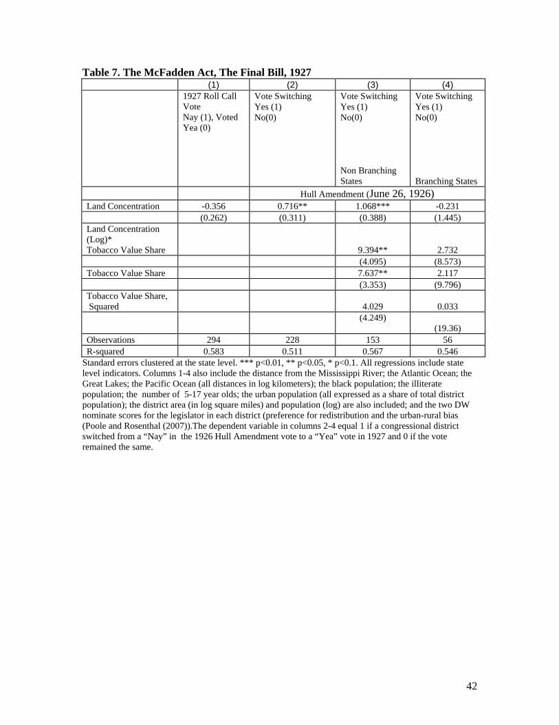
42

Table 7. The McFadden Act, The Final Bill, 1927 (1) (2) (3) (4)

1927 Roll Call Vote Nay (1), Voted Yea (0)

Vote Switching Yes (1) No(0)

Vote Switching Yes (1) No(0) Non Branching States

Vote Switching Yes (1) No(0) Branching States

Hull Amendment (June 26, 1926) Land Concentration -0.356 0.716** 1.068*** -0.231 (0.262) (0.311) (0.388) (1.445) Land Concentration (Log)* Tobacco Value Share

9.394** 2.732 (4.095) (8.573) Tobacco Value Share 7.637** 2.117 (3.353) (9.796) Tobacco Value Share, Squared

4.029 0.033

(4.249)

(19.36) Observations 294 228 153 56 R-squared 0.583 0.511 0.567 0.546

Standard errors clustered at the state level. *** p<0.01, ** p<0.05, * p<0.1. All regressions include state level indicators. Columns 1-4 also include the distance from the Mississippi River; the Atlantic Ocean; the Great Lakes; the Pacific Ocean (all distances in log kilometers); the black population; the illiterate population; the number of 5-17 year olds; the urban population (all expressed as a share of total district population); the district area (in log square miles) and population (log) are also included; and the two DW nominate scores for the legislator in each district (preference for redistribution and the urban-rural bias (Poole and Rosenthal (2007)).The dependent variable in columns 2-4 equal 1 if a congressional district switched from a “Nay” in the 1926 Hull Amendment vote to a “Yea” vote in 1927 and 0 if the vote remained the same.

43

Table 8. The Impact of the McFadden Act in a County Level Cross Section. (1) (2) (3) (4)

VARIABLES

Change in Number of National Banks

Change in Number of National Banks

Change in Share

of National Banks

State Bank Failure Rate, 1927-1930

Branching 3.125* 4.408** 4.042** -0.226 (1.768) (1.712) (1.779) (0.819) Observations 2163 2082 2108 2761 R-squared 0.011 0.031 0.020 0.044

The dependent variable in columns (1) and (2) is the difference between the log of the average number of national banks in county i from 1927-1930 and the log number of national banks in 1926 in county i. Branching is an indicator variable that equals 1 if a state allowed branching, and 0 otherwise, observed in 1920. Column 1 also includes the log number of banks in 1926 in county i as a control variable. Column 2 also includes additional controls include the distance from the Mississippi River; the Atlantic Ocean; the Great Lakes; the Pacific Ocean (all distances in log kilometers); the black population; the illiterate population; the number of 5-17 year olds; the urban population (all expressed as a share of total district population); the district area (in log square miles) and population (log) are also included; and the two DW nominate scores for the legislator in each district (preference for redistribution and the urban-rural bias (Poole and Rosenthal (2007)).The dependent variable in column 3 is the difference in the average share of national banks in county i computed over the period 1927-1930 relative to the share in 1926. Controls include the share of national banks in 1926, as well as the previous geographic and demographic controls in column 2. In column 4, the dependent variable is the average of the annual state bank suspension rate over the period 1927-1930. The annual state bank suspension rate itself is computed as the ratio of the number suspended state banks in the calendar year relative to the total number of state banks the previous year. The controls in column 4 include the state bank suspension rate in 1926, as well as the previous demographic and geographic controls. Standard errors are clustered at the state level. ***, **, * denote significance at the 1, 5 and 10 percent respectively.

44

References Acemoglu, Daron, Simon Johnson, and James A. Robinson, 2005, Institutions as fundamental determinants of long-run growth, in Philippe Aghion and Steven N. Durlauf, eds.: Handbook of Economic Growth Volume 1A (North-Holland Publishing, Amsterdam). Acharya, Viral, Stijn van Nieuwerburgh, Matthew Richardson and Larry White, Guaranteed to Fail: Fannie Mae, Freddie Mac and the Debacle of Mortgage Finance, c) Princeton University Press, March 2011

Adler, Edward. Why Congressional Reforms Fail: Reelection and the House Committee System. Chicago: University of Chicago Press, 2002. Alston, Lee and Joseph Ferrie. Paternalism in agricultural labor contracts in the US South: Implications for the growth of the welfare state. American Economic Review (1993) vol. 83 (4) pp. 852-876 Alston, Lee and Kauffman, Kyle. Agricultural Chutes and Ladders: New Estimates of Sharecroppers and “True Tenants” in the South, 1900–1920. The Journal of Economic History (2009) vol. 57 (02) pp. 464-475 American Bankers Association. (1935). The Bank Chartering History and Policies of the United States. Monograph. Economic Policy Commission. Brown, Craig, and Serdar Dinc, “The Politics of Bank Failures: Evidence from Emerging Markets”, Quarterly Journal of Economics, 2005 (November), 120 (4), 1413-1444. Calomiris, Charles, and Carlos Ramirez, 2004, The political economy of bank entry restrictions: theory and evidence from the US in the 1920s, Columbia University Working Paper. Cartinhour, Gaines Thomson, and Ray Bert Westerfield, 1980, Branch, Group, and Chain Banking. Arno Press: New York, Cetorelli, Nicola and Philip Strahan, “Finance As A Barrier To Entry: Bank Competition And Industry Structure In U.S. Local Markets”, 2006, Journal of Finance 61(1), 437-61. Chapman, John, 1934, Concentration of Banking: The Changing Structure and Control of Banking in the United States (Columbia University Press, New York, NY). Collins, Charles Wallace. 1926. “The Branch Banking Question,” MacMillian, New York. Do, Quy-Toan, 2004, “Institutional Trap”, World Bank working paper.

45

Dehejia, Rajiv and Adriana Lleras-Muney. 2007. “Financial Development and Pathways of Growth: State Branching and Deposit Insurance Laws in the United States from 1900 to 1940”, Journal of Law and Economics, Vol. 50, May. Dinc, Serdar, “Politicians and Banks: Political Influences on Government-Owned Banks in Emerging Markets”, 2005 (August), Journal of Financial Economics, 77, 453-479. Economides, Nicholas, with R. Glenn Hubbard and Darius Palia. The Political Economy of Branching Restrictions and Deposit Insurance: A Model of Monopolistic Competition of Small and Large Banks, Journal of Law and Economics vol. XXXIX (October 1996), pp. 667-704. Engerman, Stanley, and Kenneth Sokoloff, 2002, Factor endowments, inequality, and paths of development among new world economies, Economía 3, 1, 41-109. Engerman, Stanley and Kenneth Sokoloff, 2003, Institutional and non-institutional explanations of economic differences, NBER Working Paper 9989. Fishback, Price. (1989), “Debt Peonage in Postbellum Georgia.” Explorations in Economic History 26, 219–236. Galor, Oded, Omer Moav and Dietrich Vollrath. 2009. “Inequality in Land ownership, the Emergence of Human Capital Promoting Institutions and the Great Divergence” (Review of Economic Studies, 76, 143-179 Glaeser, Edward, Jose Scheinkman, and Andrei Shleifer, 2003, The Injustice of Inequality, Journal of Monetary Economics, Elsevier, vol. 50(1), pages 199-222, January. Goodwyn, Lawrence, 1978, The Populist Moment: A Short History of the Agrarian Revolt in America (Oxford University Press, New York, NY). Haber, Stephen, 2005, Political institutions and financial development: evidence from the economic histories of Mexico and the United States, unpublished manuscript. Haney, L., 1914, Farm credit conditions in a cotton state, The American Economic Review, 14, 1, 47-67. Hicks, John D., 1931, Populist Revolt: A History of the Farmers’ Alliance and the People’s Party (University of Minnesota Press, Minneapolis, MN). Igan, Deniz, Prachi Mishra, and Thierry Tressel, “A Fistful of Dollars: Lobbying and the Financial Crisis”, IMF Working Paper, 2011.

46

Klebaner, Benjamin J. (1990) American Commercial Banking: A History Boston: Twayne Publishers. Kroszner, Randall S. and Philip E. Strahan "What Drives Deregulation? Economics and Politics of the Relaxation of Bank Branching Restrictions."; Quarterly Journal of Economics, 1999, 114(4), pp. 1437-67. Mian, Atif, Amir Sufi and Francesco Trebbi; "The Political Economy of the US Mortgage Default Crisis." American Economic Review, 2010, 100(5), pp. 1967-98. Mitchener, Kris James. “Are Supervision and Regulation Pillars of Financial Stability? Evidence from the Great Depression,” Journal of Law and Economics 50 (May 2007), 273-302, Pred, A., 1966, The Spatial Implication of U.S. Industrial Growth (MIT Press, Cambridge, MA). Preston, H. “The McFadden Banking Act,” American Economic Review (1927) vol. 17 (2) pp. 201-218. Poole, Keith T. and Howard Rosenthal. 2007. Ideology and Congress. Piscataway, N.J.: Transaction Press. Rajan, Raghuram and Rodney Ramcharan, 2010, Land and Credit: A Study of the Political Economy of Banking in the United States in the Early 20th Century, forthcoming, Journal of Finance. Ransom, Roger, and Richard Sutch, 2001, One Kind of Freedom: The Economic Consequences of Emancipation (Cambridge University Press, Cambridge, U.K.). Rusk, Jerrold G. 2001. A Statistical History of the American Electorate. CQ Press: Washington DC. Report of the Comptroller of Currency. 1922. U.S. Federal Reserve Board. Southworth, Donald Shirley. 1928. Branch Banking in the United States. McGraw-Hill: New York.

White, Eugene, “Voting for Costly Regulation: Evidence from Banking Referenda in Illinois, 1924”, Southern Economic Journal, Vol. 51, No. 4 (Apr., 1985), pp. 1084-1098